Does it Cost to be Virtuous? The Macroeconomic Effects of Fiscal Constraints

Does it Cost to be Virtuous? The Macroeconomic Effects of Fiscal

Constraints

Fabio Canova ∗and Evi Pappa†

First version, March 2004This revision, December 2004

Abstract

We study whether and how fiscal restrictions alter the business cycle features of macrovari-ables for a sample of 48 US states. We also examine the ”typical” transmission properties offiscal disturbances and the implied fiscal rules of states with different fiscal restrictions. Fiscalconstraints are characterized with a number of indicators. There are similarities in second mo-ments of macrovariables and in the transmission properties of fiscal shocks across states withdifferent fiscal constraints. The cyclical response of expenditure differs in size and sometimes insign, but heterogeneity within groups makes point estimates statistically insignificant. Creativebudget accounting is responsible for the pattern. Implications for the design of fiscal rules andthe reform of the Stability and Growth Pact are discussed.

JEL classification numbers: E3, E5, H7

Key words: Budget restrictions, Fiscal policy transmission, Policy Rules, Dynamic Panels

∗IGIER, Universitat Pompeu Fabra, and CEPR, Department of Economics, Ramon Trias Fargas 25-27, 08005Barcelona, Spain, email: [email protected]

†London School of Economics and IGIER, Department of Economics, Houghton Street, WC2 2AE London, email:[email protected]. We would like to thank G. Tabellini, R. Perotti, K. West, R. Clarida, J. Frankel, G. Zoega andthe participants of seminars at IGIER and ISOM, Reykjavick for comments and suggestions.

1

1 INTRODUCTION 2

1 Introduction

The size of government deficits and the time path of debt are of central importance in the political

discussions that shape economic policies in OECD countries. For example, in the US active fiscal

policymaking has been limited by frequent disputes between the President and the Congress over

the constitutional balance budget amendment. In Europe, the reform of the Stability and Growth

Pact (SGP) has been a topic of intense debates in the last few years. In the past, membership

to the EMU strongly depended on deficit policies, but initially virtuous countries such as France,

Germany, and the Netherlands have joined ranks with initially less virtuous ones like Italy, Portugal

and Greece in passing the upper bound set for the deficit to GDP ratio. Furthermore, in some

of these countries, the net-of-interest debt to GDP ratio started growing again after the decline

of the late 1990’s. The implications of fiscal policy decisions for the maintenance of monetary

stability have attracted the attention of central bankers and academics have started investigating

how exuberant fiscal policy may affect local and union wide prices (see e.g. Canova and Pappa

(2003)).

Restrictions on fiscal policy actions have been criticized on a number of grounds. Critics often

stress that fiscal constraints limit the ability of governments to react to fluctuations in the local

economy. Two undesirable consequences may result. First, since government capability to stabilize

the economy is reduced, the volatility of macrovariables could be increased. Second, since expendi-

tures must follow the revenue cycle, budget restrictions may make expenditure procyclical. Hence,

tight budget constraints may amplify fluctuations, turning slowdowns into deep recessions.

Despite the popular appeal of this argument, Canzoneri, Diba and Cumby (2002) suggest that

fiscal policy in the US and Europe has hardly focused on macroeconomic stabilization over the last

two decades. Two complementary reasons may account for this. First, given the lags in the leg-

islative process, discretionary fiscal policy may be unable to counteract business cycle fluctuations.

Second, since automatic stabilizers are roughly given at business cycle frequencies, and since their

share in total expenditure is typically large, also the non-discretionary component of expenditure

cannot vary substantially over the cycles. Hence, limiting fiscal actions cannot dramatically alter

the magnitude and the shape of cyclical fluctuations.

Supporters of fiscal restrictions, on the other hand, suggest that the medium term benefits of

limiting government actions dominate the short run costs incurred by the inability of fiscal policy

to react to business cycle conditions (see e.g. Diaz Gimenez, et al. (2003), Andres and Domenec

1 INTRODUCTION 3

(2002)). This argument is usually based on two principles. First, by limiting the ability of govern-

ments to run politically motivated deficits and unsustainable levels of debt, fiscal constraints make

governments more credible, reduce the suboptimality of political games, and induce a smoother

path for taxes, which is the optimal policy to follow in a number of theoretical models (see e.g.

Alesina and Perotti (1996)). Second, since fluctuations in expenditure may have been themselves

a source of undesirable fluctuations, restraining fiscal policy may actually stabilize the economy.

As for the first principle, the literature has made an important distinction between flexible rules,

which allow for some sensitivity of deficit and debt to economic conditions, or apply to consumption

but not to investment and infrastructure expenditures, and strict ones. On the other hand, the

evidence on the contribution of fiscal shocks to macroeconomic fluctuations is contradictory. Stan-

dard dynamic general equilibrium models of fiscal policy (see e.g. King and Baxter (1993), Duarte

and Wolman (2002), or Gali, Lopez Salido and Valles (2003)) have hard time to produce sizable

fluctuations in response to fiscal disturbances in closed economy models calibrated to match salient

features of OECD business cycles. Empirically, Mountford and Uhlig (2002), Canova and Pappa

(2003), and Perotti (2004) have shown that expenditure shocks can at times produce economically

significant output and employment multipliers.

Critics and supporters of fiscal constraints however do agree on one fact: deficits and debts have

distributional effects which may have long lasting repercussions. Borrowing, for example, reduces

resources available to future generations and, if it is used to finance consumption, it may induce

a misallocation of resources. Therefore, the design of fiscal restrictions must carefully balance

incentives and constraints and include intratemporal and intertemporal considerations.

While there is evidence that fiscal restraints have provided some safeguard against the misuse

of public funds (see e.g. Poterba (1994) and Bohn and Inman (1996); Von Hagen (1990) has an

opposite view), very little is known about the macroeconomic consequences of imposing fiscal con-

straints. Gali (1994), Gali and Perotti (2003), Fatas and Mihov (2003), Lane (2003) and Sorensen,

Wu and Yosha (2001) have examined some aspects of the relationship between fiscal variables and

the macroeconomy, but to the best of our knowledge, no empirical study has simultaneously studied

whether fiscal constraints alter (i) the business cycle features of macroeconomic variables, (ii) the

transmission properties of fiscal shocks and (iii) the fiscal rules that governments follow. We can

think of several reasons for why the literature is silent on these questions. First, it is difficult to

find case studies where tight fiscal constraints have been imposed in countries which originally had

no fiscal restrictions. Second, over the cross section, countries which have loose deficit restrictions

1 INTRODUCTION 4

typically have tighter debt constraints. Third, fiscal disturbances are difficult to identify since the

systematic and the unsystematic component of policy are highly intertwined and ”surprises” may

induce macroeconomic changes before they are implemented. Fourth, fiscal rules may be subject

to predictable changes at election times, or at times of political turmoil. Last, but not least, cross

country data is typically short and hard to obtain at the quarterly frequency.

This paper studies how fiscal constraints affect the macroeconomy using data from 48 US states

for the sample 1969-1995. First, we examine whether fiscal constraints alter the volatility and

the comovements of state macroeconomic variables, grouping states with a number of indicators

capturing different aspects of existing fiscal restrictions. Second, we examine the transmission

properties of two types of government expenditure disturbances (one financed by debt and one

by distortionary taxation) for a typical state with loose, or strict fiscal restrictions. Finally, we

back out the typical expenditure rules (one for each type of shock) for states with different fiscal

restrictions and compare them. We use both asymptotic and small sample tests to measure the

statistical significance of the difference in the statistics across groups and corroborate the analysis

by evaluating the economic consequences of the differences we found.

Why use US states to assess the macroeconomic consequences of fiscal constraints? There

are many reasons for our choice. First, the cross section of US states is rich enough to include

cases where rules are strict, others where they are somewhat loose and one case where no fiscal

restrictions are in place (e.g. Vermont). Second, there is one state (Tennessee) where the nature of

fiscal restrictions changed from loose to tight within the sample. Third, the available data covers a

sufficiently long span of time (27 years), including both expansionary and recessionary periods, and

a comparable data set for OECD countries is not available. Finally, deficit and debt constraints

in US states typically exclude capital expenditure. Therefore, they fall within the class of flexible

rules which academics and policymakers consider desirable.

We find that the macroeconomic consequences of fiscal constraints have been overemphasized.

While point estimates and, at times, the sign of the statistics we compute for states with strict

fiscal constraints differ from those of states with loose fiscal constraints, differences are statistically

insignificant and, often, economically unimportant. This result holds regardless of how we define

”loose”, or ”strict”, of whether deficit, debt, or institutional constraints are examined, of the type

of statistical tests we employ and, to a large extent, the statistics and the sample we consider.

For example, standard second moments that the literature has used to characterize business cycle

fluctuations are similar in states with loose and strict restrictions. Furthermore, fiscal restrictions

1 INTRODUCTION 5

have little impact both qualitatively and quantitatively on how fiscal disturbances are transmitted to

the real economy. Finally, fiscal restrictions may not necessarily alter the ability of the government

to respond to the state of the economy and only marginally explain the differences in fiscal rules

across US states.

Why is it that fiscal constraints appear to make so little macroeconomic difference? We show

that the main reason is the ability of state governments to work around the rules and transfer ex-

penditure items to either less restricted accounts, or to less constrained portions of the government.

In addition, the presence of rainy days funds, which are available to all state governments by the

end of the sample, effectively allows to limit current expenditure cuts at times when the constraints

become binding. Given that constraints apply only to a portion of the total budget, that no formal

provision for the enforcement of the constraints exists and that rainy days funds play a buffer-stock

role, it is not surprising to find that tight fiscal constraints do not statistically alter the magnitude

and the nature of macroeconomic fluctuations.

Our results have important implications for the design of fiscal restrictions. If constraints are

imposed to keep government behavior under control, tight restrictions may be the wrong way to go,

since they simply imply more creative accounting practices, unless they come together with clearly

stated and easily verifiable enforcement requirements. That is to say, tight fiscal constraints are

neither a necessary nor a sufficient condition for good government performance. On the other hand,

if constraints are imposed to reduce default probabilities, or to limit the effects that local spending

has on average area wide inflation, and given that their negative macroeconomic effects appear to

be marginal, tight constraints with some carefully selected escape route could be preferable.

Is there a lesson to be learned from the results for the reform of the SGP? While Canova

and Pappa (2003) have shown that the response of macroeconomic variables to fiscal shocks in

the two monetary unions share a number of important similarities, care should be exercised to

use our evidence for that purpose. There are at least three reasons which make most of our

conclusions dubious in a European environment. First, US state labor markets are sufficiently

flexible, people move across states and other margins (such as relative prices) quickly adjust to

absorb macroeconomic shocks. Europe is different in this respect and the imposition of tighter fiscal

restrictions in the EMU may have completely different effects. Second, since fiscal constraints in the

US almost always exclude capital account expenditures, the conclusions we reach are not necessarily

applicable to situations where non-golden rule type of constraints are in place. Third, social security,

medical and welfare expenditures constitute the largest portion of current account expenditure of

2 THE MODEL AND THE METHODOLOGY 6

European countries, while they are a tiny portion of expenditure of US states (less than four

percent). Given that such expenditures are inflexible and, to a large extent, acyclical, direct

extension of our conclusions to the European arena should be avoided. Nevertheless, we would like

to stress that, while the presence of strict fiscal constraints does not make an important difference

for cyclical fluctuations, some fiscal restriction is present in all but one US states. Therefore, none

of our conclusions implies the abandonment of some kind of legislated fiscal restraint.

The rest of the paper is organized as follows. The next section describes the empirical model,

explains our methodology and compares it with those typically used in the literature. Section 3

presents the procedure used to identify fiscal shocks and to construct fiscal rules. Section 4 describes

how indicators capturing deficit and debt restrictions are constructed. Section 5 presents the results

and section 6 compares our results to the existing literature. Section 7 concludes.

2 The model and the methodology

The results presented in this paper are primarily obtained using VARs. While unconditional volatil-

ities and correlations can be obtained without a VAR, we use such a model also for these statistics

to unify our empirical analysis.

We have gathered annual data for 48 US states (DC, Alaska and Hawaii are excluded) for

the period 1969 to 19951. The relative shortness of the data prevents us not only to study the

transmission of shocks across states but also the estimation of a model which simultaneously includes

a number of state and union wide variables. Given these limitations, we are forced to neglect

possible neighborhood effects and choose, for each unit, five endogenous variables, four exogenous

variables and a constant. The endogenous variables are: the log of the state to the union wide

price level; the log of the state to the union wide real per-capita output; the log of the state to

the union wide employment level; the log of state real government revenues and the log of state

real government consumption expenditure, both in per-capita terms and deflated by state prices.

Scaling state variables by their union wide level catches two birds with one stone: it transforms

trending variables into stationary ones; and it allows to directly control for fluctuations which are

aggregate in nature. Note that our scaling does not exclude the possibility that aggregate US

cycles have a spatial dimension, nor the possibility that time series have infrequent mean shifts

1The data stop in 1995, since there is no data on state CPI prices thereafter. We have used an alternativespecification where state CPI prices were substituted with state implicit price deflator data, which are available from1985-2003. We have selected the 1969-95 sample because it is longer and potentially more interesting.


so long as they are shared by the aggregate variables. Note also that we use total state and local

expenditure in the analysis to take into account possible off-budget activities where expenditures

are shifted to less restricted part of the government whenever constraints become binding. The

exogenous variables we employ are the area-wide nominal interest rate, the level of oil prices, the

Federal aid to the states and the state debt to output ratio. The first three variables are used

to control for aggregate area-wide supply and demand effects; local debt enters the specification

following the suggestions of the fiscal theory of the price level (see Christiano and Fitzgerald (2001)

for a survey), and the work of Canova and Pappa (2003). State debt includes both guaranteed and

non-guaranteed debt, to capture possible substitution effects induced by debt limits. The sources

of the data and the definition of the variables are in the appendix. The Schwarz criteria indicates

that one lag of the endogenous variable suffices to capture the dynamics and exogenous variables

enter only contemporaneously in the system, except for debt, which enters with one lag 2.

The literature has typically employed a two-stage strategy to analyze the effects that unit

specific characteristics have on the dynamics of government finances, on the probability of (large)

deficits and, in general, on the relationship between government expenditure and macroeconomic

activity. In the first stage the time series dimension is employed to extract the information on

relevant parameters and, in the second stage, the cross sectional dimension is used to explain

the heterogeneity in estimated parameters using unit specific political, institutional, or economic

characteristics. For example, Bohn and Inman (1996) run a static first stage time series regression

of the type yit = i + αxit + eit for each state, where eit ∼ (0, σ2i ), yit is the state surplus and

xit a vector of macrovariables including output, employment, etc., and then run a cross sectional

regression ˆi = ziγ + vi where zi are observable state characteristics. Sorensen, Wu and Yosha

(2001), Lane (2003) and Fatas and Mihov (2003), on the other hand, run a first stage regression

of the type yit = i + αi∆xit + eit where yit is the budget surplus, the expenditure to output

ratio, the revenue to output ratio, or transformations of them, ∆xit includes contemporaneous, or

contemporaneous and lagged macroeconomic variables and then attempt to explain differences in

αi (or in σi) with cross sectional regressions of the type αi = z1iγ + vi, or σi = σ0 + z2iδ + vi,

where z1i could be different than z2i. While popular, these two-stage procedures produce incorrect

estimates of γ, or δ. In addition, it is hard to predict the direction of bias without knowing exactly

2We have examined variants of the model using e.g, revenues and expenditures measured in percentage of GrossState Product (GSP); GSP per-capita and employment not scaled by union wide averages and state variables ingrowth rates (but not per-capita terms). We have also run a model where instead of fiscal variables we use theresidual of a preliminary regression of these variables on either union wide variables or the variables of the regionwhere the state is located. The results we present are qualitatively invariant to all of these changes.


what is the data generating process of the cross sectional dimension of the panel.

Intuitively, there are three problems. First, specifications like those of Bohn and Inman (1996)

neglect slope heterogeneity: αi may be different from αj if unit i and j regressors are correlated

with individual characteristics (which is likely to be the case if, e.g., xit includes output and zi labor

market, or other national regulations). Neglecting slope heterogeneities produces biased and incon-

sistent estimates of α and, given the structure of the resulting error term, an instrumental variable

(IV) approach is unlikely to solve the inconsistency problem (see e.g. Pesaran and Smith (1995)).

Second, specifications which allow for slope heterogeneities but exclude lagged dependent variables,

like Sorensen, Wu, Yosha (2001), or Lane (2003), omit regressors which are, by construction, corre-

lated with the included ones whenever ∆xit is serially correlated. Lagged dependent variables are

likely to be important in the first stage regression because all fiscal variables are serial correlated.

Omission of lags of the left hand side variable produces biased and inconsistent estimates of the

first stage parameters and therefore renders second stage regression uninterpretable. Also in this

case, an IV approach is unlikely to work since it is difficult to find instruments which effectively

break the correlation between the regressors and the errors. Third, even when slope heterogeneity is

accounted for and lagged dependent variables are included in the first stage regression (as in Fatas

and Mihov (2003)), second stage estimates neglect the fact that bαi (or bσi) have been estimated.Hence, estimates of γ (δ) may be significant even when the ”true” effect is negligible.

To illustrate these problems consider the model

yit = x0it i + x1itαi + eit (1)

αi = x2iγ + vi (2)

where i = 1, 2, . . . , N , x1it is a 1 × K2 vector of exogenous and lagged dependent variables, x2i

is a K2 ×K3 vector of time invariant unit specific characteristics, x0it is a 1 ×K1 vector of unit

specific variables (possibly depending on t) and γ is a K3 × 1 vector of parameters. We assumethat E(x1iteit) = E(x2ivi) = 0 that eit ∼ N(0, σ2i ); that E(eit, ei0τ ) = 0 ∀ t 6= τ and i 6= i0; and

vi ∼ N(0,Σv). Stacking the observations for each i and using (2) into (1) we get yi = x0i i+Xiγ+ i

where Xi = x1ix2i is a T × k3 matrix, and i = x1ivi + ei so that var( i) = x1iΣvx01i + σ2i I ≡ Σ i .

Given Σ i and γ the maximum likelihood estimator of i is i,ML = (x0oiΣ

−1v x0i)

−1(x0oiΣ−1v (yi−Xiγ) and conditional on Σ i , the maximum likelihood estimator of γ is γML = (

PiXiΩ

−1i Xi)

−1

(P

iXiΩ−1i yi) where Ω

−1i = Σ−1

i− Σ−1

ix0i(x0iΣ

−1ix0i)

−1x00iΣ−1i. After some algebraic manipula-

tions one obtains γML = (P

i x02iP−1i x2i)

−1(P

i x02iP−1i αi) where Pi = (x01ix1i)−1Ωi. Hence, γ is a

3 IDENTIFYING FISCAL SHOCKS 9

weighted average of the first stage estimates αi with weights given by Pi.When a two-step approach is used second stage estimates of γ are γ2step = (

Pi x02iΣ

−1v x2i)

−1

(P

i x02iΣ

−1v αi). Therefore, γ2step incorrectly measures the effect of x2i on αi for two reasons. First,

suppose that xi0t = 0, ∀t. Then the term σ−2(x01ix1i) is missing from the formulas of γ2step and

of its standard error (P

i x02iΣ

−1v x2i)

0.5. This means that, while the weights used in γ2step depend

on Σv, those in γML depend on Σi and on the volatility of the unit specific regressors σ−2(x01ix1i).

Second, if xi0t 6= 0, there are additional terms in Ωi, measuring the influence that these regressorshave on αi, which are left out from γ2step. Since the standard error of γ2step is underestimated,

a two-step regression gives an overoptimistic representation of the significance of the relationship.

Moreover, if αi is systematically larger when x1i is more volatile, a positive γ2step may be obtained

even when the true effect is negative. These observations should be kept in mind when comparing

our results with those existing in the literature. In fact, our methodology takes care of all of these

problems. First, lagged dependent variables appear in the model for each state. Second, we allow

for heterogeneity in regression coefficients and in the variances across units. Third, we construct

maximum likelihood estimates of γ by plugging Σv =1

N−1PN

i=1(αi− 1N

PNi=1 αi)(αi− 1

N

PNi=1 αi)

0

and σ2i =1

T−dim(αi)(y0iyi − yixiαi)

2 into the relevant formulas. Our estimators are consistent when

the number of units in each group is large (see e.g. Pesaran and Smith (1995)) and reproduce the

random coefficient Bayesian estimators, when uninformative priors are used.

Since in our case x2i are dichotomous variables, implementing γML is equivalent to calculating

the ”typical” effect separately in states with loose and strict restrictions. Then the equality of

the statistics across groups can be examined using asymptotic χ2-tests, or non-parametric devices

(such as a small sample rank sum test).

3 Identifying Fiscal shocks

To examine the transmission of expenditure shocks and the systematic response of expenditure

to macroeconomic fluctuations we need to identify fiscal shocks. Such an enterprise is typically

complicated and this may explain why only a small number of studies have engaged in such an

activity (see e.g. Ramey and Shapiro (1998), Edelberg, Eichenbaum and Fisher(1999), Mountford

and Uhlig (2002), Blanchard and Perotti (2002), Burnside, Eichenbaum and Fisher (2002), Canova

and Pappa (2003), Pappa (2004), Perotti (2004)).

Three features make fiscal shocks difficult to extract. First, fiscal policy is rarely unpredictable.

A fiscal change is usually subject to long discussions and political debates before it is implemented.


These delays make standard innovation accounting problematic: agents adjust their behavior to

the new conditions when the old regime still prevails; macrovariables start moving before the shock

occurs and no surprise is measurable at the time when the policy change actually takes place. This

”non-fundamentalness” problem plagues fiscal shocks more than other types of policy disturbances.

Second, even when the policy stance is unchanged, expenditures and revenues move in response to

the state of the economy. Therefore, it is necessary to carefully distinguish exogenous shifts from

endogenous reactions to business cycle conditions. Third, since fiscal and monetary policy actions

may be related, identifying fiscal shocks in isolation may produce misleading results.

Our set up is designed to avoid, in principle, all these problems. First, because we consider

a monetary union, we take monetary policy as given when examining state fiscal policy. We do

this by imposing the exogeneity of the economy wide interest rate with respect to state variables.

Second, since all variables are endogenous in the VAR and since we control for both the state of the

local and of the aggregate business cycle, there is no need to produce cyclically adjusted estimates

of fiscal variables. Third, since we precisely define the type of fiscal disturbances we are looking

for and the timing of the responses of the endogenous variables is largely unrestricted, the non-

fundamentalness problem is also considerably eased. In particular, we seek for expenditure shocks

that produce positive comovements in states deficit and in state output (G); and for expenditure

shocks that leave state deficit unchanged and generate negative comovements with state output

(BB).

The first type of expenditure shocks is the one usually encountered in macroeconomic textbooks

and dynamic RBC and New-Keynesian sticky-price models (see e.g. Baxter and King (1993),

or Pappa (2004)): an unexpected increase in spending, financed by bond creation increases, by

definition, state deficits and boosts aggregate demand and output. In identifying this type of

shocks we are agnostic about the behavior of revenues -they are allowed to stay unchanged, or

comove with expenditure as long as the correlation is not perfect - and about the timing of output

responses - they could be contemporaneous, lagged, or leading the shock. However, we assume that

over the horizon of the analysis, distorting taxes are not used to redeem government debt.

The second type of shocks are budget-balanced shocks: expansionary expenditure disturbances

are required to produce an instantaneous increase in revenues so as to leave state deficits unchanged,

and to generate a fall in state output. These dynamics are standard in general equilibrium models of

fiscal policy. For example, Baxter and King (1993) and Ohanian (1997) showed that in a RBC type

model an increase in spending, financed through labor taxation, temporarily decreases consumption


and investment and has protracted negative output effects. While the sign of the output effect is

robust across models, the magnitude of the fall depends on the source of financing (e.g. income

taxes vs. sales taxes), on the elasticity of labor and capital supply to distortionary taxes and on

whether a balance budget is imposed on a period-by-period basis, or if some flexibility is allowed.

Also in this case the timing of the output effect is unrestricted. Hence, anticipatory effects, or future

increases in distorting taxation of the type considered by, e.g., Dotsey (1994), are not a-priori ruled

out. We summarize the identifying restrictions in table 1.

It is incorrect to classify the disturbances we extract as RBC, or Keynesian shocks. For example,

in a simple IS-LM model, balance budget shocks have unitary fiscal multipliers, but this occur

because lump sum taxation is used to finance the expenditure. When distorting taxes are used

the multipliers could be negative also in this case. Our preferred distinction instead focuses on the

form of financing: debt, or lump sum taxes for G shocks, distorting taxes for BB shocks. With this

classification RBC, and traditional, or new-Keynesian models all have the same implications as far

as output and deficits are concerned.

Table 1: Identification Restrictions

Corr(G,Y) Corr (T,Y) Corr (G, Def) Corr(T, Def) Corr(G,T)G shocks > 0 > 0 ≥ 0 but < 1.BB shocks < 0 = 0 = 1

Clearly, we do not expect G and BB shocks to be identified in all states. In theory, G shocks

should be present only in those states which allow deficit carryover and BB shocks only in states

with strict balance budget restrictions. However, balance budget legislation applies only to the

general funds and there is no enforcement mechanism insuring that rules are not bent and non-

guaranteed debt can typically be issued without popular uproar. Therefore, it is possible to have

fiscal disturbances that look like G shocks even in states with tight balance budget rules. Conversely,

debt restrictions may produce disturbances that look like BB shocks even in states with somewhat

loose budgetary restrictions. Finally, one can easily conceive situations where both type of shocks

could be identified in one state (e.g. if different financing restrictions apply to different components

of the budget). Rather than a-priori excluding these possibilities, we let the data tell us whether

there are states which do not conform to the theoretical expectations and condition our analysis

on the results of the identification exercise.

Since our identification procedure, which is based on the sign of the conditional comovements of

expenditure, deficit and output, differs from the one typically used in the VAR literature, it is useful

4 CHARACTERIZING RESTRICTIONS ON GOVERNMENT BEHAVIOR 12

to spend a few words highlighting the advantages of our strategy. The existing literature typically

uses case study approaches, extraneous information, or zero restrictions on the contemporaneous

covariance matrix of VAR shocks to disentangle fiscal shocks from reduced form innovations. Case

studies (see e.g. Ramey and Shapiro (1998), or Burnside, Eichenbaum and Fisher (2002)) are a

powerful way to measure the effect of fiscal surprises if the changes are truly exogenous. As argued

in Perotti (2004), exogeneity is dubious in two of the three typically studied episodes (Korean

War, Vietnam war, Reagan buildup). The identification restrictions we use are theory based, while

those employed in the literature are, to a large extent, conventional and hard to justify with low

frequency data like ours. For example, assuming that it takes more than a period for government

spending to respond to unexpected output movements is unappealing in annual data because of

the presence of automatic stabilizers. Since we do not use zero restrictions, typical endogeneity and

underidentification problems are considerably eased.

To recover shocks with the required characteristics we use the methodology of Canova and

De Nicolo (2002). The approach starts from the eigenvalue-eigenvector orthogonalization of the

variance covariance matrix of VAR residuals and proceeds examining the responses of the endoge-

nous variables to each of the orthogonalized shocks. If we are unable to find expenditure shocks

producing the required comovements in the variables, the eigenvalue-eigenvector decomposition is

multiplied by an orthonormal matrix Q(θ), where θ is a parameter, and the comovements in re-sponse to the new set of shocks are examined. This search process continues, varying θ, or changing

the form of Q(θ) for a fixed θ, until shocks with the required characteristics are found 3.

4 Characterizing restrictions on government behavior

All US states, except Vermont, face some kind of deficit restrictions and the majority of them also

face debt restrictions. However, deficit restrictions are at times loosely formulated; in some cases

they are flexible enough to impose only weak constraints on spending behavior, and in others the

debt limit is large enough to be hardly ever binding. Finally, the enforcement of budget and debt

constraints varies across states. Hence, it is important to appropriately distinguish situations where

constraints are strict from those where they are loose.

3Q(θ) is chosen from the class of rotation matrices, where two directions are rotated at one time. The grid ofθ ∈ (0, π) includes 500 values. More details are in Canova and De Nicolo (2002). By rotating more than two directionsat a time, one can explore systematically the space of identification. Given the computational burden of such anapproach and given that there are 48 states for which such a procedure needs to be run, we have only examinedprimitive bivariate rotations.


As far as deficits are concerned, restrictions can be imposed ex-ante, or ex-post. Ex-ante restric-

tions require the governor to present, or the legislature to approve, a balance budget. Submitting,

or passing a balance budget is a weak constraint since it does not exclude the possibility that, at

the end of the year, the state will actually run a deficit if revenues fall below the expected values.

When ex-ante restrictions are used, statutory, or constitutional provisions for balancing the deficit

may be used to prevent perpetual roll over into the infinite future. Therefore, the timing for bal-

ancing the budget can also serve to induce fiscal discipline. With ex-post rules, the budget has to

be balanced in each fiscal cycle (typically one, at times two years). This means that when economic

activity falls short of expectations, state tax rates must be increased, expenditure cut, or federal

aid collected. If, despite the attempts, a deficit remains it is carried over but is required to be

balanced by the end of the next year. Note that since ex-post rules apply only to the general fund,

balance budget practices may still be unrestricted if it is possible to shift items across accounts, or

funds 4. Furthermore, the presence of rainy days funds, which can be accumulated in expansions

and used to cushion unexpected shortfalls in revenues, may considerably ease the severeness of the

constraints imposed by ex-post rules.

To account for these differences, we follow Bohn and Inman (1996), and construct three indica-

tors capturing different aspects of deficit restrictions. In the first (Ex-ante) an entry of one is given

to states where the governor must submit, or the legislature must pass a balance budget and zero

to the others. In the second (Carryover), an entry of one is given to states which may not carry

over a deficit for more than a year and zero to the rest. In the third (Ex-post), a value of one is

given to states which are required to balance the budget within the current fiscal cycle and zero to

the others (see first three columns of table 2). Here we do not distinguish between constitutional

and statutory restrictions since we wish to measure the effects of fiscal constraints on state activity

and not to design institutions which more effectively limit government actions.

In general, the information contained in the three indices overlaps. For example, among the

12 states with ex-ante budget restrictions, 9 are allowed to carry over deficits for more than one

year. For reference, we also report in table 2 the ACIR (1987) index. This index ranks states on

the basis of the effectiveness of their deficit restrictions, and combines the information contained

in our three indicators using grades from 0 to 10 (with ten being the most effective restrictions),

is a popular choice in the literature. However, if we dichotomize it assigning a one to states with

a grade of eight, or above and a zero to states with a grade of six, or below (as in Sorensen, Wu

4Poterba (1995) reports that in one fourth of US states, budget rules restrict less than 50% of total budget.


and Yosha (2001)), it becomes perfectly collinear with the Ex-post index. Similarly, it becomes

perfectly collinear with the Ex-ante index if a grade of four is used as cut-off point.

As far as debt restrictions are concerned, constraints may refer to the total, or only to the short

run component of debt; they can be fixed in nominal terms, formulated in proportion of revenues,

or the size of the states’ general fund. To capture these differences, we construct three additional

indicators. In the first (Debt1), a value of one is entered to states with some form of debt restriction

and zero to the others. In the second (Debt2), a value of one is attributed to states which either

prohibit guaranteed (full faith and credit) debt, or allow a nominal amount below 200,000 dollars.

A zero is given to all other states. In the third (Shortdebt), a one is given to states which prohibit

short term debt and a zero to the others (see columns 5-7 in table 2).

Finally, we construct three indicators capturing political/legal characteristics which may in-

fluence the state fiscal stance. In the first (Veto), a value of one is given to all states where the

governor has line-item veto power on the budget and zero to the others; in the second (Court) a

value of one is given to states where the Supreme Court is elected by voters and a value of zero if

it is appointed by the Governor, or the legislature and in the third (Constitution) a one is given to

states that need a constitutional amendment to be able to borrow and zero to the others.

As suggested by Mitchell (1967), or Bohn and Inman (1996), these characteristics may affect

the fiscal stance for the following reasons. First, since State Courts are responsible for the enforce-

ment of budget rules, it is conceivable that enforcement is less than perfect and monitoring looser

whenever Courts are appointed by those who also legislate the budget. Second, since constitutional

amendments are much harder to enact than referendums, or simple legislative actions, states with

such restrictions may face considerable constraints in their ability to issue general obligation debt.

Finally, since fiscally conservative voters may held Governors responsible for any marginal

expansion of state budgets, governors seeking reelection may be more active in controlling spending

and deficits. One way to exercise this control is to use the veto power. Hence, as suggested by

Holtz-Eakin (1988), or Carter and Schap (1990), states where the governor has a line-item veto

power may be less prone to run a deficit (see columns 8-10 of table 2).


Table 2: Budget Characteristics of US states

STATEEx-ante Carryover Ex-post ACIRDebt1 Debt2 Short Debt Veto Court ConstitutionAL 0 1 1 10 0 0 1 1 1 1AZ 0 1 1 10 1 1 1 1 0 1AR 0 1 1 9 1 0 1 1 1 0CA 1 0 0 6 0 0 0 1 1 0CO 0 1 1 10 0 0 1 1 0 1CT 1 0 0 5 1 1 0 1 0 0DE 0 1 1 10 1 0 0 1 0 0FL 0 1 1 10 0 0 1 1 0 1GA 0 1 1 10 1 0 0 1 1 1ID 0 1 1 10 1 0 0 1 1 0IL 1 0 0 4 1 0 0 1 1 0IN 0 1 1 10 1 1 1 0 0 1IA 0 1 1 10 1 1 0 1 0 0KS 0 1 1 10 1 0 0 1 0 0KY 0 1 1 10 1 1 0 1 1 0LA 1 0 0 4 1 0 0 1 1 0ME 0 1 1 9 0 0 0 0 0 0MD 1 0 0 6 1 0 0 1 0 0MA 1 0 0 3 1 0 0 1 0 0MI 0 0 0 6 1 0 0 1 1 1MN 0 1 1 8 1 1 0 1 1 0MS 0 1 1 9 1 1 0 1 1 0MO 0 1 1 10 1 0 1 1 0 0MT 1 1 1 10 0 0 0 1 1 0NE 0 1 1 10 1 1 1 1 0 0NV 1 0 0 4 1 1 0 0 1 0NH 1 0 0 2 1 0 0 0 0 0NJ 0 1 1 10 1 1 1 1 0 0NM 0 1 1 10 1 1 1 1 1 0NY 1 1 0 3 0 0 0 1 0 0NC 0 1 1 10 0 0 0 0 1 0ND 0 1 1 8 1 0 1 1 1 0OH 0 1 1 10 1 0 1 1 1 1OK 0 1 1 10 0 0 0 1 1 0OR 0 1 1 8 1 0 0 1 1 1PA 1 0 0 6 1 1 0 1 1 1RI 0 1 1 10 1 1 0 0 0 0SC 0 0 1 10 1 0 1 1 0 0SD 0 1 1 10 1 1 1 1 1 1TN 0 0 1 10 1 0 1 1 1 0TX 1 1 1 8 1 0 0 1 1 1UT 0 1 1 10 1 0 0 1 0 1VT 0 1 0 0 0 0 0 0 0 0VA 0 1 1 8 1 1 1 1 0 0WA 0 1 1 8 1 0 0 1 1 1WV 0 1 1 10 1 0 0 1 1 1WI 0 0 0 6 1 1 0 1 1 1WY 0 1 1 8 1 1 1 1 0 0

5 THE RESULTS 16

5 The Results

5.1 Volatilities and Correlations

To begin with we examine whether basic, reduced form business cycle statistics are affected by the

presence of fiscal restrictions. We summarize cyclical information through 9 statistics: the volatility

of state expenditure, the volatilities of state output, prices and employment in deviation from their

US counterpart; their correlation with per-capita real state consumption expenditure; the mean of

the log consumption expenditure to output ratio and the mean of per capita output.

There are several ways of computing volatilities and correlations. For example, in the business

cycle literature, it is common to filter out long and short frequencies fluctuations and compute

statistics for fluctuations which on average are between 2 to 6 years. In cross unit comparisons,

however, one has to worry about the fact that cycle length may differ in different units. In this

latter case, it is more typical to compute statistics using growth rates of the variables. Here we

present second moments obtained from the residuals of a VAR.

We prefer this approach for two reasons. First, given the short sample, the variability and

correlation properties at business cycle frequencies may be poorly estimated with filtered data.

Second, with the scaling we employ, variables are stationary so moments can be computed without

any further transformation. Finally, by presenting results using the residuals of the VAR, we

account for predictable variations related to the presence of automatic stabilizers which may be

unaccounted for when using raw data.

Table 3 reports the p-values of two tests. The first is an asymptotic χ2-test measuring the dif-

ferences, on average, in each of the statistics across groups of states with different fiscal restrictions.

Since we have nine indicators of fiscal restrictions, different rows report the results obtained with

different classifications. The second is a nonparametric rank sum test, measuring the difference in

the distribution of each of the statistics across groups. Since with some classifications, the number

of units in each group is small; since critical values of such a test have been tabulated for groups

with as little as three units (see e.g. Hoel (1993)), and since the test examines the entire distribu-

tion, as opposed to the first moment, it may be more reliable to evaluate the statistical significance

of the differences.

The message of table 3 is very clear: the presence of tighter budget, debt, or institutional

restrictions does not appear to matter for business cycle fluctuations. In fact, when an asymptotic

test is used, differences across groups are insignificant, regardless of the classification employed to

5 THE RESULTS 17

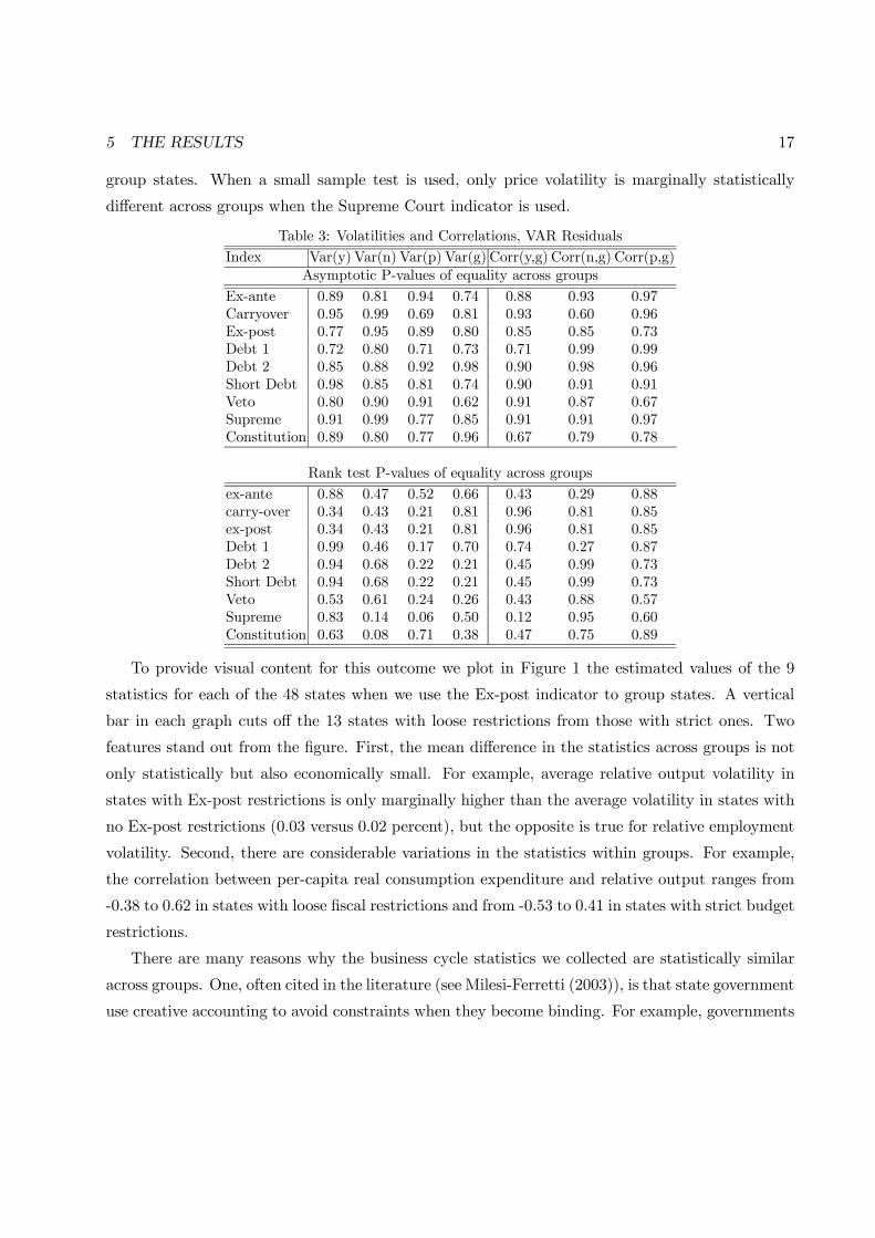
group states. When a small sample test is used, only price volatility is marginally statistically

different across groups when the Supreme Court indicator is used.

Table 3: Volatilities and Correlations, VAR Residuals

Index Var(y) Var(n) Var(p) Var(g) Corr(y,g) Corr(n,g) Corr(p,g)Asymptotic P-values of equality across groups

Ex-ante 0.89 0.81 0.94 0.74 0.88 0.93 0.97Carryover 0.95 0.99 0.69 0.81 0.93 0.60 0.96Ex-post 0.77 0.95 0.89 0.80 0.85 0.85 0.73Debt 1 0.72 0.80 0.71 0.73 0.71 0.99 0.99Debt 2 0.85 0.88 0.92 0.98 0.90 0.98 0.96Short Debt 0.98 0.85 0.81 0.74 0.90 0.91 0.91Veto 0.80 0.90 0.91 0.62 0.91 0.87 0.67Supreme 0.91 0.99 0.77 0.85 0.91 0.91 0.97Constitution 0.89 0.80 0.77 0.96 0.67 0.79 0.78

Rank test P-values of equality across groups

ex-ante 0.88 0.47 0.52 0.66 0.43 0.29 0.88carry-over 0.34 0.43 0.21 0.81 0.96 0.81 0.85ex-post 0.34 0.43 0.21 0.81 0.96 0.81 0.85Debt 1 0.99 0.46 0.17 0.70 0.74 0.27 0.87Debt 2 0.94 0.68 0.22 0.21 0.45 0.99 0.73Short Debt 0.94 0.68 0.22 0.21 0.45 0.99 0.73Veto 0.53 0.61 0.24 0.26 0.43 0.88 0.57Supreme 0.83 0.14 0.06 0.50 0.12 0.95 0.60Constitution 0.63 0.08 0.71 0.38 0.47 0.75 0.89

To provide visual content for this outcome we plot in Figure 1 the estimated values of the 9

statistics for each of the 48 states when we use the Ex-post indicator to group states. A vertical

bar in each graph cuts off the 13 states with loose restrictions from those with strict ones. Two

features stand out from the figure. First, the mean difference in the statistics across groups is not

only statistically but also economically small. For example, average relative output volatility in

states with Ex-post restrictions is only marginally higher than the average volatility in states with

no Ex-post restrictions (0.03 versus 0.02 percent), but the opposite is true for relative employment

volatility. Second, there are considerable variations in the statistics within groups. For example,

the correlation between per-capita real consumption expenditure and relative output ranges from

-0.38 to 0.62 in states with loose fiscal restrictions and from -0.53 to 0.41 in states with strict budget

restrictions.

There are many reasons why the business cycle statistics we collected are statistically similar

across groups. One, often cited in the literature (see Milesi-Ferretti (2003)), is that state government

use creative accounting to avoid constraints when they become binding. For example, governments

5 THE RESULTS 18

may shift expenditure items off-the-budget, or to less restricted branches (e.g. local governments),

or use stabilization funds to limit the revenue crunch they may experience in recessions. Similarly,

debt restrictions apply only to guaranteed debt. Hence, there is an incentive for state governments

to swap non-guaranteed (revenue) for guaranteed debt when the borrowing limit becomes binding.

Since our data includes both local and state expenditures and we consider total outstanding debt, we

can study whether fiscal restrictions constraint government behavior, or simply imply substitution

toward less restricted accounts, bonds, or practices.

Var(y)

0 250.0000

0.0008

0.0016

0.0024

Var(n)

0 250.00000

0.00016

0.00032

0.00048

Var(p)

0 250.000000

0.000035

0.000070

0.000105

Mean(log(g/y))

States0 25

-2.8

-2.4

-2.0

-1.6

Corr(y,g)

0 25-0.70

-0.35

0.00

0.35

0.70

Corr(n,g)

0 25-0.7

0.0

0.7

1.4

Corr(p,g)

0 25-0.6

0.0

0.6

1.2

mean(ypc)

States0 25

0

7000

14000

21000

Figure 1: Moments using the Ex-post classification

Table 4, which reports first and second moments of the level of total state and local deficits

and debt, of debt to output ratios and of the growth rate of non-guaranteed to guaranteed debt,

is consistent with the idea that more restricted governments tend to substitute across accounts to

avoid the restrictions. In fact, the mean deficits appear to be different in strongly restricted vs.

weakly restricted states only when the short term debt indicator is used and the rank test is used to

evaluate the differences while the debt to output ratio is significantly different only when the Debt2

indicator is used. Perhaps surprisingly, we also find that the growth rate of non-guaranteed to

5 THE RESULTS 19

guaranteed debt is not significantly different across groups of states with different debt constraints.

While this appears to be in contrast with the substitution hypothesis, one should also notice that

both types of states have substantially increased the less unrestricted form of debt financing over

time and this may account for our failure to detect differences.

Table 4: Means and Volatilities

Index Mean(df) Mean(Debt)Mean(Debt/Y)Mean(∆ NG/G) vol(df) vol(debt) vol(Debt/Y) vol(∆ NG/G)Asymptotic test: P-values for the null of equality of means across groups

Ex-ante 0.85 0.85 0.99 0.88 0.58 0.69 0.52 0.68Carryover 0.86 0.99 0.85 0.98 0.96 0.98 0.89 0.89Ex-post 0.49 0.87 0.97 0.80 0.96 0.95 0.96 0.91Debt 1 0.88 0.98 0.92 0.91 0.73 0.78 0.95 0.67Debt 2 0.92 0.93 0.63 0.85 0.82 0.84 0.87 0.74Short Debt 0.81 0.85 0.99 0.74 0.56 0.56 0.99 0.91Veto 0.82 0.94 0.97 0.77 0.95 0.97 0.62 0.68Supreme 0.83 0.99 0.91 0.89 0.96 0.93 0.97 0.76Constitution 0.92 0.92 0.86 0.78 0.87 0.90 0.80 0.64

Rank sum test P-values for the null of equality of distributions across groups

Ex-ante 0.58 0.72 0.61 0.17 0.68 0.16 0.98 0.07Carryover 0.96 0.57 0.60 0.57 0.11 0.98 0.87 0.76Ex-post 0.51 0.05 0.88 0.81 0.96 0.27 0.79 0.53Debt 1 0.55 0.03 0.66 0.83 0.40 0.36 0.91 0.97Debt 2 0.29 0.77 0.03 0.96 0.68 0.94 0.43 0.31Short Debt 0.03 0.66 0.82 0.94 0.62 0.29 0.94 0.01Veto 0.24 0.79 0.97 0.46 0.97 0.12 0.66 0.08Supreme 0.09 0.43 0.91 0.16 0.37 0.85 0.67 0.22Constitution 0.59 0.45 0.86 0.82 0.22 0.75 0.80 0.87

A further piece of evidence on this issue comes from figure 2 where we plot the average (across

states) ratio of local to state expenditure over time. Three features deserve comments. First,

there has been a significant trend increase in the expenditure of the less restricted branches of the

government in the 1990’s and this pattern is shared by states with strict and loose fiscal restrictions.

Second, states which are less restricted have local expenditure which is consistently smaller than

states where Ex-post restrictions are in place - on average about 15 percent. Third, both types

of states tend to resort to local expenditure more during periods of national wide recessions (see

1980-81 and 1990-91).

Overall, the evidence is supportive of the claim that tight fiscal restrictions have not produced,

on average, more virtuous governments and, as a consequence, have not altered the business cycle

properties of state variables. The conclusions is robust to the classification used to define states

5 THE RESULTS 20

with tight fiscal restrictions and, to a large extent, of the tests used to evaluate the mean differences

across groups and the statistics employed. We also argue that this outcome seems due to the fact

that state governments have the ability to bend the rules and use creative accounting to avoid the

constraints.

1

1.051.1

1.15

1.2

1.251.3

1.35

1.41.45

1.5

1977 1981 1985 1989 1993 1997

no res tric t ionsres tric t ions

Figure 2: Average Local to State Expenditure

While the evidence seems overwhelming, one important caveat needs to be mentioned: the

conclusions we have drawn are so far based on ”reduced form” statistics. Although volatilities and

correlations are unaffected by budget restrictions it is possible that the channels through which fiscal

policy shocks are transmitted to the state economy could be significantly altered. In addition, tight

budget, debt, or institutional restrictions may imply different fiscal rules. Since our VAR model can

exactly examine these issues, we next turn to a more structural evaluation of the macroeconomic

effects of fiscal constraints.

5.2 The transmission of expenditure shocks

The identification of structural expenditure shocks roughly produced the expected results. We

identify G disturbances in 36 states and BB disturbances in 12 states; in seven states (Connecticut,

Iowa, Louisiana, Oklahoma, Rhode Island, Tennessee, Virginia) we fail to recover any expenditure

shock and in seven states (Kansas, Maryland, Mississippi, South Carolina, Utah, Washington,

West Virginia) we identify both G and BB shocks. We have already mentioned that, since our data

includes state and local consumption expenditure, and since expenditure switching practices seem

5 THE RESULTS 21

to be widespread, shocks in states with strict constraints may end up looking like G shocks. We

find that this is the case in 25 states. We also mentioned the possibility that states with no strict

budget requirement may nevertheless maintain close to a balance budget when manipulating the

discretionary component of expenditure. This seems to be the case in Maryland and Pennsylvania.

How is it that in some states both shocks are identified and in others no shocks satisfy the restrictions

we imposed? We conjecture that structural instability is responsible for both results. In fact, in

states were no expenditure shock is identified, the comovements of expenditure, deficit and output

are poorly estimated. On the other hand, the seven states where both shocks are identified are

among the last to establish stabilization funds 5 and the variability of BB shocks in these states

declines considerably in the last 10 years of the sample.

We measure the transmission of expenditure shocks to the local economy for a ”typical” state

with strict, or loose budget restrictions using the one step methodology described in section 2.

We computed ”typical” responses grouping states with our nine indicators. Since conclusions are

broadly robust, we only present outcomes obtained using the Ex-post indicator and the Debt2

indicator. Figure 3 plots the mean response and a 68% confidence band of relative output (first

row), relative employment (second row) and relative prices (third row) following a G shock and

Figure 4 the same information following a BB shock when the Ex-post index is used. Figures 5

and 6 plot bands for the two types of shocks when the Debt2 indicator is used to classify states.

Consider Figure 3. Qualitatively speaking, the responses of the three variables to G shocks

conform with theoretical expectations: expansionary expenditure shocks boost aggregate demand

and increase, on average, relative employment in both groups of states. The pattern of relative

price responses is slightly different across columns: in fact, relative prices rise instantaneously

when strict restrictions are in place while are instantaneously insignificant in states with loose

restrictions. However, in both cases responses are positive after two years and remain persistently

and significantly above the trend for another 5 years.

A BB type disturbance, on average, significantly decreases relative employment in both group of

states. Also this pattern conforms to theoretical expectations since an expenditure increase, when

financed by distortionary taxation, is expected to have contractionary effects on output. Relative

price movements are insignificant over the first two years for both groups of states but then turn

positive and slightly different from zero in states with strict deficit restrictions.

5In Kansas stabilization funds were introduced in 1993, in Maryland in 1985, in Missisipi in 1982, in Utah in 1986,in West Virgina in 1981 and in Washigton in 1981.

5 THE RESULTS 22

G shocksStrict Deficit Restrictions

Out

put

0 5-0.16

0.00

0.16

0.32

0.48

0.64

Em

ploy

men

t

0 5-0.09

0.00

0.09

0.18

0.27

Pric

es

0 5-0.016

0.000

0.016

0.032

0.048

0.064

Loose Deficit Restrictions

0 5-0.1

0.0

0.1

0.2

0.3

0 5-0.05

0.00

0.05

0.10

0.15

0.20

0 5-0.075

-0.050

-0.025

0.000

0.025

0.050

Figure 3: Responses of Macroeconomic Variables, Ex-Post Classification

The typical responses of output and employment to both shocks in the two groups are also

quantitatively similar. Take, for example, G shocks. Here the maximum difference in the output

and employment responses for the two groups are 0.12 and 0.06, respectively. But the mean response

of the two variables for the typical state with strict restrictions is inside the band obtained for the

typical state with loose restrictions and the bands for the two groups of states largely overlap.

Furthermore, the qualitative difference in relative price responses we have noted, washes out once

standard errors are accounted for.

Two other interesting features of figures 3 and 4 need to be emphasized. First, the timing of

the responses is largely unaltered by the presence of strict budget restrictions: the largest response

of relative output and relative employment is always instantaneous, while the response of relative

prices is slightly hump shaped. Second, the persistence of the responses also looks similar across

groups for both types of shocks. For example, the half-life of the output responses to G shocks is

about two years for both groups while it is one year for both groups with BB shocks.

Is there any possibility that, although statistically insignificant, difference across groups are

5 THE RESULTS 23

economically relevant? Figures 3 and 4 are not very informative on this issue. For example,

comparing point estimates it looks as if cumulative one year output multipliers for both types

of shocks are about 20% larger in states with strict fiscal restrictions. However, any meaningful

attempt to explain this difference (for example, noting that large fiscal shocks are less likely to

occur when strict fiscal constraints are in place) comes against the fact that the uncertainty around

point estimates is sufficiently large to make the two multipliers indistinguishable.

BB shocksStrict Deficit Restrictions

Out

put

0 5-2.0

-1.5

-1.0

-0.5

0.0

0.5

Empl

oym

ent

0 5-0.4

-0.2

0.0

0.2

Pric

es

0 5-0.032

-0.016

0.000

0.016

0.032

0.048

Loose Deficit Restrictions

0 5-0.8

-0.6

-0.4

-0.2

-0.0

0.2

0 5-0.54

-0.36

-0.18

-0.00

0.18

0 5-0.3

-0.2

-0.1

-0.0

0.1

0.2

Figure 4: Responses of Macroeconomic Variables, Ex-Post Classification

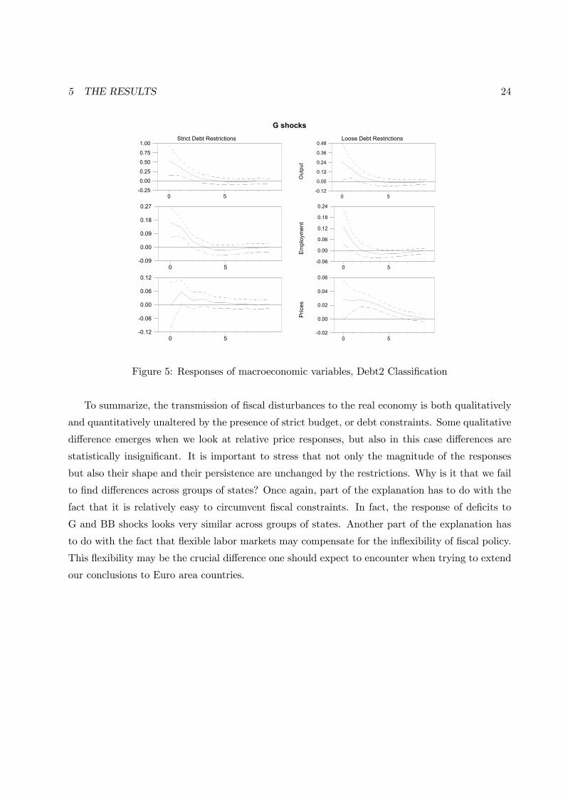
Figures 5 and 6 confirm these conclusions. The only noticeable difference across states with

strict/ loose debt restrictions concerns the behavior of employment with BB shocks. In fact, it

appears that employment is better shielded from the adverse economic effects of balance budget

shocks when loose debt constraints are in place. Also in this case, standard error bands largely

overlap making differences at several horizons statistically insignificant.

5 THE RESULTS 24

G shocksStrict Debt Restrictions

0 5-0.25

0.00

0.25

0.50

0.75

1.00

0 5-0.09

0.00

0.09

0.18

0.27

0 5-0.12

-0.06

0.00

0.06

0.12

Loose Debt Restrictions

Out

put

0 5-0.12

0.00

0.12

0.24

0.36

0.48

Em

ploy

men

t

0 5-0.06

0.00

0.06

0.12

0.18

0.24

Pric

es

0 5-0.02

0.00

0.02

0.04

0.06

Figure 5: Responses of macroeconomic variables, Debt2 Classification

To summarize, the transmission of fiscal disturbances to the real economy is both qualitatively

and quantitatively unaltered by the presence of strict budget, or debt constraints. Some qualitative

difference emerges when we look at relative price responses, but also in this case differences are

statistically insignificant. It is important to stress that not only the magnitude of the responses

but also their shape and their persistence are unchanged by the restrictions. Why is it that we fail

to find differences across groups of states? Once again, part of the explanation has to do with the

fact that it is relatively easy to circumvent fiscal constraints. In fact, the response of deficits to

G and BB shocks looks very similar across groups of states. Another part of the explanation has

to do with the fact that flexible labor markets may compensate for the inflexibility of fiscal policy.

This flexibility may be the crucial difference one should expect to encounter when trying to extend

our conclusions to Euro area countries.

5 THE RESULTS 25

BB shocksStrict Debt Restrictions

Out

put

0 5-1.6

-1.2

-0.8

-0.4

-0.0

0.4E

mpl

oym

ent

0 5-0.64

-0.48

-0.32

-0.16

0.00

0.16

Pric

es

0 5-0.02

0.00

0.02

0.04

Loose Debt Restrictions

0 5-2.7

-1.8

-0.9

-0.0

0.9

0 5-0.3

0.0

0.3

0.6

0 5-1.0

-0.5

0.0

0.5

1.0

Figure 6: Responses of macroeconomic variables, Debt2 Classification

5.3 Fiscal rules

To analyze the systematic component of expenditure we compute the contemporaneous policy rules

implied by our structural VAR estimates for each group of states 6. We report in table 5 average

point estimates of the coefficients on output, employment, prices and debt/output ratio for each of

the indicators used to group states. For interpretation purposes coefficients are normalized so that

expenditure appears on the left hand side with a unitary coefficient.

Several interesting features emerge from the table. First, it appears that different type of shocks

imply different expenditure rules. With G shocks, expenditure is generally leaning against relative

output, relative employment and debt while it is roughly unresponsive to relative prices. When BB

shocks are considered, expenditure follows relative output, leans against relative price movements

and is roughly unresponsive to the other two variables.

Second, while there are some changes in the sign of the output coefficient across classifications,

in many cases, only magnitude differences are present. For example, for G shocks, expenditure

6This is achieved computing the policy rule for each state, given the identification scheme. The policy rule for atypical state of each group is calculated weigthing each state’s coefficients by their standard deviations as describedin section 2.

5 THE RESULTS 26

is always leaning against relative output movements when loose restrictions are in place and it is

following relative output movements when strict restrictions are in place only with the three debt

Table 5: Government expenditure rules

Index Output Prices Employment DebtG Shocks

Ex-ante loose restrictions -0.24 0.93 -2.41 -0.12strict restrictions -0.21 0.00 -0.12 -0.82

Carry-over loose restrictions -0.14 -0.03 -0.03 -0.23strict restrictions -0.31 1.25 -3.20 -0.45

Ex-post loose restrictions -0.16 0.01 -0.08 -0.47strict restrictions -0.38 2.21 -5.53 -0.03

Debt 1 loose restrictions -3.70 10.64 2.94 -2.82strict restrictions 0.16 -0.52 -2.21 -0.06

Debt 2 loose restrictions -1.92 1.83 0.16 -0.59strict restrictions 1.80 -0.81 -3.88 -0.05

Short Debt loose restrictions -0.24 0.57 -1.01 -0.26strict restrictions 1.81 -0.81 -3.76 -0.05

Veto loose restrictions -0.08 0.003 -0.06 -0.06strict restrictions -0.41 1.38 -3.59 -0.68

Court loose restrictions -0.12 -2.75 0.43 0.73strict restrictions -0.20 -0.30 -1.09 -0.05

Constitution loose restrictions -0.32 -1.15 0.43 0.73strict restrictions -0.28 -0.88 0.09 0.18

BB ShocksEx-ante loose restrictions 4.92 -5.42 0.05 0.10

strict restrictions 8.29 -0.15 -6.13 -0.47Carry-over loose restrictions 17.42 0.29 -8.98 -1.11

strict restrictions 5.48 -4.64 -0.40 0.14Ex-post loose restrictions 19.94 -0.41 -15.09 -1.41

strict restrictions 3.88 -4.25 0.03 0.11Debt 1 loose restrictions 0.15 0.01 -0.01 0.16

strict restrictions 7.34 -4.64 -2.38 -0.13Debt 2 loose restrictions 8.09 -3.58 -2.48 -0.01

strict restrictions 2.55 -4.02 -1.03 -0.19Short Debt loose restrictions 8.32 -0.00 -3.52 -0.12

strict restrictions 0.36 -12.74 1.85 0.03Veto loose restrictions 5.97 -3.75 -1.93 -0.08

strict restrictions -0.12 -2.75 0.43 0.73Court loose restrictions 7.34 -8.88 1.71 -0.19

strict restrictions 5.06 -0.34 -4.36 -0.00

Constitution loose restrictions 1.32 -0.69 -0.12 -0.06strict restrictions 2.28 -0.93 -0.61 -0.18

classifications. Expenditure also follows relative output movements for both groups of states when

BB shocks are considered with eight of the nine indicators and it is only with the Veto indicator

5 THE RESULTS 27

that strict restrictions imply countercyclical responses.

Third, the signs of employment and price coefficients depend, to a large extent, on the clas-

sification used and the magnitude of variations is considerable. For example, with G shocks the

average relative price coefficient for states with loose restrictions runs from -2.75 to 10.64 and the

one for states with strict restrictions runs from -0.81 to 2.21.

Fourth, expenditure systematically responds in a stabilizing fashion to debt/output ratio in

both groups of states when G shocks are examined with all but one indicator. The magnitude of

the average estimated elasticity ranges from 0.05 to a large 2.82, and it is not necessarily true that

states with strict fiscal rules react differently, on average, to debt. A more mixed pattern instead

emerges when BB shocks are considered: the signs change across classifications in a somewhat

unpredictable manner and no pattern is detectable.

But perhaps more importantly, regardless of the classification used to group states and of the

type of shocks considered, and even in those cases when sign switches are present, differences

across groups of states are statistically insignificant. This is true both when average coefficients

are significantly different from zero and when they are not and occurs because policy rules within

groups are very heterogeneous. As an illustration, take the Ex-post classification. There average

relative prices and relative employment coefficients are equal to -0.08 and 0.01 respectively, (with

standard errors equal to 1.82 and 1.32) when no restrictions are in place, implying, for example, that

a one percent movement in state employment above the national level makes per-capita expenditure

fall by less than 0.1 percent. Expenditure becomes strongly countercyclical with respect to relative

employment movements and turns procyclical with respect to relative prices movements, on average

when restrictions are in place (coefficients are -5.53 and 2.21, respectively). However, standard

errors are large also in this case (equal to 2.70 and 1.61, respectively) making confidence bands

around the mean largely overlap.

What does the large heterogeneity within group tell us about fiscal rules? It appears that

deficit, debt and political restrictions only marginally account for the differences in expenditure

responses to business cycle conditions across states. To put this result in another way, the R2 in a

typical two-stage regression where fiscal dummies are used to explain differences in the first stage

slope estimates is negligible. This suggest that other state characteristics (e.g. their location, the

composition of output, or the trade pattern with neighboring states) could be more important to

explain differences in the cyclical responses of state expenditure to movements in macro variables.

6 COMPARING OUR RESULTS TO THE LITERATURE 28

6 Comparing our results to the literature

Our results differ from some of those present in the literature. Therefore, it is important to highlight

the reasons which may account for the differences. As mentioned the more structural part of our

analysis is novel and no comparison with the literature is available. For the reduced form analysis,

one should also remember that the extent of the overlap is limited, since the literature has not

focused on volatilities and correlations.

For the latter type of analysis, there is one econometric reason, already mentioned in section 2,

which may account for the differences: we use one-step estimators while the literature has employed

two-steps estimators for models like those in equations (1)-(2). Since our estimators are consistent

in a variety of circumstances and efficiently account for uncertainty in the first stage estimates, the

significance of the difference found in the literature across groups of states could be artificial.

There are two other reasons which may help to understand why our results are different: the

treatment of aggregate cycles and that of dynamic heterogeneities.

All our results are obtained scaling state macroeconomic variables by their US average since

this allows us to explicitly account for fluctuations which are nationwide in nature. Such a scaling

is not typically employed in the literature and the list of economy wide variables used to control for

these factors is either short, or inexistent. Hence, what appeared as different economic relationships

in states with strict, or loose fiscal restrictions could be biases induced by the omission of effective

controls for economy wide business cycles.

We have also mentioned in section 2, the need to control for dynamic heterogeneity in the

analysis. It is often argued that US states are relatively homogeneous and that fixed effects suffice

to account for the differences. To show that this is far from being the case, we computed output

volatility separately pooling data for states with and without Ex-post restrictions. A test for

the significance of the differences in the two groups has now a p-value of 0.04 (as opposed to

0.77 as reported in table 4), suggesting that dynamic heterogeneities within each group of states

are very important. Since failure to take dynamic heterogeneities into account causes biases and

inconsistencies, differences between our results and those presented in the literature can also be

due to the poor properties of the estimators others have used.

7 CONCLUSIONS 29

7 Conclusions

This paper analyzed whether tight fiscal constraints affect the macroeconomic performance of 48

US states for the period 1969-1995. First, we studied the volatility and the comovements of a

number of state variables. In each case we constructed a mean estimator for groups of states with

different fiscal constraints and evaluated the statistical and economic significance of the differences.

Second, we examined the differences in the transmission properties of expenditure disturbances

financed by debt, or by distortionary taxation for a typical state with, or without fiscal restrictions.

Finally, we backed out expenditure rules (one for each of the two shocks) for states with loose and

strict restrictions and compared them.

We find that the macroeconomic consequences of fiscal constraints have been overemphasized.

While the sign and the magnitude of point estimates are, at times, different, these differences are

statistically insignificant and economically unimportant. Our conclusions are robust in a number of

dimensions, and in particular, do not depend on the way we define ”loose”, or ”strict”, on whether

deficit, debt, or institutional constraints are in place, on the type of statistical tests we employ and,

to a large extent, on the statistics we consider.

We argue that the main reason for why fiscal constraints make so little difference for macroe-

conomic fluctuations is the ability of state governments to work around the rules and transfer

expenditure items to either less restricted accounts, or to less constrained portions of the govern-

ment. In addition, the presence of rainy days funds effectively allows to limit current expenditure

cuts at times when the constraints become binding. Given that constraints apply only to a portion

of the total budget, that no formal provision for the enforcement of the constraints exist and that

rainy days funds play a buffer-stock role, it is not surprising to find that tight fiscal constraints do

not statistically alter the magnitude and the nature of macroeconomic fluctuations.

Our results have important implications for the design of fiscal restrictions. If constraints are

imposed to keep government behavior under control, tight restrictions may be the wrong way to go,

since they simply imply more creative accounting practices, unless they come together with clearly

stated and easily verifiable enforcement requirements. That is to say, tight fiscal constraints are

neither a necessary nor a sufficient condition for good government performance. On the other hand,

if constraints are imposed to reduce default probabilities, or to limit the effects that local spending

has on average area wide inflation, and given that their negative macroeconomic effects appear to

be marginal, tight constraints with some carefully selected escape route could be preferable.

7 CONCLUSIONS 30

Although it is tempting to do so, we should warn the reader against using the evidence to draw

conclusions about the reform of the SGP. And we would like to do this despite the fact that Canova

and Pappa (2003) have shown that the response of macroeconomic variables to fiscal shocks in

the two monetary unions share a number of important similarities. Three reasons motivate our

concerns. First, labor markets in the US are sufficiently flexible, people move and other margins

(such as relative prices) adjust to absorb macroeconomic shocks. Europe is different in this respect

and the imposition of tighter fiscal restrictions in the EMU may have completely different effects.

Second, since fiscal constraints in the US almost always exclude capital account expenditures, the

conclusions we reach are not necessarily applicable to situations like EMU where non-golden rule

type of constraints are in place. Third, social security, medical and welfare expenditures constitute

the largest portion of current account expenditure of European countries, while they are a tiny

portion of expenditure of US states. Furthermore, we would like to underscore that none of our

conclusions implies the abandonment of some kind of legislated fiscal restraint and that fiscal

constraints can have beneficial distributional and long run effects.

7 CONCLUSIONS 31

Appendix A: Data sources and definitions

US data are annual from 1969 to 1995, real, seasonally adjusted and per capita. U.S. Census

Bureau is the source unless it is otherwise indicated.

State Population: total state population in thousands.

Gross state product (in constant 1982 prices): Obtained from Bureau of Economic Analysis

(BEA) from 1977; before 1977 we used the series from Oved Yosha’s US State-Level Macroeconomic

Databank (www.tau.ac.il/yosha ).

State revenue: total state and local revenue.

State expenditure: Direct expenditure - capital outlays. Direct expenditure measures all expen-

ditures other than intergovernmental expenditures. It includes both state and local expenditures

and covers all funds available to the state government.

State debt : total state and local debt outstanding at the end of the fiscal year. It includes short

term debt and long run guaranteed and non-guaranteed (revenue bonds) debt. The decomposition

of long run total debt into two components is available only from 1977.

State employment: total full and part time state and local employment (from BLS).

State Prices: State prices are from Del Negro (1998). The price level for state i is computed as:

Pit = wui P

uit+(1−wu

i )PRit where P

Rit denotes the price level in rural areas of state i and comes from

the Monthly Labor Review data of the Bureau of Labor Statistics (after 1978) and the ”cost of

living for intermediate level budget” from the same source (before 1978). wui measures the fraction

of population living in rural areas of state i and comes from the Statistical Abstract of the US.

Puit is constructed as P

uit =

PKk=1 ω

ki P

kit + (1 −

PKk=1 ω

ki )P

Bit where P

kit is the CPI in metropolitan

area k obtained from the ACCRA (American Chamber of Commerce Realtors Association) and the

Bureau of Labor Statistics data on CPI for Urban Consumers (CPI-U) and CPI by Regions and

by Urban Population and ωki is the percentage of urban population living in metropolitan area k

obtained from the Bureau of Economic Analysis site. PBit is the CPI in other urban areas taken

from the Monthly Labor Review data of the Bureau of Labor Statistics. State CPI is normalized

so that in each year their population average coincides with the US CPI.

Federal Aid Total: total aid provided to local and state governments by the Federal Govern-

ment.

State GSP Deflators: Computed from real and nominal state GSP data (from BEA).

US aggregate data for real GDP, interest rates, CPI and oil prices come from the Federal Reserve

Bank of St. Louis FREDII data bank. Data on aggregate population and federal aid to comes from

the US Census.

8 REFERENCES 32

8 References

Alesina, Alberto and Perotti, Roberto (1996) ”Budget Deficit and Budget institutions”, NBER

working paper 5556

Andres, Javier and Domenec, Rafael (2002), ”Automatic Stabilizers and Monetary Rules in a

Ricardian Economy”, Universidad de Valencia, mimeo.

Bohn, Henning and Inman, Robert (1996) ”Balance Budget Rules and Public Deficits: Evidence

from the US”, Carnegie Rochester Conference Series in Public Policy, 45, 13-76.

Baxter Marianne and Robert King(1993), ”Fiscal Policy in General Equilibrium,” American Eco-

nomic Review, 83, 315-335.

Blanchard Olivier and Roberto Perotti (2002): ”An Empirical Characterization of the Dynamic Ef-

fects of Changes in Government Spending and Taxes on Output,” Quarterly Journal of Economics,

117, 1329-1368.

Besley Timothy and Anne Case (1995) ”Does Political Accountability Affect Economic Policy

Choices? Evidence from Gubernatorial Term Limits” Quarterly Journal of Economics, 110, 769-

798.

Canova Fabio and Gianni De Nicolo’ (2002), ”Money matters for Business Cycle Fluctuations in

G-7,” Journal of Monetary Economics, 49, 1131-1159.

Canova, Fabio and Evi Pappa (2003), ” Price Differentials in Monetary Unions: The role of fiscal

shocks ”, CEPR working paper 3746.

Carter, John and Schop, David (1990), ”Line-Item Veto: Where is thy string?” Journal of Economic

perspective, 4, 103-118.

Canzoneri, Matthew., Cumby, Robert and Diba, B (2002), ”Should the European Central Bank

and the Federal reserve be Concerned about Fiscal Policy?”, paper presented at the Federal Reserve

Bank of Kansas City’s Symposium ”Rethinking Stabilization Policy.”

Christiano Lawrence and Terry Fitzgerald (2000) ”Understanding the Fiscal Theory of the Price

Level,”, NBER Working Paper 7668.

Del Negro Marco (1998), ”Aggregate Risk Sharing Across US States and Across European Coun-

tries,” Yale University, mimeo.

Diaz Gimenez, Javier, Giovannetti, Giorgia., Marimon, Ramon and Teles, Pedro (2003) ”Nominal

Debt as a Burden to Monetary Policy”, UPF mimeo.

Edelberg, Wendy, Martin Eichenbaum and Jonas Fisher (1999) ”Understanding the effects of a

Shocks to Government Purchases”, Review of Economic Dynamics, 2, 166-206.

Duarte Margarida and Alexander Wolman (2002), ”Regional Inflation in a Currency Union: Fiscal

Policy vs. Fundamentals,” mimeo Federal Reserve Bank of Richmond.

Dotsey, Mike (1994) ” Some Unpleasant Supply Side Arithmetic”, Journal of Monetary Economics,

33, 507-524.

Fatas Antonio and Ilian Mihov (2001), ”Government Size and the Automatic Stabilizers: Interna-

tional and Intranational Evidence,” Journal of International Economics, 55, 2-38.

Fatas Antonio and Ilian Mihov (2003) ”The Macroeconomic Effects of Fiscal Rules in the US

States”, Insead, mimeo

8 REFERENCES 33

Gali, Jordi (1994), ”Government Size and Macroeconomic Stability”, European Economic Review,

38, 117-132.

Gali, Jordi and Perotti Roberto (2004), ” Fiscal Policy and Monetary Integration in Europe”,

Economic Policy, 37, 535-572.

Hoel, P. (1993) Introduction to Mathematical Statistics, Wiley & Sons.

Holtz-Eakin, D. (1988) ”The Line Item Veto and Public Sector Budgets”, Journal of Public Eco-

nomics, 36, 269-292.

Lane, Philip (2003) ”The Cyclical Behavior of Fiscal Policy: Evidence from the OECD”, Journal

of Public Economics, 87, 2661-2675.

McGrattan, Ellen (1994) ”The Macroeconomic effects of distortionary taxation”, Journal of Mon-

etary Economics, 33, 573-601.

Mitchell, (1967) ”The effectiveness of Debt limits on State and Local Government Borrowing”, The

Bulletin, New York University, Institute of Finance, 45.

Milesi-Ferretti, GianMaria (2003) ”Good, bad, or ugly? On the effects of fiscal rules with creative

accounting”, Journal of Public Economics, 88, 377-394.

Mountford, Andrew and Uhlig, Harald (2002), ”What are the Effects of Fiscal Policy Shocks?”

CEPR Working Paper, 3338.

Neri, Stefano. (2002), ”Assessing the Effects of Monetary and Fiscal Policy,” Bank of Italy, working

paper 425.

Ohanian, Lee (1997), ” The Macroeconomic Effects of War Finances in the United States: World

War II and the Korean War ”, American Economic Review, 87, 23-40.

Pappa, Evi (2004), ”New Keynesian or RBC transmission? The Effects of Fiscal Policy in Labor

Markets”, IGIER Bocconi, mimeo.

Perotti, Roberto (2004) ” Estimating the Effects of Fiscal Policy in OECD countries”, IGIER

Bocconi, mimeo.

Pesaran, H. and Smith, R. (1995) ”Estimating Long Run Relationships from Dynamic Heteroge-

neous Panels”, Journal of Econometrics, 68, 79-113.

Poterba, Jim (1994) ”State Responses to Fiscal Crises. The Effects of Budgetary institutions and

Politics’,Journal of Political Economy, 102, 799-821.

Poterba, Jim (1995) ”Balance Budget Rules and Fiscal Policy. Evidence from the States”, National

tax Journal, 48, 329-336.

Ramey, Valerie and Matthew Shapiro (1998) ”Costly Capital Reallocation and the Effects of Gov-

ernment Spending” Carnegie Rochester Conference Series on Public Policy, 48, 145-194.

Sorensen, Bent; Wu Lisa, and Yosha, Oved (2001) ”Output fluctuations and fiscal policy: US state

and local governments 1978-1994”, European Economic Review, 45, 1271-1310.

Von Hagen, Jurgen (1991) ”A Note on the empirical effectiveness of formal fiscal restraints”, Journal

of Public Economics, 44, 199-210.

Does it Cost to be Virtuous? The Macroeconomic Effects of Fiscal Constraints

Documents

Transcript of Does it Cost to be Virtuous? The Macroeconomic Effects of Fiscal Constraints