
New panel tests to assess inflation persistence
35
Universit` a degli Studi di Macerata Dipartimento di Istituzioni Economiche e Finanziarie New panel tests to assess inflation persistence Roy Cerqueti, Mauro Costantini, Luciano Gutierrez Quaderno di Dipartimento n. 54 Settembre 2009
Transcript of New panel tests to assess inflation persistence

Universita degli Studi di Macerata
Dipartimento di Istituzioni Economiche e Finanziarie
New panel tests to assess inflation persistence
Roy Cerqueti, Mauro Costantini, Luciano Gutierrez
Quaderno di Dipartimento n. 54
Settembre 2009

New panel tests to assess inflation persistence
Roy Cerquetia, Mauro Costantini∗b, and Luciano Gutierrezc
aDepartment of Economics and Financial Institutions, University of Macerata
bDepartment of Economics, University of Vienna
cDepartment of Agricultural Economics, University of Sassari
Abstract
In this paper we propose new panel tests to detect changes in persistence. The test statistics
are used to test the null hypothesis of stationarity against the alternative of a change in
persistence from I(0) to I(1), from I(1) to I(0), and in an unknown direction. The limiting
distributions of the tests under the hypothesis of cross-sectional independence are derived.
Cross-sectional dependence is also considered. The tests are applied to the inflation rates of
19 OECD countries over the period 1972-2008. Evidence of a change in persistence from I(1)
to I(0) is found for a set of these countries
Keywords: Persistence, Stationarity, Panel data.
JEL Classification: C12, C23.
∗Correspondence to: Mauro Costantini, Department of Economics, University of Vienna, BWZ, Bruen-
ner Strasse 72 A-1210 Vienna, AUSTRIA. Phone: (+43-1) 4277-37478. Fax: (+43-1) 4277-37498. E-mail:
1

1 Introduction
There is a considerable literature investigating persistence in inflation which is generally measured
by means of unit root tests. If the null hypothesis cannot be rejected, any shock to inflation has
a permanent effect, and conversely, if the null can be rejected this effect is transitory. Whether
inflation series should be considered as stationary or non-stationary has not yet been conclusively
resolved (see Clark, 2006; Costantini and Lupi, 2007).
However, economic time series such as inflation rate may be characterized by a change in persistence
between separate I(1) and I(0) regimes rather than simply I(1) or I(0) behavior. Barsky (1987)
finds that inflation in the US evolved from being essentially a white noise process in the pre-
World War I years to a highly persistent, nonstationary ARIMA process in the post-1960 period.
Alogoskoufis and Smith (1991) argue that the degree of persistence of US inflation has changed
significantly over time, becoming highly persistent in the post World War II era with respect to
the level recorded during the US gold standard. Emery (1994) argues that persistence in US
inflation decreases substantially throughout 1980s. According to Emery, US inflation can best be
described as white noise. Using US quarterly inflation rate data over the period 1948:2-1994:1,
Kim (2000) finds evidence in favor of a change from stationarity to a unit root around 1973:3 by
applying a new residual-based ratio test for a change in persistence from stationarity to difference
stationarity. Busetti and Taylor (2004) propose new ratio-based tests and breakpoint estimators
which are consistent under I(1) to I(0) changes, and demonstrate that the ratio-based tests which
are consistent against changes from I(1) to I(0) are not consistent against changes from I(0) to I(1),
and viceversa. By applying these new tests to the US inflation rate, Busetti and Taylor provide
evidence in favor of a shift from I(1) to I(0) with the estimated breaks located at the time of the
US recession of 1990-1991. Harvey et al. (2006) find evidence for a shift from I(1) to I(0) using
a modified version of the ratio-based statistics of Kim (2000), Kim et al. (2002) and Busetti and
Taylor (2004).
2

In this paper we propose a set of new panel tests to detect changes in persistence based on the
previous time series approach of Kim (2000), Kim et al. (2002), Busetti and Taylor (2004) and
Harvey et al. (2006). The panel tests are used to test the null hypothesis of stationarity against
the alternative of a change in persistence from I(0) to I(1), from I(1) to I(0) and when the direction
is unknown. Since under the null hypothesis these tests assume no change in persistence for all
cross-units, the null hypothesis may be rejected even if only one of the cross-section units show a
change in persistence. Thus the panel tests are sensitive to the selection of the units in the panel.
Following Chortareas and Kapetanios (2009), a procedure to identify the series which undergo
changes in persistence is provided.1 Two sets of panel tests are proposed here. The first set is
assigned to cross-sectionally independent panels. The asymptotic distributions of these tests are
derived and are shown to be normally distributed. The second set uses the hypothesis of cross-
section dependence, and defactored data are then applied. The sample size and power of the tests
are then investigated in a Monte Carlo experiment.
The paper is organized as follows. Section 2 presents the new panel tests under the hypothesis of
cross-section independence. Section 3 describes the panel tests under the cross-section dependence.
Section 4 presents the Monte Carlo simulations. In section 5 the new panel tests are applied to
19 OECD quarterly inflation rates over the period 1972:2-2008:2. Section 6 concludes. The main
technical proofs and derivations can be found in the Appendix.1In a recent paper, Costantini and Gutierrez (2007) propose panel tests for a change in persistence, although they
do not provide a procedure to detect the direction of the change in persistence nor a method to obtain estimates of
the break dates.
3

2 Persistence tests without cross-section correlation
2.1 The model
In this section we focus on the following Gaussian unobserved components model:
yi,t = di + µi,t + εi,t, i = 1, . . . , N, t = 1, . . . , T, (1)
considering three possible cases of changes in persistence:
• Case 1: I(0) → I(1)
µi,t = µi,t−1 + 1(t > [Tτi])ηi,t, i = 1, . . . , N, t = 1, . . . , T, (2)
• Case 2: I(1) → I(0)
µi,t = µi,t−1 + 1(t ≤ [τiT ])ηi,t i = 1, . . . , N, t = 1, . . . , T. (3)
• Case 3: unknown direction I(0) → I(1) or I(1) → I(0)
where 1(·) is the indicator function, di is a deterministic component, εi,t and ηi,t are mutually
independent mean zero i.i.d. gaussian processes with σ2εi and σ2
ηi variances respectively.
As regards equation (2), for each cross section i the data generating process yields a process which
is stationary up to and including time [τiT ], with a change-point proportion τi ∈ (0, 1), but it
is non-stationary after the break, if and only if σ2ηi > 0. With respect to equation (3), the data
generating process yields a process which is non-stationary up to and including time [τiT ] but it
is stationary after the break, if and only if σ2ηi > 0.
Therefore, the panel test of stationarity against a shift in persistence from stationarity to a unit
root or viceversa involves testing the null hypothesis as given in:
H0 : σ2ηi = 0, ∀ i (4)
against the alternative hypothesis
H1 : σ2ηi > 0, at least for some i. (5)
4

When I(0) → I(1), the alternative hypothesis is denoted as H01. If I(1) → I(0), then H10 is used.
The following assumption plays a key role throughout the paper.
Assumption 1 Fixed i ∈ N , the process {µi,t}+∞t=0 is such that
1. E[µi] = 0;
2. E|µi|4 < +∞;
3. {µi,t}+∞t=0 is φ-mixing with mixing coefficients φi,m such that
∞∑m=1
φγi
i,m < +∞,
for some γi > 0;
4. there exists the long-run variance
σ2µi =
∞∑
j=0
E[µi,j+1µ′i,1];
5. for each s ∈ (0, 1), we have
limT→∞
V[ 1√
T
[sT ]∑t=1
µi,t
]= sσ2
µi
and
limT→∞
V[ 1√
T
T∑
t=[sT ]+1
µi,t
]= (1− s)σ2
µi.
The above conditions are used by Phillips (1987), Phillips and Perron (1988) and Phillips and
Solo (1992), among others, to obtain limiting distribution of a stochastic process. Throughout the
following sections sequential limits, where T →∞ is followed by N →∞, are used.
2.2 Panel ratio-based tests: I(0) → I(1)
In this section we present new panel tests to detect changes in persistence according to equation
(2) and investigate their asymptotic behavior. The panel tests are shown to be standard normally
5

distributed.
The gaussian process (1)-(2) is considered in order to test the null hypothesis H0 against H01.
Let εi,t, i = 1, . . . , N and t = 1, . . . , T , be the residuals from the regression of yi,t on intercept. If
a structural change occurs at time t = [τiT ] for τi ∈ (0, 1), the following partial sum process can
be defined as:
S(0)i,t =
∑tj=1 εi,j t = 1, . . . , [Tτi]; i = 1, . . . , N,
S(1)i,t =
∑tj=[Tτi]+1 εi,j t = [Tτi] + 1, . . . , T ; i = 1, . . . , N,
(6)
Then the following time series test is considered:
KT,i(τi) =(T − [Tτi])−2
[Tτi]−2
∑Tt=[Tτi]+1 S
(1)i,t (τ)2
∑[Tτi]t=1 S
(0)i,t (τ)2
, i = 1, . . . , N. (7)
Since the true value of τi in (7) is unknown, three transformations of the tests KT,i(τ) for testing
changes in persistence are considered in a time series framework and then extended to a panel
setting. These three time series transformations are:
• A maximum-Chow-type test (Davies, 1977; Hawkins, 1987; Kim and Siegmund, 1989; and
Andrews, 1993)
H1(KT,i(τi)) := supτi∈(0,1)
KT,i(τi), i = 1, . . . , N. (8)
• The mean-exponential test introduced by Andrews and Ploberger (1994)
H2(KT,i(τi)) := log{ ∫
τi∈(0,1)
exp[KT,i(τi)]dτi
}, i = 1, . . . , N. (9)
• The mean score test proposed by Hansen (1991)
H3(KT,i(τi)) :=∫
τi∈(0,1)
KT,i(τi)dτi, i = 1, . . . , N. (10)
On the basis of equations (8), (9) and (10), we now construct three panel tests:
Q(T,N)j :=
1
σ(Q)j
√N·
N∑
i=1
[Hj(KT,i(τi))− µ
(Q)j
], for j = 1, 2, 3, (11)
6

where
µ(Q)j = E
[Hj(KT,i(τi))
], i = 1, . . . , N ; (12)
and
σ(Q)j =
√V
[Hj(KT,i(τi))
], i = 1, . . . , N. (13)
The mean and the variance (12) and (13) are computed using the i.i.d. hypothesis for all ε and τ .
The asymptotic distributions of the tests in (11) are contained in the following theorem.
Theorem 2.1 It results
limN→+∞
limT→+∞
Q(T,N)j ∼ N(0, 1), j = 1, 2, 3.
2.3 Panel reverse test: I(1) → I(0)
Let us consider the gaussian process (1)-(3) in which the null hypothesis refers to the stationary
process and the alternative to a shift from I(1) to I(0). The following reverse test statistic is
introduced:
K?T,i(τi) = (KT,i(τi))−1, i = 1, . . . , N. (14)
where the true value of τi is unknown as in equation (7).
Applying the procedure described in subsection 2.2 to (14), three reverse panel tests are developed:
R(T,N)j :=
1
σ(R)j
√N·
N∑
i=1
[Hj(K?
T,i(τi))− µ(R)j
], for j = 1, 2, 3, (15)
where
µ(R)j = E
[Hj(K?
T,i(τi))], i = 1, . . . , N ; (16)
and
σ(R)j =
√V
[Hj(K?
T,i(τi))], i = 1, . . . , N. (17)
The following result shows the asymptotic distributions of the tests in (15).
7

Theorem 2.2 It results
limN→+∞
limT→+∞
R(T,N)j ∼ N(0, 1), j = 1, 2, 3.
2.4 Panel tests with an unknown direction
As in the previous sections, three panel tests are developed and their asymptotic distributions are
derived. The panel tests are:
M(T,N)j =
1
σ(M)j
√N·
N∑
i=1
[max{Hj(KT,i), Hj(K∗T,i)} − µ(M)j ], j = 1, 2, 3; (18)
where
µ(M)j = E
[max{Hj(KT,i),Hj(K∗T,i)}
]j = 1, 2, 3; i = 1, . . . , N, (19)
σ(M)j =
√V
[max{Hj(KT,i),Hj(K∗T,i)}
]j = 1, 2, 3; i = 1, . . . , N. (20)
The asymptotic distributions of these tests are now derived.
Theorem 2.3 It results
limN→+∞
limT→+∞
M(T,N)j ∼ N(0, 1).
2.5 Modified panel tests
An important issue regarding the test procedures in the previous sections is the behavior of the
statistics in the absence of a change in persistence, yet the null hypothesis is not true. That is,
for a test with a null of I(0) throughout, what happens when a series is actually I(1) throughout?
Harvey et al. (2006) show that Kim (2000) and Busetti and Taylor (2004) tests are severely over-
sized in this case, demonstrating frequent spurious rejections of the I(0) null in favor of a change in
persistence. In order to deal with this issue, we propose a modified panel versions of the statistics
developed in subsections 2.2-2.4 using the same approach of Harvey et al. (2006). These modified
tests have the same critical values in the limit as the corresponding unmodified tests under the
H0, and also under H1, since the modification has no asymptotic effect under the null, and under
8

the alternative the modification is taken such that the limiting critical value is precisely the same
under H0. The modified panel tests are:
MQ(T,N)j := exp(−bJ1,N,T ) · Q(T,N)
j , j = 1, 2, 3; (21)
MR(T,N)j := exp(−bJ1,N,T ) · R(T,N)
j , j = 1, 2, 3; (22)
MM(T,N)j := exp(−bJ1,N,T ) ·M(T,N)
j , j = 1, 2, 3; (23)
where b is a finite constant and J1,N,T is the arithmetic mean of N of the truncated sequences
of T−1 times the Wald statistic J(i)1,T to test the joint hypothesis ςi,1 = · · · = ςi,9 = 0 in a panel
regression
yi,t = εi,t +9∑
j=1
ςi,jtj + error, t = 1, . . . , [τiT ]; i = 1, . . . , N. (24)
Under the null hypothesis, Harvey et al. (2006) show that
limT→+∞
J(i)1,T = 1, i = 1, . . . , N.
Since an i.i.d. hypothesis is assumed with respect to the cross-sectional dimension i, we have
limT,N→+∞
J1,N,T = limT,N→+∞
1N
N∑
i=1
J(i)1,T = 1.
Consequently the modified panel tests have the same limiting distribution under H0 as the un-
modified tests. Under the alternative hypothesis, using Harvey et al. (2006) results and the fact
that the asymptotic distributions of tests Q(T,N)j , R(T,N)
j , and M(T,N)j , j = 1, 2, 3 are standard
gaussian (see Theorem 2.1, Theorem 2.2 and Theorem 2.3), we have
limN→+∞
T−2(MQ(T,N)j −Q(T,N)
j ) =
= T−2 limN→+∞
(MQ(T,N)j −Q(T,N)
j ) =
= T−2 limN→+∞
{exp[−bJ1,N,T ]− 1}Q(T,N)j = Op(1)Op(1) = Op(1).
Analogously, it results
limN→+∞
T−2(MR(T,N)j −R(T,N)
j ) = Op(1)
9

and
limN→+∞
T−2(MM(T,N)j −M(T,N)
j ) = Op(1).
Thus we obtain a test which rejects the null for large values and retains the same rate of consistency
under the alternative H01 as in the original unmodified tests Q’s, R’s and M’s. The modified
tests are also Op(1) under the alternative H10.
A further appropriate modification procedure is proposed to test the null against the alternative
H01. Following Harvey et al. (2006), tests (21), (22) and (23) are modified by introducing
Jmin,N,T :=1N
N∑
i=1
[min
τi∈(0,1)J
(i)1,T
].
We define
MQ(T,N)min,j := exp(−bJmin,N,T ) · Q(T,N)
j , j = 1, 2, 3; (25)
MR(T,N)min,j := exp(−bJmin,N,T ) · R(T,N)
j , j = 1, 2, 3; (26)
MM(T,N)min,j := exp(−bJmin,N,T ) ·M(T,N)
j , j = 1, 2, 3; (27)
and
Jmin,T := limN→+∞
Jmin,N,T .
The asymptotic distributions of the tests are derived using the alternative hypothesis of Harvey et
al. (2006). Thus, we have
limN→+∞
T−2(MQ(T,N)min,j −Q(T,N)
j ) =
= T−2 limN→+∞
(MQ(T,N)min,j −Q(T,N)
j ) =
= T−2 limN→+∞
{exp[−bJmin,N,T ]− 1}Q(T,N)j =
= T−2{exp[−bJmin,T ]− 1} limN→+∞
Q(T,N)j = op(1)Op(1) = op(1),
and, analogously,
limN→+∞
T−2(MR(T,N)min,j −R(T,N)
j ) = op(1)
10

and
limN→+∞
T−2(MM(T,N)min,j −M(T,N)
j ) = op(1).
Thus the above modification has no asymptotic effect under the alternative H01, unlike the original
modifications MQ’s, MR’s and MM’s in (21), (22) and (23). It is easily shown that the modified
min tests are Op(1) under the alternative H10.
3 Persistence test with cross-section correlation
Whereas the previous testing procedures are valid under the assumption that the units are cross-
section independent, this assumption is restrictive in many empirical applications since countries
or regions are cross-correlated. Thus cross-section dependence across units is considered using a
procedure of filtering out common factors in the panel structure (for a survey on cross-section
correction methods see Breitung and Pesaran, 2008). The estimation procedure is based on the
approaches of Stock and Watson (2002), Bai (2003) and Bai and Ng (2004), and it consists of two
steps. In the first step, Principal Component (PC) method is applied to estimate the true number
of common factors, which are computed using Bai and Ng’s (2002) selection criteria. In the second
step, defactored data are then used.
3.1 The model
In this section we focus on the following model:
yi,t = di + µi,t + εi,t, i = 1, ..., N, t = 1, ..., T, (28)
considering three cases of changes in persistence as in the previous section:
• Case 1: I(0) → I(1)
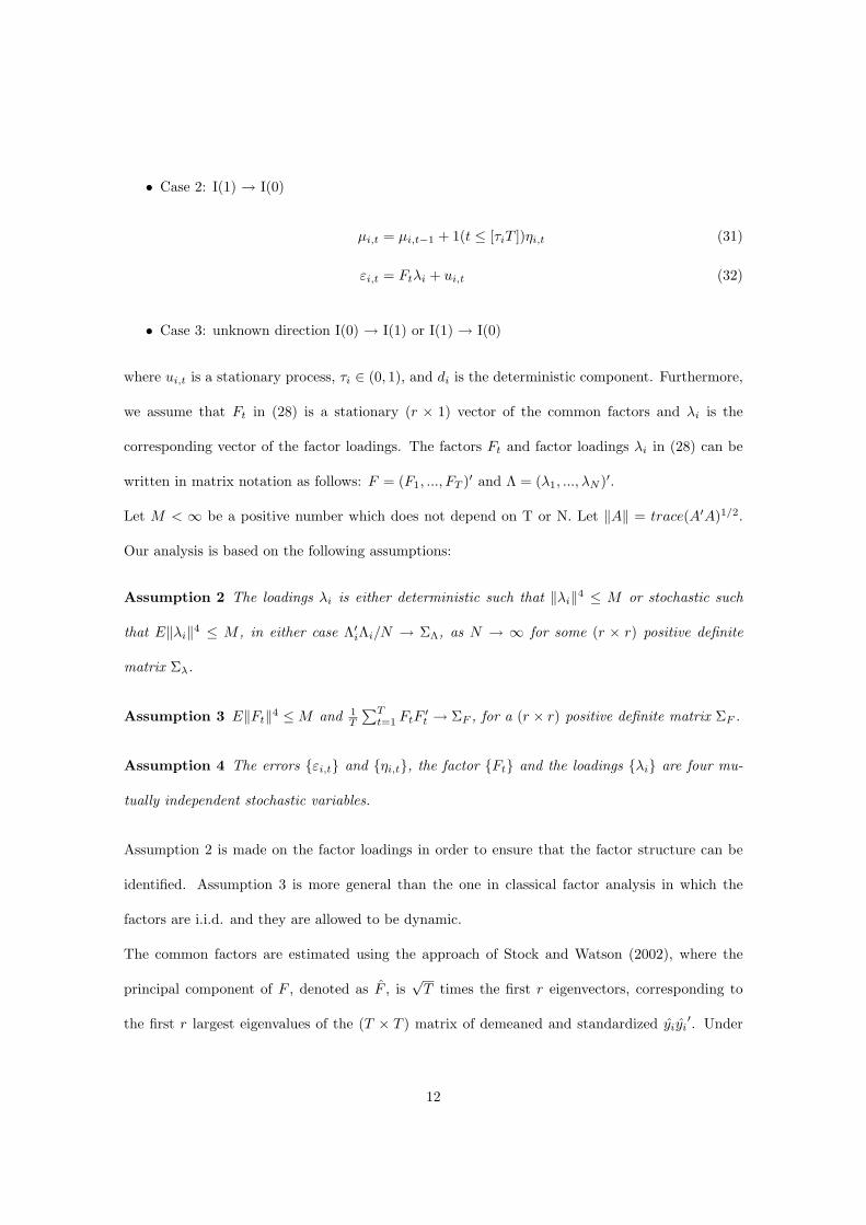
µi,t = µi,t−1 + 1(t > [τiT ])ηi,t (29)
εi,t = Ftλi + ui,t (30)
11
• Case 2: I(1) → I(0)
µi,t = µi,t−1 + 1(t ≤ [τiT ])ηi,t (31)
εi,t = Ftλi + ui,t (32)
• Case 3: unknown direction I(0) → I(1) or I(1) → I(0)
where ui,t is a stationary process, τi ∈ (0, 1), and di is the deterministic component. Furthermore,
we assume that Ft in (28) is a stationary (r × 1) vector of the common factors and λi is the
corresponding vector of the factor loadings. The factors Ft and factor loadings λi in (28) can be
written in matrix notation as follows: F = (F1, ..., FT )′ and Λ = (λ1, ..., λN )′.
Let M < ∞ be a positive number which does not depend on T or N. Let ‖A‖ = trace(A′A)1/2.
Our analysis is based on the following assumptions:
Assumption 2 The loadings λi is either deterministic such that ‖λi‖4 ≤ M or stochastic such
that E‖λi‖4 ≤ M , in either case Λ′iΛi/N → ΣΛ, as N → ∞ for some (r × r) positive definite
matrix Σλ.
Assumption 3 E‖Ft‖4 ≤ M and 1T
∑Tt=1 FtF
′t → ΣF , for a (r × r) positive definite matrix ΣF .
Assumption 4 The errors {εi,t} and {ηi,t}, the factor {Ft} and the loadings {λi} are four mu-
tually independent stochastic variables.
Assumption 2 is made on the factor loadings in order to ensure that the factor structure can be
identified. Assumption 3 is more general than the one in classical factor analysis in which the
factors are i.i.d. and they are allowed to be dynamic.
The common factors are estimated using the approach of Stock and Watson (2002), where the
principal component of F , denoted as F , is√
T times the first r eigenvectors, corresponding to
the first r largest eigenvalues of the (T × T ) matrix of demeaned and standardized yiyi′. Under
12

the normalization F F ′/T = Ir, the estimated loading matrix is Λ = F ′yi/T . Thus the estimated
residuals are defined as
zi,t = yi,t − Ftλi (33)
According to data generating process (28)-(29) and (33), one can see that for each cross section i,
the process zi,t is stationary up to and including time [τiT ] but it is nonstationary after the break,
if and only if σ2ηi > 0. Naturally the converse is true if (32) is used instead of (29).
Thus our strategy is to apply the panel test statistics presented in section 2 to the de-factored data
zi,t.
3.2 Consistency of Ft
In this section it is shown that Ft may be consistently estimated in the presence of a break.2 To
fix ideas, the case of I(0) → I(1) is considered. Model (28) may be described as follows:
yi,t = di + µi,t + Ftλi + ui,t (34)
Considering the first difference of model (34), we have
∆yi,t = ∆µi,t + ∆Ftλi + ∆ui,t (35)
In the presence of a break, ∆µi,t may result as being either stationary or nonstationary process as
shown below:
I. ∆µi,t is stationary. In this case the Bai and Ng (2002) results may be used in order to obtain
the consistency of the estimated factors.
II. ∆µi,t is nonstationary. In this case the results of Bai and Ng (2002) cannot be used since
the stationarity of the process ∆yi,t is not known a priori.
2In the case of the absence of a break, the consistency of estimated factor is obtained in Bai and Ng (2004). This
procedure can not apply in our case.
13

Let us check if ∆µi,t is stationary or not.
Theorem 3.1 Assume that τi is a uniform random variable. Then ∆µi,t is a stationary process.
Remark 5 The assumption regarding the distribution of τi in Theorem 3.1 is reasonable. Indeed,
a break may occur at any time in the sample period.
Using theorem 3.1 the procedure of Bai and Ng (2002, 2004) can be used since the process is
stationary as in I..
4 Selecting persistence across units in the panel
Following the approach of Chortareas and Kapetanios (2009), this section describes a procedure
which separates the set of the series into a group of series with a break and a group of those
without.
For each series yi,t, i = 1, . . . , N and t > 0, a binary variable is defined
Gi :=
0, σ2ηi > 0;
1, σ2ηi = 0.
(36)
G’s are collecting by defining a set of indexes iM := (i1, . . . , iM ), with M ≤ N , and the vector
GiM := (Gi1 , . . . , GiM ). The time series vector yiM ,t := (yi1,t, . . . , yiM ,t) is also introduced. We
wish to estimate the componentwise of GiM . The estimates are denoted by GiM = (Gi1 , . . . , GiM).
In order to distinguish a series with a break from one without, the panel test Ξ and modifications
of Ξ (see section 5 for the application) may be used in place of Q(T,N)j , R(T,N)
j and M(T,N)j defined
above. Analogously, the time series statistics Hj(KT,i), Hj(K∗T,i) and max{Hj(KT,i), Hj(K∗T,i)} are
denoted ξi. The statistics Ξ and ξi are conjugated if and only if Ξ is the panel statistics constructed
from the time series test ξi. In order to estimate GiM , the following algorithm is proposed:
1 Set k = 1 and i(k) := {1, . . . , N}.
14

2 Calculate the panel statistic Ξ for the set of series yi(k),t. If the test does not reject the null
hypothesis, stop and set Gi(k) = (0, . . . , 0). If the null hypothesis is rejected, go on to the
next step.
3 Set Gs = 1, where s is the index of the series associated with the maximum value of ξi which
is conjugated with Ξ. Set k = k + 1 and i(k+1) := {1, . . . , s− 1, s + 1, . . . , N}. Go to step 2.
The consistency of GiM as an estimator of GiM is defined.
Theorem 4.1 Let αT be the significance level used for the panel test Ξ. Assume that:
(i) limT→+∞
αT = 0;
(ii) limT→+∞
log(αT )
T 2√
N= 0.
Then
limT→+∞
P
(N∑
s=1
|Gs −Gs| > 0
)= 0. (37)
Let us denote the number of the series with a break as N2, where N1 := N−N2. The set of indexes
related to the series with a break is denoted as Ib, and |Ib| = N2.
Theorem 4.2 If N,T → +∞, then:
(i) Gs = 1 implies that
limT→+∞
P (Gs = 1) = 1; (38)
(ii) Gs = 0 implies the existence of a constant λ such that
limN2→+∞
limT→+∞
P
(∑
s∈Ib
|Gs −Gs| > λ
)= 0. (39)
4.1 Estimation of the break
In this subsection, a break estimation procedure is proposed for a change in persistence from I(0)
to I(1) and viceversa. Without loss of generality, the time series can be ordinated and it may be
15

assumed that Ib = {1, . . . , N2}. In order to obtain the asymptotic behavior of the break estimators,
the following assumption is made.
Assumption 6 Let µi,s+1,µi,s+2, . . . , µi,s+m, for s ∈ 0, . . . , T − 1 and m ≤ T − s be a sequence
of stationary variables. Assume that m−1∑s+m
t=s+1 µ2i,t → E[µ2
i ] for E[µ2i ] < ∞, ∀i = 1, . . . , N2.
• Case 1: I(0) → I(1).
Consider the following time series estimator:
π(0−1)i,T (τi) =
∑Tt=[Tτi]+1 µ2
i,t/(T − [Tτi])2∑[Tτi]
t=1 µ2i,t/[Tτi]
, i = 1, . . . , N2. (40)
Now, let τ(0−1)i be:
τ(0−1)i =
{argmaxτi∈(0,1)π
(0−1)i,T (τi)
}, i = 1, . . . , N2. (41)
Formula (41) provides a time series estimate of the unknown change point.
• Case 2: I(1) → I(0).
The time series estimator is now defined as follows:
π(1−0)i,T (τi) =
∑[Tτi]t=1 µ2
i,t/[Tτi]2∑Tt=[Tτi]+1 µ2
i,t/(T − [Tτi]), i = 1, . . . , N2. (42)
With respect to the estimate of the unknown change point, we have:
τ(1−0)i =
{argmaxτi∈(0,1)π
(1−0)i,T (τi)
}, i = 1, . . . , N2. (43)
The following theorem is a direct consequence of Kim (2000, Theorem 3.5) and shows the asymp-
totic properties of the estimators τ(0−1)i and τ
(1−0)i :
Theorem 7 Under the alternative hypothesis and under the Assumption 6, it results
(τ (0−1)i − τi) = (τ (1−0)
i − τi) = op(1), (44)
T (τ (0−1)i − τi) = T (τ (1−0)
i − τi) = Op(1). (45)
16

5 Monte Carlo simulation results
In this section Monte Carlo experiments are used to investigate the finite sample properties of
the panel persistence tests. Two sets of Monte Carlo experiments are considered. The first set
focuses on the model (1)-(3), where cross-section independence is assumed, while the second set
uses model (28)-(33) for dependent panels. We start the analysis by considering the empirical
rejection frequencies of the tests when the data are generated according to a change from I(0) to
I(1) as in model (1)-(3). The impact of varying the signal-to-noise ratio is investigated between
σηi = 0, 0.10, 0.50 and σεi ∼ U [0.5, 1.5] . The breakpoint is uniform distributed, τ ∼ U [0.3, 0.7].
Only the modified min panel tests are considered here for reasons of space (results for the other
panel tests are available upon request from the authors). The simulation results are performed
using 1000 Monte Carlo replications and the RNDN function of Gauss 6.0. For all the tests, we
consider N = 15, 25, 50, 100 and T = 50, 100.3 To overcome ill-conditioning arising from regression
(24), only a subset of T can be used. Following the earlier literature, we focus the analysis on the
subset [γT, (1 − γ)T )] with γ = 0.2. This choice is applied throughout this and the next section
of the paper. In Table 1 we present the moments of Kim’s (2000, 2002) and Busetti and Taylor’s
(2004) tests which are used to standardize the panel tests. Their values are computed using 50,000
replications. In Tables 2-3 we report empirical rejection frequencies for the size (H0 : σ2ηi = 0) and
power (H1 : σ2ηi > 0) of the panel tests for model (1)-(3). All the panel test statistics seem to have
good size for both small and large T, N .
Many interesting results emerge regarding the power of the tests for case 1 where I(0) → I(1)
(Table 2). The power of the tests grows as the signal-to-noise ratio rises, as is generally expected,
since the higher ση is, the stronger the random walk component. The opposite findings are found
for panel reverse tests, since a change from I(0) to I(1) is being tested.
Simulation results for the case 2 (I(1) → I(0)) are reported in Table 3. The power of the tests
3As regards the case of independent panel tests we also considered N=1.
17
grows largely for the reverse statistics and it is interesting to note that the results mimic those in
Table 2. Finally it is also should be noted that the panel tests always have a higher power than
the univariate tests. In order to take cross-section dependence into account we use the method
proposed in Stock and Watson (2002) and Bai and Ng (2004). The method consists of filtering
out the individual-specific cross-sections yit by the factor component computed using the principal
component method. We assume a single Ft ∼ N(0, 1), and Λ ∼ U [0, 1]. The number of factors
are computed using the approach of Bai and Ng (2002). Throughout the Monte Carlo simulation
analyses the number of factors are computed using the IC(3) criterion proposed by Bai and Ng
(2002) with a maximum number of three factors.
Tables 4-5 present the empirical rejection frequencies for the defactored panel tests, showing the
empirical size (H0 : σ2ηi = 0) and the power (H1 : σ2
ηi > 0). It is should be noted that the tests
have generally good size. Table 4 power reports results for a change from I(1) to I(0). The power
of the tests grows for larger values of T and N , with the exception of the reverse panel tests since
a change from I(0) to I(1) is being tested. Results of the power of tests for the case 2 (I(1) → I(0))
are reported in Table 5. The power of the tests grows considerably for the reverse tests, as would
be expected.
6 Empirical application
The new panel tests are used in the analysis of the inflation rates for a panel of 19 OECD countries.4
Quarterly CPI inflation is considered (measured as the annual change in the CPI) over the period
1972:2-2008:2. All data are taken from OECD Main Economic Indicators. Table 6 reports the
application of the modified panel persistence change tests to the aforementioned data. With
respect to the panel tests constructed under the hypothesis of cross section independence, the null4The selected countries are Australia, Austria, Belgium, Canada, Finland, France, Germany, Greece, Italy, Japan,
Luxembourg, New Zealand, Norway, Portugal, Spain, Sweden, Switzerland, United Kingdom and United States.
18

hypothesis of stationarity cannot be rejected in the case of a shift from I(0) to I(1), while it is
rejected for a change from I(1) to I(0) and also where the direction is unknown. These findings
suggest a change of persistence from I(1) to I(0) for inflation rate. However, the previous results are
valid under the assumption of cross-section independence which is rather unrealistic in empirical
economic applications. Therefore, cross-section dependence is considered thorough the use of the
factor model described in section 3.
Three factors are selected using the IC(3) criterion (from a fixed maximum of five). The estimated
factors and factor loadings are then used to obtain zi,t as in equation (33) and the panel tests are
applied to the defactored data. Results show a change in persistence from I(1) to I(0) as found in
the case of cross-section independence.
Having rejected the null hypothesis of constant persistence, the countries with a break in the
inflation rate must be identified. To this end the procedure presented in section 4 is used.5 Table
7 reports the results of the MMmin,3 test statistic (similar results are found using the other panel
tests).
We focus on the cross-section dependence case (defactored inflation rate). The statistics provided
by the procedure is 13.21 for the full set of countries, which is greater than the 5% critical value of
a standard normal distribution. Greece is the country with the maximum individual MMmin,3 and
is thus removed from the panel. The persistence test is then re-applied to the remaining countries
and the procedure continues until the panel test does not reject the null hypothesis. Table 7 reports
those countries with a break in the inflation rates. The break dates, which are estimated using
formula (42), are as follows: Greece (1998:1), Portugal (1988:4), Italy (1985:3), Japan (1978:2),
France (1985:2), Spain (1996:1), UK (1982:1) and US (1982:2). The years 1991-94 mark a transition
from a high inflation rate to a more moderate level in Greece. In 1995 the Bank of Greece adopts5Chortareas and Kapetanios (2009) use their procedure to distinguish between stationary and non stationary
series in an OECD exchange rate panel by applying Chang (2002), Im, Pesaran and Shin (2003) and Pesaran (2007)
tests.
19

a nominal exchange rate anchor as an important mechanism for disinflation (Karfakis et al., 2004)
for the first time. As a result, inflation falls from 4% in 1997 to 2.4% in 1999. In France the change
in regime of monetary policy and new wage bargaining policy in 1983 leads to a strong decline in
the average yearly growth of the CPI from nearly 11.0% before the 1985 to 2.1% afterwards. In
Italy there is also a drop in the inflation after 1985 (following the changes made to the income
policy in 1984) falling from 8.0% to 4.2% in one year. In Japan in the the mid-1970s substantial
changes in inflation are recorded, peaking in 1974 and relapsing around the end of 1970s. The
break date for Spain coincides with the year in which the government begins a monetary policy
of the inflation targeting. Similar results are found regarding the break dates for the UK and the
US. The shift in the UK occurs in the first quarter of 1982, whereas the US experiences a break
in the second quarter of 1982 (similar findings are found in Halunga et al., 2009). Various factors
contribute to the decline in UK inflation rate at the beginning of the 1980s: a restrictive monetary
policy (the government attempts to gain in credibility for their deflationary policies by convincing
economic agents that the reduction of inflation is the preeminent policy goal), a strong exchange
rate, a sharp slowdown in economic activity, and the macroeconomic discipline implied by the
Medium-Term Financial Strategy (Benati and Surico, 2008). For these reasons, the inflation rate
in the UK falls steeply from 21.0% to 4.0% in the first four years of the 1980s (see Nelson, 2003).
In the late 1970s, the US money stock is growing at an undesirably fast rate, the rate of inflation is
accelerating, and the dollar is steadily depreciating in the foreign exchange markets. Consequently
the Federal Reserve decides to take several actions, including a change in its operating procedures,
in an attempt to reverse these trends. The new procedures remain in place until the end of 1982,
when Federal Reserve Chairman Paul Volcker announces the intention to place less emphasis on
the money stock for the time being (see Anderton, 1997). As a result, the inflation falls from 10.3%
to 3.2% in 1981-1983.6
6Benati and Kapetanios (2002) show that after the Volcker disinflation
20

7 Conclusions
In this paper we present new panel tests for a change in persistence which are based on a modified
time series version of the ratio-based statistics presented in Kim (2000), Kim et al. (2002), Busetti
and Taylor (2004) and Harvey et al. (2006). The panel tests are used to test the null hypothesis
of stationarity against the alternative of a change in persistence from I(0) to I(1), from I(1) to
I(0) and when the direction is unknown. The null hypothesis may be rejected even if only one of
the cross-section units shows a change in persistence since the null hypothesis assumes no change
in persistence in any of the cross-section units. Therefore, the panel tests are sensitive to the
selection of the cross-section units in the panel. Hence, following Chortareas and Kapetanios
(2009), a procedure to identify the series which undergo changes in persistence is used.
Two sets of panel tests are proposed here. The first set is assigned to cross-sectionally independent
panels. The asymptotic distributions of these tests are derived and are shown to be normally
distributed. The second set uses the hypothesis of cross-section dependence and defactored data
are then applied. On conducting a Monte Carlo experiment considerable increases in power with
respect to the univariate changes in persistence tests are found. The new tests are applied to
quarterly inflation rate of a panel of 19 OECD countries over the period 1972:2-2008:2. The results
show evidence in favor of a change in persistence from I(1) to I(0) for a set of these countries.
ACKNOWLEDGEMENTS
The authors would like to thank David Hendry, Chihwa Kao, Oliver Linton and other partici-
pants at the First International Conference in Memory of Carlo Giannini, “Recent Development in
Econometric Methodology”, University of Bergamo, 25-26 January 2008, for helpful comments and
suggestions. The authors also thank Robert Kunst and other seminar participants at University of
Vienna, 6 February 2008, and Stephen Pollock, Wojciech Charemza, Panicos Demetriades, Qiang
21

Zhang, Francesco Moscone and other seminar participants at University of Leicester, 1 October
2008.
REFERENCES
Alogoskoufis GS, Smith R. 1991. The Phillips Curve, the Persistence of Inflation, and the Lucas
Critique: Evidence from Exchange-Rate Regimes. American Economic Review 81 : 1254-75.
Anderton R. 1997. Did the underlying behavior of inflation change in the 1980s? A study of 17
countries. Review of World Economics 133 : 22-38.
Andrews DWK. 1993. Tests for parameter instability and structural change with unknown change
point. Econometrica 61 : 821-856.
Andrews DWK, Ploberger W. 1994. Optimal tests when a nuisance parameter is present only
under the alternative. Econometrica 62 : 1383-1414.
Bai J. 2003. Inferential theory for factor models of large dimensions. Econometrica 71 : 135-171.
Bai J, Ng S. 2002. Determining the number of factors in approximate factor models. Econometrica
70 : 191-221.
Bai J, Ng S. 2004. A PANIC attack on unit roots and cointegration. Econometrica 72 : 1127-1177.
Barsky RB. 1987. The Fisher Hypothesis and the Forecastability and Persistence of Inflation.
Journal of Monetary Economics 19 : 324.
Benati L, Surico P. 2008. Evolving U.S. Monetary Policy and The Decline of Inflation Predictabil-
ity. Journal of the European Economic Association 6 : 634-646.
Breitung J, Pesaran MH. 2008. Unit Roots and Cointegration in Panels. In The Econometrics of
Panel Data, Matyas L, Sevestre P (eds). Springer: Berlin.
Busetti F, Taylor AMR. 2004. Tests of stationarity against a change in persistence. Journal of
Econometrics 123 : 33-66.
Clark TE. 2006. Disaggregate evidence on the persistence of consumer price inflation. Journal of
Applied Econometrics 21 : 563-587.
22

Chang Y. 2002. Nonlinear IV unit root tests in panels with cross-sectional dependency. Journal
of Econometrics 110 : 261292.
Chortareas G, Kapetanios G. 2009. Getting PPP right: Identifying mean-reverting real exchange
rates in panels. Journal of Banking & Finance 33 : 390-404.
Costantini M, Gutierrez L. 2007. Simple panel unit root tests to detect change in persistence.
Economics Letters 96 : 363-368.
Costantini M, Lupi C. 2007. An analysis of inflation and interest rates. New panel unit root results
in the presence of structural breaks. Economics Letters 95 : 408-414.
Davies RB. 1977. Hypothesis testing when a nuisance parameter is present under the alternative.
Biometrika 64 : 247-254.
Emery KM. 1994. Inflation persistence and Fisher effects: evidence of a regime change. Journal
of Economics and Business 46 : 141152.
Halunga AG, Osborn DR, Sensier M. 2009. Changes in the order of integration of US and UK
inflation. Economics Letters 102 : 30-32.
Hansen BE. 1991. Testing for structural change of unknown form in models with nonstationary
regressors, Department of Economics, University of Rochester, Mimeo.
Harvey DI, Leybourne SJ, Taylor RAM. 2006. Modified tests for a change in persistence. Journal
of Econometrics 134 : 441469.
Hawkins DL. 1987. A test for a change point in a parametric model based on a maximum Wald-type
statistic. Sankhya 49 : 368-376.
Im KS, Pesaran MH, Shin Y. 2003. Testing for unit roots in heterogeneous panels. Journal of
Econometrics 115 : 5374.
Karfakis C, Moschos D, Sidiropoulos M. 2004. Capital Mobility and Inflation Persistence: Theory
and Evidence from Greece. International Journal of Finance and Economics 9 : 125-133.
23

Kim JY. 2000. Detection of change in persistence of a linear time series. Journal of Econometrics
95 : 97-116.
Kim JY, Franch, JB, Amador RB. 2002. Corrigendum to “Detection of change in persistence of a
linear time series”. Journal of Econometrics 109 : 389-392.
Kim HJ, Siegmund D. 1989. The likelihood ratio test for a change point in a simple linear regression.
Biometrika 76 : 409-423.
Nelson E. 2003. UK monetary policy 1972-97: a guide using Taylor rules. In Central Banking,
Monetary Theory and Practice: Essays in Honour of Charles Goodhart, P. Mizen (ed.) Chel-
tenham, Edward Elgar.
Pesaran MH. 2007. A simple panel unit root test in the presence of cross section dependence.
Journal of Applied Econometrics 22 : 265-312.
Phillips P. 1987. Time Series Regression with a Unit Root. Econometrica 55 : 277-301.
Phillips PCB, Perron P. 1988. Testing for a unit root in time series regression. Biometrika 75 :
335-346.
Phillips PCB, Solo V. 1992. Asymptotics for Linear Processes. Annals of Statistics 20 : 971-1001.
Stock JH, Watson, MW. 2002. Macroeconomic forecasting using diffusion indices. Journal of
Business and Economic Statistics 20 : 147-162.
24

Appendix A: Mathematical Proofs
Proof of Theorem 2.1. By Theorem 3.1 in Kim (2000), it results
limT→+∞
KT,i(τi) =(1− τi)−2
∫ 1
τiBi(r − τi)2dr
τ−2i
∫ τi
0Bi(r)2dr
,
where {Bi}+∞i=1 is a sequence of standard brownian bridges that are independent and identically
distributed. Furthermore, by the hypotheses stated in Assumption 1, we have that
limT→+∞
E[Hj
((T − [Tτi])−2
[Tτi]−2
∑Tt=[Tτi]+1 S
(1)i,t (τi)2
∑[Tτi]t=1 S
(0)i,t (τi)2
)]= µ
(Q)j , i = 1, . . . , N, j = 1, 2, 3;
limT→+∞
√√√√V[Hj
((T − [Tτi])−2
[Tτi]−2
∑Tt=[Tτi]+1 S
(1)i,t (τi)2
∑[Tτi]t=1 S
(0)i,t (τi)2
)]= σ
(Q)j , i = 1, . . . , N, j = 1, 2, 3,
with
µ(Q)j := E
[Hj
((1− τi)−2
∫ 1
τiBi(r − τi)2dr
τ−2i
∫ τi
0Bi(r)2dr
)], i = 1, . . . , N ; (A.1)
and
σ(Q)j :=
√√√√V[Hj
((1− τi)−2
∫ 1
τiBi(r − τi)2dr
τ−2i
∫ τi
0Bi(r)2dr
) ], i = 1, . . . , N. (A.2)
The continuous mapping theorem and the continuity of the functionals imply
limT→+∞
Hj
(KT,i(τi)
)= Hj
((1− τi)−2
∫ 1
τiBi(r − τi)2dr
τ−2i
∫ τi
0Bi(r)2dr
).
The Central Limit Theorem guarantees that
limN→+∞
1√Nσ
(Q)j
·N∑
i=1
[Hj
((1− τi)−2
∫ 1
τiBi(r − τi)2dr
Nτ−2i
∫ τi
0Bi(r)2dr
)− µ
(Q)j
]∼ N(0, 1),
and the Theorem is completely proved.
Proof of Theorem 2.2. By Theorem 3.1 in Busetti and Taylor (2004), it results
limT→+∞
K∗T,i =τ−2i
∫ τi
0[V ∗∗∗
i (r)]2dr
(1− τi)−2∫ 1
τi[V ∗∗
i (r)]2dr,
where
V ∗∗i (r) = Vi(r)− Vi(τi)− (r − τi)(1− τi)−1(Vi(1)− Vi(τi))
25

V ∗∗∗i (r) = Vi(r)− rτ−1
i Vi(τi)
and
Vi(r) = W0(r) + c
{∫ min{r,τi}
0
Wc(s)ds + 1(r > τi)[(r − τi)Wc(τi)]
},
where W0 and Wc are independent standard Wiener processes. Hypotheses stated in Assumption
1 imply
limT→+∞
E[Hj
([Tτi]−2
∑[Tτi]t=1 S
(0)i,t (τi)2
(T − [Tτi])−2∑T
t=[Tτi]+1 S(1)i,t (τi)2
)]= µ
(R)j , i = 1, . . . , N, j = 1, 2, 3;
limT→+∞
√√√√V[Hj
([Tτi]−2
∑[Tτi]t=1 S
(0)i,t (τi)2
(T − [Tτi])−2∑T
t=[Tτi]+1 S(1)i,t (τi)2
)]= σ
(R)j , i = 1, . . . , N, j = 1, 2, 3,
where
µ(R)j := E
[Hj
(τi−2
∫ τi
0[V ∗∗∗
i (r)]2dr
(1− τi)−2∫ 1
τi[V ∗∗
i (r)]2dr
)], i = 1, . . . , N, j = 1, 2, 3, (A.3)
and
σ(R)j =
√√√√V[Hj
(τi−2
∫ τi
0[V ∗∗∗
i (r)]2dr
(1− τi)−2∫ 1
τi[V ∗∗
i (r)]2dr
) ], i = 1, . . . , N, j = 1, 2, 3. (A.4)
The continuous mapping theorem and the continuity of the functionals imply
limT→+∞
Hj
(K∗T,i(τi)
)= Hj
(τ−2i
∫ τi
0[V ∗∗∗
i (r)]2dr
(1− τi)−2∫ 1
τi[V ∗∗
i (r)]2dr
).
By Central Limit Theorem we have
limN→+∞
1√Nσ
(R)j
·N∑
i=1
[Hj
(τ−2i
∫ τi
0[V ∗∗∗
i (r)]2dr
(1− τi)−2∫ 1
τi[V ∗∗
i (r)]2dr
)− µ
(R)j
]∼ N(0, 1),
and the Theorem is completely proved.
Proof of Theorem 2.3. It is a direct consequence of the Central Limit Theorem.
26
Proof of Theorem 3.1. By (29) we have
∆µi,t = 1(t > [τiT ])ηi,t. (A.5)
The break can be observed in a specified time of the sample period. By assumption, we have that
τi is an uniform random variable in (0, 1). In our model we consider breaks in [τiT ]. Therefore,
we do not lose of generality by assuming that τi is discrete, and takes uniformly values in the set
Γ := {j/T}j=0,...,T−1. This assumption is made throughout the proof. The distribution of ∆µi,t
can be obtained using all the possible realizations of τi and applying standard stochastic calculus
techniques. For each x ∈ R, we have
P (∆µi,t ≤ x) =T−1∑
j=0
P (∆µi,t ≤ x∣∣∣ τi =
j
T) · P (τi =
j
T) =
=1T·
T−1∑
j=0
P (∆µ(j)i,t ≤ x), (A.6)
where
∆µ(j)i,t =
0, if t ≤ j;
ηi,t, if t > j.(A.7)
For each j = 0, . . . , T − 1, the definition of ηi,t implies that ∆µ(j)i,t is a stationary process with zero
mean and finite variance (independent of t). Moreover, the expected value and variance of ∆µi,t can
be obtained as a linear combination of expected values and variances of the ∆µ(j)i,t , j = 0, . . . , T −1
using equation (A.6). Therefore, ∆µi,t has zero mean and finite variance (independent of t), and
the theorem is completely proved.
Proof of Theorem 4.1 First of all, it should be noted that the statistics Ξ is a one-sided test.
Denote the αT -critical value of the test Ξ as cT .
The algorithm does not stop as long as there exist any series with break in yi(k),t. The series with
break are removed from the panel until no series with break are not contained in the set of series.
Thus the following three statements are needed to be proved.
27

(I) Fixed N , then
limT→+∞
P (Ξ > cT ) = 1,
if Ξ has been constructed on the set of series yi(k),t, containing at least one series with break.
(II) Fixed N , then
limT→+∞
P (Ξ > cT ) = 0,
if Ξ has been constructed on the set of series yi(k),t, where no series of yi(k),t contains a break.
(III) If yi(k),t contains a series with break, then the maximum test ξi, conjugated with Ξ, corre-
sponds to a series with a break, with probability approaching to 1.
We first prove (I). Under the alternative hypothesis, Kim (2000) shows that ξi ∼ Op(1) or ξi ∼
Op(T 2), depending on the considered model or time series statistics. This implies that Ξ ∼ Op(√
N)
or Ξ ∼ Op(T 2√
N), even if yi(k),t contains only one series with break. Since√
N → +∞ as well
as T 2√
N → +∞, we obtain that all the panel statistics denoted by Ξ are consistent, for each N ,
even if yi(k),t contains only one series with break. We now need to prove that
cT
T 2√
N→ 0
to show the validity of (I). This is a direct consequence of the hypotheses and the convergence of
ξi to a functional of Brownian Motion, as T → +∞, following Chortareas and Kapetanios (2009).
We now show (II). If yi(k),t contains no series with break, then Ξ = Op(1). In this case αT → 0
which implies that cT → +∞, and (II) holds.
To complete the proof it should be noted that, if Gm = 1 and Gn = 0, then
P (ξm > ξn) → 1,
for each n,m. Indeed, ξm → +∞ and ξn = Op(1), and then (III) holds true.
Proof of Theorem 4.2 The proof is a direct consequence of Theorem 4.1 and Theorem 2 in
Chortareas and Kapetanios (2009).
28

Table 1: Simulated moments for individual Kim(2000, 2002) and Busetti and Taylor tests (2004)
T Q1 Q2 Q3 R1 R2 R3 M1 M2 M3
Mean - drift case
50 1.817 1.608 6.173 1.836 1.624 6.204 2.783 2.632 9.214
100 1.803 1.566 6.386 1.803 1.564 6.391 2.749 2.545 9.436
500 1.800 1.537 6.788 1.779 1.506 6.660 2.741 2.478 9.868
Std. deviation - drift case
50 1.580 2.282 5.856 1.586 2.370 6.003 1.737 2.903 6.874
100 1.548 2.178 5.841 1.526 2.106 5.728 1.669 2.644 6.590
500 1.528 2.170 6.041 1.503 1.980 5.701 1.667 2.562 6.318
29

Table 2: Rejection frequencies min Panel Tests When the Model Does Not Allow for Cross SectionalDependence. I(0) → I(1). Intercept case.
T N ση MQmin,1 MQmin,2 MQmin,3 MRmin,1 MRmin,2 MRmin,3 MMmin,1 MMmin,2 MMmin,3
50 1 0 0.060 0.054 0.063 0.058 0.045 0.058 0.054 0.049 0.06450 1 0.1 0.088 0.080 0.027 0.858 0.857 0.828 0.836 0.832 0.80550 1 0.5 0.692 0.686 0.650 0.515 0.507 0.426 0.770 0.774 0.74550 15 0 0.063 0.062 0.056 0.062 0.061 0.075 0.052 0.054 0.05850 15 0.1 0.699 0.736 0.495 1.000 1.000 1.000 1.000 1.000 1.00050 15 0.5 1.000 1.000 1.000 0.984 0.984 0.884 1.000 1.000 1.00050 25 0 0.072 0.067 0.065 0.058 0.054 0.065 0.070 0.067 0.07450 25 0.1 0.905 0.931 0.635 1.000 1.000 1.000 1.000 1.000 1.00050 25 0.5 1.000 1.000 1.000 0.999 0.999 0.934 1.000 1.000 1.00050 50 0 0.072 0.071 0.074 0.058 0.060 0.059 0.068 0.065 0.06750 50 0.1 0.984 0.996 0.826 1.000 1.000 1.000 1.000 1.000 1.00050 50 0.5 1.000 1.000 1.000 1.000 1.000 0.988 1.000 1.000 1.00050 100 0 0.059 0.063 0.062 0.051 0.049 0.049 0.051 0.055 0.05550 100 0.1 0.999 1.000 0.930 1.000 1.000 1.000 1.000 1.000 1.00050 100 0.5 1.000 1.000 1.000 1.000 1.000 1.000 1.000 1.000 1.000
100 1 0 0.052 0.046 0.049 0.073 0.067 0.073 0.072 0.064 0.071100 1 0.1 0.489 0.490 0.494 0.636 0.621 0.472 0.711 0.702 0.639100 1 0.5 0.882 0.881 0.900 0.143 0.129 0.038 0.857 0.858 0.871100 15 0 0.055 0.058 0.051 0.064 0.073 0.071 0.053 0.054 0.061100 15 0.1 0.987 0.989 0.948 1.000 1.000 1.000 1.000 1.000 1.000100 15 0.5 1.000 1.000 1.000 0.983 0.986 0.840 1.000 1.000 1.000100 25 0 0.061 0.063 0.064 0.057 0.055 0.045 0.062 0.061 0.058100 25 0.1 1.000 1.000 0.998 1.000 1.000 1.000 1.000 1.000 1.000100 25 0.5 1.000 1.000 1.000 0.988 0.992 0.768 1.000 1.000 1.000100 50 0 0.061 0.061 0.056 0.052 0.047 0.053 0.053 0.056 0.053100 50 0.1 1.000 1.000 1.000 1.000 1.000 1.000 1.000 1.000 1.000100 50 0.5 1.000 1.000 1.000 1.000 1.000 0.984 1.000 1.000 1.000100 100 0 0.060 0.059 0.060 0.066 0.071 0.059 0.061 0.062 0.052100 100 0.1 1.000 1.000 1.000 1.000 1.000 1.000 1.000 1.000 1.000100 100 0.5 1.000 1.000 1.000 1.000 1.000 0.973 1.000 1.000 1.000
Notes: Empirical sizes corresponding to a 5% nominal size.
30

Table 3: Rejection frequencies min Panel Tests When the Model Does Not Allow for Cross SectionalDependence. I(1) → I(0). Intercept case.
T N ση MQmin,1 MQmin,2 MQmin,3 MRmin,1 MRmin,2 MRmin,3 MMmin,1 MMmin,2 MMmin,3
50 1 0 0.064 0.050 0.061 0.059 0.053 0.062 0.054 0.049 0.06450 1 0.1 0.861 0.857 0.829 0.087 0.079 0.027 0.836 0.832 0.80550 1 0.5 0.517 0.510 0.427 0.687 0.680 0.648 0.770 0.774 0.74550 15 0 0.068 0.069 0.080 0.057 0.057 0.052 0.052 0.054 0.05850 15 0.1 1.000 1.000 1.000 0.693 0.723 0.487 1.000 1.000 1.00050 15 0.5 0.984 0.984 0.886 1.000 1.000 1.000 1.000 1.000 1.00050 25 0 0.067 0.059 0.069 0.066 0.057 0.057 0.070 0.067 0.07450 25 0.1 1.000 1.000 1.000 0.903 0.923 0.621 1.000 1.000 1.00050 25 0.5 0.999 0.999 0.936 1.000 1.000 1.000 1.000 1.000 1.00050 50 0 0.064 0.068 0.070 0.063 0.060 0.065 0.068 0.065 0.06750 50 0.1 1.000 1.000 1.000 0.980 0.994 0.815 1.000 1.000 1.00050 50 0.5 1.000 1.000 0.990 1.000 1.000 0.988 1.000 1.000 1.00050 100 0 0.059 0.060 0.058 0.050 0.048 0.054 0.051 0.055 0.05550 100 0.1 1.000 1.000 1.000 0.998 0.999 0.922 1.000 1.000 1.00050 100 0.5 1.000 1.000 1.000 1.000 1.000 1.000 1.000 1.000 1.000
100 1 0 0.071 0.063 0.072 0.052 0.049 0.049 0.072 0.064 0.071100 1 0.1 0.633 0.616 0.467 0.491 0.496 0.496 0.711 0.702 0.639100 1 0.5 0.141 0.127 0.036 0.884 0.883 0.900 0.857 0.858 0.871100 15 0 0.064 0.066 0.069 0.058 0.060 0.053 0.053 0.054 0.061100 15 0.1 1.000 1.000 1.000 0.987 0.989 0.950 1.000 1.000 1.000100 15 0.5 0.983 0.987 0.837 1.000 1.000 1.000 1.000 1.000 1.000100 25 0 0.054 0.051 0.044 0.064 0.070 0.065 0.062 0.061 0.058100 25 0.1 1.000 1.000 1.000 1.000 1.000 1.000 0.998 1.000 1.000100 25 0.5 0.998 0.992 0.767 1.000 1.000 1.000 1.000 1.000 1.000100 50 0 0.048 0.044 0.052 0.062 0.064 0.056 0.053 0.056 0.053100 50 0.1 1.000 1.000 1.000 1.000 1.000 1.000 1.000 1.000 1.000100 50 0.5 1.000 1.000 0.984 1.000 1.000 1.000 1.000 1.000 1.000100 100 0 0.063 0.064 0.056 0.062 0.069 0.063 0.061 0.062 0.052100 100 0.1 1.000 1.000 1.000 1.000 1.000 1.000 1.000 1.000 1.000100 100 0.5 1.000 1.000 0.973 1.000 1.000 1.000 1.000 1.000 1.000
Notes: Empirical sizes corresponding to a 5% nominal size.
31

Table 4: Rejection frequencies of Defactored Modified Min Panel Tests. I(0) → I(1). Interceptcase.
T N ση MQmin,1 MQmin,2 MQmin,3 MRmin,1 MRmin,2 MRmin,3 MMmin,1 MMmin,2 MMmin,3
50 15 0 0.065 0.065 0.065 0.063 0.066 0.070 0.068 0.071 0.07450 15 0.1 0.446 0.471 0.284 0.952 0.950 0.942 0.943 0.947 0.92950 15 0.5 0.999 0.999 0.999 0.885 0.889 0.613 1.000 1.000 1.00050 25 0 0.067 0.071 0.068 0.073 0.072 0.063 0.066 0.070 0.07350 25 0.1 0.603 0.648 0.378 0.997 0.997 0.992 0.993 0.994 0.98850 25 0.5 1.000 1.000 1.000 0.967 0.973 0.711 1.000 1.000 1.00050 50 0 0.068 0.072 0.075 0.074 0.078 0.065 0.075 0.075 0.07450 50 0.1 0.859 0.899 0.571 1.000 1.000 1.000 1.000 1.000 1.00050 50 0.5 1.000 1.000 1.000 0.996 0.997 0.785 1.000 1.000 1.00050 100 0 0.065 0.071 0.071 0.067 0.071 0.060 0.076 0.070 0.07350 100 0.1 0.959 0.980 0.727 1.000 1.000 1.000 1.000 1.000 1.00050 100 0.5 1.000 1.000 1.000 1.000 1.000 0.965 1.000 1.000 1.000
100 15 0 0.073 0.065 0.071 0.068 0.070 0.074 0.076 0.073 0.073100 15 0.1 0.925 0.930 0.838 0.992 0.993 0.968 0.997 0.997 0.992100 15 0.5 1.000 1.000 1.000 0.931 0.946 0.619 1.000 1.000 1.000100 25 0 0.070 0.069 0.070 0.068 0.068 0.060 0.066 0.070 0.063100 25 0.1 0.983 0.989 0.962 0.999 0.998 0.989 0.999 1.000 0.999100 25 0.5 1.000 1.000 1.000 0.972 0.977 0.657 1.000 1.000 1.000100 50 0 0.068 0.063 0.073 0.068 0.071 0.062 0.060 0.060 0.058100 50 0.1 1.000 1.000 0.997 1.000 1.000 1.000 1.000 1.000 1.000100 50 0.5 1.000 1.000 1.000 0.999 0.999 0.856 1.000 1.000 1.000100 100 0 0.058 0.051 0.050 0.066 0.067 0.065 0.064 0.067 0.062100 100 0.1 1.000 1.000 1.000 1.000 1.000 1.000 1.000 1.000 1.000100 100 0.5 1.000 1.000 1.000 1.000 1.000 0.932 1.000 1.000 1.000
Notes:Empirical sizes corresponding to a 5% nominal size.
32

Table 5: Rejection frequencies of Defactored Modified Min Panel Tests. I(1) → I(0). Interceptcase.
T N ση MQmin,1 MQmin,2 MQmin,3 MRmin,1 MRmin,2 MRmin,3 MMmin,1 MMmin,2 MMmin,3
50 15 0 0.065 0.068 0.069 0.072 0.073 0.074 0.068 0.073 0.07550 15 0.1 0.969 0.965 0.954 0.373 0.404 0.293 0.950 0.950 0.93850 15 0.5 0.938 0.937 0.676 0.998 0.998 0.999 1.000 1.000 1.00050 25 0 0.076 0.072 0.068 0.078 0.074 0.072 0.068 0.075 0.07550 25 0.1 0.999 0.999 0.998 0.537 0.594 0.317 0.996 0.996 0.99250 25 0.5 0.983 0.982 0.793 1.000 1.000 1.000 1.000 1.000 1.00050 50 0 0.071 0.073 0.074 0.075 0.075 0.068 0.073 0.073 0.07150 50 0.1 1.000 1.000 1.000 0.769 0.843 0.741 1.000 1.000 1.00050 50 0.5 0.999 1.000 0.888 1.000 1.000 1.000 1.000 1.000 1.00050 100 0 0.071 0.073 0.070 0.070 0.064 0.048 0.074 0.067 0.05950 100 0.1 1.000 1.000 1.000 0.927 0.961 0.640 1.000 1.000 1.00050 100 0.5 1.000 1.000 0.991 1.000 1.000 1.000 1.000 1.000 1.000
100 15 0 0.073 0.078 0.073 0.075 0.074 0.068 0.074 0.077 0.074100 15 0.1 0.991 0.993 0.973 0.924 0.931 0.847 0.996 0.996 0.991100 15 0.5 0.951 0.955 0.657 1.000 1.000 1.000 1.000 1.000 1.000100 25 0 0.057 0.061 0.055 0.068 0.067 0.067 0.061 0.061 0.056100 25 0.1 0.997 0.998 0.992 0.984 0.989 0.961 0.999 1.000 1.000100 25 0.5 0.977 0.983 0.714 1.000 1.000 1.000 1.000 1.000 1.000100 50 0 0.077 0.068 0.072 0.068 0.064 0.065 0.059 0.059 0.061100 50 0.1 1.000 1.000 1.000 1.000 1.000 0.997 1.000 1.000 1.000100 50 0.5 0.999 0.999 0.893 1.000 1.000 1.000 1.000 1.000 1.000100 100 0 0.064 0.069 0.062 0.064 0.067 0.063 0.069 0.066 0.060100 100 0.1 1.000 1.000 1.000 1.000 1.000 1.000 1.000 1.000 1.000100 100 0.5 1.000 1.000 0.965 1.000 1.000 1.000 1.000 1.000 1.000
Notes:Empirical sizes corresponding to a 5% nominal size.
33
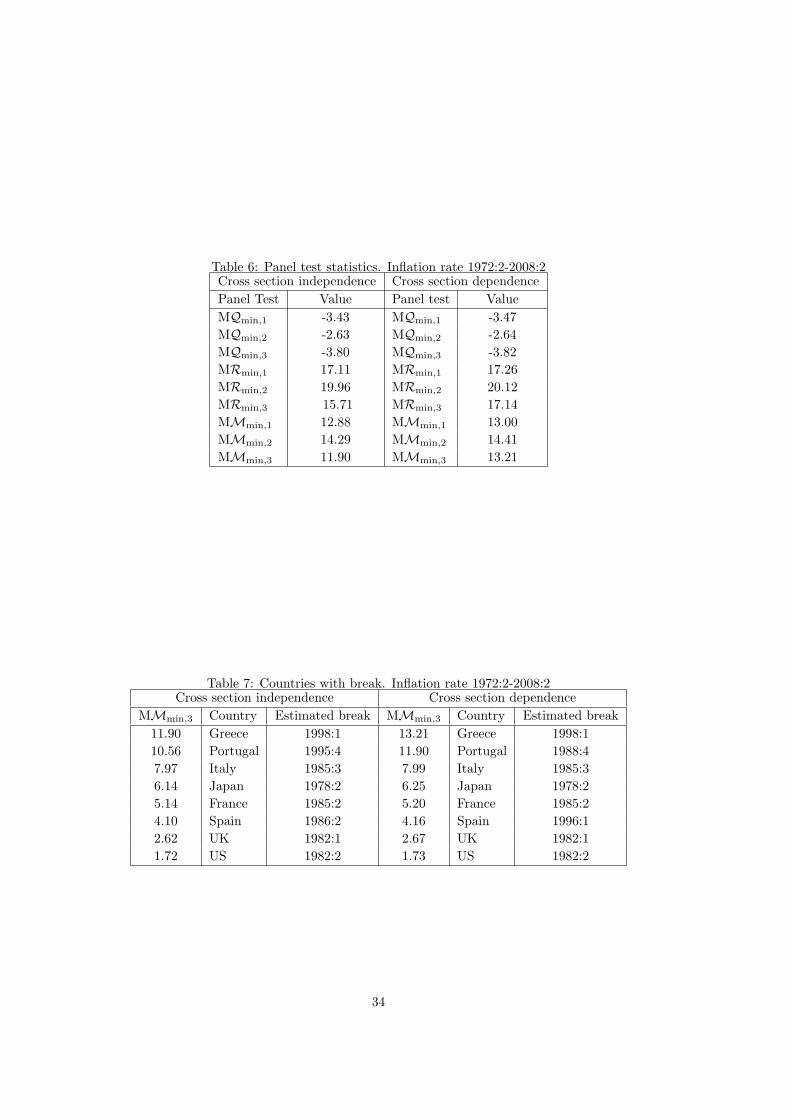
Table 6: Panel test statistics. Inflation rate 1972:2-2008:2Cross section independence Cross section dependencePanel Test Value Panel test ValueMQmin,1 -3.43 MQmin,1 -3.47MQmin,2 -2.63 MQmin,2 -2.64MQmin,3 -3.80 MQmin,3 -3.82MRmin,1 17.11 MRmin,1 17.26MRmin,2 19.96 MRmin,2 20.12MRmin,3 15.71 MRmin,3 17.14MMmin,1 12.88 MMmin,1 13.00MMmin,2 14.29 MMmin,2 14.41MMmin,3 11.90 MMmin,3 13.21
Table 7: Countries with break. Inflation rate 1972:2-2008:2Cross section independence Cross section dependence
MMmin,3 Country Estimated break MMmin,3 Country Estimated break11.90 Greece 1998:1 13.21 Greece 1998:110.56 Portugal 1995:4 11.90 Portugal 1988:47.97 Italy 1985:3 7.99 Italy 1985:36.14 Japan 1978:2 6.25 Japan 1978:25.14 France 1985:2 5.20 France 1985:24.10 Spain 1986:2 4.16 Spain 1996:12.62 UK 1982:1 2.67 UK 1982:11.72 US 1982:2 1.73 US 1982:2
34