Coordination, Fair Treatment and Inflation Persistence*

by

John C. Driscoll Federal Reserve Board

Mail Stop 75 20th and Constitution Avenue, NW

Washington DC 20551 email:John_Driscoll@alum.mit.edu

homepage: http://www.johncdriscoll.net and

Steinar Holden University of Oslo and Norges Bank

Department of Economics, University of Oslo Box 1095 Blindern, 0317 Oslo, Norway

email: steinar.holden@econ.uio.no homepage: http://folk.uio.no/~sholden/

First draft: 28 March 2001

This version: 10 December 2002

Abstract

Most wage-contracting models with rational expectations fail to replicate the persistence in inflation observed in the data. We argue that coordination problems and multiple equilibria are the keys to explaining inflation persistence. We develop a wage-contracting model in which workers are concerned about being treated fairly. This model generates a continuum of equilibria (consistent with a range for the rate of unemployment), where workers want to match the wage set by other workers. If workers’ expectations are based on the past behavior of wage growth, these beliefs will be self-fulfilling and thus rational. Based on quarterly U.S. data over the period 1955-2000, we find evidence that inflation is more persistent between unemployment rates of 4.7 and 6.5 percent, than outside these bounds, as predicted by our model. Keywords: Inflation persistence, coordination problems, adaptive expectations. JEL Classification numbers: E31, E3, E5. * The paper has benefited from comments by V. Bhaskar, Jeff Fuhrer, Greg Mankiw, Ian McDonald, Ragnar Nymoen, Andrew Oswald, and participants at seminars at Boston University, the Boston Fed, the University of Oregon, the Kiel Institute, the University of Oslo, Rutgers University and NBER Conferences on Macroeconomics and Individual Decision Making and on Monetary Economics. Steinar Holden is grateful to the NBER for its hospitality when most of this paper was written. The opinions expressed in this paper are those of the authors and do not necessarily reflect the views of the Board of Governors of the Federal Reserve System

1

1 Introduction In recent years the short run aggregate supply curve has been the subject of renewed

interest. Much of the theoretical literature has converged on a Taylor (1980) and Calvo

(1983) type relationship, where nominal wage or price stickiness is combined with the

assumption of rational expectations; the result is sometimes referred to as the New

Keynesian Phillips curve. However, as has been pointed out by Fuhrer and Moore (1995)

and more recently by Taylor (1999) and Mankiw (2000), these models run into serious

problems when confronted with data: the models predict stickiness in prices, but not in

inflation, and are thus unable to explain the inertia of actual inflation. Furthermore, as

shown by Ball (1994), the models predict that anticipated disinflation is expansionary,

which seems inconsistent with the experiences of many countries in the 1980s and 90s.

Perhaps most intriguingly, Mankiw (2001) has observed that the models predict that a

contractionary monetary shock causing a delayed and gradual decline in inflation should

cause unemployment to fall during the transition, in stark contrast to the received wisdom

of the effect of monetary contractions.

In short, macroeconomists are faced with the puzzle that the standard formulation

of the short run aggregate supply curve seems to be an empirical failure. The search for a

model that is both theoretically and empirically satisfying has led to a number of different

suggestions, including among others near-rational expectation formation (Roberts, 1998,

and Ball, 2000), slowly diffusing information (Mankiw and Reis, 2001), and on replacing

the output gap with marginal costs (Gali and Gertler, 1999, and Sbordone, 2002; for a

critique, see Bårdsen, Jansen and Nymoen, 2002). However, all these suggestions have

their weaknesses, and it seems fair to say that the profession is still looking for a

satisfying alternative.

2

In this paper, we propose a new explanation for inflation persistence, based on

coordination problems arising from the existence of a range of equilibrium output levels.

In most existing price (or wage) setting models, while comparisons with other price

setters are important to the individual price setter, these comparisons generate persistence

in the level, but not the growth rate, of prices. We show that the existence of a range of

equilibria opens up for a new vehicle of persistence that may also affect growth rates.

With a range of equilibria, agents cannot deduce logically the future actions of other price

setters from the assumption that they behave rationally. In this situation we argue that the

past behavior of the price setters takes a prominent position as a focal point. More

specifically, the past behavior of the price setters may work as an equilibrium selection

device: among all the actions consistent with a possible equilibrium, agents expect other

agents to play as they have played in the past.

The key requirement for these features is thus the existence of a range of

equilibria for the economy. In the literature, a number of mechanisms generating a range

of equilibria have been proposed; see the survey of theories and evidence in McDonald

(1995). We focus on only one, following Bhaskar (1990). Specifically, we assume that

workers are concerned about fair treatment, in the sense that they care disproportionately

more about being paid less than other workers than they do about being paid more than

other workers. When this assumption is incorporated in a standard wage bargaining

model, the result is a continuum of rational expectations equilibria, in the form of a range

of wage growth rates for which each wage setter will aim for the same wage growth as

set by the others. Combining wage setting with the price setting behavior of firms, the

range of possible rates of wage growth transforms into a range of equilibrium rates of

3

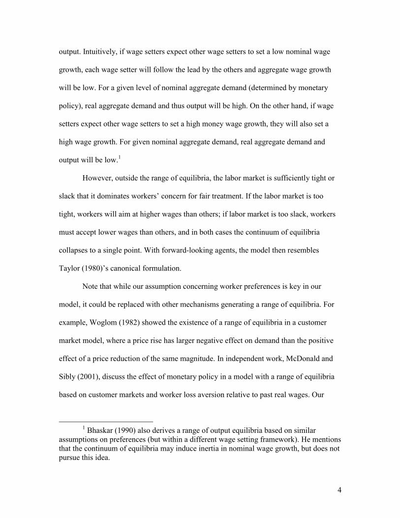
output. Intuitively, if wage setters expect other wage setters to set a low nominal wage

growth, each wage setter will follow the lead by the others and aggregate wage growth

will be low. For a given level of nominal aggregate demand (determined by monetary

policy), real aggregate demand and thus output will be high. On the other hand, if wage

setters expect other wage setters to set a high money wage growth, they will also set a

high wage growth. For given nominal aggregate demand, real aggregate demand and

output will be low.1

However, outside the range of equilibria, the labor market is sufficiently tight or

slack that it dominates workers’ concern for fair treatment. If the labor market is too

tight, workers will aim at higher wages than others; if labor market is too slack, workers

must accept lower wages than others, and in both cases the continuum of equilibria

collapses to a single point. With forward-looking agents, the model then resembles

Taylor (1980)’s canonical formulation.

Note that while our assumption concerning worker preferences is key in our

model, it could be replaced with other mechanisms generating a range of equilibria. For

example, Woglom (1982) showed the existence of a range of equilibria in a customer

market model, where a price rise has larger negative effect on demand than the positive

effect of a price reduction of the same magnitude. In independent work, McDonald and

Sibly (2001), discuss the effect of monetary policy in a model with a range of equilibria

based on customer markets and worker loss aversion relative to past real wages. Our

1 Bhaskar (1990) also derives a range of output equilibria based on similar

assumptions on preferences (but within a different wage setting framework). He mentions that the continuum of equilibria may induce inertia in nominal wage growth, but does not pursue this idea.

4

approach is also related to Lye, McDonald and Sibly (2001), where Phillips-curve like

equations are derived based on an assumption of worker loss aversion. However, Lye,

McDonald and Sibly do not focus on inflation persistence. Cooper (1999) surveys other

macroeconomic models with a multiplicity of equilibria.

We confront the model with US quarterly data for unemployment and CPI

inflation for the period 1955 –2000. The results are generally favorable. Consistent with

our theory, we find that inflation is highly persistent, and that the relationship between

inflation and unemployment is much noisier than standard theory would suggest.

However, as these are well-known empirical results (emphasized by, for example,

Staiger, Stock and Watson, 1997), their value as a test of our theory is limited.

Consequently, the results concerning the novel predictions are more important. Again, the

results are promising: The evidence supports the existence of bounds for the rate of

unemployment, in line with our prediction that there is a range of equilibria, not a unique

natural rate. There is also some support for the prediction that inflation will react strongly

to output outside the range, as we find a strong increase in inflation for unemployment

rates below the range. However, we do not find the corresponding strong decrease for

high unemployment.

The paper is organized as follows: section 2 presents the model and describes the

resulting dynamics of inflation; section 3 discusses the empirical implications and

specification for the estimates; section 4 discusses the data used and empirical results;

and section 5 concludes.

5

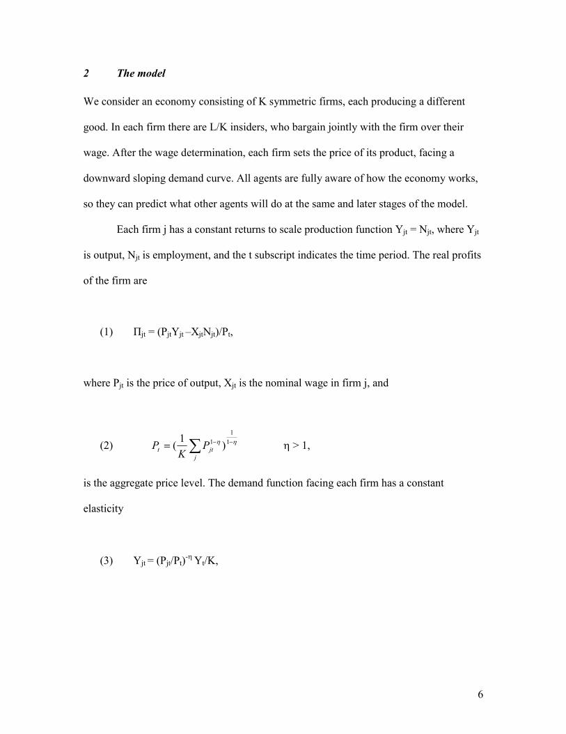
2 The model

We consider an economy consisting of K symmetric firms, each producing a different

good. In each firm there are L/K insiders, who bargain jointly with the firm over their

wage. After the wage determination, each firm sets the price of its product, facing a

downward sloping demand curve. All agents are fully aware of how the economy works,

so they can predict what other agents will do at the same and later stages of the model.

Each firm j has a constant returns to scale production function Yjt = Njt, where Yjt

is output, Njt is employment, and the t subscript indicates the time period. The real profits

of the firm are

(1) Πjt = (PjtYjt –XjtNjt)/Pt,

where Pjt is the price of output, Xjt is the nominal wage in firm j, and

(2) �� ��

��1

11 )1(

jjtt P

KP � > 1,

is the aggregate price level. The demand function facing each firm has a constant

elasticity

(3) Yjt = (Pjt/Pt)-� Yt/K,

6

where Yt is aggregate output.2

We now turn to the payoff function of the workers. Following Bhaskar (1990) we

assume that workers are concerned with fair treatment, and resent being treated worse

than identical workers elsewhere. Furthermore, their dissatisfaction from being paid less

than identical workers in other firms is greater than the benefit from being paid more.

Formally, the utility function of the workers is non-differentiable at the wage level of

other workers, so that the left-hand derivative is greater than the right-hand derivative.

There is considerable empirical support for an assumption of this kind. First, several

experimental studies report asymmetric effects of pay differences on levels of

satisfaction. Austin, McGinn and Susmilch (1980) employ a design in which subjects are

randomly divided into three groups. In one group, the subjects read a story in which they

are rewarded less pay than another identical worker; in the second, they receive equal

pay; in the third, they receive more pay. The subjects are then asked to rate their

satisfaction and fairness. The difference in satisfaction between the group paid more and

the group paid equally is much smaller than the difference in satisfaction between the

group paid equally and the group paid less. Ordonez, Connolly and Coughlan (2000)

have subjects read a story in which a focal MBA graduate and one or two other

comparison MBA graduates receive job offers. The number of comparison graduates and

the salaries all three receive are varied across the subjects. The reported decrease in

satisfaction when one of the comparison graduates has a higher offer is more than four

times higher than the reported increase in satisfaction when one of the comparison

graduates has a lower offer.

2 Equation (3) can be derived by assuming Dixit-Stiglitz preferences; see Blanchard and

7

Second, several studies report asymmetric aversion to inequity. Loewenstein,

Thompson and Bazerman (1989) report that subjects show strong aversion against

disadvantageous inequality; while many subjects also exhibit aversion to advantageous

inequality, this effect seems to be significantly weaker than the aversion to

disadvantageous inequality. Goeree and Holt (2000) document the existence of

asymmetric inequality aversion in experiments of alternating offers bargaining. Fehr and

Schmidt (1999) develop a theory of inequity aversion and show that it is able to explain a

number of seemingly puzzling findings in different economic situations.

Third, our assumption is also in accord with experiments on loss aversion, by

Kahneman and Tversky (1979) and others. These indicate that outcomes are not

perceived neutrally; rather, the value function appears to be steeper for losses than for

gains.

Finally, although for our results below we only require that workers have

asymmetries in preferences and not outcomes (e.g. effort), it is worth noting that Akerlof

(1984) reports that studies on the relationship between pay and effort generally find

stronger evidence for the withdrawal of services by workers who think they are

underpaid, than the positive effect on the effort of “overpaid” workers.3

Formally, we assume that the payoff function of a representative worker is

(4) ��

���

����

����

����

����

�

����

��

��

Gt

jtD

Jt

jt

t

jt

Gt

jt

Jt

jt

t

jtjt X

XXX

PX

XX

XX

PX

VVjt

,,

0 < �, � < 1, 0 < � + � < 1,

Kiyotaki (1985) for an early implementation in a macroeconomic model of price setting. 3 Danthine and Kurmann (2002) develop a sticky-wage model based on Akerlof’s related partial gift exchange idea.

8

where XJt is the average wage of workers in the same group, XGt is the average wage of

workers in the other group, and Djt is a dummy variable being one if Xjt < XJt and zero

otherwise. The payoff is continuous in real and relative wages, and strictly increasing in

the real wage. One would expect workers to prefer being paid more than others (�

positive); however, for the sake of generality we also allow for the possibility that

workers dislike inequality even if they gain themselves (� negative). In any case (4)

implies workers always prefer higher wages for given wages of others. The key

assumption is that the payoff is assumed to be non-differentiable at the point where

wages are equal to the wages of other workers in the same group, Xjt = XJt, so that the

loss in payoff of a reduction in the relative wage is strictly greater than the gain in payoff

of an increase in the relative wage. The non-differentiability only applies to workers in

the same group, which could reflect that workers in different groups are different, so that

the notion of equal wages for identical workers does not apply to workers in other groups.

Note, however, that allowing the comparison to workers in other groups to be non-

differentiable would strengthen our results. It would also be straightforward to generalize

the static results to n different groups.

With the exception of the non-differentiability assumption, the results are robust

to plausible variations in preferences. Working hours are treated as fixed, and are not

included. Employment is not included in (4), which could be justified by the assumption

that insiders are always employed, as variation in employment is undertaken by the firm

adjusting the hiring of new workers. However, the qualitative results would hold also if

workers were concerned about employment, or if working hours were allowed to vary.

9

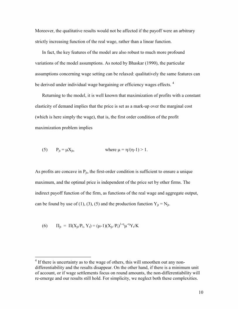
Moreover, the qualitative results would not be affected if the payoff were an arbitrary

strictly increasing function of the real wage, rather than a linear function.

In fact, the key features of the model are also robust to much more profound

variations of the model assumptions. As noted by Bhaskar (1990), the particular

assumptions concerning wage setting can be relaxed: qualitatively the same features can

be derived under individual wage bargaining or efficiency wages effects. 4

Returning to the model, it is well known that maximization of profits with a constant

elasticity of demand implies that the price is set as a mark-up over the marginal cost

(which is here simply the wage), that is, the first order condition of the profit

maximization problem implies

(5) Pjt = �Xjt, where � = �/(�-1) > 1.

As profits are concave in Pjt, the first-order condition is sufficient to ensure a unique

maximum, and the optimal price is independent of the price set by other firms. The

indirect payoff function of the firm, as functions of the real wage and aggregate output,

can be found by use of (1), (3), (5) and the production function Yjt = Njt.

(6) Πjt = Π(Xjt/Pt, Yt) = (�-1)(Xjt /Pt)1-��

-�Yt/K

4 If there is uncertainty as to the wage of others, this will smoothen out any non-differentiability and the results disappear. On the other hand, if there is a minimum unit of account, or if wage settlements focus on round amounts, the non-differentiability will re-emerge and our results still hold. For simplicity, we neglect both these complexities.

10

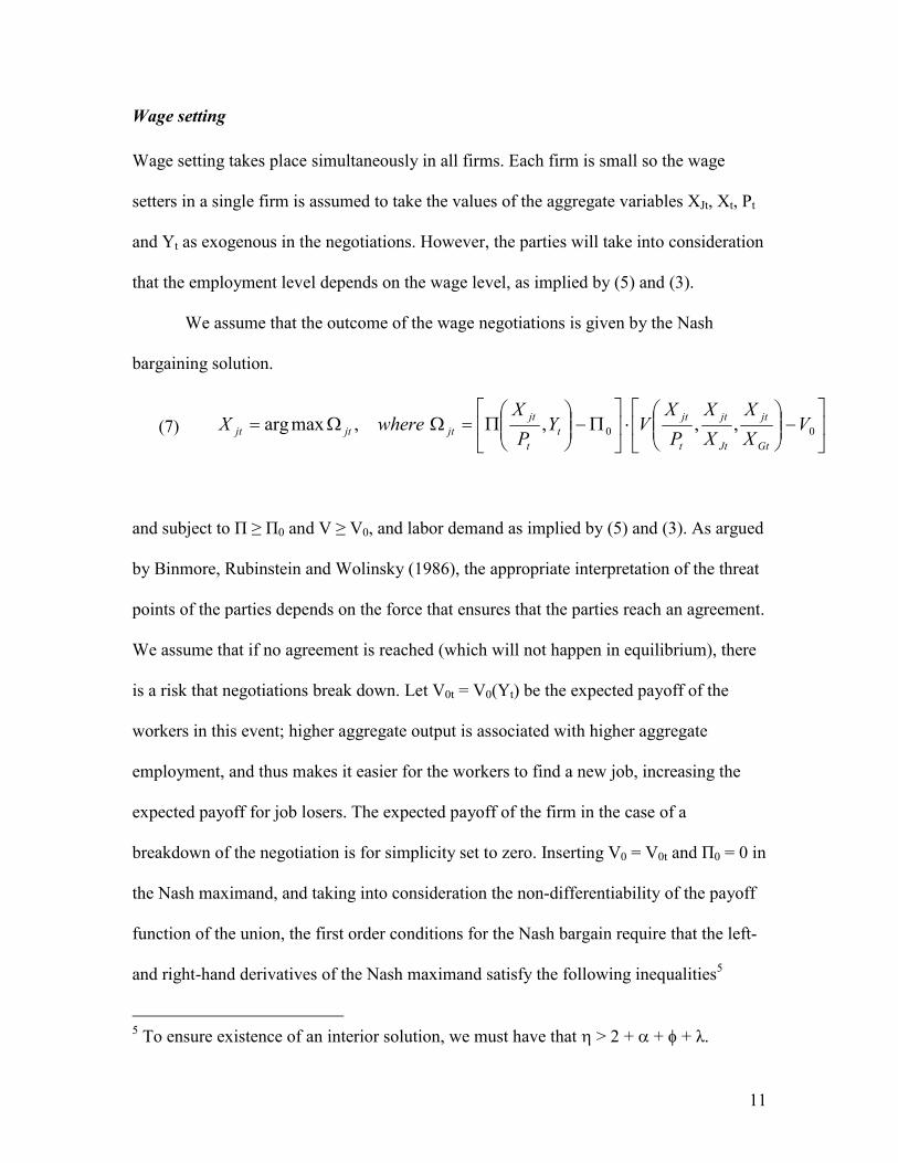
Wage setting

Wage setting takes place simultaneously in all firms. Each firm is small so the wage

setters in a single firm is assumed to take the values of the aggregate variables XJt, Xt, Pt

and Yt as exogenous in the negotiations. However, the parties will take into consideration

that the employment level depends on the wage level, as implied by (5) and (3).

We assume that the outcome of the wage negotiations is given by the Nash

bargaining solution.

(7) ��

���

����

���

��

�

���

�����

���

����� 00 ,,,,maxarg V

XX

XX

PX

VYP

XwhereX

Gt

jt

Jt

jt

t

jtt

t

jtjtjtjt

and subject to Π ≥ Π0 and V ≥ V0, and labor demand as implied by (5) and (3). As argued

by Binmore, Rubinstein and Wolinsky (1986), the appropriate interpretation of the threat

points of the parties depends on the force that ensures that the parties reach an agreement.

We assume that if no agreement is reached (which will not happen in equilibrium), there

is a risk that negotiations break down. Let V0t = V0(Yt) be the expected payoff of the

workers in this event; higher aggregate output is associated with higher aggregate

employment, and thus makes it easier for the workers to find a new job, increasing the

expected payoff for job losers. The expected payoff of the firm in the case of a

breakdown of the negotiation is for simplicity set to zero. Inserting V0 = V0t and Π0 = 0 in

the Nash maximand, and taking into consideration the non-differentiability of the payoff

function of the union, the first order conditions for the Nash bargain require that the left-

and right-hand derivatives of the Nash maximand satisfy the following inequalities5

5 To ensure existence of an interior solution, we must have that � > 2 + � + � + λ.

11

(8) � � 00 �����

��

��

jtjttjt

jt

jt

jt

jt

dXdVVV

dXd

dXd

(9) � � 00 �����

��

��

jtjttjt

jt

jt

jt

jt

dXdVVV

dXd

dXd .

In addition to (8) and (9), we know that either Xjt = XJt, or (8) or (9) hold with equality.

Let X-t = X-(XJt, XGt, Yt, Pt) and X+

t = X+( XJt, XGt,Yt, Pt) denote the wage levels

Xjt for which (8) and (9) respectively hold with equality. As shown in the appendix, we

know that X-( XJt, XGt, Yt, Pt) > X+( XJt, XGt, Yt, Pt). Furthermore, in the appendix we

also show the following result

Result 1: There exists a unique outcome Xjt to the wage bargaining in firm j, given by

(i) If XJt > X-t; Xjt = X-

t

(ii) If XJt � [X+t, X-

t] Xjt = XJt

(iii) If XJt < X+t; Xjt = X+

t

The intuition is in fact fairly simply. If the average wage in the group is within the range

[X+t, X-

t], the wage setting in firm j will match this wage. However, if the average wage

in the group is higher than the upper boundary X-t, workers in firm j are not able to match

this wage, but they are able to obtain a “high” wage X-t because of the high marginal

utility of wages when they have lower wages than the rest of the group. If the average

wage in the group is below the lower boundary X+t, workers in firm j will obtain more

12

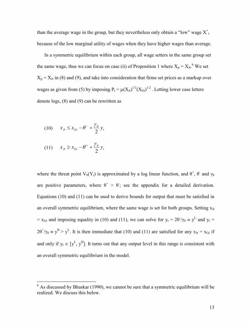
than the average wage in the group, but they nevertheless only obtain a “low” wage X+t

because of the low marginal utility of wages when they have higher wages than average.

In a symmetric equilibrium within each group, all wage setters in the same group set

the same wage, thus we can focus on case (ii) of Proposition 1 where Xjt = XJt.6 We set

Xjt = XJt in (8) and (9), and take into consideration that firms set prices as a markup over

wages as given from (5) by imposing Pt = �(XJt)1/2(XGt)1/2 . Letting lower case letters

denote logs, (8) and (9) can be rewritten as

(10) tGtJt yxx2

0�� ����

(11) tGtJt yxx2

0�� ����

where the threat point V0(Yt) is approximated by a log linear function, and θ+, θ- and γ0

are positive parameters, where θ+ > θ-; see the appendix for a detailed derivation.

Equations (10) and (11) can be used to derive bounds for output that must be satisfied in

an overall symmetric equilibrium, where the same wage is set for both groups. Setting xJt

= xGt and imposing equality in (10) and (11), we can solve for yt = 2θ-/γ0 � yL and yt =

2θ+/γ0 � yH > yL. It is then immediate that (10) and (11) are satisfied for any xJt = xGt if

and only if yt � [yL, yH]. It turns out that any output level in this range is consistent with

an overall symmetric equilibrium in the model.

6 As discussed by Bhaskar (1990), we cannot be sure that a symmetric equilibrium will be realized. We discuss this below.

13

The intuition for the range of equilibrium output levels is based on the feature that the

range of equilibrium wage levels in Result 1 is transformed into a range for output. As

long as output is within the range [yL, yH], workers in any individual firm are in a

position to obtain the same wage as workers in other firms; no more and no less. Output

above yH is not consistent with equilibrium, because then all workers would be in a

stronger position in the wage setting and they would all obtain higher wages than the

others, which is clearly impossible (formally, yt > yH would imply that xJt > xGt from (11),

thus violating the symmetric equilibrium condition xJt = xGt). Analogously, output below

yL would imply that all workers would get lower wages than the others, which is also

impossible.

Note that the existence of a range depends on the non-differentiability parameterized

by �. If �=0, so that the left- and right-hand derivatives (8) and (9) are equal, the range

for wages in Proposition 1 would collapse to a single point. Likewise, �=0 would imply

that θ- = θ+, implying that yL = yH so that output is uniquely determined.

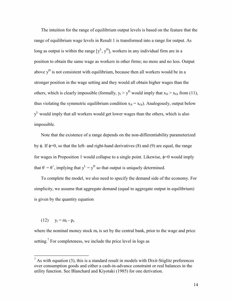
To complete the model, we also need to specify the demand side of the economy. For

simplicity, we assume that aggregate demand (equal to aggregate output in equilibrium)

is given by the quantity equation

(12) yt = mt - pt.

where the nominal money stock mt is set by the central bank, prior to the wage and price

setting.7 For completeness, we include the price level in logs as

7 As with equation (3), this is a standard result in models with Dixit-Stiglitz preferences over consumption goods and either a cash-in-advance constraint or real balances in the utility function. See Blanchard and Kiyotaki (1985) for one derivation.

14

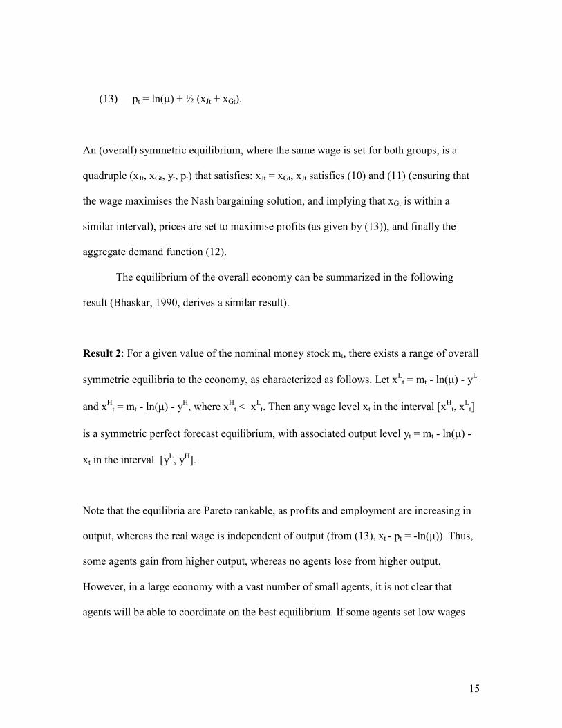
(13) pt = ln(�) + ½ (xJt + xGt).

An (overall) symmetric equilibrium, where the same wage is set for both groups, is a

quadruple (xJt, xGt, yt, pt) that satisfies: xJt = xGt, xJt satisfies (10) and (11) (ensuring that

the wage maximises the Nash bargaining solution, and implying that xGt is within a

similar interval), prices are set to maximise profits (as given by (13)), and finally the

aggregate demand function (12).

The equilibrium of the overall economy can be summarized in the following

result (Bhaskar, 1990, derives a similar result).

Result 2: For a given value of the nominal money stock mt, there exists a range of overall

symmetric equilibria to the economy, as characterized as follows. Let xLt = mt - ln(�) - yL

and xHt = mt - ln(�) - yH, where xH

t < xLt. Then any wage level xt in the interval [xH

t, xLt]

is a symmetric perfect forecast equilibrium, with associated output level yt = mt - ln(�) -

xt in the interval [yL, yH].

Note that the equilibria are Pareto rankable, as profits and employment are increasing in

output, whereas the real wage is independent of output (from (13), xt - pt = -ln(µ)). Thus,

some agents gain from higher output, whereas no agents lose from higher output.

However, in a large economy with a vast number of small agents, it is not clear that

agents will be able to coordinate on the best equilibrium. If some agents set low wages

15

xHt to ensure the Pareto optimal equilibrium with yH, they run the risk of getting lower

wages than others, with associated loss of utility.

An interesting possible solution to the coordination problem would apply if one

had a fully credible price or inflation target (see also McDonald and Sibly, 2001). If the

central bank could credibly announce a price target pE, ensuring that all agents indeed

expected pE to be realized, the Pareto optimal, high employment equilibrium could be

realized by setting m = yH - pE. However, in the sequel we will focus attention on a

situation without a credible price or inflation target.

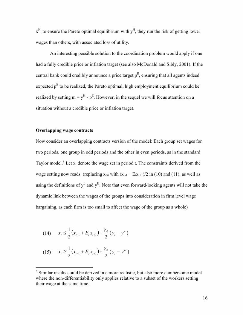
Overlapping wage contracts

Now consider an overlapping contracts version of the model: Each group set wages for

two periods, one group in odd periods and the other in even periods, as in the standard

Taylor model.8 Let xt denote the wage set in period t. The constraints derived from the

wage setting now reads (replacing xGt with (xt-1 + Etxt+1)/2 in (10) and (11), as well as

using the definitions of yL and yH. Note that even forward-looking agents will not take the

dynamic link between the wages of the groups into consideration in firm level wage

bargaining, as each firm is too small to affect the wage of the group as a whole)

(14) � � )(22

1 011

Lttttt yyxExx ����

��

�

(15) � � )(22

1 011

Httttt yyxExx ����

��

�

8 Similar results could be derived in a more realistic, but also more cumbersome model where the non-differentiability only applies relative to a subset of the workers setting their wage at the same time.

16

(14) and (15) can be rewritten as constraints on the nominal wage growth

(16) )(01L

tttt yyxEx ������

�

(17) )(01H

tttt yyxEx ������

�

Expectation formation

As before, the wage and price setting do not uniquely pin down the dynamics of output

and inflation. Although Equations (16) and (17) restrict wage growth to lie between

bounds, the multiplicity of equilibria implies that, otherwise, both output and inflation

depend on workers’ expectations. This implies that agents cannot deduce other agents’

behavior logically from the assumption that they behave rationally. In this situation it

seems reasonable to assume that agents base their beliefs regarding wage growth on the

past behavior of wage growth. This basic premise is common to a variety of approaches

to expectation formation. Evans and Honkapohja (2001) advocate adaptive learning as a

selection mechanism in situations with multiple rational expectations equilibria.

Experiments on games with a multiplicity of equilibria also show that agents learn from

the past behavior of other agents (Ochs, 1995). At the more general level, observing other

people’s behavior and making inferences on this basis is indeed how we form

expectations about other people’s behavior every day. If agents share this way of forming

expectations, it will work as a focal point or coordination mechanism for agents’

expectations.

17

Consider the following wage equation, representing a stylized version of existing

empirical wage equations

(18) �xt = β�xt-1 + (1-β)�xt-2 + 1(yt-1 – y*), 1 > 0.

(For convenience, we specify (18) to only include two lags, but will allow for more lags

in the empirical work.) Assuming that agents have observed wage inflation to adhere to

(18) in the past, it seems reasonable that they would expect wage inflation to follow (18)

in the future also, as long as this is consistent with the rational expectations equilibrium

of the model, ie. it satisfies the constraints given by (16) and (17). In other words, (18)

would work as a focal point for the wage setting behavior. Given that agents have these

beliefs, they would be self-fulfilling and thus both ex ante and ex post rational. In a

situation where agents set wages on the basis of (18), realization of another equilibrium

would require all agents to simultaneously switch to a different behavior. If one

disregards such simultaneous switches, the unique equilibrium outcome in this situation

would be that agents continue to set wages according to (18).

Note also that if a share, however small, of the agents in the economy has

adaptive expectations according to (18), this will serve as a coordination mechanism so

that (18) is the unique strategy consistent with rational expectations (as also observed by

Bhaskar, 1990).

Given (18), y* is the unique long run equilibrium rate of output. Output cannot

remain above or below y*, as this would lead to consistently increasing or decreasing

nominal wage growth. Note however that y* is inherently expectations based. y* should

not be interpreted as the natural rate as given by other considerations like search behavior

18

or efficiency wages; the equivalent to these considerations are already captured in the

model described in Result 2, which had a range of equilibria. If agents’ expectations

change, for instance they believe that the labor market has changed so that stable nominal

wage growth is consistent with higher output y** rather than y*, this would imply a

change in the long run equilibrium to the new level y**, as long as y** is within [yL, yH].

The important role of expectations in determining y* suggests that one cannot

expect to find a stable relationship between output and inflation. And this is indeed the

case: Staiger, Stock and Watson (1997) find considerable imprecision in the estimates of

the natural rate, and there has been considerable debate over the last decade in the U.S.

over whether the decline in unemployment without a corresponding rise in inflation is

evidence of a decrease in the natural rate. This noisy behavior is, however, consistent

with our story. The structure of the labor market, and of price and wage setting, do not

pin down a tight relationship between inflation and unemployment. In our model,

expectations play a large role, and one is less surprised to find more noise and

fluctuations, because expectations are likely to be more volatile than other features like

preferences and technology.

The implications of the adaptive expectations focal point relationship (18) are

well-known; the key novelties in this paper are the implications of the constraints (16)

and (17). It turns out the existence of these constraints makes the model highly complex

when agents are forward-looking. To evaluate whether the constraints bind, agents need

to not only know the current money stock, but also to form expectations of the entire

future path of monetary policy.

19

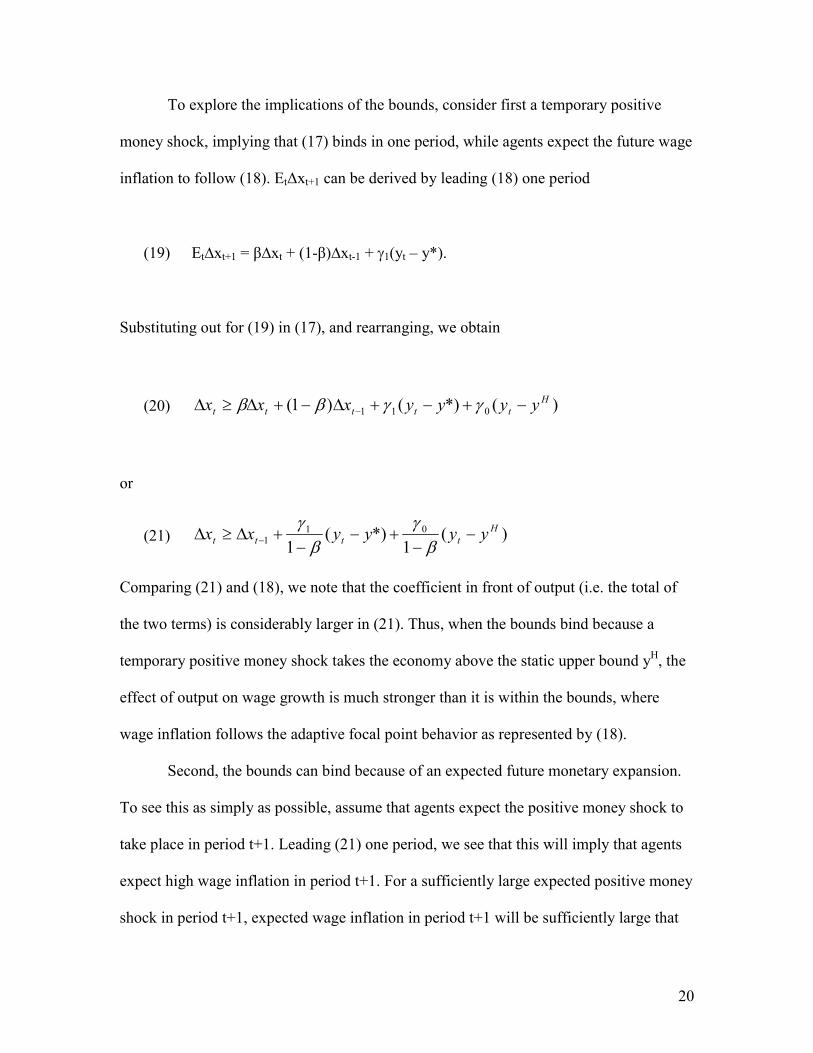
To explore the implications of the bounds, consider first a temporary positive

money shock, implying that (17) binds in one period, while agents expect the future wage

inflation to follow (18). Et∆xt+1 can be derived by leading (18) one period

(19) Et�xt+1 = β�xt + (1-β)�xt-1 + 1(yt – y*).

Substituting out for (19) in (17), and rearranging, we obtain

(20) )(*)()1( 011H

ttttt yyyyxxx �����������

����

or

(21) )(1

*)(1

011

Htttt yyyyxx �

���

�����

�

�

�

�

�

Comparing (21) and (18), we note that the coefficient in front of output (i.e. the total of

the two terms) is considerably larger in (21). Thus, when the bounds bind because a

temporary positive money shock takes the economy above the static upper bound yH, the

effect of output on wage growth is much stronger than it is within the bounds, where

wage inflation follows the adaptive focal point behavior as represented by (18).

Second, the bounds can bind because of an expected future monetary expansion.

To see this as simply as possible, assume that agents expect the positive money shock to

take place in period t+1. Leading (21) one period, we see that this will imply that agents

expect high wage inflation in period t+1. For a sufficiently large expected positive money

shock in period t+1, expected wage inflation in period t+1 will be sufficiently large that

20

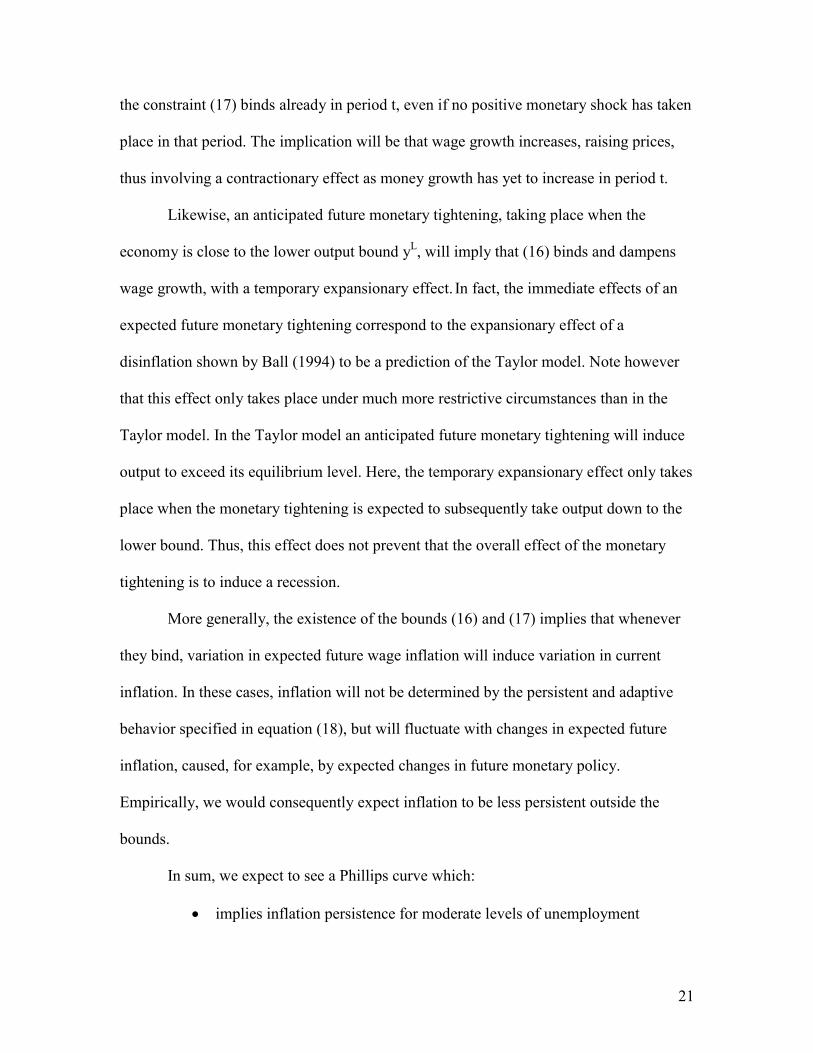
the constraint (17) binds already in period t, even if no positive monetary shock has taken

place in that period. The implication will be that wage growth increases, raising prices,

thus involving a contractionary effect as money growth has yet to increase in period t.

Likewise, an anticipated future monetary tightening, taking place when the

economy is close to the lower output bound yL, will imply that (16) binds and dampens

wage growth, with a temporary expansionary effect. In fact, the immediate effects of an

expected future monetary tightening correspond to the expansionary effect of a

disinflation shown by Ball (1994) to be a prediction of the Taylor model. Note however

that this effect only takes place under much more restrictive circumstances than in the

Taylor model. In the Taylor model an anticipated future monetary tightening will induce

output to exceed its equilibrium level. Here, the temporary expansionary effect only takes

place when the monetary tightening is expected to subsequently take output down to the

lower bound. Thus, this effect does not prevent that the overall effect of the monetary

tightening is to induce a recession.

More generally, the existence of the bounds (16) and (17) implies that whenever

they bind, variation in expected future wage inflation will induce variation in current

inflation. In these cases, inflation will not be determined by the persistent and adaptive

behavior specified in equation (18), but will fluctuate with changes in expected future

inflation, caused, for example, by expected changes in future monetary policy.

Empirically, we would consequently expect inflation to be less persistent outside the

bounds.

In sum, we expect to see a Phillips curve which:

� implies inflation persistence for moderate levels of unemployment

21

� implies stronger effects of monetary policy at low or high levels of

unemployment than for intermediate levels of unemployment

� implies less inflation persistence and has a different slope for low and high

levels of unemployment

3 Empirical Specification

To test the predictions, we adopt a levels version of Staiger, Stock and Watson (1997)’s

specification:

(22) �t = �0 +�1�t-1 +�2�t-2 +�3�t-3 + 1ut-1 + 2ut-2 + Zt

+�H0IH +�H

1 IH � t-1 +�H2 IH �t-2 +�H

3 IH �t-3

+ H1 IH (ut-1 -uH )+ H

2 IH (ut-2 -uH )+ H IH Zt

+�L0IL +�L

1 IL � t-1 +�L2 IL �t-2 +�L

3 IL �t-3

+ L1 IL (ut-1 - uL)+ L

2 IL (ut-2 - uL )+ L ILZt +�t ,

where �t ≡ pt-pt-1, IH is a dummy variable taking the value 1 when u> uH, IL is a dummy

variable taking the value 1 when u< uL, and Z represents a vector of proxies for aggregate

supply shocks. Following common practice we have invoked an Okun’s Law relationship

to replace output with unemployment. This has the advantage that it is not necessary to

make assumptions concerning the stationarity of output. The interaction of the dummy

variables with the inflation and unemployment terms above and below the bounds allows

us to test the model’s prediction that the short-run dynamics of inflation and

unemployment differ for low and high levels of unemployment.

22

Aside from the inclusion of interaction terms to allow inflation dynamics to

change outside the bounds, we depart from Staiger, Stock and Watson (1997) in two

ways. First, as noted above, we write the equation in levels; this allows us to more easily

compare our results with previous estimates of the Phillips curve and evaluate the

behavior of inflation persistence. Second, we do not explicitly attempt to estimate a time-

varying natural rate of unemployment.9 While there in general is reason to believe that

parameters change over time, allowing for a time-varying natural rate in addition to the

bounds would presumably be to ask for too much from the data.

We include supply shock variables for two related reasons. First, they represent

deviations from the inflationary dynamics implied by the other coefficients in the model,

and thus need to be controlled for to prevent omitted variable bias. Second, in principle

equation (22) represents only one equation in a two-equation system (the other equation

being the aggregate demand curve with unemployment substituted for output). OLS

estimates of (22) will therefore suffer from simultaneous equations bias. The bias in

estimating the aggregate supply coefficients will depend on the relative variance of the

aggregate supply shocks to the aggregate demand shocks. By trying to proxy for the

largest aggregate supply shocks, we reduce the variance of the unexplained portion of the

aggregate supply shocks, and thus reduce the amount of the bias.10

The bounds, uH and uL as derived from yH and yL, are determined by structural

parameters of the model, including how the threat point depends on output and the size of

9 Although the presence of the interaction terms between the dummy variables and constants does implicitly allow for this possibility during time of high and low unemployment. 10 An alternative but complementary approach would be to estimate (22) via instrumental variables using an instrument for exogenous variations in aggregate demand or supply.

23

the kink in preferences. Although in principle one could calibrate the size of the bounds,

or, more simply, the size of yH – yL by picking values for the parameters, it is not clear

what reasonable values for some of the parameters are. Were the bounds known, (22)

would be estimable via OLS. Although they are not known, it is possible to estimate them

endogenously. We follow the structural break literature11 by reestimating (25) for

different values of uH and uL and picking the specification yielding the highest value for

the log-likelihood.

4 Data and Estimation Results

We use the unemployment rate for all civilians age 16 and over, seasonally adjusted,

monthly, and the CPI for all urban consumers, seasonally adjusted, monthly.12 We

average the data to obtain quarterly figures, and construct an inflation measure by

multiplying the percent change in the CPI by 400.

Following Ball and Mankiw (1995),13 we use three supply shock measures:

11 See Quandt (1958) and Maddala and Kim (1998) 12 We have also tried the demography-adjusted unemployment rates created by Shimer (1998), which captures the idea that the natural rate of unemployment may change over time due to changes in demographic variables (since the young are more likely to be unemployed than the old). The coefficient estimates were generally little changed, and the fit in terms of adjusted R squared worse, so we stick to the model with the ordinary unemployment series. 13 We choose these measures of food and energy aggregate supply shocks rather than the alternative, also PPI-based, measures used in Staiger, Stock and Watson (1997) because the energy price measure used there has become significantly more volatile and highly negatively autocorrelated since 1995, suggesting a change in definition of the series.

24

1. FOOD, constructed by taking the difference in inflation rates between the

processed foods and feeds component of the PPI (series 1300) and PPI

inflation

2. FUEL, constructed by taking the difference in inflation rates between the fuel

and energy component of the PPI (series 1100) and PPI inflation

3. NIXON, a dummy for the wage and price controls in the Nixon and Ford

administrations introduced by Gordon (1990).

We begin the sample in 1955:I, avoiding the effects of wage and price controls imposed

during the Korean War, and we end it in 2000:IV.

Table 1 provides the main empirical results. The first column of Table 1 reports

the results of estimating (22) without any bounds. The coefficients on unemployment

alternate in sign but do sum to -.213, so that the Phillips curve is downward sloping, as

one would hope. Also as expected, the coefficients on lagged inflation are all positive and

sum to 1.004, implying inflation is persistent.

The next three columns report the results of imposing the bounds, endogenously

determined by the method described above. The first column reports the coefficients on

output, inflation and the supply shocks between the bounds, the next columns the

additional effects below and above the bounds. We find the bounds to be at 4.7 and 6.5

percent, which correspond to (approximately) the 30th and 70th percentiles of observed

unemployment.14 Note that the more elaborate specification allowing all coefficients to

14 Since our technique may also pick up any possible non-linearity in the Phillips curve, we restrict the bounds to lie above and below the median value of unemployment observed. If we relax this restriction, the estimated bounds lie at 9.9 and 10.1 percent, the third-highest and second-highest unemployment rates observed.

25

take different values outside the bounds, as predicted by our model, is supported by the

data, as the restrictions that are involved by the regression without bounds (column 1) is

rejected in a likelihood ratio test at the one percent level.

The third and fourth columns report the interaction terms describing how the

coefficients change outside the bounds. First, note that the coefficients on the lagged

inflation interaction terms are almost all negative- implying that inflation is less persistent

both below and above the bounds, as predicted by our model. Below the bounds, the

interaction terms sum to -.775 and above to -.453, which are large in magnitude and

statistically significant.

Below the bounds, the interaction terms on unemployment sum to –1.378,

implying that the Phillips curve is more steeply sloped, as predicted by our model. Above

the bounds, however, the unemployment terms sum to .587, which is close in magnitude

to the value of .608 estimated between the bounds, implying a nearly-flat Phillips curve

above the bound (although highly imprecisely determined), in contrast to the predictions

of our model.

Table 2 evaluates the prediction that the effect of contractionary and expansionary

monetary policy disturbances are different outside and between the bounds; one set shifts

the Phillips curve, the other represents shifts along the Phillips curve. We use the measure

of monetary policy derived by Bernanke and Mihov (1998) from a structural VAR model

of the Federal Funds market. This measure essentially purges endogenous policy

movements from the Federal Funds rate. From that variable, we construct a series

consisting only of contractionary changes in policy and a series consisting only of

expansionary changes. The variable is defined only over the period from 1966 to 1996,

26

where the starting date is determined by the change of the Federal Reserve’s policy

instrument to the Federal Funds rate. For dates outside those years, we set the value for

the contractionary and expansionary variables to zero.

The first column reports results not imposing any bounds; monetary expansions

have a small and statistically insignificant effect, while monetary contractions have a

larger and statistically significant negative effect.

The remaining two columns report the results imposing the bounds. The bounds

are estimated to be at unemployment rates of 4.7 and 6.5, unchanged from Table 1; the

coefficients on lagged inflation and unemployment are also not much changed. The

results are largely consistent with our model: monetary policy expansions have a more

positive effect outside the bounds (although significant only for high unemployment),

while monetary contractions have a significant negative effect for high unemployment.

5 Conclusion

Standard rational-expectations formulations of the aggregate supply curve, such as those

of Fischer (1978), Taylor (1980) and Calvo (1983) are unable to replicate the persistence

of inflation observed in the data. We suggest that coordination problems and multiple

equilibria are the keys to explaining inflation persistence. When there is a range of

possible equilibria, there is scope for past behavior to play a role as an equilibrium

selection device. Several possible mechanisms can generate a range of equilibria; we

focus on a wage-contracting model in which (following Bhaskar, 1990) workers care

disproportionately more about being paid less than other workers than they do about

being paid more than other workers. We argue that as wage setters want to match the

27

wage growth set by others, the behavior of wages in the recent past will be a natural

starting point for expectations. Within the range of equilibria, such beliefs will create a

self-fulfilling prophecy; and thus be consistent with rational expectations. These beliefs

will combine the attractive features of both adaptive and rational expectations; they will

be consistent with key features on actual inflation series, while at the same time not being

based on agents making systematic errors.

Replacing output with unemployment, we estimate the model, including the

bounds, on quarterly data over the period 1955-2000. We find that the dynamics of the

Phillips curve do change at unemployment rates below 4.7 percent and above 6.5 percent.

As predicted by our model, inflation seems less persistent outside the bounds. The

prediction that inflation is more sensitive to changes in unemployment outside the bounds

receives mixed results: we find stronger effects for low unemployment, but not for high

unemployment. We also find that monetary policy contractions and expansions shift the

position of the Phillips curve outside the bounds, as predicted by our model (but only

significant for monetary contractions for high levels of unemployment).

At the more general level our story is easier to reconcile with the rather erratic

relationship between inflation and unemployment that exists in the data than more

traditional models. In such models, the erratic behavior is often explained as arising from

a time-varying NAIRU. However, a problem with this explanation is that attempts to

identify the structural determinants of the NAIRU are generally disappointing (see, for

example, Staiger, Stock and Watson, 2001). In our model, expectations play a large role,

and one is less surprised to find more noise and fluctuations, as expectations may well be

more volatile than other features like preferences and technology.

28

We view our evidence as supportive of the existence of a range of equilibria for

unemployment, and inflation being less persistent outside this range. However, as our

evidence is based on inflation and unemployment, it can clearly not discriminate between

our story of fair treatment, and possible other stories also generating the same

macroeconomic characteristics.

In our model, inflation persistence is generated as a focal point for agents’

expectations, and it is not an inherent feature derived from preferences and technology.

This implies that inflation persistence may weaken or disappear if another focal point

becomes more prominent. Indeed, Ball (2000) showed that in the period from 1879

through 1914, when the US had a gold standard, the price level was close to a random

walk, implying that inflation is white noise. During this period, an even simpler

expectation formation than the one presented here may be the most appropriate, namely

that expected inflation was close to a constant (Ball, 2000).

In recent years, a possible candidate for a focal point for inflation expectations

would be the inflation target of the central bank. If agents believe that the central bank

will fulfill its inflation target, this can work as a coordinating device for expectations, as

long as output remains without the equilibrium range. Somewhat speculatively, this

suggests the following interpretation of why the high growth and falling unemployment

in the US in the late 1990s did not lead to increasing inflation: the Federal Reserve

commanded high credibility so that private agents expected the low inflation to continue,

and thus set wages and prices according to this premise.

The use of preferences exhibiting loss aversion or other departures from standard

assumptions has become commonplace in the study of consumption and asset pricing,

29

and has been used to attempt to explain various empirical puzzles in those literatures. In

this paper, we take a step towards applying preferences taken from behavioral economics

to explain the empirical puzzle in the Phillips curve literature of inflation persistence. We

show that a relatively minor departure from standard assumptions not only yields

inflation persistence, but also sheds light on why the relationship between output and

inflation is noisy and erratic.

30

References

Akerlof, George (1984). “Gift Exchange and Efficiency Wage Theory: Four Views.” American Economic Review Papers and Proceedings, 74, pp 79-83. Austin, William, Neil C. McGinn and Charles Susmilch (1980). “Internal Standards Revisited: Effects of Social Comparisons and Expectancies on Judgments of Fairness and Satisfaction.” Journal of Experimental Social Psychology, 16, pp. 426-441. Ball, Laurence S. (2000). “Near-Rationality and Inflation in Two Monetary Regimes.” NBER Working Paper 7988. ----------- and Mankiw, N. Gregory (1995). “Relative-Price Changes as Aggregate Supply Shocks.” Quarterly Journal of Economics, CV:2, pp. 161-193. Bernanke, Ben S. and Ilian Mihov (1998). “Measuring Monetary Policy.” Quarterly Journal of Economics, CVIII:3, pp. 869-902. Bhaskar, V. (1990). “Wage relatives and the natural range of unemployment.” Economic Journal 100, 60-66.

Blanchard, Olivier J. and Nobuhiro Kiyotaki (1985). “Monopolistic competition and the effects of aggregate demand.” American Economic Review, pp. 647-667. Binmore, Ken., Ariel Rubinstein, and Asher Wolinsky (1986).”The Nash bargaining solution in economic modelling.” RAND Journal of Economics,17, pp176-188. Bårdsen, G., E. Jansen and R. Nymoen (2002). ”Testing the New-Keynesian Phillips Curve”, Mimeo, University of Oslo. Calvo, Guillermo (1983). “Staggered Prices in a Utility-Maximizing Framework.” Journal of Monetary Economics 12:4, pp. 983-998. Cooper, Russell W. (1999). Coordination Games: Complementarities and Macroeconomics. Cambridge University Press. Danthine, Jean-Pierre and Andre Kurmann. “Fair Wages in a New Keynesian Model of the Business Cycle.” Mimeo, University of Virginia. Evans, George W. and Seppo Honkaphohja (2001). Learning and Expectations in Macroeconomics. Princeton: Princeton University Press. Fehr, E. and K. M. Schmidt. (1999).A Theory of Fairness, Competition, and Cooperation. Quarterly Journal of Economics CXIV, pp. 769-816.

31

Fischer, Stanley. (1977). “Long-Term Contracts, Rational Expectations, and the Optimal Money Supply Rule.” Journal of Political Economy 85:2, pp. 191-205. Friedman, Milton (1968). “The Role of Monetary Policy.” American Economic Review, 58:1, pp. 1-17. Fuhrer, Jeffrey and Gerald Moore (1995). “Inflation persistence.” Quarterly Journal of Economics ,CX, pp. 127-160. Gali, Jordi and Mark Gertler (1999). “Inflation Dynamics: A Structural Econometric Analysis.” Journal of Monetary Economics 44, 195-222. Goeree, J.K and C. A Holt. “Asymmetric Inequality Aversion and Noisy Behavior in Alternating-Offer Bargaining." European Economic Review 44, pp. 1079-1089. Gordon, Robert J. (1990). “What is New-Keynesian Economics?” Journal of Economic Literature, XXVIII:3, pp. 1115-1171. Kahneman, Daniel and Amos Tversky (1979). “Prospect Theory: An Analysis of Decision under Risk.” Econometrica, 47, pp 263-291. Loewenstein, George F., Leigh Thompson, and Max H. Bazerman. (1989). Social Utility and Decision Making in Intermpersonal Contexts. “ Journal of Personality and Social Psychology LVII, pp 426-441. Lye, I, I. M. McDonald and H. Sibly (2001). “An Estimate of the Range of Equilibrium Rates of Unemployment for Australia.” Economic-Record 77, 35-50. Maddala, G. S. and In-Moo Kim (1998). Unit Roots, Cointegration and Structural Change. Cambridge University Press, Cambridge UK. Mankiw, N. Gregory (2001). “The Inexorable and Mysterious Tradeoff Between Inflation and Unemployment.” Economic Journal 111. C45-61. McDonald, Ian (1995). “Models of the range of equilibria.” In Rod Cross (ed). The Natural Rate of Unemployment: Reflections on 25 years of the hypothesis. Cambridge: Cambridge University Press. McDonald, Ian (2001). “Reference Pricing, Inflation Targeting and the Non-inflationary Expansion.” Mimeo, University of Melbourne. Ochs, Jack (1995). “Coordination Problems”. In John H. Kagen and Alvin Roth (eds). Handbook of Experimental Economics. Princeton: Princeton University Press.

32

Ordonez, Lisa D., Terry Connolly and Richard Coughlan (2000). “Multiple Reference Points in Satisfaction and Fairness Assessment.” Journal of Behavioral Decision Making, 13, pp. 329-244. Phillips, A. W. (1959). “The Relation Between Unemployment and the Rate of Change of Money Wages in the United Kingdom 1861-1957.” Economica, 25:2, pp. 283-299. Quandt, Richard E. (1958). “The Estimation of the Parameters of a Linear Regression System Obeying Two Separate Regimes.” Journal of the American Statistical Association, pp. 873-880. Roberts, John. (1998). Inflation expectations and the transmission of monetary policy. Board of Governors of the Federal Reserve System. Sbordone, Argia M. (2002). “Prices and Unit Labor Costs: A New Test of Price Stickiness.” Journal of Monetary Economics, 49(2), pp. 265-292. Shimer, Robert (1998). “Why is the U.S. Unemployment Rate So Much Lower?” NBER Macroeconomics Annual, pp. 11-61. Sims, Christopher A. (1992). “Interpreting the Macroeconomic Time Series Facts: The Effects of Monetary Policy.” European Economic Review, 36(4), pp. 975-1011. Staiger, Douglas, James Stock and Mark Watson (1997). “How Precise Are Estimates of the Natural Rate of Unemployment?” In Christina D. Romer and David H. Romer (eds). Reducing Inflation: Motivation and Strategy, Chicago University Press. ---------------- (2001). “Prices, Wages and the U.S. NAIRU in the 1990s”. Mimeo, Kennedy School of Government, Harvard University. Taylor, John. (1980). “Aggregate dynamics and staggered contracts.” Journal of Political Economy LXXXVIII, 1-24. --------------- (1999). “Staggered wage and price setting in macroeconomics.” Chapter 15 in J. B. Taylor and M. Woodford (eds). Handbook of Macroeconomics. North-Holland. Woglom, Geoffrey (1982). “Underemployment Equilibrium with Rational Expectations.” Quarterly Journal of Economics 9, 89-107.

33

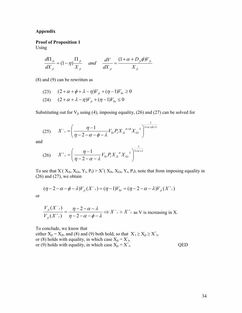
Appendix Proof of Proposition 1 Using

jt

jtjt

jtjt

jt

jt

jt

XVD

dXdVand

XdXd )1(

)1(��

���

��

���

(8) and (9) can be rewritten as

(23) 0)1()2( 0 ������� tjt VV �����

(24) 0)1()2( 0 ������ tjt VV ����

Substituting out for Vjt using (4), imposing equality, (26) and (27) can be solved for

(25) ���

���

����

� �����

���

����

�

����

��

11

021

GtJtttt XXPVX

and

(26) ��

��

���

� ��

�

���

����

�

���

��

11

021

GtJtttt XXPVX

To see that X-( XJt, XGt, Yt, Pt) > X+( XJt, XGt, Yt, Pt), note that from imposing equality in (26) and (27), we obtain

)()2()1()()2( 0 tjtttjt XVVXV ��

���������� �������� or

tttjt

tjt XXXVXV

��

�

�

��

����

����

����

���

22

)()(

as V is increasing in X.

To conclude, we know that either Xjt = XJt, and (8) and (9) both hold, so that X-

t ≥ Xjt ≥ X+t,

or (8) holds with equality, in which case Xjt = X-t,

or (9) holds with equality, in which case Xjt = X+t. QED

34

Derivation of (10) and (11) Using the same procedure as in the proof of Proposition 1, (8) and (9) can be rearranged to

(27) ���

���

����

� ����

���

����

�

����

��

11

021

GtJtttjt XXPVX

and

(28) ��

��

���

� ��

���

����

�

���

��

11

021

GtJtttjt XXPVX

Imposing Xjt = XJt and Pt = µ(XJt)1/2(XGt)1/2, and rearranging, we obtain

(29) �

����

���

���

����

�

����

�� 2/1

1

0 )(2

)1(tGtJt YVXX .

(30) �

���

���

���

����

�

���

�� 2/1

1

0 )(2

)1(tGtJt YVXX .

Using the log linear approximations

(31) 1

0 1/ 20

( 1)ln ( )2 2t ty V Y �� � �

�� � � �

� �� ��

� � � � �� � � ��

.

(32) 1

0 1/ 20

( 1)ln ( )2 2t ty V Y �� � �

�� � �

� �� ��

� � � � �� � ��

.

we obtain (10) and (11) in the main text

35

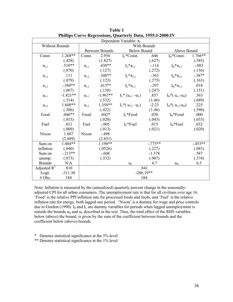
Table 1 Phillips Curve Regressions, Quarterly Data, 1955:I-2000:IV

Dependent Variable: �t Without Bounds With Bounds

Between Bounds Below Bound Above Bound Const.

1.268** (.428)

Const.

2.956 (1.827)

IL*Const.

.646 (.627)

IH*Const.

1.766** (.585)

�t-1

.510** (.070)

�t-1

.438** (.127)

IL*�t-1

-.114 (.272)

IH*�t-1

-.083 (.156)

�t-2

.111 (.079)

�t-2

.348** (.123)

IL*�t-2

-.363 (.275)

IH*�t-2

-.387* (.163)

�t-3

-.384** (.067)

�t-3

.413** (.130)

IL*�t-3

-.297 (.247)

IH*�t-3

.018 (.151)

ut-1

-1.821** (.314)

ut-1

-1.967** (.532)

IL* (ut-1 –uL)

.857 (1.46)

IH*( ut-1-uH)

.363 (.689)

ut-2

1.608** (.306)

ut-2

1.358** (.422)

IL*( ut-2 –uL)

-2.23 (1.46)

IH*( ut-2-uH)

.225 (.590)

Food

.046** (.015)

Food

.042* (.020)

IL*Food

.030 (.043)

IH*Food

.000 (.033)

Fuel

.011 (.009)

Fuel

-.005 (.013)

IL*Fuel

.015 (.021)

IH*Fuel

.032 (.020)

Nixon

1.807 (2.889)

Nixon

-.498 (2.851)

Sum on inflation

1.004** (.040) 1.198**

(.0526) -.775** (.227) -.453**

(.083) Sum on unemp.

-.213** (.073) -.608

(.332) -1.378 (.907) .587

(.374) Bounds N/A uL 4.7 uH 6.5

Adjusted R2 .810 LogL -311.30 # Obs. 184

.841 -286.19**

184 Note: Inflation is measured by the (annualized) quarterly percent change in the seasonally-adjusted CPI for all urban consumers. The unemployment rate is that for all civilians over age 16. ‘Food’ is the relative PPI inflation rate for processed foods and feeds, and ‘Fuel’ is the relative inflation rate for energy, both lagged one period. ‘Nixon’ is a dummy for wage and price controls due to Gordon (1990). IH and IL are dummy variables for periods when lagged unemployment is outside the bounds uH and uL described in the text. Thus, the total effect of the RHS variables below (above) the bound, is given by the sum of the coefficient between bounds and the coefficient below (above) bounds. * Denotes statistical significance at the 5% level ** Denotes statistical significance at the 1% level

36

37

Table 2 Phillips Curve Regressions, 1955:I-2000:IV

With Monetary Policy Indicator Dependent Variable: �t

Without Bounds With Bounds Between Bounds Below Bound Above Bound

Const.

1.125* (.498)

Const.

1.690 (1.868)

IL*Const.

.785 (.685)

IH*Const.

1.190 (.645)

�t-1

.442** (.068)

�t-1

.341* (.131)

IL*�t-1

-.011 (.274)

IH*�t-1

.020 (.160)

�t-2

.048 (.077)

�t-2

.352** (.125)

IL*�t-2

-.351 (.275)

IH*�t-2

-.446** (.165)

�t-3

.388** (.063)

�t-3

.459** (.128)

IL*�t-3

-.359 (.242)

IH*�t-3

-.061 (.150)

ut-1

-1.531** (.324)

ut-1

-1.479** (.573)

IL* (ut-1 –uL)

.544 (1.525)

IH*( ut-1-uH)

.118 (.731)

ut-2

1.354** (.299)

ut-2

1.127** (.431)

IL*( ut-1 –uL)

-1.817 (1.502)

IH*( ut-2-uH)

.111 (.596)

Food

.036* (.015)

Food

.043* (.019)

IL*Food

.024 (.044)

IH*Food

-.004 (.033)

Fuel

.001 (.001)

Fuel

.001 (.013)

IL*Fuel

.012 (.021)

IH*Fuel

.027 (.020)

Nixon

.181 (2.776)

Nixon

-.010 (3.068) N/A N/A

Monetary Expansion

.0774 (.060)

Monetary Expansion

-.205 (.127) .556

(.712) .335* (.154)

Monetary Contraction

-.254** (.057)

Monetary Contraction

-.063 (.077) -.017

(.197) -.595** (.222)

Sum on inflation

.877** (.049) 1.152**

(.072) -.721** (.252) -.487**

(.103) Sum on unemp.

-.176 (.097) -.351

(.343) -1.273 (1.085) .228

(.403) Bounds N/A uL 4.7 uH 6.5

Adjusted R2 .828

LogL -301.32 # Obs. 184

.851 -276.91**

184

Note: ‘Monetary Contractions’ represents the value of the Bernanke and Mihov (1998) indicator for monetary policy when that indicator is negative, and ‘Monetary Expansions’ the value of that indicator when the indicator is positive. All other notation as in Table 1. * Denotes statistical significance at the 5% level ** Denotes statistical significance at the 1% level