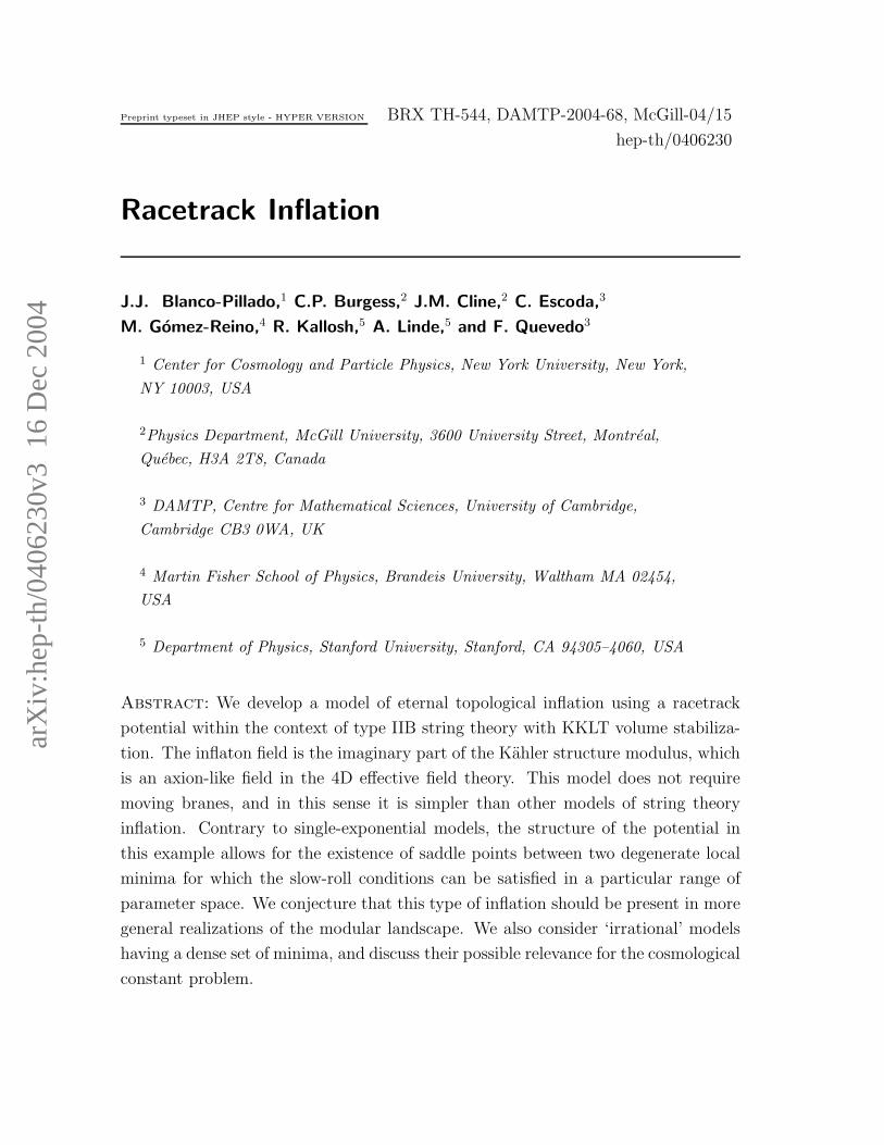
arX

iv:h

ep-t

h/04

0623

0v3

16

Dec

200

4

Preprint typeset in JHEP style - HYPER VERSION BRX TH-544, DAMTP-2004-68, McGill-04/15

hep-th/0406230

Racetrack Inflation

J.J. Blanco-Pillado,1 C.P. Burgess,2 J.M. Cline,2 C. Escoda,3

M. Gomez-Reino,4 R. Kallosh,5 A. Linde,5 and F. Quevedo3

1 Center for Cosmology and Particle Physics, New York University, New York,

NY 10003, USA

2Physics Department, McGill University, 3600 University Street, Montreal,

Quebec, H3A 2T8, Canada

3 DAMTP, Centre for Mathematical Sciences, University of Cambridge,

Cambridge CB3 0WA, UK

4 Martin Fisher School of Physics, Brandeis University, Waltham MA 02454,

USA

5 Department of Physics, Stanford University, Stanford, CA 94305–4060, USA

Abstract: We develop a model of eternal topological inflation using a racetrack

potential within the context of type IIB string theory with KKLT volume stabiliza-

tion. The inflaton field is the imaginary part of the Kahler structure modulus, which

is an axion-like field in the 4D effective field theory. This model does not require

moving branes, and in this sense it is simpler than other models of string theory

inflation. Contrary to single-exponential models, the structure of the potential in

this example allows for the existence of saddle points between two degenerate local

minima for which the slow-roll conditions can be satisfied in a particular range of

parameter space. We conjecture that this type of inflation should be present in more

general realizations of the modular landscape. We also consider ‘irrational’ models

having a dense set of minima, and discuss their possible relevance for the cosmological

constant problem.

Contents

1. Introduction 1

2. Eternal Topological Inflation 3

3. Racetrack Inflation 5

3.1 The Effective 4D Theory 5

3.2 The Scalar Potential 7

3.3 Scaling Properties of the Model 10

3.4 Slow-Roll Inflation 11

3.5 Experimental Constraints and Signatures 13

4. The overshooting problem and initial conditions for the racetrack

inflation 16

5. Irrational Racetrack Inflation and the Cosmological Constant 18

6. Conclusions 21

7. Acknowledgements 22

1. Introduction

The past three years have seen a revival of attempts to derive cosmological inflation

from string theory. On the theoretical side, the main reason for this effort has been

the development of tools for studying modulus stabilization, through the explicit

construction of nontrivial potentials for moduli fields within string theory. From the

observational side, the impetus has been the successful inflationary description of

recent CMB results.

Early attempts to find inflation within string theory looked to the string dilaton

S and the geometrical moduli fields (such as the volume modulus, T ) as natural can-

didates for the inflaton field [1, 2]. However these attempts were largely thwarted by

1

the flatness (to all orders in perturbation theory) of the corresponding scalar poten-

tials, together with the discovery that the few calculable nonperturbative potentials

considered [3]-[5] were not flat enough to satisfy the slow-roll conditions needed for

inflation. This led to the alternative proposal of D-brane inflation, which instead

considered the separation between branes as an inflaton candidate [6]-[12].

In the absence of an understanding of how moduli are fixed, the main working

assumption used when exploring these proposals was simply that all moduli aside

from the putative inflaton were fixed by an unknown mechanism at large scales

compared with those relevant to inflation. In particular it was assumed that this

fixing could be ignored when analyzing the inflaton dynamics. It is now possible to

do better than this, following the recent study of brane/antibrane inflation [13] (see

also [14]-[16]) which could follow the interplay between the inflaton and other moduli

by working within the KKLT scenario for moduli fixing [17].

In so doing these authors discovered an obstacle to the successful realization

of inflation, which is a version of the well-known η problem of F -term inflation

within supersymmetric theories [18]. The problem arises because the structure of

the supergravity potential (see e.g. eq. (3.4)) involves an overall factor proportional

to eK where K is the Kahler potential, and this naturally induces a mass term which

is of order the Hubble scale, H , for the inflaton field. As such it contributes a factor

of order one to the slow-roll parameter η, which must be very small in order for the

model to agree with observations. Consequently, a fine tuning of roughly 1 part in

100 in [13] and in 1 part in 1000 in [15] is required in these models for a successful

inflation. This tuning would be unnecessary if the inflaton field did not appear within

the Kahler potential. Unfortunately K does depend on the inflaton in the D3/anti-

D3 systems considered in [13, 15] due to the absence of isometries in Calabi-Yau

spaces. A brane position can avoid appearing within the Kahler potential as well as

non-perturbative superpotential for the system of D3/D7 branes [10]. This is due

to the underlying N = 2 supersymmetry of these systems, and therefore for these

model there is no η problem [14].

In this article we present a different approach for string inflation for which a

geometrical modulus is the inflaton, without the need of introducing the interacting

D-branes and their separation. In this way we revive the original proposals for

modular inflation of [1, 2] (see also [9]). Our proposal is based on a simple extension

of the KKLT scenario to include a racetrack-type superpotential, along the lines

developed in [19]. The difficulty with obtaining inflation using the simplest potentials

considered in the past [3]-[5] — as well as more recently in [17] — is that the potential

is never flat enough to allow for slow roll. However in nonperturbative potentials of

2

the modified racetrack1 type such as arise in type IIB string compactifications we

find saddle points which give rise precisely to the conditions for topological inflation

[20, 21], being flat enough to provide the right number of e-foldings and the flat

spectrum of the perturbations of the metric. An attractive feature of using a modulus

as inflaton is that the tree-level Kahler potential can be independent of some fields,

like the imaginary part of the Kahler modulus field Im T , and so at this level the η

problem is not necessarily present. (However approximate symmetries such as shifts

in Im T are typically broken both by the nonperturbative superpotential and by loop

corrections to the Kahler potential.) We are led in this way to an inflaton field which

is an axion-like pseudo-Goldstone mode. In this respect, our scenario resembles the

natural inflation scenario [22].

A feature of natural inflation scenarios which is not shared by the inflation which

we find is the assumption that only the axion field evolves, with the pseudo-Goldstone

mode running along the valley of the potential for which all other fields are stabilized.

We find no such regime so far in supergravity or string theory, and instead in our

scenario we find that the volume modulus, Re T , is stabilized only in the vicinity of

the KKLT minima and near a saddle point of the potential in between these minima,

where the axion field vanishes. Inflation does not occur near the KKLT minima but,

as we shall see, under certain conditions it can occur near the saddle points.

We start, in section 2, with a short recapitulation of topological inflation [20, 21]

before discussing our main results about racetrack inflation in section 3. In section

4 we present an interesting generalization of our results to include an ‘irrational’

dependence on the inflaton field leading to an infinite number of vacua, and we

discuss there its possible implications for our inflationary scenario as well as for the

cosmological constant problem.

2. Eternal Topological Inflation

Slow-roll inflation is realized if a scalar potential, V (φ), is positive in a region where

the following conditions are satisfied:

ǫ ≡M2

pl

2

(

V ′

V

)2

≪ 1 , η ≡M2pl

V ′′

V≪ 1 . (2.1)

Here Mpl is the rationalized Planck mass ((8πG)−1/2) and primes refer to derivatives

with respect to the scalar field, which is assumed to be canonically normalized.1By ‘modified racetrack’ we mean a racetrack superpotential [4] – i.e. containing more than one

exponential of the Kahler modulus – which is modified by adding a constant term [17, 19], such as

arises from the three-form fluxes of the type IIB compactifications.

3

Satisfying these conditions is not an easy challenge for typical potentials since the

inflationary region has to be very flat. Furthermore, after finding such a region we

are usually faced with the issue of initial conditions: Why should the field φ start in

the particular slow-roll domain?

For the simplest chaotic inflation models of the type of m2

2φ2 this problem can

be easily resolved. In these theories, inflation may start if one has a single domain

at a nearly Planckian density, where the field is large and homogeneous on a scale

that can be as small as the Planck scale. One can argue that the probability of this

event should not be strongly suppressed [23, 25]. Once inflation begins, the universe

enters the process of eternal self-reproduction due to quantum fluctuations which

unceasingly return some parts of the universe to the inflationary regime. The total

volume of space produced by this process is infinitely greater than the total volume

of all non-inflationary domains [26, 27].

The problem of initial conditions in the theories where inflation is possible only

at the densities much smaller than the Planck density is much more complicated.

However, one may still argue that even if the probability of proper initial conditions

for inflation is strongly suppressed, the possibility to have eternal inflation infinitely

rewards those domains where inflation occurs. One may argue that the problem of

initial conditions in the theories where eternal inflation is possible is largely irrelevant,

see [27] for a discussion of this issue.

Eternal inflation is not an automatic property of all inflationary models. Many

versions of the hybrid inflation scenario, including some of the versions used recently

for the implementation of inflation in string theory, do not have this important

property. Fortunately, inflation is eternal in all models where it occurs near the flat

top of an effective potential. Moreover, it occurs not only due to quantum fluctuations

[28], but even at the classical level, due to eternal expansion of topological defects

[20, 21].

The essence of this effect is very simple. Suppose that the potential has a saddle

point, so that some components of the field have a small tachyonic mass |m2| ≪ H2,

where H2 = V/(3M2pl), and V is the value of the effective potential at the saddle

point. Consider for example a sinusoidal wave of the field φ, δφ ∼ φ0 sin kx with

k ≪ m. It can be shown that the amplitude of such a wave grows as e|m2|t/3H = eηHt

[25], whereas the distance between the nodes of this wave grows much faster, as

eHt. As a result, at each particular point the field falls down and inflation ends, but

the total volume of all points staying close to the saddle point continues growing

exponentially, making inflation eternal [20, 21].

4

3. Racetrack Inflation

In this section we exhibit an example of topological inflation within string moduli

space, following the KKLT scenario.

3.1 The Effective 4D Theory

Recall that this scenario builds on the GKP construction [29] (see [30] for earlier

discussions), for which type IIB string theory is compactified on an orientifolded

Calabi-Yau manifold in the presence of three-form RR and NS fluxes, as well as D7

branes containing N = 1 supersymmetric gauge field theories within their world-

volumes. The background fluxes provide potential energies which can fix the values

of the complex dilaton field and of the complex-structure moduli. The resulting

effective 4D description of the Kahler moduli is a supergravity with a potential of

the no-scale type [31], corresponding to classically flat directions along which super-

symmetry generically breaks. KKLT start with Calabi-Yaus having only a single

Kahler modulus, and lift this remaining flat direction using nonperturbative effects

to induce nontrivial superpotentials for it. After fixing this modulus they introduce

anti-D3 branes to lift the minimum of the potential to nonnegative values, leading

to a metastable de Sitter space in four dimensions. Alternatively, the same effect as

the anti-D3 branes can be obtained by turning on magnetic fluxes on the D7 branes,

which give rise to a Fayet-Iliopoulos D-term potential [32]. Other combinations of

non-perturbative effects in string theory leading to dS vacua were proposed in [33].

We here follow an identical procedure, based on the dynamics of a single Kahler

modulus, T , whose real part measures the volume of the underlying Calabi-Yau

space.2 (For type IIB theories the imaginary part of T consists of a component of

the RR 4-form which couples to 3-branes.) Just as for KKLT, all other fields are

assumed to have been fixed by the background fluxes, and a superpotential, W (T ),

for T is imagined to be generated, such as through gaugino condensation [3, 37]

2It has been recently argued [35, 36] that nonperturbative superpotentials cannot be generated

for a large class of one-modulus Calabi-Yau compactifications, with the authors of these references

differing on whether or not the resulting landscape is half-full or half-empty. We do not regard

their results as an air-tight no-go theorem for single-modulus vacua until more exhaustive studies

of string vacua are performed. For instance, mechanisms like orbifolding and turning on magnetic

fluxes on D7 branes could modify the matter spectrum of the N = 1 supersymmetric theory within

the D7 brane in such a way that nonperturbative superpotentials of the gaugino condensation type

could be induced. These issues are now investigated in [34]. In any case, since the single-modulus

examples are the simplest scenarios, they can always be seen as some sort of limiting low-energy

region — the one for which all but one of the Kahler moduli have been fixed at higher scales — in the

many-moduli compactifications that have been found to lead to nonperturbative superpotentials.

5

within the gauge theories on the D7 branes (which depend on T because the volume,

Re T , defines the gauge coupling on the D7 branes).

Our treatment differs from KKLT only in the form assumed for the nonpertur-

bative superpotential, which we take to have the modified racetrack form [4, 19]

W = W0 + Ae−aT +B e−bT . (3.1)

such as would be obtained through gaugino condensation in a theory with a product

gauge group. For instance, for an SU(N)× SU(M) group we would have a = 2π/N

and b = 2π/M . Because the scale of A and B is set by the cutoff of the effective

theory, we expect both to be small when expressed in Planck units [38]. The constant

term W0 represents the effective superpotential as a function of all the fields that

have been fixed already, such as the dilaton and complex structure moduli.

This superpotential includes the one used by KKLT as the special case AB = 0.

It also includes the standard racetrack scenario (when W0 = 0), which was much

discussed in order to fix the dilaton field at weak coupling in the heterotic string [4].

Its utility in this regard is seen for large values of N and M , with M close to N ,

since then the globally-supersymmetric minimum, W ′ = 0, occurs when

T =NM

M −Nlog

(

−MB

NA

)

(3.2)

and so is guaranteed to lie in the region where Re T is large, corresponding to weak

coupling.3 The same proves to be true for minima of the full supergravity potential,

for which simple analytic expressions are not available. This superpotential was first

adapted to the KKLT scenario in [19].

Following KKLT, the scalar potential we consider is a sum of two parts

V = VF + δV . (3.3)

The first term comes from the standard N = 1 supergravity formula for the F-term

potential, which in Planck units [39] reads

VF = eK

(

∑

i,j

KijDiWDjW − 3|W |2

)

, (3.4)

3This is the main idea behind the standard racetrack scenarios, originally proposed for the

heterotic string in order to get minima with small gauge coupling constant. Notice that the large

value of T corresponding to W ′ = 0 is independent of the value of W0, which was not introduced

in the original racetrack models but plays an important role here.

6

where i, j runs over all moduli fields, K is the Kahler potential for T , Kij is the

inverse of ∂i∂jK, and DiW = ∂iW + (∂iK)W . For the Kahler potential, K, we take

the weak-coupling result obtained from Calabi-Yau compactifications [40], namely

K = −3 log(T + T ∗) . (3.5)

We neglect the various possible perturbative and nonperturbative corrections to this

form which might arise.

The nonsupersymmetric potential, δV , is that part of the potential which is

induced by the tension of the anti-D3 branes.4 The introduction of the anti-brane

does not introduce extra translational moduli because its position is fixed by the

fluxes [41], so it just contributes to the energy density of the system. This contribu-

tion is positive definite and depends on a negative power of the Calabi-Yau volume,

X = ReT , as follows [41]:

δV =E

Xα, (3.6)

where the coefficient E is a function of the tension of the brane T3 and of the warp

factor. The exponent α is either α = 2 if the anti-D3 branes are sitting at the end of

the Calabi-Yau throat, or in the case of magnetic field fluxes [32], if the D7 branes

are located at the tip of the throat. Otherwise α = 3 corresponding to the unwarped

region (in the anti-D3 brane case the warped region is energetically preferred and

we will usually take α = 2). There is clearly considerable model dependence in this

scenario. It depends on the number of Kahler moduli of the original Calabi-Yau

manifold, on what kind of nonperturbative superpotential can be induced for them

(if any), on the Kahler function, the power α, and so on.

3.2 The Scalar Potential

We now explore the shape of the scalar potential, to identify potential areas for slow-

roll inflation. To this end we write the field T in terms of its real and imaginary

parts:

T ≡ X + iY . (3.7)

Notice that, to the order that we are working, the Kahler potential depends only

on X and not on Y . For fields rolling slowly in the Y direction this feature helps

address the η problem of F-term inflation.

4In [32] the anti-D3 brane was substituted by magnetic fluxes on D7 branes. The potential

generated is identical to the one induced by the anti-D3 brane, with the advantage of having the

interpretation of a supersymmetric Fayet-Iliopoulos D-term.

7

Using (3.4) and (3.5) the scalar potential turns out to be

VF =1

8X3

1

3|2XW ′ − 3W |2 − 3|W |2

, (3.8)

where ′ denotes derivatives with respect to T . The supersymmetric configurations

are given by the solutions to

2XW ′ − 3W = 0 . (3.9)

Using only VF , the values of the potential at these configurations are either negative

or zero, corresponding to anti-de Sitter or Minkowski vacua. Substituting the explicit

form of the superpotential and adding the SUSY-breaking term we find that the scalar

potential becomes

V =E

Xα+

e−aX

6X2

[

aA2 (aX + 3) e−aX + 3W0aA cos(aY )]

+

+e−bX

6X2

[

bB2 (bX + 3) e−bX + 3W0bB cos(bY )]

+

+e−(a+b)X

6X2[AB (2abX + 3a+ 3b) cos((a− b)Y )] (3.10)

This potential has several de Sitter (or anti-de Sitter) minima, depending on the

values of the parameters A, a,B, b,W0, E. In general it has a very rich structure, due

in part to the competition of the different periodicities of the Y -dependent terms.

In particular, a− b can be very small, as in standard racetrack models, since we can

choose a = 2π/M , b = 2π/N with N ∼ M and both large integers. Notice that in

the limit (a−b) → 0 and W0 → 0, the Y direction becomes exactly flat. We can then

tune these parameters (and AB) in order to obtain flat regions suitable for inflation.

From the above we expect extrema situated at large X = Re T given a discrete

fine tuning of M and N . This is independent of the value of W0 and in particular

occurs for W0 = 0. This behaviour is different from the original KKLT scenario,

which does not have any minima when W0 = 0. For W0 6= 0 many new local minima

appear due to the periodicity of the terms proportional to W0 in the scalar potential.

For the minima of interest we use the freedom to choose the value of E, as in KKLT,

to tune the global minimum of the potential to the present-day vacuum energy.

Furthermore, the shape of the potential is very sensitive to the values of the

parameters. We find that the potential has a maximum in the Y - direction if the

following conditions are satisfied: A + B < 0, W0 < 0, a < b. Otherwise the point

Y = 0 would correspond to a minimum. With these condtions satisfied and for a

fixed value of the other parameters, there is a critical value of W0 beyond which the

8

point Y = 0 is also a maximum in the X-direction and therefore the field runs away

to the uncompactified limit X → ∞. But for W0 smaller than the critical value, the

point Y = 0 is a minimum in the X-direction and therefore a saddle point. This is

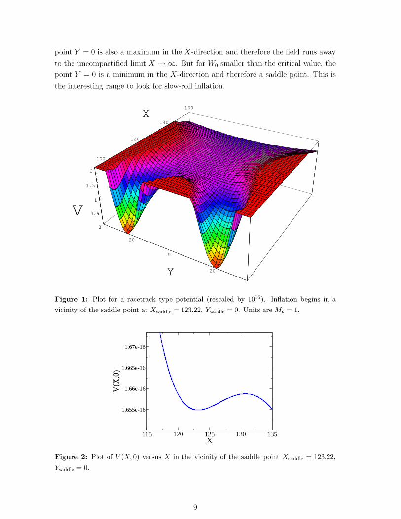
the interesting range to look for slow-roll inflation.

100

120

140

160

X

-20

0

20

Y

0

0.5

1

1.5

2

V0

0.5

1

1.5

Figure 1: Plot for a racetrack type potential (rescaled by 1016). Inflation begins in a

vicinity of the saddle point at Xsaddle = 123.22, Ysaddle = 0. Units are Mp = 1.

115 120 125 130 135X

1.655e-16

1.66e-16

1.665e-16

1.67e-16

V(X

,0)

Figure 2: Plot of V (X, 0) versus X in the vicinity of the saddle point Xsaddle = 123.22,

Ysaddle = 0.

9

Figs. 1-2 illustrate a region of the scalar potential for which inflation is possible.

The values of the parameters which are used to obtain this potential are:

A =1

50, B = −

35

1000, a =

2π

100, b =

2π

90, W0 = −

1

25000. (3.11)

With these values the two minima seen in the figure occur for field values

Xmin = 96.130, Ymin = ±22.146 , (3.12)

and the inflationary saddle point is at

Xsaddle = 123.22, Ysaddle = 0 . (3.13)

The value of E is fixed by demanding that the value of the potential at this

minimum be at zero, which turns out to require E = 4.14668 × 10−12. We find this

to be a reasonable value given that E is typically suppressed by the warp factor of

the metric at the position of the anti-brane.

It is crucial that this model contains two degenerate minima5 since this guar-

antees the existence of causally disconnected regions of space which are in different

vacua. These regions necessarily have a domain wall between them where the field

is near the saddle point and thus eternal inflation is taking place, provided that the

slow roll conditions (2.1) are satisfied there. It is then inevitable to have regions close

to the saddle in which inflation occurs, with a sufficiently large duration to explain

our flat and homogeneous universe.

3.3 Scaling Properties of the Model

It is easy to see from the potential (3.10) that we can obtain models with rescaled

values of the critical points for other choices of parameters, having the same features

of inflation. This can be done simply by rescaling their values in the following way,

a→ a/λ , b → b/λ , E → λ2E , (3.14)

and also

A→ λ3/2A , B → λ3/2B , W0 → λ3/2W0 , (3.15)

Under all these rescalings the potential does not change under condition that the

fields also rescale

X → λX , Y → λY , (3.16)

5Note that the potential is periodic with period 900, i. e. there is a set of two degenerate minima

at every Y = 900 n where n = 0, 1, 2, .... etc.

10

in which case the location of the extrema also rescale. One can verify that the values

of the slow-roll parameters ǫ and η do not change and also the amplitude of the

density perturbations δρρ

remains the same. It is important to take into account that

the kinetic term in this model is invariant under the rescaling, which is not the case

for canonically normalized fields.

Another property of this model is given by the following rescalings

a→ a/µ , b→ b/µ , E → E/µ , (3.17)

The potential and the fields also rescale

V → µ−3V , X → µX , Y → µY , (3.18)

Under these rescalings the values of the slow-roll parameters ǫ and η do not change

however, the amplitude of the density perturbations δρρ

scales as µ−3/2.

These two types of rescalings allow to generate many other models from the

known ones, in particular, change the positions of the minima or, if one is interested

in eternal inflation, one can easily change δρρ

keeping the potential flat.

3.4 Slow-Roll Inflation

We now display the slow-roll inflation, by examining field motion near the saddle

point which occurs between the two minima identified above. Near the saddle point

Xsaddle = 123.22, Ysaddle = 0, the potential takes the value Vsaddle = 1.655 ×

10−16. At this saddle point the potential has a maximum in the Y direction and a

minimum in the X direction, so the initial motion of a slowly-rolling scalar field is

in the Y direction.

We compute the slow-roll parameters near the top of the saddle, keeping in mind

the fact that Y does not have a canonical kinetic term. Given the Kahler potential

we find that the kinetic term for X and Y is

Lkin =3M2

p

4X2(∂µX∂

µX + ∂µY ∂µY ) (3.19)

and so the correctly normalized η parameter is given by the expression η = 2X2V ′′/3V ,

with X evaluated at the saddle point. We find in this way the slow-roll parameters

ǫsaddle = 0, ηsaddle = −0.006097 , (3.20)

given the values of the parameters taken above. The small size of η is very encourag-

ing given the reasonable range of parameters chosen. Recall from section 2 that the

11

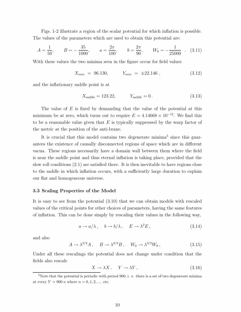
103A −103B − 10−3

Wmin− 10−3

Wmax

20 35 24.998 25.000

20 34 20.389 20.400

10 16 26.766 26.780

5 7.5 34.496 34.520

5 7 21.800 21.824

313

413

20.280 20.304

267

337

14.420 14.448

267

317

8.6884 8.708

−B −1/Wmin −1/Wmax

3.5 90685.8 90667.55

3.3 57273.9 57286.2

3.0 27371.1 27377.8

2.8 16111.8 16116.17

2.4 5009.38 5011.125

2.0 1301.6 1302.23

1.6 267.445 267.651

Table 1: A range of parameters chosen

to satisfy −0.05 < η < 0, close to the

parameter region (3.11).

Table 2: Another such range of parame-

ters, with a = π/5, b = 2π/9 and A = 1.

slow-roll condition η ≪ 1 being satisfied at the saddle point implies automatically

that we have an inflationary regime in its vicinity, and that inflation starting here is

an example of eternal topological inflation.

How fine-tuned is this parameter choice we have found which accomplishes in-

flation? Its success relies on the second derivative, ∂2V/∂Y 2, passing through a zero

very close to the saddle point (where ∂V/∂Y vanishes). Our ability to accomplish

this relies on the freedom to adjust W0, a parameter which is not present in a pure

racetrack model. To study the range of parameters which produce inflation we ex-

plored the vicinity of the parameters (3.11) which produce an inflationary solution.

We were able to preserve the condition −0.05 < η < 0 by varying the parameters W0

and B, while at all times adjusting E to keep the potential’s minimum at zero. For

many choices of B, sufficiently small η was obtained for Wmin < W0 < Wmax, given

in Table 1. The same is done in Table 2 for a different inflationary region of param-

eter space. We see from these tables that the success of slow-roll inflation typically

requires a fine tuning of parameters at the level of 1 part in 1000. Parameter values

in Table 1 were chosen so as to respect the COBE normalization (see below). This

constraint was not imposed for the values chosen in Table 2, but this can always be

compensated using the rescaling (3.17).

To compute observable quantities for the CMB we numerically evolve the scalar

field starting close to the saddle point, and let the fields evolve according to the

cosmological evolution equations for non-canonically normalized scalar fields [42, 15,

12

43, 44]:

ϕi + 3Hϕi + Γijk ϕ

j ϕk + gij ∂V

∂ϕj= 0 ,

H2 ≡

(

a

a

)2

=8πG

3

(

1

2gijϕ

iϕj + V

)

, (3.21)

where ϕi represent the scalar fields (ReT ≡ X and ImT ≡ Y in our case), a is the

scale factor (not to be confused with the exponent in the superpotential), and Γijk

are the target space Christoffel symbols using the metric gij for the set of real scalar

fields ϕi such that ∂2K∂ΦI∂ΦJ∗

∂ΦI∂Φ∗J = 12gij∂ϕ

i∂ϕj .

For numerical purposes it is more convenient to write the evolution of the fields

as a function of the number N of e-foldings rather than time. Using

a(t) = eN ,d

dt= H

d

dN, (3.22)

we avoid having to solve for the scale factor, instead directly obtaining X(N) and

Y (N). The equations of motion are

X ′′ = −

(

1 −X ′2 + Y ′2

4X2

)(

3X ′ + 2X2V,X

V

)

+X ′2 − Y ′2

X

Y ′′ = −

(

1 −X ′2 + Y ′2

4X2

)(

3Y ′ + 2X2V,Y

V

)

+ 2X ′Y ′

X(3.23)

where ′ denotes ddN

. The results of the numerical evolution are shown in figure 3 and 4,

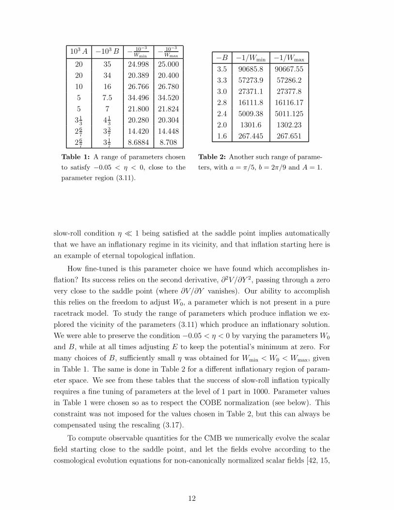
using the parameters (3.11) and the initial conditions X = Xsaddle (from (3.13)) and

Y = 0.1. Fig. 3 shows that this choice gives approximately 137 e-foldings of inflation

before the fields start oscillating around one of the local minima. Fig. 4 illustrates

that the inflaton is primarily Y at the very beginning of inflation, as must be the case

since Y is the unstable direction at the saddle point. Starting at Y = 0.2 would give

63 rather than 137 e-foldings of inflation. However, as it has already been explained,

tuning of initial conditions is not a concern within the present model, where inflation

is topological and eternal; all possible initial conditions will be present in the global

spacetime.

3.5 Experimental Constraints and Signatures

Let us now consider the experimental constraints on and predictions of the racetrack

inflation model. First, we must satisfy the COBE normalization on the power spec-

trum of scalar density perturbations,√

P (k) = 2× 10−5, at the scale k0 ∼ 103 Mpc,

or equivalently at the value of N which is approximately 60 e-foldings before the

13

136 137 138N (# of e-foldings)

0

20

40

60

80

100

120

fiel

d va

lues X(N)

Y(N)

5 10 15 20Y

95

100

105

110

115

120

X

Figure 3: Evolution of X (upper curve)

and Y (lower curve) from their initial val-

ues near the saddle point, to one of the

degenerate minima of the potential.

Figure 4: Path of inflaton trajectory in

X-Y field space.

end of inflation. We ignore isocurvature fluctuations (arising from fluctuations of the

fields orthogonal to the inflaton path shown in fig. 4) since there is always a hierarchy

between the second derivative of the potential along the path relative to that along

the orthogonal direction; then the magnitude of the scalar power spectrum can be

approximated by either

P1(k) =1

50π2

H4

Lkin

or P2(k) =1

150π2

V

ǫ(3.24)

where the generalization of the slow-roll parameter ǫ in the two-field case is given by

ǫ = M2p

(V,XX + V,Y Y )2

4Lkin V 2(3.25)

We have numerically checked that the two formulas give consistent results during the

slow-roll period, and that the COBE normalization is satisfied for the parameters

given in (3.11).

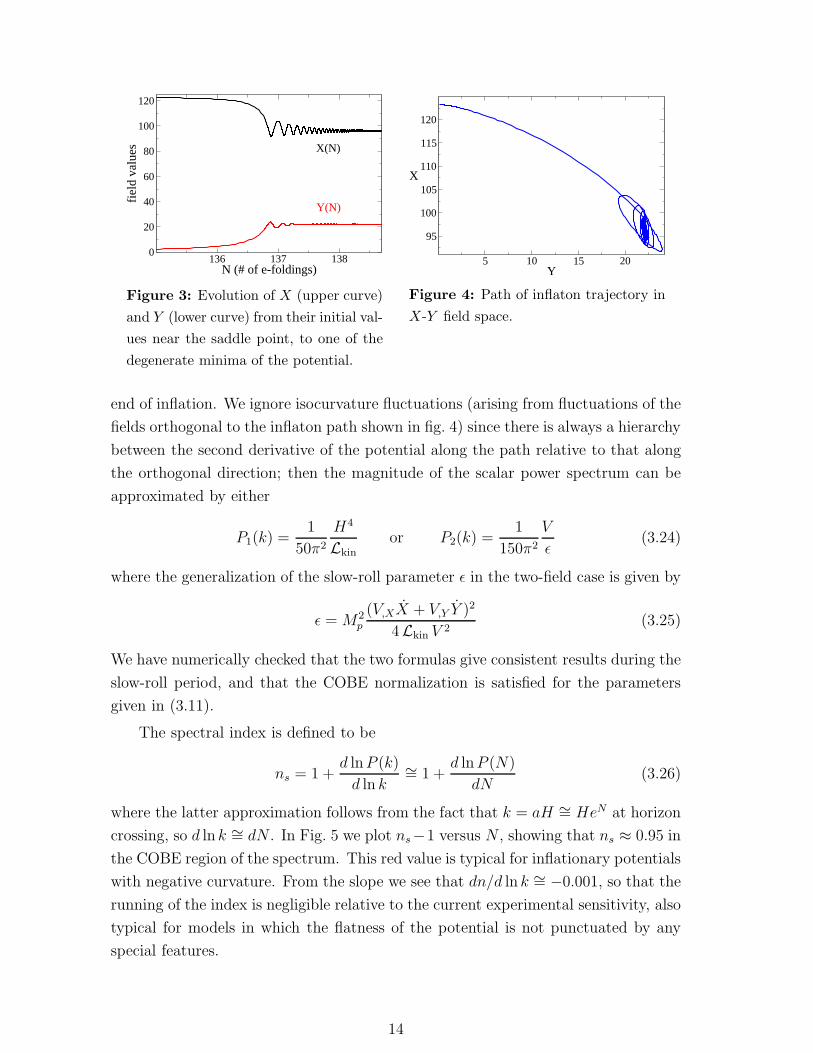
The spectral index is defined to be

ns = 1 +d lnP (k)

d ln k∼= 1 +

d lnP (N)

dN(3.26)

where the latter approximation follows from the fact that k = aH ∼= HeN at horizon

crossing, so d ln k ∼= dN . In Fig. 5 we plot ns−1 versus N , showing that ns ≈ 0.95 in

the COBE region of the spectrum. This red value is typical for inflationary potentials

with negative curvature. From the slope we see that dn/d ln k ∼= −0.001, so that the

running of the index is negligible relative to the current experimental sensitivity, also

typical for models in which the flatness of the potential is not punctuated by any

special features.

14

50 60 70 80 90 100 110N

-0.12

-0.1

-0.08

-0.06

-0.04

-0.02

(n-1

)

COBE

Figure 5: Deviation of the scalar power spectral index from 1 (n−1) versus N (equivalent

to n − 1 versus ln k) for the typical racetrack model.

The value of the spectral index ns ≈ 0.95 and the smallness of the running index

appear to be pretty stable with respect to various modifications of the model; we were

unable to alter these results by changing various parameters. This makes racetrack

inflation testable; at present, the best constraint on ns is ns = 0.98±0.02 [47], which

is compatible with our results. Future experiments will be able either confirm our

model or rule it out; in particular, Planck satellite will measure ns with accuracy

better than 0.01.

It is interesting that experimental tests will be able to discriminate for or against

the model in the not-too-distant future. The presence of a tensor contribution will

not provide any test in the example we have considered since the scale of inflation

is V 1/4 ∼ 1014 GeV, far below the 3 × 1016 GeV threshold needed for producing

observable gravity waves.

In order to formulate the theory of reheating in our scenario one needs to find

a proper way to incorporate the standard model matter fields in our model. In the

KKLT scenario there are two possible places where the standard model particles can

live: on (anti) D3 branes at the end of the throat [45] or on the wrapped D7 branes,

after some twisting and/or turning-on of magnetic fields. If the standard model

fields live on a D7 brane, the axion couples to the vector fields like Y FµνFµν and

the volume modulus as XFµνFµν . To study the reheating one has to find the decay

rate of the X and Y fields to the vector particles and the corresponding reheating

temperature. A preliminary investigation of this question along the lines of Ref. [46]

shows that reheating in this scenario can be rather efficient.6 Explicit models of this

6This situation will be the same in heterotic string realizations of our scenario (with the role

15

type are yet to be constructed. If the standard model is on D3 branes, we would

have to consider other couplings of the T -field to matter fields. We hope to return to

the theory of reheating in the racetrack inflation scenario in a separate publication.

4. The overshooting problem and initial conditions for the

racetrack inflation

Even though we already discussed advantages of eternal topological inflation from

the point of view of the problem of initial conditions, we will revisit this issue here

again, emphasizing specific features of eternal inflation in the context of string theory.

There is a well-known problem related to initial conditions in string cosmology

[48]. This problem, in application to the KKLT-based models, can be formulated

as follows. Even though there is a KKLT minimum of the potential with respect to

the dilaton field and the volume modulus X, this minimum is separated from the

global Minkowski minimum at X → ∞ by a relatively small barrier. The height

of the barrier depends on the parameters of the model, but in the simplest models

considered in the literature it is 10 to 20 orders of magnitude smaller than the Planck

density. In particular, for the parameters of our model, the height of the barrier is

2 × 10−16 in Planckian units, see Fig. 1. Generically, one could expect that soon

after the big bang, the energy density of all fields, including the field X, was many

orders of magnitude greater than the height of the barrier. If, for example, the field

X initially was very small, with energy density much larger than 2 × 10−16, then it

would fall down along the exponentially steep potential, easily overshoot the KKLT

minimum, roll over the barrier, and continue rapidly rolling towards X → ∞. This

would correspond to a rapid decompactification of the 4D space.

There are several ways to avoid this problem. One may try, for example, to

evaluate the possibility that instead of being born in a state with small X = Re T ,

the universe was created “from nothing” in a state corresponding to the inflationary

saddle point of the potential V (T ). This would resolve the problem of overshooting.

However, at the first glance, instead of solving the problem of initial conditions, this

only leads to its even sharper formulation.

Indeed, according to [49, 50], the probability of quantum creation of a closed

universe in a state corresponding to an extremum of its effective potential is given

by P ∼ exp(

− 24π2

V (T )

)

, where the energy density is expressed in units of the Planck

of the T field taken by the dilaton S) in which the dilaton field couples universally to hidden and

observable gauge fields.

16

density. The same expression appears for quantum creation of an open universe [51].

This leads to an alternative formulation of the problem of initial conditions in our

scenario: The probability that a closed (or open) universe is created from “nothing”

at the saddle point with V ∼ 2 × 10−16 is exponentially suppressed by the factor

of P ∼ exp (−1018). This result, taken at its face value, may look pretty upsetting.

(The simplest models of chaotic inflation, which can begin at V (φ) = O(1), do not

suffer from this problem [25].)

In Section 2 we outlined a possible resolution of this problem: Even if the proba-

bility of proper initial conditions for eternal topological inflation is extremely small,

the parts of the universe where these conditions are satisfied enter the regime of eter-

nal inflation, producing infinite amount of homogeneous space where life of our type

is possible. Thus, even if the fraction of the universes (or of the parts of our universe)

with inflationary initial conditions is exponentially suppressed, one may argue that

eventually most of the observers will live in the parts of the universe produced by

eternal topological inflation.

Here we would like to strengthen this argument even further, by finding the

conditions which may allow us to remove the exponential suppression of the prob-

ability of initial conditions for the low energy scale inflation. In order to do it, let

us identify the root of the problem of the exponential suppression: At the classical

level, the minimal size of a closed de Sitter space is H−1. Quantum creation of a

closed inflationary universe is described by the tunneling from the state with the

scale factor a = 0 (no universe) to the state where the size of the universe becomes

equal to its minimal value a = H−1(T ). Exponential suppression appears because of

the large absolute value of the Euclidean action on the tunneling trajectory [49, 50].

One could expect that for an open universe there is no need for tunneling because

there is no barrier for the classical evolution of an open universe from a = 0 to

larger a. However, an instant creation of an infinite homogeneous open universe is

problematic (homogeneity and horizon problems). The only known way to describe

it is to use a different analytic continuation of the same instantons that were used

for the description of quantum creation of a closed universe [52], which again leads

to the exponential suppression of the probability [51].

Fortunately, there is a simple way to overcome this problem [53], which is directly

related to the standard Kaluza-Klein picture of compactification in string theory. In

this picture, it is natural to assume that all spatial dimensions enter the theory

democratically, i.e. all of them are compact, not necessarily because of the curvature

of space (as in the closed universe case), but because of its nontrivial topology. Then

inflation makes the size of 3 of these dimensions exponentially large, whereas the size

17

of 6 other dimensions remains fixed, e.g., by the KKLT mechanism.

For example, one may consider a toroidal compactification of a flat universe,

or compactification of an open universe. This is a completely legitimate possibility,

which was investigated by many authors; see e.g. [54, 55, 56, 57]. It does not

contradict any observational data if inflation is long enough to make the size of the

universe much greater than 1010 light years.

An important feature of a topologically nontrivial compact flat or open dS space

is that (ignoring the Casimir effect which is suppressed by supersymmetry) its classi-

cal evolution can continuously proceed directly from the state with a(t) → 0, without

any need of tunneling, unlike in the closed universe case [58]. As a result, there is

no exponential suppression of the probability of quantum creation of a compact flat

or open inflationary universe with V (T ) ≪ 1 [53]. This observation removes the

main objection against the possibility of the low energy scale inflation starting at an

extremum of the effective potential.

Moreover, in an eternally inflating universe consisting of many de Sitter parts

corresponding to the string theory landscape, the whole issue of initial conditions

should be formulated in a different way [27, 59]. In such a universe, inflation is

always eternal because of the incomplete decay of metastable dS space, as in old

inflation. Therefore evolution of such a universe will produce infinitely large number

of exponentially large parts of the universe with different properties [27, 62]. Even if

in many of such parts space will become 10D after the scalar field T overshoots the

KKLT barrier, this will be completely irrelevant for the evolution of other parts of the

universe where space remains 4D. In some parts of 4D space there was no inflation,

and adiabatic perturbations with a flat spectrum could not be produced. Even

though such parts initially may be quite abundant, later on they do not experience

an additional inflationary growth of their volume. Observations tell us that we do not

live in one of such parts. Meanwhile inflationary trajectories starting at the saddle

point describe eternally inflating parts of the universe which produce an indefinitely

large volume of homogeneous 4D space where observers of our type can live. This

observation goes long way towards resolving the problem of initial conditions in our

scenario.

5. Irrational Racetrack Inflation and the Cosmological Con-

stant

In order to achieve a successful cosmological scenario, one needs to make at least two

18

fine-tunings. First of all, we must fine-tune the uplifting of the AdS potential in the

KKLT scenario to obtain the present value of the cosmological constant Λ ∼ 10−120

in units of Planck density. Then we must fine-tune the parameters of our model

in order to achieve a slow-roll inflation with the amplitude of density perturbationsδρρ∼ 10−5.

One way to approach the fine-tuning problem is to say that the smallness of

the cosmological constant, as well as the stage of inflation making our universe large

and producing small density perturbations are necessary for the existence of life as

we know it. This argument may make sense in the context of the eternal inflation

scenario, but only if there are sufficiently many vacuum states with different values of

the cosmological constant, and one can roll down to these states along many different

inflationary trajectories.

In this respect, the possibility that the eternally inflating universe becomes di-

vided into many exponentially large regions with different properties [25, 60] and

the related idea of the string theory landscape describing enormously large number

of different vacua may be very helpful [61, 62, 35]. However, even in this case one

must check whether the set of parameters which are possible in string theory is dense

enough to describe theories with Λ ∼ 10−120 and δρρ∼ 10−5.

80 100 120 140

-40

-20

0

20

40

80 100 120 140

860

880

900

920

940

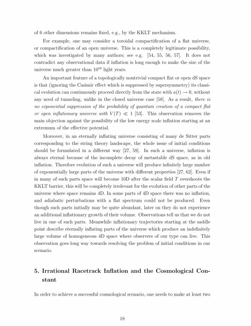
Figure 6: Contour plot of the effective potential in the vicinity of the saddle point at

Y = 0 (left panel) and at Y ∼ 900 (right panel).

One way towards making the choice of various vacua infinitely rich is related to

the irrational axion scenario [63]. In our previous discussion of the effective potential

of our model, Eq. (3.10), we assumed that a = 2πM

and b = 2πN

, where N and M

are integers. In this case the potential is periodic in Y , with a period MN , or less,

19

MN/(M−N) if M/(M−N) and N/(M−N) are integers. For example, if one takes

M = 100 and N = 90, the potential will have identical inflationary saddle points for

all Y = n(MN/(M −N)) = 900n, where n is an arbitrary integer.

However, if one assumes that instead of being an integer, at least one of the

numbers M , N is irrational, then in the infinitely large interval of all possible values

of the axion field Y values one would always find vacua with all values of Λ varying

on a very large scale comparable with the height of the potential barrier in the KKLT

potential. Similarly, if we, for example, start with an irrational number M very close

to 1000, then at Y = 0 we will have the same scenario as in the model described

above, but at large Y we will have all kinds of extrema and saddle points, leading to

various stages of inflation with different amplitude of density perturbations.

To illustrate this idea, we give here the contour plots of two subsequent saddle

points which appear in our theory under a very mild modification: We replace M =

100 by M = 100+ π100

. It immediately produces an infinitely large variety of different

shape saddle points and minima of different depth; we show two different saddle

points separated by Y ≈ 900 in Fig. 6. The shape and the depth of the minima

of these potentials can be changed in an almost continuous way. This reflects the

situation with irrational winding line on the torus for incommensurate frequencies:

the system will never return to its original position, it will cover the torus densely,

coming arbitrary close to every point.

The main question is whether one can find a version of string theory with the

superpotential involving irrational M . Whereas no explicit examples of such models

are known at present, the idea is so attractive that we allow ourselves to speculate

about its possible realizations. One can try to use the setting of [64] where the non-

commutative solitons on orbifolds are studied and some relation to irrational axions

is pointed out. One can also look for the special contribution to the Chern-Simons

term on D7 due to the 2-form fluxes. The standard aFF ∗ axion coupling originates

from the term∫

M9 d[CeF ] where one finds d[CeF ] ∼ da ∧ F ∧ F ∧ J ∧ J and J is

the Kahler form and da ∧ J ∧ J comes from the self-dual five-form. Perhaps it is

not impossible to find in addition to this term a contribution where one or both of

the Kahler forms are replaced by the 2-form fluxes F = F − B. Here the 2-form B

is not quantized and is related to the non-commutativity parameter in the internal

space. This may lead to some new coupling of the form qaFF ∗ where q is irrational

as proposed in [63].

20

6. Conclusions

We present what we believe is the simplest model for inflation in a string-theoretic

scenario. It requires a certain amount of fine-tuning of the parameters of the non-

perturbative racetrack superpotential. Inflation only occurs due to the existence of

a nontrivial potential lifting the complex Kahler structure modulus whose real part

is the overall size of the compact space and the imaginary part coming from the

type IIB four-form is the inflaton field. The periodicity properties in this direction

make the scalar potential very rich and we find explicit configurations realizing the

slow-roll/topological inflation setting that give rise to eternal inflation and density

perturbations in our patch consistent with the COBE normalization and spectral

index inside (but close to the edge of) the current observational bounds. We find

this to be very encouraging.

It is appropriate to compare our scenario with the other direction for obtaining

inflation in string theory, namely the brane/brane [6, 10] or brane/antibrane [7, 8]

inflationary scenarios in which the inflaton field corresponds to the separation of the

branes ψ and inflation ends by the appearance of an open string tachyon in a stringy

realization of hybrid inflation [7, 10]. Clearly our racetrack scenario is much simpler

since there is no need to introduce the brane configurations with their separation

field ψ to obtain inflation. The analysis of [13] pointed out the difficulty in obtaining

brane inflation once a mechanism for moduli fixing is included. Various extensions

and improvements of the basic scenario were considered in [13, 15, 16], they typically

require a fine-tuning. At present only D3/D7 brane inflation model compactified on

K3 × T2

Z2with volume stabilization does not seem to require a fine-tuning [65].

In addition, in brane inflation scenario the tachyon potential can give rise to

topological defects such as cosmic strings [7, 13, 66] which may have important ob-

servational implications [66, 67]. Furthermore, having an implementation of inflation

in string theory, independent of brane inflation, diminishes in some sense the possible

observational relevance of cosmic strings as being a generic implication of the brane

inflation scenario. In racetrack inflation, cosmic strings need not be generated after

inflation.

On the other hand there is no inconsistency to combine both scenarios. For

instance, in realistic generalizations of the KKLT scenario including standard model

branes [45], the throat where the standard model lives should be significantly warped,

whereas brane/antibrane inflation required a mild warping in the inflation throat in

order to be consistent with the COBE normalization [15]. Also the fine tuning

involved suggested two or more stages of inflation with some 20-30 e-foldings at

21

a high scale and the rest at a small scale, probably close to 1 TeV. This, besides

having interesting observational implications, may also help to the solution of the

cosmological moduli problem [68] which usually needs a late period of inflation. We

could then foresee a scenario in which racetrack inflation is at work at high scales

and the low-scale inflation is provided by brane/antibrane collision in the standard

model throat. See [69] for a previous discussion of low-scale inflation.

There are many avenues along which to generalize our approach. Modular infla-

tion could also be obtained by using more general modular superpotentials than those

of the racetrack type considered here. Also, potentials for many moduli fields are

only starting to be explored and some of them have the advantage that a nonvanish-

ing superpotential has been obtained [35]. It would also be interesting to investigate

if the irrational cases proposed here are actually obtainable from string theory. We

hope to report on some of these issues in the future.

7. Acknowledgements

We would like to thank R. Brustein, E. Copeland, S. P. de Alwis, G. Dvali, A.

Font, S. Gratton, A. Gruzinov, A. Iglesias, X. de la Ossa, L. Ibanez, S. Kachru, N.

Kaloper, G. Ross, S. Sarkar, R. Scoccimarro, E. Silverstein, H. Tye and A. Vilenkin

for useful conversations. We also thank the organizers of the ‘New Horizons in String

Cosmology’ workshop at the Banff International Research Station for providing the

perfect environment for completing this work and for contemplating the landscape.

C.B. and J.C. are funded by grants from NSERC (Canada), NATEQ (Quebec) and

McGill University. The work of M.G.-R. is supported by D.O.E. under grant DE-

FG02-92ER40706. J.J.B-P. is supported by the James Arthur Fellowship at NYU.

C.E. is partially funded by EPSRC. The work of R.K. and A.L. is supported by the

NSF (US) grant 0244728. F.Q. is partially funded by PPARC and a Royal Society

Wolfson award.

References

[1] P. Binetruy and M. K. Gaillard, “Candidates For The Inflaton Field In Superstring

Models,” Phys. Rev. D 34 (1986) 3069.

[2] T. Banks, M. Berkooz, S. H. Shenker, G. W. Moore and P. J. Steinhardt, “Modular

cosmology,” Phys. Rev. D 52 (1995) 3548 [arXiv:hep-th/9503114].

[3] J. P. Derendinger, L. E. Ibanez and H. P. Nilles, “On The Low-Energy D = 4, N=1

Supergravity Theory Extracted From The D = 10, N=1 Superstring,” Phys. Lett. B

22

155 (1985) 65; M. Dine, R. Rohm, N. Seiberg and E. Witten, “Gluino Condensation

In Superstring Models,” Phys. Lett. B 156 (1985) 55;

[4] N.V. Krasnikov, “On Supersymmetry Breaking In Superstring Theories,” PLB 193

(1987) 37; L.J. Dixon, ”Supersymmetry Breaking in String Theory”, in The Rice

Meeting: Proceedings, B. Bonner and H. Miettinen eds., World Scientific (Singapore)

1990; T.R. Taylor, ”Dilaton, Gaugino Condensation and Supersymmetry Breaking”,

PLB252 (1990) 59 B. de Carlos, J. A. Casas and C. Munoz, “Supersymmetry

breaking and determination of the unification gauge coupling constant in string

theories,” Nucl. Phys. B 399 (1993) 623 [arXiv:hep-th/9204012].

[5] A. Font, L. E. Ibanez, D. Lust and F. Quevedo, “Supersymmetry Breaking From

Duality Invariant Gaugino Condensation,” Phys. Lett. B 245 (1990) 401; S. Ferrara,

N. Magnoli, T. R. Taylor and G. Veneziano, “Duality And Supersymmetry Breaking

In String Theory,” Phys. Lett. B 245 (1990) 409; M. Cvetic, A. Font, L. E. Ibanez,

D. Lust and F. Quevedo, “Target space duality, supersymmetry breaking and the

stability of classical string vacua,” Nucl. Phys. B 361 (1991) 194.

[6] G. R. Dvali and S. H. H. Tye, “Brane inflation,” Phys. Lett. B 450 (1999) 72

[arXiv:hep-ph/9812483].

[7] C. P. Burgess, M. Majumdar, D. Nolte, F. Quevedo, G. Rajesh and R. J. Zhang,

“The inflationary brane-antibrane universe,” JHEP 0107 (2001) 047

[arXiv:hep-th/0105204].

[8] G. R. Dvali, Q. Shafi and S. Solganik, “D-brane inflation,” arXiv:hep-th/0105203.

[9] C. P. Burgess, P. Martineau, F. Quevedo, G. Rajesh and R. J. Zhang, “Brane

antibrane inflation in orbifold and orientifold models,” JHEP 0203 (2002) 052

[arXiv:hep-th/0111025].

[10] C. Herdeiro, S. Hirano and R. Kallosh, “String theory and hybrid inflation /

acceleration,” JHEP 0112 (2001) 027 [arXiv:hep-th/0110271]; K. Dasgupta,

C. Herdeiro, S. Hirano and R. Kallosh, “D3/D7 inflationary model and M-theory,”

Phys. Rev. D 65 (2002) 126002 [arXiv:hep-th/0203019].

[11] J. Garcia-Bellido, R. Rabadan and F. Zamora, “Inflationary scenarios from branes at

angles,” JHEP 0201, 036 (2002); N. Jones, H. Stoica and S. H. H. Tye, “Brane

interaction as the origin of inflation,” JHEP 0207, 051 (2002); M. Gomez-Reino and

I. Zavala, “Recombination of intersecting D-branes and cosmological inflation,” JHEP

0209, 020 (2002).

[12] For reviews with many references see: F. Quevedo, Class. Quant. Grav. 19 (2002)

5721, [arXiv:hep-th/0210292]; A. Linde, “Prospects of inflation,”

[arXiv:hep-th/0402051].

23

[13] S. Kachru, R. Kallosh, A. Linde, J. Maldacena, L. McAllister and S. P. Trivedi,

“Towards inflation in string theory,” JCAP 0310 (2003) 013 [arXiv:hep-th/0308055].

[14] J. P. Hsu, R. Kallosh and S. Prokushkin, “On brane inflation with volume

stabilization,” JCAP 0312 (2003) 009 [arXiv:hep-th/0311077]; F. Koyama,

Y. Tachikawa and T. Watari, “Supergravity analysis of hybrid inflation model from

D3-D7 system”, [arXiv:hep-th/0311191]; H. Firouzjahi and S. H. H. Tye, “Closer

towards inflation in string theory,” Phys. Lett. B 584 (2004) 147

[arXiv:hep-th/0312020]. J. P. Hsu and R. Kallosh, “Volume stabilization and the

origin of the inflaton shift symmetry in string theory,” JHEP 0404 (2004) 042

[arXiv:hep-th/0402047];

[15] C. P. Burgess, J. M. Cline, H. Stoica and F. Quevedo, “Inflation in realistic D-brane

models,” [arXiv:hep-th/0403119].

[16] O. DeWolfe, S. Kachru and H. Verlinde, “The giant inflaton,” JHEP 0405 (2004)

017 [arXiv:hep-th/0403123]; N. Iizuka and S. P. Trivedi, “An inflationary model in

string theory,” arXiv:hep-th/0403203; A. Buchel and A. Ghodsi, “Braneworld

inflation,” arXiv:hep-th/0404151.

[17] S. Kachru, R. Kallosh, A. Linde and S. P. Trivedi, “De Sitter vacua in string

theory,” Phys. Rev. D 68 (2003) 046005 [arXiv:hep-th/0301240].

[18] See for instance: E. J. Copeland, A. R. Liddle, D. H. Lyth, E. D. Stewart and

D. Wands, “False vacuum inflation with Einstein gravity,” Phys. Rev. D 49 (1994)

6410 [astro-ph/9401011].

[19] C. Escoda, M. Gomez-Reino and F. Quevedo, “Saltatory de Sitter string vacua,”

JHEP 0311 (2003) 065 [arXiv:hep-th/0307160].

[20] A. D. Linde, “Monopoles as big as a universe,” Phys. Lett. B 327, 208 (1994)

[arXiv:astro-ph/9402031]; A. D. Linde and D. A. Linde, “Topological defects as seeds

for eternal inflation,” Phys. Rev. D 50, 2456 (1994) [arXiv:hep-th/9402115].

[21] A. Vilenkin, “Topological inflation,” Phys. Rev. Lett. 72, 3137 (1994).

[22] K. Freese, J. A. Frieman and A. V. Olinto, “Natural Inflation With Pseudo -

Nambu-Goldstone Bosons,” Phys. Rev. Lett. 65, 3233 (1990); F. C. Adams,

J. R. Bond, K. Freese, J. A. Frieman and A. V. Olinto, “Natural inflation: Particle

physics models, power law spectra for large scale structure, and constraints from

COBE,” Phys. Rev. D 47 (1993) 426 [arXiv:hep-ph/9207245].

[23] A. D. Linde, “Initial Conditions For Inflation,” Phys. Lett. B 162 (1985) 281.

24

[24] H. V. Peiris et al., “First year Wilkinson Microwave Anisotropy Probe (WMAP)

observations: Implications for inflation,” Astrophys. J. Suppl. 148, 213 (2003)

[astro-ph/0302225].

[25] A.D. Linde, Particle Physics and Inflationary Cosmology (Harwood, Chur,

Switzerland, 1990).

[26] A. D. Linde, “Eternally Existing Selfreproducing Chaotic Inflationary Universe,”

Phys. Lett. B 175, 395 (1986).

[27] A. D. Linde, D. A. Linde and A. Mezhlumian, “From the Big Bang theory to the

theory of a stationary universe,” Phys. Rev. D 49, 1783 (1994) [arXiv:gr-qc/9306035].

[28] P. J. Steinhardt, “Natural Inflation,” In: The Very Early Universe, ed. G.W.

Gibbons, S.W. Hawking and S.Siklos, Cambridge University Press, (1983);

A. D. Linde, “Nonsingular Regenerating Inflationary Universe,” Cambridge

University preprint Print-82-0554 (1982); A. Vilenkin, “The Birth Of Inflationary

Universes,” Phys. Rev. D 27, 2848 (1983).

[29] S. B. Giddings, S. Kachru and J. Polchinski, “Hierarchies from fluxes in string

compactifications,” Phys. Rev. D66, 106006 (2002).

[30] S. Sethi, C. Vafa and E. Witten, “Constraints on low-dimensional string

compactifications,” Nucl. Phys. B 480 (1996) 213 [arXiv:hep-th/9606122];

K. Dasgupta, G. Rajesh and S. Sethi, “M theory, orientifolds and G-flux,” JHEP

9908 (1999) 023 [arXiv:hep-th/9908088].

[31] E. Cremmer, S. Ferrara, C. Kounnas and D.V. Nanonpoulos, “Naturally vanishing

cosmological constant in N = 1 supergravity,” Phys. Lett. B133, 61 (1983); J. Ellis,

A.B. Lahanas, D.V. Nanopoulos and K. Tamvakis, “No-scale Supersymmetric

Standard Model,” Phys. Lett. B134, 429 (1984).

[32] C. P. Burgess, R. Kallosh and F. Quevedo, “de Sitter string vacua from

supersymmetric D-terms,” JHEP 0310 (2003) 056 [arXiv:hep-th/0309187].

[33] R. Brustein and S. P. de Alwis, “Moduli potentials in string compactifications with

fluxes: Mapping the discretuum,” Phys. Rev. D 69, 126006 (2004)

[arXiv:hep-th/0402088]; A. Saltman and E. Silverstein, “The scaling of the no scale

potential and de Sitter model building,” hep-th/0402135.

[34] L. Gorlich, S. Kachru, P. Tripathy and S. Trivedi, “Gaugino Condensation and

Nonperturbative Superpotentials in F-theory,” to appear.

[35] F. Denef, M. R. Douglas and B. Florea, “Building a better racetrack,” JHEP 0406

(2004) 034 [arXiv:hep-th/0404257].

25

[36] D. Robbins and S. Sethi, “A barren landscape,” arXiv:hep-th/0405011.

[37] C.P. Burgess, J.-P. Derendinger, F. Quevedo and M. Quiros, “Gaugino Condensates

and Chiral-Linear Duality: An Effective-Lagrangian Analysis”, Phys. Lett. B 348

(1995) 428–442; “On Gaugino Condensation with Field-Dependent Gauge Couplings”,

Ann. Phys. 250 (1996) 193-233.

[38] C.P. Burgess, A. de la Macorra, I. Maksymyk and F. Quevedo, “Supersymmetric

Models with Product Gauge Groups and Field Dependent Gauge Couplings,” JHEP

9809 (1998) 007 (30 pages) (hep-th/9808087).

[39] E. Cremmer, B. Julia, J. Scherk, S. Ferrara, L. Girardello and P. van Nieuwenhuizen,

“Spontaneous Symmetry Breaking And Higgs Effect In Supergravity Without

Cosmological Constant,” Nucl. Phys. B 147, 105 (1979).

[40] E. Witten, “Dimensional Reduction Of Superstring Models,” Phys. Lett. B 155

(1985) 151; C. P. Burgess, A. Font and F. Quevedo, “Low-Energy Effective Action

For The Superstring,” Nucl. Phys. B 272 (1986) 661.

[41] S. Kachru, J. Pearson and H. Verlinde, “Brane/Flux Annihilation and the String

Dual of a Supersymmetric Field Theory,” JHEP 0206, 021 (2002), hep-th/0112197.

[42] R. Kallosh, A. Linde, S. Prokushkin and M. Shmakova, “Supergravity, dark energy

and the fate of the universe,” Phys. Rev. D 66, 123503 (2002) [arXiv:hep-th/0208156].

[43] R. Kallosh and S. Prokushkin, “Supercosmology,” arXiv:hep-th/0403060.

[44] C.P. Burgess, P. Grenier and D. Hoover, JCAP 0403 (2004) 008 (27 pages)

(hep-ph/0308252).

[45] J. F. G. Cascales, M. P. Garcia del Moral, F. Quevedo and A. M. Uranga, “Realistic

D-brane models on warped throats: Fluxes, hierarchies and moduli stabilization,”

JHEP 0402 (2004) 031 [arXiv:hep-th/0312051].

[46] L. Kofman, A. D. Linde and A. A. Starobinsky, “Towards the theory of reheating

after inflation,” Phys. Rev. D 56, 3258 (1997) [arXiv:hep-ph/9704452].

[47] U. Seljak et al., “Cosmological parameter analysis including SDSS Ly-alpha forest

and galaxy bias: Constraints on the primordial spectrum of fluctuations, neutrino

mass, and dark energy,” arXiv:astro-ph/0407372.

[48] R. Brustein and P. J. Steinhardt, “Challenges For Superstring Cosmology,” Phys.

Lett. B 302, 196 (1993) [arXiv:hep-th/9212049].

[49] A. D. Linde, “Quantum Creation Of The Inflationary Universe,” Lett. Nuovo Cim.

39, 401 (1984).

26

[50] A. Vilenkin, “Quantum Creation Of Universes,” Phys. Rev. D 30 (1984) 509.

[51] A. D. Linde, “Quantum creation of an open inflationary universe,” Phys. Rev. D 58,

083514 (1998) [arXiv:gr-qc/9802038].

[52] S. W. Hawking and N. Turok, “Open inflation without false vacua,” Phys. Lett. B

425, 25 (1998) [arXiv:hep-th/9802030].

[53] A. Linde, “Can we have inflation with Ω > 1?,” JCAP 0305, 002 (2003)

[arXiv:astro-ph/0303245]; A. Linde, to be published.

[54] D.D. Sokolov and V.F. Shvartsman, Sov. Phys. JETP 39, (1975) 196; G. Paal, Acta.

Phys. Acad. Scient. Hungaricae 30, (1971) 51; J.R. Gott, Mon. Not. R. Astron. Soc.

193 (1980) 153.

[55] D. D. Sokolov and A. A. Starobinsky, Sov. Astron. 19 (1976) 629; J. Levin,

E. Scannapieco and J. Silk, “The topology of the universe: the biggest manifold of

them all,” Class. Quant. Grav. 15, 2689 (1998) [arXiv:gr-qc/9803026]; J. Levin,

“Topology and the cosmic microwave background,” Phys. Rept. 365, 251 (2002)

[arXiv:gr-qc/0108043]; N. J. Cornish, D. N. Spergel, G. D. Starkman and E. Komatsu,

“Constraining the Topology of the Universe,” Phys. Rev. Lett. 92, 201302 (2004)

[arXiv:astro-ph/0310233]; A. Riazuelo, J. Weeks, J. P. Uzan, R. Lehoucq and

J. P. Luminet, “Cosmic microwave background anisotropies in multi-connected flat

spaces,” Phys. Rev. D 69, 103518 (2004) [arXiv:astro-ph/0311314].

[56] R. H. Brandenberger and C. Vafa, Nucl. Phys. B 316, 391 (1989).

[57] N. J. Cornish, D. N. Spergel and G. D. Starkman, “Does chaotic mixing facilitate

Ω < 1 inflation?,” Phys. Rev. Lett. 77, 215 (1996) [arXiv:astro-ph/9601034].

[58] Y. B. Zeldovich and A. A. Starobinsky, “Quantum Creation Of A Universe In A

Nontrivial Topology,” Sov. Astron. Lett. 10 (1984) 135.

[59] A. Linde, “Prospects of inflation,” arXiv:hep-th/0402051.

[60] A. Linde, “Inflation, quantum cosmology and the anthropic principle,” in Science

and Ultimate Reality: From Quantum to Cosmos (eds. J.D. Barrow, P.C.W. Davies,

and C.L. Harper, Cambridge University Press 2003). [arXiv:hep-th/0211048].

[61] R. Bousso and J. Polchinski, “Quantization of four-form fluxes and dynamical

neutralization of the cosmological constant,” JHEP 0006 (2000) 006.

[62] L. Susskind, “The anthropic landscape of string theory,” hep-th/0302219.

[63] W. A. Bardeen, S. Elitzur, Y. Frishman and E. Rabinovici, “Fractional Charges:

Global And Local Aspects,” Nucl. Phys. B 218, 445 (1983); T. Banks, M. Dine and

27

N. Seiberg, “Irrational axions as a solution of the strong CP problem in an eternal

universe,” Phys. Lett. B 273, 105 (1991) [arXiv:hep-th/9109040].

[64] E. J. Martinec and G. W. Moore, “Noncommutative solitons on orbifolds,”

arXiv:hep-th/0101199.

[65] S. Kachru, R. Kallosh and A. Linde, “String Inflation Update”, Work in progress.

[66] S. Sarangi and S. H. H. Tye, “Cosmic string production towards the end of brane

inflation,” Phys. Lett. B 536 (2002) 185 [arXiv:hep-th/0204074].

[67] G. Dvali, R. Kallosh and A. Van Proeyen, “D-term strings,” JHEP 0401 (2004) 035

[arXiv:hep-th/0312005]; G. Dvali and A. Vilenkin, “Formation and evolution of

cosmic D-strings,” JCAP 0403 (2004) 010 [arXiv:hep-th/0312007]; E. J. Copeland,

R. C. Myers and J. Polchinski, “Cosmic F- and D-strings,” JHEP 0406 (2004) 013

[arXiv:hep-th/0312067]; L. Leblond and S. H. H. Tye, “Stability of D1-strings inside a

D3-brane,” JHEP 0403 (2004) 055 [arXiv:hep-th/0402072]; K. Dasgupta, J. P. Hsu,

R. Kallosh, A. Linde and M. Zagermann, “D3/D7 brane inflation and semilocal

strings,” arXiv:hep-th/0405247.

[68] G. D. Coughlan, W. Fischler, E. W. Kolb, S. Raby and G. G. Ross, “Cosmological

Problems For The Polonyi Potential,” Phys. Lett. B 131 (1983) 59; T. Banks,

D. B. Kaplan and A. E. Nelson, “Cosmological implications of dynamical

supersymmetry breaking,” Phys. Rev. D 49 (1994) 779 [arXiv:hep-ph/9308292]; B. de

Carlos, J. A. Casas, F. Quevedo and E. Roulet, “Model independent properties and

cosmological implications of the dilaton and moduli sectors of 4-d strings,” Phys.

Lett. B 318 (1993) 447 [arXiv:hep-ph/9308325].

[69] J. A. Adams, G. G. Ross and S. Sarkar, “Multiple inflation,” Nucl. Phys. B 503

(1997) 405 [arXiv:hep-ph/9704286]; G. German, G. G. Ross and S. Sarkar,

“Implementing quadratic supergravity inflation,” Phys. Lett. B 469 (1999) 46

[arXiv:hep-ph/9908380]; “Low-scale inflation,” Nucl. Phys. B 608 (2001) 423

[arXiv:hep-ph/0103243].

28