MPRAMunich Personal RePEc Archive

Regional Inflation in China

Nagayasu, Jun

December 2009

Online at http://mpra.ub.uni-muenchen.de/24722/

MPRA Paper No. 24722, posted 31. August 2010 / 00:24

Regional In�ation in China

Jun Nagayasu�

University of Tsukuba

Dec 2009

Abstract

This paper empirically examines developments in price and in�ation in China

from 1991 to 2005. Unlike most previous studies, their determinants were inves-

tigated in the panel data context, and our �ndings are as follows. First, using

the panel cointegration method, we con�rm a long-run relationship between

price, money and output. Secondly, we provide evidence that in�ation can be

explained by economic fundamentals such as money, credits, productivity, and

exchange rate growth. Furthermore, while an increased concern about regional

discrepancies in recent years, this relationship is more sensitive to the sample

period than to the region type. Notably, money does not seem to be closely

associated with in�ation over recent years.

JEL classi�cation: E310, E500, R110

Keywords: China, in�ation, panel data, panel cointegration

�Mailing address: University of Tsukuba, Department of Social Systems and Management, 1-1-1Tennodai, Ibaraki 305-8573 JAPAN. Email: Nagayasu@sk.tsukuba.ac.jp. An earlier version of thispaper was presented at the 83rd Annual Conference of the Western Economic Association Inter-national (Honolulu 2008) and the Fall Conference of the Japanese Society of Monetary Economics(Hiroshima 2008). I would like to thank Zipei Chen and Ying Shen for data collection. I also thankfor useful comments Gregory Givens, Akihiro Kubo, Ying Liu, Robert J. Sonora, Qing Yuan Sui,Yonghong Tu, and conference participants. This research was partly �nanced by the Data BankProject at Tsukuba University. However, all errors remain mine.

1

1 Introduction

Over recent years, China has experienced high economic growth with relatively mod-

erate in�ation by international standards. Its annual GDP growth rate has often

exceeded 10 percent with a peak of around 35 percent in the mid 1990s. Because

many developed countries have experienced slow economic growth since 1990, China

has often been claimed as the engine of the world economy.

Figure 1 shows the Chinese GDP growth (measured in local currency), Chinese

in�ation, and world average in�ation rates from 1991 to 2005. This suggests that the

Chinese in�ation rate was generally lower than its GDP growth and the world in�ation

rate, and actually experienced de�ation in the second half of the 1990s and early

2000s. The low in�ation relative to GDP is consistent with China�s macroeconomic

policy since the �ve-year economic plan often makes reference to this as one of its

economic targets. The moderate in�ation rate was argued as resulting from several

factors including a strong supply side owing to the cheap labor force and periodic weak

demand for consumer goods.1

However, in the last couple of years, the sustainability of this economic growth

has been brought into question since cheap labor is no longer available, and there is

considerable upward pressure on wages and in�ation. More recently, considerable con-

struction for the 2008 Beijing Olympics as well as soaring commodity (e.g., wheat and

oil) prices worldwide have become additional factors contributing to the increased in-

�ationary pressure. While the adverse e¤ects of the sub-prime loan crisis have became

apparent worldwide in the second half of 2008 and subdued in�ationary pressure, it

began to increase again in China in 2009 along with world economic recovery.

In�ation increases in China have major policy implications for both domestic and

international economies. Amongst other possibilities, high in�ation may have a dele-

terious e¤ect on future Chinese economic growth, resulting in higher wages, more

expensive exports, and fewer foreign reserves. Moreover, due to the high volume of

exported goods, more expensive exports from China might increase in�ation overseas

also. Thus, it has become a pressing research topic in many countries.

Among many others, pertinent previous studies include Huang (1994), Girardin

(1996), Chen (1997), Hasan (1999), Gerlach and Peng (2006), Funke (2006), and

Burdekin and Siklos (2006). Using country-level data, Huang (1994) and Chen (1997)

con�rmed a long-run relationship in the standard money demand function, and Hasan

(1999) reports a close relationship between price and money supply, and between

in�ation and monetary growth. In contrast, Girardin (1996) raises evidence against

cointegration in the money (currency) demand function. Mehrotra et al (2007) is one

of a few examples of analyzing regional in�ation in China, but focuses on in�ationary

1Yusuf (1994) summarizes Chinese economic developments and policy from 1973 to 1993.

2

developments and did not analyze price levels, i.e., the long-run implications of price

movements.2

Finally, adjusting our focus to a more global context, evidence is reported of how

cheap Chinese exports (i.e., low in�ation) helped achieve lower in�ation in many im-

porting countries during 1994 to 2003 (Koyuncu and Yilmaz 2006) but of their limited

e¤ect on Japan and the US (Feyzioglu and Willard 2008).

Against this background, this paper empirically investigates the dynamics of Chi-

nese price and in�ation using regional data. Due to data availability, we focus mainly

on the credits and exchange rate channels of the transmission mechanism of monetary

policy.3 Use of regional data sets this study apart from previous studies based on

country-level data, and is motivated by the fact that in�ation rates, or more generally

economic developments, are not uniform across the regions in China.4 Furthermore, a

panel data analysis allows us to check the sensitivity of our results obtained from full

sample observations to the sample period and regional groups, which was impossible

in time series analysis due to the limited time span available for study and thus was

not addressed in previous studies. Finally, while previous panel data studies focused

on in�ationary developments, this paper explores the long-run implications of prices

as well. In the presence of a long-run relationship (i.e., cointegration) in the price

equation, incorporating information of the transition to a steady-state will enrich the

analysis.

In order to achieve this, this paper comprises four sections. Section 2 summarizes

the history of recent monetary policy in China. This helps us choose pertinent explana-

tory variables and interpret the empirical results. Section 3 discusses the economic

factors chosen here to explain the in�ationary episodes, and presents the empirical

results. This section also investigates the long-run price behavior using the advanced

panel cointegration test (e.g., Westerlund 2007). The paper concludes with Section 4.

Among many other results, we provide evidence of in�ation being explained by eco-

nomic fundamentals such as money, credits, productivity, and exchange rate growth.

However, we show that their relationship with in�ation appears to be sensitive to the

sample period. Indeed, while policymakers�increasing concerns about regional dispar-

ities (Nagayasu and Liu 2008), this relationship is more sensitive to the time period

than region type.

2In addition, Guillaumont Jeanneney and Hu (2002) examine Chinese relative prices (i.e., the ratioof the price in one province to another, (Pit=Pjt) where P is price and province i 6= j). Our study isdi¤erent from theirs since our focus is on regional in�ation (Pit=Pit�1)

3As will be explained in Section 2, interest rate movements were restricted until very recently.4Xu (2002) shows that region-speci�c factors account for one third of the variation in Chinese

output growth. Sakamoto and Islam (2008) show that some provinces are catching up with thehigher income group during the reform period (1978-2003) but an overall provincial convergence isopen to question.

3

2 A Brief History of Chinese Monetary Policy5

The People�s Bank of China (PBC), the central bank, was established in December

1948 after the consolidation of the Huabei, Beihani and Xibei Farmer Banks. But it

was only in September 1983 that the PBC was invested with central bank functions.

At present, monetary policy is conducted under the Law of the People�s Bank of China,

which became e¤ective in 1995 and stipulates that �[t]he objective of monetary policy

is to maintain the stability of the value of the currency and thereby promote economic

growth�(http://pbc.gov.cn/english/huobizhengce/objective.asp). Thus, the PBC has

a mandate to stabilize prices today.6

Prior to the establishment of this Law, the monetary policy of the PBC had dual

objectives. First, the PBC allocated �nancial resources at the micro level in an e¤ort

to stimulate economic growth based on the economic development plans, and secondly,

it attempted to stabilize prices. While these objectives are not mutually exclusive, the

PBC in practice seemed to be biased toward conducting monetary policy to promote

economic growth and development (Montes-Negret 1995, Xie 2001).

Furthermore, while money (M1 and M2) has remained as an intermediate target

of monetary policy, the PBC�s instruments have also changed over time due partly to

developments in the �nancial institutions and markets in China. The PBC frequently

employed a credit policy for commercial banks, which had socio-economic implications

and resulted in a tendency to lend to the large state-owned enterprises that account

for a large number of employees (Goodfriend and Prasad 2007). Under this policy,

money in the market was expected to be controlled directly by in�uencing the lending

operations of commercial banks.

Apparently, this credit policy was e¤ective in terms of controlling in�ation (see

Figure 1). The hike in in�ation in the early 1990s was argued as resulting from

the boom in the construction industry, high investment in the car industry, and the

liberalization of lending policies to state owned enterprises (SOE).7 High in�ation was

curbed by the PBC ordering commercial banks to freeze lending.

From 1998, the PBC started using a more market-oriented approach under the ini-

tiative of Zhu Rongji because of the increasing problems arising in China�s transitional

economy, e.g., price distortion and con�icting policy objectives. In this approach, the

PBC�s instruments include the reserve requirement ratio, central bank base interest

rate, rediscounting, central bank lending and open market operations. More recently,

5We focus mainly on economic developments in China in this section from 1991-2005 which is thesample period of our investigation.

6With respect to its independence, which is often discussed as negatively associated with in�ation(Alesina and Summers 1993), the PBC is not independent in the sense that it remains institutionallypart of the State Council (government).

7The framework for interest rate liberalization was initially laid out in November 1993 (Laurensand Marino 2007).

4

PBC bills were introduced from September 2002. Similarly, the discount rate (�oating

rate central bank discount lending) was initiated in 2004, and the reserve requirement

was more intensively used. Furthermore, in 2005, the reverse bond based repo was

introduced to cope with foreign exchange in�ows resulting from the trade surplus.

However, despite such recent developments, Green (2005) discusses that this market-

oriented approach has only had limited e¤ectiveness in stimulating the economy due

to the slow progress in �nancial market reform in China.8 As a result, credit policy

remains an important instrument for the PBC even today.

Monetary policy is also closely related to the exchange rate regime since exchange

rate devaluation (depreciation) tends to increase domestic prices. According to �the

de facto exchange rate arrangements and anchors of monetary policy�published by

the IMF (July 31, 2006)9, the Chinese exchange rate regime is classi�ed as an �other

conventional �xed peg arrangement�, and a monetary aggregate target is the monetary

policy framework.10 As shown in Figure 2, before 1994, the Renminbi (RMB) was

determined by a basket of internationally traded currencies and exhibited substantial

movement against the US dollar.11 But the RMB has become very stable against the

US dollar since 1994 due to its exchange rate being, in practice, more or less �xed

against the US dollar as part of the exchange rate policy. Notably its revaluation

(July 21, 2005) from RMB8.28/US$ to RMB8.11/US$ has generally been welcomed as

part of China�s e¤orts to reduce its trade surplus although the �exibility of the RMB

is still very limited.12

In order to maintain the nominal value of the currency and avoid high in�ation,

the Chinese authorities carried out foreign exchange interventions, and attempted to

sterilize their e¤ects through open market operations (i.e., sales to the public of gov-

ernment bonds).13 However, this policy was not su¢ cient to sterilize them; aggregate

money has increased, and in practice the RMB has been undervalued, leading to a large

Chinese current account surplus, in particular against the US (e.g., Corden 2007).14

8See Feyzioglu, Porter and Takats (2009) about interest rate liberalization in China.9See the IMF homepage (http://www.imf.org).10The Chinese currency, the Renminbi, was �rst issued in 1949. But it was only during the late

1980s and early 1990s, that it became convertible for current account transactions.11In conventional economic theory, monetary authorities lose one policy instrument for economic

stabilization under the �xed rate regime. In the past, some high in�ation countries pegged theirexchange rate against countries with low in�ation in order to reduce their domestic in�ation rate byimporting the credibility of the partner�s central bank. However, this argument may not be valid inChina which is a huge country in terms of geographical area, population, and economy although percapita income may be very low.12For example, RMB/US$ is allowed to move within �0.3 percent around the central parity pub-

lished by the PBC. Since 2005, the RMB has begun to rise but is again more or less �xed against theUS dollar since July 2008.13Green (2005) estimates that the authorities sterilized about 47 percent of capital in�ows in 2004.14Since the gradual transition from a command- to market-oriented economy was pronounced in

1989 when Jiang Zemin (1989-2002) became the General Secretary of the Community Party, theintroduction of the market oriented approach has been included as a key agenda item in the com-

5

3 Empirical Analysis

3.1 Data Description

Our data set covers the period of 1991 to 2005 (annual data) and 27 regions; Bei-

jing, Tianjin, Hebei, Shanxi, Inner Mongolia, Liaoning, Jilin, Heilongjiang, Shanghai,

Jiangsu, Zhejiang, Anhui, Fujina, Jiangxi, Shangdong, Henan, Guangdong, Guangxi,

Hainan, Sichuan, Guizhou, Yunnan, Shaanxi, Gansu, Qinghai, Ningxia, and Xinjiang.

The sample period and regions are determined solely by data availability at the time

of conducting this research. Table 1 classi�es the regions into high- and low-growth

groups in terms of real GDP growth. In order to carry out empirical research later, a

similar number of provinces are allocated to each of these two groups.

Furthermore, based on previous studies and data availability, we consider the fol-

lowing variables for our analysis of Chinese in�ation. The reasons for choosing them

and their expected relationship with in�ation are summarized brie�y below. Note

that since this paper is applied research in nature, our explanation is limited to a

minimum.15

Price and In�ation: Due to the lack of a Consumer Price Index (CPI), ourregional in�ation is based on Retail Price Index (RPI) data obtained from the World

Bank Database. The similarity between average CPI and RPI is shown in Figure 3.

Log in�ation is calculated using the RPI.

Money (M1 & M2): Narrow money (M1) is by de�nition part of broad money(M2) which here is the total of narrow money and quasi money. Classical economic

theory (e.g., the quantity theory) argues that there is a positive correlation between

money and prices, indicating that a decrease in money should bring about price re-

duction (i.e., less in�ation). Furthermore, narrow money is argued as easier controlled

by monetary authorities compared with broad money. The data are obtained from the

IMF�s International Financial Statistics (IFS).

Credits: As reviewed in the previous section, the Chinese monetary authoritiesattempted to in�uence market liquidity by means of administrative controls. A decline

in credits indicates reduced lending to economic organizations and thus this credit

policy should help curb in�ation. These data are also from the IFS.16

prehensive 5 year economic plans. This policy continues under the Hu Jintao administration (since2002).15One could also consider using other scale variables such as the output gap, and expected and

lagged in�ation in order to evaluate in�ation in a Keynesian-type model. But given our short historicaldata and data availability, they are not used in this study.16Empirical results which will be shown later are based on an in�ation equation comprising both

money and credits. The general results remain unchanged even though money and credits enterseparately in the equation. Furthermore, while there exist credit data at the provincial level, theyseem to be limited only to 1992 to 1998 (see Guillaumont Jeanneney and Hua 2002). Due to theavailable sample size, we opted not to use the regional level data.

6

Productivity: Generally, it is believed that there is a negative relationship be-tween in�ation and productivity since improved productivity may bring about less

expensive goods and lower in�ation. Most previous studies seem to report the neg-

ative relationship (e.g., De Gregorio 1992, Christopoulos and Tsionas 2005). In this

study, productivity is measured by real GDP per employee and is calculated for each

region. The provincial GDP data are obtained from the World Bank Database, and

employment �gures from the National Bureau of Statistics of China and the Chinese

Statistical Yearbook.

Population growth: The relationship between in�ation and population growthmay not be clear at least from theoretical point of view. Population growth often

results in higher demand for products. If the supply side remains unchanged, we

would expect higher in�ation. Thus, a positive relationship would be expected be-

tween population growth and prices (in�ation). In contrast, when the supply-side

e¤ect of population growth is stronger, this variable may be negatively correlated with

in�ation. Population data between 1995 and 2005 are obtained from the National Bu-

reau of Statistics of China, and those prior to 1995 are from the Chinese Population

Yearbook.17

Exchange rates: This is considered here as one determinant of Chinese in�ationalthough the bilateral exchange rate vis-á-vis the US dollar is more or less �xed after

1994 (Figure 2). Consideration of this variable is due to the visible exchange rate

�uctuations prior to 1994 and also the close relationship of the exchange rate with

the price level before 1994 (Figures 1 and 2). Here the exchange rate is the RMB

against the US dollar and is obtained from the IFS. One may argue for using the

e¤ective exchange rate, but the bilateral rate is employed here since these two types of

rates are highly correlated with one other (e.g., the correlation coe¢ cient equals 0.9).

Furthermore, recently the bilateral rate has more policy implications due to the rise

in Chinese trade surpluses against the US.

In short, unlike previous studies, we use both region- and country-level data when

analyzing developments in regional in�ation. General in�ationary trends common to

regions would be expected to be described by country-level data, and region-speci�c

movements by regional data.18 Furthermore, these data are examined using the instru-

mental variable estimation method in order to take account of the possible endogeneity

problem in Section 3.4. Instrumental variables will be listed in the relevant tables and

are obtained from the IMF�s World Economic Outlook database.17While population growth is not necessarily equivalent to labor growth, in China there is a ten-

dency of migration from poorer western areas to the richer coastal areas in order to seek employmentor a better working environment. Fan (2002) con�rms that there is a signi�cant demographic di¤er-ence between the eastern and western regions, which partly re�ects this migration.18Here, data availability determines the role of explaining general or speci�c in�ation movements.

The inclusion of the time dummy does not alter our general conclusion.

7

3.2 Preliminary Analysis

The in�ation (price) equations are estimated using the abovementioned determinants

and several statistical methods, and the results are summarized in Tables 2 to 5. One

general conclusion is that in�ation can be explained by economic fundamentals such

as money, credits, productivity, and exchange rate growth.

We start the preliminary analysis by estimating the following equation.

�Pit = �0+�1�Moneyt+�2�Creditst+�3�Prodit+�4�Popit+�5�RMBt+uit (1)

In the above equation, Moneyt refers to either broad money or narrow money.

Credits and the exchange rate are denoted as Credits and RMBt respectively. Pro-

ductivity and population growth are shown as �Prodit and �Popit. The residual is

indicated as uit. All data are in log form, and � is the di¤erence operator. Subscript

i (i =1,. . . ,27) represents region and t (t =1991,. . . ,2005) is time, and the �s are pa-

rameters to be estimated. Consideration of both money and credit in the monetary

transmission process is pointed out for example by Brunner and Heltzer (1988) and

Bernanke and Gertler (1995). Previous research (see Section 1) often showed that

these variables are nonstationary, and therefore a di¤erenced equation should be more

appropriate.

Table 2 shows the empirical results from the standard panel data estimation meth-

ods (i.e., the �xed and random e¤ects models). The results from the di¤erent methods

nevertheless share many similarities. Consistent with economic theory, money and

credits are positively and signi�cantly related with in�ation. Given the fact that M1

and M2 have been used as intermediate targets of monetary policy and credits as

instruments, this raises evidence that the Chinese monetary authorities have indeed

been in�uencing in�ation. Furthermore, this table shows clear evidence of productiv-

ity being negatively associated with in�ation; improved productivity helped suppress

in�ation movements. In addition, the exchange rate is found to be positively and sig-

ni�cantly correlated with Chinese in�ation, indicating that RMB appreciation tends

to lead to lower in�ation. This �nding seems to be in conformity with previous studies

(e.g., Liu and Tsang 2008)19 and the PBC�s concern that in�ation may be triggered

by an increase in RMB. Finally, while their parameter signs are consistent with our

expectations, population growth is statistically insigni�cant.

We implement the Hausman test in order to investigate which analytical model is

statistically more appropriate. Although empirical results are very similar regardless

of estimation method, the test result suggests that the random e¤ects model is more

19Liu and Tsang (2008) discuss that RMB appreciation is one way to suppress in�ationary pressurein China arising from an increase in global commodity prices.

8

suited for describing in�ation movements in China.

3.3 Long-Run Analysis

While our research focus was on in�ation in the previous subsection, existing studies

often identi�ed the presence of a long-run relationship between price and economic

fundamentals using the money demand function and country-level data (see Section

1). In the presence of cointegration in our data, the in�ation model such as equa-

tion (1) is misspeci�ed since we could incorporate the disequilibrium condition in the

money market measured by the so-called error correction mechanism (ECM). One

distinguishing feature of our study is that the ECM is estimated in the panel data

context.20

Our long-run analysis is based on the following general equation.

Pit = �Moneyt + �Yit + eit (2)

where Moneyt is either broad or narrow money. The constant is dropped for

simplicity in equation (2) but is included in the estimation. The Yit represents real

output de�ated by regional RPI (Pit). The residual eit is equivalent to the ECM and

is de�ned as Pit � P̂it where P̂it is an estimate of Pit. All variables are in log form.Thus, equation (2) is analogous to the quantity theory of money.

This price equation estimated by the OLS is reported in Table 3. It shows that

Moneyt is positively correlated with prices while Yit is negatively correlated. These

parameter signs are in line with standard economic theory, and we can observe that

money is much more in�uential over prices given the relative insensitivity of Yit to

prices.

We have also checked the presence of a long-run relationship in equation (2) using

panel cointegration tests (Kao 1999, Pedroni 1999, Westerlund 2007). Cointegration

tests allow short-term deviation from the steady-state and thus are viewed as well-

suited for long-run analysis. The presence of cointegration in (2) suggests a common

trend and a long-run linear relationship between price, money, and output. Classical

studies (Kao 1999, Pedroni 1999) proposed a two-step residual-based cointegration

method. The �rst step is to estimate equation (2) to obtain eit while the second step

involves analysis of this residual using for example equation (3).

eit = �eit�1 + ��eit�1 + uit (3)

20Interest rates are not included here since, as discussed previously, they have been highly regulatedand have not yet performed adequately as an instrument of monetary policy. Furthermore, theWesterlund (2007) method does not allow us to include another variable due to our short sampleperiod.

9

where �eit�1 is introduced to control for autocorrelation but (3) can be of higher

order like the Augmented Dickey Fuller (ADF) test. The null hypothesis of no cointe-

gration can be tested by examining � = 1, and a rejection of this hypothesis indicates

the presence of cointegration.21

Furthermore, recently Westerlund (2007) proposes two types of tests, of which we

use one, what he calls �the panel statistic�.22 This test is especially suitable for our

research since it exploits the cross-sectional information of the panel and p-values to

analyze the null and is based on the bootstrap method in order to circumvent the

cross-sectional dependence problem which likely exists in our data. In short, this test

is based on the following speci�cation.

�pit = �id+ �i(pit�1 � �0ixit�1) +qiXj=1

�ij�pit�j +

qiXj=0

ij�xit�j + #it (4)

where x is the explanatory variables of the price and # is the residual. The max-

imum lag length of one is used for qi.The presence of the error correction term (or

cointegration) can be tested by the null hypothesis of �i = 0 for all i against the

alternative of �i = � < 0. A rejection of the null hypothesis provides evidence of

cointegration for the panel as a whole.

The results from these panel tests are also reported in Table 3, and suggest coin-

tegration between price, money and output. This �nding is consistent with previous

studies using country-level price data (e.g., Huang 1994, Chen 1997).23 Furthermore,

this result is of particular interest since price stabilization was not the sole objective

of the monetary authorities in years past and about 24 percent of prices are regulated

through price controls (Laurens and Maino 2007).

3.4 Further Analysis

Using the ECM (pit�1 � �0ixit�1 ) obtained in the previous section, we will extendequation (1) and estimate the in�ation speci�cation using the instrumental variables

(IV) since our reduced form equation may su¤er from endogeneity bias. For example,

this bias may arise in the in�ation-productivity relationship. Higher in�ation may

increase the tax burden on the private sector in the non-neutral tax structure (Jarrett

and Selody 1982), and reduces the optimal contract and planning period which results

21The null hypothesis becomes � = �i in the Pedroni test.22Only the panel statistic is used here because the other test does not utilize the cross sectional

information of the data and its alternative hypothesis is di¤erent from the panel statistic and becomes�i < 0.23One needs to be careful about interpreting our results since the sample period is limited. However,

given that there is a bias in favor of no cointegration when the sample period is short (Gutierrez 2003),our result of rejecting the null hypothesis at one percent signi�cance in most cases seems to supportour conclusion.

10

in a rise in contracting costs (Hayes and Abernathy 1980). In both cases, �rms will

confront additional costs which hinder productivity growth.24

Thus we consider now the following extended in�ation equation.

�pit = �0+�1�Moneyt+�2�Creditst+�3�Prodit+�4�RMBt+�5ECMit�1+uit

(5)

The �rst di¤erence of Yit is indirectly included in this equation as productiv-

ity growth. Equation (5) is estimated using the 2SLS random e¤ects IV regression

method.25 Population growth is dropped from the speci�cation since this variable is

found to be statistically insigni�cant in the preliminary analysis.26

Table 4 summarizes the results from the estimation of equation (5) for the full

and post-1994 sample periods. This table also lists instrumental variables used in this

analysis. For the full sample analysis, the results from the 2SLS random e¤ects IV

method are generally consistent with those reported in Table 2. Money, credits and

RMB are signi�cantly and positively related with in�ation. Improved productivity

seems to have relaxed the in�ationary pressure. Finally, the ECM enters the in�ation

equation negatively and signi�cantly, con�rming the presence of cointegration between

price, money and output.

Next, given the dynamic nature of the Chinese economy, we check the sensitivity of

our results to the sample period. There are a number of factors which could possibly

bring about structural shifts in the Chinese economy since the Chinese government

has implemented a number of economic policies. Such an example is shown in Figure

2 where the RMB has become very stable against the US dollar since 1994 due to the

Chinese exchange rate policy. In this connection, we ask whether the exchange rate

regime may have in�uenced our results.

The result from the 2SLS random e¤ects IV regression method is summarized in

Table 4 (post-1994) which again lists instrumental variables used in this analysis. This

table shows outcomes which are di¤erent between sample periods. First, while money

was a signi�cant indicator in the full-sample analysis, it no longer becomes statistically

signi�cant in the post-1994 period. This result can be expected from developments and

changes in the �nancial markets,27 and implies that the Chinese economy is relying

24Using the data of nine Asian countries, Mahadevan and Asafu-Adjaye (2006) analyzed the re-lationship between in�ation and productivity growth and reported evidence of no unique causalrelationship for most (eight out of nine) countries.25See Baltagi (2008) about this estimation method.26Equation (5) is not inconsistent with the long-run formation (2) in the sense that the �rst dif-

ferences of log price, money and output (income) are included in equation (5) although output istransferred to productivity (GDP divided by labor).27We note that further investigation is needed to reach a �rm conclusion that �nancial innovation (or

sophisti�cation) is a cause of breakdown in the in�ation-money relationship. Fischer (2007) examinesinstability of the money demand function in Switzerland and found that �nancial sophistication is

11

more heavily on non-cash transactions. This also serves as a warning to the PBC in its

heavy reliance on money as an intermediate target when conducting monetary policy.

Similarly, it should be noted that the signi�cance level of credits has dropped in this

period from the one to �ve percent level.

Secondly, more consistent evidence for productivity is reported in the post-1994

period. It is now signi�cantly negative in the in�ation equation with narrow money

as well, which was insigni�cant in the full sample analysis. This result may have been

brought about by the adoption of a more market-oriented economic policy, e.g., the

privatization of state-owned �rms, which induces more competition in the market.

Thirdly, the sensitivity of in�ation to the RMB has increased during this period.

Since the currency exhibited negligible �uctuations compared with the pre-1994 period,

our result should be interpreted as signifying that very small changes in the RMB

were associated with a moderate rate of in�ation. This result may also underline

the increased importance of international trade in China and the economy�s increased

sensitivity to exchange rate changes.28

In short, we �nd evidence that economic fundamentals, notably money, are very

sensitive to the sample period, but that credits, productivity and exchange rate growth

remain signi�cant driving forces of in�ation movements in China regardless of the

sample period.

We also analyze the sensitivity of our results to the choice of provinces in the

presence of the heterogeneous economic development among regions. Generally it is

believed that in the past Chinese economic policy was successful in development of

the coastal (eastern) provinces, while the middle and western provinces have lagged

behind the east and have bene�tted less from the recent economic growth in China.

Therefore, we divide the sample into fast- and slow-growing provinces in terms of real

GDP growth (as shown in Table 1).

Due to data availability, our study is limited to a full sample analysis, and the re-

sults are reported in Table 5 where instrumental variables used in this analysis are also

shown. Generally, our results are very similar to those from the full-sample analysis

reported in Table 4 and thus are robust to the choice of region; Chinese in�ation can

be explained by economic fundamentals. Credits and exchange rates, the monetary

authorities�instruments, are signi�cantly and positively related with in�ation. So is

money which has been used in the past as an intermediate target. Also we note that,

consistent with the long-run analysis, the ECM enters the in�ation equation with a

negative sign, which again con�rms cointegration between price, money and output.

not the cause.28This is particularly so since 2004. The trade balance-to-GDP ratio soared from around 2 percent

in 2003/04 to 5 percent in 2005. Furthermore, demand and price elasticities have risen signi�cantlyin recent years (Azia and Li, 2007).

12

4 Conclusion

Using advanced econometric methods, this paper has analyzed Chinese in�ation using

a panel of regional data from 1991 to 2005. Use of regional data is in sharp contrast

to previous studies that employed country-level price/in�ation data and allows us to

conduct sensitivity analysis using the sub-samples of our data set. Since excess Chinese

in�ation has adverse e¤ects on both the domestic and international economies, we

believe that it is important to understand the evolution of Chinese in�ation.

Based on a reduced form equation, our results show that recent Chinese in�ation

(price) can be explained by some economic fundamentals although it is still in tran-

sition to the market-oriented economy. As in industrial countries, there is evidence

of a long-run relationship between price, money, and output and of a signi�cant rela-

tionship between in�ation and growth in money, credits, productivity, and exchange

rates, with the signs of their parameters consistent with economic theory. Since in

the past Chinese monetary authorities have closely monitored growth in money as

an intermediate target and used credits and the exchange rate as instruments, we

conclude that Chinese monetary policy was in�uential over in�ation although it was

not its sole objective during our sample period. In addition, it should be noted that

none of these results are sensitive to the choice of region; the data from high- and

low-growing provinces show very similar results. However, this result should be inter-

preted with caution since the relationship between money growth and in�ation seems

to have weakened over recent years.

Finally, this study could be extended in a number of ways. First, one could consider

di¤erent dates for structural breaks. We determined the date of the structural break

based on the exchange rate which exhibited very clear signs of a break. However,

since the Chinese economy is in transition to a market-oriented market, it may be

more appropriate to allow more possibilities for break dates. Secondly, other scale

variables such as output gap, and expected and lagged in�ation could be incorporated

to further develop this study. We acknowledge that there are severe constraints on

data availability as of this writing.

References

[1] Alesina, A. and L. Summers. (1993) �Central Bank Independence and Macroeco-

nomic Performance: Some Comparative Evidence�, Journal of Money, Credit and

Banking 25, 151- 62.

[2] Aziz, J. and X. Li. (2007) �China�s Changing Trade Elasticities�, IMF Working

Paper WP/07/266.

13

[3] Baltagi, B. H. (2008) Econometric Analysis of Panel Data, 4th Ed. Chichester:

John Wiley & Sons Ltd.

[4] Brandt, L. and Z. Zhu. (2000) �Redistribution in a Decentralized Economy:

Growth and In�ation in China under Reform�, Journal of Political Economy

108(2), 422-439.

[5] Brunner, K. and A. H. Meltzer. (1988) �Money and Credit in the Monetary

Transmission Process�, American Economic Review 78(2), 446-451.

[6] Burdekin, R. C. K. and P. L. Siklos (2006) �What Has Driven Chinese Monetary

Policy since 1990? Investigating the People�s Bank�s Policy Rule�, Journal of

International Money and Finance, forthcoming.

[7] Chen, B. (1997) �Long-run Money Demand and In�ation in China�, Journal of

Macroeconomics 19(3), 609-617.

[8] Corden, W. M. (2007) �Exchange Rate Policies and the Global Imbalances:

Thinking about China and the IMF�, Paper for James Meade Centenary Confer-

ence, Bank of England.

[9] Cristopoulos, D. K. and E. G. Tsionas (2005) �Productivity Growth and In�ation

in Europe: Evidence from Panel Cointegration Tests�, Empirical Economics 30,

137-150.

[10] De Gregorio, J. (1992) �The E¤ects of In�ation on Economic Growth: Lessons

from Latin America�, European Economic Review 36, 417-425.

[11] Fan, C. C. (2002) �Population Changes and Regional Development in China:

Insights Based on the 2000 Census�, Eurasian Geography and Economics 43(6),

425-442.

[12] Feyzioglu, N. and L. B. Willard (2008) �Does China have In�ation E¤ects on the

USA and Japan?�China & World Economy 16(1), 1-16.

[13] Fischer, A. M. (2007) �Measuring Income Elasticity for Swiss Money Demand:

What Do the Cantons Say about Financial Innovation?�, European Economic

Review 51, 1641-1660.

[14] Feyzioglu, T., N. Porter and E. Takats (2009) Interest rate liberalization in China,

IMF Working Paper WP/09/171.

[15] Funke, M. (2006) �In�ation in China: Modelling a Roller Coaster Ride�, Paci�c

Economic Reivew 11(4), 413-429.

14

[16] Gerlach, S. and W. Peng (2006) �Output Gaps and In�ation in Mainland China�,

BIS Working Papers No. 194.

[17] Girardin, E. (1996) �Is There a Long Run Demand for Currency in China?�

Economics of Planning 29, 169-184.

[18] Goldstein, M. and N. Lardy (2007) �China�s Exchange Rate Policy: An Overview

of some Key Issues�, Presented at the Conference on China�s Exchange Rate

Policy, Peterson Institute for International Economics.

[19] Green, S. (2005) �Making Monetary Policy Work in China: A Report from

the Money Market Front Line, Stanford Center for International Development�,

Working Paper No. 245, Stanford University.

[20] Guillaumont Jeanneney, S. and P. Hua (2002) �The Balassa-Samuelson E¤ect and

In�ation in the Chinese Provinces�, China Economic Review 13, 134-160.

[21] Hasan, M. S. (1999) �Monetary Growth and In�ation in China: A Reexamina-

tion�, Journal of Comparative Economics 27, 669-685.

[22] Hayes, R. H. and W. J. Abernathy (1980) �Managing Our Way to Economic

Decline�, Harvard Business Review 58, 67-77.

[23] Huang, C. (1994) �Money Demand in China in the Reform Period: An Error

Correction Model�, Applied Economics 26, 713-719.

[24] Jarrett, J. P. and J. G. Selody (1982) �The Productivity-In�ation Nexus in

Canada�, 1963-1979, Review of Economics and Statistics 64(3), 361-368.

[25] Kao, C. (1999) �Spurious Regression and Residual-based Tests for Cointegration

in Panel Data�, Journal of Econometrics 90, 1-44.

[26] Koyuncu, C. and R. Yilmaz (2006) �Can China Help Lower World In�ation? A

panel Study�, Emerging Markets Finance and Trade 42(2), 93-103.

[27] Laurens, B. J. and R. Marino (2007) �China: Strengthening Monetary Policy

Implementation�, IMF Working Paer WP/07/14.

[28] Liu, L. and A. Tsang (2008) �Pass-through E¤ects of Global Commodity Prices on

China�s In�ation: An Empirical Investigation�, China & World Economy 16(6),

22-34.

[29] Mahadevan, R. and J. Asafu-Adjaye (2006) �Is There A Case for Low In�ation-

induced Productivity Growth in Selected Asian Countries?�Contemporary Eco-

nomic Policy 24(2), 249-261.

15

[30] Mehrotra, A., T. Peltonen, and A. Santos Rivera (2007) �Modelling in�ation in

China� A Regional Perspective�, Bank of Finland, Institute for Economics in

Transition, Discussion Papers 18.

[31] Montes-Negret, F. (1995) �China�s Credit Plan: An Overview�, Oxford Review

of Economic Policy 11(4), 25-42.

[32] Nagayasu, J. and Y. Liu (2008) �Relative Prices and Wages in China: Evidence

from A Panel of Provincial Data�, Journal of Economic Integration, 23(1), 183-

203.

[33] Pedroni, P. (1999) �Critical Values for Cointegration Tests in Heterogeneous Pan-

els with Multiple Regressors�, Oxford Bulletin of Economics and Statistics 61,

653-670.

[34] Sakamoto, H. and N. Islam (2008) �Convergence across Chinese Provinces: An

Analysis using Markov Transition Matrix�, China Economic Review 19, 66-79.

[35] Stock, J. H. and M. W. Watson (1988) �Variable Trends in Economic Time Se-

ries�, Journal of Economic Perspectives 2(3), 147-174.

[36] Xie, D. (2001) �China�s Monetary Policy Objectives and the Central Bank�s Op-

erations, In�ation Targeting: Theories, Empirical Models and Implementation in

Paci�c Basin Economies�, Proceedings of the 14th Paci�c Central Bank Confer-

ence. Seoul, Bank of Korea.

[37] Xu, X. (2002) �Have the Chinese Provinces Become Integrated under Reform?�

China Economic Review 13, 116-133.

[38] Westerlund, J. (2007) �Testing for Error Correction in Panel Data�, Oxford Bul-

letin of Economics and Statistics 69(6) 709-748.

[39] Yusuf, S. (1994) �China�s Macroeconomic Performance and Management during

Transition�, Journal of Economic Perspectives 8(2), 71-92.

16

Tables

Table 1. Economic GrowthHigh-Growth Region Low-Growth Region

Beijing Liaoning

Tianjin Jilin

Hebei Heilongjiang

Shanxi Jiangxi

Inner Mongolia Guangxi

Shanghai Hainan

Jiangsu Sichuan

Zhejiang Guizhou

Anhui Yunnan

Fujian Shaanxi

Shandong Gansu

Henan Qinghai

Guangdong Ningxia

XinjiangNote: Based on real GDP growth rates.

17

Table2.FixedandRandomE¤ectsModels

FE

RE

FE

RE

�M2 t

0.187[0.035]**

0.181[0.033]**

��

�M1 t

��

0.172[0.038]**

0.171[0.036]**

�Creditst

0.074[0.012]**

0.075[0.011]**

0.084[0.012]**

0.084[0.011]**

�Prod i;t

-0.167[0.028]**

-0.160[0.026]**

-0.101[0.022]**

-0.098[0.021]]

**

�Pop

i;t

0.057[0.074]

0.048[0.067]

0.088[0.074]

0.074[0.068]

�RMBt

0.166[0.019]**

0.167[0.018]**

0.169[0.019]**

0.169[0.018]**

Const

-0.025[0.005]**

-0.025[0.005]**

-0.030[0.007]**

-0.030[0.006]**

R2

0.425

0.425

0.414

0.414

No.ofobs

378

378

378

378

Ftest

1.000

�1.000

�

Hausmantest

�0.974

�0.995

Note:Regionalin�ation�pisregressedagainstbroadmoney(M2),narrowmoney(M1),credits,productivity,population,andexchange

rategrowth.TheConstistheconstantterm.Thesetermsarede�nedinthemaintext.Thestatisticssigni�cantattheone,�veand

tenpercentlevelsareindicatedby**,*,and+respectively.Thesampleperiodisfrom

1991to2005.The�xede¤ectsestimatesarenot

showninthistable.TheFtestexamineswhetherindividuale¤ectsareidenticalacrossregions.Rejectionofthenullhypothesisbythe

Hausmantestraisesevidenceinfavorofthe�xede¤ectsmodel.Forthesetests,p-valuesarereportedinthetable.

18

Table 3. The Long-Run Relationship[1] [2]

M2t 0.548 [0.007] ** �

M1t � 0.610 [0.008] **

Yit -0.153 [0.020] ** -0.153 [0.021] **

Panel ADF cointegration test (Pedroni) -5.952 ** -6.974 **

Panel cointegration test (Kao) -10.97 ** -11.279 **

Panel cointegration test (Westerlund) -10.398 ** -8.241 +

Note: These estimates are obtained from the OLS. Price is regressed against money

(M2 or M1) and real income (Y ). The panel cointegration tests are based on Pedroni

(1999), Kao (1999) and Westerlund (2007), and examine the null hypothesis of no

cointegration. The Schwarz Information Criterion is used to decide the lag order.

The p-value for the Westerlund test is obtained by the bootstrap method. The sta-

tistics signi�cant at the one, �ve and ten percent levels are indicated by **, *, and +

respectively. The sample period is from 1991 to 2005.

19

Table4.2SLSRandomE¤ectsIVRegression(AllProvinces)

Fullsample

Post-1994

�M2 t

0.430[0.054]

**�

-0.041[0.067]

�

�M1 t

�0.555[0.059]**

�0.078[0.061]

�Creditst

0.083[0.014]

**0.115[0.013]**

0.023[0.011]

*0.025[0.011]

*

�Prod i;t

-0.142[0.028]

**-0.005[0.024]

-0.117[0.023]

**-0.117[0.019]**

�RMBt

0.196[0.018]

**0.172[0.019]**

0.287[0.016]

**0.268[0.016]**

ECMi;t�1

-0.067[0.008]

**-0.071[0.008]**

-0.052[0.006]

**-0.058[0.006]**

Cons t

-0.073[0.008]

**-0.1062[0.010]**

0.005[0.010]

-0.015[0.011]

R2

0.507

0.482

0.664

0.666

No.ofobs

351

351

324

324

Note:Regionalin�ation�pisregressedagainstmoney(M2orM1),credits,productivity,andexchangerate(RMB)growthaswell

astheerrorcorrection(ECM)andconstantterms.Thestatisticssigni�cantattheone,�ve,andtenpercentlevelsareindicatedby**,

*,and+respectively.Thefullsampleperiodisfrom

1991to2005.Instrumentalvariablesarethe�rstdi¤erenceofbankrates,crudeoil

prices(worldwide),andcommodityfoodandbeverageprices(worldwide)aswellasUSin�ationandpopulationgrowth.

20

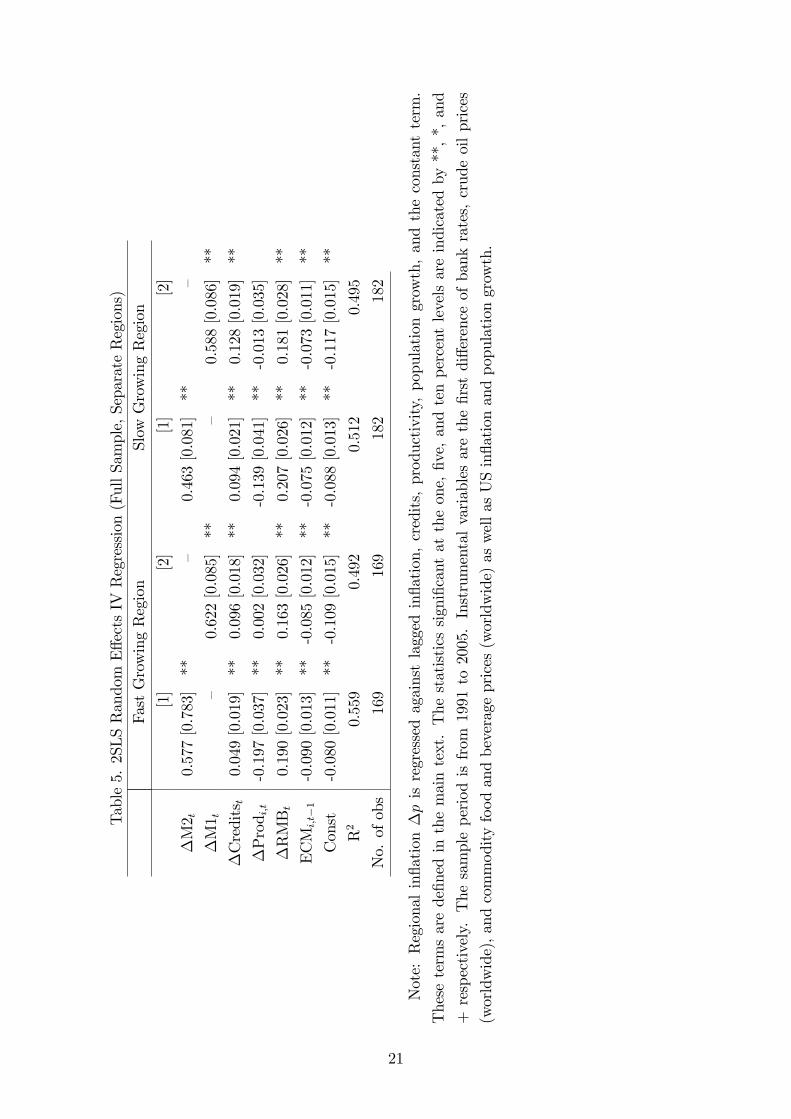
Table5.2SLSRandomE¤ectsIVRegression(FullSample,SeparateRegions)

FastGrowingRegion

SlowGrowingRegion

[1]

[2]

[1]

[2]

�M2 t

0.577[0.783]**

�0.463[0.081]**

�

�M1 t

�0.622[0.085]**

�0.588[0.086]**

�Creditst

0.049[0.019]**

0.096[0.018]**

0.094[0.021]**

0.128[0.019]**

�Prod i;t

-0.197[0.037]**

0.002[0.032]

-0.139[0.041]**

-0.013[0.035]

�RMBt

0.190[0.023]**

0.163[0.026]**

0.207[0.026]**

0.181[0.028]**

ECMi;t�1

-0.090[0.013]**

-0.085[0.012]**

-0.075[0.012]**

-0.073[0.011]**

Const

-0.080[0.011]**

-0.109[0.015]**

-0.088[0.013]**

-0.117[0.015]**

R2

0.559

0.492

0.512

0.495

No.ofobs

169

169

182

182

Note:Regionalin�ation�pisregressedagainstlaggedin�ation,credits,productivity,populationgrowth,andtheconstantterm.

Thesetermsarede�nedinthemaintext.Thestatisticssigni�cantattheone,�ve,andtenpercentlevelsareindicatedby**,*,and

+respectively.Thesampleperiodisfrom

1991to2005.Instrumentalvariablesarethe�rstdi¤erenceofbankrates,crudeoilprices

(worldwide),andcommodityfoodandbeverageprices(worldwide)aswellasUSin�ationandpopulationgrowth.

21

22

Figures Figure 1. Country-Level GDP Growth And Inflation

Data source: The WEO database of the IMF. The GDP growth rate (based on national currency) is the author’s calculation. The CPI is Chinese inflation based on data from the National Bureau of Statistics of China.

-15-10-505

10152025303540

CPI World inflation GDP growth

23

Figure 2. Chinese Exchange Rate vis-à-vis US Dollar.

Source: IMF’s International Financial Statistics

Figure 3. Chinese Retail Price and Consumer Price Indices

Source: National Bureau of Statistics of China

0123456789

1019

8119

8219

8319

8419

8519

8619

8719

8819

8919

9019

9119

9219

9319

9419

9519

9619

9719

9819

9920

0020

0120

0220

0320

0420

0520

06

-10-8-6-4-202468

10

RPI CPI