Giuliano, Paola; Nunn, Nathan

Working Paper

Understanding Cultural Persistence and Change

IZA Discussion Papers, No. 10930

Provided in Cooperation with:IZA – Institute of Labor Economics

Suggested Citation: Giuliano, Paola; Nunn, Nathan (2017) : Understanding Cultural Persistenceand Change, IZA Discussion Papers, No. 10930, Institute of Labor Economics (IZA), Bonn

This Version is available at:http://hdl.handle.net/10419/170914

Standard-Nutzungsbedingungen:

Die Dokumente auf EconStor dürfen zu eigenen wissenschaftlichenZwecken und zum Privatgebrauch gespeichert und kopiert werden.

Sie dürfen die Dokumente nicht für öffentliche oder kommerzielleZwecke vervielfältigen, öffentlich ausstellen, öffentlich zugänglichmachen, vertreiben oder anderweitig nutzen.

Sofern die Verfasser die Dokumente unter Open-Content-Lizenzen(insbesondere CC-Lizenzen) zur Verfügung gestellt haben sollten,gelten abweichend von diesen Nutzungsbedingungen die in der dortgenannten Lizenz gewährten Nutzungsrechte.

Terms of use:

Documents in EconStor may be saved and copied for yourpersonal and scholarly purposes.

You are not to copy documents for public or commercialpurposes, to exhibit the documents publicly, to make thempublicly available on the internet, or to distribute or otherwiseuse the documents in public.

If the documents have been made available under an OpenContent Licence (especially Creative Commons Licences), youmay exercise further usage rights as specified in the indicatedlicence.

Discussion PaPer series

IZA DP No. 10930

Paola GiulianoNathan Nunn

Understanding Cultural Persistence and Change

july 2017

Any opinions expressed in this paper are those of the author(s) and not those of IZA. Research published in this series may include views on policy, but IZA takes no institutional policy positions. The IZA research network is committed to the IZA Guiding Principles of Research Integrity.The IZA Institute of Labor Economics is an independent economic research institute that conducts research in labor economics and offers evidence-based policy advice on labor market issues. Supported by the Deutsche Post Foundation, IZA runs the world’s largest network of economists, whose research aims to provide answers to the global labor market challenges of our time. Our key objective is to build bridges between academic research, policymakers and society.IZA Discussion Papers often represent preliminary work and are circulated to encourage discussion. Citation of such a paper should account for its provisional character. A revised version may be available directly from the author.

Schaumburg-Lippe-Straße 5–953113 Bonn, Germany

Phone: +49-228-3894-0Email: publications@iza.org www.iza.org

IZA – Institute of Labor Economics

Discussion PaPer series

IZA DP No. 10930

Understanding Cultural Persistence and Change

july 2017

Paola GiulianoUCLA Anderson School of Management, NBER, CEPR and IZA

Nathan NunnHarvard University, NBER and BREAD

AbstrAct

july 2017IZA DP No. 10930

Understanding Cultural Persistence and Change*

When does culture persist and when does it change? We examine a determinant that

has been put forth in the anthropology literature: the variability of the environment from

one generation to the next. A prediction, which emerges from a class of existing models

from evolutionary anthropology, is that following the customs of the previous generation

is relatively more beneficial in stable environments where the culture that has evolved up

to the previous generation is more likely to be relevant for the subsequent generation. We

test this hypothesis by measuring the variability of average temperature across 20-year

generations from 500–1900. Looking across countries, ethnic groups, and the descendants

of immigrants, we find that populations with ancestors who lived in environments with

more stability from one generation to the next place a greater importance in maintaining

tradition today. These populations also exhibit more persistence in their traditions over

time.

JEL Classification: N10, Q54

Keywords: cultural persistence, cultural change, tradition

Corresponding author:Paola GiulianoAnderson School of ManagementUniversity of California, Los AngelesLos Angeles, CA 90095USA

E-mail: paola.giuliano@anderson.ucla.edu

* For helpful feedback and comments, the authors thank Ran Abramitzky, Robert Boyd, Jared Diamond, Ruben Durante, Oded Galor, Joseph Henrich, Saumitra Jha, Richard McElreath, Stelios Michalopoulos, Krishna Pendakur, James Robinson, and Paul Smaldino, as well as seminar participants at various seminars and conferences. For help with data, we thank Donna Feir and Jonathan Schulz. We thank Eva Ng and Mohammad Ahmad for excellent research assistance.

1. Introduction

Increasingly, we are coming to understand the role of culture and its importance for economic

development (e.g., Nunn, 2012, Spolaore and Wacziarg, 2013). A number of studies have docu-

mented the persistence of cultural traits over very long periods (e.g., Voigtlaender and Voth, 2012).

Strong cultural persistence that lasts for generations has been documented among migrants and

their descendants (e.g., Fischer, 1989, Fernandez, 2007, Giuliano, 2007, Fernandez and Fogli, 2009,

Algan and Cahuc, 2010). We also have accumulating evidence that vertically transmitted traits,

such as culture or a common history, are important determinants of comparative development

today (Spolaore and Wacziarg, 2009, Comin, Easterly and Gong, 2010, Chanda and Putterman,

2014). Along similar lines, numerous studies show how deep historical factors can shape persis-

tent cultural traits (Giuliano and Nunn, 2013, Alesina, Giuliano and Nunn, 2013, Talhelm, Zhang,

Oishi, Shimin, Duan, Lan and Kitayama, 2014, Becker, Boeckh, Hainz and Woessmann, 2016,

Buggle and Durante, 2016, Guiso, Sapienza and Zingales, 2016).

On the other hand, there are also numerous examples of a lack of cultural persistence; namely,

episodes of significant cultural change. A well-studied episode of cultural change is the Protestant

Reformation in Europe (e.g., Becker and Woessmann, 2008, 2009, Cantoni, 2012, 2014). Another

example, though on a smaller scale, is the Puritan colony established on Providence Island,

off of the coast of Nicaragua, in the early seventeenth century (Kupperman, 1995). Unlike

the Puritan colony established in Massachusetts, this colony experienced a significant cultural

change. Abandoning their traditional values, the Puritans began large-scale use of slaves and

engaged in privateering. Margaret Mead’s (1956) ethnography of the Manus documents how, in a

single generation, this society completely changed its culture, abandoning the previous practices

of living in stilt houses on the sea to living on land, wearing European clothes, and adopting

European institutional structures in the villages. Firth (1959) documents similar dramatic cultural

changes that occurred within one generation among the Polynesian community of Tikopia.1

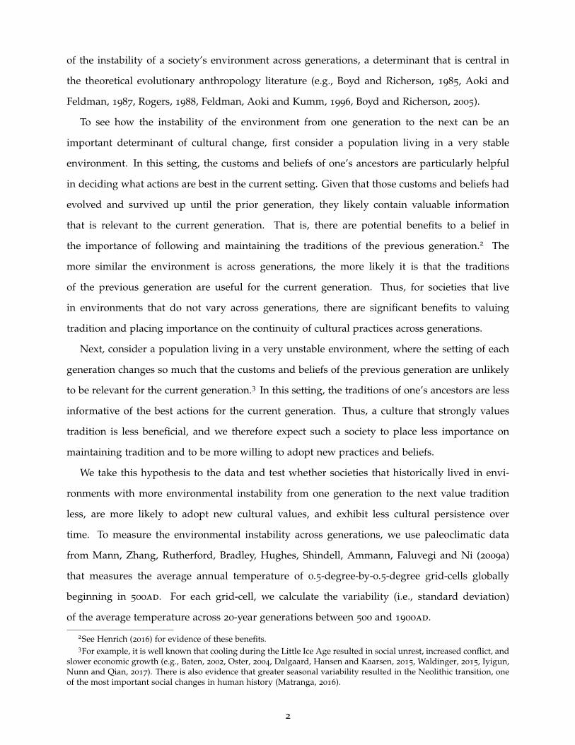
Given that we have numerous examples of cultural persistence and numerous examples of

cultural change, a question naturally arises: when does culture change and when does it persist?

In particular, what determines a society’s willingness to adopt new customs and beliefs rather

than hold on to traditions? We consider this question here. Specifically, we test for the importance

1Also related are studies that find evidence of a lack of economic persistence and even reversals (see for exampleAcemoglu, Johnson and Robinson, 2002, Olsson and Paik, 2012).

1

of the instability of a society’s environment across generations, a determinant that is central in

the theoretical evolutionary anthropology literature (e.g., Boyd and Richerson, 1985, Aoki and

Feldman, 1987, Rogers, 1988, Feldman, Aoki and Kumm, 1996, Boyd and Richerson, 2005).

To see how the instability of the environment from one generation to the next can be an

important determinant of cultural change, first consider a population living in a very stable

environment. In this setting, the customs and beliefs of one’s ancestors are particularly helpful

in deciding what actions are best in the current setting. Given that those customs and beliefs had

evolved and survived up until the prior generation, they likely contain valuable information

that is relevant to the current generation. That is, there are potential benefits to a belief in

the importance of following and maintaining the traditions of the previous generation.2 The

more similar the environment is across generations, the more likely it is that the traditions

of the previous generation are useful for the current generation. Thus, for societies that live

in environments that do not vary across generations, there are significant benefits to valuing

tradition and placing importance on the continuity of cultural practices across generations.

Next, consider a population living in a very unstable environment, where the setting of each

generation changes so much that the customs and beliefs of the previous generation are unlikely

to be relevant for the current generation.3 In this setting, the traditions of one’s ancestors are less

informative of the best actions for the current generation. Thus, a culture that strongly values

tradition is less beneficial, and we therefore expect such a society to place less importance on

maintaining tradition and to be more willing to adopt new practices and beliefs.

We take this hypothesis to the data and test whether societies that historically lived in envi-

ronments with more environmental instability from one generation to the next value tradition

less, are more likely to adopt new cultural values, and exhibit less cultural persistence over

time. To measure the environmental instability across generations, we use paleoclimatic data

from Mann, Zhang, Rutherford, Bradley, Hughes, Shindell, Ammann, Faluvegi and Ni (2009a)

that measures the average annual temperature of 0.5-degree-by-0.5-degree grid-cells globally

beginning in 500ad. For each grid-cell, we calculate the variability (i.e., standard deviation)

of the average temperature across 20-year generations between 500 and 1900ad.

2See Henrich (2016) for evidence of these benefits.3For example, it is well known that cooling during the Little Ice Age resulted in social unrest, increased conflict, and

slower economic growth (e.g., Baten, 2002, Oster, 2004, Dalgaard, Hansen and Kaarsen, 2015, Waldinger, 2015, Iyigun,Nunn and Qian, 2017). There is also evidence that greater seasonal variability resulted in the Neolithic transition, oneof the most important social changes in human history (Matranga, 2016).

2

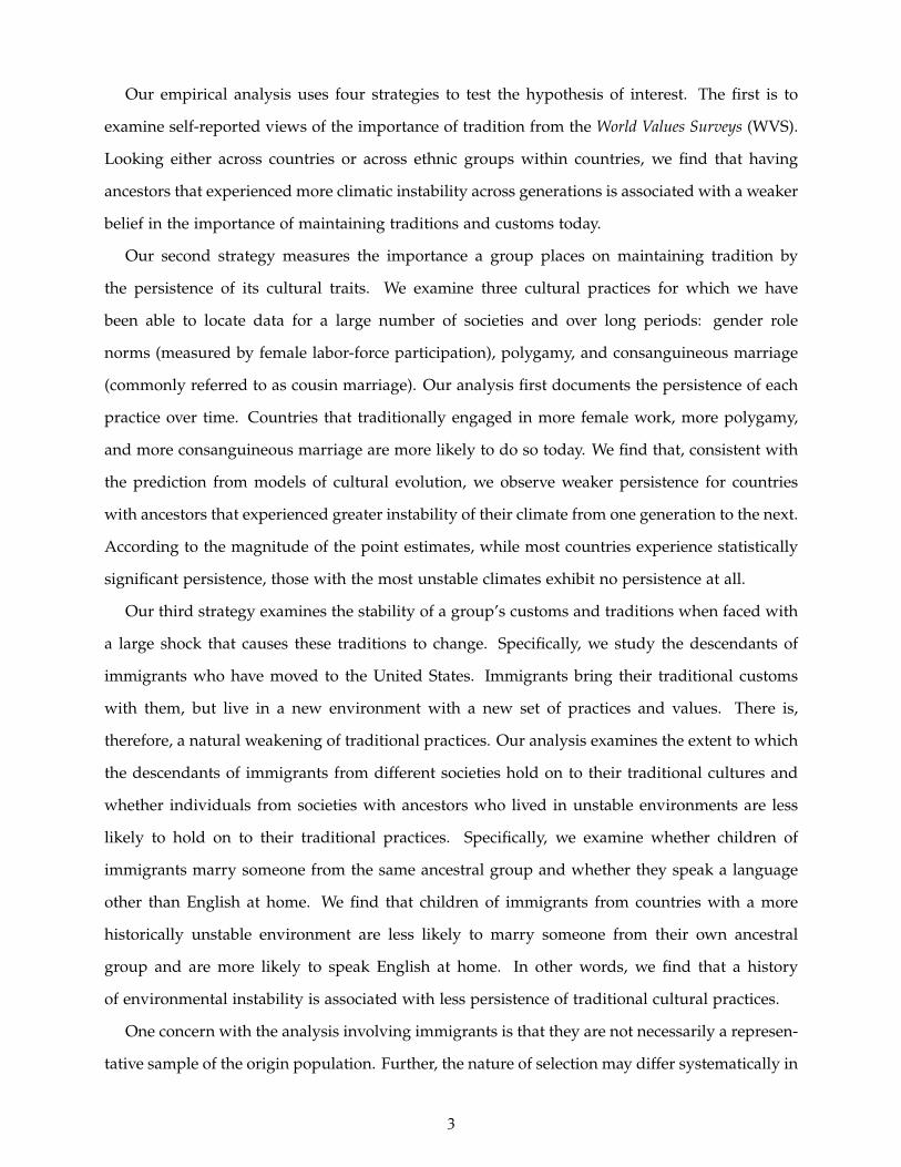
Our empirical analysis uses four strategies to test the hypothesis of interest. The first is to

examine self-reported views of the importance of tradition from the World Values Surveys (WVS).

Looking either across countries or across ethnic groups within countries, we find that having

ancestors that experienced more climatic instability across generations is associated with a weaker

belief in the importance of maintaining traditions and customs today.

Our second strategy measures the importance a group places on maintaining tradition by

the persistence of its cultural traits. We examine three cultural practices for which we have

been able to locate data for a large number of societies and over long periods: gender role

norms (measured by female labor-force participation), polygamy, and consanguineous marriage

(commonly referred to as cousin marriage). Our analysis first documents the persistence of each

practice over time. Countries that traditionally engaged in more female work, more polygamy,

and more consanguineous marriage are more likely to do so today. We find that, consistent with

the prediction from models of cultural evolution, we observe weaker persistence for countries

with ancestors that experienced greater instability of their climate from one generation to the next.

According to the magnitude of the point estimates, while most countries experience statistically

significant persistence, those with the most unstable climates exhibit no persistence at all.

Our third strategy examines the stability of a group’s customs and traditions when faced with

a large shock that causes these traditions to change. Specifically, we study the descendants of

immigrants who have moved to the United States. Immigrants bring their traditional customs

with them, but live in a new environment with a new set of practices and values. There is,

therefore, a natural weakening of traditional practices. Our analysis examines the extent to which

the descendants of immigrants from different societies hold on to their traditional cultures and

whether individuals from societies with ancestors who lived in unstable environments are less

likely to hold on to their traditional practices. Specifically, we examine whether children of

immigrants marry someone from the same ancestral group and whether they speak a language

other than English at home. We find that children of immigrants from countries with a more

historically unstable environment are less likely to marry someone from their own ancestral

group and are more likely to speak English at home. In other words, we find that a history

of environmental instability is associated with less persistence of traditional cultural practices.

One concern with the analysis involving immigrants is that they are not necessarily a represen-

tative sample of the origin population. Further, the nature of selection may differ systematically in

3

a manner that is correlated with the cross-generational climatic instability of the origin country.

Given these concerns, our fourth strategy examines non-immigrant populations that are faced

with pressure to change their traditions and customs: Indigenous populations of the United

States and Canada. Like immigrants, Indigenous populations are minority groups whose cultural

traditions differ from those of the majority population. However, unlike immigrants, they are not

a small subset of a larger population that has been selected by the immigration process. Our

analysis examines the relationship between the cross-generational climatic instability of the land

historically inhabited by Indigenous groups and the extent to which they are able to speak their

traditional language today. We find that, as with the descendants of immigrants, Indigenous

populations with a history of greater environmental instability are less likely to speak their

traditional language. They appear to have been more likely to abandon this cultural tradition

and to adopt English as the language spoken at home.

Overall, each of our four strategies yields the same conclusion: tradition is less important and

culture less persistent among populations with ancestors who lived in environments that changed

more from generation to generation.

Our results contribute to a deeper understanding of cultural persistence and change. Two

previous studies use lab-based methods to test the prediction of the relationship between the

stability of the environment and cultural persistence that arises from models of cultural evolution

(McElreath, Lubell, Richerson, Waring, Baum, Edstein, Efferson and Paciotti, 2005, Toelch, van

Delft, Bruce, Donders, Meeus and Reader, 2009).4 McElreath et al. (2005) examine the behavior

of 30–40 student participants (depending on the experiment), who played the role of farmers,

choosing which of two crops to plant over twenty consecutive planting seasons. In one of the

modules of the experiment, students could choose to learn the planting choices of participants

from the previous season before making their decision. The authors found that reliance on social

learning (or tradition) is lower when there is less stability in the payoffs to planting each crop.

A subsequent experiment implemented by Toelch et al. (2009) with 62 undergraduate students

yielded the same finding. In that experiment, participants attempted to find a reward within a

virtual maze. There were three treatment groups that varied in the probability that the location of

the reward would change after each of 100 rounds. The authors found that more social learning

4Prior to these studies, Galef and Whiskin (2004) had used rats to test for a relationship between the stability of theenvironment and social learning. Consistent with the models, they found that social learning was stronger when theenvironment was more stable.

4

occurred (i.e., behavior was more influenced by the actions and payoffs of others) when the

environment was less variable.

A number of studies in economics provide important insights into the process of cultural

change. Fouka (2015) studies the effects of language restrictions against German schools in the

United States in the early twentieth century. She finds that these restrictions actually strengthened

the value placed on German culture and identity, and strengthened its transmission over genera-

tions. Specifically, she finds that the restrictions increased the rate of within-group marriage and

the choice of distinctively German names for children. Along similar lines, Abramitzky, Boustan

and Eriksson (2016) examine the naming practices of immigrants who arrived in the United States

at the end of the Age of Mass Migration. The authors use the foreignness of child names to trace

out the extent of immigrants’ cultural assimilation over time. They find that parents tend to

choose less-foreign names the longer they are in the United States. They also find that the speed

of assimilation varies significantly across origin-countries. Our study can be seen as testing one

hypothesis that explains this variation in cultural assimilation.

Giavazzi, Petkov and Schiantarelli (2014) study the complementary question of which types

of cultural traits tend to persist and which types tend not to. The authors examine the children

of immigrants to Europe and the United States and document that certain cultural traits exhibit

strong persistence – namely, religious values and political orientation – while others – such as,

attitudes towards cooperation, independence, and women’s work – do not. Voigtlaender and

Voth (2012) show that the persistence of anti-Semitic attitudes in Germany over a 600-year period

was weaker in towns that were more economically dynamic or were more open to external trade.

Our findings are consistent with this prior evidence. One can interpret German towns with

faster economic growth and greater openness to external trade as being inherently less stable and

therefore we expect cultural persistence to be weaker.

On the theoretical front, Greif and Tadelis (2010) examine the persistence of cultural values in

a setting with an authority, such as a state or church, that is attempting to change the population’s

cultural values. The authors allow for the population to engage in actions that differ from their

true values and to pass on values to their children that differ from those reflected by their actions.

They model how the persistence of cultural values differs depending on the extent to which

the authority can detect and punish hidden beliefs. They also consider the possibility of direct

socialization by the state; for example, through centralized state schooling. Iyigun and Rubin

5

(2017) consider the related question of when societies adopt new institutions and when they hold

on to traditional institutions, even if those are less efficient. In their setting, uncertainty associated

with the new institutions causes people to place a higher value on traditional practices, which

decreases the likelihood of institutional innovation. Doepke and Zilibotti (2017) study the specific

strategies – permissive, authoritarian, and authoritative – that parents use to induce the desired

outcomes for their children. In their model, the strategy chosen by parents has implications for

the persistence of behavior across generations.

Our findings also provide empirical validation of a class of models from evolutionary an-

thropology that provide a foundation for the assumptions made in the models used in cultural

economics (e.g., Bisin and Verdier, 2000, 2001, Hauk and Saez-Marti, 2002, Francois and Zabojnik,

2005, Tabellini, 2008, Greif and Tadelis, 2010, Bisin and Verdier, 2017, Doepke and Zilibotti, 2017).

Within this class of evolutionary models, under general circumstances, some proportion of the

population finds it optimal to rely on social learning – that is, culture – when making decisions.

This result provides a justification for the assumption in models of cultural evolution that parents

choose to – and are able to – influence the preferences of their children.

The next section of the paper describes the hypothesis and its mechanisms using a simple

model. The model shows, in the simplest possible terms, how a stable environment tends to

favor a cultural belief in the importance of tradition and therefore generates cultural persistence.

In Section 3, we describe the data used in the analysis. In Sections 4–7, we describe our empirical

tests and report the results. Section 8 concludes.

2. The model

We now present a simple model that highlights the intuition of how variability of the environment

between generations can affect the extent to which individuals value the importance of tradition.

The insight that emerges from the model is that it is relatively less beneficial to value (and follow)

the traditions of the previous generation when the environment is less stable. Intuitively, this

is because the traditions and actions that have evolved up to the previous generation are less

likely to be suitable for the environment of the current generation. This insight emerges from a

wide range of models of cultural evolution in the evolutionary anthropology literature e.g., Boyd

and Richerson (1985, chpt. 4), Rogers (1988), and Boyd and Richerson (1988). The model that we

present here reproduces the basic logic of the model from Rogers (1988).

6

Players

The players of the game consist of a continuum of members of a society. Each period, a new

generation is born and the previous generation dies.

Actions

In each period (generation), individuals choose one of two possible actions, which we denote 0

and 1. Which of the two actions yields a higher payoff depends on the state of the world, which

can be either 0 or 1. The payoffs to each action in each state is given below, where π > 0 and

b > 0. When the state is 0, action 0 yields a higher payoff and when the state is 1, action 1 yields

a higher payoff.

Environment0 1

0 π+ b π− bAction

1 π− b π+ b

In each period, there is some probability ∆ ∈ [0,1] of a shock. When a shock is experienced,

there is a new draw and it is equally likely that the draw results in the new environment being

state 0 or state 1. The state of the world is unknown to the players. However, as we explain below,

it is possible to engage in learning (at a cost) to determine the state of the world.

Player Types

There are two possible types of players, each with a different method of choosing an action.5 We

describe the two types below.

1. Traditionalists (T) value tradition and place strong importance on the actions (culture) of

the previous generation. They choose their action by following the action of a randomly

chosen person from the previous generation.

2. Non-Traditionalists (NT) do not value tradition and ignore the actions (culture) of the

previous generation. Instead, they invest an amount 0 to learn with certainty the optimal

5Rogers’ (1988) original interpretation was that a player’s type was hardwired, being biologically determined, andtherefore subject to evolutionary forces.

7

action for the current period. It is assumed that the cost of learning, though positive, is

modest and satisfies: c ∈ (0, b).6

Let p ∈ [0, 1] denote the proportion of traditionalists in the population. Thus, p is a measure

of the overall strength of tradition in the society: the proportion of the population that values

tradition and follows the actions of the previous generation, rather than ignoring tradition and

acting based on one’s belief about what action is best.

Payoffs

First, consider the expected payoff of a non-traditionalist. In each generation, they learn and

choose the optimal action and receive π + b. However, they also bear the cost of learning, which

is equal to c. Thus, the payoff to a non-traditionalist is:

ΠNT = π+ b− c

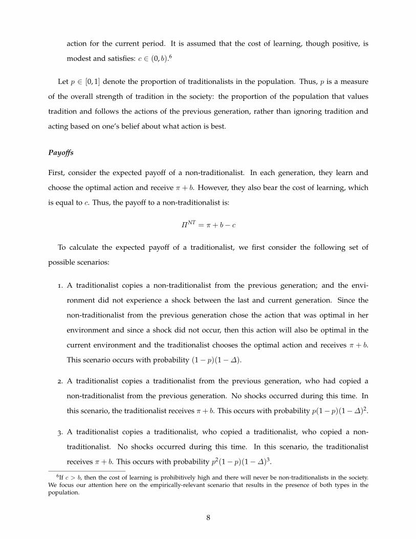
To calculate the expected payoff of a traditionalist, we first consider the following set of

possible scenarios:

1. A traditionalist copies a non-traditionalist from the previous generation; and the envi-

ronment did not experience a shock between the last and current generation. Since the

non-traditionalist from the previous generation chose the action that was optimal in her

environment and since a shock did not occur, then this action will also be optimal in the

current environment and the traditionalist chooses the optimal action and receives π + b.

This scenario occurs with probability (1− p)(1−∆).

2. A traditionalist copies a traditionalist from the previous generation, who had copied a

non-traditionalist from the previous generation. No shocks occurred during this time. In

this scenario, the traditionalist receives π+ b. This occurs with probability p(1− p)(1−∆)2.

3. A traditionalist copies a traditionalist, who copied a traditionalist, who copied a non-

traditionalist. No shocks occurred during this time. In this scenario, the traditionalist

receives π+ b. This occurs with probability p2(1− p)(1−∆)3.

6If c > b, then the cost of learning is prohibitively high and there will never be non-traditionalists in the society.We focus our attention here on the empirically-relevant scenario that results in the presence of both types in thepopulation.

8

4. Copies a traditionalist, who copied a traditionalist, who copied a traditionalist, who copied

a non-traditionalist. No shocks occurred during this time. In this scenario, the traditionalist

receives π+ b. This occurs with probability p3(1− p)(1−∆)4.

5. Etc, etc.

One can continue this sequence until infinity. Summing the infinite sequence of probabilities

gives: ∑∞t=1 p

t−1(1− p)(1−∆)t.

Conversely, with probability 1− ∑∞t=1 p

t−1(1− p)(1−∆)t, a traditionalist does not obtain the

correct action with certainty. In these cases, at least one shock to the environment has occurred.

Recall that after a shock there is an equal probability of being in either state. Thus, a traditionalist

still has a 50% chance of choosing the correct action for the state and receiving π + b and a 50%

chance of choosing the wrong action and receiving π − b, and the expected payoff in these cases

is π.

Putting this all together, the expected payoff to a traditionalist is given by:

ΠT = [∞

∑t=1

pt−1(1− p)(1−∆)t](π+ b) + [1−∞

∑t=1

pt−1(1− p)(1−∆)t][12(π+ b) +

12(π− b)]

= π+ b(1− p)(1−∆)∞

∑t=1

pt−1(1−∆)t−1

= π+b(1− p)(1−∆)

1− p(1−∆)

The payoffs to both traditionalists and non-traditionalists over all potential values of p ∈ [0,1]

(the proportion of traditionalists in the society) are shown in Figure 1a. As shown, the expected

payoff of a traditionalist, ΠT , is decreasing in p, the proportion of traditionalists in the society.

Intuitively, this is because as the fraction of traditionalists increases, it is less likely that a

traditionalist will copy a non-traditionalist who is more likely to have chosen the correct action.

At the extreme, where everyone in the population is a traditionalist (p = 1), each traditionalist

copies another traditionalist and the expected payoff is π. With 50% probability, one receives π+ b

and with 50% probability, one receives π− b.

At the other extreme, where everyone is a non-traditionalist (p = 0), a (mutant) traditionalist

would copy the correct action from someone in the previous generation as long as there was

not a shock to the environment between the two generations. Thus, with probability 1−∆, a

traditionalist’s payoff is π + b. If, on the other hand, the environment did change, which occurs

9

with probability ∆, then there is an equal probability that the environment is in either state

and the expected payoff is π. Therefore, the expected payoff to a traditionalist when p = 0 is:

∆π+ (1−∆)(π+ b) = π+ b(1−∆).

Figure 1b illustrates how the payoffs of traditionalists and non-traditionalists change as the

environment becomes less stable; that is, as ∆ increases. More instability causes the payoffs to

the traditionalists to decline and the payoff curve rotates downwards. By contrast, the payoffs to

the non-traditionalists are unaffected. Therefore, an increase in cross-generational environmental

instability results in a decline in the equilibrium proportion of traditionalists in the society.

Equilibrium and comparative statics

From Figures 1a and 1b, it is clear that under fairly general conditions (∆ < c/b), the equilibrium

has both traditionalists and non-traditionalists present in the society. It is only when instability,

∆, is sufficiently great (such that ∆ > c/b), that the society has no traditionalists (p = 0).

Thus, the model predicts that under fairly general conditions, we should observe the existence

of traditionalists (and of cultural transmission). This is due to the value of relying on tradition,

which allows for a quick and easy decision-making heuristic: simply rely on the traditional

practices of the previous generation. The evidence suggests that this is the empirically relevant

scenario. There are many real-world examples of functional traits evolving and being followed

despite the population not knowing their benefits. One of the best known is alkali processing of

maize, which is the traditional method of preparing maize in Latin America. During the process,

dried maize is boiled in a mixture of water and either limestone or ash, before being mashed into

a dough called ‘masa’. Although it was unknown at the time, putting limestone or ash in the

water before boiling prevents pellagra, a disease resulting from niacin deficiency, which occurs

in diets that consist primarily of maize. This is because the alkaline solution that results from

the inclusion of limestone or ash increases the body’s absorption of niacin (Katz, Hediger and

Valleroy, 1974).7

In equilibria with both types present, their payoffs must be equal. Using this condition, and

solving for the equilibrium proportion of traditionalists in the economy, gives: p∗ = c−∆bc(1−∆)

. The

7For other examples and additional evidence along these lines, see Henrich (2015).

10

π+b(1-Δ)

π+b-c∏NT=π+b-c

∏T=π+b(1-p)(1-Δ)/[1-p(1-Δ)]

10

Proportionoftraditionalistsinthepopulation,p

Long-Run

Payoffs

p*

π

(a) Payoffs to traditionalists and non-traditionalists as a function of the proportion of traditionalists in thesociety.

π+b(1-Δ)

π+b-c∏NT=π+b-c

∏T=π+b(1-p)(1-Δ)/[1-p(1-Δ)]

10

Proportionoftraditionalistsinthepopulation,p

Long-Run

Payoffs

p*

π

π+b(1-Δ´)

p´*

(b) Effects of an increase in the instability of the environment.

Figure 1: The equilibrium proportion of traditionalists (T) and non-traditionalists (NT) in themodel.

11

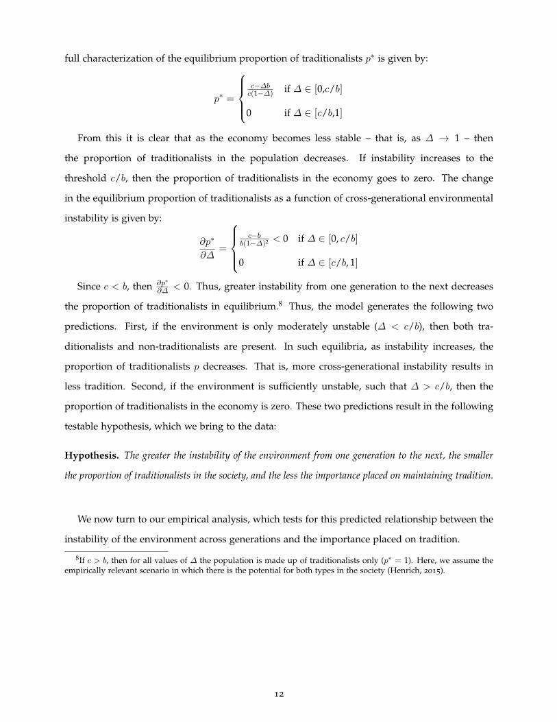
full characterization of the equilibrium proportion of traditionalists p∗ is given by:

p∗ =

c−∆bc(1−∆)

if ∆ ∈ [0,c/b]

0 if ∆ ∈ [c/b,1]

From this it is clear that as the economy becomes less stable – that is, as ∆ → 1 – then

the proportion of traditionalists in the population decreases. If instability increases to the

threshold c/b, then the proportion of traditionalists in the economy goes to zero. The change

in the equilibrium proportion of traditionalists as a function of cross-generational environmental

instability is given by:

∂p∗

∂∆=

c−b

b(1−∆)2 < 0 if ∆ ∈ [0, c/b]

0 if ∆ ∈ [c/b, 1]

Since c < b, then ∂p∗

∂∆ < 0. Thus, greater instability from one generation to the next decreases

the proportion of traditionalists in equilibrium.8 Thus, the model generates the following two

predictions. First, if the environment is only moderately unstable (∆ < c/b), then both tra-

ditionalists and non-traditionalists are present. In such equilibria, as instability increases, the

proportion of traditionalists p decreases. That is, more cross-generational instability results in

less tradition. Second, if the environment is sufficiently unstable, such that ∆ > c/b, then the

proportion of traditionalists in the economy is zero. These two predictions result in the following

testable hypothesis, which we bring to the data:

Hypothesis. The greater the instability of the environment from one generation to the next, the smaller

the proportion of traditionalists in the society, and the less the importance placed on maintaining tradition.

We now turn to our empirical analysis, which tests for this predicted relationship between the

instability of the environment across generations and the importance placed on tradition.

8If c > b, then for all values of ∆ the population is made up of traditionalists only (p∗ = 1). Here, we assume theempirically relevant scenario in which there is the potential for both types in the society (Henrich, 2015).

12

3. Data: Sources and their construction

A. Motivating the measure of environmental instability

When bringing the model and its predictions to the data, the primary decision is how to measure

the variability of the environment, ∆. While there are many aspects of a society’s environment

that one could measure, we focus on a measure that is exogenous (that is, unaffected by human

actions) and is likely to affect the optimal decisions of daily life.

The measure of the environment that we use is temperature. As we explain in more detail

below, we measure the historical variability of temperature across 20-year generations from

500 to 1900ad. During this time, temperature was exogenous since it was not affected in any

significant manner by human actions. There is also mounting evidence that weather and climate

have important effects on societies. For example, a number of studies now show that cooling

during the Little Ice Age resulted in worse health outcomes, social unrest, increased conflict,

decreased productivity, and slower economic growth (e.g., Baten, 2002, Oster, 2004, Waldinger,

2015, Dalgaard et al., 2015, Iyigun et al., 2017). There is evidence that increased seasonal variability

in certain locations resulted in the Neolithic transition, one of the most important social changes in

human history (Matranga, 2016). Durante (2010) and Buggle and Durante (2016) find that, within

Europe, greater year-to-year variability in temperature and precipitation during the growing

season is associated with greater trust. Also related are recent findings that rarely occurring

environmental shocks can affect cultural beliefs, such as religiosity (Chaney, 2013, Bentzen, 2015,

Belloc, Drago and Galbiati, 2016). There is growing evidence from contemporary data that

changes in temperature have important effects, including effects on civil conflict (Burke, Miguel,

Satyanath, Dykema and Lobell, 2009), violent crime (Hsiang, Burke and Miguel, 2013), economic

output (Burke, Hsiang and Miguel, 2015, Dell, Jones and Olken, 2012), economic growth (Dell et

al., 2012), agricultural output (Dell et al., 2012), and political instability (Dell et al., 2012).

Although we cannot observe the relationship between the environment and the optimal action

(or the payoffs to different actions), we have mounting evidence that changes in the environment

affect important equilibrium outcomes like conflict, cooperation, trust, trade, and economic pros-

perity. This provides evidence that the environment is an important determinant of the optimal

actions for a society at a given time. The evidence suggests that temperature has important effects

on the returns to cooperation, to trade, and to conflict. Thus, it plausibly affects the optimal

13

level of cooperation, entrepreneurship, conflict, and so on. In addition, it directly and more

mechanically affects the optimal decisions in agriculture, the optimal intensity of agriculture,

what crops should be planted and when, and what agricultural implements to use. Thus, our

constructed variable then measures how average temperature – and therefore the optimal actions

in a society – change from one generation to the next.

An alternative strategy would be to look at changes in more proximate variables, like income,

population density, or innovation.9 While such an exercise would be informative, these deter-

minants are potentially endogenous. In addition, to the extent that cross-generational climatic

instability has an effect on these more proximate factors, the reduced-form relationship between

climatic instability and the importance of tradition already captures effects working through these

mechanisms.

B. Measuring the instability of the environment across previous generations

We use data collected by Mann et al. (2009a) covering the entire world. The original dataset

includes gridded average temperatures (0.5-degree-by-0.5-degree grid-cells) annually from 500 to

1900. Mann et al. use a climate field reconstruction approach to reconstruct global patterns

of surface temperature for a long historical period. The construction uses proxy data with

global coverage that comprises 1,036 tree ring series, 32 ice core series, 15 marine coral series, 19

documentary series, 14 speleothem series, 19 lacustrine sediment series, and 3 marine sediment

series (Mann, Zhang, Rutherford, Bradley, Hughes, Shindell, Ammann, Faluvegi and Ni, 2009b).

Let xg be the average temperature during a given generation g. Generations are 20 years in

length and, thus, there are 70 generations from 500–1900. Our measure of interest is the standard

deviation of the average temperature across generations:

[1Ng

70∑g=1

(xg − x)2

]1/2

.

The average variability by grid-cell is shown in Figure 2, where yellow (a lighter shade) indi-

cates less variability and brown (a darker shade) greater variability. Although there is variation

between nearby cells, there are also some broad patterns. For example, cells that are further from

the equator tend to have greater variability.

Our analysis examines the relationship between measures of the importance of tradition in

the contemporary period and the instability of the climate of an individual’s ancestors. Thus, an

9Voigtlaender and Voth (2012), for example, show that the persistence of anti-Semitic attitudes in Germany over a600-year period was weaker in towns that were more economically dynamic or more open to external trade.

14

Clim

atic

Varia

bility

No D

ata

0.001

- 0.09

70.0

98 - 0

.129

0.130

- 0.15

5

0.156

- 0.18

10.1

82 - 0

.211

0.212

- 0.24

6

0.247

- 0.29

20.2

93 - 0

.376

0.377

- 0.90

9

Ü0

1,700

850

Miles

Figu

re2:

Gri

d-ce

ll-le

velh

isto

rica

ltem

pera

ture

vari

abili

tyac

ross

gene

rati

ons

from

500–1

900.

15

important part of the analysis is to correctly identify the historical locations of an individual’s

ancestors. One method that we use is to rely on the self-reported ethnicity of a respondent. To

identify an ethnic group’s historical location, we use Murdock’s (1967) Ethnographic Atlas, which

reports the latitude and longitude of the centroid of the traditional location of 1,265 ethnic groups

across the world.

To extend the precision and coverage of the Ethnographic Atlas, we also use two ethnographic

samples that were published in the journal Ethnology in 2004 and 2005. Peoples of Easternmost Eu-

rope was constructed by Bondarenko, Kazankov, Khaltourina and Korotayev (2005) and includes

seventeen ethnic groups from Eastern Europe that are not in the Ethnographic Atlas. Peoples of

Siberia was constructed by Korotayev, Kazankov, Borinskaya and Khaltourina (2004) and includes

ten additional Siberian ethnic groups. We use this extended sample of 1,292 ethnic groups as a

second ethnographic sample for our analysis.

We also use a third (and even larger) sample. In 1957, prior to the construction of the

Ethnographic Atlas, George Peter Murdock constructed the World Ethnographic Sample, which

was published in Ethnology (see Murdock, 1957). Most of the ethnic groups from the World

Ethnographic Sample later appeared in the Ethnographic Atlas, but seventeen ethnic groups did not.

Those were ethnic groups for which information was more limited; if they had been included in

the Ethnographic Atlas, they would have had a number of variables with missing values. In our

analysis, we also use a third extended sample of 1,309 ethnic groups, which also includes the

World Ethnographic Sample. As we will show, our estimates are very similar irrespective of which

ethnographic sample we use.

For each of the 1,309 ethnic groups in our samples, we know the coordinates of the centroid of

its historical location. These are shown in Figure 3. By identifying the climatic grid-cell for each

location, we have an estimate of the climatic instability across generations that was faced by each

group.

For much of our analysis, we are able to identify the climatic instability faced by an individual’s

ancestors using ethnicity. In these cases, we simply need to match the ethnicities reported in our

dataset with the 1,309 ethnic groups from our ethnographic data, which we do manually.

In other parts of our analysis, we use a person’s country to obtain an estimate of the historical

climatic instability across generations. This requires a measure of the average cross-generational

instability faced by the ancestors of those living in each country today. We construct this using

16

LegendEthnographic AtlasEasternmost EuropeSiberiaWES

.

0 1,400 2,800 Miles

Figure 3: Locations of the centroids of ethnic groups in the Ethnographic Atlas, Peoples of Eastern-most Europe, Peoples of Siberia, and World Ethnographic Sample (WES).

a procedure similar to that used in Alesina et al. (2013). First, we match each of the 1,309 ethnic

groups in our ethnographic samples to one of the 7,000+ languages and dialects in the world

today, as categorized and mapped by the Ethnologue 16. This, combined with 1km by 1km gridded

population data from Landscan, provides us with an estimate of the identity of the ancestors of all

populations in the world at a 1km resolution.10 Through this match of languages to ethnicities, we

create a measure of the estimated instability of the climate between generations of the ancestors

of all individuals living across the globe at a 1 kilometer resolution.11

With the gridded information, we construct average cross-generational climatic instability

measures across all individuals in a country. We use these for those parts of our analysis for

which countries are the unit of observation. The country-level measures are shown in Figure 4.

As with the grid-level variation, places further from the equator tend to show more variability.

In addition, some of the richer countries also appear to have greater variability. Given that these

factors could independently affect our outcomes of interest, in our empirical analysis, we control

for distance from the equator as well as average per-capita income.

Although our empirical strategy accounts for the large migrations that have occurred since

1500, following the Columbian Exchange, there remains the issue of the extent to which ancestral

locations in the ethnographic data are accurate for the period of interest, 500–1900. Other than the

10Alesina et al. (2013) used Ethnologue 15 in their matching procedure, which was the most current version at thetime.

11For the finer details on the construction of the data, see Giuliano and Nunn (2016). For another application of thesame data construction procedure, see Giuliano and Nunn (2013).

17

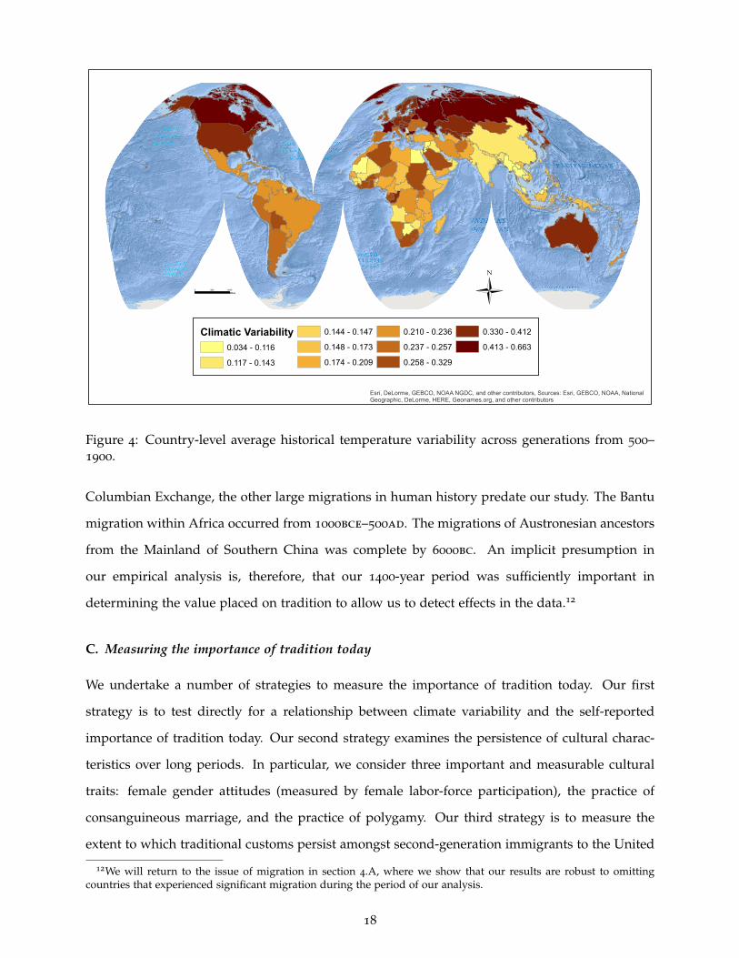
Esri, DeLorme, GEBCO, NOAA NGDC, and other contributors, Sources: Esri, GEBCO, NOAA, NationalGeographic, DeLorme, HERE, Geonames.org, and other contributors

Climatic Variability0.034 - 0.1160.117 - 0.143

0.144 - 0.1470.148 - 0.1730.174 - 0.209

0.210 - 0.2360.237 - 0.2570.258 - 0.329

0.330 - 0.4120.413 - 0.663

Ü0 1,600800Miles

Figure 4: Country-level average historical temperature variability across generations from 500–1900.

Columbian Exchange, the other large migrations in human history predate our study. The Bantu

migration within Africa occurred from 1000bce–500ad. The migrations of Austronesian ancestors

from the Mainland of Southern China was complete by 6000bc. An implicit presumption in

our empirical analysis is, therefore, that our 1400-year period was sufficiently important in

determining the value placed on tradition to allow us to detect effects in the data.12

C. Measuring the importance of tradition today

We undertake a number of strategies to measure the importance of tradition today. Our first

strategy is to test directly for a relationship between climate variability and the self-reported

importance of tradition today. Our second strategy examines the persistence of cultural charac-

teristics over long periods. In particular, we consider three important and measurable cultural

traits: female gender attitudes (measured by female labor-force participation), the practice of

consanguineous marriage, and the practice of polygamy. Our third strategy is to measure the

extent to which traditional customs persist amongst second-generation immigrants to the United

12We will return to the issue of migration in section 4.A, where we show that our results are robust to omittingcountries that experienced significant migration during the period of our analysis.

18

States. Specifically, we examine whether the children of immigrant parents marry someone from

their same origin-group and whether they speak their origin language at home. We interpret both

as revealed measures about the strength of the value placed on maintaining the traditions and

customs of the origin country. Our fourth strategy is to measure the extent to which Indigenous

populations in the United States and Canada continue to speak their native languages.

4. Climatic instability and the importance of tradition: Evidence from self-reports

from the WVS

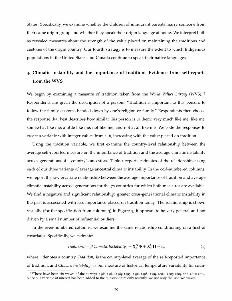
We begin by examining a measure of tradition taken from the World Values Survey (WVS).13

Respondents are given the description of a person: “Tradition is important to this person; to

follow the family customs handed down by one’s religion or family.” Respondents then choose

the response that best describes how similar this person is to them: very much like me; like me;

somewhat like me; a little like me; not like me; and not at all like me. We code the responses to

create a variable with integer values from 1–6, increasing with the value placed on tradition.

Using the tradition variable, we first examine the country-level relationship between the

average self-reported measure on the importance of tradition and the average climatic instability

across generations of a country’s ancestors. Table 1 reports estimates of the relationship, using

each of our three variants of average ancestral climatic instability. In the odd-numbered columns,

we report the raw bivariate relationship between the average importance of tradition and average

climatic instability across generations for the 75 countries for which both measures are available.

We find a negative and significant relationship: greater cross-generational climatic instability in

the past is associated with less importance placed on tradition today. The relationship is shown

visually (for the specification from column 3) in Figure 5; it appears to be very general and not

driven by a small number of influential outliers.

In the even-numbered columns, we examine the same relationship conditioning on a host of

covariates. Specifically, we estimate:

Traditionc = β Climatic Instabilityc + XHc Φ + XCc Π + εc (1)

where c denotes a country, Traditionc is the country-level average of the self-reported importance

of tradition, and Climatic Instabilityc is our measure of historical temperature variability for coun-

13There have been six waves of the survey: 1981-1984, 1989-1993, 1994-1998, 1999-2004, 2005-2009 and 2010-2014.Since our variable of interest has been added to the questionnaire only recently, we use only the last two waves.

19

AND

ARG

ARM

AUS

AZE

BFABGR

BHRBLR

BRA

CAN

CHE

CHL

CHN

COL

CYP

DEU

DZA

ECU

EGY

ESP

ESTETH FIN

FRA

GBR

GEO

GHA

HUN

IDN

IND

IRN

IRQ

JOR

JPN

KAZ

KGZ

KOR

KWT

LBN

LBYMAR

MDAMEX

MLI

MYS

NGA

NLD

NOR

NZL

PAK

PER

PHL

POL

QAT

ROU

RUS

SGP

SVN

SWE

THA

TTO

TUN

TUR

TWN

UKR

URY

USA

UZB

VNM

YEM

YUG

ZAFZMB

ZWE

34

56

Import

ance o

f tr

aditio

n

0 .25 .5Climatic instability

(coef = −1.92, t = −3.68)

Figure 5: The bivariate cross-country relationship between average instability of the climate acrossprevious generations and the average self-reported importance of tradition today.

try c. XHc and XCc are vectors of historical ethnographic and contemporary country-level controls.

The ethnographic control variables include the following historical characteristics: economic

development (proxied by the complexity of settlements);14 a measure of political centralization

(measured by the levels of political authority beyond the local community); and the historical

distance from the equator (measured using absolute latitude). To link historical characteristics,

which are measured at the ethnicity level, with current outcomes of interest, we follow the same

procedure used to construct our measure of cross-generational climatic instability.

We include one contemporary covariate, the natural log of a country’s real per capita GDP

measured in the survey year. This captures differences in economic development, which could

affect the value placed on tradition through channels other than the one we are interested in

14The categories (and corresponding numeric values) that measure the complexity of ethnic groups’ settlements are:(1) nomadic or fully migratory, (2) semi-nomadic, (3) semi-sedentary, (4) compact but not permanent settlements, (5)neighborhoods of dispersed family homesteads, (6) separate hamlets forming a single community, (7) compact andrelatively permanent settlements, and (8) complex settlements. We construct a variable that takes on integer values,ranging from 1 to 8 and increasing with settlement density.

20

identifying.15

The estimates, which are reported in the even columns of Table 1, show that there is less respect

for tradition in countries with more climatic instability across previous generations. Not only are

the estimated coefficients for the measure of the instability of the climate across generations

statistically significant, but their magnitudes are also economically meaningful. Based on the

estimates from column 4, a one-standard-deviation increase in cross-generational instability (0.11)

is associated with a reduction in the tradition index of 1.824× 0.11 = 0.20, which is 36% of a

standard deviation of the tradition variable.16

Examining the coefficient estimates for the control variables, we see that the two measures

of economic development – historical and contemporary – are significantly associated with the

importance of tradition today. More economic development is associated with weaker beliefs

about the importance of tradition. Given that all societies were initially at a similar level of

economic development, these measures of income levels also capture average changes in the

economic environment over time. Thus, the estimated relationships for the income controls

are consistent with the predictions of the model. Countries that experience greater instability

– that is, growth in their economic environments in the past – today place less importance

in maintaining tradition. This conclusion, however, is somewhat speculative. Unlike climatic

instability, economic growth may be affected by omitted factors and forms of reverse causality.

Thus, it is possible that societies that place less importance on tradition, both historically and

today, were able to generate faster economic growth.

A. Sensitivity and robustness checks

We now turn to a discussion of the robustness of the estimates. The first potential concern that

we consider is historical population movements. Because our historical measures are linked to

current data using ancestry (and not location), recent population movements – that is, during or

after the Columbian Exchange – do not cause systematic measurement error. However, it is still

possible that countries with large non-Indigenous populations may value tradition less and they

15In particular, it is possible that with economic development (and greater education), the cost of learning c in themodel is lower. Thus, inclusion of this covariates accounts for potential reductions in c, which would result in a lowerproportion of traditionalists in the population. In addition, the recent model of Doepke and Zilibotti (2017) shows howthe ‘economic value of making independent choices’, which is likely correlated with economic development, affectsparental socialization of children.

16Summary statistics for all samples used in the paper are reported in appendix Table A1.

21

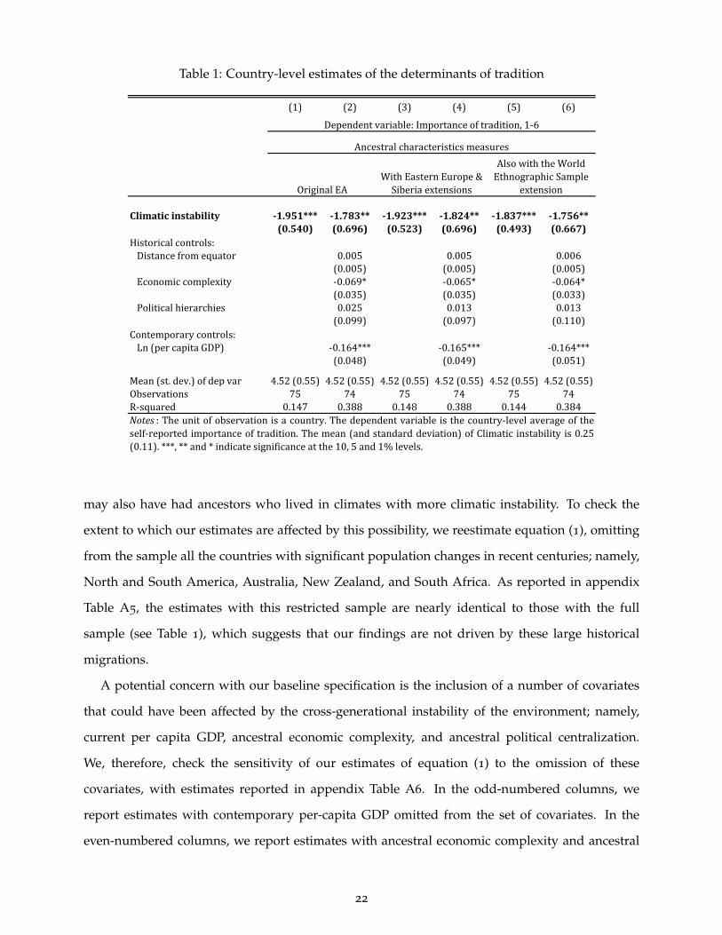
Table 1: Country-level estimates of the determinants of tradition

(1) (2) (3) (4) (5) (6)

Climatic instability -1.951*** -1.783** -1.923*** -1.824** -1.837*** -1.756**(0.540) (0.696) (0.523) (0.696) (0.493) (0.667)

Historical controls:Distance from equator 0.005 0.005 0.006

(0.005) (0.005) (0.005)Economic complexity -0.069* -0.065* -0.064*

(0.035) (0.035) (0.033)Political hierarchies 0.025 0.013 0.013

(0.099) (0.097) (0.110)Contemporary controls:

Ln (per capita GDP) -0.164*** -0.165*** -0.164***(0.048) (0.049) (0.051)

Mean (st. dev.) of dep var 4.52 (0.55) 4.52 (0.55) 4.52 (0.55) 4.52 (0.55) 4.52 (0.55) 4.52 (0.55)Observations 75 74 75 74 75 74R-squared 0.147 0.388 0.148 0.388 0.144 0.384

Dependent variable: Importance of tradition, 1-6

Notes : The unit of observation is a country. The dependent variable is the country-level average of theself-reported importance of tradition. The mean (and standard deviation) of Climatic instability is 0.25(0.11). ***, ** and * indicate significance at the 10, 5 and 1% levels.

Ancestral characteristics measures

Original EAWith Eastern Europe &

Siberia extensions

Also with the World Ethnographic Sample

extension

may also have had ancestors who lived in climates with more climatic instability. To check the

extent to which our estimates are affected by this possibility, we reestimate equation (1), omitting

from the sample all the countries with significant population changes in recent centuries; namely,

North and South America, Australia, New Zealand, and South Africa. As reported in appendix

Table A5, the estimates with this restricted sample are nearly identical to those with the full

sample (see Table 1), which suggests that our findings are not driven by these large historical

migrations.

A potential concern with our baseline specification is the inclusion of a number of covariates

that could have been affected by the cross-generational instability of the environment; namely,

current per capita GDP, ancestral economic complexity, and ancestral political centralization.

We, therefore, check the sensitivity of our estimates of equation (1) to the omission of these

covariates, with estimates reported in appendix Table A6. In the odd-numbered columns, we

report estimates with contemporary per-capita GDP omitted from the set of covariates. In the

even-numbered columns, we report estimates with ancestral economic complexity and ancestral

22

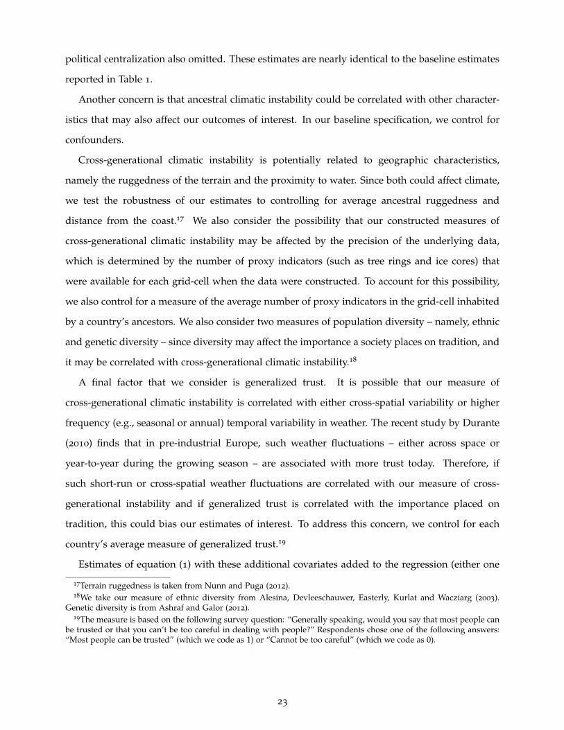
political centralization also omitted. These estimates are nearly identical to the baseline estimates

reported in Table 1.

Another concern is that ancestral climatic instability could be correlated with other character-

istics that may also affect our outcomes of interest. In our baseline specification, we control for

confounders.

Cross-generational climatic instability is potentially related to geographic characteristics,

namely the ruggedness of the terrain and the proximity to water. Since both could affect climate,

we test the robustness of our estimates to controlling for average ancestral ruggedness and

distance from the coast.17 We also consider the possibility that our constructed measures of

cross-generational climatic instability may be affected by the precision of the underlying data,

which is determined by the number of proxy indicators (such as tree rings and ice cores) that

were available for each grid-cell when the data were constructed. To account for this possibility,

we also control for a measure of the average number of proxy indicators in the grid-cell inhabited

by a country’s ancestors. We also consider two measures of population diversity – namely, ethnic

and genetic diversity – since diversity may affect the importance a society places on tradition, and

it may be correlated with cross-generational climatic instability.18

A final factor that we consider is generalized trust. It is possible that our measure of

cross-generational climatic instability is correlated with either cross-spatial variability or higher

frequency (e.g., seasonal or annual) temporal variability in weather. The recent study by Durante

(2010) finds that in pre-industrial Europe, such weather fluctuations – either across space or

year-to-year during the growing season – are associated with more trust today. Therefore, if

such short-run or cross-spatial weather fluctuations are correlated with our measure of cross-

generational instability and if generalized trust is correlated with the importance placed on

tradition, this could bias our estimates of interest. To address this concern, we control for each

country’s average measure of generalized trust.19

Estimates of equation (1) with these additional covariates added to the regression (either one

17Terrain ruggedness is taken from Nunn and Puga (2012).18We take our measure of ethnic diversity from Alesina, Devleeschauwer, Easterly, Kurlat and Wacziarg (2003).

Genetic diversity is from Ashraf and Galor (2012).19The measure is based on the following survey question: “Generally speaking, would you say that most people can

be trusted or that you can’t be too careful in dealing with people?” Respondents chose one of the following answers:“Most people can be trusted” (which we code as 1) or “Cannot be too careful” (which we code as 0).

23

at a time or all together) are reported in appendix Table A7.20 The estimated coefficient for cross-

generational climatic instability remains robust. The coefficient is always negative and significant

and the point estimates remain stable, ranging from about −1.7 to −2.1.

B. Within-country estimates

Our second strategy examines the relationship between historical environmental instability and

the importance of tradition today. Instead of examining country-level variation, we examine

variation across individuals from the WVS, which contains information about the respondent’s

ethnicity, and we measure cross-generational climatic instability at the ethnicity-level. We link the

current ethnicity to the historical ethnicity from the Ethnographic Atlas and estimate the following

equation:

Traditioni,e,c = αc + β Climatic Instabilitye + XiΠ + XeΩ + εi,e,c, (2)

where i denotes an individual, who is a member of ethnic group e and lives in country c.

Traditioni,e,c is the person’s self-reported importance of tradition, which is measured on a 1–6

integer scale and increasing in the importance of tradition. Climatic Instabilitye is our measure

of the variation in temperature across generations in the locations inhabited by the ancestors of

ethnic group e. The standard errors are clustered at the ethnicity level.

Xe denotes the vector of pre-industrial ethnicity-level covariates described above. Xi is a vector

of individual-level covariates that includes a quadratic in age, a gender indicator variable, eight

educational-attainment fixed effects, labor-force-participation fixed effects, a married indicator

variable, ten income-category fixed effects, and fixed effects for the wave of the survey, in which

the individual was interviewed. The specification also includes country fixed effects, αc.

Estimates of equation (2) are reported in Table 2. The odd-numbered columns report estimates

for a version of equation (2) with a parsimonious set of covariates; namely, gender, age, age

squared, and survey-wave fixed effects. In the even-numbered columns, we report estimates for

a version of equation (2) with all covariates. In all specifications, the estimated coefficients for

Climatic Instabilitye are negative and significant. According to the magnitude of the estimates

from column 4, a one-standard-deviation increase in cross-generational climatic instability (0.12)

20Due to space constraints, we only report estimates for the extended sample of 1,292 ethnic groups. The estimatesusing either of the other two ethnicity samples are nearly identical.

24

Table 2: Individual-level estimates of the determinants of tradition, measuring historical instabilityat the ethnicity level

(1) (2) (3) (4) (5) (6)

Climatic instability -0.839*** -0.582** -0.742*** -0.548** -0.772*** -0.561**(0.268) (0.282) (0.276) (0.244) (0.278) (0.248)

Historical ethnicity-level controls:Distance from equator -0.003 -0.004 -0.004

(0.004) (0.003) (0.003)Economic complexity -0.033*** -0.039*** -0.035***

(0.012) (0.012) (0.012)Political hierarchies 0.015 0.026 0.024

(0.028) (0.030) (0.028)Gender, age, age squared yes yes yes yes yes yesSurvey-wave fixed effects yes yes yes yes yes yesOther individual controls no yes no yes no yesCountry fixed effects yes yes yes yes yes yesNumber of countries 75 75 75 75 75 75Number of ethnic groups 186 176 193 183 193 183Mean (st. dev.) of dep var 4.50 (1.41) 4.49 (1.41) 4.50 (1.41) 4.49 (1.41) 4.50 (1.41) 4.49 (1.41)Observations 140,629 127,667 140,681 127,685 139,583 126,630R-squared 0.179 0.181 0.179 0.181 0.179 0.182Notes: The unit of observation is an individual. The dependent variable is a measure of the self-reported importance oftradition. It ranges from 1 to 6 and is increasing in the self-reported importance of tradition. Columns 1, 3 and 5 include aquadratic in age, a gender indicator variable, and survey wave fixed effects. Columns 2, 4 and 6 additionally include eighteducation fixed effects, labor force participation fixed effects, an indicator variable that equals one if the person ismarried, and ten income category fixed effects. Standard errors are clustered at the ethnicity level. The mean (andstandard deviation) of Climatic Instability is 0.27 (0.12). ***, ** and * indicate significance at the 10, 5 and 1% levels.

Dependent variable: Importance of tradition, 1-6

Ancestral characteristics measures

Original EAWith Eastern Europe &

Siberia extensions

Also with the World Ethnographic Sample

extension

is associated with a decrease in the self-reported importance of tradition by 0.12× 0.548 = 0.07,

which is equal to about 0.05 standard deviations of the tradition index.

As the estimates from Tables 1 and 2 show, we obtain very similar estimates irrespective of

which version of the ethnographic data we use. Therefore, for the remainder of the paper, we

take as our baseline sample the extended sample of 1,292 ethnic groups. We do not use the largest

extension, which includes the World Ethnographic Sample, because of the missing information for

the added observations.21 However, all of the estimates that we report are very similar if either of

the other versions is used.21In particular, one of the control variables for some specifications (the year in which the ethnic group was observed

for the data collection) has missing information for 9 of the 17 ethnic groups in the World Ethnographic Sample.

25

5. Examining heterogeneity in the persistence of cultural traits

Our second empirical strategy is to examine the persistence of particular cultural traits and to test

whether it differs systematically depending on the climatic instability across previous generations.

We examine three outcomes that can be measured in a comparable manner over long periods

of time: female labor-force participation (FLFP), the practice of polygamy, and the practice of

consanguineous marriage.

We examine the differential persistence of these cultural practices by estimating the following

regression equation:

Cultural Traitc,t = αr(c) + β1 Cultural Traitc,t−1 + β2 Cultural Traitc,t−1 × Climatic Instabilityc

+Xc,tΠ + Xc,t−1Ω + εc,t (3)

where c indexes countries and t indexes time periods. Period t is the contemporary period (mea-

sured in 2012) and period t− 1 is a historical period that varies depending on the specification.

The dependent variable of interest, Cultural Traitc,t, is our measure of the cultural characteristic

today. We are interested in the relationship between this variable and the cultural trait in the past,

Cultural Traitc,t−1, and how this relationship differs depending on ancestral climatic instability,

Cultural Traitc,t−1 × Climatic Instabilityc. Our interest is in whether the estimated coefficient β2 is

less than zero, which indicates that the cultural trait is less persistent among countries with an

ancestry that experienced a climate that exhibited greater instability between generations.

Equation (3) also includes continent fixed effects, αr(c), which capture broad regional differ-

ences in FLFP, polygamy, and consanguineous marriage. The vector Xc,t contains covariates that

are measured in the contemporary period: log real per-capita GDP as a measure of contempo-

raneous development. When we examine FLFP, we also include a quadratic term to account

for its well-known non-linear relationship with income (Goldin, 1995). Xc,t−1 denotes our vector

of historical covariates: political development (measured by the number of levels of authority

beyond the local community), economic development (measured by complexity and density of

settlements), average distance from the equator of the ancestral homelands, and the direct effect

of the instability of the climate across generations.

26

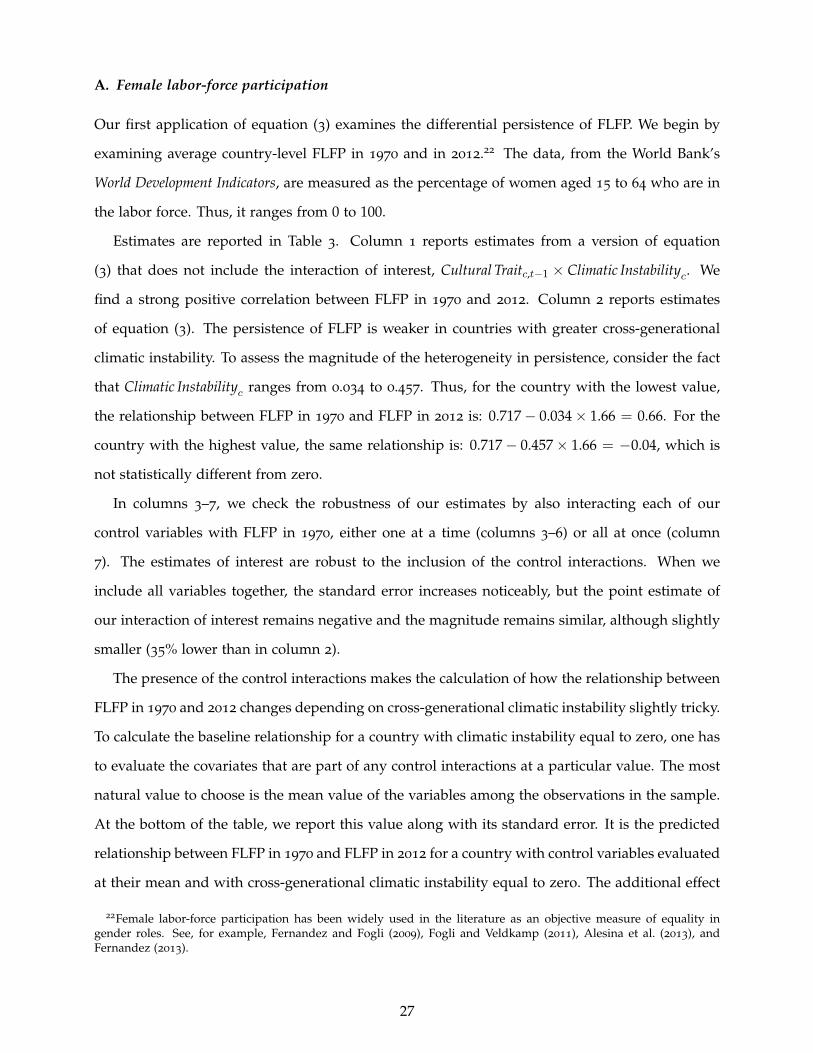
A. Female labor-force participation

Our first application of equation (3) examines the differential persistence of FLFP. We begin by

examining average country-level FLFP in 1970 and in 2012.22 The data, from the World Bank’s

World Development Indicators, are measured as the percentage of women aged 15 to 64 who are in

the labor force. Thus, it ranges from 0 to 100.

Estimates are reported in Table 3. Column 1 reports estimates from a version of equation

(3) that does not include the interaction of interest, Cultural Traitc,t−1 × Climatic Instabilityc. We

find a strong positive correlation between FLFP in 1970 and 2012. Column 2 reports estimates

of equation (3). The persistence of FLFP is weaker in countries with greater cross-generational

climatic instability. To assess the magnitude of the heterogeneity in persistence, consider the fact

that Climatic Instabilityc ranges from 0.034 to 0.457. Thus, for the country with the lowest value,

the relationship between FLFP in 1970 and FLFP in 2012 is: 0.717− 0.034× 1.66 = 0.66. For the

country with the highest value, the same relationship is: 0.717− 0.457× 1.66 = −0.04, which is

not statistically different from zero.

In columns 3–7, we check the robustness of our estimates by also interacting each of our

control variables with FLFP in 1970, either one at a time (columns 3–6) or all at once (column

7). The estimates of interest are robust to the inclusion of the control interactions. When we

include all variables together, the standard error increases noticeably, but the point estimate of

our interaction of interest remains negative and the magnitude remains similar, although slightly

smaller (35% lower than in column 2).

The presence of the control interactions makes the calculation of how the relationship between

FLFP in 1970 and 2012 changes depending on cross-generational climatic instability slightly tricky.

To calculate the baseline relationship for a country with climatic instability equal to zero, one has

to evaluate the covariates that are part of any control interactions at a particular value. The most

natural value to choose is the mean value of the variables among the observations in the sample.

At the bottom of the table, we report this value along with its standard error. It is the predicted

relationship between FLFP in 1970 and FLFP in 2012 for a country with control variables evaluated

at their mean and with cross-generational climatic instability equal to zero. The additional effect

22Female labor-force participation has been widely used in the literature as an objective measure of equality ingender roles. See, for example, Fernandez and Fogli (2009), Fogli and Veldkamp (2011), Alesina et al. (2013), andFernandez (2013).

27

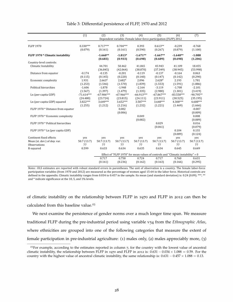
Table 3: Differential persistence of FLFP, 1970 and 2012

(1) (2) (3) (4) (5) (6) (7)

FLFP 1970 0.330*** 0.717*** 0.704*** 0.393 0.613** -0.239 -0.768(0.079) (0.161) (0.161) (0.590) (0.267) (0.879) (1.100)

FLFP 1970 * Climatic instability -1.660** -1.813* -1.671** -1.667** -1.648** -1.088(0.683) (0.933) (0.698) (0.689) (0.698) (1.206)

Country-level controls:Climatic Instability 44.701 50.462 41.065 45.943 41.109 18.455

(36.845) (42.064) (38.870) (37.349) (38.945) (53.998)Distance from equator -0.174 -0.135 -0.201 -0.119 -0.137 -0.164 0.063

(0.115) (0.145) (0.220) (0.140) (0.147) (0.142) (0.290)Economic complexity 1.931 2.663* 2.682* 2.096 2.628* 2.193 1.781

(1.253) (1.546) (1.570) (1.839) (1.553) (1.591) (1.886)Political hierarchies -1.606 -1.878 -1.948 -2.164 -3.119 -1.708 -2.101

(1.567) (1.397) (1.479) (1.335) (2.980) (1.301) (3.419)Ln (per-capita GDP) -71.614*** -67.906*** -67.966*** -66.913*** -67.867*** -83.558*** -90.795**

(24.480) (23.724) (23.815) (24.111) (23.911) (30.525) (35.195)Ln (per-capita GDP) squared 3.822*** 3.649*** 3.652*** 3.587*** 3.648*** 4.308*** 4.608***

(1.255) (1.212) (1.216) (1.232) (1.221) (1.469) (1.666)FLFP 1970 * Distance from equator 0.002 -0.007

(0.006) (0.009)FLFP 1970 * Economic complexity 0.049 0.008

(0.082) (0.089)FLFP 1970 * Political hierarchies 0.029 0.016

(0.061) (0.079)FLFP 1970 * Ln (per capita GDP) 0.104 0.155

(0.089) (0.124)Continent fixed effects yes yes yes yes yes yes yesMean (st. dev.) of dep. var. 50.7 (13.7) 50.7 (13.7) 50.7 (13.7) 50.7 (13.7) 50.7 (13.7) 50.7 (13.7) 50.7 (13.7)Observations 77 77 77 77 77 77 77R-squared 0.599 0.633 0.634 0.635 0.634 0.645 0.649

0.717 0.758 0.724 0.717 0.760 0.631(0.161) (0.236) (0.162) (0.163) (0.166) (0.295)

Dependent variable: Female labor-force participation (FLFP) 2012

Notes : OLS estimates are reported with robust standard errors in parentheses. The unit of observation is a country. The female labor-forceparticipation variables (from 1970 and 2012) are measured as the percentage of women aged 15-64 in the labor force. Historical controls aredefined in the appendix. Climatic instability ranges from 0.034 to 0.457 in the sample. Its mean (and standard deviation) is: 0.24 (0.09). ***, **and * indicate significance at the 10, 5, and 1% levels.

Effect of "FLFP 1970" for mean values of controls and "Climatic instability" = 0

of climatic instability on the relationship between FLFP in 1970 and FLFP in 2012 can then be

calculated from this baseline value.23

We next examine the persistence of gender norms over a much longer time span. We measure

traditional FLFP during the pre-industrial period using variable v54 from the Ethnographic Atlas,

where ethnicities are grouped into one of the following categories that measure the extent of

female participation in pre-industrial agriculture: (1) males only, (2) males appreciably more, (3)

23For example, according to the estimates reported in column 7, for the country with the lowest value of ancestralclimatic instability, the relationship between FLFP in 1970 and FLFP in 2012 is: 0.631− 0.034× 1.088 = 0.59. For thecountry with the highest value of ancestral climatic instability, the same relationship is: 0.631− 0.457× 1.088 = 0.13.

28

equal participation, (4) females appreciably more, and (5) females only.24 To make the traditional

FLFP variable (which ranges from 1 to 5) more comparable with the contemporary measures of

FLFP, we normalize it to also range from 0 to 100. Because traditional female participation in

agriculture is measured in different years for different observations depending, in part, on when

contact was made with the ethnic group, in these regressions we also control for the year in

which the ethnographic data were collected and we allow persistence to differ accordingly. If an

observation’s measure of female participation in pre-industrial agriculture is from a more distant

time period, then it is plausible that we may observe a weaker relationship between the historical

and current measures.

We first examine the average relationship between traditional female participation in agricul-

ture and FLFP in 2012. This is reported in column 1 of Table 4, which shows a strong positive

relationship between the two measures. The point estimate of 0.248 is slightly lower than the

estimate when examining persistence between 1970 and 2012 (column 1 of Table 3). This is not

surprising, since one expects less persistence over a longer time.

Column 2 then reports estimates of equation (3), which allows for differential persistence. We

estimate a negative coefficient for the interaction term, suggesting weaker persistence in countries

with greater ancestral climatic instability. In columns 3–7, we include our set of historical

covariates interacted with traditional female participation in agriculture one control at a time;

in column 8, we include all controls together. The coefficient of interest remains robust.

Within-country differences in the persistence of FLFP

We now examine the continuity of FLFP using within-country, rather than cross-country, varia-

tion. For this, we use yet another data source, IPUMS-International Census data, that records

respondents’ ethnic identity as well as FLFP. This allows us to examine FLFP and link it to

ancestral climatic instability using an individual’s self-reported ethnicity. Although this can only

be done for a much more limited set of countries, the presence of within-country variation across

ethnic groups allows us to obtain estimates using finer variation.

24The original classification in the Ethnographic Atlas distinguishes “differentiated but equal participation” from“equal participation”. Since this distinction is not relevant for our purposes, we combine the two categories into asingle category of equal participation. In addition, for 232 ethnic groups, agriculture was not practiced and thereforethere is no measure of female participation in agriculture. For an additional 315 ethnic groups, information for thevariable is missing. These ethnic groups (547 in total) are omitted from the analysis.

29

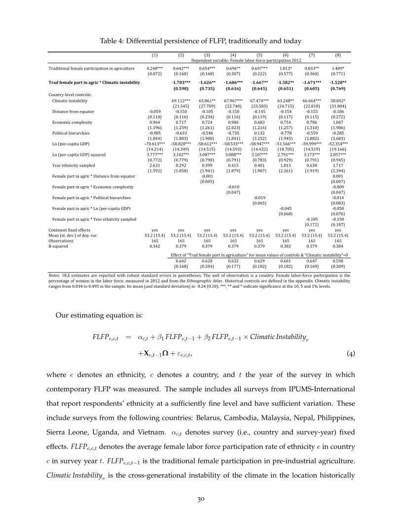
Table 4: Differential persistence of FLFP, traditionally and today

(1) (2) (3) (4) (5) (6) (7) (8)

Traditional female participation in agriculture 0.248*** 0.642*** 0.654*** 0.696** 0.697*** 1.013* 0.833** 1.409*(0.072) (0.168) (0.168) (0.307) (0.222) (0.577) (0.360) (0.771)

Trad female part in agric * Climatic instability -1.703*** -1.626** -1.686*** -1.667** -1.582** -1.671*** -1.528**(0.598) (0.735) (0.616) (0.645) (0.651) (0.605) (0.769)

Country-level controls:Climatic instability 69.112*** 65.861** 67.967*** 67.474*** 63.248** 66.664*** 58.842*

(21.545) (27.709) (22.740) (23.583) (24.715) (22.818) (31.004)Distance from equator -0.059 -0.150 -0.105 -0.150 -0.145 -0.154 -0.155 -0.186

(0.110) (0.116) (0.234) (0.116) (0.119) (0.117) (0.115) (0.272)Economic complexity 0.964 0.717 0.724 0.986 0.683 0.754 0.786 1.067

(1.196) (1.259) (1.261) (2.023) (1.216) (1.257) (1.310) (1.986)Political hierarchies -0.985 -0.633 -0.546 -0.735 0.132 -0.778 -0.559 -0.285

(1.844) (1.883) (1.908) (1.841) (3.252) (1.945) (1.882) (3.683)Ln (per-capita GDP) -70.613*** -58.820*** -58.612*** -58.533*** -58.947*** -51.566*** -59.999*** -52.354***

(14.214) (14.349) (14.515) (14.593) (14.432) (18.705) (14.519) (19.166)Ln (per-capita GDP) squared 3.777*** 3.102*** 3.087*** 3.088*** 3.107*** 2.791*** 3.173*** 2.857***

(0.772) (0.779) (0.790) (0.791) (0.783) (0.929) (0.791) (0.945)Year ethnicity sampled 2.631 0.292 0.399 0.415 0.401 1.015 0.638 1.717

(1.592) (1.858) (1.941) (1.879) (1.907) (2.261) (1.919) (2.394)Female part in agric * Distance from equator -0.001 0.001

(0.005) (0.007)Female part in agric * Economic complexity -0.010 -0.009

(0.047) (0.047)Female part in agric * Political hierarchies -0.019 -0.014

(0.065) (0.083)Female part in agric * Ln (per-capita GDP) -0.045 -0.050

(0.068) (0.076)Female part in agric * Year ethnicity sampled -0.105 -0.150

(0.172) (0.187)Continent fixed effects yes yes yes yes yes yes yes yesMean (st. dev.) of dep. var. 53.2 (15.4) 53.2 (15.4) 53.2 (15.4) 53.2 (15.4) 53.2 (15.4) 53.2 (15.4) 53.2 (15.4) 53.2 (15.4)Observations 165 165 165 165 165 165 165 165R-squared 0.342 0.379 0.379 0.379 0.379 0.382 0.379 0.384

0.642 0.620 0.632 0.629 0.601 0.647 0.598(0.168) (0.204) (0.177) (0.182) (0.182) (0.169) (0.209)

Dependent variable: Female labor-force participation 2012

Notes: OLS estimates are reported with robust standard errors in parentheses. The unit of observation is a country. Female labor-force participation is thepercentage of women in the labor force, measured in 2012 and from the Ethnographic Atlas . Historical controls are defined in the appendix. Climatic instabilityranges from 0.034 to 0.495 in the sample. Its mean (and standard deviation) is: 0.24 (0.10). ***, ** and * indicate significance at the 10, 5 and 1% levels.

Effect of "Trad female part in agriculture" for mean values of controls & "Climatic instability"=0

Our estimating equation is:

FLFPe,c,t = αc,t + β1 FLFPe,t−1 + β2 FLFPe,t−1 × Climatic Instabilitye

+Xe,t−1Ω + εe,c,t, (4)

where e denotes an ethnicity, c denotes a country, and t the year of the survey in which

contemporary FLFP was measured. The sample includes all surveys from IPUMS-International

that report respondents’ ethnicity at a sufficiently fine level and have sufficient variation. These

include surveys from the following countries: Belarus, Cambodia, Malaysia, Nepal, Philippines,

Sierra Leone, Uganda, and Vietnam. αc,t denotes survey (i.e., country and survey-year) fixed

effects. FLFPe,c,t denotes the average female labor force participation rate of ethnicity e in country

c in survey year t. FLFPe,c,t−1 is the traditional female participation in pre-industrial agriculture.

Climatic Instabilitye is the cross-generational instability of the climate in the location historically

30

Table 5: Ethnicity-level estimates of the differential persistence of FLFP, traditionally and today

(1) (2) (3) (4) (5) (6) (7)

Traditional female participation in agriculture 0.157* 0.400** 0.406** 0.685*** 0.372* 3.225 4.280*(0.082) (0.153) (0.189) (0.254) (0.217) (2.273) (2.501)

Trad female part in agric * Climatic instability -1.268* -1.256* -1.059 -1.268* -1.362* -1.042(0.722) (0.678) (0.688) (0.724) (0.742) (0.653)

Ethnicity-level controls:Climatic instability 55.165 54.202 41.809 55.406 60.687* 42.052

(34.924) (33.472) (33.328) (34.965) (36.381) (32.735)Distance from equator 0.045 -0.067 -0.050 -0.053 -0.068 -0.068 -0.028

(0.131) (0.148) (0.224) (0.147) (0.147) (0.147) (0.248)Economic complexity 0.935 0.824 0.831 3.469* 0.828 0.633 4.690**

(1.000) (0.918) (0.921) (2.041) (0.925) (0.954) (2.240)Political hierarchies -0.608 -0.250 -0.253 -0.662 -0.582 -0.129 -3.283

(1.194) (1.206) (1.216) (1.219) (2.236) (1.223) (2.858)Year ethnicity sampled -3.437 0.011 -0.006 0.119 0.127 0.820 2.088

(2.492) (3.387) (3.330) (3.486) (3.443) (3.365) (3.616)Female part agric * Distance from equator -0.000 -0.001

(0.005) (0.006)Female part agric * Economic complexity -0.052* -0.080**

(0.031) (0.037)Female part agric * Political hierarchies 0.008 0.059

(0.034) (0.046)Female part agric * Year ethnicity sampled -1.452 -1.873

(1.131) (1.222)Country-survey-year fixed effects yes yes yes yes yes yes yesMean (st. dev.) of dep. var. 54.8 (22.37) 54.8 (22.37) 54.8 (22.37) 54.8 (22.37) 54.8 (22.37) 54.8 (22.37) 54.8 (22.37)Number of ethnicities 109 109 109 109 109 109 109Observations 211 211 211 211 211 211 211R-squared 0.478 0.492 0.492 0.499 0.492 0.496 0.509

0.400 0.398 0.354 0.396 0.436 0.350(0.151) (0.148) (0.141) (0.155) (0.165) (0.155)

Dependent variable: Average female labor-force participation rate today

Notes: OLS estimates are reported with standard errors clustered at the ethnicity level in parentheses. The unit of observation is an ethnicity in a givencountry/year. Female labor-force participation is the percentage of women in the labor force. The countries (and their survey years) included in the sampleare Belarus (1999), Cambodia 1998, 2008), Malaysia (1970, 1980, 1991, 2000), Nepal (2001), Philippines (1990), Sierra Leone (2004), Uganda (1991, 2002),and Vietnam (1989, 1999, 2009). Climatic instability ranges from 0.034 to 0.516 in the sample. Its mean (and standard deviation) is: 0.19 (0.10). ***, ** and *indicate significance at the 10, 5 and 1% levels.

Effect of "Trad female part in agric" for mean values of controls & "Climatic instability"=0

inhabited by ethnic group e. Xe,c,t−1 denotes historical controls measured at the ethnicity level and

αc,t denotes country-survey-year fixed effects. The standard errors are clustered at the ethnicity

level.

Estimates of equation (4) are reported in Table 5. Although the estimates are less precise than

the country-level estimates, they do confirm the findings from the cross-country analysis. First, we

find persistence between female participation in agriculture historically and FLFP today (column

1). Second, we find that this persistence is weaker for those ethnicities with greater instability

of the climate across previous generations (column 2). In addition, the finding is robust to the

inclusion of the ethnicity-level historical controls and their interactions with historical female

participation in agriculture, either individually or together (columns 3–7).

31

B. Polygamy

Our next estimates of equation (3) examine the differential persistence of polygamy. We view this

as an informative complement to FLFP, since polygamy has been declining, while FLFP has been

increasing. We measure the traditional presence of polygamy using information from variable

v9 in the Ethnographic Atlas.25 We measure the prevalence of polygamy today using data from

the OECD Gender, Institutions and Development Database. The variable we use is a country-level

indicator that equals one if having more than one spouse is accepted or legal.

Estimates of the relationship between the traditional prevalence of polygamy and the practice

today are reported in column 1 of Table 6. The remaining columns report estimates of the full

version of equation (3). We find that, as was the case for FLFP, the coefficient for the interaction

term, β2, is negative and significant. The persistence of polygamy is weaker in countries where the

climate faced by the populations’ ancestors was more unstable from one generation to the next.

This is true without (column 2) or with (columns 3–8) the inclusion of the covariates interacted

with the historical measure of polygamy. Although we lose significance in two of the seven

specifications, the coefficient remains negative and of a similar magnitude in all specifications.

C. Consanguineous marriage

Another traditional practice that, like polygamy, has been declining over time is consanguineous

marriage, which is defined as a marriage between two people who are related as second cousins

or closer, and commonly referred to as “cousin marriage”. In some countries, the practice has

declined over time. In others, it continues to persist and still accounts for a large fraction of

marriages (Bittles and Black, 2010).

We measure the presence of the practice today using data on contemporaneous consan-

guineous marriages taken from Schulz (2017). Our measure is the proportion of all marriages

that are consanguineous. The traditional presence of consanguineous marriage is calculated from

the variable v25 of the Ethnographic Atlas26 which is the proportion of the population today with

25The categories coded in the Ethnographic Atlas are: independent nuclear monogamous, polygyny, preferentialsororal living in the same dwelling, preferential sororal living in a separate dwelling, non-sororal living in separatedwelling, non-sororal living in the same dwelling, polyandry, and no information.

26The original coding of the variable has 14 categories for different forms of cousin marriage preference when cousinmarriages are preferred to non-cousin marriages. The fifteenth category is for “No preferred cousin marriages”. Fromvariable v25, we create an indicator variable that equals 0 if the ethnicity has “No preferred cousin marriages” and 1

if it has a preferred cousin marriage of any type.

32

Table 6: Differential persistence of polygamy, traditionally and today

(1) (2) (3) (4) (5) (6) (7) (8)

Traditional polygamy, 0-1 0.324*** 0.845*** 1.182*** 0.612** 1.786*** 1.862*** 3.159* 2.708*(0.122) (0.212) (0.220) (0.290) (0.368) (0.666) (1.683) (1.599)

Traditional polygamy * Climatic instability -2.177** -1.173 -2.153** -2.071*** -1.805* -2.171** -1.205(0.878) (0.747) (0.864) (0.765) (0.914) (0.877) (0.753)

Country-level controls:Climatic instability 2.363*** 1.457*** 2.399*** 2.184*** 1.975*** 2.383*** 1.429***

(0.667) (0.476) (0.659) (0.511) (0.681) (0.666) (0.453)Distance from equator -0.004 -0.006* 0.008** -0.006* -0.005 -0.006** -0.006* 0.004*

(0.003) (0.003) (0.003) (0.003) (0.003) (0.003) (0.003) (0.002)Economic complexity -0.010 -0.013 -0.019 -0.042 -0.014 -0.014 -0.013 -0.033*

(0.020) (0.021) (0.019) (0.025) (0.021) (0.020) (0.020) (0.020)Political hierarchies -0.033 -0.033 -0.020 -0.034 0.186*** -0.030 -0.030 0.143***

(0.039) (0.036) (0.033) (0.036) (0.059) (0.035) (0.036) (0.053)Ln (per capita GDP) -0.034 -0.043 -0.043 -0.043 -0.042 0.065 -0.045 0.010

(0.031) (0.031) (0.030) (0.031) (0.030) (0.064) (0.032) (0.066)Year ethnicity sampled -0.104** -0.109** -0.122*** -0.109** -0.108** -0.118** 1.091 0.152

(0.044) (0.045) (0.045) (0.045) (0.045) (0.046) (0.855) (0.950)Traditional polygamy * Distance from equator -0.018*** -0.013***

(0.005) (0.005)Traditional polygamy * Economic complexity 0.038 0.018

(0.034) (0.030)Traditional polygamy * Political hierarchies -0.262*** -0.197***

(0.077) (0.074)Traditional polygamy * Log (per-capita GDP) -0.122* -0.060

(0.072) (0.073)Traditional polygamy * Year sampled -1.203 -0.274

(0.867) (0.956)Continent fixed effects yes yes yes yes yes yes yes yesMean (st. dev.) of dep. var. 0.44 (0.41) 0.44 (0.41) 0.44 (0.41) 0.44 (0.41) 0.44 (0.41) 0.44 (0.41) 0.44 (0.41) 0.44 (0.41)Observations 109 109 109 109 109 109 109 109R-squared 0.539 0.574 0.602 0.576 0.597 0.581 0.577 0.616

0.845 0.760 0.846 0.903 0.795 1.049 0.851(0.212) (0.188) (0.212) (0.199) (0.215) (0.262) (0.232)

Dependent variable: Indicator variable for the practice of polygamy today, 0/1

Notes: OLS estimates are reported with robust standard errores in brackets. The unit of observation is a country. Polygamy is an indicator variable that equalsone if having more than one spouse is an accepted or legal practice in the country. Climatic instability ranges from 0.052 to 0.495 in the sample. Its mean (andstandard deviation) is: 0.21 (0.09). ***, ** and * indicate significance at the 10, 5 and 1% levels.

Effect of "Traditional polygamy" for mean values of controls and "Climatic instability" = 0

ancestors for whom consanguineous marriage was the preferred form. Thus, both measures range

from 0 to 100.

The estimate of the persistence of consanguineous marriage is reported in column 1 of Table

7. Estimates of the differential persistence of the trait by cross-generational climatic instability

are reported in columns 2–8. As above, column 2 reports the baseline estimates, while columns

3–8 report estimates with each of the baseline control variables interacted with the traditional

prevalence of the practice, either individually or together.27 The coefficient for the interaction

term, β2, is negative and significant in all specifications. Thus, the persistence of consanguineous

marriage is weaker in countries where the climate of the population’s ancestors was more unstable

33

Table 7: Differential persistence of consanguineous marriage, traditionally and today

(1) (2) (3) (4) (5) (6) (7) (8)

Traditional consanguineous marriage, 0-100 0.178*** 0.401*** 0.402*** 0.179 0.388 0.210 0.390*** -0.104(0.066) (0.086) (0.115) (0.438) (0.262) (0.516) (0.080) (0.884)

Trad consanguineous marriage * Climatic instability -1.310** -1.308** -1.323** -1.322** -1.221** -1.327** -1.196**(0.556) (0.566) (0.572) (0.648) (0.491) (0.550) (0.585)

Country-level controls:Climatic instability 34.223 34.105 40.472 34.771 34.960 37.643 47.573

(22.269) (24.022) (33.221) (27.336) (23.636) (22.524) (39.334)Distance from equator 0.112 0.052 0.053 0.045 0.054 0.075 0.036 0.009

(0.146) (0.155) (0.161) (0.166) (0.159) (0.138) (0.155) (0.187)Economic complexity 0.319 -2.984* -2.987 -5.847 -3.034 -2.443 -3.170* -6.558

(1.833) (1.755) (1.782) (6.574) (1.944) (1.639) (1.740) (6.538)Political hierarchies -1.904 -0.492 -0.489 -0.272 -0.639 -0.833 -0.221 0.813

(2.683) (2.598) (2.671) (2.663) (4.291) (3.127) (2.656) (4.784)Ln (per-capita GDP) -3.139 -4.805* -4.803* -4.427* -4.824 -5.432 -5.120* -5.318

(2.761) (2.699) (2.763) (2.204) (2.940) (3.630) (2.737) (3.413)Years between current and historical periods 0.001 0.001 0.001 0.000 0.001 0.000 -0.031 -0.045

(0.003) (0.003) (0.003) (0.002) (0.003) (0.002) (0.042) (0.045)Trad consanguineous * Distance from equator -0.000 0.001

(0.003) (0.003)Trad consanguineous * Economic complexity 0.034 0.051

(0.068) (0.079)Trad consanguineous * Political hierarchies 0.004 -0.027

(0.073) (0.078)Trad consanguineous * Log (per-capita GDP) 0.019 0.023

(0.053) (0.055)Trad consanguineous * Years between 0.000 0.000

(0.000) (0.000)Continent fixed effects yes yes yes yes yes yes yes yesMean (st. dev.) of dep. var. 12.8 (16.4) 12.8 (16.4) 12.8 (16.4) 12.8 (16.4) 12.8 (16.4) 12.8 (16.4) 12.8 (16.4) 12.8 (16.4)Observations 60 60 60 60 60 60 60 60R-squared 0.662 0.702 0.702 0.705 0.702 0.703 0.704 0.711

0.401 0.400 0.402 0.403 0.393 0.455 0.469(0.086) (0.087) (0.089) (0.092) (0.085) (0.126) (0.150)

Dependent variable: Percent of marriages that are consanguineous today, 0-100

Notes: OLS estimates are reported with robust standard errores in brackets. The unit of observation is a country. The dependent variable is the proportion of total marriages thatare consanguineous. The measure is taken by Schulz (2017). Climatic instability ranges from 0.052 to 0.457 in the sample. Its mean (and standard deviation) is: 0.25 (0.10). ***, **and * indicate significance at the 10, 5 and 1% levels.

Effect of "Traditional consanguineous marriage" for mean values of controls & "Climatic instability" = 0

across previous generations.

6. Ancestral climatic instability and the persistence of cultural traits: Evidence from

U.S. immigration

Our next set of tests uses immigration as a natural setting in which to examine the importance

of tradition and the differential persistence of cultural traits. We examine the extent to which

traditional practices persist amongst the descendants of immigrants to the United States and

whether this persistence is predicted by the historical instability of the group’s climate. We

examine two traditional practices that are universal in the origin countries: marrying someone

from the same nationality and speaking one’s mother tongue at home.

27In the Schulz (2017) data, the prevalence of consanguineous marriage is measured in different years in the late 20thcentury. Given this, in the regression equations, rather than controlling for the year of measurement in the historicalethnographic data, we control for the difference between the year of measurement in the contemporary period and theyear of measurement in the historical period.

34

A. Within-group marriage

In all countries, the traditional practice is to marry someone from your own country. After

migrating to the United States, for the children of immigrants continuing this tradition is difficult.

The importance of the practice to both the parents and their children will affect the extent to which

the children marry someone with the same heritage. Of course, other factors will also affect this

decision, such as the availability of potential partners from one’s own cultural background or the

cultural distance between the origin country and the United States. We are, therefore, careful to

control for these factors in the empirical analysis.

Our analysis examines the probability that the children of immigrants marry someone from

the country of origin.28 Before turning to formal estimates, we first examine the raw correlations

between within-group marriage and climatic instability across previous generations. To do this,

we use a sample of married women with at least one parent who was born outside the United

States. A wife’s origin country can be identified by either her mother or father’s country of birth.

In the empirical analysis, we will report estimates separately for both cases. In our examination

of the raw data, we use the mother’s country of birth. We identify a wife’s husband as being

of the same ancestry as her if he, or one of his parents, or both, were born in the wife’s origin

country.

The relationship between the fraction of wives from an origin country who have married

someone with the same ancestry is shown in Figures 6a and 6b. Figure 6a shows the relationship

with the observations labelled with their three-digit country ISO code. Figure 6b reports the

relationship with countries denoted by circles, where the size of the circle is proportional to the

number of wives in the sample who are from that origin country. From the figures, a negative

relationship between the two measures is apparent. Women from origin countries with more

cross-generational climatic instability are less likely to have a spouse from the same country.

We now turn to a more formal examination of this relationship by estimating the following

equation:

IIngroup Marriagei,c = α+ β Climatic Instabilityc + XcΠ + XiΦ + εi,c, (5)

where i indexes married women or men (depending on the sample) who were born in the U.S., but

28Information on the country of origin of individuals is available for the recent period from the March Supplement ofthe Current Population Survey (CPS). Beginning in 1994, for all individuals who were born in the United States, the CPSbegan recording both parents’ countries of birth. In our analysis, we use each of the 21 available waves.

35

AFGALB

ARM

ATG

AUS

AUT

BEL

BGD

BGR

BHS

BLR

BLZ

BMU

BOLBRA

BRB

CAN

CHE

CHL

CHN

COL

CPV

CRI

CUB

CYP

CZE

DEU

DMA

DNK

DOM DZA

ECU

EGY ESP

ETH

FIN

FJI

FRAGBRGEOGHA

GRC

GRD

GTM

GUYHND

HRV

HTI

HUN

IDN

IND

IRL

IRN

IRQ

ISL

ISR

ITA

JAM

JOR

JPN

KEN

KHM

KOR

LAO

LBN

LKA

LTU

LVAMAR

MEX

MKD

MYSNGA

NICNLD

NOR

NZL

PAK

PAN

PER

PHL

POL

PRI

PRT

PRY

ROU

RUS

SAUSDN

SGP

SLVSVK

SWE

THA

TON

TTO

TUR

UGA

UKR

URY

VEN

VNM

WSM

YEM

ZAF0.2

.4.6

.81

Husband fro

m the s

am

e c

ountr

y o

f origin

0 .1 .2 .3 .4 .5Climatic instability

(coef = −1.35, t = −2.79)

(a) Bivariate relationship with names of country of origin shown

0.2

.4.6

.81

Husband fro

m the s

am

e c

ountr

y o

f origin

0 .1 .2 .3 .4 .5Climatic instability

(coef = −1.35, t = −2.79)

(b) Bivariate relationship where the circle size denotes the number of individuals from the countryof origin in the sample

Figure 6: Bivariate relationship between women marrying men from their country of origin andcross-generational climatic instability

36

whose parents are immigrants who were born outside the U.S., and c indexes the origin country

of the individual’s parents. The outcome of interest, I Ingroup Marriagei,c , is an indicator variable that

equals one if an individual’s spouse was born in origin country c or if his or her mother or

father was born in country c. The vector of country-level covariates, Xc, includes the natural log

of the current per-capita GDP in the country of origin (measured in the survey year), and all

the historical ethnicity characteristics from that country (distance from the equator, a measure

of economic complexity, and a measure of political sophistication). We also include the genetic

distance between the country of origin and the United States as a proxy of cultural distance,

which could affect outgroup marriage.29

The following individual-level covariates, Xi, are included in all specifications: a quadratic in

age, educational-attainment fixed effects (less than high school, high school only, and more than

high school), metropolitan-area fixed effects, rural/urban indicator, and survey-year fixed effects.

We also control for the fraction of the population in the same metropolitan area as the individual

who are first- or second-generation immigrants from the individual’s country of origin.30

Estimates of equation (5) are reported in Table 8. In columns 1 and 2, the unit of observation is

a married woman, while in columns 3 and 4, it is a married man. In columns 1 and 3, we define

the origin country by the birthplace of the person’s father, while in columns 2 and 4, we define

it by the birthplace of the mother. Across all four specifications, we find a negative relationship

between cross-generational climatic instability and the probability of marrying someone of one’s

own ancestry. The magnitudes and significance appear to be greater for the sample of married

women than for the sample of married men. The effects also appear stronger when we define a

person’s origin country using the mother than when using the father. According to the estimates

for married women from column 2, a one-standard-deviation increase in cross-generational

climatic instability is associated with a decrease in ingroup marriage by 0.044, equal to 14 percent

of the mean of the independent variable and 9 percent of its standard deviation.31 When we look

at the estimates for married men from column 4, we find that a one-standard-deviation increase in

cross-generational climatic instability is associated with a decrease in ingroup marriage by 0.022,

which is 8 percent of the mean of the dependent variable and 5 percent of its standard deviation.

29The measure is taken from Spolaore and Wacziarg (2009).30For individuals who do not live in a metropolitan area, we use the fraction of the population living in non-

metropolitan areas within the same state.31Descriptive statistics are reported in appendix Table A1.

37

Table 8: Women and men marrying a spouse from their origin country, using CPS 1994–2014

(1) (2) (3) (4)

Origin country identified from

father

Origin country identified from

mother

Origin country identified from

father

Origin country identified from

mother

Climatic instability -0.274* -0.492*** -0.103 -0.250*(0.156) (0.178) (0.138) (0.148)

Country-level controls:Distance from equator -0.006** -0.005 -0.008*** -0.009***

(0.003) (0.003) (0.003) (0.003)Economic complexity 0.009 0.019 -0.010 -0.021

(0.026) (0.035) (0.039) (0.037)Political hierarchies 0.089*** 0.084*** 0.092** 0.085**

(0.027) (0.029) (0.037) (0.037)Ln (per-capita GDP) -0.005 -0.022 -0.003 -0.004

(0.030) (0.033) (0.036) (0.035)Genetic distance from the United States 0.031 0.010 0.011 -0.010

(0.046) (0.053) (0.043) (0.044)Fraction of population in location who are first- or second- 3.314*** 3.533*** 3.071*** 3.409***

generation immigrants from their country of origin (0.489) (0.627) (0.504) (0.483)Individual-level controls yes yes yes yesNumber of countries 108 105 110 105Mean (st. dev.) of dependent variable 0.33 (0.47) 0.32 (0.47) 0.28 (0.45) 0.29 (0.45)Observations 36,082 34,045 38,419 35,639R-squared 0.239 0.254 0.223 0.245

Dependent variable: Indicator varible for spouse being from their origin country

Notes : OLS estimates are reported with standard errors clustered at the country-of-origin level in parentheses. In columns 1 and 2, the unit ofobservation is a daughter of at least one immigrant parent who is married at the time of the survey. In columns 1 and 2, the dependent variable isan indicator variable that equals one if the woman is married to someone with the same ancestry (i.e., an individual born in the country or with atleast one parent who was born in the country). In columns 3 and 4, the unit of observation is a son of at least one immigrant parent who ismarried at the time of the survey. In columns 3 and 4, the dependent variable is an indicator variable that equals one if the man is married tosomeone with the same ancestry. The country of origin of the observation is defined by the country of birth of the father in columns 1 and 3 andthe country of birth of the mother in column 2 and 4. The following controls are included in all specifications: a quadratic in age, two indicatorvariables for educational attainment (less than high school and high school), metropolitan-area fixed effects, and survey-year fixed effects. Themean and standard deviation of climatic instability is 0.29 (0.09). ***, ** and * indicate significance at the 10, 5 and 1% levels.

Sample: Married women Sample: Married men

B. Is a foreign language spoken at home?

The second indicator of the persistence of tradition among descendants of immigrants is whether

or not English is spoken at home. In all origin countries, people speak one of the vernaculars

of their country. However, since the children of migrants who are born in the United States are

almost always fluent in English, they face the decision of whether to continue speaking their

traditional language at home. We thus examine, as a revealed measure of the importance of

maintaining tradition, the extent to which a foreign language is spoken at home among the

children of immigrants. If so, it indicates that the children of the immigrants were taught their

origin language, which is a sign of the parents and children valuing their tradition. It also means

that the origin language is valued enough for it to be spoken within the household. Since the

ease with which parents can learn English will be an important determinant of whether children

speak English at home, we always control for a measure of the linguistic distance of the origin

38

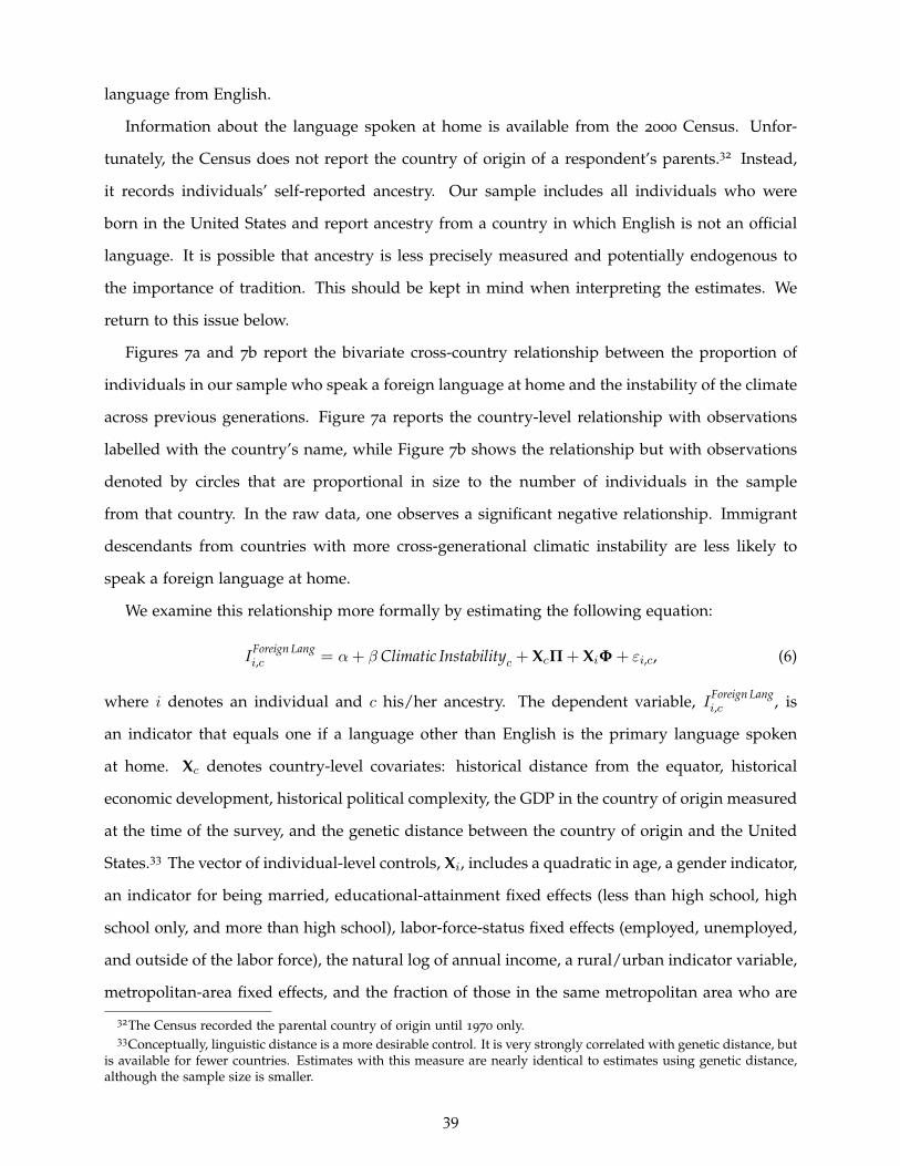
language from English.

Information about the language spoken at home is available from the 2000 Census. Unfor-

tunately, the Census does not report the country of origin of a respondent’s parents.32 Instead,

it records individuals’ self-reported ancestry. Our sample includes all individuals who were

born in the United States and report ancestry from a country in which English is not an official

language. It is possible that ancestry is less precisely measured and potentially endogenous to

the importance of tradition. This should be kept in mind when interpreting the estimates. We

return to this issue below.

Figures 7a and 7b report the bivariate cross-country relationship between the proportion of

individuals in our sample who speak a foreign language at home and the instability of the climate

across previous generations. Figure 7a reports the country-level relationship with observations

labelled with the country’s name, while Figure 7b shows the relationship but with observations

denoted by circles that are proportional in size to the number of individuals in the sample

from that country. In the raw data, one observes a significant negative relationship. Immigrant

descendants from countries with more cross-generational climatic instability are less likely to

speak a foreign language at home.

We examine this relationship more formally by estimating the following equation:

IForeign Langi,c = α+ β Climatic Instabilityc + XcΠ + XiΦ + εi,c, (6)

where i denotes an individual and c his/her ancestry. The dependent variable, IForeign Langi,c , is

an indicator that equals one if a language other than English is the primary language spoken

at home. Xc denotes country-level covariates: historical distance from the equator, historical

economic development, historical political complexity, the GDP in the country of origin measured

at the time of the survey, and the genetic distance between the country of origin and the United

States.33 The vector of individual-level controls, Xi, includes a quadratic in age, a gender indicator,

an indicator for being married, educational-attainment fixed effects (less than high school, high

school only, and more than high school), labor-force-status fixed effects (employed, unemployed,

and outside of the labor force), the natural log of annual income, a rural/urban indicator variable,

metropolitan-area fixed effects, and the fraction of those in the same metropolitan area who are

32The Census recorded the parental country of origin until 1970 only.33Conceptually, linguistic distance is a more desirable control. It is very strongly correlated with genetic distance, but

is available for fewer countries. Estimates with this measure are nearly identical to estimates using genetic distance,although the sample size is smaller.

39

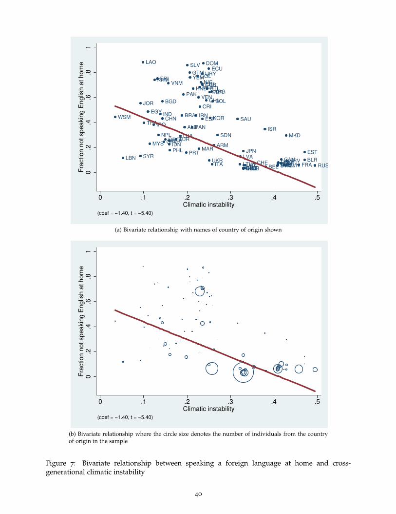
ALB

ARG

ARM

AUT BEL

BGD

BGRBLR

BOL

BRA

CANCHE

CHL

CHN

COL

CPV

CRI

CUB

CZEDEUDNK

DOMECU

EGY

ERI

ESP

EST

ETH

FIN FRA

GRC

GTM

HND

HRV

HTI

HUN

IDN

IND IRN

IRQ

ISL

ISR

ITA

JOR

JPN

KHM

KOR

LAO

LBN

LKA

LTULUX

LVA

MAR

MEX

MKD

MYS

NIC

NLDNOR

NPL

PAK

PAN

PER

PHL

POL

PRI

PRT

RUS

SAU

SDN

SLV

SVKSVNSWE

SYR

THA

TUR

UKR

URY

VEN

VNM

WSM

YEM

0.2

.4.6

.81

Fra

ction n

ot speakin

g E

nglis

h a

t hom

e

0 .1 .2 .3 .4 .5Climatic instability

(coef = −1.40, t = −5.40)

(a) Bivariate relationship with names of country of origin shown

0.2

.4.6

.81

Fra

ction n

ot speakin

g E

nglis

h a

t hom

e

0 .1 .2 .3 .4 .5Climatic instability

(coef = −1.40, t = −5.40)

(b) Bivariate relationship where the circle size denotes the number of individuals from the countryof origin in the sample

Figure 7: Bivariate relationship between speaking a foreign language at home and cross-generational climatic instability

40

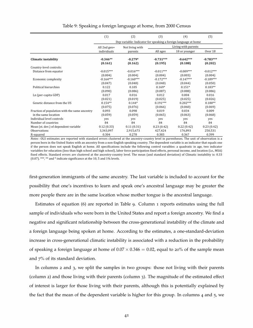
Table 9: Speaking a foreign language at home, from 2000 Census

(1) (2) (3) (4) (5)

All ages 18 or younger Over 18

Climatic instability -0.346** -0.279* -0.731*** -0.642*** -0.783***(0.161) (0.162) (0.195) (0.188) (0.202)

Country-level controls:Distance from equator -0.015*** -0.016*** -0.011*** -0.009*** -0.012***

(0.004) (0.004) (0.004) (0.003) (0.004)Economic complexity -0.164*** -0.160*** -0.172*** -0.147*** -0.189***

(0.047) (0.048) (0.048) (0.044) (0.050)Political hierarchies 0.122 0.105 0.169* 0.151* 0.183**

(0.090) (0.086) (0.087) (0.088) (0.086)Ln (per-capita GDP) 0.017 0.016 0.012 0.004 0.016

(0.021) (0.019) (0.025) (0.025) (0.026)Genetic distance from the US 0.154** 0.144* 0.191*** 0.202*** 0.180**

(0.075) (0.076) (0.066) (0.060) (0.069)Fraction of population with the same ancestry 0.093 0.098 0.019 0.034 0.009

in the same location (0.059) (0.059) (0.065) (0.063) (0.068)Individual level controls yes yes yes yes yesNumber of countries 84 84 84 84 84Mean (st. dev.) of dependent variable 0.12 (0.33) 0.11 (0.31) 0.23 (0.42) 0.22 (0.42) 0.23 (0.42)Observations 3,343,097 2,915,673 427,424 176,893 250,531R-squared 0.304 0.278 0.383 0.367 0.399

Dep variable: Indicator for speaking a foreign language at home

All 2nd gen+ individuals

Not living with parents

Living with parents

Notes : OLS estimates are reported with standard errors clustered at the ancestry-country level in parentheses. The unit of observation is aperson born in the United States with an ancestry from a non-English speaking country. The dependent variable is an indicator that equals oneif the person does not speak English at home. All specifications include the following control varaibles: a quadratic in age, two indicatorvariables for education (less than high school and high school), labor force participation fixed effects, personal income, and location (i.e., MSA)fixed effects. Standard errors are clustered at the ancestry-country level. The mean (and standard deviation) of Climatic instability is: 0.33(0.07). ***, ** and * indicate significance at the 10, 5 and 1% levels.

first-generation immigrants of the same ancestry. The last variable is included to account for the

possibility that one’s incentives to learn and speak one’s ancestral language may be greater the

more people there are in the same location whose mother tongue is the ancestral language.

Estimates of equation (6) are reported in Table 9. Column 1 reports estimates using the full

sample of individuals who were born in the United States and report a foreign ancestry. We find a

negative and significant relationship between the cross-generational instability of the climate and

a foreign language being spoken at home. According to the estimates, a one-standard-deviation

increase in cross-generational climatic instability is associated with a reduction in the probability

of speaking a foreign language at home of 0.07× 0.346 = 0.02, equal to 20% of the sample mean

and 7% of its standard deviation.

In columns 2 and 3, we split the samples in two groups: those not living with their parents

(column 2) and those living with their parents (column 3). The magnitude of the estimated effect

of interest is larger for those living with their parents, although this is potentially explained by

the fact that the mean of the dependent variable is higher for this group. In columns 4 and 5, we

41

further split the sample of children living with their parents by age: those who are 18 or younger

(column 4) and those who are older than 18 (column 5). We find that the negative relationship

between cross-generational climatic instability and speaking a foreign language at home is similar

for both groups, although the effect is slightly larger in magnitude for those over 18.34

In the previous analysis of the determinants of ingroup marriage, we were able to use a

parent’s country of birth as a measure of ancestry. However, for this analysis, due to data

availability, we must use self-reported ancestry. It is possible that this is imprecisely measured

and potentially endogenous to the importance of tradition. It is unclear how this could bias the

results. On the one hand, the estimates could be biased towards zero due to classical measurement

error. On the other hand, if those who value tradition more are more likely to report a foreign

ancestry, then this could result in nonclassical measurement error. Since the observed sample will

tend to disproportionately include these observations, if the estimated effect of ancestral climatic

instability is particularly strong for this group, then our estimates would be biased away from

zero. Given this concern, we check the robustness of our findings to estimates that give equal

weight to each origin country. Appendix Table A11 reports estimates of a variant of equation (6),

in which the unit of observation is an origin country and a location of residence. The estimates

are qualitatively identical to those in Table 9.

7. Climatic instability and the persistence of cultural traits: Evidence from Indigenous

populations

A potential concern with our analysis involving immigrants is that immigrants are not a represen-

tative subsample of the populations in the origin countries. Migrants are a selected group, which

is problematic if the nature of selection varies systematically with the climatic instability of the

origin country. We, therefore, undertake a fourth exercise that examines populations that are not

immigrants but, like immigrants, face pressure to change their traditions and customs. These are

the Indigenous populations of the United States and Canada. Like immigrants, they are minority

groups whose cultural traditions differ from those of the dominant population. However, unlike

immigrants, they are not a product of selection from migration.

34In our baseline specification, we omit from the sample individuals whose ancestral country has English asan official language. As we report in appendix Table A10, the estimates are nearly identical if we include theseobservations.

42

As in our analysis of the children of immigrants, we take the language spoken at home as

a measure of the continuity and maintenance of tradition. Thus, we estimate the relationship

between the cross-generational climatic instability faced by the ancestors of today’s Indigenous

populations and the extent to which they speak their traditional language today. Within the

United States and Canada, there is significant variation in the extent to which Indigenous

populations have maintained their language. Many have lost their original language completely,

while others, such as the Navajo, have done very well at retaining it (Arthur and Diamond, 2011).

The sample from the United States, which is taken from the U.S. Census, includes all individu-

als who identify themselves as Native Americans. We use data from all comparable Census years

for which data are available (1930, 1990, and 2000).35 We link an individual to a Native American

ethnic group using self-reported tribal affiliation. Using information on the traditional location

of each ethnic group from the Ethnographic Atlas, we then assign a measure of cross-generational

climatic instability to each tribe.

Figure 8 reports a map showing the ethnic groups in our sample (according to the Ethnographic

Atlas classification). Also shown are the climatic grid-cells and the categories of the cross-

generational instability measure. One observes significant variation in cross-generational climatic

instability, making the Native American experience a useful setting to examine the importance of

tradition and persistence of culture.

Our estimating equation is as follows:

INative Langi,e,k = αk + β Climatic Instabilitye + XeΠ + XiΦ+εi,e,k, (7)

where i denotes an individual, e his/her ethnic group, and k a location of residence (metropolitan

area). The dependent variable, INative Langi,e , is an indicator that equals one if the individual i reports

speaking an Indigenous language at home.36 The specification includes location (i.e., metropolitan

area) fixed effects, αk. Thus, the variation used to estimate β is across individuals from different

Native American ethnic groups, but living in the same location. Xe denotes our baseline vector

of ethnicity-level covariates. Xi denotes a vector of individual-level controls, which includes a

quadratic in age, a gender indicator, an indicator for being married, labor-force-status fixed effects

35The 1910 Census records an individual’s tribe. Although it also contains information about the language spoken,this is not comparable with that of other Census years, since it only records a person’s ability to speak English or not.For more details on the lack of comparability of the 1910 language variable with the variables from the other censusyears, see www.ipums.org.

36The 1930, 1990, and 2000 U.S. Censuses ask the following question: “Does the person speaks a language other thanEnglish at home?” If yes, the person indicates which language.

43

Table 10: Whether Indigenous populations of the United States speak their traditional language athome: Individual-level estimates

(1) (2) (3) (4) (5)

All ages 18 or younger Over 18

Climatic instability -1.097*** -1.195*** -0.946*** -0.856*** -1.323***(0.358) (0.400) (0.300) (0.288) (0.352)

Ethnicity-level controls:Distance from equator -0.008** -0.009** -0.007** -0.006* -0.010**

(0.004) (0.004) (0.003) (0.003) (0.004)Economic complexity -0.022 -0.024 -0.020* -0.018* -0.026

(0.014) (0.016) (0.011) (0.010) (0.016)Political hierarchies -0.118** -0.132** -0.097** -0.088** -0.137***

(0.046) (0.049) (0.042) (0.042) (0.044)Individual controls yes yes yes yes yesNumber of ethnic groups 83 83 79 78 67Number of clusters (grid cells) 40 40 40 40 40Mean (st. dev.) of dependent variable 0.18 (0.39) 0.20 (0.40) 0.15 (0.36) 0.13 (0.34) 0.25 (0.43)Observations 128,005 79,235 48,770 39,800 8,970R-squared 0.334 0.373 0.289 0.250 0.424Notes : OLS estimates are reported with standard errors clustered at the level of the climatic grid cell in parentheses. The unit ofobservation is a person who identifies him/herself as a Native American. The dependent variable is an indicator that equals one ifthe person speaks an Indigenous (Native American) language at home. All specification include the following covariates: aquadratic in age, a gender indicator, employment-status fixed effects, an indicator for being married, metropolitan-area fixedeffects, and an indicator for whether the individual has any education. The mean (and standard deviation) of Climatic instability is0.27 (0.11).

Living with parentsAll individuals

Not living with parents

Dep variable: Indicator for speaking an Indigenous language at home

(employed, unemployed, and outside of the labor force), and an indicator for being educated.37

Standard errors are clustered at the ancestral-climatic-grid-cell level.

Estimates of equation (7) are reported in Table 10. The table reports the same set of specifi-

cations as in Table 9: column 1 reports estimates using the full sample of self-reported Native

Americans; column 2 examines the sample of individuals who are not living with their parents,

and columns 3–5 examine the sample of individuals living with their parents (all, 18 or younger,

and over 18). In all samples, we find a negative and significant relationship between cross-

generational climatic instability and the likelihood of speaking an Indigenous language at home.

That is, climatic instability is associated with less value being placed on the tradition of speaking

one’s Native language at home. Based on the estimates from column 1, a one-standard-deviation

increase in climatic instability is associated with a reduction in the probability of speaking a

Native American language of 0.121 percentage points, which is 67% of the sample mean and 31%

of its standard deviation.37In the 1990 and 2000 U.S. censuses, the indicator is constructed using information on school attainment. In the

1930 census, it is constructed using information on whether the individual is literate.

44

A potential concern with the individual-level estimates from equation (7) is that whether an

individual reports being Native American in the Census may itself be affected by how much he or

she values tradition. Individuals from ethnic groups that place less importance on tradition will

be less likely to report having a Native American ancestry and will thus be underrepresented in

our sample. Therefore, we also estimate a version of equation (7) that is at the ethnicity-location

level, rather than the individual level. As we explain below, a benefit of this specification is that

it can be replicated using Canadian data, which are not available at the individual level but are

available at the ethnicity-location level. The ethnicity-location level estimating equation we use is:

Frac Native Languagee,k = αk + β Climatic Instabilitye + XeΠ+εe,k, (8)

where e indexes a Native American ethnic group and k a location of residence (metropolitan area).

The dependent variable, Frac Native Languagee,k, is the fraction of Native Americans belonging to

ethnic group e and living in location k who speak an Indigenous language at home. αk denotes

metropolitan-area fixed effects. Xe denotes our baseline vector of ethnicity-level covariates. Given

the significant skew in the distribution of the outcome variable, we estimate equation (8) using a

Poisson model.38 Standard errors are clustered at the ancestral-climatic-grid-cell level.

The estimates of equation (8) are reported in column 1 of Table 11. We find a negative and

significant relationship between cross-generational climatic instability and the proportion of the

population speaking a Native American language at home.39

We undertake the same exercise for Canadian Indigenous populations using the 2001, 2006,

and 2011 rounds of the Census Aboriginal Population Profiles, produced by Statistics Canada, which

includes all Indigenous populations living on a reserve or a legal land base. Statistics Canada

collects information on the proportion of the population who: (a) have an Indigenous language as

their mother tongue (b) speak an Indigenous language at home; and (c) can conduct a conversation

in at least one Indigenous language.

Figure 9 shows the ethnic groups in the Canadian sample (according to the Ethnographic Atlas

classification) and grid-cells with different categories of climatic instability. As with the United

States, there is significant variation in climatic instability.

38The histograms of the dependent variable for the U.S. and Canadian samples are shown in appendix FiguresA1–A4.

39The largest number of different ethnic groups is observed in 1930. In appendix Table A14, we report both theindividual-level and the ethnicity-level estimates for this Census year only.

45

ZUNI

YUMA

PIMA

IOWAHUPA

HOPI

CROW

COOS

YUCHI

YAQUI

WASHO

TETON

S UTE

PONCAOMAHAMODOC

MIWOK

MIAMI

MAKAH

MAIDU

LUMMI

KIOWAJEMEZ

CREEK

TENINO SANTEE

PAWNEE

PAPAGO

OTTAWA

NAVAHO

MOHAVE

MANDAN

LAGUNA

E POMO

COCOPAWICHITA

SHAWNEENOMLAKI

MATTOLE

KUTENAI

GOSIUTE

CHOCTAW

CHINOOK

BANNOCK

ARIKARA

ARAPAHO

W APACHE

UMATILLAQUINAULT

QUILEUTE

NEZPERCEMENOMINI

KALISPEL

IROQUOIS

FLATHEAD

DELAWARE

COMANCHE

CHIPPEWA

CHEYENNE

CHEROKEE

CAHUILLA

WINNEBAGO

GROSVENTRCOEURD'AL

CHEMEHUEV

ASSINIBOI

LegendNative American Tribe

Climatic Instability0.00 - 0.160.16 - 0.250.25 - 0.370.37 - 0.540.54 - 0.91

.0 260 520 Miles

Figure 8: Ancestral climatic instability and the location of Native American populations in theEthnographic Atlas and in the U.S. Census

STALO

SLAVEKASKA

HAIDA

COMOXOJIBWA

NOOTKAMICMAC

HAISLAE CREE

DOGRIB

BEAVERTLINGITTAHLTAN

SHUSWAPKUTENAI

KUTCHIN

CARRIER

LILLOOETKWAKIUTL

IROQUOIS

DELAWARE

COWICHANCHIPPEWA

POTAWATOMPLAINSCRE

MONTAGNAI

CHIPEWYAN

CHILCOTINBLACKFOOT

ASSINIBOI

LegendNative Canadian Tribe

Climatic InstabilityNo climate data0.00 - 0.160.16 - 0.250.25 - 0.370.37 - 0.540.54 - 0.91

.

0 310 620 Miles

Figure 9: Ancestral climatic instability and the location of Native Canadian populations in theEthnographic Atlas and in the Canadian Aboriginal Census.

46

Table 11: Whether Indigenous populations of Canada and the United States speak their traditionallanguage: Ethnicity-level estimates

(1) (2) (3) (4) (5)United States U.S. & Canada

Indigenous language is

spoken at home

Indigenous language is

mother tongue

Indigenous language is

spoken at home

Conversational in Indigenous

language

Indigenous language is

spoken at home

Climatic instability -4.879** -2.486*** -2.394*** -1.957*** -4.668**(2.116) (0.754) (0.890) (0.623) (1.889)

Ethnicity-level controls:Distance from the equator 0.000 0.054*** 0.058*** 0.035*** 0.003

(0.023) (0.010) (0.012) (0.009) (0.020)Economic complexity -0.185*** -0.264*** -0.285*** -0.166*** -0.181***

(0.072) (0.048) (0.068) (0.033) (0.067)Political hierarchies -0.069 0.058 -0.061 -0.002 -0.060

(0.227) (0.111) (0.132) (0.098) (0.209)Location FE yes yes yes yes yesSurvey-year FE yes yes yes yes yesNumber of ethnic groups 83 36 36 36 108Number of clusters (grid cells) 40 24 24 24 52Mean (st. dev.) of dependent variable 0.039 (0.14) 0.29 (0.25) 0.25 (0.26) 0.34 (0.26) 0.07 (0.18)Observations (ethnicity-year-location) 3,564 546 546 546 4,110Notes : Poisson estimates are reported with standard errors clustered at the grid-cell level in parentheses. The unit of observationis an Indigenous ethnic group (from the U.S. and/or Canada), in a location, and observed in a census survey. The dependentvariables are different measures of the fraction of people who can speak their traditional language. The American sample includesdata from the 1930, 1990, and 2000 Censuses. The Canandian sample includes data from the 2001, 2006, and 2011 Censuses. Themean (and standard deviation) of Climatic instability is: 0.30 (0.11). ***, ** and * indicate significance at the 10, 5 and 1% levels.

Canada

Using the Canadian data, we reestimate equation (8). The estimates for each of the three

available measures of language ability are reported in columns 2–4 of Table 11. As in the United

States, we find a negative relationship between cross-generational climatic instability and the

fraction of a population who speak an Indigenous language today. Our final specification pools

the U.S. and Canadian samples and uses the fraction of individuals who speak an Indigenous

language at home as the outcome variable. As reported in column 5, the findings using this

specification remain robust.

Overall, our findings suggest that Indigenous populations, both the United States and Canada,

with ancestors who lived in locations with greater cross-generational climatic instability are less

likely today to continue their tradition of speaking their Indigenous language at home.

47

8. Conclusion

Our analysis has addressed a simple but still unanswered question: when does culture persist

and when does it change? We contribute to a better understanding of this issue by testing a

hypothesis that emerges from the theoretical evolutionary anthropology literature (e.g., Boyd

and Richerson, 1985, Aoki and Feldman, 1987, Rogers, 1988, Feldman et al., 1996, Boyd and

Richerson, 2005). A class of models predicts that populations whose ancestors lived in locations

with greater environmental instability across generations will place less importance on traditions

and customs. When the environment is highly variable, the cultural practices that have evolved

up until the previous generation are less likely to provide information that is relevant for the

current generation. By contrast, when the environment is stable, the culture that has evolved up

to the previous generation is more likely to be suitable for the current generation.

To test this hypothesis, we use grid-cell-level paleoclimatic data on the average temperature

across 20-year generations from 500–1900ad to measure the instability of the environment across

generations. Looking across countries, ethnicities and immigrants, and performing four tests of

the hypothesis, we found that populations with ancestors who lived in more variable environ-

ments place less importance on tradition today.

In addition to providing a better understanding of when we expect culture to persist and when

we expect it to change, our study also provides a direct test of a class of models from evolutionary

anthropology. The core characteristic of these models is the assumption that culture evolves

systematically based on the relative costs and benefits of the cultural traits. Alternative models

are also possible; for example, that culture is not systematic at all, and cannot be explained. Our

findings provide support for the evolution of culture as modeled in this literature. Testing these

models is important because many of the current models of culture in economics – e.g., Bisin

and Verdier (2000), Bisin and Verdier (2001), Hauk and Saez-Marti (2002), Francois and Zabojnik

(2005), Tabellini (2008), Bisin and Verdier (2017), and Doepke and Zilibotti (2017) – implicitly

built on a number of important outcomes of models from evolutionary anthropology, such as

the assumption of vertical transmission and social learning. Recall that a result of Rogers’ (1988)

model, presented in Section 2, is that under general circumstances there are always traditionalists

in the population who rely on the culture of the previous generation when making decisions.

It is this result that justifies the assumption in models of cultural evolution that parents choose

48

to – and are able to – influence the preferences of their children. Thus, the findings of this

study provide empirical validation for the models in evolutionary anthropology that provide a

foundation for the assumptions of many models used in cultural economics.

References

Abramitzky, Ran, Leah Boustan, and Katherine Eriksson, “Cultural Assimilation During theAge of Mass Migration,” 2016. Working Paper, Stanford University.

Acemoglu, Daron, Simon Johnson, and James A. Robinson, “Reversal of Fortune: Geographyand Institutions in the Making of the Modern World Income Distribution,” Quarterly Journal ofEconomics, 2002, 117, 1231–1294.

Alesina, Alberto, Arnaud Devleeschauwer, William Easterly, Sergio Kurlat, and RomainWacziarg, “Fractionalization,” Journal of Economic Growth, 2003, 8, 155–194.

, Paola Giuliano, and Nathan Nunn, “On the Origins of Gender Roles: Women and thePlough,” Quarterly Journal of Economics, 2013, 128 (2), 469–530.

Algan, Yann and Pierre Cahuc, “Inherited Trust and Growth,” American Economic Review, 2010,100 (5), 2060–2092.

Aoki, K. and Marcus W. Feldman, “Toward a Theory for the Evolution of Cultural Communica-tion: Coevolution of Signal Transmission and Reception,” Proceedings of the National Academy ofSciences, 1987, 84, 7164–7168.

Arthur, Ronan and Jared Diamond, “Understanding Tribal Fates,” Science, November 2011, 334,911–912.

Ashraf, Quamrul and Oded Galor, “The “Out of Africa” Hypothesis, Human Genetic Diversity,and Comparative Economic Development,” American Economic Review, 2012, p. forthcoming.

Baten, Joerg, “Human Stature and Climate: The Impact of Past Climate on Living Standards,”in Gerold Wefer, Wolfgang H. Berger, Karl-Ernst Behre, and Eystein Jansen, eds., ClimateDevelopment and History of the North Atlantic Realm, Berlin: Springer Berlin Heidelberg, 2002,pp. 327–338.

Becker, Sascha O. and Ludger Woessmann, “Luther and the Girls: Religious Denomination andthe Female Education Gap in Nineteenth-Century Prussia,” Scandinavian Journal of Economics,2008, 110 (4), 777–805.

and , “Was Weber Wrong? A Human Capital Theory of Protestant Economic History,”Quarterly Journal of Economics, 2009, 124 (2), 531–596.

, Katrin Boeckh, Christa Hainz, and Ludger Woessmann, “The Empire is Dead, Long Live theEmpire! Long-Run Persistence of Trust and Corruption in the Bureaucracy,” Economic Journal,2016, 126 (590), 40–74.

Belloc, Marianna, Francesco Drago, and Roberto Galbiati, “Earthquakes, Religion, and Transi-tion to Self-Government in Italian Cities,” Quarterly Journal of Economics, 2016, 131 (4), 394–399.

Bentzen, Jeanet Sinding, “Acts of God? Religiosity and Natural Disasters Across SubnationalWorld Districts,” 2015. Mimeo, University of Copenhagen.

49

Bisin, Alberto and Thierry Verdier, “Beyond the Melting Pot: Cultural Transmission, Marriageand the Evolution of Ethnic and Religious Traits,” Quarterly Journal of Economics, 2000, 115,955–988.

and , “The Economics of Cultural Transmission and the Dynamics of Preferences,” Journal ofEconomic Theory, 2001, 97, 298–319.

and , “On the Joint Evolution of Culture and Institutions,” 2017. NBER Working Paper23375.

Bittles, A.H. and M.L. Black, “Consanguineous Marriage and Human Evolution,” Annual Reviewof Anthropology, October 2010, 39, 193–207.

Bondarenko, Dmitri, Alexander Kazankov, Daria Khaltourina, and Andrey Korotayev, “Ethno-graphic Atlas XXXI: Peoples of Easternmost Europe,” Ethnology, 2005, 44 (3), 261–289.

Boyd, Robert and Peter J. Richerson, Culture and the Evolutionary Process, London: University ofChicago Press, 1985.

and , “An Evolutionary Model of Social Learning: The Effects of Spatial and TemporalVariation,” in Thomas R. Zentall and Bennett G. Galef, eds., Social Learning: Psychological andBiological Perspectives, London: Lawrence Erlbaum Associates, 1988, pp. 29–48.

and , The Origin and Evolution of Cultures, London: Oxford University Press, 2005.

Buggle, Johannes and Ruben Durante, “Climate Risk, Cooperation and the Co-Evolution ofCulture and Institutions,” 2016. Mimeo, Science Po.

Burke, Marshall B., Edward Miguel, Shanker Satyanath, John A. Dykema, and David B. Lobell,“Warming Increases the Risk of Civil War in Africa,” Proceedings of the National Academy ofsciences, 2009, 106 (49), 20670–20674.

Burke, Marshall, Solomon M. Hsiang, and Edward Miguel, “Global Non-Linear Effect ofTemperature on Economic Production,” Nature, 2015, 527 (7577), 235–239.

Cantoni, Davide, “Adopting a New Religion: The Case of Protestantism in 16th Century Ger-many,” Economic Journal, May 2012, 122 (560), 502–531.

, “The Economic Effects of the Protestant Reformation: Testing the Weber Hypothesis in theGerman Lands,” Journal of the European Economic Association, August 2014, 13 (4), 561–598.

Chanda, Areendam and Louis Putterman, “Persistence of Fortune: Accounting for PopulationMovements, there was no Post-Columbian Reversal,” American Economic Journal: Macroeco-nomics, 2014, 6 (3), 1–28.

Chaney, Eric, “Revolt on the Nile: Economic Shocks, Religion, and Political Power,” Econometrica,2013, 81 (5), 2033–2053.

Comin, Diego, William Easterly, and Erick Gong, “Was the Wealth of Nations Determined in1000 B.C.?,” American Economic Journal: Macroeconomics, 2010, 2 (3), 65–97.

Dalgaard, Carl-Johan, Casper Worm Hansen, and Nicolai Kaarsen, “Climate Shocks and (Very)Long-Run Productivity,” 2015. Mimeo, University of Copenhagen.

Dell, Melissa, Benjamin F. Jones, and Benjamin A. Olken, “Temperature Shocks and EconomicGrowth: Evidence from the Last Half Century,” American Economic Journal: Macroeconomics,2012, 4 (3), 66–95.

50

Doepke, Matthias and Frabrizio Zilibotti, “Parenting with Style: Altruism and Paternalism inIntergenerational Preference Transmission,” 2017. Econometrica, forthcoming.

Durante, Ruben, “Risk, Cooperation and the Economic Origins of Social Trust: An EmpiricalInvestigation,” 2010. Mimeo, Science Po.

Feldman, Marcus W., Kenichi Aoki, and Joachen Kumm, “Individual Social Learning: Evolu-tionary Analysis in a Fluctuating Environment,” Anthropological Science, 1996, 104 (3), 209–232.

Fernandez, Raquel, “Women, Work and Culture,” Journal of the European Economic Association,2007, 5 (2–3), 305–332.

, “Cultural Change as Learning: The Evolution of Female Labor Force Participation over aCentury,” American Economic Review, 2013, 103 (1), 472–450.

and Alessandra Fogli, “Culture: An Empirical Investigation of Beliefs, Work, and Fertility,”American Economic Journal: Macroeconomics, 2009, 1 (1), 146–177.

Firth, Raymond, Social Change in Tikopia: Re-Study of a Polynesian Community after a Generation,New York: George Allen and Unwin Ltd., 1959.

Fischer, David Hackett, Albion’s Seed: Four British Folkways in America, New York: OxfordUniversity Press, 1989.

Fogli, Alessandra and Laura Veldkamp, “Nature or Nurture? Learning and the Geography ofFemale Labor Force Participation,” Econometrica, 2011, 79, 1103–1138.

Fouka, Vasiliki, “Backlash: The Unintended Effects of Language Prohibition in US Schools afterWorld War I,” 2015. Mimeo, Stanford University.

Francois, Patrick and Jan Zabojnik, “Trust, Social Capital, and Economic Development,” Journalof the European Economic Association, 2005, 3, 51–94.

Galef, Bennett G. and Elaine E. Whiskin, “Effects of Environmental Stability and DemonstratorAge on Social Learning of Food Preferences by Young Norway Rats,” Animal Behavior, 2004, 68(4), 897–902.

Giavazzi, Francesco, Ivan Petkov, and Fabio Schiantarelli, “Culture: Persistence and Evolution,”2014. Mimeo, Boston College.

Giuliano, Paola, “Living Arrangements in Western Europe: Does Cultural Origin Matter?,”Journal of the European Economic Association, 2007, 5 (5), 927–952.

and Nathan Nunn, “The Transmission of Democracy: From the Village to the Nation State,”American Economic Review Papers and Proceedings, 2013, 103 (3), 86–92.

and , “Ancestral Characteristics of Modern Populations,” 2016. Working Paper, HarvardUniversity.

Goldin, Claudia, “The U-Shaped Female Labor Force Function in Economic Development,” inT. Paul Schultz, ed., Investment in Women’s Human Capital and Economic Development, Chicago:University of Chicago Press, 1995, pp. 61–90.

Greif, Avner and Steven Tadelis, “A Theory of Moral Persistence: Crypto-Morality and PoliticalLegitimacy,” Journal of Comparative Economics, 2010, 38, 229–244.

51

Guiso, Luigi, Paola Sapienza, and Luigi Zingales, “Long-Term Persistence,” 2016. Journal of theEuropean Economic Association, forthcoming.

Hauk, Esther and Maria Saez-Marti, “On the Cultural Transmission of Corruption,” Journal ofEconomic Theory, 2002, 107, 311–335.

Henrich, Joseph, The Secret of Our Success: How Culture is Driving Human Evolution, New York:Princeton University Press, 2015.

, The Secret of Our Success, Princeton: Princeton University Press, 2016.

Hsiang, Solomon M., Marshall Burke, and Edward Miguel, “Quantifying the Influence ofClimate on Human Conflict,” Science, 2013, 341 (6151), 12353–67.

Iyigun, Murat and Jared Rubin, “The Ideological Roots of Institutional Change,” 2017. Workingpaper, University of Colorado, Boulder.

, Nathan Nunn, and Nancy Qian, “Winter is Coming: The Long-Run Effects of Climate Changeon Conflict, 1400–1900,” 2017. Working Paper, Harvard University.

Katz, S.H., M.L. Hediger, and L.A. Valleroy, “Traditional Maize Processing Techniques in theNew World,” Science, 1974, 184 (4138), 765–773.

Korotayev, Andrey, Alexander Kazankov, Svetlana Borinskaya, and Daria Khaltourina, “Ethno-graphic Atlas XXX: Peoples of Siberia,” Ethnology, 2004, 43 (1), 83–92.

Kupperman, Karen Ordahl, Providence Island, 1630–1641: The Other Puritan Colony, Cambridge:Cambridge University Press, 1995.

Mann, Michael E., Zhihua Zhang, Scott Rutherford, Raymond S. Bradley, Malcolm K. Hughes,Drew Shindell, Caspar Ammann, Greg Faluvegi, and Fenbiao Ni, “Global Signatures andDynamical Origins of the Little Ice Age and Medieval Climate Anomaly,” Science, 2009, 326,1256–1260.

, , , , , , , , and , “Supporting Online Material for: Global Signaturesand Dynamical Origins of the Little Ice Age and Medieval Climate Anomaly,” 2009. OnlineAppendix.

Matranga, Andrea, “The Ant and the Grasshopper: Seasonality and the Invention of Agriculture,”2016. Working paper, New Economic School.

McElreath, Richard, Mark Lubell, Peter J. Richerson, Timothy M. Waring, William Baum,Edward Edstein, Charles Efferson, and Brian Paciotti, “Applying Evolutionary Models tothe Laboratory Study of Social Learning,” Evolution and Human Behavior, 2005, 26, 483–508.

Mead, Margaret, New Lives for Old: Cultural Transformation – Manus, 1928–1953, New York:William Morrow & Co., 1956.

Murdock, George Peter, “World Ethnographic Sample,” Ethnology, 1957, 59 (4), 664–687.

, Ethnographic Atlas, Pittsburgh: University of Pittsburgh Press, 1967.

Nunn, Nathan, “Culture and the Historical Process,” Economic History of Developing Regions, 2012,27 (s1), 108–126.

and Diego Puga, “Ruggedness: The Blessing of Bad Geography in Africa,” Review of Economicsand Statistics, February 2012, 94 (1), 20–36.

52

Olsson, Ola and Christopher Paik, “A Western Reversal Since the Neolithic? The Long-RunImpact of Early Agriculture,” 2012. Mimeo, University of Gothenburg.

Oster, Emily, “Witchcraft, Weather and Economic Growth in Renaissance Europe,” Journal ofEconomic Perspectives, 2004, 18 (1), 215–228.

Rogers, Alan R., “Does Biology Constrain Culture?,” American Anthropologist, 1988, 90 (4), 819–831.

Schulz, Jonathan, “The Churches’ Bans on Consanguineous Marriages, Kin Networks andDemocracy,” 2017. Mimeo, Yale University.

Spolaore, Enrico and Romain Wacziarg, “The Diffusion of Development,” Quarterly Journal ofEconomics, 2009, 124 (2), 469–529.

and , “How Deep Are the Roots of Economic Development?,” Journal of Economic Literature,2013, 51 (2), 325–369.

Tabellini, Guido, “The Scope of Cooperation: Values and Incentives,” Quarterly Journal of Eco-nomics, 2008, 123 (3), 905–950.

Talhelm, Thomas, X. Zhang, S. Oishi, C. Shimin, D. Duan, X. Lan, and S. Kitayama, “Large-Scale Psychological Differences Within China Explained by Rice Versus Wheat Agriculture,”Science, 2014, 344 (6184), 603–608.

Toelch, Ulf, Marjolijn J. van Delft, Matthew J. Bruce, Rogier Donders, Marius T.H. Meeus, andSimon M. Reader, “Decreased Environmental Variability Induces a Bias for Social InformationUse in Humans,” Evolution and Human Behavior, 2009, 30 (1), 32–40.

Voigtlaender, Nico and Hans-Joachim Voth, “Persecution Perpetuated: The Medieval Origins ofAnti-Semitic Violence in Nazi Germany,” Quarterly Journal of Economics, 2012, 127 (3), 1339–1392.

Waldinger, Maria, “The Economic Effects of Long-Term Climate Change: Evidence from theLittle Ice Age,” 2015. Mimeo, London School of Economics.

53

1

Web Appendix for:

Understanding Cultural Persistence and Change

(Not for Publication)

Paola Giuliano

University of California Los Angeles, NBER, CEPR, IZA

Nathan Nunn

Harvard University, NBER, BREAD

July 2017

2

A1. Introduction

This appendix accompanies “Understanding Cultural Persistence and Change” by Paola

Giuliano and Nathan Nunn. Section A2 provides the details of the data used in the paper, as well as

their sources. Sections A3 and A4 report additional figures and tables that were discussed in the body

of the paper, but not reported there explicitly.

A2. Data and their sources

Dependent variables

The individual-level data on respect for tradition are taken from the most recent two waves of

the World Value Survey (WVS), which is a compilation of national surveys on values and norms on a

wide variety of topics. The surveys contain information on different types of attitudes, religions and

preferences, as well as information on standard demographic characteristics, such as sex, age,

education, labor market status, and income. We use data from a question that asks about the

respondent’s view on the importance of maintaining traditions and family customs. For the question,

respondents are given the description of a person and then they are asked to report how similar they

are to the person. For this measure, the following description was used: “Tradition is important to this

person; to follow the family customs handed down by one’s religion or family.” Respondents then

choose the response that best described how similar this person/description was to them: (1) very much

like me; (2) like me; (3) somewhat like me; (4) a little like me; (5) not like me; and (6) not at all like me.

We recoded the question, so that it is increasing in the value placed on tradition (and ranges from 1 to

6).

Measures of female labor force participation, when measured at the country level, is from the

World Bank’s World Development Indicators. The variable is defined in the standard manner: the

percentage of women aged 15 to 64 that are in the labor force. Although the data are available

annually, our analysis uses measures from 1970 and 2012.

For the within-country analysis, the measure of female labor force participation is taken

from national Censuses, which are obtained from IPUMS International. We select all countries t h a t

report individual information about ethnicity and for which there is subnational variation in ethnicity.

Each of the ethnicities from the Censuses are mapped to an ethnicity in the Ethnographic Atlas. For the

case of Cambodia and the Philippines, there was no information about ethnicity and the mapping

was done using information on the individual’s mother tongue. The time periods available vary by

country and are as follows: Belarus, 1999, Cambodia: 1998, 2008; Malaysia: 1970, 1980, 1991 and 2000;

3

Nepal, 2001; Philippines, 1990; Sierra Leone, 2004; Uganda, 1991, 2002; Vietnam, 1989, 1999 and 2009.

We measure the prevalence of polygamy today using data from the OECD Gender, Institutions and

Development Database. The variable is a country-level indicator that equals one if having more than one

spouse is accepted or legal.

Information on marriage among second generation U.S. immigrants is taken from the March

Supplement of the Current Population Survey (CPS). This source is the only data source for the United

States in which individuals are asked (starting from 1994) about their parents’ country of birth. We pool

data from eighteen years (1994–2014) to obtain the largest possible sample size. Inter-marriage is

defined as an indicator variable that equals one if an individual’s spouse has the same origin country.

The spouse is coded as one if he/she was born in origin country c, or if either the mother or father were

born in origin country c.

Information about the language spoken at home is available from the 2000 Census. This Census

does not report the country of origin of the parents. Instead, it records individuals’ self-reported

“ancestry”. Our sample includes all individuals who were born in the United States and report a foreign

ancestry. Thus, the sample only includes individuals who are second-generation immigrants or later. We

define an indicator variable that equals one if a language other than English (i.e., a foreign language) is

the primary language spoken at home. We exclude from the analysis countries for which English is an

official language.

Our analysis of whether Native American ethnic groups speak English or their aboriginal

language uses data from all U.S. Census years with the necessary data available (1930, 1990, and 2000).

We calculate the fraction of Native Americans belonging to a given ethnic group and living in a given

location that do not speak English at home. The Censuses record the name of the tribe with which the

person is connected. The Censuses ask the following question about language: “Does the person speak

a language other than English at home?”, which we use to code up an indicator variable.

For the analysis of Native Canadian populations, we use the 2001, 2006, and 2011 rounds of the

Census Aboriginal Population Profiles, available from Statistics Canada. The data include all Indigenous

populations that are living on a reserve or a legal land base. Statistics Canada collects information on

the proportion of the population who: (i) has an Indigenous language as their mother tongue, (ii) have

an Indigenous language spoken at home; and (iii) can conduct a conversation in at least one Indigenous

language. Unlike the U.S. Census data, these data are not publicly available at the individual level.

Data on generalized trust are taken from the World Values Survey. The measure is based on the

following survey questions: “Generally speaking, would you say that most people can be trust or that

you can’t be too careful in dealing with people?” Respondents chose on the following answers: “most

4

people can be trusted” or “cannot be too careful”. We use this information to code and indicator

variable that equals 1 if the respondent answers that “most people can be trusted” and 0 if he/she

answers “cannot be too careful.”

Historical control variables

Historical economic development: the measure comes from variable v30 of the Ethnographic Atlas.

Each ethnic group is categorized into one of the following categories describing their pattern of

settlement: ( 1 ) nomadic or fully migratory, (2) semi-nomadic, (3) semi-sedentary, (4) compact but

temporary settlements, (5) neighborhoods of dispersed family homes, (6) separated hamlets forming a

single community, (7) compact and relatively permanent, (8) complex settlements. The variable takes on

the listed values of 1 to 8, with 1 indicating fully nomadic groups and 8 groups with complex settlement.

Political hierarchies: we use the number of jurisdictional hierarchies beyond the local

community to quantify the pre-industrial political sophistication of an ethnic group. The original

measure, taken from variable v33 of the Ethnographic Atlas, takes on the values of 1 to 5, with 1

indicating no levels of hierarchy beyond the local community and 5 indicating four levels. Since the

local community represents one level of authority, we interpret the variable as measuring the total

number of jurisdictional hierarchies in the society.

Year in which the ethnicity was sampled: we construct a measure indicating the average date of

observation of ancestors in the Ethnographic Atlas in a country. This information is taken using the

variable v102 of the Ethnographic Atlas. This variable indicates the year in which the ethnicity was

sampled.

Historical latitude: we construct a measure indicating the average historical distance from the

equator of ancestors in a given country. This information is taken using the variable v104 of the

Ethnographic Atlas, which reports the latitude of the centroid of each ethnic group. We use the absolute

value of the measure, which is the distance from the equator measured in decimal degrees.

Historical cultural characteristics

Historical female participation in agriculture: we measure traditional female participation during the pre-

industrial period using variable v54 from the Ethnographic Atlas. Ethnicities are categorized into one of the

following five categories that measure the extent of female participation in pre-industrial agriculture: (1) males

only, (2) males appreciably more, (3) equal participation, (4) female appreciably more and (5) female only. To

make the traditional FLFP variable (which ranges from 1 to 5) more comparable with the contemporary measure

of FLFP, we normalize it so that the range of possible values is from 0 to 100.

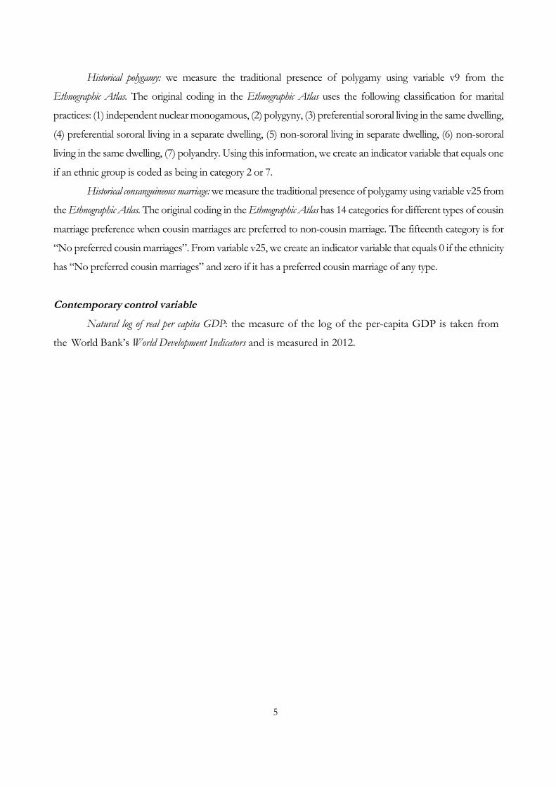
5

Historical polygamy: we measure the traditional presence of polygamy using variable v9 from the

Ethnographic Atlas. The original coding in the Ethnographic Atlas uses the following classification for marital

practices: (1) independent nuclear monogamous, (2) polygyny, (3) preferential sororal living in the same dwelling,

(4) preferential sororal living in a separate dwelling, (5) non-sororal living in separate dwelling, (6) non-sororal

living in the same dwelling, (7) polyandry. Using this information, we create an indicator variable that equals one

if an ethnic group is coded as being in category 2 or 7.

Historical consanguineous marriage: we measure the traditional presence of polygamy using variable v25 from

the Ethnographic Atlas. The original coding in the Ethnographic Atlas has 14 categories for different types of cousin

marriage preference when cousin marriages are preferred to non-cousin marriage. The fifteenth category is for

“No preferred cousin marriages”. From variable v25, we create an indicator variable that equals 0 if the ethnicity

has “No preferred cousin marriages” and zero if it has a preferred cousin marriage of any type.

Contemporary control variable

Natural log of real per capita GDP: the measure of the log of the per-capita GDP is taken from

the World Bank’s World Development Indicators and is measured in 2012.

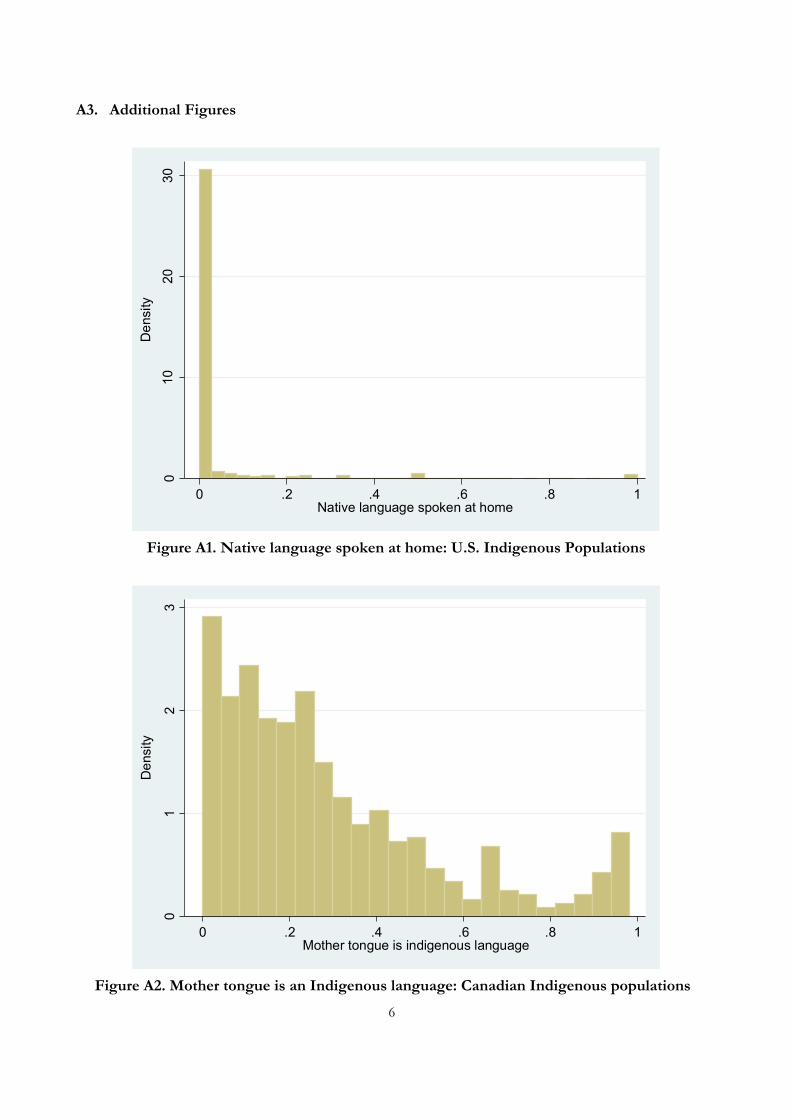
6

A3. Additional Figures

Figure A1. Native language spoken at home: U.S. Indigenous Populations

Figure A2. Mother tongue is an Indigenous language: Canadian Indigenous populations

010

2030

Den

sity

0 .2 .4 .6 .8 1Native language spoken at home

01

23

Den

sity

0 .2 .4 .6 .8 1Mother tongue is indigenous language

7

Figure A3. Indigenous language spoken at home, Canadian Indigenous populations

Figure A4. Conversational in Indigenous language, Canadian Indigenous populations

01

23

4

Den

sity

0 .2 .4 .6 .8 1Native language spoken at home

0.5

11.

52

2.5

Den

sity

0 .2 .4 .6 .8 1Convesational in indigenous language

8

A4. Additional tables

Table A1. Descriptive statistics

Variable Obs. Mean St. Dev. Variable Obs. Mean St. Dev.

Respect for tradition 75 4.521 0.549 FLFP 2012 165 53.158 15.388Traditional female part. agricult. 165 33.524 20.231

Climatic instability 75 0.252 0.108 Climatic instability 165 0.236 0.103Distance from equator 74 32.814 14.309 Log(per capita GDP) 165 9.167 1.218Economic complexity 74 6.496 1.353 Distance from the equator 165 27.437 16.851Political hierarchies 74 3.844 0.650 Economic complexity 165 6.430 1.332

Political hierarchies 165 3.489 0.907Climatic instability 75 0.252 0.110 Year ethnicity sampled 165 1.775 0.677Distance from equator 74 33.017 14.579 Polygamy 109 0.440 0.407Economic complexity 74 6.471 1.363 Traditional polygamy 109 0.702 0.409Political hierarchies 74 3.872 0.678 Consanguineous marriage 60 12.775 16.396

Traditional consanguineous marriage 60 31.204 43.151Climatic instability 75 0.253 0.113 FLFP 1970 77 32.614 17.683Distance from equator 74 33.383 14.957Economic complexity 74 6.478 1.417 FLFP 211 0.548 0.224Political hierarchies 74 3.900 0.628 Traditional female part. agricult. 211 0.392 0.238Ln(per capita GDP) 74 8.499 1.492 Climatic instability 211 0.191 0.101

Distance from the equator 211 19.834 15.139Respect for tradition 127,667 4.490 1.414 Economic complexity 211 6.351 1.509

Political hierarchies 211 3.199 1.447Climatic instability 127,667 0.271 0.117 Year ethnicity sampled 211 1.921 0.190Distance from equator 127,667 35.670 13.965Economic complexity 127,667 6.679 1.365Political hierarchies 127,667 3.008 0.854 Same country marriage 36,082 0.328 0.469

Climatic instability 36,082 0.287 0.089Climatic instability 127,685 0.265 0.118 Distance from the equator 36,082 40.163 10.268Distance from equator 127,685 35.696 13.995 Economic complexity 36,082 7.142 0.462Economic complexity 127,685 6.667 1.368 Political hierarchies 36,082 3.927 0.507Political hierarchies 127,685 3.134 0.925 Ln (per capita GDP) 36,082 9.940 0.660

Genetic distance from the US 36,082 0.476 0.577Climatic instability 126,630 0.264 0.118 Fraction of first and second gen. 36,082 0.034 0.058Distance from equator 126,630 35.695 14.065 Immigrants from same country of originEconomic complexity 126,630 6.667 1.419Political hierarchies 126,630 3.188 0.929

Women marrying men from the same country, CPS 1994-2014

With the World Ethnographic Sample Extension

With Eastern Europe and Siberia Extension

World Values Survey, Individual level sample

Baseline

Baseline

Father side

Cross-country, interactions regressionsWorld Values Survey, Country level sample

With the World Ethnographic Sample Extension

With Eastern Europe and Siberia Extension

Within-countries, interactions regressions

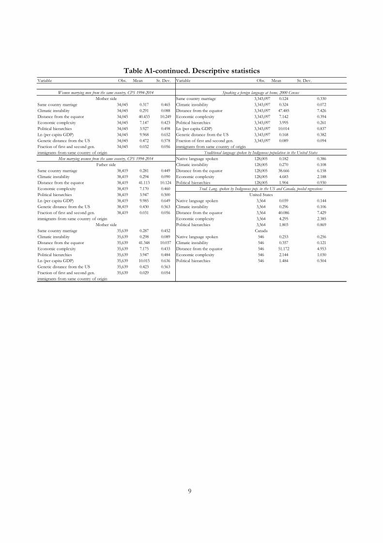
9

Table A1-continued. Descriptive statistics

Variable Obs. Mean St. Dev. Variable Obs. Mean St. Dev.

Same country marriage 3,343,097 0.124 0.330Same country marriage 34,045 0.317 0.465 Climatic instability 3,343,097 0.324 0.072Climatic instability 34,045 0.291 0.088 Distance from the equator 3,343,097 47.485 7.426Distance from the equator 34,045 40.433 10.249 Economic complexity 3,343,097 7.142 0.394Economic complexity 34,045 7.147 0.423 Political hierarchies 3,343,097 3.995 0.261Political hierarchies 34,045 3.927 0.498 Ln (per capita GDP) 3,343,097 10.014 0.837Ln (per capita GDP) 34,045 9.968 0.652 Genetic distance from the US 3,343,097 0.168 0.382Genetic distance from the US 34,045 0.472 0.578 Fraction of first and second gen. 3,343,097 0.089 0.094Fraction of first and second gen. 34,045 0.032 0.056 immigrants from same country of originimmigrants from same country of origin

Native language spoken 128,005 0.182 0.386Climatic instability 128,005 0.270 0.108

Same country marriage 38,419 0.281 0.449 Distance from the equator 128,005 38.666 6.158Climatic instability 38,419 0.294 0.090 Economic complexity 128,005 4.683 2.188Distance from the equator 38,419 41.113 10.124 Political hierarchies 128,005 1.904 0.930Economic complexity 38,419 7.170 0.460Political hierarchies 38,419 3.947 0.500Ln (per capita GDP) 38,419 9.985 0.649 Native language spoken 3,564 0.039 0.144Genetic distance from the US 38,419 0.430 0.563 Climatic instability 3,564 0.296 0.106Fraction of first and second gen. 38,419 0.031 0.056 Distance from the equator 3,564 40.086 7.429immigrants from same country of origin Economic complexity 3,564 4.295 2.385

Political hierarchies 3,564 1.803 0.869Same country marriage 35,639 0.287 0.452Climatic instability 35,639 0.298 0.089 Native language spoken 546 0.253 0.256Distance from the equator 35,639 41.348 10.037 Climatic instability 546 0.357 0.121Economic complexity 35,639 7.175 0.433 Distance from the equator 546 51.172 4.953Political hierarchies 35,639 3.947 0.484 Economic complexity 546 2.144 1.030Ln (per capita GDP) 35,639 10.015 0.636 Political hierarchies 546 1.484 0.504Genetic distance from the US 35,639 0.423 0.563Fraction of first and second gen. 35,639 0.029 0.054immigrants from same country of origin

Canada

Women marrying men from the same country, CPS 1994-2014Mother side

Men marrying women from the same country, CPS 1994-2014Father side

Mother side

Speaking a foreign language at home, 2000 Census

Traditional language spoken by Indigenous population in the United States

Trad. Lang. spoken by Indigenous pop. in the US and Canada, pooled regressionsUnited States

10

Table A2. List of ethnicities from the Word Value Survey individual-level regressions using the Ethnographic Atlas only

Ethnicity Obs. Ethnicity Obs. Ethnicity Obs. Ethnicity Obs. Ethnicity Obs.

ABKHAZ 2 CZECHS 1,917 IRANIANS 1,876 MINIANKA 10 SONINKE 30ADANGME 59 DAGARI 8 ISALA 2 MOBA 4 SOTHO 597AFAR 6 DAGOMBA 248 ISOKO 2 MOROCCANS 2,082 SPAN BASQ 13ALGERIANS 918 DARASA 6 IWA 17 MOSSI 659 SPANIARDS 15,211AMHARA 652 DIULA 156 JAPANESE 3,032 MZAB 2 SUBANUN 65AMI 1 DJUKA 96 JAVANESE 1,477 NANKANSE 6 SUMBAWANE 23ANFILLO 1 DOGON 44 JORDANIAN 2,154 NDEMBU 8 SWAZI 76ANNAMESE 969 DORSE 86 KABRE 1 NEAPOLITA 23 SYRIANS 1ARMENIANS 1,093 DUSUN 12 KALMYK 4 NEGRISEMB 7 TAGBANUA 518ASHANTI 1,866 DUTCH 19,333 KAONDE 62 NEWENGLAN 2,935 TAMIL 356ASSINI 16 EDO 1 KAREN 3 NUPE 19 TAWI-TAWI 22ATAYAL 144 EFIK 19 KARIERA 1 ORAON 33 TAZARAWA 95AYMARA 18 EGYPTIANS 4,441 KASENA 1 PAEZ 2 TELUGU 144AZJER 84 EWE 328 KASHMIRI 3 PAHARI 3 THONGA 165BABYLONIA 3,142 FRENCHCAN 542 KASONKE 40 PAIWAN 2 TIGRINYA 147BAKHTIARI 106 GA 183 KAZAK 1,867 PATHAN 228 TIV 8BAMBARA 961 GBARI 3 KERALA 279 PEDI 501 TORADJA 19BASA 2 GEORGIANS 1,419 KHASI 257 PL TONGA 218 TSAMAI 4BASARI 40 GHEG 13 KONKOMBA 3 PUNJABI 719 TSWANA 562BATAK 10 GREEKS 1,020 KONSO 6 QASHGAI 1,367 TUMBUKA 26BAULE 16 GUJARATI 391 KOREANS 3 RIFFIANS 2 TUNISIANS 1,129BEMBA 524 GURAGE 67 KUBU 3 ROMANS 794 TURKMEN 16BENGALI 317 HADIMU 12 KUNDA 28 RUSSIANS 8,295 TURKS 3,718BHIL 341 HAMYAN 42 KURD 363 RWALA 1,175 UKRAINIAN 1,167BISA 3 HAZARA 121 KUSASI 4 SANUSI 1,946 UTTARPRAD 1,152BOERS 1,008 HUNGARIAN 3,233 LEBANESE 1,161 SENOI 62 VENDA 109BOKI 2 HUTSUL 4 LIPTAKO 59 SERBS 3,054 WALLOONS 1,243BONTOK 8 IBAN 67 LOVEDU 244 SHAKO 1 XHOSA 1,001BUILSA 44 IBIBIO 6 LUIMBE 10 SHANTUNG 1,814 YAMI 11BULGARIAN 883 IBO 339 MALAYS 2,164 SHONA 1,226 YORUBA 370BYELORUSS 95 IDOMA 6 MAMPRUSI 13 SIAMESE 2,456 ZAZZAGAWA 587CAMBODIAN 136 IFUGAO 45 MANOBO 2 SIDAMO 171 ZULU 1,530CHECHEN 36 IGBIRA 4 MAORI 2 SINDHI 146CHEKIANG 6 IJAW 8 MARGI 1 SINHALESE 2 Total 127,667CHEWA 241 INCA 130 MARRI 72 SOMALI 2CHOCO 5 INGASSANA 2 MINCHINES 4,226 SONGHAI 29

11

Table A3. List of ethnicities from the Word Value Survey individual-level regressions using the Ethnographic Atlas and the Eastern Europe and Siberian extensions.

Ethnicity Obs. Ethnicity Obs. Ethnicity Obs. Ethnicity Obs. Ethnicity Obs.

Ethnicity Obs. Ethnicity Obs. Ethnicity Obs. Ethnicity Obs. Ethnicity Obs.ABKHAZ 2 CZECHS 1,909 IJAW 8 MARGI 1 SINHALESE 2ADANGME 59 DAGARI 8 INCA 130 MARRI 72 SOMALI 2AFAR 6 DAGOMBA 248 INGASSANA 2 MINCHINES 4,226 SONGHAI 29ALGERIANS 918 DARASA 6 IRANIANS 1,876 MINIANKA 10 SONINKE 30AMHARA 652 DIULA 156 ISALA 2 MOBA 4 SOTHO 597AMI 1 DJUKA 96 ISOKO 2 MOLDOVANS 12 SPAN BASQ 13ANFILLO 1 DOGON 44 IWA 17 MOROCCANS 2,082 SPANIARDS 15,211ANNAMESE 969 DORSE 86 JAPANESE 3,032 MOSSI 659 SUBANUN 65ARMENIANS 1,093 DUSUN 12 JAVANESE 1,477 MZAB 2 SUMBAWANE 23ASHANTI 1,866 DUTCH 5,563 JORDANIAN 2,154 NANKANSE 6 SWAZI 76ASSINI 16 EDO 1 KABRE 1 NDEMBU 8 SYRIANS 1ATAYAL 144 EFIK 19 KALMYK 4 NEAPOLITA 23 TAGBANUA 518AYMARA 18 EGYPTIANS 4,441 KAONDE 62 NEGRISEMB 7 TAMIL 356AZJER 84 ENGLISH 10,035 KAREN 3 NEWENGLAN 2,935 TAWI-TAWI 22BABYLONIA 3,142 ESTONIANS 1,010 KARIERA 1 NUPE 19 TAZARAWA 95BAKHTIARI 106 EWE 328 KASENA 1 ORAON 33 TELUGU 144BAMBARA 961 FRENCHCAN 542 KASHMIRI 3 PAEZ 2 THONGA 165BASA 2 GA 183 KASONKE 40 PAHARI 3 TIGRINYA 147BASARI 40 GAGAUZ 24 KAZAK 1,781 PAIWAN 2 TIV 8BATAK 10 GBARI 3 KAZAN TATAR 84 PATHAN 228 TORADJA 19BAULE 16 GEORGIANS 1,419 KERALA 279 PEDI 501 TSAMAI 4BEMBA 524 GERMANS (PRUSSIA) 3,772 KHASI 257 PL TONGA 218 TSWANA 562BENGALI 317 GHEG 13 KONKOMBA 3 PUNJABI 719 TUMBUKA 26BHIL 341 GREEKS 1,020 KONSO 6 QASHGAI 1,367 TUNISIANS 1,129BISA 3 GUJARATI 391 KOREANS 3 RIFFIANS 2 TURKMEN 16BOERS 1,008 GURAGE 67 KUBU 3 ROMANS 782 TURKS 3,694BOKI 2 HADIMU 12 KUNDA 28 RUSSIANS 8,295 UKRAINIAN 1,156BONTOK 8 HAMYAN 42 KURD 363 RWALA 1,175 UTTARPRAD 1,152BUILSA 44 HAZARA 121 KUSASI 4 SANUSI 1,946 VENDA 109BULGARIAN 883 HUNGARIAN 2,223 LEBANESE 1,161 SENOI 62 WALLOONS 1,243BYELORUSS 95 HUTSUL 4 LIPTAKO 59 SERBS 3,054 XHOSA 1,001CAMBODIAN 136 IBAN 67 LOVEDU 244 SHAKO 1 YAMI 11CHECHEN 36 IBIBIO 6 LUIMBE 10 SHANTUNG 1,814 YORUBA 370CHEKIANG 6 IBO 339 MALAYS 2,164 SHONA 1,226 ZAZZAGAWA 587CHEWA 241 IDOMA 6 MAMPRUSI 13 SIAMESE 2,456 ZULU 1,530CHOCO 5 IFUGAO 45 MANOBO 2 SIDAMO 171CHUVASH 2 IGBIRA 4 MAORI 2 SINDHI 146 Total 127,685

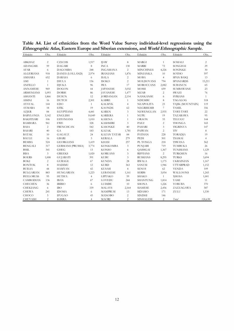
12

Table A4. List of ethnicities from the Word Value Survey individual-level regressions using the Ethnographic Atlas, Eastern Europe and Siberian extensions, and World Ethnographic Sample.

Ethnicity Obs. Ethnicity Obs. Ethnicity Obs. Ethnicity Obs. Ethnicity Obs.

ABKHAZ 2 CZECHS 1,917 IJAW 8 MARGI 1 SOMALI 2ADANGME 59 DAGARI 8 INCA 130 MARRI 72 SONGHAI 29AFAR 6 DAGOMBA 248 INGASSANA 2 MINCHINES 4,226 SONINKE 30ALGERIANS 918 DANES (LOLLAND) 2,974 IRANIANS 1,876 MINIANKA 10 SOTHO 597AMHARA 652 DARASA 6 ISALA 2 MOBA 4 SPAN BASQ 13AMI 1 DIULA 156 ISOKO 2 MOLDOVANS 794 SPANIARDS 15,211ANFILLO 1 DJUKA 96 IWA 17 MOROCCANS 2,082 SUBANUN 65ANNAMESE 969 DOGON 44 JAPANESE 3,032 MOSSI 659 SUMBAWANE 23ARMENIANS 1,093 DORSE 86 JAVANESE 1,477 MZAB 2 SWAZI 76ASHANTI 1,866 DUSUN 12 JORDANIAN 2,154 NANKANSE 6 SYRIANS 1ASSINI 16 DUTCH 2,501 KABRE 1 NDEMBU 8 TAGALOG 518ATAYAL 144 EDO 1 KALMYK 4 NEAPOLITA 23 TAJIK (MOUNTAIN) 119AYMARA 18 EFIK 19 KAONDE 62 NEGRISEMB 7 TAMIL 356AZJER 84 EGYPTIANS 4,441 KAREN 3 NEWENGLAN 2,935 TAWI-TAWI 22BABYLONIA 3,142 ENGLISH 10,049 KARIERA 1 NUPE 19 TAZARAWA 95BAKHTIARI 106 ESTONIANS 1,010 KASENA 1 ORAON 33 TELUGU 144BAMBARA 961 EWE 328 KASHMIRI 3 PAEZ 2 THONGA 165BASA 2 FRENCHCAN 542 KASONKE 40 PAHARI 3 TIGRINYA 147BASARI 40 GA 183 KAZAK 1,781 PAIWAN 2 TIV 8BATAK 10 GAGAUZ 24 KAZAN TATAR 84 PATHAN 228 TORADJA 19BAULE 16 GBARI 3 KERALA 279 PEDI 501 TSAMAI 4BEMBA 524 GEORGIANS 1,419 KHASI 257 PL TONGA 218 TSWANA 562BENGALI 317 GERMANS (PRUSSIA) 3,774 KONKOMBA 3 PUNJABI 719 TUMBUKA 26BHIL 341 GHEG 13 KONSO 6 QASHGAI 1,367 TUNISIANS 1,129BISA 3 GREEKS 1,020 KOREANS 3 RIFFIANS 2 TURKMEN 16BOERS 1,008 GUJARATI 391 KUBU 3 RUSSIANS 8,295 TURKS 3,694BOKI 2 GURAGE 67 KUNDA 28 RWALA 1,175 UKRAINIAN 1,167BONTOK 8 HADIMU 12 KURD 363 SANUSI 1,946 UTTARPRAD 1,152BUILSA 44 HAMYAN 42 KUSASI 4 SENOI 62 VENDA 109BULGARIAN 883 HUNGARIAN 1,223 LEBANESE 1,161 SERBS 3,054 WALLOONS 1,243BYELORUSS 95 HUTSUL 4 LIPTAKO 59 SHAKO 1 XHOSA 1,001CAMBODIAN 136 IBAN 67 LOVEDU 244 SHANTUNG 1,814 YAMI 11CHECHEN 36 IBIBIO 6 LUIMBE 10 SHONA 1,226 YORUBA 370CHEKIANG 6 IBO 339 MALAYS 2,164 SIAMESE 2,456 ZAZZAGAWA 587CHEWA 241 IDOMA 6 MAMPRUSI 13 SIDAMO 171 ZULU 1,530CHOCO 5 IFUGAO 45 MANOBO 2 SINDHI 146CHUVASH 2 IGBIRA 4 MAORI 2 SINHALESE 2 Total 126,630

13

Table A5. Importance of tradition using the WVS and excluding North and South America, Australia, New Zealand, and South Africa

(1) (2) (3) (4) (5) (6)

Climaticinstability -1.836*** -2.035** -1.819*** -2.074** -1.733*** -1.983**(0.582) (0.790) (0.562) (0.783) (0.524) (0.750)

Historicalcontrols:Distancefromequator 0.008 0.008 0.008

(0.006) (0.006) (0.006)Economiccomplexity -0.065* -0.061 -0.059*

(0.037) (0.037) (0.035)Politicalhierarchies -0.031 -0.040 -0.046

(0.109) (0.106) (0.121)Contemporarycontrols:Ln(percapitaGDP) -0.162*** -0.164*** -0.164***

(0.051) (0.051) (0.053)

Mean(st.dev.)ofdepvar 4.56(0.57) 4.56(0.57) 4.56(0.57) 4.56(0.57) 4.56(0.57) 4.56(0.57)Observations 63 62 63 62 63 62R-squared 0.132 0.369 0.134 0.369 0.130 0.363

AlsowiththeWorldEthnographicSample

Extension

Notes : The unit of observation is a country. The dependent variable is the average at the country levelof a measure of the self-reported importance of tradition. The mean and st. dev. of Climatic Instabilityis0.25(0.11).***,**and*indicatesignificanceatthe10,5and1%levels.

DependentVariable:ImportanceofTradition,1-6AncestralCharacteristicsMeasures

OriginalEA WithEasternEurope&SiberiaExtension

14

Table A6. The importance of tradition using the WVS: Robustness to the exclusion of potentially endogenous covariates

(1) (2) (3) (4) (5) (6)

Climaticinstability -1.626** -1.842** -1.657** -1.828** -1.600** -1.704**(0.703) (0.733) (0.703) (0.732) (0.679) (0.717)

Historicalcontrols:Distancefromequator -0.003 -0.001 -0.003 -0.001 -0.003 -0.001

(0.006) (0.005) (0.006) (0.005) (0.006) (0.005)Economiccomplexity -0.134*** -0.131*** -0.128***

(0.035) (0.035) (0.032)Politicalhierarchies 0.044 0.047 0.056

(0.115) (0.112) (0.123)

Mean(st.dev.)ofdepvar 4.52(0.55) 4.52(0.55) 4.52(0.55) 4.52(0.55) 4.52(0.55) 4.52(0.55)Observations 75 75 75 75 75 75R-squared 0.253 0.148 0.250 0.148 0.251 0.144

AncestralCharacteristicsMeasures

OriginalEA

Notes : The unit of observation is a country. The dependent variable is the average at the country level of a measure of the self-reported importance of tradition. The mean and st. dev. of Climatic Instability is 0.25 (0.11). ***, ** and * indicate significance at the 10, 5 and 1% levels.

DependentVariable:ImportanceofTradition,1-6

AlsowiththeWorldEthnographic

SampleExtension

WithEasternEurope&SiberiaExtension

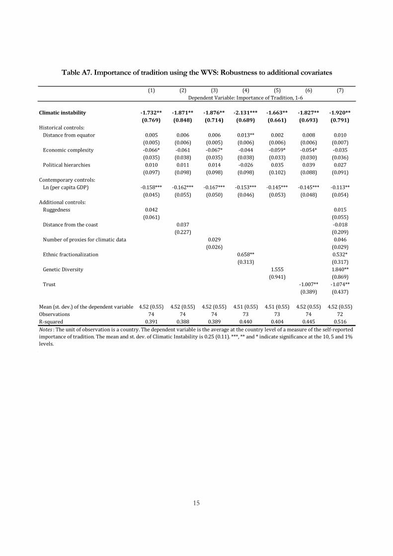
15

Table A7. Importance of tradition using the WVS: Robustness to additional covariates

(1) (2) (3) (4) (5) (6) (7)

Climaticinstability -1.732** -1.871** -1.876** -2.131*** -1.663** -1.827** -1.920**(0.769) (0.848) (0.714) (0.689) (0.661) (0.693) (0.791)

Historicalcontrols:Distancefromequator 0.005 0.006 0.006 0.013** 0.002 0.008 0.010

(0.005) (0.006) (0.005) (0.006) (0.006) (0.006) (0.007)Economiccomplexity -0.066* -0.061 -0.067* -0.044 -0.059* -0.054* -0.035

(0.035) (0.038) (0.035) (0.038) (0.033) (0.030) (0.036)Politicalhierarchies 0.010 0.011 0.014 -0.026 0.035 0.039 0.027

(0.097) (0.098) (0.098) (0.098) (0.102) (0.088) (0.091)Contemporarycontrols:Ln(percapitaGDP) -0.158*** -0.162*** -0.167*** -0.153*** -0.145*** -0.145*** -0.113**

(0.045) (0.055) (0.050) (0.046) (0.053) (0.048) (0.054)Additionalcontrols:Ruggedness 0.042 0.015

(0.061) (0.055)Distancefromthecoast 0.037 -0.018

(0.227) (0.209)Numberofproxiesforclimaticdata 0.029 0.046

(0.026) (0.029)Ethnicfractionalization 0.658** 0.532*

(0.313) (0.317)GeneticDiversity 1.555 1.840**

(0.941) (0.869)Trust -1.007** -1.074**

(0.389) (0.437)

Mean(st.dev.)ofthedependentvariable 4.52(0.55) 4.52(0.55) 4.52(0.55) 4.51(0.55) 4.51(0.55) 4.52(0.55) 4.52(0.55)Observations 74 74 74 73 73 74 72R-squared 0.391 0.388 0.389 0.440 0.404 0.445 0.516

DependentVariable:ImportanceofTradition,1-6

Notes :Theunitofobservationisacountry.Thedependentvariableistheaverageatthecountrylevelofameasureoftheself-reportedimportanceoftradition.Themeanandst.dev.ofClimaticInstabilityis0.25(0.11).***,**and*indicatesignificanceatthe10,5and1%levels.

16

Table A8. Intermarriage regressions using the CPS 1994-2014: List of countries of origin

Country Obs. Country Obs. Country Obs. Country Obs.

AFG 2 ISR 72 AFG 4 ISR 60ALB 7 ITA 3,918 ALB 6 ITA 2,885ARM 61 JAM 89 ARM 47 JAM 63ATG 1 JOR 19 ATG 2 JOR 17AUS 44 JPN 920 AUS 85 JPN 1,082AUT 382 KAZ 1 AUT 320 KEN 1BEL 86 KEN 5 BEL 113 KHM 26BGD 5 KHM 49 BGD 2 KOR 112BGR 9 KOR 69 BGR 5 LAO 86BHS 17 LAO 92 BHS 12 LBN 92BLZ 17 LBN 113 BLR 3 LKA 3BMU 8 LBR 1 BLZ 23 LTU 150BOL 13 LKA 3 BMU 20 LVA 81BRA 45 LTU 175 BOL 19 MAR 19BRB 8 LVA 82 BRA 59 MEX 7,784CAN 2,991 MAR 6 BRB 21 MKD 2CHE 139 MEX 8,431 CAN 3,391 MYS 6CHL 49 MKD 4 CHE 107 NGA 19CHN 604 MYS 6 CHL 37 NIC 100COL 177 NGA 20 CHN 528 NLD 315CPV 4 NIC 73 COL 170 NOR 284CRI 31 NLD 412 CPV 2 NZL 27CUB 558 NOR 405 CRI 28 PAK 23CYP 4 NZL 7 CUB 555 PAN 89CZE 166 PAK 31 CYP 1 PER 81DEU 2,072 PAN 58 CZE 152 PHL 947DMA 9 PER 91 DEU 2,403 POL 1,472DNK 188 PHL 1,078 DMA 6 PRI 2,104DOM 237 POL 1,715 DNK 110 PRT 288DZA 4 PRI 2,219 DOM 212 PRY 1ECU 101 PRT 395 DZA 3 ROU 93EGY 44 PRY 2 ECU 91 RUS 959ESP 258 ROU 116 EGY 38 SAU 3EST 1 RUS 1,278 ESP 193 SDN 5ETH 3 SAU 8 ETH 1 SGP 5FIN 100 SDN 29 FIN 88 SLV 334FJI 1 SGP 1 FJI 1 SVK 224

FRA 185 SLV 304 FRA 291 SWE 312GBR 1,429 SVK 269 GBR 1,855 THA 72GEO 1 SWE 377 GEO 1 TON 8GHA 3 THA 49 GHA 2 TTO 56GRC 456 TON 11 GRC 312 TUR 65GRD 6 TTO 42 GRD 1 UGA 8GTM 60 TUR 77 GTM 97 UKR 119GUY 28 UGA 13 GUY 18 URY 21HND 52 UKR 157 HND 61 VEN 30HRV 27 URY 15 HRV 16 VNM 120HTI 76 VCT 1 HTI 67 WSM 15

HUN 461 VEN 23 HUN 392 YEM 2IDN 42 VNM 111 IDN 30 ZAF 9IND 248 WSM 18 IND 207IRL 957 YEM 5 IRL 1,105IRN 85 ZAF 25 IRN 37IRQ 29 IRQ 14ISL 1 ISL 2

Total 36,082 Total 34,045

Woman marrying a husbandMother sideFather side

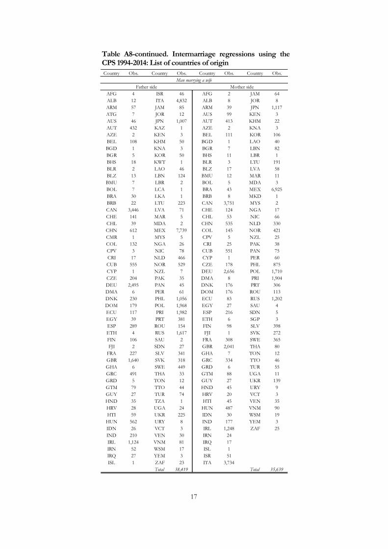
17

Table A8-continued. Intermarriage regressions using the CPS 1994-2014: List of countries of origin

Country Obs. Country Obs. Country Obs. Country Obs.

AFG 4 ISR 46 AFG 2 JAM 64ALB 12 ITA 4,832 ALB 8 JOR 8ARM 57 JAM 85 ARM 39 JPN 1,117ATG 7 JOR 12 AUS 99 KEN 3AUS 46 JPN 1,007 AUT 413 KHM 22AUT 432 KAZ 1 AZE 2 KNA 3AZE 2 KEN 3 BEL 111 KOR 106BEL 108 KHM 50 BGD 1 LAO 40BGD 1 KNA 3 BGR 7 LBN 82BGR 5 KOR 50 BHS 11 LBR 1BHS 18 KWT 1 BLR 3 LTU 191BLR 2 LAO 46 BLZ 17 LVA 58BLZ 13 LBN 124 BMU 12 MAR 11BMU 7 LBR 2 BOL 5 MDA 3BOL 7 LCA 1 BRA 43 MEX 6,925BRA 30 LKA 1 BRB 8 MKD 1BRB 22 LTU 223 CAN 3,751 MYS 2CAN 3,446 LVA 71 CHE 124 NGA 17CHE 141 MAR 5 CHL 53 NIC 66CHL 39 MDA 2 CHN 535 NLD 330CHN 612 MEX 7,739 COL 145 NOR 421CMR 1 MYS 5 CPV 5 NZL 25COL 132 NGA 26 CRI 25 PAK 38CPV 3 NIC 78 CUB 551 PAN 75CRI 17 NLD 466 CYP 1 PER 60CUB 555 NOR 529 CZE 178 PHL 875CYP 1 NZL 7 DEU 2,656 POL 1,710CZE 204 PAK 35 DMA 8 PRI 1,904DEU 2,495 PAN 45 DNK 176 PRT 306DMA 6 PER 61 DOM 176 ROU 113DNK 230 PHL 1,056 ECU 83 RUS 1,202DOM 179 POL 1,968 EGY 27 SAU 4ECU 117 PRI 1,982 ESP 216 SDN 5EGY 39 PRT 381 ETH 6 SGP 3ESP 289 ROU 154 FIN 98 SLV 398ETH 4 RUS 1,617 FJI 1 SVK 272FIN 106 SAU 2 FRA 308 SWE 365FJI 2 SDN 27 GBR 2,041 THA 80

FRA 227 SLV 341 GHA 7 TON 12GBR 1,640 SVK 318 GRC 334 TTO 46GHA 6 SWE 449 GRD 6 TUR 55GRC 491 THA 33 GTM 88 UGA 11GRD 5 TON 12 GUY 27 UKR 139GTM 79 TTO 44 HND 45 URY 9GUY 27 TUR 74 HRV 20 VCT 3HND 35 TZA 1 HTI 45 VEN 35HRV 28 UGA 24 HUN 487 VNM 90HTI 59 UKR 225 IDN 30 WSM 19

HUN 562 URY 8 IND 177 YEM 3IDN 26 VCT 3 IRL 1,248 ZAF 25IND 210 VEN 30 IRN 24IRL 1,124 VNM 81 IRQ 17IRN 52 WSM 17 ISL 1IRQ 27 YEM 3 ISR 51ISL 1 ZAF 23 ITA 3,734

Total 38,419 Total 35,639

Mother sideMan marrying a wife

Father side

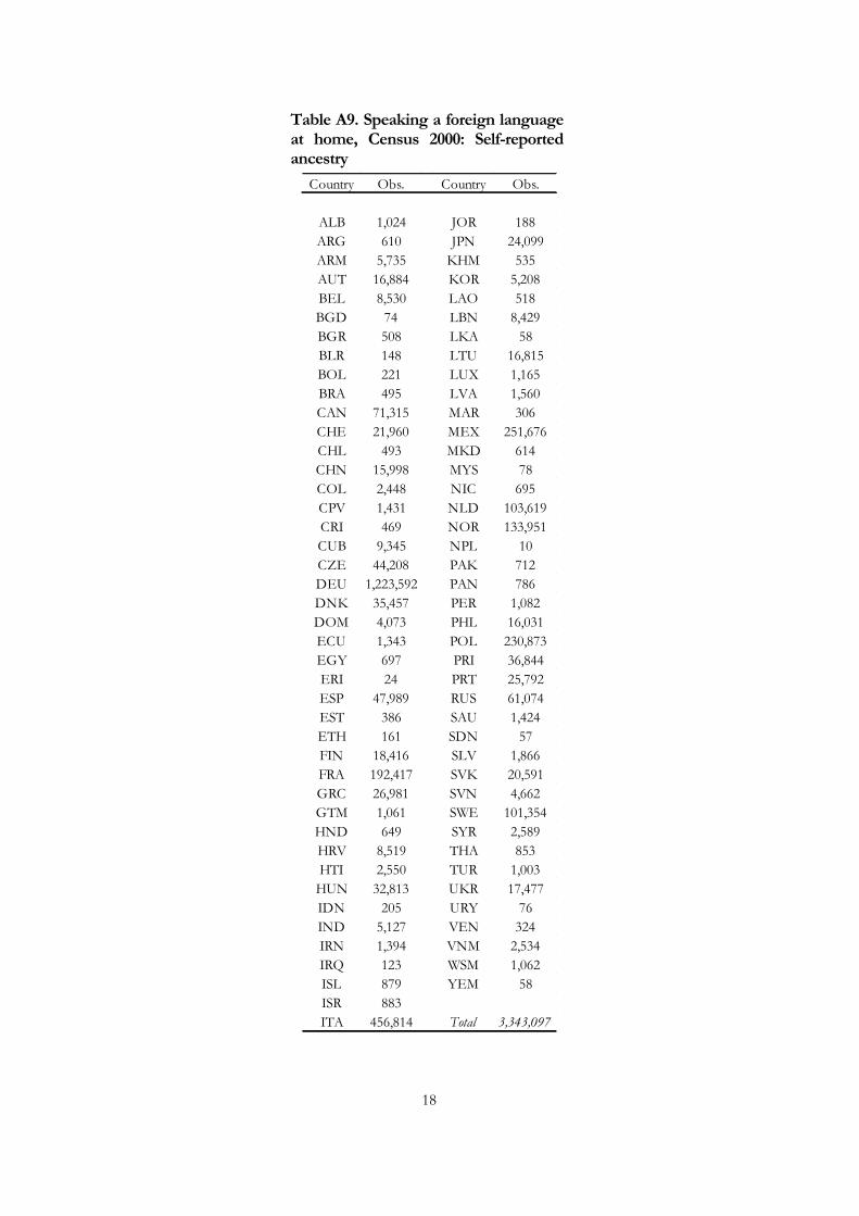
18

Table A9. Speaking a foreign language at home, Census 2000: Self-reported ancestry

Country Obs. Country Obs.

ALB 1,024 JOR 188ARG 610 JPN 24,099ARM 5,735 KHM 535AUT 16,884 KOR 5,208BEL 8,530 LAO 518BGD 74 LBN 8,429BGR 508 LKA 58BLR 148 LTU 16,815BOL 221 LUX 1,165BRA 495 LVA 1,560CAN 71,315 MAR 306CHE 21,960 MEX 251,676CHL 493 MKD 614CHN 15,998 MYS 78COL 2,448 NIC 695CPV 1,431 NLD 103,619CRI 469 NOR 133,951CUB 9,345 NPL 10CZE 44,208 PAK 712DEU 1,223,592 PAN 786DNK 35,457 PER 1,082DOM 4,073 PHL 16,031ECU 1,343 POL 230,873EGY 697 PRI 36,844ERI 24 PRT 25,792ESP 47,989 RUS 61,074EST 386 SAU 1,424ETH 161 SDN 57FIN 18,416 SLV 1,866FRA 192,417 SVK 20,591GRC 26,981 SVN 4,662GTM 1,061 SWE 101,354HND 649 SYR 2,589HRV 8,519 THA 853HTI 2,550 TUR 1,003HUN 32,813 UKR 17,477IDN 205 URY 76IND 5,127 VEN 324IRN 1,394 VNM 2,534IRQ 123 WSM 1,062ISL 879 YEM 58ISR 883ITA 456,814 Total 3,343,097

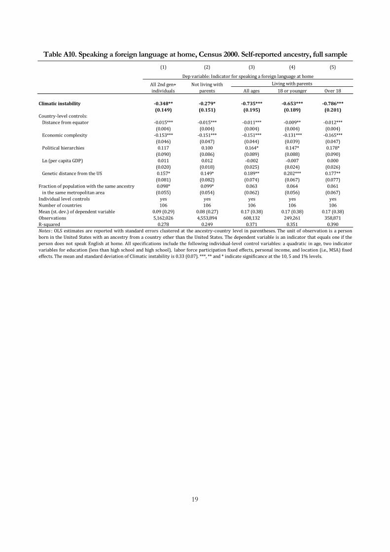
19

Table A10. Speaking a foreign language at home, Census 2000. Self-reported ancestry, full sample

(1) (2) (3) (4) (5)

Allages 18oryounger Over18

Climaticinstability -0.348** -0.279* -0.735*** -0.653*** -0.786***(0.149) (0.151) (0.195) (0.189) (0.201)

Country-levelcontrols:Distancefromequator -0.015*** -0.015*** -0.011*** -0.009** -0.012***

(0.004) (0.004) (0.004) (0.004) (0.004)Economiccomplexity -0.153*** -0.151*** -0.151*** -0.131*** -0.165***

(0.046) (0.047) (0.044) (0.039) (0.047)Politicalhierarchies 0.117 0.100 0.164* 0.147* 0.178*

(0.090) (0.086) (0.089) (0.088) (0.090)Ln(percapitaGDP) 0.011 0.012 -0.002 -0.007 0.000

(0.020) (0.018) (0.025) (0.024) (0.026)GeneticdistancefromtheUS 0.157* 0.149* 0.189** 0.202*** 0.177**

(0.081) (0.082) (0.074) (0.067) (0.077)Fractionofpopulationwiththesameancestry 0.098* 0.099* 0.063 0.064 0.061inthesamemetropolitanarea (0.055) (0.054) (0.062) (0.056) (0.067)

Individuallevelcontrols yes yes yes yes yesNumberofcountries 106 106 106 106 106Mean(st.dev.)ofdependentvariable 0.09(0.29) 0.08(0.27) 0.17(0.38) 0.17(0.38) 0.17(0.38)Observations 5,162,026 4,553,894 608,132 249,261 358,871R-squared 0.278 0.249 0.371 0.351 0.390Notes : OLS estimates are reported with standard errors clustered at the ancestry-country level in parentheses. The unit of observation is a personborn in the United States with an ancestry from a country other than the United States. The dependent variable is an indicator that equals one if theperson does not speak English at home. All specifications include the following individual-level control variables: a quadratic in age, two indicatorvariables for education (less than high school and high school), labor force participation fixed effects, personal income, and location (i.e., MSA) fixedeffects.ThemeanandstandarddeviationofClimaticinstabilityis0.33(0.07).***,**and*indicatesignificanceatthe10,5and1%levels.

Depvariable:IndicatorforspeakingaforeignlanguageathomeLivingwithparentsAll2ndgen+

individualsNotlivingwith

parents

20

Table A11. Speaking a foreign language at home, Census 2000. Self-reported ancestry, regressions collapsed at the ancestry-MSA level

(1) (2) (3) (4) (5)

Allages 18oryounger Over18

Climaticinstability -0.351* -0.257 -0.436** -0.443** -0.481***(0.198) (0.175) (0.198) (0.201) (0.170)

Country-levelcontrols:Distancefromequator -0.007*** -0.007*** -0.006*** -0.006*** -0.009***

(0.002) (0.002) (0.002) (0.002) (0.002)Economiccomplexity -0.019 -0.015 -0.038* -0.041** -0.061***

(0.017) (0.012) (0.020) (0.020) (0.020)Politicalhierarchies 0.045 0.045 0.060 0.062 0.087

(0.051) (0.046) (0.057) (0.060) (0.056)Ln(percapitaGDP) -0.026 -0.012 -0.034* -0.037** -0.011

(0.017) (0.016) (0.018) (0.018) (0.018)GeneticdistancefromtheUS 0.022 0.008 0.036 0.039 0.027

(0.043) (0.043) (0.045) (0.045) (0.047)Fractionofpopulationwiththesameancestry -0.012 0.048 -0.067 -0.070 0.018inthesamemetropolitanarea (0.317) (0.352) (0.264) (0.260) (0.241)

Numberofcountries 84 84 84 84 84Mean(st.dev.)ofdependentvariable 0.25(0.33) 0.21(0.31) 0.28(0.36) 0.28(0.36) 0.24(0.36)Observations 15,760 14,372 12,227 11,678 7,528R-squared 0.278 0.221 0.318 0.322 0.325

Depvariable:IndicatorforspeakingaforeignlanguageathomeAll2ndgen+individuals

Notlivingwithparents

Livingwithparents

Notes : OLS estimates are reported with standard errors clustered at the ancestry level in parentheses. The unit of observation is an ethnic/ancestralgroup in a location (i.e., MSA) in the United States. The dependent variable is the fraction of individuals that do not speak English at home. The meanandstandarddeviationofClimaticInstabilityis0.27(0.11).***,**and*indicatesignificanceatthe10,5and1%levels.

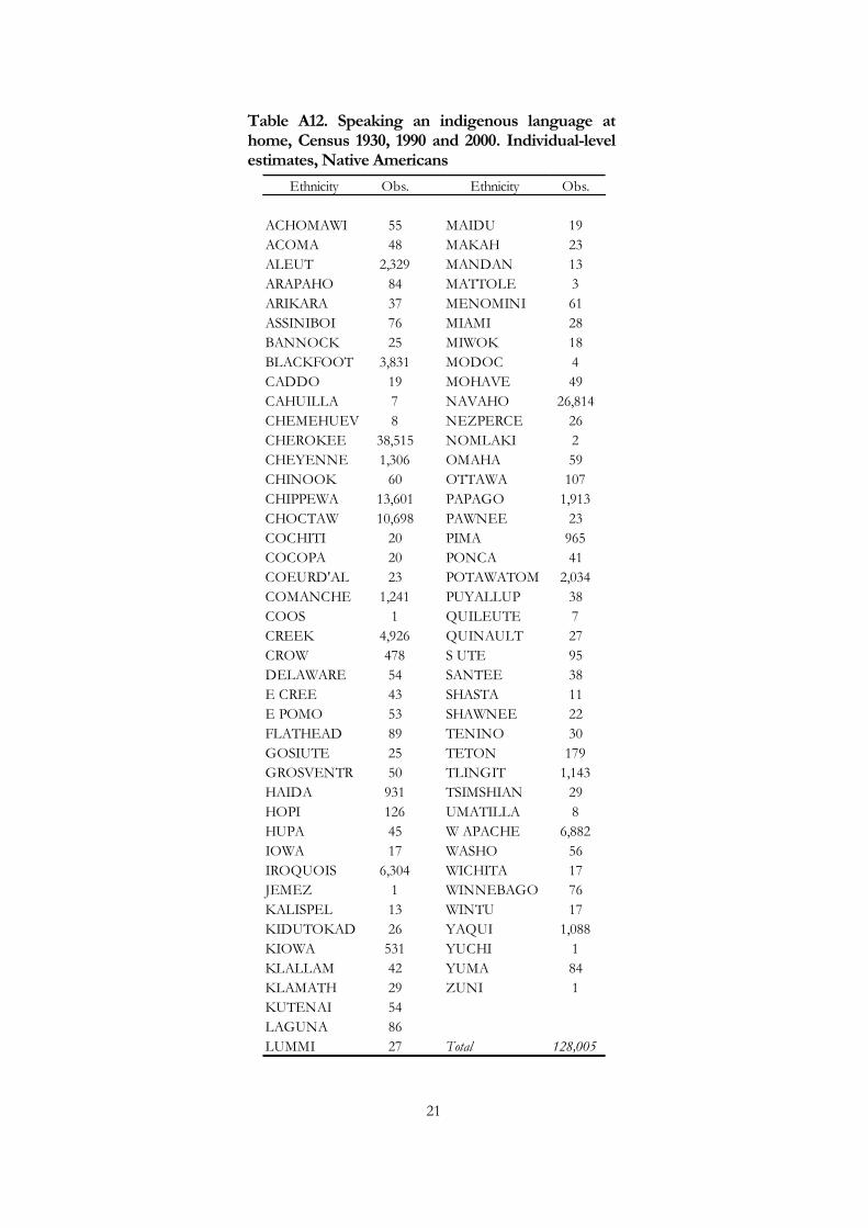
21

Table A12. Speaking an indigenous language at home, Census 1930, 1990 and 2000. Individual-level estimates, Native Americans

Ethnicity Obs. Ethnicity Obs.

ACHOMAWI 55 MAIDU 19ACOMA 48 MAKAH 23ALEUT 2,329 MANDAN 13ARAPAHO 84 MATTOLE 3ARIKARA 37 MENOMINI 61ASSINIBOI 76 MIAMI 28BANNOCK 25 MIWOK 18BLACKFOOT 3,831 MODOC 4CADDO 19 MOHAVE 49CAHUILLA 7 NAVAHO 26,814CHEMEHUEV 8 NEZPERCE 26CHEROKEE 38,515 NOMLAKI 2CHEYENNE 1,306 OMAHA 59CHINOOK 60 OTTAWA 107CHIPPEWA 13,601 PAPAGO 1,913CHOCTAW 10,698 PAWNEE 23COCHITI 20 PIMA 965COCOPA 20 PONCA 41COEURD'AL 23 POTAWATOM 2,034COMANCHE 1,241 PUYALLUP 38COOS 1 QUILEUTE 7CREEK 4,926 QUINAULT 27CROW 478 S UTE 95DELAWARE 54 SANTEE 38E CREE 43 SHASTA 11E POMO 53 SHAWNEE 22FLATHEAD 89 TENINO 30GOSIUTE 25 TETON 179GROSVENTR 50 TLINGIT 1,143HAIDA 931 TSIMSHIAN 29HOPI 126 UMATILLA 8HUPA 45 W APACHE 6,882IOWA 17 WASHO 56IROQUOIS 6,304 WICHITA 17JEMEZ 1 WINNEBAGO 76KALISPEL 13 WINTU 17KIDUTOKAD 26 YAQUI 1,088KIOWA 531 YUCHI 1KLALLAM 42 YUMA 84KLAMATH 29 ZUNI 1KUTENAI 54LAGUNA 86LUMMI 27 Total 128,005

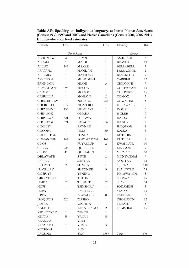
22

Table A13. Speaking an indigenous language at home Native Americans (Census 1930, 1990 and 2000) and Native Canadians (Census 2001, 2006, 2011). Ethnicity-location level estimates

Ethnicity Obs. Ethnicity Obs. Ethnicity Obs.

ACHOMAWI 2 LUMMI 1 ASSINIBOI 8ACOMA 1 MAIDU 1 BEAVER 13ALEUT 142 MAKAH 1 BELLABELL 2ARAPAHO 1 MANDAN 1 BELLACOOL 2ARIKARA 1 MATTOLE 1 BLACKFOOT 9ASSINIBOI 1 MENOMINI 1 CARRIER 22BANNOCK 1 MIAMI 3 CHILCOTIN 7BLACKFOOT 296 MIWOK 1 CHIPEWYAN 13CADDO 1 MODOC 1 CHIPPEWA 15CAHUILLA 1 MOHAVE 2 COMOX 5CHEMEHUEV 1 NAVAHO 254 COWICHAN 3CHEROKEE 517 NEZPERCE 1 DELAWARE 5CHEYENNE 133 NOMLAKI 1 DOGRIB 6CHINOOK 1 OMAHA 1 E CREE 9CHIPPEWA 321 OTTAWA 4 HAIDA 3CHOCTAW 321 PAPAGO 56 HAISLA 2COCHITI 1 PAWNEE 1 IROQUOIS 1COCOPA 1 PIMA 30 KASKA 5COEURD'AL 1 PONCA 1 KUTCHIN 6COMANCHE 147 POTAWATOM 167 KUTENAI 9COOS 1 PUYALLUP 2 KWAKIUTL 10CREEK 225 QUILEUTE 1 LILLOOET 9CROW 41 QUINAULT 1 MICMAC 60DELAWARE 1 S UTE 2 MONTAGNAI 9E CREE 1 SANTEE 1 NOOTKA 13E POMO 2 SHASTA 1 OJIBWA 118FLATHEAD 1 SHAWNEE 3 PLAINSCRE 78GOSIUTE 1 TENINO 1 POTAWATOM 3GROSVENTR 1 TETON 1 SHUSWAP 16HAIDA 67 TLINGIT 37 SLAVE 34HOPI 1 TSIMSHIAN 1 SQUAMISH 3HUPA 1 UMATILLA 1 STALO 15IOWA 1 W APACHE 305 TAHLTAN 3IROQUOIS 320 WASHO 1 THOMPSON 12JEMEZ 1 WICHITA 1 TLINGIT 3KALISPEL 1 WINNEBAGO 2 TSIMSHIAN 15KIDUTOKAD 1 WINTU 1KIOWA 38 YAQUI 68KLALLAM 1 YUCHI 1KLAMATH 1 YUMA 3KUTENAI 1 ZUNI 1LAGUNA 1 Total 3564 Total 546

United States Canada

23

Table A14. Whether the Indigenous language is spoken at home: Using the 1930 Census only

(1) (2) (3) (4) (5) (6)

All ages 18 or younger Over 18

Climatic instability -1.010* -0.862* -1.113* -1.129* -0.906* -4.955**(0.513) (0.448) (0.561) (0.567) (0.531) (2.119)

Ethnicity-level controls:Distance from equator -0.013* -0.012* -0.014* -0.015* -0.009 -0.029

(0.007) (0.007) (0.008) (0.008) (0.007) (0.074)Economic complexity -0.027* -0.022 -0.031** -0.033** -0.020 0.165

(0.014) (0.013) (0.015) (0.015) (0.016) (0.128)Political hierarchies -0.143* -0.124* -0.153* -0.153* -0.142* -0.819

(0.079) (0.071) (0.083) (0.083) (0.082) (0.626)Individual controls yes yes yes yes yes -Number of ethnic groups 82 82 78 77 66 82Number of clusters (grid cells) 39 39 39 39 39 39Mean (st. dev.) of dependent variable 0.17 (0.38) 0.17 (0.38) 0.17 (0.38) 0.17 (0.38) 0.15 (0.36) 0.02 (0.13)Observations 11,468 5,757 5,711 4,850 861 137R-squared 0.450 0.474 0.450 0.461 0.435Notes : OLS estimates are reported with standard errors clustered at the level of the climatic grid cell in parentheses, in columns 1-5. Poisson estimatesare reported with standard errors clustered at the grid cell level in column 6. The unit of observation is a person who identifies him/herself as a NativeAmerican in columns 1-5 and an Indigenous ethnic group living in a given location, in column 6. The dependent variable is an indicator that equals oneif the person speaks an indigenous (i.e., Native American) language at home in columns 1-5, and the fraction of poeple speaking an Indigenouslanguage at home in column 6. All specification in columns 1-5 include the following covariates: a quadratic in age, a gender indicator, employmentstatus fixed effects, an indicator for being married, metropolitan area fixed effects, an indicator for whether the individual has any education. Themean (and standard deviation) of Climatic instability is 0.27 (0.11).

Dep var: Fraction speaking an Indigenous

language at home

Dep variable: Indicator for speaking an Indigenous language at home

All individualsNot living with

parents

Living with parents