
Empirical finance - EconStor
279
econstor Make Your Publications Visible. A Service of zbw Leibniz-Informationszentrum Wirtschaft Leibniz Information Centre for Economics Hamori, Shigeyuki (Ed.) Book — Published Version Empirical finance Provided in Cooperation with: MDPI – Multidisciplinary Digital Publishing Institute, Basel Suggested Citation: Hamori, Shigeyuki (Ed.) (2019) : Empirical finance, ISBN 978-3-03897-707-0, MDPI, Basel, http://dx.doi.org/10.3390/books978-3-03897-707-0 This Version is available at: http://hdl.handle.net/10419/203848 Standard-Nutzungsbedingungen: Die Dokumente auf EconStor dürfen zu eigenen wissenschaftlichen Zwecken und zum Privatgebrauch gespeichert und kopiert werden. Sie dürfen die Dokumente nicht für öffentliche oder kommerzielle Zwecke vervielfältigen, öffentlich ausstellen, öffentlich zugänglich machen, vertreiben oder anderweitig nutzen. Sofern die Verfasser die Dokumente unter Open-Content-Lizenzen (insbesondere CC-Lizenzen) zur Verfügung gestellt haben sollten, gelten abweichend von diesen Nutzungsbedingungen die in der dort genannten Lizenz gewährten Nutzungsrechte. Terms of use: Documents in EconStor may be saved and copied for your personal and scholarly purposes. You are not to copy documents for public or commercial purposes, to exhibit the documents publicly, to make them publicly available on the internet, or to distribute or otherwise use the documents in public. If the documents have been made available under an Open Content Licence (especially Creative Commons Licences), you may exercise further usage rights as specified in the indicated licence. https://creativecommons.org/licenses/by/4.0/ www.econstor.eu
-
Upload
khangminh22 -
Category
Documents
-
view
2 -
download
0
Transcript of Empirical finance - EconStor

econstorMake Your Publications Visible.
A Service of
zbwLeibniz-InformationszentrumWirtschaftLeibniz Information Centrefor Economics
Hamori, Shigeyuki (Ed.)
Book — Published Version
Empirical finance
Provided in Cooperation with:MDPI – Multidisciplinary Digital Publishing Institute, Basel
Suggested Citation: Hamori, Shigeyuki (Ed.) (2019) : Empirical finance, ISBN978-3-03897-707-0, MDPI, Basel,http://dx.doi.org/10.3390/books978-3-03897-707-0
This Version is available at:http://hdl.handle.net/10419/203848
Standard-Nutzungsbedingungen:
Die Dokumente auf EconStor dürfen zu eigenen wissenschaftlichenZwecken und zum Privatgebrauch gespeichert und kopiert werden.
Sie dürfen die Dokumente nicht für öffentliche oder kommerzielleZwecke vervielfältigen, öffentlich ausstellen, öffentlich zugänglichmachen, vertreiben oder anderweitig nutzen.
Sofern die Verfasser die Dokumente unter Open-Content-Lizenzen(insbesondere CC-Lizenzen) zur Verfügung gestellt haben sollten,gelten abweichend von diesen Nutzungsbedingungen die in der dortgenannten Lizenz gewährten Nutzungsrechte.
Terms of use:
Documents in EconStor may be saved and copied for yourpersonal and scholarly purposes.
You are not to copy documents for public or commercialpurposes, to exhibit the documents publicly, to make thempublicly available on the internet, or to distribute or otherwiseuse the documents in public.
If the documents have been made available under an OpenContent Licence (especially Creative Commons Licences), youmay exercise further usage rights as specified in the indicatedlicence.
https://creativecommons.org/licenses/by/4.0/
www.econstor.eu

Empirical FinanceShigeyuki Hamori
www.mdpi.com/journal/jrfm
Edited by
Printed Edition of the Special Issue Published in Journal of Risk and Financial Management
Journal of

Empirical Finance


Empirical Finance
Special Issue Editor
Shigeyuki Hamori
MDPI • Basel • Beijing • Wuhan • Barcelona • Belgrade

Special Issue Editor
Shigeyuki Hamori
Kobe University
Japan
Editorial Office
MDPI
St. Alban-Anlage 66
4052 Basel, Switzerland
This is a reprint of articles from the Special Issue published online in the open access journal
Journal of Risk and Financial Management (ISSN 1911-8074) from 2018 to 2019 (available at: https://
www.mdpi.com/journal/jrfm/special issues/empirical)
For citation purposes, cite each article independently as indicated on the article page online and as
indicated below:
LastName, A.A.; LastName, B.B.; LastName, C.C. Article Title. Journal Name Year, Article Number,
Page Range.
ISBN 978-3-03897-706-3 (Pbk)
ISBN 978-3-03897-707-0 (PDF)
c© 2019 by the authors. Articles in this book are Open Access and distributed under the Creative
Commons Attribution (CC BY) license, which allows users to download, copy and build upon
published articles, as long as the author and publisher are properly credited, which ensures maximum
dissemination and a wider impact of our publications.
The book as a whole is distributed by MDPI under the terms and conditions of the Creative Commons
license CC BY-NC-ND.

Contents
About the Special Issue Editor . . . . . . . . . . . . . . . . . . . . . . . . . . . . . . . . . . . . . . vii
Zhouhao Wang, Enda Liu, Hiroki Sakaji, Tomoki Ito, Kiyoshi Izumi, Kota Tsubouchi and
Tatsuo Yamashita
Estimation of Cross-Lingual News Similarities Using Text-Mining MethodsReprinted from: J. Risk Financ. Manag. 2018, 11, 8, doi:10.3390/jrfm11010008 . . . . . . . . . . . . 1
Eiji Ogawa and Makoto Muto
What Determines Utility of International Currencies?Reprinted from: J. Risk Financ. Manag. 2019, 12, 10, doi:10.3390/jrfm12010010 . . . . . . . . . . . 14
Zhaojie Luo, Xiaojing Cai, Katsuyuki Tanaka, Tetsuya Takiguchi, Takuji Kinkyo and
Shigeyuki Hamori
Can We Forecast Daily Oil Futures Prices? Experimental Evidence from Convolutional NeuralNetworksReprinted from: J. Risk Financ. Manag. 2019, 12, 9, doi:10.3390/jrfm12010009 . . . . . . . . . . . . 45
Dimitrios Vezeris, Themistoklis Kyrgos and Christos Schinas
Take Profit and Stop Loss Trading Strategies Comparison in Combination with an MACDTrading SystemReprinted from: J. Risk Financ. Manag. 2018, 11, 56, doi:10.3390/jrfm11030056 . . . . . . . . . . . 58
Lei Xu, Takuji Kinkyo and Shigeyuki Hamori
Predicting Currency Crises: A Novel Approach Combining Random Forests and WaveletTransformReprinted from: J. Risk Financ. Manag. 2018, 11, 86, doi:10.3390/jrfm11040086 . . . . . . . . . . . 81
Aneta Ptak-Chmielewska
Predicting Micro-Enterprise Failures Using Data Mining TechniquesReprinted from: J. Risk Financ. Manag. 2019, 12, 30, doi:10.3390/jrfm12010030 . . . . . . . . . . . 92
Shigeyuki Hamori, Minami Kawai, Takahiro Kume, Yuji Murakami and Chikara Watanabe
Ensemble Learning or Deep Learning? Application to Default Risk AnalysisReprinted from: J. Risk Financ. Manag. 2018, 11, 12, doi:10.3390/jrfm11010012 . . . . . . . . . . . 109
Brian F. Tivnan, David Slater, James R. Thompson, Tobin A. Bergen-Hill, Carl D. Burke,
Shaun M. Brady, Matthew T. K. Koehler, Matthew T. McMahon, Brendan F. Tivnan and
Jason G. Veneman
Price Discovery and the Accuracy of Consolidated Data Feeds in the U.S. Equity MarketsReprinted from: J. Risk Financ. Manag. 2018, 11, 73, doi:10.3390/jrfm11040073 . . . . . . . . . . . 123
Tadahiro Nakajima
Expectations for Statistical Arbitrage in Energy Futures MarketsReprinted from: J. Risk Financ. Manag. 2019, 12, 14, doi:10.3390/jrfm12010014 . . . . . . . . . . . 140
Takashi Miyazaki
Clarifying the Response of Gold Return to Financial Indicators: An Empirical ComparativeAnalysis Using Ordinary Least Squares, Robust and Quantile RegressionsReprinted from: J. Risk Financ. Manag. 2019, 12, 33, doi:10.3390/jrfm12010033 . . . . . . . . . . . 152
v

Yuki Toyoshima
Testing for Causality-In-Mean and Variance between the UK Housing and Stock MarketsReprinted from: J. Risk Financ. Manag. 2018, 11, 21, doi:10.3390/jrfm11020021 . . . . . . . . . . . 170
Guizhou Liu, Xiao-Jing Cai and Shigeyuki Hamori
Modeling the Dependence Structure of Share Prices among Three Chinese City BanksReprinted from: J. Risk Financ. Manag. 2018, 11, 57, doi:10.3390/jrfm11040057 . . . . . . . . . . . 180
Xie He, Xiao-Jing Cai and Shigeyuki Hamori
Bank Credit and Housing Prices in China: Evidence from a TVP-VAR Model with StochasticVolatilityReprinted from: J. Risk Financ. Manag. 2018, 11, 90, doi:10.3390/jrfm11040090 . . . . . . . . . . . 198
Joanna Lizinska and Leszek Czapiewski
Is Window-Dressing around Going Public Beneficial? Evidence from PolandReprinted from: J. Risk Financ. Manag. 2019, 12, 18, doi:10.3390/jrfm12010018 . . . . . . . . . . . 214
Su-Lien Lu and Ying-Hui Li
Effect of Corporate Governance on Institutional Investors’ Preferences: An EmpiricalInvestigation in TaiwanReprinted from: J. Risk Financ. Manag. 2019, 12, 32, doi:10.3390/jrfm12010032 . . . . . . . . . . . 230
Vinh Nguyen Thi Thuy and Duong Trinh Thi Thuy
The Impact of Exchange Rate Volatility on Exports in Vietnam: A Bounds Testing ApproachReprinted from: J. Risk Financ. Manag. 2019, 12, 6, doi:10.3390/jrfm12010006 . . . . . . . . . . . . 251
Haifeng Xu
Book Review for “Credit Default Swap Markets in the Global Economy” by Go Tamakoshi andShigeyuki Hamori. Routledge: Oxford, UK, 2018; ISBN: 9781138244726Reprinted from: J. Risk Financ. Manag. 2018, 11, 68, doi:10.3390/jrfm11040068 . . . . . . . . . . . 265
vi

About the Special Issue Editor
Shigeyuki Hamori is a Professor of Economics, Graduate School of Economics, Kobe University,
Japan. He holds a Ph.D. in Economics from Duke University, the United States. He is a Distinguished
Fellow, International Engineering and Technology Institute (DFIETI), and Honorary Chair Professor,
Asia University, Taiwan. His main research interests are applied time series analysis, empirical
finance, data science, and international finance. He has published approximately 200 articles
in international peer-reviewed journals, and he is presently a member of the editorial boards of
International Review of Financial Analysis, Singapore Economic Review, AGING AND HEALTH, Advances
in Decision Sciences, Journal of Risk and Financial Management, Annals of Financial Economics, Journal
of Management Information and Decision Sciences, International Economics and Finance Journal, Journal of
Reviews on Global Economics, and Accounting and Finance Research. He is also the Vice President of the
International Research Institute for Economics and Management (IRIEM).
vii

Journal of
Risk and FinancialManagement
Article
Estimation of Cross-Lingual News Similarities UsingText-Mining Methods
Zhouhao Wang 1,*, Enda Liu 1, Hiroki Sakaji 1,*, Tomoki Ito 1, Kiyoshi Izumi 1,*,
Kota Tsubouchi 2 and Tatsuo Yamashita 2
1 Izumi lab, Department of System Innovation, Graduate School of Engineering, The University of Tokyo,Hongo 7-3-1, Bunkyo-ku, Tokyo 113-0033, Japan; [email protected] (E.L.); [email protected] (T.I.)
2 Yahoo! Japan Research, Kioicho 1-3, Chiyoda-ku, Tokyo 102-8282, Japan; [email protected] (K.T.);[email protected] (T.Y.)
* Correspondence: [email protected] (Z.W.); [email protected] (H.S.);[email protected] (K.I.); Tel.: +81-03-5841-6993 (K.I.)
Received: 31 December 2017; Accepted: 25 January 2018; Published: 31 January 2018
Abstract: In this research, two estimation algorithms for extracting cross-lingual news pairs based onmachine learning from financial news articles have been proposed. Every second, innumerable textdata, including all kinds news, reports, messages, reviews, comments, and tweets are generated on theInternet, and these are written not only in English but also in other languages such as Chinese, Japanese,French, etc. By taking advantage of multi-lingual text resources provided by Thomson Reuters News,we developed two estimation algorithms for extracting cross-lingual news pairs from multilingual textresources. In our first method, we propose a novel structure that uses the word information and themachine learning method effectively in this task. Simultaneously, we developed a bidirectional LongShort-Term Memory (LSTM) based method to calculate cross-lingual semantic text similarity for long textand short text, respectively. Thus, when an important news article is published, users can read similarnews articles that are written in their native language using our method.
Keywords: text similarity; text mining; machine learning; SVM; neural network; LSTM
1. Introduction
Text similarity, as its name suggests, refers to how similar a given text query is to others.We normally tend to consider texts based mainly on their semantic characteristics, that is, how close(i.e., similar) their meanings are. Here, the text could be in the form of character level, word level,sentence level, paragraph level, or even longer, document level. In this paper, we mainly discuss textthat is in the form of sentences (i.e., short text) and documents (i.e., long text).
The objective of this research could be summarized in three key points. The fundamentalobjective is to develop algorithms for estimation of semantic similarity for the given two pieces of textwritten in different languages, applicable for both long text and short text, by taking advantage theuntapped vast suppository of text resources from Thomson Reuters economics news reports. Secondly,as a practical application and a verification of our model, we are aiming at developing a cross-lingualrecommendation system and test benchmark, which could provide several of the most-related (forexample, 10 results) pieces of Japanese or English text when given an English (or Japanese) article.Thirdly, we excavate cross-lingual resources from the enormous database of Thomson Reuters Newsand build an effective cross-lingual system by taking advantage of this un-developed treasure.
2. Related Work and Theories
Regardless of the length of the text, most of the state-of-the-art methods have recently beenimplemented based on word embedding methods and thus we discuss this in detail in a separate
JRFM 2018, 11, 8; doi:10.3390/jrfm11010008 www.mdpi.com/journal/jrfm1

JRFM 2018, 11, 8
section. To solve semantic text similarity problems, one of the most typical and inspiring methods isSiamese LSTM structure, which is considered as both a basis and a competitive baseline of this research.
2.1. Embedding Techniques for Words and Documents
Word embedding technique, also known as distributed word representation, is one of the mostbasic concepts and applications prevalent nowadays. Word embedding could be further extendedto be performed on documents. The embedding techniques capture both the semantic and syntacticinformation and convert them into meaningful feature vectors which help to train accurate models fornatural language processing (NLP) tasks (Tang et al. 2014).
Word embedding can be implemented for both monolingual and multilingual tasks. There areseveral successful papers working on the monolingual word embedding such as the continuous bagof words models and skip-gram models (Mikolov et al. 2013), monolingual document embeddingsuch as doc2vec (Le and Mikolov 2014), cross-lingual word embedding (Zou et al. 2013), as well ascross-lingual document embedding models such as Bilingual Bag-of-Words without Word Alignments(BilBOWA) (Gouws et al. 2015). Through embedding model, each word, phrase or document would beconverted into a fixed length vector representation, where the similarity between two words, phrases,or documents could be derived by calculating the cosine distance of their vector representations.Methods are distinctly different for the text data with different length when solving the text similarityproblem (Le and Mikolov 2014). With respect to the length of the text, a textual similarity task could befurther categorized into two sub-tasks. Prevalent methods for cross-lingual document (i.e., long text)similarity could be categorized into four aspects (Rupnik et al. 2016), Dictionary-based approaches(Kudo et al. 2004), Probabilistic topic model based approaches (Taghva et al. 2005), Matrix factorizationbased approaches (Lo et al. 2014), and Monolingual approaches.
2.2. Text Similarities Using Siamese LSTM
Neural network-based Siamese recurrent architectures have recently proved to be one of the mosteffective ways for learning semantic text similarity on the sentence level. Mueller, in his work, implementsa Siamese recurrent structure called Manhattan LSTM (MaLSTM) (Mueller and Thyagarajan 2016),which is practically used as the estimation of relativeness (i.e., similarity) when given any two sentencesin English. This structure uses Long Short-Term Memory (LSTM) (Hochreiter and Schmidhuber 1997) andhas a state-of-the-art performance on both semantic relatednesses scoring task and entailment classificationusing the SICK database, one of the NLP challenges provided by SemEval (Agirre et al. 2016). This modelcould identify how two sentences are similar to each other by trying to “understand” their true meaning ona deeper aspect, like the sentence pairs “He is smart” and “A truly wise man” as the figure demonstrates.They have no common words with different lengths, but they are indeed highly relevant to each otherin terms of their implications, which a human cannot recognize without more consideration and logicalanalysis, suggesting the difficulty of this challenge.
In our work, we developed a new recurrent structure inspired by MaLSTM, by modifying theSiamese (i.e., symmetric) LSTM modules to “unbalanced” ones, and adding a full-connect neuralnetwork layer following the output of LSTM modules, which is more flexible and effective than a textsimilarity task.
3. Methods for Extracting Cross-Lingual News Pairs
In this section, we will introduce all fundamental and necessary methods applied in our research.There are mainly three aspects to be elaborated, including methods we applied regarding thefoundation of natural language processing, such as word embedding and TF-IDF. We explainedtwo applied methods, one of which is the classical methods learning SVM (Support Vector Machine).The other one is the neural network method, LSTM(Long-Short Term Memory).
2

JRFM 2018, 11, 8
3.1. Distribution Representation
The most traditional and naive way to consider words as features is to treat words as discretesymbols or numbers. This results in a discrete representation of each word and hinders theestablishment of relations among these features. In contrast, vector space models consider (embedded)words in a continuous vector space, in which words with similar meanings are separated by smalldistances. There are two main categories for continuous word embedding: count-based (suchas latent semantic analysis) models and predictive-based methods (such as neural probabilisticlanguage models). The count-based models focus on the co-occurrence of the considered wordand its neighboring words, whereas the predictive-based models predict a word based on its neighborsusing embedding vectors Baroni et al. (2014). In this research, we implement a predictive-basedmodel that is known as word2vec; it is based on the skip-gram or continuous bag-of-words modelMikolov et al. (2013).
We train each word from the training text sequence w1, w2, w3, ..., wT to maximize theobjective function
1T
T
∑t=1
∑−c≤j≤c,j �=0
log p(wt+j|wt) (1)
wherein c is the so-called “window size,” which determines how much context information isto be considered for each of the training words. More specifically, we define p(wt+j|wt) using asoftmax function:
p(wO|wI) =exp(vwO
TvwI )
∑Ww=1 exp(vwTvwI )
(2)
wherein W is the size of the vocabulary (i.e., the number of disparate words to be considered), and v isthe vector representations for either the word w, the input word wI , or the output word wO.
However, the calculation of Equation (2) is impractical because the computational cost forcalculating the gradient of log p(wt+j|wt) is proportional to W, which consists of as many as 105 to 107
terms. In practical terms, to train the model (i.e., optimize the cost function) in a more computationallyefficient manner, we use Noise Contrastive Estimation for approximation during training, as describedin Mikolov et al. (2013).
Finally, vector representations with fixed dimension (e.g., 200) can be extracted from the trainedmodel. These word vectors have some outstanding attributes. Because we train our model for eachword using its neighboring words, and words with similar meaning usually tend to have similarcontext, we can calculate the similarity among words using the cosine distance.
3.2. Term Frequency-Inversed Document Frequency (TF-IDF)
TF-IDF is one of the classical weighting models for words, which uses text representations. It iswidely used in the natural language processing domain wherein it is commonly applied for weightingwords or document features, such as in one-hot bag-of-words representation. The term frequencystands for the number of times a considered word occurs in a specific document, while the documentfrequency is the number of documents in the corpus that include the word. The inverse documentfrequency term for a specific word can be expressed as
id f = logN
1 + d f(3)
wherein N is the total number of documents in the corpus. Combining these two concepts, the TF-IDFweight is the product of the TF and the IDF. This scheme loses semantic information for words; thus,it usually cannot achieve satisfactory performance. However, it measures the weights and importanceof each word inside documents and among other documents according to a reasonable definition.In this study, we apply TF-IDF to weight words during document embedding.
3

JRFM 2018, 11, 8
3.3. TF-IDF Weighting for Word Vectors
Although there are several ways to form vector representations for documents (i.e., documentembedding), we have experimentally discovered that the most effective strategy is to use the TF-IDFweighted sum of the word vectors that are present in each document as features. First, we calculatetwo TF-IDF weighting models, namely TF-IDFjp and TF-IDFen, for each word from English trainingdocuments and Japanese training documents. Second, for each Japanese document, the weighted sumdocument representation can be derived as
Ji =Ni
∑m=0
ti,m · wi,m (4)
wherein Ni refers to the number of words in this Japanese document (i.e., Japanese document i),and ti,m stands for the Japanese TF-IDF weight for the m-th word in document i with respect to theconsidered word. The final term wi,m is the word vector of the m-th word in document i, that is,the vector representation for this considered word.
We apply the same weighting scheme to the English documents. The vector representation forEnglish document i can be expressed as
Ei =Ni
∑m=0
ti,m · wi,m (5)
wherein all the definitions of the above variables are the same as those in the Japanese processing case,except the texts are in English.
3.4. Feature Engineering
The selection of features is possibly the most significant and tricky step, in particular, for classicalmachine learning algorithms such as SVM. This is called “feature engineering” because sometimes thechoice of features can greatly affect the results. Fortunately, as one of the most exciting results in thisresearch, we discover that satisfactory results can be generated using the joint cross-lingual documentvector that is based on TF-IDF weighted word2vec as a training feature for the SVM model. Althoughboth SVM and TF-IDF weighted word vectors are common in the text mining domain, to the bestof our knowledge, this is the first time that the effectiveness of using joint cross-lingual text featurevectors as input for SVM on the cross-lingual text similarity problem has been proved.
More specifically, for the vector representation of a Japanese document Ji and an English documentEj, the joint features are defined by
fi,j = (Ji, Ej) (6)
Via feature engineering, we prepare our training datasets S, which contain a subset S1 of instancesfor which the similarity scores are all equal to 1:
S1 = {(f1,1, 1), ..., (fN,N, 1)} (7)
and another subset S0 of instances for which the similarity scores are all equal to 0:
S0 = {(f1,o, 0), ...(fQ,P, 0)} (8)
wherein N is the total number of cross-lingual training pairs with similarity of 1 (i.e., similar pairs)for training and o is an arbitrary number that belongs to (1, N) and is not equal to 1, such that f1,o isthe set of dissimilar pairs with similarity of 0 (i.e., the pairs are totally unrelated). Moreover, note thatQ, P ∈ (1, N) and Q �= N.
4
JRFM 2018, 11, 8
Hence, our final training data S isS = S1 ∪ S0 (9)
3.5. The SVM-Based Method
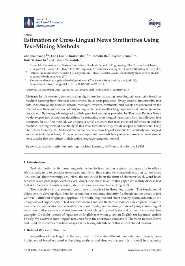
SVM is one of the most popular methods for solving both classification and regression tasks.It was originally purposed in 1990s and gradually proved to be effective in many fields includingNatural language processing (NLP), pattern recognition and so on (Burges 1998; Malakasiotis andAndroutsopoulos 2007; Béchara et al. 2015). TF-IDF and SVM are useful for tasks in the fieldof natural language processing. Therefore, we employ TF-IDF and SVM in our method as coretechnologies. Additionally, we propose a novel structure that uses TF-IDF and SVM effectively for thistask. An overview of the structure is illustrated in Figure 1.
The system mainly contains three processing models. As our our training datasets, S onlycontains the data with label 0 or 1, the classification training objective of SVM is very similar toclassification using Triplet Loss, which is proved to be quite effective in embedding and classificationtasks (Schroff et al. 2015). The training procedures normally include the following steps:
1. Use the cross-lingual training data in the form of pre-trained word vectors as input, which isdiscussed in detail in Section 3.1.
2. Weight the word vectors for each of language models using TF-IDF, as introduced inSubsections 3.2 and 3.3.
3. Train the proposed model using SVM with Platt’s probability estimation for the connectedcross-lingual document features, each of which are the naive join of two weighted word sumvectors in English and Japanese. This is explained in Section 3.4.
Figure 1. Illustration of our SVM-based method.
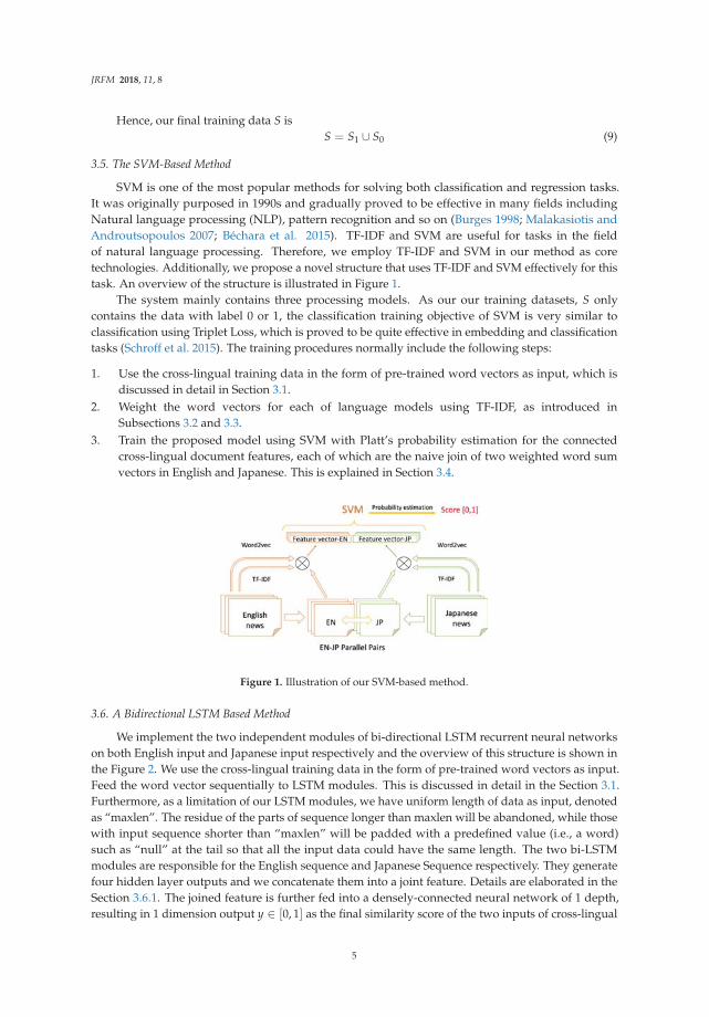
3.6. A Bidirectional LSTM Based Method
We implement the two independent modules of bi-directional LSTM recurrent neural networkson both English input and Japanese input respectively and the overview of this structure is shown inthe Figure 2. We use the cross-lingual training data in the form of pre-trained word vectors as input.Feed the word vector sequentially to LSTM modules. This is discussed in detail in the Section 3.1.Furthermore, as a limitation of our LSTM modules, we have uniform length of data as input, denotedas “maxlen”. The residue of the parts of sequence longer than maxlen will be abandoned, while thosewith input sequence shorter than “maxlen” will be padded with a predefined value (i.e., a word)such as “null” at the tail so that all the input data could have the same length. The two bi-LSTMmodules are responsible for the English sequence and Japanese Sequence respectively. They generatefour hidden layer outputs and we concatenate them into a joint feature. Details are elaborated in theSection 3.6.1. The joined feature is further fed into a densely-connected neural network of 1 depth,resulting in 1 dimension output y ∈ [0, 1] as the final similarity score of the two inputs of cross-lingual
5
JRFM 2018, 11, 8
data, by means of regression. In general, the LSTM-based model pays more attention to the orderinformation of the input sequence, which might significantly determine the real meaning of a sentencewritten in natural languages.
3.6.1. The Bi-LSTM Layer
In this research, we take advantage of bi-LSTM (bi-directional long short-term memory),to enhance the ordinary RNN performance considering both forward and backward informationand solve the problem of the long-term dependencies. The updates rules of LSTM for each sequentialinput x1, x2, ..., xt, ..., xT could be express as:
it = sigmoid(Wixt + Uiht−1 + bi) (10)
ft = sigmoid(Wf xt + Uf ht−1 + b f ) (11)
ct = tanh(Wcxt + Ucht−1 + bc) (12)
ct = it � ct + ft � ct−1 (13)
ot = sigmoid(Woxt + Uoht−1 + bo) (14)
ht = ot � tanh(ct) (15)
where ht−1 is the hidden layer value of the previous states and the sigmoid and tanh functions in theabove equations are also used as activation functions:
sigmoid(x) =1
1 + exp(−x)(16)
tanh(x) =2
1 + exp(−2x)− 1 (17)
The weights (i.e., parameters) we need to train include Wi, Wf , Wc, Wo, Ui, Uf , Uc, Uo and bias vectorsbi, b f , bc, bo. A more thorough exposition of the LSTM model and its variants is provided by(Graves 2012) and (Greff et al. 2017). In this layer, we use the cross-lingual training data in theform of pre-trained word vectors as input, which is discussed in detail in Section 3.1. There arefour LSTM modules, constructing two bi-LSTM structures, where we only consider the final output(i.e., final value of the hidden layer) of each LSTM module: LSTM-a read Japanese text in a forwarddirection. The value of a hidden layer is denoted as h
(a)i where i is the i-th input of the sequence,
while LSTM-b read backwards, denoted as h(b)i . Symmetrically, LSTM-c and LSTM-d are used to read
English text, denoted as h(c)i and h
(d)i . As the results, we obtain four feature vectors derived from
hidden layer values of the four LSTM modules, keeping all necessary information regarding to thecross-lingual inputs. We then merge these four features by concatenating them directly:
xi,j = (h(a)L , h
(b)L , h
(c)L , h
(d)L ) (18)
where i and j refer to the document number of the input text for Japanese and English respectively,and vector h
(a,b,c,d)L refers to the final status (i.e., the value) of the hidden layers of the LSTM module
after feeding the last (or the first, if backwards) word.
6

JRFM 2018, 11, 8
Figure 2. Illustration of the LSTM-based method.
3.6.2. Dense Layer
We use the most basic component of the basic full-dense Neural Network layer as the top layer.The function of this layer could be expressed as:
yi,j = f (wTxi,j + b) (19)
Here, the function f is also known as “activation” function, b is the one dimensional bias for the neuralnetwork and w is the weight (i.e., the parameters to be trained) of the neural network. In this project,we mainly apply the softplus Nair and Hinton (2010) function as the activation function in the dense layer:
f (x) = ln[1 + exp(x)] (20)
As for the optimization, although we are handling a classification problem, based on the experimentalresults, we find that, instead of using ordinary cross-entropy cost, it performs better if we use Quadraticcost (i.e., mean square error) as the cost function, which could be described as:
C =N
∑v=1
(ytrue,v − ypred,v)2 (21)
where N is the total number of the training data, while ytrue,v and ypred,v refer to the true similarity andthe predicted similarity, respectively. In practice, the stochastic gradient descent (SGD) is implementedby means of the back-propagation scheme. After computing the outputs and errors based on the costfunction J, which is usually equal to the negative log of the maximum likelihood function, we updateparameters by the gradient descent method, expressed as:
w ← w − ε∇w J(w) (22)
where ε is known as “learning rate”, defining the update speed of the hyper-parameters w. However,the training process might fail due to either improper initialization regarding weights or the improperlearning rate value set. Practically, based on the results of the experiments, the best performance isachieved by applying the Adam optimizer Kingma and Ba (2014) to perform the parameter updates.
4. Experiments and Results
4.1. Evaluation Methods
We mainly use two categories of the evaluations, TOP-N benchmark based on ranks, and traditionalcriteria for classification such as precision, recall as well as the F1-value. As the applications of this
7
JRFM 2018, 11, 8
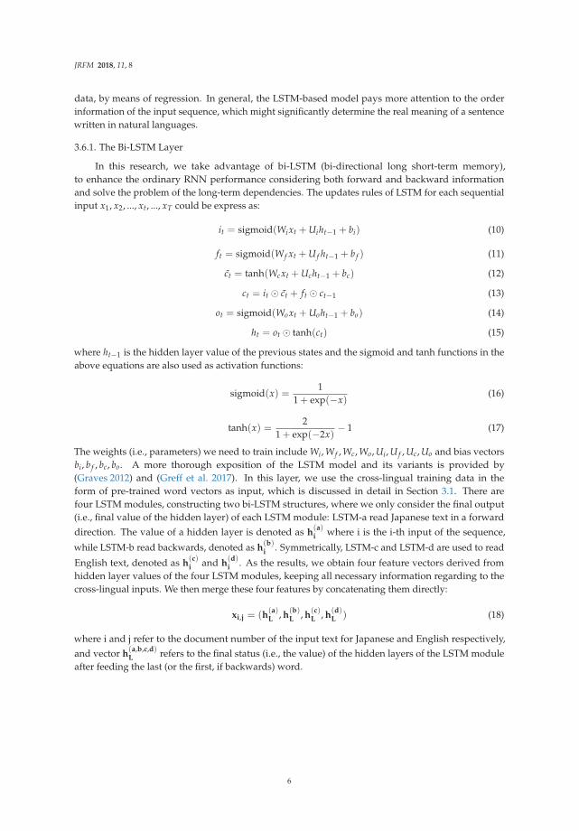
project aim to suggest several cross-lingual (For instance, English) alternative news stories to the users,when the user provides a Japanese article as a query, we make the system pick up 1, 5 and 10 of the mostsimilar Japanese alternatives during the evaluation process. The Figure 3 illustrates the relationship andevaluation procedures for ranks, TOP-N index.For a given Japanese text (i.e., the query) Jx, calculatethe similarity score between Jx and all English text of test data sets (E1, E2, ..., Ex, ..., EM) to derive alist of scores Lx = (Sx,1, Sx,2, ..., Sx,x, ..., Sx,M) , where the corner mark M is the total number of Englishdocuments to be considered, and Ex is the true similar article with a similarity score of 1. Then sort thislist in the order from large to small and find out the rank (i.e., position, index) of the score Sx,x insidethis sorted list noted as Rx, the rank for the query document Jx. Repeat this process recursively for NJapanese articles (J1, J2, ..., JN), result in a list of ranks R = (R1, R2, ..., RN) regarding the collectionsof Jx. Then we take the number of query documents with ranks smaller than N as TOP-N. In otherwords, TOP-1 refers to the number of query documents with rank equal to 1 and TOP-5 refers to thenumber of a query with rank equal to or smaller than 5.
Figure 3. Illustration of an evaluation procedures using ranks and TOP-N index.
4.2. Baseline: Siamese LSTM with Google-Translation
Siamese LSTM is one of the deep learning-based models with the art-of-state performance on thesemantic text similarity problems. In this research, we make this model a baseline by extending thismodel from a monolingual domain to a cross-lingual domain with the help of the Google Translationservices. We first translate all Japanese text into the English version on both test and training data byusing the google translate service1 Then we implement the Siamese LSTM model as described in theoriginal paper for Siamese LSTM Mueller and Thyagarajan (2016) with the help of the open sourcecode on the Github2 To illustrate this baseline method regarding a two cross-lingual input, we firsttranslate the Japanese input into an English sentence using Google Translation service. Then, we canconsider the cross-lingual task as monolingual one so that we can apply the Siamese LSTM model fortraining as a baseline.
4.3. Datasets and Pre-Processing
Thomson Reuters news3 is a worldwide news agency providing worldwide news in multiplelanguages. Most of the reports are originally written in English and translated and edited into otherlanguages including Chinese, Japanese, etc. These multi-lingual texts are expected to be highly potentialresources for tasks related to the multi-lingual natural languages processing. In this research, we use60,000 news articles in 2014 from Thomson Reuters News related to the economics. For the preprocessingof text, we convert raw data to normalized data, which could be further used to train word2vec models
1 Google Translation Web API could be accessed from https://github.com/aditya1503/Siamese-LSTM.2 The open source code for Siamese LSTM can be accessed from https://github.com/aditya1503/Siamese-LSTM.3 Official websites of Thomson Reuters: http://www.reuters.com/.
8
JRFM 2018, 11, 8
for both English and Japanese text, respectively. We train the Japanese word2vec model and Englishword2vec model separately using news articles with the same contents in 2014. In our experiment, weuse the model of a Continuous Bag of Words (CBOW), with 200 fixed dimensions of word embedding.Other parameters are set using the default value used in the Gensim package4.
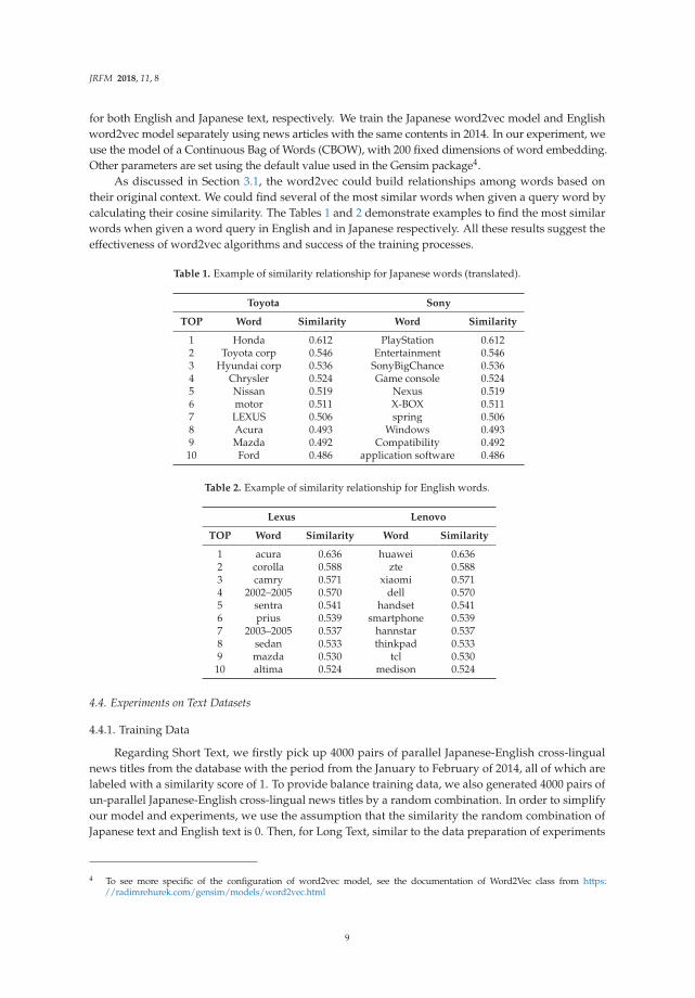
As discussed in Section 3.1, the word2vec could build relationships among words based ontheir original context. We could find several of the most similar words when given a query word bycalculating their cosine similarity. The Tables 1 and 2 demonstrate examples to find the most similarwords when given a word query in English and in Japanese respectively. All these results suggest theeffectiveness of word2vec algorithms and success of the training processes.
Table 1. Example of similarity relationship for Japanese words (translated).
Toyota Sony
TOP Word Similarity Word Similarity
1 Honda 0.612 PlayStation 0.6122 Toyota corp 0.546 Entertainment 0.5463 Hyundai corp 0.536 SonyBigChance 0.5364 Chrysler 0.524 Game console 0.5245 Nissan 0.519 Nexus 0.5196 motor 0.511 X-BOX 0.5117 LEXUS 0.506 spring 0.5068 Acura 0.493 Windows 0.4939 Mazda 0.492 Compatibility 0.492
10 Ford 0.486 application software 0.486
Table 2. Example of similarity relationship for English words.
Lexus Lenovo
TOP Word Similarity Word Similarity
1 acura 0.636 huawei 0.6362 corolla 0.588 zte 0.5883 camry 0.571 xiaomi 0.5714 2002–2005 0.570 dell 0.5705 sentra 0.541 handset 0.5416 prius 0.539 smartphone 0.5397 2003–2005 0.537 hannstar 0.5378 sedan 0.533 thinkpad 0.5339 mazda 0.530 tcl 0.53010 altima 0.524 medison 0.524
4.4. Experiments on Text Datasets
4.4.1. Training Data
Regarding Short Text, we firstly pick up 4000 pairs of parallel Japanese-English cross-lingualnews titles from the database with the period from the January to February of 2014, all of which arelabeled with a similarity score of 1. To provide balance training data, we also generated 4000 pairs ofun-parallel Japanese-English cross-lingual news titles by a random combination. In order to simplifyour model and experiments, we use the assumption that the similarity the random combination ofJapanese text and English text is 0. Then, for Long Text, similar to the data preparation of experiments
4 To see more specific of the configuration of word2vec model, see the documentation of Word2Vec class from https://radimrehurek.com/gensim/models/word2vec.html
9
JRFM 2018, 11, 8
for short text introduced, we prepare 4000 parallel (i.e., similarity = 1) Japanese-English news articlesand 4000 un-parallel (i.e., similarity = 0) ones for training data through random combination.
4.4.2. Test Data
For Short Text, in order to evaluate our model more comprehensively, we have prepared two setsof independent test data. TEST-1S contains 1000 pairs of parallel Japanese-English news titles, selectedand split from the same period of training data, from January 2014 to the middle of February in 2014.Similarly, TEST-2S contains title pairs with time stamps of December 2014. For Long Text, similar tothe case of short test evaluation, we have prepared two sets of independent test data. For training data,we prepared a similar dataset as for the short text experiments. TEST-1L and TEST-2L contain 1000pairs of parallel Japanese-English long news articles respectively.
4.4.3. Ranks and TOP-N
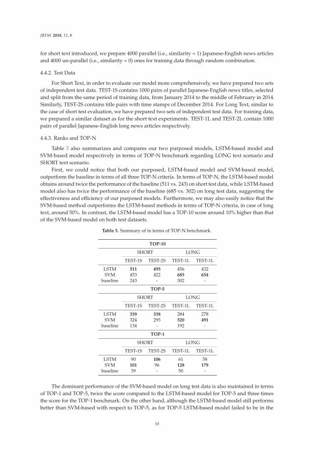
Table 3 also summarizes and compares our two purposed models, LSTM-based model andSVM-based model respectively in terms of TOP-N benchmark regarding LONG text scenario andSHORT text scenario.
First, we could notice that both our purposed, LSTM-based model and SVM-based model,outperform the baseline in terms of all three TOP-N criteria. In terms of TOP-N, the LSTM-based modelobtains around twice the performance of the baseline (511 vs. 243) on short test data, while LSTM-basedmodel also has twice the performance of the baseline (685 vs. 302) on long test data, suggesting theeffectiveness and efficiency of our purposed models. Furthermore, we may also easily notice that theSVM-based method outperforms the LSTM-based methods in terms of TOP-N criteria, in case of longtext, around 50%. In contrast, the LSTM-based model has a TOP-10 score around 10% higher than thatof the SVM-based model on both test datasets.
Table 3. Summary of in terms of TOP-N benchmark.
TOP-10
SHORT LONG
TEST-1S TEST-2S TEST-1L TEST-1L
LSTM 511 495 456 432SVM 453 422 685 654
baseline 243 - 302 -
TOP-5
SHORT LONG
TEST-1S TEST-2S TEST-1L TEST-1L
LSTM 339 338 284 278SVM 324 295 520 491
baseline 134 - 192 -
TOP-1
SHORT LONG
TEST-1S TEST-2S TEST-1L TEST-1L
LSTM 90 106 61 58SVM 101 96 128 179
baseline 39 - 50 -
The dominant performance of the SVM-based model on long test data is also maintained in termsof TOP-1 and TOP-5, twice the score compared to the LSTM-based model for TOP-5 and three timesthe score for the TOP-1 benchmark. On the other hand, although the LSTM-based model still performsbetter than SVM-based with respect to TOP-5, as for TOP-5 LSTM-based model failed to be in the
10

JRFM 2018, 11, 8
lead anymore. We are going to discuss these results and propose possible hypotheses and provideexplanations in Section 5. The performance of successful recommendation numbers from our bi-LSTMbased model is twice that of the baseline.
5. Discussion
5.1. Comparison of the Baseline and the LSTM-Based Model
The performance of the LSTM-based model is twice that of the baseline, even though they areboth based on LSTM structures. The differences, which are also the innovations for this purposedmethod, compared to the baseline, include the using of bi-LSTM, independent LSTM modules as wellas using the fully connected neural network as the final layer.
First, the baseline method is able to calculate the similarity of two sentences, no matter whetherthere are different types of word arrangement for the two inputs, or if there are different words usedreferring to the same meaning, which proves the effectiveness of the encoding (i.e., embedding) abilityfor the input text. However, the baseline model has the “Siamese LSTM structure”, which means,in other words, that the two LSTM instances always share the same parameters during the training.This might be effective for a monolingual case, but not good enough on the cross-lingual case. Thus,the LSTM instances used in our purposed model are all independently holding their own uniqueparameters. In addition, the bi-directional structure also helps to encode the feature of each inputtext more comprehensively. Finally, instead of using cosine similarity as the final layer in the baselinemethod, we used the fully connected neural network as output, making the output layer adjust (i.e.,train) its parameters so as to learn precise patterns from the features generated by LSTMs. We believethese three modifications improve the final results for our LSTM-based model.
5.2. Comparison of the LSTM-Based Model and SVM-Based Model
The experiments above leave us with an interesting question about why the LSTM-based modeland SVM-based model perform differently regarding the length of the target text we train and test.We explain this question in two aspects.
5.2.1. From the Point of View of the SVM-Based Model
Since the SVM-based methods use the TF-IDF weighting which is a classical and an effectivemethod for NLP fields to extract the most important and representative features for each of documentcomprehensively, it could accurately identify the most significant feature, a few key words, from a verylong and complex article containing hundreds of words, in both Japanese and English, and then finallyfeed them into the SVM classifier to get the similarity estimation universally. However, due to theattributes of TF-IDF algorithms, the shorter the length of each document is, the less information theTF-IDF could extract. This is because if there are fewer words in one document, every word could beeither unique or common regarding other documents, resulting in the failure of TF-IDF. This might bethe reason why SVM-based model performs well on long datasets but this performance becomes pooron shorter data sets.
5.2.2. From the Point of View of the LSTM-Based Model
On the other hand, the LSTM is good at understanding sentences by means of grasping the orderinformation of each words, since for any natural languages, not only words themselves but also theorder of words, to some extent, define the true meaning of a sentence. Especially for short text, a slightchange of the order could alter the meaning of the sentences significantly and thus the LSTM-basedmodel outperformed the LSTM model by around 10% on short datasets. However, LSTM is not good atextracting the key idea of longer documents since, although LSTM solves the problem of memorizinglong text (i.e., solve of the problem of gradient vanishing and gradient explosion), it could tell the
11

JRFM 2018, 11, 8
importance of each word as TF-IDF does. That might be the possible reason why it fails to performeffectively on a long text.
6. Conclusions
We developed a bi-LSTM-based model to calculate cross-lingual similarities given a pair of Englishand Japanese articles. Instead of using a translation module or a dictionary to translate from one toanother language, our model has outstanding performance with short text. Furthermore, we modifiedand implemented a popular Siamese LSTM model as the baseline and we found both of our modelsoutperform the baseline. For practical testing, we defined the concept of “TOP-N” and “ranks” totest the overall performance of the model, with visualized results. We also make a comparative studybased on the results of the experiments that bi-LSTM based obtains better performance on short textdata such as news titles and alert messages, which are on average shorter than 20 words, in contrast tonormal news articles with more than 200 words on average. As the results show, both models obtainedsatisfactory performance with over half of the test documents of 1000 holding ranks lower than 10(i.e., TOP-10). As a high-performance cross-lingual news calculating system, we expect that it couldachieve optimal performance by taking advantage of both models to form a complete system.
Supplementary Materials: The following are available online at www.mdpi.com/1911-8074/11/1/8/s1.
Acknowledgments: Thanks three anonymous reviewers from JRFM for reviewing our paper, and providingvaluable instructions to revise our paper.
Author Contributions: Zhouhao Wang, Enda Liu and Hiroki Sakaji conceived and designed the experiments.Enda Liu performed the experiments. Zhouhao Wang and Enda Liu analyzed the data. Tomoki Ito, Kiyoshi Izumi,Kota Tsubouchi and Tatsuo Yamashita contributed materials. Zhouhao Wang, Hiroki Sakaji and Kiyoshi Izumiwrote the paper.
Conflicts of Interest: The authors declare no conflict of interest.
References
Agirrea, Eneko, Carmen Baneab, Daniel Cerd, Mona Diabe, Aitor Gonzalez-Agirrea, Rada Mihalceab,German Rigaua, and Janyce Wiebe. 2016. Semeval-2016 task 1: Semantic textual similarity, monolingualand cross-lingual evaluation. Paper presented at the SemEval-2016, San Diego, CA, USA, June 16–17,pp. 497–511.
Baroni, Marco, Georgiana Dinu, and German Kruszewski. 2014. Don’t count, predict! a systematic comparison ofcontext-counting vs. context-predicting semantic vectors. Paper presented at the 52nd Annual Meeting ofthe Association for Computational Linguistics, Baltimore, MD, USA, June 23–25, pp. 238–47.
Béchara, Hanna, Hernani Costa, Shiva Taslimipoor, Rohit Gupta, Constantin Orasan, Gloria Corpas Pastor,and Ruslan Mitkov. 2015. Miniexperts: An svm approach for measuring semantic textual similarity. Paperpresented at the 9th International Workshop on Semantic Evaluation (SemEval 2015), Denver, CO, USA,June 4–5, pp. 96–101.
Burges, Christopher J. C. 1998. A tutorial on support vector machines for pattern recognition. Data Mining andKnowledge Discovery 2: 121–67.
Gouws, Stephan, Yoshua Bengio, and Greg Corrado. 2015. Bilbowa: Fast bilingual distributed representationswithout word alignments. Paper presented at the 32nd International Conference on Machine Learning(ICML-15), Lille, France, July 7, pp. 748–56.
Graves, Alex. 2012. Supervised Sequence Labelling with Recurrent Neural Networks. Berlin and Heidelberg: Springer,vol. 385.
Greff, Klaus, Rupesh K. Srivastava, Jan Koutník, Bas R. Steunebrink, and Jürgen Schmidhuber. 2017. Lstm:A search space odyssey. IEEE Transactions on Neural Networks and Learning Systems 28: 2222–32.
Hochreiter, Sepp, and Jürgen Schmidhuber. 1997. Long short-term memory. Neural Computation 9: 1735–80.Kingma, Diederik P., and Jimmy Ba. 2014. Adam: A Method for Stochastic Optimization. Available online:
https://arxiv.org/abs/1412.6980 (accessed on 16 August 2017).
12

JRFM 2018, 11, 8
Kudo, Taku, Kaoru Yamamoto, and Yuji Matsumoto. 2004. Applying conditional random fields to japanesemorphological analysis. Paper presented at the 2004 Conference on Empirical Methods in Natural LanguageProcessing, Barcelona, Spain, July 25, vol. 4, pp. 230–37.
Le, Quoc, and Tomas Mikolov. 2014. Distributed representations of sentences and documents. Paper presented atthe 31st International Conference on Machine Learning (ICML-14), Beijing, China, June 23, pp. 1188–96.
Lo, Chi-kiu, Meriem Beloucif, Markus Saers, and Dekai Wu. 2014. Xmeant: Better semantic mt evaluation withoutreference translations. Paper presented at the 52nd Annual Meeting of the Association for ComputationalLinguistics (Volume 2: Short Papers), Baltimore, MD, USA, June 23–25, vol. 2, pp. 765–71.
Malakasiotis, Prodromos, and Ion Androutsopoulos. 2007. Learning textual entailment using svms andstring similarity measures. Paper presented at the ACL-PASCAL Workshop on Textual Entailment andParaphrasing, Prague, Czech Republic, June 28–29. Stroudsburg: Association for Computational Linguistics,pp. 42–47.
Mikolov, Tomas, Ilya Sutskever, Kai Chen, Greg Corrado, and Jeffrey Dean. 2013. Distributed representationsof words and phrases and their compositionality. Paper presented at the 26th International Conference onNeural Information Processing Systems, Lake Tahoe, NV, USA, December 5–10, pp. 3111–19.
Mueller, Jonas, and Aditya Thyagarajan. 2016. Siamese recurrent architectures for learning sentence similarity.Paper presented at the 30th AAAI Conference on Artificial Intelligence (AAAI 2016), Phoenix, AZ, USA,February 16, pp. 2786–92.
Nair, Vinod, and Geoffrey E. Hinton. 2010. Rectified linear units improve restricted boltzmann machines. Paperpresented at the 27th International Conference on Machine Learning (ICML-10), Haifa, Israel, June 21–24,pp. 807–14.
Rupnik, Jan, Andrej Muhic, Gregor Leban, Blaz Fortuna, and Marko Grobelnik. 2016. News acrosslanguages-cross-lingual document similarity and event tracking. Journal of Artificial Intelligence Research 55:283–316.
Schroff, Florian, Dmitry Kalenichenko, and James Philbin. 2015. Facenet: A unified embedding for face recognitionand clustering. Paper presented at Proceedings of the IEEE Conference on Computer Vision and PatternRecognition, Boston, MA, USA, June 7–12, pp. 815–23.
Taghva, Kazem, Rania Elkhoury, and Jeffrey Coombs. 2005. Arabic stemming without a root dictionary. Paperpresented at International Conference on Information Technology: Coding and Computing, 2005 (ITCC2005), Las Vegas, NV, USA, April 4–6, vol. 1, pp. 152–157.
Tang, Duyu, Furu Wei, Nan Yang, Ming Zhou, Ting Liu, and Bing Qin. 2014. Learning sentiment-specificword embedding for twitter sentiment classification. Paper presented at the 52nd Annual Meeting of theAssociation for Computational Linguistics, Baltimore, MD, USA, June 23–25, pp. 1555–65.
Zou, Will Y., Richard Socher, Daniel Cer, and Christopher D. Manning. 2013. Bilingual word embeddings forphrase-based machine translation. Paper presented at the 2013 Conference on Empirical Methods in NaturalLanguage Processing, Seattle, WA, USA, October 19, pp. 1393–98.
c© 2018 by the authors. Licensee MDPI, Basel, Switzerland. This article is an open accessarticle distributed under the terms and conditions of the Creative Commons Attribution(CC BY) license (http://creativecommons.org/licenses/by/4.0/).
13

Journal of
Risk and FinancialManagement
Article
What Determines Utility of International Currencies?
Eiji Ogawa 1,2,* and Makoto Muto 1
1 Graduate School of Business Administration, Hitotsubashi University, Tokyo 186-8601, Japan;[email protected]
2 Research Institute of Economy, Trade and Industry (RIETI), Tokyo 100-8901, Japan* Correspondence: [email protected]
Received: 7 December 2018; Accepted: 3 January 2019; Published: 8 January 2019
Abstract: In previous studies, we estimated a time series of coefficients on five international currencies(the US dollar, the euro, the Japanese yen, the British pound, and the Swiss franc) in a utility function.We call the coefficients utilities of international currencies. The time series show that the utilityof the US dollar as an international currency has remained in the first position in the changinginternational monetary system despite of the fact that the euro was created as a single commoncurrency for European countries. On one hand, the utility of the Japanese yen has been declining asan international currency. In this paper, we investigate what determines the utility of internationalcurrencies. We use a dynamic panel data model to analyze the issue with Generalized Methodof Moments (GMM). Specifically, liquidity shortage in terms of an international currency meansthat it is inconvenient for economic agents to use the relevant currency for international economictransactions. In other words, liquidity shortages might reduce the utility of an international currency.In this analysis we focus on liquidity premium which represents a liquidity shortage in terms ofan international currency. Our empirical results showed not only inertia in terms of change butalso the impact of a liquidity shortage in an international currency on the utility of the relevantinternational currency.
Keywords: utility of international currency; inertia; liquidity risk premium; US dollar; Japanese yen
1. Introduction
The United States (US) dollar had been as a rule a key currency in the Bretton Woods internationalmonetary system. The monetary authority of the United States fixed the US dollar to gold while themonetary authorities of other countries fixed their home currencies to the US dollar under the BrettonWoods system. It could keep stability of exchange rates among the currencies in the world economy.However, the Bretton Woods system was collapsed in 1971 because the monetary authority of theUnited States could not keep a value of the US dollar against gold to stop convertibility of the USdollar to gold. Afterwards, a position of the US dollar as a key currency has been still kept in thecurrent international monetary system even though we have no longer the rule under which we haveto use the US dollar as a key currency. The phenomenon is called as inertia of a key currency.
Given that a key currency is chosen for economic reasons which include costs and benefits of aninternational currency, comparison in costs and benefits of international currencies determines a keycurrency in the current international monetary policy. Also, inertia of a key currency should be relatedwith inertia of costs and/or benefits of holding an international currency. The costs of holding aninternational currency are related with its depreciation that caused by inflation in the relevant country.On one hand, the benefits of holding an international currency are caused by utility of holding it.
In a Sidrauski (1967)-type of money-in-the-utility model (Calvo 1981, 1985; Obstfeld 1981; Blanchardand Fischer 1989), real balances of money as well as consumption are supposed as explanatory variablesin a utility function. We can use the money-in-the-utility model to analyze costs and benefits of holding
JRFM 2019, 12, 10; doi:10.3390/jrfm12010010 www.mdpi.com/journal/jrfm14

JRFM 2019, 12, 10
international currencies. Ogawa and Muto (2017a, 2017b) used expected inflation rates and Bankfor International Settlements (BIS) data on total of domestic currency denominated debt and foreigncurrency denominated debt of the euro currency market to estimate time series of coefficients on fiveinternational currencies (the US dollar, the euro, the Japanese yen, the British pound, and the Swissfranc) in a utility function. We call the coefficients utility of an international currency. The time seriesshow that utility of the US dollar as an international currency has kept at the first position even thoughthe euro was introduced into some of the European Union (EU) states while it increased utility ofthe euro as an international currency. On one hand, utility of the Japanese yen has been decliningas an international currency. Since 1973, although the US dollar is downward trend, it has kept thekey currency in the changing international monetary system. This is probably because the US dollarhas reduced the store of value function but maintained the medium of exchange function. Utility ofthe international currency means relative contribution of holding an international currency throughsuch functions of international currency. Therefore, we can estimate relative position of internationalcurrency from a value of utility of the international currency.
In this paper, we have an objective to investigate what determines utility of the internationalcurrencies. We use a dynamic panel data model to analyze the issue with Generalized Method ofMoments (GMM). Specifically, liquidity shortage in terms of an international currency means that it isinconvenient for economic agents to use the relevant currency for international economic transactions.In other words, the liquidity shortage might reduce utility of an international currency. In this analysiswe focus on liquidity premium which represents liquidity shortage in terms of an internationalcurrency. We make empirical analysis of whether liquidity risk premium in an international currencyaffects utility of the relevant international currency. For example, if the currency authority aims tointernationalize its home currency, results of this analysis will be useful for which variables shouldbe focused.
We obtain the following results from the empirical study. Firstly, change in utility of the currencyin the previous period has significantly a positive effect on the change of utility of the currency in thecurrent period. This suggests that utility of the currency tends to fluctuate in the same direction asthe change in the previous period. For example, if the utility of the currency declines, we assumedthat the currency is less likely to be used than in the previous period, which will continue in the nextperiod. Secondly, the change of liquidity risk premium has a significantly negative effect on the changeof utility of the currency. This suggests that liquidity shortage reduce the utility of the internationalcurrency. Thirdly, the change of capital flow share has significantly a positive effect on the change ofutility of the currency. This suggests that changes in economic scale, specifically capital flow, affect theutility of the international currency.
In the next section, we describe related literatures. In the third section, we explain our theoreticalmodel in terms of utility of an international currency. In the fourth section, we explain empirical modelfor analyzing determinants of utility of an international currency. In the fifth section, we explain dataused for the analysis and calculation method. In the sixth section, we discuss hypothesis of estimatedcoefficients and influence of each variable on utility of an international currency. In the seventh section,we show results of dynamic panel analysis. Finally, we conclude our empirical analysis.
2. Related Literature
Krugman (1984) adopted three functions of money as a medium of exchange, a unit of account,and a store of value to consider six roles of an international currency for both private and officialsectors. According to his definition, it is used as a medium of exchange in private internationaleconomic transactions (“vehicle” currency or settlement currency), while it is transacted by monetaryauthorities in order to intervene in foreign exchange markets (“intervention” currency). Private sectormakes trade contracts which are denominated in terms of a currency (“invoice” currency). Monetaryauthorities set par values for exchange rates which are stated in terms of a currency (“peg” currency).Private sector holds liquidity dollar denominated assets (“banking” role) as a store of value. Also,
15

JRFM 2019, 12, 10
monetary authorities hold a currency as an international reserve (“reserve” currency) which is relatedwith a store of value. Matsuyama et al. (1993) and Trejos and Wright (1996) used a search theory toinvestigate a role of international currency as a medium of exchange. Moreover, Kannan (2009) focusedon the benefits arising from terms of trade as well as traditional seigniorage and presented modelson the benefits of international currency. It was showed that the benefits arising from terms of tradeare important.
Related studies focused on one of the functions of an international currency to investigate roles ofa currency as an international currency and international monetary system with the US dollar as akey currency. For example, Chinn and Frankel (2007, 2008) focused on a role as international reservecurrency. Eichengreen et al. (2016b) focused on a role of international reserve currency to investigatewhether it has changed in the determinants of the currency composition of international reservesin before and after the collapse of the Bretton Woods regime. Goldberg and Tille (2008) analyzedthe US dollar and other currencies as an invoice currency in international economic transactions.Ito et al. (2013) conducted a questionnaire survey on the choice of invoice currency with all Japanesemanufacturing firms listed in the Tokyo Stock Exchange to show that the Japanese firms use theJapanese yen second to an importing country currency as invoice currency in exporting products tothe US and Europe, while the Japanese yen is the first used in exporting them to Asia.
Catão and Terrones (2016) and Honohan (2008) focused on the dollarization of financial systemsin emerging market economies. Especially, Catão and Terrones (2016) pointed out a broad global trendtowards financial sector de-dollarization from the early 2000s to the eve of the global financial crisis.Kamps (2006) focused on the euro to investigate the decision on invoice currency in international trade.An analytical result is that economic agents in EU states played a role in determining the euro as aninvoice currency. However, it was suggested that the US dollar is dominant as an invoice currencycompared with the euro. ECB (European Central Bank 2015) reported increasing roles of the euro as aninternational currency in terms of each of the three functions in the international reserve, internationaltrade, and financial markets.
Eichengreen et al. (2016a) conducted an empirical analysis on the international currency usedin the settlement currency in the oil market using data from the 1930s to 1950s. Although the USdollar is said to be strongly dominant in the oil market, they showed that currencies other than dollarswere used as the settlement currency to some extent in European countries and countries with stablecurrencies. These results showed that multiple international currencies were served as a means ofsettlement even in markets of such homogeneous goods as oil. They suggested that a transition from adollar-based system to a multipolar system is not impossible.
3. Utility of International Currency
3.1. Estimation Equation of Utility of International Currency
Ogawa and Muto (2017a, 2017b) estimated a coefficient on each of international currencies inthe utility function or utility of international currencies, given that economic agents make dynamicoptimization of utility in a money-in-the-utility function while they faced depreciation of internationalcurrency holdings. They have optimal holdings of an international currency by comparing benefitsor utility from holding it with costs or depreciation of holding it. We can derive invisible utility ofan international currency as a function of visible economic variables which include holdings of aninternational currency and its depreciation. We can obtain an estimate of utility of an internationalcurrency i (γi
t) according to the following estimation equation1:
1 See Appendix A for derivation of Equation (1). We suppose that γ might change over time because we have an importantobjective to investigate what factors influence utility of the currency γ during the analytical period though it seems to bestable as an exogenous.
16

JRFM 2019, 12, 10
γit =
1
1 +(
1φi
t− 1)
πOt +r
πit+r
(1)
where φit: share of holdings of an international currency i, πi
t: expected inflation (or depreciation) rateof country i, πO
t : expected inflation (or depreciation) rate of the other countries, r: real interest rate.Assumptions of both purchasing power parity and uncovered interest rate parity make real interestrates are equal to each other in the world.
In our previous study, we assumed real interest rates are 1.5%, 2.0%, 2.5%, and 3.0%.2 In addition,there is also utility of an international currency calculated using the nominal interest rate as well as theexpected inflation rate plus the real interest rate. However, the nominal interest rate has periods ofzero-bound level. Moreover, it is considered that the nominal interest rate has a strong relationshipwith a liquidity risk premium. Therefore, in this analysis, utility of the international currency calculatedusing real interest rate was used.
3.2. Data for Estimating Utility of International Currencies
We should use data on shares of the international currencies according to the theoreticalmoney-in-the-utility model in which they are regarded as real balances of international currencies.However, it is difficult to obtain data on the real balance of international currencies which includeinternational currencies held by private sector in the world economy. Instead, we use BIS data on totalof domestic currency denominated debt and foreign currency denominated debt of the euro currencymarket. The data are obtained from a BIS website.
The expected inflation rates are calculated rate of change between actual price level and expectedprice level estimated under the assumption that the price level of each period follows ARIMA (p, d, q)process3. We use monthly data on the price level for the last twenty-five years to estimate an ARIMAmodel. The Augmented Dickey–Fuller test is used to unit root test. The BIC is used for lag selection.The estimated ARIMA model is used to predict a price level of three periods ahead. Thus, we usethe actual price level and the predicted price level of three periods ahead to calculate the expectedinflation rate. Consumer price index (CPI) data are used as the price level. The data are obtained fromthe OECD website.
The expected inflation rate in the euro zone is a weighted average of the expected inflation rate inthe original euro zone countries. The euro zone includes Austria, Belgium, Finland, France, Germany,Ireland, Italy, Luxembourg, Netherlands, Portugal, and Spain. A weight in calculating a weightedaverage of the expected inflation rate is based on their GDP share among the countries. The data wereobtained from the International Financial Statistics (IFS) of International Monetary Fund (IMF) website.
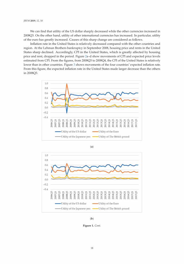
3.3. Movements of Utility of International Currencies
We use Equation (1) to calculate utility of international currency in each period. Figure 1a–d showtime series of utility of four international currencies. Throughout a whole period, changes in utility ofthe US dollar, the euro, the Japanese yen and the British pound are fluctuating around 0.5, 0.35, 0.03and 0.08, respectively.
2 An arithmetic average of real economic growth rates compared to the same quarter of previous year among the threecountries and the region (the United States, the euro zone, Japan, and the United Kingdom) was about 1.1% from 2006Q3 to2017Q4. However, if we exclude a period of 2008Q2 to 2010Q1 where the growth rate has greatly declined due to the globalfinancial crisis, it was about 1.8%. Given the real economic growth rates, our setting the values as a real interest rate seem tobe reasonable. The real economic growth rate data obtained from the OECD website.
3 We used a method of Fama and Gibbons (1984) to estimate expected inflation rates. However, a sample period is muchshorter than that by using the ARIMA model due to data constraints if we use the method. In addition, we could not use itbecause expected inflation rate of TIPS and survey data was only long-term expectation data, and Japan’s TIPS data was asmall sample. For those reasons, we choose to use the ARIMA model using CPI.
17
JRFM 2019, 12, 10
We can find that utility of the US dollar sharply decreased while the other currencies increased in2008Q3. On the other hand, utility of other international currencies has increased. In particular, utilityof the euro has greatly increased. Causes of this sharp change are considered as follows.
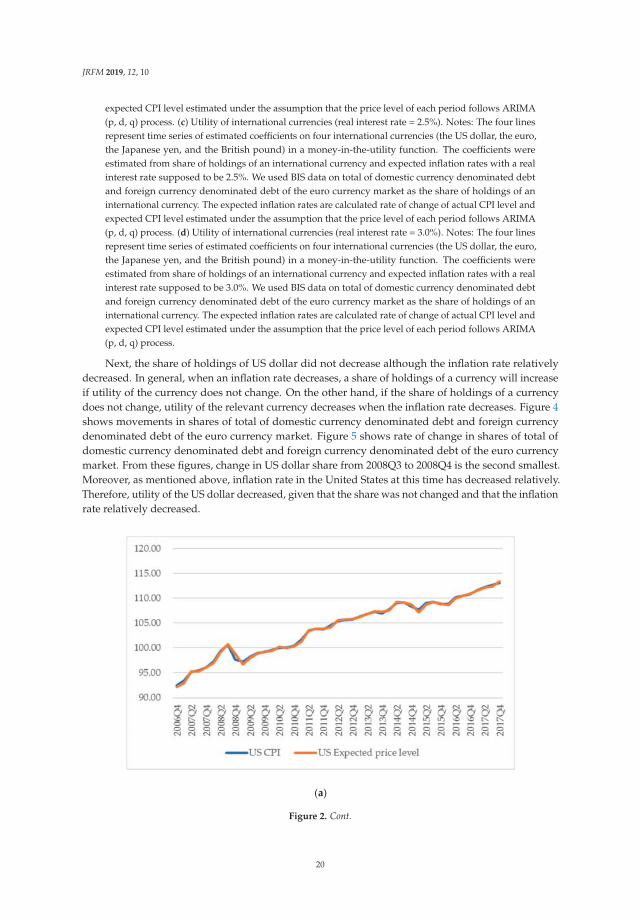
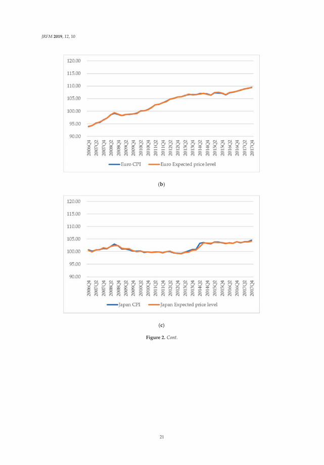
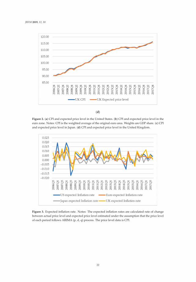
Inflation rate in the United States is relatively decreased compared with the other countries andregion. At the Lehman Brothers bankruptcy in September 2008, housing price and rents in the UnitedStates sharp declined. Accordingly, CPI in the United States, which is greatly affected by housingprice and rent, dropped in the period. Figure 2a–d show movements of CPI and expected price levelsestimated from CPI. From the figures, from 2008Q3 to 2008Q4, the CPI of the United States is relativelylower than in other countries. Figure 3 shows movements of the four countries’ expected inflation rate.From this figure, the expected inflation rate in the United States made larger decrease than the othersin 2008Q3.
(a)
(b)
Figure 1. Cont.
18
JRFM 2019, 12, 10
(c)
(d)
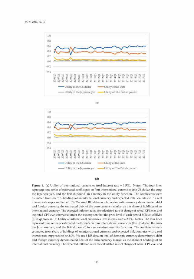
Figure 1. (a) Utility of international currencies (real interest rate = 1.5%). Notes: The four linesrepresent time series of estimated coefficients on four international currencies (the US dollar, the euro,the Japanese yen, and the British pound) in a money-in-the-utility function. The coefficients wereestimated from share of holdings of an international currency and expected inflation rates with a realinterest rate supposed to be 1.5%. We used BIS data on total of domestic currency denominated debtand foreign currency denominated debt of the euro currency market as the share of holdings of aninternational currency. The expected inflation rates are calculated rate of change of actual CPI level andexpected CPI level estimated under the assumption that the price level of each period follows ARIMA(p, d, q) process. (b) Utility of international currencies (real interest rate = 2.0%). Notes: The four linesrepresent time series of estimated coefficients on four international currencies (the US dollar, the euro,the Japanese yen, and the British pound) in a money-in-the-utility function. The coefficients wereestimated from share of holdings of an international currency and expected inflation rates with a realinterest rate supposed to be 2.0%. We used BIS data on total of domestic currency denominated debtand foreign currency denominated debt of the euro currency market as the share of holdings of aninternational currency. The expected inflation rates are calculated rate of change of actual CPI level and
19
JRFM 2019, 12, 10
expected CPI level estimated under the assumption that the price level of each period follows ARIMA(p, d, q) process. (c) Utility of international currencies (real interest rate = 2.5%). Notes: The four linesrepresent time series of estimated coefficients on four international currencies (the US dollar, the euro,the Japanese yen, and the British pound) in a money-in-the-utility function. The coefficients wereestimated from share of holdings of an international currency and expected inflation rates with a realinterest rate supposed to be 2.5%. We used BIS data on total of domestic currency denominated debtand foreign currency denominated debt of the euro currency market as the share of holdings of aninternational currency. The expected inflation rates are calculated rate of change of actual CPI level andexpected CPI level estimated under the assumption that the price level of each period follows ARIMA(p, d, q) process. (d) Utility of international currencies (real interest rate = 3.0%). Notes: The four linesrepresent time series of estimated coefficients on four international currencies (the US dollar, the euro,the Japanese yen, and the British pound) in a money-in-the-utility function. The coefficients wereestimated from share of holdings of an international currency and expected inflation rates with a realinterest rate supposed to be 3.0%. We used BIS data on total of domestic currency denominated debtand foreign currency denominated debt of the euro currency market as the share of holdings of aninternational currency. The expected inflation rates are calculated rate of change of actual CPI level andexpected CPI level estimated under the assumption that the price level of each period follows ARIMA(p, d, q) process.
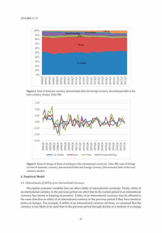
Next, the share of holdings of US dollar did not decrease although the inflation rate relativelydecreased. In general, when an inflation rate decreases, a share of holdings of a currency will increaseif utility of the currency does not change. On the other hand, if the share of holdings of a currencydoes not change, utility of the relevant currency decreases when the inflation rate decreases. Figure 4shows movements in shares of total of domestic currency denominated debt and foreign currencydenominated debt of the euro currency market. Figure 5 shows rate of change in shares of total ofdomestic currency denominated debt and foreign currency denominated debt of the euro currencymarket. From these figures, change in US dollar share from 2008Q3 to 2008Q4 is the second smallest.Moreover, as mentioned above, inflation rate in the United States at this time has decreased relatively.Therefore, utility of the US dollar decreased, given that the share was not changed and that the inflationrate relatively decreased.
(a)
Figure 2. Cont.
20
JRFM 2019, 12, 10
(b)
(c)
Figure 2. Cont.
21
JRFM 2019, 12, 10
(d)
Figure 2. (a) CPI and expected price level in the United States. (b) CPI and expected price level in theeuro zone. Notes: CPI is the weighted average of the original euro area. Weights are GDP share. (c) CPIand expected price level in Japan. (d) CPI and expected price level in the United Kingdom.
Figure 3. Expected inflation rate. Notes: The expected inflation rates are calculated rate of changebetween actual price level and expected price level estimated under the assumption that the price levelof each period follows ARIMA (p, d, q) process. The price level data is CPI.
22
JRFM 2019, 12, 10
Figure 4. Total of domestic currency denominated debt and foreign currency denominated debt of theeuro currency market. Data: BIS.
Figure 5. Rates of change of share of holdings of the international currencies. Data: BIS, rates of changeof total of domestic currency denominated debt and foreign currency denominated debt of the eurocurrency market.
4. Empirical Model
4.1. Determinants of Utility of an International Currency
We explain economic variables that can affect utility of international currencies. Firstly, utility ofan international currency in the previous period can affect that in the current period if an internationalcurrency has inertia in keeping its position. Utility of an international currency may be affected inthe same direction as utility of an international currency in the previous period if they have inertia interms of changes. For example, if utility of an international currency declines, we assumed that thecurrency is less likely to be used than in the previous period through decline of a medium of exchange
23

JRFM 2019, 12, 10
function and economies of scale. In other words, utility of an international currency has inertia interms of keeping changes in the same direction.
Secondly, supply of liquidity in terms of an international currency can affect its utility. A liquidityrisk premium in terms of an international currency is an indicator of a liquidity condition in terms ofthe relevant international currency or its liquidity shortage. A liquidity shortage reduces utility of aninternational currency through deteriorating its function as a medium of exchange.
Thirdly, an international currency is more likely to be used in proportion to economic activityin the relevant country. A larger volume of international economic transactions with the relevantcountry make the international currency more useful in terms of its function as a medium of exchangebecause of its network externalities. The economic activity in the relevant country and the volume ofinternational economic transactions with the relevant country can be represented by GDP, nominaleconomic growth rate, real economic growth rate, capitalization, total international trade, total exports,international capital flows, and money stock.
Fourthly, economic agents are likely to prefer a more stable value of currency in holding it asan international currency. Since standard deviation of nominal effective exchange rate is regardedas an indicator of the stability of relevant international currency, it can be a determinant of utility ofthe relevant international currency. In addition, economic agents are likely to prefer a higher valueof currency in holding it as an international currency. An effective exchange rate of an internationalcurrency, that is an indicator of a currency value against the other currencies, could be a determinantof utility of the relevant international currency.
4.2. A Dynamic Panel Model
We analyze determinants of utility of international currencies by using panel data. In addition,the explanatory variables include a lag term of utility of an international currency as we explainedabove. For the reasons, we use a dynamic panel data model to analyze determinants of utility ofinternational currencies. Given the above candidates for determinants of an international currency,a dynamic panel model is shown as follows:
Utility o f international currencyit= b1Utility o f international currencyit−1 + b2Liquidity risk premiumit+b3Money stock shareit + b4Relative nominal economic growthit+b5Relative real economic growthit + b6GDP shareit+b7Capitalization shareit + b8Total trade shareit + b9Total export shareit+b10Capital f low shareit + b11SD o f Nominal e f f ective exchange rateit+b12LN nominal e f f ective exchange rateit+b13LN real e f f ective exchange rateit + υi + εit
(2)
where υi: fixed effects, εit: disturbance term. We take a first difference of the above model (Equation (2))and remove fixed effects. Thus, its first difference model is rewritten as follows:
ΔUtility o f international currencyit= b1ΔUtility o f international currencyit−1 + b2ΔLiquidity risk premiumit+b3ΔMoney stock shareit + b4ΔRelative nominal economic growthit+b5ΔRelative real economic growthit + b6ΔGDP shareit+b7ΔCapitalization shareit + b8ΔTotal trade shareit + b9ΔTotal export shareit+b10ΔCapital f low shareit + b11ΔSD o f Nominal e f f ective exchange rateit+b12ΔLN nominal e f f ective exchange rateit+b13ΔLN real e f f ective exchange rateit + Δεit
(3)
where Δ: difference operator.
24
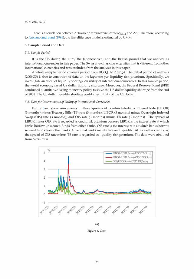
JRFM 2019, 12, 10
There is a correlation between ΔUtility o f international currencyit−1 and Δεit. Therefore, accordingto Arellano and Bond (1991), the first difference model is estimated by GMM.
5. Sample Period and Data
5.1. Sample Period
It is the US dollar, the euro, the Japanese yen, and the British pound that we analyze asinternational currencies in this paper. The Swiss franc has characteristics that is different from otherinternational currencies and was excluded from the analysis in this paper.
A whole sample period covers a period from 2006Q3 to 2017Q4. The initial period of analysis(2006Q3) is due to constraint of data on the Japanese yen liquidity risk premium. Specifically, weinvestigate an effect of liquidity shortage on utility of international currencies. In this sample period,the world economy faced US dollar liquidity shortage. Moreover, the Federal Reserve Board (FRB)conducted quantitative easing monetary policy to solve the US dollar liquidity shortage from the endof 2008. The US dollar liquidity shortage could affect utility of the US dollar.
5.2. Data for Determinants of Utility of International Currencies
Figure 6a–d show movements in three spreads of London Interbank Offered Rate (LIBOR)(3 months) minus Treasury Bills (TB) rate (3 months), LIBOR (3 months) minus Overnight IndexedSwap (OIS) rate (3 months), and OIS rate (3 months) minus TB rate (3 months). The spread ofLIBOR minus OIS rate is regarded as credit risk premium because LIBOR is the interest rate at whichbanks borrow unsecured funds from other banks. OIS rate is the interest rate at which banks borrowsecured funds from other banks. Given that banks mainly face and liquidity risk as well as credit risk,the spread of OIS rate minus TB rate is regarded as liquidity risk premium. The data were obtainedfrom Datastream.
−Δ Δ
(a)
Figure 6. Cont.
25

JRFM 2019, 12, 10
(b)
(c)
Figure 6. Cont.
26
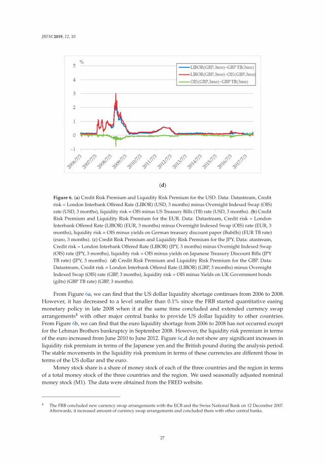
JRFM 2019, 12, 10
(d)
Figure 6. (a) Credit Risk Premium and Liquidity Risk Premium for the USD. Data: Datastream, Creditrisk = London Interbank Offered Rate (LIBOR) (USD, 3 months) minus Overnight Indexed Swap (OIS)rate (USD, 3 months), liquidity risk = OIS minus US Treasury Bills (TB) rate (USD, 3 months). (b) CreditRisk Premium and Liquidity Risk Premium for the EUR. Data: Datastream, Credit risk = LondonInterbank Offered Rate (LIBOR) (EUR, 3 months) minus Overnight Indexed Swap (OIS) rate (EUR, 3months), liquidity risk = OIS minus yields on German treasury discount paper (Bubills) (EUR TB rate)(euro, 3 months). (c) Credit Risk Premium and Liquidity Risk Premium for the JPY. Data: atastream,Credit risk = London Interbank Offered Rate (LIBOR) (JPY, 3 months) minus Overnight Indexed Swap(OIS) rate (JPY, 3 months), liquidity risk = OIS minus yields on Japanese Treasury Discount Bills (JPYTB rate) (JPY, 3 months). (d) Credit Risk Premium and Liquidity Risk Premium for the GBP. Data:Datastream, Credit risk = London Interbank Offered Rate (LIBOR) (GBP, 3 months) minus OvernightIndexed Swap (OIS) rate (GBP, 3 months), liquidity risk = OIS minus Yields on UK Government bonds(gilts) (GBP TB rate) (GBP, 3 months).
From Figure 6a, we can find that the US dollar liquidity shortage continues from 2006 to 2008.However, it has decreased to a level smaller than 0.1% since the FRB started quantitative easingmonetary policy in late 2008 when it at the same time concluded and extended currency swaparrangements4 with other major central banks to provide US dollar liquidity to other countries.From Figure 6b, we can find that the euro liquidity shortage from 2006 to 2008 has not occurred exceptfor the Lehman Brothers bankruptcy in September 2008. However, the liquidity risk premium in termsof the euro increased from June 2010 to June 2012. Figure 6c,d do not show any significant increases inliquidity risk premium in terms of the Japanese yen and the British pound during the analysis period.The stable movements in the liquidity risk premium in terms of these currencies are different those interms of the US dollar and the euro.
Money stock share is a share of money stock of each of the three countries and the region in termsof a total money stock of the three countries and the region. We used seasonally adjusted nominalmoney stock (M1). The data were obtained from the FRED website.
4 The FRB concluded new currency swap arrangements with the ECB and the Swiss National Bank on 12 December 2007.Afterwards, it increased amount of currency swap arrangements and concluded them with other central banks.
27

JRFM 2019, 12, 10
GDP share is a share of GDP of each of the three countries and the region in terms of a total GDPof the three countries and the region (the United State, the euro Area, Japan, the United Kingdom). Weused seasonally adjusted nominal GDP for the calculation. The data were obtained from the IFS ofIMF website.
Relative nominal economic growth rate and relative real economic growth rate are ratio of GDPgrowth rate of each of the three countries and the region in terms of an arithmetic average of GDPgrowth rate of the three countries and the region. Nominal economic growth rate compared to previousquarter was calculated from seasonally adjusted nominal GDP. In addition, we used seasonally adjustedreal economic growth rate compared to previous quarter to calculate a relative real economic growthrate. The data were obtained from the Organization for Economic Co-operation and Development(OECD) website.
Capitalization share is a share of capitalization of each of the three countries and the region interms of a total capitalization of the three countries and the region. We could not obtain the data ofUnited Kingdom in 2010 and quarterly data of the three countries and the region. For the reason,we estimated quarterly data using linear interpolation from annual data. We used data on marketcapitalization of listed domestic companies for the calculation. The data were obtained from websiteof the World Bank and the ECB.
Total trade share is a share of trade amount of each of the three countries and the region in termsof a total trade amount of the three countries and the region with the rest of the world. When wesum up the total trade amount for the three countries and the region, we exclude exports and importsamong them. Also, total export share is a share of export value of each of the three countries and theregion in terms of a total export value of the three countries and the region with the rest of the world.The data were obtained from the Direction of Trade Statistics of IMF website.
Capital flow share is a share of international capital flows of each of the three countries and theregion in terms of a total international capital flows of the three countries and the region. We couldnot obtain quarterly data of Japan for 2006Q3 to 2010Q1. For the reason, we estimated quarterly datausing linear interpolation from annual data. In this paper, the international capital flows are defined assum of values of direct investments, portfolio investments, and other investments of net acquisition offinancial assets and direct investments, portfolio investments, and other investments of net incurrenceof liabilities. The data were obtained from the Balance of Payments and International Investment Positionof IMF website.
Data on both nominal and real effective exchange rates of each of the currencies are takenlogarithms. The data were obtained from BIS website and the IFS of IMF website. Table 1 shows meanand standard deviation of difference of each variable.
28
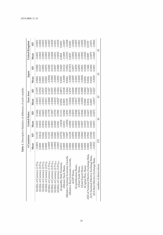
JRFM 2019, 12, 10
Ta
ble
1.
Des
crip
tive
Stat
isti
csof
diff
eren
ceof
each
vari
able
.
4C
ou
ntr
ies
Un
ite
dS
tate
sE
uro
Are
aJa
pa
nU
nit
ed
Kin
gd
om
Me
an
SD
Me
an
SD
Me
an
SD
Me
an
SD
Me
an
SD
ΔU
tilit
yof
Cur
renc
y(1
.5%
) t−0
.000
10.
1153
0.00
100.
1666
−0.0
015
0.13
750.
0004
0.02
80−0
.000
1−0
.000
1Δ
Uti
lity
ofC
urre
ncy
(2.0
%) t
0.00
000.
0614
0.00
100.
0921
−0.0
013
0.07
430.
0003
0.01
27−0
.000
2−0
.000
2Δ
Uti
lity
ofC
urre
ncy
(2.5
%) t
0.00
000.
0441
0.00
100.
0665
−0.0
012
0.05
370.
0003
0.00
92−0
.000
3−0
.000
3Δ
Uti
lity
ofC
urre
ncy
(3.0
%) t
0.00
000.
0352
0.00
100.
0530
−0.0
011
0.04
300.
0002
0.00
76−0
.000
3−0
.000
3Δ
Uti
lity
ofC
urre
ncy
(1.5
%) t-
1−0
.000
50.
1221
0.00
930.
1778
−0.0
068
0.14
37−0
.000
40.
0285
−0.0
043
−0.0
043
ΔU
tilit
yof
Cur
renc
y(2
.0%
) t-1
−0.0
003
0.06
660.
0063
0.10
07−0
.004
40.
0787
−0.0
002
0.01
32−0
.002
8−0
.002
8Δ
Uti
lity
ofC
urre
ncy
(2.5
%) t-
1−0
.000
20.
0481
0.00
490.
0730
−0.0
033
0.05
69−0
.000
20.
0097
−0.0
021
−0.0
021
ΔU
tilit
yof
Cur
renc
y(3
.0%
) t-1
−0.0
001
0.03
830.
0041
0.05
82−0
.002
70.
0454
−0.0
001
0.00
80−0
.001
8−0
.001
8Δ
Liqu
idit
yR
isk
Prem
ium
t0.
0012
0.07
54−0
.003
60.
1111
0.00
540.
0873
0.00
280.
0429
0.00
040.
0003
ΔM
oney
Stoc
kSh
are t
0.00
000.
0087
0.00
120.
0040
0.00
030.
0108
−0.0
009
0.01
22−0
.000
9−0
.000
7Δ
Rel
ativ
eN
omin
alEc
onom
icG
row
tht
0.00
003.
9457
−0.0
054
1.47
810.
0199
3.42
640.
0064
5.05
24−0
.037
0−0
.020
8Δ
Rel
ativ
eR
ealE
cono
mic
Gro
wth
t0.
0000
6.61
280.
0058
3.22
96−0
.002
45.
4797
−0.0
083
10.7
073
0.00
550.
0049
ΔG
DP
Shar
e t0.
0000
0.00
590.
0012
0.00
74−0
.000
40.
0049
−0.0
007
0.00
77−0
.000
2−0
.000
2Δ
Cap
ital
izat
ion
Shar
e t0.
0000
0.00
420.
0025
0.00
44−0
.001
70.
0046
−0.0
001
0.00
39−0
.000
7−0
.000
7Δ
Tota
lTra
deSh
are t
0.00
000.
0068
0.00
050.
0072
−0.0
002
0.01
02−0
.000
20.
0050
−0.0
001
−0.0
001
ΔTo
talE
xpor
tSha
ret
0.00
000.
0060
0.00
070.
0044
−0.0
002
0.00
88−0
.000
40.
0061
−0.0
002
−0.0
002
ΔC
apit
alFl
owSh
are t
0.00
000.
0049
0.00
100.
0060
0.00
060.
0060
0.00
040.
0028
−0.0
020
−0.0
020
ΔSD
ofN
omin
alEf
fect
ive
Exch
ange
Rat
e t0.
0082
0.99
410.
0107
0.64
150.
0016
0.66
470.
0046
1.34
460.
0089
0.01
59Δ
LNN
omin
alEf
fect
ive
Exch
ange
Rat
e t−0
.000
50.
0340
0.00
230.
0281
0.00
070.
0227
0.00
200.
0494
−0.0
075
−0.0
071
ΔLN
Rea
lEff
ecti
veEx
chan
geR
ate t
−0.0
023
0.03
390.
0015
0.02
72−0
.001
70.
0227
−0.0
029
0.04
91−0
.006
5−0
.006
0
num
ber
ofob
serv
atio
ns17
243
4343
43
29
JRFM 2019, 12, 10
6. Empirical Analysis on Determinants of Utility of International Currencies
6.1. Expected Effect of Determinant on Utility of International Currencies
We expect that each of determinants affects utility of international currencies in as a directionas follows.
If there is inertia of an international currency in terms of changes in utility, a change in utilityof an international currency in the previous period has a positive effect on a change in utility ofthe international currency in the current period. For example, if utility of an international currencydeclines, demand for the relevant international currency as one with a function as medium of exchangeshould decrease. The decrease in the demand for the international currency, in turn, makes utilityof an international currency decline further. We investigate a hypothesis that a change in utilityof an international currency in the previous period has a positive effect on change in utility of theinternational currency in the current period.
An increase in the liquidity risk premium in terms of an international currency means liquidityshortage in terms of the relevant international currency. The liquidity shortage reduces convenience ofthe international currency for economic agents to use for medium of exchange. Thus, an occurrenceof liquidity shortage decreases utility of the international currency. The liquidity risk premium, thatis indicated by OIS rate minus TB rate, increases when the liquidity shortage worsens. Therefore, anincrease in the liquidity risk premium reduces utility of the international currency. We investigate ahypothesis that liquidity risk premium has a negative effect on utility of the international currency.Figures 1a–d and 2a show that both we had both the increase in the US dollar liquidity risk premiumin 2008 and the decrease in utility of the US dollar in 2008Q3 simultaneously.
Money stock share, relative nominal economic growth rate, relative real economic growth rate,GDP share, capitalization share, total trade share, total export share, and capital flow share areeconomic variables that represent relative economic size of the relevant country. Network externalitiesworks in selecting an international currency as medium of exchange. For the reason, a change inan economic size of the relevant country has a positive effect on utility of the international currency.We investigate a hypothesis that coefficients of explanatory variables that represent relative economicsize are positive.
As we have already explained, economic agents are likely to prefer a stabler and higher valueof currency in holding it as an international currency. The standard deviation and value of effectiveexchange rate of an international currency, that is an indicator of a currency stable and value against theother currencies, could be a determinant of utility of the relevant international currency. We investigatea hypothesis that a stabler and higher value of an international currency increase. We analyze whetheran increase in an effective exchange rate increases utility of the relevant international currency.
6.2. Empirical Results
Tables 2–5 show results of the dynamic panel analysis. A head line in Tables represents empiricalanalysis number. Table 2 shows determinants of utility of international currency supposing that areal interest rate is 1.5%. Coefficients on change in utility of international currencies in the previousperiod are significantly positive in 26 cases of total 36 cases. The coefficients are estimated from 0.15to 0.26. Coefficients on change in liquidity risk premium are significantly negative in all of the casesat 1% of significance level. The coefficients are estimated from −0.25 to −0.20. In the analyses 1 to4 and 12, the coefficients on change in money stock share are positive at 10% of significance level.The coefficients are estimated from 3.50 to 3.72. In the analyses 1 to 12 and 36, the coefficients onchange in capital flow share are significantly positive. The coefficients are estimated from 1.21 to 2.93.However, economic scale variables excluding money stock share and capital flow share and effectiveexchange rate related variables do not satisfy a sign condition or significance levels.
Table 3 shows determinants of utility of international currency supposing that a real interestrate is 2.0%. Coefficients on change in utility of international currencies in the previous period are
30

JRFM 2019, 12, 10
significantly positive in 20 cases of total 36 cases. The coefficients are estimated from 0.22 to 0.40.Coefficients on change in liquidity risk premium are significantly negative in all of the cases at 1% ofsignificance level. The coefficients are estimated from −0.11 to −0.08. In the analysis 49, the coefficientson change in money stock share are positive at 5% of significance level. The coefficient is estimated0.58. Coefficients on change in capital flow share are significantly positive in all of the cases at thesignificance level 1%. The coefficients are estimated from 0.86 to 1.71. In the analysis 62, Coefficientson change in nominal effective exchange rate are significantly positive at the significance level 10%.The coefficients are estimated 0.30. However, most of the coefficients on change in economic variablesassociated with relative economic scale excluding capital flow share and effective exchange rate do notsatisfy a sign condition or significance levels.
Table 4 shows determinants of utility of international currency supposing that a real interest rate is2.5%. Coefficients on change in utility of international currencies in the previous period are significantlypositive in 22 cases of total 36 cases. The coefficients are estimated from 0.16 to 0.45. Coefficients onchange in liquidity risk premium are significantly negative in all of the cases. The coefficients areestimated from −0.07 to −0.04. In the analysis 85, the coefficients on change in money stock share arepositive at 5% of significance level. The coefficient is estimated 0.42. Coefficients on change in capitalflow share are significantly positive in all of the cases except analysis 84. The coefficients are estimatedfrom 0.65 to 1.07. In the analysis 98, the coefficients on change in nominal effective exchange rate arepositive at 10% of significance level. The coefficient is estimated 0.24. However, most of the coefficientson change in economic variables associated with relative economic scale excluding capital flow shareand effective exchange rate do not satisfy a sign condition or significance levels.
Table 5 shows determinants of utility of international currency supposing that a real interest rate is3.0%. Coefficients on change in utility of international currencies in the previous period are significantlypositive in 23 cases of total 36 cases. The coefficients are estimated to be from 0.06 to 0.43. Coefficientson change in utility of international currencies in the previous period are significantly negative in14 cases out of 36 cases. The coefficients are estimated to be −0.04 and −0.03. In the analyses 136and 144, coefficients on change in capital flow share are significantly positive. The coefficients areestimated to be 0.45 and 0.51. However, most of the coefficients on change in economic variablesassociated with relative economic scale and effective exchange rate do not satisfy the sign condition orthe significance level.
We summarize the above empirical results. Firstly, the coefficients on utility of internationalcurrency in the previous period are significantly positive in the many cases. These results suggest thatchange in utility of an international currency in the previous period in the same direction has effect onchange in utility of the international currency in the current period. There is inertia in terms of changein the international monetary system.
Secondly, the coefficients on liquidity risk premium are significantly negative in all of the casesexcept the real interest rate 3.0%. Even if the real interest rate is 3.0%, liquidity risk premium issignificantly negative in about half of cases. The empirical result is consistent with the hypothesisthat liquidity risk premium has a negative effect on utility of the international currency. We find thatutility of an international currency is affected by liquidity condition or liquidity shortage. Specifically,the liquidity shortage reduces utility of the international currency through a reduction in conveniencefor economic agents to use the relevant international currency as a medium of exchange.
Thirdly, the coefficients on capital flow share are significant in many cases except in cases ofreal interest rate 3.0%. Capital flow share represent relative economic scale of the relevant country.Therefore, the above results suggest that utility of the international currency might be affected bychanges in economic scale. However, since other economic scale variables did not become significant,the relative change in capital flows may be affecting utility of the international currency.
31

JRFM 2019, 12, 10
Ta
ble
2.
Det
erm
inan
tsut
ility
ofin
tern
atio
nalc
urre
ncy
(rea
lint
eres
trat
e1.
5%).
12
34
56
78
910
11
12
13
14
15
16
17
18
ΔU
tilit
yof
inte
rnat
iona
lcu
rren
cyit
-1
0.14
0.23
0.13
0.23
*0.
160.
26*
0.16
0.26
*0.
150.
24*
0.14
0.24
*0.
21**
0.20
**0.
20**
0.21
**0.
21**
0.06
(0.3
0)(0
.10)
(0.2
8)(0
.09)
(0.2
5)(0
.07)
(0.2
2)(0
.05)
(0.2
8)(0
.08)
(0.2
7)(0
.07)
(0.0
1)(0
.05)
(0.0
4)(0
.02)
(0.0
2)(0
.43)
ΔLi
quid
ity
risk
prem
ium
it−0
.21
***
−0.2
4**
*−0
.21
***
−0.2
3**
*−0
.22
***
−0.2
5**
*−0
.22
***
−0.2
4**
*−0
.22
***
−0.2
5**
*−0
.22
***
−0.2
4**
*−0
.19
***
−0.2
1**
*−0
.21
***
−0.2
2**
*−0
.21
***
−0.2
3**
*(0
.00)
(0.0
0)(0
.00)
(0.0
0)(0
.00)
(0.0
0)(0
.00)
(0.0
0)(0
.00)
(0.0
0)(0
.00)
(0.0
0)(0
.00)
(0.0
0)(0
.00)
(0.0
0)(0
.00)
(0.0
0)
ΔM
oney
stoc
ksh
are i
t3.
50*
3.55
*3.
57*
3.64
*3.
363.
493.
443.
583.
503.
623.
603.
72*
0.85
(0.0
7)(0
.06)
(0.0
7)(0
.06)
(0.1
5)(0
.13)
(0.1
4)(0
.12)
(0.1
1)(0
.10)
(0.1
0)(0
.09)
(0.1
9)
ΔR
elat
ive
nom
inal
econ
omic
grow
thit
−0.0
007
−0.0
015
−0.0
008
−0.0
017
−0.0
009
−0.0
017
−0.0
020
(0.6
3)(0
.35)
(0.5
9)(0
.33)
(0.5
8)(0
.33)
(0.3
2)
ΔR
elat
ive
real
econ
omic
grow
thit
−0.0
005
−0.0
006
−0.0
005
−0.0
006
−0.0
006
−0.0
006
−0.0
003
(0.4
6)(0
.30)
(0.4
4)(0
.25)
(0.4
1)(0
.23)
(0.5
7)
ΔG
DP
shar
e it
−2.9
7−3
.71
−2.9
7−3
.66
−3.6
9−4
.47
−3.6
2−4
.38
*−3
.46
−4.2
3−3
.39
−4.1
4−0
.31
(0.3
2)(0
.17)
(0.3
1)(0
.15)
(0.2
4)(0
.11)
(0.2
3)(0
.10)
(0.2
6)(0
.12)
(0.2
6)(0
.11)
(0.6
7)
ΔC
apit
aliz
atio
nsh
are i
t−0
.02
−0.2
9−0
.04
−0.2
80.
13−0
.15
0.07
−0.1
8−0
.03
−0.3
0−0
.10
−0.3
5−0
.03
(0.9
8)(0
.84)
(0.9
6)(0
.84)
(0.9
0)(0
.93)
(0.9
4)(0
.91)
(0.9
8)(0
.85)
(0.9
0)(0
.82)
(0.8
8)
ΔTo
talt
rade
shar
e it
−5.7
8**
*−5
.83
***
−5.7
1**
*−5
.74
***
−5.7
2**
*−5
.75
***
−4.6
7**
*(0
.00)
(0.0
0)(0
.00)
(0.0
0)(0
.00)
(0.0
0)(0
.00)
ΔTo
tale
xpor
tsha
reit
−3.4
5*
−3.5
6*
−3.4
1*
−3.5
0*
−3.4
8*
−3.5
6*
(0.0
7)(0
.08)
(0.0
8)(0
.08)
(0.0
8)(0
.08)
ΔC
apit
alflo
wsh
are i
t2.
36**
*2.
36**
2.34
***
2.30
**2.
85**
*2.
93**
*2.
78**
*2.
83**
2.83
***
2.91
**2.
76**
*2.
81**
(0.0
0)(0
.02)
(0.0
0)(0
.03)
(0.0
0)(0
.01)
(0.0
0)(0
.02)
(0.0
0)(0
.02)
(0.0
0)(0
.04)
ΔSD
ofN
omin
alef
fect
ive
exch
ange
rate
it
−0.0
1−0
.01
**−0
.01
−0.0
1**
−0.0
2−0
.02
−0.0
2−0
.02
−0.0
2−0
.01
(0.1
6)(0
.04)
(0.1
6)(0
.04)
(0.2
5)(0
.24)
(0.2
5)(0
.26)
(0.2
3)(0
.36)
ΔLN
Nom
inal
effe
ctiv
eex
chan
gera
teit
0.15
0.13
0.14
0.13
(0.6
5)(0
.72)
(0.6
5)(0
.71)
ΔLN
Rea
leff
ecti
veex
chan
gera
teit
0.05
0.04
0.05
0.04
(0.8
7)(0
.92)
(0.8
9)(0
.91)
Sarg
ante
st0.
950.
970.
950.
970.
990.
990.
990.
990.
980.
990.
980.
990.
970.
980.
980.
970.
980.
87
AR
(1)s
eria
lco
rrel
atio
nte
st0.
08*
0.10
*0.
08*
0.10
*0.
08*
0.10
0.08
*0.
100.
08*
0.10
*0.
08*
0.10
*0.
09*
0.10
*0.
10*
0.10
*0.
100.
08*
AR
(2)s
eria
lco
rrel
atio
nte
st0.
470.
200.
580.
220.
970.
230.
880.
270.
860.
230.
950.
260.
180.
190.
190.
180.
180.
13
32

JRFM 2019, 12, 10
Ta
ble
2.
Con
t.
19
20
21
22
23
24
25
26
27
28
29
30
31
32
33
34
35
36
ΔU
tilit
yof
inte
rnat
iona
lcu
rren
cyit
-1
0.15
**0.
22**
0.21
**0.
23**
0.23
**0.
23**
0.23
**0.
070.
16*
0.25
***
0.20
**0.
22**
0.22
**0.
23**
0.23
**0.
070.
16*
0.25
**(0
.05)
(0.0
1)(0
.04)
(0.0
2)(0
.02)
(0.0
2)(0
.04)
(0.5
0)(0
.09)
(0.0
1)(0
.04)
(0.0
3)(0
.03)
(0.0
2)(0
.04)
(0.5
1)(0
.10)
(0.0
1)
ΔLi
quid
ity
risk
prem
ium
it−0
.25
***
−0.2
1**
*−0
.20
***
−0.2
1**
*−0
.20
***
−0.2
1**
*−0
.20
***
−0.2
2**
*−0
.24
***
−0.2
1**
*−0
.20
***
−0.2
1**
*−0
.21
***
−0.2
1**
*−0
.20
***
−0.2
2**
*−0
.24
***
−0.2
2**
*(0
.00)
(0.0
0)(0
.00)
(0.0
0)(0
.00)
(0.0
0)(0
.00)
(0.0
0)(0
.00)
(0.0
0)(0
.00)
(0.0
0)(0
.00)
(0.0
0)(0
.00)
(0.0
0)(0
.00)
(0.0
0)
ΔM
oney
stoc
ksh
are i
t0.
610.
90(0
.47)
(0.2
3)
ΔR
elat
ive
nom
inal
econ
omic
grow
thit
−0.0
019
−0.0
020
(0.3
5)(0
.34)
ΔR
elat
ive
real
econ
omic
grow
thit
−0.0
002
−0.0
002
(0.5
6)(0
.55)
ΔG
DP
shar
e it
−1.8
3**
*−1
.68
**(0
.00)
(0.0
1)
ΔC
apit
aliz
atio
nsh
are i
t−0
.31
−0.2
3(0
.57)
(0.7
1)
ΔTo
talt
rade
shar
e it
−5.5
7**
*−5
.52
***
(0.0
0)(0
.00)
ΔTo
tale
xpor
tsha
reit
−2.7
0−3
.56
*−3
.55
*(0
.11)
(0.0
7)(0
.06)
ΔC
apit
alflo
wsh
are i
t1.
001.
051.
21*
(0.2
6)(0
.15)
(0.0
6)
ΔSD
ofN
omin
alef
fect
ive
exch
ange
rate
it
−0.0
1−0
.02
(0.2
6)(0
.16)
ΔLN
Nom
inal
effe
ctiv
eex
chan
gera
teit
0.01
0.14
0.17
0.45
0.17
0.43
0.33
0.11
(0.9
7)(0
.58)
(0.5
0)(0
.10)
(0.5
1)(0
.18)
(0.2
9)(0
.67)
ΔLN
Rea
leff
ecti
veex
chan
gera
teit
−0.0
90.
090.
120.
390.
120.
400.
300.
04(0
.78)
(0.7
2)(0
.62)
(0.1
5)(0
.64)
(0.1
9)(0
.32)
(0.8
6)
Sarg
ante
st0.
940.
980.
981.
001.
001.
001.
000.
980.
991.
000.
971.
001.
001.
001.
000.
980.
991.
00
AR
(1)s
eria
lco
rrel
atio
nte
st0.
09*
0.09
*0.
09*
0.10
*0.
10*
0.10
0.10
*0.
08*
0.09
*0.
09*
0.09
*0.
10*
0.10
*0.
100.
100.
08*
0.09
*0.
09*
AR
(2)s
eria
lco
rrel
atio
nte
st0.
160.
200.
210.
260.
250.
320.
240.
510.
160.
270.
210.
260.
250.
320.
240.
470.
160.
26
The
pare
nthe
ses
are
p-va
lue.
*,**
,***
are
sign
ifica
nce
leve
l10%
,5%
,1%
.Ins
trum
entv
aria
bles
for
peri
odta
reut
ility
ofth
ein
tern
atio
nalc
urre
ncy
ofpe
riod
st-
3.Th
enu
llhy
poth
esis
ofSa
rgan
test
isth
atov
er-i
dent
ifica
tion
isva
lid.T
henu
llhy
poth
esis
ofA
R(1
)and
AR
(2)s
eria
lcor
rela
tion
test
isth
atth
ere
isno
seri
alco
rrel
atio
n.
33
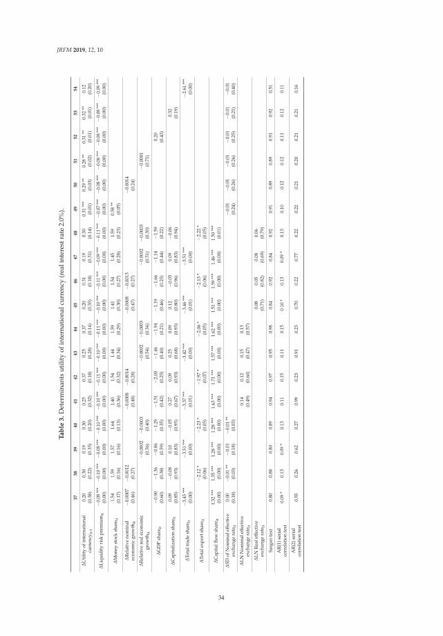
JRFM 2019, 12, 10
Ta
ble
3.
Det
erm
inan
tsut
ility
ofin
tern
atio
nalc
urre
ncy
(rea
lint
eres
trat
e2.
0%).
37
38
39
40
41
42
43
44
45
46
47
48
49
50
51
52
53
54
ΔU
tilit
yof
inte
rnat
iona
lcu
rren
cyit
-1
0.20
0.30
0.19
0.30
0.25
0.37
0.25
0.37
0.20
0.31
0.19
0.30
0.31
***
0.29
**0.
28**
0.31
**0.
32**
0.12
(0.3
8)(0
.22)
(0.3
5)(0
.20)
(0.3
2)(0
.18)
(0.2
8)(0
.14)
(0.3
5)(0
.18)
(0.3
1)(0
.14)
(0.0
1)(0
.03)
(0.0
2)(0
.01)
(0.0
1)(0
.20)
ΔLi
quid
ity
risk
prem
ium
it−0
.08
***
−0.1
0**
*−0
.08
***
−0.1
0**
*−0
.10
***
−0.1
1**
*−0
.10
***
−0.1
1**
*−0
.10
***
−0.1
1**
*−0
.09
***
−0.1
1**
*−0
.07
***
−0.0
8**
*−0
.08
***
−0.0
8**
*−0
.08
***
−0.0
9**
*(0
.00)
(0.0
0)(0
.00)
(0.0
0)(0
.00)
(0.0
0)(0
.00)
(0.0
0)(0
.00)
(0.0
0)(0
.00)
(0.0
0)(0
.00)
(0.0
0)(0
.00)
(0.0
0)(0
.00)
(0.0
0)
ΔM
oney
stoc
ksh
are i
t1.
541.
591.
571.
641.
401.
541.
441.
591.
411.
541.
451.
590.
58**
(0.1
7)(0
.16)
(0.1
6)(0
.13)
(0.3
6)(0
.32)
(0.3
4)(0
.29)
(0.3
0)(0
.27)
(0.2
8)(0
.23)
(0.0
5)
ΔR
elat
ive
nom
inal
econ
omic
grow
thit
−0.0
007
−0.0
012
−0.0
008
−0.0
014
−0.0
008
−0.0
013
−0.0
014
(0.4
6)(0
.27)
(0.4
8)(0
.28)
(0.4
7)(0
.27)
(0.2
4)
ΔR
elat
ive
real
econ
omic
grow
thit
−0.0
002
−0.0
003
−0.0
002
−0.0
003
−0.0
002
−0.0
003
−0.0
001
(0.5
6)(0
.40)
(0.5
4)(0
.34)
(0.5
1)(0
.30)
(0.7
1)
ΔG
DP
shar
e it
−0.9
0−1
.36
−0.8
6−1
.29
−1.5
1−2
.00
−1.4
6−1
.94
−1.1
9−1
.66
−1.1
4−1
.59
0.20
(0.6
0)(0
.38)
(0.5
9)(0
.35)
(0.4
2)(0
.25)
(0.4
0)(0
.21)
(0.4
6)(0
.25)
(0.4
4)(0
.22)
(0.4
3)
ΔC
apit
aliz
atio
nsh
are i
t0.
09−0
.08
0.10
−0.0
50.
270.
090.
250.
090.
12−0
.05
0.09
−0.0
60.
32(0
.85)
(0.9
3)(0
.83)
(0.9
5)(0
.67)
(0.9
3)(0
.68)
(0.9
3)(0
.80)
(0.9
6)(0
.83)
(0.9
4)(0
.19)
ΔTo
talt
rade
shar
e it
−3.4
5**
*−3
.51
***
−3.3
7**
*−3
.42
***
−3.4
6**
*−3
.51
***
−2.6
1**
*(0
.00)
(0.0
0)(0
.01)
(0.0
0)(0
.01)
(0.0
0)(0
.00)
ΔTo
tale
xpor
tsha
reit
−2.1
2*
−2.2
3*
−1.9
7*
−2.0
6*
−2.1
3*
−2.2
2*
(0.0
6)(0
.05)
(0.0
7)(0
.05)
(0.0
6)(0
.05)
ΔC
apit
alflo
wsh
are i
t1.
32**
*1.
35**
*1.
28**
*1.
28**
*1.
63**
*1.
71**
*1.
57**
*1.
62**
*1.
51**
*1.
59**
*1.
46**
*1.
50**
*(0
.00)
(0.0
0)(0
.00)
(0.0
0)(0
.00)
(0.0
0)(0
.00)
(0.0
0)(0
.00)
(0.0
0)(0
.00)
(0.0
1)
ΔSD
ofN
omin
alef
fect
ive
exch
ange
rate
it
0.00
−0.0
1**
−0.0
1−0
.01
**−0
.01
−0.0
1−0
.01
−0.0
1−0
.01
−0.0
1(0
.18)
(0.0
3)(0
.18)
(0.0
3)(0
.24)
(0.2
6)(0
.26)
(0.2
5)(0
.21)
(0.4
0)
ΔLN
Nom
inal
effe
ctiv
eex
chan
gera
teit
0.14
0.12
0.15
0.13
(0.4
9)(0
.60)
(0.4
7)(0
.57)
ΔLN
Rea
leff
ecti
veex
chan
gera
teit
0.08
0.05
0.08
0.06
(0.7
1)(0
.82)
(0.6
9)(0
.79)
Sarg
ante
st0.
800.
880.
800.
890.
940.
970.
950.
980.
840.
920.
840.
920.
910.
890.
890.
910.
920.
51
AR
(1)s
eria
lco
rrel
atio
nte
st0.
09*
0.13
0.09
*0.
130.
110.
150.
110.
150.
10*
0.13
0.09
*0.
130.
100.
120.
120.
110.
120.
11
AR
(2)s
eria
lco
rrel
atio
nte
st0.
550.
260.
620.
270.
990.
230.
910.
230.
700.
220.
770.
220.
220.
210.
200.
210.
210.
16
34

JRFM 2019, 12, 10
Ta
ble
3.
Con
t.
55
56
57
58
59
60
61
62
63
64
65
66
67
68
69
70
71
72
ΔU
tilit
yof
inte
rnat
iona
lcu
rren
cyit
-1
0.22
**0.
34**
0.31
**0.
36**
*0.
36**
*0.
37**
*0.
38**
0.16
0.27
*0.
40**
*0.
29**
0.35
***
0.35
***
0.36
***
0.37
**0.
160.
26*
0.40
**(0
.03)
(0.0
1)(0
.01)
(0.0
0)(0
.00)
(0.0
0)(0
.01)
(0.2
4)(0
.05)
(0.0
1)(0
.01)
(0.0
0)(0
.00)
(0.0
0)(0
.02)
(0.2
5)(0
.06)
(0.0
1)
ΔLi
quid
ity
risk
prem
ium
it−0
.09
***
−0.0
9**
*−0
.08
***
−0.0
9**
*−0
.09
***
−0.0
8**
*−0
.09
***
−0.0
9**
*−0
.10
***
−0.1
0**
*−0
.08
***
−0.0
9**
*−0
.09
***
−0.0
9**
*−0
.09
***
−0.0
9**
*−0
.10
***
−0.1
0**
*(0
.00)
(0.0
0)(0
.00)
(0.0
0)(0
.00)
(0.0
0)(0
.00)
(0.0
0)(0
.00)
(0.0
0)(0
.00)
(0.0
0)(0
.00)
(0.0
0)(0
.00)
(0.0
0)(0
.00)
(0.0
0)
ΔM
oney
stoc
ksh
are i
t0.
290.
44(0
.61)
(0.4
3)
ΔR
elat
ive
nom
inal
econ
omic
grow
thit
−0.0
014
−0.0
014
(0.2
8)(0
.27)
ΔR
elat
ive
real
econ
omic
grow
thit
−0.0
001
−0.0
001
(0.7
5)(0
.76)
ΔG
DP
shar
e it
−0.6
2**
*−0
.49
**(0
.00)
(0.0
2)
ΔC
apit
aliz
atio
nsh
are i
t0.
150.
21(0
.81)
(0.7
5)
ΔTo
talt
rade
shar
e it
−3.2
9**
*−3
.25
***
(0.0
0)(0
.00)
ΔTo
tale
xpor
tsha
reit
−1.4
5*
−2.0
1*
−2.0
2**
(0.0
7)(0
.05)
(0.0
5)
ΔC
apit
alflo
wsh
are i
t0.
89**
*0.
86**
*0.
97**
*(0
.00)
(0.0
0)(0
.00)
ΔSD
ofN
omin
alef
fect
ive
exch
ange
rate
it
−0.0
1−0
.01
*(0
.29)
(0.0
9)
ΔLN
Nom
inal
effe
ctiv
eex
chan
gera
teit
0.07
0.12
0.14
0.25
0.14
0.30
*0.
240.
09(0
.76)
(0.3
6)(0
.28)
(0.1
7)(0
.36)
(0.1
0)(0
.16)
(0.5
2)
ΔLN
Rea
leff
ecti
veex
chan
gera
teit
0.00
0.09
0.11
0.20
0.10
0.29
0.22
0.05
(0.9
9)(0
.47)
(0.3
6)(0
.25)
(0.4
8)(0
.11)
(0.1
7)(0
.72)
Sarg
ante
st0.
790.
940.
950.
990.
990.
990.
990.
930.
980.
990.
910.
980.
990.
990.
990.
920.
970.
99
AR
(1)s
eria
lco
rrel
atio
nte
st0.
120.
110.
110.
110.
110.
120.
110.
10*
0.11
0.10
0.11
0.11
0.12
0.12
0.12
0.10
0.12
0.11
AR
(2)s
eria
lco
rrel
atio
nte
st0.
180.
220.
210.
250.
240.
260.
240.
720.
170.
250.
210.
250.
230.
250.
240.
660.
170.
25
The
pare
nthe
ses
are
p-va
lue.
*,**
,***
are
sign
ifica
nce
leve
l10%
,5%
,1%
.Ins
trum
entv
aria
bles
for
peri
odta
reut
ility
ofth
ein
tern
atio
nalc
urre
ncy
ofpe
riod
st-
3.Th
enu
llhy
poth
esis
ofSa
rgan
test
isth
atov
er-i
dent
ifica
tion
isva
lid.T
henu
llhy
poth
esis
ofA
R(1
)and
AR
(2)s
eria
lcor
rela
tion
test
isth
atth
ere
isno
seri
alco
rrel
atio
n.
35

JRFM 2019, 12, 10
Ta
ble
4.
Det
erm
inan
tsut
ility
ofin
tern
atio
nalc
urre
ncy
(rea
lint
eres
trat
e2.
5%).
73
74
75
76
77
78
79
80
81
82
83
84
85
86
87
88
89
90
ΔU
tilit
yof
inte
rnat
iona
lcu
rren
cyit
-1
0.12
0.23
0.12
0.22
0.20
0.32
0.21
0.33
0.11
0.22
0.11
0.22
0.32
***
0.31
**0.
30**
0.33
**0.
34**
*0.
16**
(0.5
5)(0
.37)
(0.5
2)(0
.33)
(0.4
8)(0
.34)
(0.4
2)(0
.29)
(0.5
0)(0
.29)
(0.4
3)(0
.23)
(0.0
0)(0
.03)
(0.0
3)(0
.01)
(0.0
1)(0
.05)
ΔLi
quid
ity
risk
prem
ium
it−0
.04
*−0
.05
*−0
.04
*−0
.05
*−0
.05
**−0
.07
**−0
.05
**−0
.06
**−0
.05
*−0
.06
*−0
.05
*−0
.06
*−0
.03
*−0
.04
**−0
.04
**−0
.04
**−0
.04
**−0
.04
***
(0.0
8)(0
.09)
(0.1
0)(0
.09)
(0.0
3)(0
.04)
(0.0
3)(0
.04)
(0.0
6)(0
.06)
(0.0
7)(0
.06)
(0.0
6)(0
.01)
(0.0
2)(0
.02)
(0.0
1)(0
.00)
ΔM
oney
stoc
ksh
are i
t0.
790.
820.
820.
860.
690.
800.
730.
850.
640.
750.
670.
790.
42**
(0.2
9)(0
.26)
(0.2
6)(0
.22)
(0.5
3)(0
.47)
(0.5
0)(0
.43)
(0.4
6)(0
.40)
(0.4
2)(0
.35)
(0.0
4)
ΔR
elat
ive
nom
inal
econ
omic
grow
thit
−0.0
005
−0.0
009
−0.0
006
−0.0
010
−0.0
005
−0.0
009
−0.0
011
(0.4
5)(0
.25)
(0.5
0)(0
.30)
(0.4
6)(0
.24)
(0.2
2)
ΔR
elat
ive
real
econ
omic
grow
thit
−0.0
001
−0.0
001
−0.0
001
−0.0
001
−0.0
001
−0.0
001
−0.0
001
(0.7
6)(0
.62)
(0.6
9)(0
.45)
(0.7
1)(0
.49)
(0.7
6)
ΔG
DP
shar
e it
−0.0
9−0
.39
−0.0
7−0
.36
−0.6
0−0
.93
−0.6
0−0
.92
−0.2
7−0
.59
−0.2
5−0
.56
0.25
(0.9
4)(0
.68)
(0.9
4)(0
.66)
(0.6
5)(0
.44)
(0.6
2)(0
.40)
(0.7
6)(0
.46)
(0.7
6)(0
.42)
(0.1
4)
ΔC
apit
aliz
atio
nsh
are i
t0.
00−0
.14
0.01
−0.1
20.
160.
010.
170.
020.
04−0
.11
0.03
−0.1
10.
27**
(0.9
9)(0
.75)
(0.9
4)(0
.79)
(0.6
2)(0
.99)
(0.6
2)(0
.97)
(0.8
2)(0
.81)
(0.8
5)(0
.80)
(0.0
2)
ΔTo
talt
rade
shar
e it
−2.7
2**
*−2
.76
***
−2.6
3**
−2.6
5**
*−2
.77
***
−2.7
9**
*−1
.82
***
(0.0
0)(0
.00)
(0.0
1)(0
.01)
(0.0
0)(0
.00)
(0.0
0)
ΔTo
tale
xpor
tsha
reit
−1.8
3*
−1.8
9**
−1.6
4*
−1.6
9*
−1.8
4**
−1.8
9**
(0.0
5)(0
.05)
(0.0
7)(0
.06)
(0.0
5)(0
.04)
ΔC
apit
alflo
wsh
are i
t0.
80**
*0.
81**
0.78
***
0.76
*1.
02**
*1.
07**
*0.
99**
*1.
02**
*0.
89**
0.94
**0.
87**
0.89
(0.0
0)(0
.02)
(0.0
1)(0
.06)
(0.0
0)(0
.00)
(0.0
0)(0
.00)
(0.0
2)(0
.04)
(0.0
5)(0
.10)
ΔSD
ofN
omin
alef
fect
ive
exch
ange
rate
it
0.00
0.00
0.00
0.00
−0.0
1−0
.01
−0.0
1−0
.01
−0.0
10.
00(0
.35)
(0.1
6)(0
.34)
(0.1
5)(0
.24)
(0.2
6)(0
.26)
(0.2
3)(0
.20)
(0.3
8)
ΔLN
Nom
inal
effe
ctiv
eex
chan
gera
teit
0.12
0.09
0.12
0.10
(0.3
9)(0
.52)
(0.3
6)(0
.48)
ΔLN
Rea
leff
ecti
veex
chan
gera
teit
0.07
0.04
0.07
0.05
(0.5
7)(0
.74)
(0.5
4)(0
.70)
Sarg
ante
st0.
540.
710.
570.
740.
810.
900.
840.
930.
540.
740.
560.
770.
890.
850.
860.
900.
900.
42
AR
(1)s
eria
lco
rrel
atio
nte
st0.
09*
0.15
0.09
*0.
140.
140.
200.
130.
190.
10*
0.14
0.10
*0.
130.
10*
0.12
0.13
0.11
0.12
0.13
AR
(2)s
eria
lco
rrel
atio
nte
st0.
350.
250.
380.
260.
630.
230.
730.
230.
320.
200.
340.
190.
240.
220.
220.
230.
230.
18
36
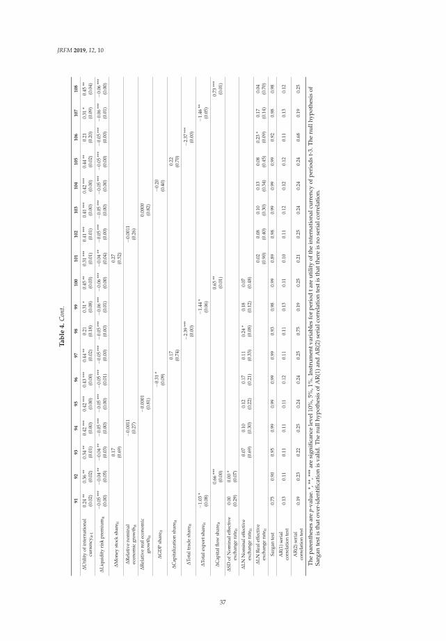
JRFM 2019, 12, 10
Ta
ble
4.
Con
t.
91
92
93
94
95
96
97
98
99
100
101
102
103
104
105
106
107
108
ΔU
tilit
yof
inte
rnat
iona
lcu
rren
cyit
-1
0.24
**0.
36**
0.34
**0.
42**
*0.
42**
*0.
43**
*0.
44**
0.21
0.31
*0.
45**
0.31
***
0.41
***
0.41
***
0.42
***
0.44
**0.
210.
31*
0.45
**(0
.02)
(0.0
2)(0
.01)
(0.0
0)(0
.00)
(0.0
0)(0
.02)
(0.1
8)(0
.08)
(0.0
3)(0
.01)
(0.0
1)(0
.00)
(0.0
0)(0
.02)
(0.2
0)(0
.09)
(0.0
4)
ΔLi
quid
ity
risk
prem
ium
it−0
.05
***
−0.0
4**
−0.0
4**
−0.0
5**
*−0
.05
***
−0.0
5**
*−0
.05
***
−0.0
5**
*−0
.06
***
−0.0
6**
*−0
.04
**−0
.05
***
−0.0
5**
*−0
.05
***
−0.0
5**
*−0
.05
***
−0.0
6**
*−0
.06
***
(0.0
0)(0
.05)
(0.0
3)(0
.00)
(0.0
0)(0
.01)
(0.0
0)(0
.00)
(0.0
1)(0
.00)
(0.0
4)(0
.00)
(0.0
0)(0
.00)
(0.0
0)(0
.00)
(0.0
1)(0
.00)
ΔM
oney
stoc
ksh
are i
t0.
170.
27(0
.69)
(0.5
2)
ΔR
elat
ive
nom
inal
econ
omic
grow
thit
−0.0
011
−0.0
011
(0.2
7)(0
.26)
ΔR
elat
ive
real
econ
omic
grow
thit
−0.0
001
0.00
00(0
.81)
(0.8
2)
ΔG
DP
shar
e it
−0.3
1*
−0.2
0(0
.09)
(0.4
0)
ΔC
apit
aliz
atio
nsh
are i
t0.
170.
22(0
.74)
(0.7
0)
ΔTo
talt
rade
shar
e it
−2.3
9**
*−2
.37
***
(0.0
0)(0
.00)
ΔTo
tale
xpor
tsha
reit
−1.0
3*
−1.4
4*
−1.4
6**
(0.0
8)(0
.06)
(0.0
5)
ΔC
apit
alflo
wsh
are i
t0.
66**
*0.
65**
0.73
***
(0.0
0)(0
.01)
(0.0
1)
ΔSD
ofN
omin
alef
fect
ive
exch
ange
rate
it
0.00
0.00
*(0
.29)
(0.0
7)
ΔLN
Nom
inal
effe
ctiv
eex
chan
gera
teit
0.07
0.10
0.12
0.17
0.11
0.24
*0.
180.
07(0
.69)
(0.3
0)(0
.22)
(0.2
1)(0
.33)
(0.0
8)(0
.12)
(0.4
8)
ΔLN
Rea
leff
ecti
veex
chan
gera
teit
0.02
0.08
0.10
0.13
0.08
0.23
*0.
170.
04(0
.90)
(0.4
0)(0
.30)
(0.3
4)(0
.45)
(0.0
9)(0
.14)
(0.7
0)
Sarg
ante
st0.
750.
900.
950.
990.
990.
990.
990.
930.
980.
990.
890.
980.
990.
990.
990.
920.
980.
98
AR
(1)s
eria
lco
rrel
atio
nte
st0.
130.
110.
110.
110.
110.
120.
110.
110.
130.
110.
100.
110.
120.
120.
120.
110.
130.
12
AR
(2)s
eria
lco
rrel
atio
nte
st0.
190.
230.
220.
250.
240.
240.
250.
750.
190.
250.
210.
250.
240.
240.
240.
680.
190.
25
The
pare
nthe
ses
are
p-va
lue.
*,**
,***
are
sign
ifica
nce
leve
l10%
,5%
,1%
.Ins
trum
entv
aria
bles
for
peri
odta
reut
ility
ofth
ein
tern
atio
nalc
urre
ncy
ofpe
riod
st-
3.Th
enu
llhy
poth
esis
ofSa
rgan
test
isth
atov
er-i
dent
ifica
tion
isva
lid.T
henu
llhy
poth
esis
ofA
R(1
)and
AR
(2)s
eria
lcor
rela
tion
test
isth
atth
ere
isno
seri
alco
rrel
atio
n.
37

JRFM 2019, 12, 10
Ta
ble
5.
Det
erm
inan
tsut
ility
ofin
tern
atio
nalc
urre
ncy
(rea
lint
eres
trat
e3.
0%).
109
110
111
112
113
114
115
116
117
118
119
120
121
122
123
124
125
126
ΔU
tilit
yof
inte
rnat
iona
lcu
rren
cyit
-1
−0.0
30.
06*
−0.0
20.
06**
0.03
0.14
0.05
0.16
−0.0
60.
05−0
.05
0.06
0.29
***
0.27
**0.
27**
0.30
***
0.30
***
0.17
***
(0.6
9)(0
.06)
(0.7
9)(0
.04)
(0.5
5)(0
.24)
(0.4
2)(0
.20)
(0.5
7)(0
.26)
(0.6
3)(0
.17)
(0.0
0)(0
.01)
(0.0
1)(0
.01)
(0.0
0)(0
.00)
ΔLi
quid
ity
risk
prem
ium
it−0
.02
−0.0
3−0
.02
−0.0
3−0
.03
−0.0
4−0
.03
−0.0
4−0
.03
−0.0
4−0
.03
−0.0
4−0
.02
−0.0
2−0
.02
−0.0
2−0
.02
−0.0
3(0
.42)
(0.3
3)(0
.42)
(0.3
3)(0
.29)
(0.2
5)(0
.28)
(0.2
4)(0
.38)
(0.2
9)(0
.37)
(0.2
8)(0
.41)
(0.2
8)(0
.33)
(0.3
2)(0
.31)
(0.1
4)
ΔM
oney
stoc
ksh
are i
t0.
360.
370.
380.
400.
240.
330.
280.
380.
200.
280.
220.
320.
31(0
.28)
(0.2
8)(0
.25)
(0.2
3)(0
.67)
(0.5
7)(0
.63)
(0.5
1)(0
.58)
(0.4
9)(0
.53)
(0.4
3)(0
.16)
ΔR
elat
ive
nom
inal
econ
omic
grow
thit
−0.0
003
−0.0
006
−0.0
003
−0.0
007
−0.0
002
−0.0
006
−0.0
009
(0.3
2)(0
.14)
(0.4
4)(0
.21)
(0.3
1)(0
.12)
(0.2
0)
ΔR
elat
ive
real
econ
omic
grow
thit
0.00
000.
0000
0.00
00−0
.000
10.
0000
0.00
00−0
.000
1(0
.99)
(0.9
0)(1
.00)
(0.8
0)(0
.94)
(0.8
8)(0
.79)
ΔG
DP
shar
e it
0.39
0.18
0.39
0.18
0.03
−0.1
90.
00−0
.22
0.27
0.05
0.27
0.04
0.23
(0.2
8)(0
.33)
(0.2
5)(0
.25)
(0.9
4)(0
.64)
(0.9
9)(0
.59)
(0.2
4)(0
.88)
(0.2
4)(0
.90)
(0.2
0)
ΔC
apit
aliz
atio
nsh
are i
t−0
.06
−0.2
0−0
.05
−0.1
70.
06−0
.09
0.07
−0.0
7−0
.02
−0.1
7−0
.02
−0.1
60.
17(0
.83)
(0.1
8)(0
.86)
(0.2
5)(0
.77)
(0.7
2)(0
.72)
(0.7
9)(0
.94)
(0.2
6)(0
.93)
(0.3
0)(0
.10)
ΔTo
talt
rade
shar
e it
−2.4
5**
*−2
.46
***
−2.4
0**
*−2
.39
***
−2.5
2**
*−2
.52
***
−1.4
1**
*(0
.00)
(0.0
0)(0
.00)
(0.0
0)(0
.00)
(0.0
0)(0
.00)
ΔTo
tale
xpor
tsha
reit
−1.7
8**
−1.8
1**
−1.6
5**
−1.6
5**
−1.8
0**
−1.8
2**
(0.0
2)(0
.02)
(0.0
1)(0
.02)
(0.0
1)(0
.02)
ΔC
apit
alflo
wsh
are i
t0.
530.
520.
520.
490.
650.
670.
640.
650.
570.
600.
560.
57(0
.28)
(0.3
8)(0
.30)
(0.4
2)(0
.19)
(0.2
3)(0
.20)
(0.2
6)(0
.39)
(0.4
1)(0
.41)
(0.4
5)
ΔSD
ofN
omin
alef
fect
ive
exch
ange
rate
it
0.00
0.00
0.00
0.00
0.00
0.00
0.00
0.00
0.00
0.00
(0.5
3)(0
.42)
(0.5
2)(0
.40)
(0.3
0)(0
.30)
(0.3
0)(0
.29)
(0.2
7)(0
.37)
ΔLN
Nom
inal
effe
ctiv
eex
chan
gera
teit
0.10
0.07
0.11
0.08
(0.2
3)(0
.38)
(0.2
2)(0
.35)
ΔLN
Rea
leff
ecti
veex
chan
gera
teit
0.07
0.04
0.07
0.05
(0.3
2)(0
.55)
(0.3
1)(0
.50)
Sarg
ante
st0.
290.
510.
320.
560.
480.
680.
550.
760.
250.
490.
290.
550.
860.
810.
830.
880.
870.
41
AR
(1)s
eria
lco
rrel
atio
nte
st0.
140.
130.
130.
130.
150.
180.
150.
180.
230.
170.
220.
170.
09*
0.12
0.12
0.10
*0.
110.
14
AR
(2)s
eria
lco
rrel
atio
nte
st0.
08*
0.15
0.08
*0.
150.
190.
130.
210.
130.
180.
120.
190.
110.
230.
220.
220.
230.
220.
17
38
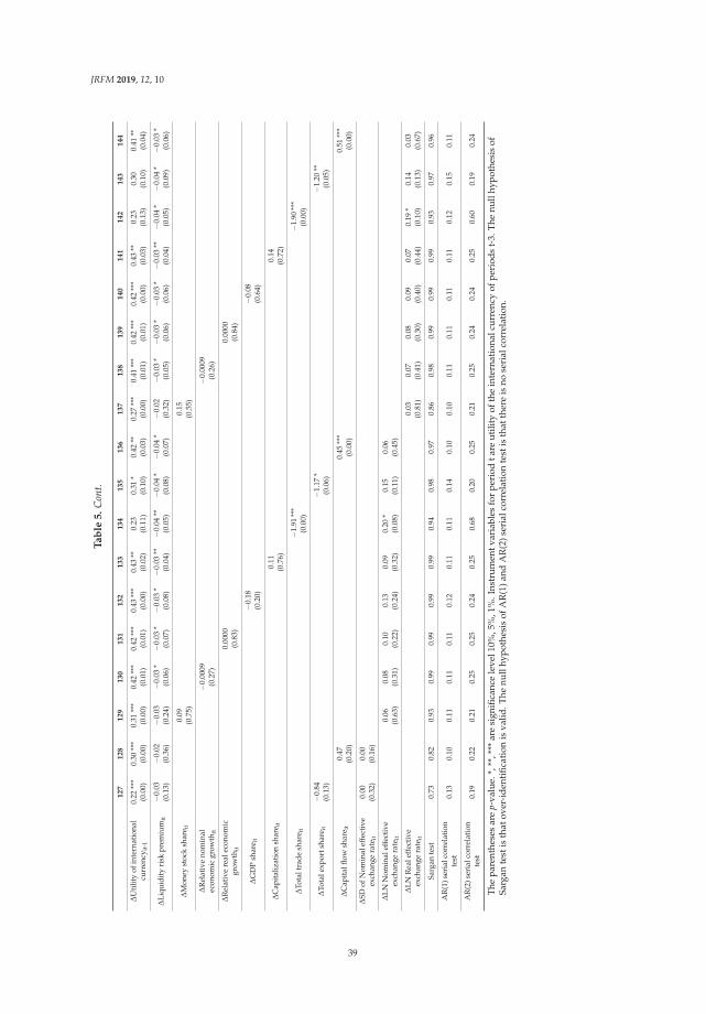
JRFM 2019, 12, 10
Ta
ble
5.
Con
t.
127
128
129
130
131
132
133
134
135
136
137
138
139
140
141
142
143
144
ΔU
tilit
yof
inte
rnat
iona
lcu
rren
cyit
-1
0.22
***
0.30
***
0.31
***
0.42
***
0.42
***
0.43
***
0.43
**0.
230.
31*
0.42
**0.
27**
*0.
41**
*0.
42**
*0.
42**
*0.
43**
0.23
0.30
0.41
**(0
.00)
(0.0
0)(0
.00)
(0.0
1)(0
.01)
(0.0
0)(0
.02)
(0.1
1)(0
.10)
(0.0
3)(0
.00)
(0.0
1)(0
.01)
(0.0
0)(0
.03)
(0.1
3)(0
.10)
(0.0
4)
ΔLi
quid
ity
risk
prem
ium
it−0
.03
−0.0
2−0
.03
−0.0
3*
−0.0
3*
−0.0
3*
−0.0
3**
−0.0
4**
−0.0
4*
−0.0
4*
−0.0
2−0
.03
*−0
.03
*−0
.03
*−0
.03
**−0
.04
*−0
.04
*−0
.03
*(0
.13)
(0.3
6)(0
.24)
(0.0
6)(0
.07)
(0.0
8)(0
.04)
(0.0
5)(0
.08)
(0.0
7)(0
.32)
(0.0
5)(0
.06)
(0.0
6)(0
.04)
(0.0
5)(0
.09)
(0.0
6)
ΔM
oney
stoc
ksh
are i
t0.
090.
15(0
.75)
(0.5
5)
ΔR
elat
ive
nom
inal
econ
omic
grow
thit
−0.0
009
−0.0
009
(0.2
7)(0
.26)
ΔR
elat
ive
real
econ
omic
grow
thit
0.00
000.
0000
(0.8
3)(0
.84)
ΔG
DP
shar
e it
−0.1
8−0
.08
(0.2
0)(0
.64)
ΔC
apit
aliz
atio
nsh
are i
t0.
110.
14(0
.76)
(0.7
2)
ΔTo
talt
rade
shar
e it
−1.9
1**
*−1
.90
***
(0.0
0)(0
.00)
ΔTo
tale
xpor
tsha
reit
−0.8
4−1
.17
*−1
.20
**(0
.13)
(0.0
6)(0
.05)
ΔC
apit
alflo
wsh
are i
t0.
470.
45**
*0.
51**
*(0
.20)
(0.0
0)(0
.00)
ΔSD
ofN
omin
alef
fect
ive
exch
ange
rate
it
0.00
0.00
(0.3
2)(0
.16)
ΔLN
Nom
inal
effe
ctiv
eex
chan
gera
teit
0.06
0.08
0.10
0.13
0.09
0.20
*0.
150.
06(0
.63)
(0.3
1)(0
.22)
(0.2
4)(0
.32)
(0.0
8)(0
.11)
(0.4
5)
ΔLN
Rea
leff
ecti
veex
chan
gera
teit
0.03
0.07
0.08
0.09
0.07
0.19
*0.
140.
03(0
.81)
(0.4
1)(0
.30)
(0.4
0)(0
.44)
(0.1
0)(0
.13)
(0.6
7)
Sarg
ante
st0.
730.
820.
930.
990.
990.
990.
990.
940.
980.
970.
860.
980.
990.
990.
990.
930.
970.
96
AR
(1)s
eria
lcor
rela
tion
test
0.13
0.10
0.11
0.11
0.11
0.12
0.11
0.11
0.14
0.10
0.10
0.11
0.11
0.11
0.11
0.12
0.15
0.11
AR
(2)s
eria
lcor
rela
tion
test
0.19
0.22
0.21
0.25
0.25
0.24
0.25
0.68
0.20
0.25
0.21
0.25
0.24
0.24
0.25
0.60
0.19
0.24
The
pare
nthe
ses
are
p-va
lue.
*,**
,***
are
sign
ifica
nce
leve
l10%
,5%
,1%
.Ins
trum
entv
aria
bles
for
peri
odta
reut
ility
ofth
ein
tern
atio
nalc
urre
ncy
ofpe
riod
st-
3.Th
enu
llhy
poth
esis
ofSa
rgan
test
isth
atov
er-i
dent
ifica
tion
isva
lid.T
henu
llhy
poth
esis
ofA
R(1
)and
AR
(2)s
eria
lcor
rela
tion
test
isth
atth
ere
isno
seri
alco
rrel
atio
n.
39
JRFM 2019, 12, 10
7. Conclusions
In this paper, we investigated what determines utility of the international currencies among thecurrent major currencies which include the US dollar, the euro, the Japanese yen, and the Britishpound. We used a dynamic panel data model to analyze the issue with GMM. We focused on effects ofliquidity shortage in terms of an international currency on utility of the international currencies aswell as inertia of the US dollar as the key currency. We made empirical analysis of whether liquidityrisk premium in an international currency as well as other possible determinant factors affect utility ofthe relevant international currency.
We obtained the following results from the empirical analysis. Firstly, change in utility of theinternational currency in the previous period has significantly a positive effect on the change of utilityof the international currency in the current period. This suggests that utility of the internationalcurrency tends to fluctuate in the same direction as the change in the previous term. For example, if theutility of the international currency decreases, we assumed that the currency is less likely to be usedthan in the previous period, which will continue in the next period. Secondly, the change of liquidityrisk premium has significantly a negative effect on the change of utility of the currency. This suggeststhat liquidity shortage reduce the utility of the international currency. Thirdly, the change of capitalflow share has significantly a positive effect on the change of utility of the international currency. Thissuggests that increase in economic scale may increase utility of the international currency.
We mention policy implications from the empirical results. As mentioned above, liquidity riskpremium and capital flow had influence on utility of the international currency. If the monetary authoritiestry to internationalize their home currencies, it is necessary to focus on these variables. It is consideredthat utility of the international currency will increase by conducting policies that increase liquidity ofthe currency or increase international capital flows. It might be possible to push internationalization ofthe home currencies through this increase of utility of the international currencies.
Moreover, in this analysis, we found a strong relationship between utility of the internationalcurrency and liquidity of the international currency. We should also deeply analyze relationshipbetween the two variables. In this analysis, as we supposed that utility of the international currencyis dependent variable, changes in liquidity of the international currency have influenced changes inthe utility of the international currency. However, it is necessary for us to suppose causality betweenthe liquidity of the international currency and its utility in the opposite direction. If utility of aninternational currency declines, it may reduce liquidity of the international currency through reductionin convenience of the currency.
We used liquidity risk premium as a variable for liquidity of the international currency in thispaper. There are such other variables as bid-ask spreads that represent liquidity of the internationalcurrency. Moreover, it is capital adequacy of financial institution that could affect liquidity of theinternational currency. It is necessary to conduct robustness tests for the analysis result by conductingany analysis using the variables in the future. Furthermore, we used ARIMA model using CPI for theexpected inflation rate. Other expected inflation rate data include TIPS data and survey data, whichmay reflect the reality. Robustness check using these data as future work is also necessary.
In addition, we have further study regarding what factors are important to help an emerging newinternational currency which includes the Chinese yuan. In recent years, the Chinese governmenthas been promoting the Chinese yuan to be internationalized while the IMF has added it into majorinternational currencies that is component currencies of the Special Drawing Rights (SDR). It isimportant for us to investigate how a local currency can emerge as an international currency and,in turn, make it into a key currency in the current international monetary system where we do not as arule set any currencies as a key currency.
Author Contributions: Conceptualization, E.O.; methodology, E.O.; formal analysis, M.M.; investigation, M.M.;writing—original draft preparation, E.O. and M.M.; writing—review and editing, E.O. and M.M.; visualization,E.O. and M.M.; supervision, E.O.; project administration, E.O.
40
JRFM 2019, 12, 10
Funding: This research received no external funding.
Acknowledgments: This study is conducted as a part of the project “Exchange Rate and International Currency”undertaken at the Research Institute of Economy, Trade and Industry (RIETI). The authors are grateful to the threeanonymous referees, Keiichiro Kobayashi, Etsuro Shioji, Shinichi Fukuda, Jorg Mayer, Stephan Gerlach and otherparticipants in the RIETI research seminar, a research meeting of the Ministry of Finance, and conferences of theAsia-Pacific Economic Association and Japan Economic Network for their useful comments and suggestions.
Conflicts of Interest: The authors declare no conflict of interest.
Appendix A. Derivation of Equation (1)
We base on a Sidrauski (1967)-type of money-in-the-utility model in which real balances of money aswell as consumption are supposed as explanatory variables in a utility function. According to Ogawa andSasaki (1998), we extend the money-in-the-utility model to a dynamic one with parallel internationalcurrencies5. We suppose that the international currencies are held by private economic agents in a thirdcountry. For simplicity, we suppose that two monetary authorities supply international currencies.
For convenience, we suppose that it is both the monetary authorities in the Country i andother countries O that supply their international currencies. The monetary authorities in Country isupply currency i while the monetary authorities in other countries O supply their own currenciesO. The private sector in the third country A is able to use both the currencies i and O as internationalcurrencies in international economic transactions. The monetary authorities in country A adopt aflexible exchange rate system.
We suppose a situation that bonds in currencies i and O are available to the private sector incountry A and that no bonds denominated in currency A are issued in country A. We assume perfectcapital mobility and perfect substitution for the bonds of different currencies. Moreover, we assumethat the private sector has perfect foresight. Thus, uncovered interest parity holds in the model. On onehand, we assume perfect flexible prices and a law of one price. Thus, the purchasing power parityalways holds in the model. For simplicity, we assume that its rate of time preference is constant overtime and is equal to a real interest rate. Given the assumptions, the real interest rate is constant overtime. Real interest rates in all countries are equal to each other by both the uncovered interest parityand purchasing power parity.
The private sector in country A holds home currency A, international currencies i and O, and bondsin currencies i and O. Instantaneous budget constraints for the private sector are represented inreal terms:
.wp
t = rwpt + yt − ct − τt − iA
t mAt − ii
tmit − iOt mO
t (A1a)
wpt = bi
t + bOt + mA
t + mit + mO
t (A1b)
where y: real gross domestic products, τ: real taxes, c: real consumption, ij: nominal interest rate incurrency j (j = A, i, O), wp: real balance of financial assets held by the private sector, mj: real balance ofhome currency j(j = A, i, O) held by the private sector, bj: real balance of bond in currency j (j = i, O)held by the private sector, r: real interest rate. A dot over variables implies a change in the relevantvariables. We assume no-Ponzi game conditions for the real balance of financial assets held by theprivate sector (wp).
limt→∞
wpt e−rt ≥ 0 (A2)
We assume that the private sector maximizes its utility over an infinite horizon subject to budgetconstraints (A1a) and (A1b). We specify a Cobb-Douglas type of instantaneous utility function:∫ ∞
0U(ct, mA
t , mit, mO
t )e−δtdt (A3a)
5 See Ogawa and Muto (2017a) for the detailed derivation.
41

JRFM 2019, 12, 10
U(ct, mAt , mi
t, mOt ) ≡
[cα
t
{mAβ
t
(miγ
t mO1−γ
t
)1−β}1−α
]1−R
1 − R(A3b)
0 < α < 1, 0 < β < 1, 0 < γ < 1, 0 < R < 1
where δ: rate of time preference, R: reciprocal of instantaneous elasticity of substitution betweenintertemporal consumption σ: σ ≡ − Uc
UccctWe assume that the public sector in country A holds only bonds in currencies i and O.
Instantaneous budget constraints for the public sector are represented in real terms:
.f t = r ft + τt + μA
t mAt − gt (A4a)
ft ≡ f it + f O
t (A4b)
where g: real government expenditures, f : foreign assets held by the public sector, μA: growth rate ofcurrency A. We assume no-Ponzi game conditions for foreign assets held by the public sector.
limt→∞
fte−rt ≥ 0 (A5)
A stock of foreign exchange reserves held by the monetary authorities should be unchangedunder a flexible exchange rate system because the monetary authorities will not intervene in foreignexchange markets ( ft = f ). Also, they are able to control nominal money supply. Here, we assumethat they increase the nominal money supply at a constant growth rate μA.
Thus we obtain an instantaneous budget constraint equation for the public sector under a flexibleexchange rate system:
gt − τt = r f + μAmAt (A6)
From the instantaneous budget constraint equations for the private sector and the public sectorEquations (A1a) and (A6), we derive an instantaneous budget constraint equation for the wholeeconomy of country A under a flexible exchange rate system:
.b
it +
.b
Ot +
.mi
t +.
mOt = r(bi
t + bOt + mi
t + mit + f ) + yt − ct − gt − ii
tmit − iOt mO
t (A7)
The private sector maximizes its utility Functions (A3a) and (A3b) subject to budget constraintEquation (A7). We assume that the private sector has perfect foresight that economic variables do notdiverge to infinity but converge to equilibrium values along a saddle path to rule out a possibility ofmultiplicity of equilibria in the model.
From the first-order conditions for maximization, we derive optimal real balances of internationalcurrencies:
mit =
(1 − α)(1 − β)γ
α
ciit=
(1 − α)(1 − β)γ
α
ciit + r
(A8a)
mOt =
(1 − α)(1 − β)(1 − γ)
α
ciOt
=(1 − α)(1 − β)(1 − γ)
α
ciOt + r
(A8b)
where πjt: inflation rate of currency j(j = i, O),
c = r
⎧⎨⎩a0 +
∞∫0
yte−rtdt −∞∫
0
gte−rtdt−∞∫
0
(iitm
it − iOt mO
t )e−rtdt
⎫⎬⎭
42

JRFM 2019, 12, 10
From Equations (A8a) and (A8b), an optimal share φ of i is derived:
φt ≡ mit
mit + mO
t=
1
1 + 1−γγ
iitiOt
=1
1 + 1−γγ
πit+r
πOt +r
(A9)
Equation (A9) implies that the optimal share of i depends on both the inflation or depreciation ratesof the international currencies (πi and πO) and a parameter γ in the utility function Equation (A3b).
From Equation (A9), the parameter γit is derived:
γit =
1
1 +(
1φi
t− 1)
πOt +r
πit+r
(A10)
References
Arellano, Manuel, and Stephen Bond. 1991. Some Tests of Specification for Panel Data: Monte Carlo Evidence andan Application to Employment Equations. The Review of Economic Studies 58: 277–97. [CrossRef]
Blanchard, Olivier J., and Stanley Fischer. 1989. Lectures on Macroeconomics. Cambridge: MIT Press.Calvo, Guillermo A. 1981. Devaluation: Levels versus Rates. Journal of International Economics 11: 165–72. [CrossRef]Calvo, Guillermo A. 1985. Currency Substitution and the Real Exchange Rate: The Utility Maximization Approach.
Journal of International Money and Finance 4: 175–88. [CrossRef]Catão, Luis, and Marco Terrones. 2016. Financial De-Dollarization—A Global Perspective and the Peruvian Experience.
IMF Working Paper WP/16/97. Washington, DC: International Monetary Fund. [CrossRef]Chinn, Menzie, and Jeffrey A. Frankel. 2007. Will the Euro Eventually Surpass the Dollar as Leading International
Reserve Currency? In G7 Current Account Imbalances: Sustainability and Adjustment. Edited by Richard H. Clarida.Chicago: University of Chicago Press, pp. 283–338.
Chinn, Menzie, and Jeffrey A. Frankel. 2008. Why the Euro Will Rival the Dollar. International Finance 11: 49–73.[CrossRef]
Eichengreen, Barry, Livia Chitu, and Arnaud Mehl. 2016a. Network Effects, Homogeneous Goods andInternational Currency Choice: New Evidence on Oil Markets from an Older Era. Canadian Journal ofEconomics/Revue Canadienne d’économique 49: 173–206. [CrossRef]
Eichengreen, Barry, Livia Chitu, and Arnaud Mehl. 2016b. Stability or Upheaval? The Currency Composition ofInternational Reserves in the Long Run. IMF Economic Review 64: 354–80. [CrossRef]
European Central Bank. 2015. The International Role of the Euro. Frankfurt: European Central Bank.Fama, Eugene F., and Michael R. Gibbons. 1984. A Comparison of Inflation Forecasts. Journal of Monetary Economics
13: 327–48. [CrossRef]Goldberg, Linda S., and Cédric Tille. 2008. Vehicle Currency Use in International Trade. Journal of International
Economics 76: 177–92. [CrossRef]Honohan, Patrick. 2008. The Retreat of Deposit Dollarization. International Finance 11: 247–68. [CrossRef]Ito, Takatoshi, Satoshi Koibuchi, Kiyotaka Sato, and Junko Shimizu. 2013. Choice of Invoicing Currency: New
Evidence from a Questionnaire Survey of Japanese Export Firms. Discussion Paper. Research Instituteof Economy, Trade and Industry (RIETI) Discussion Paper Series, No. 13-E-034. Available online: https://econpapers.repec.org/paper/etidpaper/13034.htm (accessed on 7 January 2019).
Kamps, Annette. 2006. The Euro as Invoicing Currency in International Trade (August 2006). ECB Working PaperNo. 665. Available online: https://papers.ssrn.com/abstract=926402 (accessed on 7 January 2019).
Kannan, Prakash. 2009. On the Welfare Benefits of an International Currency. European Economic Review 53: 588–606.[CrossRef]
Krugman, Paul R. 1984. The International Role of the Dollar: Theory and Prospect. In Exchange Rate Theory andPractice. Chicago: University of Chicago Press, pp. 261–78.
Matsuyama, Kiminori, Nobuhiro Kiyotaki, and Akihiko Matsui. 1993. Toward a Theory of International Currency.The Review of Economic Studies 60: 283–307. [CrossRef]
Obstfeld, Maurice. 1981. Macroeconomic Policy, Exchange-Rate Dynamics, and Optimal Asset Accumulation.Journal of Political Economy 89: 1142–61. [CrossRef]
43

JRFM 2019, 12, 10
Ogawa, Eiji, and Makoto Muto. 2017a. Inertia of the US Dollar as a Key Currency Through the Two Crises.Emerging Markets Finance and Trade 53: 2706–24. [CrossRef]
Ogawa, Eiji, and Makoto Muto. 2017b. Declining Japanese Yen in the Changing International Monetary System.East Asian Economic Review 21: 317–42. [CrossRef]
Ogawa, Eiji, and Yuri Nagataki Sasaki. 1998. Inertia in the Key Currency. Japan and The World Economy 10: 421–39.[CrossRef]
Sidrauski, Miguel. 1967. Rational Choice and Patterns of Growth in a Monetary Economy. The American EconomicReview 57: 534–44.
Trejos, Alberto, and Randall Wright. 1996. Search—Theoretic Models of International Currency. Review 78.[CrossRef]
© 2019 by the authors. Licensee MDPI, Basel, Switzerland. This article is an open accessarticle distributed under the terms and conditions of the Creative Commons Attribution(CC BY) license (http://creativecommons.org/licenses/by/4.0/).
44
Journal of
Risk and FinancialManagement
Article
Can We Forecast Daily Oil Futures Prices?Experimental Evidence from ConvolutionalNeural Networks
Zhaojie Luo 1 , Xiaojing Cai 2, Katsuyuki Tanaka 2, Tetsuya Takiguchi 1,*, Takuji Kinkyo 2 and
Shigeyuki Hamori 2
1 Graduate School of System Informatics, Kobe University, 2-1 Rokkodai, Nada-Ku, Kobe 657-8501, Japan;[email protected]
2 Graduate School of Economics, Kobe University, 2-1 Rokkodai, Nada-Ku, Kobe 657-8501, Japan;[email protected] (X.C.); [email protected] (K.T.); [email protected] (T.K.);[email protected] (S.H.)
* Correspondence: [email protected]
Received: 21 November 2018; Accepted: 2 January 2019; Published: 8 January 2019
Abstract: This paper proposes a novel approach, based on convolutional neural network (CNN)models, that forecasts the short-term crude oil futures prices with good performance. In ourstudy, we confirm that artificial intelligence (AI)-based deep-learning approaches can providemore accurate forecasts of short-term oil prices than those of the benchmark Naive Forecast(NF) model. We also provide strong evidence that CNN models with matrix inputs are betterat short-term prediction than neural network (NN) models with single-vector input, which indicatesthat strengthening the dependence of inputs and providing more useful information can improveshort-term forecasting performance.
Keywords: crude oil futures prices forecasting; convolutional neural networks; short-term forecasting
1. Introduction
Crude oil is a vital fuel, accounting for 32.9% of global energy consumption in 2016 accordingto BP’s Statistical Energy Outlook, which indicates that crude oil will continue to play an importantrole until 2035. It is fair to argue that the movement in the crude oil price should have a significanteffect on macroeconomic aggregates, such as the GDP and inflation of oil-exporting and -importingcountries. On the other hand, as one of the most actively traded commodities in the world(Alvarez-Ramirez et al. (2012)), crude oil futures have become an important financial asset and anadditional investment tool. Owing to the increasing correlation between traditional financial markets,such as stocks, bonds, and foreign exchange, international investors are searching for new investmenttools, such as crude oil futures, to enhance returns, diversify portfolios, and hedge against inflation.Therefore, forecasting oil futures prices accurately is crucial and helps international investors todiversify risk.
Many researchers have proposed and developed economic models to forecast crude oil spotprices (De Souza e Silva et al. (2010); Ye et al. (2006); Merino and Ortiz (2005); Wang et al. (2016);Wen et al. (2016); Baumeister et al. (2015); Naser (2016)). However, studies forecasting futures prices arescarce. According to Sklibosios Nikitopoulos et al. (2017), futures prices depend on the value of deferreduse. For example, decreasing futures prices show that the value of immediate use (consumption) orthe yield to holders of physical inventory is reducing. Therefore, futures prices are vulnerable to manycomplex natural, economic, and political factors, such as the economic development conditions of oilgiants, oil wars, international petroleum organizations and so on. A large number of these factors are
JRFM 2019, 12, 9; doi:10.3390/jrfm12010009 www.mdpi.com/journal/jrfm45

JRFM 2019, 12, 9
random, resulting in sharp fluctuations in the crude oil futures markets and showing very complexnonlinear characteristics. Thus, it is difficult to predict the futures prices accurately.
Recently, as new technologies are developed, artificial intelligence (AI) techniques (e.g., neuralnetworks (NNs)) have been applied to the prediction of time series. AI-based models emulatethe human brain to provide feedback on large quantities of data, and to learn to recognizeinformation patterns. Thus, NN models can create a breakthrough opportunity in the analysis ofthe non-linear behavior of the time series of the crude oil markets (Refenes (1994); Ongkrutaraksa(1995); Moshiri and Foroutan (2006); Jammazi and Aloui (2012); Mingming and Jinliang (2012); Wanget al. (2005)). For example, Moshiri and Foroutan (2006) compared linear (Autoregressive movingaverage models and Generalized autoregressive conditional heteroscedasticity models) and nonlinearNN models, and found that NNs are superior and produce a more statistically significant forecast.Jammazi and Aloui (2012) combined the wavelet transform and NNs to forecast the crude oil monthlyprice. Mingming and Jinliang (2012) constructed a multiple-wavelet recurrent NN model to analyzecrude oil monthly prices. Wang et al. (2005) present an NN-based model to forecast crude oil monthlyprices, and claimed superior performance by their model. These results prove that an AI-basedforecasting model can provide greater efficiency and higher accuracy than other models.
Here, we propose a novel, deep-learning forecasting approach based on a convolutional neuralnetworks (CNNs) model for short-term1 forecasting using daily data of crude oil futures prices.Unlike NNs with a single-vector neuron, the layers of the CNN model have neurons arranged in twodimensions (width and height). The CNNs take advantage of the fact that the inputs consist of matrices,which can strengthen the dependence and connections between neurons and constrain the architecturein a more sensible way. Moreover, instead of all the neurons in NNs being fully connected, the neuronsof the CNN in a layer are only connected to a small region of the previous layer, which enables CNNmodels to share connections among neurons more flexibly. These characteristics may improve theshort-term forecasting of crude oil prices. CNNs have recently been applied to large-scale image andvideo recognition (Krizhevsky et al. (2012); Zeiler and Fergus (2014); Simonyan and Zisserman (2014))and traffic-speed prediction (Ma et al. (2017)). To the best of our knowledge, our study is the firstCNN approach applied in the economic and financial field, and particularly to crude oil futures pricesforecasting. CNN models are used in modeling problems related to spatial inputs like images. They arenot suitable for processing and predicting events at relatively long intervals and delays in the timeseries. However, in our forecasting task, we used the daily oil prices to predict a short-term futureprice. Thus, CNN is suitable for this task due to its ability to capture the relevant features from thenearby daily prices in an image (one-week daily prices matrix). In addition, we normalized our data toovercome non-stationary time series and focus on the short-term oil futures prices trends using thedaily data. We employ CNN models to forecast crude oil daily prices, which has become possibleowing to the large daily data set.
Our study offers two contributions to the literature. First, we confirm that the non-lineardeep-learning approaches perform better for short-term forecasting by comparing AI-baseddeep-learning methods with the naive forecast (NF) and Autoregressive-Generalized autoregressiveconditional heteroscedasticity (AR-GARCH) model as two benchmarks, in terms of the accuracyof the short-term crude oil price forecasting. Second, we find that strengthening the dependenceof inputs and providing more useful information connections between neurons can improve theshort-term forecasting performance. Here we show that the CNN models are more powerful than thebenchmark models.
The remainder of this paper is organized as follows. In Section 2, we introduce our related workin technology. In Section 3, we describe the model specifications. We show our data and empiricalresults in Sections 4 and 5. Finally, our concluding remarks are presented in Section 6.
1 In this paper, the short-term forecast means the next day forecast that is the forecast is 1-step-ahead.
46
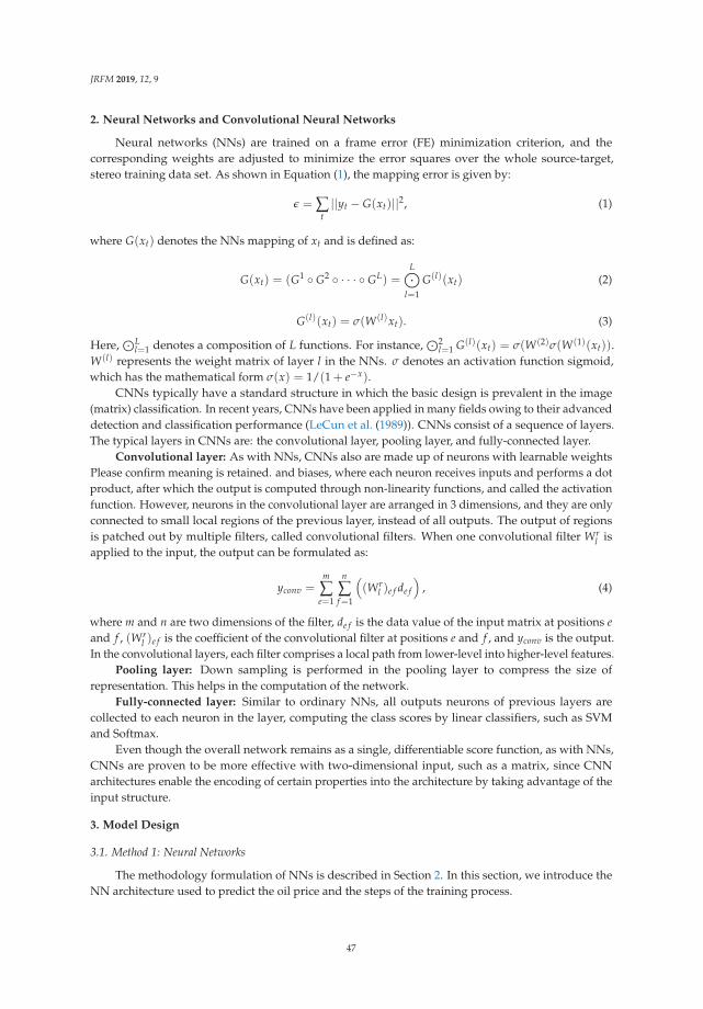
JRFM 2019, 12, 9
2. Neural Networks and Convolutional Neural Networks
Neural networks (NNs) are trained on a frame error (FE) minimization criterion, and thecorresponding weights are adjusted to minimize the error squares over the whole source-target,stereo training data set. As shown in Equation (1), the mapping error is given by:
ε = ∑t||yt − G(xt)||2, (1)
where G(xt) denotes the NNs mapping of xt and is defined as:
G(xt) = (G1 ◦ G2 ◦ · · · ◦ GL) =L⊙
l=1
G(l)(xt) (2)
G(l)(xt) = σ(W(l)xt). (3)
Here,⊙L
l=1 denotes a composition of L functions. For instance,⊙2
l=1 G(l)(xt) = σ(W(2)σ(W(1)(xt)).W(l) represents the weight matrix of layer l in the NNs. σ denotes an activation function sigmoid,which has the mathematical form σ(x) = 1/(1 + e−x).
CNNs typically have a standard structure in which the basic design is prevalent in the image(matrix) classification. In recent years, CNNs have been applied in many fields owing to their advanceddetection and classification performance (LeCun et al. (1989)). CNNs consist of a sequence of layers.The typical layers in CNNs are: the convolutional layer, pooling layer, and fully-connected layer.
Convolutional layer: As with NNs, CNNs also are made up of neurons with learnable weightsPlease confirm meaning is retained. and biases, where each neuron receives inputs and performs a dotproduct, after which the output is computed through non-linearity functions, and called the activationfunction. However, neurons in the convolutional layer are arranged in 3 dimensions, and they are onlyconnected to small local regions of the previous layer, instead of all outputs. The output of regionsis patched out by multiple filters, called convolutional filters. When one convolutional filter Wr
l isapplied to the input, the output can be formulated as:
yconv =m
∑e=1
n
∑f=1
((Wr
l )e f de f
), (4)
where m and n are two dimensions of the filter, de f is the data value of the input matrix at positions eand f , (Wr
l )e f is the coefficient of the convolutional filter at positions e and f , and yconv is the output.In the convolutional layers, each filter comprises a local path from lower-level into higher-level features.
Pooling layer: Down sampling is performed in the pooling layer to compress the size ofrepresentation. This helps in the computation of the network.
Fully-connected layer: Similar to ordinary NNs, all outputs neurons of previous layers arecollected to each neuron in the layer, computing the class scores by linear classifiers, such as SVMand Softmax.
Even though the overall network remains as a single, differentiable score function, as with NNs,CNNs are proven to be more effective with two-dimensional input, such as a matrix, since CNNarchitectures enable the encoding of certain properties into the architecture by taking advantage of theinput structure.
3. Model Design
3.1. Method 1: Neural Networks
The methodology formulation of NNs is described in Section 2. In this section, we introduce theNN architecture used to predict the oil price and the steps of the training process.
47
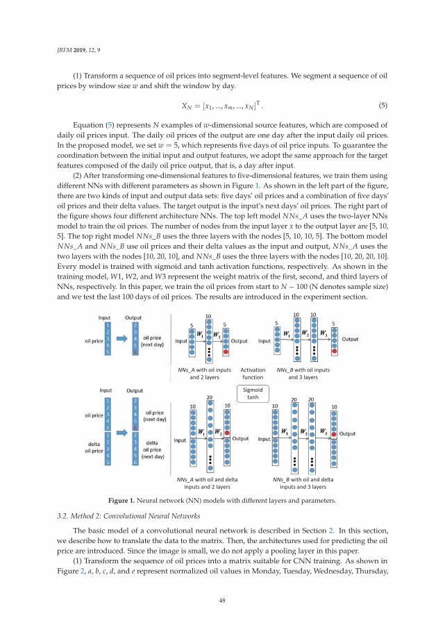
JRFM 2019, 12, 9
(1) Transform a sequence of oil prices into segment-level features. We segment a sequence of oilprices by window size w and shift the window by day.
XN = [x1, ..., xm, ..., xN ]T . (5)
Equation (5) represents N examples of w-dimensional source features, which are composed ofdaily oil prices input. The daily oil prices of the output are one day after the input daily oil prices.In the proposed model, we set w = 5, which represents five days of oil price inputs. To guarantee thecoordination between the initial input and output features, we adopt the same approach for the targetfeatures composed of the daily oil price output, that is, a day after input.
(2) After transforming one-dimensional features to five-dimensional features, we train them usingdifferent NNs with different parameters as shown in Figure 1. As shown in the left part of the figure,there are two kinds of input and output data sets: five days’ oil prices and a combination of five days’oil prices and their delta values. The target output is the input’s next days’ oil prices. The right part ofthe figure shows four different architecture NNs. The top left model NNs_A uses the two-layer NNsmodel to train the oil prices. The number of nodes from the input layer x to the output layer are [5, 10,5]. The top right model NNs_B uses the three layers with the nodes [5, 10, 10, 5]. The bottom modelNNs_A and NNs_B use oil prices and their delta values as the input and output, NNs_A uses thetwo layers with the nodes [10, 20, 10], and NNs_B uses the three layers with the nodes [10, 20, 20, 10].Every model is trained with sigmoid and tanh activation functions, respectively. As shown in thetraining model, W1, W2, and W3 represent the weight matrix of the first, second, and third layers ofNNs, respectively. In this paper, we train the oil prices from start to N − 100 (N denotes sample size)and we test the last 100 days of oil prices. The results are introduced in the experiment section.
Figure 1. Neural network (NN) models with different layers and parameters.
3.2. Method 2: Convolutional Neural Networks
The basic model of a convolutional neural network is described in Section 2. In this section,we describe how to translate the data to the matrix. Then, the architectures used for predicting the oilprice are introduced. Since the image is small, we do not apply a pooling layer in this paper.
(1) Transform the sequence of oil prices into a matrix suitable for CNN training. As shown inFigure 2, a, b, c, d, and e represent normalized oil values in Monday, Tuesday, Wednesday, Thursday,
48
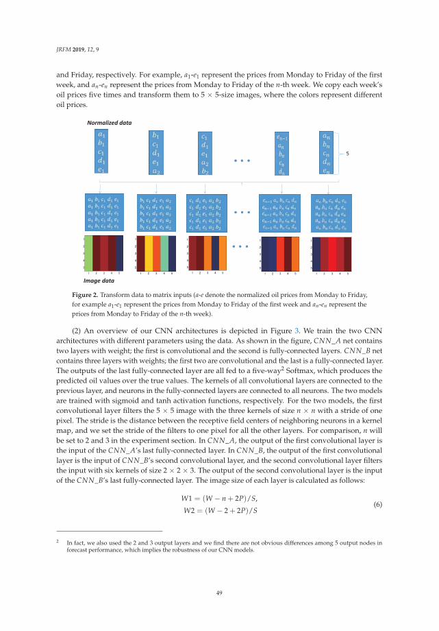
JRFM 2019, 12, 9
and Friday, respectively. For example, a1-e1 represent the prices from Monday to Friday of the firstweek, and an-en represent the prices from Monday to Friday of the n-th week. We copy each week’soil prices five times and transform them to 5 × 5-size images, where the colors represent differentoil prices.
Figure 2. Transform data to matrix inputs (a-e denote the normalized oil prices from Monday to Friday,for example a1-e1 represent the prices from Monday to Friday of the first week and an-en represent theprices from Monday to Friday of the n-th week).
(2) An overview of our CNN architectures is depicted in Figure 3. We train the two CNNarchitectures with different parameters using the data. As shown in the figure, CNN_A net containstwo layers with weight; the first is convolutional and the second is fully-connected layers. CNN_B netcontains three layers with weights; the first two are convolutional and the last is a fully-connected layer.The outputs of the last fully-connected layer are all fed to a five-way2 Softmax, which produces thepredicted oil values over the true values. The kernels of all convolutional layers are connected to theprevious layer, and neurons in the fully-connected layers are connected to all neurons. The two modelsare trained with sigmoid and tanh activation functions, respectively. For the two models, the firstconvolutional layer filters the 5 × 5 image with the three kernels of size n × n with a stride of onepixel. The stride is the distance between the receptive field centers of neighboring neurons in a kernelmap, and we set the stride of the filters to one pixel for all the other layers. For comparison, n willbe set to 2 and 3 in the experiment section. In CNN_A, the output of the first convolutional layer isthe input of the CNN_A’s last fully-connected layer. In CNN_B, the output of the first convolutionallayer is the input of CNN_B’s second convolutional layer, and the second convolutional layer filtersthe input with six kernels of size 2 × 2 × 3. The output of the second convolutional layer is the inputof the CNN_B’s last fully-connected layer. The image size of each layer is calculated as follows:
W1 = (W − n + 2P)/S,
W2 = (W − 2 + 2P)/S(6)
2 In fact, we also used the 2 and 3 output layers and we find there are not obvious differences among 5 output nodes inforecast performance, which implies the robustness of our CNN models.
49

JRFM 2019, 12, 9
W is the input image size. S is the stride with which we slide the filter. When the stride is 1, we movethe filters one pixel at a time. When the stride is 2, then the filters jump two pixels at a time as weslide them around. P represents the zero-padding, which pads the input volume with zeros aroundthe border. As described above, n is the kernel size. In this case, the input image is 5 × 5, so W is 5,the stride S is set to 1, and no zero-padding is P = 0. W1 and W2 represent the image size after theconvolutional processing. When training the CNN models, we used the Adam optimizer Kingma andBa (2014) with a mini-batch size of 20. The learning rate was set to 0.01, and the momentum term wasset to 0.1.
Figure 3. Train the 5 × 5-size economic data images by two different architectures. Convolutionalneural network (CNN). CNN_A (top): two-layers model with one convolutional layer and onefully-connected layer. CNN_B (bottom): three-layers model with two convolutional layers and onefully-connected layer.
4. Data
In this study, we use the daily Brent crude oil generic series of the first month’s futuresprices, traded on the Intercontinental Exchange (ICE). The data cover the period from 24 June 1988,to 3 November 2018, consisting of 7942 observations. The data were obtained from Bloomberg.
For training neural networks, data normalization is an effective way to obtain better performanceand quick convergence. Usually, we subtract the mean value to make the input mean zero to preventweights changing in the same directions, which is called the zero-mean normalization method.
The values of attribute X are normalized using the mean and standard deviation of X. A newvalue Xn is obtained using the following expression:
Xn =(X − Ux)
Sx, (7)
where Ux and Sx are the mean and standard deviation of attribute X, respectively. If Ux and Sx arenot known, they can be estimated from the samples. After zero-mean normalizing, each feature willhave a mean value of 0. In addition, the unit of each value will be the number of (estimated) standarddeviations away from the (estimated) mean. When zero-mean normalization is applied, all data ineach profile are slid vertically so that their average is zero. In most neural networks, they normalizethe data by the mean of all data. As shown in Figure 4, the middle curve is obtained from the top oneby a vertical translation so that the average of the profile is zero. Our method draws its strength frommaking normalization a part of the model architecture and performing the normalization for differenttraining segmentation using the following formula:
n = Numl(X)/k (8)
50
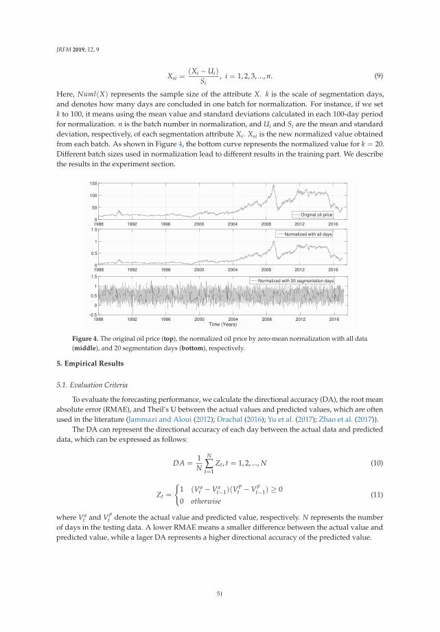
JRFM 2019, 12, 9
Xsi =(Xi − Ui)
Si, i = 1, 2, 3, ..., n. (9)
Here, Numl(X) represents the sample size of the attribute X. k is the scale of segmentation days,and denotes how many days are concluded in one batch for normalization. For instance, if we setk to 100, it means using the mean value and standard deviations calculated in each 100-day periodfor normalization. n is the batch number in normalization, and Ui and Si are the mean and standarddeviation, respectively, of each segmentation attribute Xi. Xsi is the new normalized value obtainedfrom each batch. As shown in Figure 4, the bottom curve represents the normalized value for k = 20.Different batch sizes used in normalization lead to different results in the training part. We describethe results in the experiment section.
1988 1992 1996 2000 2004 2008 2012 2016Time (Years)
-0.5
0
0.5
1
1.5Normalized with 20 segmentation days
1988 1992 1996 2000 2004 2008 2012 20160
50
100
150
Original oil price
1988 1992 1996 2000 2004 2008 2012 20160
0.5
1
1.5Normalized with all days
Figure 4. The original oil price (top), the normalized oil price by zero-mean normalization with all data(middle), and 20 segmentation days (bottom), respectively.
5. Empirical Results
5.1. Evaluation Criteria
To evaluate the forecasting performance, we calculate the directional accuracy (DA), the root meanabsolute error (RMAE), and Theil’s U between the actual values and predicted values, which are oftenused in the literature (Jammazi and Aloui (2012); Drachal (2016); Yu et al. (2017); Zhao et al. (2017)).
The DA can represent the directional accuracy of each day between the actual data and predicteddata, which can be expressed as follows:
DA =1N
N
∑t=1
Zt, t = 1, 2, ..., N (10)
Zt =
{1 (Va
t − Vat−1)(V
pt − Vp
t−1) ≥ 0
0 otherwise(11)
where Vat and Vp
t denote the actual value and predicted value, respectively. N represents the numberof days in the testing data. A lower RMAE means a smaller difference between the actual value andpredicted value, while a lager DA represents a higher directional accuracy of the predicted value.
51
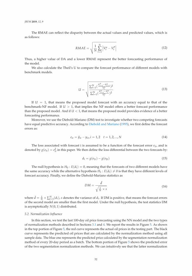
JRFM 2019, 12, 9
The RMAE can reflect the disparity between the actual values and predicted values, which isas follows:
RMAE =
√√√√ 1N
N
∑t=1
∣∣∣Vat − Vp
t
∣∣∣ (12)
Thus, a higher value of DA and a lower RMAE represent the better forecasting performance ofthe model.
We also calculate the Theil’s U to compare the forecast performance of different models withbenchmark models.
U =
√√√√√√∑Nt=1(
Vpt+1−Va
t+1Va
t)2
∑Nt=1(
Vat+1−Va
tVa
t)2
(13)
If U = 1, that means the proposed model forecast with an accuracy equal to that of thebenchmark-NF model. If U > 1, that implies the NF model offers a better forecast performancethan the proposed model. And if U < 1, that means the proposed model provides evidence of a betterforecasting performance.
Moreover, we use the Diebold-Mariano (DM) test to investigate whether two competing forecastshave equal predictive accuracy. According to Diebold and Mariano (1995), we first define the forecasterrors as:
eit = yit − yit, i = 1, 2 t = 1, 2, ..., N (14)
The loss associated with forecast i is assumed to be a function of the forecast error eit, and isdenoted by g(eit) = e2
it in this paper. We then define the loss differential between the two forecasts by:
dt = g(e1t)− g(e2t) (15)
The null hypothesis is H0 : E(dt) = 0, meaning that the forecasts of two different models havethe same accuracy while the alternative hypothesis H1 : E(dt) �= 0 is that they have different levels offorecast accuracy. Finally, we define the Diebold-Mariano statistics as
DM =d√
1N × s
(16)
where d = 1N × ∑N
t=1(dt), s denotes the variance of dt. If DM is positive, that means the forecast errorsof the second model are smaller than the first model. Under the null hypothesis, the test statistics DMis asymptotically N(0, 1) distributed.
5.2. Normalization Influence
In this section, we test the last 100-day oil price forecasting using the NN model and the two typesof normalization methods described in Sections 3.1 and 4. We report the results in Figure 5. As shownin the top portion of Figure 5, the red curve represents the actual oil prices in the testing part. The blackcurve represents the predicted oil prices that are calculated by the normalization method using allsample data. The blue one represents the predicted price calculated by the segmentation normalizationmethod of every 20-day period as a batch. The bottom portion of Figure 5 shows the predicted errorof the two segmentation normalization methods. We can intuitively see that the latter normalization
52
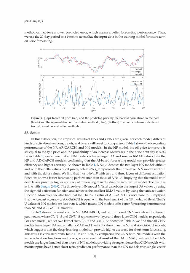
JRFM 2019, 12, 9
method can achieve a lower predicted error, which means a better forecasting performance. Thus,we use the 20-day period as a batch to normalize the input data in the training model for short-termoil price forecasting.
0 10 20 30 40 50 60 70 80 90 10040
45
50
55
OIL
PR
ICE
Norm allTargetNorm 20
0 10 20 30 40 50 60 70 80 90 100
DAY
0
1
2
3
PR
ED
ICT
ED
ER
RO
R
Norm allNorm 20
Figure 5. (Top) Target oil price (red) and the predicted price by the normal normalization method(black) and the segmentation normalization method (blue); (Bottom) The predicted error calculatedfrom different normalization methods.
5.3. Results
In this subsection, the empirical results of NNs and CNNs are given. For each model, differentkinds of activation functions, inputs, and layers will be set for comparison. Table 1 shows the forecastingperformance of the NF, AR-GARCH, and NN models. In the NF model, the oil price tomorrow isset equal to today’s price and the probability of an increase (decrease) in the price next day is 50%.From Table 1, we can see that all NN models achieve larger DA and smaller RMAE values than theNF and AR-GARCH models, confirming that the AI-based forecasting model can provide greaterefficiency and higher accuracy. As shown in Table 1, NNs_A denotes the two-layer NN model withoutand with the delta values of oil prices, while NNs_B represents the three-layer NN model withoutand with the delta values. We find that most NNs_B with two and three layers of different activationfunctions show a better forecasting performance than those of NNs_A, implying that the model withdeep layers provides higher accuracy of forecasting than the shallow architecture model. The result isin line with Bengio (2009). The three-layer NN model NNs_B can obtain the largest DA values by usingthe sigmoid activation function and achieves the smallest RMAE values by using the tanh activationfunction. Moreover, we also find that the Theil’s U value of AR-GARCH is very close to 1, implyingthat the forecast accuracy of AR-GARCH is equal with the benchmark of the NF model, while all Theil’sU values of NN models are less than 1, which means NN models offer better forecasting performancesthan NF and AR-GARCH models.
Table 2 shows the results of the NF, AR-GARCH, and our proposed CNN models with differentparameters, where CNN_A and CNN_B represent two-layer and three-layer CNN models, respectively.For each model, we set two kernel sizes-2 × 2 and 3 × 3. As shown in Table 2, we find that all CNNmodels have larger DA and smaller RMAE and Theil’s U values than the NF and AR-GARCH models,which suggests that the deep-learning model can provide higher accuracy for short-term forecasting.This result is consistent with Table 1. In addition, by comparing the CNN with NN models with thesame activation functions and layers, we can see that most of the DA (RMAE) values of the CNNmodels are larger (smaller) than those of NN models, providing strong evidence that CNN models withmatrix inputs have better short-term prediction performance than the NN models with single-vector
53
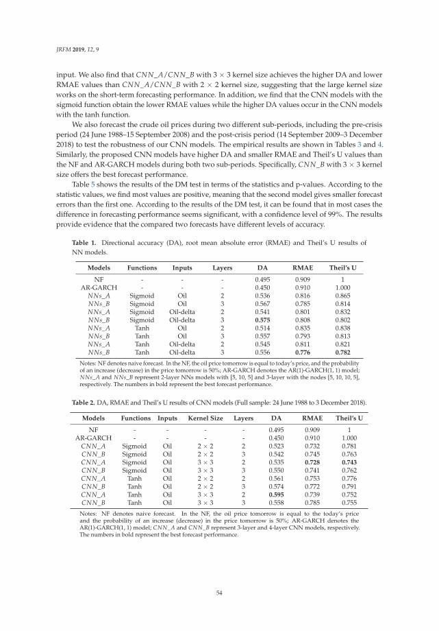
JRFM 2019, 12, 9
input. We also find that CNN_A/CNN_B with 3 × 3 kernel size achieves the higher DA and lowerRMAE values than CNN_A/CNN_B with 2 × 2 kernel size, suggesting that the large kernel sizeworks on the short-term forecasting performance. In addition, we find that the CNN models with thesigmoid function obtain the lower RMAE values while the higher DA values occur in the CNN modelswith the tanh function.
We also forecast the crude oil prices during two different sub-periods, including the pre-crisisperiod (24 June 1988–15 September 2008) and the post-crisis period (14 September 2009–3 December2018) to test the robustness of our CNN models. The empirical results are shown in Tables 3 and 4.Similarly, the proposed CNN models have higher DA and smaller RMAE and Theil’s U values thanthe NF and AR-GARCH models during both two sub-periods. Specifically, CNN_B with 3 × 3 kernelsize offers the best forecast performance.
Table 5 shows the results of the DM test in terms of the statistics and p-values. According to thestatistic values, we find most values are positive, meaning that the second model gives smaller forecasterrors than the first one. According to the results of the DM test, it can be found that in most cases thedifference in forecasting performance seems significant, with a confidence level of 99%. The resultsprovide evidence that the compared two forecasts have different levels of accuracy.
Table 1. Directional accuracy (DA), root mean absolute error (RMAE) and Theil’s U results ofNN models.
Models Functions Inputs Layers DA RMAE Theil’s U
NF - - - 0.495 0.909 1AR-GARCH - - - 0.450 0.910 1.000
NNs_A Sigmoid Oil 2 0.536 0.816 0.865NNs_B Sigmoid Oil 3 0.567 0.785 0.814NNs_A Sigmoid Oil-delta 2 0.541 0.801 0.832NNs_B Sigmoid Oil-delta 3 0.575 0.808 0.802NNs_A Tanh Oil 2 0.514 0.835 0.838NNs_B Tanh Oil 3 0.557 0.793 0.813NNs_A Tanh Oil-delta 2 0.545 0.811 0.821NNs_B Tanh Oil-delta 3 0.556 0.776 0.782
Notes: NF denotes naive forecast. In the NF, the oil price tomorrow is equal to today’s price, and the probabilityof an increase (decrease) in the price tomorrow is 50%; AR-GARCH denotes the AR(1)-GARCH(1, 1) model;NNs_A and NNs_B represent 2-layer NNs models with [5, 10, 5] and 3-layer with the nodes [5, 10, 10, 5],respectively. The numbers in bold represent the best forecast performance.
Table 2. DA, RMAE and Theil’s U results of CNN models (Full sample: 24 June 1988 to 3 December 2018).
Models Functions Inputs Kernel Size Layers DA RMAE Theil’s U
NF - - - - 0.495 0.909 1AR-GARCH - - - - 0.450 0.910 1.000
CNN_A Sigmoid Oil 2 × 2 2 0.523 0.732 0.781CNN_B Sigmoid Oil 2 × 2 3 0.542 0.745 0.763CNN_A Sigmoid Oil 3 × 3 2 0.535 0.728 0.743CNN_B Sigmoid Oil 3 × 3 3 0.550 0.741 0.762CNN_A Tanh Oil 2 × 2 2 0.561 0.753 0.776CNN_B Tanh Oil 2 × 2 3 0.574 0.772 0.791CNN_A Tanh Oil 3 × 3 2 0.595 0.739 0.752CNN_B Tanh Oil 3 × 3 3 0.558 0.785 0.755
Notes: NF denotes naive forecast. In the NF, the oil price tomorrow is equal to the today’s priceand the probability of an increase (decrease) in the price tomorrow is 50%; AR-GARCH denotes theAR(1)-GARCH(1, 1) model; CNN_A and CNN_B represent 3-layer and 4-layer CNN models, respectively.The numbers in bold represent the best forecast performance.
54
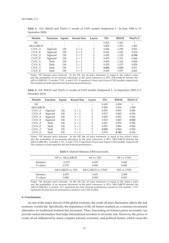
JRFM 2019, 12, 9
Table 3. DA, RMAE and Theil’s U results of CNN models (Subperiod 1: 24 June 1988 to 15September 2008).
Models Functions Inputs Kernel Size Layers DA RMAE Theil’s U
NF - - - - 0.415 1.363 1AR-GARCH - - - - 0.400 1.374 1.001
CNN_A Sigmoid Oil 2 × 2 2 0.436 1.259 0.821CNN_B Sigmoid Oil 2 × 2 3 0.441 1.245 0.814CNN_A Sigmoid Oil 3 × 3 2 0.455 1.129 0.796CNN_B Sigmoid Oil 3 × 3 3 0.475 1.191 0.842CNN_A Tanh Oil 2 × 2 2 0.483 1.162 0.806CNN_B Tanh Oil 2 × 2 3 0.478 1.213 0.829CNN_A Tanh Oil 3 × 3 2 0.492 1.125 0.811CNN_B Tanh Oil 3 × 3 3 0.459 1.257 0.801
Notes: NF denotes naive forecast. In the NF, the oil price tomorrow is equal to the today’s priceand the probability of an increase (decrease) in the price tomorrow is 50%; AR-GARCH denotes theAR(1)-GARCH(1, 1) model; CNN_A and CNN_B represent 3-layer and 4-layer CNN models, respectively.The numbers in bold represent the best forecast performance.
Table 4. DA, RMAE and Theil’s U results of CNN models (Subperiod 2: 14 September 2009 to 3December 2018).
Models Function Inputs Kernel Size Layers DA RMAE Theil’s U
NF - - - - 0.495 0.909 1AR-GARCH - - - - 0.490 0.910 1.000CNN_A Sigmoid Oil 2 × 2 2 0.505 0.891 0.983CNN_B Sigmoid Oil 2 × 2 3 0.517 0.863 0.956CNN_A Sigmoid Oil 3 × 3 2 0.495 0.851 0.942CNN_B Sigmoid Oil 3 × 3 3 0.523 0.865 0.923CNN_A Tanh Oil 2 × 2 2 0.491 0.874 0.996CNN_B Tanh Oil 2 × 2 3 0.501 0.881 0.962CNN_A Tanh Oil 3 × 3 2 0.525 0.884 0.950CNN_B Tanh Oil 3 × 3 3 0.519 0.785 0.956
Notes: NF denotes naive forecast. In the NF, the oil price tomorrow is equal to the today’s priceand the probability of an increase (decrease) in the price tomorrow is 50%; AR-GARCH denotes theAR(1)-GARCH(1, 1) model; CNN_A and CNN_B represent 3-layer and 4-layer CNN models, respectively.The numbers in bold represent the best forecast performance.
Table 5. Diebold-Mariano (DM) test results.
NF vs. AR-GARCH NF vs. NN NF vs. CNN
Statistics −0.313 4.039 3.640P-values 0.755 0.000 0.000
AR-GARCH vs. NN AR-GARCH vs. CNN NN vs. CNN
Statistics 4.035 3.635 2.308P-values 0.000 0.000 0.023
Notes: NF denotes naive forecast. In the NF, the oil price tomorrow is equal to the today’s priceand the probability of an increase (decrease) in the price tomorrow is 50%; AR-GARCH denotes theAR(1)-GARCH(1, 1) model; NN represents the best forecast performance model in NN models; CNNrepresents the best forecast performance model in our CNN models.
6. Conclusions
As one of the major drivers of the global economy, the crude oil price fluctuation affects the realeconomy worldwide. Specifically, the importance of the oil futures markets as a common investmentalternative to traditional markets has increased. Thus, forecasting oil futures prices accurately canprovide useful information that helps international investors to diversify risk. However, the prices ofcrude oil are influenced by many complex natural, economic, and political factors, which cause the
55

JRFM 2019, 12, 9
crude oil futures prices show very complex nonlinear characteristics. Thus, it is very hard to predictthe prices of crude oil accurately by using the traditional economic models. The evolution of a goodforecasting model for oil prices is of great importance.
In this study, we develop a new forecasting methodology based on CNNs to forecast the short-termcrude oil futures prices. We first compare the AI-based deep-learning model with the benchmarkmodels. We then employ the CNN model with matrix inputs for short-term prediction. In our paper,we confirm that the non-linear AI-based deep-learning approach can provide higher accuracy thanthe benchmark models. We also find that the CNNs are more powerful than the benchmark models.These results imply that increasing the dependence of inputs and providing more useful informationare effective ways of improving the forecasting performance.
Author Contributions: Conceptualization: S.H. and T.T.; Formal Analysis: Z.L. and X.C.; Writing—Originaldraft preparation: Z.L. and X.C.; Writing—Reviewing and editing: K.T., T.T., T.K. and S.H.; Funding Acquisition:T.T. and S.H.
Funding: This work was supported by JSPS KAKENHI Grant Number 17K18564 and (A) 17H00983.
Acknowledgments: We would like to acknowledge the valuable comments from the Reviewers of Journal of Riskand Financial Management.
Conflicts of Interest: The authors declare no conflicts of interest.
References
Alvarez-Ramirez, Jose, Eduardo Rodriguez, Esteban Martina, and Carlos Ibarra-Valdez. 2012. Cyclical behaviorof crude oil markets and economic recessions in the period 1986–2010. Technological Forecasting and SocialChange 79: 47–58. [CrossRef]
Baumeister, Christiane, Pierre Guérin, and Lutz Kilian. 2015. Do high-frequency financial data help forecast oilprices? The MIDAS touch at work. International Journal of Forecasting 31: 238–52. [CrossRef]
Bengio, Yoshua. 2009. Learning deep architectures for AI. Foundations and Trends R© in Machine Learning 2: 1–127.[CrossRef]
De Souza e Silva, Edmundo G., Luiz F.L. Legey, and Edmundo A. de Souza e Silva. 2010. Forecasting oil pricetrends using wavelets and hidden Markov models. Energy Economics 32: 1507–19. [CrossRef]
Diebold, Francis X., and Roberto S. Mariano. 1995. Comparing predictive accuracy. Journal of Business andEconomic Statistics 13: 253–63.
Drachal, Krzysztof. 2016. Forecasting spot oil price in a dynamic model averaging framework—Have thedeterminants changed over time? Energy Economics 60: 35–46. [CrossRef]
Jammazi, Rania, and Chaker Aloui. 2012. Crude oil price forecasting: Experimental evidence from waveletdecomposition and neural network modeling. Energy Economics 34: 828–41. [CrossRef]
Kingma, Diederik P., and Jimmy Ba. 2014. Adam: A method for stochastic optimization. arXiv, arXiv:1412.6980.Krizhevsky, Alex, Ilya Sutskever, and Geoffrey E. Hinton. 2012. Imagenet classification with deep convolutional
neural networks. Paper presented at the 25th International Conference on Neural Information ProcessingSystems, Lake Tahoe, NV, USA, December 3–6, pp. 1097–105.
LeCun, Yann, Bernhard E. Boser, John Denker, Don Henderson, Richard E. Howard, Wayne Hubbard, and LarryJackel. 1989. Backpropagation applied to handwritten zip code recognition. Neural Computation 1: 541–51.[CrossRef]
Ma, Xiaolei, Zhuang Dai, Zhengbing He, Jihui Na, Yong Wang, and Yunpeng Wang. 2017. Learning trafficas images: A deep convolutional neural network for large-scale transportation network speed prediction.Sensors 17: 818. [CrossRef] [PubMed]
Merino, Antonio, and Álvaro Ortiz. 2005. Explaining the so-called “price premium” in oil markets. OPEC EnergyReview 29: 133–52. [CrossRef]
Moshiri, Source, and Faezeh Foroutan. 2006. Forecasting nonlinear crude oil futures prices. The Energy Journal 27:81–95. [CrossRef]
Naser, Hanan. 2016. Estimating and forecasting the real prices of crude oil: A data rich model using a dynamicmodel averaging (DMA) approach. Energy Economics 56: 75–87. [CrossRef]
56

JRFM 2019, 12, 9
Ongkrutaraksa, Worapot. 1995. Fractal Theory and Neural Networks in Capital Markets. Working Paper at Kent StateUniversity. Kent: Kent State University.
Refenes, Apostolos Paul. 1994. Neural Networks in the Capital Markets. New York: John Wiley & Sons, Inc.Simonyan, Karen, and Andrew Zisserman. 2014. Two-stream convolutional networks for action recognition in
videos. In Advances in Neural Information Processing Systems. Cambridge: MIT Press, pp. 568–76.Sklibosios Nikitopoulos, Christina, Matthew Squires, Susan Thorp, and Danny Yeung. 2017. Determinants of
the crude oil futures curve: Inventory, consumption and volatility. Journal of Banking and Finance 84: 53–67.[CrossRef]
Tang, Mingming, and Jinliang Zhang. 2012. A multiple adaptive wavelet recurrent neural network model toanalyze crude oil prices. Journal of Economics and Business 64: 275–86.
Wang, Shouyang, Lean Yu, and Kin Keung Lai. 2005. Crude oil price forecasting with TEI@ I methodology.Journal of Systems Science and Complexity 18: 145–66.
Wang, Yudong, Chongfeng Wu, and Li Yang. 2016. Forecasting crude oil market volatility: A Markov switchingmultifractal volatility approach. International Journal of Forecasting 32: 1–9. [CrossRef]
Wen, Fenghua, Xu Gong, and Shenghua Cai. 2016. Forecasting the volatility of crude oil futures using HAR-typemodels with structural breaks. Energy Economics 59: 400–13. [CrossRef]
Yu, Lean, Yang Zhao, and Ling Tang. 2017. Ensemble forecasting for complex time series using sparserepresentation and neural networks. Journal of Forecasting 36: 122–38. [CrossRef]
Ye, Michael, John Zyren, and Joanne Shore. 2006. Forecasting short-run crude oil price using high-andlow-inventory variables. Energy Policy 34: 2736–43. [CrossRef]
Zeiler, Matthew D., and Rob Fergus. 2014. Visualizing and understanding convolutional networks. Paperpresented at the European Conference on Computer Vision, Zurich, Switzerland, September 6–12, pp. 818–33.
Zhao, Yang, Jianping Li, and Lean Yu. 2017. A deep learning ensemble approach for crude oil price forecasting.Energy Economics 66: 9–16. [CrossRef]
c© 2019 by the authors. Licensee MDPI, Basel, Switzerland. This article is an open accessarticle distributed under the terms and conditions of the Creative Commons Attribution(CC BY) license (http://creativecommons.org/licenses/by/4.0/).
57
Journal of
Risk and FinancialManagement
Article
Take Profit and Stop Loss Trading StrategiesComparison in Combination with an MACDTrading System
Dimitrios Vezeris 1,* , Themistoklis Kyrgos 2 and Christos Schinas 1
1 Department of Electrical and Computer Engineering, Democritus University of Thrace,67100 Xanthi, Greece; [email protected]
2 COSMOS4U, 67100 Xanthi, Greece; [email protected]* Correspondence: [email protected]; Tel.: +30-254-108-4084
Received: 22 August 2018; Accepted: 17 September 2018; Published: 19 September 2018
Abstract: A lot of strategies for Take Profit and Stop Loss functionalities have been propoundedand scrutinized over the years. In this paper, we examine various strategies added to a simpleMACD automated trading system and used on selected assets from Forex, Metals, Energy, andCryptocurrencies categories and afterwards, we compare and contrast their results. We concludethat Take Profit strategies based on faster take profit signals on MACD are not better than a simpleMACD strategy and of the different Stop Loss strategies based on ATR, the sliding and variable ATRwindow has the best results for a period of 12 and a multiplier of 6. For the first time, to the bestof our knowledge, we implement a combination of an adaptive MACD Expert Advisor that usesback-tested optimized parameters per asset with price levels defined by the ATR indicator, used toset limits for Stop Loss.
Keywords: algorithmic trading; take profit; stop loss; MACD; ATR
1. Introduction
When trading on an asset, investors are exposed to a potentially high risk if the price movestowards a direction which is the opposite from the one they had anticipated. This could result inconsiderable losses in the investment capital, unless immediate action is taken to exit the non-profitableposition as soon as possible. On the other hand, if the price moves towards a direction that makes thecurrent position profitable, an investor might want to close the position and cash in the profits gainedso far, as there is always the possibility that winning trades could turn into losing positions and lead tocatastrophic losses.
Different strategies of securing profits (Take Profit) and averting losses (Stop Loss) have beenproposed and examined, usually involving the prices at which a position was opened, and arefrequently used by traders, as well as automated trading systems. In this research, we tested andcompared six different Take Profit and Stop Loss strategies used in combination with an algorithmictrading system, based on the MACD indicator on eleven different assets over a six-month period.With the results of these comparisons, we aim to provide some practical insights into every day tradersabout which Take Profit and Stop Loss technics to incorporate with an existing MACD strategy andwhich to avoid. There have been numerous studies about MACD, which is a 30-year-old tool, such asthose by Chong and Ng (2008) and Yazdi and Lashkari (2013), focused on MACD’s performance invarious markets and timeframes, or such as that by Ni and Yin (2009), who examined, among others,Take Profit and Stop Loss technics in MACD using neural networks. But there has not yet been a studyof MACD combined with the Take Profit/Stop Loss strategies we examined based on ATR and in afaster timeframe.
JRFM 2018, 11, 56; doi:10.3390/jrfm11030056 www.mdpi.com/journal/jrfm58

JRFM 2018, 11, 56
2. Materials and Methods
2.1. Trading Systems
2.1.1. Automated Trading
Nowadays, trading is almost exclusively conducted electronically through a computer (Jain 2005).In addition to that, investors have replaced the broker with a platform of automated trading(algorithmic trading), as was postulated by Hendershott and Moulton (2007).
The decrease in the cost of this technology has led to its fast-paced adoption by the financialindustry. The resulting technological change has brought about a revolution in the financial marketsand the way the assets are traded. Many institutions today trade through algorithms and algorithmictrades improve liquidity. It has been proven that the increased algorithmic trades limit wrong pricechoices and decrease the proportion of offer risk over different price levels of an asset associated withthe trades. These results show that algorithmic trading lowers the cost of trades and enhances theinformativeness of quotes, as demonstrated by Hendershott et al. (2011).
On the other hand, it seems that Forex manual trading outweighs automated trading systems.Humans are more informed than systems (Chaboud et al. 2014). However, on closer inspection, werealize that there are some indications pointing to the fact that algorithmic trading contributes to anefficient price discovering process (Brogaard et al. 2014) through the elimination of opportunities fortriangular arbitrage and faster “integration” of macroeconomic news into the price (Foucault et al. 2011).Also, in the same paper, it was established that algorithmic trades tend to correlate, demonstratingthat automated strategies are not that different from those used by a human. Despite that correlation,there are no indications that algorithmic trading causes excess variability. In addition, the volume ofalgorithmic trading in the market has a small, but positive, impact on the liquidity of the market.
In this research, only algorithmic trades are executed without human intervention, with anautomated high frequency trading system. Consequently, commissions and the cost of position swapare kept to a minimum, in contrast with using human intermediaries, and are subsequently presented.But the main element is the fact that they are automatically included in the results by the tradingterminal we used. Consequently, the profit rate presented in this paper is pure, after the deductionof commissions.
2.1.2. Private Investors
As more brokers adopt electronic trading platforms, more private investors opt for automatedalgorithmic trading. It is estimated that private investors lose 2% in the USA market and 3.8% in Taiwanannually (Barber et al. 2008). It has also been calculated that institutional profits are enhanced by 1.5%annually as a result of the small transactions’ cost and corresponding profits of the same actions.
The feeling of the individual investors in relation to weekly and monthly profits and the variabilityof NYSE stocks was studied by Kaniel et al. (2004). Private investors who are more aware of therisk may force them to provide liquidity to other market participants who seek an instant service.The buying orders from bigger, stock-accumulating investors can cause a coercion of sales by increasingthe prices. In the same way, individual buyers are attracted to lower prices caused when these largerinvestors choose to sell their stocks. Liquidity is actually provided by both professional traders(e.g., specialists) and individuals. If we assume that market liquidity is only provided by individualinvestors and they are more active in relation to the demand for immediacy, then there would be anexcess supply of liquidity. In this case, individual investors that have contracts and are silent liquidityproviders will amount losses, while more terms-informed investors will perform trades in adverseconditions. If, on the other hand, there are fewer investors than the market immediacy demands,the silent liquidity providers will amount profits. Understanding the predictability of the short-termprofits calls for an understanding of the silent liquidity provision to individuals, as well as the explicit
59

JRFM 2018, 11, 56
liquidity provision to professional investors. Specifically, the provision of liquidity can be regarded asthe interaction between different types of investors that trade on the same market.
A lot of individuals, in parallel with these systems, adopt long-term positions, instead ofstrategic buying and holding, strategies whose trends are reflected on Google Trends, an analysisby Preis et al. (2013) quantifying the behavior of the market. In this research, there is no liquidityproblem, especially for the $10,000 of initial capital, as the automated systems tested in this research canbe implemented by institutes, as well as by private investors. On the other hand, it has been proventhrough back-testing that whether or not data from the profits of an asset or data from Google Trends areused for the same asset, the results are the same. The results have been tested on a non-linear machinelearning system by Challet and Ayed (2014). In the current work, the problem of back-testing periodselection is evident.
2.2. Take Profit & Stop Loss
Returns can be either absolute or relative. As a rule, we avoid absolute numbers because they willhave to be calculated for each asset individually. Leung and Li (2015) proved that the stop loss functionhas to be calculated at every moment because it is related to the price of an asset at every tick sincethat price is within the price range x ∈ (L, b × L), or the investor, if x is the entering price, can simplyset a constant I (proportional to the fluctuation we add), where x−I is the stop loss price. In addition,returns change over seasons and periods, according to the influences an asset undergoes as a resultof outside or inside factors. It is obvious that orders with stop loss and take profit, when activated,oppose the market trend (take profit) or intensify the movement (stop loss), with great influenceeven over the liquidity during a flash crash (Easley et al. 2011). In all these adoptive trading systems,special consideration should be given to the use of these functions, as shown by Austin et al. (2004).In addition, the use of cut-loss orders and take profit orders and the range of these orders reflect therisk-taking desire of the investor (Au et al. 2003).
With regard to absolute numbers, we see a 3% take profit and a 2% stop loss in the work byBolgün et al. (2010) on stocks of the Istanbul Stock Exchange. Constant take profit was used byKrishnan and Menon (2009), defined at 20 pips, in an interesting work that examined the influencethat rate, closing price times, and indicators participating in trading systems (RSI, BB, Stoch, SAR,MACD, ADX, CCI, Williams %R, Mom, A/D) have on profit. Take profit was also set at 20 pipsby Barbosa and Belo (2010). Even in systems that are based on the flow of buy and sell orders andnot on the price itself, as postulated by Bates et al. (2003), stop loss and take profit were used as afunction of returns 0–0.5%, 0.5–1%, etc. Similarly, Azzini and Tettamanzi (2008b) set staggering takeprofit signals on returns of 0.33%, 0.67%, etc., while in another work, Azzini and Tettamanzi (2008a)took three returns as take profit, logarithmically setting the constant at rTP = 0.006, 0.008, or 0.0046.Martinez et al. (2009) conducted experiments that converted the percentage of loss break from 0.1%to 2.0%. A small loss break percentage could impede profitable transactions, while a high one couldcause bigger losses. The system executes more profitable transactions with the stop loss rules and the0.5% percent yielded the best results.
As for the fluctuation range, we consider that take profit and stop loss functions display flexibilityof profitability adjusted on each asset. In this way, with the range (R), stop loss = 0,5R and take profit= 1R were set by Cervelló-Royo et al. (2015). It is obvious that profit>stop loss is the only fair deal.Consequently, we make sure that 1R > 0.5R. Klement (2013) set the stop loss (c) in combination with areentry condition (d), where (c) as the stop loss level is expressed in units of annual standard deviationof the return of an asset. The same applies for (d). Similarly, Chevallier et al. (2012) set a dynamic stoploss and reduced the losses on S&P500, for which the rule is as follows: if the proposed rate of returnagainst the variability reaches a lower limit (n), that is, the number of fluctuation days of the marketthat will activate the stop loss rule, then this is a signal for the selling of the investment.
We prove here that the addition of take profit and stop loss could considerably improve theresults, to the point that they become profitable, in contrast to the claim laid by Clare et al. (2013).
60

JRFM 2018, 11, 56
More specifically, this became more evident after the proof put forward by Han et al. (2016), who, witha stop loss at 10% of the monthly returns of a strategy based on the momentum, achieved a reductionof losses from −49.79% to −11.36%. Likewise, for monthly data from 1950 to 2004 setting stop loss onAmerican long-term bonds investment, Kaminski and Lo (2014), improved the return over the buyingand holding strategy by 50–100 basis points.
Lei and Li (2009) applied a constant price stop loss, as well as trailing stop loss, for stocks ofNYSE and AMEX from 1970 to 2005. They concluded that the stop loss function shields investorsfrom holding a non-profitable position for a long period of time, which could result in big losses ofcapital. On the other hand, they found a distinction between the profits’ enhancement and the riskreduction. The analysis of exchange rates of high frequency by Osler (2005) yields facts that providesupport for the idea that orders of stop loss have an influence on the fall of prices. First of all, thechange in exchange rates is faster when the prices reach levels at which stop loss orders are usuallyplaced. Secondly, the effect of stop loss orders is greater than the effect of the take profit orders, whichalso helps the fast changes in prices by creating an opposite trend. Thirdly, the effect of stop loss ordershas a broader time duration than that of take profit orders.
All of the above stop loss and take profit rules and conditions can be evaluated and sorted withregard to the profitability of the investment through a number of ways, where the aggregate profitwould be the ultimate result, but with an evaluation framework proposed by Chan and Ma (2015).
The take profit and stop loss functions we use and analyze below are dynamic, follow the averagefluctuation and the current price for every tick, and are activated instantaneously.
2.3. Automated Trading Strategy Development and Combinations
For this research, we used an automated trading system (Expert Advisor) based on the MACDindicator. We started with a simple system and progressively added more complex features,implementing Take Profit and Stop Loss functionalities.
2.3.1. The MACD Indicator and Expert Advisor
The MACD (Moving Average Convergence/Divergence) is a well-known indicator created in1979 by Appel (2005). It calculates the difference of two exponential moving averages of differentperiods over a time-series. The moving average with the smaller period is called the fast movingaverage and the moving average with the bigger period is called the slow moving average.
MACD line = EMAp f ast(Timeseries)− EMApslow(Timeseries), p f ast < pslow (1)
Another exponential moving average is calculated on the MACD line, called the Signal line:
Signal line = EMApsignal (MACD line) (2)
When the MACD line is above the Signal line, this is an indication of an upward trend momentumin the time-series and when the MACD line is below the Signal line, this is an indication of a downwardtrend momentum in the time-series.
The default values of the three periods used in the calculations of the MACD indicator are usuallyp f ast = 12, pslow = 26, and psignal = 9 in the daily timeframe. An example of the MACD indicator canbe seen in Figure 1.
61
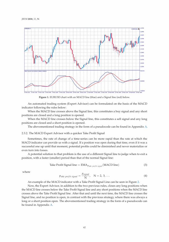
JRFM 2018, 11, 56
Figure 1. EURUSD chart with an MACD line (blue) and a Signal line (red) below.
An automated trading system (Expert Advisor) can be formulated on the basis of the MACDindicator following the rules below:
When the MACD line crosses above the Signal line, this constitutes a buy signal and any shortpositions are closed and a long position is opened.
When the MACD line crosses below the Signal line, this constitutes a sell signal and any longpositions are closed and a short position is opened.
The abovementioned trading strategy in the form of a pseudocode can be found in Appendix A.
2.3.2. The MACD Expert Advisor with a quicker Take Profit Signal
Sometimes, the rate of change of a time-series can be more rapid than the rate at which theMACD indicator can provide us with a signal. If a position was open during that time, even if it was asuccessful one up until that moment, potential profits could be diminished and never materialize oreven turn into losses.
A potential solution to that problem is the use of a different Signal line to judge when to exit aposition, with a faster (smaller) period than that of the normal Signal line:
Take Profit Signal line = EMAptake pro f it signal (MACD line) (3)
whereptake pro f it signal =
psignal
N, N = 2, 3, . . . (4)
An example of the MACD indicator with a Take Profit Signal Line can be seen in Figure 2.Now, the Expert Advisor, in addition to the two previous rules, closes any long positions when
the MACD line crosses below the Take Profit Signal line and any short positions when the MACD linecrosses above the Take Profit Signal line. After that and until the next time, the MACD line crosses theSignal line, and no position is open, in contrast with the previous strategy, where there was always along or a short position open. The abovementioned trading strategy in the form of a pseudocode canbe found in Appendix A.
62
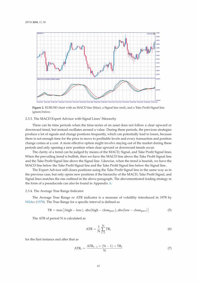
JRFM 2018, 11, 56
Figure 2. EURUSD chart with an MACD line (blue), a Signal line (red), and a Take Profit Signal line(green) below.
2.3.3. The MACD Expert Advisor with Signal Lines’ Hierarchy
There can be time periods when the time-series of an asset does not follow a clear upward ordownward trend, but instead oscillates around a value. During these periods, the previous strategiesproduce a lot of signals and change positions frequently, which can potentially lead to losses, becausethere is not enough time for the price to move to profitable levels and every transaction and positionchange comes at a cost. A more effective option might involve staying out of the market during theseperiods and only opening a new position when clear upward or downward trends occur.
The clarity of a trend can be judged by means of the MACD, Signal, and Take Profit Signal lines.When the prevailing trend is bullish, then we have the MACD line above the Take Profit Signal lineand the Take Profit Signal line above the Signal line. Likewise, when the trend is bearish, we have theMACD line below the Take Profit Signal line and the Take Profit Signal line below the Signal line.
The Expert Advisor still closes positions using the Take Profit Signal line in the same way as inthe previous case, but only opens new positions if the hierarchy of the MACD, Take Profit Signal, andSignal lines matches the one outlined in the above paragraph. The abovementioned trading strategy inthe form of a pseudocode can also be found in Appendix A.
2.3.4. The Average True Range Indicator
The Average True Range or ATR indicator is a measure of volatility introduced in 1978 byWilder (1978). The True Range for a specific interval is defined as
TR = max[(high − low), abs
(high − closeprev
), abs
(low − closeprev
)](5)
The ATR of period N is calculated as
ATR =1N
N
∑i=1
TRi (6)
for the first instance and after that as
ATRt =ATRt−1 × (N − 1) + TRt
N(7)
63
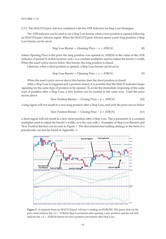
JRFM 2018, 11, 56
2.3.5. The MACD Expert Advisor combined with the ATR Indicator for Stop Loss Strategies
The ATR indicator can be used to set a Stop Loss barrier when a new position is opened followingan MACD Expert Advisor signal. When the MACD Expert Advisor opens a new long position, a StopLoss barrier can be set at
Stop Loss Barrier = Opening Price − x × ATR(N) (8)
where Opening Price is the price the long position was opened at, ATR(N) is the value of the ATRindicator of period N at that moment, and x is a constant multiplier used to adjust the barrier’s width.When the asset’s price moves below that barrier, the long position is closed.
Likewise, when a short position is opened, a Stop Loss barrier can be set at
Stop Loss Barrier = Opening Price + x × ATR(N) (9)
When the asset’s price moves above this barrier, then the short position is closed.After a Stop Loss is triggered and a position closed, it is possible that the MACD indicator keeps
signaling for the same type of position to be opened. To avoid the immediate reopening of the sametype of position after a Stop Loss, a new barrier can be created in the same way. Until the pricemoves above
New Position Barrier = Closing Price + y × ATR(N) (10)
a long signal will not result in a new long position after a Stop Loss, and until the price moves below
New Position Barrier = Closing Price − y × ATR(N) (11)
a short signal will not result in a new short position after a Stop Loss. The y parameter is a constantmultiplier used to adjust the barrier’s width, as is the case with x. Examples of Stop Loss Barriers andNew Position Barriers can be seen in Figure 3. The abovementioned trading strategy in the form of apseudocode can also be found in Appendix A.
Figure 3. A segment from an MACD Expert Advisor’s trading on EURUSD. The green dots on theprice chart indicate the ±2 × ATR(24) Stop Loss barrier after opening a new position and the red dotsindicate the ±2 × ATR(24) barrier for new positions prevention after Stop Loss.
64

JRFM 2018, 11, 56
2.3.6. The MACD Expert Advisor with sliding ATR barrier zone
The ATR Stop Loss barriers described in the above section are drawn around the price at whicha new position is opened and stay fixed, even if the price follows an upward, profitable trend, untilthere is a new MACD signal or the price moves back to the barrier.
In the second case, when the price moves back to the Stop Loss barrier, the potential gains fromthe previous profitable movements are never materialized. To prevent this, the ±x × ATR(N) zone canbe redrawn each time the price moves out of it and follows a profitable direction. This slides the StopLoss barrier to values that secure some of the profits gained so far.
On the other hand, the position prevention barrier should stay at the same level and not slide,as it could prevent the Expert Advisor from opening a new position for a long time. An example ofthis strategy can be seen in Figure 4.
Figure 4. A segment from an MACD Expert Advisor’s trading on EURUSD. The green dots show howthe ±2 × ATR(24) zone slides upwards as the price moves to more profitable values. Eventually, a stoploss is triggered and the position is closed at a higher price than the one we would have in the event ofwaiting for the next MACD signal.
2.3.7. The MACD Expert Advisor with sliding and variable ATR barrier zone
An asset’s price can show large or small variability as it changes over time, which reflects thevalue of ATR. In the previous cases, ATR barriers were of a constant range, calculated with the ATRvalue at the moment when a position opened. Using the latest ATR value to form an ATR window witha variable range through time, could prevent the expert advisor from exiting a position prematurely inperiods when variability spikes and help him follow the price trends, as seen in Figure 5.
65
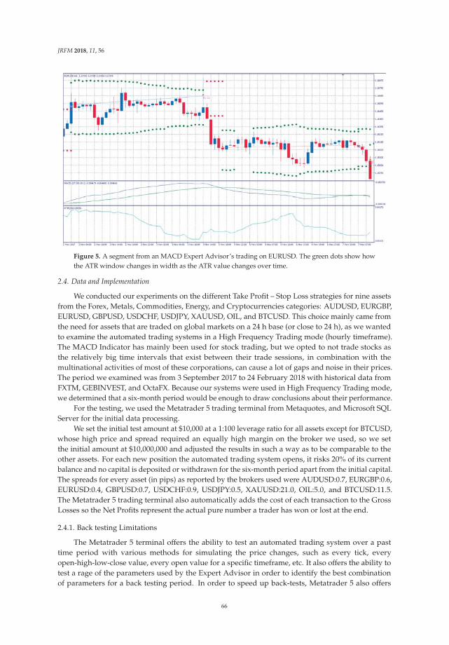
JRFM 2018, 11, 56
Figure 5. A segment from an MACD Expert Advisor’s trading on EURUSD. The green dots show howthe ATR window changes in width as the ATR value changes over time.
2.4. Data and Implementation
We conducted our experiments on the different Take Profit – Stop Loss strategies for nine assetsfrom the Forex, Metals, Commodities, Energy, and Cryptocurrencies categories: AUDUSD, EURGBP,EURUSD, GBPUSD, USDCHF, USDJPY, XAUUSD, OIL, and BTCUSD. This choice mainly came fromthe need for assets that are traded on global markets on a 24 h base (or close to 24 h), as we wantedto examine the automated trading systems in a High Frequency Trading mode (hourly timeframe).The MACD Indicator has mainly been used for stock trading, but we opted to not trade stocks asthe relatively big time intervals that exist between their trade sessions, in combination with themultinational activities of most of these corporations, can cause a lot of gaps and noise in their prices.The period we examined was from 3 September 2017 to 24 February 2018 with historical data fromFXTM, GEBINVEST, and OctaFX. Because our systems were used in High Frequency Trading mode,we determined that a six-month period would be enough to draw conclusions about their performance.
For the testing, we used the Metatrader 5 trading terminal from Metaquotes, and Microsoft SQLServer for the initial data processing.
We set the initial test amount at $10,000 at a 1:100 leverage ratio for all assets except for BTCUSD,whose high price and spread required an equally high margin on the broker we used, so we setthe initial amount at $10,000,000 and adjusted the results in such a way as to be comparable to theother assets. For each new position the automated trading system opens, it risks 20% of its currentbalance and no capital is deposited or withdrawn for the six-month period apart from the initial capital.The spreads for every asset (in pips) as reported by the brokers used were AUDUSD:0.7, EURGBP:0.6,EURUSD:0.4, GBPUSD:0.7, USDCHF:0.9, USDJPY:0.5, XAUUSD:21.0, OIL:5.0, and BTCUSD:11.5.The Metatrader 5 trading terminal also automatically adds the cost of each transaction to the GrossLosses so the Net Profits represent the actual pure number a trader has won or lost at the end.
2.4.1. Back testing Limitations
The Metatrader 5 terminal offers the ability to test an automated trading system over a pasttime period with various methods for simulating the price changes, such as every tick, everyopen-high-low-close value, every open value for a specific timeframe, etc. It also offers the ability totest a rage of the parameters used by the Expert Advisor in order to identify the best combinationof parameters for a back testing period. In order to speed up back-tests, Metatrader 5 also offers
66

JRFM 2018, 11, 56
the ability to use distributed testing agents utilizing the resources of a local network of computers.We used this ability to form a local cluster of computers, mainly with i5, i7, and Xeon Intel CPUs for atotal capacity of 130 distributed agents, in order to run our backtesting experiments. We also used aMicrosoft SQL Server in order to save and process the results of our experiments during the stage ofparameter selection.
It should be noted that the wider the parameters’ ranges, the greater the number of combinations ofparameters. Also, back testing with an every tick simulation is far more time- and resource-consumingthan back testing with open-high-low-close value, which is in turn more time-consuming than an openvalue only simulation.
The values of the MACD and ATR indicators are calculated over one-hour timeframes, but duringan hourly timeframe, the price of an asset can reach levels that would trigger a Take Profit/Stop Lossin some strategies or an automatic Stop Loss from the broker, so we chose to run our experiments withevery tick simulations.
2.4.2. Parameter Selection
For our tests, we had to choose a set of parameters for each asset that would allow for thedemonstration of an improvement or worsening in the MACD Expert Advisor’s behavior with theintroduction of each Take Profit/Stop Loss strategy.
Since the different periods in the MACD averages can generate widely different results and inorder to render the role of these parameters less significant for our tests, we decided to choose sets ofparameters that are centered on neighborhoods (±2) of similar results, with the results indicating thereis room for both improvement and worsening.
The simple MACD Expert Advisor has three parameters, the periods of its moving averages, whichmeans that even for small parameter ranges, the number of combinations is significant. Performing aback test for every asset with full parameter sweeping on an every tick simulation would be prohibitivebecause of the time and electrical energy it would require. We circumvented this firstly by running thesimulations on open-high-low-close prices ticks, which produces results close enough to the real ticksimulation, and secondly by incrementing each parameter by a step of 2 instead of 1, which reducesthe combinations to 1/8, allowing us to check a wider range. Potentially suitable neighborhoods canstill be identified as a step of 2 still hits a ±2 neighborhood in eight or 27 of its 125 members.
Next, we defined some requirements for a suitable neighborhood, such as a minimum amountof trades and profit range, and chose the best 100 neighborhoods that fulfilled them, sorted by thesmallest relative range defined as
Relative Range =max(Profits)− min(Profits)
average(Profits)(12)
The specific requirements for each asset can be seen in Table 1.
Table 1. Requirements set for neighborhood selection for each asset.
Profits ∈ Trades≥ Central Value
AUDUSD [0, 22500] 59EURGBP [−2800, 10800] 75EURUSD [1500, 6500] 75 MinProfit < 4000 < MaxProfitGBPUSD [0, 8500] 75 MinProfit < 4000 < MaxProfitUSDCHF [400, 7600] 75 MinProfit < 4000 < MaxProfitUSDJPY [200, 7800] 75 MinProfit < 4000 < MaxProfit
XAUUSD [0, 1300] 75 MinProfit < 400 < MaxProfitOIL [0, 30000] 70
BTCUSD [0, 220] 75
67
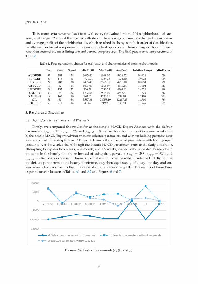
JRFM 2018, 11, 56
To be more certain, we ran back tests with every tick value for these 100 neighborhoods of eachasset, with range ±2 around their center with step 1. The missing combinations changed the min, maxand average profits of the neighborhoods, which resulted in changes in their order of classification.Finally, we conducted a supervisory review of the best options and chose a neighborhood for eachasset that seemed the most fitting one and served our purposes. The final parameters are presented inTable 2.
Table 2. Final parameters chosen for each asset and characteristics of their neighborhoods.
Fast Slow Signal MinProfit MaxProfit AvgProfit Relative Range MinTrades
AUDUSD 57 284 34 3693.40 8969.10 5918.32 0.8914 59EURGBP 27 118 6 −672.23 4324.72 1274.10 3.9220 135EURUSD 27 280 28 2403.46 6166.85 4210.10 0.8939 79GBPUSD 15 82 14 1063.08 8268.69 4648.14 1.5502 129USDCHF 29 132 22 736.39 6780.59 4161.61 1.4524 80USDJPY 33 64 32 1702.63 5914.10 3545.61 1.1878 86
XAUUSD 17 160 16 240.32 1230.11 792.88 1.2484 108OIL 51 60 34 5537.31 21058.19 12217.25 1.2704 76
BTCUSD 53 210 14 48.46 219.93 143.53 1.1946 77
3. Results and Discussion
3.1. Default/Selected Parameters and Weekends
Firstly, we compared the results for a) the simple MACD Expert Advisor with the defaultparameters p f ast = 12, pslow = 26, and psignal = 9 and without holding positions over weekends;b) the simple MACD Expert Advisor with our selected parameters and without holding positions overweekends; and c) the simple MACD Expert Advisor with our selected parameters with holding openpositions over the weekends. Although the default MACD parameters refer to the daily timeframe,attempting to express two weeks, one month, and 1.5 weeks, respectively, we opted to keep themthe same in the hourly timeframe instead of using the equivalent p f ast = 288, pslow = 624, andpsignal = 216 of days expressed in hours since that would move the scale outside the HFT. By portingthe default parameters to the hourly timeframe, they then expressed 1
2 of a day, one day, and onework-day, which is closer to the timeframe of a daily trader doing HFT. The results of these threeexperiments can be seen in Tables A1 and A2 and Figures 6 and 7.
-15000
-10000
-5000
0
5000
10000
AUDUSD EURGBP EURUSD GBPUSD USDCHF USDJPY XAUUSD OIL BTCUSD
a) Default parameters without weekends b) Selected parameters without weekends
c) Selected parameters with weekends
Figure 6. Net Profits of experiments (a), (b), and (c).
68

JRFM 2018, 11, 56
0
10
20
30
40
50
60
70
80
90
100
AUDUSD EURGBP EURUSD GBPUSD USDCHF USDJPY XAUUSD OIL BTCUSD
a) Default parameters without weekends b) Selected parameters without weekends
c) Selected parameters with weekends
Figure 7. Drawdown, as percentage of equity, of experiments (a), (b), and (c).
It can be concluded that holding open positions over the weekends helps cut one’s losses, butit also takes away a proportion of the profits for all the examined assets. Figure 6 makes clear thatthe net profits in most cases are diminished and Figure 7 shows the usually higher drawdown whenholding positions open over the weekend. Also, using the default parameters almost always results inlosses. Because of differences in contract sizes, trading hours, variability, etc., the XAUUSD, OIL, andBTCUSD show different numbers compared with the FOREX pairs (a behavior that also presents itselfto the rest of the experiments) but, in the relativity of the experiments’ comparisons, their numbers stillsupport the conclusions. The Net Profits in Table A1 and, by extension, for all later experiments, are aresult of the parameter selection described in Section 2.4.2., which is a posteriori process. The actualamount of returns and the profitability of the MACD Expert Advisor are not something we actuallyconcern ourselves with in this research, but rather how these returns change by adding each TakeProfit and Stop Loss strategy.
From now on, in our experiments, we will be using our selected parameters for each asset andopen positions will be closed for the weekends.
3.2. Fast Take Profit Signal and Signals’ Hierarchy
Next, we compared the (b) simple MACD Expert Advisor with the (d) MACD Expert Advisor,with the addition of a faster take profit signal, as described in Section 2.3.2. The determined valueof the divisor N of the Fast Signal period was set as follows: N = {2,3,4}. With N = 1, the (d) ExpertAdvisor effectively becomes the same as (b), as the Fast Signal line becomes identical to the Signal line.Their results can be seen in Tables A3 and A4 and Figures 8 and 9.
The simple MACD yields better results in most cases, both in terms of net profits and drawdown,especially on Forex pairs. Even when assets which are traded using the MACD do not yield the mostprofitable results, it is postulated that the MACD ranks second after a neck-and-neck round, with afast Take Profit signal of N = 2.
Next, we compared the (b) simple MACD Expert Advisor with the (e) MACD Expert Advisorthat only opens new positions when the hierarchy of the MACD and Signal lines is right, as describedin Section 2.3.3. The divisor N of the Fast Signal period assumed values of N = {2,3,4}. With N = 1,the e) Expert Advisor becomes the same as (b). Their results can be seen in Tables A5 and A6 andFigures 10 and 11.
69
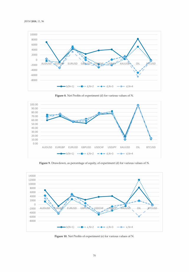
JRFM 2018, 11, 56
-8000
-6000
-4000
-2000
0
2000
4000
6000
8000
10000
AUDUSD EURGBP EURUSD GBPUSD USDCHF USDJPY XAUUSD OIL BTCUSD
b(N=1) d,N=2 d,N=3 d,N=4
Figure 8. Net Profits of experiment (d) for various values of N.
0.0010.0020.0030.0040.0050.0060.0070.0080.0090.00
100.00
AUDUSD EURGBP EURUSD GBPUSD USDCHF USDJPY XAUUSD OIL BTCUSD
b(N=1) d,N=2 d,N=3 d,N=4
Figure 9. Drawdown, as percentage of equity, of experiment (d) for various values of N.
-8000-6000-4000-2000
02000400060008000
100001200014000
AUDUSD EURGBP EURUSD GBPUSD USDCHF USDJPY XAUUSD OIL BTCUSD
b(N=1) e,N=2 e,N=3 e,N=4
Figure 10. Net Profits of experiment (e) for various values of N.
70
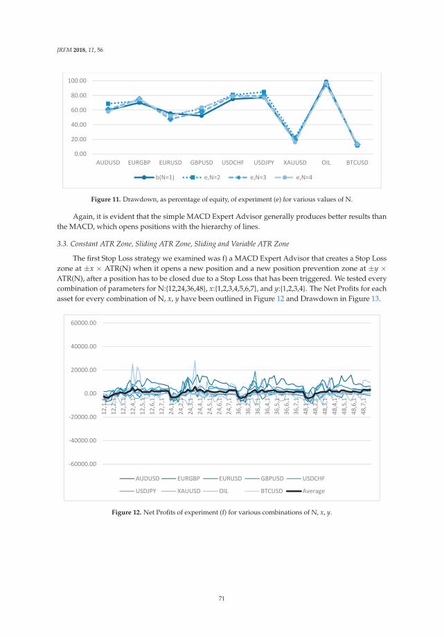
JRFM 2018, 11, 56
0.00
20.00
40.00
60.00
80.00
100.00
AUDUSD EURGBP EURUSD GBPUSD USDCHF USDJPY XAUUSD OIL BTCUSD
b(N=1) e,N=2 e,N=3 e,N=4
Figure 11. Drawdown, as percentage of equity, of experiment (e) for various values of N.
Again, it is evident that the simple MACD Expert Advisor generally produces better results thanthe MACD, which opens positions with the hierarchy of lines.
3.3. Constant ATR Zone, Sliding ATR Zone, Sliding and Variable ATR Zone
The first Stop Loss strategy we examined was f) a MACD Expert Advisor that creates a Stop Losszone at ±x × ATR(N) when it opens a new position and a new position prevention zone at ±y ×ATR(N), after a position has to be closed due to a Stop Loss that has been triggered. We tested everycombination of parameters for N:{12,24,36,48}, x:{1,2,3,4,5,6,7}, and y:{1,2,3,4}. The Net Profits for eachasset for every combination of N, x, y have been outlined in Figure 12 and Drawdown in Figure 13.
-60000.00
-40000.00
-20000.00
0.00
20000.00
40000.00
60000.00
12,1
,112
,2,1
12,3
,112
,4,1
12,5
,112
,6,1
12,7
,124
,1,1
24,2
,124
,3,1
24,4
,124
,5,1
24,6
,124
,7,1
36,1
,136
,2,1
36,3
,136
,4,1
36,5
,136
,6,1
36,7
,148
,1,1
48,2
,148
,3,1
48,4
,148
,5,1
48,6
,148
,7,1
AUDUSD EURGBP EURUSD GBPUSD USDCHF
USDJPY XAUUSD OIL BTCUSD Average
Figure 12. Net Profits of experiment (f) for various combinations of N, x, y.
71
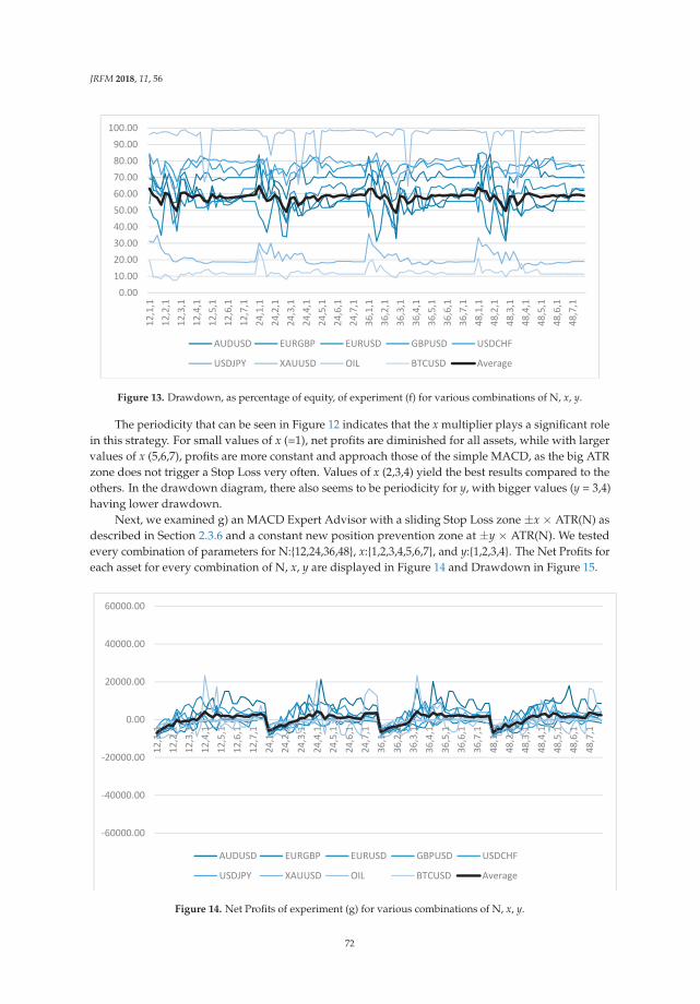
JRFM 2018, 11, 56
0.0010.0020.0030.0040.0050.0060.0070.0080.0090.00
100.00
12,1
,112
,2,1
12,3
,112
,4,1
12,5
,112
,6,1
12,7
,124
,1,1
24,2
,124
,3,1
24,4
,124
,5,1
24,6
,124
,7,1
36,1
,136
,2,1
36,3
,136
,4,1
36,5
,136
,6,1
36,7
,148
,1,1
48,2
,148
,3,1
48,4
,148
,5,1
48,6
,148
,7,1
AUDUSD EURGBP EURUSD GBPUSD USDCHF
USDJPY XAUUSD OIL BTCUSD Average
Figure 13. Drawdown, as percentage of equity, of experiment (f) for various combinations of N, x, y.
The periodicity that can be seen in Figure 12 indicates that the x multiplier plays a significant rolein this strategy. For small values of x (=1), net profits are diminished for all assets, while with largervalues of x (5,6,7), profits are more constant and approach those of the simple MACD, as the big ATRzone does not trigger a Stop Loss very often. Values of x (2,3,4) yield the best results compared to theothers. In the drawdown diagram, there also seems to be periodicity for y, with bigger values (y = 3,4)having lower drawdown.
Next, we examined g) an MACD Expert Advisor with a sliding Stop Loss zone ±x × ATR(N) asdescribed in Section 2.3.6 and a constant new position prevention zone at ±y × ATR(N). We testedevery combination of parameters for N:{12,24,36,48}, x:{1,2,3,4,5,6,7}, and y:{1,2,3,4}. The Net Profits foreach asset for every combination of N, x, y are displayed in Figure 14 and Drawdown in Figure 15.
-60000.00
-40000.00
-20000.00
0.00
20000.00
40000.00
60000.00
12,1
,112
,2,1
12,3
,112
,4,1
12,5
,112
,6,1
12,7
,124
,1,1
24,2
,124
,3,1
24,4
,124
,5,1
24,6
,124
,7,1
36,1
,136
,2,1
36,3
,136
,4,1
36,5
,136
,6,1
36,7
,148
,1,1
48,2
,148
,3,1
48,4
,148
,5,1
48,6
,148
,7,1
AUDUSD EURGBP EURUSD GBPUSD USDCHF
USDJPY XAUUSD OIL BTCUSD Average
Figure 14. Net Profits of experiment (g) for various combinations of N, x, y.
72
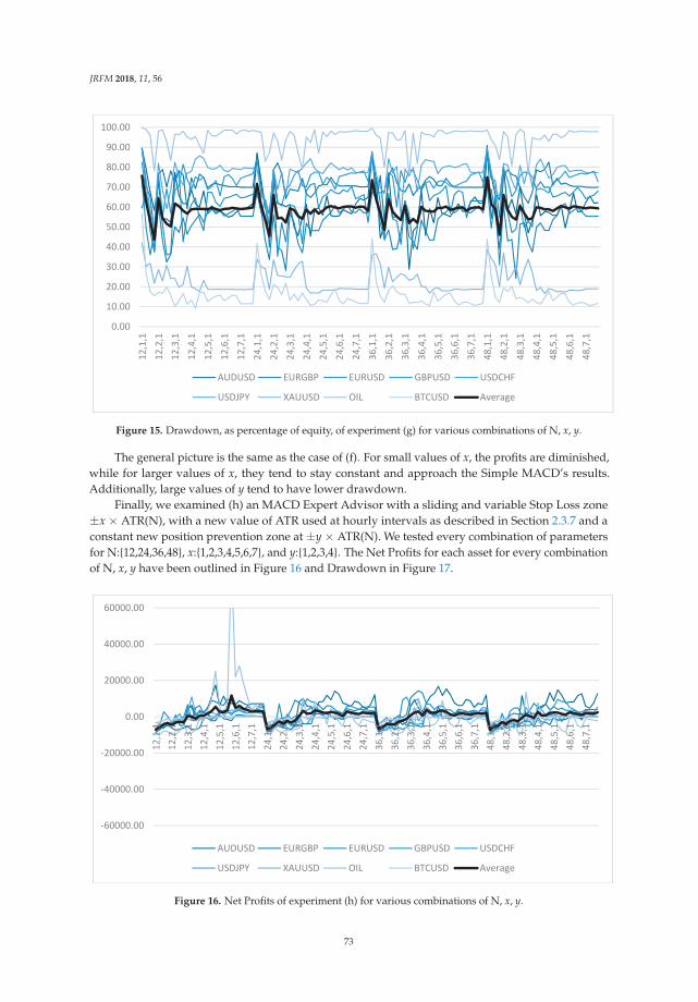
JRFM 2018, 11, 56
0.00
10.00
20.00
30.00
40.00
50.00
60.00
70.00
80.00
90.00
100.0012
,1,1
12,2
,112
,3,1
12,4
,112
,5,1
12,6
,112
,7,1
24,1
,124
,2,1
24,3
,124
,4,1
24,5
,124
,6,1
24,7
,136
,1,1
36,2
,136
,3,1
36,4
,136
,5,1
36,6
,136
,7,1
48,1
,148
,2,1
48,3
,148
,4,1
48,5
,148
,6,1
48,7
,1
AUDUSD EURGBP EURUSD GBPUSD USDCHF
USDJPY XAUUSD OIL BTCUSD Average
Figure 15. Drawdown, as percentage of equity, of experiment (g) for various combinations of N, x, y.
The general picture is the same as the case of (f). For small values of x, the profits are diminished,while for larger values of x, they tend to stay constant and approach the Simple MACD’s results.Additionally, large values of y tend to have lower drawdown.
Finally, we examined (h) an MACD Expert Advisor with a sliding and variable Stop Loss zone±x × ATR(N), with a new value of ATR used at hourly intervals as described in Section 2.3.7 and aconstant new position prevention zone at ±y × ATR(N). We tested every combination of parametersfor N:{12,24,36,48}, x:{1,2,3,4,5,6,7}, and y:{1,2,3,4}. The Net Profits for each asset for every combinationof N, x, y have been outlined in Figure 16 and Drawdown in Figure 17.
-60000.00
-40000.00
-20000.00
0.00
20000.00
40000.00
60000.00
12,1
,112
,2,1
12,3
,112
,4,1
12,5
,112
,6,1
12,7
,124
,1,1
24,2
,124
,3,1
24,4
,124
,5,1
24,6
,124
,7,1
36,1
,136
,2,1
36,3
,136
,4,1
36,5
,136
,6,1
36,7
,148
,1,1
48,2
,148
,3,1
48,4
,148
,5,1
48,6
,148
,7,1
AUDUSD EURGBP EURUSD GBPUSD USDCHF
USDJPY XAUUSD OIL BTCUSD Average
Figure 16. Net Profits of experiment (h) for various combinations of N, x, y.
73
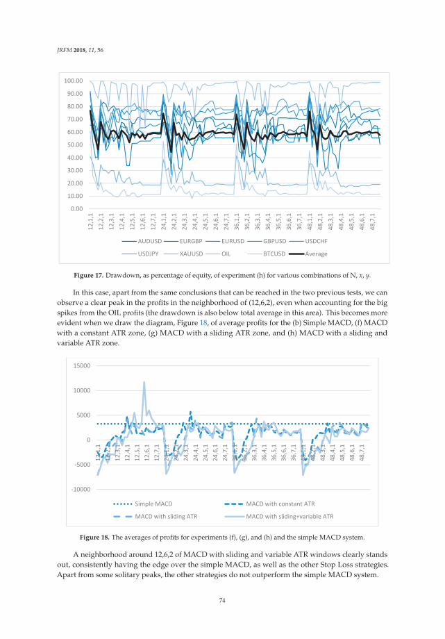
JRFM 2018, 11, 56
0.00
10.00
20.00
30.00
40.00
50.00
60.00
70.00
80.00
90.00
100.0012
,1,1
12,2
,112
,3,1
12,4
,112
,5,1
12,6
,112
,7,1
24,1
,124
,2,1
24,3
,124
,4,1
24,5
,124
,6,1
24,7
,136
,1,1
36,2
,136
,3,1
36,4
,136
,5,1
36,6
,136
,7,1
48,1
,148
,2,1
48,3
,148
,4,1
48,5
,148
,6,1
48,7
,1
AUDUSD EURGBP EURUSD GBPUSD USDCHF
USDJPY XAUUSD OIL BTCUSD Average
Figure 17. Drawdown, as percentage of equity, of experiment (h) for various combinations of N, x, y.
In this case, apart from the same conclusions that can be reached in the two previous tests, we canobserve a clear peak in the profits in the neighborhood of (12,6,2), even when accounting for the bigspikes from the OIL profits (the drawdown is also below total average in this area). This becomes moreevident when we draw the diagram, Figure 18, of average profits for the (b) Simple MACD, (f) MACDwith a constant ATR zone, (g) MACD with a sliding ATR zone, and (h) MACD with a sliding andvariable ATR zone.
-10000
-5000
0
5000
10000
15000
12,1
,112
,2,1
12,3
,112
,4,1
12,5
,112
,6,1
12,7
,124
,1,1
24,2
,124
,3,1
24,4
,124
,5,1
24,6
,124
,7,1
36,1
,136
,2,1
36,3
,136
,4,1
36,5
,136
,6,1
36,7
,148
,1,1
48,2
,148
,3,1
48,4
,148
,5,1
48,6
,148
,7,1
Simple MACD MACD with constant ATR
MACD with sliding ATR MACD with sliding+variable ATR
Figure 18. The averages of profits for experiments (f), (g), and (h) and the simple MACD system.
A neighborhood around 12,6,2 of MACD with sliding and variable ATR windows clearly standsout, consistently having the edge over the simple MACD, as well as the other Stop Loss strategies.Apart from some solitary peaks, the other strategies do not outperform the simple MACD system.
74

JRFM 2018, 11, 56
4. Conclusions
In the present research, we examined various Take Profit and Stop Loss strategies added to asimple MACD automated trading system used in trading 10 assets from the Forex, Metals, Energy, andCryptocurrencies categories. In order to make the MACD parameters less important in our research,we chose parameters based on the characteristics of their neighborhoods of ±2 and used them for allour experiments.
In our research, we first of all concluded that it is generally less profitable to keep positions openduring weekends. Another conclusion we reached is that Take Profit strategies based on faster takeprofit signals on MACD are not far better than a simple MACD strategy. We also showed that amongthe different Stop Loss strategies based on ATR windows, the best and safest results come from asliding and variable ±x × ATR(N) window with period N = 12 and multiplier x = 6 after opening aposition and a constant ±y × ATR(N) with period N = 12 and multiplier y = 2 after stop loss closing.
Since the MACD Indicator is used quite prevalently by a lot of traders and our results are generalenough, a trader could incorporate them in their technical analysis/trading strategy for Stop Loss andTake Profit without interfering with the rest of their strategy (portfolio management, capital allocation,MACD parameter selection, etc.)
Author Contributions: Conceptualization, D.V.; Investigation, D.V.; Methodology, D.V.; Software, T.K.; Supervision,C.S.; Visualization, T.K.
Funding: This research has been co-financed by the European Union and Greek national funds throughthe Operational Program Competitiveness, Entrepreneurship and Innovation, under the call RESEARCH—CREATE—INNOVATE (project code:T1EDK-02342).
Acknowledgments: We would like to thank COSMOS4U for providing the infrastructure used to conduct thisresearch. We would also like to thank the anonymous referees who reviewed our paper and provided us withvaluable insights and suggestions.
Conflicts of Interest: The authors declare no conflict of interest. The funders had no role in the design of thestudy; in the collection, analyses, or interpretation of data; in the writing of the manuscript, and in the decision topublish the results.
Appendix A
Pseudocode of the basic MACD trading strategy as described in Section 2.3.1.
OnTick()
{
if(MACD line > Signal line)
{
if(ShortPositionsExist) CloseShortPositions();
if(!LongPositionsExist) OpenLongPosition();
}
else if(MACD line < Signal line)
{
if(LongPositionsExist) CloseLongPositions();
if(!ShortPositionsExist) OpenShortPosition();
}
}
75

JRFM 2018, 11, 56
Pseudocode of the MACD trading strategy with a faster Take Profit Signal, as described inSection 2.3.2.
OnTick()
{
if(MACD line > Take Profit Signal line)
CloseShortPositions();
else if(MACD line < Take Profit Signal line)
CloseLongPositions();
if( (MACD line > Signal line) && (MACD line > Take Profit Signal line) )
{
if(ShortPositionsExist) CloseShortPositions();
if(!LongPositionsExist) OpenLongPosition();
}
else if( (MACD line < Signal line) && (MACD line < Take Profit Signal line) )
{
if(LongPositionsExist) CloseLongPositions();
if(!ShortPositionsExist) OpenShortPosition();
}
}
Pseudocode of the MACD trading strategy using the Signal Lines’ Hierarchy, as described inSection 2.3.3.
OnTick()
{
if(MACD line > Take Profit Signal line)
CloseShortPositions();
else if(MACD line < Take Profit Signal line)
CloseLongPositions();
if( MACD line > Take Profit Signal line > Signal line )
{
if(ShortPositionsExist) CloseShortPositions();
if(!LongPositionsExist) OpenLongPosition();
}
else if( MACD line < Take Profit Signal line < Signal line )
{
if(LongPositionsExist) CloseLongPositions();
if(!ShortPositionsExist) OpenShortPosition();
}
}
76
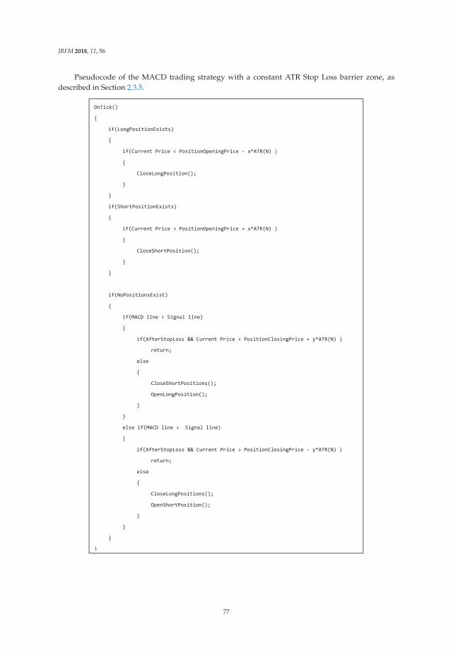
JRFM 2018, 11, 56
Pseudocode of the MACD trading strategy with a constant ATR Stop Loss barrier zone, asdescribed in Section 2.3.5.
OnTick()
{
if(LongPositionExists)
{
if(Current Price < PositionOpeningPrice - x*ATR(N) )
{
CloseLongPosition();
}
}
if(ShortPositionExists)
{
if(Current Price > PositionOpeningPrice + x*ATR(N) )
{
CloseShortPosition();
}
}
if(NoPositionsExist)
{
if(MACD line > Signal line)
{
if(AfterStopLoss && Current Price < PositionClosingPrice + y*ATR(N) )
return;
else
{
CloseShortPositions();
OpenLongPosition();
}
}
else if(MACD line < Signal line)
{
if(AfterStopLoss && Current Price > PositionClosingPrice - y*ATR(N) )
return;
else
{
CloseLongPositions();
OpenShortPosition();
}
}
}
}
77
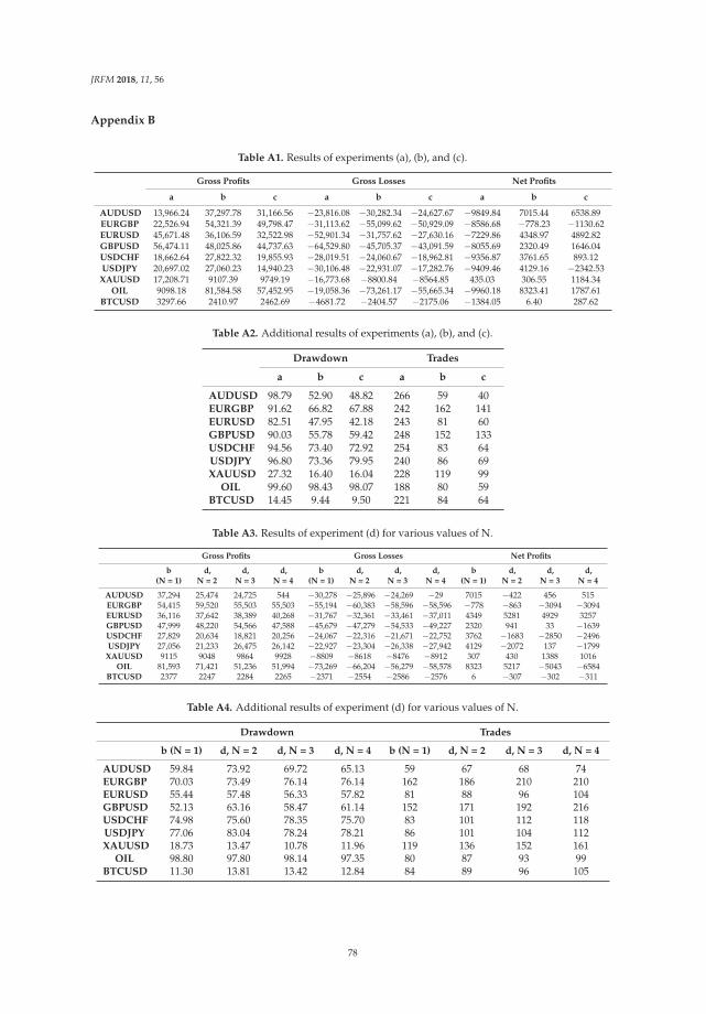
JRFM 2018, 11, 56
Appendix B
Table A1. Results of experiments (a), (b), and (c).
Gross Profits Gross Losses Net Profits
a b c a b c a b c
AUDUSD 13,966.24 37,297.78 31,166.56 −23,816.08 −30,282.34 −24,627.67 −9849.84 7015.44 6538.89EURGBP 22,526.94 54,321.39 49,798.47 −31,113.62 −55,099.62 −50,929.09 −8586.68 −778.23 −1130.62EURUSD 45,671.48 36,106.59 32,522.98 −52,901.34 −31,757.62 −27,630.16 −7229.86 4348.97 4892.82GBPUSD 56,474.11 48,025.86 44,737.63 −64,529.80 −45,705.37 −43,091.59 −8055.69 2320.49 1646.04USDCHF 18,662.64 27,822.32 19,855.93 −28,019.51 −24,060.67 −18,962.81 −9356.87 3761.65 893.12USDJPY 20,697.02 27,060.23 14,940.23 −30,106.48 −22,931.07 −17,282.76 −9409.46 4129.16 −2342.53
XAUUSD 17,208.71 9107.39 9749.19 −16,773.68 −8800.84 −8564.85 435.03 306.55 1184.34OIL 9098.18 81,584.58 57,452.95 −19,058.36 −73,261.17 −55,665.34 −9960.18 8323.41 1787.61
BTCUSD 3297.66 2410.97 2462.69 −4681.72 −2404.57 −2175.06 −1384.05 6.40 287.62
Table A2. Additional results of experiments (a), (b), and (c).
Drawdown Trades
a b c a b c
AUDUSD 98.79 52.90 48.82 266 59 40EURGBP 91.62 66.82 67.88 242 162 141EURUSD 82.51 47.95 42.18 243 81 60GBPUSD 90.03 55.78 59.42 248 152 133USDCHF 94.56 73.40 72.92 254 83 64USDJPY 96.80 73.36 79.95 240 86 69XAUUSD 27.32 16.40 16.04 228 119 99
OIL 99.60 98.43 98.07 188 80 59BTCUSD 14.45 9.44 9.50 221 84 64
Table A3. Results of experiment (d) for various values of N.
Gross Profits Gross Losses Net Profits
b(N = 1)
d,N = 2
d,N = 3
d,N = 4
b(N = 1)
d,N = 2
d,N = 3
d,N = 4
b(N = 1)
d,N = 2
d,N = 3
d,N = 4
AUDUSD 37,294 25,474 24,725 544 −30,278 −25,896 −24,269 −29 7015 −422 456 515EURGBP 54,415 59,520 55,503 55,503 −55,194 −60,383 −58,596 −58,596 −778 −863 −3094 −3094EURUSD 36,116 37,642 38,389 40,268 −31,767 −32,361 −33,461 −37,011 4349 5281 4929 3257GBPUSD 47,999 48,220 54,566 47,588 −45,679 −47,279 −54,533 −49,227 2320 941 33 −1639USDCHF 27,829 20,634 18,821 20,256 −24,067 −22,316 −21,671 −22,752 3762 −1683 −2850 −2496USDJPY 27,056 21,233 26,475 26,142 −22,927 −23,304 −26,338 −27,942 4129 −2072 137 −1799
XAUUSD 9115 9048 9864 9928 −8809 −8618 −8476 −8912 307 430 1388 1016OIL 81,593 71,421 51,236 51,994 −73,269 −66,204 −56,279 −58,578 8323 5217 −5043 −6584
BTCUSD 2377 2247 2284 2265 −2371 −2554 −2586 −2576 6 −307 −302 −311
Table A4. Additional results of experiment (d) for various values of N.
Drawdown Trades
b (N = 1) d, N = 2 d, N = 3 d, N = 4 b (N = 1) d, N = 2 d, N = 3 d, N = 4
AUDUSD 59.84 73.92 69.72 65.13 59 67 68 74EURGBP 70.03 73.49 76.14 76.14 162 186 210 210EURUSD 55.44 57.48 56.33 57.82 81 88 96 104GBPUSD 52.13 63.16 58.47 61.14 152 171 192 216USDCHF 74.98 75.60 78.35 75.70 83 101 112 118USDJPY 77.06 83.04 78.24 78.21 86 101 104 112XAUUSD 18.73 13.47 10.78 11.96 119 136 152 161
OIL 98.80 97.80 98.14 97.35 80 87 93 99BTCUSD 11.30 13.81 13.42 12.84 84 89 96 105
78
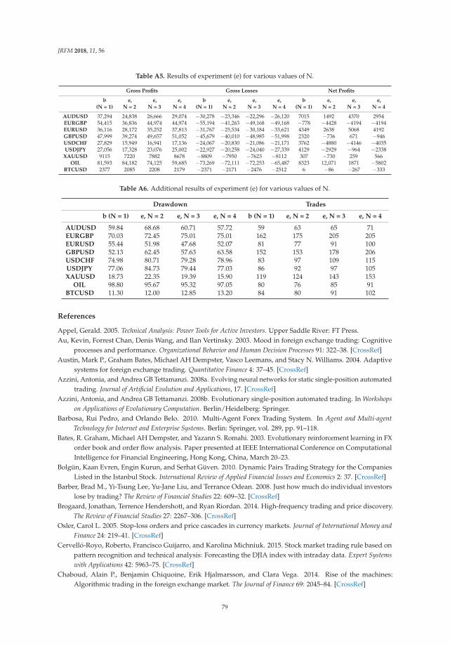
JRFM 2018, 11, 56
Table A5. Results of experiment (e) for various values of N.
Gross Profits Gross Losses Net Profits
b(N = 1)
e,N = 2
e,N = 3
e,N = 4
b(N = 1)
e,N = 2
e,N = 3
e,N = 4
b(N = 1)
e,N = 2
e,N = 3
e,N = 4
AUDUSD 37,294 24,838 26,666 29,074 −30,278 −23,346 −22,296 −26,120 7015 1492 4370 2954EURGBP 54,415 36,836 44,974 44,974 −55,194 −41,263 −49,168 −49,168 −778 −4428 −4194 −4194EURUSD 36,116 28,172 35,252 37,813 −31,767 −25,534 −30,184 −33,621 4349 2638 5068 4192GBPUSD 47,999 39,274 49,657 51,052 −45,679 −40,010 −48,985 −51,998 2320 −736 671 −946USDCHF 27,829 15,949 16,941 17,136 −24,067 −20,830 −21,086 −21,171 3762 −4880 −4146 −4035USDJPY 27,056 17,328 23,076 25,002 −22,927 −20,258 −24,040 −27,339 4129 −2929 −964 −2338
XAUUSD 9115 7220 7882 8678 −8809 −7950 −7623 −8112 307 −730 259 566OIL 81,593 84,182 74,125 59,685 −73,269 −72,111 −72,253 −65,487 8323 12,071 1871 −5802
BTCUSD 2377 2085 2208 2179 −2371 −2171 −2476 −2512 6 −86 −267 −333
Table A6. Additional results of experiment (e) for various values of N.
Drawdown Trades
b (N = 1) e, N = 2 e, N = 3 e, N = 4 b (N = 1) e, N = 2 e, N = 3 e, N = 4
AUDUSD 59.84 68.68 60.71 57.72 59 63 65 71EURGBP 70.03 72.45 75.01 75.01 162 175 205 205EURUSD 55.44 51.98 47.68 52.07 81 77 91 100GBPUSD 52.13 62.45 57.63 63.58 152 153 178 206USDCHF 74.98 80.71 79.28 78.96 83 97 109 115USDJPY 77.06 84.73 79.44 77.03 86 92 97 105XAUUSD 18.73 22.35 19.39 15.90 119 124 143 153
OIL 98.80 95.67 95.32 97.05 80 76 85 91BTCUSD 11.30 12.00 12.85 13.20 84 80 91 102
References
Appel, Gerald. 2005. Technical Analysis: Power Tools for Active Investors. Upper Saddle River: FT Press.Au, Kevin, Forrest Chan, Denis Wang, and Ilan Vertinsky. 2003. Mood in foreign exchange trading: Cognitive
processes and performance. Organizational Behavior and Human Decision Processes 91: 322–38. [CrossRef]Austin, Mark P., Graham Bates, Michael AH Dempster, Vasco Leemans, and Stacy N. Williams. 2004. Adaptive
systems for foreign exchange trading. Quantitative Finance 4: 37–45. [CrossRef]Azzini, Antonia, and Andrea GB Tettamanzi. 2008a. Evolving neural networks for static single-position automated
trading. Journal of Artificial Evolution and Applications, 17. [CrossRef]Azzini, Antonia, and Andrea GB Tettamanzi. 2008b. Evolutionary single-position automated trading. In Workshops
on Applications of Evolutionary Computation. Berlin/Heidelberg: Springer.Barbosa, Rui Pedro, and Orlando Belo. 2010. Multi-Agent Forex Trading System. In Agent and Multi-agent
Technology for Internet and Enterprise Systems. Berlin: Springer, vol. 289, pp. 91–118.Bates, R. Graham, Michael AH Dempster, and Yazann S. Romahi. 2003. Evolutionary reinforcement learning in FX
order book and order flow analysis. Paper presented at IEEE International Conference on ComputationalIntelligence for Financial Engineering, Hong Kong, China, March 20–23.
Bolgün, Kaan Evren, Engin Kurun, and Serhat Güven. 2010. Dynamic Pairs Trading Strategy for the CompaniesListed in the Istanbul Stock. International Review of Applied Financial Issues and Economics 2: 37. [CrossRef]
Barber, Brad M., Yi-Tsung Lee, Yu-Jane Liu, and Terrance Odean. 2008. Just how much do individual investorslose by trading? The Review of Financial Studies 22: 609–32. [CrossRef]
Brogaard, Jonathan, Terrence Hendershott, and Ryan Riordan. 2014. High-frequency trading and price discovery.The Review of Financial Studies 27: 2267–306. [CrossRef]
Osler, Carol L. 2005. Stop-loss orders and price cascades in currency markets. Journal of International Money andFinance 24: 219–41. [CrossRef]
Cervelló-Royo, Roberto, Francisco Guijarro, and Karolina Michniuk. 2015. Stock market trading rule based onpattern recognition and technical analysis: Forecasting the DJIA index with intraday data. Expert Systemswith Applications 42: 5963–75. [CrossRef]
Chaboud, Alain P., Benjamin Chiquoine, Erik Hjalmarsson, and Clara Vega. 2014. Rise of the machines:Algorithmic trading in the foreign exchange market. The Journal of Finance 69: 2045–84. [CrossRef]
79

JRFM 2018, 11, 56
Challet, Damien, and Ahmed Bel Hadj Ayed. 2014. Do Google Trend data contain more predictability than pricereturns? Available online: https://arxiv.org/abs/1403.1715 (accessed on 24 July 2018).
Chan, Oliver, and Alfred Ka Chun Ma. 2015. A Framework for Stop-Loss Analysis on Trading Strategies.The Journal of Trading 10: 87–95. [CrossRef]
Chevallier, Julien, Wei Ding, and Florian Ielpo. 2012. Implementing a Simple Rule for Dynamic Stop-LossStrategies. The Journal of Investing 21: 111–14. [CrossRef]
Chong, Terence Tai-Leung, and Wing-Kam Ng. 2008. Technical analysis and the London stock exchange: testingthe MACD and RSI rules using the FT30. Applied Economics Letters 15: 1111–14. [CrossRef]
Clare, Andrew, James Seaton, Peter N. Smith, and Stephen Thomas. 2013. Breaking into the blackbox: Trendfollowing, stop losses and the frequency of trading–The case of the S&P500. Journal of Asset Management 14:182–94.
Easley, David, MM Lopez De Prado, and Maureen O’Hara. 2011. The microstructure of the flash crash: Flowtoxicity, liquidity crashes and the probability of informed trading. Journal of Portfolio Management 37: 118–28.[CrossRef]
Foucault, Thierry, Bruno Biais, and Sophie Moinas. 2011. Equilibrium High Frequency Trading. Paper presentedat International Conference of the French Finance Association, Montpellier, France, May 11.
Han, Yufeng, Guofu Zhou, and Yingzi Zhu. 2016. Taming Momentum Crashes: A Simple Stop-LossStrategy. Available online: https://ssrn.com/abstract=2407199 or http://dx.doi.org/10.2139/ssrn.2407199(accessed on 26 July 2018).
Hendershott, Terrence, Charles M. Jones, and Albert J. Menkveld. 2011. Does algorithmic trading improveliquidity? The Journal of Finance 66: 1–33. [CrossRef]
Hendershott, Terrence, and Pam Moulton. 2007. The Shrinking New York Stock Exchange Floor and the Hybrid Market.Technical Report. Berkeley: University of California, Available online: https://docplayer.net/13539804-The-shrinking-new-york-stock-exchange-floor-and-the-hybrid-market.html (accessed on 25 July 2018).
Jain, Pankaj K. 2005. Financial market design and the equity premium: Electronic versus floor trading. The Journalof Finance 60: 2955–85. [CrossRef]
Kaminski, Kathryn, and Andrew W. Lo. 2014. When do stop-loss rules stop losses? Journal of Financial Markets 18:234–54. [CrossRef]
Kaniel, Ron, Saar Gideon, and Titman Sheridan. 2004. Individual Investor Sentiment and Stock Returns. Availableonline: https://ssrn.com/abstract=1294447 (accessed on 24 July 2018).
Klement, Joachim. 2013. Assessing Stop-Loss and Re-Entry Strategies. Available online: https://ssrn.com/abstract=2277722 or http://dx.doi.org/10.2139/ssrn.2277722 (accessed on 26 July 2018).
Lei, Adam YC, and Huihua Li. 2009. The Value of Stop Loss Strategies. Financial Services Review 18: 23–51. [CrossRef]Leung, Tim, and Xin Li. 2015. Optimal mean reversion trading with transaction costs and stop-loss exit.
International Journal of Theoretical and Applied Finance 18: 1550020. [CrossRef]Martinez, Leonardo C., Diego N. da Hora, Joao R. de M. Palotti, Wagner Meira, and Gisele L. Pappa. 2009. From
an artificial neural network to a stock market day-trading system: A case study on the BM&F BOVESPA.Paper presented at International Joint Conference on Neural Networks, Atlanta, GA, USA, June 14–19.
Ni, He, and Hujun Yin. 2009. Exchange rate prediction using hybrid neural networks and trading indicators.Neurocomputing 72: 2815–23. [CrossRef]
Preis, Tobias, Helen Susannah Moat, and H. Eugene Stanley. 2013. Quantifying trading behavior in financialmarkets using Google Trends. Scientific Reports 3: 1684. [CrossRef] [PubMed]
Krishnan, Rajeswari, and S. Sandhya Menon. 2009. Impact of Currency Pairs, Time Frames and TechnicalIndicators on Trading Profit in Forex Spot Market. International Journal of Business Insights & Transformation 2:34–51.
Wilder, J. Welles. 1978. New Concepts in Technical Trading Systems. Chicago: Investor Publishing, Inc.Yazdi, Seyed Hadi Mir, and Ziba Habibi Lashkari. 2013. Technical Analysis of Forex by MACD Indicator.
International Journal of Humanities and Management Sciences 1: 159–65.
© 2018 by the authors. Licensee MDPI, Basel, Switzerland. This article is an open accessarticle distributed under the terms and conditions of the Creative Commons Attribution(CC BY) license (http://creativecommons.org/licenses/by/4.0/).
80

Journal of
Risk and FinancialManagement
Article
Predicting Currency Crises: A Novel ApproachCombining Random Forests and Wavelet Transform
Lei Xu, Takuji Kinkyo and Shigeyuki Hamori *
Graduate School of Economics, Kobe University, 2-1, Rokkodai, Nada-Ku, Kobe 657-8501, Japan;[email protected] (L.X.); [email protected] (T.K.)* Correspondence: [email protected]
Received: 1 November 2018; Accepted: 1 December 2018; Published: 4 December 2018
Abstract: We propose a novel approach that combines random forests and the wavelet transform tomodel the prediction of currency crises. Our classification model of random forests, built usingboth standard predictors and wavelet predictors, and obtained from the wavelet transform, achievesa demonstrably high level of predictive accuracy. We also use variable importance measures tofind that wavelet predictors are key predictors of crises. In particular, we find that real exchangerate appreciation and overvaluation, which are measured over a horizon of 16–32 months, are themost important.
Keywords: currency crisis; random forests; wavelet transform; predictive accuracy
JEL Classification: F31; F37; F47
1. Introduction
Severe economic collapse in developing countries often involves currency crises triggered byspeculative attacks on the currency and sudden stops to capital inflows. An unexpectedly sharpexchange rate depreciation tends to have a contractionary effect on economic activities, owing to anextensive dollarization of liabilities in both bank and corporate balance sheets. Thus, preventing seriouscurrency crises is considered a priority task of macroeconomic management in developing countries.
Having observed the severe economic consequences of emerging market currency crises duringthe 1990s, economists have searched for a reliable currency crisis prediction model. The seminalworks include Frankel and Rose (1996) and Kaminsky et al. (1998). Frankel and Rose (1996) definea currency crash as the nominal depreciation of a currency’s value by at least 25%, which is also atleast a 10% increase in the rate of depreciation. They estimate multivariate logistic regressions andfind that a currency crash tends to occur when output growth is low, the growth of domestic creditis high, and the foreign interest level is high. Kaminsky et al. (1998) propose a signaling approach,which seeks to identify the threshold values for individual predictors. They find that exports, realexchange rate overvaluation, GDP growth, foreign exchange reserves, and equity prices are the mostreliable predictors of crises. Berg and Pattillo (1999) use panel probit models and show that theirforecasting ability outperforms the signaling approach. Bussiere and Fratzscher (2006) use multinomiallogistic regressions, which distinguish between tranquil periods, crisis periods, and post-crisis periods.They use the exchange market pressure (EMP) index originally proposed by Eichengreen et al. (1995)to define a currency crisis and show that the multinomial logistic model predicts crises better thanthe binomial logistic model. In a similar vein, Abiad (2003) and Peria (2002) use a Markov-switchingmodel, which identifies and characterizes crisis periods endogenously. Shimpalee and Breuer (2006)focus on the role of institutional factors and use the probit model to show that corruption, de facto fixedexchange rates, weak government stability, and weak law and order increase the probability of crises.
JRFM 2018, 11, 86; doi:10.3390/jrfm11040086 www.mdpi.com/journal/jrfm81
JRFM 2018, 11, 86
The global financial crisis of 2008 has rekindled interest in this topic. Rose and Spiegel (2011, 2012)regressed the measure of crisis intensity on a set of potential predictors; however, they found fewclear and reliable predictors for the cross-country incidence of severe recessions during the globalfinancial crisis. Frankel and Frankel and Saravelos (2012) investigated whether traditional indicatorscan help explain why some countries were badly impacted by the global financial crisis and foundthat foreign exchange reserves and real exchange rate overvaluation are the most useful predictors.Gourinchas and Obstfeld (2012) employed the methods of event studies and logit regressions andfound that domestic credit expansion, real exchange rate appreciation, and foreign exchange reservesare useful predictors of crises in emerging market economies. Sevim et al. (2014) used decision treesand artificial neural networks to predict currency crises in Turkey and showed that results from thesetwo methods are superior to those obtained by logistic regressions.
In this study, we propose a novel approach that combines a machine learning technique of randomforests and a signal processing method of the wavelet transform to model the prediction of currencycrises. We demonstrate that our model can achieve a high level of accuracy in predicting currencycrises. Our contribution to the literature is two-fold. First, we use the wavelet transform to extractkey features of exchange rate behavior that may signal the risk of currency crises. The existing studiestend to focus on a particular aspect of exchange rate behavior, such as overvaluation or volatility overa particular period of time. By applying the wavelet transform, we can systemically extract variousfeatures of exchange rate behavior across different time horizons. Recent literature in economics andfinance makes extensive use of wavelet analysis, indicating its usefulness as a tool for feature extraction(Reboredo and Rivera-Castro 2013; Cai et al. 2017; Faria and Verona 2018). Second, we constructa prediction model by applying the random forests method, which is a variant of decision trees.The existing literature is generally more concerned with identifying the key predictors of crises thanimproving the predictive accuracy (Frankel and Saravelos 2012). We choose the random forestsmethod to construct a prediction model because it can significantly improve predictive accuracyby building a large number of trees using random input selection (Breiman 2001). In addition,the random forests method provides variable importance measures that rank predictors according totheir contribution to the prediction. Thus, the random forests method also addresses the traditionalquestion of which predictors are most reliable. Owing to its superior performance, the randomforests method has been increasingly employed in the area of economic and financial forecasting(Tanaka et al. 2018).
The rest of the paper is organized as follows. In Section 2, we explain the methodology andthe data. In Section 3, we evaluate the predictive accuracy of the models and present the variableimportance measures. Section 4 provides our conclusions.
2. Methodology and Data
2.1. Discrete Wavelet Transformation
We applied the discrete wavelet transform (DWT) to a time series of monthly exchange rates andsystemically extracted key features of exchange rate behavior over different time horizons. Specifically,we used a modified version of DWT known as the maximal overlap DWT (MODWT) because its samplesize need not be restricted to a power of two. Existing studies typically measure the deviation from thetrend and the volatility of exchange rates over an arbitrarily selected period of time. Our approach hasan advantage over the existing methods because it evaluates various aspects of exchange rate behaviorover different time horizons. The MODWT was computed using the pyramid algorithm proposed byPercival and Walden (2000)1.
1 The computation of the MODWT is conducted using the “Wavelets” package in the R software package.
82
JRFM 2018, 11, 86
The sample variance of the exchange rate series can be decomposed into parts corresponding tothe variance of the series on different scales. For a partial DWT of level J0, the decomposition isgiven by:
σ2X =
1N
J0
∑j=1
∥∥∥Wj
∥∥∥2+
1N‖VJ0‖
2 − X2, (1)
where σ2X denotes the sample variance of the exchange rate series; Wj denotes an N dimensional
vector, whose element Wj,t is the jth level wavelet coefficient corresponding to a scale of τj = 2j−1;VJ0 denotes an N dimensional column vector, whose element VJ0,t is the J0th level scaling coefficientcorresponding to a scale of λj = 2j; and X denotes the sample average of the exchange rate series2.The jth level wavelet coefficients of Wj and the scaling coefficients of VJ0 are given by:
Wj = BjVj−1 = Bj Aj−1 · · · A1X, (2)
VJ0 = AJ0 VJ0−1 = AJ0 AJ0−1 · · · A1X, (3)
where Bj and Aj are N × N matrices whose rows contain circularly shifted and up-sampled versions ofthe wavelet filter, {hl}, and scaling filter, {gl}, periodized to length N; N denotes the sample size;and X denotes an N dimensional vector, whose element {Xt} is the exchange rate series3.
The multi-resolution analysis (MRA) decomposes a time series of exchange rates into partscorresponding to the variation of the series on different scales. For a partial DWT of level J0, the MRAis given by:
X =J0
∑j=1
Dj + SJ0 , (4)
where Dj denotes an N dimensional vector whose element Dj,t is the jth level wavelet detailcorresponding to a scale, τj = 2j−1, and SJ0 denotes an N dimensional vector, whose element SJ0,t isthe J0th level smooth function corresponding to a scale, λj = 2j. The jth level details of Dj and thesmooth function of SJ0 are given by:
Dj = AT1 · · · AT
j−1BTj Wj (5)
andSJ0 = AT
1 · · · ATJ0−1 AT
J0VJ0 , (6)
respectively, where BTj and AT
j denote the transposers of Bj and Aj, respectively4.
A cascade of wavelet filters relating Wj,t to Xt is an approximation to a band-pass filterwith the pass-band given by [1/2j+1, 1/2j], while a cascade of scaling filters relating Vj,t to Xt isan approximation to a low-pass filter with the pass-band given by [0, 1/2j+1]. Correspondingly,Dj,t represents the variation of monthly exchange rates over 2j − 2j+1 months, while Sj,t represents thetrend obtained after the sum of Dj,t, up to the jth level, is removed from the series.
2 Equation (1) is derived from the energy preserving condition: ‖X‖2 =J0∑
j=1
∥∥∥Wj
∥∥∥2+ ‖VJ0‖
2.
3 While Fourier transform coefficients are associated with frequencies, wavelet coefficients are associated with a particularscale and set of times.
4 Using the orthonormality of DWT, the MRA is obtained by pre-multiplying both sides of Equations (2) and (3) by thetransposer of Bj Aj−1 · · · A1 and AJ0 AJ0−1 · · · A1, respectively.
83
JRFM 2018, 11, 86
We set J0 = 5 and computed each level of Wj,t, Vj,t, Dj,t, and Sj,t up to the fifth level. Our choice ofMODWT wavelet and scaling filters are Harr filters5, which are given by:
h0 = 1/2, h1 = −1/2, g0 = 1/2, g1 = −1/2. (7)
We used a time series of Wj,t, Vj,t, Dj,t, and Sj,t as predictors for building a classificationmodel of random forests. Specifically, we used the square of Wj,t and Vj,t to capture the scale-by-scalecontribution to the volatility of nominal exchange rates, while we used Dj,t to capture the variation ofreal exchange rates over various time horizons. In addition, we measured the overvaluation of realexchange rates by computing the difference between the actual value of the real exchange rates and thecorresponding Sj,t on each scale. The nominal exchange rate was the end-of-period monthly bilateraldollar exchange rate, while the real exchange rate is computed by deflating the nominal exchange ratewith the consumer price index (CPI). Both nominal and real exchange rates were transformed intologarithmic terms.
2.2. The EMP Index
A currency crisis can be characterized as a situation in which a country’s currency is under asevere attack that leads to a sharp depreciation of exchange rates and/or a substantial loss in foreignexchange reserves. To measure the extent of downward pressures on exchange rates, many studiesemploy the EMP index originally proposed by Eichengreen et al. (1995). In this study, we used themodified version of the EMP index employed by Bussiere and Fratzscher (2006). The modified indexis the weighted average of the annual changes of real exchange rates and foreign exchange reservesgiven by:6
EMPi,t = ωexr
(rexri,t − rexri,t−1
rexri,t−1
)− ωresr
(resi,t − resi,t−1
resi,t−1
), (8)
where rexri,t denotes the real exchange rate as defined above; resi,t denotes the foreign exchangereserves; ωexr and ωresr denote the inverse of the variance of change rates in exchange rates andforeign exchange reserves, respectively; and the subscripts i and t denote a specific country and time,respectively. Using this EMP index, a binary variable of currency crises is defined as follows:
Crisisi,t =
{1 if EMPi,t > μEMPi,t + 2σEMPi,t
0 otherwise, (9)
where μEMPi,t and σEMPi,t denote the sample mean and the standard deviation of the EMP index,respectively, for each country.
Table 1 shows the number of currency crises obtained during the sample period by usingEquation (9).
5 In addition to the Harr filter, we also used LA8 and D4 to derive wavelet predictors and evaluate the predictive accuracy.The reason we have chosen to use the Harr filter is because it is the only filter that produces consistent results. When weused LA8 and D4, the random forests method performed better than the logistic regression based on the balanced accuracyand the F-measure, while the latter performed better than the former based on AUC. By contrast, the random forests methodconsistently outperformed the logistic regression when the Harr filter was used.
6 Although the original index also includes interest rate differentials, Kaminsky et al. (1998) removed it from their indexbecause developing countries often adopt interest rate control. Since our sample includes many developing countries,we exclude interest rate differentials from the index. Note also that real exchange rates are used instead of nominal exchangerates to take into account differences in inflation rates across countries.
84
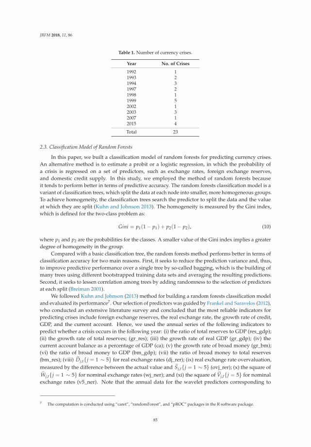
JRFM 2018, 11, 86
Table 1. Number of currency crises.
Year No. of Crises
1992 11993 21994 31997 21998 11999 52002 12003 32007 12015 4
Total 23
2.3. Classification Model of Random Forests
In this paper, we built a classification model of random forests for predicting currency crises.An alternative method is to estimate a probit or a logistic regression, in which the probability ofa crisis is regressed on a set of predictors, such as exchange rates, foreign exchange reserves,and domestic credit supply. In this study, we employed the method of random forests becauseit tends to perform better in terms of predictive accuracy. The random forests classification model is avariant of classification trees, which split the data at each node into smaller, more homogeneous groups.To achieve homogeneity, the classification trees search the predictor to split the data and the valueat which they are split (Kuhn and Johnson 2013). The homogeneity is measured by the Gini index,which is defined for the two-class problem as:
Gini = p1(1 − p1) + p2(1 − p2), (10)
where p1 and p2 are the probabilities for the classes. A smaller value of the Gini index implies a greaterdegree of homogeneity in the group.
Compared with a basic classification tree, the random forests method performs better in terms ofclassification accuracy for two main reasons. First, it seeks to reduce the prediction variance and, thus,to improve predictive performance over a single tree by so-called bagging, which is the building ofmany trees using different bootstrapped training data sets and averaging the resulting predictions.Second, it seeks to lessen correlation among trees by adding randomness to the selection of predictorsat each split (Breiman 2001).
We followed Kuhn and Johnson (2013) method for building a random forests classification modeland evaluated its performance7. Our selection of predictors was guided by Frankel and Saravelos (2012),who conducted an extensive literature survey and concluded that the most reliable indicators forpredicting crises include foreign exchange reserves, the real exchange rate, the growth rate of credit,GDP, and the current account. Hence, we used the annual series of the following indicators topredict whether a crisis occurs in the following year: (i) the ratio of total reserves to GDP (res_gdp);(ii) the growth rate of total reserves; (gr_res); (iii) the growth rate of real GDP (gr_gdp); (iv) thecurrent account balance as a percentage of GDP (ca); (v) the growth rate of broad money (gr_bm);(vi) the ratio of broad money to GDP (bm_gdp); (vii) the ratio of broad money to total reserves(bm_res); (viii) Dj,t{j = 1 ∼ 5} for real exchange rates (dj_rer); (ix) real exchange rate overvaluation,measured by the difference between the actual value and Sj,t{j = 1 ∼ 5} (ovj_rer); (x) the square ofWj,t{j = 1 ∼ 5} for nominal exchange rates (wj_ner); and (xi) the square of Vj,t{j = 5} for nominalexchange rates (v5_ner). Note that the annual data for the wavelet predictors corresponding to
7 The computation is conducted using “caret”, “randomForest”, and “pROC” packages in the R software package.
85
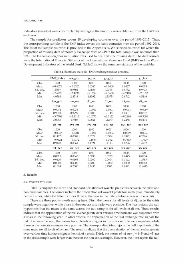
JRFM 2018, 11, 86
indicators (viii)–(xi) were constructed by averaging the monthly series obtained from the DWT foreach year.
The sample for predictors covers 40 developing countries over the period 1991–2015. Thus,the corresponding sample of the EMP index covers the same countries over the period 1992–2016.The list of the sample countries is provided in the Appendix A. We selected countries for which theproportion of missing data of monthly exchange rates or CPI in the total sample was not more than10%. The k-nearest-neighbor imputation was used to deal with the missing data. The data sourceswere the International Financial Statistics of the International Monetary Fund (IMF) and the WorldDevelopment Indicators of the World Bank. Table 2 shows the summary statistics of the variables.
Table 2. Summary statistics. EMP: exchange market pressure.
EMP_index res_gdp gr_res gr_gdp ca gr_bm
Obs. 1000 1000 1000 1000 1000 1000Mean −0.4671 −0.0025 0.0165 −0.0009 0.0037 0.0013
Sd. dev. 1.5397 0.9801 0.9856 0.9795 0.9752 0.9773Min −7.6276 −2.4292 −2.8799 −4.3650 −4.2418 −2.1852Max 4.9584 2.8716 4.6392 4.3375 2.8742 4.5146
bm_gdp bm_res d1_rer d2_rer d3_rer d4_rer
Obs. 1000 1000 1000 1000 1000 1000Mean 0.0044 0.0035 −0.0001 −0.0001 −0.0001 −0.0007
Sd. dev. 0.9813 0.9799 0.0088 0.0148 0.0351 0.0837Min −3.7706 −2.1113 −0.0772 −0.1122 −0.2180 −0.5096Max 3.0995 4.7506 0.0861 0.1279 0.2288 0.5434
d5_rer ov1_rer ov2_rer ov3_rer ov4_rer ov5_rer
Obs. 1000 1000 1000 1000 1000 1000Mean −0.0037 −0.0001 −0.0001 −0.0002 −0.0009 −0.0046
Sd. dev. 0.1417 0.0088 0.0229 0.0554 0.1342 0.2586Min −0.9524 −0.0772 −0.1684 −0.3621 −0.7815 −1.7339Max 0.9170 0.0861 0.1924 0.4113 0.8296 1.4932
w1_ner w2_ner w3_ner w4_ner w5_ner v5_ner
Obs. 1000 1000 1000 1000 1000 1000Mean 0.0025 0.0047 0.0098 0.0208 0.0445 0.8894
Sd. dev. 0.0120 0.0165 0.0300 0.0604 0.1142 1.2783Min 0.0000 0.0000 0.0000 0.0000 0.0000 0.0000Max 0.1614 0.2000 0.3433 0.7592 1.0942 10.6675
3. Results
3.1. Wavelet Predictors
Table 3 compares the mean and standard deviations of wavelet predictors between the crisis andnon-crisis samples. The former includes the observations of wavelet predictors in the year immediatelybefore a crisis, while the latter includes those in the year immediately before a year with no crisis.
There are three points worth noting here. First, the means for all levels of dj_rer in the crisissample were negative, while those in the non-crisis sample were positive. The t-test rejects the nullhypothesis that the mean is the same across the two samples for all levels of dj_rer. These resultsindicate that the appreciation of the real exchange rate over various time horizons was associated witha crisis in the following year. In other words, the appreciation of the real exchange rate signals therisk of a crisis. Second, the means for all levels of ovj_rer in the crisis sample were negative, whilethose in the non-crisis sample were positive. The corresponding t-test rejects the null hypothesis of thesame mean for all levels of ovj_rer. The results indicate that the overvaluation of the real exchange rateover various time horizons signals the risk of a crisis. Third, the means of wj_ner (j = 1~5) and v5_nerin the crisis sample were larger than those in the non-crisis sample. However, the t-test rejects the null
86
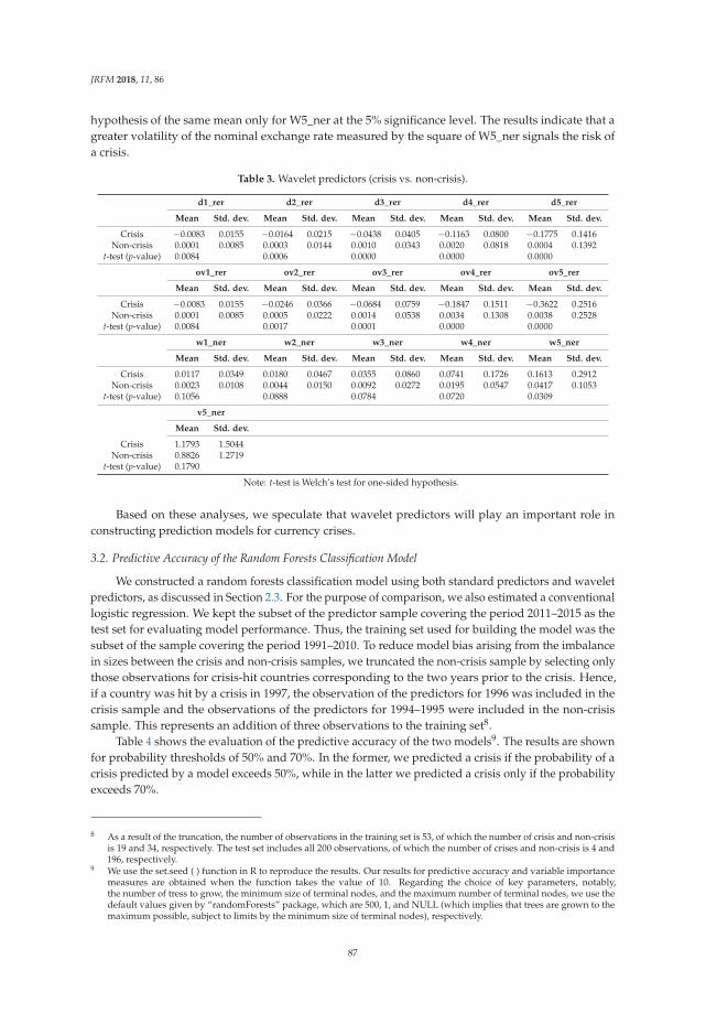
JRFM 2018, 11, 86
hypothesis of the same mean only for W5_ner at the 5% significance level. The results indicate that agreater volatility of the nominal exchange rate measured by the square of W5_ner signals the risk ofa crisis.
Table 3. Wavelet predictors (crisis vs. non-crisis).
d1_rer d2_rer d3_rer d4_rer d5_rer
Mean Std. dev. Mean Std. dev. Mean Std. dev. Mean Std. dev. Mean Std. dev.
Crisis −0.0083 0.0155 −0.0164 0.0215 −0.0438 0.0405 −0.1163 0.0800 −0.1775 0.1416Non-crisis 0.0001 0.0085 0.0003 0.0144 0.0010 0.0343 0.0020 0.0818 0.0004 0.1392
t-test (p-value) 0.0084 0.0006 0.0000 0.0000 0.0000
ov1_rer ov2_rer ov3_rer ov4_rer ov5_rer
Mean Std. dev. Mean Std. dev. Mean Std. dev. Mean Std. dev. Mean Std. dev.
Crisis −0.0083 0.0155 −0.0246 0.0366 −0.0684 0.0759 −0.1847 0.1511 −0.3622 0.2516Non-crisis 0.0001 0.0085 0.0005 0.0222 0.0014 0.0538 0.0034 0.1308 0.0038 0.2528
t-test (p-value) 0.0084 0.0017 0.0001 0.0000 0.0000
w1_ner w2_ner w3_ner w4_ner w5_ner
Mean Std. dev. Mean Std. dev. Mean Std. dev. Mean Std. dev. Mean Std. dev.
Crisis 0.0117 0.0349 0.0180 0.0467 0.0355 0.0860 0.0741 0.1726 0.1613 0.2912Non-crisis 0.0023 0.0108 0.0044 0.0150 0.0092 0.0272 0.0195 0.0547 0.0417 0.1053
t-test (p-value) 0.1056 0.0888 0.0784 0.0720 0.0309
v5_ner
Mean Std. dev.
Crisis 1.1793 1.5044Non-crisis 0.8826 1.2719
t-test (p-value) 0.1790
Note: t-test is Welch’s test for one-sided hypothesis.
Based on these analyses, we speculate that wavelet predictors will play an important role inconstructing prediction models for currency crises.
3.2. Predictive Accuracy of the Random Forests Classification Model
We constructed a random forests classification model using both standard predictors and waveletpredictors, as discussed in Section 2.3. For the purpose of comparison, we also estimated a conventionallogistic regression. We kept the subset of the predictor sample covering the period 2011–2015 as thetest set for evaluating model performance. Thus, the training set used for building the model was thesubset of the sample covering the period 1991–2010. To reduce model bias arising from the imbalancein sizes between the crisis and non-crisis samples, we truncated the non-crisis sample by selecting onlythose observations for crisis-hit countries corresponding to the two years prior to the crisis. Hence,if a country was hit by a crisis in 1997, the observation of the predictors for 1996 was included in thecrisis sample and the observations of the predictors for 1994–1995 were included in the non-crisissample. This represents an addition of three observations to the training set8.
Table 4 shows the evaluation of the predictive accuracy of the two models9. The results are shownfor probability thresholds of 50% and 70%. In the former, we predicted a crisis if the probability of acrisis predicted by a model exceeds 50%, while in the latter we predicted a crisis only if the probabilityexceeds 70%.
8 As a result of the truncation, the number of observations in the training set is 53, of which the number of crisis and non-crisisis 19 and 34, respectively. The test set includes all 200 observations, of which the number of crises and non-crisis is 4 and196, respectively.
9 We use the set.seed ( ) function in R to reproduce the results. Our results for predictive accuracy and variable importancemeasures are obtained when the function takes the value of 10. Regarding the choice of key parameters, notably,the number of tress to grow, the minimum size of terminal nodes, and the maximum number of terminal nodes, we use thedefault values given by “randomForests” package, which are 500, 1, and NULL (which implies that trees are grown to themaximum possible, subject to limits by the minimum size of terminal nodes), respectively.
87

JRFM 2018, 11, 86
Table 4. Predictive accuracy of the models. AUC: area under the receiver operating characteristic curve.
50% Threshold 70% Threshold
Random Forests Logistic Regression Random Forests Logistic Regression
Sensitivity 0.9565 0.8696 0.8696 0.8696Specificity 0.8608 0.8270 0.9222 0.8301
Balanced accuracy 0.9087 0.8483 0.8959 0.8499F-measure 0.9061 0.8478 0.8951 0.8494
Random Forests Logistic Regression
AUC 0.9496 0.857
The sensitivity is defined as the ratio that a crisis is predicted accurately for all samples having acrisis event, and is given by:
sensitivity =samples with a crisis event and predicted to have a crisis
samples with a crisis event.
The sensitivity is synonymous with the true-positive rate. By contrast, the specificity is definedas the ratio that a non-crisis is predicted accurately for all samples without a crisis event, which isgiven by:
specificity =samples without a crisis event and predicted to have no crisis
samples without a crisis event.
The false-positive rate is defined as one minus the specificity. Since there tends to be a trade-offbetween the sensitivity and the specificity, the balanced accuracy and the F-measure are often used toevaluate the overall accuracy. The former is the arithmetic mean of the sensitivity and the specificity,while the latter is the harmonic mean. As can be seen from the table, the levels of sensitivity, specificity,balanced accuracy, and the F-measure are fairly high for both the random forests method and thelogistic regression. Overall, the random forests method performs better than the logistic regressionin terms of classification accuracy. Note that both the balanced accuracy and the F-measure for therandom forests method exceed 0.9 based on the 50% threshold.
We also used a receiver operating characteristic (ROC) curve to evaluate the predictive accuracy ofthe models. A ROC curve was constructed by plotting the true-positive rate and the false-positiverate against each other for each candidate threshold. The measure of the overall performance of themodel was given by the area under the ROC curve (AUC). A larger value of AUC implies a betterpredictive performance of the model. The level of AUC was fairly high for both the random forestsand the logistic regression, and the former performed better than the latter in terms of overall accuracy.
3.3. Variable Importance Measures
A valuable property of the random forests method is that it provides variable importance measuresthat rank predictors according to their contribution to the prediction. The variable importance measurewas calculated by adding up the total reduction in the Gini index by splits over a given predictor,averaged over all bagged trees.
Figure 1 shows the variable importance measure for each predictor. Among the range of waveletpredictors, ov4_rer and d4_rer are the most important crisis predictors. The result is in line withthe existing literature that emphasizes the importance of the real exchange rate overvaluation insignaling the risk of currency crises (see, for example, Kaminsky et al. 1998; Frankel and Saravelos 2012;Gourinchas and Obstfeld 2012). The remaining top five predictors include ov3_rer, d3_rer, and w5_ner.It is worth noting that the volatility of nominal exchange rates is also an important crisis predictor.In contrast to common perception, the level of foreign exchange reserves or the growth rate of domesticcredit are less important crisis predictors in our model.
88
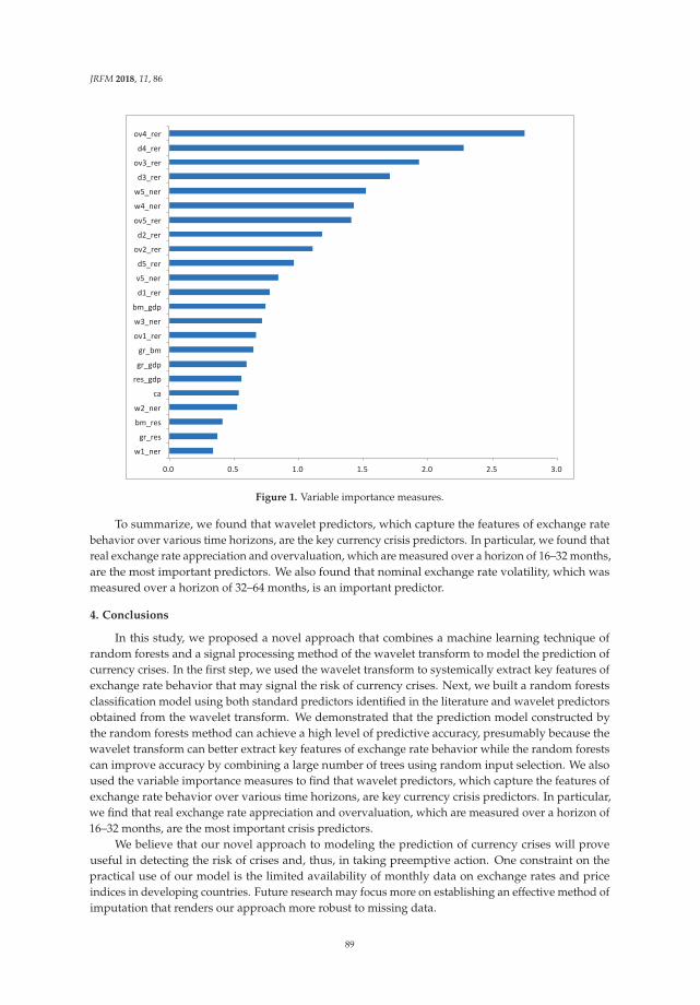
JRFM 2018, 11, 86
0.0 0.5 1.0 1.5 2.0 2.5 3.0
w1_ner
gr_res
bm_res
w2_ner
ca
res_gdp
gr_gdp
gr_bm
ov1_rer
w3_ner
bm_gdp
d1_rer
v5_ner
d5_rer
ov2_rer
d2_rer
ov5_rer
w4_ner
w5_ner
d3_rer
ov3_rer
d4_rer
ov4_rer
Figure 1. Variable importance measures.
To summarize, we found that wavelet predictors, which capture the features of exchange ratebehavior over various time horizons, are the key currency crisis predictors. In particular, we found thatreal exchange rate appreciation and overvaluation, which are measured over a horizon of 16–32 months,are the most important predictors. We also found that nominal exchange rate volatility, which wasmeasured over a horizon of 32–64 months, is an important predictor.
4. Conclusions
In this study, we proposed a novel approach that combines a machine learning technique ofrandom forests and a signal processing method of the wavelet transform to model the prediction ofcurrency crises. In the first step, we used the wavelet transform to systemically extract key features ofexchange rate behavior that may signal the risk of currency crises. Next, we built a random forestsclassification model using both standard predictors identified in the literature and wavelet predictorsobtained from the wavelet transform. We demonstrated that the prediction model constructed bythe random forests method can achieve a high level of predictive accuracy, presumably because thewavelet transform can better extract key features of exchange rate behavior while the random forestscan improve accuracy by combining a large number of trees using random input selection. We alsoused the variable importance measures to find that wavelet predictors, which capture the features ofexchange rate behavior over various time horizons, are key currency crisis predictors. In particular,we find that real exchange rate appreciation and overvaluation, which are measured over a horizon of16–32 months, are the most important crisis predictors.
We believe that our novel approach to modeling the prediction of currency crises will proveuseful in detecting the risk of crises and, thus, in taking preemptive action. One constraint on thepractical use of our model is the limited availability of monthly data on exchange rates and priceindices in developing countries. Future research may focus more on establishing an effective method ofimputation that renders our approach more robust to missing data.
89

JRFM 2018, 11, 86
Author Contributions: S.H. and T.K. conceived and designed the experiments; L.X. performed the experiments,analyzed the data, and contributed reagents/materials/analysis tools; L.X., S.H., and T.K. wrote the paper.
Funding: This research was supported by JSPS KAKENHI Grant Number 17K18564, (A) 17H00983, and 18K01610.
Acknowledgments: We are grateful to two anonymous referees for their helpful comments and suggestions.
Conflicts of Interest: The authors declare no conflict of interest. The founding sponsors had no role in thedesign of the study, in the collection, analyses, or interpretation of data, in the writing of the manuscript, or in thedecision to publish the results.
Appendix A. List of Sample Countries
Algeria, Bulgaria, Burundi, Cabo Verde, Central African Republic, Chad, Chile, China, Colombia,Dominican Republic, Egypt, Equatorial Guinea, Gabon, Gambia, Guatemala, Honduras, Hungary,Kenya, Madagascar, Malawi, Malaysia, Mauritius, Mexico, Namibia, Nigeria, Peru, Philippines, Poland,Romania, Seychelles, South Africa, Sri Lanka, Sudan, Thailand, Tunisia, Turkey, Uganda, Uruguay,Venezuela, Zambia.
References
Abiad, Abdul. 2003. Early Warning Systems: A Survey and a Regime Switching Approach. IMF Working paperNo. 03/23, International Monetary Fund, Washington, DC, USA.
Berg, Andrew, and Catherine Pattillo. 1999. Predicting currency crises: The indicator approach and an alternative.Journal of International Money and Finance 18: 561–86. [CrossRef]
Breiman, Leo. 2001. Random forests. Machine Learning 45: 5–32. [CrossRef]Bussiere, Matthieu, and Marcel Fratzscher. 2006. Towards a new early warning system of financial crises. Journal of
International Money and Finance 25: 953–73. [CrossRef]Cai, Xiao Jing, Shuairu Tian, Nannan Yuan, and Shigeyuki Hamori. 2017. Interdependence between Oil and East
Asian Stock Markets: Evidence from Wavelet Coherence Analysis. Journal of International Financial Markets,Institutions and Money 48: 206–23. [CrossRef]
Eichengreen, Barry, Andrew K. Rose, and Charles Wyplosz. 1995. Exchange market mayhem: The antecedentsand aftermath of speculative arracks. Economic Policy 21: 249–312. [CrossRef]
Faria, Gonçalo, and Fabio Verona. 2018. Forecasting stock market returns by summing the frequency decomposedparts. Journal of Empirical Finance 45: 228–42. [CrossRef]
Frankel, Jeffrey A., and Andrew K. Rose. 1996. Currency crashes in emerging markets: An empirical treatment.Journal of International Economics 41: 351–66. [CrossRef]
Frankel, Jeffrey, and George Saravelos. 2012. Can leading indicators assess country vulnerability? Evidence fromthe 2008–2009 global financial crisis. Journal of International Economics 87: 216–31. [CrossRef]
Gourinchas, Pierre-Olivier, and Maurice Obstfeld. 2012. Stories of the twentieth century for the twenty-first.American Economic Journal: Macroeconomics 4: 226–65. [CrossRef]
Kaminsky, Graciela, Saul Lizondo, and Carmen M. Reinhart. 1998. The leading indicators of currency crises.IMF Staff Paper 45: 1–48. [CrossRef]
Kuhn, Max, and Kjell Johnson. 2013. Applied Predictive Modeling. New York: Springer.Percival, Donald B., and Andrew T. Walden. 2000. Wavelet Methods for Time Series Analysis. Cambridge:
Cambridge University Press.Peria, Maria Soledad Martinez. 2002. A regime-switching approach to the study of speculative attacks: A focus on
EMS crises. Empirical Economics 27: 299–334. [CrossRef]Reboredo, Juan C., and Miguel A. Rivera-Castro. 2013. A Wavelet decomposition approach to crude oil price and
exchange rate dependence. Economic Modelling 32: 42–57. [CrossRef]Rose, Andrew K., and Mark M. Spiegel. 2011. Cross-country causes and consequences of the crisis: An update.
European Economic Review 55: 309–24. [CrossRef]Rose, Andrew K., and Mark M. Spiegel. 2012. Cross-country causes and consequences of the 2008 crisis:
Early warning. Japan and the World Economy 24: 1–16. [CrossRef]Sevim, Cuneyt, Asil Oztekin, Ozkan Bali, Serkan Gumus, and Erkam Guresen. 2014. Developing an early warning
system to predict currency crises. European Journal of Operational Research 237: 1095–104. [CrossRef]
90

JRFM 2018, 11, 86
Shimpalee, Pattama L., and Janice Boucher Breuer. 2006. Currency crises and institutions. Journal of InternationalMoney and Finance 25: 125–45. [CrossRef]
Tanaka, Katsuyuki, Takuji Kinkyo, and Shigeyuki Hamori. 2018. Financial hazard map: Financial vulnerabilitypredicted by a random forests classification model. Sustainability 10: 1530. [CrossRef]
© 2018 by the authors. Licensee MDPI, Basel, Switzerland. This article is an open accessarticle distributed under the terms and conditions of the Creative Commons Attribution(CC BY) license (http://creativecommons.org/licenses/by/4.0/).
91

Journal of
Risk and FinancialManagement
Article
Predicting Micro-Enterprise Failures Using DataMining Techniques
Aneta Ptak-Chmielewska
Institute of Statistics and Demography, Warsaw School of Economics, Warsaw 02-554, Poland;[email protected]; Tel.: +48-22-564-92-70
Received: 30 December 2018; Accepted: 3 February 2019; Published: 10 February 2019
Abstract: Research analysis of small enterprises are still rare, due to lack of individual leveldata. Small enterprise failures are connected not only with their financial situation abut also withnon-financial factors. In recent research we tend to apply more and more complex models. However,it is not so obvious that increasing complexity increases the effectiveness. In this paper the sample of806 small enterprises were analyzed. Qualitative factors were used in modeling. Some simple andmore complex models were estimated, such as logistic regression, decision trees, neural networks,gradient boosting, and support vector machines. Two hypothesis were verified: (i) not only financialratios but also non-financial factors matter for small enterprise survival, and (ii) advanced statisticalmodels and data mining techniques only insignificantly increase the prediction accuracy of smallenterprise failures. Results show that simple models are as good as more complex model. Datamining models tend to be overfitted. Most important financial ratios in predicting small enterprisefailures were: operating profitability of assets, current assets turnover, capital ratio, coverage ofshort-term liabilities by equity, coverage of fixed assets by equity, and the share of net financialsurplus in total liabilities. Among non-financial factors only two of them were important: the sectorof activity and employment.
Keywords: data mining; bankruptcy prediction; financial and non-financial variables
1. Introduction
Since the announcement of the Altman’s Z-Score model (Altman 1968), a large number ofstatistical bankruptcy prediction studies were written using the traditional methods, like discriminantanalysis (Back et al. 1996), logistic regression (Aziz and Dar 2006; Back et al. 1996), and probit analysis(Zmijewski 1984). Recent studies in this area focus on more advanced and sophisticated methods, likecase-based reasoning (Sartori et al. 2016), genetic algorithms (Back et al. 1996), and neural networks(Blanco-Oliver et al. 2013) or support vector machines (Kim and Sohn 2010).
Sartori et al. (2016) applied the case-based reasoning (CBR) paradigm to forecast the bankruptcyand compared the results received with the Z-Score model. The CBR method turned out to be good inpredicting bankruptcy. The authors found that this approach could be useful to cluster enterprisesaccording to opportune similarity metrics.
Genetic algorithms (GAs) were another method used in SMEs’ default prediction analysis. Gordini(2014) compared the potential of genetic algorithms with two other methods: logistic regression (LR)and support vector machine (SVM). The results obtained suggest that GAs are a very effective andpromising method in assessing the probability of SMEs bankruptcy compared with LR and SVM,especially in reducing type II misclassification rates. The author also investigated whether the size offirms and the geographical area of their operation can influence the accuracy of the models and, again,the results obtained from separate models built to custom for separate geographical areas show thatGAs prediction accuracy in each area is superior to that of the other models.
JRFM 2019, 12, 30; doi:10.3390/jrfm12010030 www.mdpi.com/journal/jrfm92

JRFM 2019, 12, 30
Lahmiri (2016a) in this paper compared several predictive models that combine features selectiontechniques with data mining classifiers in the context of credit risk assessment in terms of accuracy,sensitivity, and specificity. He used the support vector machine (SVM), back-propagation neuralnetwork, radial basis function neural network, linear discriminant analysis, and naive Bayes classifier.Results from three datasets using a 10-fold cross-validation technique showed that the SVM providesthe best accuracy. The SVM seems to be an attractive classifier to be used in real applications forbankruptcy prediction. In his later works Lahmiri (2017) proposed a two-step system to improveprediction of telemarketing outcomes and to help the marketing management team effectively managecustomer relationships in the banking industry. Several neural networks were trained with differentcategories of information to make initial predictions. Next, all initial predictions were combined by asingle neural network to make a final prediction. Empirical results indicated that the two-step systempresented performs better than all its individual components. According to author the proposedtwo-step system seems to be robust to noisy and nonlinear data, easy to interpret, suitable for largeand heterogeneous marketing databases, fast and easy to implement.
Sohn et al. (2016) proposed an approach based on fuzzy logistic regression that can be used in thedefault prediction models. Moreover, the authors showed that the proposed approach outperforms thelogistic regression model in terms of discriminatory power. Similarly, Chaudhuri and De (2011) usedthe fuzzy support vector machine which outperformed traditional bankruptcy prediction methods.
Traditional analysis of company financial condition is based on financial factors. However, itis worth considering whether other indicators can be significant. This problem was addressed byfew researchers. Jiménez and Saurina (2004) discussed the role of a limited set of variables, namely:collateral, type of lender and bank-borrower relationship. According to their results, collateralizedloans have higher probability of default and loans granted by savings banks are riskier. Additionally,authors found that a close relationship between the bank and the customer increases the willingness totake more risk.
Psillaki et al. (2010) showed that non-financial performance indicators are useful ex antedeterminants of business failure. Using the companies’ datasets from three different Frenchmanufacturing industries they proved that managerial inefficiencies are an important ex ante indicatorof a firm’s financial risk. The results suggest that more efficient firms, as well as firms with moreliquid assets are less likely to fail. A similar approach was taken by Fabling and Grimes (2005), whoused regional as well as national data. They analyzed the role of property prices, which influencedthe collateral values. According to the authors’ findings the interactions between economic activity,leverage and property price (collateral) shocks indicate that region-specific shocks can compound intosignificant localized economic cycles.
A variation of the approach was suggested by Kalak and Hudson (2016). Using a US datasetof companies that became insolvent in between 1980 and 2013, the authors built four discrete-timeduration-dependent hazard models for SMEs, micro-, small-, and medium-sized companies. Authorsindicated that there are significant differences between micro and small firms and these categoriesshould be considered separately when building the credit risk models. Analogous to Kalak andHudson (2016), Gupta et al. (2015) investigated how the SMEs size can affect credit risk. Theirresearch results suggest that separate models for micro firms are desired. In case of small and mediumcompanies, there is no such a need as the determinants present similar level of hazard.
Ong et al. (2005) analyzed usage of the genetic programming in building credit scoring models.According to their results, model built with genetic programming (GP) outperformed models builtwith other methods, namely the artificial neural networks ANN, decision trees, rough sets, and logisticregression. Huang et al. (2006), proposed building a two-stage genetic programming (2SGP) modelas it achieves better results than other models. Berg (2007) used different accounting-based modelsfor bankruptcy prediction. Obtained results suggest that generalized additive models outperformmodels like linear discriminant analysis, generalized linear models and neural networks. In order toidentify defaulted SMEs, Calabrese et al. (2015) investigated a binary regression accounting-based
93

JRFM 2019, 12, 30
model. Results obtained suggest that their approach outperformed the classical logistic regressionmodel for different default horizons considered.
Lahmiri (2016b) also compared the forecasting ability of different data mining techniques likethe backpropagation neural network (BPNN) and the nonlinear autoregressive moving average withexogenous inputs (NARX) network trained with different optimization algorithms. The simulationresults showed that in general the NARX which is a dynamic system outperforms the popularBPNN. In addition, conjugate gradient algorithms provide better prediction accuracy than theLevenberg-Marquardt algorithm widely used in the literature in modeling exponential signals.However, the LM performed the best when used for forecasting the Moroccan and South African stockprice indices under both the BPNN and NARX systems.
In his later paper Lahmiri (2016c) compared the accuracy of three hybrid intelligent systems inforecasting ten international stock market indices; namely the CAC40, DAX, FTSE, Hang Seng, KOSPI,NASDAQ, NIKKEI, S and P 500, Taiwan stock market price index, and the Canadian TSE. Basedon out-of-sample simulation results, he found that contrary to the literature GA-TDNN significantlyoutperforms GA-ATDNN. In addition, ANFIS was found to be more effective in forecasting CAC40,FTSE, Hang Seng, NIKKEI, Taiwan, and the TSE price level. In contrary, GA-TDNN and GA-ATDNNwere found to be superior to ANFIS in predicting DAX, KOSPI, and NASDAQ future prices.
In Poland the first corporate bankruptcies took place in 1990 after start of economic transformation.Predicting corporate bankruptcies in Poland have been of interest to the researchers since 1990s, butsince then the studies dealing with this subject have been numerous. For this reason, only an overviewof the selected literature on this topic is mentioned below. The very first research was aimed at applyingforeign models, like the Altman model, to predict bankruptcies of Polish enterprises (Maczynska 1994).At the same time the Polish researchers started using financial ratios analysis (Wedzki 2000; Stepienand Strak 2003; Prusak 2005), and build first national models (Pogodzinska and Sojak 1995; Gajdka andStos 1996; Hadasik 1998; Wierzba 2000). Due to the limited access to the data, these models were basedon small samples and mainly on multivariate linear discriminant analysis. Later on other modelswere applied and the sizes of the data samples were larger (Hołda 2001; Sojak and Stawicki 2000;Maczynska 2004; Appenzeller and Szarzec 2004; Korol 2004; Hamrol et al. 2004; Prusak 2005; Jagiełło2013). Next the newer statistical techniques also were used, such as the logit models (Gruszczynski2003; Michaluk 2003; Wedzki 2004; Stepien and Strak 2004; Prusak and Wieckowska 2007; Jagiełło 2013;Pociecha et al. 2014; Karbownik 2017), neural networks, other genetic algorithms, classification trees orsurvival analysis using the Cox model (Michaluk 2003; Korol 2004; Pociecha et al. 2014; Gaska 2016;Ptak-Chmielewska 2016), the k-nearest neighbors method, kernel classifiers, random forests, Bayesiannetworks, support vectors, and fuzzy logic and methods for ensemble models (Korol 2010b; Gaska2016, Zieba et al. 2016). In addition to universal models, many sectoral models were created (Brozynaet al. 2016; Balina and Bak 2016; Jagiełło 2013; Karbownik 2017). The criterion of enterprise size wereutilized (Jagiełło 2013). Not only financial ratios, but also non-financial factors and macroeconomicvariables were used as explanatory variables to construct the models of enterprise bankruptcy riskassessment (Korol 2010a; Ptak-Chmielewska and Matuszyk 2017). In addition, the risk of bankruptcydepends on the economic cycle and therefore suggested that enterprise bankruptcy forecasting modelsshould consider measures showing changes in economic conditions (Pociecha and Pawełek 2011).
Błazej (2018) Prusak’s article Review of Research into Enterprise Bankruptcy Prediction in Selected Centraland Eastern European Countries (International Journal of Financial Studies, published: 22 June 2018)used a literature review as a research method. The author presented the results of the research oncorporate bankruptcy prediction related to highly-developed countries, which reached many yearsback and covered the main research and a comparative basis for the Central and Eastern Europeancountries. Collected material included countries which founded the CMEA (Council for Mutual EconomicAssistance) or which later emerged as a result of its collapse (Poland, Lithuania, Latvia, Estonia, Ukraine,Hungary, Russia, Slovakia, Czech Republic, Romania, Bulgaria, Belarus). Information on the publications
94

JRFM 2019, 12, 30
covered the period of Q4 2016–Q3 2017 from Google Scholar and ResearchGate databases. Based on suchwide literature review author proposed the ratings described below (Prusak 2018, p. 17):
• Rating 0—There are no studies in enterprise bankruptcy risk prediction in the given country.• Rating 1—Analyses are conducted to assess the risk of bankruptcy of enterprises using only
foreign models in the country concerned.• Rating 2—Both national and foreign models are used to assess the risk of business insolvency in
the country concerned, with national models being constructed using less sophisticated statisticalmethods, i.e., linear multidimensional discriminant analysis, logit and probit methods, etc.
• Rating 3—Both national and foreign models are used to assess the risk of business insolvencyin the country concerned, with national models being constructed using also more advancedmethods: artificial neural networks, genetic algorithms, the support vector method, fuzzy logic,etc. Moreover, national sectoral models are also estimated.
• Rating 4—The most advanced methods are used in enterprise bankruptcy risk forecasting in thecountry concerned and the researchers propose new solutions that affect the development ofthis discipline.
According to author’s assessment Poland grade was the highest 4.0 with following comment(Prusak 2018, p. 17): “Numerous studies have been performed in this area. Many national and sectoralmodels have been evaluated using the latest statistical methods. Both financial and non-financialinformation have been used as explanatory variables. Additionally, attention was paid to the impact ofthe economic climate on the efficiency of models for the forecasting of enterprise insolvency.”
Other rated countries got grades from the lowest: Belarus (1.5), Bulgaria (1.5), Latvia (2.0),Romania (2.0), Lithuania (2.5), Ukraine (2.5), medium grade like: Estonia (3.0), Hungary (3.0), Russia(3.0), Slovakia (3.5) to the highest: Czech Republic (4.0).
In my research I focused on two research hypothesis to be verified:
Hypothesis 1 (H1): Not only financial ratios but also non-financial factors matter for small enterprises survival.
Hypothesis 2 (H2): Advanced statistical models and data mining techniques only insignificantly increase theprediction accuracy of small enterprise failures modeling.
2. Materials and Methods
In this research the sample of 806 small enterprises was used including 311 bankruptcies and495 non-bankrupted enterprises for bankruptcy prediction. Sample covered the equal proportionof enterprises from sectors: industry, trade and services. The financial statements covered theperiod of 2008−2010. The bankruptcy events took place between 2009 and 2012, a 12-monthobservation period was considered. The data were kindly provided by a consultancy firm operating onthe Polish market. From a long list of financial ratios only 16 were selected based on univariate analysis:
Mean SDw1 Current liquidity 1.877 1.584w2 Quick ratio 1.351 1.236w3 Liquidity cash 0.406 0.655w4 Capital share in assets 0.149 0.326w5 Gross margin 0.058 0.134w6 Operating profitability of sales 0.022 0.101w7 Operating profitability of assets 0.040 0.189
95
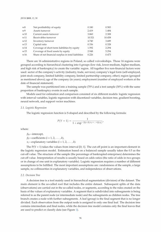
JRFM 2019, 12, 30
w8 Net profitability of equity 0.180 0.583w9 Assets turnover 2.419 1.484w10 Current assets turnover 3.860 2.308w11 Receivables turnover 10.521 10.458w12 Inventory turnover 4.740 3.689w13 Capital ratio 0.336 0.328w14 Coverage of short-term liabilities by equity 1.592 2.294w15 Coverage of fixed assets by equity 2.948 5.294w16 Share of net financial surplus in total liabilities 0.226 0.473
There are 16 administrative regions in Poland, so called voivodeships. Those 16 regions weregrouped according to hierarchical clustering into 4 groups (low risk, lower-medium, higher-medium,and high risk of bankruptcy) to create the variable: region. All together five non-financial factors wereused: sector of the company’s activity (industry, trade, services); company’s legal form (self-employed,joint stock company, limited liability company, limited partnership company, other); region (groupedas mentioned above); age of the company (in years); employment (number of employed workers at thedate of financial statement).
The sample was partitioned into a training sample (70%) and a test sample (30%) with the sameproportion of bankruptcy events in each sample.
Models used for estimation and comparison consisted of six different models: logistic regressionwith interval variables, logistic regression with discretized variables, decision tree, gradient boosting,neural network, and support vector machines.
2.1. Logistic Regression
The logistic regression function is S-shaped and described by the following formula:
P(Y = 1) =1
1 + exp−(β0+β1x1+...+βkxk),
where:
β0—intercept,βI—coefficients (i = 1, 2, . . . , k),xi—explanatory variables (i = 1, 2, . . . , k).
The P(Y = 1) takes the values from interval [0; 1]. The cut-off point is an important element inthe logistic regression model. Estimation based on a balanced sample usually takes the 0.5 as thecut-off value. The structure of the sample (the percentage of bankrupted enterprises) determines thecut-off value. Interpretation of results is usually based on odds ratios (the ratio of odds in two groupsor in change of one unit in explanatory variable). Logistic regression requires a number of differentassumptions to be fulfilled. The most important assumptions are: randomness of the sample, a largesample, no collinearities in explanatory variables, and independence of observations.
2.2. Decision Tree
A decision tree is a tool mainly used in hierarchical segmentation (division) of the dataset. Themain element is the so-called root that includes the entire dataset. Subsequent splits of the data(observations) are carried out in the so-called nodes, or segments, according to the rules created on thebasis of the values of explanatory variables. A segment that is subdivided into subsegments is beingreferred to as the parent node (or intermediate node) and the subsegments as children nodes. The treebranch creates a node with further subsegments. A leaf (group) is the final segment that is no longerdivided. Each observation from the output node is assigned to only one final leaf. The decision treecontains intermediate and final nodes, while the decision tree model contains only the final leaves thatare used to predict or classify data (see Figure 1).
96

JRFM 2019, 12, 30
Figure 1. Decision tree—graphical representation.
In order for decision trees to be used, a large collection of observations is required, as well assufficiently numerous cases for the dependent variable. Any (very) unusual observations may distortthe results, though this is not a major risk. A big risk in building the tree is overfitting, which can causeinstability of the model. The decision tree, unlikely the binary logistic regression, does not contain anyequations or coefficients, it is based only on the rules of dividing the dataset into separate groups. Asestimation of probabilities posteriori probabilities for each leaf are used. The rules generated by themodel from the learning set can be used for prediction (resulting in binary decisions).
The basic ways to measure the quality of the division for binary dependent variables or discretedependent variables with several categories include:
1. The degree of separation achieved by the division (measured by the Pearson chi-squared test),2. The degree of pollution reduction achieved by the division (measured by the reduction of entropy
or by the Gini coefficient).
The stopping criteria may be the following: the minimal number of observations in any final leaf,the critical size of any node, the number of splits in any path. After building a tree, it should be prunedinto an optimal size. The advantages of a decision tree are twofold: the results are easily interpretableand the model is flexible. Additionally, decision trees are not sensitive to missing data and do notrequire the normality of distributions or the equality of covariance matrices (as discriminant analysisdoes). The explanatory variables may differ in character, being either qualitative or quantitative.Decision trees automatically select important variables and may explain non-linear dependencies. Thedisadvantage of the decision trees is the fact that they can prove unstable and sensitive to the size ofthe training sample, validation or test sample results. The large size of the training sample is critical.Probabilities are approximated on the final leaf level. Overtraining is quite common in decision treesand the results for the training sample are usually much better than for the testing sample. All thosedisadvantages must be considered while building a model.
2.3. Gradient Boosting
Nowadays, a more popular method is the random forest, initially proposed by Breiman. It is amethod that takes together many classification trees. Firstly, we draw K bootstrap samples, then wecreate a classification tree for each of them in such a way that in each node we draw m (fewer thanthe number of all features) features which will participate in the selection of the best division. Treesare built without pruning. Finally, the observations are classified by the voting method. The onlyparameter of the method is the m coefficient, which should be much smaller than the dimension ofdata. The ease and speed with which random forests can be created makes them a feasible option evenfor very large data. Random forests are currently one of the most efficient classification methods, apart
97
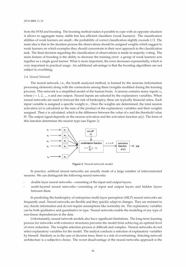
JRFM 2019, 12, 30
from the SVM and boosting. The boosting method makes it possible to cope with an opposite situation:it allows to aggregate many stable but less efficient classifiers (weak learners). The classificationabilities of weak learners are small—the probability of correct classification slightly exceeds 1/2. Themain idea is that in the iteration process the observations should be assigned weights which suggest toweak learners on which examples they should concentrate in their next approach to the classificationtask. The final decision regarding the classification of observations is made in majority voting. Themain feature of boosting is the ability to decrease the training error: a group of weak learners actstogether as a single good learner. What is more important, the error decreases exponentially, which isvery important in practical usage. An additional advantage is that the boosting algorithms are notsubject to overfitting.
2.4. Neural Network
The neural network, i.e., the fourth analyzed method, is formed by the neurons (informationprocessing elements) along with the connections among them (weights modified during the learningprocess). This network is a simplified model of the human brain. A neuron contains many inputs xi,where i = 1, 2, ..., n and one output. Neural inputs are selected by the explanatory variables. Whenneural networks are used to forecast the risk of bankruptcy, these are typically financial ratios. Eachinput variable is assigned a specific weight wi. Once the weights are determined, the total neuronactivation (e) is calculated as the sum of the product of the explanatory variables and their weightsassigned. Then y is calculated, which is the difference between the value of e and the threshold valueΘ. The output signal depends on the neuron activation and the activation function ϕ(y). The form ofthis function determines the neuron type (see Figure 2).
Figure 2. Neural network model.
In practice, artificial neural networks are usually made of a large number of interconnectedneurons. We can distinguish the following neural networks:
- double layer neural networks—consisting of the input and output layers;- multi-layered neural networks—consisting of input and output layers and hidden layers
between them.
In predicting the bankruptcy of enterprises multi-layer perceptron (MLP) neural networks arefrequently used. Neural networks are flexible and they quickly adapt to changes. They are resistant toany chaotic information and do not require assumptions like normality etc. The explanatory variablescan be both qualitative and quantitative in type. Neural networks enable the modeling of any type ofnon-linear dependencies in the data.
Unfortunately, neural network models also have significant limitations. The long-term learningprocess for networks with extensive structures prevents the model from achieving an optimal levelof error reduction. The weights selection process is difficult and complex. Neural networks do notselect explanatory variables for the model. The analyst conducts a selection of explanatory variablesby himself. Similarly as in the case of decision trees, there is a risk of overtraining. Selecting networkarchitecture is a subjective choice. The worst disadvantage of the neural networks approach is the
98
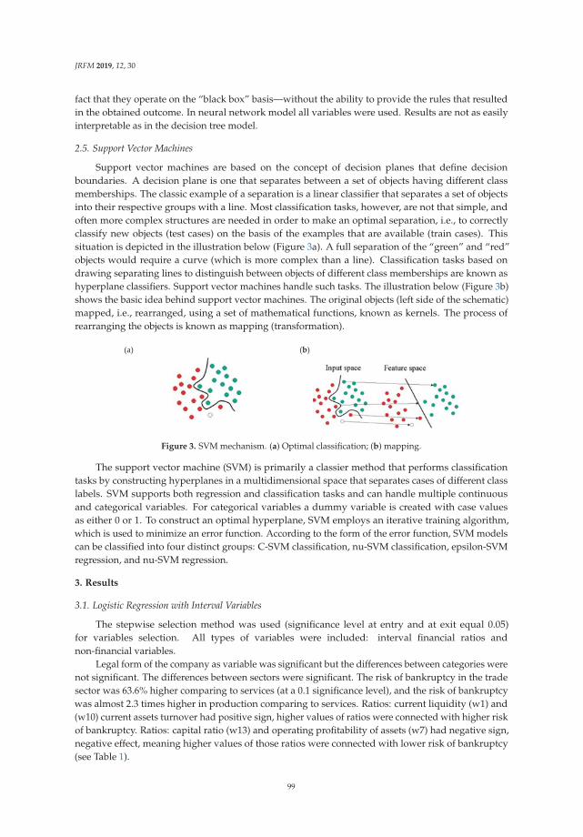
JRFM 2019, 12, 30
fact that they operate on the “black box” basis—without the ability to provide the rules that resultedin the obtained outcome. In neural network model all variables were used. Results are not as easilyinterpretable as in the decision tree model.
2.5. Support Vector Machines
Support vector machines are based on the concept of decision planes that define decisionboundaries. A decision plane is one that separates between a set of objects having different classmemberships. The classic example of a separation is a linear classifier that separates a set of objectsinto their respective groups with a line. Most classification tasks, however, are not that simple, andoften more complex structures are needed in order to make an optimal separation, i.e., to correctlyclassify new objects (test cases) on the basis of the examples that are available (train cases). Thissituation is depicted in the illustration below (Figure 3a). A full separation of the “green” and “red”objects would require a curve (which is more complex than a line). Classification tasks based ondrawing separating lines to distinguish between objects of different class memberships are known ashyperplane classifiers. Support vector machines handle such tasks. The illustration below (Figure 3b)shows the basic idea behind support vector machines. The original objects (left side of the schematic)mapped, i.e., rearranged, using a set of mathematical functions, known as kernels. The process ofrearranging the objects is known as mapping (transformation).
(a)
(b)
Figure 3. SVM mechanism. (a) Optimal classification; (b) mapping.
The support vector machine (SVM) is primarily a classier method that performs classificationtasks by constructing hyperplanes in a multidimensional space that separates cases of different classlabels. SVM supports both regression and classification tasks and can handle multiple continuousand categorical variables. For categorical variables a dummy variable is created with case valuesas either 0 or 1. To construct an optimal hyperplane, SVM employs an iterative training algorithm,which is used to minimize an error function. According to the form of the error function, SVM modelscan be classified into four distinct groups: C-SVM classification, nu-SVM classification, epsilon-SVMregression, and nu-SVM regression.
3. Results
3.1. Logistic Regression with Interval Variables
The stepwise selection method was used (significance level at entry and at exit equal 0.05)for variables selection. All types of variables were included: interval financial ratios andnon-financial variables.
Legal form of the company as variable was significant but the differences between categories werenot significant. The differences between sectors were significant. The risk of bankruptcy in the tradesector was 63.6% higher comparing to services (at a 0.1 significance level), and the risk of bankruptcywas almost 2.3 times higher in production comparing to services. Ratios: current liquidity (w1) and(w10) current assets turnover had positive sign, higher values of ratios were connected with higher riskof bankruptcy. Ratios: capital ratio (w13) and operating profitability of assets (w7) had negative sign,negative effect, meaning higher values of those ratios were connected with lower risk of bankruptcy(see Table 1).
99
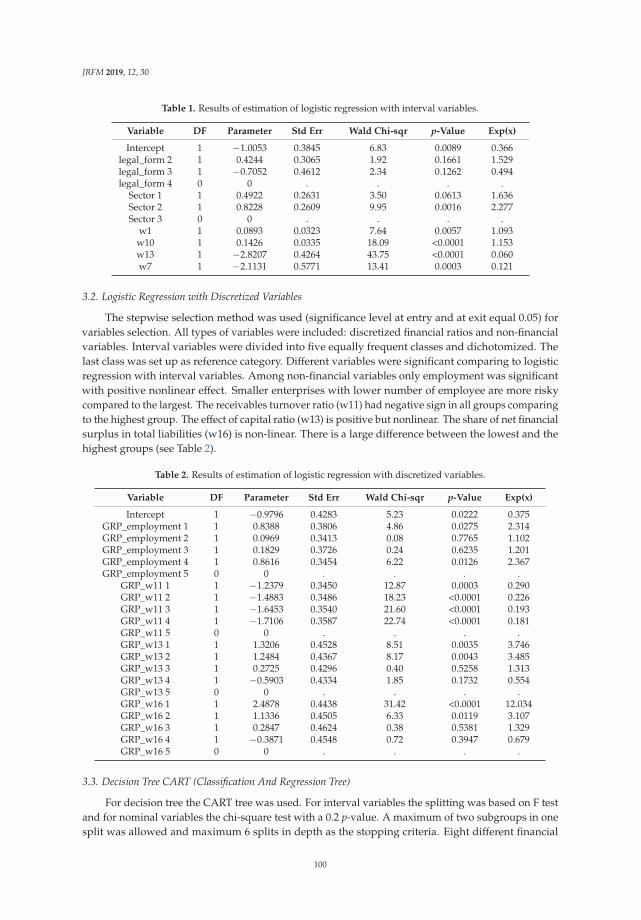
JRFM 2019, 12, 30
Table 1. Results of estimation of logistic regression with interval variables.
Variable DF Parameter Std Err Wald Chi-sqr p-Value Exp(x)
Intercept 1 −1.0053 0.3845 6.83 0.0089 0.366legal_form 2 1 0.4244 0.3065 1.92 0.1661 1.529legal_form 3 1 −0.7052 0.4612 2.34 0.1262 0.494legal_form 4 0 0 . . . .
Sector 1 1 0.4922 0.2631 3.50 0.0613 1.636Sector 2 1 0.8228 0.2609 9.95 0.0016 2.277Sector 3 0 0 . . . .
w1 1 0.0893 0.0323 7.64 0.0057 1.093w10 1 0.1426 0.0335 18.09 <0.0001 1.153w13 1 −2.8207 0.4264 43.75 <0.0001 0.060w7 1 −2.1131 0.5771 13.41 0.0003 0.121
3.2. Logistic Regression with Discretized Variables
The stepwise selection method was used (significance level at entry and at exit equal 0.05) forvariables selection. All types of variables were included: discretized financial ratios and non-financialvariables. Interval variables were divided into five equally frequent classes and dichotomized. Thelast class was set up as reference category. Different variables were significant comparing to logisticregression with interval variables. Among non-financial variables only employment was significantwith positive nonlinear effect. Smaller enterprises with lower number of employee are more riskycompared to the largest. The receivables turnover ratio (w11) had negative sign in all groups comparingto the highest group. The effect of capital ratio (w13) is positive but nonlinear. The share of net financialsurplus in total liabilities (w16) is non-linear. There is a large difference between the lowest and thehighest groups (see Table 2).
Table 2. Results of estimation of logistic regression with discretized variables.
Variable DF Parameter Std Err Wald Chi-sqr p-Value Exp(x)
Intercept 1 −0.9796 0.4283 5.23 0.0222 0.375GRP_employment 1 1 0.8388 0.3806 4.86 0.0275 2.314GRP_employment 2 1 0.0969 0.3413 0.08 0.7765 1.102GRP_employment 3 1 0.1829 0.3726 0.24 0.6235 1.201GRP_employment 4 1 0.8616 0.3454 6.22 0.0126 2.367GRP_employment 5 0 0 . . . .
GRP_w11 1 1 −1.2379 0.3450 12.87 0.0003 0.290GRP_w11 2 1 −1.4883 0.3486 18.23 <0.0001 0.226GRP_w11 3 1 −1.6453 0.3540 21.60 <0.0001 0.193GRP_w11 4 1 −1.7106 0.3587 22.74 <0.0001 0.181GRP_w11 5 0 0 . . . .GRP_w13 1 1 1.3206 0.4528 8.51 0.0035 3.746GRP_w13 2 1 1.2484 0.4367 8.17 0.0043 3.485GRP_w13 3 1 0.2725 0.4296 0.40 0.5258 1.313GRP_w13 4 1 −0.5903 0.4334 1.85 0.1732 0.554GRP_w13 5 0 0 . . . .GRP_w16 1 1 2.4878 0.4438 31.42 <0.0001 12.034GRP_w16 2 1 1.1336 0.4505 6.33 0.0119 3.107GRP_w16 3 1 0.2847 0.4624 0.38 0.5381 1.329GRP_w16 4 1 −0.3871 0.4548 0.72 0.3947 0.679GRP_w16 5 0 0 . . . .
3.3. Decision Tree CART (Classification And Regression Tree)
For decision tree the CART tree was used. For interval variables the splitting was based on F testand for nominal variables the chi-square test with a 0.2 p-value. A maximum of two subgroups in onesplit was allowed and maximum 6 splits in depth as the stopping criteria. Eight different financial
100
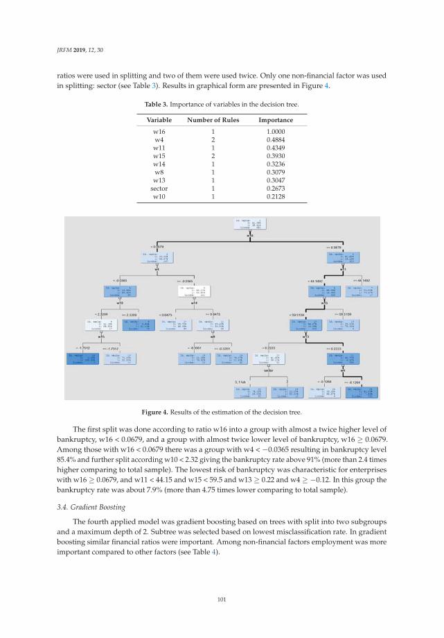
JRFM 2019, 12, 30
ratios were used in splitting and two of them were used twice. Only one non-financial factor was usedin splitting: sector (see Table 3). Results in graphical form are presented in Figure 4.
Table 3. Importance of variables in the decision tree.
Variable Number of Rules Importance
w16 1 1.0000w4 2 0.4884
w11 1 0.4349w15 2 0.3930w14 1 0.3236w8 1 0.3079
w13 1 0.3047sector 1 0.2673w10 1 0.2128
Figure 4. Results of the estimation of the decision tree.
The first split was done according to ratio w16 into a group with almost a twice higher level ofbankruptcy, w16 < 0.0679, and a group with almost twice lower level of bankruptcy, w16 ≥ 0.0679.Among those with w16 < 0.0679 there was a group with w4 < −0.0365 resulting in bankruptcy level85.4% and further split according w10 < 2.32 giving the bankruptcy rate above 91% (more than 2.4 timeshigher comparing to total sample). The lowest risk of bankruptcy was characteristic for enterpriseswith w16 ≥ 0.0679, and w11 < 44.15 and w15 < 59.5 and w13 ≥ 0.22 and w4 ≥ −0.12. In this group thebankruptcy rate was about 7.9% (more than 4.75 times lower comparing to total sample).
3.4. Gradient Boosting
The fourth applied model was gradient boosting based on trees with split into two subgroupsand a maximum depth of 2. Subtree was selected based on lowest misclassification rate. In gradientboosting similar financial ratios were important. Among non-financial factors employment was moreimportant compared to other factors (see Table 4).
101
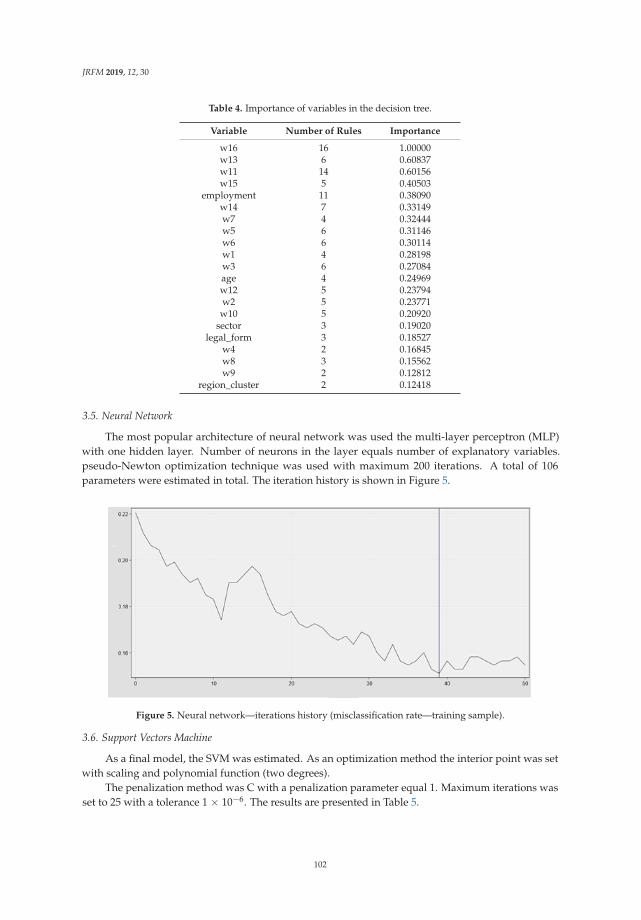
JRFM 2019, 12, 30
Table 4. Importance of variables in the decision tree.
Variable Number of Rules Importance
w16 16 1.00000w13 6 0.60837w11 14 0.60156w15 5 0.40503
employment 11 0.38090w14 7 0.33149w7 4 0.32444w5 6 0.31146w6 6 0.30114w1 4 0.28198w3 6 0.27084age 4 0.24969w12 5 0.23794w2 5 0.23771w10 5 0.20920
sector 3 0.19020legal_form 3 0.18527
w4 2 0.16845w8 3 0.15562w9 2 0.12812
region_cluster 2 0.12418
3.5. Neural Network
The most popular architecture of neural network was used the multi-layer perceptron (MLP)with one hidden layer. Number of neurons in the layer equals number of explanatory variables.pseudo-Newton optimization technique was used with maximum 200 iterations. A total of 106parameters were estimated in total. The iteration history is shown in Figure 5.
Figure 5. Neural network—iterations history (misclassification rate—training sample).
3.6. Support Vectors Machine
As a final model, the SVM was estimated. As an optimization method the interior point was setwith scaling and polynomial function (two degrees).
The penalization method was C with a penalization parameter equal 1. Maximum iterations wasset to 25 with a tolerance 1 × 10⁻⁶. The results are presented in Table 5.
102

JRFM 2019, 12, 30
Table 5. Results of SVM training.
Internal product of weights 46.3039131Burden –21.744579Total stock (violation of restrictions) 305.767624Norm of the longest vector 11.6448785Number of support vectors 387Number of support vectors on margin 334Maximal F 2.84554647Minimal F –21.760742Number of effects 21Columns of data matrix 36Columns of kernel matrix 703
3.7. Model Comparison
Model evaluation was based on the Gini (accuracy ratio—AR) coefficient on the test sample,which is a measure based on ROC, i.e., the curve used to measure the discriminative power of themodel. It is applied in the case when the dependent variable is binary (it has two unique values).The Figure 6 presents the relation of the specificity to the sensitivity of the model. Both of thosemeasures provide information on how effective the classification is in the context of both levels of thedependent variable. The ROC curve is a sensitivity function (on the vertical axis) and 1-specificity (onthe horizontal axis). Each point of the curve corresponds to a given point of split (section). Points in theright upper corner correspond to a low q level. Points in the left bottom corner relate to a high q level.ROC does not depend on the assumed point of split. The rates are drawn for all points of split. Whileselecting a given point of split we can establish the specificity and sensitivity of the model for thatpoint. Selecting a given point of split we can establish the number of successes and failures predictedby the model, and then calculate the sensitivity and the specificity of the model. The correspondentsensitivity and specificity levels are easy to read from the graph of the ROC curve. A good model hasthe ROC curve close to the upper-left boundary of the graph. Then we can find points on the curverepresenting high values both in terms of sensitivity and specificity (e.g., so that c > 0.8 and s > 0.8).The random model has the ROC curve lying on the diagonal. Then the sensitivity + specificity = 1for all the threshold values of q. In such a case while establishing the value c > 0.8 we cannot ensurethat the specificity is greater than 0.2. The ROC curve is helpful when selecting the optimal point ofdivision. For example, we choose the threshold that gives equal probability of misclassification in eachclass. We also have to take into account the different cost of both types of misclassification and decidewhether to provide high sensitivity or high specificity. The area under the ROC curve is a measure ofthe quality of the model. This way we can compare the quality of different models. The AUC (areaunder the ROC curve) for an ideal model equals 1 and for a random model 0.5.
The similar measure to ROC is the CAP curve, where the cumulative frequencies for goodcustomers are substituted by frequencies for all customers. The area under the CAP curve is called theaccuracy ratio. The CAP curve represents the y% of bankrupted enterprises that can be found in thex% of the worst assessed enterprises within the model. The curve should be concave. The accuracyratio (Gini coefficient) based on the CAP curve is defined as:
AR =
1∫0
f (x)dx − 12
12 − 1
2 BR, (1)
where:
BR—bankruptcy rate;1∫
0f (x)dx − 1
2 —area under the CAP curve.
103
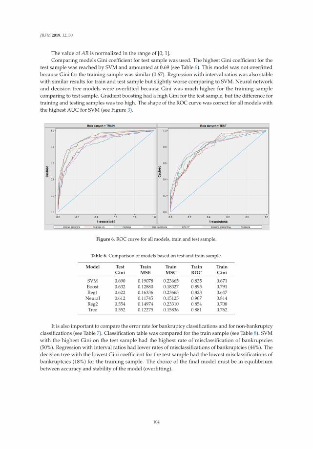
JRFM 2019, 12, 30
The value of AR is normalized in the range of [0; 1].Comparing models Gini coefficient for test sample was used. The highest Gini coefficient for the
test sample was reached by SVM and amounted at 0.69 (see Table 6). This model was not overfittedbecause Gini for the training sample was similar (0.67). Regression with interval ratios was also stablewith similar results for train and test sample but slightly worse comparing to SVM. Neural networkand decision tree models were overfitted because Gini was much higher for the training samplecomparing to test sample. Gradient boosting had a high Gini for the test sample, but the difference fortraining and testing samples was too high. The shape of the ROC curve was correct for all models withthe highest AUC for SVM (see Figure 3).
Figure 6. ROC curve for all models, train and test sample.
Table 6. Comparison of models based on test and train sample.
Model Test Train Train Train TrainGini MSE MSC ROC Gini
SVM 0.690 0.19078 0.23665 0.835 0.671Boost 0.632 0.12880 0.18327 0.895 0.791Reg1 0.622 0.16336 0.23665 0.823 0.647
Neural 0.612 0.11745 0.15125 0.907 0.814Reg2 0.554 0.14974 0.23310 0.854 0.708Tree 0.552 0.12275 0.15836 0.881 0.762
It is also important to compare the error rate for bankruptcy classifications and for non-bankruptcyclassifications (see Table 7). Classification table was compared for the train sample (see Table 8). SVMwith the highest Gini on the test sample had the highest rate of misclassification of bankruptcies(50%). Regression with interval ratios had lower rates of misclassifications of bankruptcies (44%). Thedecision tree with the lowest Gini coefficient for the test sample had the lowest misclassifications ofbankruptcies (18%) for the training sample. The choice of the final model must be in equilibriumbetween accuracy and stability of the model (overfitting).
104
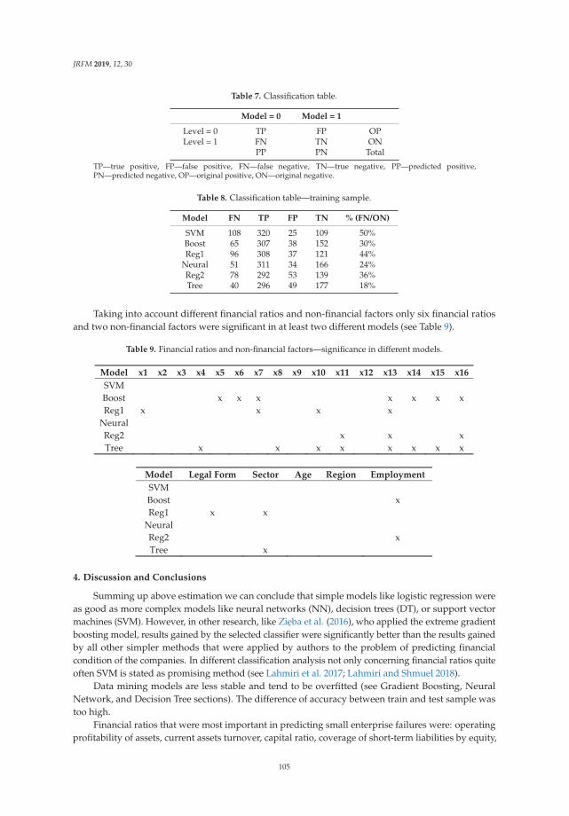
JRFM 2019, 12, 30
Table 7. Classification table.
Model = 0 Model = 1
Level = 0 TP FP OPLevel = 1 FN TN ON
PP PN Total
TP—true positive, FP—false positive, FN—false negative, TN—true negative, PP—predicted positive,PN—predicted negative, OP—original positive, ON—original negative.
Table 8. Classification table—training sample.
Model FN TP FP TN % (FN/ON)
SVM 108 320 25 109 50%Boost 65 307 38 152 30%Reg1 96 308 37 121 44%
Neural 51 311 34 166 24%Reg2 78 292 53 139 36%Tree 40 296 49 177 18%
Taking into account different financial ratios and non-financial factors only six financial ratiosand two non-financial factors were significant in at least two different models (see Table 9).
Table 9. Financial ratios and non-financial factors—significance in different models.
Model x1 x2 x3 x4 x5 x6 x7 x8 x9 x10 x11 x12 x13 x14 x15 x16 SVM Boost x x x x x x x Reg1 x x x x
Neural Reg2 x x x Tree x x x x x x x x
Model Legal Form Sector Age Region Employment SVM Boost x Reg1 x x
Neural Reg2 x Tree x
4. Discussion and Conclusions
Summing up above estimation we can conclude that simple models like logistic regression wereas good as more complex models like neural networks (NN), decision trees (DT), or support vectormachines (SVM). However, in other research, like Zieba et al. (2016), who applied the extreme gradientboosting model, results gained by the selected classifier were significantly better than the results gainedby all other simpler methods that were applied by authors to the problem of predicting financialcondition of the companies. In different classification analysis not only concerning financial ratios quiteoften SVM is stated as promising method (see Lahmiri et al. 2017; Lahmiri and Shmuel 2018).
Data mining models are less stable and tend to be overfitted (see Gradient Boosting, NeuralNetwork, and Decision Tree sections). The difference of accuracy between train and test sample wastoo high.
Financial ratios that were most important in predicting small enterprise failures were: operatingprofitability of assets, current assets turnover, capital ratio, coverage of short-term liabilities by equity,
105

JRFM 2019, 12, 30
coverage of fixed assets by equity, and share of net financial surplus in total liabilities. Results may becompared to results recently obtained for Polish bankruptcy data by Zieba et al. (2016). The authorsexamined data for Polish bankrupted companies from period 2007–2013. They analyzed a five-yearperiod and only three indicators: adjusted share of equity in financing of assets, current ratio, liabilitiesturnover ratio appeared in each analyzed year. According to authors those ratios can be considered asuseful in predicting bankruptcy of enterprises.
Among non-financial factors two of them were important: sector of activity and employment.The usage of non-financial ratios improves the results of all models which confirmed our expectationsand other research. The legal form of the company seems to be the most important variable among allthe considered non-financial factors. Employment and sector also plays a role, which confirms theresults obtained by Chava and Jarrow (2004). Gordini (2014) confirmed that building models tailoredto specific geographical areas increases the accuracy. However, in our models two variables, regionand age of the company, seem to play a much less important role.
The hypotheses were positively verified:
Hypothesis 3 (H3): Non-financial factors are important in case of predicting small enterprises successand failures.
Hypothesis 4 (H4): More advanced and complicated models are not necessary to predict small enterprisefailures. Simple models are as effective as more complex ones.
As always the greatest problem is the access to good quality data. Depending on the dataavailability future research would cover the interaction with the macroeconomic situation. Financialsituations expanded by non-financial factors do not give the full view of the bankruptcy causes. Deeperanalysis of causality mechanisms is needed.
Funding: This research received no external funding.
Conflicts of Interest: The authors declare no conflict of interest.
References
Altman, Edward I. 1968. Financial ratios, Discriminant analysis and the prediction of corporate bankruptcy.Journal of Finance 23: 589–609. [CrossRef]
Appenzeller, Dorota, and Katarzyna Szarzec. 2004. Forecasting the bankruptcy risk of Polish public companies.Rynek Terminowy 1: 120–28.
Aziz, M. Adnan, and Humayon A. Dar. 2006. Predicting Corporate Bankruptcy: Where do We Stand? CorporateGovernance International Journal of Business in Society 6: 18–33. [CrossRef]
Back, Barbro, Teija Laitinen, Kaisa Sere, and Michiel van Wezel. 1996. Choosing Bankruptcy Predictors UsingDiscriminant Analysis, Logit Analysis, and Genetic Algorithms. Technical Report. Turku: Turku Centre forComputer Science.
Balina, Rafał, and Maksymilian Jan Bak. 2016. Discriminant Analysis as a Prediction Method for Corporate Bankruptcywith the Industrial Aspects. Walenczów: Wydawnictwo Naukowe Intellect.
Blanco-Oliver, Antonio, Rafael Pino-Mejías, Juan Lara-Rubio, and Salvador Rayo. 2013. Credit scoring models forthe microfinance industry using neural networks: Evidence from Peru. Expert Systems with Applications 40:356–64. [CrossRef]
Brozyna, Jacek, Grzegorz Mentel, and Tomasz Pisula. 2016. Statistical methods of the bankruptcy prediction in thelogistics sector in Poland and Slovakia. Transformations in Business & Economics 15: 80–96.
Calabrese, Raffaella, Giampiero Marra, and Silvia Angela Osmetti. 2015. Bankruptcy prediction of small andmedium enterprises using a flexible binary generalized extreme value model. Journal of the OperationalResearch Society 67: 604–15. [CrossRef]
Chaudhuri, Arindam, and Kajal De. 2011. Fuzzy support vector machine for bankruptcy prediction. Applied SoftComputing 11: 2472–86. [CrossRef]
106

JRFM 2019, 12, 30
Chava, Sudheer, and Robert A. Jarrow. 2004. Bankruptcy prediction with industry effects. Review of Finance 8:537–569. [CrossRef]
Gajdka, Jerzy, and Daniel Stos. 1996. The use of discriminant analysis in assessing the financial conditionof enterprises. In Restructuring in the Process of Transformation and Development of Enterprises. Edited byRyszard Borowiecki. Kraków: Wydawnictwo Akademii Ekonomicznej w Krakowie.
Gaska, Damian. 2016. Predicting Bankruptcy of Enterprises with the use of Learning Methods. Ph.D. dissertation,Wrocław University of Economics, Wrocław, Poland.
Gordini, Niccolo. 2014. A genetic algorithm approach for SMEs bankruptcy prediction: Empirical evidence fromItaly. Expert Systems with Applications 41: 6067–536. [CrossRef]
Gruszczynski, Marek. 2003. Models of Microeconometrics in the Analysis and Forecasting of the Financial Risk ofEnterprises. Warszawa: Zeszyty Polskiej Akademii Nauk nr 23.
Gupta, Jairaj, Andros Gregoriou, and Jerome Healy. 2015. Forecasting bankruptcy for SMEs using hazard function: Areview of quantitative finance and accounting. Review of Quantitative Finance and Accounting 45: 845–69. [CrossRef]
Hadasik, Dorota. 1998. The Bankruptcy of Enterprises in Poland and Methods of its Forecasting. Poznan: WydawnictwoAkademii Ekonomicznej w Poznaniu, vol. 153.
Hamrol, Mirosław, Bartłomiej Czajka, and Maciej Piechocki. 2004. Enterprise bankruptcy—discriminant analysismodel. Przeglad Organizacji 6: 35–39.
Hołda, Artur. 2001. Forecasting the bankruptcy of an enterprise in the conditions of the Polish economy using thediscriminatory function ZH. Rachunkowosc 5: 306–10.
Jagiełło, Robert. 2013. Discriminant and Logistic Analysis in the Process of Assessing the Creditworthiness of Enterprises.Materiały i Studia, Zeszyt 286. Warszawa: NBP.
Jiménez, Gabriel, and Jesus Saurina. 2004. Collateral, type of lender and relationship banking as determinants ofcredit risk. Journal of Banking & Finance 28: 2191–212.
Kalak, El Izidin, and Robert Hudson. 2016. The effect of size on the failure probabilities of SMEs: An empiricalstudy on the US market using discrete hazard model. International Review of Financial Analysis 43: 135–45.[CrossRef]
Karbownik, Lidia. 2017. Methods for Assessing the Financial Risk of Enterprises in the TSI Sector in Poland. Łódz:Wydawnictwo Uniwersytetu Łódzkiego.
Kim, Hong Sik, and So Young Sohn. 2010. Support Vector Machines for Default Prediction of SMEs Based onTechnology Credit. European Journal of Operational Research 201: 838–46. [CrossRef]
Korol, Tomasz. 2004. Assessment of the Accuracy of the Application of Discriminatory Methods and ArtificialNeural Networks for the Identification of Enterprises Threatened with Bankruptcy. Doctoral dissertation,University of Gdansk, Gdansk, Poland.
Korol, Tomasz. 2010a. Early Warning Systems of Enterprises to the Risk of Bankruptcy. Warszawa: Wolters Kluwer.Korol, Tomasz. 2010b. Forecasting bankruptcies of companies using soft computing techniques. Finansowy
Kwartalnik Internetowy “e-Finanse” 6: 1–14.Lahmiri, Salim. 2016a. Features selection, data mining and financial risk classification: A comparative study.
Intelligent Systems in Accounting. Finance and Management 23: 265–75.Lahmiri, Salim. 2016b. On simulation performance of feedforward and NARX networks under different numerical
training algorithms. In Handbook of Research on Computational Simulation and Modeling in Engineering. Hershey: IGI.Lahmiri, Salim. 2016c. Prediction of International Stock Markets Based on Hybrid Intelligent Systems. In Handbook
of Research on Innovations in Information Retrieval, Analysis, and Management. Hershey: IGI.Lahmiri, Salim. 2017. A two-step system for direct bank telemarketing outcome classification. Intelligent Systems
in Accounting. Finance and Management 24: 49–55.Lahmiri, Salim, Debra Ann Dawson, and Amir Smuel. 2017. Performance of machine learning methods in
diagnosing Parkinson’s disease based on dysphonia measures. Biomedical Engineering Letters 8: 1–11.[CrossRef] [PubMed]
Lahmiri, Salim, and Amir Shmuel. 2018. Performance of machine learning methods applied to structural MRIand ADAS cognitive scores in diagnosing Alzheimer’s disease. Biomedical Signal Processing and Control.[CrossRef]
Maczynska, Elzbieta. 1994. Assessment of the condition of the enterprise. Simplified methods. Zycie Gospodarcze38: 42–45.
Maczynska, Elzbieta. 2004. Early warning systems. Nowe Zycie Gospodarcze 12: 4–9.
107

JRFM 2019, 12, 30
Michaluk, Krzysztof. 2003. Effectiveness of corporate bankruptcy models in Polish economic conditions. InCorporate Finance in the Face of Globalization Processes. Edited by Leszek Pawłowicz and Ryszard Wierzba.Warszawa: Wydawnictwo Gdanskiej Akademii Bankowej.
Ong, Chorng-Shyong, Jih-Jeng Huang, and Gwo-Hshiung Tzeng. 2005. Building credit scoring models usinggenetic programming. Expert Systems with Applications 29: 41–47. [CrossRef]
Pociecha, Józef, and Barbara Pawełek. 2011. Bankruptcy Prediction and Business Cycle, ContemporaryProblems of Transformation Process in the Central and East European Countries. Paper presented at17th Ukrainian-Polish-Slovak Scientific Seminar, Lviv, Ukraine, September 22–24; Lviv: The Lviv Academyof Commerce, pp. 9–24.
Pociecha, Józef, Barbara Pawełek, Mateusz Baryła, and Sabina Augustyn. 2014. Statistical Methods of ForecastingBankruptcy in the Changing Economic Situation. Kraków: Fundacja Uniwersytetu Ekonomicznego w Krakowie.
Pogodzinska, Marzanna, and Sławomir Sojak. 1995. The Use of Discriminant Analysis in Predicting Bankruptcy ofEnterprises. Ekonomia XXV, Zeszyt 299. Torun: AUNC.
Prusak, Błazej. 2018. Review of Research into Enterprise Bankruptcy Prediction in Selected Central and EasternEuropean Countries. International Journal of Financial Studies 6: 60. [CrossRef]
Prusak, Błazej, and Agnieszka Wieckowska. 2007. Multidimensional models of discriminant analysis in the studyof the bankruptcy risk of Polish companies listed on the WSE. In Economic and Legal Aspects of CorporateBankruptcy. Edited by Błazej Prusak. Warszawa: Difin.
Prusak, Błazej. 2005. Modern Methods of Forecasting Financial Risk of Enterprises. Warszawa: Difin.Psillaki, Maria, Ioannis E. Tsolas, and Dimitris Margaritis. 2010. Evaluation of credit risk based on firm
performance. European Journal of Operational Research 201: 873–81. [CrossRef]Ptak-Chmielewska, Aneta, and Anna Matuszyk. 2017. The importance of financial and non-financial ratios in
SMEs bankruptcy prediction. Bank i Kredyt 49: 45–62.Ptak-Chmielewska, Aneta. 2016. Statistical Models for Corporate Credit Risk Assessment—Rating Models. Acta
Universitatis Lodziensis Folia Oeconomica 3: 98–111. [CrossRef]Sartori, Fabio, Alice Mazzucchelli, and Angelo Di Gregorio. 2016. Bankruptcy forecasting using case-based
reasoning: The CRePERIE approach. Expert Systems with Applications 64: 400–11. [CrossRef]Sohn, So Young, Dong Ha Kim, and Jin Hee Yoon. 2016. Technology credit scoring model with fuzzy logistic
regression. Applied Soft Computing 43: 150–58. [CrossRef]Sojak, Sławomir, and Józef Stawicki. 2000. The use of taxonomic methods to assess the economic condition of
enterprises. Zeszyty Teoretyczne Rachunkowosci 3: 55–66.Stepien, Paweł, and Tomasz Strak. 2003. Signs of the threat of bankruptcy of Polish enterprises—Empirical study.
In Time for Money, t. II. Edited by Dariusz Zarzecki. Szczecin: Wydawnictwo Uniwersytetu Szczecinskiego.Stepien, Paweł, and Tomasz Strak. 2004. Multidimensional logit models for assessing the risk of bankruptcy of
Polish enterprises. In Time for Money, t. I. Edited by Dariusz Zarzecki. Szczecin: Wydawnictwo UniwersytetuSzczecinskiego.
Wedzki, Dariusz. 2000. The problem of using the ratio analysis to predict the bankruptcy of Polishenterprises—Case study. Bank i Kredyt 5: 54–61.
Wedzki, Dariusz. 2004. Logit model of bankruptcy for the Polish economy—Conclusions from the study. InTime for Money. Corporate Finance. Financing Enterprises in the EU. Edited by Dariusz Zarzecki. Szczecin:Wydawnictwo Uniwersytetu Szczecinskiego.
Wierzba, Dariusz. 2000. Early Detection of Enterprises Threatened with Bankruptcy Based on the Analysis of FinancialRatios—Theory and Empirical Research. Zeszyty Naukowe nr 9. Warszawa: Wydawnictwo Wyzszej SzkołyEkonomiczno-Informatycznej w Warszawie.
Zieba, Maciej, Sebastian K. Tomczak, and Jakub M. Tomczak. 2016. Ensemble boosted trees with synthetic featuresgeneration in application to bankruptcy prediction. Expert Systems with Applications 58: 93–101. [CrossRef]
Zmijewski, Me. 1984. Methodological issues related to the estimation of financial distress prediction models.Journal of Accounting Research 22: 59–82. [CrossRef]
© 2019 by the author. Licensee MDPI, Basel, Switzerland. This article is an open accessarticle distributed under the terms and conditions of the Creative Commons Attribution(CC BY) license (http://creativecommons.org/licenses/by/4.0/).
108
Journal of
Risk and FinancialManagement
Article
Ensemble Learning or Deep Learning? Application toDefault Risk Analysis
Shigeyuki Hamori 1,* ID , Minami Kawai 2, Takahiro Kume 2, Yuji Murakami 2
and Chikara Watanabe 2
1 Graduate School of Economics, Kobe University, Kobe 657-8501, Japan2 Department of Economics, Kobe University, Kobe 657-8501, Japan; [email protected] (M.K.);
[email protected] (T.K.); [email protected] (Y.M.); [email protected] (C.W.)* Correspondence; [email protected]; Tel.: +81-78-803-6832
Received: 19 January 2018; Accepted: 28 February 2018; Published: 5 March 2018
Abstract: Proper credit-risk management is essential for lending institutions, as substantial losses canbe incurred when borrowers default. Consequently, statistical methods that can measure and analyzecredit risk objectively are becoming increasingly important. This study analyzes default paymentdata and compares the prediction accuracy and classification ability of three ensemble-learningmethods—specifically, bagging, random forest, and boosting—with those of various neural-networkmethods, each of which has a different activation function. The results obtained indicate that theclassification ability of boosting is superior to other machine-learning methods including neuralnetworks. It is also found that the performance of neural-network models depends on the choice ofactivation function, the number of middle layers, and the inclusion of dropout.
Keywords: credit risk; ensemble learning; deep learning; bagging; random forest; boosting; deepneural network
1. Introduction
Credit-risk management is essential for financial institutions whose core business is lending.Thus, accurate consumer or corporation credit assessment is of utmost importance because significantlosses can be incurred by financial institutions when borrowers default. To control their losses fromuncollectable accounts, financial institutions therefore need to properly assess borrowers’ credit risks.Consequently, they endeavor to collate borrower data, and various statistical methods have beendeveloped to measure and analyze credit risk objectively.
Because of its academic and practical importance, much research has been conducted on thisissue. For example, Boguslauskas and Mileris (2009) analyzed credit risk using Lithuanian data for50 cases of successful enterprises and 50 cases of bankrupted enterprises. Their results indicated thatartificial neural networks are an efficient method to estimate the credit risk.
Angelini, Tollo, and Roli (Angelini et al. 2008) presented the application of an artificial neuralnetwork for credit-risk assessment using the data of 76 small businesses from a bank in Italy. Theyused two neural architectures to classify borrowers into two distinct classes: in bonis and default.One is a feedforward neural network and is composed of an input layer, two hidden layers and anoutput layer. The other is a four-layer feedforward neural network with ad hoc connections and inputneurons grouped in sets of three. Their results indicate that neural networks successfully identify thein bonis/default tendency of a borrower.
Khshman (2009) developed a system of credit-risk evaluation using a neural network and appliedthe system to Australian credit data (690 cases; 307 creditworthy instances and 383 non-creditworthyinstances). He compared the performance of the single-hidden layer neural network (SHNN) modeland double-hidden layer network (DHNN). His experimental results indicated that the system with
JRFM 2018, 11, 12; doi:10.3390/jrfm11010012 www.mdpi.com/journal/jrfm109

JRFM 2018, 11, 12
SHNN outperformed the system with DHNN for credit-risk evaluation, and thus the SHNN neuralsystem was recommended for the automatic processing of credit applications.
Yeh and Lien (2009) compared the predictive accuracy of probability of default amongsix data-mining methods (specifically, K-nearest neighbor classifier, logistic regression, discriminantanalysis, naive Bayesian classifier, artificial neural networks, and classification trees) using customers’default payments data in Taiwan. Their experimental results indicated that only artificial neuralnetworks can accurately estimate default probability.
Khashman (2010) employed neural-network models for credit-risk evaluation with Germancredit data comprising 1000 cases: 700 instances of creditworthy applicants and 300 instances whereapplicants were not creditworthy.1 The results obtained indicated that the accuracy rates for thetraining data and test data were 99.25% and 73.17%, respectively. In this data, however, if onealways predicts that a case is creditworthy, then the accuracy rate naturally converges to 70%. Thus,the results imply that there is only a 3.17% gain for the prediction accuracy of test data using neuralnetwork models.
Gante et al. (2015) also used German credit data and compared 12 neural-network models to assesscredit risk. Their results indicated that a neural network with 20 input neurons, 10 hidden neurons,and one output neuron is a suitable neural network model for use in a credit risk evaluation system.
Khemakhem and Boujelbene (2015) compared the prediction of a neural network with that ofdiscriminant analysis using 86 Tunisian client companies of a Tunisian commercial bank over threeyears. Their results indicated that a neural network outperforms discriminant analysis in predictingcredit risk.
As is pointed out by Oreski et al. (2012), the majority of studies have shown that neural networksare more accurate, flexible and robust than conventional statistical methods for the assessment ofcredit risk.
In this study, we use 11 machine-learning methods to predict the default risk based on clients’attributes, and compare their prediction accuracy. Specifically, we employ three ensemble learningmethods—bagging, random forest, and boosting—and eight neural network methods with differentactivation functions. The performance of each method is compared in terms of their ability to predictthe default risk using multiple indicators (accuracy, rate of prediction, results, receiver operatingcharacteristic (ROC) curve, area under the curve (AUC), and F-score).2
The results obtained indicate that the classification ability of boosting is superior to othermachine-learning methods including neural networks. It is also found that the performance ofneural-network models depends on the choice of activation function and the number of middle layers.
The remainder of this paper is organized as follows. Section 2 explains the data employedand the experimental design. Section 3 discusses the empirical results obtained. Section 4 presentsconcluding remarks.
2. Data and Experimental Design
2.1. Machine-Learning Techniques
Three ensemble-learning algorithms are employed in this study: bagging, random forest,and boosting. Bagging, developed by Breiman (1996), is a machine-learning method that usesbootstrapping to create multiple training datasets from given datasets. The classification resultsgenerated using the data are arranged and combined to improve the prediction accuracy. Because thebootstrap samples are mutually independent, learning can be carried out in parallel.
1 The German credit dataset is publicly available at UCI Machine Learning data repository, https://archive.ics.uci.edu/ml/datasets/statlog+(german+credit+data).
2 Lantz (2015) provides good explanation for machine learning methods.
110

JRFM 2018, 11, 12
Random forest, also proposed by Breiman (2001), is similar to bagging. It is a machine-learningmethod in which the classification results generated from multiple training datasets are arranged andcombined to improve the prediction accuracy. However, whereas bagging uses all input variables tocreate each decision tree, random forest uses subsets that are random samplings of variables to createeach decision tree. This means that random forest is better suited than bagging for the analysis ofhigh-dimensional data.
Boosting is also a machine-learning method. Whereas bagging and random forest employindependent learning, boosting employs sequential learning (Schapire 1999; Shapire and Freund 2012).In boosting, on the basis of supervised learning, weights are successively adjusted, and multiple learningresults are sought. These results are then combined and integrated to improve overall accuracy. The mostwidely used boosting algorithm is AdaBoost, proposed by Freund and Schapire (1996).
A neural network (NN) is a network structure comprising multiple connected units. It consists ofan input layer, middle layer(s), and an output layer. The neural network configuration is determined bythe manner in which the units are connected; different configurations enable a network to have differentfunctions and characteristics. The feed-forward neural network is the most frequently used neural-networkmodel and is configured by the hierarchical connection of multiple units. When the number of middlelayers is greater than or equal to two, the network is called a deep neural network (DNN).
The activation function in a neural network is very important, as it expresses the functionalrelationship between the input and output in each unit. In this study, we employed two types ofactivation functions: Tanh and rectified linear unit (ReLU). These functions are defined as follows:
Tanh : f (x) =ex − e−x
ex + e−x
ReLU : f (x) = max(0, x)
The Tanh function compresses a real-valued number into the range [−1, 1]. Its activations saturate,and its output is zero-centered. The ReLU function is an alternative activation function in neuralnetworks.3 One of its major benefits is the reduced likelihood of the gradient vanishing.
Although DNNs are powerful machine-learning tools, they are susceptible to overfitting. This isaddressed using a technique called dropout, in which units are randomly dropped (along with theirincoming and outgoing connections) in the network. This prevents units from overly co-adapting(Srivastava et al. 2014).
Thus, we use the following 11 methods to compare performance:
1. Bagging.2. Random forest.3. Boosting.4. Neural network (activation function is Tanh).5. Neural network (activation function is ReLU).6. Neural network (activation function is Tanh with Dropout).7. Neural network (activation function is ReLU with Dropout).8. Deep neural network (activation function is Tanh).9. Deep neural network (activation function is ReLU).10. Deep neural network (activation function is Tanh with Dropout).11. Deep neural network (activation function is ReLU with Dropout).
3 See LeCun et al. (2015).
111
JRFM 2018, 11, 12
2.2. Data
The payment data in Taiwan used by Yeh and Lien (2009) are employed in this study. The dataare available as a default credit card client’s dataset in the UCI Machine Learning Repository. In thedataset used by Yeh and Lien (2009), the number of observations is 25,000, in which 5529 observationsare default payments. However, the current dataset in the UCI Machine Learning Repository hasa total number of 30,000 observations, in which 6636 observations are default payments. FollowingYeh and Lien (2009), we used default payment (No = 0, Yes = 1) as the explained variable and thefollowing 23 variables as explanatory variables:
X1: Amount of given credit (NT dollar).X2: Gender (1 = male; 2 = female).X3: Education (1 = graduate school; 2 = university; 3 = high school; 4 = others).X4: Marital status (1 = married; 2 = single; 3 = others).X5: Age (year).X6–X11: History of past payment tracked via past monthly payment records (−1 = payment ontime; 1 = payment delay for one month; 2 = payment delay for two months; . . . ; 8 = paymentdelay for eight months; 9 = payment delay for nine months and above).X6: Repayment status in September 2005.X7: Repayment status in August 2005.X8: Repayment status in July 2005.X9: Repayment status in June 2005.X10: Repayment status in May 2005.X11: Repayment status in April 2005.X12: Amount on bill statement in September 2005 (NT dollar).X13: Amount on bill statement in August 2005 (NT dollar).X14: Amount on bill statement in July 2005 (NT dollar).X15: Amount on bill statement in June 2005 (NT dollar).X16: Amount on bill statement in May 2005 (NT dollar).X17: Amount on bill statement in April 2005 (NT dollar).X18: Amount of previous payment in September 2005 (NT dollar).X19: Amount of previous payment in August 2005 (NT dollar).X20: Amount of previous payment in July 2005 (NT dollar).X21: Amount of previous payment in June 2005 (NT dollar).X22: Amount of previous payment in May 2005 (NT dollar).X23: Amount of previous payment in April 2005 (NT dollar).
Because of the high proportions of no-default observations (77.88%), the accuracy rate inevitablyremains at virtually 78% when all observations are used for analysis. It is difficult to understand themerit of using machine learning if we use all data. Thus, in this study we extracted 6636 observationsrandomly from all no-default observations to ensure that no-default and default observations areequal, thereby preventing distortion. As regards the ratio of training to test datasets, this study usestwo cases, i.e., 90% to 10% and 75% to 25%.4
It is well known that data normalization can improve performance. Classifiers are requiredto calculate the objective function, which is the mean squared error between the predicted value
4 There are two typical ways to implement machine learning. One is to use training data, validation data, and test data,and the other is to use training data and test data. In the first approach, the result of the test is randomly determined and wecannot obtain robust results. Also, it is not advisable to divide the small sample into three pieces. Thus, we use the secondapproach in this study. We repeat the test results over 100 times to obtain robust results.
112
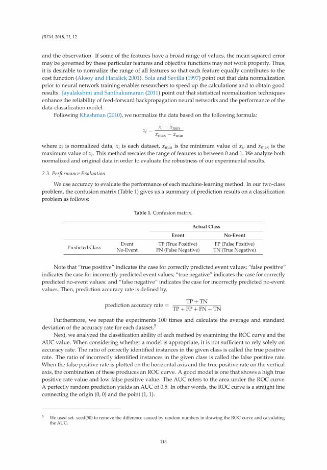
JRFM 2018, 11, 12
and the observation. If some of the features have a broad range of values, the mean squared errormay be governed by these particular features and objective functions may not work properly. Thus,it is desirable to normalize the range of all features so that each feature equally contributes to thecost function (Aksoy and Haralick 2001). Sola and Sevilla (1997) point out that data normalizationprior to neural network training enables researchers to speed up the calculations and to obtain goodresults. Jayalakshmi and Santhakumaran (2011) point out that statistical normalization techniquesenhance the reliability of feed-forward backpropagation neural networks and the performance of thedata-classification model.
Following Khashman (2010), we normalize the data based on the following formula:
zi =xi − xmin
xmax − xmin
where zi is normalized data, xi is each dataset, xmin is the minimum value of xi, and xmax is themaximum value of xi. This method rescales the range of features to between 0 and 1. We analyze bothnormalized and original data in order to evaluate the robustness of our experimental results.
2.3. Performance Evaluation
We use accuracy to evaluate the performance of each machine-learning method. In our two-classproblem, the confusion matrix (Table 1) gives us a summary of prediction results on a classificationproblem as follows:
Table 1. Confusion matrix.
Actual Class
Event No-Event
Predicted ClassEvent TP (True Positive) FP (False Positive)
No-Event FN (False Negative) TN (True Negative)
Note that “true positive” indicates the case for correctly predicted event values; “false positive”indicates the case for incorrectly predicted event values; “true negative” indicates the case for correctlypredicted no-event values: and “false negative” indicates the case for incorrectly predicted no-eventvalues. Then, prediction accuracy rate is defined by,
prediction accuracy rate =TP + TN
TP + FP + FN + TN
Furthermore, we repeat the experiments 100 times and calculate the average and standarddeviation of the accuracy rate for each dataset.5
Next, we analyzed the classification ability of each method by examining the ROC curve and theAUC value. When considering whether a model is appropriate, it is not sufficient to rely solely onaccuracy rate. The ratio of correctly identified instances in the given class is called the true positiverate. The ratio of incorrectly identified instances in the given class is called the false positive rate.When the false positive rate is plotted on the horizontal axis and the true positive rate on the verticalaxis, the combination of these produces an ROC curve. A good model is one that shows a high truepositive rate value and low false positive value. The AUC refers to the area under the ROC curve.A perfectly random prediction yields an AUC of 0.5. In other words, the ROC curve is a straight lineconnecting the origin (0, 0) and the point (1, 1).
5 We used set. seed(50) to remove the difference caused by random numbers in drawing the ROC curve and calculatingthe AUC.
113
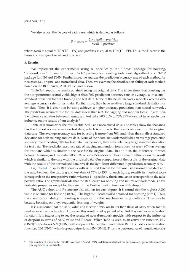
JRFM 2018, 11, 12
We also report the F-score of each case, which is defined as follows:
F − score =2 × recall × precision
recall + precision
where recall is equal to TP/(TP + FN) and precision is equal to TP/(TP +FP). Thus, the F-score is theharmonic average of recall and precision.
3. Results
We implement the experiments using R—specifically, the “ipred” package for bagging,“randomForest” for random forest, “ada” package for boosting (adaboost algorithm), and “h2o”package for NN and DNN. Furthermore, we analyze the prediction accuracy rate of each method fortwo cases i.e., original and normalized data. Then, we examine the classification ability of each methodbased on the ROC curve, AUC value, and F-score.
Table 2a,b report the results obtained using the original data. The tables show that boosting hasthe best performance and yields higher than 70% prediction accuracy rate on average, with a smallstandard deviation for both training and test data. None of the neural network models exceed a 70%average accuracy rate for test data. Furthermore, they have relatively large standard deviation fortest data. Thus, it is clear that boosting achieves a higher accuracy prediction than neural networks.The prediction accuracy rate for test data is less than 60% for bagging and random forest. In addition,the difference of ratios between training and test data (90%:10% or 75%:25%) does not have an obviousinfluence on the results of our analysis.6
Table 3a,b summarize the results obtained using normalized data. The tables show that boostinghas the highest accuracy rate on test data, which is similar to the results obtained for the originaldata case. The average accuracy rate for boosting is more than 70% and it has the smallest standarddeviation for both training and test data. None of the neural network models has an average predictionaccuracy rate exceeding 70% for test data. Furthermore, they have relatively large standard deviationfor test data. The prediction accuracy rate of bagging and random forest does not reach 60% on averagefor test date, which is similar to the case for the original data. In addition, the difference of ratiosbetween training and test data (90%:10% or 75%:25%) does not have a major influence on the result,which is similar to the case with the original data. Our comparison of the results of the original datawith the results of the normalized data reveals no significant difference in prediction accuracy rate.
Figures 1–11 display ROC curves with AUC and F-score for the case using normalized data andthe ratio between the training and test data of 75% to 25%. In each figure, sensitivity (vertical axis)corresponds to the true positive ratio, whereas 1—specificity (horizontal axis) corresponds to the falsepositive ratio. The graphs indicate that the ROC curve for boosting and neural network models havedesirable properties except for the case for the Tanh activation function with dropout.
The AUC values and F-score are also shown for each figure. It is found that the highest AUCvalue is obtained for boosting (0.769). The highest F-score is also obtained for boosting (0.744). Thus,the classification ability of boosting is superior to other machine-learning methods. This may bebecause boosting employs sequential learning of weights.
It is also found that the AUC value and F-score of NN are better than those of DNN when Tanh isused as an activation function. However, this result is not apparent when ReLU is used as an activationfunction. It is interesting to see the results of neural-network models with respect to the influenceof dropout in terms of AUC value and F-score. When Tanh is used as an activation function, NN(DNN) outperforms NN (DNN) with dropout. On the other hand, when ReLU is used as an activationfunction, NN (DNN) with dropout outperform NN (DNN). Thus the performance of neural networks
6 The number of units in the middle layers of NN and DNN is determined based on the Bayesian optimization method.(See Appendix A for details.)
114
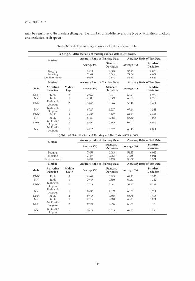
JRFM 2018, 11, 12
may be sensitive to the model setting i.e., the number of middle layers, the type of activation function,and inclusion of dropout.
Table 2. Prediction accuracy of each method for original data.
(a) Original data: the ratio of training and test data is 75% to 25%
MethodAccuracy Ratio of Training Data Accuracy Ratio of Test Data
Average (%)StandardDeviation
Average (%)StandardDeviation
Bagging 80.13 0.003 55.98 0.008Boosting 71.66 0.003 71.06 0.008
Random Forest 69.59 0.544 58.50 0.844
Method Accuracy Ratio of Training Data Accuracy Ratio of Test Data
ModelActivationFunction
MiddleLayer
Average (%)StandardDeviation
Average (%)StandardDeviation
DNN Tanh 2 70.66 0.721 68.93 0.972NN Tanh 1 71.01 0.569 69.59 0.778
DNN Tanh withDropout 2 58.47 3.566 58.46 3.404
NN Tanh withDropout 1 67.27 1.237 67.14 1.341
DNN ReLU 2 69.57 0.707 68.61 0.863NN ReLU 1 68.81 0.708 68.30 1.008
DNN ReLU withDropout 2 69.97 0.903 69.01 0.956
NN ReLU withDropout 1 70.12 0.637 69.48 0.881
(b) Original Data: the Ratio of Training and Test Data is 90% to 10%
MethodAccuracy Ratio of Training Data Accuracy Ratio of Test Data
Average (%)StandardDeviation
Average (%)StandardDeviation
Bagging 79.58 0.003 56.23 0.015Boosting 71.57 0.003 70.88 0.011
Random Forest 68.55 0.453 58.77 1.331
Method Accuracy Ratio of Training Data Accuracy Ratio of Test Data
ModelActivationFunction
MiddleLayer
Average (%)StandardDeviation
Average (%)StandardDeviation
DNN Tanh 2 69.64 0.683 69.31 1.325NN Tanh 1 70.49 0.550 69.61 1.312
DNN Tanh withDropout 2 57.29 3.681 57.27 4.117
NN Tanh withDropout 1 66.37 1.619 66.25 1.951
DNN ReLU 2 69.49 0.695 68.76 1.408NN ReLU 1 69.16 0.728 68.54 1.261
DNN ReLU withDropout 2 69.74 0.796 68.84 1.438
NN ReLU withDropout 1 70.26 0.573 69.55 1.210
115
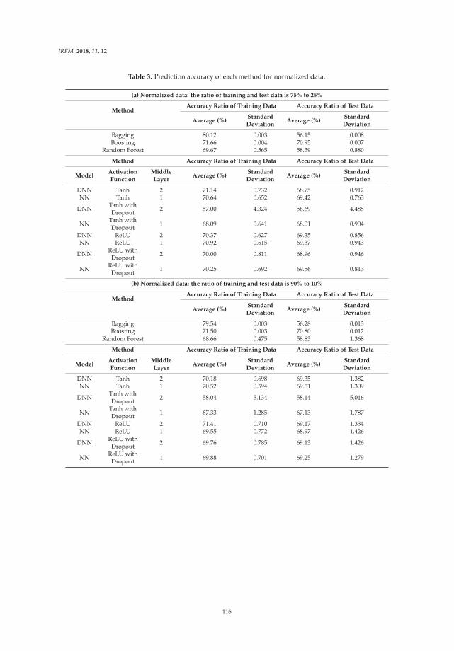
JRFM 2018, 11, 12
Table 3. Prediction accuracy of each method for normalized data.
(a) Normalized data: the ratio of training and test data is 75% to 25%
MethodAccuracy Ratio of Training Data Accuracy Ratio of Test Data
Average (%)StandardDeviation
Average (%)StandardDeviation
Bagging 80.12 0.003 56.15 0.008Boosting 71.66 0.004 70.95 0.007
Random Forest 69.67 0.565 58.39 0.880
Method Accuracy Ratio of Training Data Accuracy Ratio of Test Data
ModelActivationFunction
MiddleLayer
Average (%)StandardDeviation
Average (%)StandardDeviation
DNN Tanh 2 71.14 0.732 68.75 0.912NN Tanh 1 70.64 0.652 69.42 0.763
DNN Tanh withDropout 2 57.00 4.324 56.69 4.485
NN Tanh withDropout 1 68.09 0.641 68.01 0.904
DNN ReLU 2 70.37 0.627 69.35 0.856NN ReLU 1 70.92 0.615 69.37 0.943
DNN ReLU withDropout 2 70.00 0.811 68.96 0.946
NN ReLU withDropout 1 70.25 0.692 69.56 0.813
(b) Normalized data: the ratio of training and test data is 90% to 10%
MethodAccuracy Ratio of Training Data Accuracy Ratio of Test Data
Average (%)StandardDeviation
Average (%)StandardDeviation
Bagging 79.54 0.003 56.28 0.013Boosting 71.50 0.003 70.80 0.012
Random Forest 68.66 0.475 58.83 1.368
Method Accuracy Ratio of Training Data Accuracy Ratio of Test Data
ModelActivationFunction
MiddleLayer
Average (%)StandardDeviation
Average (%)StandardDeviation
DNN Tanh 2 70.18 0.698 69.35 1.382NN Tanh 1 70.52 0.594 69.51 1.309
DNN Tanh withDropout 2 58.04 5.134 58.14 5.016
NN Tanh withDropout 1 67.33 1.285 67.13 1.787
DNN ReLU 2 71.41 0.710 69.17 1.334NN ReLU 1 69.55 0.772 68.97 1.426
DNN ReLU withDropout 2 69.76 0.785 69.13 1.426
NN ReLU withDropout 1 69.88 0.701 69.25 1.279
116
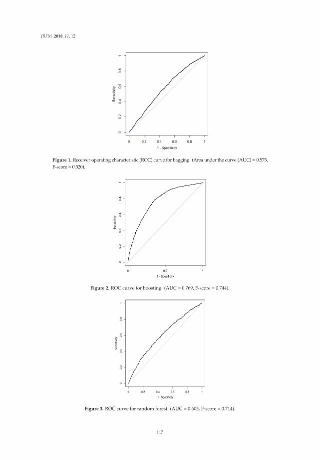
JRFM 2018, 11, 12
Figure 1. Receiver operating characteristic (ROC) curve for bagging. (Area under the curve (AUC) = 0.575,F-score = 0.520).
Figure 2. ROC curve for boosting. (AUC = 0.769, F-score = 0.744).
Figure 3. ROC curve for random forest. (AUC = 0.605, F-score = 0.714).
117
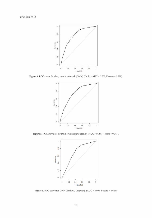
JRFM 2018, 11, 12
Figure 4. ROC curve for deep neural network (DNN) (Tanh). (AUC = 0.753, F-score = 0.721).
Figure 5. ROC curve for neural network (NN) (Tanh). (AUC = 0.768, F-score = 0.741).
Figure 6. ROC curve for DNN (Tanh w/Dropout). (AUC = 0.600, F-score = 0.620).
118
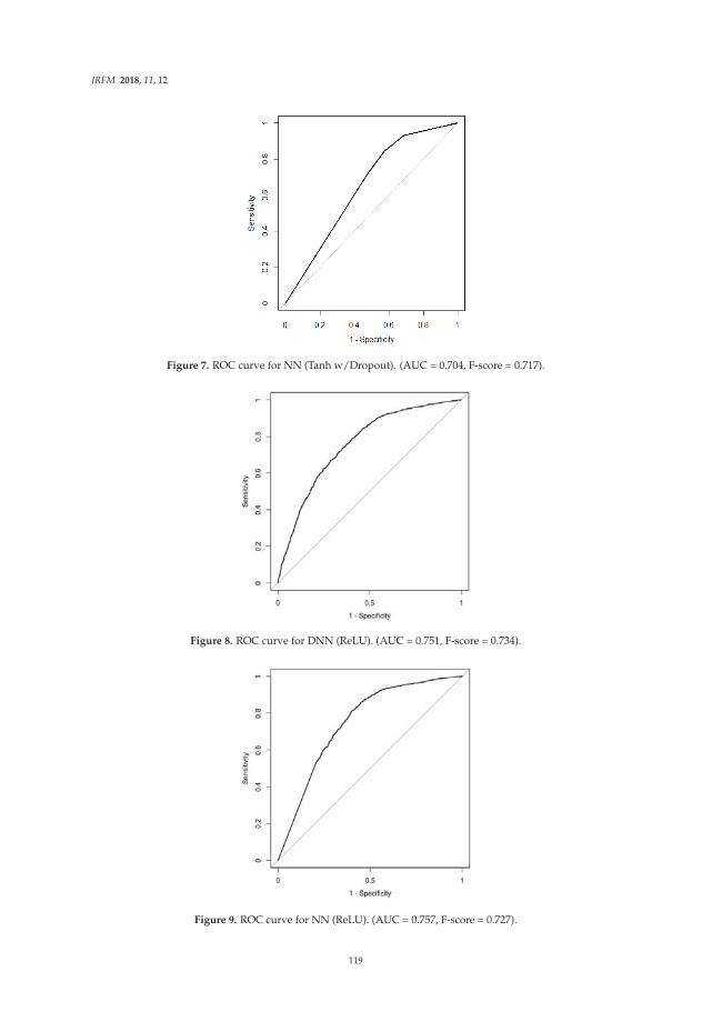
JRFM 2018, 11, 12
Figure 7. ROC curve for NN (Tanh w/Dropout). (AUC = 0.704, F-score = 0.717).
Figure 8. ROC curve for DNN (ReLU). (AUC = 0.751, F-score = 0.734).
Figure 9. ROC curve for NN (ReLU). (AUC = 0.757, F-score = 0.727).
119
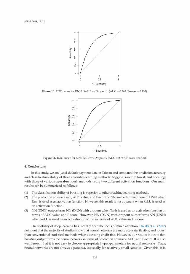
JRFM 2018, 11, 12
Figure 10. ROC curve for DNN (ReLU w/Dropout). (AUC = 0.765, F-score = 0.735).
Figure 11. ROC curve for NN (ReLU w/Dropout). (AUC = 0.767, F-score = 0.730).
4. Conclusions
In this study, we analyzed default payment data in Taiwan and compared the prediction accuracyand classification ability of three ensemble-learning methods: bagging, random forest, and boosting,with those of various neural-network methods using two different activation functions. Our mainresults can be summarized as follows:
(1) The classification ability of boosting is superior to other machine-learning methods.(2) The prediction accuracy rate, AUC value, and F-score of NN are better than those of DNN when
Tanh is used as an activation function. However, this result is not apparent when ReLU is used asan activation function.
(3) NN (DNN) outperforms NN (DNN) with dropout when Tanh is used as an activation function interms of AUC value and F-score. However, NN (DNN) with dropout outperforms NN (DNN)when ReLU is used as an activation function in terms of AUC value and F-score.
The usability of deep learning has recently been the focus of much attention. Oreski et al. (2012)point out that the majority of studies show that neural networks are more accurate, flexible, and robustthan conventional statistical methods when assessing credit risk. However, our results indicate thatboosting outperforms the neural network in terms of prediction accuracy, AUC, and F-score. It is alsowell known that it is not easy to choose appropriate hyper-parameters for neural networks. Thus,neural networks are not always a panacea, especially for relatively small samples. Given this, it is
120

JRFM 2018, 11, 12
worthwhile to make effective use of other methods such as boosting. Our future work will be to applya similar analysis to different data in order to check the robustness of our results.
Acknowledgments: We are grateful to the three anonymous referees for their helpful comments and suggestions.An early version of this paper was read at the Workshop of Big Data and Machine Learning. We are gratefulto Zheng Zhang and Xiao Jing Cai for helpful comments and suggestions. This research was supported bya grant-in-aid from The Nihon Hoseigakkai Foundation.
Author Contributions: Shigeyuki Hamori conceived and designed the experiments; Minami Kawai, Takahiro Kume,Yuji Murakami and Chikara Watanabe performed the experiments, analyzed the data, and contributedreagents/materials/analysis tools; and Shigeyuki Hamori, Minami Kawai, Takahiro Kume, Yuji Murakami andChikara Watanabe wrote the paper.
Conflicts of Interest: The authors declare no conflicts of interest. The founding sponsors had no role in the designof the study; in the collection, analyses, or interpretation of data; in the writing of the manuscript, or in thedecision to publish the results.
Appendix A. Results of Bayesian Optimization
Table A1. Number of units in middle layer for NN.
Method DataRatio of
Training andTest Data (%)
Input Layer Middle Layer Output Layer
Tanh Original 75:25 23 7 2Tanh Original 90:10 23 5 2
Tanh with Dropout Original 75:25 23 14 2Tanh with Dropout Original 90:10 23 12 2
ReLU Original 75:25 23 3 2ReLU Original 90:10 23 7 2
ReLU with Dropout Original 75:25 23 14 2ReLU with Dropout Original 90:10 23 19 2
Tanh Normalized 75:25 23 5 2Tanh Normalized 90:10 23 5 2
Tanh with Dropout Normalized 75:25 23 5 2Tanh with Dropout Normalized 90:10 23 10 2
ReLU Normalized 75:25 23 11 2ReLU Normalized 90:10 23 4 2
ReLU with Dropout Normalized 75:25 23 16 2ReLU with Dropout Normalized 90:10 23 12 2
Table A2. Number of units in middle layers for DNN.
Method DataRatio of
Training andTest Data (%)
Input LayerMiddleLayer 1
MiddleLayer 2
OutputLayer
Tanh Original 75:25 23 5 17 2Tanh Original 90:10 23 2 9 2
Tanh with Dropout Original 75:25 23 9 7 2Tanh with Dropout Original 90:10 23 3 11 2
ReLU Original 75:25 23 4 6 2ReLU Original 90:10 23 4 9 2
ReLU with Dropout Original 75:25 23 13 9 2ReLU with Dropout Original 90:10 23 5 20 2
Tanh Normalized 75:25 23 6 17 2Tanh Normalized 90:10 23 4 3 2
Tanh with Dropout Normalized 75:25 23 9 4 2Tanh with Dropout Normalized 90:10 23 3 18 2
ReLU Normalized 75:25 23 4 6 2ReLU Normalized 90:10 23 10 7 2
ReLU with Dropout Normalized 75:25 23 16 9 2ReLU with Dropout Normalized 90:10 23 5 21 2
121

JRFM 2018, 11, 12
References
Aksoy, Selim, and Robert M. Haralick. 2001. Feature normalization and likelihood-based similarity measures forimage retrieval. Pattern Recognition. Letters 22: 563–82. [CrossRef]
Angelini, Eliana, Giacomo di Tollo, and Andrea Roli. 2008. A neural network approach for credit risk evaluation.Quarterly Review of Economics and Finance 48: 733–55. [CrossRef]
Boguslauskas, Vytautas, and Ricardas Mileris. 2009. Estimation of credit risks by artificial neural networks models.Izinerine Ekonomika-Engerrring Economics 4: 7–14.
Breiman, Leo. 1996. Bagging predictors. Machine Learning 24: 123–40. [CrossRef]Breiman, Leo. 2001. Random forests. Machine Learning 45: 5–32. [CrossRef]Freund, Yoav, and Robert E. Schapire. 1996. Experiments with a new boosting algorithm. Paper presented at the
Thirteenth International Conference on Machine Learning, Bari, Italy, July 3–6; pp. 148–56.Gante, Dionicio D., Bobby D. Gerardo, and Bartolome T. Tanguilig. 2015. Neural network model using back
propagation algorithm for credit risk evaluation. Paper presented at the 3rd International Conference onArtificial Intelligence and Computer Science (AICS2015), Batu Ferringhi, Penang, Malaysia, October 12–13;pp. 12–13.
Jayalakshmi, T., and A. Santhakumaran. 2011. Statistical Normalization and Back Propagation for Classification.International Journal of Computer Theory and Engineering 3: 83–93.
Khashman, Adnan. 2010. Neural networks for credit risk evaluation: Investigation of different neural models andlearning schemes. Expert Systems with Applications 37: 6233–39. [CrossRef]
Khemakhem, Sihem, and Younes Boujelbene. 2015. Credit risk prediction: A comparative study betweendiscriminant analysis and the neural network approach. Accounting and Management Information Systems 14:60–78.
Khshman, Adnan. 2009. A neural network model for credit risk evaluation. International Journal of Neural Systems19: 285–94. [CrossRef] [PubMed]
Lantz, Brett. 2015. Machine Learning with R, 2nd ed. Birmingham: Packt Publishing Ltd.LeCun, Yann, Yoshua Bengio, and Geoffrey Hinton. 2015. Deep learning. Nature 521: 436–44. [CrossRef] [PubMed]Oreski, Stjepan, Dijana Oreski, and Goran Oreski. 2012. Hybrid system with genetic algorithm and artificial neural
networks and its application to retail credit risk assessment. Expert Systems with Applications 39: 12605–17.[CrossRef]
Schapire, Robert E. 1999. A brief introduction to boosting. Paper presented at the Sixteenth International JointConference on Artificial Intelligence, Stockholm, Sweden, July 31–August 6; pp. 1–6.
Shapire, Robert E., and Yoav Freund. 2012. Boosting: Foundations and Algorithms. Cambridge: The MIT Press.Sola, J., and Joaquin Sevilla. 1997. Importance of input data normalization for the application of neural networks
to complex industrial problems. IEEE Transactions on Nuclear Science 44: 1464–68. [CrossRef]Srivastava, Nitish, Georey Hinton, Alex Krizhevsky, Ilya Sutskever, and Ruslan Salakhutdinov. 2014. Dropout:
A simple way to prevent neural networks from overfitting. Journal of Machine Learning Research 15: 1929–58.Yeh, I-Cheng, and Che-hui Lien. 2009. The comparisons of data mining techniques for the predictive accuracy of
probability of default of credit card clients. Expert Systems with Applications 36: 2473–80. [CrossRef]
© 2018 by the authors. Licensee MDPI, Basel, Switzerland. This article is an open accessarticle distributed under the terms and conditions of the Creative Commons Attribution(CC BY) license (http://creativecommons.org/licenses/by/4.0/).
122
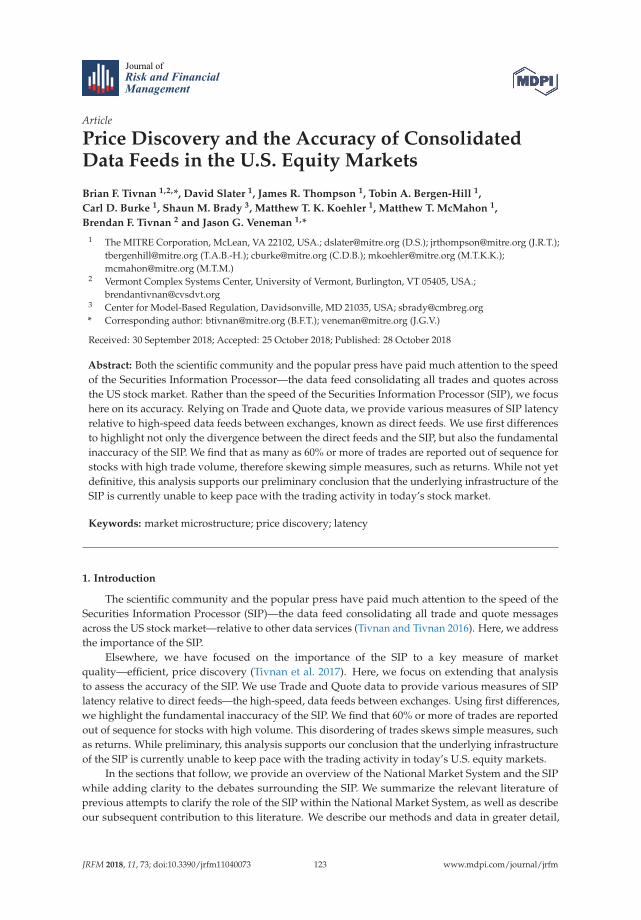
Journal of
Risk and FinancialManagement
Article
Price Discovery and the Accuracy of ConsolidatedData Feeds in the U.S. Equity Markets
Brian F. Tivnan 1,2,*, David Slater 1, James R. Thompson 1, Tobin A. Bergen-Hill 1,
Carl D. Burke 1, Shaun M. Brady 3, Matthew T. K. Koehler 1, Matthew T. McMahon 1,
Brendan F. Tivnan 2 and Jason G. Veneman 1,*
1 The MITRE Corporation, McLean, VA 22102, USA.; [email protected] (D.S.); [email protected] (J.R.T.);[email protected] (T.A.B.-H.); [email protected] (C.D.B.); [email protected] (M.T.K.K.);[email protected] (M.T.M.)
2 Vermont Complex Systems Center, University of Vermont, Burlington, VT 05405, USA.;[email protected]
3 Center for Model-Based Regulation, Davidsonville, MD 21035, USA; [email protected]* Corresponding author: [email protected] (B.F.T.); [email protected] (J.G.V.)
Received: 30 September 2018; Accepted: 25 October 2018; Published: 28 October 2018
Abstract: Both the scientific community and the popular press have paid much attention to the speedof the Securities Information Processor—the data feed consolidating all trades and quotes acrossthe US stock market. Rather than the speed of the Securities Information Processor (SIP), we focushere on its accuracy. Relying on Trade and Quote data, we provide various measures of SIP latencyrelative to high-speed data feeds between exchanges, known as direct feeds. We use first differencesto highlight not only the divergence between the direct feeds and the SIP, but also the fundamentalinaccuracy of the SIP. We find that as many as 60% or more of trades are reported out of sequence forstocks with high trade volume, therefore skewing simple measures, such as returns. While not yetdefinitive, this analysis supports our preliminary conclusion that the underlying infrastructure of theSIP is currently unable to keep pace with the trading activity in today’s stock market.
Keywords: market microstructure; price discovery; latency
1. Introduction
The scientific community and the popular press have paid much attention to the speed of theSecurities Information Processor (SIP)—the data feed consolidating all trade and quote messagesacross the US stock market—relative to other data services (Tivnan and Tivnan 2016). Here, we addressthe importance of the SIP.
Elsewhere, we have focused on the importance of the SIP to a key measure of marketquality—efficient, price discovery (Tivnan et al. 2017). Here, we focus on extending that analysisto assess the accuracy of the SIP. We use Trade and Quote data to provide various measures of SIPlatency relative to direct feeds—the high-speed, data feeds between exchanges. Using first differences,we highlight the fundamental inaccuracy of the SIP. We find that 60% or more of trades are reportedout of sequence for stocks with high volume. This disordering of trades skews simple measures, suchas returns. While preliminary, this analysis supports our conclusion that the underlying infrastructureof the SIP is currently unable to keep pace with the trading activity in today’s U.S. equity markets.
In the sections that follow, we provide an overview of the National Market System and the SIPwhile adding clarity to the debates surrounding the SIP. We summarize the relevant literature ofprevious attempts to clarify the role of the SIP within the National Market System, as well as describeour subsequent contribution to this literature. We describe our methods and data in greater detail,
JRFM 2018, 11, 73; doi:10.3390/jrfm11040073 www.mdpi.com/journal/jrfm123

JRFM 2018, 11, 73
followed by a presentation of our findings. We then conclude the paper with a brief discussion of theimplications of our findings.
Overview of the National Market System
The National Market System (colloquially known as the “stock market”) includes all market centerswhere investors can buy and sell shares of publicly traded companies. To facilitate the efficient exchange ofcapital and shares in the National Market System (NMS), each market center is required to publish boththe Best Bid (i.e., the highest price at which an investor is willing to pay for a single share of a given stock)and the Best Offer (i.e., the lowest price at which an investor is willing to sell a single share of a givenstock), as well as how many shares the investor is willing to sell at that price. Across the entirety of theNMS, the highest bid and the lowest offer comprise what is known as the National Best Bid and Offer(NBBO) and the difference between the Best Bid and Best Offer is known as the spread.
The NBBO reflects a distillation of the order flow across all the stock exchanges comprising theNMS. Figure 1 provides a graphical depiction of the three major datacenters of the NMS, all of which arelocated in northern New Jersey. Table A1 in the Appendix A also depicts the distribution of the familiesof exchanges across these datacenters. As depicted in Figure 1, the communications infrastructureconnects the datacenters by dedicated, high-speed networks known as Direct Feeds depicted in redand black, as well as by the Security Information Processor depicted in pink. The Direct Feeds providehigh-speed communications channels (e.g., faster than 50% of the speed of light (Angel 2014)) whereall orders flow between the exchanges. The Securities Information Processor, or SIP, consolidates anddistills all the order flow from the Direct Feeds to determine and disseminate the NBBO, as well asreport all completed trades. We developed and posted an animation to provide a more illustrativedepiction of these interactive dynamics between the direct feeds and the SIP1.
Figure 1. Graphical depiction of the three major market centers in the National Market System (NMS).SIP, Securities Information Processor.
We conclude this overview of the National Market System with a description of the two TradeReporting Facilities; namely, the NYSE Trade Reporting Facility (NTRF) and the NASDAQ TradeReporting Facility (QTRF). Both Trade Reporting Facilities consolidate the trade reports from allAlternative Trading Systems (colloquially known as “Dark Pools”). The NTRF consolidates DarkPool trade reports of NYSE-listed stocks whereas the QTRF consolidates Dark Pool trade reports ofNASDAQ-listed stocks.
1 The MITRE Corporation. “An Example of High Frequency Trader (HFT) Latency Arbitrage.” https://www.youtube.com/watch?v=1ltjnbBaFok&feature=youtu.be. Date of information retrieval: 30 September 2018.
124
JRFM 2018, 11, 73
Unlike an exchange, which must display best, local quotes, a Dark Pool is a market center wheretrading occurs without displaying any local quotes. Prevailing regulations still require that pricediscovery at Dark Pools are driven by the NBBO—same as at each exchange. While not depicted inFigure 1, we include Dark Pools here in our analysis for completeness, since trade reports from DarkPools contribute to the overall, message traffic consolidated and disseminated by the SIP.
2. Review of Relevant Literature
There is widespread agreement that Mandelbrot (1963) was one of the first to characterize thedynamic behavior of prices in modern markets; later to be extended by Cont (2001). A related study(Johnson et al. 2012, 2013) identified some anomalous behavior in the dynamics of market prices,which deviated from previous expectations (Mandelbrot 1963; Cont 2001). At the time, however,the resolution of our data prevented us from making any definitive determinations about the causalmechanisms of these behaviors.
Initially in the press and later in his book, Scott Patterson was one of the first to draw attention tothe speed discrepancy between the SIP and the direct feeds (Patterson 2012a, 2012b), only later to befollowed in 2014 by Michael Lewis’ (Lewis 2014) popular book, Flash Boys. Neither of these authorsfully explored the implications of the speed discrepancy, instead relying heavily upon the works offinancial industry practitioners.
A few industry practitioners were the first to identify the speed discrepancy between that of theSIP and the direct feeds. Arnuk and Saluzzi (2012) were one of the first to highlight these latencydiscrepancies. Bodek (2013) detailed the sweeping changes instituted by RegNMS, changes whichstimulated the technological arms race and the insatiable demand for greater speeds from the directfeeds. Furthermore, Nanex Research (2014a) highlighted the spoils, which can be extracted in specificinstances by those market participants so fortunate as to subscribe to the direct feeds.
Scientific contributions to this debate have been preliminary, possibly due to the limitedavailability of authoritative data within the scientific community. While authoritative datasets exist,subscriptions to them are extraordinarily expensive and therefore largely available only to specialized,market participants along with regulatory agencies.
Ding et al. (2014) provide one of the first scientific analyses of direct feed and SIP latencies.More recently, Bartlett and McCrary (2017) attempted to revise and generalize earlier findings(Nanex Research 2014a) by quantifying the total profits from subscribing to the direct feeds.
One common theme prevails throughout these analyses: The implication that the SIP accuratelydepicts market dynamics, albeit subject to some latency. We address this limitation of previous studiesby highlighting and quantifying the inaccuracies of the SIP.
3. Methods
The implications of ever increasing market speeds can be a difficult topic to understand evenfor those immersed in market data daily. The following is an attempt to break down some empiricalanalyses on granular data from US stock markets that illustrate some of the implications from SIPlatencies and the subsequent impact on the accuracy of the SIP. We rely on Trade and Quote dataspanning the National Market System. More precisely, we purchased the NxCore dataset from NanexResearch for the following periods: The calendar year 2014, and the second and third quarters of 2015.
Many of the subsequent examples stem from market activity on a representative day (i.e.,11 August 2015), which we chose for three reasons. First, 11 August 2015 was a not a noteworthy dayin the U.S. equity markets (i.e., the absence of any market-wide events). Second, this representativeday closely precedes a notable day in the U.S. equity markets (i.e., 24 August 2015), which is knowncolloquially as “Manic Monday.” Third, there were no announced modifications to the SIP between11 August and 24 August. Given these three reasons above, it is realistic to assume the sameunderlying, market infrastructure for both days. Therefore, 11 August 2015 serves as a useful proxyfor a representative day in the U.S. equity markets.
125
JRFM 2018, 11, 73
We capture both breadth and depth in our analyses. We achieve breadth in two ways.First, we analyzed the entire population of the 7993 unique tickers (i.e., stocks and exchange-tradedfunds) that printed quotes and trade reports to the SIP on the representative day. The reader willnote that an exchange-traded fund (ETF) is a security similar to a mutual fund, but an ETF tradesthroughout the day in the same manner as a stock. Second, we also closely analyzed SPY (i.e., the SPDRS&P 500 ETF). It is important to note that the SPY is often used as a proxy of the U.S. equity market.Unlike the S P 500 index, which cannot be directly traded, the SPY represents one of the largest andmost liquid, market-wide securities. For the SPY, we analyzed price, spread and market crosses.A special case of the spread occurs when the spread becomes negative. Such instances of a negativespread for the NBBO depict a crossed market, or simply cross for short. While a small spread indicatesgeneral agreement on price across all market participants, a large spread and crosses indicate littleagreement on price. Both large spreads and crosses are indicators of inefficient, price discovery.
We also achieve depth of our analysis in a comprehensive manner. Rather than limiting ouranalyses to any one stock or relying solely on the large-cap stocks that comprise the Dow 30 asin previous studies (Bartlett and McCrary 2017), we chose a convenience sample of 14 stocks.This heterogeneous set of stocks varies on market capitalization, listed exchange and trading volume.This sample ranges from Apple (i.e., stock ticker: AAPL), one of the largest and most actively tradedstocks in the world to Acme United Corporation (i.e., stock ticker: ACU), which is a lightly traded,small-cap stock.
Our analyses include some depictions of common descriptive measures of market performance,namely price and trade volume, as well as the monetary value of that trading activity. We thende-construct this market activity by specific exchange and components of the SIP.
We continue our analyses with a focus on the latencies between the direct feeds and the SIP,beginning with simple counts and frequency distributions. We extend this analysis by comparing firstdifferences to highlight the divergence between the direct feeds and the SIP. We conclude with ananalysis of these measures for comparison with known market events.
4. Results
As described above, we begin with empirical evidence confirming our focal date as arepresentative day in the U.S. equity markets. From there, we provide depictions of commondescriptive measures of market performance. We then de-construct this market activity by specificexchange and components of the SIP. We then present our analysis of first differences to highlight thedivergence between the direct feeds and the SIP. We conclude with an analysis of these measures forcomparison with known, market events.
4.1. Representative Day in the U.S. Equity Markets
For simplicity and clarity in the presentation of our analyses, we chose a representative day in theU.S. equity markets (i.e., 11 August 2015) for its distinction from a noteworthy day (i.e., 24 August2015) within only a two-week span. Figures 2 and 3 provide the empirical evidence to support thisdistinction. Both figures plot the price, spread and market crosses for SPY.
Figure 2 depicts the market dynamics for SPY on 24 August 2015. Leading up to and throughthe opening of the market day, the widening spread and frequent crosses indicate a tremendousuncertainty of the price. Even as spreads narrowed and price stabilized throughout the market day,frequent crosses persisted. These are all indicators of inefficient, price discovery.
Figure 3 depicts the market dynamics for SPY on 11 August 2015. Unlike the dynamics of “ManicMonday,” Figure 3 reflects a “typical market day.” More precisely, spreads remain small throughoutthe market day and crosses are intermittent yet fleeting while price is largely stable. Moreover, Figure 3provides no evidence that would lead one to conclude that the underlying, market infrastructure isoverwhelmed in any meaningful way on this day.
126
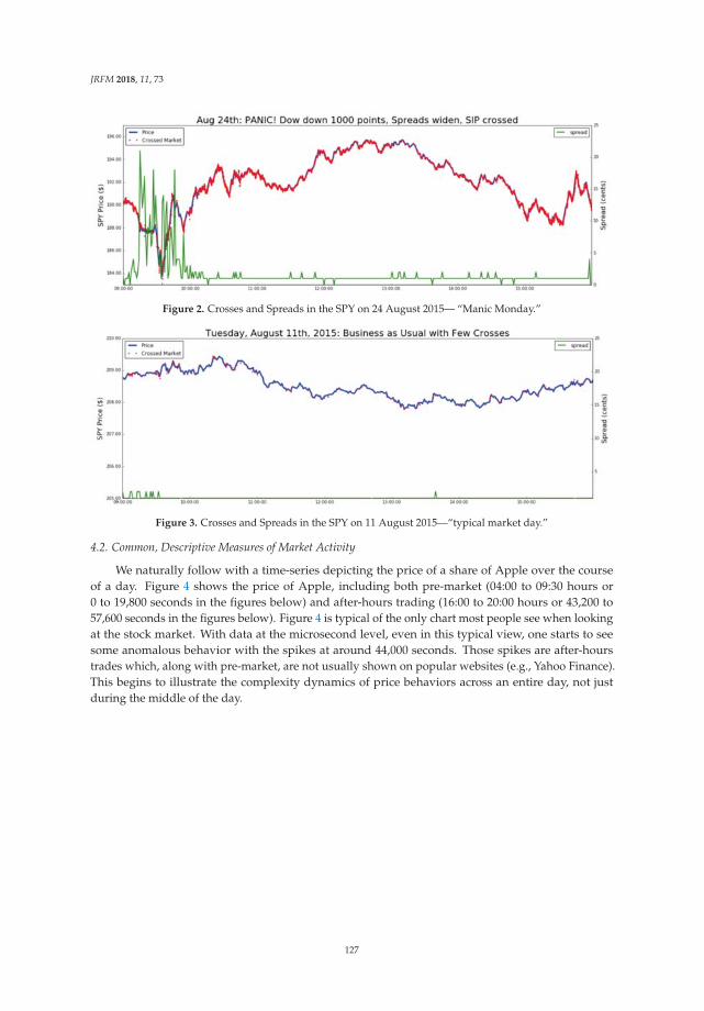
JRFM 2018, 11, 73
Figure 2. Crosses and Spreads in the SPY on 24 August 2015— “Manic Monday.”
Figure 3. Crosses and Spreads in the SPY on 11 August 2015—“typical market day.”
4.2. Common, Descriptive Measures of Market Activity
We naturally follow with a time-series depicting the price of a share of Apple over the courseof a day. Figure 4 shows the price of Apple, including both pre-market (04:00 to 09:30 hours or0 to 19,800 seconds in the figures below) and after-hours trading (16:00 to 20:00 hours or 43,200 to57,600 seconds in the figures below). Figure 4 is typical of the only chart most people see when lookingat the stock market. With data at the microsecond level, even in this typical view, one starts to seesome anomalous behavior with the spikes at around 44,000 seconds. Those spikes are after-hourstrades which, along with pre-market, are not usually shown on popular websites (e.g., Yahoo Finance).This begins to illustrate the complexity dynamics of price behaviors across an entire day, not justduring the middle of the day.
127
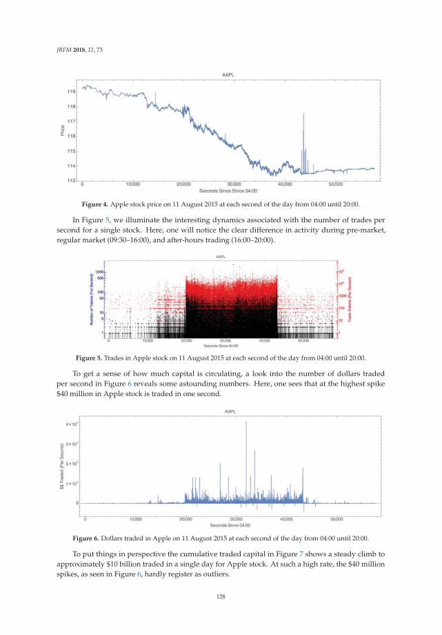
JRFM 2018, 11, 73
Figure 4. Apple stock price on 11 August 2015 at each second of the day from 04:00 until 20:00.
In Figure 5, we illuminate the interesting dynamics associated with the number of trades persecond for a single stock. Here, one will notice the clear difference in activity during pre-market,regular market (09:30–16:00), and after-hours trading (16:00–20:00).
Figure 5. Trades in Apple stock on 11 August 2015 at each second of the day from 04:00 until 20:00.
To get a sense of how much capital is circulating, a look into the number of dollars tradedper second in Figure 6 reveals some astounding numbers. Here, one sees that at the highest spike$40 million in Apple stock is traded in one second.
Figure 6. Dollars traded in Apple on 11 August 2015 at each second of the day from 04:00 until 20:00.
To put things in perspective the cumulative traded capital in Figure 7 shows a steady climb toapproximately $10 billion traded in a single day for Apple stock. At such a high rate, the $40 millionspikes, as seen in Figure 6, hardly register as outliers.
128
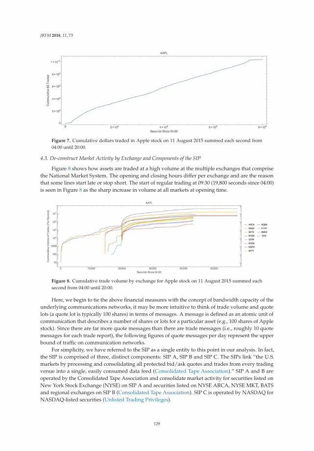
JRFM 2018, 11, 73
Figure 7. Cumulative dollars traded in Apple stock on 11 August 2015 summed each second from04:00 until 20:00.
4.3. De-construct Market Activity by Exchange and Components of the SIP
Figure 8 shows how assets are traded at a high volume at the multiple exchanges that comprisethe National Market System. The opening and closing hours differ per exchange and are the reasonthat some lines start late or stop short. The start of regular trading at 09:30 (19,800 seconds since 04:00)is seen in Figure 8 as the sharp increase in volume at all markets at opening time.
Figure 8. Cumulative trade volume by exchange for Apple stock on 11 August 2015 summed eachsecond from 04:00 until 20:00.
Here, we begin to tie the above financial measures with the concept of bandwidth capacity of theunderlying communications networks, it may be more intuitive to think of trade volume and quotelots (a quote lot is typically 100 shares) in terms of messages. A message is defined as an atomic unit ofcommunication that describes a number of shares or lots for a particular asset (e.g., 100 shares of Applestock). Since there are far more quote messages than there are trade messages (i.e., roughly 10 quotemessages for each trade report), the following figures of quote messages per day represent the upperbound of traffic on communication networks.
For simplicity, we have referred to the SIP as a single entity to this point in our analysis. In fact,the SIP is comprised of three, distinct components: SIP A, SIP B and SIP C. The SIPs link “the U.S.markets by processing and consolidating all protected bid/ask quotes and trades from every tradingvenue into a single, easily consumed data feed (Consolidated Tape Association).” SIP A and B areoperated by the Consolidated Tape Association and consolidate market activity for securities listed onNew York Stock Exchange (NYSE) on SIP A and securities listed on NYSE ARCA, NYSE MKT, BATSand regional exchanges on SIP B (Consolidated Tape Association). SIP C is operated by NASDAQ forNASDAQ-listed securities (Unlisted Trading Privileges).
129

JRFM 2018, 11, 73
In Figure 9, one can again clearly see the opening and closing of the regular market day. Figure 9shows messages that are recorded at each of the three SIPs. During the market day, there are very fewinstances that less than 1000 messages per second are printed to the SIPs, while there are times, such asthe market open and close, when message traffic exceeds 100,000 messages per second.
Figure 9. Quote messages by SIP for Apple stock on 11 August 2015 for each second from 04:00 until 20:00.
4.4. Latencies between the Direct Feeds and the SIP
Recall that the SIP exists to unify the market in time via efficient discovery of equity prices. To geta picture of how long it takes for trades to go from being reported at an exchange to being aggregatedand recorded by the SIP for all market participants to see, one can look at the SIP latency. Latency isdefined here by the timestamp from the SIP minus the timestamp from when the reporting exchangesent the trade or quote information to the SIP. The latency in microseconds for trades at each of thethree SIPs for all stocks is shown in Figures 10–12.
From these three figures, one can see that the median, standard deviation and range in latencyare similar across each SIP. The median latencies across all SIPs and all exchanges are within 700 μs ofeach other. From this, one might infer that trade reporting latencies are similar.
While similarities in latency median, standard deviation and range certainly do exist, there are atleast two exceptions to these similarities. The first exception is the Chicago Stock Exchange (CHX).It was first reported elsewhere that CHX latencies are outliers from that of the other exchanges, as wellas that CHX has limited share of the trading volume despite often contributing to efficient, pricediscovery (Nanex Research 2014b). Our findings here confirm CHX latencies as outliers. The secondexception relates to the NTRF where Dark Pool trades are consolidated for NYSE-listed stocks.
130
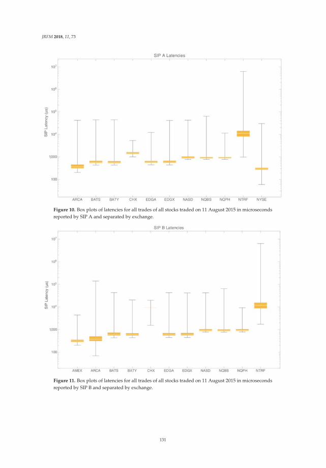
JRFM 2018, 11, 73
Figure 10. Box plots of latencies for all trades of all stocks traded on 11 August 2015 in microsecondsreported by SIP A and separated by exchange.
Figure 11. Box plots of latencies for all trades of all stocks traded on 11 August 2015 in microsecondsreported by SIP B and separated by exchange.
131
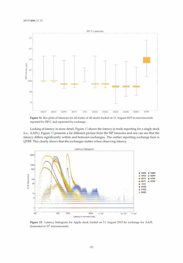
JRFM 2018, 11, 73
Figure 12. Box plots of latencies for all trades of all stocks traded on 11 August 2015 in microsecondsreported by SIP C and separated by exchange.
Looking at latency in more detail, Figure 13 shows the latency in trade reporting for a single stock(i.e., AAPL). Figure 13 presents a far different picture from the SIP latencies and one can see that thelatency differs significantly within and between exchanges. The outlier reporting exchange here isQTRF. This clearly shows that the exchanges matter when observing latency.
Figure 13. Latency histogram for Apple stock traded on 11 August 2015 by exchange for AAPL(truncated at 105 microseconds).
132
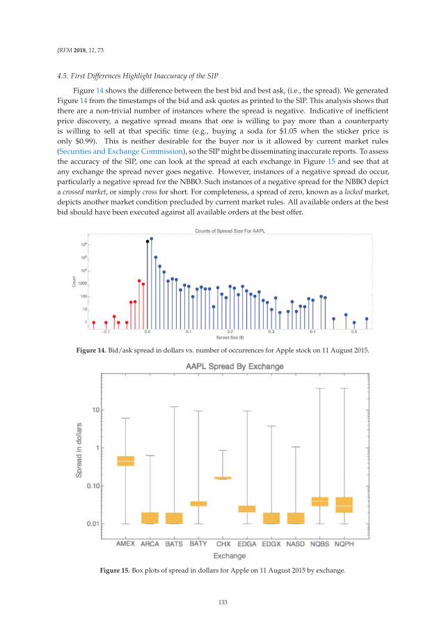
JRFM 2018, 11, 73
4.5. First Differences Highlight Inaccuracy of the SIP
Figure 14 shows the difference between the best bid and best ask, (i.e., the spread). We generatedFigure 14 from the timestamps of the bid and ask quotes as printed to the SIP. This analysis shows thatthere are a non-trivial number of instances where the spread is negative. Indicative of inefficientprice discovery, a negative spread means that one is willing to pay more than a counterpartyis willing to sell at that specific time (e.g., buying a soda for $1.05 when the sticker price isonly $0.99). This is neither desirable for the buyer nor is it allowed by current market rules(Securities and Exchange Commission), so the SIP might be disseminating inaccurate reports. To assessthe accuracy of the SIP, one can look at the spread at each exchange in Figure 15 and see that atany exchange the spread never goes negative. However, instances of a negative spread do occur,particularly a negative spread for the NBBO. Such instances of a negative spread for the NBBO depicta crossed market, or simply cross for short. For completeness, a spread of zero, known as a locked market,depicts another market condition precluded by current market rules. All available orders at the bestbid should have been executed against all available orders at the best offer.
Figure 14. Bid/ask spread in dollars vs. number of occurrences for Apple stock on 11 August 2015.
Figure 15. Box plots of spread in dollars for Apple on 11 August 2015 by exchange.
133
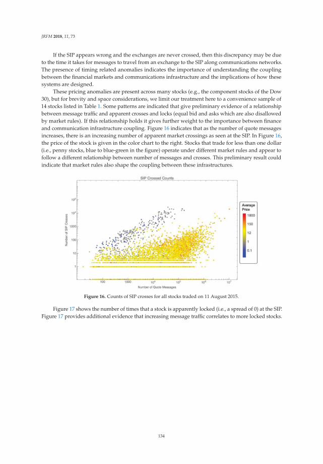
JRFM 2018, 11, 73
If the SIP appears wrong and the exchanges are never crossed, then this discrepancy may be dueto the time it takes for messages to travel from an exchange to the SIP along communications networks.The presence of timing related anomalies indicates the importance of understanding the couplingbetween the financial markets and communications infrastructure and the implications of how thesesystems are designed.
These pricing anomalies are present across many stocks (e.g., the component stocks of the Dow30), but for brevity and space considerations, we limit our treatment here to a convenience sample of14 stocks listed in Table 1. Some patterns are indicated that give preliminary evidence of a relationshipbetween message traffic and apparent crosses and locks (equal bid and asks which are also disallowedby market rules). If this relationship holds it gives further weight to the importance between financeand communication infrastructure coupling. Figure 16 indicates that as the number of quote messagesincreases, there is an increasing number of apparent market crossings as seen at the SIP. In Figure 16,the price of the stock is given in the color chart to the right. Stocks that trade for less than one dollar(i.e., penny stocks, blue to blue-green in the figure) operate under different market rules and appear tofollow a different relationship between number of messages and crosses. This preliminary result couldindicate that market rules also shape the coupling between these infrastructures.
Figure 16. Counts of SIP crosses for all stocks traded on 11 August 2015.
Figure 17 shows the number of times that a stock is apparently locked (i.e., a spread of 0) at the SIP.Figure 17 provides additional evidence that increasing message traffic correlates to more locked stocks.
134
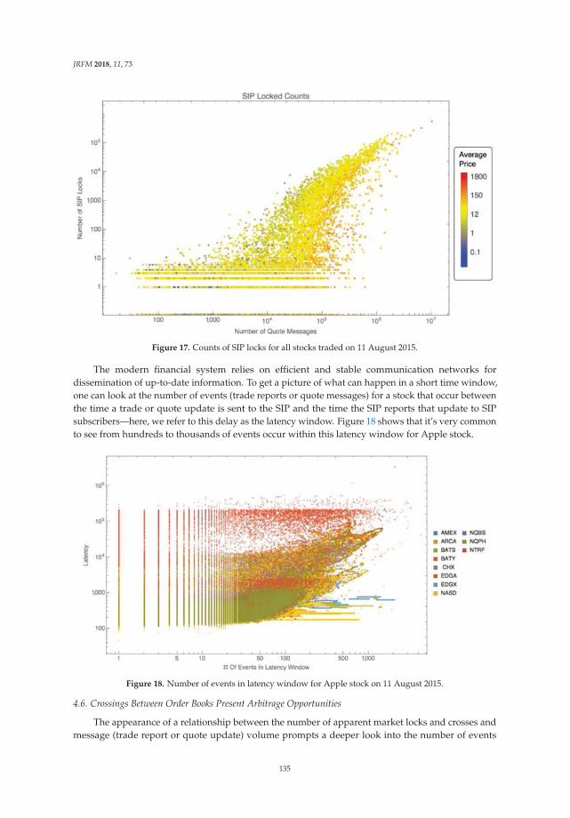
JRFM 2018, 11, 73
Figure 17. Counts of SIP locks for all stocks traded on 11 August 2015.
The modern financial system relies on efficient and stable communication networks fordissemination of up-to-date information. To get a picture of what can happen in a short time window,one can look at the number of events (trade reports or quote messages) for a stock that occur betweenthe time a trade or quote update is sent to the SIP and the time the SIP reports that update to SIPsubscribers—here, we refer to this delay as the latency window. Figure 18 shows that it’s very commonto see from hundreds to thousands of events occur within this latency window for Apple stock.
Figure 18. Number of events in latency window for Apple stock on 11 August 2015.
4.6. Crossings Between Order Books Present Arbitrage Opportunities
The appearance of a relationship between the number of apparent market locks and crosses andmessage (trade report or quote update) volume prompts a deeper look into the number of events
135
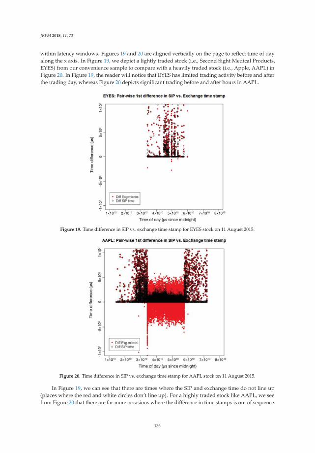
JRFM 2018, 11, 73
within latency windows. Figures 19 and 20 are aligned vertically on the page to reflect time of dayalong the x axis. In Figure 19, we depict a lightly traded stock (i.e., Second Sight Medical Products,EYES) from our convenience sample to compare with a heavily traded stock (i.e., Apple, AAPL) inFigure 20. In Figure 19, the reader will notice that EYES has limited trading activity before and afterthe trading day, whereas Figure 20 depicts significant trading before and after hours in AAPL.
Figure 19. Time difference in SIP vs. exchange time stamp for EYES stock on 11 August 2015.
Figure 20. Time difference in SIP vs. exchange time stamp for AAPL stock on 11 August 2015.
In Figure 19, we can see that there are times where the SIP and exchange time do not line up(places where the red and white circles don’t line up). For a highly traded stock like AAPL, we seefrom Figure 20 that there are far more occasions where the difference in time stamps is out of sequence.
136
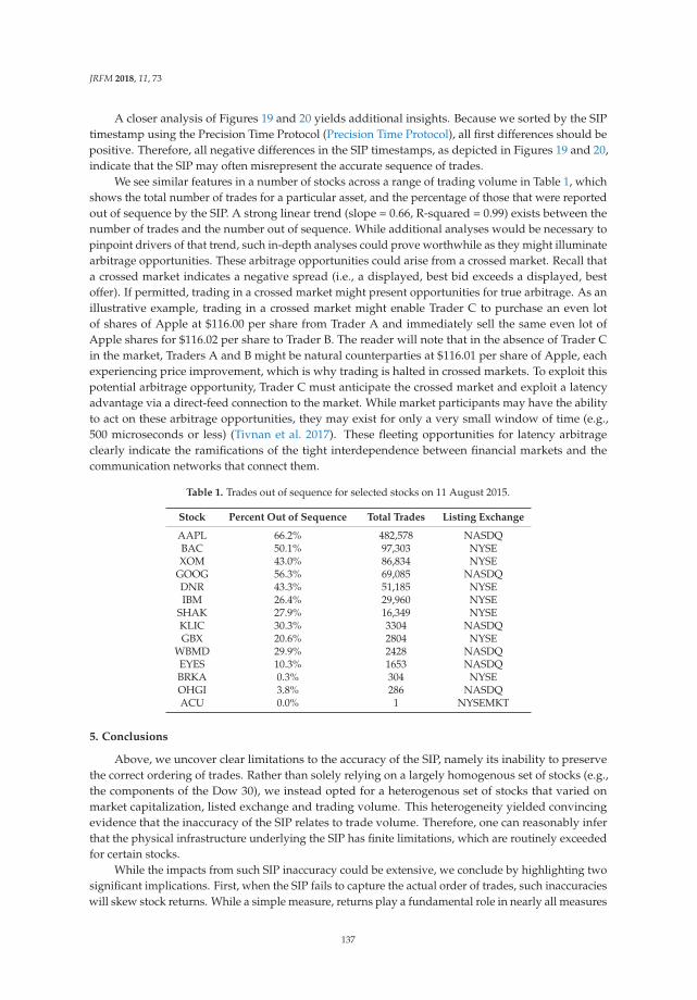
JRFM 2018, 11, 73
A closer analysis of Figures 19 and 20 yields additional insights. Because we sorted by the SIPtimestamp using the Precision Time Protocol (Precision Time Protocol), all first differences should bepositive. Therefore, all negative differences in the SIP timestamps, as depicted in Figures 19 and 20,indicate that the SIP may often misrepresent the accurate sequence of trades.
We see similar features in a number of stocks across a range of trading volume in Table 1, whichshows the total number of trades for a particular asset, and the percentage of those that were reportedout of sequence by the SIP. A strong linear trend (slope = 0.66, R-squared = 0.99) exists between thenumber of trades and the number out of sequence. While additional analyses would be necessary topinpoint drivers of that trend, such in-depth analyses could prove worthwhile as they might illuminatearbitrage opportunities. These arbitrage opportunities could arise from a crossed market. Recall thata crossed market indicates a negative spread (i.e., a displayed, best bid exceeds a displayed, bestoffer). If permitted, trading in a crossed market might present opportunities for true arbitrage. As anillustrative example, trading in a crossed market might enable Trader C to purchase an even lotof shares of Apple at $116.00 per share from Trader A and immediately sell the same even lot ofApple shares for $116.02 per share to Trader B. The reader will note that in the absence of Trader Cin the market, Traders A and B might be natural counterparties at $116.01 per share of Apple, eachexperiencing price improvement, which is why trading is halted in crossed markets. To exploit thispotential arbitrage opportunity, Trader C must anticipate the crossed market and exploit a latencyadvantage via a direct-feed connection to the market. While market participants may have the abilityto act on these arbitrage opportunities, they may exist for only a very small window of time (e.g.,500 microseconds or less) (Tivnan et al. 2017). These fleeting opportunities for latency arbitrageclearly indicate the ramifications of the tight interdependence between financial markets and thecommunication networks that connect them.
Table 1. Trades out of sequence for selected stocks on 11 August 2015.
Stock Percent Out of Sequence Total Trades Listing Exchange
AAPL 66.2% 482,578 NASDQBAC 50.1% 97,303 NYSEXOM 43.0% 86,834 NYSE
GOOG 56.3% 69,085 NASDQDNR 43.3% 51,185 NYSEIBM 26.4% 29,960 NYSE
SHAK 27.9% 16,349 NYSEKLIC 30.3% 3304 NASDQGBX 20.6% 2804 NYSE
WBMD 29.9% 2428 NASDQEYES 10.3% 1653 NASDQBRKA 0.3% 304 NYSEOHGI 3.8% 286 NASDQACU 0.0% 1 NYSEMKT
5. Conclusions
Above, we uncover clear limitations to the accuracy of the SIP, namely its inability to preservethe correct ordering of trades. Rather than solely relying on a largely homogenous set of stocks (e.g.,the components of the Dow 30), we instead opted for a heterogenous set of stocks that varied onmarket capitalization, listed exchange and trading volume. This heterogeneity yielded convincingevidence that the inaccuracy of the SIP relates to trade volume. Therefore, one can reasonably inferthat the physical infrastructure underlying the SIP has finite limitations, which are routinely exceededfor certain stocks.
While the impacts from such SIP inaccuracy could be extensive, we conclude by highlighting twosignificant implications. First, when the SIP fails to capture the actual order of trades, such inaccuracieswill skew stock returns. While a simple measure, returns play a fundamental role in nearly all measures
137
JRFM 2018, 11, 73
of risk; therefore, the inaccuracies of the SIP uncovered here could reveal extensive limitations for riskmanagement. Finally, given the preponderance of algorithmic trading in today’s U.S. equity markets,disordered trades and subsequently skewed returns could result in positive feedback driving marketsaway from efficient, price discovery.
While convincing, our findings on the accuracy of the SIP are not exhaustive, so we thereforeencourage researchers to consider additional dimensions of analysis for future research. A longitudinalstudy might address the accuracy of the SIP over time. Another study might compare the accuracy ofthe SIP for component stocks of prevailing market indices (e.g., Dow 30, S P 500 and Russell 3000).Lastly, we suggest that a direct extension of this study of the SIP accuracy of trades includes an analysisof updated quotes.
Author Contributions: Conceptualization, B.F.T. (Brian F. Tivnan), S.M.B., M.T.K.K., M.T.M., D.S., J.R.T., B.F.T.(Brendan F. Tivnan) and J.G.V.; Data curation, B.F.T. (Brian F. Tivnan), D.S., T.A.B.-H. and J.G.V.; Formal analysis,B.F.T. (Brian F. Tivnan), D.S., J.R.T. and M.T.K.K.; Funding acquisition, B.F.T. (Brian F. Tivnan) and S.M.B.;Investigation, M.T.K.K.; Methodology, B.F.T. (Brian F. Tivnan), D.S., J.R.T., Carl Burke, M.T.K.K., M.T.M. and J.G.V.;Project administration, B.F.T. (Brian F. Tivnan) and J.G.V.; Resources, B.F.T. (Brian F. Tivnan) and S.M.B.; Software,D.S., J.R.T., T.A.B.-H., Carl Burke, M.T.K.K. and M.T.M.; Supervision, B.F.T. (Brian F. Tivnan) and J.G.V.; Validation,B.F.T. (Brian F. Tivnan); Visualization, D.S., J.R.T., T.A.B.-H., Carl Burke, M.T.K.K. and B.F.T. (Brendan F. Tivnan);Writing—original draft, B.F.T. (Brian F. Tivnan) and J.G.V.; Writing—review & editing, B.F.T. (Brian F. Tivnan),B.F.T. (Brendan F. Tivnan) and J.G.V.
Funding: The researchers are grateful for external funding which supported the initial phase of this study. B.F.T.,D.S., J.R.T., T.A.B-H., C.D.B., S.M.B., M.T.T.K., M.T.M., and J.G.V. were supported by U.S. Department of HomelandSecurity award #HSHQDC-14-D-00006. The views, opinions and/or findings expressed are those of the authorsand should not be interpreted as representing the official views or policies of the Department of HomelandSecurity or the U.S. Government.
Acknowledgments: The authors gratefully acknowledge the following: Collaborative contributions from RichardBookstaber, Michael Foley, Christine Harvey, Eric Hunsader, Neil Johnson and Mark Paddrik; helpful insightsfrom Anshul Anand, Chris Danforth, David Dewhurst, Peter Dodds, Jordan Feidler, Andre Frank, Bill Gibson,Frank Hatheway, John Ring, Chuck Schnitzlein, Colin Van Oort, Tom Wilk and attendees at the 2016 InternationalCongress on Agent Computing. The authors’ affiliation with The MITRE Corporation is provided for identificationpurposes only and is not intended to convey or imply MITRE’s concurrence with, or support for, the positions,opinions or viewpoints expressed by the authors.
Conflicts of Interest: The authors declare no conflict of interest.
Appendix A
Table A1. Exchanges and Trade Reporting Facilities.
Exchange Family Exchange Name Abbreviations Geographic Location
BATS BATS BATS/BZX Secaucus, NJBATS-Y BATY/BYX Secaucus, NJ
Direct Edge A EDGA Secaucus, NJDirect Edge X EDGX Secaucus, NJ
Chicago Chicago Stock Exchange CHX Secaucus, NJNASDAQ NASDAQ NASD Carteret, NJ
NASDAQ-Boston NQBS Carteret, NJNASDAQ-Philadelphia NQPH Carteret, NJ
NYSE New York Stock Exchange NYSE Mahwah, NJNew York Stock Exchange—ARCA ARCA Mahwah, NJNew York Stock Exchange—Market AMEX/NY-MKT Mahwah, NJ
SIP NYSE Trade Reporting Facility NTRF Mahwah, NJSIP NASDAQ Trade Reporting Facility QTRF Carteret, NJ
References
Angel, James J. 2014. When Finance Meets Physics: The Impact of the Speed of Light on Financial Markets andTheir Regulation. Financial Review 49: 271–81. [CrossRef]
Arnuk, Salvatore, and Joseph Saluzzi. 2012. Broken Markets. Upper Saddle River, New Jersey: FT Press.
138

JRFM 2018, 11, 73
Bartlett, Robert P., and Justin McCrary. 2017. How Rigged Are Stock Markets?: Evidence from MicrosecondTimestamps. Available online: https://www.nber.org/papers/w22551 (accessed on 30 September 2018).
Bodek, Haim. 2013. The Problem of HFT: Collected Writings on High Frequency Trading & Stock Market StructureReform. Norwalk: Decimus Capital Markets.
Consolidated Tape Association. Available online: https://www.ctaplan.com/index (accessed on 30 September 2018).Cont, Rama. 2001. Empirical Properties of Asset Returns. Quantitative Finance 1: 223–36. [CrossRef]Ding, Shengwei, John Hanna, and Terrence Hendershott. 2014. How Slow is the NBBO? A Comparison with Direct
Exchange Feeds. Financial Review 49: 313–32.Johnson, Neil, Guannan Zhao, Eric Hunsader, Jing Meng, Amith Ravindar, Spencer Carran, and Brian Tivnan.
2012. Financial Black Swans Driven by Ultrafast, Machine Ecology. Available online: https://arxiv.org/abs/1202.1448 (accessed on 30 September 2018).
Johnson, Neil, Guannan Zhao, Eric Hunsader, Hong Qi, Nicholas Johnson, Jing Meng, and Brian Tivnan. 2013.Abrupt Rise of New Machine Ecology Beyond Human Response Time. Scientific Reports 3: 2627. [CrossRef][PubMed]
Lewis, Michael. 2014. Flash Boys: A Wall Street Revolt. New York: Norton & Company.Mandelbrot, Benoit. 1963. Variation of Certain Speculative Prices. New York: Springer.Nanex Research. 2014a. NBBO Misfiring. Available online: http://www.nanex.net/aqck2/4616.html (accessed on
30 September 2018).Nanex Research. 2014b. Perfect Pilfering. Available online: http://www.nanex.net/aqck2/4661.html (accessed on
30 September 2018).Patterson, Scott, and Jennifer Strasburg. 2012a. Traders Navigate a Murky New World. Wall Street Journal, April 9.Patterson, Scott. 2012b. Dark Pools. New York: Crown Pub.Precision Time Protocol is “a protocol used to synchronize clocks throughout a computer network”.
Available online: https://en.wikipedia.org/wiki/Precision_Time_Protocol (accessed on 30 September 2018).Securities and Exchange Commission. Regulation NMS. Available online: https://www.sec.gov/rules/final/34-
51808.pdf (accessed on 30 September 2018).Tivnan, Brian F., and Brendan F. Tivnan. 2016. Impacts of Market Liquidity and Heterogeneity in the Investor
Decision Cycle on the National Market System. Paper presented at SWARMFEST 2016: 20th Annual Meetingon Agent-Based Modeling & Simulation, Burlington, VT, USA, July 31–August 3.
Tivnan, Brian F., Matthew T. K. Koehler, David Slater, Jason Veneman, and Brendan F. Tivnan. 2017. Toward aModel of the U.S. Stock Market: How Important is the Securities Information Processor? Paper presented atthe 2017 Winter Simulation Conference, Las Vegas, NV, USA, 3–6 December; Piscataway, NJ, USA: Instituteof Electrical and Electronics Engineers, Inc., pp. 1181–92.
Unlisted Trading Privileges. Available online: http://www.utpplan.com/overview (accessed on 30 September 2018).
© 2018 by the authors. Licensee MDPI, Basel, Switzerland. This article is an open accessarticle distributed under the terms and conditions of the Creative Commons Attribution(CC BY) license (http://creativecommons.org/licenses/by/4.0/).
139
Journal of
Risk and FinancialManagement
Article
Expectations for Statistical Arbitrage in EnergyFutures Markets
Tadahiro Nakajima 1,2
1 The Kansai Electric Power Company, Incorporated, 6-16, Nakanoshima 3-chome, Kita-Ku, Osaka 530-8270,Japan; [email protected]; Tel.: +81-6-6441-8821
2 Graduate School of Economics, Kobe University, 2-1 Rokkodai-cho Nada-ku, Kobe 657-8501, Japan
Received: 7 December 2018; Accepted: 12 January 2019; Published: 15 January 2019
Abstract: Energy futures have become important as alternative investment assets to minimize thevolatility of portfolio return, owing to their low links with traditional financial markets. In order tomake energy futures markets grow further, it is necessary to expand expectations of returns fromtrading in energy futures markets. Therefore, this study examines whether profits can be earnedby statistical arbitrage between wholesale electricity futures and natural gas futures listed on theNew York Mercantile Exchange. On the assumption that power prices and natural gas prices have acointegration relationship, as tested and supported by previous studies, the short-term deviation fromthe long-term equilibrium is regarded as an arbitrage opportunity. The results of the spark-spreadtrading simulations using historical data from 2 January 2014 to 29 December 2017 show about 30%yield at maximum. This study shows the possibility of generating earnings in energy futures market.
Keywords: cointegration; statistical arbitrage; natural gas; wholesale electricity; futures market;spark spread
1. Introduction
A variety of energy derivatives are listed and actively traded on the New York MercantileExchange (NYMEX), the Intercontinental Exchange Futures, and other commodity exchanges.For example, Figure 1 traces the open interests of West Texas Intermediate (WTI) crude oil futuresand Henry Hub natural gas futures from the beginning of 1991 to the end of 2016. Both open interestswere temporarily stagnated owing to the Lehman shock that preceded the global financial crisis, but ingeneral, they have tended to increase.
Most energy companies in the supply chain of crude oil, natural gas, and power handle extremelylarge amounts of physical assets. Furthermore, they are exposed to large price fluctuations owing tothe geopolitical issues, demand from newly emerging countries, and resource nationalism. Moreover,power futures prices have a very complicated relationship with spot prices and usually contain largeforward risk premium, because electricity cannot be stored economically, unlike other commodities,as Haugom et al. (2014, 2018) point out. Therefore, these companies must positively trade energyderivatives in order to hedge their risks even slightly.
Institutional investors hold energy derivatives as alternative investment to benefit from portfoliodiversification, because these derivatives have a low correlation with conventional investment, such asstocks, bonds, and foreign currencies. Any entity in any country consumes energy resource, such ascrude oil, natural gas, and coal, although they cannot control the price fluctuation risks by themselves.Therefore, there are great expectations of energy derivatives, as most market participants aim tominimize the volatility of return on investment.
JRFM 2019, 12, 14; doi:10.3390/jrfm12010014 www.mdpi.com/journal/jrfm140
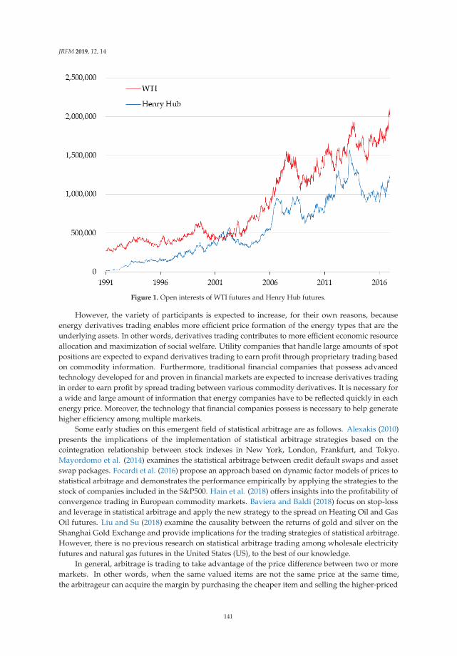
JRFM 2019, 12, 14
Figure 1. Open interests of WTI futures and Henry Hub futures.
However, the variety of participants is expected to increase, for their own reasons, becauseenergy derivatives trading enables more efficient price formation of the energy types that are theunderlying assets. In other words, derivatives trading contributes to more efficient economic resourceallocation and maximization of social welfare. Utility companies that handle large amounts of spotpositions are expected to expand derivatives trading to earn profit through proprietary trading basedon commodity information. Furthermore, traditional financial companies that possess advancedtechnology developed for and proven in financial markets are expected to increase derivatives tradingin order to earn profit by spread trading between various commodity derivatives. It is necessary fora wide and large amount of information that energy companies have to be reflected quickly in eachenergy price. Moreover, the technology that financial companies possess is necessary to help generatehigher efficiency among multiple markets.
Some early studies on this emergent field of statistical arbitrage are as follows. Alexakis (2010)presents the implications of the implementation of statistical arbitrage strategies based on thecointegration relationship between stock indexes in New York, London, Frankfurt, and Tokyo.Mayordomo et al. (2014) examines the statistical arbitrage between credit default swaps and assetswap packages. Focardi et al. (2016) propose an approach based on dynamic factor models of prices tostatistical arbitrage and demonstrates the performance empirically by applying the strategies to thestock of companies included in the S&P500. Hain et al. (2018) offers insights into the profitability ofconvergence trading in European commodity markets. Baviera and Baldi (2018) focus on stop-lossand leverage in statistical arbitrage and apply the new strategy to the spread on Heating Oil and GasOil futures. Liu and Su (2018) examine the causality between the returns of gold and silver on theShanghai Gold Exchange and provide implications for the trading strategies of statistical arbitrage.However, there is no previous research on statistical arbitrage trading among wholesale electricityfutures and natural gas futures in the United States (US), to the best of our knowledge.
In general, arbitrage is trading to take advantage of the price difference between two or moremarkets. In other words, when the same valued items are not the same price at the same time,the arbitrageur can acquire the margin by purchasing the cheaper item and selling the higher-priced
141

JRFM 2019, 12, 14
one. For instance, spatial arbitrage opportunities occur because gold futures is listed on commodityexchanges around the world and the price varies by exchanges. However, arbitrage opportunitiesin such similar securities cannot last long, because the price difference is adjusted by arbitrageursimmediately. As another example, statistical arbitrage is possible by taking advantage of the pricedifference between different securities. Statistical arbitrage is evaluated by quantitative methods. It isconditional on finding and estimating a statistical relationship between multiple securities.
Many previous studies accept the cointegration relationship between electricity prices and naturalgas prices. Serletis and Herbert (1999), Emery and Liu (2002), Serletis and Shahmoradi (2006),and Mjelde and Bessler (2009) accept that the regional wholesale electricity index is cointegratedwith the natural gas price index in North America. Asche et al. (2006), Joëts and Mignon (2011),Furió and Chuliá (2012), and Freitas and Silva (2015) indicate that there is a cointegration relationshipin Europe. Mohammadi (2009) accepts the cointegration hypothesis to examine the relationshipbetween retail power prices and gas prices at wellhead in the US. Gautam and Paudel (2018) examinethe demand for power in the residential, commercial, and industrial sectors after the acceptance ofcointegration with gas prices.
Therefore, unconditionally accepting the cointegration relationship between natural gas futuresprices and wholesale electricity futures prices, we investigate the possibility of profit acquisition inspark-spread trading by regarding the deviation from the long-run equilibrium between these twovariables as arbitrage opportunities. The results present profitability by statistical arbitrage tradingusing a very simple algorithm based on a long-term equilibrium formula between wholesale electricityfutures and natural gas futures.
The remainder of this paper is organized as follows. Section 2 explains the methodology adopted.Section 3 describes the data analyzed and used in the simulations. Section 4 presents the results of theanalyses and simulations. Section 5 provides a discussion about the results.
2. Methodology
When the cointegration hypothesis between natural gas futures prices and wholesale electricityfutures prices is accepted unconditionally, the possibility of earning profit by statistical arbitragebetween these two markets is confirmed.
We develop the algorithm under the following two hypotheses. First, long-term equilibriumbetween gas prices and power prices does not fluctuate dramatically over the short term. Second,these prices do not fully reflect each other on the day. Thereafter, we verify the profitability based onthe simulation using historical data.
2.1. Monitoring Prices
As a reference value for transaction candidate date, we monitor daily historical data for three yearsup to the day before that date. Specifically, we monitor the trend of non-stationarity of both economicvariables. We adopt the unit root test developed by Kwiatkowski et al. (1992), the so-called KPSStest. Because the KPSS test, which has a null hypothesis of a stationary, is adequate for monitoringthe trend of non-stationarity, while these variables are predicted to have a unit root like the othermarket variables. Moreover, we examine the stationarity of these variables and the stationarity ofthe first differences of these variables for the whole period by the augmented Dickey–Fuller (ADF)test and Phillips and Perron (1988) PP test. In addition, we monitor the tendency of the relationshipbetween these prices by the cointegration test proposed by Johansen (1988). We unconditionallyaccept the cointegration hypothesis between wholesale power futures prices and natural gas futuresprices supported by past literature to develop the trading algorithm. Therefore, even if the stationaryhypothesis is accepted or the cointegration hypothesis rejected, the cointegration relationship is notdenied simply by regarding the results as a power shortage caused by the number of samples or thetest methodology. However, to respect the price trend, we attempt to reflect these test results in thetrading strategy.
142

JRFM 2019, 12, 14
2.2. Estimation of Long-Term Equilibrium Equations
The long-term equilibrium equation estimated at trading candidate date t is
E(t) = α(t) × G(t) + β(t) (1)
where E(t) and G(t) are futures prices of wholesale electricity and natural gas, respectively; and α(t) andβ(t) are coefficients estimated by dynamic ordinary least squares (DOLS) using three years up to theday before date t as the sample period. When we estimate the cointegrating vector using DOLS, it isacceptable to determine the orders of lead and lag by minimizing the information criterion. However,the lead values cannot be utilized in a real trading strategy, because these are prices after the tradingcandidate date. Therefore, the cointegrating vectors are obtained by ordinary least squares estimationof the coefficients of the equation
E(t) = α(t) × G(t) + β(t) + γ(t) × (G(t) − G(t − 1)) (2)
The sampling period is from t − 3 × 365 to t − 1, and therefore, we do not use prices after thetransaction candidate date.
2.3. Trading
As with ordinary spread trading, this study combines both a long and short position at the sametime in gas and power as related futures contracts. In other words, when the price difference is widerthan the appropriate level, we sell higher-priced futures and buy lower-priced futures. On the contrary,when the price difference is narrower than the appropriate level, we buy the higher-priced futures andsell the lower-priced futures. The decision on whether the price difference between gas futures andelectricity futures is appropriate depends on Equation (1).
The specific procedure is as follows. When
E(t) > α(t) × G(t) + β(t) (3)
the electricity price is considered high and the gas price low. Therefore, we settle the long position inelectricity and take a short position in electricity for
E(t)/(E(t) + G(t)) (4)
Moreover, we take a long position in gas for
G(t)/(E(t) + G(t)) (5)
Conversely, whenE(t) < α(t) × G(t) + β(t) (6)
the electricity price is considered low and the gas price is high. Therefore, we settle the long positionin gas and take a short position in gas for
G(t)/(E(t) + G(t)) (7)
Moreover, we take a long position in electricity for
E(t)/(E(t) + G(t)) (8)
143
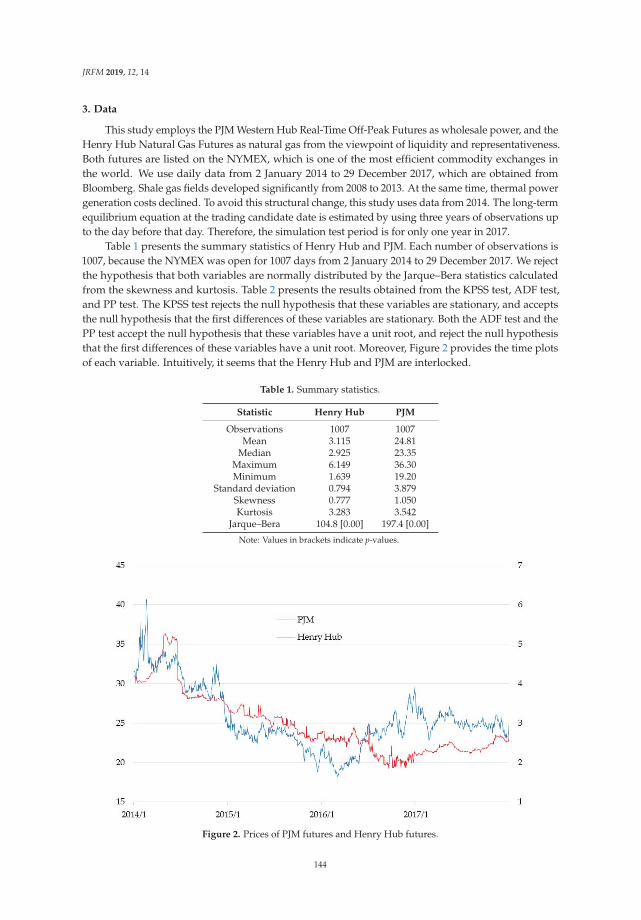
JRFM 2019, 12, 14
3. Data
This study employs the PJM Western Hub Real-Time Off-Peak Futures as wholesale power, and theHenry Hub Natural Gas Futures as natural gas from the viewpoint of liquidity and representativeness.Both futures are listed on the NYMEX, which is one of the most efficient commodity exchanges inthe world. We use daily data from 2 January 2014 to 29 December 2017, which are obtained fromBloomberg. Shale gas fields developed significantly from 2008 to 2013. At the same time, thermal powergeneration costs declined. To avoid this structural change, this study uses data from 2014. The long-termequilibrium equation at the trading candidate date is estimated by using three years of observations upto the day before that day. Therefore, the simulation test period is for only one year in 2017.
Table 1 presents the summary statistics of Henry Hub and PJM. Each number of observations is1007, because the NYMEX was open for 1007 days from 2 January 2014 to 29 December 2017. We rejectthe hypothesis that both variables are normally distributed by the Jarque–Bera statistics calculatedfrom the skewness and kurtosis. Table 2 presents the results obtained from the KPSS test, ADF test,and PP test. The KPSS test rejects the null hypothesis that these variables are stationary, and acceptsthe null hypothesis that the first differences of these variables are stationary. Both the ADF test and thePP test accept the null hypothesis that these variables have a unit root, and reject the null hypothesisthat the first differences of these variables have a unit root. Moreover, Figure 2 provides the time plotsof each variable. Intuitively, it seems that the Henry Hub and PJM are interlocked.
Table 1. Summary statistics.
Statistic Henry Hub PJM
Observations 1007 1007Mean 3.115 24.81
Median 2.925 23.35Maximum 6.149 36.30Minimum 1.639 19.20
Standard deviation 0.794 3.879Skewness 0.777 1.050Kurtosis 3.283 3.542
Jarque–Bera 104.8 [0.00] 197.4 [0.00]
Note: Values in brackets indicate p-values.
Figure 2. Prices of PJM futures and Henry Hub futures.
144
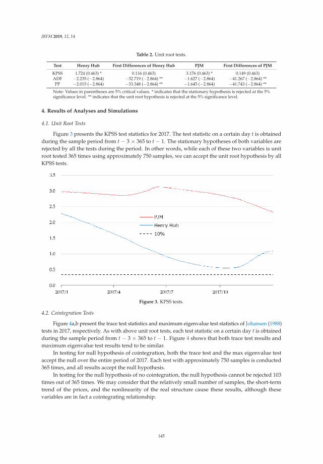
JRFM 2019, 12, 14
Table 2. Unit root tests.
Test Henry Hub First Differences of Henry Hub PJM First Differences of PJM
KPSS 1.724 (0.463) * 0.116 (0.463) 3.176 (0.463) * 0.149 (0.463)ADF −2.235 (−2.864) −32.719 (−2.864) ** −1.627 (−2.864) −41.267 (−2.864) **PP −2.015 (−2.864) −33.348 (−2.864) ** −1.645 (−2.864) −41.743 (−2.864) **
Note: Values in parentheses are 5% critical values. * indicates that the stationary hypothesis is rejected at the 5%significance level. ** indicates that the unit root hypothesis is rejected at the 5% significance level.
4. Results of Analyses and Simulations
4.1. Unit Root Tests
Figure 3 presents the KPSS test statistics for 2017. The test statistic on a certain day t is obtainedduring the sample period from t − 3 × 365 to t − 1. The stationary hypotheses of both variables arerejected by all the tests during the period. In other words, while each of these two variables is unitroot tested 365 times using approximately 750 samples, we can accept the unit root hypothesis by allKPSS tests.
Figure 3. KPSS tests.
4.2. Cointegration Tests
Figure 4a,b present the trace test statistics and maximum eigenvalue test statistics of Johansen (1988)tests in 2017, respectively. As with above unit root tests, each test statistic on a certain day t is obtainedduring the sample period from t − 3 × 365 to t − 1. Figure 4 shows that both trace test results andmaximum eigenvalue test results tend to be similar.
In testing for null hypothesis of cointegration, both the trace test and the max eigenvalue testaccept the null over the entire period of 2017. Each test with approximately 750 samples is conducted365 times, and all results accept the null hypothesis.
In testing for the null hypothesis of no cointegration, the null hypothesis cannot be rejected 103times out of 365 times. We may consider that the relatively small number of samples, the short-termtrend of the prices, and the nonlinearity of the real structure cause these results, although thesevariables are in fact a cointegrating relationship.
145

JRFM 2019, 12, 14
(a) Trace tests
(b) Max eigenvalue tests
Figure 4. Johansen tests.
4.3. Selection of Trading Dates
The selection of the trading dates depends on the test results related to the relationship betweenboth variables.
First, we define the period when the null hypothesis of no cointegration is rejected by theJohansen (1988) test as period A, and the period that is accepted as period B. Next, the three strategiesfor trading only in period A, only in period B, and in both periods are defined as conservative,aggressive, and neutral types, respectively. Finally, we simulate these three trading strategies andexamine their impact on profitability.
146
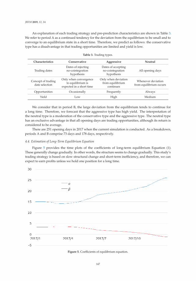
JRFM 2019, 12, 14
An explanation of each trading strategy and pre-prediction characteristics are shown in Table 3.We refer to period A as a continued tendency for the deviation from the equilibrium to be small and toconverge to an equilibrium state in a short time. Therefore, we predict as follows: the conservativetype has a disadvantage in that trading opportunities are limited and yield is low.
Table 3. Trading types.
Characteristics Conservative Aggressive Neutral
Trading datesDates of rejectingno-cointegration
hypothesis
Dates of acceptingno-cointegration
hypothesisAll opening days
Concept of tradingdate selection
Only when convergenceto equilibrium is
expected in a short time
Only when deviationfrom equilibrium
continues
Whenever deviationfrom equilibrium occurs
Opportunities Occasionally Frequently Always
Yield Low High Medium
We consider that in period B, the large deviation from the equilibrium tends to continue fora long time. Therefore, we forecast that the aggressive type has high yield. The interpretation ofthe neutral type is a moderation of the conservative type and the aggressive type. The neutral typehas an exclusive advantage in that all opening days are trading opportunities, although its return isconsidered to be average.
There are 251 opening days in 2017 when the current simulation is conducted. As a breakdown,periods A and B comprise 73 days and 178 days, respectively.
4.4. Estimation of Long-Term Equilibrium Equation
Figure 5 provides the time plots of the coefficients of long-term equilibrium Equation (1).These generally change gradually. In other words, the structure seems to change gradually. This study’strading strategy is based on slow structural change and short-term inefficiency, and therefore, we canexpect to earn profits unless we hold one position for a long time.
Figure 5. Coefficients of equilibrium equation.
147
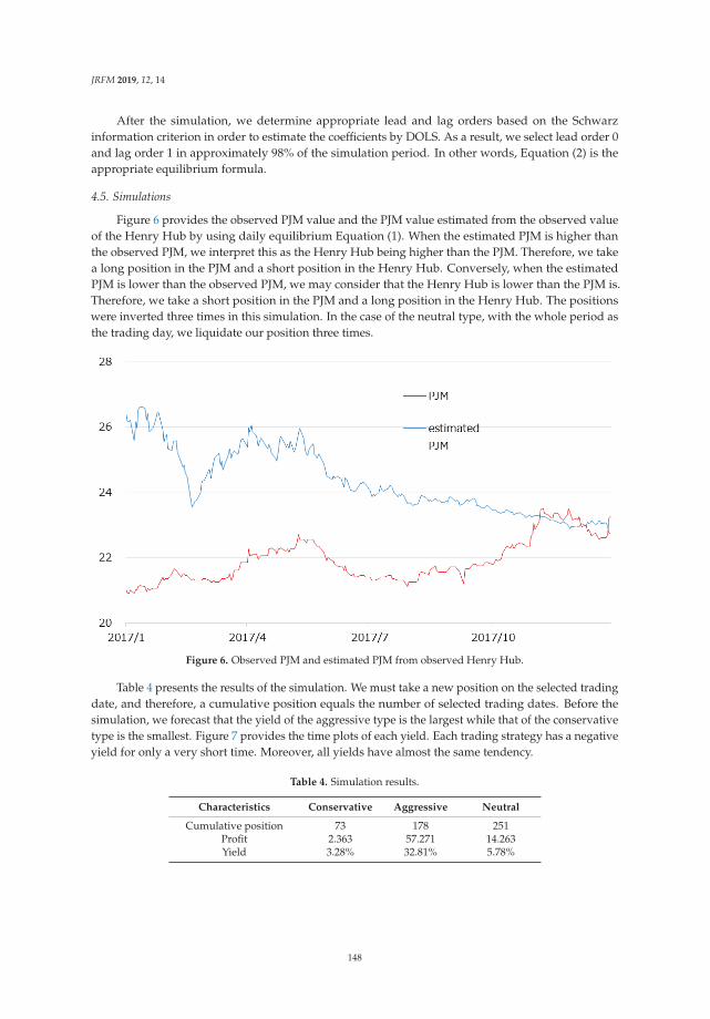
JRFM 2019, 12, 14
After the simulation, we determine appropriate lead and lag orders based on the Schwarzinformation criterion in order to estimate the coefficients by DOLS. As a result, we select lead order 0and lag order 1 in approximately 98% of the simulation period. In other words, Equation (2) is theappropriate equilibrium formula.
4.5. Simulations
Figure 6 provides the observed PJM value and the PJM value estimated from the observed valueof the Henry Hub by using daily equilibrium Equation (1). When the estimated PJM is higher thanthe observed PJM, we interpret this as the Henry Hub being higher than the PJM. Therefore, we takea long position in the PJM and a short position in the Henry Hub. Conversely, when the estimatedPJM is lower than the observed PJM, we may consider that the Henry Hub is lower than the PJM is.Therefore, we take a short position in the PJM and a long position in the Henry Hub. The positionswere inverted three times in this simulation. In the case of the neutral type, with the whole period asthe trading day, we liquidate our position three times.
Figure 6. Observed PJM and estimated PJM from observed Henry Hub.
Table 4 presents the results of the simulation. We must take a new position on the selected tradingdate, and therefore, a cumulative position equals the number of selected trading dates. Before thesimulation, we forecast that the yield of the aggressive type is the largest while that of the conservativetype is the smallest. Figure 7 provides the time plots of each yield. Each trading strategy has a negativeyield for only a very short time. Moreover, all yields have almost the same tendency.
Table 4. Simulation results.
Characteristics Conservative Aggressive Neutral
Cumulative position 73 178 251Profit 2.363 57.271 14.263Yield 3.28% 32.81% 5.78%
148
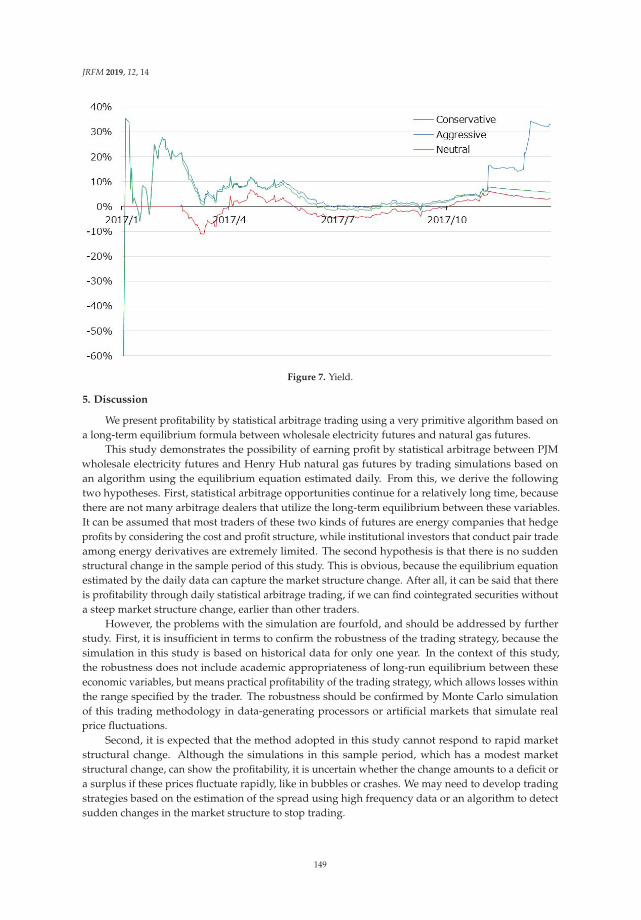
JRFM 2019, 12, 14
Figure 7. Yield.
5. Discussion
We present profitability by statistical arbitrage trading using a very primitive algorithm based ona long-term equilibrium formula between wholesale electricity futures and natural gas futures.
This study demonstrates the possibility of earning profit by statistical arbitrage between PJMwholesale electricity futures and Henry Hub natural gas futures by trading simulations based onan algorithm using the equilibrium equation estimated daily. From this, we derive the followingtwo hypotheses. First, statistical arbitrage opportunities continue for a relatively long time, becausethere are not many arbitrage dealers that utilize the long-term equilibrium between these variables.It can be assumed that most traders of these two kinds of futures are energy companies that hedgeprofits by considering the cost and profit structure, while institutional investors that conduct pair tradeamong energy derivatives are extremely limited. The second hypothesis is that there is no suddenstructural change in the sample period of this study. This is obvious, because the equilibrium equationestimated by the daily data can capture the market structure change. After all, it can be said that thereis profitability through daily statistical arbitrage trading, if we can find cointegrated securities withouta steep market structure change, earlier than other traders.
However, the problems with the simulation are fourfold, and should be addressed by furtherstudy. First, it is insufficient in terms to confirm the robustness of the trading strategy, because thesimulation in this study is based on historical data for only one year. In the context of this study,the robustness does not include academic appropriateness of long-run equilibrium between theseeconomic variables, but means practical profitability of the trading strategy, which allows losses withinthe range specified by the trader. The robustness should be confirmed by Monte Carlo simulationof this trading methodology in data-generating processors or artificial markets that simulate realprice fluctuations.
Second, it is expected that the method adopted in this study cannot respond to rapid marketstructural change. Although the simulations in this sample period, which has a modest marketstructural change, can show the profitability, it is uncertain whether the change amounts to a deficit ora surplus if these prices fluctuate rapidly, like in bubbles or crashes. We may need to develop tradingstrategies based on the estimation of the spread using high frequency data or an algorithm to detectsudden changes in the market structure to stop trading.
149

JRFM 2019, 12, 14
Third, although three kinds of algorithms are tested, these algorithms cannot maximize thereturns. The trading strategy for the maximization of returns under appropriate risk managementshould be able to be developed by changing the sample period to estimate the long-term equilibriumand the position depending on deviation from the long-term equilibrium. This study adopts estimationof long-term equilibrium formula over three years and daily trading with fixed size.
Finally, this study does not consider the constraints of actual exchange at all. In other words,this study assumes the unrealistic conditions in which the contract units are not restricted and tradingis possible at the prices of the historical data. Each exchange standardizes the contract specificationsfor each commodity, and therefore, we cannot adjust the contract units depending on the prices.Furthermore, actual transactions need transaction costs. It is impossible to avoid changing pricesowing to own orders. Buying causes price increases, and selling causes price drops. Apart from this,real transactions need real cash, including trading fees. Moreover, this study assumes that traders canconstantly and permanently increase their positions. In other words, they can take their positions,which need their infinite credit. These are impossible conditions for risk management.
These realistic tasks on commodity futures trading are unavoidable for practitioners, but tend tobe avoided academically. We hope that further study of commodity markets will be promoted fromvarious academic viewpoints.
Funding: This research received no external funding.
Acknowledgments: The author would like to thank Editage (www.editage.jp) for English language editing,and the anonymous reviewers, whose valuable comments helped to improve an earlier version of this paper.
Conflicts of Interest: The author declares no conflict of interest.
References
Alexakis, Christos. 2010. Long-run relations among equity indices under different market conditions: Implicationson the implementation of statistical arbitrage strategies. Journal of International Financial Markets, Institutionsand Money 20: 389–403. [CrossRef]
Asche, Frank, Petter Osmundsen, and Maria Sandsmark. 2006. The UK market for natural gas, oil and electricity:Are the prices decoupled? The Energy Journal 27: 27–40. [CrossRef]
Baviera, Raviera, and Tommaso Santagostino Baldi. 2018. Stop-loss and leverage in optimal statistical arbitragewith an application to energy market. Energy Economics. forthcoming. [CrossRef]
Emery, Gary W., and Qingfeng Wilson Liu. 2002. An analysis of the relationship between electricity and natural-gasfutures prices. The Journal of Futures Markets 22: 95–122. [CrossRef]
Focardi, Sergio M., Frank J. Fabozzi, and Ivan K. Mitov. 2016. A new approach to statistical arbitrage: Strategiesbased on dynamic factor models of prices and their performance. Journal of Banking & Finance 65: 134–55.[CrossRef]
Freitas, Carlos J. Pereira, and Patrícia Pereira da Silva. 2015. European Union emissions trading scheme impacton the Spanish electricity price during phase II and phase III implementation. Utilities Policy 33: 54–62.[CrossRef]
Furió, Dolores, and Helena Chuliá. 2012. Price and volatility dynamics between electricity and fuel costs: Someevidence for Spain. Energy Economics 34: 2058–65. [CrossRef]
Gautam, Tej K., and Krishna P. Paudel. 2018. Estimating sectoral demands for electricity using the pooled meangroup method. Applied Energy 231: 54–67. [CrossRef]
Hain, Martin, Julian Hess, and Marliese Uhrig-Homburg. 2018. Relative value arbitrage in European commoditymarkets. Energy Economics 69: 140–54. [CrossRef]
Haugom, Erik, Guttorm A. Hoff, Peter Molnár, Maria Mortensen, and Sjur Westgaard. 2014. The forecastingpower of medium-term futures contracts. Journal of Energy Markets 7: 1–23. [CrossRef]
Haugom, Erik, Guttorm A. Hoff, Peter Molnár, Maria Mortensen, and Sjur Westgaard. 2018. The forward premiumin the Nord Pool Power market. Emerging Markets Finance and Trade 54: 1793–807. [CrossRef]
Joëts, Marc, and Valérie Mignon. 2011. On the link between forward energy prices: A nonlinear panel cointegrationapproach. Energy Economics 34: 1170–75. [CrossRef]
150

JRFM 2019, 12, 14
Johansen, Søren. 1988. Statistical analysis of cointegration vectors. Journal of Economic Dynamics and Control12: 231–54. [CrossRef]
Kwiatkowski, Denis, Peter C. B. Phillips, Peter Schmidt, and Yongcheol Shin. 1992. Testing the null hypothesis ofstationarity against the alternative of a unit root. Journal of Econometrics 54: 159–78. [CrossRef]
Liu, Guo-Dong, and Chi-Wei Su. 2018. The dynamic causality between gold and silver prices in China market:A rolling window bootstrap approach. Finance Research Letters. forthcoming. [CrossRef]
Mayordomo, Sergio, Juan Ignacio Peña, and Juan Romo. 2014. Testing for statistical arbitrage in credit derivativesmarkets. Journal of Empirical Finance 26: 59–75. [CrossRef]
Mjelde, James W., and David A. Bessler. 2009. Market integration among electricity markets and their major fuelsource markets. Energy Economics 31: 482–91. [CrossRef]
Mohammadi, Hassan. 2009. Electricity prices and fuel costs: Long-run relations and short-run dynamics.Energy Economics 31: 503–9. [CrossRef]
Phillips, Peter C., and Pierre Perron. 1988. Testing for a unit root in time series regression. Biometrika 75: 335–46.[CrossRef]
Serletis, Apostolos, and John Herbert. 1999. The message in North American energy prices. Energy Economics21: 471–83. [CrossRef]
Serletis, Apostolos, and Akbar Shahmoradi. 2006. Measuring and testing natural gas and electricity marketsvolatility: Evidence from Alberta’s deregulated markets. Studies in Nonlinear Dynamics & Econometrics10: 1341. [CrossRef]
© 2019 by the author. Licensee MDPI, Basel, Switzerland. This article is an open accessarticle distributed under the terms and conditions of the Creative Commons Attribution(CC BY) license (http://creativecommons.org/licenses/by/4.0/).
151
Journal of
Risk and FinancialManagement
Article
Clarifying the Response of Gold Return to FinancialIndicators: An Empirical Comparative AnalysisUsing Ordinary Least Squares, Robust andQuantile Regressions
Takashi Miyazaki
Japan Center for Economic Research, 1-3-7, Otemachi, Chiyoda-ku, Tokyo 100-8066, Japan;[email protected]
Received: 17 December 2018; Accepted: 7 February 2019; Published: 14 February 2019
Abstract: In this study, I apply a quantile regression model to investigate how gold returns respond tochanges in various financial indicators. The model quantifies the asymmetric response of gold returnin the tails of the distribution based on weekly data over the past 30 years. I conducted a statisticaltest that allows for multiple structural changes and find that the relationship between gold returnand some key financial indicators changed three times throughout the sample period. According tomy empirical analysis of the whole sample period, I find that: (1) the gold return rises significantlyif stock returns fall sharply; (2) it rises as the stock market volatility increases; (3) it also rises whengeneral financial market conditions tighten; (4) gold and crude oil prices generally move towardthe same direction; and (5) gold and the US dollar have an almost constant negative correlation.Looking at each sample period, (1) and (2) are remarkable in the period covering the global financialcrisis (GFC), suggesting that investors divested from stocks as a risky asset. On the other hand, (3) isa phenomenon observed during the sample period after the GFC, suggesting that it reflects investors’behavior of flight to quality.
Keywords: gold return; asymmetric dependence; financial market stress; robust regression; quantileregression; structural break; flight to quality
JEL Classification: C12; C21; G11; G15; Q02
1. Introduction
Correlations across different asset classes increased during the global financial crisis (GFC) of2007–2009, and diversification effects did not work when most needed. With the financializationof commodities from the first half to the middle of the 2000s as cross-market linkages increased,many commodity prices plunged along with the stock market crash.1 This experience makes usrecognize the importance of accurately grasping the linkages or contagion between different assetclasses, and promote studies that unravel the transmission mechanism and spillover effect betweendifferent asset markets (see, e.g., Chudik and Fratzscher 2011; Diebold and Yilmaz 2012; Ehrmann et al.2011; Guo et al. 2011; Longstaff 2010).
Gold is generally seen as distinct from other traditional assets due to its special character. It isoften regarded as a safe haven, especially hedging against the downside risk of stocks or in times of
1 Previous studies that analyze the financialization of commodities and its background include Basu and Gavin (2011);Cheng and Xiong (2014); Domanski and Heath (2007); Silvennoinen and Thorp (2013); Tang and Xiong (2012).
JRFM 2019, 12, 33; doi:10.3390/jrfm12010033 www.mdpi.com/journal/jrfm152

JRFM 2019, 12, 33
financial turbulence. Academic research on gold as an investment asset has been increasing in recentyears (see, for example, O’Connor et al. 2015).
Existing literature that analyze the aspects of gold as a hedge or safety instrument compared withtraditional assets include Baur (2011); Baur and Lucey (2010); Baur and McDermott (2010); Cohenand Qadan (2010); Hillier et al. (2006); Hood and Malik (2013); Miyazaki et al. (2012); Miyazaki andHamori (2013, 2014, 2016, 2018); Piplack and Straetmans (2010); Qadan and Yagil (2012); World GoldCouncil (2010).
Baur (2011) analyzes the characteristics of gold based on multiple regression. He finds that goldhas a hedging function against US dollar depreciation but not against inflation as represented byconsumer prices. In addition, he argues that the role of gold as a safety asset is a phenomenon seen morerecently. Piplack and Straetmans (2010) examined the tail dependence between US stocks, governmentbonds, Treasury bills, and gold using the extreme value theory, and conducted statistical tests for flightto quality or flight to liquidity hypotheses. Their empirical results show that gold is, to some extent,effective as a safe asset against the plunge in the values of other assets. Furthermore, there are manyexisting studies that analyze the properties of commodities including gold as an investment vehicle(e.g., Akram 2009; Batten et al. 2010, 2014; Bhar and Hammoudeh 2011; Chan et al. 2011; Chevallierand Ielpo 2013; Ciner et al. 2013; Erb and Harvey 2006; Gorton and Rouwenhorst 2006; Hammoudehet al. 2009; Mensi et al. 2013; Sari et al. 2010; Silvennoinen and Thorp 2013, among others). In additionto these studies, Alkhatib and Harasheh (2018); Balcilar et al. (2018); Raza et al. (2018) covers up tomore recent sample period during and after the Brexit.
In this study, I use robust and quantile regression techniques to investigate how gold returnresponds to the changes in various financial indicators, specifically stock return, stock return volatility,financial market stress, crude oil, and the value of the US dollar. In the finance literature involvingempirical analyses, there are also many cases where interest is on the tails of the distribution ratherthan the average (expected value). Quantile regression introduced by Koenker and Bassett (1978)allows us to clarify the relationships between dependent variables and independent variables in thetails of the distributions of data that cannot be captured by only the expected value. Therefore, in recentyears in the field of economics and finance, econometricians have come to frequently use quantileregression making it one of the standard tools. Quantile regression is suitable for the purpose of thisstudy in quantifying the role of gold as a hedging function or safety asset.2 Empirical research usingquantile regression include Baur (2013); Baur and Schulze (2005); Bouoiyour et al. (2018); Mensi etal. (2014); Reboredo and Uddin (2016); Reboredo and Uddin (2016) applied quantile regression toanalyze the impact of financial stress and policy uncertainty in the US on a wide range of commodityfutures prices.
This paper clarifies the role or characteristics of gold as an investment asset, on which, so far,academic research has been relatively scarce in the finance literature. Similar to the motivation ofReboredo and Uddin (2016), this study is also interested in the way gold return responds to a surgein financial market stress, sharp drop in stock prices, and stock market volatility. One novelty of thisstudy is that it considers multiple structural breaks that are endogenously determined. Our empiricalresults show that the relationship between gold and financial variables mentioned above is not stableand have experienced several structural changes over time. In addition, we provide evidence thatgold return rises in response to a plunge in stock prices and a rapid rise in stress in the financialmarkets, suggesting the role of gold as a safe haven. This result tells us that investors are takinga “flight-to-quality” behavior.
The rest of the paper is organized as follows. In the next section, we briefly outline econometricmethodologies used in this paper comprising robust and quantile regression techniques. In addition
2 One of the other ways to disentangle the interdependence of data in the tails of the distribution is a method using extremevalue theory. Related research includes Hartmann et al. (2004); Piplack and Straetmans (2010); Straetmans et al. (2008).
153
JRFM 2019, 12, 33
to presenting data for the analysis, we construct the indicators to measure the level of stress in thefinancial markets in Section 3. Section 4 presents our major empirical results, while Section 5 concludes.
2. Econometric Methodology
In this section, we outline the robust and quantile regression techniques to be used in this study.While both regression techniques address outliers in the data and asymmetry of distributions, theirconcepts and approaches are considerably different.
2.1. Robust Regression
The property of an ordinary least squares (OLS) estimator being BLUE (Best Linear UnbiasedEstimator) depends on the assumption about the error term. Robust regression is an estimation methodfor correcting the bias of the OLS estimator caused by the existence of outliers and heteroskedasticity.OLS places equal weights to all observations, whereas robust regression reduces the weights on outliersto mitigate the latter’s influence. Robust regression is insensitive to small changes in the sample anddistributional assumptions of the data. It is also useful in separating the contribution of the part of thedata near the average and the part in the tails.3
Among the different variations of weight functions, I choose Bisquare defined as follows.⎧⎪⎨⎪⎩c2
6
(1 −(
1 −(
Xc
)2)3)
, if |X| ≤ c,
c2
6 , otherwise,
(1)
where c is an arbitrary positive tuning constant set to c = 4.685 in Bisquare form.4
2.2. Quantile Regression
Quantile regression is a method of modeling and estimating the relationship between a dependentvariable and independent variables in the tails of the distribution (more specifically, quantile).5
The distribution of returns of financial assets frequently exhibits the statistical property of heavy tails(see, for example, Cont 2001). If heavy tails and/or asymmetry in the distributions exist, the assumptionof normality is not satisfied. Therefore, inference based on classical regression models may leadto misleading conclusions. By utilizing quantile regression, researchers can reveal more accuratedependence structure between variables according to market conditions such as bull or bear markets,and completely know the distribution of returns.
OLS minimizes the sum of squared residuals,
minα,β
T
∑t=1
(yt − α − βxt)2 (2)
whereas quantile regression minimizes the following loss function,
minα(τ),β(τ)
T
∑t=1
ρτ(yt − α(τ)− β(τ)xt) (3)
3 See Chapter 8 of Fabozzi et al. (2014).4 EViews 9.5 is used for the robust regression in this study. For a more detailed technical description, refer to pp. 405-424 in
IHS Global Inc. (2016).5 For a succinct explanation of quantile regression, I recommend Koenker and Hallock (2001) and Rodriguez and Yao (2017).
For more formal treatments, refer to textbooks such as Chapter II.7.2 of Alexander (2008), Chapter 7 of Fabozzi et al. (2014);Hao and Naiman (2007). For nonparametric approach of the quantile regression, see Chao et al. (2012); Franke et al. (2015).
154

JRFM 2019, 12, 33
where ρτ(u) is the check function defined as follows.
ρτ(u) = u(τ − 1{u ≤ 0}) ={−(1 − τ)u, u ≤ 0
τu, u > 0(4)
where u = yt − α(τ)− β(τ)xt, and τ ∈ (0, 1) indicates the level of quantile. In particular, if τ = 0.5,that is the median, the quantile regression corresponds to the least absolute deviation method.
In summary, the techniques of robust regression and quantile regression model and estimate therelationships between the dependent variable and independent variables in the center of and in thetails of data distribution, respectively. Resorting to these two regression methods, we can closely shedlight on the characteristics of gold return than in previous literature.
3. Data
We adopt the US as a reference market affecting gold price. The US still possesses a dominantinfluence in the global financial markets, and plays the most important role to transmit financial shocks(see, e.g., Chudik and Fratzscher 2011; Ehrmann et al. 2011). In this study, we focus on the relationshipsbetween gold and a variety of financial indicators, specifically stock market return, stock marketreturn volatility, crude oil, the value of the US dollar against major currencies, and general financialmarket conditions in the US.6 The sample period covers about past three decades of weekly data from5 January 1990 to 27 April 2018. Weekly frequency seems to be an appropriate choice to ensure thenumber of samples and eliminate noise that can occur in daily data. Table 1 displays the data sources.All three financial instruments, namely gold, S&P 500 index and crude oil are spot prices.
Table 1. Data sources.
Variable Source
Gold price, PM fix(spot) Bloomberg; originally provided by London Bullion Market Association (LBMA)
S&P 500 Index(spot) Bloomberg; originally provided by S&P Dow Jones Indices
TED spread Federal Reserve Economic Database (FRED) of St. Louis Fed
Aaa-10Y spread Federal Reserve Economic Database (FRED) of St. Louis Fed
Baa-Aaa spread Federal Reserve Economic Database (FRED) of St. Louis Fed
West Texas Intermediate (WTI)(spot)
Federal Reserve Economic Database (FRED) of St. Louis Fed; originallyprovided by US Energy Information Administration (EIA)
Trade Weighted US Dollar Index: Major Currencies Federal Reserve Economic Database (FRED) of St. Louis Fed; originallyprovided by Board of Governors of the Federal Reserve System (US)
3.1. Measure of Financial Market Stress
Several variables could serve as indicators of financial market conditions. To construct an indexto measure the stress level of financial markets, we employ principal component analysis (PCA).Specifically, we apply PCA to the following four interest rate-related variables; Treasury-EuroDollar(TED) spread,7 credit spread,8 default spread,9 and term spread,10 and set the extracted principal
6 We recognize its relevance, but exclude bond from our analysis since we consider that information in bond market isincluded, to some extent, in the financial market stress index constructed below. Existing studies explicitly demonstratingthe connection of gold with bond include Agyei-Ampomah et al. (2014); Baur and Lucey (2010); Baur and McDermott (2010);Ciner et al. (2013); Miyazaki and Hamori (2016); Piplack and Straetmans (2010).
7 TED spread is calculated as the spread between the three-month London interbank offered rate based on US dollars and thethree-month Treasury bill rate.
8 Credit spread is calculated as the yield spread between Baa- and Aaa-ranked corporate bonds.9 Default spread is calculated as the yield spread between Aaa-ranked corporate bonds and Treasuries with 10-year
constant maturities.10 Term spread is calculated as the yield spread between Treasuries of 10-year and three-month constant maturities.
155

JRFM 2019, 12, 33
components as a measure for the degree of financial market stress.11 These financial indicators actas liquidity risk, credit risk, default risk, and monetary policy stance or recession risk,12 respectively.Table 2 reports the results of PCA extracted from the four risk indicators above, and Figure 1 illustratestheir evolution. According to Table 2, factor loadings of all financial risk indicators are positive forthe first principal component. As seen in Figure 1, the first principal component experiences spikesin the financial turmoil episodes such as failure of long-term capital management (LTCM), dot-combubble collapse, and Lehman Brothers bankruptcy. From these observational findings, we interpret thefirst principal component as the degree of general financial market stress and use it as an indicator tomeasure the tightness of the financial market in the following empirical analysis.
Table 2. Principal component analysis: financial market stress.
Factor Loadings
1st 2nd 3rd 4th
TED 0.088 0.796 0.354 0.483Aaa-10Y 0.628 −0.068 −0.626 0.458Baa-Aaa 0.627 0.324 0.079 −0.704TERM 0.453 −0.507 0.690 0.247
% variance explained 44.18 33.01 14.56 8.26
Notes: This table summarizes the results of the principal component analysis applied to a set of financial riskindicators (TED, Aaa-10Y, Baa-Aaa, and TERM). TED is the spread between the three-month London interbankoffered rate based on the US dollars and the three-month Treasury bill rate. Aaa-10Y is the yield spread betweenAaa-ranked corporate bonds and Treasuries with 10-year constant maturities. Baa-Aaa is the yield spread betweenBaa- and Aaa-ranked corporate bonds. TERM is the yield spread between Treasuries of 10-year and three-monthconstant maturities.
Panel A. Time series plot of financial stress index
Figure 1. Cont.
11 Before carrying out PCA, I standardized to control the variance of these variables. That is, these variables have zero meanand unit variance (standard deviation). Furthermore, according to the augmented Dickey–Fuller test, based on specificationwithout a constant term, the null hypothesis of a unit root for these four variables is rejected at the 1% significance levelor higher.
12 Several existing studies provide evidence that the term spread possesses significant predictive power as a leading indicatorof recession. Wheelock and Wohar (2009) is a good survey in this area.
156
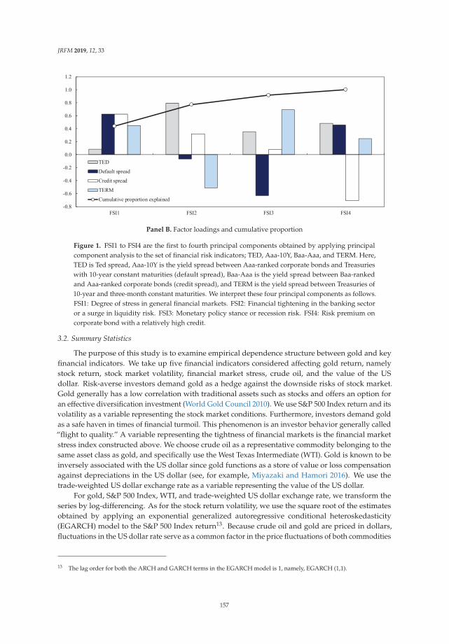
JRFM 2019, 12, 33
Panel B. Factor loadings and cumulative proportion
Figure 1. FSI1 to FSI4 are the first to fourth principal components obtained by applying principalcomponent analysis to the set of financial risk indicators; TED, Aaa-10Y, Baa-Aaa, and TERM. Here,TED is Ted spread, Aaa-10Y is the yield spread between Aaa-ranked corporate bonds and Treasurieswith 10-year constant maturities (default spread), Baa-Aaa is the yield spread between Baa-rankedand Aaa-ranked corporate bonds (credit spread), and TERM is the yield spread between Treasuries of10-year and three-month constant maturities. We interpret these four principal components as follows.FSI1: Degree of stress in general financial markets. FSI2: Financial tightening in the banking sectoror a surge in liquidity risk. FSI3: Monetary policy stance or recession risk. FSI4: Risk premium oncorporate bond with a relatively high credit.
3.2. Summary Statistics
The purpose of this study is to examine empirical dependence structure between gold and keyfinancial indicators. We take up five financial indicators considered affecting gold return, namelystock return, stock market volatility, financial market stress, crude oil, and the value of the USdollar. Risk-averse investors demand gold as a hedge against the downside risks of stock market.Gold generally has a low correlation with traditional assets such as stocks and offers an option foran effective diversification investment (World Gold Council 2010). We use S&P 500 Index return and itsvolatility as a variable representing the stock market conditions. Furthermore, investors demand goldas a safe haven in times of financial turmoil. This phenomenon is an investor behavior generally called“flight to quality.” A variable representing the tightness of financial markets is the financial marketstress index constructed above. We choose crude oil as a representative commodity belonging to thesame asset class as gold, and specifically use the West Texas Intermediate (WTI). Gold is known to beinversely associated with the US dollar since gold functions as a store of value or loss compensationagainst depreciations in the US dollar (see, for example, Miyazaki and Hamori 2016). We use thetrade-weighted US dollar exchange rate as a variable representing the value of the US dollar.
For gold, S&P 500 Index, WTI, and trade-weighted US dollar exchange rate, we transform theseries by log-differencing. As for the stock return volatility, we use the square root of the estimatesobtained by applying an exponential generalized autoregressive conditional heteroskedasticity(EGARCH) model to the S&P 500 Index return13. Because crude oil and gold are priced in dollars,fluctuations in the US dollar rate serve as a common factor in the price fluctuations of both commodities
13 The lag order for both the ARCH and GARCH terms in the EGARCH model is 1, namely, EGARCH (1,1).
157
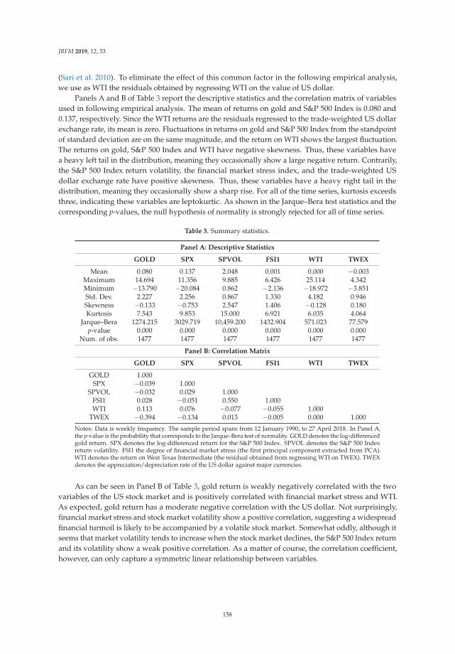
JRFM 2019, 12, 33
(Sari et al. 2010). To eliminate the effect of this common factor in the following empirical analysis,we use as WTI the residuals obtained by regressing WTI on the value of US dollar.
Panels A and B of Table 3 report the descriptive statistics and the correlation matrix of variablesused in following empirical analysis. The mean of returns on gold and S&P 500 Index is 0.080 and0.137, respectively. Since the WTI returns are the residuals regressed to the trade-weighted US dollarexchange rate, its mean is zero. Fluctuations in returns on gold and S&P 500 Index from the standpointof standard deviation are on the same magnitude, and the return on WTI shows the largest fluctuation.The returns on gold, S&P 500 Index and WTI have negative skewness. Thus, these variables havea heavy left tail in the distribution, meaning they occasionally show a large negative return. Contrarily,the S&P 500 Index return volatility, the financial market stress index, and the trade-weighted USdollar exchange rate have positive skewness. Thus, these variables have a heavy right tail in thedistribution, meaning they occasionally show a sharp rise. For all of the time series, kurtosis exceedsthree, indicating these variables are leptokurtic. As shown in the Jarque–Bera test statistics and thecorresponding p-values, the null hypothesis of normality is strongly rejected for all of time series.
Table 3. Summary statistics.
Panel A: Descriptive Statistics
GOLD SPX SPVOL FSI1 WTI TWEX
Mean 0.080 0.137 2.048 0.001 0.000 −0.003Maximum 14.694 11.356 9.885 6.426 25.114 4.342Minimum −13.790 −20.084 0.862 −2.136 −18.972 −3.851Std. Dev. 2.227 2.256 0.867 1.330 4.182 0.946Skewness −0.133 −0.753 2.547 1.406 −0.128 0.180Kurtosis 7.543 9.853 15.000 6.921 6.035 4.064
Jarque–Bera 1274.215 3029.719 10,459.200 1432.904 571.023 77.579p-value 0.000 0.000 0.000 0.000 0.000 0.000
Num. of obs. 1477 1477 1477 1477 1477 1477
Panel B: Correlation Matrix
GOLD SPX SPVOL FSI1 WTI TWEX
GOLD 1.000SPX −0.039 1.000
SPVOL −0.032 0.029 1.000FSI1 0.028 −0.051 0.550 1.000WTI 0.113 0.076 −0.077 −0.055 1.000
TWEX −0.394 −0.134 0.013 −0.005 0.000 1.000
Notes: Data is weekly frequency. The sample period spans from 12 January 1990, to 27 April 2018. In Panel A,the p-value is the probability that corresponds to the Jarque–Bera test of normality. GOLD denotes the log-differencedgold return. SPX denotes the log-differenced return for the S&P 500 Index. SPVOL denotes the S&P 500 Indexreturn volatility. FSI1 the degree of financial market stress (the first principal component extracted from PCA).WTI denotes the return on West Texas Intermediate (the residual obtained from regressing WTI on TWEX). TWEXdenotes the appreciation/depreciation rate of the US dollar against major currencies.
As can be seen in Panel B of Table 3, gold return is weakly negatively correlated with the twovariables of the US stock market and is positively correlated with financial market stress and WTI.As expected, gold return has a moderate negative correlation with the US dollar. Not surprisingly,financial market stress and stock market volatility show a positive correlation, suggesting a widespreadfinancial turmoil is likely to be accompanied by a volatile stock market. Somewhat oddly, although itseems that market volatility tends to increase when the stock market declines, the S&P 500 Index returnand its volatility show a weak positive correlation. As a matter of course, the correlation coefficient,however, can only capture a symmetric linear relationship between variables.
158
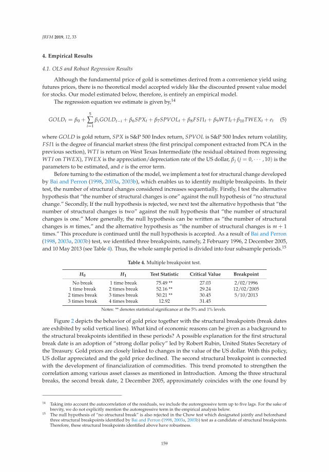
JRFM 2019, 12, 33
4. Empirical Results
4.1. OLS and Robust Regression Results
Although the fundamental price of gold is sometimes derived from a convenience yield usingfutures prices, there is no theoretical model accepted widely like the discounted present value modelfor stocks. Our model estimated below, therefore, is entirely an empirical model.
The regression equation we estimate is given by,14
GOLDt = β0 +5
∑i=1
βiGOLDt−i + β6SPXt + β7SPVOLt + β8FSI1t + β9WTIt+β10TWEXt + et (5)
where GOLD is gold return, SPX is S&P 500 Index return, SPVOL is S&P 500 Index return volatility,FSI1 is the degree of financial market stress (the first principal component extracted from PCA in theprevious section), WTI is return on West Texas Intermediate (the residual obtained from regressingWTI on TWEX), TWEX is the appreciation/depreciation rate of the US dollar, β j (j = 0, · · · , 10) is theparameters to be estimated, and e is the error term.
Before turning to the estimation of the model, we implement a test for structural change developedby Bai and Perron (1998, 2003a, 2003b), which enables us to identify multiple breakpoints. In theirtest, the number of structural changes considered increases sequentially. Firstly, I test the alternativehypothesis that “the number of structural changes is one” against the null hypothesis of “no structuralchange.” Secondly, If the null hypothesis is rejected, we next test the alternative hypothesis that “thenumber of structural changes is two” against the null hypothesis that “the number of structuralchanges is one.” More generally, the null hypothesis can be written as “the number of structuralchanges is m times,” and the alternative hypothesis as “the number of structural changes is m + 1times.” This procedure is continued until the null hypothesis is accepted. As a result of Bai and Perron(1998, 2003a, 2003b) test, we identified three breakpoints, namely, 2 February 1996, 2 December 2005,and 10 May 2013 (see Table 4). Thus, the whole sample period is divided into four subsample periods.15
Table 4. Multiple breakpoint test.
H0 H1 Test Statistic Critical Value Breakpoint
No break 1 time break 75.49 ** 27.03 2/02/19961 time break 2 times break 52.16 ** 29.24 12/02/20052 times break 3 times break 50.21 ** 30.45 5/10/20133 times break 4 times break 12.92 31.45
Notes: ** denotes statistical significance at the 5% and 1% levels.
Figure 2 depicts the behavior of gold price together with the structural breakpoints (break datesare exhibited by solid vertical lines). What kind of economic reasons can be given as a background tothe structural breakpoints identified in these periods? A possible explanation for the first structuralbreak date is an adoption of “strong dollar policy” led by Robert Rubin, United States Secretary ofthe Treasury. Gold prices are closely linked to changes in the value of the US dollar. With this policy,US dollar appreciated and the gold price declined. The second structural breakpoint is connectedwith the development of financialization of commodities. This trend promoted to strengthen thecorrelation among various asset classes as mentioned in Introduction. Among the three structuralbreaks, the second break date, 2 December 2005, approximately coincides with the one found by
14 Taking into account the autocorrelation of the residuals, we include the autoregressive term up to five lags. For the sake ofbrevity, we do not explicitly mention the autoregressive term in the empirical analysis below.
15 The null hypothesis of “no structural break” is also rejected in the Chow test which designated jointly and beforehandthree structural breakpoints identified by Bai and Perron (1998, 2003a, 2003b) test as a candidate of structural breakpoints.Therefore, these structural breakpoints identified above have robustness.
159
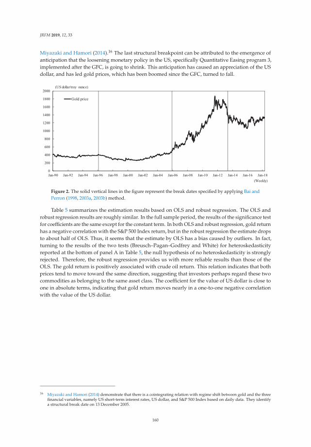
JRFM 2019, 12, 33
Miyazaki and Hamori (2014).16 The last structural breakpoint can be attributed to the emergence ofanticipation that the loosening monetary policy in the US, specifically Quantitative Easing program 3,implemented after the GFC, is going to shrink. This anticipation has caused an appreciation of the USdollar, and has led gold prices, which has been boomed since the GFC, turned to fall.
Figure 2. The solid vertical lines in the figure represent the break dates specified by applying Bai andPerron (1998, 2003a, 2003b) method.
Table 5 summarizes the estimation results based on OLS and robust regression. The OLS androbust regression results are roughly similar. In the full sample period, the results of the significance testfor coefficients are the same except for the constant term. In both OLS and robust regression, gold returnhas a negative correlation with the S&P 500 Index return, but in the robust regression the estimate dropsto about half of OLS. Thus, it seems that the estimate by OLS has a bias caused by outliers. In fact,turning to the results of the two tests (Breusch–Pagan–Godfrey and White) for heteroskedasticityreported at the bottom of panel A in Table 5, the null hypothesis of no heteroskedasticity is stronglyrejected. Therefore, the robust regression provides us with more reliable results than those of theOLS. The gold return is positively associated with crude oil return. This relation indicates that bothprices tend to move toward the same direction, suggesting that investors perhaps regard these twocommodities as belonging to the same asset class. The coefficient for the value of US dollar is close toone in absolute terms, indicating that gold return moves nearly in a one-to-one negative correlationwith the value of the US dollar.
16 Miyazaki and Hamori (2014) demonstrate that there is a cointegrating relation with regime shift between gold and the threefinancial variables, namely US short-term interest rates, US dollar, and S&P 500 Index based on daily data. They identifya structural break date on 13 December 2005.
160
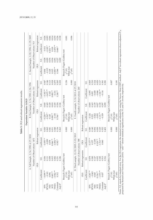
JRFM 2019, 12, 33
Ta
ble
5.
OLS
and
robu
stre
gres
sion
resu
lts.
Dep
en
den
tV
ari
ab
le:
GO
LD
A.F
ullS
ampl
e:2/
16/1
990–
4/27
/201
8B.
Firs
tSam
ple:
2/16
/199
0–1/
26/1
996
C.S
econ
dSa
mpl
e:2/
02/1
996–
11/2
5/20
05
Num
ber
ofO
bser
vati
ons:
1472
Num
ber
ofO
bser
vati
ons:
311
Num
ber
ofO
bser
vati
ons:
513
OLS
Rob
ustr
egre
ssio
nO
LSR
obus
treg
ress
ion
OLS
Rob
ustr
egre
ssio
n
Coe
ffici
ent
S.E.
Coe
ffici
ent
S.E.
Coe
ffici
ent
S.E.
Coe
ffici
ent
S.E.
Coe
ffici
ent
S.E.
Coe
ffici
ent
S.E.
SPX
−0.0
99**
0.03
6−0
.055
**0.
020
−0.2
28**
0.04
5−0
.182
**0.
047
0.00
40.
028
−0.0
110.
026
SPV
OL
−0.1
010.
111
−0.0
990.
063
−0.3
67*
0.16
5−0
.672
**0.
146
−0.1
150.
099
−0.1
83*
0.09
3FS
I10.
096
0.05
80.
078
0.04
10.
145
0.12
00.
160
0.11
30.
148
0.07
60.
201
**0.
066
WTI
0.06
5**
0.01
50.
046
**0.
011
0.09
0**
0.01
90.
083
**0.
018
0.01
50.
016
0.01
80.
014
TWEX
−0.9
62**
0.08
2−0
.892
**0.
048
−0.1
550.
105
−0.1
510.
079
−0.8
50**
0.09
1−0
.870
**0.
070
Con
stan
t0.
312
0.23
10.
302
*0.
136
0.74
4*
0.32
41.
240
**0.
265
0.34
40.
227
0.46
0*
0.22
6A
djR
20.
186
0.26
30.
126
0.23
20.
200
0.33
8
Breu
sch–
Paga
n–G
odfr
eyte
stBr
eusc
h–Pa
gan–
God
frey
test
Breu
sch–
Paga
n–G
odfr
eyte
stχ
2 (10)
0.00
0χ
2 (10)
0.13
6χ
2 (10)
0.00
1W
hite
test
Whi
tete
stW
hite
test
χ2 (
65)
0.00
0χ
2 (65)
0.00
0χ
2 (65)
0.00
6
D.T
hird
sam
ple:
12/0
2/20
05–5
/03/
2013
E.Fo
urth
sam
ple:
5/10
/201
3–4/
27/2
018
Num
ber
ofob
serv
atio
ns:3
88N
umbe
rof
obse
rvat
ions
:260
OLS
Rob
ustr
egre
ssio
nO
LSR
obus
treg
ress
ion
Coe
ffici
ent
S.E.
Coe
ffici
ent
S.E.
Coe
ffici
ent
S.E.
Coe
ffici
ent
S.E.
SPX
−0.2
67**
0.07
8−0
.177
**0.
049
−0.1
260.
069
−0.0
950.
065
SPV
OL
−0.0
630.
249
0.15
70.
149
0.22
20.
163
0.09
20.
210
FSI1
0.04
50.
127
−0.1
090.
092
−0.0
620.
139
−0.0
490.
164
WTI
0.15
4**
0.03
20.
129
**0.
030
−0.0
520.
027
−0.0
460.
029
TWEX
−1.5
73**
0.18
2−1
.513
**0.
129
−1.1
31**
0.13
0−1
.102
**0.
117
Con
stan
t0.
437
0.51
30.
060
0.32
2−0
.329
0.29
7−0
.116
0.36
1A
djR
20.
316
0.40
10.
299
0.38
1
Breu
sch–
Paga
n–G
odfr
eyte
stBr
eusc
h–Pa
gan–
God
frey
test
χ2 (
10)
0.00
0χ
2 (10)
0.00
7W
hite
test
Whi
tete
stχ
2 (65)
0.00
0χ
2 (65)
0.18
1
Not
es:S
.E.s
tand
sfo
rst
anda
rder
ror.
For
the
OLS
regr
essi
on,t
hest
anda
rder
rors
are
adju
sted
byus
ing
the
New
ey–W
est(
1987
)met
hod.
Adj
R2
for
robu
stre
gres
sion
show
sad
just
edR
2 Wpr
opos
edby
Ren
aud
and
Vic
tori
a-Fe
ser
(201
0).*
and
**de
note
stat
isti
cals
igni
fican
ceat
the
5%an
d1%
leve
ls,r
espe
ctiv
ely.
161

JRFM 2019, 12, 33
Then, we turn to the results of each subsample period. In the first sample, besides the returns onthe S&P 500 Index and WTI, the stock return volatility is estimated significantly. However, its sign isnegative and is opposite to the expected sign, whereas a significant relationship with the US dollar hasdisappeared. Breusch–Pagan–Godfrey and White tests present mixed evidence for heteroskedasticity,that is, the former cannot reject homoskedasticity hypothesis, while the latter reject the hypothesis.Therefore, we cannot clearly determine which of the OLS and robust regression results are reliable.In any case, however, estimated coefficients do not differ greatly in magnitude.
The second sample period has the largest number of observations among the four subsamples,and the OLS and robust regression results show some differences. In the OLS estimation, only the USdollar is significant, while in robust regression, stock return volatility is still negative and significant,and the rise in financial market stress works to push the gold return up significantly. The latter isconsistent with the expected sign. Both of two tests for heteroskedasticity reject the null hypothesis,suggesting that employing robust regression is adequate.
In the third and fourth subsamples, we find no noticeable difference when comparing bothestimation results. Although the results of the third sample period are similar to the those of thefull sample, the coefficients for the stock return, WTI, and US dollar are approximately two or threetimes larger than those in the full sample. This finding implies that the connection between goldand the financial variables has strengthened during this period, consistent with the financializationof commodities. Both of two tests for heteroskedasticity reject the null hypothesis, indicating thatresorting to robust regression is suitable.
For the fourth sample period, only the coefficient on the US dollar is negative and significant.Two tests for heteroskedasticity lead us to different conclusions, respectively, similar to the first sampleperiod. Although neither is significant, there are some differences in estimated coefficient of S&P 500Index volatility and constant term, between two methods.
In the following subsection, we present the results using quantile regression to explore therelationship in the tails of the distribution that cannot be captured by OLS and robust regressions.
4.2. Quantile Regression Results
4.2.1. Full Sample Period
Our quantile regression model corresponding to Equation (5) is given by,
GOLD(τ)t = β0(τ) +5∑
i=1βi(τ)GOLDt−i + β6(τ)SPXt + β7(τ)SPVOLt + β8(τ)FSI1t
+β9(τ)WTIt + β10(τ)TWEXt + et
(6)
where τ indicates the quantile level. Each coefficient takes a different estimate according to the quantilelevel. By looking at each of the subsample periods, we can examine the change in the conditional jointdistribution between gold return and each of financial indicators over time.
I present the estimation results for seven quantiles from 0.05 to 0.95 in Table 6. To compare theresults visually, Figure 3 graphically illustrates all the quantile processes.
162
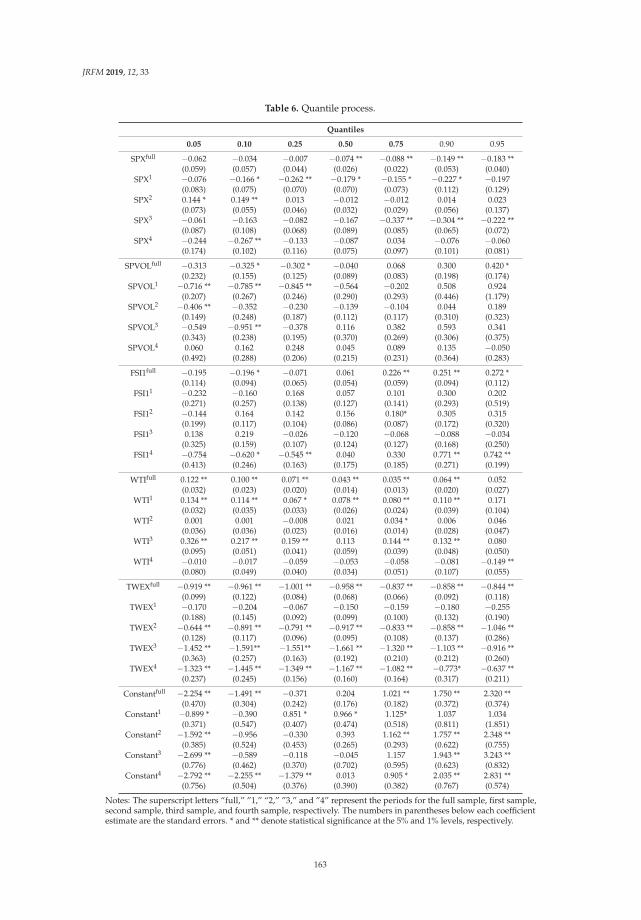
JRFM 2019, 12, 33
Table 6. Quantile process.
Quantiles
0.05 0.10 0.25 0.50 0.75 0.90 0.95
SPXfull −0.062 −0.034 −0.007 −0.074 ** −0.088 ** −0.149 ** −0.183 **(0.059) (0.057) (0.044) (0.026) (0.022) (0.053) (0.040)
SPX1 −0.076 −0.166 * −0.262 ** −0.179 * −0.155 * −0.227 * −0.197(0.083) (0.075) (0.070) (0.070) (0.073) (0.112) (0.129)
SPX2 0.144 * 0.149 ** 0.013 −0.012 −0.012 0.014 0.023(0.073) (0.055) (0.046) (0.032) (0.029) (0.056) (0.137)
SPX3 −0.061 −0.163 −0.082 −0.167 −0.337 ** −0.304 ** −0.222 **(0.087) (0.108) (0.068) (0.089) (0.085) (0.065) (0.072)
SPX4 −0.244 −0.267 ** −0.133 −0.087 0.034 −0.076 −0.060(0.174) (0.102) (0.116) (0.075) (0.097) (0.101) (0.081)
SPVOLfull −0.313 −0.325 * −0.302 * −0.040 0.068 0.300 0.420 *(0.232) (0.155) (0.125) (0.089) (0.083) (0.198) (0.174)
SPVOL1 −0.716 ** −0.785 ** −0.845 ** −0.564 −0.202 0.508 0.924(0.207) (0.267) (0.246) (0.290) (0.293) (0.446) (1.179)
SPVOL2 −0.406 ** −0.352 −0.230 −0.139 −0.104 0.044 0.189(0.149) (0.248) (0.187) (0.112) (0.117) (0.310) (0.323)
SPVOL3 −0.549 −0.951 ** −0.378 0.116 0.382 0.593 0.341(0.343) (0.238) (0.195) (0.370) (0.269) (0.306) (0.375)
SPVOL4 0.060 0.162 0.248 0.045 0.089 0.135 −0.050(0.492) (0.288) (0.206) (0.215) (0.231) (0.364) (0.283)
FSI1full −0.195 −0.196 * −0.071 0.061 0.226 ** 0.251 ** 0.272 *(0.114) (0.094) (0.065) (0.054) (0.059) (0.094) (0.112)
FSI11 −0.232 −0.160 0.168 0.057 0.101 0.300 0.202(0.271) (0.257) (0.138) (0.127) (0.141) (0.293) (0.519)
FSI12 −0.144 0.164 0.142 0.156 0.180* 0.305 0.315(0.199) (0.117) (0.104) (0.086) (0.087) (0.172) (0.320)
FSI13 0.138 0.219 −0.026 −0.120 −0.068 −0.088 −0.034(0.325) (0.159) (0.107) (0.124) (0.127) (0.168) (0.250)
FSI14 −0.754 −0.620 * −0.545 ** 0.040 0.330 0.771 ** 0.742 **(0.413) (0.246) (0.163) (0.175) (0.185) (0.271) (0.199)
WTIfull 0.122 ** 0.100 ** 0.071 ** 0.043 ** 0.035 ** 0.064 ** 0.052(0.032) (0.023) (0.020) (0.014) (0.013) (0.020) (0.027)
WTI1 0.134 ** 0.114 ** 0.067 * 0.078 ** 0.080 ** 0.110 ** 0.171(0.032) (0.035) (0.033) (0.026) (0.024) (0.039) (0.104)
WTI2 0.001 0.001 −0.008 0.021 0.034 * 0.006 0.046(0.036) (0.036) (0.023) (0.016) (0.014) (0.028) (0.047)
WTI3 0.326 ** 0.217 ** 0.159 ** 0.113 0.144 ** 0.132 ** 0.080(0.095) (0.051) (0.041) (0.059) (0.039) (0.048) (0.050)
WTI4 −0.010 −0.017 −0.059 −0.053 −0.058 −0.081 −0.149 **(0.080) (0.049) (0.040) (0.034) (0.051) (0.107) (0.055)
TWEXfull −0.919 ** −0.961 ** −1.001 ** −0.958 ** −0.837 ** −0.858 ** −0.844 **(0.099) (0.122) (0.084) (0.068) (0.066) (0.092) (0.118)
TWEX1 −0.170 −0.204 −0.067 −0.150 −0.159 −0.180 −0.255(0.188) (0.145) (0.092) (0.099) (0.100) (0.132) (0.190)
TWEX2 −0.644 ** −0.891 ** −0.791 ** −0.917 ** −0.833 ** −0.858 ** −1.046 **(0.128) (0.117) (0.096) (0.095) (0.108) (0.137) (0.286)
TWEX3 −1.452 ** −1.591** −1.551** −1.661 ** −1.320 ** −1.103 ** −0.916 **(0.363) (0.257) (0.163) (0.192) (0.210) (0.212) (0.260)
TWEX4 −1.323 ** −1.445 ** −1.349 ** −1.167 ** −1.082 ** −0.773* −0.637 **(0.237) (0.245) (0.156) (0.160) (0.164) (0.317) (0.211)
Constantfull −2.254 ** −1.491 ** −0.371 0.204 1.021 ** 1.750 ** 2.320 **(0.470) (0.304) (0.242) (0.176) (0.182) (0.372) (0.374)
Constant1 −0.899 * −0.390 0.851 * 0.966 * 1.125* 1.037 1.034(0.371) (0.547) (0.407) (0.474) (0.518) (0.811) (1.851)
Constant2 −1.592 ** −0.956 −0.330 0.393 1.162 ** 1.757 ** 2.348 **(0.385) (0.524) (0.453) (0.265) (0.293) (0.622) (0.755)
Constant3 −2.699 ** −0.589 −0.118 −0.045 1.157 1.943 ** 3.243 **(0.776) (0.462) (0.370) (0.702) (0.595) (0.623) (0.832)
Constant4 −2.792 ** −2.255 ** −1.379 ** 0.013 0.905 * 2.035 ** 2.831 **(0.756) (0.504) (0.376) (0.390) (0.382) (0.767) (0.574)
Notes: The superscript letters “full,” ”1,” “2,” ”3,” and ”4” represent the periods for the full sample, first sample,second sample, third sample, and fourth sample, respectively. The numbers in parentheses below each coefficientestimate are the standard errors. * and ** denote statistical significance at the 5% and 1% levels, respectively.
163
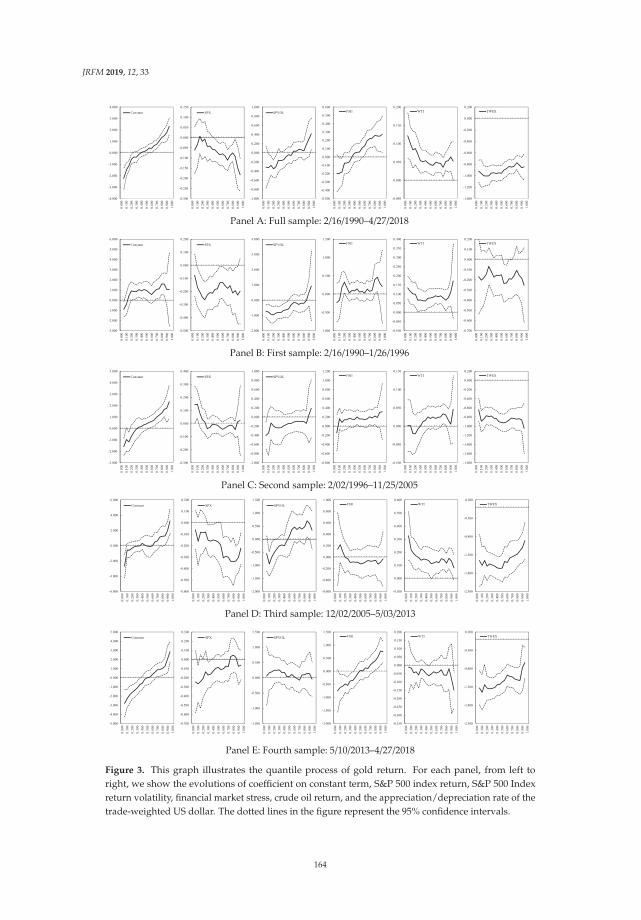
JRFM 2019, 12, 33
Panel A: Full sample: 2/16/1990–4/27/2018
Panel B: First sample: 2/16/1990–1/26/1996
Panel C: Second sample: 2/02/1996–11/25/2005
Panel D: Third sample: 12/02/2005–5/03/2013
Panel E: Fourth sample: 5/10/2013–4/27/2018
Figure 3. This graph illustrates the quantile process of gold return. For each panel, from left toright, we show the evolutions of coefficient on constant term, S&P 500 index return, S&P 500 Indexreturn volatility, financial market stress, crude oil return, and the appreciation/depreciation rate of thetrade-weighted US dollar. The dotted lines in the figure represent the 95% confidence intervals.
164

JRFM 2019, 12, 33
As shown in Panel A of Figure 3, Gold return is negatively correlated with the S&P 500 Indexreturn and is significantly negative from the intermediate quantiles to the upper quantiles. The higherthe quantile, the larger the coefficient increases in absolute value. The result means that gold returnwould rise largely when the stock return falls. However, the slope equality test at the lower and upperquantiles based on the Wald test cannot reject the null hypothesis of equality at 5% significance level,implying that dependence structures do not differ across quantile levels. Looking at the relationshipwith the stock return volatility, the estimated coefficient is negative for lower quantiles and positive forupper quantiles, implying that the gold return responds to the stock return volatility asymmetrically.The result that gold return rises as the stock market volatility increases is considered to reflect theinvestor behavior of divesting from stocks as a risky asset and demanding gold as a safety asset.Applying the Wald test, we can reject the slope equality hypothesis at 5% significance level, suggestingthat dependence structures are different across quantile levels. Analogous to stock return volatility,for the financial market stress, the estimated coefficient is negative for the lower quantiles and positivefor the upper quantiles, indicating asymmetric response of gold return to the degree of financial marketstress. The Wald test clearly rejects the null hypothesis of equality at 1% significance level again.In other words, when the general financial market tightens, gold returns rise, and this result reflectsthe flight-to-quality behavior of investors.
Regarding the relationships with crude oil and the value of the US dollar, no noticeable differenceis found from the results using OLS and robust regression. That is, the coefficient is significantlypositive from lower to upper quantiles for crude oil, whereas it is significantly negative from lowerto upper quantiles for the US dollar. The latter result is consistent with the findings of Miyazaki andHamori (2016).
In summary, quantile regression allows us to clarify the responses of gold return on stock returns,stock market volatility, and financial market tightness in the tails of the distribution. Such relationshipswere not captured by OLS and robust regressions. In the following, we present detailed results foreach subsample period.
4.2.2. Subsample Periods
For every explanatory variable, the confidence intervals are widened at the upper quantiles.Gold return shows a constantly negative correlation with the S&P 500 Index return and with crudeoil, regardless of quantile level. Gold return is negatively correlated with the stock return volatility atthe lower quantiles. There is no remarkable relationship between gold return and financial markettightness and between gold return and the value of US dollar.
As in the first sample period, the confidence intervals are widened at the upper quantiles forevery explanatory variable. We can observe a significant negative correlation between gold return andthe value of the US dollar from the lower to the upper quantile, but no notable relationship is foundfor other explanatory variables.
Our third sample period covers the outbreak of the GFC. As seen in Figure 3, the results for thisperiod are similar to those in the full sample period. The correlation between returns of gold and stockmarket is significantly negative from the intermediate quantiles to the upper quantiles. The negativecoefficient tends to become larger as the quantile increases. Unlike the full sample period, however,the Wald test during this sample period rejects the null hypothesis of equality at the 5% significancelevel, indicating that dependence structures differ across quantile values. Likewise, for the relationshipwith the stock market volatility, we can observe a similar pattern to those in the whole sample. That is,the coefficient is negative in lower quantiles positive in the upper quantiles. However, the resultof the Wald test shows that the null hypothesis of equality cannot be rejected marginally at the 5%significance level (p-value = 0.057). Thus, we obtain partial evidence that flight to quality of investors
165
JRFM 2019, 12, 33
from stock as a risky asset to gold as a safety asset had occurred.17 Similar arguments can be applied tocrude oil and the value of US dollar. In other words, gold return is constantly and positively correlatedwith crude oil irrespective of quantile level and is negatively associated with the US dollar throughoutthe quantiles. Surprisingly, gold return does not respond significantly to the degree of general financialmarket stress throughout the quantiles.
Finally, we confirm the results in the sample period after the GFC. At the lower quantiles,gold return is negatively associated with the stock return. Meanwhile, we find no noticeable relationbetween gold return and stock return volatility and between gold return and crude oil. For the USdollar, similar to other subsample periods except the first one, there is a significant negative correlationfrom the lower quantiles to upper quantiles. A noteworthy feature in this sample period is thatasymmetry is found in association with financial market risk; the coefficient is negative in the lowerquantiles and positive in the upper quantiles. This result tells us that as the general financial markettightens, gold return rises. The Wald test also strongly reinforces this result. That is, the null hypothesisof equality is rejected at the 1% significance level. Thus, we can say that the flight to quality and thedemand for gold as a safe haven by investors are phenomena that emerged recently. This finding isconsistent with Baur (2011), but the findings of this study refer to a much later phenomenon.18
5. Conclusions
In this study, we investigate how gold returns respond to changes in financial variables suchas stock returns and financial market conditions. In particular, in order to elaborate the behaviorin the tails of the distribution, we use quantile regression to confirm that gold return exhibits anasymmetric response depending on the quantile level. Specifically, according to our empirical results,gold return rises when; (1) stock return falls, (2) stock market volatility increases, and (3) the generalfinancial market tightens. Findings (1) and (2) are remarkable in the sample period covering the GFCand (3) is prominent in the sample after the GFC to the present. Furthermore, gold return showsalmost constant positive correlation with crude oil, and negative correlation with the value of theUS dollar. These results provide useful implications for portfolio selection of individual investors,risk management of financial institutions, and policymakers aiming for financial stability.
The analysis in this paper can be extended by explicitly incorporating the correlation with stockreturns into the model, as in Connolly et al. (2005). They analyze the relationships between returnson stocks and bonds under a regime-switching framework. Furthermore, performing out-of-sampleforecasting and evaluation of goodness of fit is also an important issue.19 Additionally, it is worthextending the model in this paper to predictive regression. Another way of extending of our analysisis to model the dependence structure by using copula or extreme value theory, which is now widelyapplied in the empirical finance literature. We leave these promising extensions for future research.
Funding: This research received no external funding.
Acknowledgments: I would like to thank two anonymous referees, whose insightful comments and suggestionshelped to improve an earlier draft of this paper.
Conflicts of Interest: The author declares no conflict of interest.
References
Agyei-Ampomah, Sam, Dimitrios Gounopoulos, and Khelifa Mazouz. 2014. Does gold offer a better protectionagainst losses in sovereign debt bonds than other metals? Journal of Banking & Finance 40: 507–21.
17 See also Miyazaki and Hamori (2013). They show that there exists a unilateral causality in not only the mean but the variancefrom stock return to gold return in the sample period post subprime crisis.
18 Although we do not dwell in the main text on the details of the results using FSI2, FSI3, and FSI4 as a financial stress index,all results are available from the author upon request.
19 I would like to thank an anonymous referee for raising this point.
166

JRFM 2019, 12, 33
Akram, Q. Farooq. 2009. Commodity prices, interest rates and the dollar. Energy Economics 31: 838–51. [CrossRef]Alkhatib, Akram, and Murad Harasheh. 2018. Performance of Exchange Traded Funds during the Brexit
referendum: An event study. International Journal of Financial Studies 6: 64. [CrossRef]Alexander, Carol. 2008. Market Risk Analysis: Practical Financial Econometrics (Vol. II). Hoboken: Wiley.Bai, Jushan, and Pierre Perron. 1998. Estimating and testing linear models with multiple structural changes.
Econometrica 66: 47–78. [CrossRef]Bai, Jushan, and Pierre Perron. 2003a. Computation and analysis of multiple structural change models. Journal of
Applied Econometrics 18: 1–22. [CrossRef]Bai, Jushan, and Pierre Perron. 2003b. Critical values for multiple structural change tests. The Econometrics Journal
6: 72–78. [CrossRef]Balcilar, Mehmet, Zeynel Abidin Ozdemir, and Huseyin Ozdemir. 2018. Dynamic Return and Volatility Spillovers
among S&P 500, Crude Oil and Gold. Discussion Paper 15–46. Famagusta: Eastern Mediterranean University,Department of Economics.
Basu, Parantap, and William T. Gavin. 2011. What explains the growth in commodity derivatives? Federal Bank ofSt. Louis Review 93: 37–48. [CrossRef]
Batten, Jonathan A., Cetin Ciner, and Brian M. Lucey. 2010. The macroeconomic determinants of volatility inprecious metals markets. Resources Policy 35: 65–71. [CrossRef]
Batten, Jonathan A., Cetin Ciner, and Brian M. Lucey. 2014. Which precious metals spill over on which, when andwhy? Some evidence. Applied Economics Letters 22: 466–73. [CrossRef]
Baur, Dirk G. 2011. Explanatory mining for gold: Contrasting evidence from simple and multiple regressions.Resources Policy 36: 265–75. [CrossRef]
Baur, Dirk G. 2013. The structure and degree of dependence: A quantile regression approach. Journal of Banking &Finance 37: 786–98.
Baur, Dirk G., and Niels Schulze. 2005. Coexceedances in financial markets—A quantile regression analysis ofcontagion. Emerging Markets Review 6: 21–43. [CrossRef]
Baur, Dirk G., and Brian M. Lucey. 2010. Is gold a hedge or a safe haven? An analysis of stocks, bonds and gold.Financial Review 45: 217–29. [CrossRef]
Baur, Dirk G., and Thomas K. McDermott. 2010. Is gold a safe haven? International evidence. Journal of Banking &Finance 34: 1886–98.
Bhar, Ramaprasad, and Shawkat Hammoudeh. 2011. Commodities and financial variables: Analyzingrelationships in a changing regime environment. International Review of Economics & Finance 20: 469–84.
Bouoiyour, Jamal, Refk Selmi, and Mark Wohar. 2018. Measuring the response of gold prices to uncertainty:An analysis beyond the mean. In Economic Modelling. Amsterdam: Elsevier, in press.
Chan, Kam Fong, Sirimon Treepongkaruna, Robert Brooks, and Stephen Gray. 2011. Asset market linkages:Evidence from financial, commodity and real estate assets. Journal of Banking & Finance 35: 1415–26.
Chao, Shih-Kang, Wolfgang K. Härdle, and Weining Wang. 2012. Quantile Regression in Risk Calibration. SFB 649Discussion Paper 2012-006. Berlin: Humboldt-Universität.
Cheng, Ing-Haw, and Wei Xiong. 2014. Financialization of commodity markets. Annual Review of FinancialEconomics 6: 419–41. [CrossRef]
Chevallier, Julien, and Florian Ielpo. 2013. Volatility spillovers in commodity markets. Applied Economics Letters 20:1211–27. [CrossRef]
Chudik, Alexander, and Marcel Fratzscher. 2011. Identifying the global transmission of the 2007–2009 financialcrisis in a GVAR model. European Economic Review 55: 325–39. [CrossRef]
Ciner, Cetin, Constantin Gurdgiev, and Brian M. Lucey. 2013. Hedges and safe havens: An examination of stocks,bonds, gold, oil, and exchange rates. International Review of Financial Analysis 29: 202–11. [CrossRef]
Cohen, Gil, and Mahmod Qadan. 2010. Is gold still a shelter to fear? American Journal of Social and ManagementSciences 1: 39–43. [CrossRef]
Connolly, Robert, Chris Stivers, and Licheng Sun. 2005. Stock market uncertainty and the stock-bond returnrelation. Journal of Financial and Quantitative Analysis 40: 161–94. [CrossRef]
Cont, Rama. 2001. Empirical properties of asset returns: Stylized facts and statistical issues. Quantitative Finance 1:223–36. [CrossRef]
Diebold, Francis X., and Kamil Yilmaz. 2012. Better to give than to receive: Predictive directional measurement ofvolatility spillovers. International Journal of Forecasting 28: 57–66. [CrossRef]
167

JRFM 2019, 12, 33
Domanski, Dietrich, and Alexandra Heath. 2007. Financial investors and commodity markets. BIS QuarterlyReview 3: 53–67.
Ehrmann, Michael, Marcel Fratzscher, and Roberto Rigobon. 2011. Stocks, bonds, money markets, and exchangerates: Measuring international financial transmission. Journal of Applied Econometrics 26: 948–74. [CrossRef]
Erb, Claude B., and Campbell R. Harvey. 2006. The strategic and tactical value of commodity futures. FinancialAnalysts Journal 62: 69–97. [CrossRef]
Fabozzi, Frank J., Sergio M. Focardi, Svetlozar T. Rachev, and Bala G. Arshanapalli. 2014. The Basics of FinancialEconometrics: Tools, Concepts, and Asset Management Applications. Hoboken: John Wiley & Sons, Inc.
Franke, Jürgen, Peter Mwita, and Weining Wang. 2015. Nonparametric estimates for conditional quantiles of timeseries. AStA Advances in Statistical Analysis 99: 107–30. [CrossRef]
Gorton, Gary, and K. Geert Rouwenhorst. 2006. Facts and fantasies about commodity futures. Financial AnalystsJournal 62: 47–68. [CrossRef]
Guo, Feng, Carl R. Chen, and Ying Sophie Huang. 2011. Markets contagion during financial crisis:A regime-switching approach. International Review of Economics & Finance 20: 95–109.
Hammoudeh, Shawkat, Ramazan Sari, and Bradley T. Ewing. 2009. Relationships among strategic commoditiesand with financial variables: A new look. Contemporary Economic Policy 27: 251–64. [CrossRef]
Hao, Lingxin, and Daniel Q. Naiman. 2007. Quantile Regression. Quantitative Applications in the Social Sciences,No. 149. Thousand Oaks: SAGE Publications, Inc.
Hartmann, Philipp, Stefan Straetmans, and C. G. de Vries. 2004. Asset market linkages in crisis periods. Review ofEconomics and Statistics 86: 313–26. [CrossRef]
Hillier, David, Paul Draper, and Robert Faff. 2006. Do precious metals shine? An investment perspective. FinancialAnalysts Journal 62: 98–106. [CrossRef]
Hood, Matthew, and Farooq Malik. 2013. Is gold the best hedge and a safe haven under changing stock marketvolatility? Review of Financial Economics 22: 47–52. [CrossRef]
IHS Global Inc. 2016. EViews 9 User’s Guide II. California: IHS Global Inc.Koenker, Roger, and Gilbert Bassett Jr. 1978. Regression quantiles. Econometrica 46: 33–50. [CrossRef]Koenker, Roger, and Kevin F. Hallock. 2001. Quantile regression. Journal of Economic Perspectives 15: 143–56.
[CrossRef]Longstaff, Francis A. 2010. The subprime credit crisis and contagion in financial markets. Journal of Financial
Economics 97: 436–50. [CrossRef]Mensi, Walid, Makram Beljid, Adel Boubaker, and Shunsuke Managi. 2013. Correlations and volatility spillovers
across commodity and stock markets: Linking energies, food, and gold. Economic Modelling 32: 15–22.[CrossRef]
Mensi, Walid, Shawkat Hammoudeh, Juan C. Reboredo, and Duc K. Nguyen. 2014. Do global factors impactBRICS stock markets? A quantile regression approach. Emerging Markets Review 19: 1–17. [CrossRef]
Miyazaki, Takashi, and Shigeyuki Hamori. 2013. Testing for causality between the gold return and stock marketperformance: Evidence for “gold investment in case of emergency”. Applied Financial Economics 23: 27–40.[CrossRef]
Miyazaki, Takashi, and Shigeyuki Hamori. 2014. Cointegration with regime shift between gold and financialvariables. International Journal of Financial Research 5: 90–97. [CrossRef]
Miyazaki, Takashi, and Shigeyuki Hamori. 2016. Asymmetric correlations in gold and other financial markets.Applied Economics 48: 4419–25. [CrossRef]
Miyazaki, Takashi, and Shigeyuki Hamori. 2018. The determinants of a simultaneous crash in gold and stockmarkets: An ordered logit approach. Annals of Financial Economics 13: 1850004. [CrossRef]
Miyazaki, Takashi, Yuki Toyoshima, and Shigeyuki Hamori. 2012. Exploring the dynamic interdependencebetween gold and other financial markets. Economics Bulletin 32: 37–50.
O’Connor, Fergal A., Brian M. Lucey, Jonathan A. Batten, and Dirk G. Baur. 2015. The financial economics ofgold—A survey. International Review of Financial Analysis 41: 186–205. [CrossRef]
Piplack, Jan, and Stefan Straetmans. 2010. Comovements of different asset classes during market stress. PacificEconomic Review 15: 385–400. [CrossRef]
Qadan, Mahmod, and Joseph Yagil. 2012. Fear sentiments and gold price: Testing causality in-mean andin-variance. Applied Economics Letters 19: 363–66. [CrossRef]
168

JRFM 2019, 12, 33
Raza, Syed Ali, Nida Shah, and Muhammad Shahbaz. 2018. Does economic policy uncertainty influencegold prices? Evidence from a nonparametric causality-in-quantiles approach. Resources Policy 57: 61–68.[CrossRef]
Reboredo, Juan C., and Gazi Salah Uddin. 2016. Do financial stress and policy uncertainty have an impact on theenergy and metals markets? A quantile regression approach. International Review of Economics & Finance 43:284–98.
Renaud, Olivier, and Maria-Pia Victoria-Feser. 2010. A robust coefficient of determination for regression. Journal ofStatistical Planning and Inference 140: 1852–62. [CrossRef]
Rodriguez, Robert N., and Yonggang Yao. 2017. Five Things You Should Know about Quantile Regression.Paper SAS525–2017. Cary: SAS Institute Inc.
Sari, Ramazan, Shawkat Hammoudeh, and Ugur Soytas. 2010. Dynamics of oil price, precious metal prices, andexchange rate. Energy Economics 32: 351–62. [CrossRef]
Silvennoinen, Annastiina, and Susan Thorp. 2013. Financialization, crisis, and commodity correlation dynamics.Journal of International Financial Markets, Institutions & Money 24: 42–65.
Straetmans, Stefan T. M., Willem F. C. Verschoor, and Christian C. P. Wolff. 2008. Extreme US stock marketfluctuations in the wake of 9/11. Journal of Applied Econometrics 23: 17–42. [CrossRef]
Tang, Ke, and Wei Xiong. 2012. Index investment and the financialization of commodities. Financial AnalystsJournal 68: 54–74. [CrossRef]
Wheelock, David C., and Mark E. Wohar. 2009. Can the term spread predict output growth and recessions?A survey of the literature. In Federal Reserve Bank of St. Louis Review 91. St. Louis: Federal Reserve Bank.
World Gold Council. 2010. Gold: Hedging against Tail Risk. London: World Gold Council.
© 2019 by the author. Licensee MDPI, Basel, Switzerland. This article is an open accessarticle distributed under the terms and conditions of the Creative Commons Attribution(CC BY) license (http://creativecommons.org/licenses/by/4.0/).
169
Journal of
Risk and FinancialManagement
Article
Testing for Causality-In-Mean and Variance betweenthe UK Housing and Stock Markets
Yuki Toyoshima
Shinsei Bank, Limited, 4-3, Nihonbashi-muromachi 2-chome, Chuo-ku, Tokyo 103-8303, Japan;[email protected]
Received: 24 March 2018; Accepted: 6 April 2018; Published: 26 April 2018
Abstract: This paper employs the two-step procedure to analyze the causality-in-mean andcausality-in-variance between the housing and stock markets of the UK. The empirical findingsmake two key contributions. First, although previous studies have indicated a one-way causalrelation from the housing market to the stock market in the UK, this paper discovered a two-waycausal relation between them. Second, a causality-in-variance as well as a causality-in-mean wasdetected from the housing market to the stock market.
Keywords: causality-in-variance; cross-correlation function; housing and stock markets
JEL Classification: C22; E44; G11
1. Introduction
Although major financial institutions experienced the subprime mortgage crisis and LehmanBrothers went out of business, the market for real estate has grown steadily in the last decade.As indicated in Figure 1, the UK is one of the largest markets in the world, followed by the US, Japan,Australia, and France. In addition, since the UK decided to withdraw from the European Union(“Brexit”), based on a referendum conducted on 23 June 2016, market participants and macroeconomicpolicymakers have focused more on its impact on the UK real estate market. Therefore, examining therelation between the UK real estate and other financial markets is useful for both practitioners andacademic researchers. Many previous empirical studies have explored the relation between the realestate and stock markets. Regarding this relation, we need to understand the following two effects.First, researchers who support the “wealth effect” claim that households benefiting from unanticipatedgains in stock prices tend to increase housing demand. Second, researchers who support the “creditprice effect” claim that an increase in real estate prices can stimulate economic activity and the futureprofitability of companies by raising the value of collateral and reducing the cost of borrowing for bothcompanies and households. Thus, identifying the direction of causality between the real estate andstock markets as well as the number of lags is essential.
As mentioned above, many previous empirical studies have analyzed the relation between the realestate and stock markets (e.g., Gyourko and Keim (1992); Ibbotson and Siegel (1984); Ibrahim (2010);Kapopoulos and Siokis (2005); Lin and Fuerst (2014); Liow (2006); Liow (2012); Liow and Yang (2005);Louis and Sun (2013); Okunev and Wilson (1997); Okunev et al. (2000); Quan and Titman (1999);Su (2011); and Tsai et al. (2012)). To the best of our knowledge, no studies have analyzed thecausality-in-variance between the real estate and stock markets. As indicated by Ross (1989), volatilityprovides useful data on the flow of information. For institutional investors such as banks, life insurancecompanies, hedge funds, and pension funds, deeper knowledge of spillover mechanisms for volatilitycan be useful for diversifying investments and hedge risk.
JRFM 2018, 11, 21; doi:10.3390/jrfm11020021 www.mdpi.com/journal/jrfm170
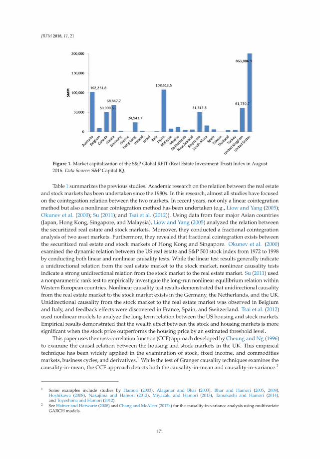
JRFM 2018, 11, 21
Figure 1. Market capitalization of the S&P Global REIT (Real Estate Investment Trust) Index in August2016. Data Source: S&P Capital IQ.
Table 1 summarizes the previous studies. Academic research on the relation between the real estateand stock markets has been undertaken since the 1980s. In this research, almost all studies have focusedon the cointegration relation between the two markets. In recent years, not only a linear cointegrationmethod but also a nonlinear cointegration method has been undertaken (e.g., Liow and Yang (2005);Okunev et al. (2000); Su (2011); and Tsai et al. (2012)). Using data from four major Asian countries(Japan, Hong Kong, Singapore, and Malaysia), Liow and Yang (2005) analyzed the relation betweenthe securitized real estate and stock markets. Moreover, they conducted a fractional cointegrationanalysis of two asset markets. Furthermore, they revealed that fractional cointegration exists betweenthe securitized real estate and stock markets of Hong Kong and Singapore. Okunev et al. (2000)examined the dynamic relation between the US real estate and S&P 500 stock index from 1972 to 1998by conducting both linear and nonlinear causality tests. While the linear test results generally indicatea unidirectional relation from the real estate market to the stock market, nonlinear causality testsindicate a strong unidirectional relation from the stock market to the real estate market. Su (2011) useda nonparametric rank test to empirically investigate the long-run nonlinear equilibrium relation withinWestern European countries. Nonlinear causality test results demonstrated that unidirectional causalityfrom the real estate market to the stock market exists in the Germany, the Netherlands, and the UK.Unidirectional causality from the stock market to the real estate market was observed in Belgiumand Italy, and feedback effects were discovered in France, Spain, and Switzerland. Tsai et al. (2012)used nonlinear models to analyze the long-term relation between the US housing and stock markets.Empirical results demonstrated that the wealth effect between the stock and housing markets is moresignificant when the stock price outperforms the housing price by an estimated threshold level.
This paper uses the cross-correlation function (CCF) approach developed by Cheung and Ng (1996)to examine the causal relation between the housing and stock markets in the UK. This empiricaltechnique has been widely applied in the examination of stock, fixed income, and commoditiesmarkets, business cycles, and derivatives.1 While the test of Granger causality techniques examines thecausality-in-mean, the CCF approach detects both the causality-in-mean and causality-in-variance.2
1 Some examples include studies by Hamori (2003), Alaganar and Bhar (2003), Bhar and Hamori (2005, 2008),Hoshikawa (2008), Nakajima and Hamori (2012), Miyazaki and Hamori (2013), Tamakoshi and Hamori (2014),and Toyoshima and Hamori (2012).
2 See Hafner and Herwartz (2008) and Chang and McAleer (2017a) for the causality-in-variance analysis using multivariateGARCH models.
171

JRFM 2018, 11, 21
The CCF approach can detect the direction of causality as well as the number of leads/lagsinvolved.3 Furthermore, it permits flexible specification of the innovation process and nondependenceon normality.4
Table 1. Summaries of previous studies.
Authors Empirical Technique Country Principal Results
Gyourko and Keim(1992) Market regression model the US Lagged equity REIT and stock return are predictors
of property index.
Ibbotson and Siegel(1984) Correlation, Regression the US Low correlation between the real estate and stocks,
bonds is found.
Ibrahim (2010) VAR model, Grangercausality tests Thailand Unidirectional causality from stock prices to house
prices is found.
Kapopoulos and Siokis(2005)
VAR model, Grangercausality tests Greece Unidirectional causality from stock prices to house
prices is found.
Lin and Fuerst (2014) Johansen, Gregory-Hansen,Nonlinear cointegration tests 9 Asian countries Market segmentation is observed in China, Japan,
Thailand, Malaysia, Indonesia and South Korea.
Liow (2006) ARDL cointegration tests SingaporeContemporaneous long-term relationship between
thestock market, residential and office propertyprices is found.
Liow (2012) Asymmetric DCC model 8 Asian countries Conditional real estate-stock correlations are timevarying and asymmetric in some cases.
Liow and Yang (2005) FIVEC model, VEC model 4 Asian countries FIVECM improves the forecasting performanceover conventional VECM models.
Louis and Sun (2013) Fama–MacBeth procedure the US Firms’ long-term abnormal stock returns arenegatively related to past growth in housing prices.
Okunev and Wilson(1997) Cointegration tests the US Weak and nonlinear relationship between the stock
and real estate markets is found.
Okunev et al. (2000) Linear and nonlinearcausality tests the US
Strong uni-directional relationship from the stockmarket to the real estate market is found in
nonlinear causality test.
Quan and Titman (1999) Cross-sectional regression 17 countries Positive relation between real estate values andstock returns is found.
Su (2011) TEC model, Non-parametricrank test
8 Western Europeancountries
Unidirectional causality from the real estatemarkets to the stock market is found in the
Germany, Netherlands and the UK.
Tsai et al. (2012) M-TAR cointegration model the US Threshold cointegration relationship between thehousing market and the stock market is found.
The remainder of this paper is organized as follows. The next section presents the CCF approach.In the following sections, we discuss the data, descriptive statistics, and results of the unit root testsand provide a description of the autoregressive-exponential generalized autoregressive conditionalheteroskedasticity (AR-EGARCH) specification. Thereafter, we present the empirical results anddiscuss the findings. Finally, a summary and conclusion are presented in the closing section.
2. Empirical Techniques
Following Cheung and Ng (1996), suppose there are two stationary and ergodic time series, Xt andYt. When I1,t, I2,t, and It are three information sets defined by I1,t = (Xt, Xt−1, . . .), I2,t = (Yt, Yt−1, . . .),and It = (Xt, Xt−1, . . . , Yt, Yt−1, . . .), Y is said to cause X in the mean if
E[Xt|I1,t−1] �= E[Xt|It−1]. (1)
3 One purpose of this paper is to detect the number of leads/lags, so we do not adopt Hong (2001) approach.4 See also Hamori (2003).
172

JRFM 2018, 11, 21
Similarly, X is said to cause Y in the mean if
E[Yt|I2,t−1] �= E[Yt|It−1]. (2)
Feedback effect in the mean occurs if Y causes X in the mean and X causes Y in the mean. On theother hand, Y is said to cause X in the variance if
E[(Xt − μX,t)
2|I1,t−1
]�= E
[(Xt − μX,t)
2|It−1
], (3)
where μX,t denotes the mean of Xt conditioned on I1,t−1. Similarly, X is said to cause Y in the variance if
E[(Yt − μY,t)
2|I2,t−1
]�= E
[(Yt − μY,t)
2|It−1
], (4)
where μY,t denotes the mean of Yt conditioned on I2,t−1. Feedback effect in the variance occurs if Xcauses Y in the variance and Y causes X in the variance.
We impose the following structure in Equation (1) through Equation (4) to detect causality-in-meanand causality-in-variance. Suppose Xt and Yt are written as
Xt = μX,t +√
hX,tεt, (5)
Yt = μY,t +√
hY,tζt, (6)
where {εt} and {ζt} are two independent white noise processes with zero mean and unit variance.For the causality-in-mean test, we have the standardized innovation as follows:
ut = (Xt − μX,t)2/hX,t = ε2
t , (7)
νt = (Yt − μY,t)2/hY,t = ζ2
t , (8)
with εt and ζt being the standardized residuals. Since these residuals are unobservable, we usetheir estimates. Next, using their estimates, we calculate the sample cross-correlation of thesquared standardized residual series, ruν(k), and the sample cross-correlation caluculated usingthe standardized residual series, rεζ(k), at time lag k.
The quantities rεζ(k) and ruν(k) are used to detect causality-in-mean and causality-in-variance,respectively, using the CCF approach.
First, we can detect the null hypothesis that there is no causality-in-mean using the followingCCF statistic:
CCF =√
T·rεζ(k). (9)
If the CCF test statistic is below the critical value calculated using the standard normal distribution,then we cannot reject the null hypothesis.
Second, we can detect the null hypothesis that there is no causality-in-variance using the teststatistic, which is given by
CCF =√
T·ruν(k). (10)
If the CCF test statistic is below the critical value calculated using the standard normal distribution,then we cannot reject the null hypothesis.
The CCF approach is divided into two steps. First, we estimate univariate time-series modelsthat consider the time variant conditional means and conditional variances. In this paper, we adoptthe AR-EGARCH formulation.5 Second, from the estimated AR-EGARCH model, we calculate the
5 See Nelson (1991).
173
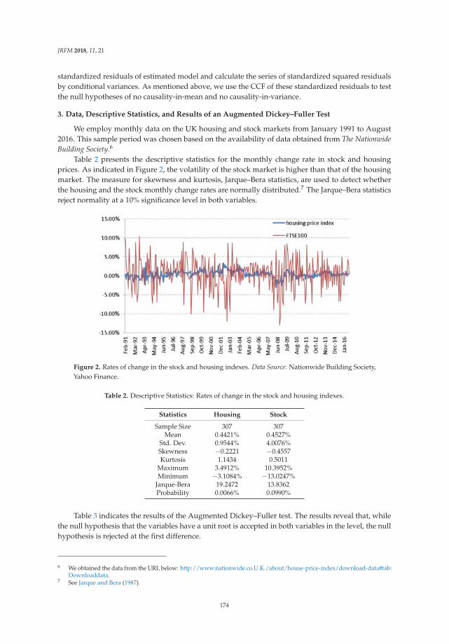
JRFM 2018, 11, 21
standardized residuals of estimated model and calculate the series of standardized squared residualsby conditional variances. As mentioned above, we use the CCF of these standardized residuals to testthe null hypotheses of no causality-in-mean and no causality-in-variance.
3. Data, Descriptive Statistics, and Results of an Augmented Dickey–Fuller Test
We employ monthly data on the UK housing and stock markets from January 1991 to August2016. This sample period was chosen based on the availability of data obtained from The NationwideBuilding Society.6
Table 2 presents the descriptive statistics for the monthly change rate in stock and housingprices. As indicated in Figure 2, the volatility of the stock market is higher than that of the housingmarket. The measure for skewness and kurtosis, Jarque–Bera statistics, are used to detect whetherthe housing and the stock monthly change rates are normally distributed.7 The Jarque–Bera statisticsreject normality at a 10% significance level in both variables.
Figure 2. Rates of change in the stock and housing indexes. Data Source: Nationwide Building Society,Yahoo Finance.
Table 2. Descriptive Statistics: Rates of change in the stock and housing indexes.
Statistics Housing Stock
Sample Size 307 307Mean 0.4421% 0.4527%
Std. Dev. 0.9544% 4.0076%Skewness −0.2221 −0.4557Kurtosis 1.1434 0.5011
Maximum 3.4912% 10.3952%Minimum −3.1084% −13.0247%
Jarque-Bera 19.2472 13.8362Probability 0.0066% 0.0990%
Table 3 indicates the results of the Augmented Dickey–Fuller test. The results reveal that, whilethe null hypothesis that the variables have a unit root is accepted in both variables in the level, the nullhypothesis is rejected at the first difference.
6 We obtained the data from the URL below: http://www.nationwide.co.U.K./about/house-price-index/download-data#tab:Downloaddata.
7 See Jarque and Bera (1987).
174

JRFM 2018, 11, 21
Table 3. Results of an augmented Dickey–Fuller test.
VariableAuxuliary Model
Const Const & Trend None
housing Level −0.2988 −2.3811 1.5701First difference −4.5065 *** −4.5019 *** −3.8047 ***
stockLevel −1.8598 −2.2418 0.7945
First difference −17.3975 *** −17.4146 *** −17.2370 ***
Notes: *** indicates significance at 1%.
4. Estimation of an AR-EGARCH Model
The first step of the CCF approach is to model the monthly change rates in the housing and stockprices. We estimate the AR(k)-EGARCH(p,q) model as follows:
yt = a0 + ∑ki=1 aiyt−i + b0Crisist + εt, εt/t−1 ∼ N(0, σ2
t ), (11)
Crisist =
{0 (t = Jan 91, . . . , May 07)1 (t = Jun 07, . . . , Aug16)
, (12)
log(σ2t ) = ω + ∑q
i=1(αi|Zt−i|+ γiZt−i) + ∑pi=1 βi log(σ2
t−i), (13)
where zt = εt/σt. Note that the left-hand side of Equation (13) is the log of the conditional variance.Using the log form of the EGARCH(p,q) model, it is possible to guarantee the non-negativity constraintswithout imposing the constraints of the coefficients.8 By including the term zt−i, the EGARCH(p,q)model reflects the asymmetric effect of positive and negative shocks. If γi > 0 then zt−1 = εt−1/σt−1 ispositive. The persistence of shocks to the conditional variance is given by ∑
pi=1 βi.
Equation (11), which is the conditional mean, is formulated as an autoregressive model of order k.To determine the optimal lag length k for each variables, we use the Schwartz–Bayesian InformationCriterion (SBIC).9. The SBIC is also applied in Equation (13) to determine the optimal lag lengthp and q.10
Table 4 presents the estimates for the AR(k)-EGARCH(p,q) model. Regarding the standarderror, this paper accepts the robust standard error developed by Bollerslev and Wooldridge (1992).First, the EGARCH(1,1) model is chosen for both variables. While all parameters of the EGARCHmodel in the monthly change rate in the stock price are significant, all parameters excluding γ1 in themonthly change rate in the housing price are significant at the conventional significance levels.
Furthermore, Table 4 reports the estimates of the coefficient β1, which measures the degree ofvolatility persistence. We find that β1 is significant at conventional significance levels, and the valueof β1 is close to 1. These estimates lead to the conclusion that the persistence in shocks to volatilityis relatively large. Table 2 also indicates the diagnostics of the empirical results of the AR-EGARCHmodel. While Q(24) is a test statistic for the null hypothesis that there is no autocorrelation up toorder 24 for standardized residuals, Q2(24) is a test statistic for the null hypothesis that there is noautocorrelation up to order 24 for standardized residuals squared.11 These tables show that bothstatistics are statistically significant at 5% level for all cases. Thus, the null hypothesis that there is noautocorrelation up to order 24 for standardized residuals and the standardized residuals squared isaccepted. These results empirically support the formulation of the AR-EGARCH model.
8 The EGARCH model suffers from a number of fundamental problems, including the lack of regularity conditions and hencethe absence of any asymptotic properties. See McAleer and Hafner (2014) and Chang and McAleer (2017b) for details.
9 See Schwarz (1978).10 We selected the final models from EGARCH(1,1), EGARCH(1,2), EGARCH(2,1), and EGARCH(2,2).11 See Ljung and Box (1978).
175
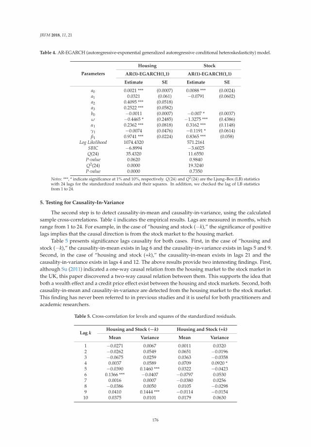
JRFM 2018, 11, 21
Table 4. AR-EGARCH (autoregressive-exponential generalized autoregressive conditional heteroskedasticity) model.
Parameters
Housing Stock
AR(3)-EGARCH(1,1) AR(1)-EGARCH(1,1)
Estimate SE Estimate SE
a0 0.0021 *** (0.0007) 0.0088 *** (0.0024)a1 0.0321 (0.061) −0.0791 (0.0602)a2 0.4095 *** (0.0518)a3 0.2522 *** (0.0582)b0 −0.0011 (0.0007) −0.007 * (0.0037)ω −0.4465 * (0.2485) −1.3275 *** (0.4386)α1 0.2362 *** (0.0818) 0.3162 *** (0.1148)γ1 −0.0074 (0.0476) −0.1191 * (0.0614)β1 0.9741 *** (0.0224) 0.8365 *** (0.058)
Log Likelihood 1074.4320 571.2161SBIC −6.8994 −3.6025Q(24) 35.4320 11.6550
P-value 0.0620 0.9840Q2(24) 0.0000 19.3240P-value 0.0000 0.7350
Notes: ***, * indicate significance at 1% and 10%, respectively. Q(24) and Q2(24) are the Ljung–Box (LB) statisticswith 24 lags for the standardized residuals and their squares. In addition, we checked the lag of LB statisticsfrom 1 to 24.
5. Testing for Causality-In-Variance
The second step is to detect causality-in-mean and causality-in-variance, using the calculatedsample cross-correlations. Table 4 indicates the empirical results. Lags are measured in months, whichrange from 1 to 24. For example, in the case of “housing and stock (−k),” the significance of positivelags implies that the causal direction is from the stock market to the housing market.
Table 5 presents significance lags causality for both cases. First, in the case of “housing andstock (−k),” the causality-in-mean exists in lag 6 and the causality-in-variance exists in lags 5 and 9.Second, in the case of “housing and stock (+k),” the causality-in-mean exists in lags 21 and thecausality-in-variance exists in lags 4 and 12. The above results provide two interesting findings. First,although Su (2011) indicated a one-way causal relation from the housing market to the stock market inthe UK, this paper discovered a two-way causal relation between them. This supports the idea thatboth a wealth effect and a credit price effect exist between the housing and stock markets. Second, bothcausality-in-mean and causality-in-variance are detected from the housing market to the stock market.This finding has never been referred to in previous studies and it is useful for both practitioners andacademic researchers.
Table 5. Cross-correlation for levels and squares of the standardized residuals.
Lag kHousing and Stock (−k) Housing and Stock (+k)
Mean Variance Mean Variance
1 −0.0271 0.0067 0.0011 0.03202 −0.0262 0.0549 0.0651 −0.01963 −0.0675 0.0259 0.0363 −0.03584 0.0037 0.0589 0.0709 0.0920 *5 −0.0390 0.1460 *** 0.0322 −0.04236 0.1366 *** −0.0407 −0.0797 0.05307 0.0016 0.0007 −0.0380 0.02568 −0.0386 0.0050 0.0105 −0.02989 0.0410 0.1444 *** −0.0114 −0.0154
10 0.0375 0.0101 0.0179 0.0630
176
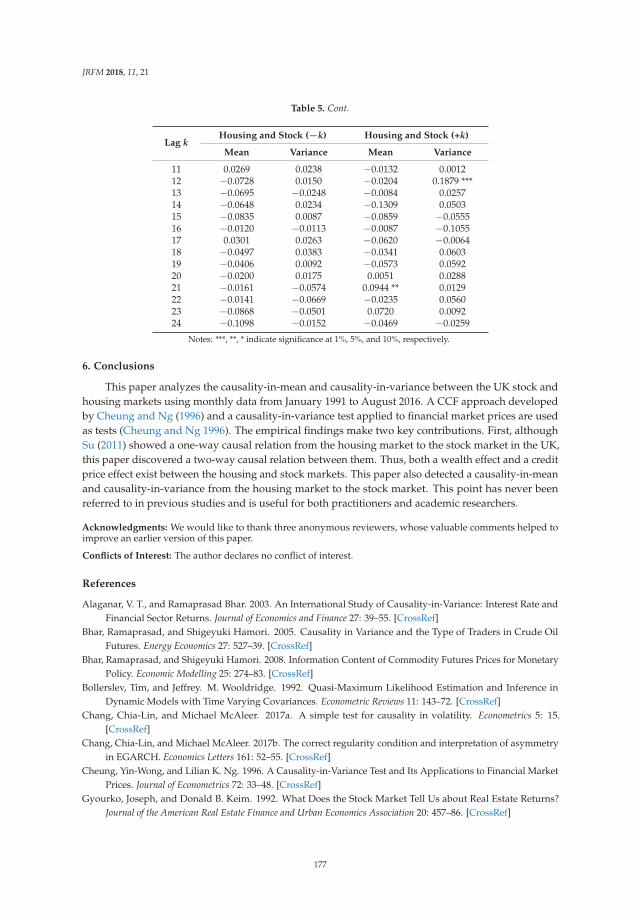
JRFM 2018, 11, 21
Table 5. Cont.
Lag kHousing and Stock (−k) Housing and Stock (+k)
Mean Variance Mean Variance
11 0.0269 0.0238 −0.0132 0.001212 −0.0728 0.0150 −0.0204 0.1879 ***13 −0.0695 −0.0248 −0.0084 0.025714 −0.0648 0.0234 −0.1309 0.050315 −0.0835 0.0087 −0.0859 −0.055516 −0.0120 −0.0113 −0.0087 −0.105517 0.0301 0.0263 −0.0620 −0.006418 −0.0497 0.0383 −0.0341 0.060319 −0.0406 0.0092 −0.0573 0.059220 −0.0200 0.0175 0.0051 0.028821 −0.0161 −0.0574 0.0944 ** 0.012922 −0.0141 −0.0669 −0.0235 0.056023 −0.0868 −0.0501 0.0720 0.009224 −0.1098 −0.0152 −0.0469 −0.0259
Notes: ***, **, * indicate significance at 1%, 5%, and 10%, respectively.
6. Conclusions
This paper analyzes the causality-in-mean and causality-in-variance between the UK stock andhousing markets using monthly data from January 1991 to August 2016. A CCF approach developedby Cheung and Ng (1996) and a causality-in-variance test applied to financial market prices are usedas tests (Cheung and Ng 1996). The empirical findings make two key contributions. First, althoughSu (2011) showed a one-way causal relation from the housing market to the stock market in the UK,this paper discovered a two-way causal relation between them. Thus, both a wealth effect and a creditprice effect exist between the housing and stock markets. This paper also detected a causality-in-meanand causality-in-variance from the housing market to the stock market. This point has never beenreferred to in previous studies and is useful for both practitioners and academic researchers.
Acknowledgments: We would like to thank three anonymous reviewers, whose valuable comments helped toimprove an earlier version of this paper.
Conflicts of Interest: The author declares no conflict of interest.
References
Alaganar, V. T., and Ramaprasad Bhar. 2003. An International Study of Causality-in-Variance: Interest Rate andFinancial Sector Returns. Journal of Economics and Finance 27: 39–55. [CrossRef]
Bhar, Ramaprasad, and Shigeyuki Hamori. 2005. Causality in Variance and the Type of Traders in Crude OilFutures. Energy Economics 27: 527–39. [CrossRef]
Bhar, Ramaprasad, and Shigeyuki Hamori. 2008. Information Content of Commodity Futures Prices for MonetaryPolicy. Economic Modelling 25: 274–83. [CrossRef]
Bollerslev, Tim, and Jeffrey. M. Wooldridge. 1992. Quasi-Maximum Likelihood Estimation and Inference inDynamic Models with Time Varying Covariances. Econometric Reviews 11: 143–72. [CrossRef]
Chang, Chia-Lin, and Michael McAleer. 2017a. A simple test for causality in volatility. Econometrics 5: 15.[CrossRef]
Chang, Chia-Lin, and Michael McAleer. 2017b. The correct regularity condition and interpretation of asymmetryin EGARCH. Economics Letters 161: 52–55. [CrossRef]
Cheung, Yin-Wong, and Lilian K. Ng. 1996. A Causality-in-Variance Test and Its Applications to Financial MarketPrices. Journal of Econometrics 72: 33–48. [CrossRef]
Gyourko, Joseph, and Donald B. Keim. 1992. What Does the Stock Market Tell Us about Real Estate Returns?Journal of the American Real Estate Finance and Urban Economics Association 20: 457–86. [CrossRef]
177

JRFM 2018, 11, 21
Hafner, Christian M., and Helmut Herwartz. 2008. Testing for Causality in Variance Using Multivariate GARCHModels. Annals of Economics and Statistics 89: 215–41. [CrossRef]
Hamori, Shigeyuki. 2003. An Empirical Investigation of Stock Markets: The CCF Approach. Dordrecht: KluwerAcademic Publishers.
Hong, Yongmiao. 2001. A Test for Volatility Spillover with Application to Exchange Rates. Journal of Econometrics103: 183–224. [CrossRef]
Hoshikawa, Takeshi. 2008. The Causal Relationships between Foreign Exchange Intervention and Exchange Rate.Applied Economics Letters 15: 519–22. [CrossRef]
Ibbotson, Roger G., and Laurence B. Siegel. 1984. Real Estate Returns: A Comparison with Other Investments.Real Estate Economics 12: 219–42. [CrossRef]
Ibrahim, Mansor H. 2010. House Price-Stock Price Relations in Thailand: An Empirical Analysis. InternationalJournal of Housing Markets and Analysis 3: 69–82. [CrossRef]
Jarque, Carlos M., and Anil K. Bera. 1987. Test for Normality of Observations and Regression Residuals.International Statistical Review 55: 163–72. [CrossRef]
Kapopoulos, Panayotis, and Fotios Siokis. 2005. Stock and Real Estate Prices in Greece: Wealth versus Credit-PriceEffect. Applied Economics Letters 12: 125–28. [CrossRef]
Lin, Pin-te, and Franz Fuerst. 2014. The Integration of Direct Real Estate and Stock Markets in Asia. AppliedEconomics 46: 1323–34. [CrossRef]
Liow, Kim Hiang, and Haishan Yang. 2005. Long-Term Co-Memories and Short-Run Adjustment: SecuritizedReal Estate and Stock Markets. The Journal of Real Estate Finance and Economics 31: 283–300. [CrossRef]
Liow, Kim Hiang. 2006. Dynamic Relationship between Stock and Property Markets. Applied Financial Economics16: 371–76. [CrossRef]
Liow, Kim Hiang. 2012. Co-Movements and Correlations Across Asian Securitized Real Estate and Stock Markets.Real Estate Economics 40: 97–129. [CrossRef]
Ljung, Greta M., and George E. P. Box. 1978. On a Measure of Lack of Fit in Time Series Models. Biometrika 66:265–70. [CrossRef]
Louis, Henock, and Amy X. Sun. 2013. Long-Term Growth in Housing Prices and Stock Returns. Real EstateEconomics 41: 663–708. [CrossRef]
McAleer, Michael, and Christian M. Hafner. 2014. A one line derivation of EGARCH. Econometrics 2: 92–97.[CrossRef]
Miyazaki, Takashi, and Shigeyuki Hamori. 2013. Testing for causality between the gold return and stock marketperformance: Evidence for gold investment in case of emergency. Applied Financial Economics 23: 27–40.[CrossRef]
Nakajima, Tadahiro, and Shigeyuki Hamori. 2012. Causality-in-Mean and Causality-in-Variance among ElectricityPrices, Crude Oil Prices, and Yen-US Dollar Exchange Rates in Japan. Research in International Business andFinance 26: 371–86. [CrossRef]
Nelson, Daniel B. 1991. Conditional Heteroskedasticity in Asset Returns: A New Approach. Econometrica 59:347–70. [CrossRef]
Okunev, John, and Patrick J. Wilson. 1997. Using Nonlinear Tests to Examine Integration between Real Estate andStock Markets. Real Estate Economics 25: 487–503. [CrossRef]
Okunev, John, Patrick Wilson, and Ralf Zurbruegg. 2000. The Causal Relationship between Real Estate and StockMarkets. Journal of Real Estate Finance and Economics 21: 251–61. [CrossRef]
Quan, Daniel C., and Sheridan Titman. 1999. Do Real Estate Prices and Stock Prices Move Together?An International Analysis. Real Estate Economics 27: 183–207. [CrossRef]
Ross, Stephen A. 1989. Information and Volatility: No-Arbitrage Martingale Approach to Timing and ResolutionIrrelevancy. Journal of Finance 44: 1–17. [CrossRef]
Su, Chi-Wei. 2011. Non-Linear Causality between the Stock and Real Estate Markets of Western EuropeanCountries: Evidence from Rank Tests. Economic Modelling 28: 845–51. [CrossRef]
Schwarz, Gideon. 1978. Estimating the Dimension of a Model. Annals of Statistics 6: 461–64. [CrossRef]Tsai, I-Chun, Cheng-Feng Lee, and Ming-Chu Chiang. 2012. The Asymmetric Wealth Effect in the U.S. Housing
and Stock Markets: Evidence from the Threshold Cointegration Model. Journal of Real Estate Finance andEconomics 45: 1005–20. [CrossRef]
178

JRFM 2018, 11, 21
Tamakoshi, Go, and Shigeyuki Hamori. 2014. Causality-in-variance and causality-in-mean between the Greeksovereignbond yields and Southern European banking sector equity returns. Journal of Economics and Finance38: 627–42. [CrossRef]
Toyoshima, Yuki, and Shigeyuki Hamori. 2012. Volatility Transmission of Swap Spreads among the United States,Japan, and the United Kingdom: A Cross-Correlation Function Approach. Applied Financial Economics 22:849–62. [CrossRef]
© 2018 by the author. Licensee MDPI, Basel, Switzerland. This article is an open accessarticle distributed under the terms and conditions of the Creative Commons Attribution(CC BY) license (http://creativecommons.org/licenses/by/4.0/).
179

Journal of
Risk and FinancialManagement
Article
Modeling the Dependence Structure of Share Pricesamong Three Chinese City Banks
Guizhou Liu, Xiao-Jing Cai and Shigeyuki Hamori *
Graduate School of Economics, Kobe University, 2-1, Rokkodai, Nada-Ku, Kobe 657-8501, Japan;[email protected] (G.L.); [email protected] (X.-J.C.)* Correspondence: [email protected]
Received: 23 August 2018; Accepted: 28 September 2018; Published: 29 September 2018
Abstract: We study the dependence structure of share price returns among the Beijing Bank, NingboBank, and Nanjing Bank using copula models. We use the normal, Student’s t, rotated Gumbel,and symmetrized Joe-Clayton (SJC) copula models to estimate the underlying dependence structure intwo periods: one covering the global financial crisis and the other covering the domestic share marketcrash in China. We show that Beijing Bank is less dependent on the other two city banks than NanjingBank, which is dependent on the other two in share price extreme returns. We also observe a majordecrease of dependency from 2007 to 2018 in three one-to-one dependence structures. Interestingly,contrary to recent literatures, Ningbo Bank and Nanjing Bank tend to be more dependent on eachother in positive returns than in negative returns during the past decade. We also show the dynamicdependence structures among three city banks using time-varying copula.
Keywords: city banks; dependence structure; copula
1. Introduction
Research on the co-movement among financial asset returns has tended to focus more on taildependence rather than linear correlation, as the former can capture the dependence structure ina period with extreme events (boom or crash). The dependence structure has been studied usingmany financial time series data, such as international share market indices, exchange rates, and bondyields; other non-financial data, such as oil and gold prices, have also been proven to be highly relatedto the tail dependence of financial markets. Furthermore, research on tail dependence has shownthat for most financial asset returns, there is more dependence during a crash than during boomperiods (see, for example, (Ang and Chen 2002)). Potential asymmetric characteristics exist in thetail dependence structure. For instance, as shown first by Patton (2006), some exchange rate returnsexhibit asymmetric tail dependence. These results relating to tail dependence aroused our interest inthe asymmetry in tail dependence.
In financial asset returns, tail dependence may change over time. As shown by Patton (2006),the tail dependence of DM (Deutsche mark)–USD (US dollar) and YEN (Japanese yen)–USD potentiallychanges over time, especially before and after the introduction of the Euro. Similarly, the exchange ratereturns reflect not only the financial market, but the consideration and behavior of the three centralbanks (such as motivating exports), especially before and after the introduction of the Euro. In thisstudy, we considered time-varying copula models to further capture the change of tail dependenceover time.
Little attention has been paid to the dependence structure among the share prices of city banks inChina. Share price returns are based on the prediction of not only macroeconomic variables, but alsoprofitability and risks, which are highly dependent on banking industry policies, bank strategies, localinvestment opportunities and risks, inter-bank lending, and inter-bank bond markets. The risks can be
JRFM 2018, 11, 57; doi:10.3390/jrfm11040057 www.mdpi.com/journal/jrfm180

JRFM 2018, 11, 57
passed from one bank to another, as indicated by tail dependence. The other banks, which includethe big four state-owned commercial banks, have large branches all over the country; these bankstend to have a more stable dependence structure and similar share price movements than city banks.Each city bank only has branches in the major cities and its own city where business first started.The dependence structure of city banks changes more obviously than that of the major banks. BeijingBank, Ningbo Bank, and Nanjing Bank were the earliest listed city banks in the Chinese share marketand have the largest data sample.
To investigate the underlying changes in dependence structure among the three city banks,we considered separating the sample and comparing the dependence strength in two distinct periods,as well as introducing time-varying copula models. The first step was to decide the proper separationof timing. In the past decade, the Chinese share market (Main Board) has experienced two largedeclines, one in the 2008 global financial crisis, and the other in the second half of 2015. The sharesof the three banks saw a large decline of more than 75% after being listed in the summer of 2007.All share prices reached close to the initial public offering (IPO) prices in the subsequent eight years.However, the prices shrank again to half in only two months during the domestic stock market crash.We separated the total sample at the start of the domestic stock market crash in June 2015.
This study makes two contributions. First, unlike most previous studies, we used copula modelson the city banks’ share price returns. Many scholars have used copula functions to capture thedependence structure and extend the models to asymmetric and time-varying ones, mostly onaggregate variables. Dependence structures have been widely discussed in terms of exchange rates(Patton 2006), carbon dioxide commission prices in international energy markets (Marimoutou andSoury 2015), oil prices and stock market indices (Sukcharoen et al. 2014), precious metal prices(Reboredo and Ugolini 2015), and international stock markets (Luo et al. 2011). Most of the studiesusing copula models were based on aggregate variables. Our study sheds new light on the dependencestructures among minor city banks based on various types of copula models. The second contributionis that we examined the changes in dependence structure of the daily share price returns betweenthe Beijing Bank, Ningbo Bank, and Nanjing Bank. Furthermore, the total sample was separatedinto two parts: (1) From 19 September 2007 to 4 June 2015, which covered the global financial crisis,and (2) from 12 June 2015 to 21 May 2018, which covered the domestic share market crash. Constantcopula models were used on the total sample and two distinct periods to compare the change inoverall correlation and tail dependence. Moreover, time-varying copula models were used to verifythe changes in dependence structure, mainly in tail dependence.
We present our conclusions in four parts. First, the share price returns of the Ningbo Bank andNanjing Bank had a higher dependency than the group of Ningbo Bank and Beijing Bank and thegroup of Nanjing Bank and Ningbo Bank. Second, a major decrease of dependence was found amongthe three city banks. However, the dependency of Ningbo Bank on Nanjing Bank seemed to be moreconsistent from 2008 to 2015 than the other two groups. Third, and most importantly, the joint increaseof the share prices of Ningbo Bank and Nanjing Bank happened more frequently than the joint decrease,which will shed new light on the research about financial assets price co-movement. Fourth, to betterdemonstrate the potential changes over time, the coefficients and figures of innovation were given inthe rotated Gumbel and Student’s t copula model (both in generalized autoregressive score [GAS]).The outcome of using the time-varying model suggested similar results in the constant copula models.Tail dependence rose rapidly in the beginning of period 1 and dropped in period 2.
The structure of the remaining paper is as follows: In Section 2, we introduce the basicmethodology applied in this study, including the marginal distribution models, the fundamentalcopula theory, and several copula functions. In Section 3, we first introduce the data sample and thedescriptive statistics, followed by the empirical results in constant and time-varying copula models.We discuss the dependence structure between Beijing Bank, Ningbo Bank, and Nanjing Bank in thetotal sample and in two distinct periods. In Section 4, we summarize our conclusions.
181
JRFM 2018, 11, 57
2. Empirical Methodology
This section begins with a discussion about the specific models for estimating the marginaldistribution, including the flexible skewed t and empirical distribution function (EDF). We then discussthe copula theory and some constant and time-varying copula models.
2.1. Models for Marginal Distributions
To model the dependence structure among the three city banks, we first had to model theconditional marginal distributions. Before modeling the marginal distributions, we documented thelog-difference of the share prices of the three city banks as daily returns. We modeled the time seriesdata with possible time-dependent conditional mean and variance. Orders of the ARMA model andstandard GARCH (1,1) model developed by Bollerslev (1987) were selected according to the BayesianInformation Criterion (BIC). The mean and variance models can be written in the forms given below.We denoted a given variable of daily returns as Yt and the returns shocks as εt. The standardizedresidual, ηt had a constant conditional distribution, where the mean was zero and variance was one.μi represents the estimated mean part of series i.
Yt = cy + ∑pi=1 φi,yYt−i + ∑q
j=1 θj,yεt−j + εt, εt =√
htηt, ηt ∼ iid(0, 1) (1)
ht = ω + βht−1 + αε2t−1, ηi,t = (Yi,t − μi)/
√hi,t, i = 1, 2, 3 (2)
It is a well-known fact that most financial time series data have fat tails and do not follow normaldistribution (Fama 1965). To better capture the possible fat tails feature, a Student’s t distribution isrecommended (Bollerslev 1987). We assumed that the term ηt followed a Student’s t distribution ratherthan a normal distribution. After estimating the marginal mean and variance models, we needed tomodel the distribution of estimated standardized residuals. We denoted the distribution function asFi. Following Patton (2013), we considered parametric and non-parametric models in modeling thedistribution of the standardized residuals in each financial data series. In the non-parametric model,we estimated Fi in EDF:
Fi(η) ≡ 1T + 1 ∑T
t=1 1{ηi,t ≤ η}, i = 1, 2, 3 (3)
In the parametric model, we followed the simple and flexible skewed t distribution developedby Hansen (1994). There are two parameters in this model: the first one is the skewness parameter,λ ∈ (−1, 1), and the second is the degrees of freedom parameter, ν ∈ (2, ∞); the two parameters controlthe degree of asymmetry and the fat tail feature. This model has many features. The distribution is askewed normal distribution when ν −→ ∞ , a standardized Student’s t distribution when λ = 0, and aN(0, 1) when λ = 0, ν −→ ∞ . In empirical study, the condition ν −→ ∞ occurs when ν is larger thansome level. After estimating the parametric model using the simple and flexible skewed t distribution,we carried out the goodness of fit (GoF) test on this result.
2.2. Constant Copula Models
We first describe the copula theory before analyzing the dependence structure. A key conceptwas presented by Sklar (1959), who indicated that joint distribution (F) in n dimensions could bedecomposed into the corresponding n univariate marginal distributions (Fi) and copula function(C : [0, 1]n −→ [0, 1] ) with n dimensions. Based on this foundation, another copula interpretation,the probability integral transformation (i.e., Ui ≡ Fi(Xi)) indicated by Casella and Berger (1990),has become popular in copula theory. After the transformation, variable Ui has a uniform f(0, 1)distribution that is unrelated to the original distribution Fi when Fi is continuous. After a vector ofprobability integral transformation U ≡ [U1, U2, · · · , Un] is obtained, C becomes a joint distributionfunction with uniform f(0, 1) distribution. Various copula models have been used to capture thedependence structure between time series data. However, the normal copula model cannot capture the
182

JRFM 2018, 11, 57
tail dependence because the tail dependence is assumed to be zero. Other forms of copula such as theGumbel and Clayton functions, can obtain tail dependence coefficients. Although the Gumbel (Clayton)copula can only obtain a non-zero (zero) upper tail dependence coefficient and a zero (non-zero) lowertail dependence coefficient, it can be further developed to the rotated-Gumbel (rotated-Clayton) toobtain the reverse tail dependence coefficient. We started with the selection of (constant) copulafunctions based on the rank of log-likelihood values. Normal, rotated-Gumbel, Student’s t, and SJCcopula functions were selected, and all were used in a bivariate case. We assumed that u1 and u2 werein the uniform distribution [0, 1]. Each copula model is briefly introduced below:
The normal copula function can be written as Equation (4), where θ is a linear correlationparameter and φ is a univariate standard normal distribution:
C(u1, u2) =∫ φ−1(u1)
−∞
∫ φ−1(u2)
−∞
1
2π√
1 − θ2exp(− s2 − 2θst + t2
2(1 − θ2))dsdt (4)
The Student’s t copula function can be defined as Equation (5), with v representing the degrees offreedom and t−1
v (·) being the inverse of a standard Student’s t distribution:
C(u1, u2) =∫ t−1
v (u1)
−∞
∫ t−1v (u2)
−∞
1
2π√
1 − θ2(1 +
s2 − 2θst + t2
v(1 − θ2))− v+2
v
dsdt (5)
The Gumbel copula (Gumbel 1960), concentrates on the upper tail dependence with zero lowertail dependence. It can be written in Equation (6) with parameter γ. In fact, there is abundant evidenceindicating that financial asset returns tend to have joint negative extremes (dramatic falls) more oftenthan joint positive extremes (sharp increases) (Patton 2006). Therefore, the rotated Gumbel functionmight be more practical than the Gumbel copula, where parameter γ is often calculated by denoting anew series as u′
1 = 1 − u1 and u′2 = 1 − u2, and the lower tail dependence will be 2 − 21/γ.
C(u1, u2) = exp{−[(−lnu1)γ + (−lnu2)
γ]1/γ}, γ ∈ (1,+∞) (6)
We considered the modified Clayton copula developed by Joe (1997), rather than the Claytoncopula. We refer to the transformed copula as the Joe–Clayton copula (Patton 2006). The Joe–Claytoncopula can be written in Equation (7), with τU ∈ (0, 1) and τL ∈ (0, 1) representing the upper andlower tail dependence, respectively. The parameters are κ = 1/log2(2 − τU) and γ = −1/log2(τ
L).
CJC(u1, u2|τU , τL) = 1 − (1 − {[1 − (1 − u1)κ]−γ
+[1 − (1 − u2)
κ]−γ − 1}−1/γ)
1/κ
(7)
As indicated by Patton (2006), asymmetry may still exist when the upper and lower taildependence strengths are equal in the Joe–Clayton copula. Owing to this major problem, we followedthe modification proposed by Patton (2006), which is denoted as the SJC copula:
CSJC(u1, u2|τU , τL) = 0.5(CJC(u1, u2|τU , τL) + CJC(1 − u1, 1 − u2|τL, τU) + u1 + u2 − 1) (8)
2.3. Time-Varying Copula Models
For analyzing the time-varying dependence strength, we considered using the rotated Gumbeland Student’s t copula models with the generalized autoregressive score (GAS) model introducedby Creal et al. (2013). In this model, a parameter δt is denoted as the time-varying copula parameter.The score of the likelihood in the copula is written as I−1/2
t st. Specifically, in the rotated Gumbelcopula model, the parameter δt = h−1( ft) can be defined as δt = 1 + exp ( ft) because the parametershould be larger than one. In the Student’s t copula model, the parameter can be defined asδt = (1 − exp{− ft})/(1 + exp{− ft}) to obtain the dependence parameter between −1 and 1.
183

JRFM 2018, 11, 57
ft = h(δt) ↔ δt = h−1( ft) (9)
where, ft+1 = ω + β ft + αI−1/2t st
st ≡ ∂
∂δlogc(U1t, U2t; δt), It ≡ Et−1
[sts′t]= I(δt)
3. Data and Empirical Results
3.1. Summary Statistics and Marginal Distributions
Our data contained the share price returns (based on adjusted prices) of three city banks in China:Beijing Bank, Ningbo Bank, and Nanjing Bank. The share prices and returns of these three city banksare shown in Figures 1 and 2. We chose these banks not only because they are among the top five citybanks in China, but also because they have stronger market liquidity in the Main Board share market,compared to that of other city banks. The share price data collected from IPOs in 2007 providedabundant data samples that covered the global financial crisis in 2008, as well as the China sharemarket crash in late 2015. We observed large declines in share prices and high variances in returnsduring the global financial crisis in 2008 and the domestic stock market crash in 2015. To explore thedependence structure among these three banks, we formed three combinations: Beijing Bank andNingbo Bank were Group 1, Beijing Bank and Nanjing Bank were Group 2, and Ningbo Bank andNanjing Bank were Group 3.
We computed the return rates of interest using the log-difference method with the n.a. values andoutliers deleted. We reported all relevant analyses in the total sample, first period sample, and secondperiod sample. The total sample ranged from 19 September 2007 to 21 May 2018. The first periodfrom 19 September 2007 to 4 June 2015 covered the 2008 global financial crisis. The second periodfrom 15 June 2015 to 21 May 2018 covered the domestic stock market crash from 12 June 2015 to19 February 2016. Descriptive statistics and the marginal distribution coefficients are given in Tables 1and 2, respectively.
Figure 1. Daily share prices of the Beijing Bank, Ningbo Bank, and Nanjing Bank from 19 September2007 to 21 May 2018.
184
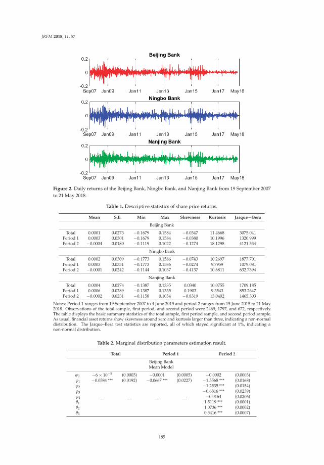
JRFM 2018, 11, 57
Figure 2. Daily returns of the Beijing Bank, Ningbo Bank, and Nanjing Bank from 19 September 2007to 21 May 2018.
Table 1. Descriptive statistics of share price returns.
Mean S.E. Min Max Skewness Kurtosis Jarque−Bera
Beijing Bank
Total 0.0001 0.0273 −0.1679 0.1584 −0.0347 11.4668 3075.041Period 1 0.0003 0.0301 −0.1679 0.1584 −0.0380 10.1996 1320.999Period 2 −0.0004 0.0180 −0.1119 0.1022 −0.1274 18.1298 4121.534
Ningbo Bank
Total 0.0002 0.0309 −0.1773 0.1586 −0.0743 10.2697 1877.701Period 1 0.0003 0.0331 −0.1773 0.1586 −0.0274 9.7959 1079.081Period 2 −0.0001 0.0242 −0.1144 0.1037 −0.4137 10.6811 632.7394
Nanjing Bank
Total 0.0004 0.0274 −0.1387 0.1335 0.0340 10.0755 1709.185Period 1 0.0006 0.0289 −0.1387 0.1335 0.1903 9.3543 853.2647Period 2 −0.0002 0.0231 −0.1158 0.1054 −0.8319 13.0402 1465.303
Notes: Period 1 ranges from 19 September 2007 to 4 June 2015 and period 2 ranges from 15 June 2015 to 21 May2018. Observations of the total sample, first period, and second period were 2469, 1797, and 672, respectively.The table displays the basic summary statistics of the total sample, first period sample, and second period sample.As usual, financial asset returns show skewness around zero and kurtosis larger than three, indicating a non-normaldistribution. The Jarque–Bera test statistics are reported, all of which stayed significant at 1%, indicating anon-normal distribution.
Table 2. Marginal distribution parameters estimation result.
Total Period 1 Period 2
Beijing BankMean Model
ϕ0 −6 × 10⁻⁵ (0.0003) −0.0001 (0.0005) −0.0002 (0.0003)ϕ1 −0.0584 *** (0.0192) −0.0667 *** (0.0227) −1.5568 *** (0.0168)ϕ2
— — — —
−1.2535 *** (0.0154)ϕ3 −0.6816 *** (0.0239)ϕ4 −0.0164 (0.0206)θ1 1.5119 *** (0.0001)θ2 1.0736 *** (0.0002)θ3 0.5416 *** (0.0007)
185
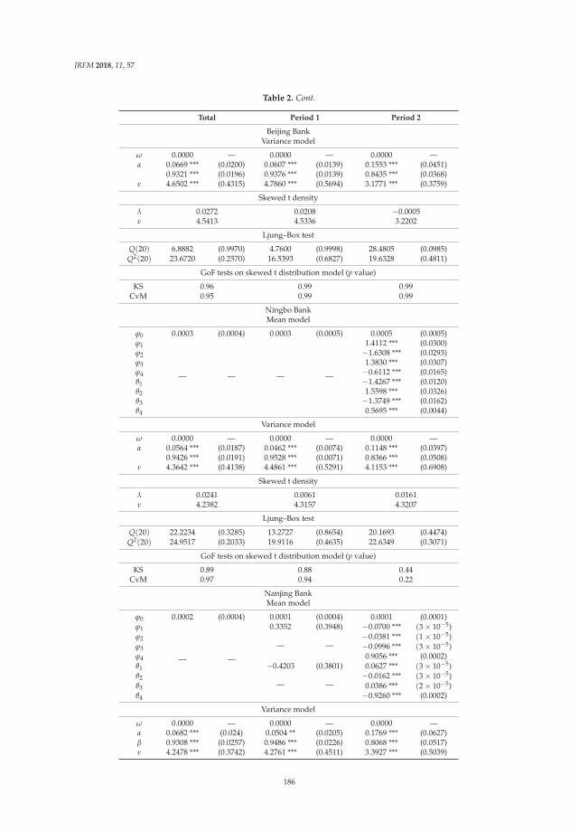
JRFM 2018, 11, 57
Table 2. Cont.
Total Period 1 Period 2
Beijing BankVariance model
ω 0.0000 — 0.0000 — 0.0000 —α 0.0669 *** (0.0200) 0.0607 *** (0.0139) 0.1553 *** (0.0451)
0.9321 *** (0.0196) 0.9376 *** (0.0139) 0.8435 *** (0.0368)ν 4.6502 *** (0.4315) 4.7860 *** (0.5694) 3.1771 *** (0.3759)
Skewed t density
λ 0.0272 0.0208 −0.0005ν 4.5413 4.5336 3.2202
Ljung–Box test
Q(20) 6.8882 (0.9970) 4.7600 (0.9998) 28.4805 (0.0985)Q2(20) 23.6720 (0.2570) 16.5393 (0.6827) 19.6328 (0.4811)
GoF tests on skewed t distribution model (p value)
KS 0.96 0.99 0.99CvM 0.95 0.99 0.99
Ningbo BankMean model
ϕ0 0.0003 (0.0004) 0.0003 (0.0005) 0.0005 (0.0005)ϕ1
— — — —
1.4112 *** (0.0300)ϕ2 −1.6308 *** (0.0293)ϕ3 1.3830 *** (0.0307)ϕ4 −0.6112 *** (0.0165)θ1 −1.4267 *** (0.0120)θ2 1.5598 *** (0.0326)θ3 −1.3749 *** (0.0162)θ4 0.5695 *** (0.0044)
Variance model
ω 0.0000 — 0.0000 — 0.0000 —α 0.0564 *** (0.0187) 0.0462 *** (0.0074) 0.1148 *** (0.0397)
0.9426 *** (0.0191) 0.9528 *** (0.0071) 0.8366 *** (0.0508)ν 4.3642 *** (0.4138) 4.4861 *** (0.5291) 4.1153 *** (0.6908)
Skewed t density
λ 0.0241 0.0061 0.0161ν 4.2382 4.3157 4.3207
Ljung–Box test
Q(20) 22.2234 (0.3285) 13.2727 (0.8654) 20.1693 (0.4474)Q2(20) 24.9517 (0.2033) 19.9116 (0.4635) 22.6349 (0.3071)
GoF tests on skewed t distribution model (p value)
KS 0.89 0.88 0.44CvM 0.97 0.94 0.22
Nanjing BankMean model
ϕ0 0.0002 (0.0004) 0.0001 (0.0004) 0.0001 (0.0001)ϕ1
— —
0.3352 (0.3948) −0.0700 *** (3 × 10⁻⁵)ϕ2
— —−0.0381 *** (1 × 10⁻⁵)
ϕ3 −0.0996 *** (3 × 10⁻⁵)ϕ4 0.9056 *** (0.0002)θ1 −0.4203 (0.3801) 0.0627 *** (3 × 10⁻⁵)θ2
— —−0.0162 *** (3 × 10⁻⁵)
θ3 0.0386 *** (2 × 10⁻⁵)θ4 −0.9260 *** (0.0002)
Variance model
ω 0.0000 — 0.0000 — 0.0000 —α 0.0682 *** (0.024) 0.0504 ** (0.0205) 0.1769 *** (0.0627)β 0.9308 *** (0.0257) 0.9486 *** (0.0226) 0.8068 *** (0.0517)ν 4.2478 *** (0.3742) 4.2761 *** (0.4511) 3.3927 *** (0.5039)
186
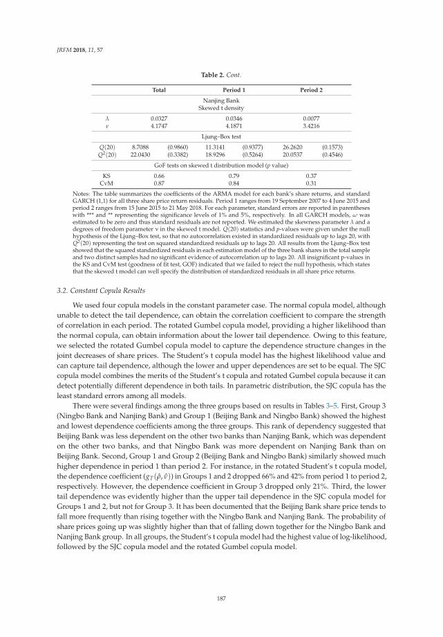
JRFM 2018, 11, 57
Table 2. Cont.
Total Period 1 Period 2
Nanjing BankSkewed t density
λ 0.0327 0.0346 0.0077ν 4.1747 4.1871 3.4216
Ljung–Box test
Q(20) 8.7088 (0.9860) 11.3141 (0.9377) 26.2620 (0.1573)Q2(20) 22.0430 (0.3382) 18.9296 (0.5264) 20.0537 (0.4546)
GoF tests on skewed t distribution model (p value)
KS 0.66 0.79 0.37CvM 0.87 0.84 0.31
Notes: The table summarizes the coefficients of the ARMA model for each bank’s share returns, and standardGARCH (1,1) for all three share price return residuals. Period 1 ranges from 19 September 2007 to 4 June 2015 andperiod 2 ranges from 15 June 2015 to 21 May 2018. For each parameter, standard errors are reported in parentheseswith *** and ** representing the significance levels of 1% and 5%, respectively. In all GARCH models, ω wasestimated to be zero and thus standard residuals are not reported. We estimated the skewness parameter λ and adegrees of freedom parameter ν in the skewed t model. Q(20) statistics and p-values were given under the nullhypothesis of the Ljung–Box test, so that no autocorrelation existed in standardized residuals up to lags 20, withQ2(20) representing the test on squared standardized residuals up to lags 20. All results from the Ljung–Box testshowed that the squared standardized residuals in each estimation model of the three bank shares in the total sampleand two distinct samples had no significant evidence of autocorrelation up to lags 20. All insignificant p-values inthe KS and CvM test (goodness of fit test, GOF) indicated that we failed to reject the null hypothesis, which statesthat the skewed t model can well specify the distribution of standardized residuals in all share price returns.
3.2. Constant Copula Results
We used four copula models in the constant parameter case. The normal copula model, althoughunable to detect the tail dependence, can obtain the correlation coefficient to compare the strengthof correlation in each period. The rotated Gumbel copula model, providing a higher likelihood thanthe normal copula, can obtain information about the lower tail dependence. Owing to this feature,we selected the rotated Gumbel copula model to capture the dependence structure changes in thejoint decreases of share prices. The Student’s t copula model has the highest likelihood value andcan capture tail dependence, although the lower and upper dependences are set to be equal. The SJCcopula model combines the merits of the Student’s t copula and rotated Gumbel copula because it candetect potentially different dependence in both tails. In parametric distribution, the SJC copula has theleast standard errors among all models.
There were several findings among the three groups based on results in Tables 3–5. First, Group 3(Ningbo Bank and Nanjing Bank) and Group 1 (Beijing Bank and Ningbo Bank) showed the highestand lowest dependence coefficients among the three groups. This rank of dependency suggested thatBeijing Bank was less dependent on the other two banks than Nanjing Bank, which was dependenton the other two banks, and that Ningbo Bank was more dependent on Nanjing Bank than onBeijing Bank. Second, Group 1 and Group 2 (Beijing Bank and Ningbo Bank) similarly showed muchhigher dependence in period 1 than period 2. For instance, in the rotated Student’s t copula model,the dependence coefficient (gT(ρ, ν)) in Groups 1 and 2 dropped 66% and 42% from period 1 to period 2,respectively. However, the dependence coefficient in Group 3 dropped only 21%. Third, the lowertail dependence was evidently higher than the upper tail dependence in the SJC copula model forGroups 1 and 2, but not for Group 3. It has been documented that the Beijing Bank share price tends tofall more frequently than rising together with the Ningbo Bank and Nanjing Bank. The probability ofshare prices going up was slightly higher than that of falling down together for the Ningbo Bank andNanjing Bank group. In all groups, the Student’s t copula model had the highest value of log-likelihood,followed by the SJC copula model and the rotated Gumbel copula model.
187
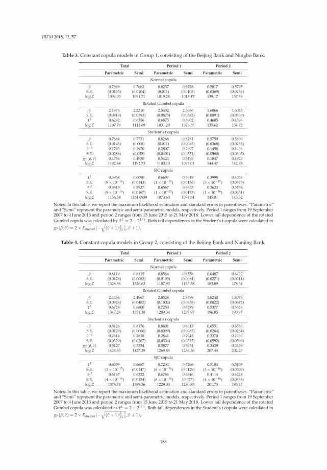
JRFM 2018, 11, 57
Table 3. Constant copula models in Group 1, consisting of the Beijing Bank and Ningbo Bank.
Total Period 1 Period 2
Parametric Semi Parametric Semi Parametric Semi
Normal copula
ρ 0.7669 0.7662 0.8237 0.8228 0.5817 0.5795S.E. (0.0135) (0.0104) (0.011) (0.0108) (0.0369) (0.0266)
logL 1094.03 1091.71 1019.28 1015.47 139.17 137.49
Rotated Gumbel copula
γ 2.1976 2.2310 2.5492 2.5686 1.6066 1.6043S.E. (0.0819) (0.0393) (0.0875) (0.0582) (0.0891) (0.0530)τL 0.6292 0.6356 0.6875 0.6902 0.4605 0.4596
logL 1107.79 1111.69 1031.20 1029.37 135.62 134.72
Student’s t copula
ρ 0.7684 0.7731 0.8268 0.8281 0.5759 0.5800S.E. (0.0145) (0.008) (0.011) (0.0085) (0.0368) (0.0255)ν−1 0.2793 0.2970 0.2807 0.2897 0.1458 0.1496S.E. (0.0286) (0.028) (0.0401) (0.0331) (0.0560) (0.0405)
gT(ρ, ν) 0.4766 0.4930 0.5424 0.5495 0.1847 0.1923logL 1192.44 1192.73 1100.10 1097.01 144.47 142.93
SJC copula
τL 0.5964 0.6090 0.6697 0.6748 0.3998 0.4039S.E. (9 × 10⁻¹⁶) (0.0143) (1 × 10⁻¹⁵) (0.0136) (5 × 10⁻¹⁷) (0.0373)τU 0.5815 0.5937 0.6567 0.6633 0.3623 0.3736S.E. (9 × 10⁻¹⁶) (0.0167) (1 × 10⁻¹⁵) (0.0173) (1 × 10⁻¹⁶) (0.0451)
logL 1156.34 1161.0939 1073.60 1074.64 145.01 143.32
Notes: In this table, we report the maximum likelihood estimation and standard errors in parentheses. “Parametric”and “Semi” represent the parametric and semi-parametric models, respectively. Period 1 ranges from 19 September2007 to 4 June 2015 and period 2 ranges from 15 June 2015 to 21 May 2018. Lower tail dependence of the rotatedGumbel copula was calculated by τL = 2 − 21/γ. Both tail dependences in the Student’s t copula were calculated in
gT(ρ, ν) = 2 × Fstudent(−√(ν + 1) ρ−1
ρ+1 , ν + 1).
Table 4. Constant copula models in Group 2, consisting of the Beijing Bank and Nanjing Bank.
Total Period 1 Period 2
Parametric Semi Parametric Semi Parametric Semi
Normal copula
ρ 0.8119 0.8115 0.8564 0.8556 0.6487 0.6422S.E. (0.0128) (0.0083) (0.0105) (0.0084) (0.0271) (0.0311)
logL 1328.56 1326.63 1187.93 1183.38 183.89 178.64
Rotated Gumbel copula
γ 2.4486 2.4967 2.8528 2.8799 1.8240 1.8076S.E. (0.0926) (0.0482) (0.1002) (0.0638) (0.0822) (0.0673)τL 0.6728 0.6800 0.7250 0.7279 0.5377 0.5326
logL 1347.26 1351.38 1209.54 1207.97 196.85 190.97
Student’s t copula
ρ 0.8126 0.8176 0.8601 0.8613 0.6551 0.6563S.E. (0.0129) (0.0066) (0.0099) (0.0065) (0.0264) (0.0264)ν−1 0.2616 0.2838 0.2841 0.2945 0.2370 0.2393S.E. (0.0329) (0.0267) (0.0334) (0.0325) (0.0592) (0.0500)
gT(ρ, ν) 0.5127 0.5334 0.5877 0.5951 0.3429 0.3459logL 1424.53 1427.29 1269.65 1266.36 207.44 202.25
SJC copula
τL 0.6559 0.6687 0.7204 0.7266 0.5184 0.5109S.E. (1 × 10⁻¹⁵) (0.0147) (8 × 10⁻¹⁶) (0.0129) (5 × 10⁻¹⁶) (0.0305)τU 0.6147 0.6322 0.6786 0.6846 0.4114 0.4228S.E. (4 × 10⁻¹⁶) (0.0154) (8 × 10⁻¹⁶) (0.027) (4 × 10⁻¹⁶) (0.0488)
logL 1378.74 1389.56 1229.00 1230.85 201.73 195.47
Notes: In this table, we report the maximum likelihood estimation and standard errors in parentheses. “Parametric”and “Semi” represent the parametric and semi-parametric models, respectively. Period 1 ranges from 19 September2007 to 4 June 2015 and period 2 ranges from 15 June 2015 to 21 May 2018. Lower tail dependence of the rotatedGumbel copula was calculated as τL = 2 − 21/γ. Both tail dependences in the Student’s t copula were calculated in
gT(ρ, ν) = 2 × Fstudent(−√(ν + 1) ρ−1
ρ+1 , ν + 1).
188
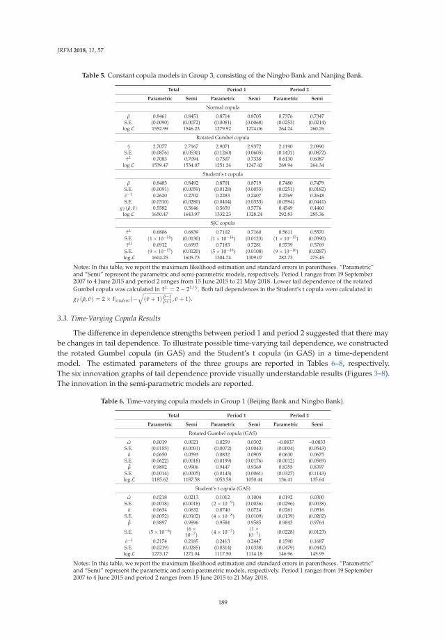
JRFM 2018, 11, 57
Table 5. Constant copula models in Group 3, consisting of the Ningbo Bank and Nanjing Bank.
Total Period 1 Period 2
Parametric Semi Parametric Semi Parametric Semi
Normal copula
ρ 0.8461 0.8451 0.8714 0.8705 0.7376 0.7347S.E. (0.0090) (0.0072) (0.0081) (0.0068) (0.0253) (0.0214)
logL 1552.99 1546.23 1279.92 1274.06 264.24 260.76
Rotated Gumbel copula
γ 2.7077 2.7167 2.9071 2.9372 2.1190 2.0990S.E. (0.0876) (0.0530) (0.1260) (0.0605) (0.1431) (0.0872)τL 0.7083 0.7094 0.7307 0.7338 0.6130 0.6087
logL 1539.47 1534.07 1251.24 1247.42 269.94 264.34
Student’s t copula
ρ 0.8483 0.8492 0.8701 0.8719 0.7480 0.7479S.E. (0.0091) (0.0059) (0.0128) (0.0055) (0.0251) (0.0182)ν−1 0.2620 0.2702 0.2283 0.2407 0.2769 0.2648S.E. (0.0310) (0.0280) (0.0404) (0.0333) (0.0594) (0.0441)
gT(ρ, ν) 0.5582 0.5646 0.5659 0.5776 0.4549 0.4460logL 1650.47 1643.97 1332.23 1328.24 292.83 285.36
SJC copula
τL 0.6806 0.6839 0.7102 0.7160 0.5611 0.5570S.E. (1 × 10⁻¹⁴) (0.0130) (1 × 10⁻¹⁶) (0.0123) (1 × 10⁻¹⁵) (0.0390)τU 0.6912 0.6993 0.7183 0.7281 0.5739 0.5769
S.E. (9 × 10⁻¹⁵) (0.0120) (5 × 10⁻¹⁶) (0.0108) (9 × 10⁻¹⁶) (0.0287)logL 1604.25 1605.73 1304.74 1309.07 282.73 275.45
Notes: In this table, we report the maximum likelihood estimation and standard errors in parentheses. “Parametric”and “Semi” represent the parametric and semi-parametric models, respectively. Period 1 ranges from 19 September2007 to 4 June 2015 and period 2 ranges from 15 June 2015 to 21 May 2018. Lower tail dependence of the rotatedGumbel copula was calculated in τL = 2 − 21/γ. Both tail dependences in the Student’s t copula were calculated in
gT(ρ, ν) = 2 × Fstudent(−√(ν + 1) ρ−1
ρ+1 , ν + 1).
3.3. Time-Varying Copula Results
The difference in dependence strengths between period 1 and period 2 suggested that there maybe changes in tail dependence. To illustrate possible time-varying tail dependence, we constructedthe rotated Gumbel copula (in GAS) and the Student’s t copula (in GAS) in a time-dependentmodel. The estimated parameters of the three groups are reported in Tables 6–8, respectively.The six innovation graphs of tail dependence provide visually understandable results (Figures 3–8).The innovation in the semi-parametric models are reported.
Table 6. Time-varying copula models in Group 1 (Beijing Bank and Ningbo Bank).
Total Period 1 Period 2
Parametric Semi Parametric Semi Parametric Semi
Rotated Gumbel copula (GAS)
ω 0.0019 0.0021 0.0259 0.0302 –0.0837 –0.0833S.E. (0.0155) (0.0001) (0.0072) (0.0043) (0.0004) (0.0543)
α 0.0650 0.0593 0.0832 0.0905 0.0630 0.0675S.E. (0.0622) (0.0018) (0.0199) (0.0176) (0.0012) (0.0569)
β 0.9892 0.9906 0.9447 0.9369 0.8355 0.8397S.E. (0.0014) (0.0005) (0.0143) (0.0061) (0.0327) (0.1143)logL 1185.62 1187.58 1053.58 1050.44 136.41 135.64
Student’s t copula (GAS)
ω 0.0218 0.0213 0.1012 0.1004 0.0192 0.0300S.E. (0.0018) (0.0018) (2 × 10⁻⁹) (0.0036) (0.0296) (0.0038)
α 0.0634 0.0632 0.0740 0.0724 0.0261 0.0516S.E. (0.0052) (0.0102) (4 × 10⁻⁸) (0.0109) (0.0139) (0.0202)
β 0.9897 0.9896 0.9584 0.9585 0.9843 0.9764
S.E. (5 × 10⁻⁶)(6 ×
10−7) (4 × 10⁻⁷)(1 ×
10−7) (0.0228) (0.0123)
ν−1 0.2174 0.2185 0.2413 0.2447 0.1590 0.1687S.E. (0.0219) (0.0285) (0.0314) (0.0338) (0.0479) (0.0442)logL 1273.17 1271.04 1117.50 1114.18 146.96 145.95
Notes: In this table, we report the maximum likelihood estimation and standard errors in parentheses. “Parametric”and “Semi” represent the parametric and semi-parametric models, respectively. Period 1 ranges from 19 September2007 to 4 June 2015 and period 2 ranges from 15 June 2015 to 21 May 2018.
189
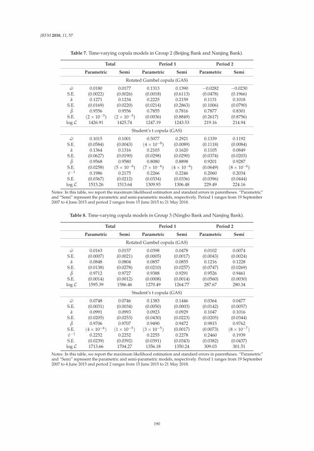
JRFM 2018, 11, 57
Table 7. Time-varying copula models in Group 2 (Beijing Bank and Nanjing Bank).
Total Period 1 Period 2
Parametric Semi Parametric Semi Parametric Semi
Rotated Gumbel copula (GAS)
ω 0.0180 0.0177 0.1313 0.1390 −0.0282 −0.0230S.E. (0.0022) (0.0026) (0.0018) (0.6113) (0.0478) (0.1966)
α 0.1271 0.1234 0.2225 0.2159 0.1131 0.1018S.E. (0.0169) (0.0220) (0.0214) (0.2863) (0.1006) (0.0790)
β 0.9556 0.9556 0.7855 0.7816 0.7877 0.8301S.E. (2 × 10⁻⁵) (2 × 10⁻⁵) (0.0036) (0.8849) (0.2617) (0.8756)logL 1426.91 1425.74 1247.19 1243.53 219.16 214.94
Student’s t copula (GAS)
ω 0.1015 0.1001 0.5077 0.2921 0.1339 0.1192S.E. (0.0584) (0.0043) (4 × 10⁻⁸) (0.0089) (0.1118) (0.0084)
α 0.1364 0.1316 0.2103 0.1620 0.1105 0.0849S.E. (0.0627) (0.0190) (0.0298) (0.0290) (0.0374) (0.0203)
β 0.9568 0.9580 0.8080 0.8898 0.9201 0.9287S.E. (0.0258) (5 × 10⁻⁶) (7 × 10⁻⁶) (4 × 10⁻⁶) (0.0649) (8 × 10⁻⁶)ν−1 0.1986 0.2175 0.2266 0.2246 0.2060 0.2034S.E. (0.0367) (0.0212) (0.0334) (0.0336) (0.0396) (0.0444)logL 1513.26 1513.64 1309.93 1306.48 229.49 224.16
Notes: In this table, we report the maximum likelihood estimation and standard errors in parentheses. “Parametric”and “Semi” represent the parametric and semi-parametric models, respectively. Period 1 ranges from 19 September2007 to 4 June 2015 and period 2 ranges from 15 June 2015 to 21 May 2018.
Table 8. Time-varying copula models in Group 3 (Ningbo Bank and Nanjing Bank).
Total Period 1 Period 2
Parametric Semi Parametric Semi Parametric Semi
Rotated Gumbel copula (GAS)
ω 0.0163 0.0157 0.0398 0.0478 0.0102 0.0074S.E. (0.0007) (0.0021) (0.0005) (0.0017) (0.0043) (0.0024)
α 0.0848 0.0804 0.0857 0.0855 0.1216 0.1228S.E. (0.0138) (0.0278) (0.0210) (0.0257) (0.0747) (0.0269)
β 0.9712 0.9727 0.9388 0.9291 0.9526 0.9461S.E. (0.0014) (0.0012) (0.0008) (0.0014) (0.0560) (0.0030)logL 1595.39 1586.46 1270.49 1264.77 287.67 280.34
Student’s t copula (GAS)
ω 0.0748 0.0746 0.1383 0.1446 0.0364 0.0477S.E. (0.0031) (0.0034) (0.0050) (0.0003) (0.0142) (0.0057)
α 0.0991 0.0993 0.0923 0.0929 0.1047 0.1016S.E. (0.0205) (0.0253) (0.0430) (0.0223) (0.0205) (0.0344)
β 0.9706 0.9707 0.9490 0.9472 0.9815 0.9762S.E. (4 × 10⁻⁶) (1 × 10⁻⁵) (3 × 10⁻⁵) (0.0017) (0.0073) (8 × 10⁻⁷)ν−1 0.2252 0.2252 0.2255 0.2278 0.2460 0.1939S.E. (0.0239) (0.0392) (0.0391) (0.0343) (0.0382) (0.0437)logL 1713.66 1704.27 1356.18 1350.24 309.03 301.51
Notes: In this table, we report the maximum likelihood estimation and standard errors in parentheses. “Parametric”and “Semi” represent the parametric and semi-parametric models, respectively. Period 1 ranges from 19 September2007 to 4 June 2015 and period 2 ranges from 15 June 2015 to 21 May 2018.
190
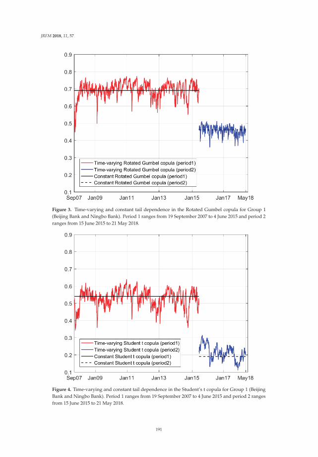
JRFM 2018, 11, 57
Figure 3. Time-varying and constant tail dependence in the Rotated Gumbel copula for Group 1(Beijing Bank and Ningbo Bank). Period 1 ranges from 19 September 2007 to 4 June 2015 and period 2ranges from 15 June 2015 to 21 May 2018.
Figure 4. Time-varying and constant tail dependence in the Student’s t copula for Group 1 (BeijingBank and Ningbo Bank). Period 1 ranges from 19 September 2007 to 4 June 2015 and period 2 rangesfrom 15 June 2015 to 21 May 2018.
191
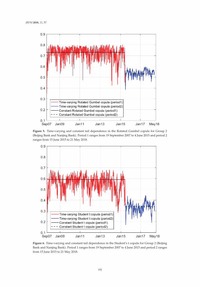
JRFM 2018, 11, 57
Figure 5. Time-varying and constant tail dependence in the Rotated Gumbel copula for Group 2(Beijing Bank and Nanjing Bank). Period 1 ranges from 19 September 2007 to 4 June 2015 and period 2ranges from 15 June 2015 to 21 May 2018.
Figure 6. Time-varying and constant tail dependence in the Student’s t copula for Group 2 (BeijingBank and Nanjing Bank). Period 1 ranges from 19 September 2007 to 4 June 2015 and period 2 rangesfrom 15 June 2015 to 21 May 2018.
192
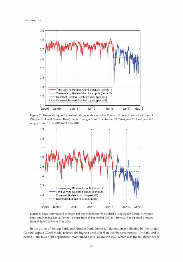
JRFM 2018, 11, 57
Figure 7. Time-varying and constant tail dependence in the Rotated Gumbel copula for Group 3(Ningbo Bank and Nanjing Bank). Period 1 ranges from 19 September 2007 to 4 June 2015 and period 2ranges from 15 June 2015 to 21 May 2018.
Figure 8. Time-varying and constant tail dependence in the Student’s t copula for Group 3 (NingboBank and Nanjing Bank). Period 1 ranges from 19 September 2007 to 4 June 2015 and period 2 rangesfrom 15 June 2015 to 21 May 2018.
In the group of Beijing Bank and Ningbo Bank, lower tail dependence indicated by the rotatedGumbel copula (GAS) model reached the highest level of 0.75 in less than six months. Until the end ofperiod 1, the lower tail dependence maintained a level at around 0.69, which was the tail dependence
193
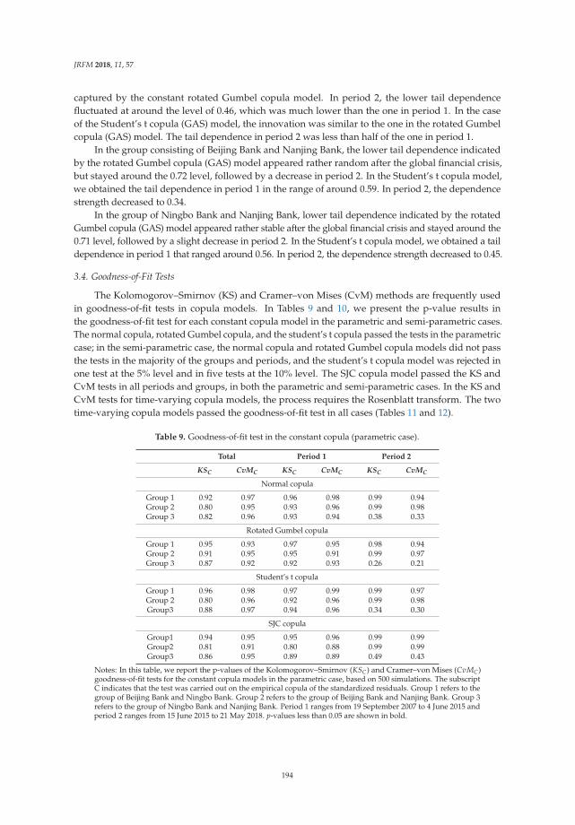
JRFM 2018, 11, 57
captured by the constant rotated Gumbel copula model. In period 2, the lower tail dependencefluctuated at around the level of 0.46, which was much lower than the one in period 1. In the caseof the Student’s t copula (GAS) model, the innovation was similar to the one in the rotated Gumbelcopula (GAS) model. The tail dependence in period 2 was less than half of the one in period 1.
In the group consisting of Beijing Bank and Nanjing Bank, the lower tail dependence indicatedby the rotated Gumbel copula (GAS) model appeared rather random after the global financial crisis,but stayed around the 0.72 level, followed by a decrease in period 2. In the Student’s t copula model,we obtained the tail dependence in period 1 in the range of around 0.59. In period 2, the dependencestrength decreased to 0.34.
In the group of Ningbo Bank and Nanjing Bank, lower tail dependence indicated by the rotatedGumbel copula (GAS) model appeared rather stable after the global financial crisis and stayed around the0.71 level, followed by a slight decrease in period 2. In the Student’s t copula model, we obtained a taildependence in period 1 that ranged around 0.56. In period 2, the dependence strength decreased to 0.45.
3.4. Goodness-of-Fit Tests
The Kolomogorov–Smirnov (KS) and Cramer–von Mises (CvM) methods are frequently usedin goodness-of-fit tests in copula models. In Tables 9 and 10, we present the p-value results inthe goodness-of-fit test for each constant copula model in the parametric and semi-parametric cases.The normal copula, rotated Gumbel copula, and the student’s t copula passed the tests in the parametriccase; in the semi-parametric case, the normal copula and rotated Gumbel copula models did not passthe tests in the majority of the groups and periods, and the student’s t copula model was rejected inone test at the 5% level and in five tests at the 10% level. The SJC copula model passed the KS andCvM tests in all periods and groups, in both the parametric and semi-parametric cases. In the KS andCvM tests for time-varying copula models, the process requires the Rosenblatt transform. The twotime-varying copula models passed the goodness-of-fit test in all cases (Tables 11 and 12).
Table 9. Goodness-of-fit test in the constant copula (parametric case).
Total Period 1 Period 2
KSC CvMC KSC CvMC KSC CvMC
Normal copula
Group 1 0.92 0.97 0.96 0.98 0.99 0.94Group 2 0.80 0.95 0.93 0.96 0.99 0.98Group 3 0.82 0.96 0.93 0.94 0.38 0.33
Rotated Gumbel copula
Group 1 0.95 0.93 0.97 0.95 0.98 0.94Group 2 0.91 0.95 0.95 0.91 0.99 0.97Group 3 0.87 0.92 0.92 0.93 0.26 0.21
Student’s t copula
Group 1 0.96 0.98 0.97 0.99 0.99 0.97Group 2 0.80 0.96 0.92 0.96 0.99 0.98Group3 0.88 0.97 0.94 0.96 0.34 0.30
SJC copula
Group1 0.94 0.95 0.95 0.96 0.99 0.99Group2 0.81 0.91 0.80 0.88 0.99 0.99Group3 0.86 0.95 0.89 0.89 0.49 0.43
Notes: In this table, we report the p-values of the Kolomogorov–Smirnov (KSC) and Cramer–von Mises (CvMC)goodness-of-fit tests for the constant copula models in the parametric case, based on 500 simulations. The subscriptC indicates that the test was carried out on the empirical copula of the standardized residuals. Group 1 refers to thegroup of Beijing Bank and Ningbo Bank. Group 2 refers to the group of Beijing Bank and Nanjing Bank. Group 3refers to the group of Ningbo Bank and Nanjing Bank. Period 1 ranges from 19 September 2007 to 4 June 2015 andperiod 2 ranges from 15 June 2015 to 21 May 2018. p-values less than 0.05 are shown in bold.
194
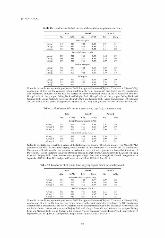
JRFM 2018, 11, 57
Table 10. Goodness-of-fit test in constant copula (semi-parametric case).
Total Period 1 Period 2
KSC CvMC KSC CvMC KSC CvMC
Normal copula
Group1 0.17 0.01 0.14 0.00 0.91 0.61Group2 0.09 0.01 0.02 0.00 0.22 0.24Group3 0.07 0.01 0.09 0.04 0.15 0.02
Rotated Gumbel copula
Group1 0.00 0.00 0.00 0.00 0.12 0.00Group2 0.00 0.00 0.00 0.00 0.13 0.00Group3 0.00 0.00 0.00 0.00 0.00 0.00
Student’s t copula
Group1 0.62 0.54 0.04 0.10 0.88 0.70Group2 0.48 0.50 0.05 0.07 0.58 0.63Group3 0.17 0.29 0.44 0.23 0.50 0.10
SJC copula
Group1 0.99 0.99 0.99 0.99 0.99 0.99Group2 0.99 0.99 0.99 0.99 0.99 0.99Group3 0.99 0.99 0.99 0.99 0.99 0.99
Notes: In this table, we report the p-values of the Kolomogorov–Smirnov (KSC) and Cramer–von Mises (CvMC)goodness-of-fit tests for the constant copula models in the semi-parametric case, based on 500 simulations.The subscript C indicates that the test was carried out on the empirical copula of the standardized residuals.Group 1 refers to the group of Beijing Bank and Ningbo Bank. Group 2 refers to the group of Beijing Bank andNanjing Bank. Group 3 refers to the group of Ningbo Bank and Nanjing Bank. Period 1 ranges from 19 September2007 to 4 June 2015 and period 2 ranges from 15 June 2015 to 21 May 2018. p-values less than 0.05 are shown in bold.
Table 11. Goodness-of-fit test in time-varying copula (parametric case).
Total Period 1 Period 2
KSR CvMR KSR CvMR KSR CvMR
Rotated Gumbel copula (GAS)
Group 1 0.99 0.99 0.99 0.99 0.97 0.96Group 2 0.99 0.99 0.99 0.88 0.99 0.99Group 3 0.99 0.99 0.97 0.97 0.80 0.69
Student’s t copula (GAS)
Group 1 0.99 0.99 0.99 0.99 0.99 0.99Group 2 0.99 0.99 0.98 0.99 0.99 0.99Group 3 0.99 0.99 0.96 0.97 0.92 0.81
Notes: In this table, we report the p-values of the Kolomogorov–Smirnov (KSR) and Cramer–von Mises (CvMR)goodness-of-fit tests for the time-varying copula models in the parametric case, based on 100 simulations.The subscript R indicates that the test was carried out on the empirical copula of the Rosenblatt transform ofthe residuals. Group 1 refers to the group of Beijing Bank and Ningbo Bank. Group 2 refers to the group of BeijingBank and Nanjing Bank. Group 3 refers to the group of Ningbo Bank and Nanjing Bank. Period 1 ranges from 19September 2007 to 4 June 2015 and period 2 ranges from 15 June 2015 to 21 May 2018.
Table 12. Goodness-of-fit test in time-varying copula (semi-parametric case).
Total Period 1 Period 2
KSR CvMR KSR CvMR KSR CvMR
Rotated Gumbel copula (GAS)Group 1 0.81 0.99 0.24 0.97 0.09 0.33Group 2 0.83 0.99 0.98 0.99 0.47 0.44Group 3 0.85 0.99 0.93 0.99 0.93 0.88
Student’s t copula (GAS)
Group 1 0.63 0.59 0.39 0.40 0.66 0.57Group 2 0.99 0.89 0.66 0.67 0.96 0.96Group 3 0.58 0.80 0.50 0.60 0.61 0.62
Notes: In this table, we report the p-values of the Kolomogorov–Smirnov (KSR) and Cramer–von Mises (CvMR)goodness-of-fit tests for the time-varying copula models in the semi-parametric case, based on 100 simulations.The subscript R indicates that the test was carried out on the empirical copula of the Rosenblatt transform of theresiduals. Group 1 refers to the group of Beijing Bank and Ningbo Bank. Group 2 refers to the group of BeijingBank and Nanjing Bank. Group 3 refers to the group of Ningbo Bank and Nanjing Bank. Period 1 ranges from 19September 2007 to 4 June 2015 and period 2 ranges from 15 June 2015 to 21 May 2018.
195
JRFM 2018, 11, 57
4. Conclusions
In this study on the share price returns of three city banks, we investigated the potentialdependence structure. We used copula models rather than the usual linear correlation to capture thedetailed tail dependence. We used various copula models to estimate the underlying dependencein extreme periods. The Student’s t, SJC, and rotated Gumbel copula models could specify the taildependence with higher log-likelihood values better than the other copula models. Furthermore,by extending the Student’s t and rotated Gumbel copula models to the GAS and time-varying models,we could obtain more information about the innovation of changes in tail dependence.
Unlike most of the literature using copula models, we focused on the tail dependence of theshare price returns of city banks rather than aggregate variables, such as share markets indices andexchange rates. The tail dependence may be dependent on profitability, own risks, inter-bank business,and outside influence. Although city banks fall in the same sector in share markets, they may havediverse returns due to different strategies or business behaviors. During and after a stock marketcrash, the city banks may have diverse reactions, which supports our assumption that there may be adifferent level of dependence between two banks during two periods.
We found diverse dependence structures among the three groups of city banks. First, the taildependence was higher between the share price returns of Ningbo Bank and Nanjing Bank, than that ofthe other two combinations. Beijing Bank was less dependent on the other two city banks, and NanjingBank was dependent on the other two. Ningbo Bank was more dependent on Nanjing Bank, than onBeijing Bank. Second, we observed a major break in the three dependence structures. Beijing Bankbecame much less dependent on the other two banks during the 2015 domestic share market crash,than during the 2008 financial crisis. However, the dependency of Nanjing Bank on Ningbo Bank didnot change as much as that of the other two combinations from 2008 to 2015. Third, the share prices ofNingbo Bank and Nanjing Bank had a slightly higher possibility of increasing than decreasing together.This was different from recent studies on financial asset price co-movement, which often suggest thatfinancial assets tend to have more dependence in price crashes than in booms.
The share price returns of Ningbo Bank were found to be more similar to that of Nanjing Bank,compared to that of Beijing Bank. This observation of the share price extreme returns of three citybanks reconfirmed our research results in the copula models. Risk-avoiding behavior is a possiblecause of the decrease in tail dependence. It is recommended that for city commercial banks, strategiessuch as obtaining superior assets and involving less risky inter-bank business be adopted, and that forthe central bank, reasonable capital liquidity and supervision should be ensured to create a healthierinter-bank market. Nowadays, the majority of local Chinese companies are experiencing low profitmargins. The central and local governments should help boost the domestic economy, under bothfiscal and monetary policies, and avoid the crisis from happening in the real economy, which maytransmit to banking systems.
Author Contributions: S.H. conceived and designed the experiments; G.L. performed the experiments, analyzedthe data, and contributed reagents/materials/analysis tools; G.L., X.-J.C., and S.H. wrote the paper.
Funding: This research was funded by JSPS KAKENHI Grant Number 17K18564 and (A) 17H00983.
Acknowledgments: We are grateful to three anonymous referees for their helpful comments and suggestions.We are also grateful to the participants of The SIBR 2018 Hong Kong Conference on Interdisciplinary Business &Economics Research for helpful comments.
Conflicts of Interest: The authors declare no conflict of interest. The founding sponsors had no role in the designof the study, in the collection, analyses, or interpretation of data, in the writing of the manuscript, or in the decisionto publish the results.
References
Ang, Andrew, and Joseph Chen. 2002. Asymmetric correlations of equity portfolios. Journal of Financial Economics63: 443–94. [CrossRef]
196

JRFM 2018, 11, 57
Bollerslev, Tim. 1987. A conditionally heteroskedastic time series model for speculative prices and rates of return.The Review of Economics and Statistics 69: 542–47. [CrossRef]
Casella, G., and Roger L. Berger. 1990. Statistical Inference. Belmont: Duxbury Press.Creal, D., Siem Jan Koopman, and André Lucas. 2013. Generalized autoregressive score models with applications.
Journal of Applied Econometrics 28: 777–95. [CrossRef]Fama, Eugene F. 1965. The behavior of stock-market prices. The Journal of Business 38: 34–105. [CrossRef]Gumbel, Emil J. 1960. Bivariate exponential distributions. Journal of the American Statistical Association 55: 698–707.
[CrossRef]Hansen, Bruce E. 1994. Autoregressive conditional density estimation. International Economic Review, 705–30.
[CrossRef]Joe, Harry. 1997. Multivariate Models and Multivariate Dependence Concepts. Boca Raton: CRC Press.Luo, W., Robert D. Brooks, and Param Silvapulle. 2011. Effects of the open policy on the dependence between the
Chinese ‘A’ stock market and other equity markets: An industry sector perspective. Journal of InternationalFinancial Markets, Institutions and Money 21: 49–74. [CrossRef]
Marimoutou, Vêlayoudom, and Manel Soury. 2015. Energy markets and CO2 emissions: Analysis by stochasticcopula autoregressive model. Energy 88: 417–29. [CrossRef]
Patton, Andrew J. 2006. Modelling asymmetric exchange rate dependence. International Economic Review 47:527–56. [CrossRef]
Patton, Andrew J. 2013. Copula methods for forecasting multivariate time series. In Handbook of EconomicForecasting. New York: Elsevier, vol. 2, pp. 899–960. [CrossRef]
Reboredo, Juan C., and Andrea Ugolini. 2015. Downside/upside price spillovers between precious metals: A vinecopula approach. The North American Journal of Economics and Finance 34: 84–102. [CrossRef]
Sklar, Abe. 1959. Fonctions de répartition à n dimensions et leurs marges. Publications de l’Institut de Statistique del’Université de Paris 8: 229–31.
Sukcharoen, Kunlapath, Tatevik Zohrabyan, David Leatham, and Ximing Wu. 2014. Interdependence of oil pricesand stock market indices: A copula approach. Energy Economics 44: 331–39. [CrossRef]
© 2018 by the authors. Licensee MDPI, Basel, Switzerland. This article is an open accessarticle distributed under the terms and conditions of the Creative Commons Attribution(CC BY) license (http://creativecommons.org/licenses/by/4.0/).
197
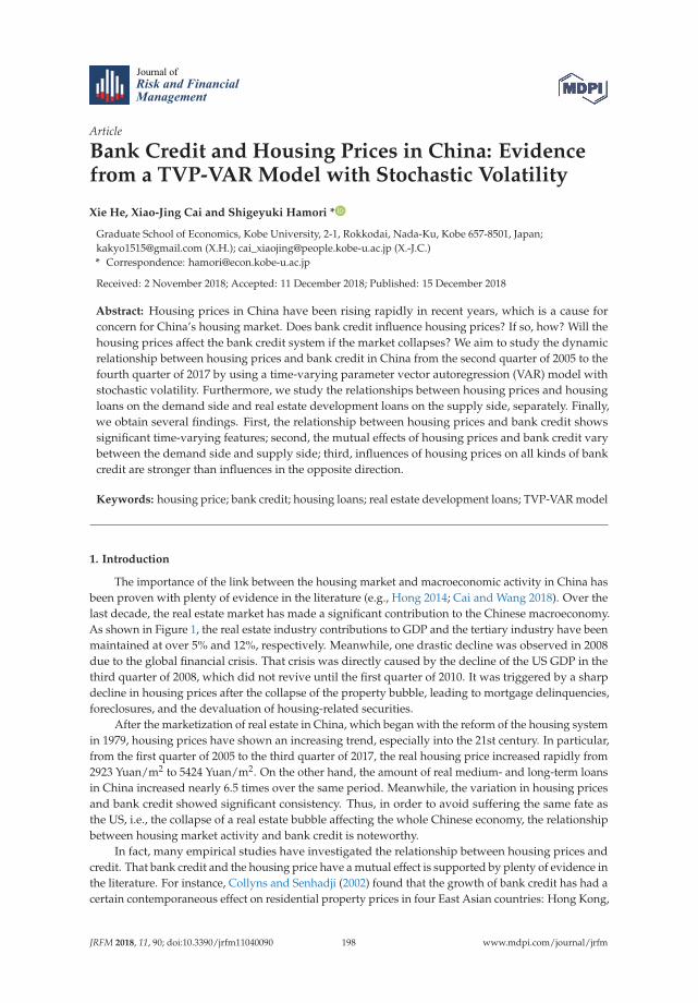
Journal of
Risk and FinancialManagement
Article
Bank Credit and Housing Prices in China: Evidencefrom a TVP-VAR Model with Stochastic Volatility
Xie He, Xiao-Jing Cai and Shigeyuki Hamori *
Graduate School of Economics, Kobe University, 2-1, Rokkodai, Nada-Ku, Kobe 657-8501, Japan;[email protected] (X.H.); [email protected] (X.-J.C.)* Correspondence: [email protected]
Received: 2 November 2018; Accepted: 11 December 2018; Published: 15 December 2018
Abstract: Housing prices in China have been rising rapidly in recent years, which is a cause forconcern for China’s housing market. Does bank credit influence housing prices? If so, how? Will thehousing prices affect the bank credit system if the market collapses? We aim to study the dynamicrelationship between housing prices and bank credit in China from the second quarter of 2005 to thefourth quarter of 2017 by using a time-varying parameter vector autoregression (VAR) model withstochastic volatility. Furthermore, we study the relationships between housing prices and housingloans on the demand side and real estate development loans on the supply side, separately. Finally,we obtain several findings. First, the relationship between housing prices and bank credit showssignificant time-varying features; second, the mutual effects of housing prices and bank credit varybetween the demand side and supply side; third, influences of housing prices on all kinds of bankcredit are stronger than influences in the opposite direction.
Keywords: housing price; bank credit; housing loans; real estate development loans; TVP-VAR model
1. Introduction
The importance of the link between the housing market and macroeconomic activity in China hasbeen proven with plenty of evidence in the literature (e.g., Hong 2014; Cai and Wang 2018). Over thelast decade, the real estate market has made a significant contribution to the Chinese macroeconomy.As shown in Figure 1, the real estate industry contributions to GDP and the tertiary industry have beenmaintained at over 5% and 12%, respectively. Meanwhile, one drastic decline was observed in 2008due to the global financial crisis. That crisis was directly caused by the decline of the US GDP in thethird quarter of 2008, which did not revive until the first quarter of 2010. It was triggered by a sharpdecline in housing prices after the collapse of the property bubble, leading to mortgage delinquencies,foreclosures, and the devaluation of housing-related securities.
After the marketization of real estate in China, which began with the reform of the housing systemin 1979, housing prices have shown an increasing trend, especially into the 21st century. In particular,from the first quarter of 2005 to the third quarter of 2017, the real housing price increased rapidly from2923 Yuan/m2 to 5424 Yuan/m2. On the other hand, the amount of real medium- and long-term loansin China increased nearly 6.5 times over the same period. Meanwhile, the variation in housing pricesand bank credit showed significant consistency. Thus, in order to avoid suffering the same fate asthe US, i.e., the collapse of a real estate bubble affecting the whole Chinese economy, the relationshipbetween housing market activity and bank credit is noteworthy.
In fact, many empirical studies have investigated the relationship between housing prices andcredit. That bank credit and the housing price have a mutual effect is supported by plenty of evidence inthe literature. For instance, Collyns and Senhadji (2002) found that the growth of bank credit has had acertain contemporaneous effect on residential property prices in four East Asian countries: Hong Kong,
JRFM 2018, 11, 90; doi:10.3390/jrfm11040090 www.mdpi.com/journal/jrfm198

JRFM 2018, 11, 90
Korea, Singapore, and Thailand. They concluded that bank lending contributed significantly to thereal estate bubble in Asia prior to the 1997 East Asian crisis. The findings of Mora (2008) prove thatbank lending is a possible explanation for the Japanese real estate boom during the 1980s. Gimeno andCarrascal (2010) found that credit had a positive causality on the housing price in Spain when the creditaggregate departed from its long-run level. Gerlach and Peng (2005) examined the relationship betweenproperty prices and bank lending in Hong Kong, and their results suggest that the development ofproperty prices influences bank lending.1
0
1,000
2,000
3,000
4,000
5,000
6,000
0%
2%
4%
6%
8%
10%
12%
14%
2005 2006 2007 2008 2009 2010 2011 2012 2013 2014 2015 2016Real estate industry
The proportion of real estate industry to GDP
The proportion of real estate industry to tertiary industry
Billion Yuan
Figure 1. The Chinese real estate industry contributions to the tertiary industry and GDP in billions ofYuan. Source: China Statistics Bureau.
Davis and Zhu (2011) argued that the effect of commercial property prices on credit is strongerthan the reverse. More importantly, their research showed that because bank credit affects both theproperty buyer and the developer, when bank credit is extended, it may boost demand and stimulate anincrease in housing prices. Credit has a positive effect on commercial property prices in the short run.Meanwhile, the extension of bank credit may also finance new construction, and housing prices willfinally adjust downwards through an improvement in supply. However, because of the lags in supply,the negative effect will only be felt in the long term.
Based on this perspective, this study makes two contributions. First, we not only observe therelationship between the housing price and bank credit in market as a whole but also divide themarket into two parts: the demand side and the supply side. We intend to quantify the differentrelationships between housing prices and bank credit on these two fronts. Hence, this paper comparesthree different variable sets from the market as a whole, and from the demand and supply sides of thehousing market.
The second contribution is that unlike most previous studies which were based on the simplevector autoregression (VAR) model, we adopt the time-varying parameter VAR (TVP-VAR) modelwith stochastic volatility which delivers more accurate empirical results. The simple VAR modelhas an obvious limitation: linear coefficients are time-invariant. However, in reality, the economicstructure and the relationships among economic variables are more complicated and change over time,which means that the linear and time-invariant features of a simple VAR model are unrealistic.
1 Yuan and Hamori (2014) analyzed the crowding out effect of affordable and unaffordable housing in China.
199
JRFM 2018, 11, 90
However, the TVP-VAR model can circumvent this problem perfectly. As stated by Nakajima (2011),“The TVP-VAR model enables us to capture the possible time-varying nature of the underlying structurein the economy in a flexible and robust manner”. Moreover, stochastic volatility, which also influencesthe data generating process of economic variables and was originally proposed by Black (1976),may cause misspecification if it is ignored during analysis. Nakajima (2011) estimated the TVPregression model with stochastic volatility and constant volatility for a given set of simulated data,finding that the estimation result of the model with stochastic volatility was closer to the true value.Tian and Hamori (2016) use a time-varying structural vector auto-regression model with stochasticvolatility to study the financial shock transmission mechanism. For this reason, we also incorporatestochastic volatility into the TVP-VAR model. On the other hand, due to the intractability of thelikelihood function, stochastic volatility makes the estimation difficult. To circumvent this problem,we also use Markov chain Monte Carlo (MCMC) methods in the context of a Bayesian inference toestimate the model.
In this paper, our empirical results are presented in three parts. First, we find that the relationshipbetween housing prices and bank credit has significant time-varying features. Second, the mutualeffect between housing prices and bank credit varies on both the demand side and the supply side.Third, the influences of housing prices on all kinds of bank credit are stronger than influences in theopposite direction.
The remainder of the article is organized as follows. Section 2 presents a theoretical analysis ofthe interaction effect between bank credit and housing prices based on references. Section 3 introducesthe model specifications. Section 4 discusses the data and the identification procedure. Section 5 showsthe empirical results of each set of variables, and Section 6 presents the conclusions.
2. Theoretical Analysis of the Interaction Effect between Bank Credit and Housing Prices
Bank credit is considered to influence the housing market. Although bank credit is consideredto have a positive effect on housing prices in general, in fact, the effect should not be understood asa whole, as it not only depends on the objects of bank credit—both the supply side of housing andthe demand side—but it also depends on time. The effect of bank credit on housing prices may differbecause of differences in influences on the two sides of the housing market. In addition, the differentperiods and lengths of time will also change the effect.
On the demand side, there is no doubt that housing loans are the main way for general consumersto buy houses. As housing loans expand, the demand for housing will also increase. This demand is notonly for personal use but also for investment. In China, property is considered to be a good investmentdue to its ability to increase in value. Once housing loans can be obtained easily, speculative demandfor property can also be stimulated with the help of bank funds, especially in the short term, because thesupply of housing is inelastic, so prices will increase as a result of influences from the demand side.
On the supply side, the long-term and the short-term effects of real estate development loan2 onhousing prices are different. In China, real estate development loans are the main source of capitalfor constructors. According to calculations by Qin and Yao (2012), from 1998 to 2010, the averageannual proportion of capital gained directly by banks from real estate development investment wasmore than 20.78%, while if the capital gained indirectly by banks, such as from down payments andpersonal mortgages, is also counted3, this proportion is more than 66.81%. Thus, it is not difficult to seehow important bank credit is to the constructors. In fact, since the marketization of real estate in China,the housing market in China has always been a seller’s market in which the constructors have morebargaining power than the buyers. Meanwhile, in the short term, bank credit can relieve the financial
2 In this paper, real estate development loan refers to the loan that bank issues to the borrower to finance construction of realestates and supportive facilities.
3 In China, the presale of commercial residential houses allows developers to use the capital that consumers borrow from thebank for construction.
200
JRFM 2018, 11, 90
pressure of constructors, further enhancing their bargaining power and pushing up housing prices.However, in the long term, high real estate development also leads to a high supply of housing,and after the 2008 financial crisis, a high investment in the housing market led to a “high inventory”problem in China. In October 2016, the number of residential houses for sale hit another historical high.Many cities in China that have a high inventory of housing face huge pressure to reduce their numbersof unsold homes. Thus, high real estate loans will also make housing prices decrease in the long termbecause of oversupply in the long term, as concluded by Davis and Zhu (2011).
On the other hand, the growth of housing prices also has a strong effect on bank credit. In periodswhen housing prices continue to rise, banks are likely to underestimate the risk of credit on real estatedevelopment, causing them to expand their credit supply to the real estate industry.
For general consumers, based on research by Goodhart and Hofmann (2008) and other references,the growth of housing prices will mainly affect housing loans in three ways: the wealth effect,the collateral effect, and the expectation effect. First, the growth of housing prices via the wealth effectmakes individuals willing to get more credit from the bank. Under the life cycle model of householdconsumption, a permanent increase in housing wealth can increase both household spending andborrowing if individuals want to smooth consumption over their life cycles. Second, since property is ageneral collateral item, a growth in housing prices can also increase the collateral value of individualswhich can lead to lenders getting credit from the bank more easily. Third, the expectation effectexplains that if housing prices begin to rise, consumers will anticipate that they will keep increasing,which encourages them to get a bigger housing loan to purchase property as soon as possible.
For the constructors, rises in housing prices can increase their expected investment return inreal estate development, which will inevitably encourage them to expand their investment scale andattract new companies to enter the field. Since bank credit is the most important source of capital forthe constructors, credit demand will significantly increase.
3. Time-Varying Parameter VAR Model with Stochastic Volatility
This paper follows Nakajima (2011) for the time-varying TVP-VAR model with stochasticvolatility4. Consider the time varying structural VAR model
Atyt = B0t + B1tyt−1 + · · ·+ Bstyt−s + ut, t = s + 1, . . . n, (1)
where yt is a k × 1 vector of observed variables, B0t is an k × 1 vector of the intercept term,At, ct, B1t, . . . , Bst are k × k matrices of time varying coefficients. The disturbance ut is a k × 1time-varying structural shock, and it is assumed that ut ∼ N(0, ∑t ∑t), where
∑t=
⎛⎜⎜⎜⎜⎜⎝σ1,t 0 · · · 0
0 σ2,t. . .
......
. . . . . . 00 · · · 0 σk,t
⎞⎟⎟⎟⎟⎟⎠The simultaneous relations of the structural shock are specified by recursive identification,
assuming that At is lower-triangular. Meanwhile, it is important to note that At is allowed to varyover time, which implies that an innovation to the i-th variable has a time invariant effect on thej-th variable:
4 Hereafter, for simplicity, we use the “TVP-VAR model” to indicate the model with stochastic volatility.
201
JRFM 2018, 11, 90
At =
⎛⎜⎜⎜⎜⎜⎝1 0 · · · 0
a21,t. . . . . .
......
. . . . . . 0ak1,t · · · akk−1,t 1
⎞⎟⎟⎟⎟⎟⎠Thus, Equation (1) can be rewritten as the following reduced form VAR model:
yt = C0t + C1tyt−1 + · · ·+ Cstyt−s + A−1t ∑
tεt, εt ∼ N(0, Ik), (2)
where Cit = A−1t Bit, for i = 0, . . . , s. By stacking the elements in the rows of Ci’s to a vector ςt
(k2(s + 1)× 1 vector), the model can be written as follows:
yt = Xtςt + A−1t ∑
tεt. (3)
Xt = Ik ⊗(1, y′t−1, · · · , y′t−s
), t = s + 1, · · · , n
where ⊗ denotes the Kronecker product. Meanwhile, following Primiceri (2005), at =
(a21, a31, a32, a41, · · · , ak,k−1)′ is a stacked vector of the lower-triangular elements, assuming ςt,
At, and ∑t all change over time.If the variance is assumed to be constant while the coefficients are time-varying, it will cause
the estimate parameters to be biased, because the possibility of volatility variation is ignored(Nakajima, 2011). To avoid this misspecification, stochastic volatility is also incorporated into theTVP-VAR model. It is assumed that the log-volatility is ht = (h1t, · · · , hkt)
′, hjt = log σ2jt, and for
j = 1, · · · , k, t = s + 1, . . . , n, it is also modeled to follow a random walk. The variances (σ2jt)
are assumed to evolve as geometric random walks belonging to the class of models known asstochastic volatility.5
The dynamics of the model’s time varying parameters in (3) and the stochastic volatility arespecified as follows:
ςt+1 = ςt + uςt,
at+1 = at + uat,
ht+1 = ht + uht,
⎛⎜⎜⎜⎝εt
uςt
uat
uht
⎞⎟⎟⎟⎠ ∼ N
⎛⎜⎜⎜⎝0,
⎛⎜⎜⎜⎝I O O OO ∑ς O OO O ∑a OO O O ∑h
⎞⎟⎟⎟⎠⎞⎟⎟⎟⎠, (4)
for t = s + 1, · · · , n, where ςs+1 ∼ N(μς0 , ∑ς0
), as+1 ∼ N
(μa0 , ∑a0
)and hs+1 ∼ N
(μh0 , ∑h0
).
Moreover, in this paper, we also make two assumptions that follow Nakajima (2011) and need tobe stated. First, the assumption of a lower-triangular matrix for At is the recursive identification forthe VAR system. Second, for simplicity, we assume that ∑a and ∑h are diagonal matrices.
4. Data and Settings
Table 1 shows all variables in our model. In out paper we use a four-variable TVP-VAR modelto estimate the quarterly seasonally-adjusted data from the second quarter of 2005 to the fourthquarter of 2017 in China6. Furthermore, we estimated three different sets of variables. The first setwas defined as yt = (IRt, GDPt, BCt, HPt), the second is yt = (IRt, GDPt, HLt, HPt), and the third is
5 Here, we use the log-normal SV model, which was originally proposed by Taylor (1986). The simplest model can also be
defined: yt = γ exp(
ht2
), ht+1 = φht + ηt, ηt ∼ NID
(0, σ2
η
), t = 0, . . . , n − 1, γ > 0. For more details on the statistical
aspects of ARCH and stochastic volatility, see Shephard (1996). Yang and Hamori (2018) compared the performances of theGARCH and SV models to analyze international agricultural commodity prices.
6 Because of the availability of data, we started the sample period in the second quarter of 2005.
202
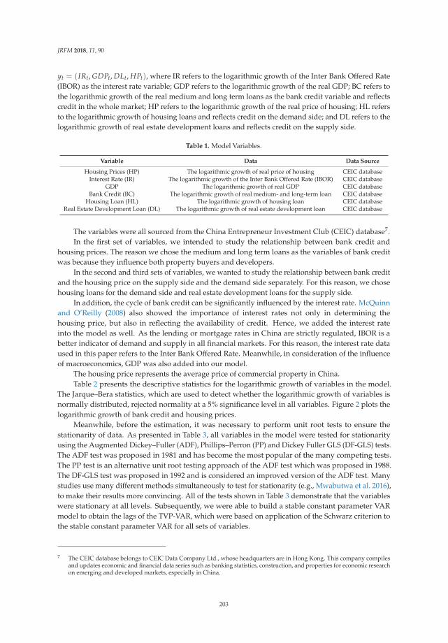
JRFM 2018, 11, 90
yt = (IRt, GDPt, DLt, HPt), where IR refers to the logarithmic growth of the Inter Bank Offered Rate(IBOR) as the interest rate variable; GDP refers to the logarithmic growth of the real GDP; BC refers tothe logarithmic growth of the real medium and long term loans as the bank credit variable and reflectscredit in the whole market; HP refers to the logarithmic growth of the real price of housing; HL refersto the logarithmic growth of housing loans and reflects credit on the demand side; and DL refers to thelogarithmic growth of real estate development loans and reflects credit on the supply side.
Table 1. Model Variables.
Variable Data Data Source
Housing Prices (HP) The logarithmic growth of real price of housing CEIC databaseInterest Rate (IR) The logarithmic growth of the Inter Bank Offered Rate (IBOR) CEIC database
GDP The logarithmic growth of real GDP CEIC databaseBank Credit (BC) The logarithmic growth of real medium- and long-term loan CEIC database
Housing Loan (HL) The logarithmic growth of housing loan CEIC databaseReal Estate Development Loan (DL) The logarithmic growth of real estate development loan CEIC database
The variables were all sourced from the China Entrepreneur Investment Club (CEIC) database7.In the first set of variables, we intended to study the relationship between bank credit and
housing prices. The reason we chose the medium and long term loans as the variables of bank creditwas because they influence both property buyers and developers.
In the second and third sets of variables, we wanted to study the relationship between bank creditand the housing price on the supply side and the demand side separately. For this reason, we chosehousing loans for the demand side and real estate development loans for the supply side.
In addition, the cycle of bank credit can be significantly influenced by the interest rate. McQuinnand O’Reilly (2008) also showed the importance of interest rates not only in determining thehousing price, but also in reflecting the availability of credit. Hence, we added the interest rateinto the model as well. As the lending or mortgage rates in China are strictly regulated, IBOR is abetter indicator of demand and supply in all financial markets. For this reason, the interest rate dataused in this paper refers to the Inter Bank Offered Rate. Meanwhile, in consideration of the influenceof macroeconomics, GDP was also added into our model.
The housing price represents the average price of commercial property in China.Table 2 presents the descriptive statistics for the logarithmic growth of variables in the model.
The Jarque–Bera statistics, which are used to detect whether the logarithmic growth of variables isnormally distributed, rejected normality at a 5% significance level in all variables. Figure 2 plots thelogarithmic growth of bank credit and housing prices.
Meanwhile, before the estimation, it was necessary to perform unit root tests to ensure thestationarity of data. As presented in Table 3, all variables in the model were tested for stationarityusing the Augmented Dickey–Fuller (ADF), Phillips–Perron (PP) and Dickey Fuller GLS (DF-GLS) tests.The ADF test was proposed in 1981 and has become the most popular of the many competing tests.The PP test is an alternative unit root testing approach of the ADF test which was proposed in 1988.The DF-GLS test was proposed in 1992 and is considered an improved version of the ADF test. Manystudies use many different methods simultaneously to test for stationarity (e.g., Mwabutwa et al. 2016),to make their results more convincing. All of the tests shown in Table 3 demonstrate that the variableswere stationary at all levels. Subsequently, we were able to build a stable constant parameter VARmodel to obtain the lags of the TVP-VAR, which were based on application of the Schwarz criterion tothe stable constant parameter VAR for all sets of variables.
7 The CEIC database belongs to CEIC Data Company Ltd., whose headquarters are in Hong Kong. This company compilesand updates economic and financial data series such as banking statistics, construction, and properties for economic researchon emerging and developed markets, especially in China.
203
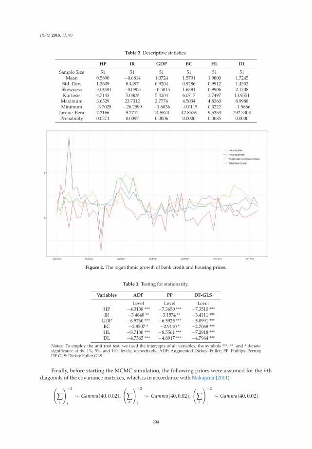
JRFM 2018, 11, 90
Table 2. Descriptive statistics.
HP IR GDP BC HL DL
Sample Size 51 51 51 51 51 51Mean 0.5890 −0.6814 1.0724 1.5791 1.9800 1.7245
Std. Dev. 1.2609 8.4497 0.9204 0.9286 0.9912 1.4552Skewness −0.3381 −0.0905 −0.5015 1.6381 0.9906 2.1208Kurtosis 4.7143 5.0809 5.4204 6.0717 3.7497 13.9351
Maximum 3.6529 23.7312 2.7776 4.5034 4.8360 8.9988Minimum −3.7025 −26.2599 −1.6036 −0.0115 0.3222 −1.9866
Jarque–Bera 7.2166 9.2712 14.5874 42.8576 9.5353 292.3303Probability 0.0271 0.0097 0.0006 0.0000 0.0085 0.0000
Figure 2. The logarithmic growth of bank credit and housing prices.
Table 3. Testing for stationarity.
Variables ADF PP DF-GLS
Level Level LevelHP −4.3138 *** −7.3650 *** −7.3510 ***IR −3.4648 ** −3.1574 ** −3.4111 ***
GDP −6.5760 *** −6.5925 *** −5.0991 ***BC −2.8507 * −2.9110 * −2.7068 ***HL −8.7130 *** −8.5561 *** −7.2918 ***DL −4.7565 *** −4.8917 *** −4.7964 ***
Notes: To employ the unit root test, we used the intercepts of all variables; the symbols ***, **, and * denotesignificance at the 1%, 5%, and 10% levels, respectively. ADF: Augmented Dickey–Fuller; PP: Phillips–Perron;DF-GLS: Dickey Fuller GLS.
Finally, before starting the MCMC simulation, the following priors were assumed for the i-thdiagonals of the covariance matrices, which is in accordance with Nakajima (2011):(
∑ς
)−2
i
∼ Gamma(40, 0.02),
(∑α
)−2
i
∼ Gamma(40, 0.02),
(∑h
)−2
i
∼ Gamma(40, 0.02).
204
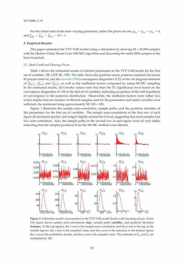
JRFM 2018, 11, 90
For the initial state of the time-varying parameter, rather flat priors are set; μβ0 = μa0 = μh0 = 0,and ∑β0
= ∑a0= ∑h0
= 10 × I.
5. Empirical Results
This paper estimated the TVP-VAR model using a simulation by drawing M = 20,000 sampleswith the Markov Chain Monte Carlo (MCMC) algorithm and discarding the initial 2000 samples in theburn-in period.
5.1. Bank Credit and Housing Prices
Table 4 shows the estimated results of selected parameters in the TVP-VAR model for the firstset of variables: (IR, GDP, BC, HP). The table shows the posterior mean, posterior standard deviation,95 percent interval, and the Geweke (1992) convergence diagnostics (CD) of the i-th diagonal elementsof(∑ς
)i, (∑a)i and (∑h)i, as well as the inefficient factors computed by using MCMC sampling.
In the estimated results, all Geweke values were less than the 5% significance level based on theconvergence diagnostics of 1.96 in the first set of variables, indicating acceptance of the null hypothesisof convergence to the posterior distribution. Meanwhile, the inefficient factors were rather low,which implies that the number of efficient samples used for the parameters and stated variables weresufficient, the minimum being approximately M/100 = 200.
Figure 3 illustrates the sample auto-correlation, sample paths, and the posterior densities ofthe parameters for the first set of variables. The sample auto-correlations in the first row of eachfigure all decreased quickly and ranged slightly around the 0 level, suggesting that most samples hadlow auto-correlation. Also, the sample paths in the second row in each figure were all very stable,indicating that the samples produced from the MCMC method were efficient.
Figure 3. Estimation results of parameters in the TVP-VAR model (bank credit–housing prices). Notes:The figure shows sample auto-correlations (top), sample paths (middle), and posterior densities(bottom). In the top figures, the x-axis is the sample auto-correlation, and the y-axis is the lag; in themiddle figures, the x-axis is the sampled value, and the y-axis is the iteration; in the bottom figure,the x-axis is the probability density, and the y-axis is the sampled value. The estimates of Σζ and Σa aremultiplied by 100.
205
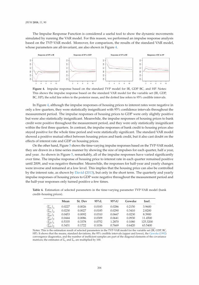
JRFM 2018, 11, 90
The Impulse Response Function is considered a useful tool to show the dynamic movementssimulated by running the VAR model. For this reason, we performed an impulse response analysisbased on the TVP-VAR model. Moreover, for comparison, the results of the standard VAR model,whose parameters are all-invariant, are also shown in Figure 4.
Figure 4. Impulse response based on the standard TVP model for IR, GDP BC, and HP. Notes:This shows the impulse response based on the standard VAR model for the variable set (IR, GDP,BC, HP); the solid line refers to the posterior mean, and the dotted line refers to 95% credible intervals.
In Figure 4, although the impulse responses of housing prices to interest rates were negative inonly a few quarters, they were statistically insignificant with 95% confidence intervals throughout themeasurement period. The impulse responses of housing prices to GDP were only slightly positivebut were also statistically insignificant. Meanwhile, the impulse responses of housing prices to bankcredit were positive throughout the measurement period, and they were only statistically insignificantwithin the first three quarters. In contrast, the impulse responses of bank credit to housing prices alsostayed positive for the whole time period and were statistically significant. The standard VAR modelshowed a positive mutual effect between housing prices and bank credit, but it also cast doubt on theeffects of interest rate and GDP on housing prices.
On the other hand, Figure 5 shows the time-varying impulse responses based on the TVP-VAR model,they are drawn in a time-series manner by showing the size of impulses for each quarter, half a year,and year. As shown in Figure 5, remarkably, all of the impulse responses have varied significantlyover time. The impulse response of housing price to interest rate in each quarter remained positiveuntil 2009, and was negative thereafter. Meanwhile, the responses for half-year and yearly changeswere inverse and remained at a low level. This implies that the housing price can also be controlledby the interest rate, as shown by David (2013), but only in the short term. The quarterly and yearlyimpulse responses of housing prices to GDP were negative throughout the measurement period andthe half-year responses only turned positive a few times.
Table 4. Estimation of selected parameters in the time-varying parameter TVP-VAR model (bankcredit–housing prices).
Mean St. Dev 95%L 95%U Geweke Inef.(∑ς
)1 0.0227 0.0026 0.0183 0.0286 0.2150 3.9600(
∑ς
)2 0.0230 0.0027 0.0185 0.0290 0.3410 2.8200
(∑a)1 0.0453 0.0092 0.0310 0.0667 0.0230 8.3900(∑a)2 0.0444 0.0086 0.0309 0.0641 0.0930 11.4500(∑h)1 0.5335 0.3378 0.0752 1.2870 0.1080 125.3200(∑h)2 0.3431 0.1722 0.1036 0.7669 0.6420 63.5400
Notes: This is the estimation result of selected parameters in the TVP-VAR model for the variable set (IR, GDP, BC,HP). It shows that the means, standard deviations, the 95% credible intervals (upper and lower), the Geweke (1992)convergence diagnostics, and the number of inefficient samples are part of the diagonal elements of the covariancematrices; the estimates of Σς and Σa are multiplied by 100.
206

JRFM 2018, 11, 90
Figure 5. Impulse response for three different horizons. Notes: This shows the impulse response of theTVP-VAR model for the variable set of (IR, GDP, BC, HP); HP represents housing prices, BC representsbank credit, and IR represents the interest rate; the solid line refers to the time-varying impulseresponses for each quarter; the dashed line refers to half-year responses; and the dotted line refers toyearly responses.
We can see that both the impulse responses of the housing price to bank credit and the reverse werepositive throughout the sample period, which proves that although the mutual effect between housingprice and bank credit may vary between the different sides, in the market as a whole, the mutual effectwas still positive throughout the sample period in China.
In addition, we can also notice that the effect of the housing price on bank credit was strongerthan the influence of bank credit on the housing price. This also implies that the banking and creditsystem will be greatly affected if the housing price begins to fluctuate wildly.
5.2. Housing Loans and Housing Prices
Table 5 shows the estimated results of the selected parameters in the TVP-VAR model for thesecond set of variables: (IR, GDP, HL, HP). In the estimated results, all Geweke values were less thanthe 5% significance level based on the convergence diagnostics of 1.96 in the first set of variables,indicating acceptance of the null hypothesis of convergence to the posterior distribution. Meanwhile,the number of inefficient factors was rather low, which implies that the number of efficient samples forthe parameters and stated variables was sufficient, the minimum being approximately M/100 = 200.
Figure 6 illustrates the sample auto-correlation, sample paths, and posterior densities of theparameters for the second set of variables. The sample auto-correlation shown in the first row ofeach figure decreased quickly and ranged around the 0 level, suggesting that most samples had lowauto-correlation. Also, the sample paths shown in the second row of each figure were all very stable,indicating that the samples produced from the MCMC method were efficient.
Figure 7 shows the impulse response functions based on the standard VAR model for the secondvariable set (IR, GDP, HL, HP). In Figure 7, the impulse responses of housing prices to the interest rate
207
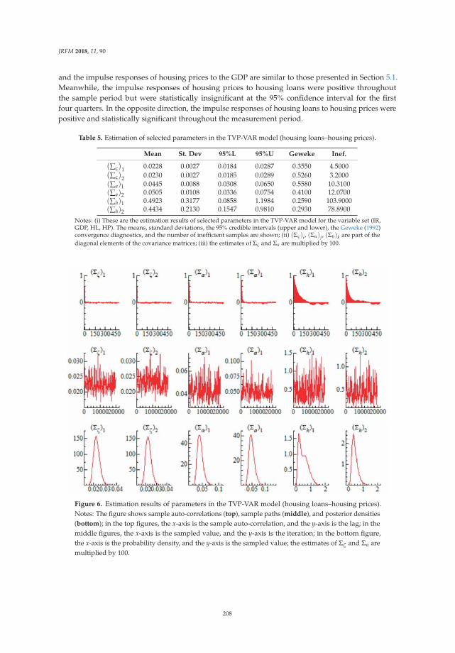
JRFM 2018, 11, 90
and the impulse responses of housing prices to the GDP are similar to those presented in Section 5.1.Meanwhile, the impulse responses of housing prices to housing loans were positive throughoutthe sample period but were statistically insignificant at the 95% confidence interval for the firstfour quarters. In the opposite direction, the impulse responses of housing loans to housing prices werepositive and statistically significant throughout the measurement period.
Table 5. Estimation of selected parameters in the TVP-VAR model (housing loans–housing prices).
Mean St. Dev 95%L 95%U Geweke Inef.(∑ς
)1 0.0228 0.0027 0.0184 0.0287 0.3550 4.5000(
∑ς
)2 0.0230 0.0027 0.0185 0.0289 0.5260 3.2000
(∑a)1 0.0445 0.0088 0.0308 0.0650 0.5580 10.3100(∑a)2 0.0505 0.0108 0.0336 0.0754 0.4100 12.0700(∑h)1 0.4923 0.3177 0.0858 1.1984 0.2590 103.9000(∑h)2 0.4434 0.2130 0.1547 0.9810 0.2930 78.8900
Notes: (i) These are the estimation results of selected parameters in the TVP-VAR model for the variable set (IR,GDP, HL, HP). The means, standard deviations, the 95% credible intervals (upper and lower), the Geweke (1992)convergence diagnostics, and the number of inefficient samples are shown; (ii) (Σς)i , (Σα)j, (Σh)k are part of thediagonal elements of the covariance matrices; (iii) the estimates of Σς and Σa are multiplied by 100.
Figure 6. Estimation results of parameters in the TVP-VAR model (housing loans–housing prices).Notes: The figure shows sample auto-correlations (top), sample paths (middle), and posterior densities(bottom); in the top figures, the x-axis is the sample auto-correlation, and the y-axis is the lag; in themiddle figures, the x-axis is the sampled value, and the y-axis is the iteration; in the bottom figure,the x-axis is the probability density, and the y-axis is the sampled value; the estimates of Σζ and Σa aremultiplied by 100.
208
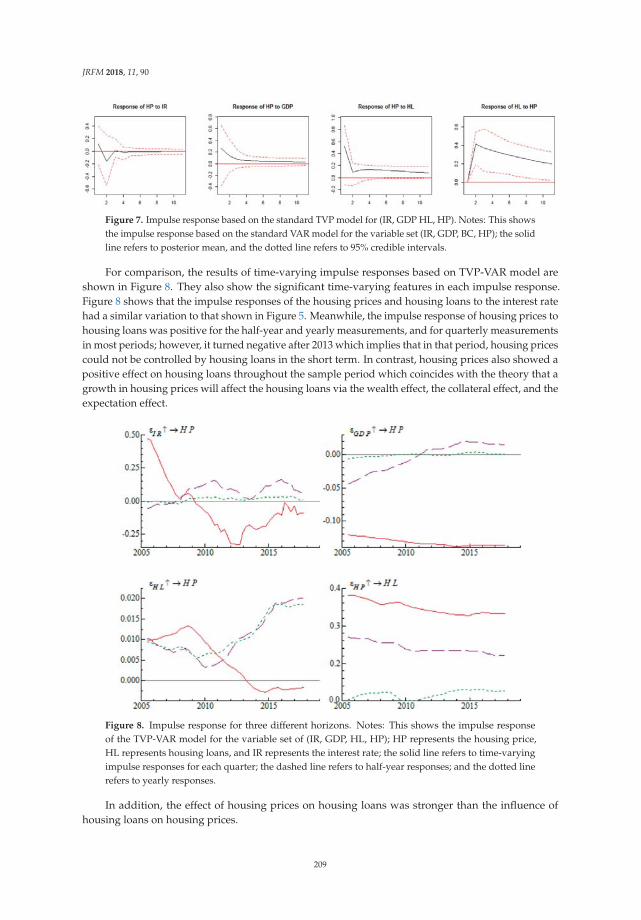
JRFM 2018, 11, 90
Figure 7. Impulse response based on the standard TVP model for (IR, GDP HL, HP). Notes: This showsthe impulse response based on the standard VAR model for the variable set (IR, GDP, BC, HP); the solidline refers to posterior mean, and the dotted line refers to 95% credible intervals.
For comparison, the results of time-varying impulse responses based on TVP-VAR model areshown in Figure 8. They also show the significant time-varying features in each impulse response.Figure 8 shows that the impulse responses of the housing prices and housing loans to the interest ratehad a similar variation to that shown in Figure 5. Meanwhile, the impulse response of housing prices tohousing loans was positive for the half-year and yearly measurements, and for quarterly measurementsin most periods; however, it turned negative after 2013 which implies that in that period, housing pricescould not be controlled by housing loans in the short term. In contrast, housing prices also showed apositive effect on housing loans throughout the sample period which coincides with the theory that agrowth in housing prices will affect the housing loans via the wealth effect, the collateral effect, and theexpectation effect.
Figure 8. Impulse response for three different horizons. Notes: This shows the impulse responseof the TVP-VAR model for the variable set of (IR, GDP, HL, HP); HP represents the housing price,HL represents housing loans, and IR represents the interest rate; the solid line refers to time-varyingimpulse responses for each quarter; the dashed line refers to half-year responses; and the dotted linerefers to yearly responses.
In addition, the effect of housing prices on housing loans was stronger than the influence ofhousing loans on housing prices.
209
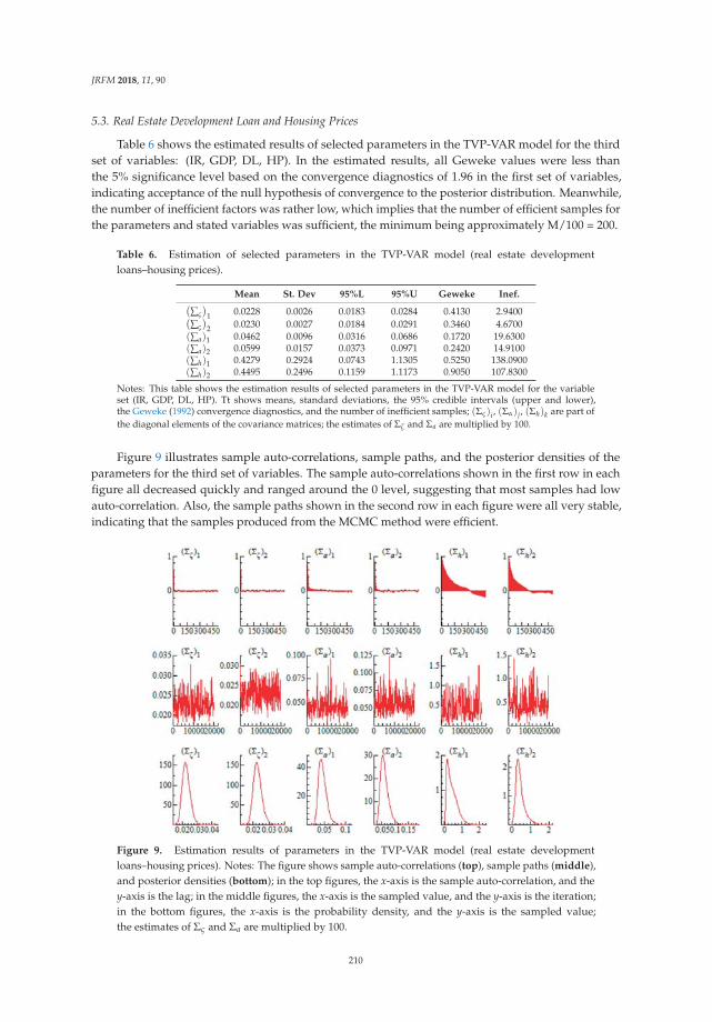
JRFM 2018, 11, 90
5.3. Real Estate Development Loan and Housing Prices
Table 6 shows the estimated results of selected parameters in the TVP-VAR model for the thirdset of variables: (IR, GDP, DL, HP). In the estimated results, all Geweke values were less thanthe 5% significance level based on the convergence diagnostics of 1.96 in the first set of variables,indicating acceptance of the null hypothesis of convergence to the posterior distribution. Meanwhile,the number of inefficient factors was rather low, which implies that the number of efficient samples forthe parameters and stated variables was sufficient, the minimum being approximately M/100 = 200.
Table 6. Estimation of selected parameters in the TVP-VAR model (real estate developmentloans–housing prices).
Mean St. Dev 95%L 95%U Geweke Inef.(∑ς
)1 0.0228 0.0026 0.0183 0.0284 0.4130 2.9400(
∑ς
)2 0.0230 0.0027 0.0184 0.0291 0.3460 4.6700
(∑a)1 0.0462 0.0096 0.0316 0.0686 0.1720 19.6300(∑a)2 0.0599 0.0157 0.0373 0.0971 0.2420 14.9100(∑h)1 0.4279 0.2924 0.0743 1.1305 0.5250 138.0900(∑h)2 0.4495 0.2496 0.1159 1.1173 0.9050 107.8300
Notes: This table shows the estimation results of selected parameters in the TVP-VAR model for the variableset (IR, GDP, DL, HP). Tt shows means, standard deviations, the 95% credible intervals (upper and lower),the Geweke (1992) convergence diagnostics, and the number of inefficient samples; (Σς)i , (Σα)j, (Σh)k are part ofthe diagonal elements of the covariance matrices; the estimates of Σζ and Σa are multiplied by 100.
Figure 9 illustrates sample auto-correlations, sample paths, and the posterior densities of theparameters for the third set of variables. The sample auto-correlations shown in the first row in eachfigure all decreased quickly and ranged around the 0 level, suggesting that most samples had lowauto-correlation. Also, the sample paths shown in the second row in each figure were all very stable,indicating that the samples produced from the MCMC method were efficient.
Figure 9. Estimation results of parameters in the TVP-VAR model (real estate developmentloans–housing prices). Notes: The figure shows sample auto-correlations (top), sample paths (middle),and posterior densities (bottom); in the top figures, the x-axis is the sample auto-correlation, and they-axis is the lag; in the middle figures, the x-axis is the sampled value, and the y-axis is the iteration;in the bottom figures, the x-axis is the probability density, and the y-axis is the sampled value;the estimates of Σς and Σa are multiplied by 100.
210
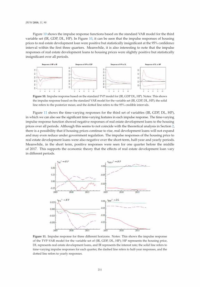
JRFM 2018, 11, 90
Figure 10 shows the impulse response functions based on the standard VAR model for the thirdvariable set (IR, GDP, DL, HP). In Figure 10, it can be seen that the impulse responses of housingprices to real estate development loan were positive but statistically insignificant at the 95% confidenceinterval within the first three quarters. Meanwhile, it is also interesting to note that the impulseresponses of real estate development loans to housing prices were slightly positive but statisticallyinsignificant over all periods.
Figure 10. Impulse response based on the standard TVP model for (IR, GDP DL, HP). Notes: This showsthe impulse response based on the standard VAR model for the variable set (IR, GDP, DL, HP); the solidline refers to the posterior mean; and the dotted line refers to the 95% credible intervals.
Figure 11 shows the time-varying responses for the third set of variables (IR, GDP, DL, HP),in which we can also see the significant time-varying features in each impulse response. The time-varyingimpulse response function showed negative responses of real estate development loans to the housingprices over all periods. Although this seems to not coincide with the theoretical analysis in Section 2,there is a possibility that if housing prices continue to rise, real development loans will not expandand may even reduce under government regulation. The impulse responses of the housing price toreal estate development loans were also negative over the short-term, half-year and yearly periods.Meanwhile, in the short term, positive responses were seen for one quarter before the middleof 2017. This supports the economic theory that the effects of real estate development loan varyin different periods.
Figure 11. Impulse response for three different horizons. Notes: This shows the impulse responseof the TVP-VAR model for the variable set of (IR, GDP, DL, HP); HP represents the housing price,DL represents real estate development loans, and IR represents the interest rate; the solid line refers totime-varying impulse responses for each quarter, the dashed line refers to half-year responses, and thedotted line refers to yearly responses.
211

JRFM 2018, 11, 90
In addition, we can see that the effect of housing prices on real estate development loans was alsostronger than the effect in the opposite direction.
6. Conclusions
The limitation of the VAR model is that it cannot capture possible non-linearity or time variation inthe lag structure of the model, and it also cannot capture possible heteroscedasticity of the shocks andnon-linearity in the simultaneous relations among the variables of the model. Meanwhile, the TVP-VARmodel with stochastic volatility is so flexible and robust that it can capture possible changes in theunderlying structure of the economy. For this reason, in accordance with following Nakajima (2011),we used the TVP-VAR model with stochastic volatility to study the dynamic relationship betweenbank credit and housing prices in China from 2005Q2 to 2007Q4. Moreover, in order to study howbank credit affects buyers and developers, we also performed the same estimation for housing loansand real estate development loans. Finally, we obtained the following findings.
Firstly, the relationships between housing prices, bank credit, housing loans, and realestate development loans showed significant time-varying features, meaning that they change indifferent periods.
Secondly, the mutual effect between housing prices and bank credit varied between the different sides.In the market as a whole, the mutual effect over the whole sample period in China was shown tobe positive. On the demand side, the mutual effect between housing prices and housing loans wasalso positive in most measured periods. However, we still saw that the effect of housing loans onhousing prices for each quarter was negative in some years which casts doubt on the controllabilityof the housing loans control channel which is intended to control housing prices in the short term.On the demand side, the effect of housing prices was shown to be negative which seems to notcoincide with the theoretical analysis in Section 2, but there is a possibility that is influenced bygovernment regulation. In the opposite direction, the effect of real estate development loans onhousing prices was shown to be negative in the long term, half-year and yearly periods, but positivefor the short-term, quarterly, and some yearly periods, which coincides with the theoretical analysis.
Finally, it is also interesting to note that influences of housing prices on all kinds of bank creditare stronger than those in the opposite direction. This implies that the People’s Bank of China shouldpay attention to the risk that a housing price collapse would have effects on the bank credit system.
Based on the TVP-VAR with stochastic volatility, we identified the time-varying effects of bankcredit on housing prices and the reverse in the Chinese housing market. Furthermore, we founddifferent time-varying relationships between these two factors on the demand side and the supply side.Nevertheless, we did not find evidence of, or observe, any reasons why a time-varying effect happenedduring this period. This could be a future study direction.
Author Contributions: S.H. conceived and designed the experiments; X.H. performed the experiments,analyzed the data, and contributed reagents/materials/analysis tools; X.H., X.-J.C., and S.H. drafted the manuscript.
Funding: This research was supported by JSPS KAKENHI Grant Number 17K18564 and (A) 17H00983.
Acknowledgments: We are grateful to the three anonymous referees for their helpful comments and suggestions.
Conflicts of Interest: The authors declare no conflicts of interest. The founding sponsors had no role in the designof the study, in the collection, analyses, or interpretation of data, in the writing of the manuscript, or in the decisionto publish the results.
References
Black, Fischer. 1976. Studies of Stock Market Volatility Changes. In Proceedings of the 1976 Meetings of the Businessand Economic Statistics Section. Washington DC: American Statistical Association, pp. 177–81.
Cai, Weina, and Sen Wang. 2018. The Time-Varying Effects of Monetary Policy on Housing Prices in China: AnApplication of TVP-VAR Model with Stochastic Volatility. International Journal of Business Management 13:149–57. [CrossRef]
212

JRFM 2018, 11, 90
Collyns, Charles, and Abdelhak Senhadji. 2002. Lending Booms, Real Estate, and The Asian Crisis. IMF WorkingPaper. Washington DC: IMF, pp. 1–46. Available online: https://ssrn.com/abstract=879360 (accessed on 10September 2018).
Davis, E. Philip, and Haibin Zhu. 2011. Bank lending and commercial property cycles: Some cross-countryevidence. Journal of International Money and Finance 30: 1–21. [CrossRef]
David, Nissim Ben. 2013. Predicting housing prices according to expected future interest rate. Applied Economics45: 3044–48. [CrossRef]
Geweke, John. 1992. Evaluating the Accuracy of Sampling-Based Approaches to the Calculation of PosteriorMoments. In Bayesian Statistics 4. Edited by José-Miguel Bernardo, James O. Berger, Alexander Philip Dawidand Adrian Frederick Melhuish Smith. Oxford: Oxford University Press, pp. 169–93.
Gerlach, Stefan, and Wensheng Peng. 2005. Bank Lending and Property Prices in Hong Kong. Journal of Banking &Finance 29: 461–81. [CrossRef]
Goodhart, Charles, and Boris Hofmann. 2008. House Prices, Money, Credit and the Macroeconomy. Oxford Reviewof Economic Policy 24: 180–205. Available online: https://EconPapers.repec.org/RePEc:oup:oxford:v:24:y:2008:i:1:p:180-205 (accessed on 20 October 2018). [CrossRef]
Gimeno, Ricardo, and Carmen Martínez Carrascal. 2010. The relationship between house prices and housepurchase loans: The Spanish case. Journal of Banking & Finance 34: 1849–55. [CrossRef]
Hong, Liming. 2014. The Dynamic Relationship between Real Estate Investment and Economic Growth: Evidencefrom Prefecture City Panel Data in China. IERI Procedia 7: 2–7. [CrossRef]
McQuinn, Kieran, and Gerard O’Reilly. 2008. Assessing the role of income and interest rates in determining houseprices. Economic Modelling 25: 377–90. [CrossRef]
Mwabutwa, Chance, Nicola Viegi, and Manoel Bittencourt. 2016. Evolution of Monetary Policy TransmissionMechanism in Malawi: A TVP-VAR Approach. Journal of Economic Development 41: 33–55.
Mora, Nada. 2008. The Effect of Bank Credit on Asset Prices: Evidence from the Japanese Real Estate Boom duringthe 1980s. Journal of Money, Credit and Banking 40: 57–87. Available online: https://www.jstor.org/stable/25096240 (accessed on 19 September 2018). [CrossRef]
Nakajima, Jouchi. 2011. Time-Varying Parameter VAR Model with Stochastic Volatility: An Overview of Methodology andEmpirical Applications. IMES Discussion Paper Series, 11-E-09; Tokyo: Institute for Monetary and EconomicStudies, Bank of Japan.
Primiceri, Giorgio. 2005. Time Varying Structural Vector Autoregressions and Monetary Policy. The Review ofEconomic Studies 72: 821–52. [CrossRef]
Qin, Lin, and Yimin Yao. 2012. A Study of the Relationship between Bank Credit and Real Estate Prices.Comparative Economic & Social Systems 2: 188–202. (In Chinese)
Shephard, Neil. 1996. Statistical Aspects of ARCH and Stochastic Volatility. In Time Series Models in Econometrics,Finance and Other Fields. London: Chapman & Hall, pp. 1–67.
Taylor, Stephen J. 1986. Modelling Financial Time Series. Chichester: John Wiley.Tian, Shuairu, and Shigeyuki Hamori. 2016. Time-Varying Price Shock Transmission and Volatility Spillover in
Foreign Exchange, Bond, Equity, and Commodity Markets: Evidence from the United States. North AmericanJournal of Economics and Finance 38: 163–71. [CrossRef]
Yuan, Nannan, and Shigeyuki Hamori. 2014. Crowding-out effects of affordable and unaffordable housing inChina, 1999–2010. Applied Economics 46: 4318–33. [CrossRef]
Yang, Lu, and Shigeyuki Hamori. 2018. Modeling the dynamics of international agricultural commodity prices:A comparison of GARCH and stochastic volatility models. Annals of Financial Economics 13: 1–20. [CrossRef]
© 2018 by the authors. Licensee MDPI, Basel, Switzerland. This article is an open accessarticle distributed under the terms and conditions of the Creative Commons Attribution(CC BY) license (http://creativecommons.org/licenses/by/4.0/).
213

Journal of
Risk and FinancialManagement
Article
Is Window-Dressing around Going Public Beneficial?Evidence from Poland
Joanna Lizinska * and Leszek Czapiewski
Department of Corporate Finance, Poznan University of Economics and Business, al. Niepodległosci 10,61-875 Poznan, Poland; [email protected]* Correspondence: [email protected]; Tel.: +48-61-854-3862
Received: 13 December 2018; Accepted: 18 January 2019; Published: 21 January 2019
Abstract: The informativeness of financial reports has been of a great importance to both investorsand academics. Earnings are crucial for evaluating future prospects and determining company value,especially around milestone events such as initial public offerings (IPO). If investors are misled bymanipulated earnings, they could pay too high a price and suffer losses in the long-term when pricesadjust to real value. We provide new evidence on the relationship between earnings management andthe long-term performance of IPOs as we test the issue with a methodology that has not been appliedso far for issues in Poland. We use a set of proxies of earnings management and test the long-termIPO performance under several factor models (CAPM, and three extensions of the Fama-Frenchmodel). Aggressive IPOs perform very poorly later and earn severe negative stock returns up tothree years after going public. The difference in returns in accrual quantiles is statistically significantin almost half of methodology settings. The results seem to suggest that investors might not beable to discount pre-IPO abnormal accruals and could be overoptimistic. Once the true earningsperformance is revealed over time, the market makes downward price corrections.
Keywords: earnings management; earnings manipulation; earnings quality; initial public offering;IPO; asset pricing model
1. Introduction
Financial statements are a very important source of information for stakeholders. Businesses areexpected to follow numerous accounting standards and rules in the process of recording activities andtransactions properly. Managers are given discretion to some extent in reporting a company’ situation.Managerial discretion in reporting has both benefits and disadvantages. Managers should use theirunique knowledge to make financial statements more informative. However, managers may also usetheir judgment in reporting to mislead other stakeholders. Following a high information asymmetrybetween issuers and investors of initial public offering (IPO) companies at the time of the going public,investors rely heavily on financial statements. Simultaneously, IPO firms have an opportunity tomanage earnings as usually little is known about market newcomers. They also have incentives to doso as the moment of going public is a very important event that attracts a lot of attention.
The key objective of this research is to assess whether the long-term performance of initial publicofferings in Poland differs systematically according to the magnitude of around-the-issue earningsmanagement. Previously published studies on Polish IPOs reported results using the event-timeapproach, according to the buy-and-hold abnormal returns (BHAR) or cumulative abnormal returns(CAR). They have been both very popular measures of the long-term performance. Fama (1998)and other researchers (Barber and Lyon 1997; Lyon et al. 1999; Jegadeesh and Karceski 2009) pointout the deficiencies of the event-time approach such as skewness bias, violations in cross-sectionalindependence, or re-balancing bias. Our study is the first one that discusses the relationship between
JRFM 2019, 12, 18; doi:10.3390/jrfm12010018 www.mdpi.com/journal/jrfm214
JRFM 2019, 12, 18
earnings management and the long-term IPO performance in Poland with the alternative methodology,namely the calendar-time portfolio approach. The method that we apply is mentioned by manyresearchers as mitigating many statistical problems arising in long-term event studies. Given thegeneral lack of evidence on explanations of long-term abnormal returns with the calendar-timeportfolio based on the opportunistic earnings management behavior for the Polish capital market,this is the area where this study contributes to the existing literature as it provides internationalinsights into the discussion. Poland is an important area of economic growth in Europe which inclinesacademics to address many financial issues and makes possible conclusions important. The resultsof the long-term implications of earnings management for IPOs in Poland are not obvious. First, it isbecause of the theoretical background that is briefly summarized in the paper. Second, Poland hasdifferent characteristics to other markets. This country has undertaken a long journey of economicliberalization since the transition of its economy. During the period we examine, it has been classifiedas an emerging market by all of the leading agencies. Just recently, though, it has been ranked by FTSERussell as a developed market. The uniqueness of studies on an emerging market that transforms intoa developed economy, is a strong and motivating argument for taking empirical research. This is theonly way to uncover mechanisms of capital markets based on the fact that direct comparison withUS-centered research is limited. Although Poland is the eighth largest economy in the European Union(EU) and the largest among Central and Eastern European countries in the EU, Polish companies’capitalization is much smaller in comparison to US stock markets. It has deep consequences for amethodology of empirical research as many methodological solutions have been proposed for theUS, which is an incomparably larger market. Applying these solutions to much smaller marketsencounters numerous practical problems. This paper is one of the pieces of the research stream thattouches the uniqueness of less-developed economies and faces the difficulty of methodological issuesfor small capital markets. All of these arguments taken together make the research on the long-termimplications of earnings management for Polish IPOs challenging and contributing to the existingliterature. Under the overoptimism hypothesis, we expect that the greater the earnings managementlevel around the time of the issue, the larger the long-term price correction.
Both earnings management and abnormal long-term market performance of IPOs cannot bemeasured directly so they are observed with proxies. We proxy for earnings management usingdiscretionary accruals. Factor regressions produce intercepts for rolling IPO portfolios that proxyfor abnormal long-term performance. As alternative methodologies suffer from different types ofbiases as well as have their strong points, we provide a broad set of robustness checks. Accrualsare estimated as the difference between real accruals and non-discretionary accruals where thelatter are estimated using the cross-sectional industry-year regressions under the Jones model(Jones 1991), the modified Jones model (Dechow et al. 1995), the McNichols model (McNichols 2000),and Ball–Shivakumar model (Ball and Shivakumar 2006). We also apply a broad set of assetpricing models to assess the long-term performance. Empirically, we start with the CapitalAsset Pricing Model (Sharpe 1964; Lintner 1969), and extend the analysis of long-term abnormalperformance with estimating monthly risk premiums under three multifactor models: the Fama-Frenchthree-factor model (Fama and French 1993), the Carhart four-factor model (Carhart 1997), and the latestinnovation—namely, the Fama-French five-factor model (Fama and French 2015, 2016).
Our results show strong long-term underperformance of initial public offerings in Poland usingthe calendar-time portfolio approach. Alphas are statistically and economically significant for bothlow- and high-accrual IPO firms. Both, conservative and aggressive IPO companies experience arelative decline in market value in the long run. The magnitude of IPO negative returns is sensitiveto the methodology, but it does not change the conclusions about long-term IPO underperformance.Annualized abnormal returns range from −8.2% to −13.7% for conservative IPO companies, whereasthe span for aggressive IPO companies is from −12.1% up to even −20.5%. Importantly, we reportthat more conservative IPO firms outperform firms that managed their earnings more aggressively.The average difference between quantiles totals 5.9 percentage points annually, and it ranges from 2.0
215

JRFM 2019, 12, 18
percentage points annually up to even 10.4 percentage points per year. Average annualized alphas forconservative IPO firms equals −10.2%, whereas it is −16.1% for aggressive IPO firms. The averageabnormal returns are much more negative for the aggressive IPO companies and this difference isstatistically significant in almost half of methodology settings. The rest of the paper is organized asfollows. Section 2 gives a brief discussion of the existing literature. Section 3 briefly describes the datasources, details earnings management proxies and methods of the long-run performance measures.Section 4 contains descriptive statistics and a short risk premium presentation. Section 5 presentsevidence on the explanatory power of earnings management for the long-term abnormal performanceand offers tests for robustness of results. Section 6 discusses the empirical results in the light of theexisting comparable evidence on other markets and outlines future research. The last section concludesthe paper.
2. Brief Theoretical Background
The question of earnings management has not been constrained solely to equity issues.Proxies of earnings management have been applied to a broad set of issues in finance whichargues for the importance of earnings management for many company activities (Healy 1985;Liberty and Zimmerman 1986; McNichols and Wilson 1988; Jones 1991; Pourciau 1993; DeFond andJiambalvo 1994; Gaver et al. 1995; Holthausen et al. 1995; Perry and Williams 1994; Teoh et al. 1998b).
The choice whether to manage or not to manage earnings when a firm is planning to sell itsshares to the market for the first time is not obvious. The issue of earnings management relates totwo opposite hypotheses. The first one is connected with the opportunism of IPO issuers. The secondtheory relates to the expected enhanced reporting quality of public companies together with regulatorylimits on discretion, penalties for misreporting, or greater external monitoring.
Analyzing the importance of earnings to investors, Sloan (1996) suggests that the cash flowcomponent may be underweighted and the accrual component may be overweighted. If an IPO firmengages in increasing earnings around going public and investors are not able to recognize the trueinformation content of earnings as indicators of future prospects, they will raise stock prices at issue.In the long-term, when the real performance is revealed and information asymmetries between theissuer and its investors are lower, the market is expected to adjust the IPO prices down. This is one ofthe possible explanations for the long-term underperformance observed for the US IPOs, as well asother developed markets or emerging markets.
Reported earnings consist of cash flows and accruals. Accruals are defined as accountingadjustments to cash flows. If earnings are artificially boosted around going public, it is much easierto proceed with the accrual part than with real cash changes, which justifies accruals as a measureof earnings manipulation. According to different ideas behind the income statement and cash flowstatement, earnings usually differ from cash flows. Following this, accruals appear as a naturalconsequence of this. However, not all the accruals have the same degree of managerial discretion.This inclines us toward decomposing accruals, as in Jones (1991). Some accruals are normal to companyactivities or are exposed to limited managerial discretion. They are non-discretionary components(normal or expected accruals). The discretionary part of accruals (abnormal accruals) proxies forthe earnings manipulation level as these accruals are considered to have been the ‘managed’ part ofthe earnings.
Previous papers suggest that IPO companies manage their earnings for the moment of goingpublic, and usually conclude that companies managing their accruals aggressively also experiencestrong long-term underperformance (Teoh et al. 1998a; DuCharme et al. 2001; Roosenboom et al. 2003;Chen et al. 2005; Pastor-Llorca and Poveda-Fuentes 2011; Ahmad-Zaluki et al. 2011; Xie 2001;Chan et al. 2001). However, Beneish (1998) questions systematic investor valuation errors based oninflated earnings. Along the same lines, Ball and Shivakumar (2005), Ball and Shivakumar (2006) andBall and Shivakumar (2008) argue in favor of more conservative reporting by public companies.
216
JRFM 2019, 12, 18
The research on the links between earnings management and subsequent IPO performance inPoland is scant. Lizinska and Czapiewski (2018a) used the buy-and-hold approach and reported thatmore aggressive IPOs performed poorly in the long run. However, the difference in the long-termabnormal returns between firms with lower and higher discretionary accruals was not robust in allsettings of methodology. Lizinska and Czapiewski (2018b) combined earnings quality around goingpublic with the long-term price behavior and tested the puzzle with OLS regressions based on theBHAR approach. Robustness tests allowed for a conclusion that the long-term buy-and-hold abnormalreturns of initial public offerings completed before the peak of the crisis were negatively related toearnings management around IPO date.
3. Sources of Data and Methodology
The research sample covers initial public offerings listed on the Warsaw Stock Exchange (WSE)from January 2002 to December 2014. We include only offerings from the main equity market, and thosewithout prior quotation on alternative markets. The sample covers only issues with a new commonstock issuance. Delisted companies are included both in the IPO sample and in the benchmark sample.Initial public offerings are restricted to the non-financial industry.
The data are derived from Notoria Serwis, the official site of the WSE and InfoStrefa.com. Marketreturns for companies are based on adjusted close prices and they include dividends, splits andpre-emptive rights. The list of IPOs ends in 2014 but the market data cover a longer period as it wasnecessary to calculate long-term adjusted returns.
The aim of the research relates to the extent to which earnings management is related to thesubsequent long-term abnormal market performance of IPO firms in Poland. As none of thiscan be observed directly, we rely on proxies. Both, the estimates of earnings management andlong-term performance have been much debated in the literature. We do not aim to expand themethodology in this research, but apply a broad set of methodology settings derived from the existingliterature. The empirical modelling encompasses five time-consuming steps: earnings managementproxy estimation, ranking of IPOs according to aggressive or conservative earnings management,risk premiums estimation for a set of asset pricing models, estimation of the measure of long-termrisk-adjusted IPO performance according to the calendar-time portfolio approach in accrual quantiles,and estimation of an equivalent regression of the difference in intercepts between the aggressive andconservative IPOs.
In this research, the level of earnings manipulation is estimated with accrual-based methods. It ismuch easier to manage profits with the accrual part of earnings than with real cash changes. It isa strong argument to use accruals as a measure of earnings manipulation. We run cross-sectionalregressions for every industry and every year to assess the non-discretionary part of accruals (NDACC).In the next step, we relate them to real accruals to get the discretionary part (DACC), which isan earnings manipulation estimator. Real accruals reflect the accounting meaning of adjustmentsand are composed of non-cash current assets change, change in current liabilities, and depreciation.A prerequisite for running industry-year regression is a minimum industry size of five companies.An embargo of two years is imposed on an IPO firm which excludes each IPO from the benchmarkgroup for other IPO companies during this period. Cross-sectional regressions allow us to incorporatechanges in economic conditions that affect a particular industry. Accruals, as well as their components,are scaled with lagged assets (A) to reduce heteroscedasticity in residuals for accruals and theircomponents (Ronen and Yaari 2008).
We use set of accrual-based earnings management proxies. First, we use the Jones model(Jones 1991) which assumes that the level of expected accruals is largely determined by gross property,plant, and equipment (PPE) and change in revenues (ΔREV) as in the following equation
NDACCJit = αi1
(1
Ai,t
)+ αi2ΔREVi,t + αi3PPEi,t + εi,t. (1)
217
JRFM 2019, 12, 18
Dechow et al. (1995) extended the Jones model and proposed a modified version. They includedthe change in trade receivables (ΔREC) to account for the possibility of credit sales manipulation byinducing sales in certain periods without real money inflows. Thus, increases in trade receivables areexcluded from the change in revenues as in the equation
NDACCmJit = αi1
(1
Ai,t
)+ αi2(ΔREVi,t − ΔRECi,t) + αi3PPEi,t + εi,t. (2)
We also consider other improvements to the Jones model. The Dechow and Dichev (2002) model,in the version proposed by McNichols (2000), considers extensions of the Jones model by current, past,and future cash flow from operating activities (CFO)
NDACCMcNit = αi1
(1
Ai,t
)+ αi2CFOi,t−1 + αi3CFOi,t+
+αi4CFOi,t+1 + αi5ΔREVi,t + αi6PPEi,t + εi,t(3)
Ball and Shivakumar (2006) incorporate timely loss recognition in the accruals estimation process.They include DCFO which is 1 if the change in cash flows is less than zero, and 0 otherwise, and abook value of fixed assets (FASSET)
NDACCBSit = αi1
(1
Ai,t
)+ αi5ΔREVi,t + FASSETi,t + αi3CFOi,t + αi3DCFOi,t
+αi3CFOi,t · αi3DCFOi,t + εi,t(4)
In the next research step, we rank initial public offerings by discretionary accruals into twoquantiles: conservative for the smallest abnormal accruals (C) and aggressive for largest discretionaryaccruals (A) as in Ahmad-Zaluki et al. (2011). The ranks are given independently for each of theearnings management proxies. Next, portfolios of aggressive or conservative IPO are constructed onthe basis of IPOs that went public within the past 36 months, with monthly rebalancing.
In the main research step, we estimate the long-term abnormal performance across accrualquantiles. Long-term risk-adjusted performance of IPOs is estimated according to a calendar-timeportfolio approach. Given the concerns about proper measure, we use a variety of methodologicalsettings. Thus, we deliver a broad set of robustness checks. We use the explanation for the cross-sectionof average returns steaming from the capital asset pricing model (Sharpe 1964; Lintner 1969),Fama and French (1993) three-factor model, the Carhart (1997) four-factor model, and the Fama andFrench (2015) five-factor model (CAPM, 3FF, 4C, and 5FF, hereafter).
The first model used in the study is the CAPM. Jensen’s alpha is given by the relationship betweenexcess return and beta
RPt − RF
t = α + β(
RMt − RF
t
)+ εP
t , (5)
where RPt is the calendar time portfolio return, RF
t is the risk-free rate calculated with WIBOR, RMt is
the monthly market return based on the stock market index (Warsaw Stock Index, WIG), and εPt is the
error term.Next, the estimate of alpha is derived from the Fama and French (1993) three-factor model
RPt − RF
t = α + βM
(RM
t − RFt
)+ βSMBSMBt + βHML HMLt + εP
t , (6)
where SMBt is the difference in returns between portfolios of small and big companies, and HMLt isthe average return on the two value portfolios minus the average return on the two growth portfolios.
As an additional check, an intercept is estimated according to the Carhart (1997) four-factor modelas in
RPt − RF
t = α + βRM
(RM
t − RFt
)+ βSMBSMBt + βHMLHMLt + βWMLWMLt, (7)
218
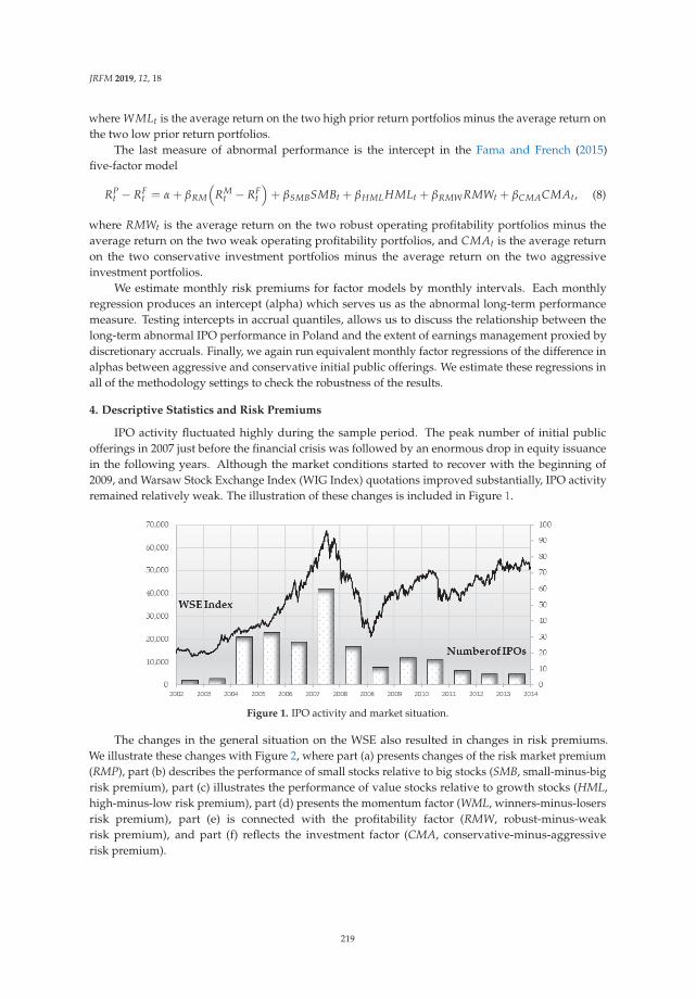
JRFM 2019, 12, 18
where WMLt is the average return on the two high prior return portfolios minus the average return onthe two low prior return portfolios.
The last measure of abnormal performance is the intercept in the Fama and French (2015)five-factor model
RPt − RF
t = α + βRM
(RM
t − RFt
)+ βSMBSMBt + βHMLHMLt + βRMW RMWt + βCMACMAt, (8)
where RMWt is the average return on the two robust operating profitability portfolios minus theaverage return on the two weak operating profitability portfolios, and CMAt is the average returnon the two conservative investment portfolios minus the average return on the two aggressiveinvestment portfolios.
We estimate monthly risk premiums for factor models by monthly intervals. Each monthlyregression produces an intercept (alpha) which serves us as the abnormal long-term performancemeasure. Testing intercepts in accrual quantiles, allows us to discuss the relationship between thelong-term abnormal IPO performance in Poland and the extent of earnings management proxied bydiscretionary accruals. Finally, we again run equivalent monthly factor regressions of the difference inalphas between aggressive and conservative initial public offerings. We estimate these regressions inall of the methodology settings to check the robustness of the results.
4. Descriptive Statistics and Risk Premiums
IPO activity fluctuated highly during the sample period. The peak number of initial publicofferings in 2007 just before the financial crisis was followed by an enormous drop in equity issuancein the following years. Although the market conditions started to recover with the beginning of2009, and Warsaw Stock Exchange Index (WIG Index) quotations improved substantially, IPO activityremained relatively weak. The illustration of these changes is included in Figure 1.
Figure 1. IPO activity and market situation.
The changes in the general situation on the WSE also resulted in changes in risk premiums.We illustrate these changes with Figure 2, where part (a) presents changes of the risk market premium(RMP), part (b) describes the performance of small stocks relative to big stocks (SMB, small-minus-bigrisk premium), part (c) illustrates the performance of value stocks relative to growth stocks (HML,high-minus-low risk premium), part (d) presents the momentum factor (WML, winners-minus-losersrisk premium), part (e) is connected with the profitability factor (RMW, robust-minus-weakrisk premium), and part (f) reflects the investment factor (CMA, conservative-minus-aggressiverisk premium).
219
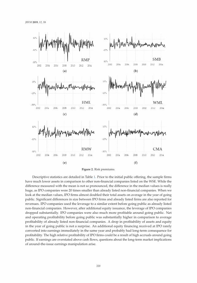
JRFM 2019, 12, 18
(a) (b)
(c) (d)
(e) (f)
Figure 2. Risk premiums.
Descriptive statistics are detailed in Table 1. Prior to the initial public offering, the sample firmshave much lower assets in comparison to other non-financial companies listed on the WSE. While thedifference measured with the mean is not so pronounced, the difference in the median values is reallyhuge, as IPO companies were 20 times smaller than already listed non-financial companies. When welook at the median values, IPO firms almost doubled their total assets on average in the year of goingpublic. Significant differences in size between IPO firms and already listed firms are also reported forrevenues. IPO companies used the leverage to a similar extent before going public as already listednon-financial companies. However, after additional equity issuance, the leverage of IPO companiesdropped substantially. IPO companies were also much more profitable around going public. Netand operating profitability before going public was substantially higher in comparison to averageprofitability of already listed non-financial companies. A drop in profitability of assets and equityin the year of going public is not a surprise. An additional equity financing received at IPO rarelyconverted into earnings immediately in the same year and probably had long-term consequence forprofitability. The high relative profitability of IPO firms could be a result of high accruals around goingpublic. If earnings are overstated above cash flows, questions about the long-term market implicationsof around-the-issue earnings manipulation arise.
220

JRFM 2019, 12, 18
Table 1. Descriptive statistics.
Company CharacteristicsMean Median
IPO WSE * IPO WSE *
Total assets (mln PLN) Y-1 757 mln 1.095 mln 66 mln 1.171 mlnTotal assets (mln PLN) Y0 906 mln 1.226 mln 113 mln 1.223 mlnRevenues (mln PLN) Y-1 544 mln 985 mln 95 mln 995 mlnRevenues (mln PLN) Y0 635 mln 1.095 mln 124 mln 1.103 mln
Leverage Y-1 56.1% 55.9% 58.1% 51.6%Leverage Y0 39.3% 53.3% 39.4% 51.6%
Return on assets Y-1 13.0% 3.7% 8.3% 4.8%Return on assets Y0 8.6% 4.0% 6.8% 6.5%Return on equity Y-1 30.8% 3.0% 22.0% 16.0%Return on equity Y0 15.2% 9.2% 11.8% 15.7%
Operating return on assets Y-1 16.6% 6.7% 11.2% 8.1%Operating return on assets Y0 10.6% 6.8% 8.6% 8.2%Operating return on equity Y-1 42.7% 10.6% 32.8% 19.2%Operating return on equity Y0 19.0% 16.4% 14.9% 19.2%
Note: * only for non-financial companies listed on the Warsaw Stock Exchange.
5. Earnings Manipulation and Calendar-Time Portfolio Returns: Empirical Results
We examine whether the long-term performance of IPOs in Poland differs systematically accordingto the magnitude of earnings management. We rank IPOs by their abnormal accruals and test long-termmarket performance. We repeat the multi-step procedure in sixteen alternative methodology settingsof the calendar-time portfolio approach.
IPOs are partitioned into accrual quantiles using the median value of discretionary accruals.We use the Jones model, the modified Jones model, the McNichols model, and the Ball–Shivakumarmodel (Tables 2–5, respectively). Factor regressions are estimated each month for 36-month rollingportfolios in IPO quantiles based on four accrual methods (independently). A low level of abnormalaccruals proxies for conservative earnings management (C) and high level of abnormal accrualsrepresents aggressive IPO issuers (A).
Next, we estimate factor regressions on conservative and aggressive accrual IPO quantiles,separately. For robustness, we apply the CAPM model, the Fama-French three-factor model,the Carhart four-factor model, and the Fama-French five-factor model (CAPM, 3FF, 4C, and 5FF,respectively). The dependent variable is a portfolio return in excess of the risk-free rate. Interceptsin calendar-time portfolio regressions for IPO quantiles are interpreted as a monthly measure forlong-term abnormal performance. The detailed results of factor regressions according to four modelsare presented sequentially in four contiguous pairs (for conservative and aggressive IPOs) columns inPanel A of Tables 2–5. The annualized abnormal returns for the conservative and aggressive IPO issuersare illustrated on Figure 3. The results of the estimation of an equivalent regression of the difference inintercepts between the aggressive and conservative IPOs are detailed in Panel B of Tables 2–5.
In this section, we provide robustness check of empirical testing of the relationship betweenthe level of abnormal accruals and the long-term risk-adjusted returns. Intercepts are statisticallyand economically significant for both low- and high-accrual IPO firms. Both, conservatively andaggressively earnings managed companies experience a relative decline in market value in the longrun. Even if the magnitude of IPO long-term underperformance is sensitive to the methodology,it does not change the fact of negative returns in the prevailing number of methodology settings.The intercepts are statistically and economically significant for both low- and high-accrual IPO firms inall of the settings, except for accruals based on the Jones model in the conservative quantile.
221
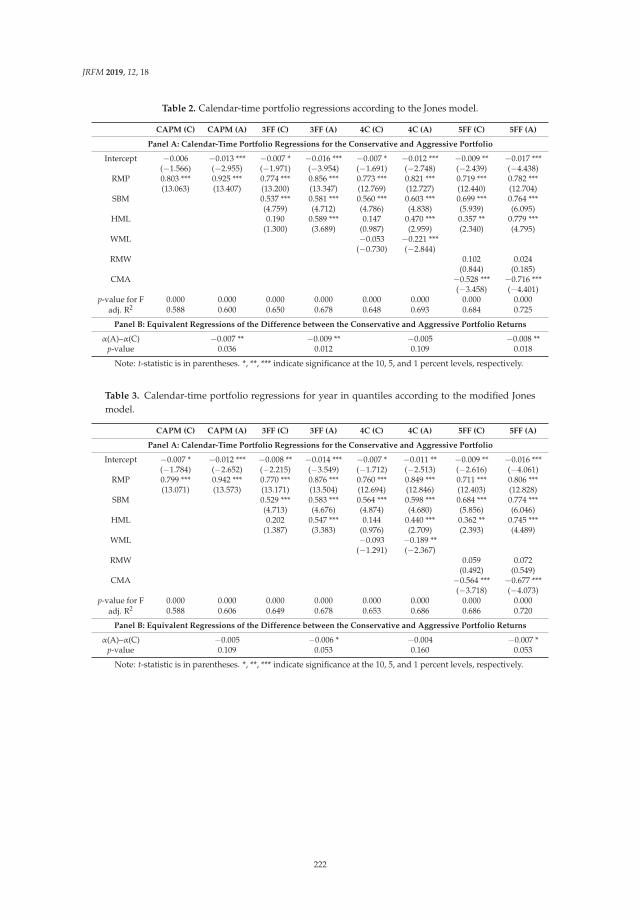
JRFM 2019, 12, 18
Table 2. Calendar-time portfolio regressions according to the Jones model.
CAPM (C) CAPM (A) 3FF (C) 3FF (A) 4C (C) 4C (A) 5FF (C) 5FF (A)
Panel A: Calendar-Time Portfolio Regressions for the Conservative and Aggressive Portfolio
Intercept −0.006 −0.013 *** −0.007 * −0.016 *** −0.007 * −0.012 *** −0.009 ** −0.017 ***(−1.566) (−2.955) (−1.971) (−3.954) (−1.691) (−2.748) (−2.439) (−4.438)
RMP 0.803 *** 0.925 *** 0.774 *** 0.856 *** 0.773 *** 0.821 *** 0.719 *** 0.782 ***(13.063) (13.407) (13.200) (13.347) (12.769) (12.727) (12.440) (12.704)
SBM 0.537 *** 0.581 *** 0.560 *** 0.603 *** 0.699 *** 0.764 ***(4.759) (4.712) (4.786) (4.838) (5.939) (6.095)
HML 0.190 0.589 *** 0.147 0.470 *** 0.357 ** 0.779 ***(1.300) (3.689) (0.987) (2.959) (2.340) (4.795)
WML −0.053 −0.221 ***(−0.730) (−2.844)
RMW 0.102 0.024(0.844) (0.185)
CMA −0.528 *** −0.716 ***(−3.458) (−4.401)
p-value for F 0.000 0.000 0.000 0.000 0.000 0.000 0.000 0.000adj. R2 0.588 0.600 0.650 0.678 0.648 0.693 0.684 0.725
Panel B: Equivalent Regressions of the Difference between the Conservative and Aggressive Portfolio Returns
α(A)–α(C) −0.007 ** −0.009 ** −0.005 −0.008 **p-value 0.036 0.012 0.109 0.018
Note: t-statistic is in parentheses. *, **, *** indicate significance at the 10, 5, and 1 percent levels, respectively.
Table 3. Calendar-time portfolio regressions for year in quantiles according to the modified Jonesmodel.
CAPM (C) CAPM (A) 3FF (C) 3FF (A) 4C (C) 4C (A) 5FF (C) 5FF (A)
Panel A: Calendar-Time Portfolio Regressions for the Conservative and Aggressive Portfolio
Intercept −0.007 * −0.012 *** −0.008 ** −0.014 *** −0.007 * −0.011 ** −0.009 ** −0.016 ***(−1.784) (−2.652) (−2.215) (−3.549) (−1.712) (−2.513) (−2.616) (−4.061)
RMP 0.799 *** 0.942 *** 0.770 *** 0.876 *** 0.760 *** 0.849 *** 0.711 *** 0.806 ***(13.071) (13.573) (13.171) (13.504) (12.694) (12.846) (12.403) (12.828)
SBM 0.529 *** 0.583 *** 0.564 *** 0.598 *** 0.684 *** 0.774 ***(4.713) (4.676) (4.874) (4.680) (5.856) (6.046)
HML 0.202 0.547 *** 0.144 0.440 *** 0.362 ** 0.745 ***(1.387) (3.383) (0.976) (2.709) (2.393) (4.489)
WML −0.093 −0.189 **(−1.291) (−2.367)
RMW 0.059 0.072(0.492) (0.549)
CMA −0.564 *** −0.677 ***(−3.718) (−4.073)
p-value for F 0.000 0.000 0.000 0.000 0.000 0.000 0.000 0.000adj. R2 0.588 0.606 0.649 0.678 0.653 0.686 0.686 0.720
Panel B: Equivalent Regressions of the Difference between the Conservative and Aggressive Portfolio Returns
α(A)–α(C) −0.005 −0.006 * −0.004 −0.007 *p-value 0.109 0.053 0.160 0.053
Note: t-statistic is in parentheses. *, **, *** indicate significance at the 10, 5, and 1 percent levels, respectively.
222

JRFM 2019, 12, 18
Table 4. Calendar-time portfolio regressions for year in quantiles according to the McNichols model.
CAPM (C) CAPM (A) 3FF (C) 3FF (A) 4C (C) 4C (A) 5FF (C) 5FF (A)
Panel A: Calendar-Time Portfolio Regressions for the Conservative and Aggressive Portfolio
Intercept −0.009 ** −0.011 ** −0.010 ** −0.013 *** −0.008 ** −0.010 ** −0.011 *** −0.015 ***(−2.147) (−2.579) (−2.602) (−3.388) (−2.010) (−2.463) (−3.065) (−4.032)
RMP 0.897 *** 0.827 *** 0.865 *** 0.771 *** 0.853 *** 0.749 *** 0.795 *** 0.710 ***(13.995) (12.905) (14.025) (12.749) (13.478) (12.139) (13.342) (12.103)
SBM 0.533 *** 0.529 *** 0.562 *** 0.549 *** 0.704 *** 0.729 ***(4.498) (4.551) (4.598) (4.605) (5.792) (6.098)
HML 0.229 0.463 *** 0.163 0.374 ** 0.422 *** 0.663 ***(1.488) (3.075) (1.049) (2.466) (2.681) (4.283)
WML −0.106 −0.156 **(−1.396) (−2.105)
RMW 0.057 0.141(0.459) (1.155)
CMA −0.678 *** −0.572 ***(−4.304) (−3.691)
p-value for F 0.000 0.000 0.000 0.000 0.000 0.000 0.000 0.000adj. R2 0.621 0.582 0.673 0.652 0.675 0.659 0.716 0.696
Panel B: Equivalent Regressions of the Difference between the Conservative and Aggressive Portfolio Returns
α(A)–α(C) −0.002 −0.003 −0.002 −0.003p-value 0.304 0.212 0.332 0.176
Note: t-statistic is in parentheses. *, **, *** indicate significance at the 10, 5, and 1 percent levels, respectively.
Table 5. Calendar-time portfolio regressions for year in quantiles according to the Ball–Shivakumarmodel.
CAPM (C) CAPM (A) 3FF (C) 3FF (A) 4C (C) 4C (A) 5FF (C) 5FF (A)
Panel A: Calendar-time portfolio regressions for the conservative and aggressive portfolio
Intercept −0.008 * −0.012 *** −0.009 ** −0.015 *** −0.008 * −0.012 *** −0.010 *** −0.016 ***(−1.810) (−2.953) (−2.222) (−3.965) (−1.737) (−2.908) (−2.632) (−4.526)
RMP 0.851 *** 0.884 *** 0.818 *** 0.822 *** 0.809 *** 0.797 *** 0.750 *** 0.762 ***(12.922) (13.584) (12.790) (13.790) (12.296) (13.148) (12.020) (13.140)
SBM 0.515 *** 0.611 *** 0.543 *** 0.629 *** 0.683 *** 0.794 ***(4.186) (5.334) (4.276) (5.375) (5.371) (6.718)
HML 0.237 0.511 *** 0.179 0.409 *** 0.428 ** 0.683 ***(1.488) (3.441) (1.106) (2.742) (2.594) (4.460)
WML −0.092 −0.177 **(−1.163) (−2.421)
RMW 0.060 0.095(0.462) (0.787)
CMA −0.659 *** −0.565 ***(−3.995) (−3.683)
p-value for F 0.000 0.000 0.000 0.000 0.000 0.000 0.000 0.000adj. R2 0.582 0.607 0.632 0.692 0.634 0.700 0.675 0.729
Panel B: Equivalent regressions of the difference between the conservative and aggressive portfolio returns
α(A)–α(C) −0.005 −0.006 * −0.004 −0.006 *p-value 0.120 0.071 0.173 0.071
Note: t-statistic is in parentheses. *, **, *** indicate significance at the 10, 5, and 1 percent levels, respectively.
223
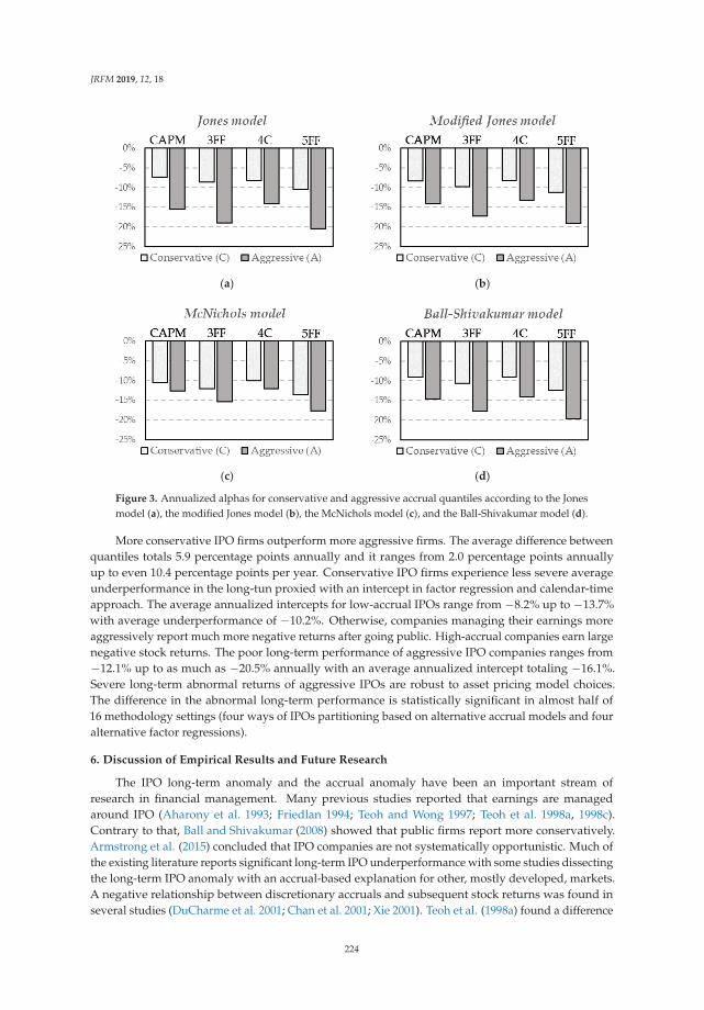
JRFM 2019, 12, 18
(a) (b)
(c) (d)
Figure 3. Annualized alphas for conservative and aggressive accrual quantiles according to the Jonesmodel (a), the modified Jones model (b), the McNichols model (c), and the Ball-Shivakumar model (d).
More conservative IPO firms outperform more aggressive firms. The average difference betweenquantiles totals 5.9 percentage points annually and it ranges from 2.0 percentage points annuallyup to even 10.4 percentage points per year. Conservative IPO firms experience less severe averageunderperformance in the long-tun proxied with an intercept in factor regression and calendar-timeapproach. The average annualized intercepts for low-accrual IPOs range from −8.2% up to −13.7%with average underperformance of −10.2%. Otherwise, companies managing their earnings moreaggressively report much more negative returns after going public. High-accrual companies earn largenegative stock returns. The poor long-term performance of aggressive IPO companies ranges from−12.1% up to as much as −20.5% annually with an average annualized intercept totaling −16.1%.Severe long-term abnormal returns of aggressive IPOs are robust to asset pricing model choices.The difference in the abnormal long-term performance is statistically significant in almost half of16 methodology settings (four ways of IPOs partitioning based on alternative accrual models and fouralternative factor regressions).
6. Discussion of Empirical Results and Future Research
The IPO long-term anomaly and the accrual anomaly have been an important stream ofresearch in financial management. Many previous studies reported that earnings are managedaround IPO (Aharony et al. 1993; Friedlan 1994; Teoh and Wong 1997; Teoh et al. 1998a, 1998c).Contrary to that, Ball and Shivakumar (2008) showed that public firms report more conservatively.Armstrong et al. (2015) concluded that IPO companies are not systematically opportunistic. Much ofthe existing literature reports significant long-term IPO underperformance with some studies dissectingthe long-term IPO anomaly with an accrual-based explanation for other, mostly developed, markets.A negative relationship between discretionary accruals and subsequent stock returns was found inseveral studies (DuCharme et al. 2001; Chan et al. 2001; Xie 2001). Teoh et al. (1998a) found a difference
224
JRFM 2019, 12, 18
in performance between aggressive and conservative firms and reported that more conservative firmsoutperformed more aggressive firms in the long-term. They concluded that the long-term returns rangefrom −2.23 percent to +0.94 percent per year for conservative IPOs. For aggressive IPOs, annualizedintercepts imply a long-term underperformance of −6.85 percent to −10.73 percent per year. The laststudy is especially important in discussing our results as it was also based on the calendar-timeportfolio approach. However, they tested the issue for US IPOs.
Taking together our results from the broad set of methodology settings, the conclusions about thesevere underperformance of aggressive IPOs are consentaneous and robust to methodology. The resultson the difference between conservative and aggressive IPOs based on a broad set of robustness checksof the calendar-time portfolio approach seem to support the conclusion about the negative relationshipbetween around-the-issue earnings management and subsequent long-term performance of IPOs.The annualized differences in alphas between conservative and aggressive initial public offerings inPoland are economically significant in all of the cases and they are statistically significant in almosthalf of 16 methodology settings. However, in some settings the difference is not statistically significantso the evidence on the explanatory power of earnings management for the long-term IPO returns inPoland may be perceived as not undisputable.
The results for Poland may be specific to some extent. First, the sample period includes substantialchanges of the capital market. This country has been classified as an emerging market by all of theleading agencies. Just recently, though, Poland has been ranked by FTSE Russell as a developed market.Ongoing improvements in Poland’s capital markets infrastructure and steady economic progress werethe key points of the decision. Simultaneously, Poland is still perceived as an emerging market byother agencies. Poland is an important area of economic growth in Europe. Poland’s economy wasthe only one in the European Union to avoid a recession through the last global financial crisis from2008–2009. It has been one of the largest economies in Europe. In the same time, Polish companies’capitalization as well as the number of equities listed on the exchange is much smaller in comparisonto US or other developed stock markets.
An important fact is that Poland has different characteristics to other markets. First, a simplecomparison to results for emerging markets is difficult because of the process of recent development inPoland. Second, a direct comparison to US-centered research or studies focused on other developedmarkets is also limited. Finally, one of the key fundamentals of capital market development arecorporate governance mechanisms which are crucial for its growth and stability (Brown et al. 2011;Krishnan et al. 2011; Hong et al. 2016). The area of corporate governance and corporate socialresponsibility as an extension of earnings management problem could be developed in future studies.The research on earnings manipulation around going public could also be broadened by the analysisof the role of insiders and institutional holdings in earnings manipulation around equity issues(Darrough and Rangan 2005; Wu and Yang 2018).
An important and pervasive issue in empirical corporate finance is endogeneity. It is mainlyconnected with the problem of correlation between explanatory variables and the error term ina regression. We do not apply a traditional regression model with earnings management asan explanatory variable and the subsequent long-term IPO performance as dependent variable.We use a different methodology which tests abnormal returns for IPO quantiles distinguisheddepending on the level of earnings management. Hence, the methods like instrumental variables,difference-in-difference method, or regression discontinuity design (Roberts and Whited 2005; Li 2016)have no direct application in our study. Another issue is the problem of endogenous events. We followDahlquist and Jong (2008) who demonstrate that the calendar-time approach is not biased and doesnot suffer from the problems of traditional measures of abnormal returns, even in small samples.They also report that it is unlikely that the endogeneity of clustering of IPOs explains the long-termunderperformance. The problem of testing endogenous events (not only IPOs) for small capitalmarkets like Warsaw Stock Exchange in Poland, could be developed in a separate study in the futureto continue the discussion of Schultz (2003), Viswanathan and Wei (2008), or Ang and Zhang (2015).
225

JRFM 2019, 12, 18
The issue of earnings management around initial public offerings is such a broad area of financialmanagement that this study was not able to answer all of the arising questions. Hence, the empiricalresearch could be extended in the future also in another way. One of the challenging directionsof future research is connected with real activities manipulation around the date of going public.Influencing the level of abnormal discretionary expenses and sales-based items is an example of realactivities manipulation. As the information set about market newcomers is usually limited, testingreal activities manipulation is not an easy task, especially for relatively small exchanges and thosethat have been classified as emerging markets for a long time. There exist studies where the realactivities manipulation has been tested in other settings, not especially connected with initial publicofferings (Graham et al. 2005; Roychowdhury 2006; Cohen and Zarowin 2010; Kothari et al. 2016).Earnings management through real activities around IPO has been discussed in a limited settingso far (Alhadab and Clacher 2018; Wongsunwai 2013). This study could also be continued byanalyzing the trade-off decision between real and accrual-based earnings manipulation (Zang 2012;Kothari et al. 2016). Another contributing research question would be to test whether IPO companies inPoland that managed accruals might have incentives to switch to real activities manipulation activities(Gunny 2010). Possible conclusions based on real activities management around going public wouldbe important for both investors and academics. The possible future research directions connected withempirical testing of real activities management could help shed new light on possible consequencesfor the long-term market IPO valuation.
7. Conclusions
We provide new evidence on the relationship between around-the-issue earnings managementand the long-term performance of initial public offerings (IPO) in Poland. We test this issue with amethodology that has not hitherto been applied for equities listed on the Warsaw Stock Exchange (WSE).The study gives international insights in the area of financial management, where country-specificfactors may influence managers’ decisions to manipulate earnings.
The results of testing the long-term implications of earnings management are important bothfor investors and academics. The informativeness of financial reports has always been of a greatimportance to investors. Earnings quality is an important practical concern during the whole lifeof companies, but it is of enormous importance around important company events such as goingpublic, when little is usually known about a company. As the information about earnings is key inevaluating the future prospects of a company and determining its value, managers have incentives tomanage earnings for that moment. If buyers are misled by artificially inflated earnings, they could paytoo high a price at IPO and suffer losses in the long-term when prices adjust to the real value of themarket newcomers.
Accrual quantiles are built using a set of alternative proxies of earnings management.The industry-year cross-sectional regressions are run for each IPO according to four models: the Jonesmodel, the modified Jones model, the McNichols model, and Ball–Shivakumar model. The long-termperformance is tested in 36-month rolling IPO portfolios under four asset pricing models: the CAPM,the Fama-French three-factor model, the Carhart four-factor model, and the Fama-French five-factormodel. The magnitude of IPO negative returns is sensitive to the methodology, but this does notchange the conclusions about long-term IPO underperformance. Both conservative and aggressivecompanies experience a relative decline in market value in the long run. However, we report moresevere long-term performance for accrual-aggressive IPO issuers, as the annualized abnormal returnsrange from −12.1% up to even −20.5%, whereas the span is −8.2% to −13.7% for conservative IPOcompanies. The average annualized intercepts for low-accrual IPOs is −10.2%. The poor long-termperformance of aggressive IPO companies is much more pronounced, as the average annualizedintercept totals −16.1%. This results for accrual quantiles are robust with respect to alternative accrualmodel specifications, and to alternative abnormal returns measures based on a set of factor models.The average difference in returns between quantiles totals 5.9 percentage points annually, and ranges
226

JRFM 2019, 12, 18
from 2.0 percentage points annually even up to 10.4 percentage points. Aggressive IPO companiesexperience more negative abnormal returns and this difference is economically significant in all ofthe cases. It is also statistically significant in almost half of methodology settings. The interpretationof such results could be as follows. Investors were not able to discount the pre-IPO use of abnormalaccruals. Following this, they were overoptimistic about the future prospects of the company. Once thetrue earnings performance is revealed over the course of time, they make downward price correctionsresulting in the negative long-term performance.
Author Contributions: The authors contributed equally to the research and writing of the manuscript.
Funding: Financial support for this paper from the National Science Centre, Poland is gratefully acknowledged(the number of the research project 2015/19/D/HS4/01950).
Acknowledgments: We would like to thank three anonymous referees.
Conflicts of Interest: The authors declare no conflict of interest. The funders had no role in the design of thestudy; in the collection, analyses, or interpretation of data; in the writing of the manuscript, or in the decision topublish the results.
References
Aharony, Joseph, Chan-Jane Lin, and Martin P. Loeb. 1993. Initial Public Offerings, Accounting Choices, andEarnings Management. Contemporary Accounting Research 10: 61–81. [CrossRef]
Ahmad-Zaluki, Nurwati A., Kevin Campbell, and Alan Goodacre. 2011. Earnings management in MalaysianIPOs: The East Asian crisis, ownership control, and post-IPO performance. International Journal of Accounting46: 111–37. [CrossRef]
Alhadab, Mohammad, and Iain Clacher. 2018. The impact of audit quality on real and accrual earningsmanagement around IPOs. British Accounting Review 50: 442–61. [CrossRef]
Ang, James S., and Shaojun Zhang. 2015. Evaluating Long-Horizon Event Study Methodology. In Handbookof Financial Econometrics and Statistics. Edited by Cheng-Few Lee and John C. Lee. New York: Springer,pp. 383–411.
Armstrong, Chris, George Foster, and Daniel J. Taylor. 2015. Abnormal accruals in newly public companies:Opportunistic misreporting or economic activity? Management Science 62: 1316–38. [CrossRef]
Ball, Ray, and Lakshmanan Shivakumar. 2005. Earnings quality in UK private firms: Comparative loss recognitiontimeliness. Journal of Accounting and Economics 39: 83–128. [CrossRef]
Ball, Ray, and Lakshmanan Shivakumar. 2006. The Role of Accruals in Asymmetrically Timely Gain and LossRecognition. Journal of Accounting Research 44: 207–42. [CrossRef]
Ball, Ray, and Lakshmanan Shivakumar. 2008. Earnings quality at initial public offerings. Journal of Accounting andEconomics 45: 324–49. [CrossRef]
Barber, Brad M., and John D. Lyon. 1997. Detecting long-run abnormal stock returns: The empirical power andspecification of test statistics. Journal of Financial Economics 43: 341–72. [CrossRef]
Beneish, Messod D. 1998. Discussion of “Are accruals during initial public offerings opportunistic?”. Review ofAccounting Studies 3: 209–21. [CrossRef]
Brown, Philip, Wendy Beekes, and Peter Verhoeven. 2011. Corporate governance, accounting and finance:A review. Accounting & Finance 51: 96–172. [CrossRef]
Carhart, Mark M. 1997. On Persistence in Mutual Fund Performance. Journal of Finance 52: 57–82. [CrossRef]Chan, Konan, Louis K. Chan, Narasimhan Jegadeesh, and Josef Lakonishok. 2001. Earnings quality and stock
returns. National Bureau of Economic Research. [CrossRef]Chen, Ken Y., Kuen-Lin Lin, and Jian Zhou. 2005. Audit quality and earnings management for Taiwan IPO firms.
Managerial Auditing Journal 20: 86–104. [CrossRef]Cohen, Daniel A., and Paul Zarowin. 2010. Accrual-based and real earnings management activities around
seasoned equity offerings. Journal of Accounting and Economics 50: 2–19. [CrossRef]Dahlquist, Magnus, and Frank de Jong. 2008. Pseudo Market Timing: A Reappraisal. Journal of Financial and
Quantitative Analysis 43: 547. [CrossRef]Darrough, Masako, and Srinivasan Rangan. 2005. Do Insiders Manipulate Earnings When They Sell Their Shares
in an Initial Public Offering? Journal of Accounting Research 43: 1–33. [CrossRef]
227

JRFM 2019, 12, 18
Dechow, Patricia M., and Ilia D. Dichev. 2002. The Quality of Accruals and Earnings: The Role of AccrualEstimation Errors. Accounting Review 77: 35–59. [CrossRef]
Dechow, Patricia M., Richard G. Sloan, and Amy P. Sweeney. 1995. Detecting Earnings Management. AccountingReview 70: 193–225. Available online: http://www.jstor.org/stable/248303 (accessed on 16 May 2015).
DeFond, Mark L., and James Jiambalvo. 1994. Debt covenant violation and manipulation of accruals. Journal ofAccounting and Economics 17: 145–76. [CrossRef]
DuCharme, Larry L., Paul H. Malatesta, and Stephan E. Sefcik. 2001. Earnings Management: IPO Valuation andSubsequent Performance. Journal of Accounting, Auditing & Finance 16: 369–96. [CrossRef]
Fama, Eugene F. 1998. Market efficiency, long-term returns, and behavioral finance. Journal of Financial Economics49: 283–306. [CrossRef]
Fama, Eugene F., and Kenneth R. French. 1993. Common risk factors in the returns on stocks and bonds. Journal ofFinancial Economics 33: 3–56. [CrossRef]
Fama, Eugene F., and Kenneth R. French. 2015. A five-factor asset pricing model. Journal of Financial Economics116: 1–22. [CrossRef]
Fama, Eugene F., and Kenneth R. French. 2016. Dissecting Anomalies with a Five-Factor Model. Review of FinancialStudies 29: 69–103. [CrossRef]
Friedlan, John M. 1994. Accounting Choices of Issuers of Initial Public Offerings. Contemporary Accounting Research11: 1–31. [CrossRef]
Gaver, Jennifer J., Kenneth M. Gaver, and Jeffrey R. Austin. 1995. Additional evidence on bonus plans and incomemanagement. Journal of Accounting and Economics 19: 3–28. [CrossRef]
Graham, John R., Campbell R. Harvey, and Shiva Rajgopal. 2005. The economic implications of corporate financialreporting. Journal of Accounting and Economics 40: 3–73. [CrossRef]
Gunny, Katherine A. 2010. The Relation Between Earnings Management Using Real Activities Manipulationand Future Performance: Evidence from Meeting Earnings Benchmarks. Contemporary Accounting Research27: 855–88. [CrossRef]
Healy, Paul M. 1985. The effect of bonus schemes on accounting decisions. Journal of Accounting and Economics7: 85–107. [CrossRef]
Holthausen, Robert W., David F. Larcker, and Richard G. Sloan. 1995. Annual bonus schemes and the manipulationof earnings. Journal of Accounting and Economics 19: 29–74. [CrossRef]
Hong, Bryan, Zhichuan Li, and Dylan Minor. 2016. Corporate Governance and Executive Compensation forCorporate Social Responsibility. Journal of Business Ethics 136: 199–213. [CrossRef]
Jegadeesh, Narasimhan, and Jason Karceski. 2009. Long-run performance evaluation: Correlation andheteroskedasticity-consistent tests. Journal of Empirical Finance 16: 101–11. [CrossRef]
Jones, Jennifer J. 1991. Earnings Management During Import Relief Investigations. Journal of Accounting Research29: 193–228. [CrossRef]
Kothari, Stephen P., Natalie Mizik, and Sugata Roychowdhury. 2016. Managing for the Moment: The Role ofEarnings Management via Real Activities versus Accruals in SEO Valuation. Accounting Review 91: 559–86.[CrossRef]
Krishnan, C. N. V., Vladimir I. Ivanov, Ronald W. Masulis, and Ajai K. Singh. 2011. Venture Capital Reputation,Post-IPO Performance, and Corporate Governance. Journal of Financial and Quantitative Analysis 46: 1295–333.[CrossRef]
Li, Frank. 2016. Endogeneity in CEO power: A survey and experiment. Investment Analysts Journal 45: 149–62.[CrossRef]
Liberty, Susan E., and Jerold L. Zimmerman. 1986. Labor union contract negotiations and accounting choices.Accounting Review 61: 692–712.
Lintner, John. 1969. The Valuation of Risk Assets and the Selection of Risky Investments in Stock Portfolios andCapital Budgets: A Reply. The Review of Economics and Statistics 51: 222–24. [CrossRef]
Lizinska, Joanna, and Leszek Czapiewski. 2018a. Earnings Management and the Long-Term Market Performanceof Initial Public Offerings in Poland. In Finance and Sustainability: Proceedings from the Finance and SustainabilityConference, Wroclaw 2017. Edited by Agnieszka Bem, Karolina Daszynska-Zygadło, Tat’ána Hajdíková andPéter Juhász. Springer Proceedings in Business and Economics. Cham: Springer International Publishing,vol. 62, pp. 121–34.
228

JRFM 2019, 12, 18
Lizinska, Joanna, and Leszek Czapiewski. 2018b. Towards Economic Corporate Sustainability in Reporting: WhatDoes Earnings Management around Equity Offerings Mean for Long-Term Performance? Sustainability10: 4349. [CrossRef]
Lyon, John D., Brad M. Barber, and Chih-Ling Tsai. 1999. Improved Methods for Tests of Long-Run AbnormalStock Returns. Journal of Finance 54: 165–201. [CrossRef]
McNichols, Maureen F. 2000. Research design issues in earnings management studies. Journal of Accounting andPublic Policy 19: 313–45. [CrossRef]
McNichols, Maureen F., and G. Peter Wilson. 1988. Evidence of Earnings Management from the Provision for BadDebts. Journal of Accounting Research 26: 1. [CrossRef]
Pastor-Llorca, María J., and Francisco Poveda-Fuentes. 2011. Earnings Management and the Long-RunPerformance of Spanish Initial Public Offerings. In Initial Public Offerings (IPO): An International Perspective ofIPOs. Edited by Greg N. Gregoriou. Quantitative Finance. Burlington: Elsevier Science, pp. 81–112.
Perry, Susan E., and Thomas H. Williams. 1994. Earnings management preceding management buyout offers.Journal of Accounting and Economics 18: 157–79. [CrossRef]
Pourciau, Susan. 1993. Earnings management and nonroutine executive changes. Journal of Accounting andEconomics 16: 317–36. [CrossRef]
Roberts, Michael R., and Toni M. Whited. 2005. Endogeneity in empirical corporate finance. Handbook of theEconomics of Finance 2: 493–572. [CrossRef]
Ronen, Joshua, and Varda Yaari. 2008. Earnings Management: Emerging Insights in Theory, Practice, and Research.Springer Series in Accounting Scholarship. New York: Springer.
Roosenboom, Peter, Tjalling van der Goot, and Gerard Mertens. 2003. Earnings management and initial publicofferings: Evidence from the Netherlands. International Journal of Accounting 38: 243–66. [CrossRef]
Roychowdhury, Sugata. 2006. Earnings management through real activities manipulation. Journal of Accountingand Economics 42: 335–70. [CrossRef]
Schultz, Paul. 2003. Pseudo Market Timing and the Long-Run Underperformance of IPOs. Journal of Finance58: 483–517. [CrossRef]
Sharpe, William F. 1964. Capital asset prices: A theory of market equilibrium under conditions of risk. Journal ofFinance 19: 425–42. [CrossRef]
Sloan, Richard G. 1996. Do stock prices fully reflect information in accruals and cash flows about future earnings?Accounting Review 71: 289–315.
Teoh, Siew Hong, Ivo Welch, and Tak J. Wong. 1998a. Earnings Management and the Long-Run MarketPerformance of Initial Public Offerings. Journal of Finance 53: 1935–74. [CrossRef]
Teoh, Siew Hong, Ivo Welch, and Tak J. Wong. 1998b. Earnings management and the underperformance ofseasoned equity offerings. Journal of Financial Economics 50: 63–99. [CrossRef]
Teoh, Siew Hong, Tak J. Wong, and Gita R. Rao. 1998c. Are Accruals during Initial Public Offerings Opportunistic?Review of Accounting Studies 3: 175–208. [CrossRef]
Teoh, Siew Hong, and Tak J. Wong. 1997. Analysts’ Credulity about Reported Earnings and Overoptimism inNew Equity Issues. SSRN Electronic Journal. [CrossRef]
Viswanathan, S., and Bin Wei. 2008. Endogenous Events and Long-Run Returns. Review of Financial Studies21: 855–88. [CrossRef]
Wongsunwai, Wan. 2013. The Effect of External Monitoring on Accrual-Based and Real Earnings Management:Evidence from Venture-Backed Initial Public Offerings. Contemporary Accounting Research 30: 296–324.[CrossRef]
Wu, Ching-Chih, and Tung-Hsiao Yang. 2018. Insider Trading and Institutional Holdings in Seasoned EquityOfferings. Journal of Risk and Financial Management 11: 53. [CrossRef]
Xie, Hong. 2001. The Mispricing of Abnormal Accruals. Accounting Review 76: 357–73. [CrossRef]Zang, Amy Y. 2012. Evidence on the Trade-Off between Real Activities Manipulation and Accrual-Based Earnings
Management. Accounting Review 87: 675–703. [CrossRef]
© 2019 by the authors. Licensee MDPI, Basel, Switzerland. This article is an open accessarticle distributed under the terms and conditions of the Creative Commons Attribution(CC BY) license (http://creativecommons.org/licenses/by/4.0/).
229
Journal of
Risk and FinancialManagement
Article
Effect of Corporate Governance on InstitutionalInvestors’ Preferences: An Empirical Investigationin Taiwan
Su-Lien Lu 1,* and Ying-Hui Li 2
1 International Bachelor Degree Program in Finance, National Pingtung University of Science and Technology,Neipu Pingtung 912, Taiwan
2 Graduate Institute of Finance, National Pingtung University of Science and Technology,Neipu Pingtung 912, Taiwan; [email protected]
* Correspondence: [email protected]
Received: 31 December 2018; Accepted: 10 February 2019; Published: 14 February 2019
Abstract: This study discusses the institutional investors’ shareholding base on corporate governancesystem in Taiwan. The sample was 4760 Taiwanese companies from 2005 to 2012. Then, this studyestablished six hypotheses to investigate the effects of corporate governance on institutional investors’shareholdings. The panel data regression model and piecewise regression model were adopted todetermine whether six hypotheses are supported. For sensitive analysis, additional considerationwas given on the basis of industrial category (electronics or nonelectronics), and the 2008–2010 globalfinancial crises. This study discovered that a nonlinear relationship exists between the domesticinstitutional investors’ shareholdings. The managerial ownership ratio and blockholder ownershipratio have positive effects both on domestic and foreign institutional investors. However, domesticand foreign institutional investors have distinct opinions regarding independent director ratios.Finally, the corporate governance did not improve institutional investors’ shareholdings duringfinancial crisis periods; instead, they paid more attention to firm profits or other characteristics.
Keywords: institutional investors’ shareholdings; panel data model; piecewise regression model;global financial crisis
1. Introduction
The Cadbury Report (Cadbury 1992) was first produced by the Committee on the FinancialAspects of Corporate Governance (Cadbury Committee), which provided the definition of corporategovernance as the “system by which companies are directed and controlled”, voluntary adoption of thegovernance best practices and the “comply or explain” principle (Shan and Napier 2014). The CadburyReport (Cadbury 1992) has proven important influences on development of corporate governancecodes worldwide.
The 1997 Asian financial crisis severely affected the economies of Southeast Asia because of theexit of foreign capital after property assets collapsed; this was a consequence of the lack of corporategovernance mechanisms in these countries. After the 1997 financial crisis in Asia, there are series ofcorporate fraud cases and distressed debt broke out in Taiwan. The Taiwanese government has beenpropagating the importance of corporate government to corporations since 1998.
In the United States, the 2001 Enron and Xerox cases led Congress to legislate the Sarbanes–OxleyAct to reinforce corporate governance in the United States. Therefore, corporate governance hasbecome a crucial subject garnering increased political interest. The passing of the law restored theaccuracy and reliability of financial information and established a series of requirements that affectedU.S. corporate governance and influenced similar laws in multiple countries, including Taiwan.
JRFM 2019, 12, 32; doi:10.3390/jrfm12010032 www.mdpi.com/journal/jrfm230
JRFM 2019, 12, 32
In 2006, Taiwanese government were legislated the Company Law and Securities and Exchange Act toempower corporate governance principles. Company Law is the regulation for corporate governance,including the operations of shareholders’ meetings, board of directors and supervisors. On 11 January2006, amendments to the Securities and Exchange Act were announced independent directors andaudit committees as well as to strength the function, structure and operations of a company’s boardof directors.
In 1999, the World Bank stated that corporate governance comprises internal and external aspects.Internal corporate governance, which involves monitoring activities and then taking corrective actionto accomplish organizational goals, facilitates internal monitoring by the board of directors. By contrast,external corporate governance involves externally monitoring manager behavior by including anindependent third party (i.e., an external auditor). Thus, corporate governance is a system of lawand sound approaches by which corporations are directed and controlled, focusing on internal andexternal corporate structures to monitor the actions of management and directors.
Jensen and Meckling (1976) discussed conflicts of interest between various contracting parties,including shareholders, corporate managers and debt holders. They found that agency costs generatedby the existence of debt and outside equity, which is the sum of monitoring costs, bonding costs andresidual loss. Fama and Jensen (1983) indicated corporate governance mechanisms are designed toreduce inefficiencies and eliminate agency costs.
Traditionally, institutional investors are passive owners and their growth will weaken governanceand exacerbate agency problems (Bebchuk et al. 2017). However, institutional investors are activeowners through proxy voting and behind-the-scenes engagement with management (Carleton et al.1998; McCahery et al. 2016; Appel et al. 2016). Thus, institutional investors with widespread holdingsmay benefit firms.
Aggarwal et al. (2005) suggested that obtaining high-quality accounting information enablesforeign investors to monitor and protect their investments and efficiently allocate capital. La Porta et al.(1997, 1998, 2000) indicated the necessity for strong investor protection laws and improved corporategovernance mechanisms that protect and attract outside investors. Elsewhere, Leuz et al. (2003)discovered that the quality of the information available for outside investors is also high in countrieswith strong investor protection laws; thus, the implementation of improved corporate governancemechanisms can attract institutional investors.
A substantial amount of research has explored the influence of corporate governance attributes oncorporate performance and has suggested that corporate governance variables significantly influencefirm performance. However, the relationship between corporate governance attributes and theinvestment preferences of institutional investors has seldom been discussed. This study contributes tothe literature by analyzing the relationship between the shareholding preferences of institutionalinvestors and corporate governance. This study establishes six hypotheses to investigate theshareholding preferences of domestic and foreign institutional investors based on corporate governancemechanisms, including managerial ownership, independent directors, blockholder ownership, pledgestock ratios and CEO duality. Then, the panel data regression model and piecewise regression modelare used to determine whether these hyphotheses are supported. The empirical results reveal thatcorporate governance variables have dissimilar effects on the investment preferences of domestic andforeign institutional investors, such as independent director ratio and pledge stock ratio. Moreover,a nonlinear relationship exists between the shareholding preferences of institutional investors andmanagerial ownership.
The remainder of this paper is organized as follows: Section 2 provides empirical designs,including hypotheses and definition of variables; Section 3 describes the details of the model, Section 4describes the data sample; Section 5 presents an analysis of the empirical results, and Section 6 presentsour conclusion.
231

JRFM 2019, 12, 32
2. Empirical Design
2.1. Hypotheses Development
Jensen and Meckling (1976) argued that managers are incentivized to seek pecuniary andnonpecuniary benefits at the expense of shareholder wealth. Managers divert progressively fewerfirm resources to nonvalue-maximizing activities when their equity stakes increase, because they mustbear an increasing fraction of agency costs associated with their expropriation activities. Therefore,managerial ownership may affect firm performance, which affects the shareholding preferences ofinstitutional investors. This study infers that managerial ownership has a positive relation withinstitutional investors’ shareholdings and establishes Hypothesis 1 as follows.
Hypothesis 1 (H1): The larger managerial ownership ratio, the higher institutional investors’ shareholdings.
However, the correlation between managerial ownership and firm performance is inconsistent.McConnell and Servaes (1990); Keasey et al. (1994) and Chen (2006) have all reported a bell-shapedrelationship between managerial ownership and firm performance. Conversely, Morck et al. (1988);Hermalin and Weisbach (1991); Mudambi and Nicosia (1998); Griffith (1999); Short and Keasey (1999);De Miguel et al. (2004); Florackis (2005) and Mura (2007) have observed a cubic relationship. Davieset al. (2005) and Florackis et al. (2009) have reported a quintic relationship. As a result, there is anonlinear relationship between managerial ownership and institutional investors’ shareholdings andHypothesis 2 was formulated as follows:
Hypothesis 2 (H2): The relationship between managerial ownership ratio and institutional investors’shareholdings is nonlinear.
The shareholding structure of a company can be divided into two categories, blockholder andnonblockholder, based on the percentage of shares owned. Because a high proportion of blockholderownership provides an excellent opportunity for management to optimize the company value,blockholder ownership may affect the participation of institutional investors. Driffield et al. (2007)revealed that the effects of blockholder ownership on company value are significant and positive in fourEast Asian countries. However, several studies have suggested that high blockholder ownership maydivert management action and harm minority shareholders; for example, Morck et al. (1988); Prowse(1993); Shleifer and Vishny (1997) and Minguez-Vera and Martin-Ugedo (2007) have determined thatblockholder effects tend to be negatively associated with firm performance. In summary, this studyinferred that the higher blockholder ownership, the higher the institutional investors’ shareholdings.Hypothesis 3 was established as follows.
Hypothesis 3 (H3): The higher blockholder ownership ratio, the greater institutional investors’ shareholdings.
The accounting scandals occurred primarily because of financial reporting fraud, includingnondisclosure and deliberate falsification. To reduce this risk and enhance the perceived integrity offinancial reports, the financial reports of a corporation must be audited by an independent externalauditor, who issues a report that accompanies the financial statements. A board includes internaland external directors. Fama and Jensen (1983) asserted that internal directors are likely to colludewith managers and make decisions against shareholders by exploiting their superior position andthe information that they can access. By contrast, external directors act as supervisors to eliminateproblems because of their neutral position. Beasley (1996) demonstrated that firms with independentdirectors have low scandal rates. If outside directors are independent and professionally capable, theycan objectively make decisions and effectively monitor managers. Weisbach (1988), Rosenstein andWyatt (1997) and Huson et al. (2001) have all reported that if a high ratio of independent directors arehired, firm performance improves. Thus, Hypothesis 4 was formulated as follows:
232
JRFM 2019, 12, 32
Hypothesis 4 (H4): The higher independent directors ratio, the higher institutional investors’ shareholdings.
Generally, directors can collateralize their shares and further purchase stocks to manipulate stockprices or enhance their power. Because the collateralized shares are closely related to share prices, thevalue of the collateralized shares depreciates when share prices slump. Consequently, shareholderswho collateralize their shares may prey on small shareholders or hurt the company. Kao et al. (2004)revealed that financial distress is closely related to high share ratios pledged by directors. Yeh andLee (2002) indicated that the higher the ratio of collateralized shares, the less favorable the firm’sperformance. Additionally, Chiou et al. (2002) discovered that if the proportion of shares collateralizedby a board of directors is high, the directors may be distracted from operating the business (becausethe fluctuation of stock prices is closely related to their finances), which leads to poor firm performance.Therefore, Hypothesis 5 was formulated as follows:
Hypothesis 5 (H5): The higher the collateralized shares by directors, the lower institutional investor’shareholdings.
The CEO is simultaneously the chairperson of the board, a practice that is common in the UnitedStates. From 1999 to 2003, a dual CEO leadership structure was applied in multiple firms that originallycomprised nondual structures. This trend partially stemmed from several high-profile cases involvingcompanies with dual CEO structures. However, the empirical evidence is inconsistent regarding whichleadership structure is more beneficial for firm performance. For example, Fama and Jensen (1983)and Jensen (1993) have reported that CEO duality may increase the expenses of an agency because theability of the board is hindered. Moreover, the weakening of a board’s ability to minimize the expensesof an agency can result in poor corporate performance (Jensen and Meckling 1976; Fama and Jensen1983; Patton and Baker 1987). Daily and Dalton (1993); Pi and Timme (1993) and Dahya et al. (1996)have all similarly suggested that CEO duality negatively affects the performance of a firm. However,U.S. regulators and investors are increasingly recommending against the separation of CEO andchairperson duties. Stoeberl and Sherony (1985) have suggested that dividing CEO and chairperson ofthe board duties may increase information-sharing costs, which can increase the communication costsof firm-specific information, decision-making processes, and other activities that are already inefficient.Assigning blame for poor company performance may also be more difficult with two leaders thanwhen there is only one. In the United Kingdom, Dahya et al. (2009) argued that the separation ofCEO and chairperson of the board duties cannot improve firm performance. Elsewhere, Boyd (1995)and Dahya and Travlos (2000) have documented a positive association between CEO duality and firmperformance. Although the specific effects remain unknown, it is clear that CEO duality influencesfirm performance, which affects the shareholdings of institutional investors. Accordingly, Hypothesis6 were formulated as follows:
Hypothesis 6 (H6): The higher CEO duality, the lower institutional investors’ shareholdings.
2.2. Variables Definitions
The shareholding preference of institutional investors (RELWEIGHT) was measured by the weightof their shareholding relative to their weight in the market. According to Zhang et al. (2009), theshareholding preference of institutional investors can be presented as:
RELWEIGHTjit =
WF,jit − WM
itWM
it, j = 1, 2; i = 1, . . . , N; t = 1, . . . , T (1)
where j = 1 and j = 2 represent domestic and foreign institutional investors, respectively; i denotes thefirm; t is the sample period from January 2005 to December 2012; and WM
it is the weight of firm i in the
233

JRFM 2019, 12, 32
market in period t. The expression WF,jit is the ratio of institutional investors’ shareholdings for firm i
in the market, and is defined by Zhang et al. (2009) as:
WF, jit =
INSTUjit × MVit
∑Ni=1 INSTUj
it × MVit(2)
where INSTUjit is the ratio of domestic or foreign shareholding of firm i in period t, and MVit is the
market value of firm i in period t.
3. Model
The data presented in this paper include time series and cross-sectional data that constitute apanel data model that refers to data sets consisting of multiple observations on each sampling unit.Panel data analysis was applied to investigate the investment preferences of domestic and foreigninvestors; this study also applied traditional ordinary least squares (OLS) for comparison.
Because the effects of managerial ownership on corporate performance represent a nonlinearrelationship, managerial ownership and institutional investors’ shareholdings may also be in anonlinear relationship. Therefore, this paper establishes two models. The first is constructed byassuming a linear relationship between investment preference and managerial ownership, whereasthe second model is a piecewise regression model constructed by assuming that three cutting pointsexist in a managerial ownership ratio. The first regression model is presented as
REALWEIGHTji,t
= β0 + β1MANAGERi,t−1 + β3 INDEPi,t−1 + β4PLEDGEi,t−1+β5DUALi,t−1 + β6LNTAi,t−1 + β7SYSTEMRISKi,t−1 + β8EPSi,t−1+νt
(3)
whereRELWEIGHT: institutional investors’ shareholdings.MANAGERi,t−1: managerial ownership ratio of firm i in period t − 1.BLOCKi,t−1: blockholder ownership of firm i in period t − 1. This variable is measured by
percentage in the top 5% by individual holding company and nonindividual nonholding company.INDEPi,t−1: independent director ratio of firm i in period t − 1.PLEDGEi,t−1: pledge stock ratio of firm i in period t − 1.DUALi,t−1: a dummy variable to measure whether the CEO is the chair of the board. This variable
is equal to 1 if the CEO is also the chair of the board; otherwise, it is 0.LNTAi,t−1: the firm scale of firm i in period t − 1, which is measured by taking the natural log of
total assets.SYSTEMRISKi,t−1: the system risk of firm i in period t − 1.EPSi,t−1: earning per share of firm i in period t − 1. This variable is measured asEPS = (Net Income − Preferred Dividends)/Weighted Average Number of Common
Shares OutstandingNotably, Equation (3) has three control variables: LNTA, SYSTEMRISK, and EPS. LNTA is the
natural log of total assets that is used to control the influence of firm scale measures on the shareholdingpreferences of institutional investors (Falkenstein 1996; Choe et al. 1999; Dahlquist and Robertsson2001; Gompers and Metrick 2001; Ng and Wang 2004). EPS is the proxy of firm performance used tocontrol the influence of firm performance measures on the shareholding preferences of institutionalinvestors (Faccio and Lasfer 1999). Finally, SYSTEMRISK is the market risk of sample firms, used tocontrol the influence of market risk measures on the shareholding preferences of institutional investors(Li 2002; Cao et al. 2007).
234

JRFM 2019, 12, 32
Morck et al. (1988) have demonstrated that managerial ownership is a crucial factor in regressionanalyses of firm performance. However, Morck et al. (1988); McConnell and Servaes (1990) andHolderness et al. (1999) have all discovered a substantial, inverse U-shaped relationship betweenmanagerial ownership and firm performance. Therefore, we considered managerial ownership to becrucial and nonmonotonical when evaluating the shareholdings of institutional investors. On the basisof Davies et al. (2005) and Zhang et al. (2009), we subsequently modified Equation (3) to a piecewiseregression model as follows:
RELWEIGHTji,t
= β0 + β1MANAGERi,t−1+β2(MANAGERi,t−1 − 10%)× a1
+β3(MANAGERi,t−1 − 20%)× a2
+β4(MANAGERi,t−1 − 30%)× a3 + β5BLOCKi,t−1+β6 INDEPi,t−1 + β7 PLEDGEi,t−1 + β8DUALi,t−1+β9LNTAi,t−1 + β10SYSTEMRISKi,t−1 + β11EPSi,t−1+νt
(4)
where
a1 =
{1, i f MANAGERi,t−1 ≥ 10%0, i f MANAGERi,t−1 < 10%
a2 =
{1, i f MANAGERi,t−1 ≥ 20%0, i f MANAGERi,t−1 < 20%
a3 =
{1, i f MANAGERi,t−1 ≥ 30%0, i f MANAGERi,t−1 < 30%
The definitions of other variables are defined in Equation (3).
4. Data
For the sample period from January 2005 to December 2012, this study collected 4760 samplesfrom 18 industries selected from among Taiwan’s listed companies.1 The sample period includethe 2007–2008 global financial crisis and apply the subsample period for sensitive analysis. Thesemonthly data obtained from the Taiwan Economic Journal (TEJ). However, this study excluded severalindustries, such as the financial and security industries, because of the sensitive nature of their business;incomplete data were also excluded.
5. Empirical Results and Analysis
5.1. Descriptive Statistics
Table 1 presents the descriptive statistics of the institutional investors’ shareholdings, corporatevariables and control variables. The mean of the managerial ownership ratio was 22.89%. However, themaximal value of the managerial ownership ratio was 89.24%, which was observed in the electronics
1 According to regulatory framework of corporate governance, which is shown by corporate governance center of TaiwanStock Exchange, the Taiwan Stock Exchange (TWSE) and Taipei Exchange (TPEx) specified their criteria for the reviewof securities listings in 2002. “An IPO company must set up an independent director and meet certain qualifications.Furthermore, regulations, such as ‘Corporate Governance Best Practice Principles’, ‘Code of Practice for Corporate SocialResponsibility’, and ‘Code of Practice for Integrity Management’ were subsequently announced for domestic enterprisesto follow. These will guide enterprises in strengthening their sense of corporate governance and social responsibility,establishing a consensus on integrity management, constructing a corporate governance culture, and creating mutualvalues.” (http://cgc.twse.com.tw/).
235
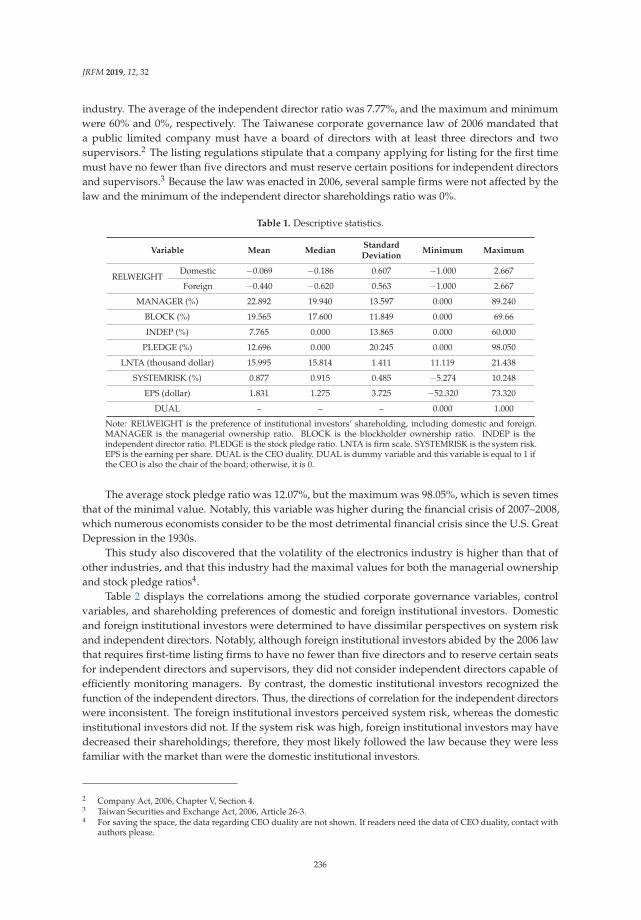
JRFM 2019, 12, 32
industry. The average of the independent director ratio was 7.77%, and the maximum and minimumwere 60% and 0%, respectively. The Taiwanese corporate governance law of 2006 mandated thata public limited company must have a board of directors with at least three directors and twosupervisors.2 The listing regulations stipulate that a company applying for listing for the first timemust have no fewer than five directors and must reserve certain positions for independent directorsand supervisors.3 Because the law was enacted in 2006, several sample firms were not affected by thelaw and the minimum of the independent director shareholdings ratio was 0%.
Table 1. Descriptive statistics.
Variable Mean MedianStandardDeviation
Minimum Maximum
RELWEIGHTDomestic −0.069 −0.186 0.607 −1.000 2.667
Foreign −0.440 −0.620 0.563 −1.000 2.667
MANAGER (%) 22.892 19.940 13.597 0.000 89.240
BLOCK (%) 19.565 17.600 11.849 0.000 69.66
INDEP (%) 7.765 0.000 13.865 0.000 60.000
PLEDGE (%) 12.696 0.000 20.245 0.000 98.050
LNTA (thousand dollar) 15.995 15.814 1.411 11.119 21.438
SYSTEMRISK (%) 0.877 0.915 0.485 −5.274 10.248
EPS (dollar) 1.831 1.275 3.725 −52.320 73.320
DUAL – – – 0.000 1.000
Note: RELWEIGHT is the preference of institutional investors’ shareholding, including domestic and foreign.MANAGER is the managerial ownership ratio. BLOCK is the blockholder ownership ratio. INDEP is theindependent director ratio. PLEDGE is the stock pledge ratio. LNTA is firm scale. SYSTEMRISK is the system risk.EPS is the earning per share. DUAL is the CEO duality. DUAL is dummy variable and this variable is equal to 1 ifthe CEO is also the chair of the board; otherwise, it is 0.
The average stock pledge ratio was 12.07%, but the maximum was 98.05%, which is seven timesthat of the minimal value. Notably, this variable was higher during the financial crisis of 2007–2008,which numerous economists consider to be the most detrimental financial crisis since the U.S. GreatDepression in the 1930s.
This study also discovered that the volatility of the electronics industry is higher than that ofother industries, and that this industry had the maximal values for both the managerial ownershipand stock pledge ratios4.
Table 2 displays the correlations among the studied corporate governance variables, controlvariables, and shareholding preferences of domestic and foreign institutional investors. Domesticand foreign institutional investors were determined to have dissimilar perspectives on system riskand independent directors. Notably, although foreign institutional investors abided by the 2006 lawthat requires first-time listing firms to have no fewer than five directors and to reserve certain seatsfor independent directors and supervisors, they did not consider independent directors capable ofefficiently monitoring managers. By contrast, the domestic institutional investors recognized thefunction of the independent directors. Thus, the directions of correlation for the independent directorswere inconsistent. The foreign institutional investors perceived system risk, whereas the domesticinstitutional investors did not. If the system risk was high, foreign institutional investors may havedecreased their shareholdings; therefore, they most likely followed the law because they were lessfamiliar with the market than were the domestic institutional investors.
2 Company Act, 2006, Chapter V, Section 4.3 Taiwan Securities and Exchange Act, 2006, Article 26-3.4 For saving the space, the data regarding CEO duality are not shown. If readers need the data of CEO duality, contact with
authors please.
236
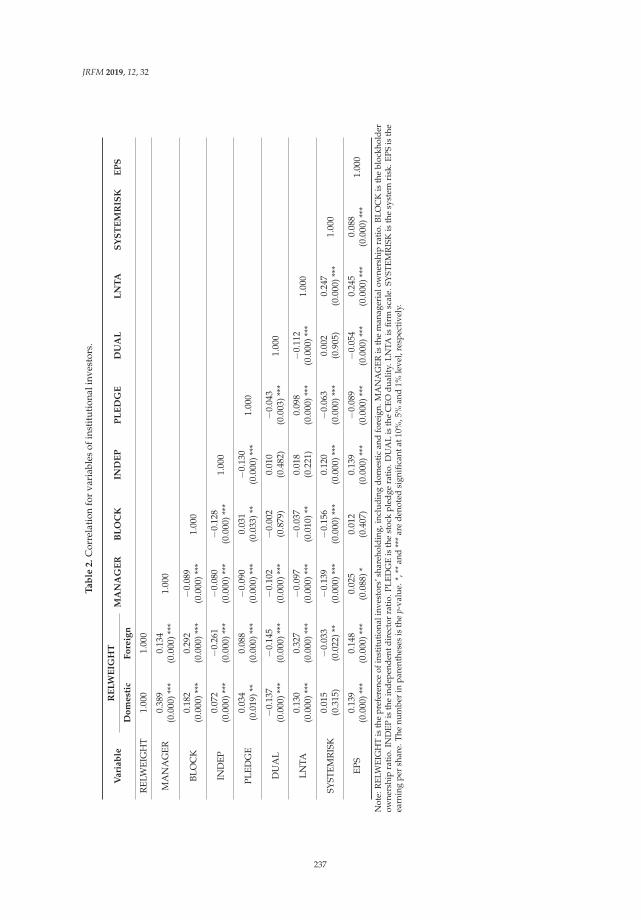
JRFM 2019, 12, 32
Ta
ble
2.
Cor
rela
tion
for
vari
able
sof
inst
itut
iona
linv
esto
rs.
Va
ria
ble
RE
LW
EIG
HT
MA
NA
GE
RB
LO
CK
IND
EP
PL
ED
GE
DU
AL
LN
TA
SY
ST
EM
RIS
KE
PS
Do
me
stic
Fo
reig
n
REL
WEI
GH
T1.
000
1.00
0
MA
NA
GER
0.38
9(0
.000
)***
0.13
4(0
.000
)***
1.00
0
BLO
CK
0.18
2(0
.000
)***
0.29
2(0
.000
)***
−0.0
89(0
.000
)***
1.00
0
IND
EP0.
072
(0.0
00)*
**−0
.261
(0.0
00)*
**−0
.080
(0.0
00)*
**−0
.128
(0.0
00)*
**1.
000
PLED
GE
0.03
4(0
.019
)**
0.08
8(0
.000
)***
−0.0
90(0
.000
)***
0.03
1(0
.033
)**
−0.1
30(0
.000
)***
1.00
0
DU
AL
−0.1
37(0
.000
)***
−0.1
45(0
.000
)***
−0.1
02(0
.000
)***
−0.0
02(0
.879
)0.
010
(0.4
82)
−0.0
43(0
.003
)***
1.00
0
LNTA
0.13
0(0
.000
)***
0.32
7(0
.000
)***
−0.0
97(0
.000
)***
−0.0
37(0
.010
)**
0.01
8(0
.221
)0.
098
(0.0
00)*
**−0
.112
(0.0
00)*
**1.
000
SYST
EMR
ISK
0.01
5(0
.315
)−0
.033
(0.0
22)*
*−0
.139
(0.0
00)*
**−0
.156
(0.0
00)*
**0.
120
(0.0
00)*
**−0
.063
(0.0
00)*
**0.
002
(0.9
05)
0.24
7(0
.000
)***
1.00
0
EPS
0.13
9(0
.000
)***
0.14
8(0
.000
)***
0.02
5(0
.088
)*0.
012
(0.4
07)
0.13
9(0
.000
)***
−0.0
89(0
.000
)***
−0.0
54(0
.000
)***
0.24
5(0
.000
)***
0.08
8(0
.000
)***
1.00
0
Not
e:R
ELW
EIG
HT
isth
epr
efer
ence
ofin
stitu
tiona
linv
esto
rs’s
hare
hold
ing,
incl
udin
gdo
mes
tican
dfo
reig
n.M
AN
AG
ERis
the
man
ager
ialo
wne
rshi
pra
tio.B
LOC
Kis
the
bloc
khol
der
owne
rshi
pra
tio.
IND
EPis
the
inde
pend
entd
irec
tor
rati
o.PL
EDG
Eis
the
stoc
kpl
edge
rati
o.D
UA
Lis
the
CEO
dual
ity.
LNTA
isfir
msc
ale.
SYST
EMR
ISK
isth
esy
stem
risk
.EPS
isth
eea
rnin
gpe
rsh
are.
The
num
ber
inpa
rent
hese
sis
the
p-va
lue.
*,**
and
***
are
deno
ted
sign
ifica
ntat
10%
,5%
and
1%le
vel,
resp
ecti
vely
.
237
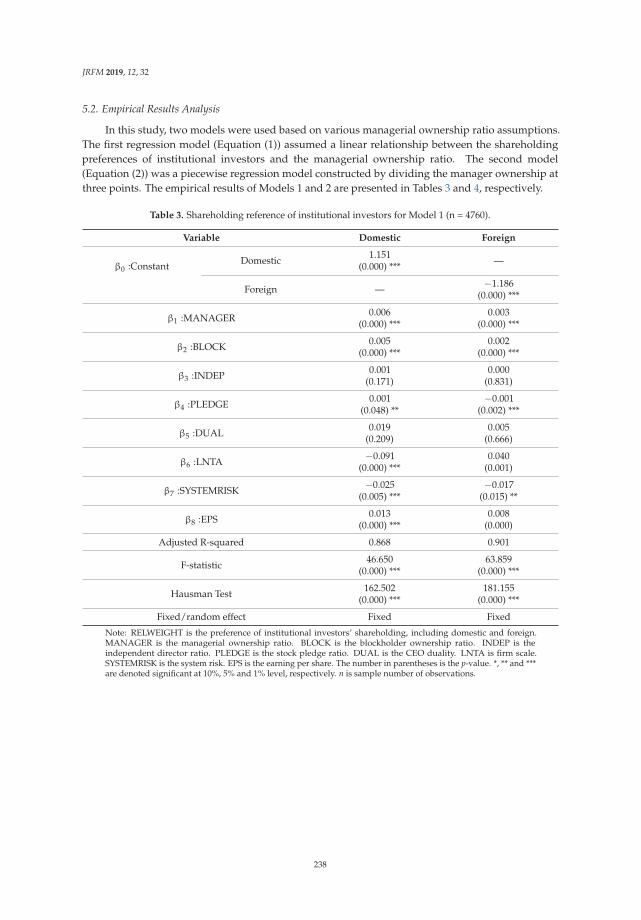
JRFM 2019, 12, 32
5.2. Empirical Results Analysis
In this study, two models were used based on various managerial ownership ratio assumptions.The first regression model (Equation (1)) assumed a linear relationship between the shareholdingpreferences of institutional investors and the managerial ownership ratio. The second model(Equation (2)) was a piecewise regression model constructed by dividing the manager ownership atthree points. The empirical results of Models 1 and 2 are presented in Tables 3 and 4, respectively.
Table 3. Shareholding reference of institutional investors for Model 1 (n = 4760).
Variable Domestic Foreign
β0 :Constant Domestic 1.151(0.000) *** —
Foreign — −1.186(0.000) ***
β1 :MANAGER 0.006(0.000) ***
0.003(0.000) ***
β2 :BLOCK 0.005(0.000) ***
0.002(0.000) ***
β3 :INDEP 0.001(0.171)
0.000(0.831)
β4 :PLEDGE 0.001(0.048) **
−0.001(0.002) ***
β5 :DUAL 0.019(0.209)
0.005(0.666)
β6 :LNTA −0.091(0.000) ***
0.040(0.001)
β7 :SYSTEMRISK −0.025(0.005) ***
−0.017(0.015) **
β8 :EPS 0.013(0.000) ***
0.008(0.000)
Adjusted R-squared 0.868 0.901
F-statistic 46.650(0.000) ***
63.859(0.000) ***
Hausman Test 162.502(0.000) ***
181.155(0.000) ***
Fixed/random effect Fixed Fixed
Note: RELWEIGHT is the preference of institutional investors’ shareholding, including domestic and foreign.MANAGER is the managerial ownership ratio. BLOCK is the blockholder ownership ratio. INDEP is theindependent director ratio. PLEDGE is the stock pledge ratio. DUAL is the CEO duality. LNTA is firm scale.SYSTEMRISK is the system risk. EPS is the earning per share. The number in parentheses is the p-value. *, ** and ***are denoted significant at 10%, 5% and 1% level, respectively. n is sample number of observations.
238
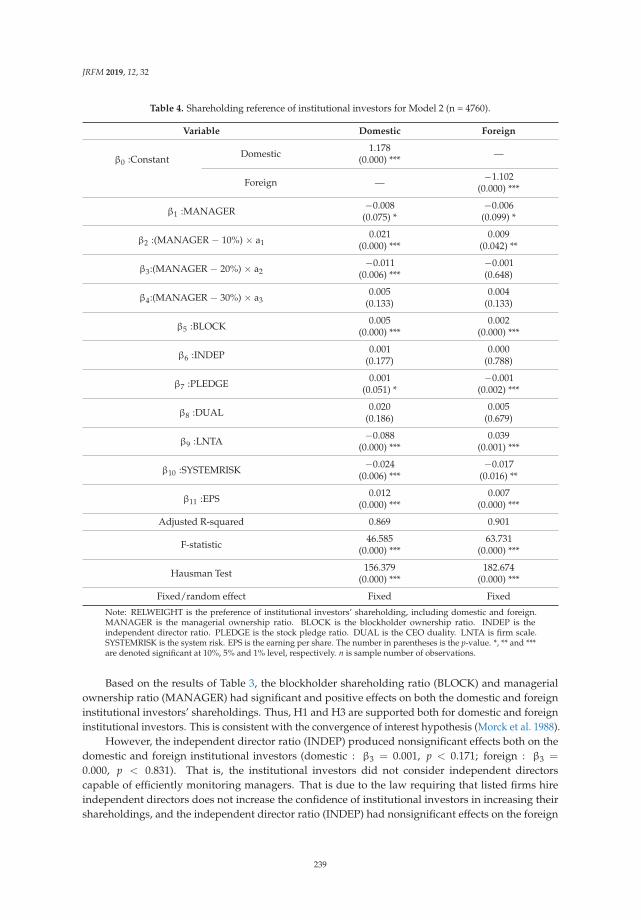
JRFM 2019, 12, 32
Table 4. Shareholding reference of institutional investors for Model 2 (n = 4760).
Variable Domestic Foreign
β0 :Constant Domestic 1.178(0.000) *** —
Foreign — −1.102(0.000) ***
β1 :MANAGER −0.008(0.075) *
−0.006(0.099) *
β2 :(MANAGER − 10%) × a10.021
(0.000) ***0.009
(0.042) **
β3:(MANAGER − 20%) × a2−0.011
(0.006) ***−0.001(0.648)
β4:(MANAGER − 30%) × a30.005
(0.133)0.004
(0.133)
β5 :BLOCK 0.005(0.000) ***
0.002(0.000) ***
β6 :INDEP 0.001(0.177)
0.000(0.788)
β7 :PLEDGE 0.001(0.051) *
−0.001(0.002) ***
β8 :DUAL 0.020(0.186)
0.005(0.679)
β9 :LNTA −0.088(0.000) ***
0.039(0.001) ***
β10 :SYSTEMRISK −0.024(0.006) ***
−0.017(0.016) **
β11 :EPS 0.012(0.000) ***
0.007(0.000) ***
Adjusted R-squared 0.869 0.901
F-statistic 46.585(0.000) ***
63.731(0.000) ***
Hausman Test 156.379(0.000) ***
182.674(0.000) ***
Fixed/random effect Fixed Fixed
Note: RELWEIGHT is the preference of institutional investors’ shareholding, including domestic and foreign.MANAGER is the managerial ownership ratio. BLOCK is the blockholder ownership ratio. INDEP is theindependent director ratio. PLEDGE is the stock pledge ratio. DUAL is the CEO duality. LNTA is firm scale.SYSTEMRISK is the system risk. EPS is the earning per share. The number in parentheses is the p-value. *, ** and ***are denoted significant at 10%, 5% and 1% level, respectively. n is sample number of observations.
Based on the results of Table 3, the blockholder shareholding ratio (BLOCK) and managerialownership ratio (MANAGER) had significant and positive effects on both the domestic and foreigninstitutional investors’ shareholdings. Thus, H1 and H3 are supported both for domestic and foreigninstitutional investors. This is consistent with the convergence of interest hypothesis (Morck et al. 1988).
However, the independent director ratio (INDEP) produced nonsignificant effects both on thedomestic and foreign institutional investors (domestic : β3 = 0.001, p < 0.171; foreign : β3 =
0.000, p < 0.831). That is, the institutional investors did not consider independent directorscapable of efficiently monitoring managers. That is due to the law requiring that listed firms hireindependent directors does not increase the confidence of institutional investors in increasing theirshareholdings, and the independent director ratio (INDEP) had nonsignificant effects on the foreign
239

JRFM 2019, 12, 32
institutional investors’ shareholdings. Therefore, H4 is not supported both for domestic and foreigninstitutional investors.
The stock pledge ratio (PLEDGE) has positive effect on domestic institutional investors’shareholdings (β4 = 0.001, p < 0.048 **), but has negative effect on foreign institutional investors(β4 = −0.001, p < 0.002 ∗∗∗). The foreign institutional investors may consider that when directorscollateralize shares and engage in over-leveraged transactions, the company may has higher risk.Therefore, H5 is only supported for foreign institutional investors.
The results for CEO duality are all nonsignificant (domestic: β5 = 0.019, p < 0.209; foreign : β5 =
0.005, p < 0.666) That is, whether or not the separation of CEO and chairperson of the board dutiescannot improve or decrease institutional investors’ shareholdings. Therefore, H6 is not supported bothfor domestic and foreign institutional investors.
From Table 3, the managerial ownership ratio has significant effects both on domestic and foreigninstitutional investors (domestic: β1 = 0.006, p < 0.000 ***; foreign: β1 = 0.003, p < 0.000 ***). Thedescriptive statistics table (Table 1) gave the mean of the managerial ownership ratio as 22%, thus,we divided the variable at three points, 10%, 20%, and 30%, to analyze the nonlinear relationshipbetween the shareholdings of institutional investors and the managerial ownership ratio using thepiecewise regression model. From Table 4, a nonlinear relationship was found between managerialshare ownership and institutional investors’ shareholdings; the latter decreased when the managerialownership ratios were between 20% and 30%. If the managerial ownership ratio larger than 10%, ithad positive effects on institutional investors’ shareholdings (domestic: β2 = 0.021, p < 0.000 ∗∗∗;foreigm: β2 = 0.009, p < 0.042 ∗∗). However, when the ratio increase to 20%, the effects will turn tonegative (domestic: β3 = −0.011, p < 0.006 ∗∗∗; foreigm: β3 = −0.001, p < 0.648), but the results forforeign institutional investors are nonsignificant. Consequently, H2 is only supported for domesticinstitutional investors.
5.3. Sensitive Analysis
5.3.1. Electronics and Nonelectronics Industry Analysis
Because half of the sampled firms are in the electronics industry, this study divided thesamples into two categories, electronics and nonelectronics industries, to analyze the behavior ofinstitutional investors.
The results of Model 1 for electronics and nonelectronics industries were shown in Tables 5and 6. Comparing Tables 5 and 6, this study found that the independent director ratio (INDEP) onlyhad a significant positive effect on the institutional investors for nonelectronics industry (domestic:β3 = 0.095, p < 0.080 ∗; foreign: β3 = 0.173, p < 0.003 ∗∗∗). This indicates that they observed the lawregarding listed firms and the hiring of independent directors. Further, most Taiwanese companies arefamily businesses, particularly in nonelectronics industries, where director and supervisor positionsare held by family members and ownership interest is concentrated in only a few shareholders. Thus,they mind the function of independent directors for nonelectronics industry. However, for electronicsindustry, the independent director ratio (INDEP) had nonsignificant effects both on domestic andforeign institutional investors (domestic: β3 = 0.001, p < 0.268; foreign: β3 = 0.000, p < 0.722).Consequently, H4 is only supported for nonelectronics industry.
240
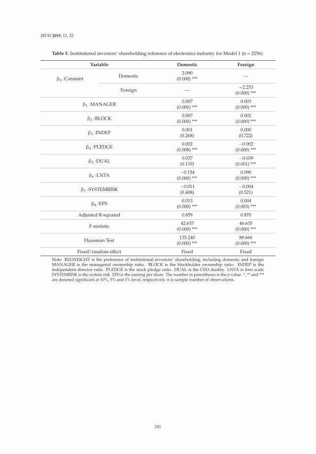
JRFM 2019, 12, 32
Table 5. Institutional investors’ shareholding reference of electronics industry for Model 1 (n = 2256).
Variable Domestic Foreign
β0 :Constant Domestic 2.090(0.000) *** —
Foreign — −2.253(0.000) ***
β1 :MANAGER 0.007(0.000) ***
0.003(0.000) ***
β2 :BLOCK 0.007(0.000) ***
0.002(0.000) ***
β3 :INDEP 0.001(0.268)
0.000(0.722)
β4 :PLEDGE 0.002(0.008) ***
−0.002(0.000) ***
β5 :DUAL 0.037(0.119)
−0.039(0.001) ***
β6 :LNTA −0.154(0.000) ***
0.090(0.000) ***
β7 :SYSTEMRISK −0.011(0.408)
−0.004(0.521)
β8 :EPS 0.013(0.000) ***
0.004(0.003) ***
Adjusted R-squared 0.859 0.870
F-statistic 42.637(0.000) ***
46.635(0.000) ***
Hausman Test 135.240(0.000) ***
88.666(0.000) ***
Fixed/random effect Fixed Fixed
Note: RELWEIGHT is the preference of institutional investors’ shareholding, including domestic and foreign.MANAGER is the managerial ownership ratio. BLOCK is the blockholder ownership ratio. INDEP is theindependent director ratio. PLEDGE is the stock pledge ratio. DUAL is the CEO duality. LNTA is firm scale.SYSTEMRISK is the system risk. EPS is the earning per share. The number in parentheses is the p-value. *, ** and ***are denoted significant at 10%, 5% and 1% level, respectively. n is sample number of observations.
241
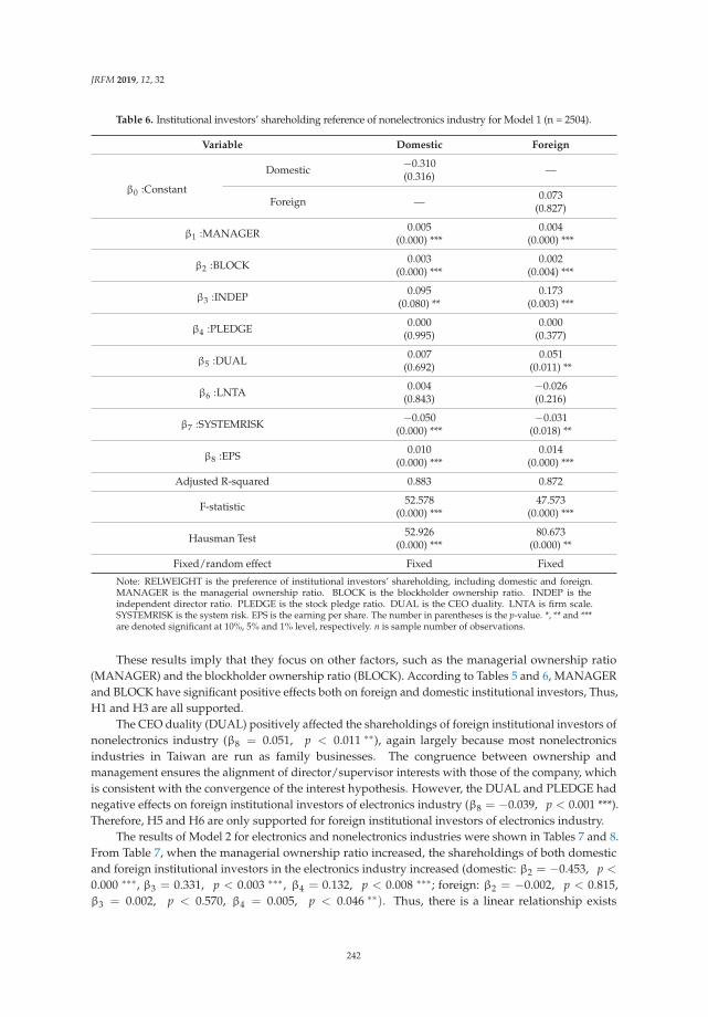
JRFM 2019, 12, 32
Table 6. Institutional investors’ shareholding reference of nonelectronics industry for Model 1 (n = 2504).
Variable Domestic Foreign
β0 :Constant
Domestic −0.310(0.316) —
Foreign — 0.073(0.827)
β1 :MANAGER 0.005(0.000) ***
0.004(0.000) ***
β2 :BLOCK 0.003(0.000) ***
0.002(0.004) ***
β3 :INDEP 0.095(0.080) **
0.173(0.003) ***
β4 :PLEDGE 0.000(0.995)
0.000(0.377)
β5 :DUAL 0.007(0.692)
0.051(0.011) **
β6 :LNTA 0.004(0.843)
−0.026(0.216)
β7 :SYSTEMRISK −0.050(0.000) ***
−0.031(0.018) **
β8 :EPS 0.010(0.000) ***
0.014(0.000) ***
Adjusted R-squared 0.883 0.872
F-statistic 52.578(0.000) ***
47.573(0.000) ***
Hausman Test 52.926(0.000) ***
80.673(0.000) **
Fixed/random effect Fixed Fixed
Note: RELWEIGHT is the preference of institutional investors’ shareholding, including domestic and foreign.MANAGER is the managerial ownership ratio. BLOCK is the blockholder ownership ratio. INDEP is theindependent director ratio. PLEDGE is the stock pledge ratio. DUAL is the CEO duality. LNTA is firm scale.SYSTEMRISK is the system risk. EPS is the earning per share. The number in parentheses is the p-value. *, ** and ***are denoted significant at 10%, 5% and 1% level, respectively. n is sample number of observations.
These results imply that they focus on other factors, such as the managerial ownership ratio(MANAGER) and the blockholder ownership ratio (BLOCK). According to Tables 5 and 6, MANAGERand BLOCK have significant positive effects both on foreign and domestic institutional investors, Thus,H1 and H3 are all supported.
The CEO duality (DUAL) positively affected the shareholdings of foreign institutional investors ofnonelectronics industry (β8 = 0.051, p < 0.011 ∗∗), again largely because most nonelectronicsindustries in Taiwan are run as family businesses. The congruence between ownership andmanagement ensures the alignment of director/supervisor interests with those of the company, whichis consistent with the convergence of the interest hypothesis. However, the DUAL and PLEDGE hadnegative effects on foreign institutional investors of electronics industry (β8 = −0.039, p < 0.001 ***).Therefore, H5 and H6 are only supported for foreign institutional investors of electronics industry.
The results of Model 2 for electronics and nonelectronics industries were shown in Tables 7 and 8.From Table 7, when the managerial ownership ratio increased, the shareholdings of both domesticand foreign institutional investors in the electronics industry increased (domestic: β2 = −0.453, p <
0.000 ∗∗∗, β3 = 0.331, p < 0.003 ∗∗∗, β4 = 0.132, p < 0.008 ∗∗∗; foreign: β2 = −0.002, p < 0.815,β3 = 0.002, p < 0.570, β4 = 0.005, p < 0.046 ∗∗). Thus, there is a linear relationship exists
242

JRFM 2019, 12, 32
between them. Thus, H2 were supported both for domestic and foreign institutional investors ofelectronics industry.
Table 7. Institutional investors’ shareholding reference of electronics industry for Model 2 (n = 2256).
Variable Domestic Foreign
β0 :Constant
Domestic 1982.901(0.000) *** —
Foreign — −2.150(0.000) ***
β1 :MANAGER −0.214(0.246)
0.002(0.806)
β2:(MANAGER − 10%) × a1 −0.453(0.000) ***
−0.002(0.815)
β3:(MANAGER − 20%) × a2 0.331(0.003) ***
0.002(0.570)
β4:(MANAGER − 30%) × a3 0.132(0.008) ***
0.005(0.046) **
β5 :BLOCK −0.019(0.630)
0.003(0.000) ***
β6 :INDEP 0.058(0.000) ***
0.000(0.582)
β7 :PLEDGE −0.043(0.000) ***
−0.001(0.000) ***
β8 :DUAL 0.005(0.262)
−0.041(0.001) ***
β9 :LNTA −0.091(0.627)
0.085(0.000) ***
β10 :SYSTEMRISK 1.941(0.000) ***
−0.004(0.505)
β11 :EPS −0.003(0.010) **
0.004(0.003) ***
Adjusted R-squared 0.033 0.871
F-statistic 1.230(0.008) ***
46.484(0.000) ***
Hausman Test 297.266(0.000) ***
101.735(0.000) ***
Fixed/random effect Fixed Fixed
Note: RELWEIGHT is the preference of institutional investors’ shareholding, including domestic and foreign.MANAGER is the managerial ownership ratio. BLOCK is the blockholder ownership ratio. INDEP is theindependent director ratio. PLEDGE is the stock pledge ratio. DUAL is the CEO duality. LNTA is firm scale.SYSTEMRISK is the system risk. EPS is the earning per share. The number in parentheses is the p-value. *, ** and ***are denoted significant at 10%, 5% and 1% level, respectively. n is sample number of observations.
243
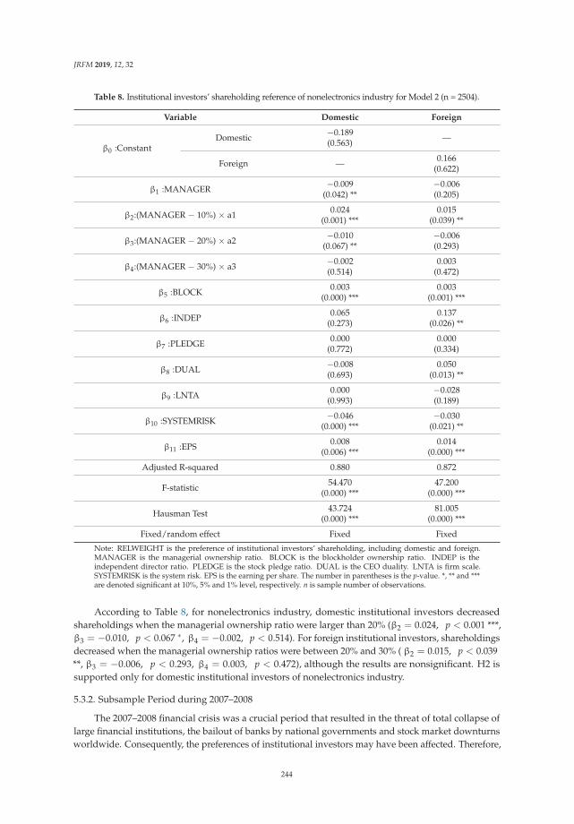
JRFM 2019, 12, 32
Table 8. Institutional investors’ shareholding reference of nonelectronics industry for Model 2 (n = 2504).
Variable Domestic Foreign
β0 :ConstantDomestic −0.189
(0.563) —
Foreign — 0.166(0.622)
β1 :MANAGER −0.009(0.042) **
−0.006(0.205)
β2:(MANAGER − 10%) × a1 0.024(0.001) ***
0.015(0.039) **
β3:(MANAGER − 20%) × a2 −0.010(0.067) **
−0.006(0.293)
β4:(MANAGER − 30%) × a3 −0.002(0.514)
0.003(0.472)
β5 :BLOCK 0.003(0.000) ***
0.003(0.001) ***
β6 :INDEP 0.065(0.273)
0.137(0.026) **
β7 :PLEDGE 0.000(0.772)
0.000(0.334)
β8 :DUAL −0.008(0.693)
0.050(0.013) **
β9 :LNTA 0.000(0.993)
−0.028(0.189)
β10 :SYSTEMRISK −0.046(0.000) ***
−0.030(0.021) **
β11 :EPS 0.008(0.006) ***
0.014(0.000) ***
Adjusted R-squared 0.880 0.872
F-statistic 54.470(0.000) ***
47.200(0.000) ***
Hausman Test 43.724(0.000) ***
81.005(0.000) ***
Fixed/random effect Fixed Fixed
Note: RELWEIGHT is the preference of institutional investors’ shareholding, including domestic and foreign.MANAGER is the managerial ownership ratio. BLOCK is the blockholder ownership ratio. INDEP is theindependent director ratio. PLEDGE is the stock pledge ratio. DUAL is the CEO duality. LNTA is firm scale.SYSTEMRISK is the system risk. EPS is the earning per share. The number in parentheses is the p-value. *, ** and ***are denoted significant at 10%, 5% and 1% level, respectively. n is sample number of observations.
According to Table 8, for nonelectronics industry, domestic institutional investors decreasedshareholdings when the managerial ownership ratio were larger than 20% (β2 = 0.024, p < 0.001 ***,β3 = −0.010, p < 0.067 ∗, β4 = −0.002, p < 0.514). For foreign institutional investors, shareholdingsdecreased when the managerial ownership ratios were between 20% and 30% ( β2 = 0.015, p < 0.039**, β3 = −0.006, p < 0.293, β4 = 0.003, p < 0.472), although the results are nonsignificant. H2 issupported only for domestic institutional investors of nonelectronics industry.
5.3.2. Subsample Period during 2007–2008
The 2007–2008 financial crisis was a crucial period that resulted in the threat of total collapse oflarge financial institutions, the bailout of banks by national governments and stock market downturnsworldwide. Consequently, the preferences of institutional investors may have been affected. Therefore,
244
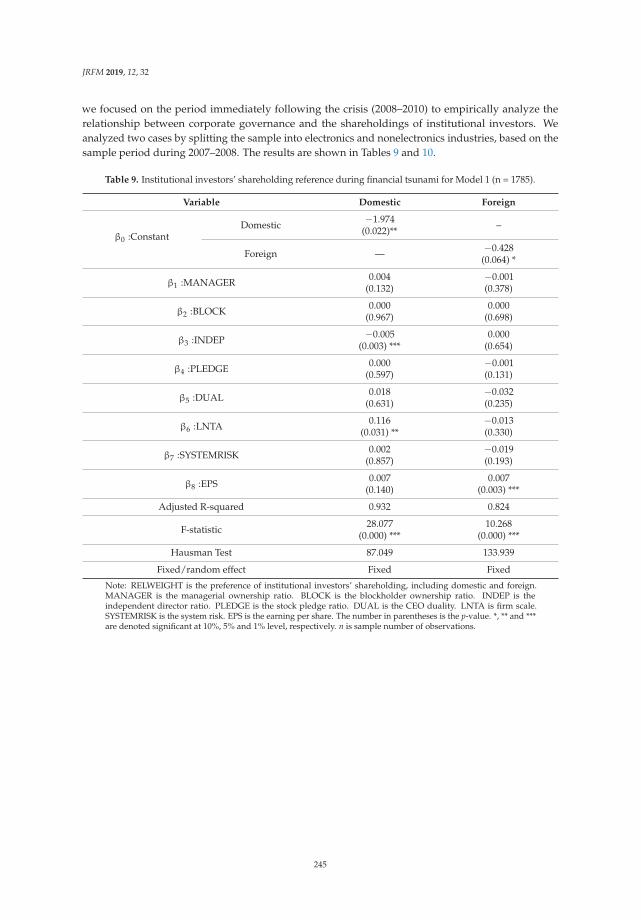
JRFM 2019, 12, 32
we focused on the period immediately following the crisis (2008–2010) to empirically analyze therelationship between corporate governance and the shareholdings of institutional investors. Weanalyzed two cases by splitting the sample into electronics and nonelectronics industries, based on thesample period during 2007–2008. The results are shown in Tables 9 and 10.
Table 9. Institutional investors’ shareholding reference during financial tsunami for Model 1 (n = 1785).
Variable Domestic Foreign
β0 :ConstantDomestic −1.974
(0.022)** –
Foreign — −0.428(0.064) *
β1 :MANAGER 0.004(0.132)
−0.001(0.378)
β2 :BLOCK 0.000(0.967)
0.000(0.698)
β3 :INDEP −0.005(0.003) ***
0.000(0.654)
β4 :PLEDGE 0.000(0.597)
−0.001(0.131)
β5 :DUAL 0.018(0.631)
−0.032(0.235)
β6 :LNTA 0.116(0.031) **
−0.013(0.330)
β7 :SYSTEMRISK 0.002(0.857)
−0.019(0.193)
β8 :EPS 0.007(0.140)
0.007(0.003) ***
Adjusted R-squared 0.932 0.824
F-statistic 28.077(0.000) ***
10.268(0.000) ***
Hausman Test 87.049 133.939
Fixed/random effect Fixed Fixed
Note: RELWEIGHT is the preference of institutional investors’ shareholding, including domestic and foreign.MANAGER is the managerial ownership ratio. BLOCK is the blockholder ownership ratio. INDEP is theindependent director ratio. PLEDGE is the stock pledge ratio. DUAL is the CEO duality. LNTA is firm scale.SYSTEMRISK is the system risk. EPS is the earning per share. The number in parentheses is the p-value. *, ** and ***are denoted significant at 10%, 5% and 1% level, respectively. n is sample number of observations.
245

JRFM 2019, 12, 32
Table 10. Institutional investors’ shareholding reference during financial tsunami for Model 2 (n = 1785).
Variable Domestic Foreign
β0 :ConstantDomestic −2.145
(0.017) ** —
Foreign — −2.397(0.000) ***
β1 :MANAGER 0.015(0.380)
0.005(0.688)
β2:(MANAGER − 10%) × a1 −0.012(0.545)
−0.003(0.829)
β3:(MANAGER − 20%) × a2 0.002(0.843)
0.001(0.904)
β4:(MANAGER − 30%) × a3 −0.003(0.760)
0.001(0.885)
β5 :BLOCK 0.000(0.965)
0.003(0.072) *
β6 :INDEP −0.005(0.003) ***
0.000(0.706)
β7 :PLEDGE 0.001(0.542)
0.000(0.802)
β8 :DUAL 0.018(0.647)
0.001(0.971)
β9 :LNTA 0.120(0.027) **
0.113(0.002) ***
β10 :SYSTEMRISK 0.003(0.843)
0.006(0.550)
β11 :EPS 0.006(0.163)
0.000(0.973)
Adjusted R-squared 0.932 0.960
F-statistic 27.822(0.000) ***
48.702(0.000) ***
Hausman Test 85.930(0.000) ***
93.116(0.000) ***
Fixed/random effect Fixed Fixed
Note: RELWEIGHT is the preference of institutional investors’ shareholding, including domestic and foreign.MANAGER is the managerial ownership ratio. BLOCK is the blockholder ownership ratio. INDEP is theindependent director ratio. PLEDGE is the stock pledge ratio. DUAL is the CEO duality. LNTA is firm scale.SYSTEMRISK is the system risk. EPS is the earning per share. The number in parentheses is the p-value. *, ** and ***are denoted significant at 10%, 5% and 1% level, respectively. n is sample number of observations.
From Table 9, domestic and foreign institutional investors valued the monitoring function ofindependent directors (β3 = −0.005, p < 0.003 ***). However, the independent director ratio (INDEP)did not improve foreign institutional investors’ investment confidence (β3 = 0.000, p < 0.654). Forother corportate governance variables, most estimated results are nonsignofcant, Consequently, H1,H3, H4, H5, and H6 are not supported.
According to Table 10, we discovered that the shareholdings of foreign institutionalinvestors uniformly increased as the managerial ownership ratio increased, but are nonsignificant(β2 = −0.003, p < 0.829; β3 = 0.001, p < 0.904; β4 = 0.001, p < 0.885). The managerialownership ratio also positively affected the shareholdings of domestic institutional investorswhen a manager owned 20% of the equity; however, if firms owned less than 10% or morethan 30%, the shareholdings of the foreign institutional investors declined (β2 = −0.012, p <
246
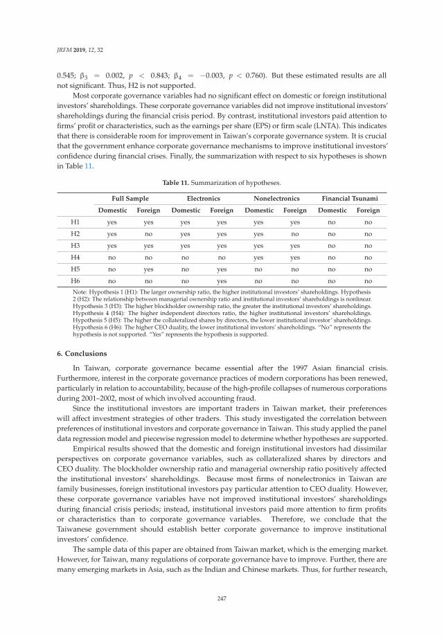
JRFM 2019, 12, 32
0.545; β3 = 0.002, p < 0.843; β4 = −0.003, p < 0.760). But these estimated results are allnot significant. Thus, H2 is not supported.
Most corporate governance variables had no significant effect on domestic or foreign institutionalinvestors’ shareholdings. These corporate governance variables did not improve institutional investors’shareholdings during the financial crisis period. By contrast, institutional investors paid attention tofirms’ profit or characteristics, such as the earnings per share (EPS) or firm scale (LNTA). This indicatesthat there is considerable room for improvement in Taiwan’s corporate governance system. It is crucialthat the government enhance corporate governance mechanisms to improve institutional investors’confidence during financial crises. Finally, the summarization with respect to six hypotheses is shownin Table 11.
Table 11. Summarization of hypotheses.
Full Sample Electronics Nonelectronics Financial Tsunami
Domestic Foreign Domestic Foreign Domestic Foreign Domestic Foreign
H1 yes yes yes yes yes yes no no
H2 yes no yes yes yes no no no
H3 yes yes yes yes yes yes no no
H4 no no no no yes yes no no
H5 no yes no yes no no no no
H6 no no no yes no no no no
Note: Hypothesis 1 (H1): The larger ownership ratio, the higher institutional investors’ shareholdings. Hypothesis2 (H2): The relationship between managerial ownership ratio and institutional investors’ shareholdings is nonlinear.Hypothesis 3 (H3): The higher blockholder ownership ratio, the greater the institutional investors’ shareholdings.Hypothesis 4 (H4): The higher independent directors ratio, the higher institutional investors’ shareholdings.Hypothesis 5 (H5): The higher the collateralized shares by directors, the lower institutional investor’ shareholdings.Hypothesis 6 (H6): The higher CEO duality, the lower institutional investors’ shareholdings. “No” represents thehypothesis is not supported. “Yes” represents the hypothesis is supported.
6. Conclusions
In Taiwan, corporate governance became essential after the 1997 Asian financial crisis.Furthermore, interest in the corporate governance practices of modern corporations has been renewed,particularly in relation to accountability, because of the high-profile collapses of numerous corporationsduring 2001–2002, most of which involved accounting fraud.
Since the institutional investors are important traders in Taiwan market, their preferenceswill affect investment strategies of other traders. This study investigated the correlation betweenpreferences of institutional investors and corporate governance in Taiwan. This study applied the paneldata regression model and piecewise regression model to determine whether hypotheses are supported.
Empirical results showed that the domestic and foreign institutional investors had dissimilarperspectives on corporate governance variables, such as collateralized shares by directors andCEO duality. The blockholder ownership ratio and managerial ownership ratio positively affectedthe institutional investors’ shareholdings. Because most firms of nonelectronics in Taiwan arefamily businesses, foreign institutional investors pay particular attention to CEO duality. However,these corporate governance variables have not improved institutional investors’ shareholdingsduring financial crisis periods; instead, institutional investors paid more attention to firm profitsor characteristics than to corporate governance variables. Therefore, we conclude that theTaiwanese government should establish better corporate governance to improve institutionalinvestors’ confidence.
The sample data of this paper are obtained from Taiwan market, which is the emerging market.However, for Taiwan, many regulations of corporate governance have to improve. Further, there aremany emerging markets in Asia, such as the Indian and Chinese markets. Thus, for further research,
247

JRFM 2019, 12, 32
the methodology and issues can be employed to analyze and compare effects of corporate governanceon institutional investors’ preferences among other emerging markets.
Author Contributions: S.-L.L. was the author behind the main idea and objectives of the paper. Y.-H.L. collectedand analyzed the data. S.-L.L. and Y.-H.L. drafted the manuscript. S.-L.L. completed further econometricestimations and revised the paper.
Funding: This research received no external funding.
Acknowledgments: We are grateful to the three anonymous referees for their helpful comments and suggestions.
Conflicts of Interest: The authors declare no conflict of interest.
References
Aggarwal, Reena, Leora Klapper, and Peter Wysocki. 2005. Portfolio Preferences of Foreign Institutional Investors.Journal of Banking and Finance 29: 2919–46. [CrossRef]
Appel, Ian, Todd Gormley, and Donald Keim. 2016. Passive investors, not passive owners. Journal of FinancialEconomics 121: 111–41. [CrossRef]
Beasley, Mark. 1996. An Empirical Analysis of the Relation between the Board of Director Composition andFinancial Statement Fraud. The Accounting Review 71: 443–65.
Bebchuk, Lucian, Alma Cohen, and Scott Hirst. 2017. The Agency Problems of Institutional Investors. DiscussionPaper. Cambridge: Harvard Law School.
Boyd, Brian. 1995. CEO duality and firm performance: A contingency model. Strategic Management Journal 16:301–12. [CrossRef]
Cadbury, Adrian. 1992. The Financial Aspects of Corporate Governance (Cadbury Report). London: The Committee onthe Financial Aspect of Corporate Governance (The Cadbury Committee) and Gee and Co., Ltd.
Carleton, Willard, James Nelson, and Michael Weisbach. 1998. The influence of institutions on corporategovernance through private negotiations: Evidence from TIAA-CREF. Journal of Finance 53: 1335–1362.[CrossRef]
Cao, Tingqui, Xiuli Yang, and Yuguang Sun. 2007. Ownership structure and corporate performance: Measurementmethod and endogeneity. Economic Research Journal 10: 126–37.
Chen, Ming-Yuan. 2006. Managerial ownership and firm performance: An analysis using switchingsimultaneous-equation models. Applied Economics 38: 161–81. [CrossRef]
Chiou, Jeng-Ren, Ta-Chung Hsiung, and Lanfeng Kao. 2002. A Study of the Relationship between FinancialDistress and Collateralized Shares. Taiwan Accounting Review 3: 79–111.
Choe, Hyuk, Bong-Chan Kho, and René M. Stluz. 1999. Do Foreign Investors Destabilize Stock Market? TheKorean Experience in 1997. Journal of Financial Economics 54: 227–64. [CrossRef]
Dahya, Jay, Laura Galguera Garcia, and Jos van Bommel. 2009. One Man Two Hats: What’s All Commotion!Financial Review 44: 179–212. [CrossRef]
Daily, Catherine, and Dane Dalton. 1993. Boards of directors, leadership and structure: Control and performanceimplications. Entrepreneurship Theory and Practice 17: 65–81. [CrossRef]
Dahlquist, Magus, and Gorän Robertsson. 2001. Direct Foreign Ownership, Institutional Investors, and FirmCharacteristics. Journal of Financial Economics 59: 413–440. [CrossRef]
Davies, J.R., David Hillier, and Patrick McColgan. 2005. Ownership structure, managerial behavior and corporatevalue. Journal of Corporate Finance 11: 645–60. [CrossRef]
De Miguel, Alberto, Julio Pindado, and Chabela de la Torre. 2004. Ownership structure and firm value: Newevidence from Spain. Strategic Management Journal 25: 1199–207. [CrossRef]
Driffield, Nigel, Vidya Mahambare, and Sarmistha Pal. 2007. How does ownership structure affect capitalstructure and firm value? Recent evidence from East Asia. Economics of Transition 15: 535–73. [CrossRef]
Dahya, Jay, Alasdair Lonie, and David Power. 1996. The case for separating the roles of chairman and CEO:An anaylsis of stockmarket and accounting data. Corporate Governance: An International Review 4: 71–77.[CrossRef]
Dahya, Jay, and Nickolaos Travlos. 2000. Does the one man show pay? Theory and evidence on the dual CEOrevisited. European Financial Management 16: 85–98. [CrossRef]
248

JRFM 2019, 12, 32
Faccio, Mara, and Meziane Lasfer. 1999. Managerial Ownership, Board Structure and Firm Value: The UKEvidence, Working Paper. Available online: https://papers.ssrn.com/sol3/papers.cfm?abstract_id=179008(accessed on 31 December 2018).
Fama, Eugene, and Michael Jensen. 1983. Separation of Ownership and Control. Journal of Law and Economics 26:301–25. [CrossRef]
Falkenstein, Eric. 1996. Preference for Stock Characteristics as Revealed by Mutual Fund Portfolio Holdings.Journal of Finance 51: 111–35. [CrossRef]
Florackis, Chrisostomos. 2005. Internal corporate governance mechanisms and corporate performance: Evidencefor UK firms. Applied Financial Economics Letters 1: 211–16. [CrossRef]
Florackis, Chrisostomos, Alexandros Kostakis, and Aydin Ozkan. 2009. Managerial ownership and performance.Journal of Business Research 62: 1350–57. [CrossRef]
Gompers, Paul, and Andrew Metrick. 2001. Institutional Investors and Equity Prices. Quarterly Journal of Economics116: 229–59. [CrossRef]
Griffith, John. 1999. CEO ownership and firm value. Managerial and Decision Economics 20: 1–8. [CrossRef]Hermalin, Benjamin, and Michael Weisbach. 1991. The effects of board composition and direct incentives on firm
performance. Financial Management 20: 101–12. [CrossRef]Holderness, Clifford, Randall Kroszner, and Dennis Sheehan. 1999. Were the good old days that good? Changes
in managerial stock ownership since the Great Depression. Journal of Finance 54: 435–470. [CrossRef]Huson, Mark, Robert Parrino, and Laura Starks. 2001. Internal Monitoring Mechanisms and CEO Turnover: A
Long-Term Perspective. Journal of Finance 56: 2265–97. [CrossRef]Jensen, Michael, and Willian Meckling. 1976. Theory of the Firm: Managerial Behavior, Agency Cost and
Ownership Structure. Journal of Financial Economics 3: 305–60. [CrossRef]Jensen, Michael. 1993. The Modern Industrial Revolution, Exit, and the Failure of Internal Control Systems. Journal
of Finance 48: 831–80. [CrossRef]Kao, Lanfeng, Jeng-Ren Chiou, and Anlin Chen. 2004. The Agency Problem, Firm Performance and Monitoring
Mechanisms: The Evidence from Collateralized Shares in Taiwan. Corporate Governance: An InternationalReview 12: 389–402. [CrossRef]
Keasey, Kevin, Helen Short, and Robert Watson. 1994. Directors’ ownership and the performance of small andmedium sized firms in the UK. Small Business Economics 6: 225–36. [CrossRef]
La Porta, Rafael, Florencio Lopez-de-Silanes, Andrei Shleifer, and Robert Vishny. 1997. Legal determinants ofexternal finance. Journal of Finance 52: 1131–50. [CrossRef]
La Porta, Rafel, Florencio Lopez-de-Silanes, Andrei Shleifer, and Robert Vishny. 1998. Law and finance. Journal ofPolitical Economy 106: 1115–55. [CrossRef]
La Porta, Rafel, Florencio Lopez-de-Silanes, Andrei Shleifer, and Robert Vishny. 2000. Investor protection andcorporate governance. Journal of Financial Economics 58: 3–27. [CrossRef]
Leuz, Christian, Dhananjay Nanda, and Peter Wysocki. 2003. Investor protection and earnings management: Aninternational comparison. Journal of Financial Economics 69: 505–27. [CrossRef]
Li, Lingfeng. 2002. Macroeconomic Factors and the Correlation of Stock and Bond Returns. International Centerfor Finance Yale University Working paper, November, No. 02-46. Available online: http://www.scielo.org.co/scielo.php?script=sci_nlinks&ref=000129&pid=S0121-5051201100010001200033&lng=en (accessed on 31December 2018).
McConnell, John, and Henri Servaes. 1990. Additional evidence on equity ownership and corporate value. Journalof Financial Economics 27: 595–612. [CrossRef]
McCahery, Joseph, Zacharias Sautner, and Laura T. Starks. 2016. Behind the scenes: The corporate governancepreferences of institutional investors. Journal of Finance 71: 2905–32. [CrossRef]
Morck, Randall, Andrei Shleifer, and Robert Vishny. 1988. Management Ownership and Market Evaluation: AnEmpirical Analysis. Journal of Financial Economics 20: 293–315. [CrossRef]
Mudambi, Ram, and Carmeia Nicosia. 1998. Ownership structure and firm performance: Evidence from the UKfinancial service industry. Applied Financial Economics 8: 175–80. [CrossRef]
Mura, Roberto. 2007. Firm performance: Do non-executive directors have a mind of their own? Evidence fromUK panel data. Financial Management 36: 81–112. [CrossRef]
Ng, Lilian, and Qinghai Wang. 2004. Institutional trading and the turn-of-the -year effect. Journal of FinancialEconomics 74: 343–66. [CrossRef]
249

JRFM 2019, 12, 32
Patton, Arch, and John Baker. 1987. Why won’t directors rock the board? Harvard Business Review 65: 10–18.Pi, Lynn, and Stephen Timme. 1993. Corporate control and bank efficiency. Journal of Banking and Finance 17:
515–30. [CrossRef]Prowse, Stephen. 1993. The structure of corporate ownership in Japan. The Journal of Finance 47: 1121–40.
[CrossRef]Rosenstein, Stuart, and Jeffrey Wyatt. 1997. Inside Directors, Board Effectiveness, and Shareholder Wealth. Journal
of Financial Economics 44: 229–50. [CrossRef]Shan, Neeta, and Christopher Napier. 2014. The Cadbury Report 1992: Shared Vision and Beyond; Essay. Egham:
Royal Holloway University of London. Available online: http://wwwdata.unibg.it/dati/corsi/900002/79548-Beyond%20Cadbury%20Report%20Napier%20paper.pdf (accessed on 31 December 2018).
Shleifer, Andrei, and Robert Vishny. 1997. A survey of corporate. The Journal of Finance 52: 737–38. [CrossRef]Short, Helen, and Kevin Keasey. 1999. Managerial ownership and the performance of firms: Evidence from the
UK. Journal of Corporate Finance 5: 79–101. [CrossRef]Stoeberl, Phillip, and Bruce C. Sherony. 1985. Board Efficiency and Effectiveness. In Handbook for Corporate
Directors. Edited by Edward Mattar and Michael Ball. New York: McGraw-Hill, pp. 12.1–12.10.Minguez-Vera, Antonio, and Juan Francisco Martin-Ugedo. 2007. Does ownership structure affect value? A panel
data analysis for the Spanish market. International Review of Financial Analysis 16: 81–98. [CrossRef]Weisbach, Michael. 1988. Outside Directors and CEO Turnover. Journal of Financial Economics 20: 431–60. [CrossRef]Yeh, Yin-Hua, and Tsun-Siou Lee. 2002. Corporate Governance and Corporate Equity Investments: Evidence from
Taiwan. Paper presented at 9th Global Finance Conference, Beijing, China, May 27–29.Zhang, Yu-Ren, Tay-Chang Wang, and Chung-Fern Wu. 2009. Evidence on the association between mechanisms
of corporate governance and the portfolio held by foreign investors. Journal of Management & Systems 16:505–32.
© 2019 by the authors. Licensee MDPI, Basel, Switzerland. This article is an open accessarticle distributed under the terms and conditions of the Creative Commons Attribution(CC BY) license (http://creativecommons.org/licenses/by/4.0/).
250
Journal of
Risk and FinancialManagement
Article
The Impact of Exchange Rate Volatility on Exports inVietnam: A Bounds Testing Approach
Vinh Nguyen Thi Thuy * and Duong Trinh Thi Thuy
Foreign Trade University, Hanoi 100000, Vietnam; [email protected]* Correspondence: [email protected]; Tel.: +84-24-3775-1278 (ext. 112)
Received: 15 November 2018; Accepted: 27 December 2018; Published: 4 January 2019
Abstract: This paper investigates the impact of exchange rate volatility on exports in Vietnam usingquarterly data from the first quarter of 2000 to the fourth quarter of 2014. The paper applies theautoregressive distributed lag (ARDL) bounds testing approach to the analysis of level relationshipsbetween effective exchange rate volatility and exports. Using the demand function of exports,the paper also considers the effect of depreciation and foreign income on exports of Vietnam.The results show that exchange rate volatility negatively affects the export volume in the longrun, as expected. A depreciation of the domestic currency affects exports negatively in the short run,but positively in the long run, consistent with the J curve effect. Surprisingly, an increase in the realincome of a foreign country actually decreases Vietnamese export volume. These findings suggestsome policy implications in managing the exchange rate system and promoting exports of Vietnam.
Keywords: exchange rate; volatility; exports; ARDL; Vietnam
1. Introduction
In 2015, the exchange rate became a hot issue for Vietnam’s economy with regard to concernsabout China’s devaluation of the Yuan, the increase of the federal fund rate of Fed, and the US dollarappreciation against many currencies in the world. Due to being pegged to the USD, the VietnamDong (VND) became more expensive against many foreign currencies, thus, the competitiveness ofVietnamese goods and the trade balance was affected negatively. The debatable policy question iswhether a dong-pegged-to-the-dollar policy over the years remains appropriate. From a corporateperspective, does the stability of the VND against USD support enterprises to avoid risk in internationalbusiness because the US dollar is the main payment currency, or enterprises may be adversely impactedby the uncertainty of bilateral exchange rates for currencies of different countries around the world?In the period of integrating into the world’s economy, Vietnam could be seriously challenged by theincrease in such risks, therefore, it is necessary to find a suitable exchange rate arrangement. Underthat situation, on 31 December 2015, the State Bank of Vietnam issued Decision No. 2730/QD-NHNNto announce the way to determine the central rate of the VND against the USD, which would be usedby financial institutions authorized to trade in foreign currencies. The rate is calculated based onthree benchmarks: demand and supply of the Vietnam Dong, the movement of eight currencies of thecountries having the largest weights for trading and investment with Vietnam, including the USD,the Euro, the Chinese Yuan, the Japanese Yen, the Singapore Dollar, the South Korean Won, the ThaiBaht, and the Taiwan Dollar, and macroeconomic balance.
However, whether the exchange rate stability based on the eight major currencies really bringsadvantages to international trade or not is still a significant question because of the mixed results oftheoretical, as well as empirical, studies on the impact of exchange rate volatility on international trade,although many studies also propose that mitigating exchange rate risk is very important to ensuringthat the exports of a country achieve sustained stable growth. Moreover, in Vietnam, economists often
JRFM 2019, 12, 6; doi:10.3390/jrfm12010006 www.mdpi.com/journal/jrfm251
JRFM 2019, 12, 6
study the impact of exchange rate movement on the trade balance, inflation, and economic growth,while studies concentrating on measuring and assessing the influence of exchange rate volatility arestill limited, especially in regards to the macro approach. Therefore, it is worthwhile to investigate theeffect of exchange rate volatility on exports in the Vietnam context.
For all of the above reasons, this paper investigates the impact of exchange rate volatility betweenVND and the basket of eight foreign currencies referred to in the central rate benchmark on exportsof the Vietnamese economy using quarterly data from the first quarter of 2000 to the fourth quarterof 2014 and the Autoregressive Distributed Lag (ARDL) method of Pesaran et al. (2001). Pesaran’sARDL method shows having comparatively superior forecasting performance compared to the othertechniques based on co-integration (Iqbal and Uddin 2013; Adom and Bekoe 2012). The result showsthat export performance will be impacted by exchange rate volatility in the long run. A one percentincrease in exchange rate volatility will reduce export volume significantly by about 0.11 percent.However, an appreciation of the domestic currency can adversely affect the competitiveness ofVietnamese exports in the international market in the short run, while the Vietnam Dong’s devaluationwill have positive impacts and improve exports in the long run. A surprising finding is that realforeign income has a negative impact on export volume of Vietnam in both the long run and theshort run. The findings provide some implications for managers, policymakers, and entrepreneurs.The remainder of the paper is organized as follows: Section 2 reviews the theoretical background andeconometric techniques for examining the effect of exchange rate volatility on exports. Next, Section 3describes the model, methodology and relevant data used for quantitative assessment in the case ofVietnam. Then, the estimation results are discussed in Section 4. Finally, Section 5 concludes with asummary of findings and policy recommendations.
2. Theoretical Framework and Literature Review
Different theories exist in the literature regarding the impact of exchange rate volatility on exporterbehavior. An increase in exchange rate volatility may be associated with either an increase or a decreasein the volume of exports, given plausible alternative assumptions.
Traditionally, it has been argued that exchange rate volatility will have a negative influenceon exports. Clark (1973) analyses a very early example, in which a firm produces a homogenouscommodity and exports its products entirely to one foreign market. In this basic model, the market isconsidered as perfectly competitive and imported inputs are not required. The firm receives paymentsfor its exports in foreign currency and hedging possibilities are extremely limited. Owing to adjustmentcosts, the firm cannot change its output over the planning horizon. The unpredictable variation of theexchange rate, therefore, is solely blame for uncertainty about future export sales as well as futureprofits in domestic currency. For the sake of maximizing the expected value of utility, which dependson both the expected value and the variance of profits, the risk-averse firm would reduce its exposure torisk in response to higher volatility in the exchange rate. That is, the volume of production, and henceexports would be cut down in this circumstance. This simple model is also developed by a number ofauthors, for example, Baron (1976b); Hooper and Kohlhagen (1978), indicated the same conclusionthat exchange rate volatility has a negative effect on exports.
However, all of those conclusions result from several restrictive assumptions. One obviouscriticism of the traditional models is that the exporter’s risk exposure is attributed solely to the exchangerate volatility, whereas it may depend on the availability of hedging techniques, diversificationpossibilities, the existence of imported inputs, and other factors. The rationale of this assumption is thatforward exchange markets are just in infancy or even not appear in developing economies. In addition,transaction hedging may prove relatively expensive and challenging for some manufacturing firmswith a long time between order and delivery. However, this is not the case with advanced countries,in which such markets are well-developed. For risk-adverse entrepreneurs who can hedge theircontracts, a higher exchange rate volatility would not always deter exports, as noted by Ethier (1973)and Baron (1976a). Furthermore, the companies can minimize exchange rate risk in other ways; take
252

JRFM 2019, 12, 6
multinational cooperation to be a good case in point. Being involved in a wide range of trade andfinancial transactions over numerous countries, it would see an abundance of diverse opportunitiesto offset the movement of a bilateral exchange rate, such as the variability of other exchange rates orinterest rates. Relaxing the assumption of no imported intermediate inputs, Clark (1973) finds that theloss from the depreciation in a foreign currency to the exporter will be partly alleviated by loweringinput cost. Likewise, if inventories are possible and firms can allocate their sales between abroadand home markets, a declining effect on export earnings will also be compensated. More generally,from a finance perspective, Makin (1978) argues that a diversified firm holding a portfolio of assetsand liabilities determined in various currencies will be able to protect itself from exchange rate risksrelated to exports and imports. Finally, recent studies suggest that exchange rate volatility does notjust embody a risk, but profit opportunities. For instance, as examined by Canzoneri et al. (1984), if afirm has ability to alter its factor inputs to benefit from changes in exchange rate without adjustmentcosts, a higher volatility may create greater probability to make profit. Gros (1987) derives a furtherversion of model with the presence of adjustment costs, in which exporting can be seen as an optiondepending on capacity, taking advantage of favorable conditions (e.g., high prices) and to minimizingthe influence otherwise. The value of the option rises as result of higher variability of the exchangerate, creating a positive effect on exports. Therefore, the effect of volatility remains ambiguous becausethe dominant direction depends on a case-by-case basis.
In the early models, the negative association between exchange rate volatility and expected exportincreases is supported in terms of risk aversion. The uncertainty of the exchange rate seems to notaffect a risk-neutral firm’s decision. Nonetheless, De Grauwe (1988) argues that the assumption ofrisk-averse agents is not adequate to ensure the direction of this link. What is relevant is the degree ofrisk aversion. An increase in risk, in general, has both a substitution and an income effect that work inopposite directions (Goldstein and Khan 1985). The substitution effect discourages risk-averse agentsto export because it lowers the expected utility representing the attractiveness of the risky activity,while the income effects urges very risk-averse agents to increase their exports to avoid the possibilityof a severe decline in the revenues. Taken together, these studies support the notion that even thoughfirms are worse off with an increase in exchange rate risk, their response may be to export more ratherthan less.
All of the theoretical studies reviewed here support the notion that the net effect of exchange ratevolatility on exports is ambiguous, as differing results can arise from plausible alternative assumptionsand modelling strategies. Increased exchange rate volatility can have no significant effect on exports,or where significant, no systematic effect in one direction or the other.
Numerous empirical studies have been conducted in many countries and areas around the worldto evaluate the impact of exchange rate volatility on exports. Again, the implications of the resultsof those studies confirm that, although exchange rate volatility has an impact on exports, the effectcan be either positive or negative depending on the endowment of each country; whether empiricalstudies use aggregate data, sectoral data or bilateral data; and the econometric techniques applied.
The empirical literature using aggregate data tends to find weak evidence in favor of a negativeimpact of exchange rate uncertainty on the trade flows of a country to the rest of the world. Using theEngel-Granger method, Doroodian (1999) approximated volatility with both Autoregressive IntegratedMoving Average (ARIMA) and Generalized Autoregressive Conditional Heteroskedasticity (GARCH)techniques to study the exports of India, Malaysia, and South Korea from the second quarter of 1973 tothe third quarter of 1996. The results reveal significantly negative effects of exchange rate volatility onexports. Meanwhile, employing the Johansen approach of co-integration and using AutoregressiveConditional Heteroskedasticity (ARCH) method to calculate volatility, Arize and Malindretos (1998)found mixed results for two Pacific-Basin countries: volatility is shown to depress New Zealandexports, while its impact is positive in the case of Australia.
To sum up, the majority of empirical studies indicate that the relationship between a singlecountry’s exports and exchange rate volatility is statistically significantly negative in the long run,
253

JRFM 2019, 12, 6
especially in developing countries, while others consider that there is the positive relationshipin the short run or long run. The basis for empirical model development is mostly based onsimple demand functions of exports. Relative prices, income, and volatility are often employedas determinants. There are two major problems facing the applied econometrics in these studies.Firstly, there has not yet been a standard exchange rate volatility proxy (Bahmani-Oskooee andHegerty 2007). Some measure of variance has dominated this field, but the precise calculation of thismeasure differs from study to study. Later estimates have involved using the standard deviation ofa rate of change or the level of a variable. Kenen and Rodrik (1986) draw attention to the movingstandard deviation of the monthly change in the exchange rate, which has the advantage of beingstationary. Utilizing newer time-series methods, Engle and Granger (1987) developed AutoregressiveConditional Heteroskedasticity (ARCH) as a measure of volatility in time-series errors, which is awidespread measure of exchange rate volatility in the literature. A broader perspective is adopted by(Pattichis 2003) who develops Generalized Autoregressive Conditional Heteroskedasticity (GARCH),which incorporates moving-average processes. These authors’ estimates also have the desirableproperty of stationarity. Some measures are more popular than others, however, none stands outas the standard volatility proxy (Bahmani-Oskooee and Hegerty 2007). The second problem is thetype of method used in estimating the empirical model. While the Ordinary Least Squares (OLS) wascommonly used in the early papers, newer and more sophisticated techniques, including time-seriesand panel data methods, in recent studies have facilitated investigation of the sensitivity of exportsto a measure of exchange rate volatility. The main goal of modern time-series analysis is to take intoconsideration integrating properties of the variables so that spurious results can be avoided. Somepopular methods of time-series analysis in recent years are the Engle-Granger method, the Johansenmethod, and the bounds testing approach.
3. Exchange Rate Volatility Measurement
Exchange rate volatility denotes the amount of uncertainty or risk about the size of changes inthe exchange rate. If the exchange rate can potentially be spread out over a larger range of values in ashort time span, it is termed to have high volatility. If the exchange rate does not fluctuate dramatically,and tends to be steadier, it is termed to have low volatility. Additionally, real and nominal exchangerate volatilities are different for practical purposes. The properties of the method used to estimatevolatility have also received lots of attention. Bahmani-Oskooee and Hegerty (2007) emphasizes thefact that a clearly dominant approximation for uncertainty has not yet emerged up to now.
In this paper, the exchange rate volatility is measured by the moving average of the standarddeviation of exchange rates, which is typically used by a number of scholars such as Chowdhury (1993);Arize and Malindretos (1998); Kasman and Kasman (2005). This equation is as follows:
VOLt =
[1m
m
∑i=1
(ERt+i−1 − ERt+i−2)2
] 1m
(1)
where m is the number of periods; and t is time and ER refers to the exchange rate index. In our study,m = 2.
Bagella et al. (2006) show advantages of effective exchange rate volatility comparing with bilateralexchange rate volatility and find that this variable performs much better than the bilateral exchangerate volatility measure. An important advantage is that the effective exchange rate reflects moresufficiently the stability of a country which might have low bilateral exchange rate volatility witha leading currency but absorb instability via variability of economic policies of its trade partners.Therefore, we use the nominal effective exchange rate between the VND and a foreign currency basket(NEER) to compute the exchange rate volatility. This selected basket consists of eight foreign currenciesused by the SBV to refer to the central exchange rate from the beginning of 2016, including: USD(United States), EUR (EU), CNY (China), THB (Thailand), JPY (Japan), SGD (Singapore) KRW (Korea),
254

JRFM 2019, 12, 6
and TWD (Taiwan). This option aims to assess the validity of the new exchange rate policy for exportpurposes. Following the splicing procedure proposed by Ellis (2001), this index is computed as:
NEERt = NEERt−1∏8
j=1
(NERj
t
)ωjt
∏8j=1
(NERj
t−1
)ωjt(2)
where NEERt is the real effective exchange rate of Vietnam at time t; NERjt is the nominal bilateral
exchange rate relative to currency of country j, measured as the number of units of the domesticcurrency per unit of currency of country j and expressed as an index; ωjt is the weight assigned to thecurrency of country j at time t, reflecting the contribution of the country j to Vietnam’s foreign trade,∑8
j=1 ωjt = 1.In Equation (2), the nominal effective exchange rate is calculated as the ratio of geometrically
weighted bilateral nominal exchange rates in the current period and in the preceding period, usingcurrent weights, spliced onto the preceding level of nominal effective exchange rate. There are twomain advantages associated with the use of this approach. Firstly, the weights are allowed to vary overtime in order to account for the possibility that some countries may become more important tradingpartners. Otherwise, if actual trade shares move significantly and this is not taken into consideration,the effective exchange rate would give a misleading picture of the net effect of movements in particularbilateral exchange rates. Secondly, as changing weights are updated, it is important that the exchangerate index should be spliced together with the previous observation. Otherwise, in periods in which theweights change, it would not be clear whether a change in the NEER is reflecting changes in the weights
or in the bilateral exchange rates, as we can see from a common calculation: NEERt = ∏8j=1 (NERj
t)wjt
.There are some prior studies using this approach, such as Moccero and Winograd (2006); Chinn (2006);Betliy (2002); Dullien (2005).
Data for bilateral exchange rates and trade weights are computed from International FinancialStatistics (IFS) and Direction of Trade Statistics (DOTS) of IMF.
Figure 1 describes the volatility of NEER of the Vietnam Dong versus the eight currency basketfor the period from the first quarter of 2000 to the fourth quarter of 2014. The degree of this volatilitydepends on the exchange rate policy and the fluctuation of foreign currencies in the world market.As can be seen from Figure 1, the NEER volatility fluctuated gradually from 2000 to 2007, dramaticallyincreased during the following four years and decreased between 2012 and 2014.
0
2
4
6
8
10
12
VOL
Figure 1. Vietnamese NEER volatility (2000 Q1–2014 Q4).
After introducing a new principle for setting the exchange rate in 1999, the volatility from 2000 to2008 was relatively small as the official exchange rate was almost unchanged. During the period from2008 to 2011, the State Bank of Vietnam had devalued three times the Vietnam Dong by approximately
255
JRFM 2019, 12, 6
10% and adjusted the trading band in commercial banks continuously (widened the band five timesfrom ±0.5% to ±5% and then narrowed it back to 1%). These actions increased the exchange ratefluctuation. From 2012 to 2014, the official exchange rate remained stable except for a devaluation inJune 2013 and the trading band was fixed at ±1%, therefore, the volatility was small.
4. Empirical Investigation
4.1. Econometric Model
According to the microeconomic theory, conventional demand functions are homogenous degreezero in terms of price and income (Deaton and Muellbauer 1980). To examine the impact of exchangerate volatility on exports, this study adds an exchange rate volatility variable to the traditionalexport demand function comprising consumers’ income (or GDP) and relative price, which has beenused in many previous studies such as Salas (1982); Gafar (1995); Matsubayashi and Hamori (2003);Ekanayake et al. (2010). The model is specified as follows:
Xt = β0 + β1GDP_Ft + β2REERt + β3VOLt + εt (3)
where X represents real exports; GDP_F is real foreign income; REER is the real effective exchangerate; and VOL is the exchange rate volatility. With regard to the functional form, Khan and Ross (1977)suggest that a log-linear specification is better than a standard linear one on both empirical andtheoretical grounds. That is, the former allows the dependent variable to react proportionally toan increase or decrease in the regressors and exhibits interaction between elasticities. Therefore, allvariables in Equation (3) are expressed in logarithmic form. In Equation (3) we have the followingexpectations for the sign of the regression coefficients: According to the gravity theory of internationaltrade, increases in real GDP of trading partners would be expected to result in greater real exportsto those partners, therefore, β1 > 0. Due to the relative price effect, the real exchange rate may leadto an increase in the volume of export, therefore, β2 > 0. The relationship between the exchange ratevolatility and export volume is ambiguous, thus, it is expected that β3 > 0 or β3 < 0.
When modelling the relationship between a set of time-series variables, it is important to takeinto account the stationarity of the data. When detecting a spurious regression problem amongthese series including a unit root, some methods are suggested to solve this problem. One of thesimplest ways is taking the differences of the series and estimating a standard regression model.However, this method results in the loss of information that is meaningful for the level relationships.Provided that the first differences of the variables are used, it is impossible to determine a potentiallong run relationship in levels. Moving from this point, the co-integration approach associated witherror-correction modelling was developed during the late 1980s. In this way, both the short runand long run relationship can be analyzed. The co-integration approach developed by Engle andGranger (1987) is suitable for the test based on the expectation of only one co-integrating vectorbeing present. Further, the approach proposed by Johansen (1988) enables researchers to test the casethat there is more than one co-integration vector by using the VAR model in which all the variablesare accepted as endogenous. However, the important condition that must be met to perform thesestandard co-integration tests is that all series should not be stationary at levels and they should beintegrated of the same order. In order to overcome this problem, Pesaran et al. (2001) have developedthe bounds test approach. According to this method, the existence of a co-integration relationshipcan be investigated between the time-series regardless of whether they are I(0) or I(1) (under thecircumstance that the dependent variable is I(1)). This point is the greatest merit of the bounds testover conventional co-integration testing. Moreover, this approach can distinguish dependent andindependent variables and is more suitable than another method for dealing with small sample sizes(Ghorbani and Motallebi 2009). In addition, different variables can be assigned different lag lengths asthey enter the model.
256
JRFM 2019, 12, 6
As reviewed by Bahmani-Oskooee and Hegerty (2007), while common variables in trade modelsare non-stationary series, most measures of exchange rate volatility are stationary. Therefore, theARDL approach by Pesaran et al. (2001) is the most highly recommended to investigate the effectof exchange rate volatility on exports. There are some prior studies using this approach, such asDe Vita and Abbott (2004); Sekantsi (2008); Yin and Hamori (2011); and Alam and Ahmad (2011).To implement the bounds test procedure, Equation (3) is modelled as a conditional ARDL errorcorrection model as follows:
LEXt = α0 + β0t +l1
∑i=1
δ1iLEXt−i
l2
∑i=1
δ2iLGDP_Ft−i
l3
∑i=1
δ3iLREERt−i
l4
∑i=1
δ4iLVOLt−i + ut (4)
ΔLEXt = α1 + γ0t + θ1LEXt−1 + θ2LGDPFt−1 + θ3LREERt−1 + θ4LVOLt−1
+l1−1∑
i=1λ1iΔLEXt−i +
l2−1∑
i=1λ2iΔLGDP_Ft−i +
l3−1∑
i=1λ3iΔLREERt−i +
l4−1∑
i=1λ4iΔLVOLt−i + ut
(5)
where LEX, LGDP_F, and LREER are the natural logarithms of real exports, real foreign income, and thereal effective exchange rate (all data are seasonally adjusted); LVOL is the natural logarithm of thenominal exchange rate volatility of Vietnam; l1, l2, l3, l4 are lag-lengths; θ1, θ2, θ3, θ4 are long-runcoefficients; and λ1i, λ2i, λ3i, λ4i are short-run coefficients (if the co-integration vector exists) and ut isa random disturbance term.
According to Pesaran et al. (2001), the ARDL approach uses two main steps to estimate the levelrelationship. The first step is the co-integration test to determine whether a level relationship existsbetween the variables in Equation (4). The null hypothesis of no level relationship among variables istested. This test is performed on the basis of comparing the computed F-statistic values with boundson critical values which depend on the number of variables. Furthermore, some later studies proposethe critical value table for special cases, such as the study by Narayan (2005) dealing with small samplesize. For various situations, those authors give lower and upper bounds on the critical values. In eachcase, the lower bound is based on the assumption that all the variables are I(0), and the upper bound isbased on the assumption that all the variables are I(1). If the estimated F-statistic falls below the lowerbound we cannot reject the null hypothesis, so no co-integration is possible. If the F-statistic exceedsthe upper bound, we conclude that we have co-integration. Finally, if the F-statistic falls betweenthe bounds, the test is inconclusive. If the long-run relationship is established between the variables,the long-run and short-run coefficients can be obtained by using the ARDL approach. The appropriatelag orders of variables are chosen using the Schwarz Information Criterion (SIC).
4.2. Data and Data Sources
The study uses quarterly data from the first quarter of 2000 to the fourth quarter of 2014, including60 observations. This period is used for research in order to minimize the problems associated withmonetary policy changes. Data for real exports (EX) is collected from the General Statistics Officeof Vietnam (GSO). Real foreign income (GDP_F) is measured by the export weighted GDP VolumeIndex of the twenty largest export partners during this period (United States, Japan, China, Australia,Singapore, Germany, Korea, Malaysia, United Kingdom, Philippines, Netherlands, Thailand, Canada,France, Indonesia, Switzerland, Belgium, Hong Kong, Italy, and Spain). GDP_F is calculated as follows:
GDP_Ft =20
∏j=1
(Yjt)ϕjt (6)
where Yjt is the real GDP of each partner, calculated by the GDP Volume Index, collected from the IFSdataset; ϕjt is the export weight assign to partner j at time t, computed by using data from the DOTSand ∑20
j=1 ϕjt = 1.
257
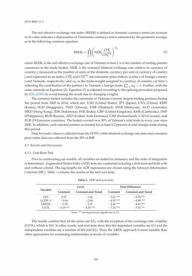
JRFM 2019, 12, 6
The real effective exchange rate index (REER) is defined in domestic currency terms (an increasein its value indicates a depreciation of Vietnamese currency) and is estimated by the geometric average,as in the following common equation:
REERt =n
∏j=1
(NERj
tCPIj
t
CPIVNt
)wjt
(7)
where REERt is the real effective exchange rate of Vietnam at time t; n is the number of trading-partnercurrencies in the trade basket; NERj
t is the nominal bilateral exchange rate relative to currency ofcountry j, measured as the number of units of the domestic currency per unit of currency of countryj and expressed as an index; CPIj
t and CPIVNt are consumer price indices at time t of foreign country
j and Vietnam, respectively; and ωjt is the trade-weight assigned to currency of country j at time t,reflecting the contribution of the partner j to Vietnam’s foreign trade, ∑n
j=1 ωjt = 1. Further, with thesame rationale as Equation (2), Equation (7) is adjusted according to the splicing procedure proposedby Ellis (2001) to avoid biasing the result due to changing weights.
The currency basket includes the currencies of Vietnam’s twenty largest trading partners duringthe period from 2000 to 2014, which are: USD (United States), JPY (Japan), CNY (China), KRW(Korea), SGD (Singapore), TWD (Taiwan), THB (Thailand), MYR (Malaysia), AUD (Australia),HKD (Hong Kong), IDR (Indonesia), INR (India), GBP (United Kingdom), KHR (Cambodia), PHP(Philippines), RUB (Russia), AED (United Arab Emirates), CHF (Switzerland), CAD (Canada), andEUR (19 Eurozone countries). The basket covered over 90% of Vietnam’s total trade in every year since2000. In addition, each selected partner accounted for at least 0.2 percent of total foreign trade duringthis period.
Data for trade values is collected from the DOTS, while bilateral exchange rate data and consumerprice index data are collected from the IFS of IMF.
4.3. Results and Discussions
4.3.1. Unit Root Test
Prior to constructing our models, all variables are tested for stationary and the order of integrationis determined. Augmented Dicker Fuller (ADF) tests are conducted including a drift term and both withand without a trend. The lag-lengths for ADF regressions are chosen using the Schwarz InformationCriterion (SIC). Table 1 contains the results of the unit root tests.
Table 1. ADF unit root tests.
VariableLevel First Difference
Constant Constant and Trend Constant Constant and Trend
LEX 0.37 −1.46 −9.61 *** −9.55 ***LGDP_F −0.64 −2.98 −4.92 *** −4.89 ***LREER −0.39 −2.37 −4.46 *** −4.61 ***LVOL −4.19 *** −4.30 *** −7.32 *** −7.32 ***
Note: *** are respectively significant at 1%.
The results confirm that all the series are I(1), with the exception of the exchange rate volatility(LVOL), which is I(0). In other words, unit root tests show that the dependent variables are I(1) and theindependent variables are a mixture of I(0) and I(1). Thus, the ARDL approach is more suitable thanother approaches for examining relationships in levels of variables.
258

JRFM 2019, 12, 6
4.3.2. Bounds Testing for Level Relationships
Using Schwarz (Bayes) criterion to find optimal lags, the EVIEWS 9.5 software developed by IHSMarkit (London, UK) suggests the model of ARDL (2,0,2,7).
A key assumption in the Bounds Testing methodology of Pesaran et al. (2001) is that the errors ofEquation (6) must be serially independent. This requirement may also be influential in the choice ofoptimal lags for the variables in the model. We use the LM test to test the null hypothesis of no serialcorrelation. The result indicates that at the 1% significance level, we cannot reject the null hypothesis,therefore, the selected model is suitable to test the cointegration relationship between the variables.
Due to the small sample size, we use the critical value bounds given by Narayan (2005). The resultof bounds testing is shown in Table 2.
Table 2. F-statistics to test the existence of long run relationships.
Model
Number ofRegressors
SampleSize
Estimated FTest Value
Critical Values Bounds-Narayan (2005),Unrestricted Intercept and Unrestricted Trend
k n F-Statistic10% 5% 1%
I(0) I(1) I(0) I(1) I(0) I(1)
ARDL(2,0,2,7)
3 52 14.576 3.673 4.715 4.368 5.545 5.995 7.335
As can be seen from the table, the calculated F-statistic of 14.576 exceeds the upper bounds, thissupports the existence of level relationships between real exports, real foreign income, real effectiveexchange rate and exchange rate volatility in the export equation. The selected ARDL model isrewritten as a single error correction model to identify long run and short run relationships.
4.3.3. Short run and Long run Relationship
By normalizing the exports, from the ARDL (2,0,2,7), the empirical results of the relationships inlevels are presented in Equation (8):
LEXt = 0.047t − 1.403LGDP_Ft + 0.987LREERt − 0.102LVOLt + et
(0.004) ∗ ∗ ∗ (0.344) ∗ ∗ ∗ (0.139) ∗ ∗ ∗ (0.012) ∗ ∗∗ (8)
Note: *** are respectively significant of 1%, the standard errors are in parenthesis.The estimation result suggests that all of variables could significantly explain the variation in
exports at the 1% level of significant.The estimated coefficient of VOL is about −0.11 percent, implying that the exchange rate volatility
has a negative impact on real exports. A one percent increase in the volatility reduces Vietnameseexports by about 0.11%. This is in line with the theoretical models of the behavior of risk adverseexporters in Clark (1973); Kohlhagen (1978), etc.; Arize and Malindretos (1998) argue that higherexchange rate volatility will depress export volume through a rise in adjustment costs like irreversibleinvestment due to higher uncertainty and risks.
At the macro level, this result is consistent with Qian and Varangis (1994) from consideringthe cases of developing countries. In these countries, the means of payment in international tradeis in foreign currency and the degree of dollarization is fairly high (always above 15 percent inVietnam), hence, the impact of exchange rate volatility is significant to economic activities. In addition,in developing countries like Vietnam, the derivative markets are underdeveloped, so that hedging maynot only be limited but also costly. Another possible explanation for the long run negative impact ofexchange rate volatility is that the higher the risk, the higher the value of options, leading to increasedcosts to ensure the future profit. This reduces the transaction volume in the market.
However, for the short run relationships shown in Table 3, all coefficients of the first difference ofVOL are positive and statistically significant at the 1% level, indicating that if exchange rate volatility
259
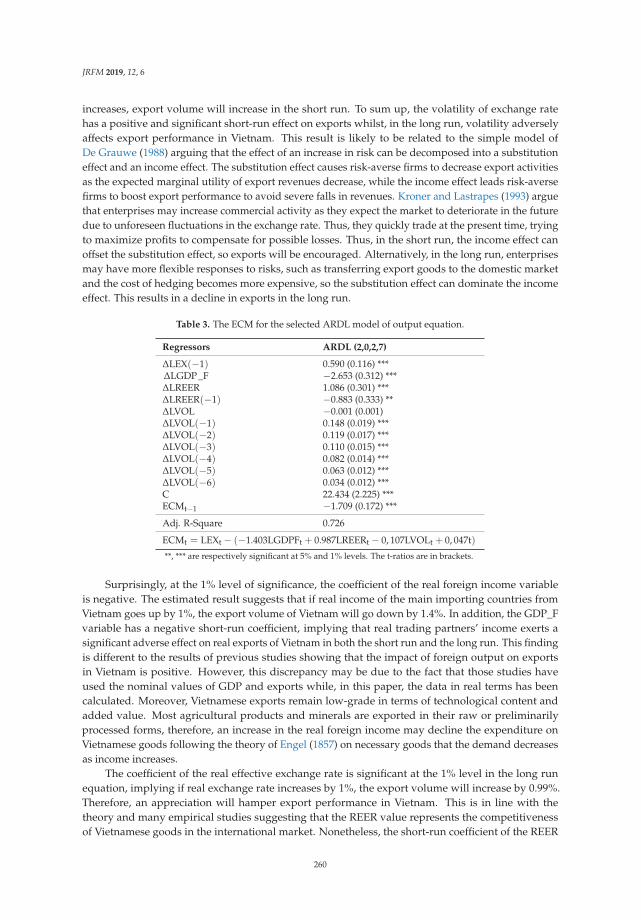
JRFM 2019, 12, 6
increases, export volume will increase in the short run. To sum up, the volatility of exchange ratehas a positive and significant short-run effect on exports whilst, in the long run, volatility adverselyaffects export performance in Vietnam. This result is likely to be related to the simple model ofDe Grauwe (1988) arguing that the effect of an increase in risk can be decomposed into a substitutioneffect and an income effect. The substitution effect causes risk-averse firms to decrease export activitiesas the expected marginal utility of export revenues decrease, while the income effect leads risk-aversefirms to boost export performance to avoid severe falls in revenues. Kroner and Lastrapes (1993) arguethat enterprises may increase commercial activity as they expect the market to deteriorate in the futuredue to unforeseen fluctuations in the exchange rate. Thus, they quickly trade at the present time, tryingto maximize profits to compensate for possible losses. Thus, in the short run, the income effect canoffset the substitution effect, so exports will be encouraged. Alternatively, in the long run, enterprisesmay have more flexible responses to risks, such as transferring export goods to the domestic marketand the cost of hedging becomes more expensive, so the substitution effect can dominate the incomeeffect. This results in a decline in exports in the long run.
Table 3. The ECM for the selected ARDL model of output equation.
Regressors ARDL (2,0,2,7)
ΔLEX(−1) 0.590 (0.116) ***ΔLGDP _F −2.653 (0.312) ***ΔLREER 1.086 (0.301) ***ΔLREER(−1) −0.883 (0.333) **ΔLVOL −0.001 (0.001)ΔLVOL(−1) 0.148 (0.019) ***ΔLVOL(−2) 0.119 (0.017) ***ΔLVOL(−3) 0.110 (0.015) ***ΔLVOL(−4) 0.082 (0.014) ***ΔLVOL(−5) 0.063 (0.012) ***ΔLVOL(−6) 0.034 (0.012) ***C 22.434 (2.225) ***ECMt−1 −1.709 (0.172) ***
Adj. R-Square 0.726
ECMt = LEXt − (−1.403LGDPFt + 0.987LREERt − 0, 107LVOLt + 0, 047t)
**, *** are respectively significant at 5% and 1% levels. The t-ratios are in brackets.
Surprisingly, at the 1% level of significance, the coefficient of the real foreign income variableis negative. The estimated result suggests that if real income of the main importing countries fromVietnam goes up by 1%, the export volume of Vietnam will go down by 1.4%. In addition, the GDP_Fvariable has a negative short-run coefficient, implying that real trading partners’ income exerts asignificant adverse effect on real exports of Vietnam in both the short run and the long run. This findingis different to the results of previous studies showing that the impact of foreign output on exportsin Vietnam is positive. However, this discrepancy may be due to the fact that those studies haveused the nominal values of GDP and exports while, in this paper, the data in real terms has beencalculated. Moreover, Vietnamese exports remain low-grade in terms of technological content andadded value. Most agricultural products and minerals are exported in their raw or preliminarilyprocessed forms, therefore, an increase in the real foreign income may decline the expenditure onVietnamese goods following the theory of Engel (1857) on necessary goods that the demand decreasesas income increases.
The coefficient of the real effective exchange rate is significant at the 1% level in the long runequation, implying if real exchange rate increases by 1%, the export volume will increase by 0.99%.Therefore, an appreciation will hamper export performance in Vietnam. This is in line with thetheory and many empirical studies suggesting that the REER value represents the competitivenessof Vietnamese goods in the international market. Nonetheless, the short-run coefficient of the REER
260

JRFM 2019, 12, 6
variable is negative and highly significant. Thus, a depreciation of the domestic currency affectsexports negatively in the short run, but positively in the long run, consistent with the J curve effect.
Table 3 provides the summary of the error correction representation of the estimated ARDL model.The empirical results indicate that the error correction term has the correct sign (negative) and isstatistically significant. This is further evidence of co-integration relationships among the variables inthe model. The estimated value of the error correction term implies that the speed of adjustment to thelong run equilibrium in response to the disequilibrium caused by short-run shocks of the previousperiod is 170.5% in the export equation.
4.3.4. Diagnostic Testing
The diagnostic tests including the normality test, serial correlation test, and heteroscedasticity testgenerally provide satisfactory outcomes.
Finally, the stability of the long-run coefficients along with the short run dynamics are evaluatedby applying the CUSUM and CUSUMSQ (Brown et al. 1975). The CUSUM test uses the cumulativesum of recursive residuals, whereas the CUSUMSQ test is based on the cumulative sum of the squaredrecursive residuals. As shown in Figure 2 both plots of CUSUM statistics and CUSUMSQ statisticsstay within the critical bounds of the 5% significance level (represented by the pair of straight linesdrawn at the 5% level of significance). These tests indicate no evidence of any significant structuralinstability. Therefore, the estimated results are stable over the studied time period.
(a)
(b)
-20
-15
-10
-5
0
5
10
15
20
2007 2008 2009 2010 2011 2012 2013 2014
CUSUM 5% Significance
-0.4
-0.2
0.0
0.2
0.4
0.6
0.8
1.0
1.2
1.4
2007 2008 2009 2010 2011 2012 2013 2014
CUSUM of Squares 5% Significance
Figure 2. Plot of cumulative sum of recursive residuals recursive residuals (a) and cumulative of squaresof recursive residuals (b). The straight lines represent critical bounds at the 5% significance level.
5. Conclusions
This paper aims to examine the impact of exchange rate volatility on Vietnamese exportsperformance during the period from the first quarter of 2000 to the fourth quarter of 2014. We usethe Moving Average of Standard Deviation (MASD) model and nominal effective exchange ratescomputed by a weighted average of the nominal bilateral exchange rate of the Vietnam Dong againstthe basket of eight foreign currencies to measure exchange rate volatility. This paper also applies anapproach called the Autoregressive Distributed Lag (ARDL) to investigate the existence of a levelrelationship among variables in the model and implements it using EVIEWS software offered by IHSMarkit (London, UK). The advantage of this approach is that it is suitable for small sample size andregressors which are a mixture of I(0) and I(1).
It is found that there exists a co-integration relationship between real exports, real foreign income,real effective exchange rate, and nominal exchange rate volatility. In addition, the speed of adjustmentto the long run equilibrium is fairly high.
261

JRFM 2019, 12, 6
The result shows that export performance will be impacted by exchange rate volatility in the longrun. A one percent increase in exchange rate volatility will reduce export volume significantly byabout 0.11 percent. One anticipated finding is that real foreign income has a negative impact on exportvolume of Vietnam in both the long run and the short run. As the income of trading partners increases,they tend to import fewer Vietnamese goods, which reflects that the position of Vietnamese goods inthe international market remains low-grade. Finally, an appreciation of the domestic currency canadversely affect the competitiveness of Vietnamese exports in the international market in the short run,while the Vietnam Dong’s devaluation will have positive impacts and improve exports in the long run.Since the inflation rate of Vietnam is unstable, it may impact the exporters’ expectations of movementof real exchange rate. We will deal with this issue for our future empirical research.
These findings have some important policy implications. Firstly, for the State Bank of Vietnam,the conversion of the exchange rate regime from announcing a solid exchange rate between the VNDand the US to announcing a central rate and cross rates with eight strong currencies is the rightdirection to promote export performance. The weighting for these currencies in the basket may becalculated based on stabilizing the nominal effective exchange rate with these eight currencies toreduce exchange rate uncertainty.
Secondly, besides considering exchange rate policy, it is essential for the government to adaptsynchronous implementation solutions to overcome the bottlenecks in Vietnamese exports. Productioncost, brand value, product quality, and technology content are key factors which threaten to decreaseexport competitiveness.
Finally, in the context of Vietnam, as the foreign currency derivatives market has not fullydeveloped and there are potential risks in international business, enterprises needs a properinternational trade strategy, including a long-term vision for risk analysis and forecasting, combinedwith the flexible use of risk hedging tools such as futures, options, swap contracts. In addition,exporters wishing to promote their international trade should not rely solely on the devaluation of thedomestic currency, but on the long-term strategy in building their brand, defining their comparativeadvantages and increasing market access.
Author Contributions: V.N.T.T. designed the model and the computational framework and analyzed the data.D.T.T.T. carried out the implementation. V.N.T.T. and D.T.T.T. performed the calculations. D.T.T.T. wrote the initialmanuscript with input from all authors. V.N.T.T. was in charge of the overall direction and planning, as well asrevised the manuscript.
Funding: This research received no external funding.
Acknowledgments: We are grateful to three anonymous referees for their helpful comments and suggestions.
Conflicts of Interest: The authors declare no conflict of interest.
References
Adom, Philip Kofi, and William Bekoe. 2012. Conditional dynamic forecast of electrical energy consumptionrequirements in Ghana by 2020: A comparison of ARDL and PAM. Energy 44: 367–80. [CrossRef]
Alam, Shaista, and Qazi Masood Ahmad. 2011. Exchange rate volatility and Pakistan’s bilateral imports frommajor sources: An application of ARDL approach. International Journal of Economics and Finance 3: 245–54.[CrossRef]
Arize, Augustine Chuck, and John Malindretos. 1998. The long-run and short-run effects of exchange-ratevolatility on exports: The case of Australia and New Zealand. Journal of Economics and Finance 22: 43–56.[CrossRef]
Bagella, Michele, Leonardo Becchetti, and Iftekhar Hasan. 2006. Real effective exchange rate volatility and growth:A framework to measure advantages of flexibility vs. costs of volatility. Journal of Banking 30: 1149–69.[CrossRef]
Bahmani-Oskooee, Mohsen, and Scott. W. Hegerty. 2007. Exchange rate volatility and trade flows: A reviewarticle. Journal of Economic Studies 34: 211–55. [CrossRef]
262

JRFM 2019, 12, 6
Baron, David P. 1976a. Flexible exchange rates, forward markets, and the level of trade. The American EconomicReview 66: 253–66.
Baron, David P. 1976b. Fluctuating exchange rates and the pricing of exports. Economic Inquiry 14: 425–38.[CrossRef]
Betliy, Oleksandra. 2002. Measurement of the Real Effective Exchange Rate and the Observed J-Curve: Case ofUkraine. Master’s dissertation, The National University of Kyiv-Mohyla Academy, Kiev, Ukraine.
Brown, Robert L., James Durbin, and James M. Evans. 1975. Techniques for testing the constancy of regressionrelationships over time. Journal of the Royal Statistical Society Series B 37: 149–92. [CrossRef]
Canzoneri, Matthew B., Peter B. Clark, and Thomas C. Glaessner. 1984. The Effects of Exchange Rate Variabilityon Output and Employment. In International Finance Discussion Papers 240. Washington: Board of Governorsof the Federal Reserve System.
Chinn, Menzie D. 2006. A primer on real effective exchange rates: Determinants, overvaluation, trade flows andcompetitive devaluation. Open Economies Review 17: 115–43. [CrossRef]
Chowdhury, Abdur R. 1993. Does exchange rate volatility depress trade flows? Evidence from error-correctionmodels. The Review of Economics Statistics 75: 700–6. [CrossRef]
Clark, Peter B. 1973. Uncertainty, exchange risk, and the level of international trade. Economic Inquiry 11: 302–13.[CrossRef]
De Grauwe, Paul. 1988. Exchange rate variability and the slowdown in growth of international trade. IMF EconomicReview 35: 63–84. [CrossRef]
De Vita, Glauco, and Andrew Abbott. 2004. The impact of exchange rate volatility on UK exports to EU countries.Scottish Journal of Political Economy 51: 62–81. [CrossRef]
Deaton, Angus, and John Muellbauer. 1980. Economics and Consumer Behavior. Cambridge: Cambridge UniversityPress.
Doroodian, Khosrow. 1999. Does exchange rate volatility deter international trade in developing countries?Journal of Asian Economics 10: 465–74. [CrossRef]
Dullien, Sebastian. 2005. China’s Changing Competitive Position: Lessons from a Unit-Labor-Cost-Based REER.International Trade. Munich: University Library of Munich.
Ekanayake, Ekanayake M., John Robert Ledgerwood, and Sabrina D’Souza. 2010. The real exchange rate volatilityand US exports: An empirical investigation. International Journal of Business and Finance Research 4: 23–35.
Ellis, Luci. 2001. Measuring the Real Exchange Rate: Pitfalls and Practicalities. Sydney: Reserve Bank of Australia.Engel, Ernst. 1857. Die produktions-und konsumptionsverhältnisse des königreichs sachsen. Zeitschrift des
Statistischen Bureaus des Königlich Sächsischen Ministeriums des Innern 8: 1–54.Engle, Robert Fry, and Clive William John Granger. 1987. Co-integration and error correction: Representation,
estimation, and testing. Econometrica 55: 251–76. [CrossRef]Ethier, Wilfred. 1973. International trade and the forward exchange market. The American Economic Review 63:
494–503.Gafar, John. 1995. Some estimates of the price and income elasticities of import demand for three Caribbean
countries. Applied Economics 27: 1045–48. [CrossRef]Ghorbani, Mohammad, and Marzieh Motallebi. 2009. Application Pesaran and Shin Method for Estimating Irans
Import Demand Function. Journal of Applied Sciences 9: 1175–79. [CrossRef]Goldstein, Morris, and Moshin Khan. 1985. Income and Price Elasticities in Foreign Trade. In Handbook of
International Economics. Edited by Ronald Jones and Peter Kenen. Amsterdam: North Holland, pp. 1041–105.Gros, Daniel. 1987. Exchange Rate Variability and Foreign Trade in the Presence of Adjustment Costs; Montreal:
Department of Economics.Hooper, Peter, and Steven W. Kohlhagen. 1978. The effect of exchange rate uncertainty on the prices and volume
of international trade. Journal of international Economics 8: 483–511. [CrossRef]Iqbal, Javed, and Muhammad Najam Uddin. 2013. Forecasting accuracy of error correction models: International
evidence for monetary aggregate M2. Journal of International and Global Economic Studies 6: 14–32.Johansen, Søren. 1988. Statistical analysis of cointegration vectors. Journal of Economic Dynamics and Control 12:
231–54. [CrossRef]Kasman, Adnan, and Saadet Kasman. 2005. Exchange rate uncertainty in Turkey and its impact on export volume.
METU Studies in Development 32: 41–58.
263

JRFM 2019, 12, 6
Kenen, Peter Bain, and Dani Rodrik. 1986. Measuring and analyzing the effects of short-term volatility in realexchange rates. The Review of Economics and Statistics 68: 311–15. [CrossRef]
Khan, Mohsm S., and Knud Z. Ross. 1977. The functional form of the aggregate import demand equation. Journalof International Economics 7: 149–60. [CrossRef]
Kohlhagen, Steven W. 1978. The Behavior of Foreign Exchange Markets: A Critical Survey of the Empirical Literature.New York: New York University, Graduate School of Business Administration, Salomon Brothers Center forthe Study of Financial Institution.
Kroner, Kenneth F., and William D. Lastrapes. 1993. The impact of exchange rate volatility on international trade:Reduced form estimates using the GARCH-in-mean model. Journal of International Money and Finance 12:298–318. [CrossRef]
Makin, John Holmes. 1978. Portfolio theory and the problem of foreign exchange risk. The Journal of Finance 33:517–34. [CrossRef]
Matsubayashi, Yochi, and Shigeyuki Hamori. 2003. Some international evidence on the stability of aggregateimport demand function. Applied Economics 35: 1497–504. [CrossRef]
Moccero, Diego Nicholas, and Carlos Winograd. 2006. Real exchange rate volatility and exports: Argentineperspectives. Paper presented at Fourth Annual Conference of the Euro-Latin Study Network on Integrationand Trade (ELSNIT), Paris, France, October 20–21.
Narayan, Paresh Kumar. 2005. The saving and investment nexus for China: Evidence from cointegration tests.Applied Economics 37: 1979–90. [CrossRef]
Pattichis, Charalambos. 2003. Conditional exchange rate volatility, unit roots, and international trade.The International Trade Journal 17: 1–17. [CrossRef]
Pesaran, Mohammad Hashem, Yongcheol Shin, and Richard J. Smith. 2001. Bounds Testing Approaches to theAnalysis of Level Relationships. Journal of Applied Econometrics 16: 289–326. [CrossRef]
Qian, Ying, and Panos Varangis. 1994. Does exchange rate volatility hinder export growth? Empirical Economics 19:371–96. [CrossRef]
Salas, Javier. 1982. Estimation of the structure and elasticities of Mexican imports in the period 1961–1979. Journalof Development Economics 10: 297–311. [CrossRef]
Sekantsi, Lira. 2008. The impact of exchange rate volatility on South African exports to the United States (US):A bounds test approach. Review of Economic and Business Studies 8: 119–39.
Yin, Fengbao, and Shigeyuki Hamori. 2011. Estimating the import demand function in the autoregressivedistributed lag framework: The case of China. Economics Bulletin 31: 1576–91.
© 2019 by the authors. Licensee MDPI, Basel, Switzerland. This article is an open accessarticle distributed under the terms and conditions of the Creative Commons Attribution(CC BY) license (http://creativecommons.org/licenses/by/4.0/).
264

Journal of
Risk and FinancialManagement
Book Review
Book Review for “Credit Default Swap Markets inthe Global Economy” by Go Tamakoshi andShigeyuki Hamori. Routledge: Oxford, UK, 2018;ISBN: 9781138244726
Haifeng Xu
Department of Statistics, School of Economics, Xiamen University, Xiamen 360000, China;[email protected] or [email protected]
Received: 22 October 2018; Accepted: 24 October 2018; Published: 25 October 2018
Credit default swaps (CDS) came into existence in 1994 when they were invented by JP Morgan,then it became popular in the early 2000s, and by 2007, the outstanding credit default swaps balancereached $62 trillion. During the financial crisis of 2008, the balance of CDS was hit hard, and it droppedto $25.5 trillion in 2012. The role of credit default swaps in the financial crisis has attracted increasedattention from regulators, market participants, and academics.
This book focuses on the CDS market and provides many important results using variousadvanced econometric methodologies. The book provides a comprehensive overview of global CDSmarkets and focuses on three main segments of CDS markets: Sovereign CDS markets, Sector-levelCDS markets, and Firm-level CDS markets.
The main contents of the book are as follows. In the first part, around sovereign CDS markets,the book shows: (1) The causality between the spread of the sovereign CDS index and the bankingsector CDS index; (2) The determinants of sovereign CDS spreads; and (3) The spillover effects acrosssovereign CDS rates. In the second part, it focuses on: (1) The causal relationships amongst financialsector CDS indices at the sector level; (2) Financial crises and their effects, by focusing on the CDSindexes of three financial industries; (3) The relationships between insurance sector CDS indices acrosscountries; and (4) The dynamic relationship between bank sector CDS indices for several countries.In the final part, they examine: (1) The co-movement of bank CDS spreads of Eurozone banks; (2) Theconditional dependence structure of the three main CDS indices; and (3) The dynamic interdependencyof CDS indices in different cycles.
I strongly recommend this book to policymakers, investors, researchers, and graduate students,based on the following reasons. First, it summarizes a large number of literature and provides a helpfulreference for researchers aiming to build a solid knowledge base about CDS markets and the financialcrisis. Specifically, the introduction of every section describes the background and research progress,wherein academics will benefit from these parts.
Second, the book provides several empirical researches that apply advanced econometricmethodologies. Empirical methodologies are explained in every section before application. Graduatestudents can use it as a textbook or supplementary reading material when studying time series analysis.The methodology in this book, which includes, but is not limited to the cross-correlation function(CCF) approach, auto regressive distributed lag (ARDL) bounds test approach, dynamic conditionalcorrelation (DCC) GARCH model, copula-GARCH approach, dynamic equi-correlation (DECO) model,and the continuous wavelet transform.
Third, the results of this book are interesting and impressive. They are useful for marketparticipants and policymakers who design and implement regulatory frameworks to ensure properlyfunctioning financial markets. Furthermore, the book provides implications and discussions of the
JRFM 2018, 11, 68; doi:10.3390/jrfm11040068 www.mdpi.com/journal/jrfm265

JRFM 2018, 11, 68
results. What is the economics behind the results? It is important to understand CDS and the financialcrises at work behind our own actions.
Finally, the contents of this book cover well-studied sovereign CDS markets, as well as sector-leveland firm-level CDS indices, suggesting it could make a major contribution.
Although CDS markets have experienced a significant rise and fall, CDS have many benefitsif used appropriately. This book shows the benefits and provides guidance in dealing withexistence problems.
Funding: This research received no external funding.
Conflicts of Interest: The author declares no conflict of interest.
© 2018 by the author. Licensee MDPI, Basel, Switzerland. This article is an open accessarticle distributed under the terms and conditions of the Creative Commons Attribution(CC BY) license (http://creativecommons.org/licenses/by/4.0/).
266

MDPISt. Alban-Anlage 66
4052 BaselSwitzerland
Tel. +41 61 683 77 34Fax +41 61 302 89 18
www.mdpi.com
Journal of Risk and Financial Management Editorial OfficeE-mail: [email protected]
www.mdpi.com/journal/jrfm


MDPI St. Alban-Anlage 66 4052 Basel Switzerland
Tel: +41 61 683 77 34 Fax: +41 61 302 89 18
www.mdpi.com ISBN 978-3-03897-707-0