econstorMake Your Publications Visible.

A Service of

zbwLeibniz-InformationszentrumWirtschaftLeibniz Information Centrefor Economics

Schiersch, Alexander; Schmidt-Ehmcke, Jens

Working Paper

Empiricism meets theory: Is the Boone-Indicatorapplicable?

DIW Discussion Papers, No. 1030

Provided in Cooperation with:German Institute for Economic Research (DIW Berlin)

Suggested Citation: Schiersch, Alexander; Schmidt-Ehmcke, Jens (2010) : Empiricism meetstheory: Is the Boone-Indicator applicable?, DIW Discussion Papers, No. 1030, DeutschesInstitut für Wirtschaftsforschung (DIW), Berlin

This Version is available at:http://hdl.handle.net/10419/46202

Standard-Nutzungsbedingungen:

Die Dokumente auf EconStor dürfen zu eigenen wissenschaftlichenZwecken und zum Privatgebrauch gespeichert und kopiert werden.

Sie dürfen die Dokumente nicht für öffentliche oder kommerzielleZwecke vervielfältigen, öffentlich ausstellen, öffentlich zugänglichmachen, vertreiben oder anderweitig nutzen.

Sofern die Verfasser die Dokumente unter Open-Content-Lizenzen(insbesondere CC-Lizenzen) zur Verfügung gestellt haben sollten,gelten abweichend von diesen Nutzungsbedingungen die in der dortgenannten Lizenz gewährten Nutzungsrechte.

Terms of use:

Documents in EconStor may be saved and copied for yourpersonal and scholarly purposes.

You are not to copy documents for public or commercialpurposes, to exhibit the documents publicly, to make thempublicly available on the internet, or to distribute or otherwiseuse the documents in public.

If the documents have been made available under an OpenContent Licence (especially Creative Commons Licences), youmay exercise further usage rights as specified in the indicatedlicence.

www.econstor.eu

Deutsches Institut für Wirtschaftsforschung

www.diw.de

Alexander Schiersch • Jens Schmidt-Ehmcke

Berlin, July 2010

Empiricism Meets Theory – Is the Boone-Indicator Applicable?

1030

Discussion Papers

Opinions expressed in this paper are those of the author(s) and do not necessarily reflect views of the institute. IMPRESSUM © DIW Berlin, 2010 DIW Berlin German Institute for Economic Research Mohrenstr. 58 10117 Berlin Tel. +49 (30) 897 89-0 Fax +49 (30) 897 89-200 http://www.diw.de ISSN print edition 1433-0210 ISSN electronic edition 1619-4535 Available for free downloading from the DIW Berlin website. Discussion Papers of DIW Berlin are indexed in RePEc and SSRN. Papers can be downloaded free of charge from the following websites: http://www.diw.de/de/diw_01.c.100406.de/publikationen_veranstaltungen/publikationen/diskussionspapiere/diskussionspapiere.html http://ideas.repec.org/s/diw/diwwpp.html http://papers.ssrn.com/sol3/JELJOUR_Results.cfm?form_name=journalbrowse&journal_id=1079991

Empiricism Meets Theory–

Is the Boone-Indicator Applicable?

Alexander Schiersch and Jens Schmidt-Ehmcke

Abstract:

Boone (2008a) proposes a new competition measure based on Relative Profit Differences

(RPD) with superior theoretical properties. However, the empirical applicability and robust-

ness of the Boone-Indicator is still unknown. This paper aims to address that question. Using

a rich, newly built, data set for German manufacturing enterprises, we test the empirical valid-

ity of the Boone-Indicator using cartel cases. Our analysis reveals that the traditional regres-

sion approach of the indicator fails to correctly indicate competition. A proposed augmented

indicator based on RPDs performs better. The traditional Lerner-Index is still the only meas-

ure that correctly indicates the expected competitive changes.

Keywords: Competition, Boone-Indicator, Cartels, Census Data

JEL Classification: L12, L41, D43

Alexander Schiersch Jens Schmidt-Ehmcke German Institute for Economic Research German Institute for Economic Research Mohrenstraße 58 Mohrenstraße 58 10117 Berlin 10117 Berlin e-mail: aschiersch@diw.de e-mail: jschmidtehmcke@diw.de

1. Introduction

The study of competition is hampered by the scarcity of appropriate data and, in particular, by

the lack of good indicators for the competitive environment that have wide coverage. Re-

searchers and policy-makers, for instance in antitrust authorities, usually rely on traditional

measures like the price cost-margin (PCM) to assess the competition levels in industries.

However, theoretical research raises doubts on the robustness of PCM. Amir (2003), Bulow

and Klemperer (1999), Rosenthal (1980), and Stiglitz (1989) show that there are theoretically

possible scenarios in which PCM increases with more intense competition. However, the

practical importance of these counterexamples is still unknown. Despite these drawbacks, the

PCM is still a popular measure in empirical research (see, for example, Pruteanu-Podpiera et

al., 2007; Maudos and Fernandez de Guevara, 2006; Aghion et al., 2005; Nevo, 2001;

Klette, 1999).

Boone (2008a) extends the existing set of competition measures by suggesting an indi-

cator that relies on Relative Profit Differences (RPD). This approach is based on the notion

that competition rewards efficiency. In industries with increasing competition inefficiently

operating firms are punished more harshly than more efficient ones. Hereby, efficiency is de-

fined as the possibility to produce the same output with lower costs or, rather, lower marginal

costs. Thus, comparing the relative profits between some arbitrarily efficient firm and a firm

with greater efficiency contains information about the level of competition within that indus-

try. The more competitive the market is, the stronger is the proposed relationship between

efficiency differences and performance differences. Two properties make the so called

Boone-Indicator (BI) appealing: First, it has a robust theoretical foundation as a measure of

competition, meaning that it depicts the level of competition correctly both when competition

becomes more intense through more aggressive interaction between firms and when entry

barriers are reduced. Second, it has the same data requirements as the PCM.

The goal of this paper is to evaluate the empirical robustness of the Boone-Indicator

using a newly constructed data set for German manufacturing enterprises. We proceed in

three steps: First, we present the established parametric approach of estimating the BI. Second,

we calculate the RPDs, as theoretically defined, using real world data and propose an aug-

mented indicator correcting for firm size. Finally we use cartel cases as natural experiments to

evaluate the performance of the Boone-Indicator and compare it to the traditional PCM meas-

ure. The intuitive idea behind the cartel cases as a natural experiment is that we expect fiercer

2

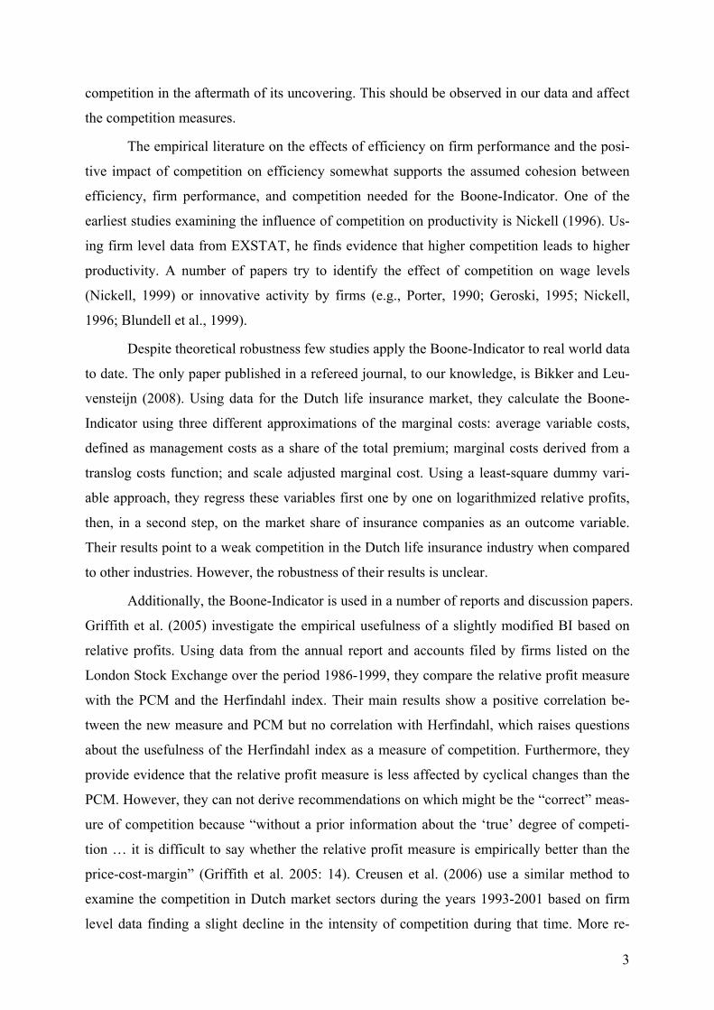
competition in the aftermath of its uncovering. This should be observed in our data and affect

the competition measures.

The empirical literature on the effects of efficiency on firm performance and the posi-

tive impact of competition on efficiency somewhat supports the assumed cohesion between

efficiency, firm performance, and competition needed for the Boone-Indicator. One of the

earliest studies examining the influence of competition on productivity is Nickell (1996). Us-

ing firm level data from EXSTAT, he finds evidence that higher competition leads to higher

productivity. A number of papers try to identify the effect of competition on wage levels

(Nickell, 1999) or innovative activity by firms (e.g., Porter, 1990; Geroski, 1995; Nickell,

1996; Blundell et al., 1999).

Despite theoretical robustness few studies apply the Boone-Indicator to real world data

to date. The only paper published in a refereed journal, to our knowledge, is Bikker and Leu-

vensteijn (2008). Using data for the Dutch life insurance market, they calculate the Boone-

Indicator using three different approximations of the marginal costs: average variable costs,

defined as management costs as a share of the total premium; marginal costs derived from a

translog costs function; and scale adjusted marginal cost. Using a least-square dummy vari-

able approach, they regress these variables first one by one on logarithmized relative profits,

then, in a second step, on the market share of insurance companies as an outcome variable.

Their results point to a weak competition in the Dutch life insurance industry when compared

to other industries. However, the robustness of their results is unclear.

Additionally, the Boone-Indicator is used in a number of reports and discussion papers.

Griffith et al. (2005) investigate the empirical usefulness of a slightly modified BI based on

relative profits. Using data from the annual report and accounts filed by firms listed on the

London Stock Exchange over the period 1986-1999, they compare the relative profit measure

with the PCM and the Herfindahl index. Their main results show a positive correlation be-

tween the new measure and PCM but no correlation with Herfindahl, which raises questions

about the usefulness of the Herfindahl index as a measure of competition. Furthermore, they

provide evidence that the relative profit measure is less affected by cyclical changes than the

PCM. However, they can not derive recommendations on which might be the “correct” meas-

ure of competition because “without a prior information about the ‘true’ degree of competi-

tion … it is difficult to say whether the relative profit measure is empirically better than the

price-cost-margin” (Griffith et al. 2005: 14). Creusen et al. (2006) use a similar method to

examine the competition in Dutch market sectors during the years 1993-2001 based on firm

level data finding a slight decline in the intensity of competition during that time. More re-

3

cently, the Finnish Ministry of Trade and Industry studied trend changes in the intensity of

competition across Finnish business sectors (Malirante et al. 2007). The report focuses on the

service sector and reports the results of nine different measures of competition including tradi-

tional measures like Herfindahl, PCM and the four-firm concentration index as well as six

different parameterizations of the Boone-Indicator. Their results suggest an increase in com-

petitive pressure in Finland in the analyzed time interval. However, the outcomes vary a lot

with respect to the different parameterizations of the BI and they state that “…the optimal

specification and estimation of the Boone indicator remains an open question and should thus

be debated.” (Malirante et al. 2007: 23)

We organize this paper as follows: In Section 2 we present the Boone-Indicator and

compare its theoretical robustness to the traditional PCM measure. In Section 3 we list the

relevant cartel cases in the power cable sector, the cement sector, and the ready mix concrete

sector. In Section 4 we give a detailed description of the dataset and present first descriptive

statistics. In Section 5 we discuss the Boone-Indicator and propose a modification to control

for firm size and present the main results of our analysis. Finally, in the last section we collect

the main findings and conclude the paper.

2. Measuring Competition

A common competition measure is the Lerner-Index or Price Cost Margin (PCM). It is based

in neoclassic theory where under perfect competition prices p equal marginal costs c .

Hence, the PCM, calculated as i ip c p i , takes values greater than zero if competition is not

perfect and firms are able to enforce prices above marginal costs. As competition becomes

fiercer PCM approaches zero. To evaluate competition on markets or in industries, the indus-

try PCM is calculated as a simple or weighted mean of individual PCMs. The latter is usually

derived by calculating it with firm market shares. This ensures that the market power of big

firms is adequately captured. The common interpretation is as with firm individual PCM. It

decreases with fiercer competition and increases with weaker competition.

However, it is not a robust competition measure. Amir (2003) shows that, under cer-

tain conditions, an increase in competition through an increase in the number of firms in a

market can result in an increasing average PCM. Given certain circumstances Stiglitz (1989)

shows that profits per unit sales can rise in a recession. Thus, even though competition among

firms increases during recessions, industry PCM also increases. Another potential source of

error can be the reallocation effect. As a result of fiercer competition, the market share of the

more efficient firms increases while that for less efficient firms decrease. Thus, the weighted

4

average PCM can increase if the increase in the market share of the more efficient firms over-

compensates the decrease of the respective individual PCMs. Therefore, the Lerner-Index is,

at least theoretically, potentially misleading.

Against this background and the fact that the interpretation of popular concentration

indices like Herfindahl is also not straightforward in terms of competition, Boone (2008a)

proposes a new competition measure. Termed Relative Profit Differences (RPD), its main

idea is that competition rewards efficiency. To get the measure working, Boone postulates

some assumptions of which the most important ones are outlined here. First, firms under con-

sideration act in a market with relatively homogeneous goods. Secondly, we assume symme-

try. Hence, firms act on a level playing field that ensures that changes in competition affect

firms directly and not indirectly through changes in that playing field. It also implies that

“…firm i’s profits are the same as firm j’s profits would be if firm j was in firm i’s situation.”

(Athey/Schmutzler 2001: 5). Thus, within the theoretical framework of the indicator, this im-

plies equal profit level for two equally efficient companies. Thirdly, we are able to rank firms

with respect to their efficiency in . Thereby the efficiency index N needs to be one dimen-

sional to ensure transitivity. Given that the production costs are captured by ,C q n with as

output quantity, the relationship between efficiency and cost is assumed to be:

q

1

,,0

and 0 for 1,2, ,,

0

ll

C q nC q n

qql L

nC q n

n

The proposition of the first two quotients on the left-hand side is clear-cut. The first

states that firms have positive marginal costs. The second quotients defines that costs are

lower the more efficient firms are. Finally, the quotient at the right-hand side states that mar-

ginal costs are lower for more efficient firms. Given these assumptions, firms play a two stage

game. In the first stage, they decide whether or not to enter. This is determined by the entry

costs and the expected profit. Only firms enter that are able to recoup entry costs. In the sec-

ond stage, the remaining firms simultaneously choose their actions to maximize profits. This

gives a subgame equilibrium for each competitive state.

1 Boone (2008a)

5

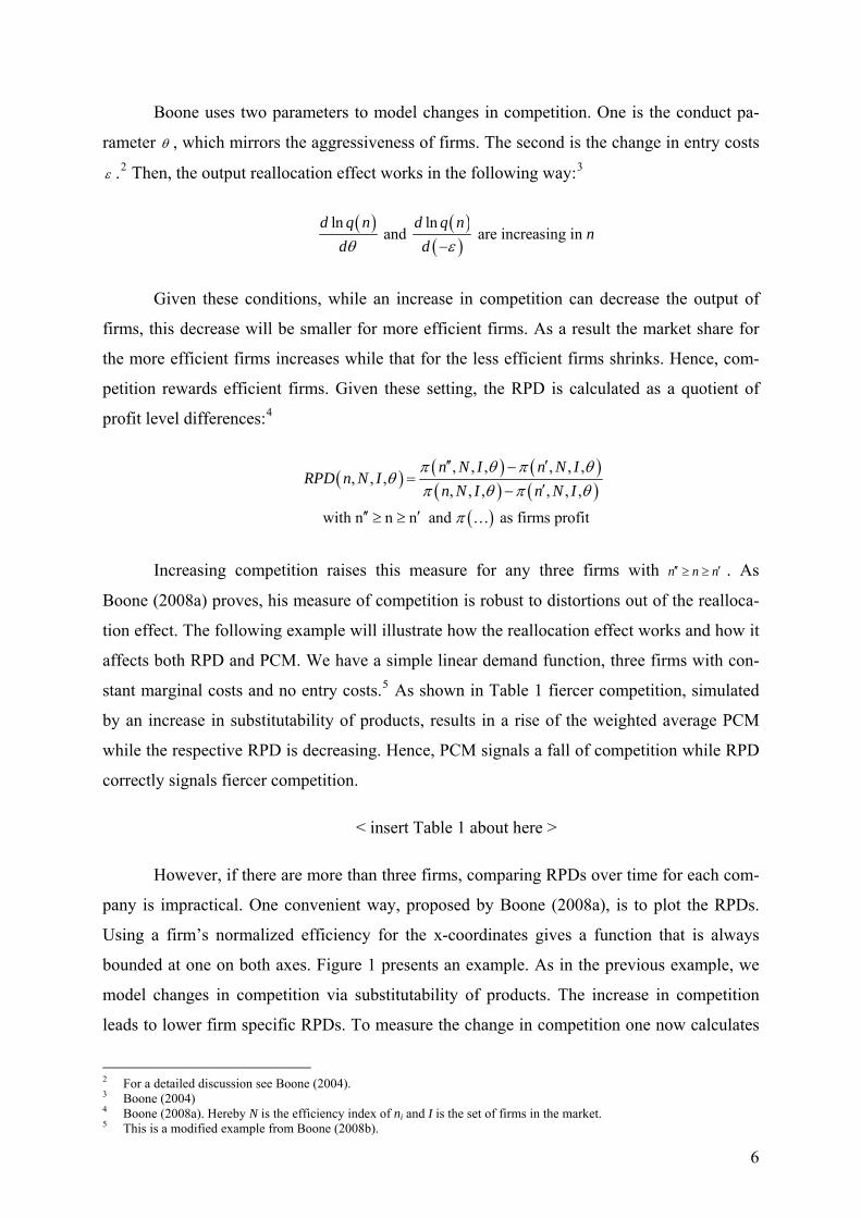
Boone uses two parameters to model changes in competition. One is the conduct pa-

rameter , which mirrors the aggressiveness of firms. The second is the change in entry costs

.2 Then, the output reallocation effect works in the following way:3

ln lnand are increasing in

d q n d q nn

d d

Given these conditions, while an increase in competition can decrease the output of

firms, this decrease will be smaller for more efficient firms. As a result the market share for

the more efficient firms increases while that for the less efficient firms shrinks. Hence, com-

petition rewards efficient firms. Given these setting, the RPD is calculated as a quotient of

profit level differences:4

, , , , , ,, , ,

, , , , , ,

with n n n and as firms profit

n N I n N IRPD n N I

n N I n N I

Increasing competition raises this measure for any three firms with n n . As

Boone (2008a) proves, his measure of competition is robust to distortions out of the realloca-

tion effect. The following example will illustrate how the reallocation effect works and how it

affects both RPD and PCM. We have a simple linear demand function, three firms with con-

stant marginal costs and no entry costs.

n

5 As shown in Table 1 fiercer competition, simulated

by an increase in substitutability of products, results in a rise of the weighted average PCM

while the respective RPD is decreasing. Hence, PCM signals a fall of competition while RPD

correctly signals fiercer competition.

< insert Table 1 about here >

However, if there are more than three firms, comparing RPDs over time for each com-

pany is impractical. One convenient way, proposed by Boone (2008a), is to plot the RPDs.

Using a firm’s normalized efficiency for the x-coordinates gives a function that is always

bounded at one on both axes. Figure 1 presents an example. As in the previous example, we

model changes in competition via substitutability of products. The increase in competition

leads to lower firm specific RPDs. To measure the change in competition one now calculates

2 For a detailed discussion see Boone (2004). 3 Boone (2004) 4 Boone (2008a). Hereby N is the efficiency index of ni and I is the set of firms in the market. 5 This is a modified example from Boone (2008b).

6

and compares the area under both curves. Since we have normalized values the area is

bounded between zero and one, with zero implying perfect competition and one the complete

absence of competition. The area in our example shrinks and thus correctly indicates fiercer

competition.

< insert Figure 1 about here >

3. Cartel Cases

In order to evaluate the robustness of the Boone-Indicator we use a natural experiment of

three major cartel cases in different sectors. A cartel is defined as an explicit contractual

agreement between legally independent companies in order to restrict competition and in-

crease profits. Such contracts define the prices, quantities, markets, etc., for each participating

firm. Further the contracts also implement a system of sanctions to ensure that deviant behav-

ior by cartel members is properly punished. Sometimes establishing a cartel includes the for-

mation of an organization that coordinates and monitors participating firms.

In addition to explicit cartels, there is also collusive behavior. This is characterized by

the absence of contractual agreements or any form of record. Instead it often relies on infor-

mal and mostly oral agreements. Although it has the same objective as a cartel, it usually can-

not restrict competition as effectively since firms have incentives to deviate from the collusion

strategy and the sanction mechanism is missing.6 However, since this way of restraining com-

petition is hard to detect we only focus on cartels.

For the purpose of our analysis cartels have to meet three criteria. Firstly, the cartel

must be nationwide. This ensures that it was able to restrict competition all over Germany.

Second, it must have been a cartel case of significant size. Hence, the cartel actually must

have gained a significant control over the national market. Both criteria ensure that the effect

can be found in the data. We take the size of the cartel fine as a proxy for the level of the dis-

tortion of competition. Finally, the product of a cartel should be as homogenous as possible,

leaving as little room for product diversification and, thusly, price discrimination.

When such cartels are uncovered and terminated, we expect fiercer competition in

subsequent periods. This assumption does not imply that competition changes to perfect com-

petition, nor does it neglect the possibility of future informal oral agreements by the involved

companies. However, as previously noted, collusive behavior is less effective than explicit

cartels. Moreover, it would not be rational to take the risk of an explicit cartel in the first place 6 However, there are of course gaming strategies which lead to similar results, given certain well specified condition. See

for instance Bester (2004).

7

if collusion could restrict competition at the same extent from the very beginning. Therefore

we impose the weak assumption that competition is significantly higher in the aftermath of a

legal cartel case compared to the cartel period.

Power cable cartel

The first cartel that appears to be suitable for our analysis is the cartel of German power cable

producers. It was constructed as a price- and quota-cartel, where producers agreed not only on

global market shares but also on shares for every big customer within a precisely defined pe-

riod and on the respective price range. In order to govern the cartel the “Elektro-Treuhand

GmbH” (ETG) was founded as a joint venture of all involved producers. The mechanism

worked in the following way: Every customer query was reported to the ETG. Since ETG also

did the cartel accounting, it knew which firms already were at quota during any given time

period, and which were not. They passed price- and discount-information to the companies

involved to ensure that in the following negotiations those companies scheduled to get the job

succeeded at the defined price. The cartel controlled the entire power cable market for several

decades. (Fleischhauer, 1997; Drucksache 14/1139).

The cartel ended in September 1996 in a nationwide search and seizure by the Federal

Cartel Office. By the end of 1997 the cartel office had charged 16 companies, two cable in-

dustry organizations and 28 individuals with a fine of 280 million Deutsch Mark (143 million

Euros) in total, the largest fine in German history at that time. All companies, except one,

accepted the fine and thus acknowledged having participated in an illegal cartel in order to

avoid competition. The organizational structure of the cartel was terminated, including the

closure of the ETG and the two cable industry organizations (Drucksache 14/1139).

Cement cartel

The second cartel in our analysis is the German cement cartel. It was created in the aftermath

of the German unification in the early 1990s as a price-, quota- and regional cartel covering

the entire German market for cement including importation (Pressemitteilung 19/09). All ma-

jor players and also medium sized producers took part in the cartel. Due to the physical prop-

erties of cement, which leads to excessively high transport costs over 300 kilometers, the

market for cement is regional. However, all players agreed on a nationwide organization of

regional cartels with explicit organizations for each regional market. The German market was

divided into an east, west, north and south submarkets. At this level the organizational struc-

ture varied. However, in each submarket contractual agreements were made (VI-2a Kart 2 -

6/08 OWi). The nationwide monitoring was done by the umbrella association of the German

cement producers (“Bundesverband der Deutschen Zementindustrie e.V.”). In the event that

8

cement was delivered outside a firm’s home market, compensatory payments were arranged

during ad hoc meetings held in Munich, the so-called “Money-Karussell” (money-carousel).

The cartel ended in July 2002 in a nationwide search and seizure of 30 companies. By

the end of 2003 the Federal Cartel Offices levied twelve companies and several persons with a

cartel fine of 702 million Euros in total (Drucksache 15/5790). However the companies under

suspicion, save for the company acting as principal witness, protested the amount of the fine.

The legal disputes lasted until June 2009 when the court finally confirmed all allegations but

reduced the fine to 330 million Euros. However, with respect to market effects we can state

two things. First, as stated by the court, witnesses, and various experts in the legal case, the

consequence of the uncovering of the cartel was a price war that lasted at least until 2005.

Second, to gain more information for the court, a second national seizure was carried out in

2004. There was no evidence whatsoever that the cartel still operated. Hence, the market con-

dition changed toward more competition. Blanckenburg and Geist (2009), confirm this, find-

ing fiercer competition after 2002.

Ready-mix concrete cartel

The last cartel case used in this study is that of the ready-mixed concrete industry. This was

actually not one cartel but many regional cartels. This is because the physical properties of

ready-mixed concrete limits transport time to roughly 60 minutes after a truck is filled.7 How-

ever, the entire German market was governed by regional cartels. The cartels were organized

as quota-cartels that specified the share for each participating firms within the regional market.

As typical for illegal cartels, regular meetings were established in order to monitor and govern

the activities of all involved parties, as for instance proved in the case of the Berlin ready-

mixed concrete cartel (KRB 2/05). As established by the courts, most cartels in the West were

formed around 1990, the ones in East Germany around 1995 (Drucksache 14/6300; Drucksa-

che 15/1226).

The first cartel was uncovered in May 1999 in Greater Berlin. Additional cartel in-

quests were opened against companies in the federal states of Sachsen-Anhalt and Nieder-

sachsen. Consequently the Federal Cartel Office initially charged 69 companies in 29 consor-

tiums with a cartel fine of 370 million Deutsch Mark (189 million Euros). With evidence

found in these cases and additional information, the cartel office carried out a nationwide

search and seizure of 48 companies in March 2000. Moreover, as a result of the cartel inquiry

on the cement market, some of the cement companies cooperated with cartel offices and

7 This information comes from the umbrella association of German ready-mix concrete industry. For further information

on the specifics of ready-mixed concrete market see also Syverson (2008)

9

passed further information about the ready-mixed concrete regional cartels to the authorities.

This allowed the authorities to open new cases against 70 ready-mixed concrete companies all

over Germany. The legal dispute lasted until 2005 when the Federal Supreme Court followed

the Federal Cartel Office in all main cases and stated that the participating companies had

established and operated illegal cartels, with the last cartel uncovered in 2001. (Drucksache

16/5710; KRB 2/05). Thus, roughly 140 companies were convicted with a fine of approxi-

mately 167 million Euros.

In the meantime the sector saw major changes. On the one hand, due to high overca-

pacity many companies closed (Drucksache 16/5710). Two major players, Larfarge and Han-

son, completely stopped its market engagement. Moreover, the Cartel Office approved 136

mergers between 2002 and 2006, which were seen as a result of a fierce competition while the

market struggled with overcapacities and declining sales. Moreover, State and Federal Cartel

Offices approved structural-crisis-cartels or cartels of small and medium-sized enterprises

under supervision of the cartel authorities (“Mittelstandskartell”) in some regional market in

order to support the regular capacity reduction and the process of adjusting to the new market

conditions (Drucksache 15/1226; Drucksache 15/5790; Drucksache 16/5710).

These three cartels meet our defined analysis needs. Each was large enough to influ-

ence competition at the national level and included all major suppliers and producers while

producing homogenous goods. All three cartels had illegal organizational structures and for-

mal cartel agreements needed to coordinate participating firms. Hence, it is expected that col-

lusion without such a structure is not as effective. Therefore, we expect fiercer competition

without such an organizational structure. Finally, all were heavily fined due to the extent of

the distorted competition.

4. Data

The data is taken from the German Cost Structure Census (Kostenstrukturerhebung) and the

German Production Census (Produktionserhebung). Each dataset was gathered and complied

by the German Statistical Office (Statistisches Bundesamt) over the period 1995-2006. Plant

level data is merged to firm level data using a common identifier. The strength of the dataset

is its sample coverage and reliability of information. It covers almost all large German manu-

facturing firms with 500 or more employees over the entire time span. Firms with fewer than

500 employees are included as a random subsample that is designed to be representative for

10

the small firm segment as a whole in every industry.8 Only firms with 20 or more employees

are covered.9

The Cost Structure Census contains information on several input categories, namely

payroll, employer contributions to the social security system, fringe benefits, expenditures for

material inputs, self-provided equipment, goods for resale, energy costs, external wage-work,

external maintenance and repair, tax depreciation of fixed assets, subsidies, rents and leases,

insurance costs, sales tax, other taxes and public fees, interest on external capital as well as

“other” costs such as license fees, bank charges and postage, or expenses.10 Finally, the Ger-

man Production Census gives detailed information about the number of products produced,

approximated by the nine-digit product classification system (Güterverzeichnis für Produk-

tionsstatistiken) of the Federal Statistical Office. This variable gives us as an important ele-

ment to identify the relevant sectors.

All previously mentioned studies followed Boone (2008a) and analyzed the competi-

tion based on three digit sector classification. With our rich dataset we are able to focus on a

four digit sector and goods classifications, defining the respective markets even more detailed

than any previous analysis. As discussed above, these are the power cable sector (WZ 3130),

the cement sector (WZ 2651) and the ready-mix concrete sector (WZ 2663). Each of these

sectors is characterized by a relatively homogeneous good. In order to guarantee relatively

comparable companies, we only look at companies which have at least 75 percent of their

overall turnover in one of these sectors. All other companies are dropped.

The sample contains a number of observations with extreme values that proved to im-

pact the calculation of the PCM and the estimation of the Boone-Indicator. Therefore, we ex-

clude observations from the analysis for which the cost for a certain input category in relation

to gross value added fall in the upper or lower one percentile of the sample per year.

According to Boone, we calculate profit by subtracting variable costs from revenue.

Hereby, we define revenue as revenue out of self produced goods. Hence, it does not include

revenues out of other activities like renting or trading operations. The variable costs contain

‘consumption of raw materials’, ‘energy’, ‘gross wages’, ‘legal and additional social insur-

ance contributions’, ‘costs for contract workers’ and ‘costs of repairs’. Following Boone

(2008a) we calculate two different measures for efficiency, i) average variable costs, which

we define as total variable costs per sales and ii) labor productivity, defined as gross value

8 Samples are drawn in 1995, 1997, 1999 and 2003. 9 In some particular industries, even firms with less than 20 employees are included as a random draw. 10 For more information about the Cost Structure Census surveys in Germany, we refer the reader to Fritsch et al. (2004).

11

added per employee. Additionally we also use sales per employee as a third measure for effi-

ciency. Descriptive statistics for the variables are presented in Table 3.

5. Empirical Investigation

We present our analysis in three steps. First, we present the parametric approach to apply

Boone’s idea and discuss its main drawbacks. In a second step we apply the Boone-Indicator

as theoretically defined on real data. We discuss its drawbacks and propose an augmented

indicator correcting for firm size. Finally, we use the above described cartel cases as natural

experiments to test for the empirical applicability of the Boone-Indicators and compare its

performance with that of the traditional PCM.

5.1. Discussion and Modification of the Boone-Indicator

Before the indicators are tested using the cartel cases, we briefly discuss the applicability of

the indicator on real word data. Griffith et al. (2005) was the first to propose a regression of

average variable costs on logarithmized profits. This is based on the idea behind the Boone-

Indicator that the more efficient a company becomes the greater the profit should be, ceterus

paribus. Since marginal costs are unobservable, average variable costs (AVC), defined as

total variable costs divided by sales, are taken as a crude proxy for marginal costs. They are

also used to assess firm efficiency. The estimated beta-coefficient measures the profit elastic-

ity of the respective firms. More precisely, “…it measures the percentage decrease (increase)

in firm i’s profit if its variable costs (i.e. marginal costs relative to price) increase (decrease)

by one percentage point.” (Griffith et al. 2005: 6). Since the relationship between profits and

average variable costs must be negative, the estimated coefficient needs to be negative. As

competition intensifies, the slope of the regression should become even more steeply negative,

following the idea that inefficient firms are punished more harshly by fiercer competition.

Although we will calculate RPDs, we also adopt this approach for comparative pur-

pose. However, we follow Creusen et al. (2006) and estimated the elasticity by means of

yearly log-log regressions: ln lnijt jt ijt ijtAVC with year, firmt i and . Then

the coefficient plainly gives the percentage change in profits due to a one percent change in

average variable costs. As shown by Boone et al. (2007) with simulations within his theoreti-

cal framework, changes in competition are correctly identified by this model.

=marketj

However, measuring competition this way can cause the usual problems for regression

analysis. The problems are well known and therefore we just want to mention one problem

directly related to the desired analysis. One task in that analysis is the definition of markets.

12

The more precisely we can capture a market, the less other factors or markets influence the

outcome and the better the subsequent competition estimates should be. On the other hand,

the more precisely we size a market, the fewer observations we will have. Moreover, markets

with few players are of special interest for competition analysis, but fewer observations de-

crease stability of regressions. An outlier can have a significant impact on the slope and the

significance of the coefficient (Urban and Myerl 2008).

A second problem is related to firm size. As long as we operate under the model’s as-

sumptions, the most efficient firm must become the biggest firm in terms of market share and

consequently, due to its efficiency level, it also must make the greatest profit. With respect to

linear regression analysis we must consider that in reality big firms are not necessarily the

most efficient ones and thus, it is possible to find a nonnegative beta-coefficient.11

In addition to the regression analysis that is usually used to apply the Boone idea on

real data, this paper tries to estimate the RPDs. Initially we assess the efficiency of firms in a

one-dimensional and transitive way. Following Boone (2008a) we use the average variable

costs, defined as total variable costs per sales TVC sales and labour productivity, defined as

gross value added per employee VA employee as efficiency index N. We add sales per em-

ployee sales employee as a third measure. Than the RPDs are calculated for each market (j) and

each firm (i) in every year (t) as:

with 1, , , 1, , and 1, ,ijt ijtijt

ijt ijt

n nRPD n t T j J i I

n n

,

where profits are defined as sales minus total variable costs ijt ijt ijtS TVC . The RPD

can only take values between zero and one, with one for the most efficient and zero the least

efficient firm. The efficiency of the firms is normalized via n n n n .

As the example in Figure 2 reveals, which depicts the RPDs for the cable industry (4

digit classification) in 2006, plainly applying this model on real world data is not sufficient.12

The RPDs are located between roughly 30 and -1, while we should see a scatter plot within

the boundaries of zero and one. We do have the most efficient firm located at the coordinate

(1,1) as it should be. However that firm has a profit below many of its competitors and it fol-

lows . Thus, the RPD can take values above one for less effi- ijt ijt ijt ijtn n n n

11 That both, size and few observations can have an impact is not just a theoretical problem as the results of Griffith et al.

(2005) show. 12 In this example the efficiency is defined by average variable costs. However, we can show further examples with labour

productivity.

13

cient firms. At the same time we have a least efficient firm, which has a profit above that of

other firms, resulting in negative numerators for these observations.

< insert Figure 2 about here >

This happens due to firm size. Obviously in the real world there are firms that are

really efficient, no matter of how efficiency is captured, but they can be small, at least at cer-

tain point in time. On the other hand, large companies may not be as efficient, but because of

the larger size, the firms make larger profits. To overcome this problem the RPD must be cal-

culated taking firm size into account. This can be done by means of number of employees or

sales. However, applying workforce to normalize profits does not give a good fit. We still

have RPDs significantly below zero and above one (Table 2), regardless of the efficiency in-

dex used. This might be caused by a weakness of the data set. It lacks information about the

number of temporary workers and for how long they stayed in the company, but we know

through a costs category that some firms used temporary workers. This biases the profits for

the respective firms as well as the efficiency if labour productivity and sales per employee is

applied. Therefore we do not use workforce in the calculation of the efficiency or to normal-

ize profits. Instead, in the subsequent analysis profits will by normalized by sales, which is

turnover out of the core business without trading or other activities. Thus, the RPD is calcu-

lated as:

ijt ijt ijt ijtijt

ijt ijtijt ijt

n sales n salesRPD n

n sales n sales

For the efficiency index we apply the average variable costs. In order to estimate the

area under each curve we use the Data Envelopment Analysis (DEA). It is a nonparametric

method that envelops the scatter plot at its outer boundary. We abstain from presenting the

method here and refer the interested reader to Canter et al. (2007) for a concise introduction

and to Simar and Wilson (2005) for a detailed discussion. Given the estimated curve we are

able to derive the corresponding area by integration.

5.2. Results

Given the above defined RPD we proceed with testing the validity of the Boone-Indicator

using the cartel cases. For this end we estimate the PCM of each firm as proposed by Boone

(2008a), and aggregate them into yearly industry PCMs using market share as the weight. The

market share is derived as the share of the firm sales on industry sales in a year. Further, we

14

estimate the BI as beta coefficients of the above outlined regression approach (afterwards also

called parametric indicator). Finally, we calculate the modified RPDs and the respective areas

as discussed above (also called nonparametric indicator). The change in competition is meas-

ured by subtracting the respective indicator in the base period from itself in the reference pe-

riod. Regardless of the indicator under consideration, a positive result shows an increase in

competition between the periods. A negative result on the other hand indicates decreasing

competitive pressure over time.

We used Welch’s t-test for evaluating the significance of changes in PCM since it ac-

counts for unequal variances in two samples. The same test is applied when comparing the

beta coefficients. However, the test can only be applied if both of the beta coefficients are

significant on there own. Otherwise, we depict just the difference labelling it as not significant.

Since the level of competition by means of RPDs is measured as area, tests based on means

and variances can not be applied. Therefore, the significance of differences between the areas

is calculated applying the nonparametric Wilcoxon rank-sum test on the underlying RPDs.

Given the estimates and tests, we can use the cartel events to derive the validity of the

indicators. As discussed in section 3 we expect fiercer competition in the aftermath of the

uncovering of a cartel. Hence, we look at the estimated changes in competition after such an

event compared to periods before the event. When possible, we look at the three years after

and the three years before the cartel case. The year of the event is not taken into consideration,

because the effect on the competition level in that year is not straightforward since we only

have annual data. The relevant biannual differences are presented in Table 4 to Table 6.

The first cartel we take a look at is the cable cartel. The cartel was uncovered in 1996.

Due to time limitations in our dataset we can only compare the changes in competition be-

tween 1995 and 1997 to 1999. Looking at the Lerner Index (Table 6), in all of the respective

biannual comparisons we see positive differences where two out of three of these differences

are significant. Thus, the PCMs indicate the expected increase in competition. The nonpara-

metric measure (Table 5) also indicates fiercer competition in the years 1997 to 1999 com-

pared to 1995, although just one of the differences is significant. The differences in elasticities

(Table 4) on the other hand are positive and negative, thus signalling decrease and increase in

competition after the cartel was terminated. However, the betas are not significantly different.

This is caused by the fact that the beta coefficient in 1995 is not significant at a 10 percent

level. Even if we ignore this fact and test for significant differences in betas, we find all chan-

ges to be significant, not only the positive difference. Thus with respect to the aim of this pa-

per we must state that PCM and the nonparametric indicator behaved as expected, indicating

15

fiercer competition in the aftermath of the termination of a cartel. In contrast, the parametric

indicator did not behave as expected.

Looking at the cement cartel, we find similar results as for the cable cartel. As dis-

cussed above, the cartel was uncovered in 2002, thus, we evaluate the changes in competition

of the period 1999 to 2001 against 2005 to 2006.13 Again, the weighted PCMs signal fiercer

competition after the event, where all results are significant. Yet, it is now the parametric in-

dicator signaling fiercer competition without exception and with all changes significant. To a

certain degree the area changes also indicate fiercer competition. Unfortunately none of the

changes are significant. Thus, although we only find positive values indicating fiercer compe-

tition, with the absence of significance we must record that the nonparametric indicator shows

no change in competition after the cement cartel was terminated.

Finally we look at the ready-mixed concrete cartels, where the first one was uncovered

in 1999 while the last one stopped its activity in 2001 as discussed before. We therefore de-

fine the period 1996 to 1998 as base period and 2002 to 2004 as reference period. As pre-

sented in Table 6, the PCMs differences again show the expected sign and are all significant.

The parametric indicator on the other hand is pointing to the opposite direction. All differ-

ences are negative and at least two are significant. If we overlook the insignificants of the

2003 and 2004 betas and test for differences, six out of nine negative differences would be

significant. The parametric indicator actually suggests weaker competition in the aftermath of

the termination of the ready-mixed concrete cartels. The nonparametric indicator is not per-

forming better. Although seven out of nine biannual comparisons are positive, pointing to-

ward fiercer competition, two are negative and no change is found to be significant.

< insert Figure 3 about here >

Figure 3 summarizes the main findings, depicting the direction of changes in competi-

tion with and without taking the significance of the changes into account. Here it is especially

interesting that the parametric Boone measure points just once in the expected direction, re-

gardless of significance. The nonparametric indicator, on the other hand, fails just once if we

ignore significance. Indeed, if we look closely at that unexpected outcome we find seven bi-

annual differences out of nine signalling fiercer competition, thus pointing into the expected

direction.

13 There are to few observations in 2003 and 2004 after running the outlier detection, so that we could not use this years due

to the data protection rules of the FDZ.

16

6. Conclusion

Using a rich newly built data set for German manufacturing enterprises, we test the empirical

validity of the Boone-Indicator. This is a new competition measure that, from its theoretical

properties, proved to be more robust than the Lerner-Index (also called PCM). The proof of its

empirical practicability and robustness is missing, however. This paper aims to shed light on

that question. To this end we use large cartel cases as events to compare the indicated compe-

tition levels before and after a cartel was uncovered and stopped operating. Since all of the

chosen cartels significantly restricted market competition, we expected fiercer competition in

the aftermath of the debunking of a cartel.

In the actual analysis we compare the performance of three competition measures. The

first is the Lerner-Index as a classical measure of competition. The second is the Boone-

Indicator calculated as beta coefficient of a log-log regression, as proposed by Boone et al.

(2007) and various other authors. Finally the Boone-Indicator derived by means of Relative

Profit Differences (RPD) is calculated using real data for the first time.

Our analysis reveals that the latter cannot be applied to real data as theoretically de-

fined. This is because the relationship between the efficiency of a firm and its profit level is

not as designed in Boone’s theoretical framework, where the most efficient company is al-

ways, by design, the biggest firm in terms of market share. Our results suggest that this rela-

tionship does not hold in reality. Therefore we propose a way to account for firm size in the

calculation of RPDs.

With respect to the performance of the indicator in the face of uncovered cartels we

note that the Lerner-Index performed as expected. In every case it indicated fiercer competi-

tion in the aftermath of a cartel case with almost all biannual comparison to be significant.

Hence, although not theoretically robust, in this analysis it proved its empirical usefulness.

This we cannot state for the two Boone-Indicators, in particular the regression approach. Re-

gardless of whether or not we account for the significance of changes and betas, the indicator

just once indicates fiercer competition. This supports our doubts regarding this approach. The

Boone-Indicator based on RPDs also does not perform as well as the Lerner-Index. This is

mainly because the changes are often not significant. Leaving significance aside, the Boone-

Indicator by means of RPD and taking firm size into account perform almost as well as PCM.

Based on our findings we conclude that the Boone-Indicator, although theoretically

superior, is, at least at this stage, not an empirically robust indicator. The Lerner-Index on the

other hand indicates changes in competition as expected. However, the results of the RPD

17

based Boone-Indicator are promising. Future research should focus on alternative methods to

account for firm size while keep the original variation of the profit levels.

18

References

Aghion, P., N. Bloom, R. Blundell, R. Griffith, P. Howitt (2005), Competition and Innovation: An Inverted-U Relationship. Quarterly Journal of Economics 120 (2): 701-728.

Amir, R. (2003), Market Structure, Scale Economies and Industry Performance. CORE Dis-cussion Paper Series 2003/65.

Athey, S., A. Schmutzler (2001), Investment and market dominance. RAND Journal of Eco-nomics 32 (1): 1-26.

Bikker, J.A., M. von Leuvensteijn (2008), Competition and efficiency in the Dutch life insur-ance industry. Applied Economics 40: 2063-2084.

Blundell, R, R. Griffith, J. van Reenen, (1999), Market share, market value and innovation in a panel of British manufacturing firms. Review of Economic Studies 66(3): 529-554.

Bundesgerichtshof, Beschluss vom 28. Juni 2005 – KRB 2/05 – OLG Düsseldorf. available at: http://juris.bundesgerichtshof.de/cgi-bin/rechtsprechung/list.py?Gericht=bgh&Art=en&Datum=2005-6&Seite=1 (download: 16.06.2009).

Bester, H. (2004), Theorie der Industrieökonomik. Berlin/Heidelberg.

Blankenburg, K. von, A. Geist (2009), How can a cartel be detected? International Advan-tages in Economic Research 15: 421-436.

Bulow, J., P. Klemperer (1999), Prices and the winner’s curse. RAND Journal of Economics 33(1): 1-21.

Boone, J. (2004), A new way to measure competition. Tilburg University, CentER Discussion Papers 2004-31.

Boone, J., J. van Ours, H. van der Wiel (2007), How (not) to measure competition. CPB Dis-cussion Paper No 91.

Boone, J. (2008a), A new way to measure competition. The Economic Journal 188: 1245-1261.

Boone, J. (2008b), Competition: Theoretical Parameterizations and Empirical Measures. Journal of Institutional and Theoretical Economics 164: 587-611.

Canter, U., J. Krüger, H. Hanusch (2007), Produktivitäts- und Effizienzanalyse: Der nichtpa-rametrische Ansatz. Berlin/Heidelberg.

Creusen, H., B. Minne, H. van der Wiel (2006), Competition in the Netherlands: An analysis of the period 1993-2001. CPB Document No 136.

Deutscher Bundestag, 14. Wahlperiode, Drucksache 14/1139, Unterrichtung durch die Bun-desregierung, Bericht des Bundeskartellamtes über seine Tätigkeit in den Jahren 1997/1998 sowie über die Lage und Entwicklung auf seinem Aufgabengebiet und Stel-lungnahme der Bundesregierung. available at: http://www.bundeskartellamt.de/wDeutsch/publikationen/Taetigkeitsbericht.php (downloaded: 16.06.2010).

19

Deutscher Bundestag, 14. Wahlperiode, Drucksache 14/6300, Unterrichtung durch die Bun-desregierung, Bericht des Bundeskartellamtes über seine Tätigkeit in den Jahren 1999/2000 sowie über die Lage und Entwicklung auf seinem Aufgabengebiet und Stel-lungnahme der Bundesregierung. available at: http://www.bundeskartellamt.de/wDeutsch/publikationen/Taetigkeitsbericht.php (downloaded: 16.06.2010).

Deutscher Bundestag, 15. Wahlperiode, Drucksache 15/1226, Unterrichtung durch die Bun-desregierung, Bericht des Bundeskartellamtes über seine Tätigkeit in den Jahren 2001/2002 sowie über die Lage und Entwicklung auf seinem Aufgabengebiet und Stel-lungnahme der Bundesregierung. available at: http://www.bundeskartellamt.de/wDeutsch/publikationen/Taetigkeitsbericht.php (downloaded: 16.06.2010).

Deutscher Bundestag, 15. Wahlperiode, Drucksache 15/5790, Unterrichtung durch die Bun-desregierung, Bericht des Bundeskartellamtes über seine Tätigkeit in den Jahren 2003/2004 sowie über die Lage und Entwicklung auf seinem Aufgabengebiet und Stel-lungnahme der Bundesregierung. available at: http://www.bundeskartellamt.de/wDeutsch/publikationen/Taetigkeitsbericht.php (downloaded: 16.06.2010).

Deutscher Bundestag, 16. Wahlperiode, Drucksache 16/5710, Unterrichtung durch die Bun-desregierung, Bericht des Bundeskartellamtes über seine Tätigkeit in den Jahren 2005/2006 sowie über die Lage und Entwicklung auf seinem Aufgabengebiet und Stel-lungnahme der Bundesregierung. available at: http://www.bundeskartellamt.de/wDeutsch/publikationen/Taetigkeitsbericht.php (downloaded: 16.06.2010).

Fleischhauer, J. (1997), Korrekte Buchhaltung. p. 100 in: Der Spiegel 24/1997.

Fritsch et al. (2004), Cost Structure Surveys for Germany. Schmollers Jahrbuch 124: 557-566.

Geroski, P. A. (1995a), Market structure, corporate performance and innovative activity. Oxford.

Griffith, R., J. Boone, R. Harrison (2005), Measuring Competition. AIM Research Working Paper Series 022-August-2005.

Klette, T. J. (1999), Market Power, Scale Economies and Productivity: estimates from a panel of establishment data. Journal of Industrial Economics 47(4): 451–476.

Maliranta, M., M. Pajarinen, P. Rouvinen, P. Ylä-Anttila (2007), Competition in Finland: Trends across Business Sectors in 1994–2004. Ministry of Industry, MTI Publications 13/2007.

Maudos, J., J. Fernadez de Guevara (2006), Banking competition, financial dependence and economic growth. Munich Personal RePEc Archive 15254.

Nevo, A. (2001), Measuring market power in the ready-to-eat cereal industry. Econometrica 69 (2): 307-342.

Nickell, S. (1996), Competition and Corporate Performance. Journal of Political Economy 140 (4): 724-746.

20

Nickell, S. (1999), Product markets and labour markets. Journal of Political Economics 6(1): 1-20.

Porter, M. E. (1990), The competitive advantage of nations, The Free Press, New York.

Pressemitteilung Nr. 19/09, Bußgeldverfahren „Zementkartell“ vor dem OLG Düsseldorf be-endet. OLG Düsseldorf, 29.06.2009. available at: http://www.justiz.nrw.de/Presse/presse_weitere/PresseOLGs/archiv/2009_01_Archiv/29_06_2209/index.php (downloaded: 16.06.2010).

Pruteanu-Podpiera, A., L. Weill, F. Schobert (2007), Market Power and Efficiency in the Czech Banking Sector. CNB Working Paper Series 6/2007.

Rosenthal, R. (1980), A model in which an increase in the number of sellers leads to a higher price. Econometrica 48(6): 1575-1579.

Simar, L, P.W. Wilson (2005), Statistical Inference in Nonparametric Frontier Models: Re-cent Developments and Perspectives. p. 1-125 in: Fried, H. C.A.K., Lovell, S.S. Schmidt (Eds.), The Measurement of Productive Efficiency Techniques and Application 2nd Edi-tion. Oxford.

Stiglitz, J. (1989), Imperfect information in the product market. p. 769-847 in: R. Schmalen-see, R. Willig (Eds.), Handbook of Industrial Organization Vol. I. Amsterdam.

Syverson, C. (2008), Markets Ready-Mixed Concrete. Journal of Economic Perspectives 22: 217-233.

Urban, D., J. Mayerl (2008), Regressionsanalyse: Theorie, Technik und Anwendung Vol. 3. Wiesbaden.

Urteil des 2a. Kartellsenat Oberlandesgericht Düsseldorf, Aktenzeichen VI-2a Kart 2 - 6/08 OWi, available upon request at the OLG Düsseldorf.

21

Appendix

Figure 1: Fiercer competition and RPD14

0

0,2

0,4

0,6

0,8

1

0 0,2 0,4 0,6 0,8 1

normalized efficiency

RP

D

Figure 2: RPDs for cable industry in 200615

0.0 0.2 0.4 0.6 0.8 1.0

05

10

15

20

25

30

normalized efficiency

no

rma

lize

d p

rofit

14 We apply the same demand function as in the example of table 1. We have 20 firms in the beginning with constant mar-

ginal costs of 10ic i . There are no entry costs, 20, 2a b and d increases from 0.1 to 2. The solid line captures the

RPDs in situation one, hence with low intense competition due to a d of 0.1, while the dotted line is with . To over-come the problem that appears if the least efficient firm is assessed, which means dividing by zero, we calculate inverse

RPDs, hence:

2d

, , , ,nn n n . The normalized efficiency is calculated as: n n n n

with n n n 15 The efficiency was measured by average variable costs.

22

Figure 3: change in competition after the termination of the cartels16

Event PCM Boon-Indicator PCM Boon-Indicator Industry (4-digit classification)

log. regression

RPD log. regression

RPD

power cable (3130) 1996 ↑* →* ↑* ↑ → ↑

cement (2651) 2002 ↑* ↑* →* ↑ ↑ ↑ ready-mixed con-

crete (2663) 1999-2002

↑* ↓* →* ↑ ↓ →

16 * marks the direction changes in competition that take significance into account.

23

Table 1: The reallocation effect and how it affects PCM and RPD17

PCM1 PCM2 PCM3 Weighted Industry

PCM

RPD3

d=0.1 0.950 0.587 0.465 0.680 0.262 d=2 0.939 0.385 0.139 0.717 0.149

Table 2: Mean absolute deviation of RPDs form the boundaries of One and Zero for different

efficiency measures and normalized profits18

labor productivity sales per employee total average variable cost sectors 2651 2663 3130 2651 2663 3130 2651 2663 3130 years profit normalized by number of employees 1995 0.15 0.144*** 0.122* 0.372** 0.068*** 0.128* - 0.293*** 0.03 1996 0.081 0.002 0.27 0.129 0.002 0.27 - 0.031 0.006 1997 0.389 0.027 0.139*** 0.389 0.027 0.139*** - 0.226*** 0.063 1998 0.041 0.39*** 0.348*** 0.041 0.39*** 0.348*** 0.124 0.045** 0.509*** 1999 0.411 0.014** 0.258 0.411 0.014** 0.258 - 0.026*** 0.881*** 2000 0.531 0.062** 0.154*** 0.531 0.062** 0.154*** 0.062 0.082 1.88*** 2001 0.158 0.02 0.316*** 0.158 0.02 0.316*** 0.126** 0.199** 1.214*** 2002 0.236 0.085** - 0.236 0.085** - - 0.04 0.088*** 2003 - 0.008** 0.02 0.008** 0.052 0.233* 2004 0.062** 0.084** 0.062** 0.088 0.53** 0.11** 2005 0.094 0.067** 0.065* 0.094 0.067** 0.075* 0.163 0.351** 0.071*** 2006 0.554* 0.03 0.011 0.554* 0.03 0.011 2.225* 0.326* 0.353*** years profit normalized by sales 1995 4.326*** 1.8*** 0.517*** 4.326*** 5.191*** 0.783*** - - - 1996 0.45** 0.477*** 1.018*** 0.45** 0.477*** 1.018*** - - - 1997 0.169 0.303*** 0.27*** 0.169 0.303*** 0.27*** - - - 1998 0.222*** 0.064*** 0.605** 0.222*** 0.064*** 0.605** - - - 1999 0.903** 0.541*** 13.839*** 0.903** 0.375*** 13.839*** - - - 2000 7.21*** 24.66*** 0.544*** 0.052 24.66*** 0.544*** - - - 2001 1.176*** 0.321*** 5.213*** 1.176*** 0.321*** 5.213*** - - - 2002 0.787** 6.764*** 0.759*** 0.787** 6.764*** 0.759*** - - - 2003 0.541*** 32.276*** 0.61*** 32.276*** - - 2004 2.585*** 0.292*** 2.585*** 1.615*** - - 2005 2.035 0.862*** 6.725*** 2.035 0.862*** 8.964*** - - - 2006 0.661 0.211 0.488*** 0.661 0.308 0.488*** - - -

Note: *** 1% significance level, ** 5% significance level, * 10% significance level, - no observation below

j

17 The demand function is 1,i ij i

p x x a bx d x

and is taken from Boone (2008b). We apply a=20, b=2 and

marginal costs are c1=0.5, c2=5 and c3=7. The substitutability is captured by d, where the quotient 1d b for perfect

substitutes. We do not report the RPD for the most and the least efficient firm since they have to be one and zero at both times by

definition. 18 The table shows the absolute mean deviation of observed RPDs. The t-test was applied to test the significance of the

deviation.

24

Table 3: descriptive statistics of applied variables

labor productivity sales per employee average variable cost profit per employee profit profit per sales years N mean stdev N mean stdev N mean stdev N mean stdev N mean stdev N mean stdev

1995 12 275941.51 129813.93 12 250929.88 135268.84 12 0.649 0.098 10 83120.21 28026.36 10 24654701.55 17453737.68 10 0.357 0.072 1996 14 265036.62 127948.35 14 249585.34 130711.21 14 0.629 0.105 12 88773.66 32464.45 12 22778734.13 15832666.98 12 0.377 0.076 1997 12 276189.53 145353.94 12 261612.75 150995.23 12 0.687 0.137 10 74634.88 39439.96 10 16802487.80 16717070.01 10 0.307 0.123 1998 15 278276.44 156382.50 15 270103.39 156462.29 15 0.698 0.168 13 76120.76 46540.80 13 14735482.19 15604300.49 13 0.303 0.155 1999 11 274748.10 134320.53 11 270853.22 131465.84 11 0.642 0.117 9 88671.80 41351.98 9 14200256.44 5614375.85 9 0.354 0.088 2000 10 288927.17 146704.66 10 282349.24 148575.94 10 0.636 0.128 8 88255.96 32752.75 8 13883868.00 6443732.38 8 0.365 0.102 2001 11 270489.54 119815.39 11 263364.86 119862.98 11 0.621 0.087 9 90750.26 36495.89 9 14446138.39 5230236.09 9 0.373 0.046 2002 10 245045.22 121731.84 10 236704.63 114060.71 10 0.697 0.143 8 67226.60 32639.25 8 11084038.59 5612858.25 8 0.295 0.118 2003 5 300541.35 149883.91 5 296174.19 140902.28 5 0.806 0.127 3 - - 3 - - 3 - - 2004 6 309138.85 164345.12 6 302090.05 155287.22 6 0.750 0.109 4 - - 4 - - 4 - - 2005 8 294208.58 130545.15 8 290029.69 131093.51 8 0.774 0.082 6 66548.27 36666.66 6 6636015.96 2810269.67 6 0.229 0.052

cem

ent (

2651

)

2006 9 324927.22 146052.86 9 316989.06 140402.72 9 0.789 0.092 7 65738.91 26572.20 7 6262759.34 4123335.23 7 0.212 0.063 1995 54 251117.62 129036.76 54 233626.90 101980.56 54 0.747 0.109 52 60371.38 38170.91 52 2616140.67 1988239.08 52 0.251 0.100 1996 53 254805.13 113837.36 53 244309.09 111584.94 53 0.753 0.093 51 61082.96 39192.39 51 2814139.71 2323074.70 51 0.246 0.085 1997 49 273992.96 123699.78 49 255339.73 120220.88 49 0.753 0.099 47 66414.15 42546.41 47 3313806.18 4237861.19 47 0.247 0.091 1998 48 279176.87 124248.85 48 261529.14 118127.47 48 0.765 0.090 46 64148.75 42623.48 46 3771510.86 4739668.24 46 0.233 0.081 1999 52 274033.77 116433.09 52 253774.86 107210.53 52 0.760 0.102 50 63797.39 38075.43 50 3210729.85 3239263.76 50 0.240 0.092 2000 42 251756.12 102335.12 42 233123.35 92110.32 42 0.789 0.086 40 46870.18 21091.43 40 2815013.48 2825058.13 40 0.208 0.075 2001 41 244960.06 98983.09 41 225744.35 85260.38 41 0.828 0.090 39 36569.27 19329.71 39 1822365.37 1883094.22 39 0.172 0.083 2002 34 241576.69 103036.93 34 225902.39 91855.19 34 0.810 0.089 32 40494.91 19379.63 32 2089801.49 1478034.08 32 0.188 0.080 2003 33 261039.86 162679.94 33 241767.11 159280.52 33 0.791 0.115 31 47589.03 32841.38 31 2120169.47 1820009.56 31 0.207 0.102 2004 28 264242.60 159316.55 28 245730.82 153393.66 28 0.771 0.101 26 55913.14 42054.17 26 2660461.54 2640251.05 26 0.227 0.089 2005 27 248869.77 160936.75 27 231151.24 156099.15 27 0.793 0.107 25 47970.41 35245.75 25 2294912.86 2396800.51 25 0.205 0.095

read

y-m

ixed

con

cret

e (2

663)

2006 25 262554.37 151372.94 25 243909.69 140061.37 25 0.776 0.101 23 52561.25 34258.02 23 2930521.63 3296418.43 23 0.222 0.082 1995 27 137050.79 81077.73 27 131736.93 77630.07 27 0.793 0.137 25 27518.89 25609.48 25 2837311.25 3734492.90 25 0.198 0.110 1996 32 125834.14 70994.28 32 122574.71 71751.78 32 0.800 0.130 30 24678.87 22063.71 30 2748478.84 4123596.11 30 0.193 0.109 1997 27 157486.33 112253.24 27 155005.09 112373.79 27 0.804 0.134 25 25687.72 17474.33 25 3780242.70 5024262.03 25 0.188 0.111 1998 27 175971.06 108371.88 27 171222.35 104395.73 27 0.804 0.119 25 28747.07 15826.69 25 3900144.49 4740320.96 25 0.191 0.099 1999 40 135041.67 95481.60 40 127359.11 91574.56 40 0.823 0.097 38 20127.21 14699.69 38 2613762.00 4875401.33 38 0.174 0.085 2000 46 143254.13 109120.80 46 134039.37 104077.61 46 0.809 0.109 44 22639.76 17189.35 44 3048404.80 6402232.59 44 0.183 0.079 2001 43 156818.27 112995.34 43 141924.92 103674.28 43 0.810 0.121 41 24764.81 20117.29 41 7958490.43 23292462.10 41 0.180 0.076 2002 39 120835.79 85302.58 39 113354.50 78258.16 39 0.813 0.089 37 20792.55 14417.71 37 2635375.63 5314750.34 37 0.187 0.083 2003 32 185344.88 113356.04 32 172921.88 108741.88 32 0.823 0.092 30 28691.09 20712.85 30 4294877.94 6179956.47 30 0.172 0.076 2004 33 184921.04 127967.38 33 169483.13 116443.65 33 0.839 0.083 31 24552.29 17225.56 31 3314602.39 4756077.99 31 0.157 0.068 2005 35 201946.92 145788.62 35 179365.03 128275.93 35 0.826 0.098 33 28986.68 21380.44 33 3395725.65 4787847.22 33 0.171 0.089

pow

er c

able

(31

30)

2006 37 221277.66 195301.91 37 197897.10 180639.40 37 0.827 0.092 35 28875.81 21964.10 35 3297811.57 4226426.49 35 0.171 0.080

25

Table 4: differences in beta over time

years 1996 1997 1998 1999 2000 2001 2002 2003 2004 2005 2006 1995 -1.039** -0.538 -0.521 -2.293*** -2.149*** -2.587*** -1.851*** - - -0.723 2.611*** 1996 - 0.501* 0.518* -1.254*** -1.11*** -1.548*** -0.812* - - 0.316 3.65*** 1997 - - 0.017 -1.755*** -1.612*** -2.049*** -1.313*** - - -0.185 3.149*** 1998 - - - -1.772*** -1.628*** -2.066*** -1.33*** - - -0.202 3.132*** 1999 - - - - 0.144 -0.294 0.442 - - 1.57** 4.904*** 2000 - - - - - -0.437 0.298 - - 1.426** 4.76*** 2001 - - - - - - 0.736* - - 1.864*** 5.198*** 2002 - - - - - - - - - 1.128* 4.462*** 2003 - - - - - - - - - - - 2004 - - - - - - - - - - -

cem

ent (

2651

)

2005 - - - - - - - - - - 3.334*** 1995 0.361*** 1.409*** 2.009*** 1.291*** -1.271 1.284*** 0.228 -1.13 -0.065 -0.144 -3.32 1996 - 1.049*** 1.648*** 0.931*** -1.632 0.924*** -0.132 -1.491 -0.426 -0.504 -3.68 1997 - - 0.6*** -0.118 -2.68 -0.125 -1.181*** -2.539 -1.474 -1.553 -4.729 1998 - - - -0.718*** -3.28 -0.725*** -1.78*** -3.139 -2.074 -2.152 -5.329 1999 - - - - -2.562 -0.007 -1.063*** -2.421 -1.357 -1.435 -4.611 2000 - - - - - 2.555 1.499 0.141 1.206 1.127 -2.049 2001 - - - - - - -1.056*** -2.414 -1.349 -1.428 -4.604 2002 - - - - - - - -1.358 -0.294 -0.372 -3.548 2003 - - - - - - - - 1.065 0.987 -2.19 2004 - - - - - - - - - -0.078 -3.255

read

y-m

ixed

con

cret

e (2

663)

2005 - - - - - - - - - - -3.176 1995 1.081 -0.859 -1.499 1.364 1.218 3.591 2.131 0.575 -0.53 0.677 -0.612 1996 - -1.94 -2.58 0.283 0.137 2.51*** 1.05*** -0.506 -1.611 -0.404 -1.694 1997 - - -0.64 2.223 2.077 4.050 2.989 1.434 0.329 1.536 0.246 1998 - - - 2.863 2.717 5.090 3.629 2.074 0.969 2.176 0.886 1999 - - - - -0.146 2.227*** 0.767* -0.789 -1.894 -0.687* -1.977 2000 - - - - - 2.373*** 0.912** -0.643 -1.748 -0.541 -1.831 2001 - - - - - - -1.461*** -3.016 -4.121 -2.914*** -4.204 2002 - - - - - - - -1.555 -2.661 -1.453*** -2.743 2003 - - - - - - - - -1.105 0.102 -1.188 2004 - - - - - - - - - 1.207 -0.083

pow

er c

able

(31

30)

2005 - - - - - - - - - - -1.29 Note: *** 1% significance level, ** 5% significance level, * 10% significance level

26

Table 5: spread between areas over time

years 1996 1997 1998 1999 2000 2001 2002 2003 2004 2005 2006 1995 -0.011 -0.016 -0.041 -0.01 -0.003 0.024 -0.015 - - 0.044 0.026 1996 - -0.005 -0.03 0.001 0.008 0.035 -0.004 - - 0.055 0.037 1997 - - -0.025 0.005 0.013 0.04 0 - - 0.06 0.042 1998 - - - 0.031 0.038 0.065 0.026 - - 0.085 0.068 1999 - - - - 0.007 0.034 -0.005 - - 0.054 0.037 2000 - - - - - 0.027 -0.012 - - 0.047 0.029 2001 - - - - - - -0.04 - - 0.02 0.002 2002 - - - - - - - - - 0.06 0.042 2003 - - - - - - - - - - - 2004 - - - - - - - - - - -

cem

ent (

2651

)

2005 - - - - - - - - - - -0.018 1995 0.007 0 0.02 0.014 0.015 0.022 0.029 0.011* 0.016 0.01 0.011 1996 - -0.006 0.013 0.008*** 0.009 0.015 0.022 0.005 0.009 0.003 0.005 1997 - - 0.02 0.014** 0.015 0.022 0.029 0.011 0.016 0.01 0.011 1998 - - - -0.006** -0.004 0.002 0.009 -0.008 -0.004 -0.01 -0.008 1999 - - - - 0.001*** 0.008 0.015 -0.003** 0.001** -0.005 -0.003** 2000 - - - - - 0.007* 0.014 -0.004 0 -0.006 -0.004 2001 - - - - - - 0.007 -0.011* -0.006 -0.012 -0.011 2002 - - - - - - - -0.018 -0.013 -0.019 -0.018 2003 - - - - - - - - 0.004 -0.002 0 2004 - - - - - - - - - -0.006 -0.004

read

y-m

ixed

con

cret

e (2

663)

2005 - - - - - - - - - - 0.002 1995 -0.014 0.01 0.014 0.041** 0.041 0.036 0.043* 0.052 0.052 0.032 0.031 1996 - 0.024 0.028 0.055*** 0.056*** 0.05** 0.058*** 0.066*** 0.066*** 0.047 0.045** 1997 - - 0.004 0.031** 0.031* 0.026 0.033** 0.042* 0.042* 0.022 0.021 1998 - - - 0.027*** 0.027** 0.021 0.029*** 0.038** 0.038** 0.018 0.017** 1999 - - - - 0 -0.005** 0.002 0.011 0.011 -0.009** -0.01* 2000 - - - - - -0.006 0.002 0.011 0.01 -0.009 -0.01 2001 - - - - - - 0.008* 0.016 0.016 -0.003 -0.005 2002 - - - - - - - 0.009 0.008 -0.011* -0.012* 2003 - - - - - - - - 0 -0.02 -0.021 2004 - - - - - - - - - -0.02 -0.021

pow

er c

able

(31

30)

2005 - - - - - - - - - - -0.001 Note: *** 1% significance level, ** 5% significance level, * 10% significance level

27

28

Table 6: changes in PCM over time

years 1996 1997 1998 1999 2000 2001 2002 2003 2004 2005 2006 1995 -0.018 -0.003 0.006 -0.008 -0.016 -0.007 0.05 - - 0.13*** 0.137*** 1996 - 0.015 0.024 0.01 0.002 0.011 0.068 - - 0.148*** 0.155*** 1997 - - 0.009 -0.005 -0.014 -0.004 0.053 - - 0.132*** 0.139*** 1998 - - - -0.014 -0.022 -0.013 0.044 - - 0.124** 0.13** 1999 - - - - -0.008 0.001 0.058 - - 0.138*** 0.144*** 2000 - - - - - 0.01 0.066 - - 0.146*** 0.153*** 2001 - - - - - - 0.057 - - 0.136*** 0.143*** 2002 - - - - - - - - - 0.08* 0.086* 2003 - - - - - - - - - - - 2004 - - - - - - - - - - -

cem

ent (

2651

)

2005 - - - - - - - - - - 0.007 1995 -0.004 -0.018 -0.008 0.006 0.047*** 0.093*** 0.079*** 0.08*** 0.042** 0.053*** 0.044** 1996 - -0.015 -0.005 0.009 0.051*** 0.096*** 0.082*** 0.084*** 0.045** 0.057*** 0.047*** 1997 - - 0.01 0.024 0.066*** 0.111*** 0.097*** 0.098*** 0.06*** 0.072*** 0.062*** 1998 - - - 0.014 0.056*** 0.101*** 0.087*** 0.088*** 0.05** 0.062*** 0.052*** 1999 - - - - 0.042*** 0.087*** 0.073*** 0.074*** 0.036* 0.048** 0.038** 2000 - - - - - 0.046*** 0.031* 0.033* -0.005 0.006 -0.003 2001 - - - - - - -0.014 -0.013 -0.051** -0.039** -0.049*** 2002 - - - - - - - 0.001 -0.037* -0.025 -0.035* 2003 - - - - - - - - -0.038* -0.027 -0.036** 2004 - - - - - - - - - 0.011 0.002

read

y-m

ixed

con

cret

e (2

663)

2005 - - - - - - - - - - -0.009 1995 -0.024 0.055* 0.057* 0.042 0.031 -0.017 0.041 0.053* 0.087*** 0.064** 0.087*** 1996 - 0.079** 0.081** 0.066** 0.056* 0.007 0.065** 0.077** 0.112*** 0.088*** 0.112*** 1997 - - 0.002 -0.013 -0.024 -0.072*** -0.014 -0.002 0.032* 0.009 0.032 1998 - - - -0.015 -0.026 -0.074*** -0.016 -0.004 0.03 0.007 0.03 1999 - - - - -0.011 -0.059*** -0.001 0.011 0.045*** 0.021 0.045*** 2000 - - - - - -0.049*** 0.009 0.021 0.056*** 0.032* 0.056*** 2001 - - - - - - 0.058*** 0.07*** 0.105*** 0.081*** 0.105*** 2002 - - - - - - - 0.012 0.047*** 0.023 0.047*** 2003 - - - - - - - - 0.035** 0.011 0.035** 2004 - - - - - - - - - -0.024 0

pow

er c

able

(31

30)

2005 - - - - - - - - - - 0.024 Note: *** 1% significance level, ** 5% significance level, * 10% significance level