Empirical analysis of natural gas markets - econstor

econstorMake Your Publications Visible.

A Service of

zbwLeibniz-InformationszentrumWirtschaftLeibniz Information Centrefor Economics

Anderson, David A. (Ed.); Hamori, Shigeyuki (Ed.)

Book — Published Version

Empirical analysis of natural gas markets

Provided in Cooperation with:MDPI – Multidisciplinary Digital Publishing Institute, Basel

Suggested Citation: Anderson, David A. (Ed.); Hamori, Shigeyuki (Ed.) (2020) : Empiricalanalysis of natural gas markets, ISBN 978-3-03943-137-3, MDPI, Basel,http://dx.doi.org/10.3390/books978-3-03943-137-3

This Version is available at:http://hdl.handle.net/10419/230547

Standard-Nutzungsbedingungen:

Die Dokumente auf EconStor dürfen zu eigenen wissenschaftlichenZwecken und zum Privatgebrauch gespeichert und kopiert werden.

Sie dürfen die Dokumente nicht für öffentliche oder kommerzielleZwecke vervielfältigen, öffentlich ausstellen, öffentlich zugänglichmachen, vertreiben oder anderweitig nutzen.

Sofern die Verfasser die Dokumente unter Open-Content-Lizenzen(insbesondere CC-Lizenzen) zur Verfügung gestellt haben sollten,gelten abweichend von diesen Nutzungsbedingungen die in der dortgenannten Lizenz gewährten Nutzungsrechte.

Terms of use:

Documents in EconStor may be saved and copied for yourpersonal and scholarly purposes.

You are not to copy documents for public or commercialpurposes, to exhibit the documents publicly, to make thempublicly available on the internet, or to distribute or otherwiseuse the documents in public.

If the documents have been made available under an OpenContent Licence (especially Creative Commons Licences), youmay exercise further usage rights as specified in the indicatedlicence.

https://creativecommons.org/licenses/by-nc-nd/4.0/

www.econstor.eu

Empirical Analysis of N

atural Gas Markets • David A. Anderson and Shigeyuki H

amori

Empirical Analysis of Natural Gas Markets

Printed Edition of the Special Issue Published in Energies

www.mdpi.com/journal/energies

David A. Anderson and Shigeyuki HamoriEdited by


Editors

David A. Anderson

Shigeyuki Hamori

MDPI • Basel • Beijing • Wuhan • Barcelona • Belgrade • Manchester • Tokyo • Cluj • Tianjin

Shigeyuki Hamori

Graduate School of Economics Kobe University

Japan

EditorsDavid A. AndersonDept. of Economics & Finance Centre CollegeUSA

Editorial Office

MDPISt. Alban-Anlage 66

4052 Basel, Switzerland

This is a reprint of articles from the Special Issue published online in the open access journal Energies

(ISSN 1996-1073) (available at: https://www.mdpi.com/journal/energies/special issues/Empirical

Analysis Natural Gas Market).

For citation purposes, cite each article independently as indicated on the article page online and as

indicated below:

LastName, A.A.; LastName, B.B.; LastName, C.C. Article Title. Journal Name Year, Article Number,

Page Range.

ISBN 978-3-03943-136-6 (Hbk) ISBN 978-3-03943-137-3 (PDF)

c© 2020 by the authors. Articles in this book are Open Access and distributed under the Creative

Commons Attribution (CC BY) license, which allows users to download, copy and build upon

published articles, as long as the author and publisher are properly credited, which ensures maximum

dissemination and a wider impact of our publications.

The book as a whole is distributed by MDPI under the terms and conditions of the Creative Commons

license CC BY-NC-ND.

Contents

About the Editors . . . . . . . . . . . . . . . . . . . . . . . . . . . . . . . . . . . . . . . . . . . . . . vii

Preface to ”Empirical Analysis of Natural

Gas Markets” . . . . . . . . . . . . . . . . . . . . . . . . . . . . . . . . . . . . . . . . . . . . . . . . ix

David A. Anderson

Natural Gas Transmission Pipelines: Risks and Remedies for Host CommunitiesReprinted from: Energies 2020, 13, 1873, doi:10.3390/en13081873 . . . . . . . . . . . . . . . . . . . 1

Jin Shang and Shigeyuki Hamori

The Response of US Macroeconomic Aggregates to Price Shocks in Crude Oil vs. Natural GasReprinted from: Energies 2020, 13, 2603, doi:10.3390/en13102603 . . . . . . . . . . . . . . . . . . . 11

Yulian Zhang and Shigeyuki Hamori

Forecasting Crude Oil Market Crashes Using Machine Learning TechnologiesReprinted from: Energies 2020, 13, 2440, doi:10.3390/en13102440 . . . . . . . . . . . . . . . . . . . 29

Wenting Zhang and Shigeyuki Hamori

Do Machine Learning Techniques and Dynamic Methods Help Forecast US Natural Gas Crises?Reprinted from: Energies 2020, 13, 2371, doi:10.3390/en13092371 . . . . . . . . . . . . . . . . . . . 43

Tiantian Liu, Xie He, Tadahiro Nakajima and Shigeyuki Hamori

Influence of Fluctuations in Fossil Fuel Commodities on Electricity Markets: Evidence fromSpot and Futures Markets in EuropeReprinted from: Energies 2020, 13, 1900, doi:10.3390/en13081900 . . . . . . . . . . . . . . . . . . . 65

Tadahiro Nakajima and Yuki Toyoshima

Examination of the Spillover Effects among Natural Gas and Wholesale Electricity MarketsUsing Their Futures with Different Maturities and Spot PricesReprinted from: Energies 2020, 13, 1533, doi:10.3390/en13071533 . . . . . . . . . . . . . . . . . . . 85

Guizhou Liu and Shigeyuki Hamori

Can One Reinforce Investments in Renewable Energy Stock Indices with the ESG Index?Reprinted from: Energies 2020, 13, 1179, doi:10.3390/en13051179 . . . . . . . . . . . . . . . . . . . 99

Wenting Zhang, Xie He, Tadahiro Nakajima and Shigeyuki Hamori

How Does the Spillover among Natural Gas, Crude Oil, and Electricity Utility Stocks Changeover Time? Evidence from North America and EuropeReprinted from: Energies 2020, 13, 727, doi:10.3390/en13030727 . . . . . . . . . . . . . . . . . . . . 119

Yijin He, Tadahiro Nakajima and Shigeyuki Hamori

Connectedness Between Natural Gas Price and BRICS Exchange Rates: Evidence from Timeand Frequency DomainsReprinted from: Energies 2019, 12, 3970, doi:10.3390/en12203970 . . . . . . . . . . . . . . . . . . . 145

Tadahiro Nakajima and Yuki Toyoshima

Measurement of Connectedness and Frequency Dynamics in Global Natural Gas MarketsReprinted from: Energies 2019, 12, 3927, doi:10.3390/en12203927 . . . . . . . . . . . . . . . . . . . 173

v

About the Editors

David A. Anderson is the Paul G. Blazer Professor of Economics at Centre College. He received his

BA from the University of Michigan and his MA and PhD from Duke University. Dr. Anderson’s

research focuses on the economics of the environment, law, crime, and public policy. His other books

include Environmental Economics and Natural Resource Management, Survey of Economics, and The Cost

of Crime.

Shigeyuki Hamori is a professor of Economics at the Graduate School of Economics,

Kobe University, Japan. He completed his PhD in Economics from Duke University, United States.

His research interests include applied time-series analysis, empirical finance, data science,

and international finance.

vii

Preface to ”Empirical Analysis of Natural

Gas Markets”

Recent developments in the natural gas industry warrant new analyses of related issues and

markets. Abundant supplies of natural gas unearthed by hydraulic fracturing have altered the

landscape for energy economics. Environmental, social, and governance (ESG) investments have

accelerated the shift away from coal as the dominant source of electricity, in part because natural

gas is the cleanest burning fossil fuel. The processing and liquefaction of natural gas remove

most of its impurities, and compared to petroleum and coal combustion, natural gas combustion

releases relatively little CO2 and NOX, among other pollutants. Its low environmental impact and

reduced volume make liquefied natural gas (LNG) a popular source of energy during this time of

transition between traditional fuels and newer options. Broad availability furthers the appeal of LNG.

Unlike oil, whose sources are concentrated geographically, natural gas is extracted on six continents.

In the United States, the shale gas revolution has made natural gas a game changer. Due to its many

sources, even countries that import LNG can limit their supply-side risk with strategies that diversify

their suppliers. In this book, we focus on empirical analyses of the natural gas market and its growing

relevance worldwide.

David A. Anderson, Shigeyuki Hamori

Editors

ix

energies

Article

Natural Gas Transmission Pipelines: Risks andRemedies for Host Communities

David A. Anderson

Department of Economics and Finance, Centre College, 600 W. Walnut St., Danville, KY 40422, USA;[email protected]

Received: 23 March 2020; Accepted: 10 April 2020; Published: 12 April 2020

Abstract: Transmission pipelines deliver natural gas to consumers around the world for the productionof heat, electricity, and organic chemicals. In the United States, 2.56 million miles (4.12 million km) ofpipelines carry natural gas to more than 75 million customers. With the benefits of pipelines come therisks to health and property posed by leaks and explosions. Proposals for new and recommissionedpipelines challenge host communities with uncertainty and difficult decisions about risk management.The appropriate community response depends on the risk level, the potential cost, and the prospect forcompensation in the event of an incident. This article provides information on the risks and expectedcosts of pipeline leaks and explosions in the United States, including the incident rates, risk factors,and magnitude of harm. Although aggregated data on pipeline incidents are available, broadlyinclusive data do not serve the needs of communities that must make critical decisions about hosting apipeline for natural gas transmission. This article breaks down the data relevant to such communitiesand omits incidents that occurred offshore or as part of gas gathering or local distribution. The articlethen explains possible approaches to risk management relevant to communities, pipeline companies,and policymakers.

Keywords: natural gas; transmission; pipelines; external cost; health; property damage; bodily injury;uncertainty; insurance

1. Introduction

Natural gas pipelines extend through every state in North America to connect producers,distributors, and customers. Proposals to construct, expand, or repurpose pipelines often lead tocontention over risks to host communities. Examples include recent debates over the Mountain Valley,Atlantic Coast, and Tennessee Gas pipelines. Some communities have enacted policies to deter naturalgas pipelines [1], while others have welcomed them [2]. Decisions about pipeline construction andregulation are often made with scant information about the risks and costs for host communities. If wellinformed, prospective host communities can weigh the risks associated with natural gas transmissionagainst the long-term benefits. This article provides information to assist communities and pipelineoperators with the appropriate cost–benefit analysis, and offers possible remedies for the problemscommunities face regarding risk spreading and uncertainty.

In 2019, pipelines supported annual expenditures of almost $150 billion on natural gas in theUnited States for the production of heat, electricity, plastics, fertilizers, pharmaceuticals, fabrics, andorganic chemicals, among other uses [3]. Figure 1 shows the steadily increasing use of natural gas in theUnited States. Figure 2 shows the percentage of natural gas used for each purpose. With the benefitsof natural gas transmission come the threats of damage to life and property. After the constructionphase of pipelines, the external costs stem largely from leaks or the combustion of toxic loads and theresulting damage to property, health, and the environment.

Energies 2020, 13, 1873; doi:10.3390/en13081873 www.mdpi.com/journal/energies1

Energies 2020, 13, 1873

Figure 1. U.S. natural gas consumption, 2000–2019. Data source: U.S. Energy InformationAdministration.

Figure 2. U.S. natural gas consumption by sector, 2019. Data source: U.S. Energy InformationAdministration.

The Pipeline and Hazardous Materials Safety Administration (PHMSA) reports a total of12,316 natural gas, hazardous liquids, and liquefied natural gas pipeline incidents between 2000and 2019 [4]. The repercussions included 309 deaths, 1232 injuries, and $10.96 billion in propertydamage. These figures are accessible, yet a majority of the underlying incidents are irrelevant tocommunities that might host a natural gas transmission pipeline. Some of the incidents occurredoffshore, some involve more volatile substances than natural gas, and some occurred in gas gatheringand distribution operations that stem from a different set of decisions than transmission pipelines.

This article focuses on the information relevant to prospective host communities for natural gaspipelines. Using data paired down to include only onshore natural gas transmission pipeline incidents,

2

Energies 2020, 13, 1873

the article provides incident rates and estimated costs of bodily injury, lost life, and property damage.Regression analysis provides further insights into expected damage costs based on community andpipeline characteristics. The article also discusses approaches to risk management for communitiesthat could be applied in any country.

Section 2 of this article provides a review of the related literature. Section 3 explains the methodsused to establish the dataset and estimate the regression coefficients. Section 4 reports the results.Section 5 discusses implications and possible remedies for host communities’ exposure to risk anduncertainty. Section 6 concludes the paper.

2. Literature Review

The previous literature on the costs of pipelines to host communities focuses largely on the effectsof pipelines on property values [5]. Reductions in property values near pipelines reveal perceptions ofthe risks of leaks and explosions. If consumers were informed, rational, and risk-neutral, the loss inproperty values would accurately reflect the expected cost of such incidents, and it would be redundantto add pipeline-related decreases in property values to the costs of property damage, injuries, anddeaths when calculating the total cost of pipeline incidents. If consumers have imperfect information,the effect of pipelines on property values is not an accurate measure of the expected cost. Residentswho perceive no risk of pipeline incidents are willing to pay the same amount for a home regardless toits proximity to a pipeline.

The findings on pipelines’ effects on property values are inconclusive. Studies by McElveen et al. [6]and Integra Realty Resources [7] are among those suggesting that pipelines have no significant influenceon property values. In contrast, Simons et al. [8] and Hanson et al. [9] estimate that major incidentsinvolving oil and gas pipelines lower property values by 10.9%–12.6% and 4.65%, respectively.Kielisch [10] provides evidence from realtors, homeowners, real estate appraisers, and land saleanalysis that natural gas pipelines can lower property values significantly, and in some cases by asmuch as 39%. Herrnstadt and Sweeney [11] point out that accurate information on pipeline risks wouldallow people to respond with appropriate safety plans. Another benefit of the present research is thatit provides information with which homebuyers can make better decisions about their willingness topay for homes near pipelines.

Another body of research presents models of risk assessment for pipelines. That research allowsoperators to fine-tune their risk estimates based on situation-specific characteristics such as the densityand pressure of gas within the pipeline [12–14]. The present research incorporates broader communitycharacteristics such as mean income and population density, along with the age of the pipeline, asdeterminants of the cost of an accident. The latter determinants are relatively constant and readilyavailable to communities considering the prospect of a new pipeline.

Economists must reluctantly place a value on human life to inform decisions about tradeoffsbetween money and lives, including decisions about safety regulations, environmental policies, andpipelines. The existing literature addresses the value of unidentified or “statistical” lives such asthe lives that could be lost by a community hosting a pipeline. We know that statistical lives havefinite value because communities make decisions that have finite benefits and involve risk to life.By allowing people to drive cars, cross streets, operate farm machinery, smoke, and use natural gas,it is inevitable that deaths will result. If the value of a statistical life were infinite, none of theseactivities would be acceptable. Estimates of the value of a statistical life come from real-world tradeoffspeople make between money and risks of death as revealed in labor markets among other settings.In a recent synthesis of the available research, Viscusi [15] estimated that the bias-corrected meanvalue of a statistical life is $10.45 million. Several U.S. agencies apply similar estimates, includingthe Occupational Safety and Health Administration, the Food and Drug Administration, and theEnvironmental Protection Agency. A related vein of literature exists for the value of bodily injury.Viscusi and Aldy [16] provide a summary of 24 relevant studies of the value of a statistical injury, the

3

Energies 2020, 13, 1873

mean of which is $90,697. These values for a statistical life and a statistical injury are applied to deathsand injuries in the present study.

3. Data and Methods

Data on natural gas pipeline incidents are available from the Pipeline and Hazardous MaterialsSafety Administration (PHMSA), a division of the U.S. Department of Transportation [17]. The PHMSAdataset offers information on every reported natural gas pipeline incident in the United States, includingthe location of the incident, the cost of property damage, the number of injuries and deaths, and theage of the pipeline. The PHMSA requires that incidents be reported if they cause a death or in-patienthospitalization; at least $50,000 in property damage excluding lost gas; the unintentional loss of at least3 million cubic feet of gas; an emergency shutdown of an underground natural gas storage facility; oran event that is significant in the judgment of the operator, even if it does not meet the other criteria [18].

Natural gas pipeline incidents involve both explicit and implicit costs. The explicit costs includethe costs of public and private property damage and emergency responses, all of which are reportedto the PHMSA. The implicit costs are the costs of injuries and lost life, estimated by multiplying thenumber of injuries and deaths by the value of each type of occurrence drawn from the literature on thevalue of a statistical injury and life [15,16].

For the regression analysis, those pipeline data were paired at the zip-code level with informationfrom the U.S. Bureau of the Census on population density, and information from the Statistics of IncomeDivision of the U.S. Internal Revenue Service on income, real estate taxes, and the percentage of taxreturns that are farm tax returns. The population data come from the 2010 census, conducted halfwaythrough the 2000–2019 time period being studied. The tax data came from 2017, the most recent yearfor which complete data were available. Table 1 provides variable definitions for the dataset.

Table 1. Variable definitions and summary statistics.

Variable DefinitionMean

(n = 1625)StandardDeviation

Cost of incident Total incident cost, including property damage,bodily injury, and loss of life, in 2020 USD. $1,483,120 $19,600,000

Property damage Inflation-adjusted total property damage $1,205,772 $17,100,000Population density Population per square mile in that zip code area 624.80 3788.58

Mean income Mean income in that zip code area (USD) $59,108.35 $27,333.19East Regional dummy variable 0.12 0.33

Midwest Regional dummy variable 0.26 0.44West Regional dummy variable 0.14 0.34South Regional dummy variable 0.49 0.50

Pipeline age Years since pipeline’s installation 38.86 23.42

Real estate taxes Real estate taxes collected per square mile in thatzip code area in 2017 (1000s of USD) $333,934 $1,266,637

Percent farms Percent of tax returns that are farm tax returns 5.31 6.88

The selected variables represent location characteristics that could influence the consequences of apipeline incident. In related regression analysis of property damage from hazardous liquid pipelineincidents, Restrepo et al. [19] use a dummy variable for high-consequence areas, which include areaswith high population density. The present research uses population density among other values thatsimilarly affect incident cost. The specification was subject to the availability of data. It would beideal to have measures of the population density and the value of real estate within close proximity ofthe pipeline. Actual data are available at the zip code level, which is not always limited to areas inclose range of the pipeline. The specification was adjusted in response to empirical findings on thecontribution of particular variables, as discussed further below.

The population density, mean income, and real estate taxes per square mile could each influencedamage costs positively or negatively. A higher population density could increase the likelihood of

4

Energies 2020, 13, 1873

a leak or explosion being near buildings and people. At the same time, areas with high populationdensities can have stricter requirements for pipe strength, stress levels, or monitoring, which decreasethe likelihood of a high-cost incident [20]. Higher mean income similarly increases the likelihood thatan incident of any particular scale would cause costly damage, but correlates with greater protectionsagainst major incidents. For example, Pless [21] reports that the U.S. state with the lowest mean income,Mississippi, had 50.7 inspection person days per 1000 miles (1609 km) of natural gas transmissionpipeline in 2009, whereas the U.S. state with the highest mean income, Massachusetts, had 764.3.Controlling for population density and mean income, having higher real estate taxes per square mile ishypothesized to have a positive influence on the cost of property damage because, for any given taxrate, it rises with property values.

Incidents along gathering and distribution lines are not included in this research, because theyresult from a different decision-making process than transmission lines. The risk of incidents alongtransmission lines is an inherent aspect of playing host for the natural gas industry as it bringsits product to distant markets. In contrast, distribution lines are the result of consumers in eachmunicipality deciding to use natural gas as fuel. Further, many of the incidents in the distributionpipeline category occur at customers’ homes and businesses. Gathering lines are in a distinct categoryas well. They are part of the natural gas production process and serve the purpose of bringing fuelfrom the extraction site to a central collection site. Offshore pipeline incidents are not included, becausethey are not related to the issue of communities hosting transmission pipelines.

The primary equation used to estimate the determinants of pipeline incident costs is

lnCosti = α0 + β1Regioni + β2Population Densityi + β3lnMean Incomei + β4lnPipeline Agei +

β5lnReal Estate Taxesi + εi

Region is a vector of the East, Midwest, and South dummy variables. The West dummy variableis omitted to avoid multicollinearity. Zip codes starting with 0–2 are in the East, those starting with4–6 are in the Midwest, those starting with 8 or 9 are in the West, and those starting with 3 or 7 arein the South. The dummy variable Midwest is used instead of North because the observation levelis zip-code areas, which are numbered from east to west. Zip-code areas starting with 8 and 9 runfrom the northern border to the southern border of the United States. It is, therefore, more practical todelineate the Midwest and West regions. The empirical investigation included several variations ofthis equation to assure the robustness of the findings.

4. Results

Looking only at the data on onshore natural gas transmission pipelines, between 2000 and2019, there were 1846 incidents, 49 deaths, 173 injuries, and $1.7 billion in property damage. Of the12,316 total pipeline incidents reported in the introduction, only 15% were along onshore transmissionpipelines, which shows the importance of breaking out this category of incidents. Table 2 separatesthese figures by region for the most recent decade. The West had the most deaths, the most injuries,and the most property damage, despite having the second-lowest number of incidents. The coefficientson the regional dummy variables in the regression findings below support this finding and providefurther insights into regional differences.

Table 2. Incidents and damage by region, 2010–2019.

Incidents Property Damage (2020 USD) Injuries Deaths

East 118 $148,302,230 2 0Midwest 252 $173,782,636 17 6

West 151 $748,293,105 67 10South 486 $254,581,542 20 9

5

Energies 2020, 13, 1873

There are about 300,000 miles (482,803 km) of onshore natural gas transmission pipelines inthe United States, and there were 115 incidents in 2019. Table 3 shows the number of incidents per10,000 miles (16,093 km) of these pipelines over the past 20 years. The numbers are notably consistent,with a mean of 3.11 and a standard deviation of 0.596. This indicates the relative predictability ofincidents on a national scale and the inability of current safety regulations to eliminate risks.

Table 3. Incidents per 10,000 miles (16,093 km) of pipeline, 2000–2019.

Year Incidents per 10,000 miles

2000 2.212001 2.362002 1.922003 2.742004 2.802005 3.602006 3.682007 2.922008 3.132009 3.082010 2.742011 3.372012 2.952013 3.152014 3.932015 4.272016 2.792017 3.162018 3.592019 3.85 a

a The PHMSA figure for miles of onshore transmission pipelines for natural gas in 2019 is not yet available, so thisfigure was estimated using the miles of pipelines in 2018.

Table 4 provides the results of the primary regression. Except for the Midwest and South dummyvariables, the effects of these variables are statistically significant at the 95% confidence level. Populationdensity and the natural logs of mean income have negative and significant coefficients, showing thatthe influence of these variables on safety precautions dominates the influence of population densityand income on the proximity of people and buildings to the pipeline, as discussed in Section III. This isthe case holding constant the real estate taxes per square mile, a gauge for the value of property inthe area. When the real estate tax variable is removed, as shown in Table 5, the significance of meanincome falls, perhaps because mean income becomes a proxy for both more inspections (a negativeinfluence) and more valuable property (a positive influence).

Table 4. Regression results (dependent variable: Cost of incident).

Independent Variable Coefficient t-Ratio

Population density −0.0001 −6.98Log mean income −0.544 −2.60

East −0.564 −2.36Midwest −0.022 −0.11

South −0.185 −1.03Log pipeline age 0.222 4.32

Log real estate taxes 0.057 2.71Constant 16.824 7.51

6

Energies 2020, 13, 1873

Table 5. Additional regressions (dependent variable: Cost of incident. t-values are in parentheses).

Regression

1 2 3 4 5IndependentVariable log-log linear

log-logwith % farms

log-logno taxes

log-logprop. cost only

Population density −0.0001 −325.829 −0.0001 −0.0001 −0.0001(−6.98) (−1.73) (−6.71) (−6.48) (−6.55)

Mean income−0.544 −51.66 −0.319 −0.291 −0.504(−2.60) (−1.78) (−1.70) (−1.55) (−2.27)

East−0.564 −6600347 −0.559 −0.527 −0.364(−2.36) (−2.33) (−2.33) (−2.20) (−1.44)

Midwest−0.022 −5090143 0.071 −0.034 0.123(−0.11) (−2.22) (0.35) (−0.17) (0.60)

South−0.185 −4858490 −0.141 −0.218 −0.148(−1.03) (−2.29) (−0.77) (−1.21) (−0.78)

Pipeline age 0.222 11908.14 0.218 0.220 0.264(4.32) (0.40) (4.24) (4.27) (4.85)

Real estate taxes per mile 0.057 4.017432 0.054(2.71) (5.53) (2.45)

Percent farms −0.129(−2.08)

Constant16.824 7692046 15.018 14.587 16.07917(7.51) (2.67) (7.17) (6.98) (6.79)

R-squared 0.0743 0.0356 0.0718 0.0681 0.0700

The negative coefficients on East, Midwest, and South were expected given the relatively large costof incidents in the West, as apparent from Table 2. As hypothesized, the coefficient on the Log realestate taxes variable was positive and significant at the 95% level, showing that in areas with relativelyvaluable real estate, and thus larger yields for real estate taxes, an incident causes more costly damage.

The coefficient on Log pipeline age indicates that a one percent increase in the age of a pipelinecorresponds to a 0.222% increase in the expected cost of a pipeline incident. Applying that to theaverage cost of a pipeline incident, a one percent increase in pipeline age represents an increase of$3293 in the cost of the average incident along that pipeline.

The influence of pipeline age on damage costs is relevant to potential host communities for severalreasons. To the extent that newer pipelines are safer than older pipelines, new projects have lowerexpected damage costs than existing projects. The rate of decline in pipeline safety over time is alsorelevant to communities as they consider the prospect of incidents well into the future, when thecharacter of the community and its level of development may change. In addition, the risks associatedwith old pipelines must be considered when new projects involve the repurposing of existing pipelines.The average year of installation for a pipeline involved in an incident since 2000 is 1973.

Overall, the regression analysis reveals the indiscriminate nature of damages from pipelineincidents. The R-squared indicates that 7.4% of the variation in costs is caused by the variables in theequation. So even factoring in the influence of these variables, there is considerable uncertainty aboutthe cost imposed by a leak or explosion. The largest sources of variation are specific to individual casesand are not captured by the variables in the dataset. This motivates communities’ need for additionalforms of insurance to mitigate risk and uncertainty, as discussed in Section 4.

Several versions of the regression equation were estimated to test the robustness of the findings.Table 5 shows the results. The signs on the coefficients and their significance are largely consistent witha few exceptions. Regression 1 repeats the findings discussed above for the purpose of comparison.Regression 2 is a linear version of the specification, which is an inferior fit but demonstrates therobustness of the findings. Regression 3 substitutes the percent of farms for the real estate taxes persquare mile. Like the real estate taxes variable, the percent farms variable has a negative coefficient andis significant at the 95% level. Using both of those variables lowers the adjusted R-squared and causesboth variables to lose their significance at the 95% level. Regression 4 includes neither real estate taxesnor percent farms, yielding results similar to the other regressions but an inferior fit. Regression 5

7

Energies 2020, 13, 1873

provides coefficients for the specification with a dependent variable of property cost only, rather thantotal cost.

5. Discussion

The results indicate that incidents along onshore natural gas transmission lines represent a smallfraction—15%—of all pipeline incidents reported to the PHMSA between 2000 and 2019. Over the pastdecade, an average of 101 such incidents occurred annually in the United States. When an incidentoccurs, the damage can devastate the local community. Compensation for lost lives, bodily injuries,property damage, environmental damage, and related expenses are often subject to litigation. Pipelinescan also create fears and anxieties in communities that go uncompensated. The findings of this researchgive communities a better idea of the scale and frequency of relevant incidents and quantify identifiableinfluences on damage costs.

Current approaches to pipeline safety focus on regulation. For example, in response to deadlyincidents along onshore gas pipelines, the PHMSA tightened its integrity management requirementsin 2019. The new rules require pipeline operators to take further precautions, such as additionalmonitoring of the pressure in natural gas transmission pipelines and more assessments of pipelinesin areas that are populated but not designated as high-consequence areas [22]. Such regulations arevaluable attempts to increase pipeline safety, but they do not assist the victims of pipeline accidentswhen, despite the regulations, they occur.

To serve both pipeline companies and host communities well, policymakers must attend to thedual realities of low-incident probabilities and high costs for the rare victims. Solutions should alsoaddress the troubling uncertainty for pipeline hosts. The five worst onshore natural gas transmissionpipeline incidents over the past decade each caused more than $25 million worth of property damage [4].All damage is disruptive to the property owners and victims, whether compensation is provided ornot. Incidents involving explosions generate inordinate media attention and corresponding fearsand concerns.

Communities would benefit from the certainty of insurance against the downside risk of a pipelineleak or explosion. One solution is for pipeline operators to act as insurers. These firms have a relativelyclear understanding of the risks. They also make decisions that influence the pipelines’ safety, meaningthere are beneficial incentive effects of pipeline operators serving as insurers. Operators could budgetfor the expected cost with knowledge of the pipeline’s history, the safety measures in place, and themonitoring practices, and they provide certain compensation when problems occur.

The pipeline operators are able to spread the risk of a costly incident across their entire pipelinenetwork. In his concurring opinion on the legal case of Escola vs. Coca Cola [23], Justice Roger J.Traynor remarked on the ability of companies such as Coca Cola to spread the risk of injuries causedby their products broadly as a cost of doing business. Already, many of the costs of pipeline incidentsare covered by the pipeline operators as payments to communities and damage awards in litigation.If full compensation of host communities became mandated or contractual, the pipeline owners wouldprovide certainty where it is needed. In addition, by internalizing the external costs of their decisions,baring other sources of market failure, firms would make socially optimal decisions about pipelineconstruction and use.

Personal injuries have explicit and implicit values and require special consideration. In thecase of lost human life, no amount of ex-post compensation is enough. However, we can apply thevalue of a statistical life—the life of an unidentified individual whose death we can anticipate dueto the risks inherent in pipeline use. The literature review explains that the estimated value of astatistical injury is $90,697 and the estimated value of a statistical life is $10.45 million. If guaranteedin advance, compensation at these levels would provide appropriate incentives for firms and fittingex-ante assurance for communities.

One form of the insurance remedy would be an application of the precautionary polluter paysprinciple [24]. The pipeline owners could create a trust fund with the amount that would compensate

8

Energies 2020, 13, 1873

the victims for the worst-case scenario. That amount would go to the community in the event of damageand the trust fund would be replenished. If no damage occurred over the lifetime of the pipeline, themoney in the fund would be returned to the pipeline owner. The results of this study regarding theexpected cost and the influence of pipeline age, among other variables, would be informative for anysuch solution.

6. Conclusions

Expansive pipeline networks carry natural gas from source to use. Communities grapple withtheir stance on these conduits and need specific information to do so prudently. This article examinesthe costs communities face in the particular case of hosting natural gas transmission lines in the UnitedStates. Several community characteristics have a statistically significant effect on the cost of pipelineincidents, as does the age of the pipeline.

Reportable incidents along onshore natural gas transmission pipelines occur about three timesper 10,000 miles (16,093 km) of pipeline per year. The low probability of an incident is coupled withthe potential for catastrophic harm. Extensive media coverage of the worst disasters exacerbatescommunity fears. The resulting uncertainty leaves many communities discomforted by the prospect ofhosting a pipeline. Without remedies for the uncertainty, both full information and safety regulationsfall short of solving the problem.

Given the ongoing pattern of tragic pipeline incidents, communities need solutions that providecertain compensation. Possibilities include variants on the precautionary polluter pays principle. Thiswould place the burden on those most informed, most able to minimize the risks, and most able tospread the risks broadly across many communities. This approach would alleviate uncertainty forcommunities and remove the need for costly litigation over compensation for damages. This type ofsolution might also reduce the need for some other regulatory measures because it causes the pipelineoperators to internalize the external costs of risky behavior. The remedies discussed here could applysimilarly to pipelines carrying other substances in any country.

Funding: This research received no external funding.

Acknowledgments: The author thanks Gabrielle Gilkison and Skyler Palmer for excellent research assistance.

Conflicts of Interest: The author declares no conflict of interest.

References

1. Van Velzer, R. Controversial Kentucky Pipeline Conversion Project Scrapped. Available online: https://wfpl.org/controversial-kentucky-pipeline-conversion-project-scrapped/ (accessed on 23 March 2020).

2. The Inter-Mountain. Community Welcomes Pipeline Employees with Special Event. Available online:https://www.theintermountain.com/news/communities/2018/07/community-welcomes-pipeline-employees-with-special-event/ (accessed on 17 March 2020).

3. Energy Information Administration. Natural Gas. Available online: https://www.eia.gov/dnav/ng/ng_cons_sum_dcu_nus_a.htm (accessed on 23 March 2020).

4. PHMSA. Pipeline Incident 20 Year Trends. Available online: https://www.phmsa.dot.gov/data-and-statistics/pipeline/pipeline-incident-20-year-trends (accessed on 23 March 2020).

5. Wilde, L.; Loos, C.; Williamson, J. Pipelines and property values: An eclectic review of the literature. J. RealEstate Lit. 2012, 20, 245–260.

6. McElveen, M.A.; Brown, B.E.; Gibbons, C.M. Natural gas pipelines and the value of nearby homes: A spatialanalysis. J. Hous. Res. 2017, 26, 27–38.

7. Integra Realty Resources. Pipeline Impact to Property Value and Property Insurability; Report No. 2016.01;INGAA Foundation: Washington, DC, USA, 2016.

8. Simons, R.A.; Winson-Geideman, K.; Mikelbank, B.A. The effects of an oil pipeline rupture on single-familyhouse prices. Apprais. J. 2001, 69, 410–418.

9

Energies 2020, 13, 1873

9. Hansen, J.L.; Benson, D.; Hagen, A. Environmental hazards and residential property values: Evidence froma major pipeline event. Land Econ. 2006, 82, 529–541. [CrossRef]

10. Kielisch, K. Study on the Impact of Natural Gas Transmission Pipelines; Forensic Appraisal Group, Ltd.: Neenah,WI, USA, 2015.

11. Herrnstadt, E.; Sweeney, R.L. What Lies Beneath: Pipeline Awareness and Aversion; NBER Work. Papers 23858;NBER: Cambridge, MA, USA, 2017. [CrossRef]

12. Fang, W.; Wu, J.; Bai, Y.; Zhang, L.; Reniers, G. Quantitative risk assessment of a natural gas pipeline in anunderground utility tunnel. Process Saf. Prog. 2019, 38, e12051. [CrossRef]

13. Jo, Y.D.; Park, K.S.; Kim, H.S.; Kim, J.J.; Kim, J.Y.; Ko, J.W. A quantitative risk analysis method for the naturalgas pipeline network. Trans. Inf. Commun. Technol. 2010, 43, 195–203. [CrossRef]

14. Han, Z.Y.; Weng, W.G. An integrated quantitative risk analysis method for natural gas pipeline network.J. Loss Preve. Process Ind. 2010, 23, 428–436. [CrossRef]

15. Viscusi, W.K. The Role of Publication Selection Bias in Estimates of the Value of a Statistical Life. Am. J.Health Econ. 2015, 1, 27–52. [CrossRef]

16. Viscusi, W.K.; Aldy, J.E. The Value of a Statistical Life: A Critical Review of Market Estimates throughout theWorld. J. Risk Uncertain. 2003, 27, 5–76. [CrossRef]

17. PHMSA. Data and Statistics Overview. Available online: https://www.phmsa.dot.gov/data-and-statistics/pipeline/data-and-statistics-overview (accessed on 1 March 2020).

18. PHMSA. Pipeline Facility Incident Report Criteria History. Available online: https://www.phmsa.dot.gov/data-and-statistics/pipeline/pipeline-facility-incident-report-criteria-history (accessed on 9 March 2020).

19. Restrepo, C.E.; Simonoff, J.S.; Zimmerman, R. Causes, cost consequences, and risk applications of accidentsin US hazardous liquid pipeline infrastructure. Int. J. Crit. Infrastruct. Prot. 2009, 2, 38–50. [CrossRef]

20. PHMSA. Pipeline Safety: Class Location Requirements; 78 FR 46560; PHMSA: Washington, DC, USA, 2013.21. Pless, J. Making State Gas Pipelines Safe and Reliable: An Assessment of State Policy. In

Proceedings of the National Conference of State Legislatures, March 2011. Available online:https://www.ncsl.org/research/energy/state-gas-pipelines-natural-gas-as-an-expanding.aspx#Population_Density___Pipeline_Mileage_Per_Square_Foot_of_Land (accessed on 22 March 2020).

22. PHMSA. Pipeline Safety: Safety of Gas Transmission Pipelines: MAOP Reconfirmation, Expansionof Assessment Requirements, and Other Related Amendments; 84 FR 52180; 2019. Availableonline: https://www.federalregister.gov/documents/2019/10/01/2019-20306/pipeline-safety-safety-of-gas-transmission-pipelines-maop-reconfirmation-expansion-of-assessment (accessed on 11 April 2020).

23. Traynor, R.J. Escola v. Coca Cola Bottling Co. 1944. Available online: https://repository.uchastings.edu/traynor_opinions/151/ (accessed on 11 April 2020).

24. Anderson, D. Environmental Economics and Natural, Resource Management, 5th ed.; Routledge: New York, NY,USA, 2019. [CrossRef]

© 2020 by the author. Licensee MDPI, Basel, Switzerland. This article is an open accessarticle distributed under the terms and conditions of the Creative Commons Attribution(CC BY) license (http://creativecommons.org/licenses/by/4.0/).

10

energies

Article

The Response of US Macroeconomic Aggregates toPrice Shocks in Crude Oil vs. Natural Gas

Jin Shang and Shigeyuki Hamori *

Graduate School of Economics, Kobe University 2-1, Rokkodai, Nada-Ku, Kobe 657-8501, Japan;[email protected]* Correspondence: [email protected]; Tel.: +81-080-9309-6868

Received: 29 March 2020; Accepted: 15 May 2020; Published: 20 May 2020

Abstract: Price fluctuations in crude oil and natural gas, as important sources of energy, have aremarkable influence on our economies and daily lives. Therefore, it is extremely important to reactappropriately and to formulate appropriate policies or strategies to reduce the expected negativeeffects of fluctuations. However, as Kilian suggested, not all oil price shocks are similar; price increasescan have diverse impacts on the real price of oil, depending on the underlying determinants of theprice fluctuation. Therefore, economists, policymakers, and investors need to decompose real priceshocks and evaluate the responses of macroeconomic aggregates to different types of shocks. In thisstudy, we investigate and compare the different effects crude oil and natural gas price shocks have onUS real GDP and CPI levels, utilizing a two-stage method based on a structural vector autoregression(SVAR) model proposed by Kilian. We found that a crude oil specific demand shock made largercontributions to the real price of oil than a natural gas specific demand shock did to the real price ofgas, and that specific demand shocks in crude oil and natural gas markets had different effects on USCPI inflation and had similar effects on the real US GDP level.

Keywords: SVAR; oil price; gas price; US macroeconomic aggregates; GDP; CPI

1. Introduction

Researchers have studied crude oil for many years because it is of major interest as a significantbut limited resource. In addition, the crude oil index plays an important role among economists,policymakers, and investors, because fluctuations in either its price or its production have a remarkableimpact on the world economy and stock markets. On the contrary, as a relatively environmentallyfriendly resource and a key fuel for the electrical power and industry sectors, natural gas has attractedincreasing attention. Evidence for this increasing attraction comes from the fact that the consumptionof natural gas has risen to a share of 23% of total energy resources, and is the fastest-growing fossilfuel among energy resources [1]. Another fact is that the demand for natural gas increased by 4.6% in2018, accounting for almost half of all energy resource demand growth [2]. Thus, it is not difficult toconclude that fluctuations in the prices of crude oil and natural gas greatly influence economic activityand daily life.

Researches had shown that there is a correlation between US economic growth and exogenous oilshocks. For instance, Hamilton [3,4] and Hooker [5] proposed that after oil price increases, there wererecessions in the US economy. However, as proposed by Kilian [6], depending on the underlying causes,such as supply shocks, aggregate demand, or precautionary demand, price fluctuations have varyingdynamic effects on real prices, and hence on the economy. Other studies have agreed; for instance,Kling [7] reported that the association is obvious between crude oil price increases and declines inthe stock market. However, Kilian and Park [8] reported that US real stock returns reacted differentlyto oil price shocks, depending on the origins driving the oil price shocks. Other research has also


Energies 2020, 13, 2603

analyzed the macroeconomic effects of oil market fluctuations. Oladosu et al. [9] adopted a quantitativemeta-regression model to simulate the oil price elasticity of GDP in US and their results revealed thatthe estimated US GDP elasticity was negative, and particularly smaller than about 10 years ago. Janvan de Ven and Fouquet [10] identified the impact of energy shocks on economic activity using datafrom the United Kingdom for 310 years and their study indicated that the influences of supply shocksdeclined due to the partial shift from coal to crude oil, and that it is possible to reduce vulnerability andincrease resilience by substituting renewable energy sources for traditional energy sources. Ju et al. [11]used data from 1980 to 2014 to investigate the macroeconomic performance of oil price shocks byadopting three methods, namely, empirical covariance, robust covariance, and support vector machinemethods, and the results implied that the outlier performances of GDP, CPI, and the unemploymentrate are consistent with the oil price shock process. Correspondingly, some literature investigated therelationship between natural gas price shocks and macroeconomic aggregates. Nick and Thoenes [12]extended the structural vector autoregression (SVAR) model and analyzed the effects of differentfundamental influences on the price of natural gas in the German market. Their results revealed thatin the short-term, the price of natural gas tends to be affected by some factors, such as temperature,inventory, and supply insufficiencies, and, by contrast, in the long-term the price tends to be influencedby the overall economic climate and the substitutional relationship between crude oil and coal. Zhanget al. [13] used a computable general equilibrium model to investigate the macroeconomic effects ofnatural gas prices in China and their results showed that when natural gas prices increase, the CPIwould increase and GDP would decrease. In addition, research has also emphasized the transmissioneffect of oil demand and supply shocks on the natural gas market. For example, Jadidzadeh andSerletis [14] analyzed the effects of supply-demand shocks stemming from the global oil market on thereal price of natural gas and found that oil supply-demand shocks accounted for approximately 45% ofthe fluctuation in the price of natural gas.

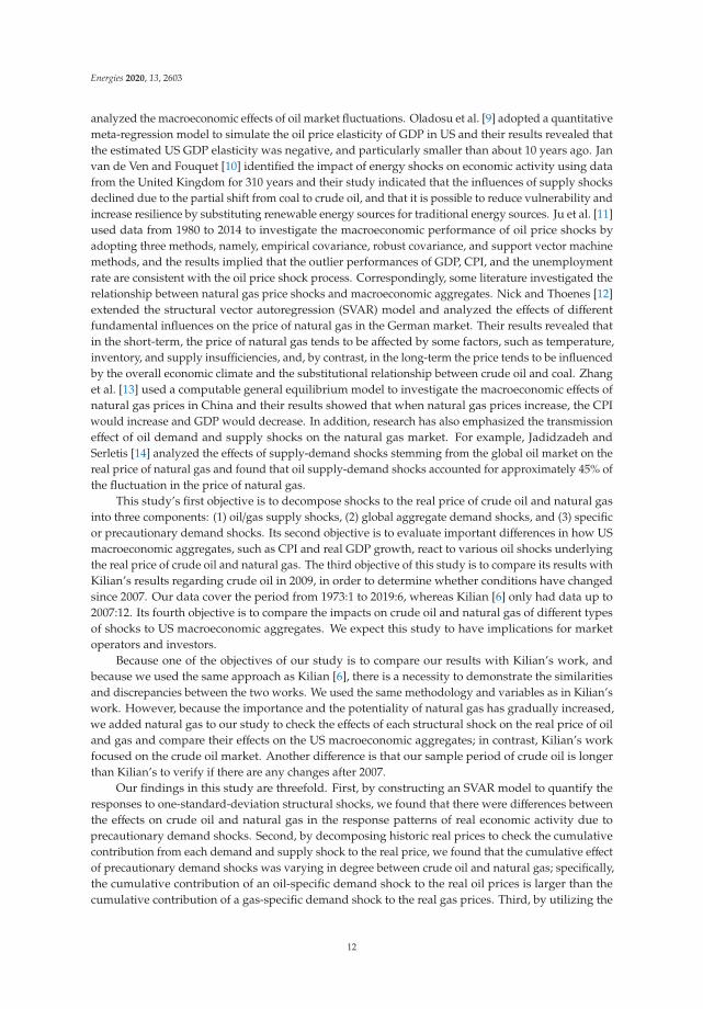
This study’s first objective is to decompose shocks to the real price of crude oil and natural gasinto three components: (1) oil/gas supply shocks, (2) global aggregate demand shocks, and (3) specificor precautionary demand shocks. Its second objective is to evaluate important differences in how USmacroeconomic aggregates, such as CPI and real GDP growth, react to various oil shocks underlyingthe real price of crude oil and natural gas. The third objective of this study is to compare its results withKilian’s results regarding crude oil in 2009, in order to determine whether conditions have changedsince 2007. Our data cover the period from 1973:1 to 2019:6, whereas Kilian [6] only had data up to2007:12. Its fourth objective is to compare the impacts on crude oil and natural gas of different typesof shocks to US macroeconomic aggregates. We expect this study to have implications for marketoperators and investors.

Because one of the objectives of our study is to compare our results with Kilian’s work, andbecause we used the same approach as Kilian [6], there is a necessity to demonstrate the similaritiesand discrepancies between the two works. We used the same methodology and variables as in Kilian’swork. However, because the importance and the potentiality of natural gas has gradually increased,we added natural gas to our study to check the effects of each structural shock on the real price of oiland gas and compare their effects on the US macroeconomic aggregates; in contrast, Kilian’s workfocused on the crude oil market. Another difference is that our sample period of crude oil is longerthan Kilian’s to verify if there are any changes after 2007.

Our findings in this study are threefold. First, by constructing an SVAR model to quantify theresponses to one-standard-deviation structural shocks, we found that there were differences betweenthe effects on crude oil and natural gas in the response patterns of real economic activity due toprecautionary demand shocks. Second, by decomposing historic real prices to check the cumulativecontribution from each demand and supply shock to the real price, we found that the cumulative effectof precautionary demand shocks was varying in degree between crude oil and natural gas; specifically,the cumulative contribution of an oil-specific demand shock to the real oil prices is larger than thecumulative contribution of a gas-specific demand shock to the real gas prices. Third, by utilizing the

12

Energies 2020, 13, 2603

regression model to investigate how oil and gas demand and supply shocks that underlie the realprice of oil and gas influence US macroeconomic aggregates, we found that precautionary demandshocks on crude oil and natural gas have different effects on CPI inflation and had similar effects onreal GDP growth. Both oil- and gas-specific demand shocks led to a small, but statistically insignificant,reduction of the US GDP level. Oil-specific demand shocks tended to cause a large and statisticallysignificant increase in CPI inflation; by contrast, gas market-specific demand shocks led to a small andstatistically insignificant increase in the US CPI level. This result implied policymakers should reactdifferently to gas-specific demand shocks and oil-specific demand shocks.

The remainder of this paper is organized as follows. Section 2 provides a detailed descriptionof the data and introduces the econometric model, a two-stage method based on the SVAR modelproposed by Kilian [6]. Section 3 identifies the structural shocks that drive the real price of crude oiland natural gas. We quantify the historical evolution of these shocks and the response to these shocksfrom production, real activity, and the real price of crude oil and natural gas. We decompose the realprice of crude oil and natural gas over time to assess the respective cumulative contribution of eachshock to real prices. Finally, we analyze the effects of those shocks on US macroeconomic aggregates.Section 4 concludes the study.

2. Materials and Methods

2.1. Data

Table 1 describes the datasets we utilized and their sources. These datasets included crude oilproduction, gas production, a real economic activity index (the Kilian index available on his website),crude oil prices, natural gas prices, and US real GDP, deflated using US CPI (Kilian [6]).

Table 1. Data descriptions and sources.

Variable Sample Period Frequency Description Data Source

Δoprodt 1973:1–2019:6 monthly Percentage change in globalcrude oil production IEA 2

l_reat 1973:1–2019:6 monthly Logarithmic real economicactivity index (Kilian index) Lutz Kilian website [15]

l_rpot 1973:1–2019:6 monthly Log real price of crude oil 1 Federal Reserve Bank

Δgprodt 1994:1–2019:6 monthly Percentage change in globalnatural gas production IEA 2

l_rpgt 1994:1–2019:6 monthly Log real price of natural gas 1 Federal Reserve Bankgdp_gr 1973:1–2019:6 quarterly Real US GDP growth OECD

cpi 1973:1–2019:6 quarterly US CPI OECD1 Real price means price which is deflated by US CPI. 2 Data from the International Energy Agency.

We collected data from Bloomberg, Thomson Reuters, and OECD Stat. These datasets include thecrude oil spot price (West Texas Intermediate, WTI) and the natural gas spot price (Henry Hub). l_rpot

defers to the real price of crude oil expressed in log terms. l_rpgt defers to the real price of natural gasexpressed in log terms. Regarding the dataset of the Kilian index, we collected the data from the LutzKilian website. From Kilian (2009), the Kilian index is a detrended real freight rate index constructedas a measure of monthly global real economic activity, which could imply the variation of worldwidereal economic activity and capture the shifts in the demand for industrial commodities throughoutinternational markets [6,15] (see Appendix A for details). In this study, l_reat defers to the Kilian index;because the minimum of the Kilian index is −161.643, we added 196 to every data point and expressedthe series in log terms. We collected production data for oil and gas from the International EnergyAgency (IEA), and calculated the change rate of oil/gas production in percentage terms to reflect thepercentage change of worldwide oil/gas production. Δoprodt refers to the percentage change in globalcrude oil production, and Δgprodt refers to the percentage change in global natural gas production. US

13

Energies 2020, 13, 2603

real GDP growth and US CPI data was collected from the Organization for Economic Co-operationand Development (OECD); because data for the US real GDP growth rate is unavailable at a monthlyfrequency, we adopted the quarterly frequency when we downloaded the US real GDP growth rateand US CPI datasets. The sample period for crude oil data was from January 1973 to June 2019, but thenatural gas sample was limited by the available data period of January 1994 to June 2019.

The descriptive statistics and stationarity tests for the variables are shown in Table 2. This tableindicates the mean, maximum, minimum, and standard deviation of each variable. (Although the logof the real price of natural gas may have a unit root, we checked the stability condition of the SVARsystem and found that the system is stationary; more details are provided in Appendix B.)

Table 2. The results of unit root tests for the variables.

Δoprodt l_reat l_rpot Δgprodt l_rpgt gdp_gr cpi

Mean 0.00086 5.24667 3.34438 0.00270 1.25432 0.67169 153.274Maximum 0.06714 5.95382 4.84602 0.05266 2.56832 3.86425 255.310Minimum −0.09432 3.53681 1.20789 −0.04827 0.32930 −2.16381 42.7000Std. Dev. 0.01502 0.28056 0.72775 0.01415 0.48039 0.77499 61.5513

Unit root test t-stat. −25.426 −4.356 −2.893 −15.103 −2.473 −9.62668 −10.238Unit root test Prob. 0.000 0.000 0.047 0.000 0.123 0.000 0.000

2.2. Methodology

Based on the two-stage method proposed by Kilian [6], first we identified the structural shocksby estimating the SVAR model and decomposing the structural shocks. Second, we constructed aregression model to investigate how the structural shocks affected US macroeconomic aggregates suchas real GDP growth and CPI inflation. This methodology is widely used in investigations related tooil and natural gas price shocks. For instance, Sim and Zhou [16] applied a structural VAR modeland a quantile regression model to examine the relationship between oil prices and US stock returns.Yoshizaki and Hamori [17] utilized the same model to analyze the reaction of economic activity,inflation, and exchange rates to oil prices shocks. Ahmed and Wadud [18] also used a structural VARmodel to identify the role of oil price shocks on the Malaysian economy and monetary responses.

2.2.1. The SVAR Model

Consider an SVAR model based on a monthly data set for crude oil, ot = (Δoprodt, reat, rpot),where Δoprodt represents the percentage change in global crude oil production, reat represents an indexof real economic activity, and rpot represents the real price of crude oil. In addition, consider an SVARmodel for natural gas, gt = (Δgprodt, reat, rpgt), where Δgprodt represents the percentage change inglobal natural gas production, reat represents an index of real economic activity, and rpgt representsthe real price of natural gas.

Thus, the representation of the SVAR model of crude oil is:

A0ot = α+24∑i

Aiot−i + εt (1)

where εt represents the vector of mutually and serially uncorrelated structural innovations. Althoughthe lag length indicated by Akaike’s information criterion was 14, we decided to use 24, as also usedby Kilian, because we used monthly data series in the model. Using 24 lags avoids the dynamicmisspecification problem [6]. When the error terms are related, they have a common componentthat cannot be recognized by any particular variable, thus, we performed an adjustment to make the

14

Energies 2020, 13, 2603

error terms orthogonal by structural decomposition. We assumed that A−10 has a recursive structure;

therefore, we can decompose the errors et according to et = A−10 εt:

et =

⎛⎜⎜⎜⎜⎜⎜⎜⎜⎝eΔoprod

terea

terpo

t

⎞⎟⎟⎟⎟⎟⎟⎟⎟⎠ =⎡⎢⎢⎢⎢⎢⎢⎢⎢⎣

a11 0 0a21 a22 0a31 a32 a33

⎤⎥⎥⎥⎥⎥⎥⎥⎥⎦⎛⎜⎜⎜⎜⎜⎜⎜⎜⎜⎝

εoil supply shockt

εaggreagate demand shocktε

oil−speci f ic demand shockt

⎞⎟⎟⎟⎟⎟⎟⎟⎟⎟⎠ (2)

Based on Equation (2), we have three structural shocks to be identified, namely an oil supply shock,an aggregate demand shock, and an oil-specific demand shock. As noted by Kilian [6], an oil supplyshock is designed to capture unexpected innovations to international oil output. An aggregate demandshock, which is driven by the global business cycle, is designed to identify the unexpected innovationsto global economic activity. Finally, an oil-specific demand shock, or precautionary demand shock,which is driven by increasing uncertainty in the oil market, is designed to identify the exogenous shiftsin precautionary demand.

It must be noted that, as Equation (2) shows, in the first row of A−10 , the restriction a12 = a13 =

0 implies that innovations to global oil production can only be explained by the oil supply shocks; inthe middle row, the restriction a23 = 0 indicates that innovations to worldwide economic activity canbe explained by oil supply and aggregate demand shocks rather than an oil-specific demand shock.The restriction of the last row shows that all of the three shocks could have effects on the real price ofcrude oil.

Therefore, we can obtain the structural residuals by estimating from Equations (1) and (2). Herewe can plot the structural residuals to observe the changing composition of the structural shocksover time. Then, we can check the dynamic response pattern of the endogenous variables to variousstructural shocks by imposing a one-standard-deviation structural shock.

Similarly, the representation of the SVAR model of natural gas is:

A0gt = β+24∑i

Aigt−i +ωt (3)

We can also decompose the errors wt according to wt = A−10 ωt to identify the structural shocks:

wt =

⎛⎜⎜⎜⎜⎜⎜⎜⎜⎝ω

Δoprodtωrea

tω

rpot

⎞⎟⎟⎟⎟⎟⎟⎟⎟⎠ =⎡⎢⎢⎢⎢⎢⎢⎢⎢⎣

a11 0 0a21 a22 0a31 a32 a33

⎤⎥⎥⎥⎥⎥⎥⎥⎥⎦⎛⎜⎜⎜⎜⎜⎜⎜⎜⎜⎝

ωgas supply shockt

ωaggreagate demand shockt

ωgas−speci f ic demand shockt

⎞⎟⎟⎟⎟⎟⎟⎟⎟⎟⎠ (4)

2.2.2. Regression Model

The purpose of this step is to investigate how the structural shocks estimated from the structuralVAR model in Section 2.2.1 influence the US macroeconomic aggregates, such as CPI inflation (πt) orreal GDP growth (Δyt). The effects are identified by the following regressions:

Δyt = α j +12∑

i=0

φ jiζ jt−i + ujt (5)

πt = δ j +12∑

i=0

ψ jiζ jt−i + vjt (6)

ζojt =

13

3∑i=1

ε j,t,i, j = 1, 2, 3 (7)

15

Energies 2020, 13, 2603

ζgjt =

13

3∑i=1

ω j,t,i, j = 1, 2, 3 (8)

In this regression model, ujt and vjt refer to errors; φ ji and ψ ji represent the impulse responsecoefficients, respectively; ε j,t,i denotes the estimated residual for the jth structural shock in the ithmonth of the tth quarter in the crude oil data; and ω j,t,i denotes the estimated residual for the jthstructural shock in the ith month of the tth quarter in the natural gas data. Furthermore, we determinedthe number of lags to be 12 quarters as also used by Kilian [6].

3. Results

3.1. Identifying Structural Shocks

Figures 1–4 summarize the empirical results of the SVAR model based on Equations (1)–(4) fromSection 2. After obtaining the model estimates, we can calculate the structural residuals.

3.1.1. Quantifying the Evolution of Crude Oil and Natural Gas Demand and Supply Shocks

Figure 1 plots the time path of the structural shocks estimated by the model.Figure 1 reveals that, at any point in time, the real price of crude oil was reacting to multiple

shocks, the combination of which evolved:

• In 2008, the oil side results were characterized by a sharp plummet due to the global aggregatedemand shock associated with the 2008 financial crisis. In 2008, the oil-specific structuraldemand shock also led to a sharp fall associated with the dramatic increase in the price of crudeoil. Accordingly, the demand for natural gas increased, leading to a substantial and positivegas-specific structural demand shock.

• One point to note is that because the time periods for the crude oil and natural gas structuralshocks did not overlap, it is inappropriate to conclude that the amplitude and frequency of crudeoil structural shocks were greater than those of natural gas structural shocks.

(oil) oil supply shock

(oil) aggregate demand shock

Figure 1. Cont.

16

Energies 2020, 13, 2603

(oil) oil specific demand shock

(gas) gas supply shock

(gas) aggregate demand shock

(gas) gas specific demand shock

Figure 1. Historical evolution of structural shocks. From top to bottom, column (oil) illustrates crudeoil supply, aggregate demand, and oil-specific demand shocks from 1976 to 2019. From top to bottom,column (gas) illustrates natural gas supply, aggregate demand, and gas-specific demand shocks from1996 to 2019. Note: Structural residuals implied by Equations (1)–(4), averaged annually.

3.1.2. Responses to One-Standard-Deviation Structural Shocks

Figure 2 plots the responses of global oil and gas production, real economic activity, and the realprice of oil and gas to a one-standard-deviation structural innovation.

Figure 2 reveals how global oil and gas production, real economic activity, and the real priceof oil and gas responded to demand and supply shocks, respectively, in the crude oil and naturalgas markets.

First, the empirical results for crude oil are as follows: Concerning oil supply shocks, we caninterpret from the graph that positive oil supply shocks, in which production rose, caused a sharpincrease, followed by a reversal of the increase to its initial level within the first quarter. At the same

17

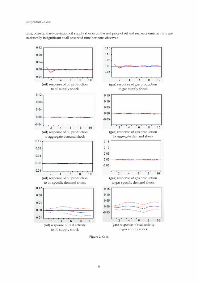
Energies 2020, 13, 2603

time, one-standard-deviation oil supply shocks on the real price of oil and real economic activity arestatistically insignificant at all observed time horizons observed.

(oil) response of oil production

to oil supply shock

(gas) response of gas production

to gas supply shock


to aggregate demand shock




to oil specific demand shock


to gas specific demand shock

(oil) response of real activity

to oil supply shock

(gas) response of real activity

to gas supply shock

Figure 2. Cont.

18

Energies 2020, 13, 2603

(oil) response of real activity to aggregated demand shock

(gas) response of real activity to aggregated demand shock

(oil) response of real activity to oil specific demand shock

(gas) response of real activity to gas specific demand shock

(oil) response of real price of oil

to oil supply shock

(gas) response of real price of gas

to gas supply shock


to aggregated demand shock


to aggregated demand shock





Figure 2. Responses to one-standard-deviation structural shocks. From top to bottom, the first columnin (oil) illustrates the responses of crude oil production, real economic activity, and the real price of oil,to oil supply shocks, aggregate demand shock, and oil-specific demand shock, respectively. From topto bottom, the second column in (gas) illustrates the responses of natural gas production, real economicactivity, and real price of gas to gas supply shocks, aggregate demand shock, and gas-specific demandshock, respectively. Note: Estimates based on Equations (1)–(4).

19

Energies 2020, 13, 2603

(oil) cumulative effect of oil supply shock

on real price of oil

(gas) cumulative effect of gas supply shock

on real price of gas

(oil) cumulative effect of aggregate demand

shock on real price of oil

(gas) cumulative effect of aggregate demand

shock on real price of gas

(oil) cumulative effect of oil specific demand

shock on real price of oil

(gas) cumulative effect of gas specific demand

shock on real price of gas

Figure 3. Historical decomposition of the real prices of crude oil and natural gas. From top to bottom,(oil) illustrates the cumulative effect of oil supply, aggregate demand, and oil market-specific demandshocks on the real price of crude oil. From top to bottom, (gas) illustrates the cumulative effect of gassupply, aggregate demand, and gas market-specific demand shocks on the real price of natural gas.Note: Estimates derived from Equations (1)–(4).

Regarding the effect of an aggregate demand expansion on real global economic activity, we caninterpret from the graph that a positive aggregate demand shock caused a transitory but substantialincrease that reached its maximum in period 2, followed by a gradual decline until the 8th month, andan increase again after 9 months. At the same time, a one-standard-deviation aggregate demand shockcaused a very stable and statistically significant increase in the real price of oil.

The series of graphs showing the “(oil) response to an oil-specific demand shock” reveal thatoil-specific demand increases had an immediate, large, persistent, and positive effect on the real priceof crude oil in the first 2 months, which thereafter gradually declined but remained positive and highlystatistically significant. At the same time, these shocks also triggered a statistically significant increasein real economic activity in the first 3 months, followed by a decrease that remained statisticallysignificant until the 9th month. This compares to the results from Kilian [6], in which the statisticalsignificance lasted until the 12th month. Regarding this difference, we estimate that the influence ofspecific demand shocks on global economic activity is shorter than it was before 2009, which providesevidence for the phenomenon that, as the new economic environment changes rapidly, the economiccycle shortens.

To summarize the crude oil results, aggregate demand shocks had a positive effect on both realglobal economic activity and the real price of crude oil. Precautionary demand shocks caused arelatively longer and positive effect on the real price of oil, and led to small, transitory increases in realeconomic activity. These results are generally the same as those reported by Kilian [6], except thatKilian’s work showed that oil supply shocks caused a partially statistically significant and small declinein the real price of oil, and caused an extremely small increase in real economic activity, while our resultsshowed that the shocks on the real price and the real economic activity are statistically insignificant.

20

Energies 2020, 13, 2603

(oil) cumulated response of US real GDP

to oil supply shock

(gas) cumulated response of US real GDP

to gas supply shock









(oil) cumulated response of US CPI level to

oil supply shock

(gas) cumulated response of US CPI level to

gas supply shock


aggregate demand shock


aggregate demand shock


oil specific demand shock


gas specific demand shock

Figure 4. The responses of US real GDP growth and CPI inflation to each structural shock. Note: Theplots show the cumulative responses, as estimated from the regression models.

Second, the empirical results of natural gas are as follows: Concerning natural gas supply shocks,positive supply shocks where production rose caused small but sharp increases, followed by a returnto its initial level within the first quarter. At the same time, a one-standard-deviation natural gassupply shock caused a partially statistically significant decline in the real price of natural gas in thefirst 3 months, and caused a negligible increase in real economic activity.

21

Energies 2020, 13, 2603

Regarding the effect of an aggregate demand expansion on real global economic activity, wecan interpret from the graph that a positive aggregate demand shock caused a transitory and highlysignificant increase that reached its maximum level in the 2nd month, followed by a gradual declineuntil the 8th month, and an increase again after 9 months. This result is similar to the result of the crudeoil model. Aggregate demand shocks also caused a very stable and statistically significant increase inthe real price of natural gas.

The last natural gas graph reveals that gas-specific demand increases have an immediate, noticeable,stable, and statistically significant positive effect on the real price of natural gas that gradually declinesafter the 3rd month but remains positive. At the same time, these shocks also triggered extremely smallincreases in real economic activity, followed by declines and then small increases that were statisticallyinsignificant by the 10th month. This result suggests that precautionary demand shocks to natural gashardly affected real economic activity.

To summarize the natural gas results, aggregate demand shocks had a positive effect on real globaleconomic activity and the real price of natural gas. Precautionary demand shocks caused a relativelyshorter, positive effect on the real price of natural gas.

Comparing the results between crude oil and natural gas reveals that they are similar, with minordifferences. The major distinction relates to the different effects on real economic activity that resultfrom precautionary demand shocks to crude oil versus natural gas.

3.1.3. The Cumulative Effect of Oil and Gas Demand and Supply Shocks on the Real Prices of Oiland Gas

According to the results of a historical decomposition of the data sets, the respective cumulativecontributions of demand and supply shocks to the real prices of crude oil and natural gas are plottedin Figure 3.

Figure 3 reveals the respective cumulative contributions of oil and gas demand and supply shocksto the real prices of oil and gas.

First, the empirical results for crude oil are as follows: The top graph implies that real oil supplyshocks have historically made relatively small contributions to the real price of crude oil. The biggestcontributions have been oil market-specific demand shocks. While aggregate demand shocks led tolong swings in real global economic activity, oil market-specific demand shocks were the primaryreasons for relatively sharp and defined increases or decreases in the real price of oil. This resultis consistent with the results investigated above, and provides further evidence for the propositionthat precautionary demand shocks cause relatively immediate increases in real prices. Furthermore,the shocks cause relatively small but stable increases in real economic activity.

To summarize these results for crude oil, precautionary demand shocks made the greatestcontributions to the real price of oil. Our results for crude oil are approximately similar to Kilian [6],but one concern is that, during the period 1985–2000, Kilian’s study showed a negative cumulativeeffect of an aggregate demand shock on the real price of crude oil, while the effect in our study wasextremely close to zero.

Second, the empirical results for natural gas are as follows: The first graph shows that real gassupply shocks have historically made relatively small contributions to the real price of natural gas.The largest contributions were due to global aggregate demand shocks and specific demand shocksin the oil market. However, aggregate demand shocks displayed a long-term and relatively smoothmovement in the real price of natural gas. In contrast, gas market-specific demand shocks accountedfor the sharply defined increases and decreases. This result implies the same suggestion that wealready stated above regarding crude oil.

To summarize the natural gas results, the cumulative contribution of precautionary and aggregatedemand shocks accounted for a large proportion of the real price of natural gas. From these empiricalresults for natural gas, attention should be paid to the fact that, during the years of financial crises in1998 and 2008, the degree of the cumulative effect of the precautionary demand shocks was different;

22

Energies 2020, 13, 2603

specifically, the cumulative contribution of the oil-specific demand shock to the real price of oil is largerthan the cumulative contribution of the gas-specific demand shock to the real price of gas. This issueremains open for investigation in the future.

Comparing these two results, the major difference between oil and gas was the cumulative effectof precautionary demand shocks on their real prices.

3.2. Effects on the US Economy

Based on estimations from Equations (5)–(8), Figure 4 plots the responses of US real GDP and CPIto each of the three shocks defined previously.

The results in Figure 4 reveal important differences in how oil and gas demand and supply shocksthat underlie the real prices of oil and gas affect US macroeconomic aggregates such as US real GDPgrowth and CPI inflation.

First, the empirical results for crude oil are as follows: The graphs of the (oil)-cumulative responseof US real GDP/CPI levels to an oil supply shock imply that oil supply shocks created a partiallystatistically significant decrease in US real GDP from its initial level and a rise in the 3rd year. Theeffect on US real GDP was negative for all 16 quarters; however, the two standard error bands werestatistically significant for only half a year, compared to the two years reported in Kilian [6]. In contrast,the corresponding effects on the CPI level were mostly statistically insignificant, and displayed adeclining tendency.

The graphs of the (oil)-cumulated response of the US real GDP/CPI levels to an aggregate demandshock indicate that unanticipated aggregate demand shocks increased US real GDP statisticallysignificantly in the first year, and then caused the GDP level to decline below its initial level in the2nd year, with the decrease becoming statistically significant again after the 3rd year. In contrast, thecorresponding effects on the level of CPI indicated a persistent, gradual increase that was statisticallysignificant at all time horizons observed, whereas in Kilian’s results it became statistically significantonly after the 3rd quarter [6].

Finally, unanticipated oil-specific demand shocks lowered US real GDP gradually, and thereduction was statistically insignificant at all observed time horizons. In contrast with this result,Kilian [6] showed that the decline reached its maximum in the 3rd year, and implied statisticalsignificance in the 3rd year of under one standard error band. It should be noted that Kilian’s resultswere also statistically insignificant under two standard error bands. Meanwhile, these shocks led to asustained, gradual, and statistically significant increase in the US CPI level, which is consistent withKilian’s results [6].

To summarize the results for crude oil, our first result was that oil supply shocks led to transitoryreductions in the US real GDP level, and barely affected the CPI level. Second, aggregate demandshocks had positive effects on US GDP growth during the first year and stimulated immediate increasesin the CPI level, which is a different result from Kilian [6]. Kilian found that aggregate demand shockscaused delays in the rise of the CPI level for 3 quarters. Third, oil-specific demand shocks led toincreases in the CPI inflation level and barely affected the US real GDP level.

Second, the empirical results for natural gas are as follows: The graphs of the (gas)-cumulativeresponse of US real GDP/CPI level to a gas supply shock imply that the responses of the US real GDPand CPI levels to gas supply shocks are relatively small and statistically insignificant.

The graphs of the (gas)-cumulative response of US real GDP/CPI levels to an aggregate demandshock reveal that unanticipated aggregate demand shocks caused extremely small, statisticallyinsignificant increases in the US real GDP level within 2 quarters, and then caused the real GDP levelto decline below its initial level after the 3rd quarter, with the decrease becoming partially statisticallysignificant after the 3rd year. In contrast, the corresponding effect on the level of CPI showed asustained, gradual increase, and was statistically significant for all 16 quarters.

The graphs of the (gas)-cumulative response of US real GDP/CPI levels to a gas-specific demandshock indicate that unanticipated gas-specific demand shocks reduced the US real GDP level gradually,

23

Energies 2020, 13, 2603

slightly, and statistically insignificantly. In contrast, these shocks led to sustained, gradual, butstatistically insignificant increases in the US CPI level.

To summarize the results for natural gas, our first result was that gas supply shocks barely affectedthe level of US real GDP or CPI. Second, aggregate demand shocks caused a gradual decline in US realGDP growth that was partially statistically significant, but stimulated an immediate and statisticallysignificant increase in the CPI level. Third, gas-specific demand shocks hardly affected the US realGDP and CPI inflation levels.

To compare these two results, the major difference was that precautionary demand shocks in crudeoil and natural gas had different effects on CPI inflation. Oil market-specific demand shocks tendedto statistically significantly increase the CPI inflation level greatly; in contrast, gas market-specificdemand shocks led to a small and statistically insignificant increase in the CPI inflation level. Anotherpoint is that aggregate demand shocks in the oil market increase and then lower the US real GDP levelsignificantly for the most part, whereas aggregate demand shocks in the gas market led to insignificantdecreases in the US real GDP level for the most part.

4. Conclusions

This paper investigated the response of US macroeconomic aggregates to price shocks in crude oiland natural gas markets using a two-step approach: firstly decomposing the price shocks to identifythe structural shocks using a structural VAR model, and secondly, showing the response patterns ofmacroeconomic aggregates corresponding to each structural shock using a regression model.

Our main findings in this study are threefold. First, we found that there was a difference in theeffects on real economic activity due to precautionary demand shocks from crude oil versus naturalgas. Second, the cumulative contribution of oil-specific demand shocks to real oil prices is larger thanthe cumulative contribution of gas-specific demand shocks to real gas prices. Third, precautionarydemand shocks had different effects on CPI inflation, depending on whether they were due to crudeoil or natural gas. Therefore, economists, policymakers, and investors must decompose real prices ofthese important energy sources that have such significance in the economy and our daily lives. Finally,the most noteworthy of our findings is that oil market-specific demand shocks lead to statisticallysignificant increases in the US CPI level, however, gas market-specific demand shocks barely affect theUS CPI level. This result implies policymakers should react differently to gas-specific demand shocksand oil-specific demand shocks.

The similarities and differences between our empirical results and those of Kilian [6] can besummarized as follows. Firstly, comparing the results which showed the responses of global oil/gasproduction, real economic activity, and the real price of oil/gas to structural innovation reveal thatthey are alike with minor differences. The major distinction is the different effects on real economicactivity that result from precautionary demand shocks to crude oil versus natural gas. Another point isthat the statistically significant lasting period of influence from oil-specific demand shocks on globaleconomic activity were shorter than they were prior to 2009, as the results from Kilian [6] showed.Secondly, comparing the results of the historical decomposition of real prices, our results for crudeoil are approximately similar to Kilian, but one concern is that, during the period 1985–2000, Kilian’sstudy showed a negative cumulative effect of an aggregate demand shock on the real price of crudeoil, while the effect in our study was extremely close to zero [6]. Thirdly, comparing the result ofeffects of respective shocks on the US macroeconomy, the empirical results are very similar with minordifferences. The results of oil supply shocks on GDP showed that the two standard error bands werestatistically significant for only half a year, compared to the two years reported in Kilian [6], which wasexplained by the one standard error band. Because of the different adoption of the standard error band,unanticipated oil-specific demand shocks led to a statistically insignificant reduction in US real GDP forall observed time horizons, whereas Kilian’s results implied statistical significance in the 3rd year [6].

Compared to previous literature, namely Zhang et al. (2017) [13], the similarities and discrepanciesshould be noted. Because not all natural gas price shocks cause GDP to decrease and the CPI to

24

Energies 2020, 13, 2603

increase, when natural gas price increases originate from increasing uncertainty of the energy market,GDP would decline, and the CPI would rise. However, when natural gas price shocks are due toexogenous supply shocks, GDP would not always decrease, while the CPI would decline, which is adifferent outcome from that relating to aggregate shocks and specific demand shocks.

In this paper, the empirical evidence may have some implications for economists, policymakers,and investors albeit their self-evidence. Because our empirical results showed that the response patternsvary depending on the causes of the price fluctuations, not only for the crude oil market, but alsothe natural gas market, economists should take this into account when they construct their modelsfor researching about oil/gas price shocks. Regarding the policy-making implications, especially forgovernment monetary authorities such as central banks, there is a need to identify the underlyingdeterminants that drive the price increases to make appropriate policy. For example, when the oil orgas price increase stems from an exogenous supply shock, there is almost no need to undertake anycountermeasures because these kinds of shocks have a minimal effect on the macroeconomic aggregates.In contrast, with supply shocks, in which the price increases because of surging uncertainty in theoil market, thereby stimulating an increase in precautionary demand, monetary authorities shouldconsider whether countermeasures should be undertaken to retard ongoing inflation; there is almostno need to take such countermeasures into account in the case of the gas market. Another implicationconcerns aggregate demand shocks: policymakers should distinguish where the aggregate demandshocks originated i.e., the crude oil market or the natural gas market. If the source of the shock lies inthe oil market rather than the gas market, the corresponding responses should take into considerationprevention of a reduction of the GDP level over the long-run. As for the long-term investmentimplications, firstly, the investors must distinguish the origins of the oil/gas price fluctuation becausethe response pattern of each shock is different and requires distinct investment adjustments. Secondly,investors should pay attention to global aggregate demand shocks, and the specific demand shockrather than supply shocks, when they reconsider their investment structure, because precautionarydemands shocks make a greater contribution to real price fluctuations than exogenous supply shocks.Because of developing environmental awareness, the demand for natural gas is gradually increasingand growing in importance in energy markets, thus implying that investors should take natural gasas an alternative investment choice for their portfolio adjustment when turbulence occurs in crudeoil markets.

Despite our findings, this investigation has several limitations. First, the range of the datasetof natural gas prices is from 1994, which makes it impossible to compare the cumulative effect ofdemand and supply shocks between crude oil and natural gas during the period 1973–1993. Second,we adopted the Kilian Index (Kilian [6]); however, whether the Kilian Index is an adequate reflectionof overall economic activity after 2009 is beyond the scope of this study. Because the driving forcesand factors which influence global economic activity may have changed after 2009, there may now bea more appropriate index. Third, as mentioned above, during the period 1985–2000, Kilian’s studyshowed a negative cumulative effect of an aggregate demand shock on the real price of crude oil, whilethe effect in our study was extremely close to zero. The proper explanation for this outcome remainsunknown and requires further research.

Therefore, in our future research, first, we plan to identify a more appropriate index to reflectoverall global economic activity, and compare the results with those based on the Kilian Index. Second,as noted in Section 3.1.3, the cumulative contribution of an oil-specific demand shock to real prices islarger than the cumulative contribution of a gas-specific demand shock. Thus, we intend to identifythe underlying determinants or causes of this issue. Third, in order to effectively apply our resultsto the policy-making process and inform appropriate monetary policy, we propose to extend theresults by a machine learning approach to forecast price fluctuations corresponding to various kinds ofuncertainty conditions, namely financial crises, wars, emergencies, disasters, etc. Fourth, the approachof Kilian [6], followed herein, did not include analysis of cointegration; thus, we plan to expand theanalysis within the framework of cointegration. Finally, assessing the effects of oil/gas price shocks on

25

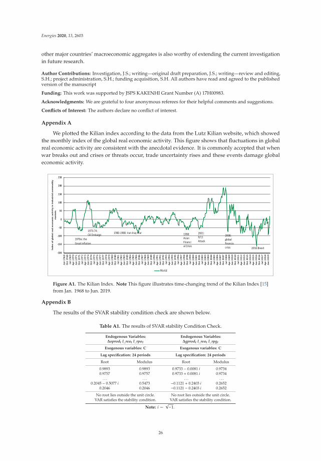
Energies 2020, 13, 2603

other major countries’ macroeconomic aggregates is also worthy of extending the current investigationin future research.

Author Contributions: Investigation, J.S.; writing—original draft preparation, J.S.; writing—review and editing,S.H.; project administration, S.H.; funding acquisition, S.H. All authors have read and agreed to the publishedversion of the manuscript

Funding: This work was supported by JSPS KAKENHI Grant Number (A) 17H00983.

Acknowledgments: We are grateful to four anonymous referees for their helpful comments and suggestions.

Conflicts of Interest: The authors declare no conflict of interest.

Appendix A

We plotted the Kilian index according to the data from the Lutz Kilian website, which showedthe monthly index of the global real economic activity. This figure shows that fluctuations in globalreal economic activity are consistent with the anecdotal evidence. It is commonly accepted that whenwar breaks out and crises or threats occur, trade uncertainty rises and these events damage globaleconomic activity.

Figure A1. The Kilian Index. Note This figure illustrates time-changing trend of the Kilian Index [15]from Jan. 1968 to Jun. 2019.

Appendix B

The results of the SVAR stability condition check are shown below.

Table A1. The results of SVAR stability Condition Check.

Endogenous Variables:Δoprodt l_reat l_rpot

Endogenous Variables:Δgprodt l_reat l_rpgt

Exogenous variables: C Exogenous variables: C

Lag specification: 24 periods Lag specification: 24 periods

Root Modulus Root Modulus

0.9893 0.9893 0.9733 − 0.0081 i 0.97340.9757 0.9757 0.9733 + 0.0081 i 0.9734. . . . . . . . . . . .

0.2045 − 0.5077 i 0.5473 −0.1121 + 0.2403 i 0.26520.2046 0.2046 −0.1121 − 0.2403 i 0.2652

No root lies outside the unit circle. No root lies outside the unit circle.VAR satisfies the stability condition. VAR satisfies the stability condition.

Note: i =√−1.

26

Energies 2020, 13, 2603

References

1. International Energy Agency. World Energy Outlook 2019. 2019. Available online: https://www.iea.org/weo/(accessed on 3 May 2020).

2. International Energy Agency. Gas-Fuels &Technologies. Available online: https://www.iea.org/fuels-and-technologies/gas (accessed on 3 May 2020).

3. Hamilton, J.D. Oil and the Macroeconomy since World War II. J. Political Econ. 1983, 91, 228–248. [CrossRef]4. Hamilton, J.D. This is what happened to the oil price-macroeconomy relationship. J. Monet. Econ. 1996, 38,

215–220. [CrossRef]5. Hooker, M.A. What happened to the oil price-macroeconomy relationship? J. Monet. Econ. 1996, 38, 195–213.

[CrossRef]6. Kilian, L. Not all oil price shocks are alike: Disentangling demand and supply shocks in the crude oil market.

Am. Econ. Rev. 2009, 99, 1053–1069. [CrossRef]7. Kling, J.L. Oil price shocks and stock-market behavior. J. Portf. Manag. 1985, 12, 34–39. [CrossRef]8. Kilian, L.; Park, C. The impact of oil price shocks on the U.S. stock market. Int. Econ. Rev. 2009, 50, 1267–1287.

[CrossRef]9. Oladosu, G.A.; Leiby, P.N.; Bowman, D.C.; Uría-Martínez, R.; Johnson, M.M. Impacts of oil price shocks on

the United States economy: A meta-analysis of the oil price elasticity of GDP for net oil-importing economies.Energy Policy 2018, 115, 523–544. [CrossRef]

10. Jan van de Ven, D.; Fouquet, R. Historical energy price shocks and their changing effects on the economy.Energy Econ. 2017, 62, 204–216. [CrossRef]

11. Ju, K.; Su, B.; Zhou, D.; Wu, J.; Liu, L. Macroeconomic performance of oil price shocks: Outlier evidence fromnineteen major oil-related countries/regions. Energy Econ. 2016, 60, 325–332. [CrossRef]

12. Nick, S.; Thoenes, S. What drives natural gas prices?—A structural VAR approach. Energy Econ. 2014, 45,517–527. [CrossRef]

13. Zhang, W.; Yang, J.; Zhang, Z.; Shackman, J. Natural gas price effects in China based on the CGE model.J. Clean. Prod. 2017, 147, 497–505. [CrossRef]

14. Jadidzadeh, A.; Serletis, A. How does the U.S. natural gas market react to demand and supply shocks in thecrude oil market? Energy Econ. 2017, 63, 66–74. [CrossRef]

15. Kilian Index. Lutz Kilian Homepage. Available online: https://sites.google.com/site/lkilian2019/research/data-sets (accessed on 3 May 2020).

16. Sim, N.; Zhou, H. Oil prices, US stock return, and the dependence between their quantiles. J. Bank. Financ.2015, 55, 1–8. [CrossRef]

17. Yoshizaki, Y.; Hamori, S. On the influence of oil price shocks on economic activity, inflation, and exchangerates. Int. J. Financ. Res. 2013, 4, 33–41. [CrossRef]

18. Ahmed, H.J.A.; Wadud, I.K.M.M. Role of oil price shocks on macroeconomic activities: An SVAR approachto the Malaysian economy and monetary responses. Energy Policy 2011, 39, 8062–8069. [CrossRef]

© 2020 by the authors. Licensee MDPI, Basel, Switzerland. This article is an open accessarticle distributed under the terms and conditions of the Creative Commons Attribution(CC BY) license (http://creativecommons.org/licenses/by/4.0/).

27

energies

Article

Forecasting Crude Oil Market Crashes Using MachineLearning Technologies

Yulian Zhang and Shigeyuki Hamori *

Graduate School of Economics, Kobe University, 2-1, Rokkodai, Nada-Ku, Kobe 657-8501, Japan;[email protected]* Correspondence: [email protected]


Abstract: To the best of our knowledge, this study provides new insight into the forecasting of crudeoil futures price crashes in America, employing a moving window. One is the fixed-length windowand the other is the expanding-length window, which has never been reported in the past. We aimedto investigate if there is any difference when historical data are discarded. As the explanatoryvariables, we adapted 13 variables to obtain two datasets, 16 explanatory variables for Dataset1 and121 explanatory variables for Dataset2. We try to observe results from the different-sized sets ofexplanatory variables. Specifically, we leverage the merits of a series of machine learning techniques,which include random forests, logistic regression, support vector machines, and extreme gradientboosting (XGBoost). Finally, we employ the evaluation metrics that are broadly used to assess thediscriminatory power of imbalanced datasets. Our results indicate that we should occasionally discarddistant historical data, and that XGBoost outperforms the other employed approaches, achieving adetection rate as high as 86% using the fixed-length moving window for Dataset2.

Keywords: oil futures prices crashes; foresting; random forests; logistical regression; support vectormachines; extreme gradient boosting; moving window

1. Introduction

The consumption of energy commodities is becoming a crucial issue, along with modernizationand technological development. Crude oil plays a pivotal role in economic growth as a major energysource. The share of America’s crude oil consumption is as high as 37%, which shows the crucialposition held by crude oil as a component of the energy sources [1]. For energy investors, forecastingoil price crashes can help them mitigate risk and ensure proper resource investment and allocation.Saggu and Anukoonwattaka indicate that economic growth is at significant risk from commodityprice crashes across Asia-Pacific’s least developed countries and landlocked developing countries [2].Research has indicated that a crisis starts from a single economy of a large enough size and generatesturbulence in other countries [3].

The beginning of a recession manifests itself through asset price drops in G-7 countries [4]. The EUallowances price drop can be justified by an economic recession [5]. By forecasting oil price crashes,we can infer recessions and develop an early warning system (EWS) for policymakers, and they canperform relevant actions to curtail the contagion crisis, or preempt an economic crisis or recession.The financial crisis of 2008 rekindled interest in EWSs. An EWS can help policymakers manageeconomic complexity and take precautionary actions to lower risks that can cause a crisis. An EWS canhelp reduce economic losses by providing information that allows individuals and communities toprotect their property.

Many studies have been conducted on crude oil price forecasting [6–8]. Investigations have beenconducted on oil price prediction using machine learning, along with the development and application


Energies 2020, 13, 2440

of machine learning and deep learning [9–14]. However, what we want to know is whether there willbe a huge drop in crude oil futures prices, rather than the specific numbers. Crash and crisis forecastingare significant and may be flexibly applied to finance, banking, business, and other fields. This iswhy crisis prediction and financial contagion have become popular topics in academic investigationin recent years, especially after the global crisis of 2008, which had a significant impact on variousindustries and countries. Studies in the past have provided important information on predictingfinancial crises [3,15] by applying machine learning. Nevertheless, there are still few studies predictingoil futures price crashes. Additionally, we want to fill the gap of crude oil futures price crash forecastingin the crude oil market. Oil price crash forecasting can give the early warning information to investorsand policymakers, so they can do some precautionary action to reduce the loss.

We define the crisis based on [3,15]. Our investigation contributes to the current literature byanalyzing the predictive performance of a series of state-of-the-art statistical machine learning methods,including random forest, logistic regression, support vector machine, and extreme gradient boosting(XGBoost) algorithms, in the classification problem of crude oil futures price market crash detection inAmerica, covering the period from 1990 to 2019. To the best of our knowledge, this study provides newinsights into forecasting oil price crashes, employing a moving window that has never been reportedin the past. Furthermore, we also consider the previous data in the moving window algorithm, and theexperimental work presented here provides a novel result that discarding previous data can achievebetter performance. We develop an exhaustive experimental performance evaluation of our algorithmsusing a test dataset of the daily returns performance of the 25-year oil price market.

Finally, we find that the fixed-length window provides a better result than the expanding window,which indicates that we should occasionally abandon distant historical data, and XGBoost outperformsthe other techniques in this study, achieving a detection rate as high as 86% using the fixed-lengthmoving window for Dataset2.

The remainder of this paper is organized as follows. Section 2 reviews the previous literaturerelated to this study. We provide a brief explanation of the machine learning algorithms and the movingwindow utilized in Section 3. In Section 4, we elaborate on the dataset implemented to perform thesystem. In Section 5, we present an experimental evaluation and provide empirical results. We evaluatethe empirical findings based on a series of assessments, computed on a test dataset sample spanning along period. Finally, we present some concluding remarks in Section 6.


The topic of oil price forecasting has been extensively studied [6–8]. High- and low-inventoryvariables have been used to forecast short-run crude oil prices [16]. The results show that globalnon-oil industrial commodity prices are the most successful predictors of oil prices [6]. Moshiri andForoutan [17] developed a nonlinear model to forecast crude oil futures prices.

With the development of machine learning and deep learning, an increasing number of academicstudies have attempted to research this problem using a machine learning algorithm [9–13]. Wen et al. [9]make crude oil price forecasting based on support vector machines. An empirical model decompositionbased neural network ensemble learning paradigm is proposed for oil spot price forecasting [10].An improved oil price forecast model that uses a support vector machine was developed [18]. Someresearchers forecast the crude oil price using machine learning [12] and the deep learning ensembleapproach [14]. Other researchers use XGBoost [13] and wavelet decomposition and neural networkmodel [11] to forecast crude oil prices. However, compared with the specific figures of crude oil prices,investors and practitioners are more concerned about the drops or crashes of crude oil prices.

An analytic network process model is applied in forecasting the crisis [19]. There are manypapers on predicting financial crises [3,15,20] that apply machine learning. Lean et al. [20] employthe general regression neural networks to predict the currency crisis upon the disastrous 1997–1998currency crisis experience. Based on a multinomial logit model, Bussiere and Fratzscher [15] developa new EWS model to forecast financial crises. Chatzis et al. [3] use deep and statistical machine

30

Energies 2020, 13, 2440

learning techniques (classification trees, support vector machines, random forests, neural networks,extreme gradient boosting, and deep neural networks) to predict stock market crisis events. They findthat forecasting accuracy can be improved by adding oil variables to the traditional predictors ofexcess stock returns of the S&P 500 index. However, investigations into oil price crashes are still veryinadequate. The experimental work presented here provides one of the first investigations into how toforecast crashes of crude oil future prices using machine learning.

Chatzis et al. [3] detect a crisis event based on the number of stock market negative coexceedances(less than 1% percentile of the empirical distribution). Due to the imbalanced dataset, and becausewe want to obtain more crash events, we consider crash events in less than 2.5% percentile of theempirical distribution [15].

A new EWS model for predicting financial crises was developed based on a multinomial logitmodel in [15], and the model correctly predicts the majority of crises in emerging markets. The 2008financial crisis brought huge losses to the financial industry, as well as society as a whole, and peoplegained renewed awareness of the importance of an EWS. Davis and Karim [21] assess and suggest thatthe logit is the most beneficial approach to a global EWS, along with signal extraction for country-specificEWS for banking crises on a comprehensive common dataset. Babecky et al. [22] account for modeluncertainty using Bayesian model averaging, identifying early warning indicators of crises specificto developed economies. The study indicates that the dynamic Bayesian network models can offerprecise early-warnings compared with the logit and signal-extraction methods [23].

Studies on EWSs for financial crises employing machine learning techniques are still limited.This paper develops an EWS that includes artificial neural networks, decision trees, and a logisticregression model [24]. Geng et al. [25] use data mining techniques to build financial distress warningmodels and find that the performance of neural networks is better than decision trees, support vectormachines, and multiple classifiers. Finally, a total of six deep and statistical machine learning techniquesare used to develop the EWS and forecast a stock market crisis [3].

In this paper, we performed the forecasting model using random forests (hereafter RF) [26],logistical regression (hereafter LogR) [27], support vector machines (hereafter SVMs) [28], and extremegradient boosting (hereafter XGBoost). RF is applied in gene expression analysis [29], protein–proteininteractions [30], risk assessment [31], and image classification [32], among others. Ohlson [27] usesLogR for the first time to predict corporate bankruptcy based on financial statement data. LogR andNN (neural networks) are employed to predict the bond rating [33]. SVMs are widely used in creditrating systems in many investigations [34,35]. XGBoost is an important and efficient implementationof the gradient boosting framework in the classification methodology of [36,37].

In terms of oil price crashes forecasting, there are many methods that can be employed.It includes nearest neighbors [38], NN (neural network), which is broadly applied in credit ratingclassification [39,40], and LSTM (long short-term memory), it is employed in forecasting the volatility ofstock price index [41]. In the future, in addition to adding other methods, we can also consider improvethe existing approach. Zhong and Enke [42] use the nature dimensionality reduction technique,means principal component analysis (PCA), and the artificial neural networks (ANNs), yieldingimproved outcomes.

3. Model Development

We utilized the following models: RF [26], LogR [27], SVMs [28], and XGBoost. Then, we presenteda detailed interpretation of the development and parameter tuning of each machine learningmethodological framework.

We used the machine learning models above, and we also considered two patterns of movingwindow corresponding to Section 4, aimed to investigate if there is any difference when historical dataare discarded. One is the fixed-length window and the other is the expanding window.

In terms of the fixed-length window, for daily data, we considered 1000 days (almost five years)as the window length, and the first training data was the dataset of the first 1000 records starting from

31

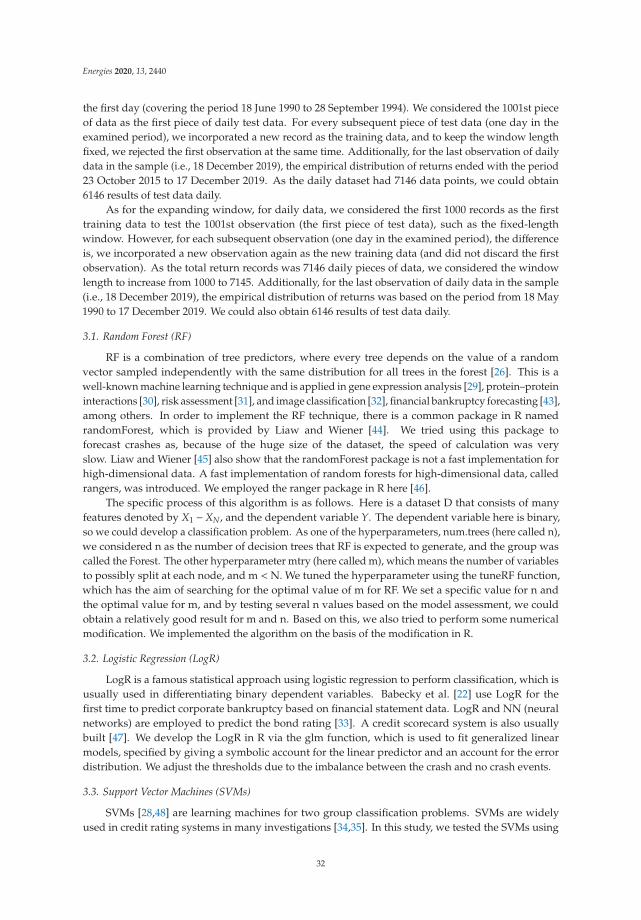
Energies 2020, 13, 2440

the first day (covering the period 18 June 1990 to 28 September 1994). We considered the 1001st pieceof data as the first piece of daily test data. For every subsequent piece of test data (one day in theexamined period), we incorporated a new record as the training data, and to keep the window lengthfixed, we rejected the first observation at the same time. Additionally, for the last observation of dailydata in the sample (i.e., 18 December 2019), the empirical distribution of returns ended with the period23 October 2015 to 17 December 2019. As the daily dataset had 7146 data points, we could obtain6146 results of test data daily.

As for the expanding window, for daily data, we considered the first 1000 records as the firsttraining data to test the 1001st observation (the first piece of test data), such as the fixed-lengthwindow. However, for each subsequent observation (one day in the examined period), the differenceis, we incorporated a new observation again as the new training data (and did not discard the firstobservation). As the total return records was 7146 daily pieces of data, we considered the windowlength to increase from 1000 to 7145. Additionally, for the last observation of daily data in the sample(i.e., 18 December 2019), the empirical distribution of returns was based on the period from 18 May1990 to 17 December 2019. We could also obtain 6146 results of test data daily.

3.1. Random Forest (RF)

RF is a combination of tree predictors, where every tree depends on the value of a randomvector sampled independently with the same distribution for all trees in the forest [26]. This is awell-known machine learning technique and is applied in gene expression analysis [29], protein–proteininteractions [30], risk assessment [31], and image classification [32], financial bankruptcy forecasting [43],among others. In order to implement the RF technique, there is a common package in R namedrandomForest, which is provided by Liaw and Wiener [44]. We tried using this package toforecast crashes as, because of the huge size of the dataset, the speed of calculation was veryslow. Liaw and Wiener [45] also show that the randomForest package is not a fast implementation forhigh-dimensional data. A fast implementation of random forests for high-dimensional data, calledrangers, was introduced. We employed the ranger package in R here [46].

The specific process of this algorithm is as follows. Here is a dataset D that consists of manyfeatures denoted by X1 −XN, and the dependent variable Y. The dependent variable here is binary,so we could develop a classification problem. As one of the hyperparameters, num.trees (here called n),we considered n as the number of decision trees that RF is expected to generate, and the group wascalled the Forest. The other hyperparameter mtry (here called m), which means the number of variablesto possibly split at each node, and m <N. We tuned the hyperparameter using the tuneRF function,which has the aim of searching for the optimal value of m for RF. We set a specific value for n andthe optimal value for m, and by testing several n values based on the model assessment, we couldobtain a relatively good result for m and n. Based on this, we also tried to perform some numericalmodification. We implemented the algorithm on the basis of the modification in R.

3.2. Logistic Regression (LogR)

LogR is a famous statistical approach using logistic regression to perform classification, which isusually used in differentiating binary dependent variables. Babecky et al. [22] use LogR for thefirst time to predict corporate bankruptcy based on financial statement data. LogR and NN (neuralnetworks) are employed to predict the bond rating [33]. A credit scorecard system is also usuallybuilt [47]. We develop the LogR in R via the glm function, which is used to fit generalized linearmodels, specified by giving a symbolic account for the linear predictor and an account for the errordistribution. We adjust the thresholds due to the imbalance between the crash and no crash events.

3.3. Support Vector Machines (SVMs)

SVMs [28,48] are learning machines for two group classification problems. SVMs are widelyused in credit rating systems in many investigations [34,35]. In this study, we tested the SVMs using

32

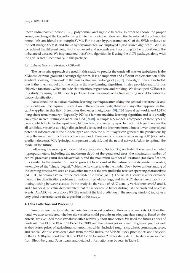
Energies 2020, 13, 2440

linear, radial basis function (RBF), polynomial, and sigmoid kernels. In order to choose the properkernel, we changed the kernel by using it into the moving window and, finally, selected the polynomialkernel. We considered soft-margin SVMs. For the cost hyperparameters, C, of the SVMs (relative tothe soft-margin SVMs), and the I3 hyperparameter, we employed a grid-search algorithm. We alsoconsidered the different weights of crash event and no crash event according to the proportion of theimbalanced dataset. We implemented this SVMs algorithm in R using the e1071 package, along withthe grid-search functionality, in this package.

3.4. Extreme Gradient Boosting (XGBoost)

The last main approach we used in this study to predict the crude oil market turbulence is theXGBoost (extreme gradient boosting) algorithm. It is an important and efficient implementation of thegradient boosting framework in the classification methodology of [36,37]. Two algorithms are included:one is the linear model and the other is the tree-learning algorithm. It also provides multifariousobjective functions, which include classification, regression, and ranking. We developed XGBoost inthis study by using the XGBoost R package. Here, we employed a tree-learning model to perform abinary classification.

We selected the statistical machine learning techniques after taking the general performance andthe calculation time required. In addition to the above methods, there are many other approaches thatcan be applied in this field. It includes the nearest neighbors [38], NN (neural network), and LSTM(long short-term memory). Especially, NN is a famous machine learning algorithm and it is broadlyemployed in credit rating classification filed [39,40]. A simple NN model is composed of three types oflayers, which includes the input layer, hidden layer, and output payer. In the input layer, there are theall candidate variables as a high dimensional vector, and the it is transformed into a lower-dimensionalpotential information in the hidden layer, and then the output layer can generate the predictions byusing the non-linear functions, such as a sigmoid. Even we could also consider using SGD (stochasticgradient descent), PCA (principal component analysis), and the neural network Adam to optimal themodel in the future.

Following the moving window that corresponds to Section 3.2, we tested the series of entailedhyperparameters, including the maximum depth of the generated trees, the maximum number ofcentral processing unit threads available, and the maximum number of iterations (for classification,it is similar to the number of trees to grow). On account of the nature of the dependent variable,we employed the “binary: logistic” objective function to train the model. For a better understanding ofthe learning process, we used an evaluation metric of the area under the receiver operating characteristic(AUROC) to obtain a value for the area under the curve (AUC). The AUROC curve is a performancemeasure for classification problems at various threshold settings, and the AUC shows the capability ofdistinguishing between classes. In the analysis, the value of AUC usually varies between 0.5 and 1,and a higher AUC value demonstrated that the model could better distinguish the crash and no crashevents. An AUC value of above 0.9 (the result of the last prediction in the moving window) indicates avery good performance of the algorithm in this study.

4. Data Collection and Processing

We considered various relative variables to forecast crashes in the crude oil markets. On the otherhand, we also considered whether the variables could provide an adequate data sample. Based on thecriteria, we excluded those variables with a relatively short time series. We used the futures prices ofcrude oil from 13 June 1986 to 18 December 2019, and the futures prices of natural gas and gold, as wellas the futures prices of agricultural commodities, which included rough rice, wheat, corn, sugar, cocoa,and canola. We also considered data from the VIX index, the S&P 500 stock price index, and the yieldof the USA 10-year bond from 8 June 1990 to 18 December 2019 for daily data. The data were sourcedfrom Bloomberg and Datastream, and detailed information can be seen in Table 1.

33

Energies 2020, 13, 2440

Table 1. Exploratory variables in the model.

Variable Data Data Source

Crude Oil WTI Crude Oil futures prices

Bloomberg

Natural Gas Henry Hub Natural Gas futures pricesVIX Index Chicago Board Options Exchange Volatility Index

Bond USA 10-year bond yieldStock S&P 500Gold Gold futures prices

Rough Rice Rough Rice futures prices

Wheat Wheat futures pricesDatastreamCorn Corn futures prices

Sugar Sugar futures pricesBloombergCocoa Cocoa futures prices

Canola Canola futures prices

Note: WTI is the West Texas intermediate. VIX is the Volatility Index.

As a result, we obtained a 30-year period for daily data, which included many crude oil futures pricecrashes. In this way, we filled the datasets with 7146 records for daily use. They provide the capabilityfor modeling contagion dynamics, financial markets, and commodity market interdependenciesover time.

In [3], the crisis event is detected based on an empirical distribution that is less than the 1%percentile. In order to obtain more crash event samples, we defined the crash event as less than the2.5% percentile of the empirical distribution due to the imbalanced dataset, following [15]. That is,we defined the “crash event” (CrashOILt ) at each working day. If the log return (hereafter return) of thecrude oil futures prices is less than the 2.5% percentile of the empirical distribution of the return, it canbe detected. We could obtain a binary variable of the crude oil futures price crashes as follows:

CrashOILt =

⎧⎪⎪⎨⎪⎪⎩ 1 if ROILt < E(ROILt

∣∣∣IOILt−1) −2√

Var(ROILt

∣∣∣IOILt−1)

0 otherwise, (1)

where ROILt is the log return of crude oil futures prices, IOILt−1 ={ROILt−1 , ROILt−2 · · ·

}is the information

set, E(ROILt

∣∣∣IOILt−1) denotes the sample mean of time t under condition IOILt−1 , and√

Var(ROILt

∣∣∣IOILt−1)

is the standard deviation of the crude oil futures prices of time t under condition IOILt−1 .Based on this, we employed two patterns of moving window to calculate the crash events. One is

the fixed-length window and the other is the expanding window.In terms of the fixed-length window, for daily data, we considered 1000 days (almost five years)

as the window length and calculated the initial empirical distribution of returns (starting from the firstday) based on the crude oil futures prices returns of the first 1000 observations (covering the periodfrom 16 June 1986 to 7 June 1990). We could detect if the 1001st is a crash event according the firstempirical distribution of daily returns. For each subsequent data point (day in the examined period),we recalculated the empirical distribution of returns and incorporated a new record, and in order tokeep the window length fixed, we rejected the first observation at the same time. The crash eventcan be identified when the return was below the 2.5% percentile of the new empirical distribution.In addition, for the last observation of daily data in the sample (i.e., 18 December 2019), the empiricaldistribution of returns ended with the period 23 October 2015 to 17 December 2019.

For the expanding window, for daily data, we could calculate the first empirical distributionbased on the first 1000 records to identify the 1001st observation, similar to the fixed-length window.However, for each subsequent observation (day in the examined period), the difference is that wecalculated the empirical distribution of returns and incorporated another new observation (we did notdiscard the first observation). As the total daily return records total 8152, we considered the window

34

Energies 2020, 13, 2440

length to increase from 1000 to 8151. In addition, for the last observation of daily data in the sample(i.e., 18 December 2019), the empirical distribution of returns was based on the period of 16 June 1986to 17 December 2019.

Ultimately, we obtained 7152 daily crash records (binary variables). We created the extendedvariables to take Lag1 to Lag5 of return (we elaborated these in Table 2), so we omitted the first sixcrash records.

Table 2. Extended variables. Returns are the log returns.

Variable Transformation

rash (binary variables) Lag1–Lag5, L5DIX Index Lag1–Lag5

Crude Oil futures prices

Lag1–Lag5, Lag1–Lag5 of returns

Natural Gas futures pricesUSA 10-year bond yield

S&P 500Gold futures prices

Rough Rice futures pricesWheat futures pricesCorn futures pricesSugar futures pricesCocoa futures pricesCanola futures prices

Note: L5D is the average of the crash events for the last five working days.

Figure 1 shows the number of crude oil market crashes for daily data during the selected 30-yearperiod. We could see several severe crashes in the daily and weekly frequencies, especially in 1990,1996, 2008, and 2015. The most severe crashes were in the global crisis of 2008, and the number ofcrashes was up to 35.

Figure 1. Number of crude oil market crashes for daily data (exceedance less than 2.5% percentile ofthe empirical distribution). Note: The fixed-length window means the length of the window was fixedat 1000 days, and the expanding window means the length of window increased from 1000 days to8151 days. The total daily data was 8152.

On the other hand, the raw data used are shown in Table 1. In order to get the most out of the rawdata and give full play to the machine learning models, we extended the raw variables and obtain theextended variables. To predict the crash events, we considered the previous data of crash events as afairly predictive indicator, so we also considered the binary variables of crash events.

We made the following transformations based on the exploratory variables to capture the subtlerdependencies and dynamics. Detailed information is displayed in Table 2.

35

Energies 2020, 13, 2440

1. We computed the lagged variables on a daily basis for each crash indicator, starting from one tofive days (Lag1–Lag 5).

2. Except for the Crash variable (binary variables) and VIX index (because it is a volatility index,we did not return to it), we took the return of the other variables. Then, using (i), we calculatedthe lagged variables of the return variables again.

3. We calculated the average number of crash events for the last five working days (L5D), accordingto the binary variables of crash events on a daily basis.

We also developed two predictive indicator datasets to see how much the performance of themachine learning models improves. One had only the Crash (Lag1–Lag5) and the crude oil futuresprices (Lag1–Lag 5, Lag1–Lag5 of returns) and the average of crash events for the last five working days(L5D; hereafter Dataset1), and the other had all predictive indicators (hereafter Dataset2). In Dataset1,there were 16 predictors, and in Dataset2, there were 121 predictors. For daily data, the dataset had7146 data points, spanning from 18 June 1990 to 18 December 2019.

5. Experimental Evaluation

After we obtained the confusion matrix of the various models for machine learning, we performedan experimental evaluation procedure. In other words, we showed the performance results for theevaluation of the models covering a long period (1994–2019 for daily data), which included severalcrash events.

5.1. Model Validation Measures

Classification accuracy is the main criterion for evaluating the efficiency of each approach and forselecting the most robust method according to discriminatory power. We provided several metrics thatare widely used to quantitatively assess the discriminatory power of each machine learning model.However, our dataset faced an issue of imbalanced amounts of the two classes, called imbalanced data.For example, in terms of the fixed length of the moving window for daily data, there were 6146 datapoints in total, in which only 205 were “CRASH.” Even if we obtained high classification accuracy,we could not consider the model to perform well. As such, there is a risk that the assessment norm weused may misinterpret based on the skewed class distribution. For the imbalanced data, we wanted toknow the capacity of predicting the minority of the dataset.

Bekkar et al. [49] presented a set of evaluation measures for model assessment over imbalanceddatasets. First, they obtained the sensitivity and specificity based on the confusion matrix andconsidered combined measures (G-means, likelihood ratios, F-measure balanced accuracy, discriminantpower, the Youden index, and the Matthews correlation coefficient). They also considered the graphicalperformance assessment (receiver operating characteristic (ROC) curve, area under curve, etc.). Due tothe application of the moving window, we could not obtain the AUC value based on the area underthe curve metrics, so we do not consider the AUC as the general metric. In a similar way, we donot use the graphical performance assessment. In machine learning, the two classes of forecastingmethod are assessed by the confusion matrix, such as in Table 3. The raw data represents the real valueof the class label, while the column represents the classifier prediction. In the imbalanced dataset,the observations of the minority class were defined as positive, and the observations of the majoritywere labeled negative. Here, positive means “CRASH,” negative means “NO CRASH.” Following [38],we adopted the sensitivity and specificity metrics, which are defined as follows.

Using the confusion matrix given by Table 3, we could calculate the sensitivity and specificityas follows:

Sensitivity =TP

TP + FN(2)

Speci f icity =TN

TN + FP(3)

36

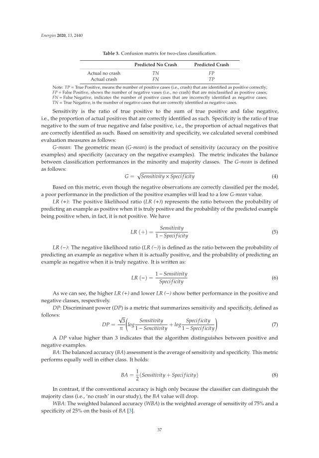
Energies 2020, 13, 2440

Table 3. Confusion matrix for two-class classification.

Predicted No Crash Predicted Crash

Actual no crash TN FPActual crash FN TP

Note: TP = True Positive, means the number of positive cases (i.e., crash) that are identified as positive correctly;FP = False Positive, shows the number of negative vases (i.e., no crash) that are misclassified as positive cases;FN = False Negative, indicates the number of positive cases that are incorrectly identified as negative cases;TN = True Negative, is the number of negative cases that are correctly identified as negative cases.

Sensitivity is the ratio of true positive to the sum of true positive and false negative,i.e., the proportion of actual positives that are correctly identified as such. Specificity is the ratio of truenegative to the sum of true negative and false positive, i.e., the proportion of actual negatives thatare correctly identified as such. Based on sensitivity and specificity, we calculated several combinedevaluation measures as follows:

G-mean: The geometric mean (G-mean) is the product of sensitivity (accuracy on the positiveexamples) and specificity (accuracy on the negative examples). The metric indicates the balancebetween classification performances in the minority and majority classes. The G-mean is definedas follows:

G =√

Sensitivity× Speci f icity (4)

Based on this metric, even though the negative observations are correctly classified per the model,a poor performance in the prediction of the positive examples will lead to a low G-mean value.

LR (+): The positive likelihood ratio (LR (+)) represents the ratio between the probability ofpredicting an example as positive when it is truly positive and the probability of the predicted examplebeing positive when, in fact, it is not positive. We have

LR (+) =Sensitivity

1− Speci f icity(5)

LR (−): The negative likelihood ratio (LR (−)) is defined as the ratio between the probability ofpredicting an example as negative when it is actually positive, and the probability of predicting anexample as negative when it is truly negative. It is written as:

LR (−) = 1− SensitivitySpeci f icity

(6)

As we can see, the higher LR (+) and lower LR (−) show better performance in the positive andnegative classes, respectively.

DP: Discriminant power (DP) is a metric that summarizes sensitivity and specificity, defined asfollows:

DP =

√3π

(log

Sensitivity1− Sencitivity

+ logSpeci f icity

1− Speci f icity

)(7)

A DP value higher than 3 indicates that the algorithm distinguishes between positive andnegative examples.

BA: The balanced accuracy (BA) assessment is the average of sensitivity and specificity. This metricperforms equally well in either class. It holds:

BA =12(Sensitivity + Speci f icity) (8)

In contrast, if the conventional accuracy is high only because the classifier can distinguish themajority class (i.e., ‘no crash’ in our study), the BA value will drop.

WBA: The weighted balanced accuracy (WBA) is the weighted average of sensitivity of 75% and aspecificity of 25% on the basis of BA [3].

37

Energies 2020, 13, 2440

Youden index: The Youden index γ measures the ability of the algorithm to avoid failure. It isdefined as:

γ = Sensitivity + Speci f icity− 1 (9)

Generally, a higher value of γ indicates a better ability to avoid misclassification.We used these criteria to perform a comprehensive measurement of the discriminative power of

each technique. On the basis of these outcomes, we inferred an optimal cutoff threshold of the predictedcrash probabilities for each fitted model, pertaining to the optimal sensitivity and specificity metrics.The results of each evaluation are displayed in Tables 4 and 5. As we could infer from Tables 4 and 5,both in Dataset1 and Dataset2, in terms of a fixed-length window, XGBoost could lead to the highestclassification accuracy, and in the case of an expanding window, LogR outperformed XGBoost.

Table 4. Model validation measures of daily data for Dataset1.

Window for Fixed-Length RF LogR SVMs XGBoost

G-mean 0.509 0.806 0.501 0.846LR (+) 7.852 5.028 3.750 8.339LR (−) 0.758 0.276 0.786 0.232

DP 0.560 0.695 0.374 0.858BA 0.617 0.807 0.599 0.848

WBA 0.443 0.786 0.435 0.819Youden 0.234 0.614 0.199 0.695

Window for Expanding RF LogR SVMs XGBoost

G-mean 0.345 0.590 0.406 0.463LR (+) 3.717 1.837 1.699 2.998LR (−) 0.907 0.716 0.915 0.832

DP 0.338 0.226 0.148 0.307BA 0.545 0.606 0.538 0.578

WBA 0.334 0.536 0.361 0.405Youden 0.090 0.212 0.076 0.155

Note: In Dataset1, there are 16 predictors. G-mean represents the geometric mean, LR (+) is the positive likelihoodratio, LR (−) denotes the negative likelihood ratio, DP denotes the discriminant power, BA represents the balancedaccuracy, and Youden denotes the Youden index I3.

Table 5. Model validation measures of daily data for Dataset2.

Window for Fixed-Length RF LogR SVMs XGBoost

G-mean 0.459 0.527 0.421 0.847LR (+) 3.766 3.690 10.116 5.124LR (−) 0.825 0.760 0.834 0.164

DP 0.364 0.378 0.597 0.824BA 0.582 0.610 0.581 0.847

WBA 0.403 0.456 0.381 0.855Youden 0.165 0.220 0.163 0.695

Window for Expanding RF LogR SVMs XGBoost

G-mean 0.402 0.560 0.296 0.366LR (+) 3.058 2.102 5.807 5.956LR (−) 0.878 0.754 0.925 0.883

DP 0.299 0.245 0.440 0.457BA 0.558 0.601 0.537 0.557

WBA 0.364 0.492 0.313 0.347Youden 0.115 0.201 0.074 0.114

Note: In Dataset2, there are 121 predictors. G-mean represents the geometric mean, LR (+) is the positive likelihoodratio, LR (−) denotes the negative likelihood ratio, DP denotes the discriminant power, BA represents the balancedaccuracy, and Youden denotes the Youden index I3.

38

Energies 2020, 13, 2440

5.2. Accuracy of the Generated Alarms

In conclusion, we provided a new insight into developing an early warning system for increasingawareness of an impending crash event in the crude oil futures prices market, using machine learningtechniques, which included random forest, logistic regression, support vector machine, and extremegradient boosting algorithms. We calculated an optimal oil futures price crash probability cut-offthreshold for each model, and when the predictive probabilities exceed the settled threshold, an alarmwill be generated.

As we can see from Tables 6 and 7, we obtained the final confusion matrix for all the evaluatedmodels. The results of the false alarm rate and detection rate are also shown. Concentrating on thebest-performing model, namely the XGBoost of the fixed-length window, by accepting a 9% false alarmrate, we succeeded in forecasting 79% of futures price crashes in the crude oil market for Dataset1.Under a false alarm rate of 17%, we could even predict 86% of crashes for Dataset2.

Table 6. Classification accuracy table for Dataset1.

Fixed-Length Window

RF pred LogR pred SVMs pred XGBoost pred

ture 0 1 Ture 0 1 ture 0 1 ture 0 1

0 5738 203 0 5036 905 0 5832 454 0 5378 563

1 150 55 1 48 157 1 175 65 1 43 162

Signal FAR DR Signal FAR DR Signal FAR DR Signal FAR DR

Rate 3% 27% Rate 15% 77% Rate 7% 27% Rate 9% 79%

Expanding Window

RF pred LogR pred SVMs pred XGBoost pred

ture 0 1 Ture 0 1 ture 0 1 ture 0 1

0 5801 199 0 4479 1521 0 5437 653 0 5534 466

1 128 18 1 78 68 1 119 27 1 112 34



Note: In Dataset1, there are 16 predictors. FAR represents false alarm rate, FAR = FPFP+TN ; DR represents detection

rate, and DR = TPTP+FN .

Table 7. Classification accuracy table for Dataset2.

Fixed-Length Window

RF pred LogR pred SVMs pred XGBoost Pred

ture 0 1 ture 0 1 ture 0 1 ture 0 1

0 5587 354 0 5454 487 0 5835 106 0 4940 1001

1 159 46 1 143 62 1 168 37 1 28 177



Expanding Window

RF pred LogR pred SVMs pred XGBoost Pred

ture 0 1 ture 0 1 ture 0 1 ture 0 1

0 5664 336 0 4905 1095 0 5908 92 0 5862 138

1 121 25 1 90 56 1 133 13 1 126 20



Note: In Dataset2, there were 121 predictors. FAR represents false alarm rate, FAR = FPFP+TN ; DR represents detection

rate, and DR = TPTP+FN .

39

Energies 2020, 13, 2440

6. Some Concluding Remarks

Financial crisis prediction plays a pivotal role for both practitioners and policymakers, as they caninfer crashes and recessions through an early warning system, being able to perform relevant actionsthat curtail the contagion crisis or preempt an economic crisis or recession.

Firstly, we chose the most significant financial market indicators to help forecasting and performchanges that capture the subtler dependencies and dynamics, and defined the crash event as less thanthe 2.5% percentile of the empirical distribution. Then we selected the statistical machine learningtechniques after taking the general performance and the calculation time required, and we developedthe evaluated models by tuning the hyperparameter and obtained the optimal performance of eachalgorithm. We employed the evaluation metrics that are broadly used to assess the discriminatorypower of a binary classifier on imbalanced datasets, finally.

Lean et al. [20] developed a general regression neural network (GRNN) currency forecasting model,and compared its performance with those of other forecasting methods. An early warning systemwas also developed using artificial neural networks (ANN), decision trees, and logistic regressionmodels to predict whether a crisis happens within the upcoming 12-month period [24]. Additionally,the result shows ANN has given superior results. Chatzis et al. [3] use a series of techniques includingclassification trees, SVMs, RF, NN, XGBoost, and deep neural networks to forecast the stock marketcrisis events, and find that deep neural networks built using the MXNET library is the best forecastingapproach. Our investigation concerns developing machine learning models that can be continuouslyretrained in moving window setup, which Chatzis et al. [3] do not challenge. Next, many previousinvestigations only use accuracy to measure the predictive ability of machine learning methods [20,24].However, in terms of the imbalanced dataset, we were concerned about whether the crisis or crashevent can be predicted precisely, rather than the no crisis or no crash event. Additionally, we regardedthe detection rate as important.

The main novel contribution of this empirical investigation to the existing literature is that it fillsthe gap of futures prices forecasting in the crude oil market, and we pioneered the use of a movingwindow in this field. We also made a comparison where the previous data were discarded.

Our empirical results show the following:

1. Except for the LogR for Dataset2, in other machine learning algorithms, the fixed-length windowshows a better performance than the expanding window. This indicates that discarding historicaldata is a better choice in forecasting the future.

2. XGBoost outperformed the rest of the employed approaches. It could even reach an 86% detectionrate using the fixed-length moving window for Dataset2.

3. The performances of Dataset1 and Dataset2 did not differ significantly, meaning the indicatorsthat are only about crude oil futures prices and crashes were very important.

These findings made our study much more attractive to researchers and practitioners working inpetroleum-related agencies. The result of XGBoost also provided strong evidence that it could offer agood starting point for developing an early warning system.

For future work, first, we will consider feature engineering and perform feature selection toimprove the accuracy of Dataset2. Chatzis et al. [3] show that deep neural networks significantlyincrease classification accuracy for forecasting stock market crisis events. Owing to the use of themoving window, we encountered some difficulties in coding when we wanted to implement the neuralnetwork technique. We will work hard to overcome this in future work.

Author Contributions: Investigation, Y.Z.; writing—original draft preparation, Y.Z.; writing—review and editing,S.H.; project administration, S.H.; funding acquisition, S.H. All authors have read and agreed to the publishedversion of the manuscript.


Acknowledgments: We are grateful to three anonymous referees for their helpful comments and suggestions.

40

Energies 2020, 13, 2440


References

1. Monthly Energy Review; U.S. Energy Information Administration. Available online: https://www.eia.gov/totalenergy/data/monthly/index.php (accessed on 10 February 2020).

2. Saggu, A.; Anukoonwattaka, W. Commodity Price Crash: Risks to Exports and Economic Growth inAsia-Pacific LDCs and LLDCs. United Nations ESCAP Trade Insights 2015, 6, 2617542.

3. Chatzis, P.S.; Siakoulis, V.; Petropoulos, A.; Stavroulakis, E.; Vlachogiannakis, N. Forecasting stock marketcrisis events using deep and statistical machine learning techniques. Expert Syst. Appl. 2018, 112, 353–371.[CrossRef]

4. Bluedorn, J.C.; Decreddin, J.; Terrones, M.E. Do asset price drops foreshadow recessions? Int. J. Forecast.2016, 32, 518–526. [CrossRef]

5. Koch, N.; Fuss, S.; Grosjean, G.; Edenhofer, O. Causes of the EU ETS price drop: Recession, CDM, renewablepolicies or a bit of everything?–New evidence. Energy Policy 2014, 73, 676–685. [CrossRef]

6. Alquist, R.; Kilian, L.; Vigfusson, R.J. Forecasting the price of oil. Handb. Econ. Forecast. 2013, 2, 427–507.7. Baumeister, C.; Kilian, L. Forecasting the real price of oil in a changing world: A forecast combination

approach. J. Bus. Econ. Stat. 2015, 33, 338–351. [CrossRef]8. Zhang, J.L.; Zhang, Y.J.; Zhang, L. A novel hybrid method for crude oil price forecasting. Energy Econ. 2015,

49, 649–659. [CrossRef]9. Xie, W.; Yu, L.; Xu, S.; Wang, S. A New Method for Crude Oil Price Forecasting Based on Support Vector

Machines. Comput. Sci. ICCS 2006, 3994, 444–451.10. Yu, L.; Wang, S.; Lai, K.K. Forecasting crude oil price with and EMD-based neural network ensemble learning

paradigm. Energy Econ. 2008, 30, 2623–2635. [CrossRef]11. Jammazi, R.; Aloui, C. Crude oil price forecasting: Experimental evidence from wavelet decomposition and

neural network modeling. Energy Econ. 2012, 34, 828–841. [CrossRef]12. Gabralla, L.A.; Jammazi, R.; Abraham, A. Oil price prediction using ensemble machine learning.

In Proceedings of the 2013 International Conference on Computing, Electrical and Electronic Engineering(ICCEEE), Khartoum, Sudan, 26–28 August 2013; pp. 674–679.

13. Gumus, M.; Kiran, M.S. Crude oil price forecasting using XGBoost. In Proceedings of the 2017 InternationalConference on Computer Science and Engineering (UBMK), Antalya, Turkey, 5–7 October 2017; pp. 1100–1103.

14. Chen, Y.; He, K.; Tso, G.K. Forecasting crude oil prices: A deep learning based model. Procedia Comput. Sci.2017, 122, 300–307. [CrossRef]

15. Bussiere, M.; Fratzscher, M. Towards a new early warning system of financial crises. J. Int. Money Financ.2006, 25, 953–973. [CrossRef]

16. Ye, M.; Zyren, J.; Shore, J. Forecasting short-run crude oil price using high- and low-inventory variables.Energy Policy 2006, 34, 2736–2743. [CrossRef]

17. Moshiri, S.; Foroutan, F. Forecasting nonlinear crude oil futures prices. Energy J. 2006, 27, 81–95. [CrossRef]18. Guo, X.; Li, D.; Zhang, A. Improved support vector machine oil price forecast model based on genetic

algorithm optimization parameters. AASRI Procedia 2012, 1, 525–530. [CrossRef]19. Niemira, M.P.; Saaty, T.L. An Analytic Network Process model for financial crisis forecasting. Int. J. Forecast

2004, 20, 573–587. [CrossRef]20. Yu, L.; Lai, K.K.; Wang, S.Y. Currency crisis forecasting with general regression neural networks. Int. J. Inf.

Technol. Decis Mak. 2006, 5, 437–454. [CrossRef]21. Davis, E.P.; Karim, D. Comparing early warning systems for banking crises. J. Financ. Stabil. 2008, 4, 89–120.

[CrossRef]22. Babecky, J.; Havranek, T.; Mateju, J.; Rusnak, M.; Smidkova, K.; Vasicek, B. Banking, debt and currency

crises: Early warning indicators for developed countries. ECB Work. Pap. 2012, 2162901. Available online:https://ssrn.com/abstract=2162901 (accessed on 10 February 2020). [CrossRef]

23. Dabrowski, J.J.; Beyers, C.; de Villiers, J.P. Systemic banking crisis early warning systems using dynamicBayesian networks. Expert Syst. Appl. 2016, 62, 225–242. [CrossRef]

24. Sevim, C.; Oztekin, A.; Bali, O.; Gumus, S.; Guresen, E. Developing an early warning system to predictcurrency crises. Eur. J. Oper. Res. 2014, 237, 1095–1104. [CrossRef]

41

Energies 2020, 13, 2440

25. Geng, R.; Bose, I.; Chen, X. Prediction of financial distress: An empirical study of listed Chinese companiesusing data mining. Eur. J. Oper. Res. 2015, 241, 236–247. [CrossRef]

26. Breiman, L. Random forests. Mach. Learn 2001, 45, 5–32. [CrossRef]27. Ohlson, J. Financial ratios and the probabilistic prediction of bankruptcy. J. Account. Res. 1980, 18, 109–131.

[CrossRef]28. Vapnik, V. Statistical Learning Theory; Springer: Berlin/Heidelberg, Germany, 1998.29. Diaz-Uriarte, R.; de Andres, S.A. Gene selection and classification of microarray data using random forest.

BMC Bioinform. 2006, 7, 3. [CrossRef]30. Chen, X.W.; Liu, M. Prediction of protein-protein interactions using random decision forest framework.

Bioinformatics 2005, 21, 4394–4400. [CrossRef]31. Malekipirbazari, M.; Aksakalli, V. Risk assessment in social lending via random forests. Expert Syst. Appl.

2015, 42, 4621–4631. [CrossRef]32. Bosch, A.; Zisserman, A.; Munoz, X. Image Classification using random forests and ferns. In Proceedings of

the IEEE 11th International Conference on Computer Vision, Rio de Janeiro, Brazil, 14–21 October 2007.33. Maher, J.J.; Sen, T.K. Predicting bond ratings using neural networks: A comparison with logistic regression.

Intell. Syst. Account. Financ. Manag. 1998, 6, 59–72. [CrossRef]34. Lee, Y.C. Application of support vector machines to corporate credit rating prediction. Expert Syst. Appl.

2007, 33, 67–74. [CrossRef]35. Kim, K.J.; Ahn, H. A corporate credit rating model using multi-class support vector machines with an ordinal

pairwise partitioning approach. Comput. Oper. Res. 2012, 39, 1800–1811. [CrossRef]36. Friedman, H.J.; Hastie, T.; Tibshirani, R. Additive logistic regression: A statistical view of boosting (With

discussion and a rejoinder by the authors). Ann. Stat. 2000, 28, 337–407. [CrossRef]37. Friedman, H.J. Greedy function approximation: A gradient boosting machine. Ann. Stat. 2001, 29, 1189–1232.

[CrossRef]38. Altman, N.S. An Introduction to kernel and Nearest–Neighbor Nonparametric Regression. Am. Stat. 1992,

46, 175–185.39. Huang, Z.; Chen, H.; Hsu, C.-J.; Chen, W.-H.; Wu, S. Credit rating analysis with support vector machines

and neural networks: A market comparative study. Decis. Support Syst. 2004, 37, 543–558. [CrossRef]40. Bennell, J.A.; Crabbe, D.; Thomas, S.; Gwilym, O. Modelling sovereign credit ratings: Neural networks

versus ordered probit. Expert Syst. Appl. 2006, 30, 415–425. [CrossRef]41. Kim, Y.H.; Chang, H.W. Forecasting the volatility of stock price index: A hybrid model integrating LSTM

with multiple GARCH-type models. Expert Syst. Appl. 2018, 103, 25–37. [CrossRef]42. Zhong, X.; Enke, D. Forecasting daily stock market return udsing dimensionality reduction. Expert Syst.

Appl. 2007, 67, 126–139. [CrossRef]43. Tanaka, K.; Higashide, T.; Kinkyo, T.; Hamori, S. Analyzing industry-level vulnerability by predicting

financial bankruptcy. Econ Inq. 2019, 57, 2017–2034. [CrossRef]44. Liaw, A.; Wiener, M. Classification and regression by random forest. R News 2002, 2, 18–22.45. Schwarz, D.F.; Konig, I.R.; Ziegler, A. On safari to random jungle: A fast implementation of random forests

for high-dimensional data. Bioinformatics 2010, 26, 1752–1758. [CrossRef] [PubMed]46. Wright, M.M.; Ziegler, A. ranger: A fast implementation of random forests for high dimensional data in C++

and R. J. Stat. Softw. 2015, 77, 1–17. [CrossRef]47. Dong, G.; Lai, K.K.; Yen, J. Credit scorecard on logistic regression with random coefficients. Procedia Comput.

Sci. 2010, 1, 2463–2468. [CrossRef]48. Cortes, C.; Vapnik, V. Support-vector networks. Mach. Learn 1995, 20, 273–297. [CrossRef]49. Bekkar, M.; Kheliouane, H.; Taklit, A. Evaluation measures for models assessment over imbalanced data sets.

J. Inform. Eng. App. 2013, 3, 10.


42

energies

Article

Do Machine Learning Techniques and DynamicMethods Help Forecast US Natural Gas Crises?

Wenting Zhang and Shigeyuki Hamori *

Graduate School of Economics, Kobe University, 2-1 Rokkodai, Nada-Ku, Kobe 657-8501, Japan;[email protected]* Correspondence: [email protected]


Abstract: Our study combines machine learning techniques and dynamic moving window andexpanding window methods to predict crises in the US natural gas market. Specifically, as machinelearning models, we employ extreme gradient boosting (XGboost), support vector machines (SVMs),a logistic regression (LogR), random forests (RFs), and neural networks (NNs). The data set used todevelop the model covers the period 1994 to 2019 and contains 121 explanatory variables, includingthose related to crude oil, stock markets, US bond and gold futures, the CBOE Volatility Index (VIX)index, and agriculture futures. To the best of our knowledge, this study is the first to combine machinelearning techniques with dynamic approaches to predict US natural gas crises. To improve the model’sprediction accuracy, we applied a suite of parameter-tuning methods (e.g., grid-search) to select thebest-performing hyperparameters for each model. Our empirical results demonstrated very goodprediction accuracy for US natural gas crises when combining the XGboost model with the dynamicmoving window method. We believe our findings will be useful to investors wanting to diversifytheir portfolios, as well as to policymakers wanting to take preemptive action to reduce losses.

Keywords: dynamic approaches; forecasting; logistic regression; random forests; support vectormachines; US natural gas crises; XGboost; neural networks

1. Introduction

To date, four international energy crises have occurred: The oil crisis of 1973, caused by theMiddle East War; the Iranian oil crisis of 1979, caused by the Islamic Revolution; the 1990 oil crisis,caused by the Gulf War; and the energy crisis in 2008 caused by the financial crisis. In addition to beinga subsystem of the national economy, the energy system incorporates the petroleum, coal, natural gas,and power economy. Birol [1] showed that the 2008 global financial crisis caused the energy demandin most countries to decrease, ultimately leading to the energy crisis. On the other hand, imbalancesbetween energy supply and demand are still the root cause of rising energy prices, and high energyprices were an underlying cause of the financial crisis.

Compared with fossil fuel oil and coal, natural gas is a more environment friendly and greenclean energy. As a result, natural gas has gained an increasingly prominent role in the global energymarket. As we know, people always use the settlement prices at the Henry Hub as benchmarks for theentire North American natural gas market and parts of the global liquid natural gas (LNG) market.According to the International Energy Agency (IEA), natural gas had a remarkable year in 2018,with a 4.6% increase in consumption, accounting for nearly half of the increase in global energy demand(https://www.iea.org/fuels-and-technologies/gas). Accurate predictions of crises in the natural gasmarket make it possible for investors and policymakers to minimize losses. Figure 1 shows some ofthe major events that affected US natural gas prices between 1994 and 2019.


Energies 2020, 13, 2371

Figure 1. The major crisis events related to US natural gas.

An early warning system (EWS) is a chain of information communication systems comprisingsensors, event detection, and decision subsystems. By employing such systems to detect crises beforethey occur, we can reduce false alarms [2]. An EWS must be able to send a clear signal about whetheran economic crisis is impending to complement the expert judgment of decision-makers. Edison [3]developed an operational EWS that successfully detects financial crises based on a signal approach [4,5].Ideally, an EWS should not ignore any crisis events but should minimize false alarms. However, the costof not sending a global crisis signal is much higher than the cost of an incorrect alert.

Machine learning refers to a scientific model in which computer systems rely on patternsand inference to perform specific tasks without applying explicit instructions. Machine learning isbecoming increasingly useful in finance. As banks and other financial institutions work to strengthensecurity, streamline processes, and forecast crises, machine learning is becoming their technologyof choice. Lin et al. [6] conducted a survey on machine learning in financial crisis prediction,using a machine learning algorithm to investigate the achievements and limitations of cy-predictionand credit-scoring models.

In this study, we propose a dynamic moving window and expanding window methodologythat incorporates extreme gradient boosting (XGboost), a support vector machine (SVM), a logisticregression (LogR), a random forest (RF), and a neural networks (NNs) as machine learning methods topredict US natural gas crises. To the best of our knowledge, this study is the first to combine dynamicmethodologies with machine learning to predict such crises. The main contributions of this studyare as follows:

• We employ dynamic methodologies to define a crisis, thus preventing extreme crisis events.• We use advanced machine learning techniques, including XGboost, neural networks, and other

traditional machine learning methods.• We combine dynamic methods with machine learning techniques to increase the prediction

accuracy of the model.• We employ novel model evaluation methodologies, and use daily data for the period 1994 to 2019.

The long period ensures enough data for the machine learning model, and allows us to checkwhether US natural gas crises are persistent and clustered.

Our main conclusion is that the combination of XGboost and the dynamic moving windowapproach performs well in predicting US natural gas crises, particularly in the partial variable case with

44

Energies 2020, 13, 2371

a moving window. In addition, LogR in the moving window method and NN in the expanding windowmethod do not perform badly in a partial variables situation whereas SVM in the moving window andLogR in the expanding window performance do not perform badly in the all variables situation.

The remainder of the paper proceeds as follows. Section 2 reviews relevant empirical works.In Section 3, we present the data and develop the model. In Section 4, we provide a brief description andtechnical analysis of the machine learning models employed in this study. In Section 5, we introducenovel model evaluation approaches. Here, we also present the empirical results for each machinelearning model. Section 6 concludes the paper. The Appendix A provides the XGboost variableimportance plots, the parameter tuning for the postulated SVM plots, the estimated LogR modelresults, and the RF variable importance plots.


Recent financial crises have highlighted their devastating effects on the economy, society,and politics. Therefore, being able to predict crises and disasters, particularly in areas, such asbanking, finance, business, medical, and others, means we can implement appropriate measures inadvance, and thus minimize losses. Chen et al. [7] considered value-at-risk (VaR) forecasting usinga computational Bayesian framework for a portfolio of four Asia-Pacific stock markets, showing thatthe Autoregressive Conditional Heteroscedasticity (GARCH) model outperforms stochastic volatilitymodels before and after the crises. Bagheri et al. [8] proposed a new hybrid intelligence approachto predict financial periods for the foreign exchange market, finding that it performs well for priceforecasting. Niemira and Saaty [9] developed an imbalanced crisis turning point model based on theanalytical network process framework to forecast the probability of crises, finding this method to bemore flexible and comprehensive than traditional methods. Chiang et al. [10] showed that traderscould generate higher returns by employing their proposed adaptive decision support system model.

An energy crisis refers to an energy shortage caused by rising energy prices, and energy andfinancial crises have mutual effects. Gorucu [11] employed an artificial neural network (ANN) to evaluateand predict natural gas consumption in Ankara, Turkey, examining the factors affecting the output, andthen training the ANN to determine the optimal parameters to predict gas consumption, achieving agood performance. Xie et al. [12] used an SVM to forecast crude oil prices, finding that it outperformsboth auto regressive integrated moving average and back-propagation neural network models.

Regarding crisis prediction, there are currently three international financial crisis early warningmodels. First, the discrete choice (probit or logit) model, developed by Frankel and Rose [13], has beenused to model financial contagion by Bae et al. [14]. Second, Sachs et al. [15] developed an STVcross-section regression model, finding that the depreciation of the real exchange rate, growth ofdomestic private loans, and international reserves/M2 (a calculation of the money supply that includescash and checking deposits as well as near money) are important indicators of whether a country willexperience a financial crisis. Third, Kaminsky and Reinhart [5] developed a signaling approach-KLRmodel that monitors the evolution of several indicators that approach to show unusual behavior inperiods preceding a crisis. Furthermore, Knedlik and Schweinitz [16] investigated debt crises in Europeby applying a signal approach, finding that a broad composite indicator has the highest predictivepower. Numerous works have since extended these three models, thus improving the early warningsystem. Based on the multinomial logit model, Bussiere and Fratzscher [17] developed a new earlywarning system (EWS) model for financial crises. Their results show that employing the proposedEWS substantially improves the ability to forecast financial crises, and that their model would havepredicted crises correctly in emerging markets between 1993 and 2001. Xu et al. [18] combined an RFand a wavelet transform in a new EWS to forecast currency crises, finding that real exchange rateappreciation and overvaluation can be measured over a period of 16 to 32 months. Saleh et al. [19]applied a new EWS model for systemic financial fragility and near crises in The Organisation forEconomic Co-operation and Development (OECD) countries over a 27-year period, finding that themodel has significant implications for financial stability and regulation.

45

Energies 2020, 13, 2371

Researchers are increasingly combining EWSs with machine learning techniques to predictfinancial crises. Ahn et al. [20] extended the EWS classification method to a traditional-type crisis,using an SVM to forecast financial crises. As such, they proved that an SVM is an efficient classifier.Sevim et al. [21] developed three EWSs, based on an ANN, a decision tree, and a LogR model,respectively, to predict currency crises, finding that the decision tree model can predict crises up toa year ahead with approximately 95% accuracy. In order to predict currency crises, Lin et al. [22]developed a hybrid causal model, which is integrated by the learning ability of a neural networkwith the inference mechanism of a fuzzy logit model, showing that this approach is promising interms of preventing currency crises. Finally, Chatzis et al. [23] employed a classification tree, SVM, RF,neural network, XGboost, and deep neural network to forecast stock market crises. They show thatdeep neural networks increase the classification accuracy significantly, and propose an efficient globalsystemic early warning tool.

Few studies have used machine learning methods with moving windows to predict financialcrises. However, studies have focused on other classification methods. Bolbol et al. [24] combineda moving window method with an SVM to classify Global Positioning System (GPS) data into differenttransportation modes. Chou and Ngo [25] combined the time-series sliding window with the machinelearning system to predict real-time building energy-consumption data, showing that the model canpotentially predict building energy consumption using big data.

From the aforementioned literature, we can see that the methodologies proposed here offer clearinnovations and advantages. Thus, we compared the predictive ability of the following models: XGboost,a SVM, a LogR, a RF, and a NN. In addition, we used a moving window and an expanding windowapproach. Furthermore, we investigated the effects of explanatory variables on the models’ predictiveability by splitting the variables into two categories—natural gas-related predictors (16 predictors), and allpredictors (121 predictors)—to compare their prediction accuracy separately. To the best of our knowledge,our study is the first to analyze US natural gas market crises by combining machine learning techniqueswith dynamic forecasting methods (the moving window and expanding window method).

3. Data

3.1. Data Collection

We employed daily data to model US natural gas market crises, focusing on the US crude oil,stock, commodity, and agriculture markets, where the transmission of extreme events is stronger.In order to obtain an adequate daily data sample for machine learning, we collected data from manydifferent sources and databases (see Table 1).

Table 1. Variables in the model.

Variables Raw Data Data Source

Natural Gas Henry Hub Natural Gas Futures (USD/Million Btu) BloombergCrude oil Crude Oil WTI Futures (USD/Barrel) Bloomberg

Stock S&P 500 Index BloombergBond United States 10-Year Bond Yield BloombergGold Gold Futures Price BloombergVix CBOE Volatility Index Bloomberg

Canola Canola Futures Price BloombergCocoa US Cocoa Futures Price BloombergSugar No.11 Sugar Futures Price BloombergRice Rough Rice Futures Price BloombergCorn Corn Futures Price DataStream

Wheat US Wheat Futures Price DataStream

The raw data included the most sensitive market variables from the energy, stock, commodity,and agriculture markets. To remove the effect of the exchange rate on our results, we consolidated the

46

Energies 2020, 13, 2371

currency units of the variables into a dollar currency unit. Then, because natural gas has the shortestperiod of daily data (8 June 1990–18 December 2019), we focused on this period for all variables. Finally,we obtained a raw daily price data set with 7152 records. This data set enabled us to model contagiondynamics and financial market interdependence across natural gas-related variables and over time.In order to facilitate the reading of this paper, we named the professional items as exhibited in Table 2.

Table 2. Nomenclature for professional items.

Nomenclature

pt Natural Gas Daily Pricert Natural Gas Daily Returnμt 1000-Day Moving and Expanding Window Average return at time tσt 1000-Day Moving and Expanding Window Standard deviation at time tNCt US Natural gas crises at time tXGboost Extreme Gradient BoostingSVM Support Vector MachinesLogR Logistic RegressionRF Random ForestsNN Neural NetworksG-mean The geometric meanLP The positive likelihood ratioLN The negative likelihood ratioDP The discriminant powerBA Balanced accuracyWBA The weighted balance accuracyDM-test Diebold-Mariano Test

3.2. Data Processing

In Section 3.1, we described the raw data and the prices of the variables. Our goal was to predictnext-day crisis events in the US natural gas market using machine learning. Therefore, we needed todefine a “crisis event” for natural gas. We also wanted to apply the moving window and expandingwindow methods in our model. We illustrate these two methods below (see Table 3) [26].

Table 3. Daily data set for the moving window and expanding window.

Variable Names Numerical Formula

Natural Gas Daily Price ptNatural Gas Daily Return rt = ln(pt) − ln(pt−1)

1000-Day Moving Window Average μt+1000 =∑t+999

t rt1000 (t = 1, 2, . . . , 6151)

1000-Day Expanding Window Average μi+1001 =∑i+1000

1 rt

i+1000 (i = 0, 1, . . . 6150, t = 1, 2 . . . . 6151)

1000-Day Moving Window Standard Deviation σt+1000 =

√var(

t+999∑t

rt) (t = 1, 2, . . . , 6151)

1000-Day Expanding Window Standard Deviation σi+1001 =

√var(

i+1000∑1

rt) (i = 0, 1, . . . 6150, t = 1, 2 . . . . 6151)

We set a 1000-day window, covering five years of daily data. First, we employed the logarithmicdifference method to compute the daily return of natural gas. Then, in the daily data set, we calculatedthe initial empirical distribution of the return on 22 September 1994, based on the daily returns of the first1000 observations (covering the period 11 June 1990–21 September 1994, which is a 1000-day window).Next, for the moving window method, for each subsequent record, we fixed the number of days(1000 days in the daily data set), and moved the window forward by one day. Then, we recalculatedthe empirical distribution of the returns based on the new period. Thus, for the last observation inthe daily data (18 December 2019), the empirical distribution of the returns was based on the period23 November 2015 to 17 December 2019 (i.e., 1000 days). In contrast, for the expanding window

47

Energies 2020, 13, 2371

method, for each subsequent record, we increased the size of the window by one day. Then, we againrecalculated the empirical distribution of the returns, including the new observation. Hence, for thelast observation in the daily data (18 December 2019), the empirical distribution of the returns wasbased on the period 11 June 1990, to 17 December 2019 (i.e., 7150 days).

Thus, we obtained the preliminary processed data from which to calculate the “crisis events.”Bussiere and Fratzscher [17] developed an EWS model based on a multinomial logit model to forecastfinancial crises, using EMPi,t to define a currency crisis for each country i and period t. Patel andSarkar [27], Coudert and Gex [28], and Li et al. [29] used CMAXt, defined as the ratio of an index levelat month t to the maximum index level for the period up to month t. Here, we employed the return ofnatural gas, defined as follows:

rt = ln(pt) − ln(pt−1), (1)

where pt is the price of natural gas on day t. Next, as in Bussiere and Fratzscher [17], we defined NCt asa crisis event when the natural gas return rt is less than two standard deviations below its mean value:

NCt =

{1, i f NCt ≤ μt − 2σt

0, otherwise, (2)

where μt and σt were calculated based on Table 3. The former is the mean value calculated by themoving window or expanding window on day t. Similarly, the latter denotes the standard deviationcalculated by the corresponding methods. We plotted the crises processing procedure, as shown inFigure 2. After processing these data, we obtained two predicted/dependent variables in the dailydata set. These constitute binary indicators that take the value of 1 when a crisis occurs in the USnatural gas market on the following day, and 0 otherwise. Based on these formulae, Table 4 andFigure 3 summarize the crisis events between 22 September 1994 and 18 December 2019.

Table 4. Crisis events in the US natural gas market.

Year Number of Crises

Moving Window Expanding Window1994 2 21995 6 61996 16 181997 6 81998 3 41999 2 32000 6 72001 13 142002 3 32003 8 82004 3 52005 1 12006 7 82007 2 22008 7 52009 9 92010 0 02011 1 02012 3 22013 1 02014 10 42015 6 22016 7 02017 4 22018 10 72019 4 3

Total 140 123

48

Energies 2020, 13, 2371

Figure 2. US natural gas crises processing.

Figure 3. Number of crises in the US natural gas market.

49

Energies 2020, 13, 2371

We have outlined the exploratory binary variables in the daily data set using the moving windowand expanding window methods. Next, we constructed the independent variables for our machinelearning model. In particular, to capture the subtle dynamics and correlations, we performed thefollowing transformation:

1. We calculated the average number of crises during the previous five working days, based on thetotal number of crisis events.

2. We used the logarithmic difference method to derive the continuously compounded daily returnfor the prices of natural gas, crude oil, bond yield, gold, canola, cocoa, sugar, rice, corn, and wheat.

3. We calculated the lagged variables for each crisis indicator, for one to five days. Specifically,we considered these lags (lag1 to lag5) for the crisis itself, the returns on all variables except theVIX index, and the returns on all variables including the VIX index.

After the above processing, we obtained two summary tables of daily data for the period28 February 1994 to 18 December 2019, yielding 6146 records and 121 predictors. The firsttable determines crises using the moving window method, and the second uses the expandingwindow method.

4. Model Development

As already discussed, we combined the moving window method, expanding window method,and machine learning to predict crisis events. In addition, we used a moving window and expandingwindow in the data processing step. Therefore, we employed corresponding methods to develop ourmodel using machine learning. By doing so, we derived dynamic results and improved the accuracyof the model prediction [25]. To maintain the initial number of windows, we employed 1000 days asthe initial number of days for the moving window (fixed) and the expanding window (increasing byone day). In order to combine machine learning with the two window methods, we inserted loopstatements into the machine learning model to perform 5146 iterations. For both methods, we set alldata in the window as the training data set, and set the day following the final day in the training dataset as the test data set. For example, in the final loop calculation, the training data set for the movingwindow method covers the period 19 November 2015 to 17 December 2019 (1000 days), and the testdata is that of 18 December 2019; for the expanding window method, the training data set covers theperiod 29 September 1994 to 17 December 2019 (6145 days), and the test data is that of 18 December2019. Therefore, we derived a confusion matrix for crisis prediction once the loops were complete.

Next, we chose our methods following Chatzis et al. [23], deciding on the following: XGboost [30],SVM [31], LogR [32], RF [33–35], and NN [36]. We split the explanatory variables into two types tocompare the predictions: A natural gas-related variable (the average number of crises during theprevious five working days, lags 1 to 5 of crises, and lags 1 to 5 of the prices and returns of naturalgas, yielding 16 predictors), and all variables (121 predictors, including natural gas-related variables).In the following section, we describe the development process and the parameter tuning for each model.

4.1. Extreme Gradient Boosting

XGboost is not only an improvement algorithm on the boosting algorithm based ongradient-boosted decision trees, and the internal decision tree uses a regression tree, but also an efficientand prolongable development of the gradient boosting framework [37]. It supports multiple kinds ofobjective functions, like regression, classification, ranking, and so on. Furthermore, in terms of modelaccuracy, efficiency, and scalability, XGboost outperforms RFs and NNs [23]. In our study, we employedthe XGboost R package developed by Chen and He [30].

In order to increase the accuracy of the model prediction, we employed a (five-fold) cross-validationmethod to debug a series of vital hyperparameters. In order to build the classification tree, we determinedthe maximum depth of the tree, minimum number of observations in a terminal node, and size ofthe subsampling for both window methods. We also tuned the hyperparameter γ, which controls the

50

Energies 2020, 13, 2371

minimum reduction in the loss function required to grow a new node in a tree, and reduces overfittingthe model. In addition, we tuned α (the L1 regulation term on the weights) and λ (the L2 regulationterm on weights). Because of the binary nature of our dependent variable, we applied the LogRobjective function for the binary classification to train the model. We also calculated the area under thecurve (AUC) of our model, which is equal to the probability that the classifier ranks randomly selectedpositive instances higher than randomly selected negative instances. In our model training, when weemployed the moving window method, the AUC values were above 0.8, regardless of whether weused 16 natural gas-related explanatory variables or 121 explanatory variables, indicating a very goodperformance. However, we derived an AUC of only 0.67 when applying the expanding windowmethod, indicating a poor performance for the combination of this and the XGboost method.

Because we used the moving window and expanding window methods in our study, we cannotshow every XGboost variable importance plot, because there were more than 5000 plots after theloop calculation. Therefore, we present the plots for the last step of the loop in the Appendix A.Here, Figures A1 and A2 show that lag5 of the natural gas price is the most important variable inthe moving window method. However, lag2 of the natural gas return is the most important in theexpanding window method.

4.2. Support Vector Machines

Erdogan [38] applied an SVM [31] to analyze the financial ratio in bankruptcy, finding that theSVM with a Gaussian kernel is capable of predicting bankruptcy crises. This is because the SVM hasa regularization parameter, which controls overfitting. Furthermore, using an appropriate kernelfunction, we can solve many complex problems. An SVM scales relatively well to high-dimensionaldata. Therefore, it is widely used in financial crisis prediction, handwriting recognition, and so on.

In our study, we used sigmoid, polynomial, radial basis function, and linear kernels to evaluatea soft-margin SVM, finding that the sigmoid function performs optimally. In order to select theoptimal hyperparameter (e.g., γ, the free parameter of the Gaussian radial basis function, and c,the cost hyperparameter of the SVM, which involves a trading error penalty for stability), we appliedcross-validation. We selected the optimal values of these hyperparameters using the grid-searchmethodology. We implemented the SVM model using the e1071 package in R, employing the tuningfunction in the e1071 package to tune the grid-search hyperparameter.

Unlike the XGboost methodology, we could tune the parameters γ and c of the daily data set beforeexecuting the loop calculation. The plots of the parameter tuning for the SVM model are providedin the Appendix A. Figures A3 and A4 show the hyperparameters γ (x-axis) and c (y-axis) using thegrid-search method in the SVM model. The parameter c is the cost of a misclassification. As shown,a large c yields a low bias and a high variance, because it penalizes the cost of a misclassification.In contrast, a small c yields a high bias and a low variance. The goal is to find a balance between“not too strict” and “not too loose”. For γ, the parameter of the Gaussian kernel, low values mean “far”and high values mean “close”. When γ is too small, the model will be constrained and will not be ableto determine the “shape” of the data. In contrast, an excessively large γwill lead to the radius of thearea of influence of the support vectors only including the support vector itself. In general, for an SVM,a high value of gamma leads to greater accuracy but biased results, and vice versa. Similarly, a largevalue of the cost parameter (c) indicates poor accuracy but low bias, and vice versa.

4.3. Logistic Regression

In statistics, the LogR algorithm is widely applied for modeling the probability of a certain classor event existing, such as crisis/no crisis, healthy/sick or win/lose, and so on. The LogR is a statisticalmodel, which applies a logistic function to model a binary dependent variable in its basic form.Ohlson [32] employed a LogR to predict corporate bankruptcy using publicly available financial data.Yap et al. [39] employed a LogR to predict corporate failures in Malaysia over a 10-year period, findingthe method to be very effective and reliable. In our study, we employed the glm function in R, following

51

Energies 2020, 13, 2371

Hothorn and Everitt [40]. In addition, because the output of a LogR is a probability, we selectedoptimistic thresholds for the two window methods separately when predicting crises. We also employeda stepwise selection method to identify the statistically significant variables. However, this did notresult in a good performance. Therefore, we did not consider the stepwise method further.

As before, we summarize some of the outcomes of our analysis in the Appendix A. Here, Tables A1and A2 exhibit some of the outcomes of our analysis and we also present the plot of the final step ofthe loop calculation, showing only the intentionality of some of the variables. As shown, whether inthe partial variables case or the all variables case, the lagged value and the average of five days ofcrisis are the most intentional.

4.4. Random Forests

An RF [33–35] is an advanced learning algorithm employed for both classification and regressioncreated by Ho [41]. A forest in the RF model is made up of trees, where a greater number of treesdenotes a more robust forest. The RF algorithm creates decision trees from data samples, obtainsa prediction from each, and selects the best solution by means of voting. Compared with a singledecision tree, this is an ensemble method. Because it can reduce overfitting by averaging the results.RFs are known as bagging or bootstrap aggregation methods. By identifying the best segmentationfeature from the random subset of available features, further randomness can be introduced.

In RF, a large number of predictors can provide strong generalization; our model contains121 predictors. In order to improve the accuracy of model prediction, we must obtain an optimalvalue of m, the number of variables available for splitting at each tree node. If m is relatively low,then both the inter-tree correlation and the strength of each tree will decrease. To find the optimalvalue, we employed the grid-search method. In addition to m, we tuned the number of trees using thegrid-search method. To reduce the computing time, we applied the ranger package in R to constructthe prediction model, employing the tuneRF function in the randomForest package.

We provide the RF variable importance plots in the last loop calculation in Appendix A.In Figures A5 and A6, we present the importance of each indicator for the classification outcome.The obtained ranking is based on the mean decrease in the Gini. This is the average value of the totalreduction of variables in node impurities, weighted by the proportion of samples that reach the node ineach decision tree in RF. Here, a higher mean decrease in the Gini indicates higher variable importance.We found that in the partial variables case, the lags of the natural gas price and the natural gas returnare relatively important; however, in the case of all variables, this was not the case.

4.5. Neural Networks

In the field of machine learning and cognitive science, an NN [34] is a mathematical orcomputational model, which imitates the structure and function of a biological neural network(animal central nervous system, especially the brain), employed to estimate or approximate functions.Like other machine learning methods, NN have been used to solve a variety of problems, such ascredit rating classification problems, speech recognition, and so on. The most usually consideredmultilayer feedforward network is composed of three types of layers. First, in the input layer, manyneurons accept a large number of nonlinear input messages. The input message is called the inputvector. Second, the hidden layer, which is the various layers composed of many neurons and linksbetween the input layer and output layer. The hidden layer can have one or more layers. The numberof neurons in the hidden layer is indefinite, but the greater the number, the more nonlinear the NNbecomes, so that the robustness of the neural network is more significant. Third, in the output layer,messages are transmitted, analyzed, and weighed in the neuron link to form the output. The outputmessage is called the output vector.

In order to increase the accuracy of the model prediction, we employed the grid-search method tofind the best parameter size and decay. The parameter size is the number of units in the hidden layer

52

Energies 2020, 13, 2371

and parameter decay is the regularization parameter to avoid over-fitting. We used nnet package in Rto develop the model prediction.

5. Model Evaluation

In this section, we evaluate the robustness of our methods by performing a comprehensiveexperimental evaluation procedure. Specifically, we use several criteria to evaluate the aforementionedmodels in terms of crisis event prediction.

5.1. Verification Methods

Accuracy is measured by the discriminating power of the rating power of the rating system.It is the most commonly used indicator for classification, and it estimates the overall effectivenessof an approach by estimating the probability of the true value of the class label. In the followingsection, we introduce a series of indicators that are widely employed to quantitatively estimate thediscriminatory power of each model.

In machine learning, we can derive a square 2 × 2 matrix, as shown in Table 5, which we used asthe basis of our research.

Table 5. Confusion matrix for two classes classification.

Predicted 0 Predicted 1

Actual 0 TN (number of True Negatives) FP (number of False Positives)Actual 1 FN (number of False Negatives) TP (number of True Positives)

Notes: 0 refers to “No crisis”; 1 refers to “Crisis”; Predicted 0 refers to a predicted value of 0, Predicted 1 refers toa predicted value of 1; Actual 0 refers to a true value of 0; Actual 1 refers to a true value of 1; TN = True Negative:the number of negative cases (i.e., no crisis) correctly identified as negative cases; FP = False Positive: the number ofnegative cases (i.e., no crisis) incorrectly identified as positive cases; FN = False Negative: the number of positivecases (i.e., crisis) misclassified as negative cases; TP = True Positive: the number of positive cases (i.e., crisis) correctlyidentified as positive.

Bekkar et al. [42] state that imbalanced data learning is one of the challenging problems in datamining, and consider that skewed classes in the level distribution can lead to misleading assessmentmethods and, thus, bias in the classification. To resolve this problem, they present a series of alternativesfor imbalanced data learning assessment, which we introduce below.

Bekkar et al. [42] defined sensitivity and specificity as follows:

Sensitivity (or Recall) =TP

TP + FN; Speci f icity =

TNTN + FP

. (3)

Sensitivity and specificity assess the effectiveness of an algorithm on a single class for positiveand negative outcomes, respectively. The evaluation measures are as follows:

• G-mean: The geometric mean is the product of the sensitivity and specificity. This metric canindicate the valance between the classification performance of the majority and minority classes.In addition, the G-mean measures the degree to which we avoid overfitting on the negative class,and the degree to which the positive class is marginalized. The formula is as follows:

G−mean =√

Sensitivity× Speci f icity. (4)

Here, a low G-mean value means the prediction performance of the positive cases is poor, even ifthe negative cases are correctly classified by the algorithm.

53

Energies 2020, 13, 2371

• LP: The positive likelihood ratio is that between the probability of predicting an example aspositive when it is really positive, and the probability of a positive prediction when it is notpositive. The formula is as follows:

LP =TP/(TP + FN)

FP/(FP + TN)=

Sensitivity1− Speci f icity

. (5)

• LN: The negative likelihood ratio is that between the probability of predicting an example asnegative when it is really positive, and the probability of predicting a case as negative when it isactually negative. The formula is as follows:

LN =FN/(TP + FN)

TN/(FP + TN)=

1− SensitivitySpeci f icity

. (6)

• DP: The discriminant power, a measure that summarizes sensitivity and specificity. The formulais as follows:

DP =

√3π

(log

Sensitivity1− Sensitivity

− logSpeci f icity

1− Speci f icity

). (7)

DP values can evaluate the degree to which the algorithm differentiates between positive andnegative cases. DP values lower than one indicate that the algorithm differentiates poorly between thetwo, and values higher than three indicate that it performs well.

• BA: Balanced accuracy, calculated as the average of the sensitivity and specificity. The algorithmis as follows:

BA =12(Sensitivity + Speci f icity). (8)

If the classifier performs equally well in both classes, this term reduces to the conventionalaccuracy measure. However, if the classification performs well in the majority class (in our study,“no crisis”), the balance accuracy will drop sharply. Therefore, the BA considers the majority class andminority class (in our study, “crisis”) equally.

• WBA: The weighted balance accuracy. Under the weighting scheme 75%: 25%, the WBAemphasizes sensitivity over specificity, and is defined by Chatzis et al. [23] as follows:

WBA = 0.75 ∗ Sensitivity + 0.25 ∗ Speci f icity. (9)

• Youden’ s γ: An index that evaluates the ability of an algorithm to avoid failure. This indexincorporates the connection between sensitivity and specificity, as well as a linear correspondencewith balanced accuracy:

γ = Sensitivity− (1− Speci f icity) = 2 ∗ BA− 1. (10)

• F-measure: The F-measure employs the same contingency matrix as that of relative usefulness.Powers [43] shows that an optimal prediction implies an F-measure of one. The formula isas follows:

F−measure =TP

TP +(FP+FN)

2

. (11)

• DM-test: The Diebold–Mariano test is a quantitative approach to evaluate the forecast accuracyof US natural gas crises predicting models in our paper [44]. In our paper, the DM-test can helpus to discriminate the significant differences of the predicting accuracy between the XGboost,

54

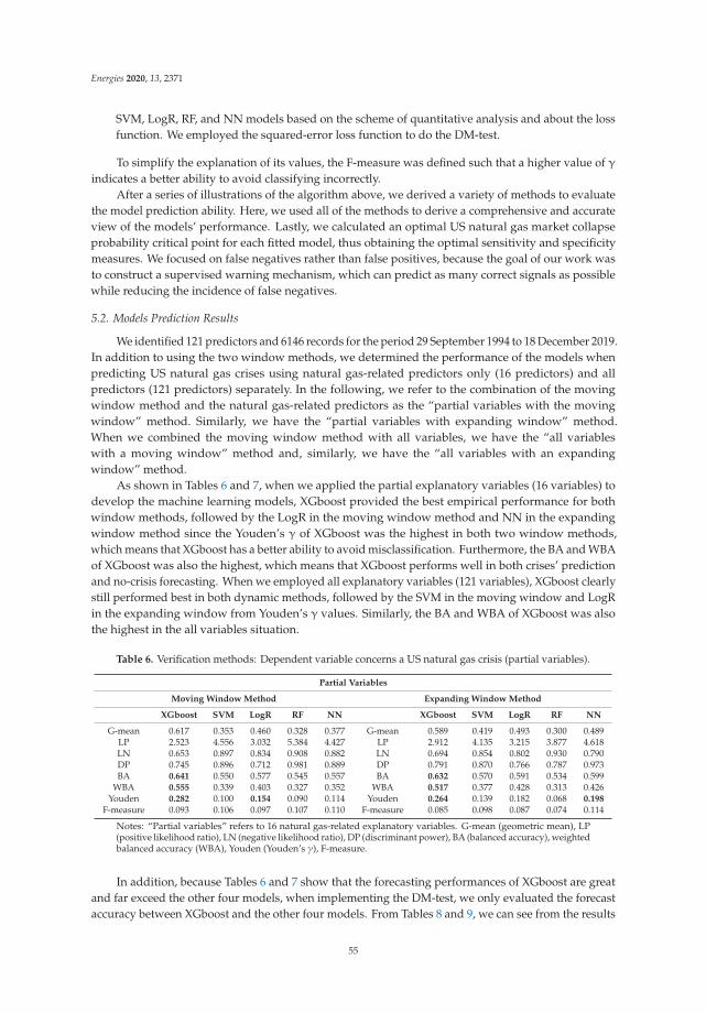
Energies 2020, 13, 2371

SVM, LogR, RF, and NN models based on the scheme of quantitative analysis and about the lossfunction. We employed the squared-error loss function to do the DM-test.

To simplify the explanation of its values, the F-measure was defined such that a higher value of γindicates a better ability to avoid classifying incorrectly.

After a series of illustrations of the algorithm above, we derived a variety of methods to evaluatethe model prediction ability. Here, we used all of the methods to derive a comprehensive and accurateview of the models’ performance. Lastly, we calculated an optimal US natural gas market collapseprobability critical point for each fitted model, thus obtaining the optimal sensitivity and specificitymeasures. We focused on false negatives rather than false positives, because the goal of our work wasto construct a supervised warning mechanism, which can predict as many correct signals as possiblewhile reducing the incidence of false negatives.

5.2. Models Prediction Results

We identified 121 predictors and 6146 records for the period 29 September 1994 to 18 December 2019.In addition to using the two window methods, we determined the performance of the models whenpredicting US natural gas crises using natural gas-related predictors only (16 predictors) and allpredictors (121 predictors) separately. In the following, we refer to the combination of the movingwindow method and the natural gas-related predictors as the “partial variables with the movingwindow” method. Similarly, we have the “partial variables with expanding window” method.When we combined the moving window method with all variables, we have the “all variableswith a moving window” method and, similarly, we have the “all variables with an expandingwindow” method.

As shown in Tables 6 and 7, when we applied the partial explanatory variables (16 variables) todevelop the machine learning models, XGboost provided the best empirical performance for bothwindow methods, followed by the LogR in the moving window method and NN in the expandingwindow method since the Youden’s γ of XGboost was the highest in both two window methods,which means that XGboost has a better ability to avoid misclassification. Furthermore, the BA and WBAof XGboost was also the highest, which means that XGboost performs well in both crises’ predictionand no-crisis forecasting. When we employed all explanatory variables (121 variables), XGboost clearlystill performed best in both dynamic methods, followed by the SVM in the moving window and LogRin the expanding window from Youden’s γ values. Similarly, the BA and WBA of XGboost was alsothe highest in the all variables situation.

Table 6. Verification methods: Dependent variable concerns a US natural gas crisis (partial variables).

Partial Variables

Moving Window Method Expanding Window Method

XGboost SVM LogR RF NN XGboost SVM LogR RF NN

G-mean 0.617 0.353 0.460 0.328 0.377 G-mean 0.589 0.419 0.493 0.300 0.489LP 2.523 4.556 3.032 5.384 4.427 LP 2.912 4.135 3.215 3.877 4.618LN 0.653 0.897 0.834 0.908 0.882 LN 0.694 0.854 0.802 0.930 0.790DP 0.745 0.896 0.712 0.981 0.889 DP 0.791 0.870 0.766 0.787 0.973BA 0.641 0.550 0.577 0.545 0.557 BA 0.632 0.570 0.591 0.534 0.599

WBA 0.555 0.339 0.403 0.327 0.352 WBA 0.517 0.377 0.428 0.313 0.426Youden 0.282 0.100 0.154 0.090 0.114 Youden 0.264 0.139 0.182 0.068 0.198

F-measure 0.093 0.106 0.097 0.107 0.110 F-measure 0.085 0.098 0.087 0.074 0.114

Notes: “Partial variables” refers to 16 natural gas-related explanatory variables. G-mean (geometric mean), LP(positive likelihood ratio), LN (negative likelihood ratio), DP (discriminant power), BA (balanced accuracy), weightedbalanced accuracy (WBA), Youden (Youden’s γ), F-measure.

In addition, because Tables 6 and 7 show that the forecasting performances of XGboost are greatand far exceed the other four models, when implementing the DM-test, we only evaluated the forecastaccuracy between XGboost and the other four models. From Tables 8 and 9, we can see from the results

55

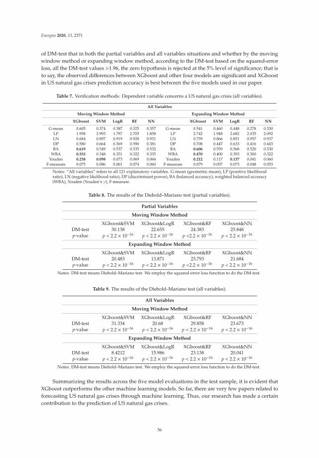
Energies 2020, 13, 2371

of DM-test that in both the partial variables and all variables situations and whether by the movingwindow method or expanding window method, according to the DM-test based on the squared-errorloss, all the DM-test values >1.96, the zero hypothesis is rejected at the 5% level of significance; that isto say, the observed differences between XGboost and other four models are significant and XGboostin US natural gas crises prediction accuracy is best between the five models used in our paper.

Table 7. Verification methods: Dependent variable concerns a US natural gas crisis (all variables).

All Variables


XGboost SVM LogR RF NN XGboost SVM LogR RF NN

G-mean 0.605 0.374 0.387 0.325 0.357 G-mean 0.541 0.460 0.448 0.278 0.330LP 1.958 2.993 1.797 2.705 1.858 LP 2.742 1.948 2.682 2.035 2.092LN 0.684 0.897 0.919 0.928 0.931 LN 0.759 0.866 0.851 0.957 0.937DP 0.580 0.664 0.369 0.590 0.381 DP 0.708 0.447 0.633 0.416 0.443BA 0.619 0.549 0.537 0.535 0.532 BA 0.606 0.559 0.568 0.520 0.530

WBA 0.553 0.348 0.351 0.322 0.335 WBA 0.470 0.400 0.393 0.300 0.322Youden 0.238 0.098 0.073 0.069 0.064 Youden 0.212 0.117 0.137 0.041 0.060

F-measure 0.075 0.086 0.061 0.074 0.060 F-measure 0.079 0.057 0.073 0.048 0.053

Notes: “All variables” refers to all 121 explanatory variables. G-mean (geometric mean), LP (positive likelihoodratio), LN (negative likelihood ratio), DP (discriminant power), BA (balanced accuracy), weighted balanced accuracy(WBA), Youden (Youden’s γ), F-measure.

Table 8. The results of the Diebold–Mariano test (partial variables).

Partial Variables

Moving Window Method

XGboost&SVM XGboost&LogR XGboost&RF XGboost&NNDM-test 30.138 22.655 24.383 25.848p-value p < 2.2 × 10−16 p < 2.2 × 10−16 p <2.2 × 10−16 p < 2.2 × 10−16

Expanding Window Method

XGboost&SVM XGboost&LogR XGboost&RF XGboost&NNDM-test 20.483 13.871 23.793 21.684p-value p < 2.2 × 10−16 p < 2.2 × 10−16 p <2.2 × 10−16 p < 2.2 × 10−16

Notes: DM-test means Diebold–Mariano test. We employ the squared-error loss function to do the DM-test.

Table 9. The results of the Diebold–Mariano test (all variables).

All Variables

Moving Window Method

XGboost&SVM XGboost&LogR XGboost&RF XGboost&NNDM-test 31.334 20.68 29.858 23.673p-value p < 2.2 × 10−16 p < 2.2 × 10−16 p < 2.2 × 10−16 p < 2.2 × 10−16

Expanding Window Method

XGboost&SVM XGboost&LogR XGboost&RF XGboost&NNDM-test 8.4212 15.986 23.138 20.041p-value p < 2.2 × 10−16 p < 2.2 × 10−16 p < 2.2 × 10−16 p < 2.2 × 10−16

Notes: DM-test means Diebold–Mariano test. We employ the squared-error loss function to do the DM-test.

Summarizing the results across the five model evaluations in the test sample, it is evident thatXGboost outperforms the other machine learning models. So far, there are very few papers related toforecasting US natural gas crises through machine learning. Thus, our research has made a certaincontribution to the prediction of US natural gas crises.

56

Energies 2020, 13, 2371

5.3. Confusion Matrix Results

Referring to Chatzis et al. [23], we computed the final classification performance confusionmatrices for the evaluated machine learning models (see Tables 10 and 11). Here, a false alarm meansa false positive rate, and the hit rate denotes the proportion of correct crisis predictions in the totalnumber of crises. For the best performing model, XGboost, we found that the false alarms do notexceed 25%, and the highest hit rate is 49%. Thus, our US natural gas crisis prediction accuracy canreach 49% using all variables with the moving window method.

Table 10. Confusion matrix results: Partial variables.

Partial Variables


XGboost Predict PredictTRUE 0 1 Signal TRUE 0 1 Signal

0 4103 934 False alarm 19% 0 4360 699 False alarm 15%

1 58 51 Hit rate 47% 1 52 35 Hit rate 40%

SVM Predict PredictTRUE 0 1 Signal TRUE 0 1 Signal

0 4895 142 False alarm 5% 0 4834 225 False alarm 6%1 95 14 Hit rate 13% 1 71 16 Hit rate 18%

LogR Predict PredictTRUE 0 1 Signal TRUE 0 1 Signal


RF Predict PredictTRUE 0 1 Signal TRUE 0 1 Signal


NN Predict PredictTRUE 0 1 Signal TRUE 0 1 Signal


Table 11. Confusion matrix results: All variables.

All Variables


XGboost Predict PredictTRUE 0 1 Signal TRUE 0 1 Signal

0 3786 1251 False alarm 25% 0 4444 615 False alarm 13%

1 56 53 Hit rate 49% 1 58 29 Hit rate 33%

SVM Predict PredictTRUE 0 1 Signal TRUE 0 1 Signal


LogR Predict PredictTRUE 0 1 Signal TRUE 0 1 Signal


RF Predict PredictTRUE 0 1 Signal TRUE 0 1 Signal


NN Predict PredictTRUE 0 1 Signal TRUE 0 1 Signal


57

Energies 2020, 13, 2371

6. Conclusions

We proposed a dynamic moving window and expanding window method that combines XGboost,an SVM, a LogR, an RF, and an NN as machine learning techniques to predict US natural gas crises.We proposed the following full procedure. First, we selected the most significant US natural gasfinancial market indicators, which we believe can be employed to predict US natural gas crises.Second, we combined the aforementioned dynamic methods with other methods (e.g., the returns andlags of the raw prices) to process the daily data set, and defined a crisis for the machine learning model.Third, we used the five machine learning models (XGboost, SVM, LogR, RF, and NN) with dynamicmethods to forecast the crisis events. Finally, we evaluated the performance of each model using variousvalidation measures. We demonstrated that combining dynamic methods with machine learningmodels can achieve a better performance in terms of predicting US natural gas crises. In addition,our empirical results indicated that XGboost with the moving window method achieves a goodperformance in predicting such crises.

Our main conclusions can be summarized as follows. From the various verification methods,DM-test results, and confusion matrix results, XGboost with a moving window approach achieveda good performance in predicting US natural gas crises, particularly in the partial variables case.In addition, LogR in the moving window method and NN in the expanding window method did notperform badly in the partial variables situation whereas SVM in the moving window and LogR inthe expanding window did not perform badly in the all variables situation. Our conclusions can helpus to forecast the crises of the US natural gas market more accurately. Because financial markets arecontagious, policymakers must consider the potential effect of a third market. This is equally importantfor asset management investors, because diversified benefits may no longer exist during volatile times.Therefore, these findings can help investors and policymakers detect crises, and thus take preemptiveactions to minimize potential losses.

The novel contributions of our study can be summarized as follows. First, to the best of ourknowledge, this study is the first to combine dynamic methodologies with machine learning to predictUS natural gas crises. A lot of the previous studies are about the currency exchange crises, bank creditcrises, and so on. So far, there are very few papers related to forecasting US natural gas crises throughmachine learning. Second, we implemented XGboost, a popular and advanced machine learning modelin the financial crisis prediction field. Additionally, we found that XGboost outperforms in forecastingUS natural gas crises. Third, we employed various parameter tuning methods (e.g., the grid-search) toimprove the prediction accuracy. Fourth, we used novel evaluation methods appropriate for imbalanceddata sets to measure the model performance and we also employed the DM-test method and foundthat the forecasting performance of XGboost is significant. Finally, we employed in-depth explanatoryvariables that cover the spectrum of major financial markets.

Before combining the dynamic methodologies with machine learning techniques, we performedordinary machine learning, in that 70% of the data was used as training data and 30% was used astest data. However, the prediction performance of this method was not so satisfactory. Althoughour research is the first to combine machine learning techniques with dynamic methodologies for USnatural gas crisis prediction, the prediction accuracy of our model can be improved. This is left tofuture research. Lastly, because economic conditions change continuously and crises continue to occur,predicting crisis events will remain an open research issue.

Author Contributions: Investigation, W.Z.; writing—original draft preparation, W.Z.; writing—review andediting, S.H.; project administration, S.H.; funding acquisition, S.H. All authors have read and agreed to thepublished version of the manuscript.




58

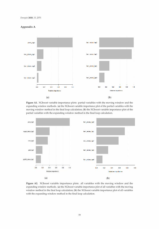
Energies 2020, 13, 2371

Appendix A

(a) (b)

Figure A1. XGboost variable importance plots: partial variables with the moving window and theexpanding window methods. (a) the XGboost variable importance plot of the partial variables with themoving window method in the final loop calculation; (b) the XGboost variable importance plot of thepartial variables with the expanding window method in the final loop calculation.

(a) (b)

Figure A2. XGboost variable importance plots: all variables with the moving window and theexpanding window methods. (a) the XGboost variable importance plot of all variables with the movingwindow method in the final loop calculation; (b) the XGboost variable importance plot of all variableswith the expanding window method in the final loop calculation.

59

Energies 2020, 13, 2371

(a)

(b)

Figure A3. Parameter tuning for the postulated SVM plot: partial variables with the moving windowand expanding window methods. (a) parameter tuning for the SVM plot of the partial variables withthe moving window method in the final loop calculation; (b) parameter tuning for the SVM plot of thepartial variables with the expanding window method in the final loop calculation.

(a) (b)

Figure A4. Parameter tuning for the postulated SVM plot: all variables with the moving windowand the expanding window methods. (a) parameter tuning for the SVM plot of all variables with themoving window method in the final loop calculation; (b) parameter tuning for the SVM plot of allvariables with the expanding window method in the final loop calculation.

60

Energies 2020, 13, 2371

(a) (b)

Figure A5. RF variable importance plots: partial variables with the moving window and the expandingwindow methods. (a) RF variable importance plot of the partial variables with the moving windowmethod in the final loop calculation; (b) RF variable importance plot of the partial variables with theexpanding window method in the final loop calculation.

(a) (b)

Figure A6. RF variable importance plots: all variables with the moving window and the expandingwindow methods. (a) RF variable importance plot of all variables with the moving window method inthe final loop calculation; (b) RF variable importance plot of all variables with the expanding windowmethod in the final loop calculation.

61

Energies 2020, 13, 2371

Table A1. Estimated LogR model result: Partial variables.

Partial Variables


Estimate Std. Error z-Value Pr(>|z|) Estimate Std. Error z-Value Pr(>|z|)

(Intercept) −7.91 1.19 −6.65 2.91 × 10−11 *** (Intercept) −1.88 × 103 1.12 × 106 −0.002 0.999crisis_ave5days 2.77 6.50 0.43 0.6698 crisis_ave5days −8.71 × 102 7.42 × 105 −0.001 0.999

crisis_lag1 2.61 1.56 1.67 0.0942 crisis_lag1 2.19 × 102 1.23 × 105 0.002 0.999hen_return_lag1 39.25 18.85 2.08 0.0373 * hen_return_lag1 2.90 × 103 1.31 × 106 0.002 0.998

Notes: *** < 0.001 p-value; * < 0.05 p-value.

Table A2. Estimated LogR model result: All variables.

All Variables


Estimate Std. Error z-Value Pr(>|z|) Estimate Std. Error z-Value Pr(>|z|)

(Intercept) −4.56 0.21 −21.87 2 × 10−16 *** (Intercept) −5.48 1.73 −3.17 0.00153 **crisis_ave5days 8.75 2.34 3.73 0.000190 *** crisis_ave5days 7.30 2.58 2.83 0.00465 **hen_return_lag5 7.31 2.21 3.31 0.000944 *** hen_return_lag5 6.60 2.39 2.76 0.00582 **hen_return_lag2 9.19 4.07 2.26 0.023885 * gold_return_lag5 2.61 9.88 2.64 0.00835 **

Notes: *** < 0.001 p-value; ** < 0.01 p-value; * < 0.05 p-value.

References

1. Birol, F. The Impact of the Financial and Economic Crisis on Global Energy Investments. In Proceedings ofthe Energy, Policies and Technologies for Sustainable Economies, IAEE (International Association for EnergyEconomics) European Conference, Vienna, Italy, 7–10 September 2009.

2. Klopotan, I.; Zoroja, J.; Mesko, M. Early warning system in business, finance, and economics: Bibliometricand topic analysis. Int. J. Eng. Bus. Manag. 2018, 10, 1–12. [CrossRef]

3. Edison, J.H. Do indicators of financial crises work? An evaluation of an early warning system. Int. J.Financ. Econ. 2003, 8, 11–53. [CrossRef]

4. Kaminsky, L.G.; Lizondo, S.; Reinhart, M.C. Leading indicators of currency crises. IMF Econ. Rev. 1998,45, 1–48. [CrossRef]

5. Kaminsky, L.G.; Reinhart, M.C. The twin crises: The causes of banking and balance-of-payments problems.Am. Econ. Rev. 1999, 89, 473–500. [CrossRef]

6. Lin, W.Y.; Hu, Y.H.; Tsai, C.F. Machine learning in financial crisis prediction: A survey. IEEE Trans. Syst.Man. Cybern. Part C 2012, 42, 421–436.

7. Chen, S.W.C.; Gerlach, R.; Lin, M.H.E.; Lee, W.C.W. Bayesian forecasting for financial risk management,pre and post the global financial crisis. J. Forecast. 2012, 31, 661–687. [CrossRef]

8. Bagheri, A.; Peyhani, M.H.; Akbari, M. Financial forecasting using ANFIS networks with quantum-behavedparticle swarm optimization. Expert Syst. Appl. 2014, 41, 6235–6250. [CrossRef]

9. Niemira, P.M.; Saaty, L.T. An analytic network process model for financial-crisis forecasting. Int. J. Forecast.2004, 20, 573–587. [CrossRef]

10. Chiang, W.C.; Enke, D.; Wu, T.; Wang, R.Z. An adaptive stock index trading decision support system.Expert Syst. Appl. 2016, 59, 195–207. [CrossRef]

11. Gorucu, B.F. Artificial neural network modeling for forecasting gas consumption. Energy Source 2004, 26,299–307. [CrossRef]

12. Xie, W.; Yu, L.; Xu, S.Y.; Wang, S.Y. A New Method for Crude Oil Price Forecasting Based on Support VectorMachines. In International Conference on Computational Science; Springer: Berlin/Heidelberg, Germany, 2006;pp. 444–451.

13. Frankel, A.J.; Rose, K.A. Currency crashes in emerging markets: An empirical treatment. J. Int. Econ. 1996,41, 351–366. [CrossRef]

14. Bae, K.H.; Karolyi, A.; Stulz, M.R. A new approach to measuring financial contagion. Rev. Financ. Stud. 2003,16, 717–763. [CrossRef]

15. Sachs, J.; Tornell, A.; Velasco, A. Financial crises in emerging markets: The lessons from 1995. Brook. Pap.Econ. Act. 1996, 27, 147–199. [CrossRef]

62

Energies 2020, 13, 2371

16. Knedlik, T.; Schweinitz, V.G. Macroeconomic imbalances as indicators for debt crises in Europe. J. CommonMarket Stud. 2012, 50, 726–745. [CrossRef]

17. Bussiere, M.; Fratzscher, M. Towards a new early warning system of financial crises. J. Int. Money Financ.2006, 25, 953–973. [CrossRef]

18. Xu, L.; Kinkyo, T.; Hamori, S. Predicting currency crises: A novel approach combining random forests andwavelet transform. J. Risk Financ. Manag. 2018, 11, 86. [CrossRef]

19. Saleh, N.; Casu, B.; Clare, A. Towards a new model for early warning signals for systemic financial fragilityand near crises: An application to OECD. Econom. Econom. Model Constr. Estim. Sel. J. 2012. [CrossRef]

20. Ahn, J.J.; Oh, K.J.; Kim, T.Y.; Kim, D.H. Usefulness of support vector machine to develop an early warningsystem for financial crisis. Expert Syst. Appl. 2011, 38, 2966–2973. [CrossRef]

21. Sevim, C.; Oztekin, A.; Bali, O.; Gumus, S.; Guresen, E. Developing an early warning system to predictcurrency crises. Eur. J. Oper. Res. 2014, 237, 1095–1104. [CrossRef]

22. Lin, C.S.; Khan, A.H.; Chang, R.Y.; Wang, Y.C. A new approach to modeling early warning systemsfor currency crises: Can a machine-learning fuzzy expert system predict the currency crises effectively?J. Int. Money Financ. 2008, 27, 1098–1121. [CrossRef]

23. Chatzis, P.S.; Siakoulis, V.; Petropoulos, A.; Stavroulakis, E.; Vlachogiannakis, N. Forecasting stock marketcrisis events using deep and statistical machine learning techniques. Expert Syst. Appl. 2018, 112, 353–371.[CrossRef]

24. Bolbol, A.; Cheng, T.; Tsapakis, I.; Haworth, J. Inferring hybrid transportation modes from sparse GPS datausing a moving window SVM classification. Comput. Environ. Urban Syst. 2012, 36, 526–537. [CrossRef]

25. Chou, J.S.; Ngo, N.T. Time series analytics using sliding window metaheuristic optimization-based machinelearning system for identifying building energy consumption patterns. Appl. Energy 2016, 177, 751–770.[CrossRef]

26. Oh, K.J.; Kim, T.Y.; Kim, C. An early warning system for detection of financial crisis using financial marketvolatility. Expert Syst. 2006, 23, 63–125. [CrossRef]

27. Patel, A.S.; Sarkar, A. Crises in developed and emerging stock markets. Financ. Anal. J. 1998, 54, 50–61.[CrossRef]

28. Coudert, V.; Gex, M. Does risk aversion drive financial crises? Testing the predictive power of empiricalindicators. J. Empir. Financ. 2008, 15, 167–184. [CrossRef]

29. Li, W.X.; Chen, C.S.C.; French, J.J. Toward an early warning system of financial crises: What can index futuresand options tell us? Q. Rev. Econ. Financ. 2015, 55, 87–99. [CrossRef]

30. Chen, T.Q.; He, T. xgboost: eXtreme Gradient Boosting. 2019. Available online: http://cran.fhcrc.org/web/packages/xgboost/vignettes/xgboost.pdf (accessed on 1 November 2019).

31. Vapnik, V.N. An overview of statistical learning theory. IEEE Trans. Neural Netw. 1999, 10, 988–999. [CrossRef]32. Ohlson, J. Financial ratios and the probabilistic prediction of bankruptcy. J. Account. Res. 1980, 18, 109–131.

[CrossRef]33. Breiman, L. Random forests. Mach. Learn. 2001, 45, 5–32. [CrossRef]34. Tanaka, K.; Kinkyo, T.; Hamori, S. Random Forests-based Early Warning System for Bank Failures. Econ. Lett.

2016, 148, 118–121. [CrossRef]35. Tanaka, K.; Higashide, T.; Kinkyo, T.; Hamori, S. Analyzing industry-level vulnerability by predicting

financial bankruptcy. Econ. Inq. 2019, 57, 2017–2034. [CrossRef]36. Werbos, P.J. Advanced forecasting methods for global crisis warning and models of intelligence.

Gen. Syst. Yearb. 1977, 22, 25–38.37. Friedman, J.H. Greedy function approximation: A gradient boosting machine. Ann. Stat. 2001, 29, 1189–1232.

[CrossRef]38. Erdogen, E.B. Prediction of bankruptcy using support vector machines: An application to bank bankruptcy.

J. Stat. Comput. Sim. 2012, 83, 1543–1555. [CrossRef]39. Yap, F.C.B.; Munuswamy, S.; Mohamed, B.Z. Evaluating company failure in Malaysia using financial ratios

and logistic regression. Asian J. Financ. Account. 2012, 4, 330–344. [CrossRef]40. Hothorn, T.; Everitt, B.S. A Handbook of Statistical Analyses Using R, 3rd ed.; CRC Press: Boca Raton,

FL, USA, 2014.41. Ho, T.K. Random decision forests. In Proceedings of the Third International Conference on Document

Analysis and Recognition, Montreal, QC, Canada, 14–16 August 1995; Volume 1, pp. 278–282.

63

Energies 2020, 13, 2371

42. Bekkar, M.; Djemaa, K.H.; Alitouche, A.T. Evaluation measures for models assessment over imbalanced datasets. J. Inf. Eng. Appl. 2013, 3, 27–38.

43. Powers, D.M. Evaluation: From precision, recall and fmeasure to roc, informedness, markedness andcorrelation. J. Mach. Learn. Technol. 2011, 2, 37–63.

44. Diebold, F.X.; Mariano, R. Comparing predictive accuracy. J. Bus. Econ. Stat. 1995, 13, 253–265.


64

energies

Article

Influence of Fluctuations in Fossil Fuel Commoditieson Electricity Markets: Evidence from Spot andFutures Markets in Europe

Tiantian Liu 1, Xie He 1, Tadahiro Nakajima 1,2 and Shigeyuki Hamori 1,*

1 Graduate School of Economics, Kobe University, Kobe 657-8501, Japan; [email protected] (T.L.);[email protected] (X.H.); [email protected] (T.N.)

2 The Kansai Electric Power Company, Incorporated, Osaka 530-8270, Japan* Correspondence: [email protected]; Tel.: +81-78-657-8501

Received: 4 March 2020; Accepted: 11 April 2020; Published: 13 April 2020

Abstract: Using a fresh empirical approach to time-frequency domain frameworks, this studyanalyzes the return and volatility spillovers from fossil fuel markets (coal, natural gas, and crude oil)to electricity spot and futures markets in Europe. In the time domain, by an approach developedby Diebold and Yilmaz (2012) which can analyze the directional spillover effect across differentmarkets, we find natural gas has the highest return spillover effect on electricity markets followedby coal and oil. We also find that return spillovers increase with the length of the delivery periodof electricity futures. In the frequency domain, using the methodology proposed by Barunik andKrehlik (2018) that can decompose the spillover effect into different frequency bands, we find most ofthe return spillovers from fossil fuels to electricity are produced in the short term while most of thevolatility spillovers are generated in the long term. Additionally, dynamic return spillovers havepatterns corresponding to the use of natural gas for electricity generation, while volatility spilloversare sensitive to extreme financial events.

Keywords: electricity; crude oil; natural gas; coal; spillover effects

1. Introduction

Electricity is traded in both spot and futures markets. Extensive research has been undertaken overthe past two decades concerning the spot market for electricity (e.g., [1–4]). Electricity is a non-storablegood and faces generation constraints, transmission constraints, and seasonal issues, which can causea timing imbalance in trade and fluctuations in electricity prices in the spot market.

Electricity futures have often played two roles for investors. First, electricity futures are anessential indicator to predict future spot prices. Second, electricity futures provide investors who arewilling to take positions in power markets an excellent risk management tool for reducing their riskexposure, by reducing the operational risks caused by high volatility in the electricity spot market. Forthis reason, electricity futures trading is more extensive than spot trading. There are also many studiesconcerning the electricity futures market (e.g., [5–8]).

Approximately half of the world’s electricity is generated by fossil fuels such as crude oil, naturalgas, and coal. According to the BP Statistical Review of World Energy 2019 [9], in 2018, approximately40.5% of electricity was produced by oil, gas, and coal sources in Europe, which also necessarily impliesthe possibility of the spillover effects across the fossil fuel markets and electricity market. Additionally,in Huisman and Kilic’s [5] study, they state that although electricity cannot be stored directly, it canbe stored in the sense that fossil fuels are storable. The electricity producer who wants to sell anelectricity futures contract can either purchase the amount of fossil fuels in the spot market and store ituntil the delivery period to fulfill the delivery agreement or purchase the fossil fuel futures instead of


Energies 2020, 13, 1900

storing them directly. For this reason, the price of electricity futures may be related to the storage costof fossil fuels. On the other hand, in electricity spot market, according to the Mosquera-López andNursimulu’s [10] research, unlike futures markets, the electricity spot prices are more determined byrenewable energy infeed and electricity demand but not the price of fossil fuels such as natural gas,coal, and carbon. Thus, our research aims to examine if there are some difference in the spillover effectsof fossil fuel commodity markets on the electricity market and futures in Europe. Additionally, giventhat there are many types of electricity futures contracts in terms of their delivery periods, we furtherexamine whether there are different spillover effects between fossil fuel commodities and electricityfutures with monthly, quarterly, and yearly delivery periods. To the best of our knowledge, althoughthere are several papers discussing the relationship between the fossil fuels and electricity futuresmarket, the relationship between fossil fuels and the price of electricity futures with different deliveryperiods have not been studied in previous research yet. However, it will help electricity marketinvestors to fully understand the information transmission between electricity markets and fossil fuelmarkets to make their portfolio optimization and hedge strategy better and more comprehensive.

Many studies have investigated the interdependent relationship between fossil fuel commoditiesand electricity markets. For example, Emery and Liu [11] studied the relationship between the prices ofelectricity futures and natural gas futures and found a cointegration between California–Oregon Borderand Palo Verde electricity futures and natural gas futures. Mjelde and Bessler [12] used a vector errorcorrection model to analyze the relationship between electricity spot prices and electricity-generatingfuel sources (natural gas, crude oil, coal, and uranium) in the US. The authors found that the peakelectricity price influences the natural gas price in contemporaneous time, while in the long term, apartfrom uranium, fuel source prices affect the electricity price. Based on the VECM model, Furió andChuliá [13] analyzed the volatility and price linkages between the Spanish electricity market, Brentcrude oil, and Zeebrugge (Belgium) natural gas. Natural gas and crude oil were seen to have anessential influence in the Spanish electricity market, with particular causality from the fossil fuel (Brentcrude oil and Zeebrugge natural gas) markets to the Spanish electricity forward market.

Generalized autoregressive conditional heteroskedasticity (GARCH)-type models have also beenused to study the relationship between electricity and fossil fuel markets. Serletis and Shahmoradi [14]used the GARCH-M model to investigate the linkages between natural gas and electricity prices andvolatilities in Alberta, Canada, and found a bidirectional causality. Using the BEKK-GARCH model,Green et al. [15] measured the strength of volatility spillovers in the electricity market in Germanycaused by volatility in natural gas, coal, and carbon emission markets. According to the results, duringthe sample period, natural gas and coal produced non-negligible spillovers while carbon emissionmarkets caused spillover effects from 2011 to 2014.

The return spillover is defined as the cross-market correlation between price changes (returns)allowing for one market’s price fluctuation to affect the other market’s direction with a lag. On theother hand, the volatility spillover could capture the correlation between the size of price changes.That is, if one market becomes riskier over a period of time (which implies bigger price fluctuations)the riskiness of the interrelated market will also change. Measuring the return spillover could allowinvestors to evaluate the investment trends of markets while measuring the volatility spillover couldenable investors to evaluate the risk information across markets. The information across marketsprovide useful insights into the portfolio diversification of investment, hedging strategies, and riskmanagement for financial agents.

In this study, we analyze the return and volatility spillovers from the fossil fuel market commoditiesof natural gas, coal, and crude oil, to electricity spot and futures markets in Europe, by using twonew empirical methods in the time-frequency domain: (1) the Diebold–Yilmaz approach; and (2)the Barunik and Krehlik methodology. The Diebold–Yilmaz approach was proposed in Diebold andYilmaz [16] and developed in Diebold and Yilmaz [17]. In the Diebold–Yilmaz approach, the spilloverindex can be constructed based on the variance decomposition of forecast error, which allows for thestudy of the spillover effect with a fixed investment horizon in a quantitative way. However, investors

66

Energies 2020, 13, 1900

have to consider different investment horizons when they make investment decisions because shocksmay have different effects in the short and long term. For this reason, Barunik and Krehlik [18] usedthe Fourier transform to convert the Diebold–Yilmaz approach into the frequency domain so thatthe spillover index could be decomposed at different frequencies. Moreover, we can also obtain thetime-varying spillover effect by using the moving window method. Many recent studies have usedthis method to study spillover effects and connectedness between assets, such as Singh et al. [19],Kang and Lee [20], and Malik and Umar [21]. In a more recent study, Lovcha and Perez-Laborda [22]used the Diebold–Yilmaz approach and the Barunik and Krehlik methodology to analyze the volatilityconnectedness between Henry Hub natural gas and West Texas Intermediate (WTI) crude oil in thetime and frequency domains. Lau et al. [23] used the E-GARCH model and the Barunik and Krehlikmethodology approach to investigate the return and volatility spillover effects among white preciousmetals, gold, oil, and global equity.

The remainder of this paper is structured as follows: Section 2 introduces the empirical methodused in this research, while Section 3 introduces the data used and preliminary analysis. Section 4explains and analyzes the empirical results, and Section 5 presents the conclusions.

2. Method Framework

Diebold and Yilmaz [17] proposed an approach for measuring spillover in the generalized vectorautoregression framework using the concept of connectedness, which built on the generalized forecasterror variance decomposition (GFEVD) of a Vector Autoregressive (VAR) model with p lags.

yt =

p∑i=1

Φiyt−i + εt, (1)

where yt is an N × 1 vector of observed variables at time t, Φ is the N × N coefficient matrices, anderror vector εt i.i.d ∼ (0, Σ) with covariance matrix Σ is possibly non-diagonal.

The VAR process can also be represented as the following Moving Average (∞) representationEquation (2), assuming the roots of

∣∣∣Φ(z)∣∣∣ lie outside the unit-circle:

yt = Ψ(L)εt, (2)

where Ψ(L) is an N × N coefficient matrix of infinite lag polynomials. Since the order of variables inthe VAR system may have an influence on the impulse response or variance decomposition results,Diebold and Yilmaz [17] modified the generalized VAR framework of Koop et al. [24] and Pesaran andShin [25] to ensure the variance decomposition’s independence of ordering. Under such a framework,the H-step-ahead generalized forecast error variance decomposition (GFEVD) can be presented in theform of Equation (3):

θHjk =

σ−1kk

∑Hh=0

((ΨhΣ) jk

)2

∑Hh=0

(ΨhΣΨ′

h

)j j

, (3)

where Ψh stands for an N × N coefficient matrix of polynomials at lag h, and σkk = (Σ)kk. The θHjk

represents H-steps ahead forecast error variance of the element j which is contributed by the k-thvariable of the VAR system. To make the sum of the elements in each row of the generalized forecasterror variance decomposition (GFEVD) equal to 1, each entry is standardized by the row sum as:

θHjk =

θHjk∑N

k=1 θHjk

, (4)

67

Energies 2020, 13, 1900

The θHjk is also defined as the Pairwise Spillover from k to j over the horizon H, which can measure

the spillover effect from market k to market j. Meanwhile, there are also directional spillovers asdefined by Diebold and Yilmaz:

Directional Spillovers (From): SHk←· = 100×

∑N

j = 1j � k

θHkj

N , the directional spillovers (From) measurethe spillovers from all other markets to market k.

The above-defined measures of spillovers are summarized in Table 1.

Table 1. The spillover table of the Diebold–Yilmaz approach (2012).

Spillover Results

y1 y2 . . . yN From othersy1 S1←1 S1←2 . . . S1←N SH

1←· =1N ΣN

j=1S1← j, j � 1

y2 S2←1 S2←2 . . . S2←N SH2←· =

1N ΣN

j=1S2← j, j � 2...

......

. . ....

...yN SN←1 SN←2 . . . SN←N SH

N←· =1N ΣN

j=1SN← j, j � N

Note: adapted from “On the Network Topology of Variance Decompositions: Measuring the Connectedness ofFinancial Firms” [26].

Barunik and Krehlik [1] proposed a methodology that could decompose the spillover index in theDiebold–Yilmaz approach on the specific frequency bands.

First and foremost, by the application of the Fourier transform, spillovers in the frequency domaincan be measured. Through a Fourier transform of the coefficients to obtain a frequency responsefunction Ψh: Ψ

(e−iω

)=∑

h e−iωhΨh, where i=√−1. The generalized causation spectrum over frequencies

ω ∈ (−π,π) can be defined as:

(f(ω)) jk ≡σ−1

kk

∣∣∣∣∣(Ψ(e−iω

)Σ)

jk

∣∣∣∣∣2(Ψ(e−iω)ΣΨ′(e+iω)) j j

(5)

It is crucial to note that (f(ω)) jk represents the contribution of the k-th variable to the portion ofthe spectrum of the j-th variable at a given frequency ω. To find the generalized decomposition ofvariance to different frequencies, (f(ω)) jk can be weighted by the frequency share of the variance ofthe j-th variable. The weighting function can be defined as:

Γ j(ω) =

(Ψ(e−iω

)ΣΨ′(e+iω

))j j

12π

∫ π−π(Ψ(e−iλ)ΣΨ′(e+iλ)) j jdλ

(6)

Equation (6) gives a presentation of the power of the j-th variable at a given frequency, the sumof the frequencies to a constant value of 2π. Meanwhile, it is important to note that the generalizedfactor spectrum is the squared coefficient of weighted complex numbers and is a real number when theFourier transform of the impulse is a complex number value. Therefore, we can set up the frequencyband d = (a,b): a, b∈ (−π,π), a < b.

The GFEVD under the frequency band d is:

θ jk(d) =1

2π

b∫a

Γ j(ω)(f(ω)) jkdω (7)

68

Energies 2020, 13, 1900

This also needs to be normalized; the scaled GFEVD on the frequency band d = (a,b): a, b∈ (−π,π),a < b can be defined as:

θ jk(d) =θ jk(d)∑k θ jk(∞)

(8)

We can define θ jk(d) as the pairwise spillover on a given frequency band d. Meanwhile, given thetotal spillover proposed by Diebold and Yilmaz [16], it is possible to define the total spillover on thefrequency band d. Similarly, there are also directional spillovers in the frequency domain:

Frequency Directional Spillovers (From): SFk←·(d) = 100×

∑N

j = 1j � k

θkj(d)

N , the frequency directionalspillovers (From) represents the spillovers from all other markets to market k on the frequency band d.

Similar to Table 1, the above-defined measures of spillovers on the frequency band d aresummarized in Table 2.

Table 2. The spillover table of the Barunik–Krehlik methodology (2018).

Spillover Results

y1 y2 . . . yN From othersy1 SF1←1(d) SF1←2(d) . . . SF1←N(d) SF1←·(d) =

1N ΣN

j=1SF1← j(d), j � 1

y2 SF2←1(d) SF2←2(d) . . . SF2←N(d) SF2←·(d) =1N ΣN

j=1SF2← j(d), j � 2...

......

. . ....

...yN SFN←1(d) SFN←2(d) . . . SFN←N(d) SFN←·(d) =

1N ΣN

j=1SFN← j(d), j � N

Note: adapted from “On the Network Topology of Variance Decompositions: Measuring the Connectedness ofFinancial Firms” [26].

3. Data and Preliminary Analysis

In this study, we use data from three fossil fuels markets: natural gas, coal, and crude oil; and fourelectricity markets: the electricity spot market and the monthly, quarterly, and yearly electricity futuresmarkets. We employ daily data for the period from 2 January 2007, to 2 January 2019, with a total of3019 observations. These data have been converted local currencies into euros at the daily exchangerate. All variables we used are listed in Table 3.



Ele_Spot EPEX Germany Baseload Spot BloombergEle_Fut_Mon EEX Germany Baseload Monthly Futures BloombergEle_Fut_Qr EEX Germany Baseload Quarterly Futures BloombergEle_Fut_Yr EEX Germany Baseload Yearly Futures BloombergGas ICE UK Natural Gas Monthly Futures BloombergCoal ICE Rotterdam Coal Monthly Futures BloombergOil ICE Brent Crude Oil Monthly Futures Bloomberg

For the fossil fuels markets, we used a representative price of natural gas, coal, and crude oilfutures markets in Europe. First, we used the United Kingdom (UK) National Balancing Point (NBP)natural gas futures to represent the natural gas market. The NBP natural gas market is the oldestnatural gas market in Europe and is widely used as a leading benchmark for the wholesale gas marketin Europe. Second, we used the Rotterdam coal futures to represent the coal market, which is financiallysettled based upon the price of coal delivered into the Amsterdam, Rotterdam, and Antwerp regions ofthe Netherlands. The futures contract is cash-settled against the API 2 Index, which is the benchmarkprice reference for coal imported to Northwest Europe. Third, we used the Brent crude oil futures to

69

Energies 2020, 13, 1900

represent the crude oil market. The Brent crude oil market is one of the world’s most liquid crude oilmarkets. The price of Brent crude oil is the benchmark for African, European, and Middle Easterncrude. All futures mentioned above are traded on the Intercontinental Exchange (ICE) Futures Europecommodities market. The price of natural gas quoted in EUR per therm, the price of coal quoted inEUR per metric ton, and the price of crude oil quoted in EUR per barrel.

In Europe, electricity futures markets are offered in the European Energy Exchange (EEX). The EEXis a central European electric power exchange established in August 2000 and has become the leadingenergy exchange in Europe with more than 200 trading participants from 19 countries. In 2008, thepower spot markets EEX and Powenext merged to create the European Power Exchange (EPEX SPOT)to offer spot markets in electricity. In this study, we used the spot, monthly futures, quarterly futures,and yearly futures markets of the Physical Electricity Index (Phelix) Baseload, which is the reference inGermany and majority of Europe. The electricity spot commodity is traded in the EPEX SPOT, andfutures commodities are traded in the EEX. The prices of electricity spot and futures quoted in EURper megawatt-hour (Mwh).

The closing prices of all variables are plotted in Figure 1. As shown, we find that the variation inelectricity spot prices is more extreme, with more spikes and jumps than other commodities. It is clearthat electricity futures and fossil fuel prices show a similar pattern.

In this study, we calculated the first order logged differences in prices as the returns and extractedthe conditional variance series by fitting the AR-GARCH model as the volatilities. The descriptivestatistics for the returns and volatilities of the variables are given in Table 4, where we can see, asexpected, that the electricity spot market is the most volatile. The skewness value of the return of coalfutures is negative and others are positive. Meanwhile, quarterly electricity futures have the highestskewness, indicating that they have the most extreme gains.

Table 4. Descriptive statistics of the return and volatility series.

Spot Fut_Mon Fut_Qr Fut_Yr Gas Coal Oil

Descriptive Statistics of the Return

Mean 0.0002 0.0000 0.0001 −0.0000 0.0001 0.0001 0.0000Minimum −2.0000 −0.2429 −0.2002 −0.09366 −0.1334 0.2179 −0.1094Maximum 2.3785 0.4042 0.3422 0.1535 0.3589 0.1751 0.1718Std. Dev. 0.2537 0.0315 0.0204 0.0118 0.0296 0.0161 0.0211Skewness 0.6253 2.415 3.1200 0.5691 1.8429 −0.4293 0.0590Kurtosis 11.4001 38.3887 72.8856 16.7734 22.1089 35.6286 7.3911

JB 9072.9 *** 160,472 *** 619,264 *** 24,026 *** 47,642 *** 134,014 *** 2427.2 ***ADF −56.9 *** −37.7 *** −36.9 *** −38.0 *** −39.8 *** −39.1 *** −39.9 ***PP −123.9 *** −52.1 *** −51.6 *** −50.9 *** −52.2 *** −53.2 *** −59.1 ***

Descriptive Statistics of the Volatility

Mean 0.0589 0.0010 0.0003 0.0001 0.0001 0.0003 0.0004Minimum 0.0160 0.0006 0.0000 0.0000 0.0009 0.0001 0.0001Maximum 0.9180 0.0020 0.0068 0.0023 0.0136 0.0018 0.0048Std. Dev. 0.0589 0.0003 0.0005 0.0002 0.0012 0.0002 0.0005

Skewnesss 5.3783 1.3262 6.3463 4.0463 4.0977 2.9271 3.5460Kurtosis 52.2126 4.0317 58.6978 30.5627 29.5249 12.4334 20.0091

JB 319,207 *** 1018.8 *** 410,502 *** 103,802 *** 96,952 *** 15,505 *** 42,720 ***ADF −9.7 *** −3.4 ** −10.3 *** −5.6 *** −7.0 *** −3.0 ** −3.5 ***PP −11.7 *** −3.3 ** −12.6 *** −7.8 *** −10.2 *** −3.3 ** −3.9 ***

Note: Spot, Fut_Mon, Fut_Qr, Fut_Yr, Gas, Coal, Oil refer to EPEX Germany Baseload Spot, EEX Germany BaseloadMonthly Futures, EEX Germany Baseload Quarterly Futures, EEX Germany Baseload Yearly Futures, ICE UKNatural Gas Monthly Futures, ICE Rotterdam Coal Monthly Futures, ICE Brent Crude Oil Monthly Futures,respectively. JB: Jarque and Bera Test (1980); ADF: Augmented Dickey and Fuller Unit Root Test (1979); PP: Phillipsand Perron Unit Root Test (1988); *, ** and *** denote rejection of the null hypothesis at 10%, 5% and 1% significancelevels, respectively.

70

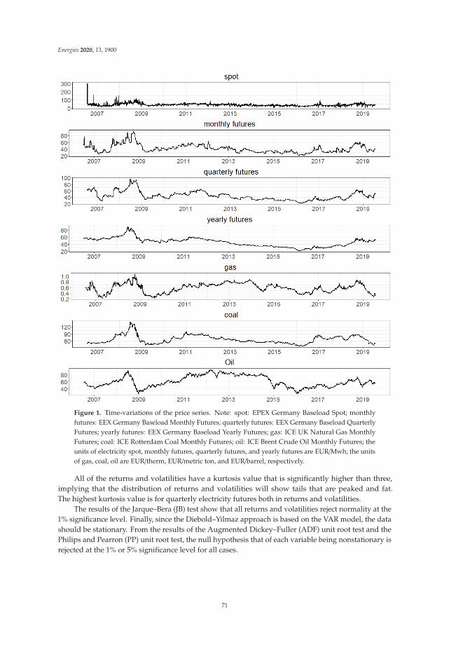
Energies 2020, 13, 1900

Figure 1. Time-variations of the price series. Note: spot: EPEX Germany Baseload Spot; monthlyfutures: EEX Germany Baseload Monthly Futures; quarterly futures: EEX Germany Baseload QuarterlyFutures; yearly futures: EEX Germany Baseload Yearly Futures; gas: ICE UK Natural Gas MonthlyFutures; coal: ICE Rotterdam Coal Monthly Futures; oil: ICE Brent Crude Oil Monthly Futures; theunits of electricity spot, monthly futures, quarterly futures, and yearly futures are EUR/Mwh; the unitsof gas, coal, oil are EUR/therm, EUR/metric ton, and EUR/barrel, respectively.

All of the returns and volatilities have a kurtosis value that is significantly higher than three,implying that the distribution of returns and volatilities will show tails that are peaked and fat.The highest kurtosis value is for quarterly electricity futures both in returns and volatilities.

The results of the Jarque–Bera (JB) test show that all returns and volatilities reject normality at the1% significance level. Finally, since the Diebold–Yilmaz approach is based on the VAR model, the datashould be stationary. From the results of the Augmented Dickey–Fuller (ADF) unit root test and thePhilips and Pearron (PP) unit root test, the null hypothesis that of each variable being nonstationary isrejected at the 1% or 5% significance level for all cases.

71

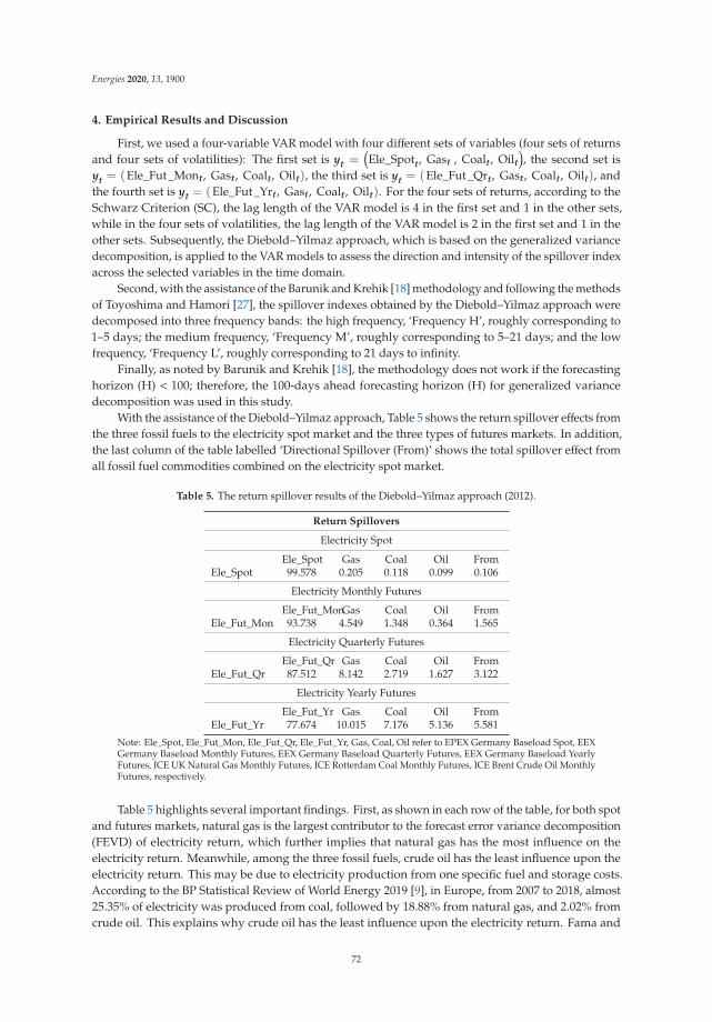
Energies 2020, 13, 1900

4. Empirical Results and Discussion

First, we used a four-variable VAR model with four different sets of variables (four sets of returnsand four sets of volatilities): The first set is yt =

(Ele_Spott, Gast , Coalt, Oilt

), the second set is

yt = (Ele_Fut_Mont, Gast, Coalt, Oilt), the third set is yt = (Ele_Fut_Qrt, Gast, Coalt, Oilt), andthe fourth set is yt = (Ele_Fut_Yrt, Gast, Coalt, Oilt). For the four sets of returns, according to theSchwarz Criterion (SC), the lag length of the VAR model is 4 in the first set and 1 in the other sets,while in the four sets of volatilities, the lag length of the VAR model is 2 in the first set and 1 in theother sets. Subsequently, the Diebold–Yilmaz approach, which is based on the generalized variancedecomposition, is applied to the VAR models to assess the direction and intensity of the spillover indexacross the selected variables in the time domain.

Second, with the assistance of the Barunik and Krehik [18] methodology and following the methodsof Toyoshima and Hamori [27], the spillover indexes obtained by the Diebold–Yilmaz approach weredecomposed into three frequency bands: the high frequency, ‘Frequency H’, roughly corresponding to1–5 days; the medium frequency, ‘Frequency M’, roughly corresponding to 5–21 days; and the lowfrequency, ‘Frequency L’, roughly corresponding to 21 days to infinity.

Finally, as noted by Barunik and Krehik [18], the methodology does not work if the forecastinghorizon (H) < 100; therefore, the 100-days ahead forecasting horizon (H) for generalized variancedecomposition was used in this study.

With the assistance of the Diebold–Yilmaz approach, Table 5 shows the return spillover effects fromthe three fossil fuels to the electricity spot market and the three types of futures markets. In addition,the last column of the table labelled ‘Directional Spillover (From)’ shows the total spillover effect fromall fossil fuel commodities combined on the electricity spot market.

Table 5. The return spillover results of the Diebold–Yilmaz approach (2012).

Return Spillovers

Electricity Spot

Ele_Spot Gas Coal Oil FromEle_Spot 99.578 0.205 0.118 0.099 0.106

Electricity Monthly Futures

Ele_Fut_MonGas Coal Oil FromEle_Fut_Mon 93.738 4.549 1.348 0.364 1.565

Electricity Quarterly Futures

Ele_Fut_Qr Gas Coal Oil FromEle_Fut_Qr 87.512 8.142 2.719 1.627 3.122

Electricity Yearly Futures

Ele_Fut_Yr Gas Coal Oil FromEle_Fut_Yr 77.674 10.015 7.176 5.136 5.581

Note: Ele_Spot, Ele_Fut_Mon, Ele_Fut_Qr, Ele_Fut_Yr, Gas, Coal, Oil refer to EPEX Germany Baseload Spot, EEXGermany Baseload Monthly Futures, EEX Germany Baseload Quarterly Futures, EEX Germany Baseload YearlyFutures, ICE UK Natural Gas Monthly Futures, ICE Rotterdam Coal Monthly Futures, ICE Brent Crude Oil MonthlyFutures, respectively.

Table 5 highlights several important findings. First, as shown in each row of the table, for both spotand futures markets, natural gas is the largest contributor to the forecast error variance decomposition(FEVD) of electricity return, which further implies that natural gas has the most influence on theelectricity return. Meanwhile, among the three fossil fuels, crude oil has the least influence upon theelectricity return. This may be due to electricity production from one specific fuel and storage costs.According to the BP Statistical Review of World Energy 2019 [9], in Europe, from 2007 to 2018, almost25.35% of electricity was produced from coal, followed by 18.88% from natural gas, and 2.02% fromcrude oil. This explains why crude oil has the least influence upon the electricity return. Fama and

72

Energies 2020, 13, 1900

French [28] state that a trader can offset the risk of positions they have in a forward contract by holdinga long or short inventory in the underlying commodity. Huisman and Kilic [5] note that althoughelectricity cannot (yet) be stored directly, it can be stored in the sense that fossil fuels are storable.When an electricity producer sells an electricity futures contract, they have two choices: (1) purchasethe amount of fossil fuels in the spot market and store it until the delivery period to fulfill the deliveryagreement or; (2) purchase the fossil fuel futures instead of storing them directly. If the fuels have ahigh storage cost, the electricity producers would prefer to hold a futures contract on the fuels ratherthan purchase them in the spot market and store them directly. Compared to coal and crude oil, naturalgas has higher storage costs and, therefore, the electricity producer would prefer to purchase naturalgas futures. This further explains the high connectedness of electricity and natural gas futures markets.Based on high demand and high storage costs, it is not difficult to understand why natural gas futureshave the most influence on the returns of electricity.

Second, it is interesting to note that the most significant return spillover effects are seen in yearlyelectricity futures, followed by the spillover effect to quarterly futures, then monthly futures. The returnspillovers from fossil fuel commodities is the least in the electricity spot market. Under the assumptionof storage costs mentioned earlier, when an electricity producer sells an electricity futures contract witha long delivery period, they would prefer to purchase futures contracts on underlying fuel commodities,rather than purchase them in the spot market and store until the delivery period. This implies thatthe return spillovers from fuel futures to electricity futures with a long delivery period are higherthan to electricity futures with a short delivery period. Mosquera-López and Nursimulu [10] exploredthe drivers of German electricity prices in spot and futures markets and found that spot prices aredetermined by renewable energy infeed and electricity demand, while in futures markets prices aredetermined by the price of fossil fuels such as natural gas, coal, and carbon. This may explain whythe return spillovers from fossil fuel commodities to electricity futures are higher than to electricityspot prices.

The return spillover results of Barunik and Krehil [16], which decompose the Diebold–Yilmazspillover indexes into three different frequencies, are presented in Table 6. The spillovers from fossilfuel commodities to electricity markets are highest in the high frequency, followed by the mediumfrequency and the low frequency. This indicates that return shocks are transmitted from fossil fuelmarkets to electricity markets within only one week.

Table 7 shows the volatility spillover effects from the threVe fossil fuel commodities to the electricityspot market and the three types of futures. The results are unusual; among the three fossil fuel markets,natural gas has the highest volatility spillovers to electricity spot markets (0.691%), monthly (9.539%),and quarterly futures (3.565%), but not to yearly futures (0.145%). Additionally, oil exhibits the weakestvolatility spillovers to all electricity markets (0.098%, 0.417%, and 0.211%, respectively), again, with theexception of yearly futures (1.835%).

In addition, in contrast to the return spillover results, the volatility spillovers from natural gasto monthly electricity futures (9.539%) is higher than for electricity futures with a longer deliveryperiod. However, crude oil and coal transmit the highest volatility spillovers to yearly futures, whilethe spillovers to monthly futures are higher than to quarterly futures. Finally, with the exception ofnatural gas, both volatility spillovers and return spillovers are higher for electricity futures than for theelectricity spot market.

Table 8 displays the volatility spillover results in the frequency domain. In contrast to the resultsin Table 6, the total volatility spillover is higher in the low frequency than in the high frequency.This indicates that the transmission of volatility shocks from fossil fuel markets to electricity markets isslower than that of return spillovers. The transmitted shocks from fossil fuels have long-lasting effectson electricity market volatility.

73

Energies 2020, 13, 1900

Table 6. The return spillover results of the Barunik–Krehlik methodology (2018).

Return Spillovers

Electricity Spot

Frequency H 1–5 DaysEle_Spot Gas Coal Oil From

Ele_Spot 97.182 0.193 0.116 0.084 0.098Frequency M 5–21 Days

Ele_Spot 1.902 0.009 0.002 0.011 0.005Frequency L > 21 Days

Ele_Spot 0.494 0.003 0.001 0.004 0.002


Frequency H 1–5 DaysEle_Fut_MonGas Coal Oil From

Ele_Fut_Mon 74.381 2.913 0.961 0.250 1.031Frequency M 5–21 DaysEle_Fut_Mon 14.234 1.191 0.283 0.083 0.389Frequency L > 21 DaysEle_Fut_Mon 5.123 0.445 0.104 0.031 0.145


Frequency H 1–5 DaysEle_Fut_QrGas Coal Oil From

Ele_Fut_Qr 68.856 5.671 1.974 1.149 2.199Frequency M 5–21 DaysEle_Fut_Qr 13.703 1.803 0.545 0.349 0.674Frequency L > 21 DaysEle_Fut_Qr 4.953 0.668 0.200 0.129 0.249


Frequency H 1–5 DaysEle_Fut_YrGas Coal Oil From

Ele_Fut_Yr 60.862 7.287 5.117 3.450 3.964Frequency M 5–21 DaysEle_Fut_Yr 12.348 1.993 1.505 1.231 1.182Frequency L > 21 DaysEle_Fut_Yr 4.464 0.734 0.553 0.455 0.436


Table 7. The volatility spillover results of the Diebold–Yilmaz approach (2012).

Volatility Spillovers

Electricity Spot

Ele_Spot Gas Coal Oil FromEle_Spot 98.804 0.691 0.407 0.098 0.299


Ele_Fut_Mon Gas Coal Oil FromEle_Fut_Mon 87.992 9.539 2.052 0.417 3.002


Ele_Fut_Qr Gas Coal Oil FromEle_Fut_Qr 95.585 3.565 0.639 0.211 1.104


Ele_Fut_Yr Gas Coal Oil FromEle_Fut_Yr 88.839 0.145 9.181 1.835 2.790


74

Energies 2020, 13, 1900

Table 8. The volatility spillover results of the Barunik–Krehlik methodology (2018).

Volatility Spillovers

Electricity Spot

Frequency H 1–5 DaysEle_Spot Gas Coal Oil From

Ele_Spot 9.671 0.003 0.003 0.002 0.002Frequency M 5–21 Days

Ele_Spot 35.053 0.042 0.009 0.010 0.015Frequency L > 21 Days

Ele_Spot 54.079 0.646 0.395 0.086 0.282


Frequency H 1–5 DaysEle_Fut_MonGas Coal Oil From

Ele_Fut_Mon 0.297 0.009 0.010 0.009 0.007Frequency M 5–21 DaysEle_Fut_Mon 0.852 0.029 0.029 0.026 0.021Frequency L > 21 DaysEle_Fut_Mon 86.843 9.502 2.012 0.382 2.974


Frequency H 1–5 DaysEle_Fut_QrGas Coal Oil From

Ele_Fut_Qr 9.962 0.195 0.000 0.014 0.052Frequency M 5–21 DaysEle_Fut_Qr 24.567 0.536 0.001 0.034 0.143Frequency L > 21 DaysEle_Fut_Qr 61.057 2.834 0.638 0.164 0.909


Frequency H 1–5 DaysEle_Fut_YrGas Coal Oil From

Ele_Fut_Yr 4.405 0.002 0.018 0.001 0.005Frequency M 5–21 DaysEle_Fut_Yr 11.985 0.005 0.050 0.003 0.015Frequency L > 21 DaysEle_Fut_Yr 72.448 0.138 9.113 1.831 2.771


It is well established that financial markets can be affected by extreme events such as financialcrises, price fluctuations, and market turmoil. For this reason, this section of our paper aims to capturethe dynamics of spillover, in particular to investigate how spillovers from the fossil fuel market to theelectricity market may change under extreme events. To accomplish this, a moving windows analysiswith a 400-day window length was applied.

Figure 2 presents the dynamic directional return spillover from all fossil fuel commoditiesto electricity markets, measured by the Diebold–Yilmaz approach (2012) and the Barunik–Krehlikmethodology (2018). The pairwise directional return spillovers are shown in Figure A1 in theAppendix A. In Figure 2, the solid line refers to the time-varying spillover of the Diebold–Yilmazapproach (2012), the long-dash line refers to spillover in the high frequency (1–5 days), the dotted linerefers to spillover in the medium frequency (5–21 days), and the two-dash line refers to spillover in thelow frequency (over 22 days). The results in Figure 2 indicate various characteristics.

First, the spillover effect of all three fossil fuel commodities to yearly electricity futures vary from0% to 8.7%, followed by quarterly futures (0% to 6.3%), monthly futures (0% to 5.8%), and the spotmarket (0% to 2.8%). According to the results, it can be concluded that the return spillovers from fossil

75

Energies 2020, 13, 1900

fuel commodities to electricity futures with a long delivery period are higher than to those with ashort delivery period and that the return spillover effect is lowest in the electricity spot market. This isconsistent with the results of the statistical analysis in Table 5.

Second, the spillovers from all three fossil fuel commodities to electricity markets are highest inthe high frequency category, followed by the medium frequency and low frequency categories. This isalso consistent with the results of the statistical analysis, shown in Table 6.

On the other hand, the proportion of spillovers from fossil fuel commodities to electricity futuresin the medium frequency and low frequency categories are higher than to the electricity spot market inthose frequencies. Compared to electricity spot, it appears that the spillovers to electricity futures arehigher in the long term. There is an implicit possibility that the speed of information transmissionfrom fossil fuel commodities to electricity futures is slower than to electricity spot.

Finally, it is clear that the patterns of return spillovers from fossil fuel commodities to electricityspot and futures markets are quite different. As we mentioned before, spot prices are determined byrenewable infeed and electricity demand while futures prices are determined by fossil fuels and mostlyinfluenced by natural gas. We find that the directional spillover from fossil fuel commodities to theelectricity futures market, especially quarterly futures and yearly futures, has some similar patternswith the change of electricity production toward natural gas in Europe. For example, the spillovers toquarterly and yearly futures decreased until 2015 but then tended to increase thereafter. This closelycorresponds with the changes in electricity production using natural gas in Europe, which decreasedfrom 2010 to 2015 and has since increased, as indicated by Figure 3.

Figure 2. Cont.

76

Energies 2020, 13, 1900

Figure 2. Diebold–Yilmaz approach (2012) directional return spillover (From) and Barunik–Krehlikmethodology (2018) directional return spillover (From). Note: spot: EPEX Germany Baseload Spot;monthly futures: EEX Germany Baseload Monthly Futures; quarterly futures: EEX Germany BaseloadQuarterly Futures; yearly futures: EEX Germany Baseload Yearly Futures.

-

200.0

400.0

600.0

800.0

1000.0

2009 2010 2011 2012 2013 2014 2015 2016 2017 2018

tera

wat

t-hou

r (Tw

h)

Figure 3. Electricity generation by natural gas in Europe. Data source: BP Statistical Review of WorldEnergy, 2019.

77

Energies 2020, 13, 1900

The findings regarding dynamic directional volatility spillover from all fossil fuel commoditiesto electricity markets are presented in Figure 4 (The pairwise directional volatility spillovers areshown in Figure 2 in the Appendix A). First, it appears that the volatility spillover evolves morefiercely in contrast to return spillovers. In particular, there are many sharp increases, or fluctuations,corresponding to extreme events. This further indicates that volatility spillovers may be more sensitiveto extreme events than return spillovers. For example, there are three significant sharp fluctuations in2009, 2015, and 2016, possibly influenced by the 2008 global financial crisis, the 2014 international oilprice’s violent shock, and the 2016 rise of coal and natural gas prices. Additionally, the proportions ofvolatility spillovers from fossil fuel commodities to electricity markets in the high frequency and lowfrequency categories also increased when the extreme events occurred.

Figure 4. Cont.

78

Energies 2020, 13, 1900

Figure 4. Diebold–Yilmaz approach (2012) directional volatility spillover (From) and Barunik–Krehlikmethodology (2018) directional volatility spillover (From). Note: spot: EPEX Germany Baseload Spot;monthly futures: EEX Germany Baseload Monthly Futures; quarterly futures: EEX Germany BaseloadQuarterly Futures; yearly futures: EEX Germany Baseload Yearly Futures.

Second, the volatility spillovers from all three fossil fuel commodities to electricity markets arehighest in the low frequency category, followed by medium frequency and then high frequency, whichis consistent with the results of the statistical analysis in Table 8.

5. Conclusions

This study analyzed return and volatility spillover effects from coal, natural gas, and crude oilfossil fuel markets to electricity spot and futures markets in Europe from 2 January 2007, to 2 January2019, using a new empirical method in the time-frequency domain frameworks developed by Dieboldand Yilmaz [17] and Barunik and Krehlik [18]. The study obtained the following major findings.

First, natural gas has the highest return spillover effect upon the electricity spot market and futuresmarkets, followed by coal and crude oil. The results may be explained by two factors: (1) electricityproduction favoring one specific fossil fuel and; (2) the different storage cost of fossil fuels.

Second, due to increasing storage costs over time, the return spillovers from fossil fuel commoditiesto electricity futures with a long delivery period are higher than to electricity futures with a short

79

Energies 2020, 13, 1900

delivery period. Meanwhile, compared to electricity futures markets, the spot market is more dependenton renewable energy infeed and electricity demand than fossil fuels such as natural gas and coal. Thus,the return spillover effect on electricity futures is higher than on electricity spot markets.

Third, in the frequency domain, we found that the majority of return spillover is generated inthe short term which further implies that return shocks are transmitted from fossil fuel markets toelectricity markets within only one week.

Contrary to expectations, we found that among the three fossil fuel markets, natural gas has thehighest volatility spillover effect on electricity spot markets and monthly and quarterly futures, but noton yearly futures. Similarly, oil exhibits the weakest volatility spillover effect on all electricity markets,also except yearly futures markets.

Additionally, the volatility spillover from natural gas to monthly electricity futures is higherthan for electricity futures with a longer delivery period. Meanwhile, crude oil and coal cause thehighest volatility spillovers to yearly electricity futures, followed by monthly and then quarterlyfutures. Except for natural gas, the volatility spillovers from coal and crude oil to electricity futuresare higher than in the electricity spot market, which is the same result as that found in the analysis ofreturn spillovers.

In the frequency domain, the majority of volatility spillover is produced in the long term whichfurther indicates that transmitted shocks from fluctuations in fossil fuels have long-lasting effects onelectricity market volatility.

Furthermore, we also explored dynamic spillovers by adopting the 400-day moving windowmethod. We found there is a similar pattern in the dynamics of return spillovers from fossil fuelcommodities to electricity futures with long delivery periods, and to electricity generation from naturalgas. However, we found the dynamic volatility spillovers from fossil fuels to electricity markets aremore sensitive to extreme events such as the 2008 global financial crisis, the 2014 international oilprice’s violent shock, and the 2016 rise in coal and natural gas prices, as shown by volatility spilloversvarying sharply when the extreme events occurred.

The results in this paper may be helpful for investors with different investment horizons inEurope to diversify their portfolios, hedge their strategies, and make their risk management plans.For short term investors, constructing well-diversified portfolios consisting of fossil fuels futures,electricity spot and futures is a complicated task, especially in times of financial turmoil. On theother hand, for long-term investors, including the fossil fuels in portfolios composed primarily ofelectricity spot and futures with different delivery periods could enable them to obtain the long-termdiversification benefits.

Author Contributions: Conceptualization, T.N. and S.H.; investigation, T.L. and X.H.; writing—original draftpreparation, T.L.; writing—review and editing, X.H., T.N., and S.H.; project administration, S.H.; fundingacquisition, S.H. All authors have read and agreed to the published version of the manuscript.

Funding: This work was supported by JSPS KAKENHI Grant Number 17H00983.

Acknowledgments: We are grateful to Keukwan Ryu and two anonymous referees for helpful commentsand suggestions.


80

Energies 2020, 13, 1900

Ap

pe

nd

ixA

F

igu

reA

1.

Die

bold

–Yilm

azap

proa

ch(2

012)

dire

ctio

nalr

etur

nsp

illov

er(P

airw

ise)

and

Baru

nik–

Kre

hlik

met

hodo

logy

(201

8)di

rect

iona

lret

urn

spill

over

(Pai

rwis

e).

81

Energies 2020, 13, 1900

F

igu

re2

.D

iebo

ld–Y

ilmaz

app

roac

h(2

012)

dir

ecti

onal

vola

tilit

ysp

illov

er(P

airw

ise)

and

Bar

uni

k–K

rehl

ikm

etho

dol

ogy

(201

8)d

irec

tion

alvo

lati

lity

spill

over

(Pai

rwis

e).

82

Energies 2020, 13, 1900

References

1. Bublitz, A.; Keles, D.; Fichtner, W. An analysis of the decline of electricity spot prices in Europe: Who is toblame? Energy Policy 2017, 107, 323–336. [CrossRef]

2. Kalantzis, F.G.; Milonas, N.T. Analyzing the impact of futures trading on spot price volatility: Evidence fromthe spot electricity market in France and Germany. Energy Econ. 2013, 36, 454–463. [CrossRef]

3. Menezes, L.M.; Houllier, M.A.; Tamvakis, M. Time-varying convergence in European electricity spot marketsand their association with carbon and fuel prices. Energy Policy 2016, 88, 613–627. [CrossRef]

4. Paschen, M. Dynamic analysis of the German day-ahead electricity spot market. Energy Econ. 2016, 59,118–128. [CrossRef]

5. Huisman, R.; Kilic, M. Electricity futures prices: Indirect storability, expectations, and risk Premiums. EnergyEcon. 2012, 34, 892–898. [CrossRef]

6. Islyaev, S.; Date, P. Electricity futures price models: Calibration and forecasting. Eur. J. Oper. Res. 2015, 247,144–154. [CrossRef]

7. Junttila, J.; Myllymäki, V.; Raatikainen, J. Pricing of electricity futures based on locational price differences:The case of Finland. Energy Econ. 2018, 71, 222–237. [CrossRef]

8. Kallabis, T.; Pape, C.; Weber, C. The plunge in German electricity futures prices Analysis using a parsimoniousfundamental model. Energy Policy 2016, 95, 280–290. [CrossRef]

9. BP Statistical Review of World Energy. Available online: https://www.bp.com/en/global/corporate/energy-economics/statistical-review-of-world-energy.html (accessed on 15 August 2019).

10. Mosquera-López, S.; Nursimulu, A. Drivers of electricity price dynamics: Comparative analysis of spot andfutures markets. Energy Policy 2019, 126, 76–87. [CrossRef]

11. Emery, G.W.; Liu, Q.F. An analysis of the relationship between electricity and natural-gas futures prices.J. Futures Mark. 2002, 22, 95–122. [CrossRef]

12. Mjelde, J.W.; Bessler, D.A. Market integration among electricity markets and their major fuel source markets.Energy Econ. 2009, 31, 482–491. [CrossRef]

13. Furió, D.; Chuliá, H. Price and volatility dynamics between electricity and fuel costs: Some evidence forSpain. Energy Econ. 2012, 34, 2058–2065. [CrossRef]

14. Serletis, A.; Shahmoradi, A. Measuring and Testing Natural Gas and Electricity Markets Volatility: Evidencefrom Alberta’s Deregulated Markets. Stud. Nonlinear Dyn. Econ. 2006, 10, 1–20. [CrossRef]

15. Green, R.; Larsson, K.; Lunina, V.; Nilsson, B. Cross-commodity news transmission and volatility spilloversin the German energy markets. Bank. Financ. 2018, 95, 231–243. [CrossRef]

16. Diebold, F.X.; Yilmaz, K. Measuring financial asset return and volatility spillovers, with application to globalequity markets. Econ. J. 2009, 119, 158–171. [CrossRef]

17. Diebold, F.X.; Yilmaz, K. Better to give than to receive: Forecast-based measurement of volatility spillovers.Int. J. Forecast. 2012, 28, 57–66. [CrossRef]

18. Baruník, J.; Krehlík, T. Measuring the frequency dynamics of financial connectedness and systemic risk.J. Financ. Econ. 2018, 16, 271–296. [CrossRef]

19. Singh, V.K.; Nishant, S.; Kumar, P. Dynamic and directional network connectedness of crude oil andcurrencies: Evidence from implied volatility. Energy Econ. 2018, 76, 48–63. [CrossRef]

20. Kang, S.H.; Lee, J.W. The network connectedness of volatility spillovers across global futures markets.Phys. A. Stat. Mech. Its Appl. 2019, 526, 120756. [CrossRef]

21. Malik, F.; Umar, Z. Dynamic connectedness of oil price shocks and exchange rates. Energy Econ. 2019. [CrossRef]22. Lovcha, Y.; Perez-Laborda, A. Dynamic frequency connectedness between oil and natural gas volatilities.

Econ. Model. 2019. [CrossRef]23. Lau, M.C.K.; Vigne, S.A.; Wang, S.X.; Yarovaya, L. Return spillovers between white precious metal ETFs: The

role of oil, gold, and global equity. Int. Rev. Financ. Anal. 2017, 52, 316–332. [CrossRef]24. Koop, G.; Pesaran, M.H.; Potter, S.M. Impulse response analysis in nonlinear multivariate models. J. Econ.

1996, 74, 119–147. [CrossRef]25. Pesaran, H.H.; Shin, Y. Generalized Impulse Response Analysis in Linear Multivariate Models. Econ. Lett.

1998, 58, 17–29. [CrossRef]26. Diebold, F.X.; Yilmaz, K. On the Network Topology of Variance Decompositions: Measuring the Connectedness

of Financial Firms. J. Econ. 2014, 182, 119–134. [CrossRef]

83

Energies 2020, 13, 1900

27. Toyoshima, Y.; Hamori, S. Measuring the Time-Frequency dynamics of return and volatility connectednessin global crude oil markets. Energies 2018, 11, 2893. [CrossRef]

28. Fama, E.F.; French, K.R. Commodity future prices: Some evidence on forecast power, premiums, and thetheory of storage. J. Bus. 1987, 60, 55–73. [CrossRef]


84

energies

Article

Examination of the Spillover Effects among NaturalGas and Wholesale Electricity Markets Using TheirFutures with Different Maturities and Spot Prices

Tadahiro Nakajima 1,2,* and Yuki Toyoshima 3

1 The Kansai Electric Power Company Incorporated, Osaka 530-8270, Japan2 Graduate School of Economics, Kobe University, Kobe 657-8501, Japan3 Shinsei Bank, Limited, Tokyo 103-8303, Japan; [email protected]* Correspondence: [email protected]

Received: 22 February 2020; Accepted: 23 March 2020; Published: 25 March 2020

Abstract: This study measures the connectedness of natural gas and electricity spot returns totheir futures returns with different maturities. We employ the Henry Hub and the Pennsylvania,New Jersey, and Maryland (PJM) Western Hub Peak as the natural gas price indicator and thewholesale electricity price indicator, respectively. We also use each commodity’s spot prices and 12types of futures prices with one to twelve months maturities and realize results in fourfold. First,we observe mutual spillover effects between natural gas futures returns and learn that the naturalgas futures market is integrated. Second, we observe the spillover effects from natural gas futuresreturns to natural gas spot returns (however, the same is not evident for natural gas spot returns tonatural gas futures returns). We find that futures markets have better natural gas price discoverycapabilities than spot markets. Third, we observe the spillover effects from natural gas spot returns toelectricity spot returns, and the spillover effects from natural gas futures returns to electricity futuresreturns. We learn that the marginal cost of power generation (natural gas prices) is passed through toelectricity prices. Finally, we do not observe any spillover effects amongst electricity futures returns,except for some combinations, and learn that the electricity futures market is not integrated.

Keywords: spillover effect; natural gas; electricity; spot; futures

1. Introduction

The main goal of this study is to clarify differences caused by maturity differences of natural gasand wholesale electricity futures, and differences between their spot and futures due to their commoditycharacteristics by examining the spillover effects among their futures with various maturities andspot markets. While we can expect the hypothesis of spillover from natural gas market to peakpower market because natural gas is often marginal fuel, we can expect the hypothesis that there isno arbitrage trading among their futures and spot markets because we cannot store natural gas andelectric energy easily. Moreover, this study might not only clarify the relationships between naturalgas futures with one maturity and electricity futures with another maturity, but also reveal marketintegration by calculating the connectedness indexes among variables.

In the United States of America (USA) as of 2018, the share of electricity generation by fuel is asfollows: natural gas is 35.4%, coal 27.9%, nuclear 19.0%, hydroelectric and renewables 16.8%, others0.9%, according to BP Statistical Review of World Energy 2019, 68th edition [1]. These statistics implythat natural gas is the main fuel for power generation. Moreover, since the cost of procuring naturalgas is the marginal cost of power generation, the relationship between the wholesale electricity marketand the natural gas market is of great academic and practical interest. Because of this, many previousstudies have empirically investigated the relationship between power prices and gas prices from


Energies 2020, 13, 1533

various viewpoints using various methods. This section introduces only previous studies that haveexamined the North American market, as this study investigates the USA market.

Serletis and Herbert [2] examined the arbitraging mechanisms between the Henry Hub naturalgas prices, the Transco Zone 6 (TZ6) natural gas prices, the New York Harbor heating oil, and thePennsylvania, New Jersey, and Maryland (PJM) power prices. However, these authors showed thatthe power price series appear to be stationary, whereas both natural gas price series have the unitroot. In other words, they argued that the arbitraging mechanism between the price of electricity andthe other energies is not effective. Emery and Liu [3] found the cointegrated relationship betweennatural gas prices series and electricity prices series by examining both the southwestern USA powermarket and the Pacific Northwest USA power market. Moreover, they noted that natural gas isoften the marginal fuel used to generate peak power. Woo et al. [4] investigated whether there isGranger-causality between the natural gas market and the electricity market in both Northern andSouthern California. They argued that historical natural gas prices could significantly help predictfuture electricity prices. Serletis and Shahmoradi [5] examined the relationship between the Albertagas and power in Canada to indicate the bidirectional causality. Brown and Yücel [6] revealedbidirectional causal nexus between natural gas prices and electricity prices in regional markets byanalyzing both the northeastern and the southwestern USA markets. Mjelde and Bessler [7] studieddynamic price information flows among natural gas, uranium, coal, crude oil, and electricity. Theyshowed price information flow from the two regional electricity peak markets to the natural gas market.Mohammadi [8] examined the long-run relation and short-run dynamics between retail electricity pricesand three fossil fuel prices using annual data. The estimated long-run equation between electricity,coal, and natural gas prices is statistically significant. The parameters suggest a 1% rise in natural gasprices increases electricity prices by 0.622%.The estimated vector error correction model indicates thatnatural gas prices Granger cause electricity prices, but not vice versa. Nakajima and Hamori [9] appliedToda and Yamamoto [10], and Cheung and Ng [11] to test the Granger-causal relationships betweennatural gas prices and electricity prices in the southern USA markets. The results show unidirectionalcausality in mean from the natural gas market to the electricity market. However, they found nocausality in variance. Efimova and Serletis [12] investigated the relationships between fossil fuel andpower price volatilities using multivariate generalized autoregressive conditional heteroskedasticity(GARCH) models. Alexopoulos [13] examined the performance of natural gas prices as a predictor forpower prices at national and regional levels. They argued that, besides lower gas prices, the growingimportance of gas as a predictor for power prices needs the existence of sufficient gas infrastructuresand/or competitive market environments. Nakajima [14] examined whether profits can be earnedby statistical arbitrage between natural gas futures and electricity futures on the assumption thatpower prices and natural gas prices have a cointegration relationship. The results of their spark-spreadtrading simulations show about 30% yield at maximum. However, to our knowledge, no study to datehas measured the connectedness of electricity and natural gas spot returns to their futures returns atdifferent maturities.

Diebold and Yilmaz [15] proposed the spillover index. This index can capture how the variablesin a system are connected and can assess the shares of forecast error variation in each variable due toshocks of other variables. However, this approach is not the Granger-causality test. In essence, Dieboldand Yilmaz’s [15] approach only estimates how the variables mutually influence each other, andcannot assess whether the variables are significant enough to predict the other variables. Furthermore,the index was developed based on the vector moving average (VMA) representation of the vectorautoregression (VAR) model. Therefore, we must confirm the stationarity of variables in order to adoptthis technique.

Numerous studies have adopted Diebold and Yilmaz’s [15] approach to analyze spillover effectsin a wide variety of markets, not only traditional financial markets, but also commodity markets.However, only literature based on the energy market and published between 2019 and the present ispresented henceforth. Yang [16] investigated the connection between international crude oil prices and

86

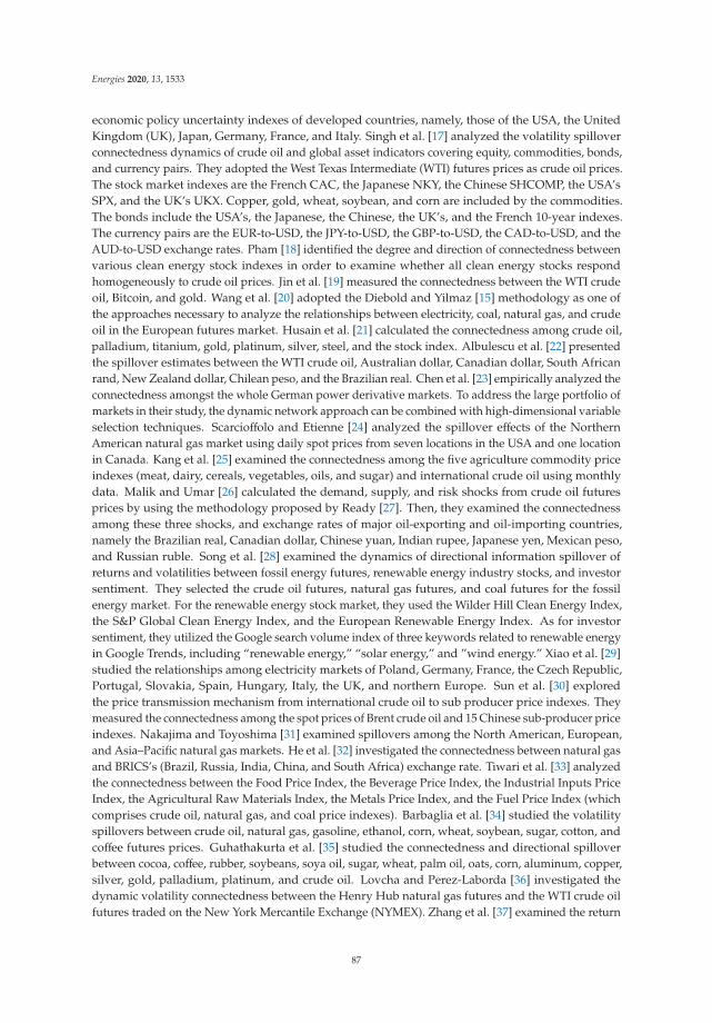
Energies 2020, 13, 1533

economic policy uncertainty indexes of developed countries, namely, those of the USA, the UnitedKingdom (UK), Japan, Germany, France, and Italy. Singh et al. [17] analyzed the volatility spilloverconnectedness dynamics of crude oil and global asset indicators covering equity, commodities, bonds,and currency pairs. They adopted the West Texas Intermediate (WTI) futures prices as crude oil prices.The stock market indexes are the French CAC, the Japanese NKY, the Chinese SHCOMP, the USA’sSPX, and the UK’s UKX. Copper, gold, wheat, soybean, and corn are included by the commodities.The bonds include the USA’s, the Japanese, the Chinese, the UK’s, and the French 10-year indexes.The currency pairs are the EUR-to-USD, the JPY-to-USD, the GBP-to-USD, the CAD-to-USD, and theAUD-to-USD exchange rates. Pham [18] identified the degree and direction of connectedness betweenvarious clean energy stock indexes in order to examine whether all clean energy stocks respondhomogeneously to crude oil prices. Jin et al. [19] measured the connectedness between the WTI crudeoil, Bitcoin, and gold. Wang et al. [20] adopted the Diebold and Yilmaz [15] methodology as one ofthe approaches necessary to analyze the relationships between electricity, coal, natural gas, and crudeoil in the European futures market. Husain et al. [21] calculated the connectedness among crude oil,palladium, titanium, gold, platinum, silver, steel, and the stock index. Albulescu et al. [22] presentedthe spillover estimates between the WTI crude oil, Australian dollar, Canadian dollar, South Africanrand, New Zealand dollar, Chilean peso, and the Brazilian real. Chen et al. [23] empirically analyzed theconnectedness amongst the whole German power derivative markets. To address the large portfolio ofmarkets in their study, the dynamic network approach can be combined with high-dimensional variableselection techniques. Scarcioffolo and Etienne [24] analyzed the spillover effects of the NorthernAmerican natural gas market using daily spot prices from seven locations in the USA and one locationin Canada. Kang et al. [25] examined the connectedness among the five agriculture commodity priceindexes (meat, dairy, cereals, vegetables, oils, and sugar) and international crude oil using monthlydata. Malik and Umar [26] calculated the demand, supply, and risk shocks from crude oil futuresprices by using the methodology proposed by Ready [27]. Then, they examined the connectednessamong these three shocks, and exchange rates of major oil-exporting and oil-importing countries,namely the Brazilian real, Canadian dollar, Chinese yuan, Indian rupee, Japanese yen, Mexican peso,and Russian ruble. Song et al. [28] examined the dynamics of directional information spillover ofreturns and volatilities between fossil energy futures, renewable energy industry stocks, and investorsentiment. They selected the crude oil futures, natural gas futures, and coal futures for the fossilenergy market. For the renewable energy stock market, they used the Wilder Hill Clean Energy Index,the S&P Global Clean Energy Index, and the European Renewable Energy Index. As for investorsentiment, they utilized the Google search volume index of three keywords related to renewable energyin Google Trends, including “renewable energy,” “solar energy,” and ”wind energy.” Xiao et al. [29]studied the relationships among electricity markets of Poland, Germany, France, the Czech Republic,Portugal, Slovakia, Spain, Hungary, Italy, the UK, and northern Europe. Sun et al. [30] exploredthe price transmission mechanism from international crude oil to sub producer price indexes. Theymeasured the connectedness among the spot prices of Brent crude oil and 15 Chinese sub-producer priceindexes. Nakajima and Toyoshima [31] examined spillovers among the North American, European,and Asia–Pacific natural gas markets. He et al. [32] investigated the connectedness between natural gasand BRICS’s (Brazil, Russia, India, China, and South Africa) exchange rate. Tiwari et al. [33] analyzedthe connectedness between the Food Price Index, the Beverage Price Index, the Industrial Inputs PriceIndex, the Agricultural Raw Materials Index, the Metals Price Index, and the Fuel Price Index (whichcomprises crude oil, natural gas, and coal price indexes). Barbaglia et al. [34] studied the volatilityspillovers between crude oil, natural gas, gasoline, ethanol, corn, wheat, soybean, sugar, cotton, andcoffee futures prices. Guhathakurta et al. [35] studied the connectedness and directional spilloverbetween cocoa, coffee, rubber, soybeans, soya oil, sugar, wheat, palm oil, oats, corn, aluminum, copper,silver, gold, palladium, platinum, and crude oil. Lovcha and Perez-Laborda [36] investigated thedynamic volatility connectedness between the Henry Hub natural gas futures and the WTI crude oilfutures traded on the New York Mercantile Exchange (NYMEX). Zhang et al. [37] examined the return

87

Energies 2020, 13, 1533

and volatility spillover among the natural gas, crude oil, and electricity utility stock indexes in NorthAmerica and Europe.

This study applies Diebold and Yilmaz’s [15] technique to the wholesale electricity market andthe natural gas market. We measure the connectedness between power and gas spot returns andfutures returns with different maturities. This study adopts the Henry Hub as the natural gas priceindicator—one of the most representative natural gas price indexes—and the PJM Western Hub Peakas the wholesale electricity price indicator—which is both the most representative of wholesale powerprices and is expected to be the strong link to natural gas prices as marginal cost. This study utilizes eachcommodity’s spot prices and 12 types of futures with one to twelve months maturities. In other words,this study reveals not only the relationship between natural gas prices and wholesale electricity prices,but also the term structure of those prices by measuring the connectedness among these 26 variables.

The calculation results should be able to provide not only novel academic findings, but alsouseful information for practitioners. Especially, the results may be extremely informative for powergeneration companies, which hold huge spots and derivatives for both natural gas as raw material,and power as a product. The fluctuations in the price differences between gas and electricity causesconcern for most practitioners. Their business risks are complicated because they conclude a variety ofprocurement and sales contracts, e.g. sales contracts at a fixed price, procurement contracts at priceslinked to the other price indexes, and long-term contracts of 10 years or more. It is more efficient tocomprehensively evaluate the risks of all contracts that they hold and to hedge their portfolio becauseit is more expensive to hedge each contract individually. Therefore, it is practical and significant toexamine the spillover effects among natural gas and wholesale electricity markets using their futuresprices with various different maturities and their spot prices. The relationships between the naturalgas and electricity markets in various regions have been studied. However, there is no literaturethat analyzes the relationships between natural gas and electricity markets using their futures withmore than 12 different maturities and their spot prices. Although we can analogize the hypothesis ofspillover from the natural gas market to the electricity market from the previous literature, we canexpect to discover some differences caused by different maturities of futures, and some differencesbetween their spot and futures due to their commodity characteristics. The main goal of this study isto clarify these differences.

We can expect twofold results by measuring the spillover indexes between these variables. First, wecan easily understand at a glance the general characteristics of the portfolio. Diebold and Yilmaz’s [15]approach can quantify the degree to which price fluctuations of certain security components of aportfolio have an impact on the portfolio value. Second, we can grasp the market integration amongthese securities with ease. This approach can present the connectedness not only between any twovariables, but also as a whole.

Our contribution to the literature is fourfold. This paper seeks to clarify the relationship andconnectedness between natural gas and wholesale electricity markets’ spot and futures with one totwelve months maturities. First, we explore the spillover effect of each spot market individually.The spillover effect from natural gas spot returns to electricity spot returns is larger than the spillovereffect from gas spot returns to gas futures returns. We argue that the price return of natural gas spothas a greater effect on the price return of wholesale peak power spot, which is directly produced fromgas, than on the price return of natural gas futures by arbitrage trading. On the other hand, we findspillover effects from natural gas futures markets to gas spot markets. We estimate that futures marketshave better natural gas price discovery capabilities than spot markets. Because we do not observe anyevident spillover effects from electricity spot returns to other variables or from all the futures returns toelectricity spot returns, we conclude that power spot prices tend to be dependent on power supply anddemand at that immediate time due to the limitations on arbitrage trading due to the non-storabilityof electricity. Second, we examine the spillover effects of natural gas futures markets. The mutualspillover effects between any gas futures are found. We indicate that the natural gas futures marketis integrated. Third, we examine the relationships between the futures markets of gas and power.

88

Energies 2020, 13, 1533

Our results show spillover effects from natural gas futures returns to power futures returns, whichis consistent with previous studies that support Granger causality from natural gas prices to powerprices. Conversely, we do not see notable spillover effects from electricity futures returns to natural gasfutures returns. Finally, we explore the relationships between power futures markets. We confirm thepresence of spillover effects only between the futures returns with maturity differences of six months.Therefore, we conclude that these effects are not caused by arbitrage trading and that the electricityfutures market is not integrated. The maximum power load, which is the main determinant of theprices, has almost semi-annual seasonality. Therefore, we observe these spillover effects between sixmonths differences maturities just as a single phenomenon.

The remainder of this paper is organized as follows: Section 2 describes the analyzed data,summary statistics, and preliminary basic analyses; Section 3 explains the adopted methodology;Section 4 presents the empirical results; Section 5 provides a summary of the findings and statesthe conclusions.

2. Data and Preliminary Analyses

2.1. Data

We adopt the Henry Hub as the natural gas price indicator in our study. Henry Hub is the nameof a distribution hub of a natural gas pipeline system in the USA. The price of the natural gas deliveredat that hub is the most referenced natural gas price. The Henry Hub futures are listed on the NYMEX.

As our wholesale electricity price indicator, we select the PJM Western Hub Peak. The PJM is oneof the regional electricity transmission organizations that coordinates the generation and distributionof electricity in the USA. We use the peak load price series of the western hub in order to capturethe relationship between natural gas and power. The PJM Western Hub Peak futures are listed onthe NYMEX.

We obtained daily data from January 5, 2009, to December 31, 2018, from Bloomberg. Naturalgas prices and electricity prices are cited in the United States dollars per million British thermal units($/MMBtu) and the United States dollars per megawatt hours ($/MWh), respectively. We obtained eachcommodity’s spot prices and 12 types of futures with one month to twelve months maturities. In otherwords, the relationships between 26 types of economic variables is analyzed.

Figure 1 shows time plots of natural gas prices. We observe that the fluctuations of all the priceseries are almost the same. However, only the natural gas spot price spiked in February 2014 andJanuary 2018.

Figure 1. Time series plots of natural gas prices. (n-months-futures signifies futures with nmonths maturity).

89

Energies 2020, 13, 1533

The reason might be that the natural gas spot market temporally became very tight due to a coldtemperature wave. Natural gas spots cannot be arbitraged easily with their futures. Therefore, sharpfluctuations in its supply and demand cause sharp price fluctuations.

Figure 2 shows the time plots of electricity prices. The relationship between the spot price andeach futures price series is similar to that of the natural gas market. The fluctuations observed in all theprice series are almost similar. However, only the spot price spikes frequently. Because the productionand consumption of electricity occur concurrently, its supply stability requires simultaneous and equalamounts of power supply and demand. In other words, arbitrage between the spot prices and futuresis practically impossible without the use of fuel for power generation. This causes the frequent spikesof the spot prices.

Figure 2. Time series plots of electricity prices. (n-months-futures signifies futures with nmonths maturity).

Table 1 presents the summary statistics of each return series. There are 2452 observations in eachcase. The mean of all series are almost zero. All price series have no trend. In other words, loss fromholding each security is equal to the risk-free interest cost. In the case of both natural gas and electricity,their spot prices have the outstanding largest maximum return and the outstanding smallest minimumreturn, compared to their futures. Therefore, only spot prices might fluctuate differently from thefutures prices. The standard deviations of natural gas spot returns and electricity spot returns indicatethe same. Each sign of skewness has no regularity and is both negative and positive. Most returnseries are right-skewed, whereas the return series of natural gas futures with four, nine, ten, eleven,and twelve months maturity and electricity futures with one month maturity are left-skewed. We findthat all return series are fat-tailed, because their kurtoses have a positive value. Each kurtosis has norelationship with its maturity. The Jarque-Bera statistics calculated from the skewness and kurtosis ofeach series reject the hypothesis that each series is normally distributed.

2.2. Preliminary Analyses

To calculate Diebold and Yilmaz’s [15] index, we need to convert the VAR model to a VMArepresentation with the condition that all variables remain stationary. Accordingly, we apply theaugmented Dickey-Fuller (ADF) unit root test for all series. Table 2 presents the results.

90

Energies 2020, 13, 1533

Table 1. Summary statistics of each return series of natural gas and electricity prices.

Return Series Mean Maximum MinimumStandardDeviation

Skewness KurtosisJarque–Bera

(p-Value)

G0 0.0% 70.1% −43.9% 4.4% 1.5 45.6 186,350 (0)G1 0.0% 26.8% −18.1% 3.1% 0.6 8.3 2983 (0)G2 0.0% 23.4% −22.6% 2.8% 0.3 9.3 4143 (0)G3 0.0% 21.6% −20.2% 2.6% 0.4 9.7 4730 (0)G4 0.0% 18.6% −37.7% 2.5% −1.0 30.9 79,780 (0)G5 0.0% 21.7% −10.1% 2.1% 0.7 9.3 4291 (0)G6 0.0% 19.3% −10.9% 2.0% 0.7 10.1 5398 (0)G7 0.0% 13.7% −11.3% 1.9% 0.4 8.0 2661 (0)G8 0.0% 11.6% −12.8% 1.8% 0.2 7.1 1721 (0)G9 0.0% 13.2% −14.8% 1.7% −0.1 10.0 4954 (0)

G10 0.0% 12.2% −17.7% 1.6% −0.6 13.2 10,680 (0)G11 0.0% 13.0% −17.2% 1.6% −0.7 15.4 15,992 (0)G12 0.0% 11.9% −18.1% 1.5% −0.7 16.9 19,984 (0)

E0 0.0% 203.2% −153.0% 20.2% 0.1 13.8 11,994 (0)E1 0.0% 55.1% −67.0% 5.3% −0.8 42.4 158,546 (0)E2 0.0% 46.7% −45.6% 4.0% 0.5 41.0 147,920 (0)E3 0.0% 37.8% −30.1% 3.4% 1.9 43.2 166,958 (0)E4 0.0% 46.1% −29.5% 3.3% 2.0 57.9 309,913 (0)E5 0.0% 33.7% −30.7% 3.1% 1.1 48.1 208,672 (0)E6 0.0% 40.4% −32.7% 3.2% 1.6 57.7 307,247 (0)E7 0.0% 42.9% −37.5% 3.3% 1.4 63.4 373,262 (0)E8 0.0% 44.7% −29.6% 3.2% 2.2 62.4 362,439 (0)E9 0.0% 40.8% −27.1% 3.1% 1.8 58.1 311,279 (0)

E10 0.0% 39.8% −26.6% 3.1% 1.1 57.0 298,650 (0)E11 0.0% 36.6% −28.9% 3.0% 0.7 56.3 290,411 (0)E12 0.0% 33.2% −32.1% 3.1% 0.6 52.2 247,347 (0)

Note: G0 signifies natural gas spot. Gn signifies natural gas futures with n months maturity. E0 signifies electricityspot. En signifies electricity futures with n months maturity.

Table 2. Unit root tests.

Return SeriesAugmented Dickey-Fuller–t Value (p-Value)

Exogenous: Constant Exogenous: Constant, Trend

G0 −16.34 (0.000) −16.34 (0.000)G1 −53.70 (0.000) −53.69 (0.000)G2 −54.08 (0.000) −54.08 (0.000)G3 −53.27 (0.000) −53.27 (0.000)G4 −53.59 (0.000) −53.59 (0.000)G5 −33.63 (0.000) −33.62 (0.000)G6 −29.50 (0.000) −29.50 (0.000)G7 −52.53 (0.000) −52.52 (0.000)G8 −52.42 (0.000) −52.41 (0.000)G9 −52.59 (0.000) −52.59 (0.000)

G10 −52.50 (0.000) −52.50 (0.000)G11 −53.17 (0.000) −53.18 (0.000)G12 −30.07 (0.000) −30.09 (0.000)

E0 −22.95 (0.000) −22.95 (0.000)E1 −48.01 (0.000) −48.00 (0.000)E2 −21.03 (0.000) −21.03 (0.000)E3 −48.29 (0.000) −48.28 (0.000)E4 −49.58 (0.000) −49.57 (0.000)E5 −49.46 (0.000) −49.45 (0.000)E6 −50.06 (0.000) −50.05 (0.000)E7 −50.44 (0.000) −50.43 (0.000)E8 −49.54 (0.000) −49.53 (0.000)E9 −48.79 (0.000) −48.78 (0.000)

E10 −48.75 (0.000) −48.74 (0.000)E11 −49.92 (0.000) −49.91 (0.000)E12 −50.38 (0.000) −50.38 (0.000)

Note: G0 signifies natural gas spot. Gn signifies natural gas futures with n months maturity. E0 signifies electricityspot. En signifies electricity futures with n months maturity.

The ADF test rejects the null hypothesis that all variables are non-stationary. Therefore, we canconfirm the availability of the VMA representation.

3. Methodology

We calculate the spillover index proposed by Diebold and Yilmaz [15] in order to capture therelationship between economic variables. This approach can reveal not only pairwise connectednessbetween any two variables, but also total connectedness between all variables.

91

Energies 2020, 13, 1533

We consider the following covariance stationary twenty-six-variable VAR (p):

rt =

p∑k=1

Φkrt−k + εt, (1)

where rt is the twenty-six-dimensional vector of return, which must be a stationary series; Φk are the26× 26 coefficient matrices; p is the lag length determined by minimizing the Schwarz informationcriterion; and εt is an independently and identically distributed sequence of twenty-six-dimensionalrandom vectors with zero mean and covariance matrix E

(εtε′t

)= Σ.

We can represent the above covariance stationary twenty-six-variable VAR model in the followingVMA:

rt =∞∑

k=0

Akεt−k (2)

where Ak =∑p

k=1 ΦkAt−k, A0 being a 26× 26 identity matrix with Ak = 0 for k < 0.The spillover effect from the lth to the kth market up to H-step-ahead is defined as the following

equation by using the H-step-ahead forecast error variance decompositions:

θkl =σ−1

ll∑H−1

h=0

(e′kAhΣel

)2∑H−1h=0 e′kAhΣA′

hek(3)

where σll is the standard deviation of the error term for the lth equation and ek is the selection vector,with one as the kth element and zeros otherwise.

Each entry of the variance decomposition matrix is normalized by the row sum, that is, 26, as thepairwise connectedness:

θkl =θkl∑26

l=1 θkl=θkl26

(4)

The sum of pairwise connectedness is defined as total connectedness:

S =

∑26k=1

∑26l=1,k�l θkl

26(5)

The numerator is the sum of the spillover effects. However, each spillover effect on itself isdeducted. In other words, the total connectedness means the sum of the relative proportion of theportfolio’s response to a shock.

Moreover, the directional spillover effects received by the kth market from all other markets ismeasured as:

Sk· =∑26

k=1,k�l θkl

26(6)

Similarly, the directional spillover effects transmitted by the kth market to all other markets ismeasured as:

S·k =∑26

k=1,k�l θlk

26(7)

4. Empirical Results

Table 3 presents the spillover analysis results. This table shows total connectedness, all 676 (= 26× 26) pairwise connectedness, all 26 directional spillover effects received from all other variables, andall 26 directional spillover effects transmitted to all other variables. The cells in this table are paintedgradually from white to dark green, with white representing 0% and dark green representing 10%or more.

92

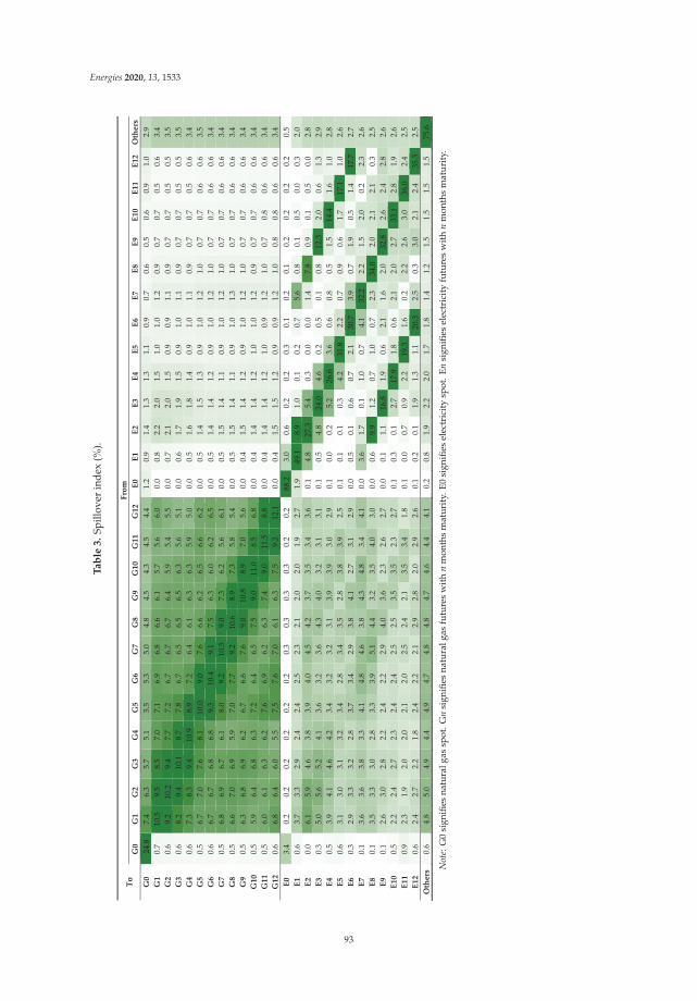
Energies 2020, 13, 1533

Ta

ble

3.

Spill

over

inde

x(%

).

To

From

G

0 G

1 G

2 G

3 G

4 G

5 G

6 G

7 G

8 G

9 G

10

G11

G

12

E0

E1

E2

E3

E4

E5

E6

E7

E8

E9

E10

E11

E12

Oth

ers

G0

24.8

7.

4 6.

3 5.

7 5.

1 5.

5 5.

3 5.

0 4.

8 4.

5 4.

3 4.

5 4.

4 1.

2 0.

9 1.

4 1.

3 1.

3 1.

1 0.

9 0.

7 0.

6 0.

5 0.

6 0.

9 1.

0 2.

9 G

1 0.

7 10

.5

9.5

8.5

7.0

7.1

6.9

6.8

6.6

6.1

5.7

5.6

6.0

0.0

0.8

2.2

2.0

1.5

1.0

1.0

1.2

0.9

0.7

0.7

0.5

0.6

3.4

G2

0.6

9.2

10.2

9.

4 7.

7 7.

2 6.

7 6.

7 6.

7 6.

4 5.

9 5.

4 5.

5 0.

0 0.

7 2.

1 2.

0 1.

5 0.

9 0.

9 1.

1 0.

9 0.

7 0.

7 0.

5 0.

5 3.

5 G

3 0.

6 8.

2 9.

4 10

.1

8.7

7.8

6.7

6.5

6.5

6.5

6.3

5.6

5.1

0.0

0.6

1.7

1.9

1.5

0.9

1.0

1.1

0.9

0.7

0.7

0.5

0.5

3.5

G4

0.6

7.3

8.3

9.4

10.9

8.

9 7.

2 6.

4 6.

1 6.

3 6.

3 5.

9 5.

0 0.

0 0.

5 1.

6 1.

8 1.

4 0.

9 1.

0 1.

1 0.

9 0.

7 0.

7 0.

5 0.

6 3.

4 G

5 0.

5 6.

7 7.

0 7.

6 8.

1 10

.0

9.0

7.6

6.6

6.2

6.5

6.6

6.2

0.0

0.5

1.4

1.5

1.3

0.9

1.0

1.2

1.0

0.7

0.7

0.6

0.6

3.5

G6

0.6

6.7

6.7

6.8

6.8

9.3

10.4

9.

1 7.

5 6.

3 6.

0 6.

2 6.

5 0.

0 0.

5 1.

4 1.

4 1.

2 0.

9 1.

0 1.

2 1.

0 0.

7 0.

7 0.

6 0.

6 3.

4 G

7 0.

5 6.

8 6.

9 6.

7 6.

1 8.

0 9.

2 10

.5

9.0

7.3

6.2

5.6

6.1

0.0

0.5

1.5

1.4

1.1

0.9

1.0

1.2

1.0

0.7

0.7

0.6

0.6

3.4

G8

0.5

6.6

7.0

6.9

5.9

7.0

7.7

9.2

10.6

8.

9 7.

3 5.

8 5.

4 0.

0 0.

5 1.

5 1.

4 1.

1 0.

9 1.

0 1.

3 1.

0 0.

7 0.

7 0.

6 0.

6 3.

4 G

9 0.

5 6.

3 6.

8 6.

9 6.

2 6.

7 6.

6 7.

6 9.

0 10

.8

8.9

7.0

5.6

0.0

0.4

1.5

1.4

1.2

0.9

1.0

1.2

1.0

0.7

0.7

0.6

0.6

3.4

G10

0.

5 5.

9 6.

4 6.

8 6.

3 7.

2 6.

4 6.

5 7.

5 9.

0 11

.0

8.5

6.8

0.0

0.4

1.4

1.4

1.2

1.0

1.0

1.2

0.9

0.7

0.7

0.6

0.6

3.4

G11

0.

5 6.

0 6.

1 6.

3 6.

2 7.

6 6.

9 6.

2 6.

3 7.

4 9.

0 11

.5

8.8

0.0

0.4

1.4

1.4

1.2

1.0

0.9

1.2

1.0

0.7

0.8

0.6

0.6

3.4

G12

0.

6 6.

8 6.

4 6.

0 5.

5 7.

5 7.

6 7.

0 6.

1 6.

3 7.

5 9.

2 12

.1

0.0

0.4

1.5

1.5

1.2

0.9

0.9

1.2

1.0

0.8

0.8

0.6

0.6

3.4

E0

3.4

0.2

0.2

0.2

0.2

0.2

0.2

0.3

0.3

0.3

0.3

0.2

0.2

88.2

3.

0 0.

6 0.

2 0.

2 0.

3 0.

1 0.

2 0.

1 0.

2 0.

2 0.

2 0.

2 0.

5 E1

0.

6 3.

7 3.

3 2.

9 2.

4 2.

4 2.

5 2.

3 2.

1 2.

0 2.

0 1.

9 2.

7 1.

9 49

.1

8.9

1.0

0.1

0.2

0.7

5.6

0.8

0.1

0.5

0.0

0.3

2.0

E2

0.0

6.1

5.9

4.6

3.8

3.9

4.0

4.5

4.2

3.7

3.5

3.4

3.6

0.1

4.8

27.3

5.

4 0.

3 0.

0 0.

0 1.

4 7.

8 0.

9 0.

1 0.

5 0.

0 2.

8 E3

0.

3 5.

0 5.

6 5.

2 4.

1 3.

6 3.

2 3.

6 4.

3 4.

0 3.

2 3.

1 3.

1 0.

1 0.

5 4.

8 24

.0

4.6

0.2

0.5

0.1

0.8

12.3

2.

0 0.

6 1.

3 2.

9 E4

0.

5 3.

9 4.

1 4.

6 4.

2 3.

4 3.

2 3.

2 3.

1 3.

9 3.

9 3.

0 2.

9 0.

1 0.

0 0.

2 5.

2 26

.6

3.6

0.6

0.8

0.5

1.5

14.4

1.

6 1.

0 2.

8 E5

0.

6 3.

1 3.

0 3.

1 3.

2 3.

4 2.

8 3.

4 3.

5 2.

8 3.

8 3.

9 2.

5 0.

1 0.

1 0.

1 0.

3 4.

2 31

.8

2.2

0.7

0.9

0.6

1.7

17.1

1.

0 2.

6 E6

0.

3 2.

9 3.

3 3.

2 2.

8 3.

7 3.

4 2.

9 3.

8 4.

1 2.

7 3.

1 2.

9 0.

0 0.

5 0.

1 0.

6 0.

7 2.

1 30

.7

3.9

0.7

1.9

0.5

1.4

17.7

2.

7 E7

0.

1 3.

6 3.

6 3.

8 3.

3 4.

1 4.

8 4.

6 3.

8 4.

3 4.

8 3.

4 4.

1 0.

0 3.

6 1.

7 0.

1 1.

0 0.

7 4.

1 32

.2

2.2

1.5

2.0

0.2

2.3

2.6

E8

0.1

3.5

3.3

3.0

2.8

3.3

3.9

5.1

4.4

3.2

3.5

4.0

3.0

0.0

0.6

9.9

1.2

0.7

1.0

0.7

2.3

34.0

2.

0 2.

1 2.

1 0.

3 2.

5 E9

0.

1 2.

6 3.

0 2.

8 2.

2 2.

4 2.

2 2.

9 4.

0 3.

6 2.

3 2.

6 2.

7 0.

0 0.

1 1.

1 16

.8

1.9

0.6

2.1

1.6

2.0

32.8

2.

6 2.

4 2.

8 2.

6 E1

0 0.

5 2.

2 2.

4 2.

7 2.

3 2.

4 2.

4 2.

5 2.

5 3.

5 3.

5 2.

3 2.

7 0.

1 0.

3 0.

1 2.

7 17

.9

1.8

0.6

2.1

2.0

2.7

33.1

2.

8 1.

9 2.

6 E1

1 0.

9 2.

3 1.

9 2.

0 2.

0 2.

1 2.

0 2.

5 2.

4 2.

1 3.

5 3.

4 1.

8 0.

1 0.

0 0.

7 0.

9 2.

2 19

.3

1.6

0.2

2.2

2.6

3.0

36.0

2.

4 2.

5 E1

2 0.

6 2.

4 2.

7 2.

2 1.

8 2.

4 2.

2 2.

1 2.

9 2.

8 2.

0 2.

9 2.

6 0.

1 0.

2 0.

1 1.

9 1.

3 1.

1 20

.3

2.5

0.3

3.0

2.1

2.4

35.3

2.

5 O

ther

s 0.

6 4.

8 5.

0 4.

9 4.

4 4.

9 4.

7 4.

8 4.

8 4.

7 4.

6 4.

4 4.

1 0.

2 0.

8 1.

9 2.

2 2.

0 1.

7 1.

8 1.

4 1.

2 1.

5 1.

5 1.

5 1.

5 75

.6

Not

e:G

0si

gnifi

esna

tura

lgas

spot

.Gn

sign

ifies

natu

ralg

asfu

ture

sw

ith

nm

onth

sm

atur

ity.

E0si

gnifi

esel

ectr

icit

ysp

ot.E

nsi

gnifi

esel

ectr

icit

yfu

ture

sw

ith

nm

onth

sm

atur

ity.

93

Energies 2020, 13, 1533

4.1. Between Spot and Others

We cannot find spillover effects from natural gas spot returns to the other variables except forelectricity spot returns (see column G0 of Table 3). The pairwise connectedness from gas spot returnsto power spot returns is 3.4% (see row E0 and column G0 in Table 3). We estimate that it is practicallydifficult to arbitrage gas and electricity futures markets by renting or lending the cash position ofnatural gas. Due to the quantitative and cost constraints for storing natural gas, natural gas spotprices are more likely to be transmitted to natural gas-fueled peak electricity spot prices than naturalgas futures.

The spillover effects from all the gas futures returns to gas spot returns are observed (see row G0and columns G1 to G12 in Table 3). Although the spot market is susceptible to irregular trading andmomentary fluctuations in its supply and demand, the futures markets have enough time to reflect theinformation related to its price formation, as long as its liquidity is high. Therefore, futures marketshave better natural gas price discovery capabilities than spot markets. The pairwise spillover indexfrom electricity futures returns with each maturity to natural gas spot returns is small.

No spillover effects from electricity spot returns to the other variables (see row E0 in Table 3) andfrom all the futures returns to electricity spot returns occur (see row E0 in Table 3). Electricity spotprices are dependent on the power generation costs and the power market conditions at that timebecause the non-storability of electricity limits arbitrage trading.

Nakajima [38] and Moutinho et al. [39] examined the relationship between natural gas andwholesale electricity spot prices in Japan and Spain, respectively. Their results reject the hypothesisof the Granger causality between gas and power prices. We cannot argue that the pairwiseconnectedness indicators between gas and electricity spot returns are consistent with Nakajima [38]and Moutinho et al. [39]. This is assumed to be due to differences between Granger causality andspillover effects and/or regional differences.

4.2. Between Natural Gas Futures

The pairwise spillover indexes between any natural gas futures returns are over 5%, while thespillover effect from each natural gas futures return to itself is about 11% (see rows G1 to G12 andcolumns G1 to G12 in Table 3). In other words, the natural gas futures market is mostly integrated.Especially, the gas futures markets with a month maturity and with two months maturity are perfectlyintegrated, because the spillover indexes from these futures returns to themselves are 10.5% (seerow G1 and column G1 in Table 3) and 10.2% (see row G2 and column G2 in Table 3), while theindexes from themselves to each other are 9.2% (see row G1 and column G2 in Table 3) and 9.5%(see row G2 and column G1 in Table 3). Furthermore, the spillover effect indexes between futuresreturns with close maturity differences tend to be greater than those between futures returns with longmaturity differences.

4.3. Between Natural Gas Futures and Electricity Futures

We can observe the spillover effects from natural gas futures returns with each maturity towholesale electricity futures returns with each maturity (see rows E1 to E12 and columns G1 to G12 inTable 3). These calculated results are consistent with previous studies that conclude a Granger causalityfrom natural gas prices to power prices (see Emery and Liu [3] which is one of the most representativeprevious studies which examines the relationship between natural gas and electricity futures prices).The pairwise spillover indexes from the natural gas futures returns to the electricity futures returnswith around the same maturity are larger. The natural gas futures prices with certain maturity affectnot only the natural gas futures prices with other maturities, but also the peak power futures prices.The pairwise spillover index from the natural gas futures returns with a one-month period maturity tothe wholesale electricity futures returns with a two-month period maturity is 6.1% (see row E2 andcolumn G1 in Table 3).

94

Energies 2020, 13, 1533

Conversely, spillover effects from electricity futures to natural gas futures are hardly found (seerows G1 to G12 and columns E1 to E12 in Table 3). The maximum is the pairwise index from theelectricity futures returns with a two-month maturity period to natural gas futures returns with aone-month maturity period, which is only 2.2% (see row G1 and column E2 in Table 3). The relativelyaccurate forecast of electricity demand after two months might affect not only the peak power futuresprices but also the fuel futures.

4.4. Between Electricity Futures

We cannot confirm spillover effects between wholesale electricity futures returns, except for thespillover effects between futures returns with maturity differences of six months (see rows E1 to E12and columns E1 to E12 in Table 3). We should interpret these results by understanding the relationshipbetween the futures price formation and the features of this commodity differently from traditionalfinancial securities.

Futures prices are primarily the expected prices at maturity. However, we should considerarbitrage trading in the spot market. By considering the cost of carrying over the spot position tothe maturity of the futures including the opportunity costs and the risk of holding the spot position,we can obtain a non-arbitrage conditional equation for the spot prices and the futures prices. Usingthis equation, each spot price gives us a unique futures price. However, electricity is a good that isconsumed at the same time that it is produced meaning we cannot store electric energy easily. In otherwords, arbitrage between the electricity spot market and futures markets is practically impossible.Spread trading between futures markets with different maturities is impossible as well, although wecannot deny electricity arbitrage trading through the fuel markets.

On the other hand, the main determinant of electricity prices is the load at that time. Therefore,peak power prices are affected by maximum power loads, which have almost semi-annual seasonality.Table 4 presents the correlation coefficients between the monthly average values of the daily maximumloads. The correlation coefficient between six-month differences is close to one. Moreover, wecalculate the correlation coefficients between electricity futures of different maturity to understand thesimultaneous relationship as a phenomenon. In Table 5, which shows those coefficients, we observethat the correlation coefficients between six-month differences are relatively large. The cells in this tableare painted gradually from white to green, with white representing 0 and dark green representing 1.

Table 4. Correlation coefficients between maximum loads.

Months Difference 1 2 3 4 5 6

Correlation coefficients 0.32 −0.35 −0.88 −0.37 0.38 0.80

Table 5. Correlation coefficients between electricity futures.

Return Series E1 E2 E3 E4 E5 E6 E7 E8 E9 E10 E11 E12 E1 1.00

E2 0.43 1.00

E3 0.05 0.42 1.00

E4 0.10 0.05 0.41 1.00

E5 0.01 0.22 0.21 0.39 1.00

E6 0.15 0.06 0.33 0.24 0.32 1.00

E7 0.40 0.29 0.15 0.37 0.25 0.37 1.00

E8 0.17 0.63 0.24 0.24 0.39 0.24 0.33 1.00

E9 0.10 0.22 0.77 0.25 0.25 0.42 0.27 0.30 1.00

E10 0.20 0.14 0.31 0.79 0.29 0.23 0.43 0.31 0.32 1.00

E11 0.10 0.30 0.20 0.32 0.79 0.24 0.23 0.44 0.30 0.36 1.00

E12 0.10 0.11 0.39 0.23 0.29 0.81 0.28 0.24 0.45 0.28 0.32 1.00

Note: En signifies electricity futures with n months maturity.

95

Energies 2020, 13, 1533

Therefore, we should interpret these spillover effects between six-month maturity differences justas a seasonal phenomenon. The electricity futures market cannot be considered integrated.

5. Conclusions

We have adopted Diebold and Yilmaz’s [15] approach to examine the spillover effects amongnatural gas and wholesale electricity markets using their futures with different maturities and theirspot prices. We used daily data from January 5, 2009, to December 31, 2018, and employed the HenryHub and the PJM Western Hub Peak as the natural gas price indicator and the wholesale electricityprice indicator, respectively. We obtained each commodity’s spot prices and 12 types of futures withone to twelve months maturities. In other words, we analyzed the relationships between 26 types ofeconomic variables.

The main results of our analyses are fourfold. First, we find that there are mutual spillovereffects amongst natural gas futures returns showing that the natural gas futures market is integrated.The possession of futures with many different maturities has a low diversification effect on a portfolio,although it is effective for directly hedging the spot trading at the applicable maturity. It is reasonableto hold the futures with two-, three-, and four-month period maturities, because these futures largelyaffect the other variables (see the row Others and columns G2 to G4 in Table 3) and all futures areequally affected by the other variables (see rows G1 to G12 and the column Others in Table 3).

Second, our results show that there are spillover effects from natural gas futures returns to naturalgas spot returns, although no spillover effects from natural gas spot returns to natural gas futuresreturns are evident. From this, we conclude that futures markets have better natural gas price discoverycapabilities than spot markets. The natural gas futures markets indicate the prices expected from thelong-term economic environment surrounding natural gas. The natural gas spot prices often deviatefrom their fundamentals because the storage cost is extremely expensive, and the spot prices dependon their fluctuations in supply and demand at that immediate time. Therefore, the futures prices mustbe utilized when formulating government policies and/or business plans.

Third, we observe spillover effects from natural gas spot returns to electricity spot returns aswell as spillover effects from natural gas futures returns to electricity futures returns. The spillovereffects from natural gas spot returns to electricity spot returns are larger than the spillover effect fromnatural gas spot returns to natural gas futures returns. We thus argue that the marginal cost of powergeneration (natural gas prices) is passed through to electricity prices. The natural gas futures marketsare extremely useful in order to control the risks from the electricity markets.

Finally, our results do not show any spillover effects amongst electricity futures returns, exceptfor some combinations, or any spillover effects from electricity futures returns to natural gas futuresreturns. We confirm the presence of spillover effects between futures with a maturity difference ofsix months only, concluding these as merely a singular phenomenon. This means it is not caused byarbitrage trading. The maximum power load, which is the main determinant of the prices, has analmost semi-annual seasonality. Thus, we conclude that the electricity futures market is not integrated.We might expect diversification effects by the possession of the futures with many different maturities.However, it is necessary to pay attention to the seasonality in the selection.

Author Contributions: Conceptualization, T.N.; Data curation, T.N.; Formal analysis, T.N.; Validation, Y.T.;Visualization, T.N.; Writing—original draft, T.N.; Writing—review & editing, T.N. All authors have read andagreed to the published version of the manuscript.


Acknowledgments: The authors would like to thank the anonymous reviewers, whose valuable comments helpedimprove an earlier version of this paper.

Conflicts of Interest: The authors declare no conflicts of interest.

96

Energies 2020, 13, 1533

References

1. BP p.l.c., 1 St James’s Square, London SW1Y 4PD, UK. BP’s Statistical Review of World Energy 2019, 68thed. Available online: https://www.bp.com/content/dam/bp/business-sites/en/global/corporate/pdfs/energy-economics/statistical-review/bp-stats-review-2019-full-report.pdf (accessed on 4 February 2020).

2. Serletis, A.; Herbert, J. The message in North American energy prices. Energy Econ. 1999, 21, 471–483.[CrossRef]

3. Emery, G.W.; Liu, W.Q. An analysis of the relationship between electricity and natural-gas futures prices.J. Futures Mark. 2002, 22, 95–122. [CrossRef]

4. Woo, C.; Olson, A.; Horowitz, I.; Luk, S. Bi-directional causality in California’s electricity and natural-gasmarkets. Energy Policy 2006, 34, 2060–2070. [CrossRef]

5. Serletis, A.; Shahmoradi, A. Measuring and testing natural gas and electricity markets volatility: Evidencefrom Alberta’s deregulated markets. Stud. Nonlinear Dyn. Econ. 2006, 10, 10. [CrossRef]

6. Brown, S.P.A.; Yücel, M.K. Deliverability and regional pricing in U.S. natural gas markets. Energy Econ. 2008,30, 2441–2453. [CrossRef]

7. Mjelde, J.W.; Bessler, D.A. Market integration among electricity markets and their major fuel source markets.Energy Econ. 2009, 31, 482–491. [CrossRef]

8. Mohammadi, H. Electricity prices and fuel costs: Long-run relations and short-run dynamics. Energy Econ.2009, 31, 503–509. [CrossRef]

9. Nakajima, T.; Hamori, S. Testing causal relationships between wholesale electricity prices and primaryenergy prices. Energy Policy 2013, 62, 869–877. [CrossRef]

10. Toda, H.Y.; Yamamoto, T. Statistical inference in vector autoregressions with possibly integrated processes.J. Econ. 1995, 66, 225–250. [CrossRef]

11. Cheung, Y.W.; Ng, L.K. A causality-in-variance test and its application to financial market prices. J. Econ.1996, 72, 33–48. [CrossRef]

12. Efimova, O.; Serletis, A. Energy markets volatility modelling using GARCH. Energy Econ. 2014, 43, 264–273.[CrossRef]

13. Alexopoulos, T.A. The growing importance of natural gas as a predictor for retail electricity prices in USA.Energy 2017, 137, 219–233. [CrossRef]

14. Nakajima, T. Expectations for statistical arbitrage in energy futures markets. J. Risk Financ. Manag. 2019, 12,14. [CrossRef]

15. Diebold, F.X.; Yilmaz, K. Better to give than to receive: Predictive directional measurement of volatilityspillovers. Int. J. Forecast. 2012, 28, 57–66. [CrossRef]

16. Yang, L. Connectedness of economic policy uncertainty and oil price shocks in a time domain perspective.Energy Econ. 2019, 80, 219–233. [CrossRef]

17. Singh, V.K.; Kumar, P.; Nishant, S. Feedback spillover dynamics of crude oil and global assets indicators:A system-wide network perspective. Energy Econ. 2019, 80, 321–335. [CrossRef]

18. Pham, L. Do all clean energy stocks respond homogeneously to oil price? Energy Econ. 2019, 81, 355–379.[CrossRef]

19. Jin, J.; Yu, J.; Hu, Y.; Shang, Y. Which one is more informative in determining price movements of hedgingassets? Evidence from Bitcoin, gold and crude oil markets. Phys. A 2019, 527, 121121. [CrossRef]

20. Wang, B.; Wei, Y.; Xing, Y.; Ding, W. Multifractal detrended cross-correlation analysis and frequency dynamicsof connectedness for energy futures markets. Phys. A 2019, 527, 121194. [CrossRef]

21. Husain, S.; Tiwari, A.K.; Sohag, K.; Shahbaz, M. Connectedness among crude oil prices, stock index andmetal prices: An application of network approach in the USA. Resour. Policy 2019, 62, 57–65. [CrossRef]

22. Albulescu, C.T.; Demirer, R.; Raheem, I.D.; Tiwari, A.K. Does the U.S. economic policy uncertainty connectfinancial markets? Evidence from oil and commodity currencies. Energy Econ. 2019, 83, 375–388. [CrossRef]

23. Chen, S.; Härdle, W.K.; Cabrera, B.L. Regularization approach for network modeling of German powerderivative market. Energy Econ. 2019, 83, 180–196. [CrossRef]

24. Scarcioffolo, A.R.; Etienne, X.L. How connected are the U.S. regional natural gas markets in thepost-deregulation era? Evidence from time-varying connectedness analysis. J. Commod. Mark. 2019,15, 100076. [CrossRef]

97

Energies 2020, 13, 1533

25. Kang, S.H.; Tiwari, A.K.; Albulescu, C.T.; Yoon, S.M. Exploring the time-frequency connectedness andnetwork among crude oil and agriculture commodities V1. Energy Econ. 2019, 84, 104543. [CrossRef]

26. Malik, F.; Umar, Z. Dynamic connectedness of oil price shocks and exchange rates. Energy Econ. 2019, 84,104501. [CrossRef]

27. Ready, R.C. Oil Prices and the Stock Market. Rev. Financ. 2018, 22, 155–176. [CrossRef]28. Song, Y.; Ji, Q.; Du, Y.; Geng, J. The dynamic dependence of fossil energy, investor sentiment and renewable

energy stock markets. Energy Econ. 2019, 84, 104564. [CrossRef]29. Xiao, B.; Yang, Y.; Peng, X.; Fang, L. Measuring the connectedness of European electricity markets using the

network topology of variance decompositions. Phys. A 2019, 535, 122279. [CrossRef]30. Sun, Q.; An, H.; Gao, X.; Guo, S.; Wang, Z.; Liu, S.; Wen, S. Effects of crude oil shocks on the PPI system

based on variance decomposition network analysis. Energy 2019, 189, 116378. [CrossRef]31. Nakajima, T.; Toyoshima, Y. Measurement of connectedness and frequency dynamics in global natural gas

markets. Energies 2019, 12, 3927. [CrossRef]32. He, Y.; Nakajima, T.; Hamori, S. Connectedness between natural gas price and BRICS exchange rates:

Evidence from time and frequency domains. Energies 2019, 12, 3970. [CrossRef]33. Tiwari, A.K.; Nasreen, S.; Shahbaz, M.; Hammoudeh, S. Time-frequency causality and connectedness

between international prices of energy, food, industry, agriculture and metals. Energy Econ. 2020, 85, 104529.[CrossRef]

34. Barbaglia, L.; Croux, C.; Wilms, I. Volatility spillovers in commodity markets: A large t-vector autoregressiveapproach. Energy Econ. 2020, 85, 104555. [CrossRef]

35. Guhathakurta, K.; Dash, S.R.; Maitra, D. Period specific volatility spillover based connectedness between oiland other commodity prices and their portfolio implications. Energy Econ. 2020, 85, 104566. [CrossRef]

36. Lovcha, Y.; Perez-Laborda, A. Dynamic frequency connectedness between oil and natural gas volatilities.Econ. Model. 2020, 84, 181–189. [CrossRef]

37. Zhang, W.; He, X.; Nakajima, T.; Hamori, S. How does the spillover among natural gas, crude oil, andelectricity utility stocks change over time? Evidence from North America and Europe. Energies 2020, 13, 727.[CrossRef]

38. Nakajima, T. Inefficient and opaque price formation in the Japan Electric Power Exchange. Energy Policy2013, 55, 329–334. [CrossRef]

39. Moutinho, V.; Vieira, J.; Moreira, A.C. The crucial relationship among energy commodity prices: Evidencefrom the Spanish electricity market. Energy Policy 2011, 39, 5898–5908. [CrossRef]


98

energies

Article

Can One Reinforce Investments in Renewable EnergyStock Indices with the ESG Index?

Guizhou Liu and Shigeyuki Hamori *

Graduate School of Economics, Kobe University, 2-1, Rokkodai, Nada-Ku, Kobe 657-8501, Japan;[email protected]* Correspondence: [email protected]

Received: 8 January 2020; Accepted: 27 February 2020; Published: 4 March 2020

Abstract: Studies on the environmental, social, and governance (ESG) index have become increasinglyimportant since the ESG index offers attractive characteristics, such as environmental friendliness.Scholars and institutional investors are evaluating if investment in the ESG index can positivelychange current portfolios. It is crucial that institutional investors seek related assets to diversify theirinvestments when such investors create funds in the renewable energy sector, which is highly relatedto environmental issues. The ESG index has proven to be a good investment choice, but we are notaware of its performance when combined with renewable energy securities. To uncover this nature,we investigate the dependence structure of the ESG index and four renewable energy indices withconstant and time-varying copula models and evaluate the potential performance of using differentratios of the ESG index in the portfolio. Criteria such as risk-adjusted return, standard deviation,and conditional value-at-risk (CVaR) show that the ESG index can provide satisfactory results inlowering the potential CVaR and maintaining a high return. A goodness-of-fit test is then used toensure the results obtained from the copula models.

Keywords: ESG; renewable energy; copula; value-at-risk

1. Introduction

In this paper, we seek to illustrate the relationship between the environmental, social,and governance (ESG) index and the renewable energy index. Meanwhile, we want to revealthe potential in combining investments into a portfolio and constructing an index combination thatperforms better than pre-existing ones. Many institutional investors are focusing on renewable energyinvestment; these investment portfolios use the renewable energy index as a benchmark, comparedto other investment methods, thereby making them much more valuable with a lower exposure topotentially large financial risk. For example, “iShares trust global clean energy ETF” regards “the S&Pglobal clean energy index” as the benchmark, investing 90% of its assets on stocks from the index andothers on futures, options, and other contracts. It is also reasonable for large institutional investorsto choose stocks or contracts that are full of liquidity and helpful in hedging potential financial risk.For institutional investors, finding a way to reinforce the return yield of their investments in certainfields is the first priority. To reinforce these investments, there should be other types of stocks or bondscontained in the portfolio that are also related to the topic of green energy. After the reinforcement ofan investment, the ideal result will be a higher level of returns with a certain risk and a lower level ofvalue at that risk (i.e., the expected shortfall). Of course, diversification will also decrease the potentialvariation of the investment value. For funds related to the renewable energy index, the ESG index maybe a good choice. The ESG index (here, we mainly use the S&P 500 ESG Index (USD) as our researchtarget) is familiar to numerous global investors that are interested in selecting securities with a highstandard of sustainability criteria. The ESG refers to environmental, social, and governance factors;


Energies 2020, 13, 1179

listed companies with these qualifications will normally outperform other companies by providinghigher performance in stock prices and bond returns. The ESG index will normally include similaroverall sector weights. We want to further investigate if large institutional investors should considerincluding the ESG index in their investments in the renewable energy sector. There are many selectionsof ETFs, so we use the index as a substitute for detailed portfolios.

The companies listed in the ESG index are normally attractive investments [1] investigated “greenbonds” and companies issuing appealing bonds. Companies have significant incentive to financethemselves by issuing “green bonds”. Through these bonds, companies can obtain more attention fromthe capital market by increasing their ESG score, thereby boosting their stock prices if they are listed.Once the firms are labeled as ‘green’ and have enough media exposure, they can raise the marketdemand for their shares. Those companies obtaining greater rewards in environmental managementcan positively influence their stock price returns [2]. In summary, at the level of company revenueand stock prices, achieving a higher ESG score or being elected into the ESG index is beneficial for thecompanies by getting them greater attention and more public media exposure.

For institutional investors, such as fund managers holding securities, futures, and forwardcontracts of environmental interest (in this paper, we mainly focus on the renewable energy index), ESGissues can also be beneficial for portfolio management. There is an association between safeguardingliquidity and hedging [3]; in this paper, we want to prove that the ESG index can be safeguardingtools for renewable energy indices. In previous literatures, the association is proved to exist betweenstrategic cash and lines of credit [4], indicating that the leverage can yield future business opportunitiesin good times, while the current nonoperational cash can provide guards against cash flow variation.It is also a decent choice for institutional investors to develop the hedging strategies applying futuresand forward contracts [5], which are traded actively in fields of renewable energy sector.

The connection between renewable energy and institutional investors are closer than before asthe institutional investors keep providing liquidity for the ESG index and renewable energy sector.In many OECD countries, the current situation are low interest rate environment and weak economicgrowth, in which institutional investors are seeking assets such as renewable energy that providesteady return that have low correlation with other choices of assets [6]. The engagement in the ESGindex can help increase potential accounting performance [7]; on the other hand, this index maybe successful in reducing possible financial risk, as proven and measured by Hoepner et al. [8], inlower partial moments and value at risk. Meanwhile, investments on the ESG index will graduallymotivate the companies in enhancing their business in a more friendly way and help the framing ofregulations [9].

To study the combined performance of using multiple indices (corresponding to ETF), we needto illustrate the dependence structure of the ingredients and then examine the detailed performanceof possible portfolios. In the field of energy-related securities investment, scholars use Grangercasualty [10], the wavelet-based test [11], and copula models [12] to study the co-movements andvolatility spillovers among energy stock prices or indices. However, there is still a gap in the researchon combining the ESG index and renewable energy securities as a portfolio. Thus, we want to provethe potential benefits of combining the aforementioned indices.

In order to illustrate if investment in the ESG index can help fund managers focus on renewableenergy securities, we take the ESG index and the renewable energy stock index as representatives andstudy the dependence between them. Our research contributes to the literature in the following threedimensions. First, rather than using the VAR model or a Granger casualty test, we use the copulamodels, which can effectively capture the tail dependence (extreme returns) between the ESG indexand the renewable energy stock index, to study the potential static and time varying dependencestructures among these variables. Second, based on the estimated marginal distributions and copulaparameters, we build four portfolios and discuss in detail whether the portfolio of the ESG index andthe renewable energy stock index can be used to reduce potential extreme loss. Risk-adjusted returns,standard deviation in returns, value-at-risk, and conditional value-at-risk (expected shortfall) are

100

Energies 2020, 13, 1179

used as performance measurements for comparing portfolios and strategies in selecting asset weights.The conditional value-at-risk (CVaR) has proved to be better than value-at-risk (VaR), indicatingan overall expected downside risk other than a benchmark [13,14]. It is the same definition mentionedas tail conditional expectation or TailVaR in summary by Artzner et al. [15]. In addition, the CVaRtechnique can be used after copula model estimation [16,17].

The remainder of our paper is organized as follows. Firstly, we introduce the methodologyused in this research in Section 2. The empirical results are provided in Section 3. Section 4 mainlyintroduces the portfolio performance measurements and comparisons among portfolios. Section 5 isthe conclusion.

2. Empirical Methodology

In this research, we first model the marginal distribution for the returns of each financial asset.Then, we use copula models to study the dependence between the ESG index and each of the energystock indices. Four pairs are thus formed: ESG-NEX, ESG-ECO, ESG-SPGTCED, and ESG-EIRX.Finally, the portfolios of these four pairs will be discussed separately. In this section, we will discussthe marginal distribution models and copula theory. We use not only static copula models but alsotime varying ones.

2.1. Modeling Marginal Distributions

It is a well-known fact that financial assets have features such as fat tails and serial correlation.Fama supported both fat tailed and skewed distribution [18] in terms of the Mandelbrot stable Paretiandistribution, i.e., a stable Levy distribution which was also pointed out in [19]. This can be overcomeby using truncated Levy flight (TLF) distribution in [20]. Levy flights appear due to the presence ofspecific features of autocorrelation [21].

To model the daily returns of the ESG index and energy stock indices, we use theautoregressive moving average (ARMA) model and the standard generalized autoregressive conditionalheteroscedasticity (GARCH (1,1)) model [22,23]. The orders of the ARMA and GARCH models areselected by the Bayesian Information Criterion (BIC). We denote the daily returns as the variable Yt

and the shocks as εt. The standard residual ηt is an independent and identically distributed variable,having a zero mean and unit variance.

Yt = φ0,y +∑p

i=1φi,yYt−i +

∑q

j=1θ j,yεt− j + εt , εt =

√htηt, ηt ∼ iid(0, 1) (1)

ht = ω+ βht−1 + αε2t−1. (2)

Before using the copula models to estimate the dependence on standard residuals, we need totransform ηt into a uniform (0,1) distribution. Following Patton [24], we include both parametric(flexible skew t) and nonparametric (empirical distribution function, EDF) models in the transformationof standard residuals. The flexible skew t-model, developed by Hansen [25], has two coefficients,ν ∈ (2,∞) and λ ∈ (−1, 1). This model is preferred since it is flexible in estimating the normal, Student’st, and skew t-distributions with the change of coefficients.

F(η) ≡ 1T + 1

∑T

t=11{ηt ≤ η} (3)

U(η) ≡ Fskew t(ηt; v, λ). (4)

To ensure we estimate the marginal distribution effectively, several tests are carried out on theresults. We use the Ljung–Box test to test if there is an autocorrelation within the (squared) standardresiduals up to a chosen lag. The Kolmogorov–Smirnov (KS, Equation (5)) and Cramer Von–Mises(CvM, Equation (6)) tests are chosen for the goodness-of-fit test on the skew t model. We follow the

101

Energies 2020, 13, 1179

simulation methods in the study of Genest and Rémillard [26] to provide the critical values for KS andCvM. Given the parameters in the marginal distribution models, we simulate S observations and againestimate the models based on the newly produced observations. Then, we compute the KS and CvMstatistics and repeat the steps above for T times. The values in the upper 1−α order of the produced Tstatistics are used as the KS and CvM critical values, separately.

KS = maxn

∣∣∣∣U(n) − nN

∣∣∣∣, U(n) is the nth largest value in {U(i)}Ni=1statistics (5)

CvM =∑N

n=1(U(n) − n

N)

2. (6)

2.2. Copula Functions

Sklar [27] documented that one can obtain the decomposition of a joint distribution in n dimensionsusing marginal distributions and the copula function, the latter of which deals with uniform distributedvariables. The copula model is a mature method of calculating the level of dependence, includingvarious types of dependence in static and time varying ways. Theoretically, normal (Gaussian) copulacan only observe correlations rather than tail dependences. In the Student’s t copula model, it isassumed that the tail dependences are symmetric. Models such as the Clayton and rotated Gumbelcopula can obtain dependence in the lower tail. Furthermore, if we consider the copula parametersevolving over time, a copula model can be regarded as a time varying model and yield a time-varyinglevel of dependence. In this research, we consider only copula models with two input variables,Yu1,t and Yu2,t. Further, we assume that u1 and u2 follow uniform distribution. The models used aregiven in Table 1. In a normal copula, φ(·) possesses a univariate standard normal distribution, and θ

represents a linear correlation coefficient. γ is used to denote the parameter in the Clayton and Gumbelcopula [28] model, and dependence is calculated as τ. In this research, we use the rotated Gumbelcopula by denoting a new rank in the uniform variables (i.e., we produce u′1 = 1− u1 and u′2 = 1− u2).The dependence is then calculated as τ = 2− 2−1/γ. In the Student t copula, the parameter v representsthe degrees of freedom, and t−1

v (·) is the inverse of a standard Student’s t distribution.

Table 1. Copula functions.

Copula Family Name

C(u1, u2) =∫ φ−1(u1)

−∞∫ φ−1(u2)

−∞1

2π√

1−θ2exp (− s2−2θst+t2

2(1−θ2))dsdt Normal

C(u1, u2) =(u−γ1 + u−γ2 − 1

)−1/γ, γ ∈ (0,+∞), τ = 2−1/γ Clayton

C(u1, u2) = exp{−[(−lnu1)γ + (−lnu2)

γ]1/γ}, γ ∈ (1,+∞), τ = 2−1/γ Gumbel

C(u1, u2) =∫ t−1

v (u1)

−∞∫ t−1

v (u2)

−∞1

2π√

1−θ2(1 + s2−2θst+t2

v(1−θ2))− v+2

v dsdt Student t

Notes: The empirical lower tail dependence of the Clayton copula and rotated Gumbel copula are calculatedby τL = 21/γ and τL = 2 − 21/γ. Both tail dependences of the Student’s t-copula were calculated by gT(ρ, ν) =

2× Fstudent(−√(ν+ 1) ρ−1

ρ+1 , ν+ 1). See Patton [24] for details on the copula functions.

2.3. Generalized Autoregressive Score (GAS) Model in Time Varying Copula

Among the five constant copula models, we select the rotated Gumbel copula and Student’s tcopula models to further investigate the time varying dependence features. Recently, the generalizedautoregressive score (GAS) model, introduced by Creal et al. [29], has been frequently used as a methodfor obtaining the time varying parameters in copula functions. We denote δt as the time-varying copulaparameter. Similar to the GARCH model, another term is used to help describe the movement of theautoregressive parameter. The score of the likelihood I−1/2

t st is used as the information set. The implicitform of δt can be shown as ft = h(δt). To ensure the movement does not go below 1, the parameter in the

102

Energies 2020, 13, 1179

rotated Gumbel copula can be written as δt = 1+ exp( ft). Similarly, δt = (1− exp{− ft

})/(1+ exp

{− ft})

can be used in Student’s t copula to ensure the correlation parameter lies between −1 and 1.

ft = h(δt)↔ δt = h−1( ft) (7)

whereft+1 = ω+ β ft + αI−1/2

t st

st ≡ ∂∂δ log c(U1t, U2t; δt), It ≡ Et−1[sts′t

]= I(δt).


3.1. Summary Statistics

We collect data from Bloomberg database, from 28 September, 2007 to 16 April, 2019. In ourresearch, we use the S&P 500 ESG index (the market capitalization-weighted index that measuresthe performance of securities meeting sustainability criteria) to represent numerous alternative ESGinvestments. Based on the variable selection of Reboredo [12], we choose four stock indices as ouragents for the renewable energy global index.

(1) The Wilder Hill New Energy Global Innovation Index (NEX (for more details on the weights of theNEX index, please refer to https://nexindex.com/whindexes.php.)) is weighted based on globallylisted new energy innovation companies and is calculated by Solactive. The index focuses onrenewable—solar (27.5% weight), renewable—wind (22.0% weight), energy conversion (5.5%weight), energy efficiency (23.1% weight), energy storage (6.6% weight), renewables—Biofuels %Biomass (8.8% weight), and renewables—others (6.6% weight).

(2) The Wilder Hill Clean Energy Index (ECO (for more details on the weights of the ECO index, pleaserefer to https://wildershares.com/about.php)) is mainly on US-listed clean energy companiesand is calculated by the New York Stock Exchange (NYSE). The index focuses on renewableenergy supplies (21% weight), energy conversion (21% weight), power delivery and conservation(20% weight), greener utilities (13% weight), energy storage (20% weight), and cleaner fuels(5% weight).

(3) The S&P Global Clean Energy Index (SPGTCED (for more details on the weights of the SPGTCEDindex, please refer to https://us.spindices.com/indices/equity/sp-global-clean-energy-index)) isweighted based on 30 companies from around the world that are related to clean energy business.The index focuses largely, different from the other three indices, on information technology (24.6%weight). Other weights are allocated on utilities (52.4% weight), industrials (20.8% weight),and energy (2.1% weight).

(4) The European Renewable Energy Total Return Index (ERIX (for more details on the weights of theERIX index please refer to https://sgi.sgmarkets.com/en/index-details/TICKER:ERIX/)) tracks thestocks of largest European renewable energy companies that are highly involved in wind, water,solar, biofuels, geothermal, and/or marine investments. The index selects the largest companies,in which each component has a minimum weight of 5%. According to the most current weights,the companies are Verbund ag in Austria (21.75% weight), Vestas wind systems a/s in Denmark(20.52% weight), Siemens gamesa renewable ene in Spain (17.67% weight), Edp renovaveis sa inSpain (10.29% weight), and Meyer burger technology in Switzerland (5.95% weight).

Investors cannot directly buy indices but can invest in exchange-traded funds (ETFs), whichmirror the indices introduced above. In this paper, we regard each index (or equivalent ETF) as an asset,so they all have prices and returns.

103

Energies 2020, 13, 1179

To obtain stationary time series data, we compute the first difference of the natural logarithmof asset prices by multiplying 100 as the returns shown as percentages. Descriptive statistics of thereturns are provided in Table 2. Among the four financial assets, only the ESG index gain positiverevenues, while the worst case for renewable energy index is negative 0.07% for the average return.In terms of the variation reflected by standard errors and extreme values, the ESG index experiencesthe lowest volatility. Left-skewed features are found in all assets, indicating a fat tail in the negativereturns. The prices and returns of five assets are shown in Figures 1 and 2, respectively. Cointegrationand Granger causality between the ESG index and each of other three indices are tested (Table A1).

Table 2. Descriptive statistics of the returns of five financial assets.

Mean S.E. Min Max Skewness Kurtosis Jarque–Bera

ESG 0.0040 1.0701 −7.2143 8.5659 −0.4448 11.6885 8837NEX −0.0378 1.4811 −10.4854 12.0705 −0.4905 11.6112 8702ECO −0.0654 2.1128 −14.4673 14.5195 −0.3655 8.2339 3236

SPGTCED −0.0706 1.9516 −14.9729 18.0927 −0.5195 16.6587 21733ERIX −0.0474 2.1309 −16.9652 15.8214 −0.3927 11.2607 7977

Notes: This table summarizes the descriptive statistics of daily returns ranging from 28 September, 2007 to 16April, 2019 with 2775 observations. ESG, NEX, ECO, SPGTCED, and ERIX are used to represent the S&P 500 ESGindex, the Wilder Hill New Energy Global Innovation Index, the Wilder Hill Clean Energy Index, the S&P GlobalClean Energy Index, and the European Renewable Energy Total Return Index, separately. The returns of the fiveassets show negative skewness around zero, large kurtosis, and Jarque–Bera statistics significant at 1%, indicatingnon-normal distributions.

Figure 1. Daily prices of the five assets from 28 September 2007 to 16 April 2019.

104

Energies 2020, 13, 1179

Figure 2. Daily returns of the five assets from 28 September 2007 to 16 April 2019.

3.2. Results for the Marginal Distributions

The results for marginal distributions are shown in Table 3. In order to derive the marginaldistributions, the ARMA model is estimated based on stock index returns. Furthermore, the standardGARCH model is estimated on the ARMA residuals to obtain the standard residuals. AR (2) is chosenfor all stock indices returns according to the BIC criteria. Almost all coefficients in the standardGARCH model in the five returns are at a 1% significant level. The Ljung–Box test is applied, and theinsignificant results document the non-autoregressive features (up to 25 lags) of the standard residuals,as well as the squared ones, at a 10% confidence level. As stated before, the skew t density model isused to model the standard residuals in the standard GARCH model before further calculation in thecopula model. The degrees of freedom in the skewed t density model coincide with those from thestandard GARCH model estimation. The goodness-of-fit test, including the Kolmogorov–Smirnov(KS) and Cramer Von–Mises (CvM) tests, yields insignificant statistics about the skew t distributionmodel. The skew t density model appropriately specifies the distribution of the standard residuals.

3.3. Results in the Copula Models

After estimating the AR-GARCH model, the standard residuals for each future return aretransformed into a uniform marginal using the skewed t model and empirical distribution function(EDF) methods. Two probability integral transforms are called parametric and nonparametric models,respectively. With these transformed data, we estimate the parameters of various copula models.The constant copula models in this paper include the normal copula, Clayton copula, rotated Gumbelcopula, and Student’s t copula. The normal copula model yields a correlation between the two seriesof data. The Clayton copula and rotated Gumbel copula results indicate the dependence of the lowertails between the two series of data. The Student’s t copula shows symmetrical dependence structuresin the lower and upper tails.

105

Energies 2020, 13, 1179

The ESG index and the renewable energy stock indices yield four groups (portfolios) withcorresponding dependence levels: ‘ESG and NEX’, ‘ESG and ECO’, ‘ESG and SPGTCED’, and ‘ESGand ERIX’. The results of the constant copula models are shown in Table 4. The rankings for the levelsof dependence in the four groups are the same in the normal and Clayton copula, with the ‘ESG andNEX’ group being the highest and the ‘ESG and ERIX’ group being the lowest. In the results forStudent’s t copula, the ‘ESG and SPGTCED’ rather than ‘ESG and ECO’ group is the second strongestin dependence.

Table 3. Marginal distributions.

ESG NEX ECO SPGTCED ERIX

Mean Model

φ0 0.0547 *** 0.0358 * 0.0138 0.0111 0.0486S.E. (0.0129) (0.0212) (0.0312) (0.0249) (0.0295)φ1 0.1073 *** 0.1934 *** 0.0501 *** 0.1410 *** 0.0381 **

S.E. (0.0192) (0.0193) (0.0195) (0.0195) (0.0192)φ2 −0.0241 −0.0026 0.0260 0.0068 0.0201

S.E. (0.0195) (0.0194) (0.0195) (0.0193) (0.0192)

Variance Model

ω 0.0070 *** 0.0075 ** 0.0383 *** 0.0140 * 0.0316 *S.E. (0.0025) (0.0034) (0.0136) (0.0055) (0.0131)α 0.1067 *** 0.0738 *** 0.0741 *** 0.0727 *** 0.0721 ***

S.E. (0.0151) (0.0116) (0.0118) (0.0119) (0.0125)β 0.8923 *** 0.9239 *** 0.9160 *** 0.9231 *** 0.9219 ***

S.E. (0.0139) (0.0115) (0.0134) (0.0120) (0.0135)ν 6.2547 *** 8.6623 *** 11.6211 *** 8.2568 *** 6.7693 ***

S.E. (0.7348) (1.3224) (2.3456) (1.2253) (0.8643)

Skewed t Density

λ 6.5835 9.5779 12.6029 8.8251 7.0098N −0.1340 −0.1138 −0.1813 −0.1044 −0.0999

Ljung–Box Test

Q(25) 21.20 14.16 11.30 21.82 23.79p value (0.68) (0.96) (0.99) (0.65) (0.53)Q2(25) 25.15 27.32 32.40 18.03 20.23p value (0.45) (0.34) (0.15) (0.84) (0.73)

GoF Tests on Skewed t Distribution Model (p-Value)

KS 0.30 0.68 0.84 0.17 0.31CvM 0.34 0.32 0.72 0.15 0.30

Notes: This table provides the coefficients of the AR (2)-GARCH (1,1) model for each return. The standard errorsfor each parameter are reported in parentheses. ***, **, and * represent significance levels of 1%, 5%, and 10%,respectively. The skewness and degrees of freedom parameters are provided in the skew t model estimation. In theLjung–Box test, the (Q2(25)) Q(25) statistics and p-values in parentheses are reported, showing that there is noautocorrelation in (squared) standard residuals up to 25 lags. The results of the goodness-of-fit test (GOF) on theskewed t model are provided as p-values. The null hypothesis of the GOF test (based on 1000 simulations) showsthat the data follow the specified skewed t distribution, while the alternative hypothesis is that the data do notfollow the specified skewed t distribution. A Cramer Von–Mises (CvM) test is usually regarded as a refinement ofthe Kolmogorov–Smirnov (KS) test.

106

Energies 2020, 13, 1179

Table 4. Constant copula estimations.

ESG and NEX ESG and ECO ESG and SPGTCED ESG and ERIX

Parametric Semi Parametric Semi Parametric Semi Parametric Semi

Normal Copula

ρ 0.7931 0.7933 0.6961 0.6951 0.6887 0.6887 0.6159 0.6159S.E. 0.0073 0.0075 0.0095 0.0111 0.0094 0.0100 0.0115 0.0127

Log Likelihood 1375.56 1377.16 919.51 915.75 892.20 892.21 661.72 661.68

Clayton Copula

γ 2.0344 2.0684 1.4834 1.4972 1.4452 1.4601 1.0640 1.0804S.E. 0.0586 0.0862 0.0633 0.0618 0.0611 0.0591 0.0510 0.0570τL 0.7113 0.7153 0.6267 0.6294 0.6190 0.6221 0.5213 0.5265

Log Likelihood 1204.85 1227.97 861.37 865.30 816.19 827.34 564.71 571.87

Rotated Gumbel Copula

γ 2.3606 2.3754 1.9396 1.9434 1.9357 1.9401 1.6934 1.6984S.E. 0.0435 0.0472 0.0377 0.0313 0.0441 0.0386 0.0307 0.0314τL 0.6587 0.6612 0.5704 0.5714 0.5694 0.5706 0.4942 0.4960

Log Likelihood 1400.45 1415.23 963.50 963.81 941.20 946.61 662.66 666.58

Student’s t Copula

ρ 0.7986 0.7993 0.6997 0.6996 0.7000 0.7005 0.6228 0.6239S.E. 0.0085 0.0091 0.0116 0.0122 0.0120 0.0111 0.0149 0.0121ν−1 0.1637 0.1684 0.1340 0.1373 0.1789 0.1810 0.1261 0.1270S.E. 0.0234 0.0252 0.0192 0.0243 0.0204 0.0240 0.0217 0.0273

gT(ρ, ν) 0.4014 0.4085 0.2544 0.2597 0.3187 0.3218 0.1838 0.1859Log Likelihood 1429.05 1432.08 948.61 945.42 954.46 953.46 691.27 691.08

Notes: In this table, the estimated coefficients and the standard errors obtained in the simulation with 100 bootstrapsare reported. “Parametric” and “Semi” represent the parametric and semi-parametric models, respectively.The parameter boundaries of the normal copula, Clayton copula, rotated Gumbel copula, Student’s t copula,and SJC copula are set as (−1, 1), (0,∞), (1,∞), (−1, 1) × (2,∞), and [0, 1) × [0, 1), respectively. In our MATLABcode, the lower bound of the coefficient in the rotated Gumbel copula is set to be 1.1. The log likelihood values arereported using positive signs.

The results for the copula models with time variation are provided in Table 5. Detailed innovationsare also presented in Figures 3–6. The GAS model is used in the evolving model for the copulaparameter. In four time-varying models, we select the student’s t rather than normal copula to betterreflect the dependence on both sides. According to Patton [24], rotated Gumbel copula performsbetter than the Clayton family and they both measure the lower tail dependence; hence, we choose theGumbel copula in time-varying case. The copula parameter in the next period will be based on thecopula parameter in this period and the score of the copula-likelihood.

107

Energies 2020, 13, 1179

Table 5. Time-varying copula estimations.

ESG and NEX ESG and ECO ESG and SPGTCED ESG and ERIX

Parametric Semi Parametric Semi Parametric Semi Parametric Semi

Rotated Gumbel Copula (GAS)

ω 0.0139 0.0146 −0.0092 −0.0078 −0.0035 −0.0037 −0.0043 −0.0042S.E. 0.0123 0.0151 0.0152 0.0088 0.0092 0.0115 0.0376 0.0593α 0.1364 0.1371 0.1790 0.1720 0.0966 0.1015 0.0545 0.0543

S.E. 0.0329 0.0569 0.0287 0.0528 0.0335 0.0631 0.0329 0.0492β 0.9522 0.9522 0.8588 0.8750 0.9685 0.9663 0.9899 0.9899

S.E. 0.1367 0.0384 0.1170 0.0253 0.1346 0.0258 0.1413 0.1108Log Likelihood 1469.21 1485.20 992.11 992.89 983.49 989.66 697.50 702.23

Student’s t Copula (GAS)

ω 0.0480 0.0507 0.1236 0.1212 0.0862 0.0829 0.0109 0.0109S.E. 0.0219 0.0225 0.0421 0.0373 0.0280 0.0278 0.0132 0.0125α 0.0921 0.0984 0.1328 0.1331 0.1354 0.1370 0.0442 0.0442

S.E. 0.0146 0.0146 0.0245 0.0196 0.0184 0.0215 0.0115 0.0092β 0.9782 0.9770 0.9288 0.9301 0.9501 0.9518 0.9926 0.9926

S.E. 0.0101 0.0103 0.0243 0.0216 0.0157 0.0160 0.0087 0.0081ν−1 0.1154 0.1281 0.1185 0.1206 0.1467 0.1438 0.1108 0.1108S.E. 0.0206 0.0249 0.0201 0.0238 0.0223 0.0246 0.0216 0.0213

Log Likelihood 1499.70 1501.32 982.72 979.94 1002.50 1002.36 730.02 730.04

Notes: In this table, the estimated coefficients and standard errors obtained in the simulation with 100 bootstrapsare reported. “Parametric” and “Semi” represent the parametric and semi-parametric models, respectively. Loglikelihood values are reported using positive signs.

Figure 3. Time varying lower tail dependence between ESG and NEX based on the rotated Gumbelcopula (GAS) model.

108

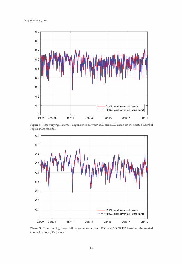
Energies 2020, 13, 1179

Figure 4. Time varying lower tail dependence between ESG and ECO based on the rotated Gumbelcopula (GAS) model.

Figure 5. Time varying lower tail dependence between ESG and SPGTCED based on the rotatedGumbel copula (GAS) model.

109

Energies 2020, 13, 1179

Figure 6. Time varying lower tail dependence between ESG and ERIX based on the rotated Gumbelcopula (GAS) model.

3.4. Goodness-of-Fit Test

In order to carry out the goodness-of-fit test for both the constant and time varying copula models,Kolomogorov–Smirnov and Cramer–von Mises methods are used in this paper. For the time varyingcopula models, the standard residuals should be transformed via the Rosenblatt method. In these twotests, significant statistics indicate that the models based on the data are rejected. The results of thetests on the constant and time varying copula models are reported in Table 6.

In the normal copula models, only the estimations of the parametric method pass the test.For the Clayton copula, no estimation passes the GOF test. For the rotated Gumbel copula, onlyone semi-parametric case passes the GOF test. For the Student’s t copula, only two estimations insemi-parametric cases yielded good results.

In time varying copula models, the p-values in the parametric case are higher than those in thesemi-parametric case, although almost all combinations pass both copula models. Comparatively,time varying models under the GAS method offer a better fit for the data than that of the constantcopula models.

110

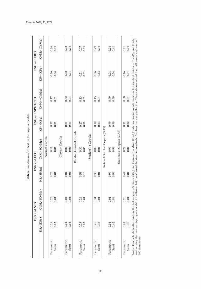
Energies 2020, 13, 1179

Ta

ble

6.

Goo

dnes

s-of

-fitt

esto

nth

eco

pula

mod

els.

ES

Ga

nd

NE

XE

SG

an

dE

CO

ES

Ga

nd

SP

GT

CE

DE

SG

an

dE

RIX

KS

C(K

SR

)C

vM

C(C

vM

R)

KS

C(K

SR

)C

vM

C(C

vM

R)

KS

C(K

SR

)C

vM

C(C

vM

R)

KS

C(K

SR

)C

vM

C(C

vM

R)

Nor

mal

Cop

ula

Para

met

ric

0.28

0.25

0.23

0.11

0.17

0.17

0.26

0.26

Sem

i0

.02

0.0

10

.01

0.0

10

.01

0.0

10

.04

0.0

1

Cla

yton

Cop

ula

Para

met

ric

0.0

10

.02

0.0

10

.04

0.0

10

.02

0.0

20

.02

Sem

i0

.01

0.0

10

.01

0.0

10

.01

0.0

10

.01

0.0

1

Rot

ated

Gum

belC

opul

a

Para

met

ric

0.28

0.21

0.58

0.30

0.27

0.13

0.21

0.07

Sem

i0

.02

0.0

10.

160

.03

0.0

10

.01

0.0

10

.01

Stud

ent’s

tCop

ula

Para

met

ric

0.26

0.34

0.35

0.09

0.10

0.15

0.36

0.29

Sem

i0.

030

.01

0.0

10

.01

0.0

30

.01

0.13

0.0

1

Rot

ated

Gum

belC

opul

a(G

AS)

Para

met

ric

0.0

10

.01

0.99

0.99

0.99

0.99

0.0

10

.01

Sem

i0.

420.

860.

990.

990.

990.

990.

540.

41

Stud

ent’s

tCop

ula

(GA

S)

Para

met

ric

0.41

0.20

0.47

0.22

0.11

0.08

0.16

0.21

Sem

i0.

060

.01

0.0

10

.01

0.0

20

.01

0.0

10

.01

Not

es:T

his

tabl

esh

ows

the

resu

lts

ofth

eK

olom

ogor

ov–S

mir

nov(K

S C)a

ndC

ram

er–v

onM

ises

(CvM

C)t

ests

onco

nsta

ntco

pula

mod

els

ofth

est

anda

rdre

sidu

als.

The

KS R

and

CvM

Rm

etho

ds

test

the

tim

eva

ryin

gco

pula

mod

elof

the

Ros

enbl

attt

rans

form

ofth

est

and

ard

resi

dua

ls.P

-val

ues

that

are

smal

ler

than

5%ar

esh

own

inbo

ldfo

nt.A

llre

sult

sar

eba

sed

on10

0si

mul

atio

ns.

111

Energies 2020, 13, 1179

4. Portfolio Performance

As shown above, we combine the ESG index with each of the renewable energy stock indices toform pairs and study their dependence structures. We further regard each pair of financial assets asa portfolio, each with different weights. By analyzing the traditional performance standards, suchas risk adjusted returns and value-at-risk (VaR), market participators investing in renewable energyindex funds and ESG can evaluate the potential revenues and stability behind each portfolio. Wedenote the portfolios between the ESG index and the renewable energy index as: ESG-NEX, ESG-ECO,ESG-SPGTCED, and ESG-EIRX. In this section, the skew t model and rotated Gumbel copula modelwill be used to estimate marginal distributions and dynamic dependence. In order to observe theperformance of two financial assets, we first need to obtain the linear correlation so we can calculatethe covariance and hence the portfolio variance. We simulated the correlation between the two returnsusing the copula parameters, as shown in Equation (8). Rather than analytically obtaining the results,we used a simulation based on the work by Patton [24].

ρt ≡ Corrt−1(Yu1,t, Yu2,t) = Corrt−1(ηu1,t, ηu2,t)

= Et−1(ηu1,t, ηu2,t) = Et−1(F−1

u1 (Uu1,t), F−1u2 (Uu2,t)

) (8)

where u1 and u2 denote different series.We consider three types of weights for two financial assets. In this research, we denote ω(i)1,t as the

ith type of weight in the ESG and ω(i)2,t(= 1−ω(i)1,t) as the weight in the renewable energy stock indexat time t. It is assumed that there is no transaction cost, so frequent changes in dynamic weights areallowed and will not affect the returns. The first method involves allocating a constant weight ω(1)1,t inthe ESG index. We regard the portfolio as a ‘static portfolio’. The second method (Equation (9)) iscalled ‘diversified risk-parity’, which provides greater capital in assets with less volatility. The thirdmethod (Equation (10)) is to consider the method developed by Kroner and Ng [30], which we regardas the ‘optimal portfolio’. The latter two dynamic weights are calculated based on conditional varianceand covariance.

ω(2)1,t = h22,t/(h11,t + h22,t) (9)

ω(3)1,t = (h22,t − h12,t)/(h11,t + h22,t − 2× h12,t)

(i f ω(3)1,t < 0, ω(3)1,t 0 i f ω(3)1,t >1, ω(3)1,t 1).(10)

The potential performances, including conditional returns, variance, value-at-risk (VaR),and conditional value-at-risk (CVaR, which is also called as expected shortfall (ES)), are obtained basedon the following steps. The portfolio contains two assets, denoted as u1 and u2.

1. We generate dynamic rotated Gumbel copula parameters{γt

}t=1,2,...,T based on the estimated time

varying pattern.2. For time t from 1 to T (total sample size), we generate uniform distributions for two targets Uu1,t

and Uu2,t using γt for S (= 5000) times, and hence the simulated standard residuals and returnsbased on the estimated marginal distribution parameters. Each element in marginal distributionsat time t is stored in a vector of size S× 1.

3. For time t, the portfolio returns are calculated based on each asset return and weight. For assetreturns of size S× 1, a lower qth quantile (we selected 1%, indicating a confidence level of 99% forVaR) is regarded as the VaR (Equation (11)). CVaR can also be obtained (Equation (12)).

VaRqt ≡ F−1

t (q), q ∈ (0, 1) (11)

CVaRqt ≡ E

[Yt

∣∣∣Ft−1, Yt ≤ VaRqt

], q ∈ (0, 1). (12)

112

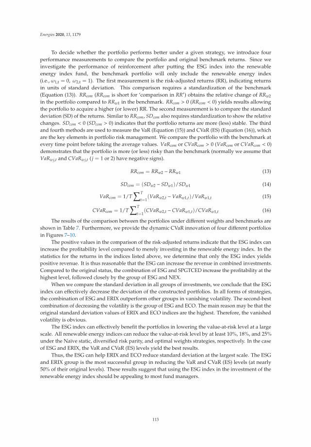
Energies 2020, 13, 1179

To decide whether the portfolio performs better under a given strategy, we introduce fourperformance measurements to compare the portfolio and original benchmark returns. Since weinvestigate the performance of reinforcement after putting the ESG index into the renewableenergy index fund, the benchmark portfolio will only include the renewable energy index(i.e., ω1,t = 0, ω2,t = 1). The first measurement is the risk-adjusted returns (RR), indicating returnsin units of standard deviation. This comparison requires a standardization of the benchmark(Equation (13)). RRcom (RRcom is short for ‘comparison in RR′) obtains the relative change of RRw2

in the portfolio compared to RRw1 in the benchmark. RRcom > 0 (RRcom < 0) yields results allowingthe portfolio to acquire a higher (or lower) RR. The second measurement is to compare the standarddeviation (SD) of the returns. Similar to RRcom, SDcom also requires standardization to show the relativechanges. SDcom < 0 (SDcom > 0) indicates that the portfolio returns are more (less) stable. The thirdand fourth methods are used to measure the VaR (Equation (15)) and CVaR (ES) (Equation (16)), whichare the key elements in portfolio risk management. We compare the portfolio with the benchmark atevery time point before taking the average values. VaRcom or CVaRcom > 0 (VaRcom or CVaRcom < 0)demonstrates that the portfolio is more (or less) risky than the benchmark (normally we assume thatVaRwj,t and CVaRwj,t ( j = 1 or 2) have negative signs).

RRcom = RRw2 −RRw1 (13)

SDcom = (SDw2 − SDw1)/SDw1 (14)

VaRcom = 1/T∑T

t=1(VaRw2,t −VaRw1,t)/VaRw1,t (15)

CVaRcom = 1/T∑T

t=1(CVaRw2,t −CVaRw1,t)/CVaRw1,t (16)

The results of the comparison between the portfolios under different weights and benchmarks areshown in Table 7. Furthermore, we provide the dynamic CVaR innovation of four different portfoliosin Figures 7–10.

The positive values in the comparison of the risk-adjusted returns indicate that the ESG index canincrease the profitability level compared to merely investing in the renewable energy index. In thestatistics for the returns in the indices listed above, we determine that only the ESG index yieldspositive revenue. It is thus reasonable that the ESG can increase the revenue in combined investments.Compared to the original status, the combination of ESG and SPGTCED increase the profitability at thehighest level, followed closely by the group of ESG and NEX.

When we compare the standard deviation in all groups of investments, we conclude that the ESGindex can effectively decrease the deviation of the constructed portfolios. In all forms of strategies,the combination of ESG and ERIX outperform other groups in vanishing volatility. The second-bestcombination of decreasing the volatility is the group of ESG and ECO. The main reason may be that theoriginal standard deviation values of ERIX and ECO indices are the highest. Therefore, the vanishedvolatility is obvious.

The ESG index can effectively benefit the portfolios in lowering the value-at-risk level at a largescale. All renewable energy indices can reduce the value-at-risk level by at least 10%, 18%, and 25%under the Naïve static, diversified risk parity, and optimal weights strategies, respectively. In the caseof ESG and ERIX, the VaR and CVaR (ES) levels yield the best results.

Thus, the ESG can help ERIX and ECO reduce standard deviation at the largest scale. The ESGand ERIX group is the most successful group in reducing the VaR and CVaR (ES) levels (at nearly50% of their original levels). These results suggest that using the ESG index in the investment of therenewable energy index should be appealing to most fund managers.

113

Energies 2020, 13, 1179

Table 7. Portfolio performance comparison.

Strategy Measure ESG and NEX ESG and ECO ESG and SPGTCED ESG and ERIX

Naïve Static

RRcom 0.0118 0.0106 0.0130 0.0078SDcom −0.1672 −0.2871 −0.2640 −0.2976

VaRcom −0.1404 −0.2680 −0.2406 −0.2851

CVaRcom −0.1364 −0.2562 −0.2070 −0.2770

Diversified riskparity

RRcom 0.0167 0.0237 0.0254 0.0159SDcom −0.2066 −0.4189 −0.3777 −0.4316

VaRcom −0.1852 −0.4244 −0.3379 −0.4460

CVaRcom −0.1801 −0.4039 −0.2986 −0.4305

Optimalweights

RRcom 0.0291 0.0345 0.0403 0.0267SDcom −0.2722 −0.4890 −0.4502 −0.4957

VaRcom −0.2501 −0.4964 −0.4052 −0.5084

CVaRcom −0.2389 −0.4712 −0.3615 −0.4903

Notes: In this table, four comparative measurements of the performance between each portfolio and benchmarkare reported. For the Naïve Static strategy, we only report the equally (50% to 50%) weighted examples. In eachstrategy, we report the best results in each row for SDcom, VaRcom, and EScom in bold font.

(a) (b)

Figure 7. Time varying conditional value-at-risk (CVaR) between the ESG and NEX portfolios ((a) is theCVaR under the ‘naïve static’ strategy; (b) is the CVaR under the ‘diversified risk parity’ and ‘optimalweights’ strategies).

(a) (b)

Figure 8. Time varying CVaR between the ESG and ECO portfolios ((a) is the CVaR under the ‘naïvestatic’ strategy; (b) is the CVaR under the ‘diversified risk parity’ and ‘optimal weights’ strategies).

114

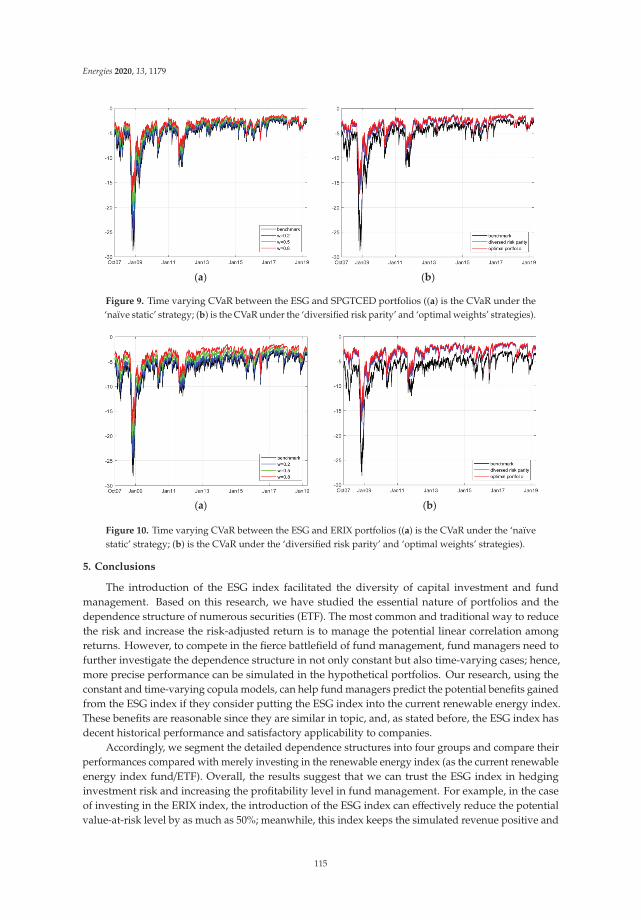
Energies 2020, 13, 1179

(a) (b)

Figure 9. Time varying CVaR between the ESG and SPGTCED portfolios ((a) is the CVaR under the‘naïve static’ strategy; (b) is the CVaR under the ‘diversified risk parity’ and ‘optimal weights’ strategies).

(a) (b)

Figure 10. Time varying CVaR between the ESG and ERIX portfolios ((a) is the CVaR under the ‘naïvestatic’ strategy; (b) is the CVaR under the ‘diversified risk parity’ and ‘optimal weights’ strategies).

5. Conclusions

The introduction of the ESG index facilitated the diversity of capital investment and fundmanagement. Based on this research, we have studied the essential nature of portfolios and thedependence structure of numerous securities (ETF). The most common and traditional way to reducethe risk and increase the risk-adjusted return is to manage the potential linear correlation amongreturns. However, to compete in the fierce battlefield of fund management, fund managers need tofurther investigate the dependence structure in not only constant but also time-varying cases; hence,more precise performance can be simulated in the hypothetical portfolios. Our research, using theconstant and time-varying copula models, can help fund managers predict the potential benefits gainedfrom the ESG index if they consider putting the ESG index into the current renewable energy index.These benefits are reasonable since they are similar in topic, and, as stated before, the ESG index hasdecent historical performance and satisfactory applicability to companies.

Accordingly, we segment the detailed dependence structures into four groups and compare theirperformances compared with merely investing in the renewable energy index (as the current renewableenergy index fund/ETF). Overall, the results suggest that we can trust the ESG index in hedginginvestment risk and increasing the profitability level in fund management. For example, in the caseof investing in the ERIX index, the introduction of the ESG index can effectively reduce the potentialvalue-at-risk level by as much as 50%; meanwhile, this index keeps the simulated revenue positive and

115

Energies 2020, 13, 1179

more stable. During huge losses, such as the 2008 and 2011 crises, the time varying CVaR graphs revealthat balancing the renewable energy index with the ESG index can be helpful in reducing large losses.

Author Contributions: Conceptualization, S.H.; investigation, G.L.; writing—original draft preparation, G.L.;writing—review and editing, S.H.; project administration, S.H.; funding acquisition, S.H. All authors have readand agreed to the published version of the manuscript.

Funding: This work was supported by JSPS KAKENHI, grant number 17H00983.

Acknowledgments: We are grateful to three anonymous referees for their helpful comments and suggestions.


Appendix A

Table A1. Portfolio cointegration and Granger causality test (p-value).

Tests ESG and NEX ESG and ECO ESG and SPGTCED ESG and ERIX

Cointegration (index) 0.9659 0.8583 0.8763 0.9660ESG → others (returns) 0.0001 0.0102 0.0702 0.0001ESG ← others (returns) 0.0001 0.0001 0.0111 0.0001

Notes: In this table, four pairs of index and returns are tested in Engle–Granger cointegration and causality.The maximum lag is set as 5. In the Granger causality test, A → B implies that A is the Granger cause of B, vise verse.We test the cointegration on originally daily index values, while testing the Granger causality on daily returns.

References

1. Tang, D.Y.; Zhang, Y. Do shareholders benefit from green bonds? J. Corp. Financ. 2018. [CrossRef]2. Klassen, R.; McLaughlin, C. The impact of environmental management on frm performance. Manag. Sci.

1996, 42, 1199–1214. [CrossRef]3. Mello, A.S.; Parsons, J.E. Hedging and Liquidity. Rev. Financ. Stud. 2000, 13, 127–153. [CrossRef]4. Lins, K.V.; Servaes, H.; Tufano, P. What drives corporate liquidity? An international survey of cash holdings

and lines of credit. J. Financ. Econ. 2010, 98, 160–176. [CrossRef]5. Shin, Y.J.; Pyo, U. Liquidity Hedging with Futures and Forward Contracts. Stud. Econ. Financ. 2019, 36,

265–290. [CrossRef]6. Kaminker, C.; Stewart, F. “The Role of Institutional Investors in Financing Clean Energy OECD Working

Papers on Finance, Insurance and Private Pensions, No.23, OECD Publishing.” 23. OECD Working Paperson Finance, Insurance and Private Pensions. 2012. Available online: www.oecd.org/daf/fin/wp (accessed on1 September 2019).

7. Dimson, E.; Karakas, O.; Li, X. Active ownership. Rev. Financ. Stud. 2015, 28, 3225–3268. [CrossRef]8. Hoepner, A.; Oikonomou, I.; Sautner, Z.; Starks, L.; Zhou, X. ESG Shareholder Engagement and Downside

Risk. Unpublished work. 2018.9. Sultana, S.; Zulkifli, N.; Zainal, D. Environmental, Social and Governance (ESG) and Investment Decision in

Bangladesh. Sustainability 2018, 10, 1831. [CrossRef]10. Keppler, J.H.; Mansanet-Bataller, M. Causalities between CO2, electricity, and other energy variables during

phase I and phase II of the EU ETS. Energy Policy 2010, 38, 3329–3341. [CrossRef]11. Reboredo, J.C.; Rivera-Castro, M.A.; Ugolini, A. Wavelet-based test of co-movement and causality between

oil and renewable energy stock prices. Energy Econ. 2017, 61, 241–252. [CrossRef]12. Reboredo, J.C. Is there dependence and systemic risk between oil and renewable energy stock prices? Energy

Econ. 2015, 48, 32–45. [CrossRef]13. Rockafellar, R.T.; Uryasev, S. Optimization of Conditional Value-at-Risk. J. Risk 2000, 2, 21–41. [CrossRef]14. Pflug, G.C. Some remarks on the value-at-risk and the conditional value-at-risk. In Probabilistic Constrained

Optimization; Springer: Boston, MA, USA, 2000; pp. 272–281.15. Artzner, P.; Delbaen, F.; Eber, J.M.; Heath, D. Coherent measures of risk. Math. Financ. 1999, 9, 203–228.

[CrossRef]16. Deng, L.; Ma, C.; Yang, W. Portfolio optimization via pair copula-GARCH-EVT-CVaR model. Syst. Eng.

Procedia 2011, 2, 171–181. [CrossRef]

116

Energies 2020, 13, 1179

17. He, X.; Gong, P. Measuring the coupled risks: A copula-based CVaR model. J. Comput. Appl. Math. 2009, 223,1066–1080. [CrossRef]

18. Fama, E.F. The behavior of stock-market prices. J. Bus. 1965, 38, 34–105. [CrossRef]19. Hsu, D.A.; Miller, R.B.; Wichern, D.W. On the stable Paretian behavior of stock-market prices. J. Am. Stat.

Assoc. 1974, 69, 108–113. [CrossRef]20. Mantegna, R.N.; Stanley, H.E. Introduction to Econophysics: Correlations and Complexity in Finance; Cambridge

University Press: Cambridge, UK, 2000.21. Figueiredo, A.; Gleria, I.; Matsushita, R.; Da Silva, S. On the origins of truncated Lévy flights. Phys. Lett. A

2003, 315, 51–60. [CrossRef]22. Yang, L.; Hamori, S. Dependence structure among international stock markets: A GARCH-copula analysis.

Appl. Financ. Econ. 2013, 23, 1805–1817. [CrossRef]23. Yang, L.; Hamori, S. Dependence Structure between CEEC-3 and German Government Securities Markets. J.

Int. Financ. Mark. Inst. Money 2014, 29, 109–125. [CrossRef]24. Patton, A. Copula methods for forecasting multivariate time series. In Handbook of Economic Forecasting;

Elsevier: Amsterdam, The Netherlands, 2013; Volume 2, pp. 899–960. [CrossRef]25. Hansen, B.E. Autoregressive conditional density estimation. Int. Econ. Rev. 1994, 35, 705–730. [CrossRef]26. Genest, C.; Rémillard, B. Validity of the parametric bootstrap for goodness-of-fit testing in semiparametric

models. In Annales de l’Institut Henri Poincaré, Probabilités et Statistiques; Institut Henri Poincaré: Paris, France,2008; Volume 44, pp. 1096–1127.

27. Sklar, M. Fonctions de répartition à n dimensions et leurs marges. Publ. l’Inst. Stat. l’Univ. Paris 1959, 8,229–231.

28. Gumbel, E.J. Bivariate exponential distributions. J. Am. Stat. Assoc. 1960, 55, 698–707. [CrossRef]29. Creal, D.; Koopman, S.J.; Lucas, A. Generalized autoregressive score models with applications. J. Appl.

Econom. 2013, 28, 777–795. [CrossRef]30. Kroner, K.F.; Ng, V.K. Modeling asymmetric comovements of asset returns. Rev. Financ. Stud. 1998, 11,

817–844. [CrossRef]


117

energies

Article

How Does the Spillover among Natural Gas, CrudeOil, and Electricity Utility Stocks Change over Time?Evidence from North America and Europe

Wenting Zhang 1, Xie He 1, Tadahiro Nakajima 1,2 and Shigeyuki Hamori 1,*

1 Graduate School of Economics, Kobe University, 2-1 Rokkodai, Nada-Ku, Kobe 657-8501, Japan;[email protected] (W.Z.); [email protected] (X.H.);[email protected] (T.N.)

2 The Kansai Electric Power Company, Incorporated, 3-chome-6-16 Nakanoshima, Kita-Ku,Osaka 530-8270, Japan

* Correspondence: [email protected]

Received: 7 January 2020; Accepted: 2 February 2020; Published: 7 February 2020

Abstract: Our study analyzes the return and volatility spillover among the natural gas, crude oil, andelectricity utility stock indices in North America and Europe from 4 August 2009 to 16 August 2019.First, in time domain, both total return and volatility spillover are stronger in Europe than in NorthAmerica. Furthermore, compared to natural gas, crude oil has a greater volatility spillover on theelectricity utility stock indices in North America and Europe. Second, in frequency domain, mostof the return spillover occurs in the short-term, while most of the volatility spillover occurs over alonger period. Third, the rolling analyses indicate that the return and volatility from 2009 to late 2013remained stable in North America and Europe, which may be a result of the 2008 global financialcrisis, and started to fluctuate after late 2013 due to some extreme events, indicating that extremeevents can significantly influence spillover effects. Moreover, investors should monitor current eventsto diversify their portfolios properly and hedge their risks.

Keywords: natural gas; crude oil; electricity utilities sector index; spillover effect;time–frequency dynamics

1. Introduction

Our paper is aimed at analyzing the return and volatility spillover among natural gas, crudeoil, and the electricity utility sector indices across North America and Europe using the methodsof Diebold and Yilmaz [1] and Barunik and Krehlik [2] in time and frequency domains. In currentcommodity markets, energy futures play a major role in economic activities. In particular, as naturalgas is cleaner and produces fewer greenhouse emissions than fossil fuels, such as oil and coal, theimportance of natural gas has been increasing in the global energy market. Natural gas can be usedin many areas, including residential, commercial, industrial, power generation, and vehicle fuels.According to the IEA, natural gas grew 4.6% in 2018, accounting for almost half of the increase in globalenergy demands (https://www.iea.org/fuels-and-technologies/gas). In both national policy scenarios(gas demand increases by more than a third) and sustainable development scenarios (gas demand willincrease slowly by 2030 and return to current levels by 2040), natural gas continues to outperform coaland oil. Meanwhile, crude oil is used to generate electricity, which is also an important raw materialfor the chemical industry. Thus, we chose the United States (US) and Canada in North America, andGermany, France, the United Kingdom (UK), and Italy in Europe, which are the Group of Seven (G7)member countries, to investigate the spillover among the two energies and electricity utility stocks.According to the BP Statistical Review of World Energy 2019 [3], the consumption shares of natural gas


Energies 2020, 13, 727

and crude oil in 2018 were as follows: US (16.6%), Canada (2.5%), Germany (2.3%), France (1.7%), theUK (1.4%), and Italy (1.1%). These six countries are major consumers of natural gas and crude oil.

With the development of financial globalization, the financial community is paying increasinglymore attention to the transmission of dynamic return links and volatility throughout the capital market.In the situation of a market crash or crisis, portfolio managers and policymakers need to take someactions to prevent the risk of transmission. Therefore, empirical research on the intensity of spilloversprovides insights for accurate predictions of returns and volatility. In particular, investors shouldknow, especially in recent years, how fluctuations in natural gas, crude oil, and electricity utilitiesstock indices affect the risk and value of their investment portfolios. In addition, from 2009 to 2019,several major events influenced these two energy markets and the stock market. These extreme eventsled to fluctuations in the return and volatility spillover among the three markets in North Americaand Europe. Hence, understanding the return and volatility spillover caused by financial shocks isnot only essential for investors in terms of risk management and portfolio diversification but also forpolicymakers in developing appropriate policies to avoid impacts from future extreme events. Tianand Hamori [4] have also indicated that policymakers need to understand the transmission mechanismof volatility shock spillover that leads to financial instability.

The main contributions of our study can be summarized as follows. First, as far as we know, thisis the first study to investigate the return and volatility spillover among natural gas, crude oil, andthe electricity utility sector indices in North America and Europe, respectively, using the Diebold andYilmaz [1] method for time domain and the Barunik and Krehlik [2] method for frequency domain.Second, we separately analyzed the return and volatility spillover in North America and Europebetween the two energy futures and electricity utility stocks to determine the similarities and differencesof the spillover effects in the two regions. Third, we employ a rolling analysis to examine the dynamicsof the connectedness of return and volatility in time and frequency domains.

The remainder of our paper is described as follows. Section 2 provides a literature review. Section 3describes the empirical techniques. In Section 4, we explain the data and the descriptive statisticsthrough a preliminary analysis. In Section 5, we report the empirical results of the spillover effects andthe moving window analysis. Finally, we conclude our analysis in Section 6.


There are numerous studies in the literature investigating spillover effects on the relationshipbetween crude oil and stock markets. Arouri et al. [5] used the generalized vector autoregression(VAR)–generalized autoregressive conditional heteroskedasticity (GARCH) model to analyze thevolatility spillover between oil and the stock markets in Europe and the US. Using the sector data, theyfound that oil and sector stock returns have significant volatility spillover. Soytas and Oran [6] usedthe Cheung–Ng approach (Cheung and Ng [7]) to analyze the volatility spillover between the worldoil market and electricity stock returns in Turkey. They found new information that was not foundthrough conventional causality tests using aggregated market indices. Arouri et al. [8] used a recentgeneralized VAR–GARCH model to investigate the return and volatility spillover between the oil andstock markets among Gulf Cooperation Council (GCC) countries from 2005 to 2010. They found thatthe return and volatility spillover between them was significant enough for investors to diversify theirportfolios. Nazlioglus et al. [9] investigated the volatility transmission between crude oil and someagricultural commodity markets (wheat, corn, soybean, and sugar). They found that the good pricecrisis and risk transmission has significantly affected the dynamics of volatility spillover. Nakajimaand Hamori [10] analyzed the relationship among electricity prices, crude oil prices, and exchangerates. They found that exchange rates and crude oil Granger cause electricity prices neither in meannor in variance.

Despite the many well-documented studies on the spillover between crude oil and the stockmarket, there are relatively few studies on the natural gas and financial markets. Ewing et al. [11]analyzed the volatility spillover between oil and natural gas markets using the GARCH model.

120

Energies 2020, 13, 727

Acaravci et al. [12] investigated the long-term relationship between natural gas prices and stock pricesusing the vector error correction model developed by Johansen and Juselius [13].

Diebold and Yilmaz [1,14,15] developed the methodology of analyzing the connectedness in timedomain based on the variance decomposition of the forecast error to assess the share of forecast errorvariation in its magnitude and direction; Barunik and Krehlik [2] then extended this connectedness tofrequency domain to show the spillover effect from different frequency ranges. Many researchers haveapplied these empirical techniques to investigate the connectedness between markets in time domainor both in time and frequency domains.

Maghyereh et al. [16] analyzed the connectedness between oil and equities in 11 major stockexchanges in time domain. They found a robust transmission from the crude oil market to the equitymarket, which grew stronger from mid-2009 to mid-2012. Duncan and Kabundi [17] investigatedthe domestic and foreign sources of volatility spillover in South Africa in time domain. In addition,Liow [18] characterized the conditional volatility spillover among G7 countries in regard to publicreal estate, stocks, bonds, money, and currency, both domestically and internationally in time domain.Sugimoto et al. [19] examined the spillover effects on African stock markets during the global financialcrisis and the European sovereign debt crisis in time domain.

Toyoshima and Hamori [20] researched the connectedness of return and volatility in the globalcrude oil markets in time and frequency domains. They found that the Asian currency crisis (1997–1998)and the global financial crisis (2007–2008) generated an increase in return and volatility spillover effects.Lovcha et al. [21] characterized the dynamic connectedness between oil and natural gas volatility infrequency domain. Ferrer et al. [22] analyzed the return and volatility connectedness of the stockprices of US clean energy companies, crude oil prices, and important financial variables in time andfrequency domains.

We use a rolling analysis to examine the spillover of return and volatility in North America andEurope separately in time and frequency domains. Zhang and Wang [23] also analyzed the returnand volatility spillover between the Chinese and global oil markets and employed a moving-windowanalysis to better understand and capture the dynamics of return and volatility spillover in time domain.

Finally, we investigate some prior studies similar to ours. Similar to our study, Oberndorferet al. [24] focused on investigating the volatility spillover across energy markets and the pricing ofEuropean energy stocks by using the GARCH model, and they found that oil price is the main indexfor energy price developments in the European stock market. Kenourgios et al. [25] investigated thecontagion effects of the global financial crisis (2007–2009) across assets in different regions. Kenourgioset al. [26] also investigated the contagion effects of the global financial crisis (2007–2009) in six developedand emerging regions by applying the FIAPARCH model. Baur [27] also studied different channelsof financial contagions across 25 major countries and found that the crisis significantly increased theco-movement of returns. Singh et al. [28] examined price and volatility spillovers in the stock marketsof North America, Asia, and Europe and found that a greater regional influence exists among the Asianand European stock markets. Balli et al. [29] analyzed the return and volatility spillovers and theirdeterminants in emerging Asian and Middle Eastern countries. They found that developed financialmarkets have significant spillover effects on emerging financial markets and shocks originated in theUS play a dominant role.

3. Empirical Techniques

3.1. Diebold–Yilmaz Method

Our study employs the method proposed by Diebold and Yilmaz [1] for measuring spillover in ageneralized VAR framework. This approach was designed to measure the connectedness concept built

121

Energies 2020, 13, 727

on the basis of the generalized forecast error variance decomposition (GFEVD) of a VAR approximatingmodel. First, we conceived an N-variable VAR (p) model, as (1) below.

yt=∑p

i=1Φiyt−i+εt (1)

where yt is the N × 1 vector of the observed variables at time t, and Φ is the N × N coefficient matrix.The error vector εt is independent and identically distributed, and white noise (0,

∑) with covariance

matrix∑

is possibly non-diagonal.In this model, the VAR process can also transform into the vector moving average (VMA) (∞), as

represented in (2). It is effective to use with the (N × N) matrix lag-polynomial |In-Φ1z−· · · −Φpzp| = 0with the In identity matrix. Assuming that the roots of |Φ(z)| lie outside the unit circle,

yt=ψ(L)εt (2)

where ψ(L) is the (N × N) matrix of infinite lag polynomials that can be calculated from ψ(L) =[ψ(L)]−1. However, as the order of the variables in the VAR system may influence the impulse responseor variance decomposition results, to eliminate the influence from the ordering of the variables in thevariance decomposition, Diebold and Yilmaz [1] applied the generalized VAR framework developed byKoop et al. [30] and Pesaran and Shin [31]. On the basis of this framework, the H-step-ahead GFEVDcan be written in the form of (3):

(θH) jk =σ−1

kk ΣHh=0((ψhΣ) jk)

2

ΣHh=0(ψhΣψ

′h) j j

(3)

where ψh is an N × N coefficient matrix of polynomials at lag h, and σ−1kk = (Σ)kk. (θH) jk indicates the

contribution of the kth variable of the model to the variance of the forecast error of element j at horizonh. To sum the elements in each row of the GFEVD to total 1, each entry is normalized by the row sum as

~θ

H

jk =θH

jk

ΣNK=1θ

Hjk

(4)

~θ

H

jk measures the pairwise spillover from k to j at horizon H and also measures the spillover effect frommarket k to j. We can aggregate this to measure the total spillover of the system. The total spillover canbe measured by the pairwise spillover. The connectedness can be seen as the share of variance in theforecasts contributed to by errors (Diebold and Yilmaz [1]).

SH = 100×ΣN

j�k

~θ

H

jk

Σ~θ

H = 100×

⎛⎜⎜⎜⎜⎜⎜⎜⎜⎜⎜⎜⎜⎜⎝1−Tr

{~θ

H}

Σ~θ

H

⎞⎟⎟⎟⎟⎟⎟⎟⎟⎟⎟⎟⎟⎟⎠ = 100×

⎛⎜⎜⎜⎜⎜⎜⎜⎜⎜⎜⎜⎜⎜⎝1−Tr

{~θ

H}

N

⎞⎟⎟⎟⎟⎟⎟⎟⎟⎟⎟⎟⎟⎟⎠ (5)

where Tr{.} is the trace operator. The total spillover calculates the total spillover across all markets inthe form of (5). There are two measures by Diebold and Yilmaz [1] that show the relative importanceof each variable in the system:

Directional Spillover (From): SHk← = 100× ; the directional spillover (from) is the spillover

that market k receives from all other markets.

Directional Spillover (To): SH←k = 100× ; the directional spillover (to) is the spillover that

market k transmits to all other markets.

122

Energies 2020, 13, 727

3.2. Barunik and Krehlik Method

Following Barunik and Krehlik [2], we describe the frequency dynamics (for the short-term, themedium-term, and the long-term) of spillover and the spectral formulation of variance decomposition.

Notably, we measure spillovers in frequency domain using Fourier transform. Moreover, thefrequency response function is obtained as a Fourier transform of the coefficients ψh:ψ

(e−iω

)=

Σhe−iωhψh, where i =√−1. The generalized causation spectrum over frequenciesω ∈ (−π, π) is defined

in the form of (6)

( f (ω)) jk =

σ−1kk

∣∣∣∣∣(ψ(e−iω)Σ)

jk

∣∣∣∣∣2(ψ(e−iω)Σψ′(e+iω)) j j

(6)

where ψ(e−iω

)= Σhe−iωhψh is the Fourier transform of the impulse response ψh. It is vital to pay

attention to (f(ω)) jk, namely, the portion of the spectrum of the jth variable at a given frequency ωdue to shocks in the kth variable. As domination holds the spectrum of the jth variable at a givenfrequency ω, we establish (6) for the quantity within the frequency causation. To obtain the generalizeddecomposition of the variance’s decompositions to frequencies, we weight (f(ω)) jk by the frequencyshare of the variance of the jth variable. This weighting function can be defined as (7)

Γ j(ω) =(ψ

(e−iω

)Σψ′

(e+iω

))

j j

12π

∫ π−π(ψ(e−iλ)Σψ′(e+iλ)) j jdλ

(7)

where the power of the jth variable at a given frequency sums through the frequencies to a constantvalue of 2π. When the Fourier transform of the impulse is a complex number value, the generalizedfactor spectrum is the squared coefficient of the weighted complex numbers and, therefore, a realnumber. In sum, we set the frequency band d = (a, b): a, b ∈ (−π, π), a < b.

The GFEVD under the frequency band d is

θjk(d) =1

2π

∫ b

aΓ j(ω)(f(ω)) jkdω (8)

However, GFEVD will still be normalized into (9). The scaled GFEVD on the frequency band d =(a, b): a, b ∈ (−π, π), a < b is shown below:

~θjk(d) =

θjk(d)

Σkθjk(∞)(9)

where~θ jk(d) is defined as the pairwise spillover at a given frequency band d. At the same time, it is

possible to define the total spillover at frequency band d.The frequency total spillover (frequency connectedness) on frequency band d can be defined as

SF(d) = 100×⎛⎜⎜⎜⎜⎜⎜⎜⎜⎜⎝ Σ

~θ(d)

Σ~θ(∞)

−Tr

{~θ(d)

}Σ

~θ(∞)

⎞⎟⎟⎟⎟⎟⎟⎟⎟⎟⎠ (10)

where Tr{.} is the trace operator, and Σ~θ(d) is the sum of all elements of the

~θ(d) matrix. The frequency

total spillover decomposes the total spillover into the long-term, the medium-term, and the short-term,and these can sum into the total spillover S, as defined by Diebold and Yilmaz [1].

Equally, we can also define the two directional spillovers for frequency according to Diebold andYilmaz [1].

123

Energies 2020, 13, 727

Frequency Directional Spillover (From): SFk←(d) = 100 × ; the frequency directional

spillover (from) is the spillover that market k receives from all other markets at frequency band d.

Frequency Directional Spillover (To): SH←k(d) = 100× ; the frequency directional spillover

(to) is the spillover that market k transmits to all other markets at frequency band d.

4. Data

We use daily data for the natural gas, crude oil, and electricity utility sector indices of Europe andNorth America from 4 August 2009 to 16 August 2019, without uncommon business days. Becausethe data and CAC Utilities Index (USD) extends from 4 August 2009 to 16 August 2019, in order toconsolidate the time for all data, we chose this time period. To avoid the influence of the exchangerate on our results, we consolidated the currency units of the variables into a dollar currency unit.Specifically, the variables we use are shown in Table 1.


North America


Natural Gas Henry Hub Natural Gas Futures (USD/Million Btu) BloombergCrude Oil Crude Oil WTI Futures (USD/Barrel) Bloomberg

US S&P 500 Utilities Index (USD) Dow JonesCanada S&P/TSX Capped Utilities Sector Index (USD) Bloomberg

Europe


Natural Gas ICE UK Natural Gas Futures (NBP) (USD/Million Btu) BloombergCrude Oil ICE Brent Futures (USD/Barrel) BloombergGermany DAX subsector All Electricity (USD) DataStream

UK FTSE 350 Electricity Index (USD) DataStreamFrance CAC Utilities Index (USD) DataStreamItaly FTSE ITALIA ALL-SHARE UTILITIES (USD) DataStream

For the North American market, we use the daily prices of the Henry Hub Natural Gas Futuresfrom Bloomberg for the natural gas market. For the crude oil market, we employ the Crude Oil WTIFutures from Bloomberg. With exports grown in Europe, South America, and Asia, the New YorkMercantile Exchange (NYMEX) Henry Hub Natural Gas futures have become a global price benchmarkfor natural gas trading. WTI, a medium crude oil and futures contract launched by the NYMEX in 1983,has long been a benchmark for international crude oil prices, thus making an important contributionto the development of the global crude oil market. For the stock market, we use the electricity utilitiesin the US and Canada. For the US, we use the Standard and Poors 500 Utilities (S&P 500) which iscomposed of electricity and energy companies included in the S&P 500. This is classified as membersof the Global Industry Classification Standard (GICS) utilities sector, such as the American ElectricPower Company (AEP), Duke Energy Company (DU), Consolidated Edison Company (ED), and 28other companies in total. The S&P/TSX Capped Utilities Sector Index (TSX) is a market-value-weightedindex obtained from 16 electricity and energy companies, such as Emera Inc. (EMA) and Fortis Inc.(FTS).

For Europe, we use the daily price of the Intercontinental Exchange (ICE) UK Natural Gas Futuresfor the natural gas market and the ICE Brent Futures for the crude oil market. The ICE UK Natural GasFutures contract is used for physical delivery by transfer of natural gas rights at the National BalancingPoint (NBP) virtual trading point operated by the National Grid, a UK transmission system operator.

124

Energies 2020, 13, 727

This is the second most common liquid gas trading point in Europe. Brent Oil is the primary tradingcategory for sweet light crude and serves as a benchmark price for oil purchases in the world. For stockmarkets, in Germany, we use the Dax subsector All Electricity (DAX), calculated by Deutsche Börse.DAX is a market-value-weighted index that includes companies with an average daily trading volumeof at least €1 million to qualify. In the UK, we use the market-value-weighted FTSE 350 Electricity Index(FTSE 350), which includes three companies: DRAXGROUP, SSE (Scottish and Southern Electricity),and Contour global, all of which are large electricity enterprises in the UK. In France, we use theCAC Utilities Index (CAC), a market-value-weighted index that comprises 10 electricity and energycompanies, including EDF and ENGIE. In Italy, we use the FTSE ITALIA ALL-SHARE UTILITIESIndex (FTSE Italia), which includes 14 electricity and energy companies, such as ENEL (an Italianmultinational energy company working in the field of power generation and distribution).

Figure 1a shows images of the prices of natural gas, crude oil, and the electricity utility sectorindices in North America. Figure 1b illustrates the natural gas, crude oil, and electricity utility sectorindices in Europe. As we can see, in the North America market, the price of the natural gas, crudeoil, and electricity utility sector index in Canada follow similar trends and fluctuate violently. Thesetrends dropped dramatically from 2014 to 2016 due to the international oil price crisis. In general,the electricity utility sector index in the US increased continuously from 2009 to 2019, after the globalfinancial crisis of 2007–2009. Relatively, in the European market, Figure 1b shows that the prices ofnatural gas, crude oil, and the electricity utility sector index follow a semblable non-stationary trend.Moreover, due to international oil price crisis of 2014–2016, energy prices dropped to varying degreesduring this time period.

In our analysis, we calculated the closing price of the North American market and the Europeanlogarithmic difference as the daily return data, as shown in Figure 2a,b. Furthermore, we use theLjung-Box, which has a lag of 20 to test the time variations of the return series and confirm thatthe return of all variables is not a white noise series with 10% significance. We use the ARMA(Autoregressive Moving Average)–GARCH model to calculate the volatilities of four assets in NorthAmerica and six assets in Europe, and the plots are shown in Figure 3a,b. Additionally, the lag of theGARCH model is determined on the basis of the Akaike Information Criterion (AIC).

The descriptive basic statistics of the return and volatility series are shown in Table 2, Table 3.In North America, we find that the mean returns of natural gas and crude oil have negative values.However, the others have positive mean returns. Furthermore, natural gas has the largest maximumdaily return and the largest minimum daily return. Specifically, we find that natural gas is the mostvolatile, followed by crude oil, TSX (Canada), and the S&P 500 (US). Moreover, based on skewness,we find that, except for natural gas, the returns are left-skewed, whereas the return of natural gas isright-skewed. Meanwhile, according to kurtosis, the volatility of the four assets are right-skewed.Regarding kurtosis, the returns and volatilities of the four assets are leptokurtic, which means thatthe four variables will show more peaked and fat tails. Finally, as the most commonly used unit roottesting method, the augmented Dickey–Fuller (ADF), proposed in 1981, tests the null hypothesis that avariable has a unit root, which means that the variable is nonstationary. From the ADF results, the nullhypothesis is rejected at 1% significance level for all variables.

125

Energies 2020, 13, 727

(a)

(b)

Figure 1. (a) Time-variations of the price series in North America. Notes: Henry Hub indicates naturalgas; WTI indicates crude oil; US indicates the S&P 500 Utilities Index; CANADA indicates the S&P/TSXCapped Utilities Sector Index. (b) Time-variations of the price series in Europe. Notes: NBP indicatesnatural gas; BRENT indicates crude oil; GERMANY indicates the DAX subsector for all electricity; UKindicates the FTSE 350 Electricity Index; FRANCE indicates the CAC Utilities Index; ITALY indicatesFTSE Italia All-Share Utilities Index.

Meanwhile, in the European market, in contrast to the North America market, we see that themean returns of crude oil, DAX (Germany), FTSE 350 (UK), and CAC (France) have negative values.However, the others have positive mean returns. Natural gas has the largest maximum daily return, andFTSE 350 (the UK) has the largest minimum daily return. However, we find that natural gas is the mostvolatile, followed by crude oil, DAX (Germany), CAC (France), FTSE Italia (Italy), FTSE 350 (UK), andDAX (Germany). On the basis of skewness, the returns of natural gas and crude oil are right-skewed,but the others are left-skewed. In addition, the volatilities of the six assets are right-skewed. Regardingkurtosis, except for the return of CAC (France), which is platykurtic, the returns of the others are

126

Energies 2020, 13, 727

leptokurtic. Moreover, the volatilities of the six assets are leptokurtic. Eventually, based on the ADFresults, we reject the null hypothesis of a unit root at 1% significance level for all series.

(a)

(b)

Figure 2. (a) Time-variations of the return series in North America. Notes: Henry Hub indicates naturalgas; WTI indicates crude oil; US indicates the S&P 500 Utilities Index; CANADA indicates the S&P/TSXCapped Utilities Sector Index. (b) Time-variations of return series in Europe. Notes: NBP indicatesnatural gas; BRENT indicates crude oil; GERMANY indicates the DAX subsector for all electricity; UKindicates the FTSE 350 Electricity Index; FRANCE indicates the CAC Utilities Index; ITALY indicatesFTSE Italia All-Share Utilities Index.

127

Energies 2020, 13, 727

(a)

(b)

Figure 3. (a) Time-variations of the volatility series in North America. Notes: Henry Hub indicatesnatural gas; WTI indicates crude oil; US indicates the S&P 500 Utilities Index; CANADA indicatesthe S&P/TSX Capped Utilities Sector Index. (b) Time-variations of volatility series in Europe. Notes:NBP indicates natural gas; BRENT indicates crude oil; GERMANY indicates the DAX subsector for allelectricity; UK indicates the FTSE 350 Electricity Index; FRANCE indicates the CAC Utilities Index;ITALY indicates FTSE Italia All-Share Utilities Index.

128

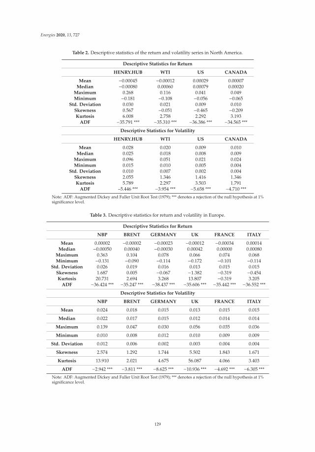
Energies 2020, 13, 727

Table 2. Descriptive statistics of the return and volatility series in North America.

Descriptive Statistics for Return

HENRY.HUB WTI US CANADA

Mean −0.00045 −0.00012 0.00029 0.00007Median −0.00080 0.00060 0.00079 0.00020

Maximum 0.268 0.116 0.041 0.049Minimum −0.181 −0.108 −0.056 −0.065

Std. Deviation 0.030 0.021 0.009 0.010Skewness 0.567 −0.051 −0.465 −0.209Kurtosis 6.008 2.758 2.292 3.193

ADF −35.791 *** −35.310 *** −36.386 *** −34.565 ***

Descriptive Statistics for Volatility

HENRY.HUB WTI US CANADA

Mean 0.028 0.020 0.009 0.010Median 0.025 0.018 0.008 0.009

Maximum 0.096 0.051 0.021 0.024Minimum 0.015 0.010 0.005 0.004

Std. Deviation 0.010 0.007 0.002 0.004Skewness 2.055 1.346 1.416 1.346Kurtosis 5.789 2.297 3.503 1.791

ADF –5.446 *** −3.954 *** −5.658 *** −4.710 ***

Note: ADF: Augmented Dickey and Fuller Unit Root Test (1979); *** denotes a rejection of the null hypothesis at 1%significance level.

Table 3. Descriptive statistics for return and volatility in Europe.

Descriptive Statistics for Return

NBP BRENT GERMANY UK FRANCE ITALY

Mean 0.00002 −0.00002 −0.00023 −0.00012 −0.00034 0.00014Median −0.00050 0.00040 −0.00030 0.00042 0.00000 0.00080

Maximum 0.363 0.104 0.078 0.066 0.074 0.068Minimum −0.131 −0.090 −0.114 −0.172 −0.101 −0.114

Std. Deviation 0.026 0.019 0.016 0.013 0.015 0.015Skewness 1.687 0.005 −0.067 −1.382 −0.319 −0.454Kurtosis 20.731 2.694 3.268 13.807 −0.319 3.205

ADF −36.424 *** −35.247 *** −38.437 *** −35.606 *** −35.442 *** −36.552 ***

Descriptive Statistics for Volatility

NBP BRENT GERMANY UK FRANCE ITALY

Mean 0.024 0.018 0.015 0.013 0.015 0.015

Median 0.022 0.017 0.015 0.012 0.014 0.014

Maximum 0.139 0.047 0.030 0.056 0.035 0.036

Minimum 0.010 0.008 0.012 0.010 0.009 0.009

Std. Deviation 0.012 0.006 0.002 0.003 0.004 0.004

Skewness 2.574 1.292 1.744 5.502 1.843 1.671

Kurtosis 13.910 2.021 4.675 56.087 4.066 3.403

ADF −2.942 *** −3.811 *** −8.625 *** −10.936 *** −4.692 *** −6.305 ***

Note: ADF: Augmented Dickey and Fuller Unit Root Test (1979); *** denotes a rejection of the null hypothesis at 1%significance level.

129

Energies 2020, 13, 727


5.1. Spillover Results

We followed Diebold and Yilmaz [1] (hence, DY12) to obtain the spillover effects in the timedomain. We first estimated the four variables in our VAR model in the North American market andthe six variables in our VAR model in the European market. Then, we used the generalized variancedecomposition for a forecast error to set up the spillover table to measure the direction and intensity ofspillover across the selected markets.

Next, in frequency domain, following Barunik and Krehlik [2] (hence, BK18), we used Fouriertransform to decompose the spillover table in the DY12 model into three different frequency bands,stated in Toyoshima and Hamori [20] as the short-term, “Fre S,” roughly corresponding to 1 to 5 days;the medium-term, “Fre M,” roughly corresponding to 6 to 21 days; and the long-term, “Fre L,” roughlycorresponding to 22 days to infinity.

In this study, the lag length of the VAR model is based on the AIC. According to our BK18 model,if the forecasting horizon is (H) < 100, the method is invalid. Consequently, we used a 100-day aheadforecasting horizon (H) for variance decomposition.

In Table 4, Table 5, we show the return spillover results from DY12 and BK18, which include thetwo markets: North America and Europe. Specifically, Tables 4 and 5 includes four sub-tables. At thetop are the results of the DY12, followed by the short-term, the medium-term, and the long-term resultsfrom the BK18. In each sub-table, the values in the ith row and the jth column equate to the strength ofthe spillover effect from the jth market to the ith market. For example, in the DY12 return spilloverresults in the North American market, the strength of the spillover effect in the third column (US) andthe second row (WTI) is 2.264. The values in the last row called “TO” indicate the mean value of thespillover effect on the other markets, whereas the values in the last column called “FROM” indicate themean value of the spillover effect from the other markets. The total spillover is the summary of all“TO” or “FROM” (for example, 17.165, as shown in the lower right corner).

Table 4. The return spillover table of DY, 2012 and BK, 2016 (North America).

North America (Return)

Spillover Results (DY12)

HENRY.HUB WTI US CANADA FROM

HENRY.HUB 98.033 1.425 0.147 0.394 0.492WTI 1.177 82.863 2.264 13.697 4.284US 0.163 2.242 79.294 18.301 5.177

CANADA 0.318 11.8 16.73 71.151 7.212TO 0.415 3.867 4.785 8.098 17.165

Spillover Results (BK18)

Frequency S 1–5 Days


HENRY.HUB 82.275 1.237 0.117 0.326 0.42WTI 0.968 68.456 1.825 10.802 3.399US 0.157 1.94 64.922 14.496 4.148

CANADA 0.227 9.137 12.591 55.607 5.489TO 0.338 3.078 3.633 6.406 13.455

Frequency M 6–21 Days


HENRY.HUB 11.643 0.14 0.022 0.05 0.053WTI 0.154 10.627 0.322 2.127 0.651US 0.005 0.223 10.591 2.796 0.756

CANADA 0.067 1.956 3.033 11.414 1.264TO 0.056 0.58 0.844 1.243 2.724

130

Energies 2020, 13, 727

Table 4. Cont.

Frequency L 22–Infinite Days


HENRY.HUB 4.116 0.049 0.008 0.018 0.019WTI 0.055 3.78 0.117 0.768 0.235US 0.002 0.079 3.781 1.009 0.272

CANADA 0.025 0.708 1.106 4.13 0.46TO 0.02 0.209 0.308 0.449 0.986

Note: Freq S: the spillover at “Freq S” roughly corresponds to 1 to 5 days; Freq M: the spillover at “Freq M” roughlycorresponds to 6 to 21 days; Freq L: the spillover at “Freq L” roughly corresponds to 22 to infinite days.

Table 5. Return spillover table of DY (2012) and BK (2018) (Europe).

Europe (Return)


NBP BRENT GERMANY UK FRANCE ITALY FROM

NBP 95.472 1.562 0.229 1.249 0.899 0.588 0.755BRENT 1.476 80.502 0.859 5.142 6.353 5.667 3.25

GERMANY 0.315 1.176 85.497 1.441 5.395 6.177 2.417UK 0.757 3.889 1.016 59.907 18.122 16.309 6.682

FRANCE 0.487 3.882 3.076 14.526 48.209 29.82 8.632ITALY 0.353 3.452 3.568 13.401 30.282 48.944 8.509

TO 0.565 2.327 1.458 5.96 10.175 9.76 30.245




NBP 77.614 1.2 0.177 0.926 0.656 0.456 0.569BRENT 1.364 66.891 0.795 4.062 5.013 4.614 2.641

GERMANY 0.31 0.797 71.894 1.123 4.185 4.976 1.898UK 0.624 2.975 0.799 48.48 14.355 13.195 5.325

FRANCE 0.452 2.943 2.373 11.673 38.348 23.9 6.89ITALY 0.332 2.792 2.84 11.254 24.717 40.276 6.989

TO 0.514 1.785 1.164 4.84 8.154 7.857 24.313



NBP 13.161 0.266 0.038 0.236 0.178 0.097 0.136BRENT 0.085 10.047 0.048 0.794 0.985 0.775 0.448

GERMANY 0.005 0.277 10.052 0.233 0.889 0.884 0.381UK 0.098 0.67 0.16 8.414 2.768 2.292 0.998

FRANCE 0.027 0.688 0.517 2.099 7.252 4.357 1.281ITALY 0.016 0.486 0.536 1.587 4.102 6.393 1.121

TO 0.038 0.398 0.216 0.825 1.487 1.401 4.365



NBP 4.697 0.097 0.014 0.087 0.065 0.035 0.05BRENT 0.028 3.564 0.016 0.286 0.355 0.278 0.16

GERMANY 0.001 0.101 3.551 0.084 0.322 0.317 0.137UK 0.035 0.243 0.058 3.013 0.999 0.822 0.359

FRANCE 0.008 0.25 0.187 0.753 2.61 1.564 0.46ITALY 0.005 0.174 0.192 0.56 1.463 2.275 0.399

TO 0.013 0.144 0.078 0.295 0.534 0.503 1.567


131

Energies 2020, 13, 727

Next, we identify some specifics when we compare the difference between the return spillovereffect in North America and in Europe using the pure time-domain approach of DY12. First, for thetotal return spillover effect, we can see that the total return spillover effect in Europe (30.245%) isstronger than that in North America (17.165%). This demonstrates that the return connectedness ofnatural gas, crude oil, and the electricity utility sector index in Europe is stronger than that in NorthAmerica. Whether in North America or Europe, the total return spillover of crude oil contributes morethan natural gas to the electricity utility stock market in each country. Further, in North America,Canada receives a greater effect from the two energy futures (0.318% from natural gas and 11.8% fromcrude oil) compared with the US in the time domain. In contrast, Canada exerts a greater effect on thenatural gas (0.394%) and crude oil (13.697%) sectors in the time domain. In Europe, the UK receivesthe greatest effect from the two energy futures (0.757% from natural gas and 3.889% from crude oil)compared with the other three countries in the time domain. The UK transmits the greatest effect onnatural gas (1.249%), but France transmits the greatest effect on crude oil (6.353%) in the time domain,which contrasts with the situation in North America. Finally, we find that there are some differences inthe return spillover effect among the two commodity markets and the stock market in North Americaand Europe, respectively. In North America, we find that the US receives a greater return spillovereffect on natural gas (0.163%) and transmits less of an effect (0.147%). In contrast to the US, Canadatransmits more of a return spillover effect on natural gas (0.394%) and receives a smaller effect (0.318%).In contrast to the natural gas market, the US transmits more of a return spillover effect on crude oil(2.264%) and receives a smaller effect (2.242%). In the same vein as the US, Canada also transmits moreof a return spillover effect on crude oil (13.697%) and receives a smaller effect (11.8%).

In Europe, except for Germany, the other three stock markets transmit more of a return spillovereffect on natural gas and receive a smaller effect. In the same vein as the situation for natural gas,except for Germany, the other three stock markets transmit more of a return spillover effect on crudeoil and receive a smaller effect. In terms of frequency, Tables 4 and 5 reveal that looking at either NorthAmerica or Europe, the total return spillover in the short-term (Frequency S 1–5 Days) is the highest,followed by the medium-term (Frequency M 6–21 Days) and the long-term (Frequency L 22–InfinityDays). These results suggest that the return shocks from any market transmitted to another marketwill not exceed one week.

Table 6, Table 7 show the volatility spillover results of DY12 and BK18 with the same construction.Table 6 shows the volatility spillover effect in North America, and Table 7 shows the effect in Europe.In time domain of DY12, we find the following. The total volatility spillover effect in Europe (27.929%)is stronger than that in in North America (20.216%). This situation is the same for the total returnspillover; whether in North America or Europe, the total volatility spillover of crude oil transmits morethan natural gas to the electricity utility stock market in each country. In North America, between thetwo stock markets, Canada receives the greatest spillover effect from natural gas (0.664%), and the USreceives the greatest effect from crude oil (6.771%) in the time domain. Among the two commoditymarkets, WTI is the most influential market on the stock market, transmitting the largest volatilityspillover to the US (6.771%) and Canada (6.302%) and is also the market that receives the largestvolatility spillover from the US (4.373%) and Canada (19.036%) compared with the natural gas market.

In the European market, among the four stock markets, the UK receives the largest effect fromnatural gas (0.785%), and Germany receives the largest effect from crude oil (4.56%) in the time domain.However, the UK transmits the largest effect on crude oil (8.843%), and Germany transmits the largesteffect on natural gas (2.374%) compared with other countries in the time domain. In addition, in termsof frequency and in contrast to the return spillover, Tables 6 and 7 reveal that in both North Americaand Europe, the total volatility spillover for the long-term (Frequency L 22–Infinity Days) is the highest,followed by the medium-term (Frequency M 6–21 Days) and the short-term (Frequency S 1–5 Days).These results imply that volatility shocks have a long-lasting effect.

132

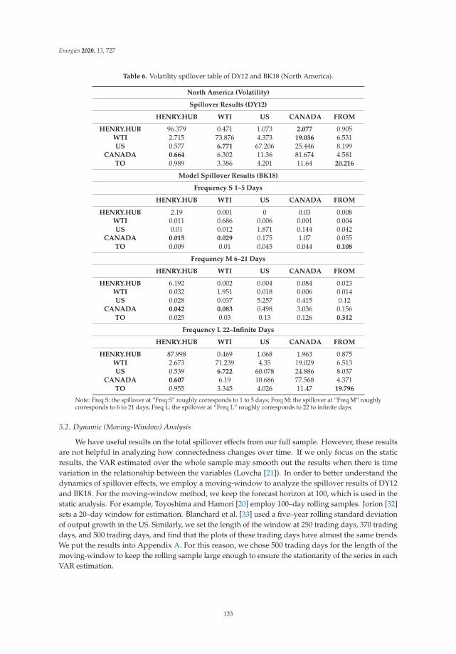
Energies 2020, 13, 727

Table 6. Volatility spillover table of DY12 and BK18 (North America).

North America (Volatility)



HENRY.HUB 96.379 0.471 1.073 2.077 0.905WTI 2.715 73.876 4.373 19.036 6.531US 0.577 6.771 67.206 25.446 8.199

CANADA 0.664 6.302 11.36 81.674 4.581TO 0.989 3.386 4.201 11.64 20.216

Model Spillover Results (BK18)



HENRY.HUB 2.19 0.001 0 0.03 0.008WTI 0.011 0.686 0.006 0.001 0.004US 0.01 0.012 1.871 0.144 0.042

CANADA 0.015 0.029 0.175 1.07 0.055TO 0.009 0.01 0.045 0.044 0.108



HENRY.HUB 6.192 0.002 0.004 0.084 0.023WTI 0.032 1.951 0.018 0.006 0.014US 0.028 0.037 5.257 0.415 0.12

CANADA 0.042 0.083 0.498 3.036 0.156TO 0.025 0.03 0.13 0.126 0.312



HENRY.HUB 87.998 0.469 1.068 1.963 0.875WTI 2.673 71.239 4.35 19.029 6.513US 0.539 6.722 60.078 24.886 8.037

CANADA 0.607 6.19 10.686 77.568 4.371TO 0.955 3.345 4.026 11.47 19.796


5.2. Dynamic (Moving-Window) Analysis

We have useful results on the total spillover effects from our full sample. However, these resultsare not helpful in analyzing how connectedness changes over time. If we only focus on the staticresults, the VAR estimated over the whole sample may smooth out the results when there is timevariation in the relationship between the variables (Lovcha [21]). In order to better understand thedynamics of spillover effects, we employ a moving-window to analyze the spillover results of DY12and BK18. For the moving-window method, we keep the forecast horizon at 100, which is used in thestatic analysis. For example, Toyoshima and Hamori [20] employ 100–day rolling samples. Jorion [32]sets a 20–day window for estimation. Blanchard et al. [33] used a five–year rolling standard deviationof output growth in the US. Similarly, we set the length of the window at 250 trading days, 370 tradingdays, and 500 trading days, and find that the plots of these trading days have almost the same trends.We put the results into Appendix A. For this reason, we chose 500 trading days for the length of themoving-window to keep the rolling sample large enough to ensure the stationarity of the series in eachVAR estimation.

133

Energies 2020, 13, 727

Table 7. Volatility spillover table of) DY12 and BK18 (Europe).

Europe (Volatility)



NBP 95.825 0.142 2.374 0.57 0.315 0.775 0.696BRENT 7.628 72.585 0.516 8.843 3.489 6.939 4.569

GERMANY 0.372 4.56 85.188 0.815 4.103 4.962 2.469UK 0.785 4.186 0.68 69.947 11.411 12.99 5.009

FRANCE 0.061 1.067 2.13 10.504 56.435 29.804 7.261ITALY 0.252 0.382 2.676 9.658 34.583 52.448 7.925

TO 1.517 1.723 1.396 5.065 8.984 9.245 27.929




NBP 4.619 0.003 0.001 0.001 0.001 0.002 0.001BRENT 0.012 0.645 0 0.004 0.008 0.001 0.004

GERMANY 0.002 0.002 5.888 0.001 0.03 0.026 0.01UK 0.003 0.013 0.003 7.448 0.889 0.892 0.3

FRANCE 0 0.02 0.004 0.101 0.9 0.34 0.078ITALY 0.002 0.037 0.009 0.217 0.642 1.782 0.151

TO 0.003 0.012 0.003 0.054 0.262 0.21 0.544



NBP 12.611 0.007 0.036 0.016 0.008 0.014 0.013BRENT 0.042 1.839 0.002 0.042 0.033 0.027 0.024

GERMANY 0.021 0.017 15.534 0.025 0.072 0.063 0.033UK 0.011 0.052 0.027 17.694 2.135 2.188 0.735

FRANCE 0.002 0.056 0.017 0.33 2.589 1.011 0.236ITALY 0.005 0.099 0.043 0.677 1.849 4.933 0.446

TO 0.013 0.038 0.021 0.181 0.683 0.551 1.487



NBP 78.595 0.133 2.337 0.553 0.306 0.758 0.681BRENT 7.574 70.100 0.514 8.798 3.448 6.910 4.541

GERMANY 0.350 4.541 63.766 0.789 4.000 4.873 2.426UK 0.772 4.121 0.650 44.805 8.387 9.910 3.973

FRANCE 0.059 0.991 2.109 10.073 52.945 28.453 6.947ITALY 0.245 0.246 2.624 8.764 32.092 45.733 7.329

TO 1.500 1.672 1.372 4.829 8.039 8.484 25.898


As displayed in Figure 4a,b, we find some characteristics from the dynamics of the total returnspillover and the frequency decomposition of North America and Europe. In both North America andEurope, the total return spillover occurs in the short-term. Moreover, two dynamic return spilloverfigures have a similar trend. In Europe, the total spillover of the DY12 model for the return series variesbetween 20% and 45%, which is wider than that in North America (between 10% and 30%). From 2009to mid–2013, whether in North America or Europe, the total return spillover retains high stability,which may be a consequence of the effect of the 2008 global financial crisis or the 2010 Europeansovereign debt crisis. The total return spillover in both North America and Europe began to increasesteadily until around 2017, which could be influenced by the 2014 international crude oil crisis.

134

Energies 2020, 13, 727

(a)

(b)

Figure 4. (a) The total return spillover of DY12 andBK18 in North America (Windows 500). (b) Thetotal return spillover of DY12 and BK18 in Europe (Windows 500). Note: The yellow line indicates thetotal spillover index of the DY12 model; the red line indicates the total spillover index at “Freq S” of theBK18 model; the green line indicates the total spillover index at “Freq M” of the BK18 model; the blueline indicates the total spillover index at “Freq L” of the BK18 model. The vertical axis variable unit isin percentages.

As seen in Figure 5a,b, which shows the dynamics of total volatility spillover and frequencydecomposition for North America and Europe, the total spillover fluctuates more than the total returnspillover. Moreover, the total volatility spillover reacts more violently to extreme events than that ofthe returns. In contrast with the total return spillover, the total volatility spillover develops over thelong-term. This means that the total volatility spillover is more sensitive to shocks and extreme events;unlike the total return spillover, whether in North America or Europe, the total volatility spillover ofDY12 shifts between 0% and 60%. From 2009 to mid-2013, whether in North America or Europe, thetotal volatility spillover retained its stability, which may be a consequence of the 2008 global financialcrisis and the 2009 European sovereign debt crisis. In North America, we identified some suddenfluctuations, such as a sharp increase in 2015 and 2016, an increasing trend from 2017 to 2018, anda sudden rise in 2019. These fluctuations may have been influenced by the 2014 international crude

135

Energies 2020, 13, 727

oil crisis, the 2016 Organization of the Petroleum Exporting Countries announcement to cut suppliesat the end of 2017, the 2017 summer Hurricane Irma, and the 2019 trade war between China and theUS. However, in Europe, we see almost the same fluctuations from mid-2013 to 2016; around 2015to mid-2016, there are two sudden fluctuations that may be a result of some extreme events, such asthe 2014 international crude oil crisis and the 2016 Brexit event. We also investigated the dynamics ofthe total return and volatility spillover in different windows and the pairwise directional return andvolatility spillover in two regions. The results are given in Appendix A.

(a)

(b)

Figure 5. (a) The total volatility spillover of DY12 and BK18 in North America (Windows 500). (b) Thetotal volatility spillover of DY12 and BK18 in Europe (Windows 500). Note: The yellow line indicatesthe total spillover index of the DY12 model; the red line indicates the total spillover index at “Freq S” ofthe BK18 model; the green line indicates the total spillover index at “Freq M” of the BK18 model; theblue line indicates the total spillover index at “Freq L” of the BK18 model. The vertical axis variableunit is in percentages.

136

Energies 2020, 13, 727

6. Concluding Remarks

Our paper discusses the return and volatility spillover across the natural gas market, crude oilmarket, and stock market from 4 August 2009 to 16 August 2019 to assess the information transmissionand risk transmission among the three markets by employing a new method for time–frequencydeveloped by Diebold and Yilmaz [1] and Barunik and Krehlik [2]. It is crucial to investigate thespillover effects not only for investors to adjust their investment programs but also for governmentauthorities to make proper economic decisions. The contributions of our paper to the literature areas follows.

First, in time domain, the total return and volatility spillover in Europe are stronger than in NorthAmerica. Moreover, whether in North America or in Europe, the spillover table reveals that crude oil,rather than natural gas, has the greatest effect on electricity utility stock markets. In North America,Canada not only receives a larger return spillover effect from the two energy futures (0.318% fromnatural gas, 11.8% from crude oil) compared with the US but also transmits a greater effect on the twoenergy futures. Regarding volatility spillover, Canada still has the largest spillover effect on the othertwo energy futures and receives the largest volatility effect from natural gas. However, the US receivesthe largest volatility spillover effect from crude oil (6.771%). In Europe, the UK receives the greatestreturn spillover effect from the two energy futures (0.757% from natural gas and 3.889% from crude oil)compared with the other three countries. The UK transmits the largest effect on natural gas (1.249%),but France transmits the largest effect on crude oil (6.353%) in the time domain, which is different thanthe situation in North America. Regarding volatility spillover, the UK receives the largest effect fromnatural gas (0.785%), and Germany receives the largest from crude oil (4.56%). However, FTSE350(the UK) transmits the largest effect on crude oil (8.843%), and Germany transmits the largest effect onnatural gas (2.374%) compared to the other countries.

Second, in terms of frequency, our results show that the short-term has the largest effect on returnspillover; however, the long-term has the largest effect on volatility spillover in both North Americaand Europe. These results imply that the return shocks from any market transmitted to another marketwill not exceed one week, whereas the results of volatility spillovers imply that volatility shocks havea long-lasting effect. This conclusion is consistent with the results of Barunik and Krehlik [2] andTiwari et al. [34].

Third, in terms of return spillover transmission, all markets respond to return shocks immediately.The total return spillover effect in the short-term was the greatest. In this case, it is difficult to determinethe impact of a particular market on another market. Unlike return spillover transmissions, the totalvolatility spillover effect in the long-term was the greatest. Policymakers have sufficient time to preventthe impact of extreme volatility shocks on other markets. In addition, based on a summary of theresults above, the volatility of natural gas is less than that of oil, which suggests that compared withoil, natural gas investors may have a greater opportunity to make a profit.

Forth, some interesting results are displayed in the rolling analyses. For example, because of thesubsequent effect of the 2008 global financial crisis and the 2010 European sovereign debt crisis, thereturn and volatility spillover in both North America and Europe maintained a high level. Due tothe later 2014 international oil crisis, both North America and Europe fluctuated fiercely around 2015.Around mid-2016, the Brexit event made the volatility spillover in Europe increase suddenly.

Author Contributions: Conceptualization, T.N. and S.H.; investigation, W.Z. and X.H.; writing—original draftpreparation, W.Z.; writing—review and editing, X.H., T.N., and S.H.; project administration, S.H.; fundingacquisition, S.H. All authors have read and agreed to the published version of the manuscript.


Acknowledgments: We are grateful to Mehmet H. Bilgin and four anonymous referees for helpful commentsand suggestions.


137

Energies 2020, 13, 727

Appendix A

Figure A1. Pairwise directional return spillover of DY12 and BK18 in North America. Notes: US fromHENRY HUB indicates the return spillover from natural gas to US; CANADA from HENRY HUBindicates the return spillover from natural gas to Canada; US from WTI indicates the return spilloverfrom crude oil to US; CANADA from WTI indicates the return spillover from crude oil to Canada.

Figure A2. Pairwise directional return spillover of DY12 and BK18 in Europe. Notes: GERMANY fromNBP indicates the return spillover from natural gas to Germany; UK from NBP indicates the returnspillover from natural gas to the UK; FRANCE from NBP indicates the return spillover from naturalgas to France; ITALY from NBP indicates the return spillover from natural gas to Italy; GERMANYfrom BRENT indicates the return spillover from crude oil to Germany; UK from BRENT indicates thereturn spillover from crude oil to the UK; FRANCE from BRENT indicates the return spillover fromcrude oil to France; ITALY from BRENT indicates the return spillover from crude oil to Italy.

138

Energies 2020, 13, 727

Figure A3. Pairwise directional volatility spillover of DY12 and BK18 in North America. Notes: USfrom HENRY HUB indicates the volatility spillover from natural gas to US; CANADA from HENRYHUB indicates the volatility spillover from natural gas to Canada; US from WTI indicates the volatilityspillover from crude oil to US; CANADA from WTI indicates the volatility spillover from crude oilto Canada.

Figure A4. Pairwise directional volatility spillover of DY12 and BK18 in Europe. Notes: GERMANYfrom NBP indicates the volatility spillover from natural gas to Germany; UK from NBP indicates thevolatility spillover from natural gas to the UK; FRANCE from NBP indicates the volatility spilloverfrom natural gas to France; ITALY from NBP indicates the volatility spillover from natural gas to Italy;GERMANY from BRENT indicates the volatility spillover from crude oil to Germany; UK from BRENTindicates the volatility spillover from crude oil to the UK; FRANCE from BRENT indicates the volatilityspillover from crude oil to France; ITALY from BRENT indicates the volatility spillover from crude oilto Italy.

139

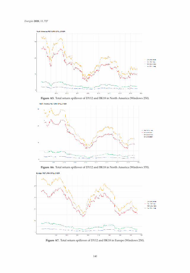
Energies 2020, 13, 727

Figure A5. Total return spillover of DY12 and BK18 in North America (Windows 250).

Figure A6. Total return spillover of DY12 and BK18 in North America (Windows 370).

Figure A7. Total return spillover of DY12 and BK18 in Europe (Windows 250).

140

Energies 2020, 13, 727

Figure A8. Total return spillover of DY12 and BK18 in Europe (Windows 370).

Figure A9. Total volatility spillover of DY12 and BK18 in North America (Windows 250).

Figure A10. Total volatility spillover of DY12 and BK18 in North America (Windows 370).

141

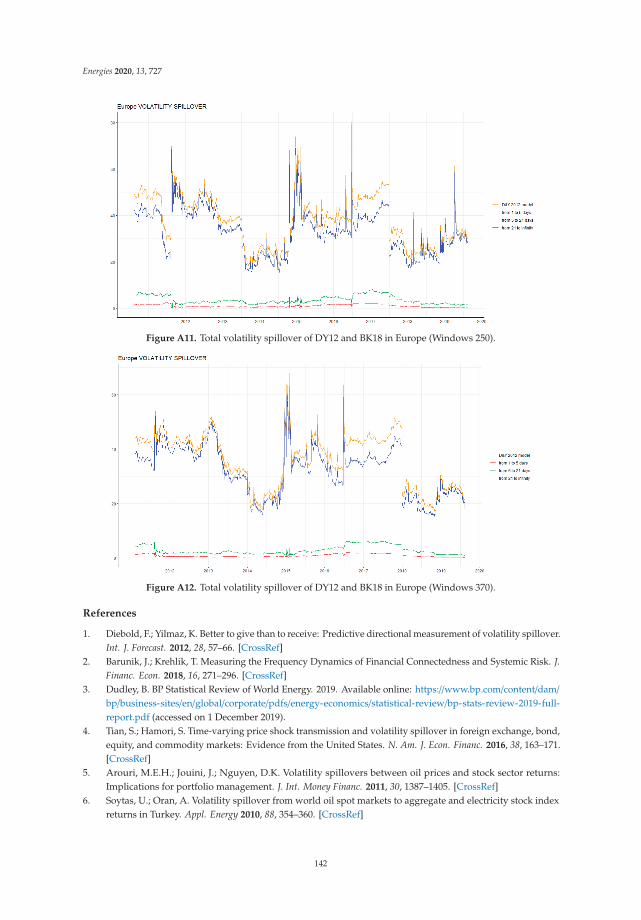
Energies 2020, 13, 727

Figure A11. Total volatility spillover of DY12 and BK18 in Europe (Windows 250).

Figure A12. Total volatility spillover of DY12 and BK18 in Europe (Windows 370).

References

1. Diebold, F.; Yilmaz, K. Better to give than to receive: Predictive directional measurement of volatility spillover.Int. J. Forecast. 2012, 28, 57–66. [CrossRef]

2. Barunik, J.; Krehlik, T. Measuring the Frequency Dynamics of Financial Connectedness and Systemic Risk. J.Financ. Econ. 2018, 16, 271–296. [CrossRef]

3. Dudley, B. BP Statistical Review of World Energy. 2019. Available online: https://www.bp.com/content/dam/bp/business-sites/en/global/corporate/pdfs/energy-economics/statistical-review/bp-stats-review-2019-full-report.pdf (accessed on 1 December 2019).

4. Tian, S.; Hamori, S. Time-varying price shock transmission and volatility spillover in foreign exchange, bond,equity, and commodity markets: Evidence from the United States. N. Am. J. Econ. Financ. 2016, 38, 163–171.[CrossRef]

5. Arouri, M.E.H.; Jouini, J.; Nguyen, D.K. Volatility spillovers between oil prices and stock sector returns:Implications for portfolio management. J. Int. Money Financ. 2011, 30, 1387–1405. [CrossRef]

6. Soytas, U.; Oran, A. Volatility spillover from world oil spot markets to aggregate and electricity stock indexreturns in Turkey. Appl. Energy 2010, 88, 354–360. [CrossRef]

142

Energies 2020, 13, 727

7. Cheung, Y.; Ng, L.K. A causality-in-variance test and its application to financial market prices. J. Econom.1996, 72, 33–48. [CrossRef]

8. Arouri, M.E.H.; Lahiani, A.; Nguyen, D.K. Return and volatility transmission between world oil prices andstock markets of the GCC countries. Econ. Model. 2011, 28, 1815–1825. [CrossRef]

9. Nazlioglus, S.; Erdem, C.; Soytas, U. Volatility spillover between oil and agricultural commodity markets.Energy Econ. 2012, 36, 658–665. [CrossRef]

10. Nakajima, T.; Hamori, S. Causality-in-Mean and Causality-in-Variance among Electricity Prices, Crude OilPrices, and Yen-US Dollar Exchange Rates in Japan. Res. Int. Bus. Financ. 2012, 26, 371–386. [CrossRef]

11. Ewing, B.T.; Malik, F.; Ozfidan, O. Volatility transmission in the oil and natural gas markets. Energy Econ.2002, 24, 525–538. [CrossRef]

12. Acaravci, A.; Ozturk, I.; Kandir, S.Y. Natural gas prices and stock prices: Evidence from EU-15 countries.Econ. Model. 2012, 29, 1646–1654. [CrossRef]

13. Johansen, S.; Juselius, K. Maximum likelihood estimation and inference on cointegration—With applicationsto the demand for money. Oxf. Bull. Econ. Stat. 1990, 52, 169–210. [CrossRef]

14. Diebold, F.X.; Yilmaz, K. On the network topology of variance decompositions: Measuring the connectednessof financial firms. J. Econ. 2014, 182, 119–134. [CrossRef]

15. Diebold, F.X.; Yilmaz, K. Financial and Macroeconomic Connectedness: A Network Approach to Measurement andMonitoring, 1st ed.; Oxford University Press: Oxford, UK, 2015.

16. Maghyereh, A.I.; Awartani, B.; Bouri, E. The directional volatility connectedness between crude oil andequity markets: New evidence from implied volatility indexes. Energy Econ. 2016, 57, 78–93. [CrossRef]

17. Duncan, A.S.; Kabundi, A. Domestic and foreign sources of volatility spillover to South African asset classes.Econ. Model. 2013, 31, 566–573. [CrossRef]

18. Liow, K.H. Volatility spillover dynamics and relationship across G7 financial markets. N. Am. J. Econ. Financ.2015, 33, 328–365. [CrossRef]

19. Sugimoto, K.; Matsuki, T.; Yoshida, Y. The global financial crisis: An analysis of the spillover effects onAfrican stock markets. Emerg. Mark. Rev. 2014, 21, 201–233. [CrossRef]

20. Toyoshima, Y.; Hamori, S. Measuring the Time-Frequency Dynamics of Return and Volatility Connectednessin Global Crude Oil Markets. Energies 2018, 11, 2893. [CrossRef]

21. Lovcha, Y.; Perez-Laborda, A. Dynamic frequency connectedness between oil and natural gas volatilities.Econ. Model. 2020, 84, 181–189. [CrossRef]

22. Ferrer, R.; Shahzad, S.J.H.; Lopez, R.; Jareno, F. Time and frequency dynamics of connectedness betweenrenewable energy stocks and crude oil prices. Energy Econ. 2018, 76, 1–20. [CrossRef]

23. Zhang, B.; Wang, P. Return and volatility spillovers between china and world oil markets. Econ. Model. 2014,42, 413–420. [CrossRef]

24. Oberndorfer, U. Energy prices, volatility, and the stock market: Evidence from the Eurozone. Energy Policy2009, 37, 5787–5795. [CrossRef]

25. Kenourgios, D.; Christopoulos, A.G.; Dimitriou, D. Asset Markets Contagion during the Global FinancialCrisis. Multinatl. Financ. J. 2013, 17, 49–76. [CrossRef]

26. Kenourgios, D.; Dimitriou, D. Contagion of the Global Financial Crisis and the real economy: A regionalanalysis. Econ. Model. 2015, 44, 283–293. [CrossRef]

27. Baur, D.G. Financial contagion and the real economy. J. Bank. Financ. 2012, 36, 2680–2692. [CrossRef]28. Singh, P.; Kumar, B.; Pandey, A. Price and volatility spillovers across North American, European and Asian

stock markets. Int. Rev. Financ. Anal. 2010, 19, 55–64. [CrossRef]29. Balli, F.; Hajhoj, H.R.; Basher, S.A.; Ghassan, H.B. An analysis of returns and volatility spillovers and their

determinants in emerging Asian and Middle Eastern countries. Int. Rev. Econ. Financ. 2015, 39, 311–325.[CrossRef]

30. Koop, G.; Pesaran, M.H.; Potter, S.M. Impulse response analysis in nonlinear multivariate models. J. Econ.1996, 74, 119–147. [CrossRef]

31. Pesaran, H.H.; Shin, Y. Generalized Impulse Response Analysis in Linear Multivariate Models. Econ. Lett.1998, 58, 17–29. [CrossRef]

32. Jorion, P. Predicting volatility in the foreign exchange market. J. Financ. 1995, 50, 507–528. [CrossRef]

143

Energies 2020, 13, 727

33. Blanchard, O.; Simon, J. The long and large decline in U.S. output volatility. Brook. Pap. Econ. Act. 2001, 32,135–174. [CrossRef]

34. Tiwari, A.K.; Cunado, J.; Gupta, R.; Wohar, M.E. Volatility spillovers across global asset classes: Evidencefrom time and frequency domains. Q. Rev. Econ. Financ. 2018, 70, 194–202. [CrossRef]


144

energies

Article

Connectedness Between Natural Gas Price and BRICSExchange Rates: Evidence from Time andFrequency Domains

Yijin He 1, Tadahiro Nakajima 1,2 and Shigeyuki Hamori 1,*

1 Graduate School of Economics, Kobe University, 2-1, Rokkodai, Nada-Ku, Kobe 657-8501, Japan;[email protected] (Y.H.); [email protected] (T.N.)

2 The Kansai Electric Power Company, Incorporated, 6-16, Nakanoshima 3-chome,Kita-Ku, Osaka 530-8270, Japan

* Correspondence: [email protected]

Received: 27 August 2019; Accepted: 16 October 2019; Published: 18 October 2019

Abstract: In this paper, we investigate the connectedness between natural gas and BRICS (Brazil,Russia, India, China, and South Africa)’s exchange rate in terms of time and frequency. This empiricalwork is based on the approach of connectedness proposed by Diebold and Yilmaz, who providedan effective way of valuing how much variation in one variable is responsible for the value of othervariables, and the method proposed by Baruník and Krehlík, who decomposed the results fromDiebold and Yilmaz into different frequencies. We also use the rolling-window method to conducttime-varying analysis. The data used in this paper are from 23 August 2010 to 20 June 2019. We findthat the natural gas price hardly influences BRICS’s exchange rates, which provides an importantpractical implication for policymakers, especially in oil-dependent countries.

Keywords: BRICS; exchange rates; connectedness; time domain; frequency domain

1. Introduction

In light of the increasing attention being paid to environmental sustainability, energysystems are gradually transitioning from a dependence on non-renewable resources to the useof environment-friendly resources. This will have a great impact on day-to-day life, economies,businesses, manufacturers, and governments. Compared to coal or petroleum, natural gas has manyqualities that makes it burn more efficiently. It also generates fewer emissions of most types of airpollutants, including carbon dioxide. With the expansion of gas pipelines, the increasing number of gasliquefaction plants, and the exploitation of natural gas fields, it is reasonable to consider that the naturalgas trade will become more globalized. Natural gas has become a major part of the world’s energyconsumption, demand, and supply in recent years. In 2018, for example, natural gas consumption roseby 5.3%, one of the fastest rates of growth since 1984. With the continuing rapid expansion in liquefiednatural gas (LNG), the inter-regional natural gas trade grew by 4.3%, which was more than double the10-year average [1]. As reported in the Global Energy Perspective 2019: Reference Case [2], natural gaswill be the only fossil fuel whose share of total energy demand continues to increase until 2035, andChina will represent nearly half of the global demand growth. Other developing countries are alsoexpected to increase their demand for natural gas.

Brazil, Russia, India, China, and South Africa (BRICS), a group of five fast-growing developingcountries, play an important and expanding role in the world economy. In recent years, BRICS haverepresented an increasing share of global economic growth. According to the International MonetaryFund (IMF), as of 2018, the combined gross domestic product (GDP) of these five nations accountedfor 23.2% of the gross world product (GWP). Given the growth of BRICS and the fact that energy is


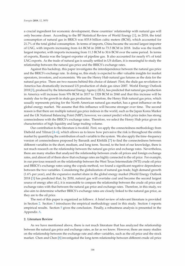
Energies 2019, 12, 3970

a crucial ingredient for economic development, these countries’ relationship with natural gas willonly become closer. According to the BP Statistical Review of World Energy [1], in 2018, the totalconsumption of natural gas in BRICS was 835.8 billion cubic meters (BCM), which accounted for21.7% of the total global consumption. In terms of imports, China became the second largest importerof LNG, with imports increasing from 4.6 BCM in 2008 to 73.5 BCM in 2018. India was the fourthlargest importer, with imports increasing from 11.3 BCM to 30.6 BCM over the same period. In termsof exports, Russia was the largest exporter of pipeline gas. It also accounted for nearly 6% of totalLNG exports. As the trade of natural gas is usually settled in US dollars, it is meaningful to study therelationship between the natural gas price and the BRICS’s exchange rates.

Against this backdrop, this paper investigates the interdependence between the natural gas priceand the BRICS’s exchange rate. In doing so, this study is expected to offer valuable insights for marketoperators, investors, and economists. We use the Henry Hub natural gas futures as the data for thenatural gas price. There are two reasons behind this choice of dataset: First, the shale gas revolution inAmerica has dramatically increased US production of shale gas since 2007. World Energy Outlook2018 [3], produced by the International Energy Agency (IEA), has predicted that natural gas productionin America will increase from 976 BCM in 2017 to 1328 BCM in 2040 and that this increase will bemainly due to the growth in shale gas production. Therefore, the Henry Hub natural gas price, whichusually represents pricing for the North American natural gas market, has a great influence on theglobal energy market. We assume that this influence will become stronger over time. The secondreason is that there are multiple natural gas price indexes in the world, such as the Japan Korea Markerand the UK National Balancing Point (NBP); however, we cannot predict which price index has strongconnectedness with the BRICS’s exchange rates. Therefore, we select the Henry Hub price given itscharacteristics of high liquidity and large trading volume.

Our contribution to the literature is twofold. First, we apply the connectedness methodology fromDiebold and Yilmaz [4–6], which allows us to know how pervasive the risk is throughout the entiremarket by quantifying the contribution of each variable to the system. We also apply the time–frequencyversion of connectedness proposed by Baruník and Krehlík [7] to find the connectedness betweendifferent variables in the short, medium, and long term. Second, to the best of our knowledge, there isnot much research on the relationship between the natural gas price and exchange rates. Nevertheless,there are many studies that analyzed the relationship between crude oil prices and foreign exchangerates, and almost all of them show that exchange rates are highly connected to the oil price. For example,in our previous research on the relationship between the West Texas Intermediate (WTI) crude oil priceand BRICS’s exchange rates using the copula method, we found a significant negative dependencebetween the two variables. Considering the globalization of natural gas trade, high demand growth(1.6% per year), and the expansive market share in the global energy market (World Energy Outlook2018 [3] has predicted that, by 2030, natural gas will overtake coal and become the second largestsource of energy after oil.), it is reasonable to compare the relationship between the crude oil price andexchange rates with that between the natural gas price and exchange rates. Therefore, in this study, wealso aim to determine whether BRICS’s exchange rates are closely linked to the natural gas price, asthey are to the oil price.

The rest of this paper is organized as follows: A brief review of relevant literature is providedin Section 2. Section 3 introduces the empirical methodology used in this study. Section 4 reportsempirical results. Section 5 gives the conclusion. Finally, a robustness analysis is presented in theAppendix A.


As we have mentioned above, there is not much literature that has analyzed the relationshipbetween the natural gas price and exchange rates, as far as we know. However, there are many studieson the relationship between the exchange rate and other variables, such as the oil price and the stockmarket. Chen and Chen [8] investigated the long-term relationship between different crude oil price

146

Energies 2019, 12, 3970

indexes and G7 countries’ exchange rates using the monthly panel data between January 1972 andDecember 2005. They found that oil prices may account for the movements of the real exchangerate and there is a link between oil prices and real exchange rates. Additionally, from the results ofpanel predictive regression, they found that the crude oil price has the ability to forecast the futureexchange rate. Andries, et al. [9] identified the patterns of co-movement of the interest rate, stockprice, and exchange rate in India using wavelet analysis. They used the data span from July 1997 toDecember 2010. The empirical results showed that exchange rates, interest rates, and stock pricesare linked to each other and that the stock price fluctuations lag behind both the exchange rates andinterest rates. Brahm et al. [10] used monthly data to investigate the relationship between the crude oilprice and exchange rates in the long term and short term, respectively. The data span was from January1997 to December 2009. Empirical results indicated exchange rates Granger-caused crude oil pricesin the short term, whereas crude oil Granger-caused exchange rates in the long term. Furthermore,based on impulse response analysis, exchange rate shock had a significant negative effect on crude oilprices. Jain and Pratap [11] explored the relationship between global prices of crude oil and gold, thestock market in India, and the USD–INR exchange rate using the DCC-GARCH (dynamic conditionalcorrelation-generalized autoregressive conditional heteroscedasticity) model. They also examined thelead lag linkages among these variables using symmetric and asymmetric non-linear causality tests.They used daily data from the period of 2006 to 2016, finding that a fall in the value of the IndianRupee and the benchmark stock index was caused by a fall in gold and crude oil prices.

On the empirical side, the methodology used in this paper has already been applied in manyfields. Maghyereh et al. [12] used implied volatility indices (VIX) of the daily close price of crudeoil in 11 countries. They found that the connectedness between oil and equity was dominated bythe transmissions from the oil market to equity markets and most of the linkages between these twomarkets were established from mid-2009 to mid-2012, a period that witnessed the start of the globalrecovery. Lundgren et al. [13] studied the renewable energy stock returns and their relation to theuncertainty of currency, oil price, stocks, and US treasury bonds. They used data covering the periodfrom 2004 to 2016, and found that the European stock market depends on renewable energy stockprices. Singh et al. [14] employed a dynamic and directional network connectedness between theimplied volatility index (VIX) of the exchange rates of nine major currency pairs and the crude oilusing the data between May 2017 and December 2017. They found that crude oil affected currenciesmore than currencies affected crude oil, but the reverse was true during the crude oil crisis period.Furthermore, their results revealed that EUR–USD is more sensitive to crude oil price fluctuation thanothers. Ji et al. [15] combined empirical mode decomposition with a connectedness methodology, andexamined the dynamic connectedness among crude oil, natural gas, and refinery products using dailydata between 3 January 2000 and 15 September 2017. Employing a constant analysis, they found thatcrude oil and its refinery product tend to be a net transmitter, while the natural gas tends to be anet receiver. In time-varying analysis, they found that the total connectedness generally increaseduntil the 2014 crude oil crash, and then decreased sharply. Lovch and Perez-Laborda [16] used theconnectedness method and frequency decomposition method to investigate the relationship betweenthe natural gas and crude oil price during the period from 1994 to 2018. They found that the volatilityconnectedness varied over time; the connectedness became weak after the financial crisis; and thevolatility had long-run effects, except during some specific periods, when volatility shocks transmittedfaster but dissipated in the short-run.

3. Empirical Methodology

In this paper, we employ two methods to establish the nature of the relationship between exchangerates and natural gas price. The first method is provided by Diebold and Yilmaz (DY) [4–6], whoseapproach calculates the connectedness between different objects by introducing variance decompositioninto vector autoregression (VAR) models. The second method is based on Baruník and Krehlík (BK) [7],who proposed a new framework to estimate connectedness by using a spectral representation of

147

Energies 2019, 12, 3970

variance decomposition. In conclusion, the DY framework describes the connectedness as “whenshocks are arising in one variable, how would other variables be changing?”, whereas the BK frameworkestimates the connectedness in short-, medium-, and long-term financial cycles.

3.1. Connectedness Table

Based on Diebold and Yilmaz [6], a simplified connectedness table is presented in Table 1, whichgives a clear picture of aggregated and disaggregated connectedness.

Table 1. Connectedness table.

x1 x2 . . . xN From

x1 d11 d12 . . . d1N∑N

j=1 d1 j j � 1

x2 d21 d22 . . . d2N∑N

j=1 d2 j j � 2

......

... . . . ......

xN dN1 dN2 . . . dNN∑N

j=1 dN j j � N

To∑N

i=1 di1i � 1

∑Ni=1 di2

i � 2. . .

∑Ni=1 diNi � N

1N

∑Ni, j=1 dij i �

j

Source: Diebold and Yilmaz (2015).

In the table, xi is the interested variable, whereas dij is the pairwise directional connectedness fromxj to xi, which shows what percentage of the h-step-ahead forecast error variance in xi is due to theshocks in xj (Equation (1)). We can simply understand dij as how much future uncertainty of xi is dueto the shocks in xj:

Ci← j = dij. (1)

The column “From” is the total directional connectedness from xj to others (Equation (2)), and therow “To” means the total directional connectedness from others to xi (Equation (3)):

C·← j =N∑

i = 1i � j

dij, (2)

Ci←· =N∑

j = 1j � i

dij. (3)

We were also interested in net pairwise directional connectedness (Equation (4)) and net totaldirectional connectedness (Equation (5)), which are expressed as a negative value to indicate a netrecipient and a positive value to indicate a net transmitter:

Cij = Cj←i −Ci← j, (4)

Ci = C·←i −Ci←· (5)

148

Energies 2019, 12, 3970

Finally, the total connectedness (Equation (6)), calculated by the grand total of the off-diagonalentries of dij, is given in the lower-right cell of the connectedness table:

C =1N

N∑i, j = 1

i � j

dij. (6)

3.2. Generalized Forecast Error Variance Decomposition (GFEVD)

Diebold and Yilmaz [4] measured connectedness based on forecast error variance decompositionsfrom VAR models, which were introduced by Sims [17] and Koop et al. [18]. However, the calculationof variance decomposition requires orthogonalized shocks and depends on ordering the variables, soDiebold and Yilmaz [5] exploited the generalized forecast error variance decomposition (GFEVD) ofPesaran and Shin [19] to solve those problems. In this paper, we employ the method of GFEVD tocalculate the connectedness.

We will give a brief introduction to GFEVD, followed by an explanation of Lütkepohl [20] andDiebold and Yilmaz [6].

For easy understanding, we first consider a VAR (1) process with N-variable:

yt = v + A1yt−1 + ut, t = 0,±1,±2 . . .E(ut) = 0

E(utu′t) = Σu

E(utu′s) = 0, t � s.

(7)

If the generation mechanism starts at time t = 1, we get:

y1 = v + A1y0 + u1

y2 = v + A1y1 + u2 = v + A1(v + A1y0 + u1) + u2

= (IN + A1)v + A21y0 + A1u1 + u2

. . .

yt = (IN + A1 + · · ·+ At−11 )v + At

1y0 +∑t−1

m=0 Am1 ut−m. . . . .

(8)

If all eigenvalues of A1 have modulus less than 1 (VAR process is stable), we have:

(IN + A1 + · · ·+ At−11 )v → (IN −A1)

−1v as t →∞At

1y0 → 0 as t →∞..(9)

Then, we can rewrite Equation (7) as:

yt = μ+∑∞

m=0 Am1 ut−m, t = 0,±1,±2 . . .

where μ ≡ (IN −A1)−1v.

(10)

Secondly, let us consider a VAR (p) process:

yt = v + A1yt−1 + · · ·+ Apyt−p + ut, t = 0,±1,±2, . . . (11)

149

Energies 2019, 12, 3970

By using matrices, we can rewrite the VAR (p) process as a VAR (1) process:

Yt = v + AYt−1 + Ut

Yt

(Np ∗ 1)≡

⎡⎢⎢⎢⎢⎢⎢⎢⎢⎢⎢⎢⎢⎣y1

y2

. . .yt−p+1

⎤⎥⎥⎥⎥⎥⎥⎥⎥⎥⎥⎥⎥⎦,v

(Np× 1)≡

⎡⎢⎢⎢⎢⎢⎢⎢⎢⎢⎢⎢⎢⎣v0. . .0

⎤⎥⎥⎥⎥⎥⎥⎥⎥⎥⎥⎥⎥⎦A

(Np×Np)≡

⎡⎢⎢⎢⎢⎢⎢⎢⎢⎢⎢⎢⎢⎢⎢⎢⎢⎢⎣A1

IN

0

A2

0IN

. . . Ap−1 Ap

. . . 0 0

. . . 0 0. . . . . . . . . . . . 00 0 . . . IN 0

⎤⎥⎥⎥⎥⎥⎥⎥⎥⎥⎥⎥⎥⎥⎥⎥⎥⎥⎦,

Ut

(Np× 1)=

⎡⎢⎢⎢⎢⎢⎢⎢⎢⎢⎢⎢⎢⎣ut

0. . .0

⎤⎥⎥⎥⎥⎥⎥⎥⎥⎥⎥⎥⎥⎦.(12)

Similar to Equation (10), Equation (12) can be rewritten as:

Yt = μ+∞∑

m=0

AmUt−m, t = 0,±1,±2 . . . (13)

By pre-multiplying a N × Np matrix J ≡ [IN : 0 : . . . : 0], we get:

yt = JYt = Jμ+∑∞

m=0 JAmUt−m = Jμ+∑∞

m=0 JAmJ′ JUt−m

= μ+∑∞

m=0 Φmut−m

μ(N × 1)

= Jμ,Φm

(N ×N)≡ JAmJ′, ut

(N × 1)= JUt.

(14)

Finally, we get a moving average (MA) representation of the VAR(p) process:

yt = μ+∑∞

m=0 Φmut−m

E(ut) = 0E(utu′t) = Σu

E(utu′s) = 0, t � s.

(15)

The h-step GFEVD can be expressed as:

ωgij,h =

σ−1j j

∑h−1m=0 (e

′i ΦmΣuej)

2∑h−1m=0 (e

′i ΦmΣuΦ′

mej), (16)

where ei is the i-th column of IN and σjj is the j-th diagonal element of Σu.Because the sums of the forecast error variance contribution are not necessarily in agreement, we

contribute our generalized connectedness indexes as:

dij = ωgij =

ωgij,h∑N

j=1 ωgij,h

. (17)

3.3. Spectral Representation of GFEVD

Based on the DY framework, the BK framework defines the general spectral representation ofGFEVD and uses it to define the frequency-dependent connectedness measure, which is inspired bythe previous research of Geweke [21–23] and Stiassny [24].

150

Energies 2019, 12, 3970

We still consider the MA representation of the VAR(p) process (Equation (15)). The BK frameworkprovides a frequency response function (Equation (18)), which can be obtained as a Fourier transformof the coefficient Φm:

Ψ(e−iλ) =∑

me−iλmΦm, i =

√−1. (18)

The generalized causation spectrum over frequencies λ ∈ (−π, π) is defined as:

( f (λ)) j,k =σ−1

kk

∣∣∣∣(Ψ(e−iλ)Σu) j,k

∣∣∣∣2(Ψ(e−iλ)ΣuΨ′(e+iλ)) j, j

, (19)

where (f (λ))j,k represents the portion of the spectrum of xj at a given frequency λ due to shocks inxk. In order to obtain a natural decomposition of variance decomposition to frequencies, a weightingfunction is defined as:

Γ j(λ) =(Ψ(e−iλ)ΣuΨ′(e−iλ)) j, j

12π

∫ π−π (Ψ(e−iλ)ΣuΨ′(e−iλ)) j, jdλ

, (20)

where Γj (λ) represents the power of the j-th variable at a given frequency.The entire range of frequencies’ influence of GFEVD from xj to xk is expressed as:

ω∞jk =1

2π

∫ π

−πΓ j(λ)( f (λ)) j,kdλ. (21)

Additionally, the GFEVD on specified frequency band d = (a, b), a, b ∈ (−π, π), a < b, is defined as:

ωdjk =

12π

∫d

Γ j(λ)( f (λ)) j,kdλ. (22)

As in Section 3.2, we contribute our scaled GFEVD on frequency band d as below, to make surethat the sums of variance contribution are in agreement:

dij = ωdjk =

ωdjk∑

k ω∞jk

. (23)


4.1. Data

For this study, we collected daily data from Bloomberg, including the Henry Hub natural gasfutures price (GASF), and the nominal dollar-denominated exchange rates for the Brazilian Real (BRL),Russian Ruble (RUB), Indian Rupee (INR), offshore Chinese Yuan (CNH), and South African Rand(ZAR). We used the offshore Chines Yuan instead of the onshore Chinese Yuan (CNY) for the reasonthat China has reformed its exchange rate regime twice, once in 2005 and the other in 2010. Before andafter each reform, CNY kept its exchange rate steady for a long time, with almost no fluctuation oronly change in a narrow range. Therefore, we chose CNH, which has more fluctuations, to conductour analysis. In order to match the data availability for CNH, we used the data sample period from23 August 2010 to 20 June 2019.

The stationary return series were obtained from Equation (18), and are in percentage points:

ri,t = 100× ln(

pi,t

pi,t−1

). (24)

The return series for the natural gas price and exchange rate over time are plotted in Figure 1.Figure 1 shows that the GASF return had the highest volatility compared to the others. We consider that

151

Energies 2019, 12, 3970

the natural gas price was largely affected by temperature, so most fluctuations occurred concentratedlyduring the winter season. A small number of fluctuations were recorded in the middle of the year,such as in 2012, when hot weather forecasts and elevated cooling demands created a great demandfor natural gas. The RUB return fluctuated drastically at the end of 2014, when the crude oil crashhappened, and caused the financial crisis in Russia.

Table 2 provides summary statistics for all return series. CNH has the lowest mean of all returnseries, as well as standard deviation. Therefore, in some way, CNH remained stable under governmentregulations. The GASF had the highest standard deviation, as shown in Figure 1. The distribution ofall return series significantly deviated from normal, as demonstrated by the Jarque–Bera test.

(a) (b)

(c) (d)

(e) (f)

Figure 1. Daily return. Note: BRL, RUB, INR, CNH, and ZAR are Brazilian Real, Russian Ruble, IndianRupee, offshore Chinese Yuan, and South African Rand, respectively. GASF is the Henry Hub naturalgas futures price. (a–f) refer to BRL, RUB, INR, CNH, ZAR, and GASF return series, respectively.

152

Energies 2019, 12, 3970

Table 2. Summary statistics for daily returns.

Min Max Mean Std Dev Skewness Kurtosis JB-Test

BRL −5.601 7.270 0.034 0.949 0.140 3.784 1386.046 ***RUB −9.771 9.731 0.032 1.024 0.440 13.933 18,741.359 ***INR −3.294 3.904 0.017 0.451 0.286 7.546 5509.334 ***

CNH −1.471 2.747 0.001 0.227 0.473 14.522 20,365.878 ***ZAR −5.081 6.444 0.029 0.986 0.271 1.994 411.515 ***

GASF −18.055 16.691 −0.025 2.759 0.116 4.080 1607.127 ***

Note: BRL, RUB, INR, CNH, and ZAR are Brazilian Real, Russian Ruble, Indian Rupee, offshore Chinese Yuan, andSouth African Rand, respectively. GASF is the Henry Hub natural gas futures price. The sample period is from 23August 2010 to 20 June 2019. The JB-Test refers to the Jarque–Bera test for normality. *** indicates rejection of thenull hypothesis that the data are normally distributed at the 1% level of significance.

We were interested in not only the connectedness of the return series, but also the volatilityconnectedness, because volatility can provide a measure of risk and is particularly crisis-sensitive [25].As volatility is unobserved and must be estimated, we used generalized autoregressive conditionalheteroscedasticity (GARCH) models to obtain the volatilities of BRL, INR, CNH, and GASF returnseries, and Glosten–Jagannathan–Runkle GARCH (GJR-GARCH) models to obtain the volatility ofRUB and ZAR return series (for the sake of brevity, the results of the GARCH model and GJR-GARCHmodel are omitted).

The plots of volatility are presented in Figure 2. For simplicity’s sake, we used a different scale forthe y-axis in RUB and GASF. The GASF fluctuated violently and most fluctuations accumulated duringthe winter season, which is consistent with the return series. The volatilities of the five exchange ratesreached a high level at the end of 2011, compared to the period before and after, when the eurozonedebt crisis reached its peak. The BRL’s volatility was turbulent after 2010, especially between 2015and 2017, when Brazil experienced a severe economic crisis and faced a dramatic economic recession.The volatility of INR reached its peak at the end of 2013, as the Indian rupee had depreciated greatly.The description statistics for volatility are reported in Table 3. Similar to the return series, GASFhas the highest standard deviation, whereas CNH has the lowest. All volatilities were skewed andhad high kurtosis, indicating that the distributions showed obvious non-normality characteristics.The Jarque–Bera test also verifies our opinion.

153

Energies 2019, 12, 3970

(a) (b)

(c) (d)

(e) (f)

Figure 2. Volatility. Note: BRL, RUB, INR, CNH, and ZAR are Brazilian Real, Russian Ruble, IndianRupee, offshore Chinese Yuan, and South African Rand, respectively. GASF is the Henry Hub naturalgas futures price. (a–f) refer to the volatility of BRL, RUB, INR, CNH, ZAR, and GASF returnseries, respectively.

154

Energies 2019, 12, 3970

Table 3. Summary statistics for volatilities of daily returns.

Min Max Mean Std Dev Skewness Kurtosis JB-Test

BRL 0.111 5.466 0.957 0.707 2.127 6.536 5847.958 ***RUB 0.135 21.907 1.061 2.044 6.108 44.688 206,321.592 ***INR 0.048 3.297 0.223 0.277 6.275 52.188 276,967.370 ***

CNH 0.005 0.775 0.055 0.068 3.675 21.737 50,619.087 ***ZAR 0.372 4.234 0.978 0.506 2.205 6.796 6312.786 ***

GASF 2.596 47.407 7.547 5.102 2.837 11.266 15,299.202 ***

Note: BRL, RUB, INR, CNH, and ZAR are Brazilian Real, Russian Ruble, Indian Rupee, offshore Chinese Yuan, andSouth African Rand, respectively. GASF is the Henry Hub natural gas futures price. The volatilities of BRL, INR, CNY,and GASF return series were calculated by the generalized autoregressive conditional heteroscedasticity (GARCH)(1,1) model, and the volatilities of RUB and ZAR return series were calculated by the Glosten–Jagannathan–Runkle(GJR)-GARCH (1,1) model. The sample period is from 23 August 2010 to 20 June 2019. *** indicates rejection of thenull hypothesis that the data are normally distributed at the 1% level of significance.

4.2. Connectedness and Frequency Decomposition

As the calculation of the connectedness index is based on the VAR model, we conducted anaugmented Dickey–Fuller (ADF) test for the unit root before applying the data to the VAR model.

However, it is well-known that the unit root hypothesis can be rejected if the data series containstructural break(s) [26–28]. As our sample period is long, from 2010 to 2019, which is almost 9 years,and several big events happened during the sample period, such as the 2014 crude oil crush, whichmay have had an impact on the economies and caused structural breaks, it is well-founded to considerthat structural breaks may exist. Therefore, a Bai–Perron test for structural breaks was conducted.The p-values of the Bai–Perron test for the return series are presented in Table 4. All numbers indicatethe acceptance of null hypothesis that no break exists. These results confirm the reliability of theADF test.

Table 4. Bai–Perron breakpoint test on return series.

BRL RUB INR CNH ZAR GASF

p-value 0.769 0.448 0.316 0.190 0.773 0.536

Note: BRL, RUB, INR, CNH, and ZAR are Brazilian Real, Russian Ruble, Indian Rupee, offshore Chinese Yuan, andSouth African Rand, respectively. GASF is the Henry Hub natural gas futures price. Each number indicates thep-value of the Bai–Perron breakpoint test.

The results of the ADF test are presented in Table 5. All results show that no unit root exists. The plags of the VAR model were chosen by the Akaike information criterion (AIC). Return series used theVAR (1) model, whereas volatilities used the VAR (2) model (for the sake of brevity, the results of theVAR model are omitted).

Table 5. Augmented Dickey–Fuller (ADF) test on return series and volatilities.

BRL RUB INR CNH ZAR GASF

Return

Dickey–Fuller −12.050 *** −11.581 *** −11.718 *** −11.470 *** −14.284 *** −13.837 ***

Volatility

Dickey–Fuller −5.493 *** −4.983 *** −5.471 *** −6.763 *** −4.013 *** −5.422 ***

Note: BRL, RUB, INR, CNH, and ZAR are Brazilian Real, Russian Ruble, Indian Rupee, offshore Chinese Yuan, andSouth African Rand, respectively. GASF is the Henry Hub natural gas futures price. Each number indicates thatDickey–Fuller is the ADF test statistic. *** indicates rejection of the null hypothesis that a unit root is present in thetime series at the 1% level of significance.

155

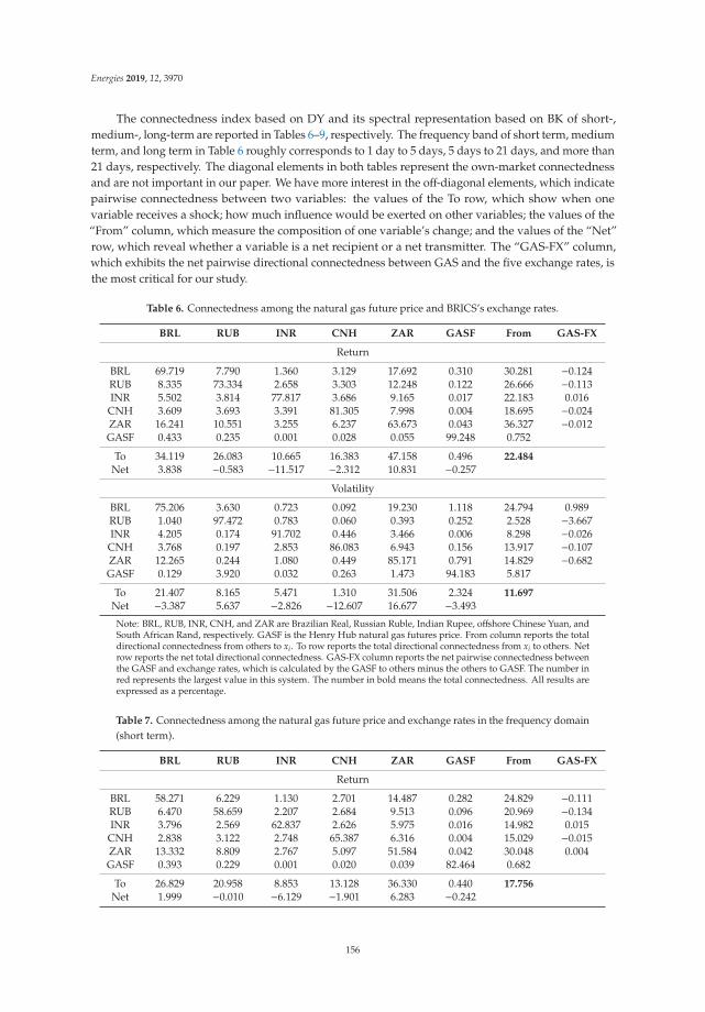
Energies 2019, 12, 3970

The connectedness index based on DY and its spectral representation based on BK of short-,medium-, long-term are reported in Tables 6–9, respectively. The frequency band of short term, mediumterm, and long term in Table 6 roughly corresponds to 1 day to 5 days, 5 days to 21 days, and more than21 days, respectively. The diagonal elements in both tables represent the own-market connectednessand are not important in our paper. We have more interest in the off-diagonal elements, which indicatepairwise connectedness between two variables: the values of the To row, which show when onevariable receives a shock; how much influence would be exerted on other variables; the values of the“From” column, which measure the composition of one variable’s change; and the values of the “Net”row, which reveal whether a variable is a net recipient or a net transmitter. The “GAS-FX” column,which exhibits the net pairwise directional connectedness between GAS and the five exchange rates, isthe most critical for our study.

Table 6. Connectedness among the natural gas future price and BRICS’s exchange rates.

BRL RUB INR CNH ZAR GASF From GAS-FX

Return

BRL 69.719 7.790 1.360 3.129 17.692 0.310 30.281 −0.124RUB 8.335 73.334 2.658 3.303 12.248 0.122 26.666 −0.113INR 5.502 3.814 77.817 3.686 9.165 0.017 22.183 0.016

CNH 3.609 3.693 3.391 81.305 7.998 0.004 18.695 −0.024ZAR 16.241 10.551 3.255 6.237 63.673 0.043 36.327 −0.012GASF 0.433 0.235 0.001 0.028 0.055 99.248 0.752

To 34.119 26.083 10.665 16.383 47.158 0.496 22.484

Net 3.838 −0.583 −11.517 −2.312 10.831 −0.257

Volatility

BRL 75.206 3.630 0.723 0.092 19.230 1.118 24.794 0.989RUB 1.040 97.472 0.783 0.060 0.393 0.252 2.528 −3.667INR 4.205 0.174 91.702 0.446 3.466 0.006 8.298 −0.026

CNH 3.768 0.197 2.853 86.083 6.943 0.156 13.917 −0.107ZAR 12.265 0.244 1.080 0.449 85.171 0.791 14.829 −0.682GASF 0.129 3.920 0.032 0.263 1.473 94.183 5.817

To 21.407 8.165 5.471 1.310 31.506 2.324 11.697

Net −3.387 5.637 −2.826 −12.607 16.677 −3.493

Note: BRL, RUB, INR, CNH, and ZAR are Brazilian Real, Russian Ruble, Indian Rupee, offshore Chinese Yuan, andSouth African Rand, respectively. GASF is the Henry Hub natural gas futures price. From column reports the totaldirectional connectedness from others to xi. To row reports the total directional connectedness from xi to others. Netrow reports the net total directional connectedness. GAS-FX column reports the net pairwise connectedness betweenthe GASF and exchange rates, which is calculated by the GASF to others minus the others to GASF. The number inred represents the largest value in this system. The number in bold means the total connectedness. All results areexpressed as a percentage.

Table 7. Connectedness among the natural gas future price and exchange rates in the frequency domain(short term).


Return

BRL 58.271 6.229 1.130 2.701 14.487 0.282 24.829 −0.111RUB 6.470 58.659 2.207 2.684 9.513 0.096 20.969 −0.134INR 3.796 2.569 62.837 2.626 5.975 0.016 14.982 0.015

CNH 2.838 3.122 2.748 65.387 6.316 0.004 15.029 −0.015ZAR 13.332 8.809 2.767 5.097 51.584 0.042 30.048 0.004GASF 0.393 0.229 0.001 0.020 0.039 82.464 0.682

To 26.829 20.958 8.853 13.128 36.330 0.440 17.756

Net 1.999 −0.010 −6.129 −1.901 6.283 −0.242

156

Energies 2019, 12, 3970

Table 7. Cont.


Volatility

BRL 2.783 0.001 0.027 0.000 0.193 0.001 0.222 −0.001RUB 0.002 1.226 0.011 0.000 0.022 0.000 0.036 −0.010INR 0.012 0.006 1.107 0.006 0.039 0.001 0.063 −0.002

CNH 0.012 0.000 0.029 5.085 0.057 0.005 0.103 0.003ZAR 0.085 0.012 0.019 0.004 1.181 0.000 0.120 −0.007GASF 0.001 0.010 0.004 0.002 0.008 3.005 0.025

To 0.112 0.030 0.090 0.012 0.319 0.008 0.095

Net −0.110 −0.006 0.026 −0.091 0.199 −0.017

Note: BRL, RUB, INR, CNH, and ZAR are Brazilian Real, Russian Ruble, Indian Rupee, offshore Chinese Yuan, andSouth African Rand, respectively. GASF is the Henry Hub natural gas futures price. From column reports the totaldirectional connectedness from others to xi. To row reports the total directional connectedness from xi to others.Net row reports the net total directional connectedness. GAS-FX column reports the net pairwise connectednessbetween the GASF and exchange rates, which is calculated by the GASF to others minus the others to GASF. Thenumber in red represents the largest value in this system. The number in bold means the total connectedness. Thefrequency band of short term roughly corresponds to 1 day to 5 days. All results are expressed as a percentage.

Table 8. Connectedness among the natural gas future price and exchange rates in the frequency domain(medium term).


Return

BRL 8.454 1.149 0.170 0.318 2.363 0.020 4.020 −0.009RUB 1.372 10.802 0.334 0.457 2.011 0.019 4.193 0.015INR 1.250 0.912 11.041 0.777 2.332 0.001 5.272 0.001

CNH 0.567 0.423 0.474 11.721 1.237 0.000 2.701 −0.006ZAR 2.148 1.289 0.361 0.840 8.913 0.001 4.639 −0.011GASF 0.030 0.005 0.000 0.006 0.012 12.391 0.053

To 5.367 3.777 1.339 2.398 7.956 0.042 3.480

Net 1.347 −0.416 −3.933 −0.303 3.316 −0.012

Volatility

BRL 8.452 0.018 0.091 0.002 0.712 0.006 0.829 −0.002RUB 0.012 4.530 0.035 0.000 0.082 0.002 0.130 −0.059INR 0.072 0.034 4.791 0.020 0.193 0.001 0.320 −0.003

CNH 0.075 0.001 0.093 15.124 0.275 0.009 0.452 0.004ZAR 0.273 0.036 0.062 0.004 3.877 0.001 0.375 −0.032GASF 0.008 0.061 0.005 0.005 0.033 9.896 0.111

To 0.440 0.150 0.285 0.029 1.296 0.019 0.370

Net −0.389 0.020 −0.035 −0.423 0.920 −0.092

Note: BRL, RUB, INR, CNH, and ZAR are Brazilian Real, Russian Ruble, Indian Rupee, offshore Chinese Yuan, andSouth African Rand, respectively. GASF is the Henry Hub natural gas future price. From column reports the totaldirectional connectedness from others to xi. To row reports the total directional connectedness from xi to others. Netrow reports the net total directional connectedness. GAS-FX column reports the net pairwise connectedness betweenthe GASF and exchange rates, which is calculated by the GASF to others minus the others to GASF. The number inred represents the largest value in this system. The number in bold means the total connectedness. The frequencyband of medium term roughly corresponds to 5 days to 21 days. All results are expressed as a percentage.

157

Energies 2019, 12, 3970

Table 9. Connectedness among the natural gas future price and exchange rates in the frequency domain(long term).


Return

BRL 2.994 0.412 0.060 0.111 0.842 0.007 1.432 −0.003RUB 0.493 3.873 0.118 0.162 0.724 0.007 1.504 0.006INR 0.456 0.333 3.940 0.282 0.857 0.000 1.929 0.000

CNH 0.204 0.148 0.169 4.198 0.444 0.000 0.965 −0.002ZAR 0.761 0.453 0.126 0.299 3.176 0.000 1.640 −0.004GASF 0.010 0.001 0.000 0.002 0.004 4.392 0.017

To 1.923 1.347 0.473 0.857 2.872 0.014 1.248

Net 0.491 −0.157 −1.455 −0.108 1.232 −0.003

Volatility

BRL 63.970 3.611 0.606 0.090 18.324 1.111 23.742 0.991RUB 1.026 91.716 0.737 0.059 0.289 0.250 2.361 −3.598INR 4.121 0.134 85.804 0.421 3.235 0.003 7.914 −0.020

CNH 3.681 0.196 2.731 65.874 6.611 0.142 13.361 −0.114ZAR 11.906 0.196 1.000 0.442 80.113 0.790 14.334 −0.642GASF 0.120 3.848 0.023 0.257 1.432 81.282 5.680

To 20.855 7.985 5.097 1.269 29.891 2.297 11.232

Net −2.888 5.624 −2.817 −12.093 15.558 −3.384

Note: BRL, RUB, INR, CNH, and ZAR are Brazilian Real, Russian Ruble, Indian Rupee, offshore Chinese Yuan, andSouth African Rand, respectively. GASF is the Henry Hub natural gas future price. From column reports the totaldirectional connectedness from others to xi. To row reports the total directional connectedness from xi to others. Netrow reports the net total directional connectedness. GAS-FX column reports the net pairwise connectedness betweenthe GASF and exchange rates, which is calculated by the GASF to others minus the others to GASF. The number inred represents the largest value in this system. The number in bold means the total connectedness. The frequencyband of long term roughly corresponds to more than 21 days. All results are expressed as percentages.

As shown in Table 6, the total connectedness of the return series is 22.484%, which is almosttwice as much as the connectedness between volatilities (11.697%), but both of them are modest.In this system, no matter what the connectedness from the return series or volatilities was, the shockstransmitted from ZAR to BRL contributed the largest value. The BRL was a net transmitter in returnconnectedness, but a net recipient in volatility connectedness. The RUB was opposite to BRL in that itwas a net recipient in the return case, but a net transmitter in the volatility case. Furthermore, INR,CNH, and GASF were net receivers in both cases, whereas ZAR was a net transmitter. By obtainingthe absolute value of the “Net” row, we found that INR had the strongest influence (11.517%) in allreturn series and ZAR was the most powerful variable (16.677%) in volatilities.

In Tables 7–9, we note that the sum of total connectedness in the short term, medium term, andlong term is equal to the total connectedness shown in Table 6, which is in agreement with the definitionof frequency decomposition for connectedness. It is interesting to find that the total connectednessfrom the return series is highest in the short term (17.756%), followed by the medium term (3.480%)and long term (1.248%). By contrast, from volatilities, the value is highest in the long term (11.232%),followed by the medium term (0.370%) and short term (0.095%), which means that the uncertaintytransmitted by the shock has a long-term impact on the market, rather than the shock itself.

From the values of the GAS-FX column, we found that the net pairwise connectedness betweenGAS and the exchange rate was higher in volatilities than return series, but both were very weak.All values were almost zero. The possible reason for this is that the GASF data we have chosen arefor Henry Hub natural gas, which could be seen as representative of the North American natural gasmarket. However, as the natural gas pipeline in North America can hardly reach any BRICS countries,and the distance between North America and BRICS countries makes the transportation cost of LNGexpensive, whether as an import or export, North American natural gas is not the primary selection for

158

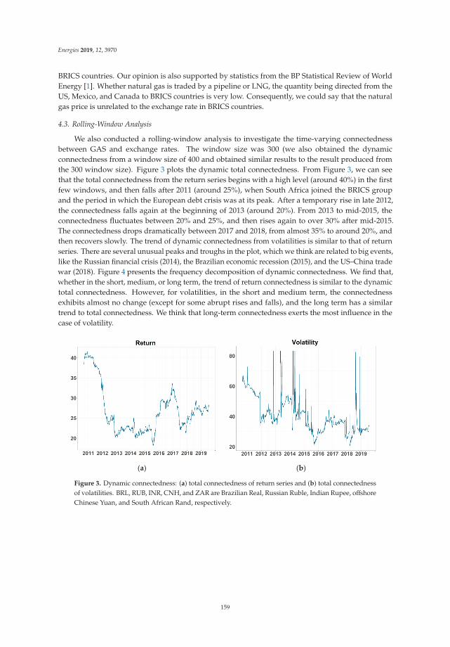
Energies 2019, 12, 3970

BRICS countries. Our opinion is also supported by statistics from the BP Statistical Review of WorldEnergy [1]. Whether natural gas is traded by a pipeline or LNG, the quantity being directed from theUS, Mexico, and Canada to BRICS countries is very low. Consequently, we could say that the naturalgas price is unrelated to the exchange rate in BRICS countries.

4.3. Rolling-Window Analysis

We also conducted a rolling-window analysis to investigate the time-varying connectednessbetween GAS and exchange rates. The window size was 300 (we also obtained the dynamicconnectedness from a window size of 400 and obtained similar results to the result produced fromthe 300 window size). Figure 3 plots the dynamic total connectedness. From Figure 3, we can seethat the total connectedness from the return series begins with a high level (around 40%) in the firstfew windows, and then falls after 2011 (around 25%), when South Africa joined the BRICS groupand the period in which the European debt crisis was at its peak. After a temporary rise in late 2012,the connectedness falls again at the beginning of 2013 (around 20%). From 2013 to mid-2015, theconnectedness fluctuates between 20% and 25%, and then rises again to over 30% after mid-2015.The connectedness drops dramatically between 2017 and 2018, from almost 35% to around 20%, andthen recovers slowly. The trend of dynamic connectedness from volatilities is similar to that of returnseries. There are several unusual peaks and troughs in the plot, which we think are related to big events,like the Russian financial crisis (2014), the Brazilian economic recession (2015), and the US–China tradewar (2018). Figure 4 presents the frequency decomposition of dynamic connectedness. We find that,whether in the short, medium, or long term, the trend of return connectedness is similar to the dynamictotal connectedness. However, for volatilities, in the short and medium term, the connectednessexhibits almost no change (except for some abrupt rises and falls), and the long term has a similartrend to total connectedness. We think that long-term connectedness exerts the most influence in thecase of volatility.

(a) (b)

Figure 3. Dynamic connectedness: (a) total connectedness of return series and (b) total connectednessof volatilities. BRL, RUB, INR, CNH, and ZAR are Brazilian Real, Russian Ruble, Indian Rupee, offshoreChinese Yuan, and South African Rand, respectively.

159

Energies 2019, 12, 3970

(a) (b)

Figure 4. Frequency decomposition of dynamic connectedness: (a) frequency decomposition of totalconnectedness for return series and (b) frequency decomposition of total connectedness for volatilities.Note: BRL, RUB, INR, CNH, and ZAR are Brazilian Real, Russian Ruble, Indian Rupee, offshoreChinese Yuan, and South African Rand, respectively. GASF is the Henry Hub natural gas futures price.

The time-varying net pairwise connectedness between GAS and exchange rates return seriesis plotted in Figure 5. Like the result in Section 4.2, all values were low and almost all of themwere below 2.5% in terms of the absolute value, so were negligible. The results from volatilities arepresented in Figure 6. There are also several sudden rises and falls, which is consistent with the plotof total connectedness. In the net pairwise connectedness of GAS-BRL, GAS-INR, and GAS-ZARpairs, except for the abnormal value at some points, the values were almost insignificant; thus, we canhardly say that the GAS has an influence on the exchange rate or vice versa. However, in GAS-RUBand GAS-CNH pairs, there are some significant positive or negative periods during our data span.Before 2014, GAS was a net transmitter to RUB, and then turned into a net recipient after 2014, whenRussia was undergoing an economic crisis caused by the oil price crash. After 2016, GAS was a nettransmitter to CNH, when Australia became the largest supplier of LNG to China instead of Qatar, andthe trade kept increasing after that.

160

Energies 2019, 12, 3970

(a) (b)

(c) (d)

(e)

Figure 5. Net pairwise connectedness of return series. (a–e) refer to the net pairwise connectednessbetween GASF and BRL, RUB, INR, CNH, and ZAR return series, respectively. Note: BRL, RUB, INR,CNH, and ZAR are Brazilian Real, Russian Ruble, Indian Rupee, offshore Chinese Yuan, and SouthAfrican Rand, respectively. GASF is the Henry Hub natural gas futures price.

161

Energies 2019, 12, 3970

(a) (b)

(c) (d)

(e)

Figure 6. Net pairwise connectedness of volatility. (a–e) refer to net pairwise connectedness betweenthe volatility of GASF and BRL, RUB, INR, CNH, and ZAR, respectively. Note: BRL, RUB, INR, CNH,and ZAR are Brazilian Real, Russian Ruble, Indian Rupee, offshore Chinese Yuan, and South AfricanRand, respectively. GASF is the Henry Hub natural gas futures price.

5. Conclusions

This paper examined the connectedness between the Henry Hub natural gas price and the BRICS’sexchange rates. To that end, the connectedness methodology from Diebold and Yilmaz (2009, 2012,2015) as well as frequency decomposition of connectedness proposed by Baruník and Krehlík (2018)were used. We collected data from 23 August 2010 to 20 June 2019 and tested both return series andvolatilities from GARCH models.

162

Energies 2019, 12, 3970

Our empirical results show that the total connectedness was 22.5% in the return series and 11.7%in volatilities. Compared to results from previous studies—such as Lundgren et al. [13] who found thatthe total volatility connectedness among renewable energy stock returns, investment assets, and severalsources of uncertainty is 67.4%—our results are modest, which means that most variation was due tothe variation in the variables themselves. By taking the frequency decomposition of connectedness,we found that, in the return series, the short term contributes to the total connectedness the most,whereas the long term contributes most in relation to volatility. From the results of net pairwiseconnectedness between the natural gas price and exchange rates, we obtained a value of almost zero ineach natural gas and exchange rate pair, which means that natural gas does not play an importantrole in explaining movements in the exchange rates. We also applied a rolling-window approach toconduct the time-varying analysis. In short, the results are similar to those of the constant analysis andwe cannot say for certain that the natural gas price had a great influence on exchange rate movement.Only in the plot of volatility connectedness were there several dramatic fluctuations, which we considerto be connected to some notable events, such as economic crises and trade frictions.

Our results are obviously different from the results of the studies on the relationship between theoil price and exchange rates, such as that conducted by Singh et al. (2018), who found that the totalvolatility connectedness between the oil price and nine exchange rates reached 72.96%. The shockstransmitted from crude oil to each exchange rate are also significant. We consider some possiblereasons for the difference. First, crude oil can be used more widely across different fields than naturalgas. For example, it can fuel our cars and make plastics, rubbers, and the like, which are uses thatcannot be replaced by natural gas. As indicated in the BP Statistical Review of World Energy [1], crudeoil has the highest share in global energy consumption, and its consumption is almost double that ofnatural gas. Second, the production of crude oil far exceeds that of natural gas. Therefore, whether forenergy import countries or energy export countries, crude oil is more easily traded. Third, comparedto developed countries, awareness of the environment in developing countries is at a lower level.As the BRICS are the focus of our study, although their consumption of natural gas has increased inrecent years, natural gas is still not the primary energy source for these countries (with the exception ofRussia). India, China, and South Africa consumed coal the most in 2019, while Brazil consumed oil themost [1].

Although crude oil plays an irreplaceable role in the energy market now, with increasingenvironmental awareness, we believe that natural gas will become more important and theconnectedness between the natural gas price and exchange rates will become stronger in the future.

The empirical evidence in this study may have important implications for policymakers, especiallythose in oil-dependent countries. As much of the literature shows that exchange rates are highlydependent on the oil price, turbulence in the crude oil market could have a great impact on the foreigncurrency market, thus causing exchange rate pressure and even economic instability. In order tosolve the foreign exchange fluctuation, monetary authorities need to accumulate or reduce foreignexchange reserves, which is not considered desirable in the real world. Changing the dependencestructure in relation to energy—from depending on energy that is closely connected with the currencymarket, such as crude oil, to depending on energy that is hardly connected to the currency market,such as natural gas—could provide an efficient way of maintaining economic stability and reducingexchange rate pressure. By contrast, because of the low connectedness between the natural gas priceand exchange rates, foreign exchange fluctuation may barely be affected by the natural gas price.Therefore, for investors, it is less risky to invest in gas-related financial products than oil-relatedfinancial products, which are highly connected with currency.

Although this paper conducted thorough research, there were several limitations in the empiricalwork. First, although we found that natural gas did not have a significant impact on the exchangerate, this result could be influenced by the data selection. We used Henry Hub as our natural gas pricedata, which represents the North American natural gas market. However, given the restriction ofpipelines and high transportation cost, North American countries that produce natural gas may not

163

Energies 2019, 12, 3970

be the primary selection for BRICS. Second, with technological improvements in exploiting naturalgas and the increasing number of gas liquefaction plants, we assumed that the LNG price wouldhave more influence on the exchange rate than the pipeline natural gas price did. However, owingto data limitations, we could only focus on the whole natural gas market, which may be the reasonwhy the connectedness between the natural gas price and exchange rates was modest. Therefore, forfurther extension of this research, first, we want to collect different natural gas price data, such as theNetherlands Title Transfer Facility (TTF) index and Japan Korea Marker, to exclude the impact of dataselection on the results. Second, we want to analyze the relationship between the crude oil price andexchange rates and the relationship between the crude oil price and natural gas price. This would allowus to compare the connectedness between the crude oil price and exchange rates with that between thenatural gas price and exchange rates more rationally. Finally, if the data permit, we want to use thedata on only LNG to find the connectedness between the natural gas price and foreign exchange ratesmore precisely.

Author Contributions: Conceptualization, S.H.; investigation, Y.H.; writing—original draft preparation, Y.H.;writing—review and editing, T.N.; project administration, S.H.; funding acquisition, S.H.



Conflicts of Interest: The authors declare no conflicts of interest.

Appendix A Robustness Analysis

We used the Henry Hub natural gas spot price (GASS) as the natural gas price data to examinethe robustness of our results. (The natural gas futures index in the United Kingdom, which is knownas the UK National Balancing Point (NBP), was also used to conduct the robustness check, but theresults were quite similar to those from GASS, so we only present the connectedness table of NBP andexchange rates (Table A2) in Appendix A).

The plot of GASS’s return and volatility series are reported in Figure A1. We found that somevalues of volatility were extremely large (the maximum is over 800). We think that the reason for this isthat the natural gas spot price was more easily affected by the change of demand and supply than thefuture price, even though the change was small.

We summarize the results of connectedness and the frequency decomposition of short, medium,and long term in Table A1, Table A3, Table A4, Table A5, respectively. The result is quite similar tothat of GASF and exchange rates. We also used a 300 rolling-window to conduct the time-varyinganalysis. The dynamic connectedness and its spectral representation are plotted in Figures A2 and A3,respectively. The net pairwise connectedness of return series and volatilities are illustrated in Figures A4and A5, respectively. All results are consistent with those from the analysis using the natural gasfuture price, except for the net pairwise connectedness of return series (Figure A4). Some values areopposite to the result above, but all of them are low, even the maximum value, which is less than 5%and negligible.

The results of robustness confirm the suitability of our proposed approach, which aimed to capturethe relationship between the natural gas price and exchange rates.

164

Energies 2019, 12, 3970

Table A1. Connectedness between the natural gas spot price and BRICS’s exchange rates.

BRL RUB INR CNH ZAR GASS From GAS-FX

Return

BRL 69.839 7.714 1.456 3.124 17.688 0.179 30.161 −0.249RUB 8.323 73.405 2.681 3.276 12.230 0.085 26.595 −0.058INR 5.571 3.833 77.727 3.652 9.066 0.152 22.273 0.040

CNH 3.588 3.648 3.378 81.296 7.953 0.137 18.704 0.136ZAR 16.233 10.559 3.252 6.206 63.643 0.108 36.357 0.094GASS 0.429 0.143 0.113 0.001 0.014 99.301 0.699

To 34.143 25.896 10.879 16.259 46.951 0.660 22.465

Net 3.983 −0.699 −11.394 −2.444 10.593 −0.039

Volatility

BRL 75.533 3.660 0.288 0.354 20.138 0.025 24.467 −0.377RUB 0.890 97.569 0.750 0.298 0.479 0.014 2.431 −0.006INR 3.133 0.494 92.791 0.277 3.235 0.070 7.209 −0.234

CNH 3.679 0.213 2.713 85.576 7.123 0.696 14.424 0.678ZAR 11.251 0.282 0.801 1.067 86.363 0.236 13.637 0.208GASS 0.402 0.020 0.304 0.018 0.028 99.229 0.771

To 19.356 4.669 4.856 2.015 31.003 1.041 10.490

Net −5.111 2.238 −2.354 −12.410 17.367 0.270

Note: BRL, RUB, INR, CNH, and ZAR are Brazilian Real, Russian Ruble, Indian Rupee, offshore Chinese Yuan, andSouth African Rand, respectively. GASF is the Henry Hub natural gas futures price. From column reports the totaldirectional connectedness from others to xi. To row reports the total directional connectedness from xi to others.Net row reports the net total directional connectedness. GAS-FX column reports the net pairwise connectednessbetween the GASS and exchange rates, which is calculated by the GASS to others minus the others to GASS. Thenumber in red represents the largest value in this system. The number in bold means the total connectedness. Allresults are expressed as a percentage.

Table A2. Connectedness between the UK NBP and BRICS’s exchange rates.


Return

BRL 69.761 7.791 1.352 3.139 17.707 0.249 30.239 −0.099RUB 8.337 73.395 2.660 3.307 12.251 0.049 26.605 −0.014INR 5.472 3.796 77.446 3.686 9.115 0.485 22.554 0.134

CNH 3.600 3.676 3.391 80.904 7.971 0.458 19.096 −0.088ZAR 16.162 10.491 3.227 6.215 63.346 0.559 36.654 −0.286GASS 0.348 0.062 0.352 0.546 0.845 97.847 2.153

To 33.919 25.816 10.983 16.893 47.889 1.800 22.883

Net 3.680 −0.788 −11.571 −2.204 11.236 −0.353

Volatility

BRL 75.164 3.509 0.542 0.277 20.254 0.254 24.836 −0.041RUB 0.947 96.034 0.952 0.188 0.549 1.329 3.966 1.213INR 3.494 0.244 90.752 0.328 3.404 1.778 9.248 −1.243

CNH 3.879 0.269 2.684 85.577 6.804 0.788 14.423 0.611ZAR 11.028 0.318 0.775 0.822 86.380 0.677 13.620 −0.742GASS 0.295 0.116 3.021 0.177 1.419 94.971 5.029

To 19.643 4.456 7.974 1.792 32.430 4.827 11.854

Net −5.193 0.491 −1.274 −12.631 18.810 −0.202

Note: BRL, RUB, INR, CNH, and ZAR are Brazilian Real, Russian Ruble, Indian Rupee, offshore Chinese Yuan,and South African Rand, respectively. NBP is the UK National Balancing Point. From column reports the totaldirectional connectedness from others to xi. To row reports the total directional connectedness from xi to others.Net row reports the net total directional connectedness. GAS-FX column reports the net pairwise connectednessbetween the NBP and exchange rates, which is calculated by the NBP to others minus the others to NBP. The numberin red represents the largest value in this system. The number in bold means the total connectedness. All results areexpressed as a percentage.

165

Energies 2019, 12, 3970

Table A3. Connectedness between the natural gas spot price and exchange rates in the frequencydomain (short term).


Return

BRL 58.953 6.079 1.107 2.772 14.530 0.118 24.606 −0.295RUB 6.713 58.808 2.160 2.705 9.511 0.057 21.146 −0.060INR 4.027 2.716 64.161 2.696 6.053 0.150 15.641 0.075

CNH 2.969 3.124 2.809 66.238 6.361 0.096 15.357 0.095ZAR 13.475 8.616 2.769 5.042 51.620 0.089 29.991 0.081GASS 0.414 0.118 0.075 0.001 0.008 81.932 0.615

To 27.597 20.653 8.919 13.216 36.463 0.510 17.893Net 2.991 −0.494 −6.722 −2.141 6.472 −0.106

Volatility

BRL 2.698 0.002 0.028 0.002 0.205 0.002 0.238 −0.003RUB 0.001 1.256 0.011 0.002 0.026 0.001 0.041 −0.003INR 0.016 0.009 1.099 0.006 0.030 0.000 0.061 −0.001

CNH 0.010 0.002 0.022 5.130 0.056 0.004 0.093 0.001ZAR 0.090 0.011 0.014 0.006 1.193 0.000 0.121 −0.001GASS 0.005 0.004 0.001 0.004 0.001 8.637 0.015

To 0.123 0.028 0.076 0.019 0.318 0.007 0.095

Net −0.116 −0.014 0.015 −0.075 0.197 −0.008

Note: The frequency band of short term roughly corresponds to 1 day to 5 days. All results are expressed as apercentage. Note: BRL, RUB, INR, CNH, and ZAR are Brazilian Real, Russian Ruble, Indian Rupee, offshore ChineseYuan, and South African Rand, respectively. GASF is the Henry Hub natural gas futures price.

Table A4. Connectedness between the natural gas spot price and exchange rates in the frequencydomain (medium term).


Return

BRL 8.061 1.197 0.254 0.265 2.325 0.045 4.086 0.032RUB 1.195 10.750 0.382 0.423 1.997 0.020 4.018 0.001INR 1.143 0.821 10.068 0.705 2.216 0.003 4.888 −0.025

CNH 0.465 0.392 0.426 11.137 1.177 0.030 2.489 0.030ZAR 2.045 1.423 0.359 0.856 8.868 0.014 4.697 0.010GASS 0.013 0.019 0.028 0.000 0.004 13.017 0.065

To 4.861 3.852 1.448 2.250 7.720 0.113 3.374

Net 0.775 −0.166 −3.440 −0.240 3.023 0.048

Volatility

BRL 9.181 0.005 0.052 0.020 1.331 0.005 1.413 −0.030RUB 0.007 3.981 0.043 0.013 0.090 0.002 0.155 −0.003INR 0.253 0.076 5.828 0.015 0.084 0.002 0.430 −0.012

CNH 0.090 0.003 0.086 14.160 0.385 0.093 0.657 0.087ZAR 0.486 0.050 0.049 0.005 4.430 0.006 0.596 0.002GASS 0.036 0.005 0.014 0.007 0.004 35.740 0.065

To 0.872 0.139 0.244 0.059 1.894 0.108 0.553

Net −0.541 −0.016 −0.186 −0.598 1.298 0.044

Note: The frequency band of medium term roughly corresponds to 5 days to 21 days. All results are expressedas a percentage. Note: BRL, RUB, INR, CNH, and ZAR are Brazilian Real, Russian Ruble, Indian Rupee, offshoreChinese Yuan, and South African Rand, respectively. GASF is the Henry Hub natural gas futures price.

166

Energies 2019, 12, 3970

Table A5. Connectedness between the natural gas spot price and exchange rates in the frequencydomain (long term).


Return

BRL 2.825 0.437 0.095 0.087 0.833 0.016 1.468 0.014RUB 0.415 3.847 0.138 0.149 0.722 0.007 1.431 0.001INR 0.401 0.296 3.498 0.250 0.797 0.000 1.744 −0.010

CNH 0.155 0.132 0.144 3.921 0.415 0.010 0.857 0.010ZAR 0.713 0.520 0.124 0.308 3.155 0.005 1.669 0.003GASS 0.001 0.006 0.010 0.000 0.002 4.352 0.019

To 1.685 1.391 0.512 0.793 2.769 0.038 1.198

Net 0.217 −0.040 −1.232 −0.063 1.099 0.019

Volatility

BRL 63.654 3.654 0.208 0.333 18.603 0.018 22.815 −0.343RUB 0.882 92.332 0.696 0.283 0.362 0.011 2.234 0.001INR 2.864 0.409 85.864 0.257 3.121 0.068 6.719 −0.221

CNH 3.580 0.209 2.605 66.285 6.682 0.598 13.674 0.591ZAR 10.675 0.220 0.738 1.056 80.740 0.230 12.919 0.207GASS 0.361 0.011 0.289 0.008 0.023 54.851 0.691

To 18.362 4.502 4.535 1.937 28.790 0.926 9.842

Net −4.454 2.268 −2.183 −11.737 15.872 0.235

Note: The frequency band of long term roughly corresponds to more than 21 days. All results are expressed asa percentage. Note: BRL, RUB, INR, CNH, and ZAR are Brazilian Real, Russian Ruble, Indian Rupee, offshoreChinese Yuan, and South African Rand, respectively. GASF is the Henry Hub natural gas futures price.

(a) (b)

Figure A1. Daily return and volatility: (a) return series and (b) volatility.

167

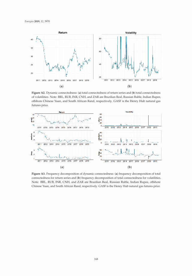
Energies 2019, 12, 3970

(a) (b)

Figure A2. Dynamic connectedness: (a) total connectedness of return series and (b) total connectednessof volatilities. Note: BRL, RUB, INR, CNH, and ZAR are Brazilian Real, Russian Ruble, Indian Rupee,offshore Chinese Yuan, and South African Rand, respectively. GASF is the Henry Hub natural gasfutures price.

(a) (b)

Figure A3. Frequency decomposition of dynamic connectedness: (a) frequency decomposition of totalconnectedness for return series and (b) frequency decomposition of total connectedness for volatilities.Note: BRL, RUB, INR, CNH, and ZAR are Brazilian Real, Russian Ruble, Indian Rupee, offshoreChinese Yuan, and South African Rand, respectively. GASF is the Henry Hub natural gas futures price.

168

Energies 2019, 12, 3970

(a) (b)

(c) (d)

(e)

Figure A4. Net pairwise connectedness of return series: (a–e) refer to the net pairwise connectednessbetween GASS and BRL, RUB, INR, CNH, and ZAR return series, respectively. Note: BRL, RUB, INR,CNH, and ZAR are Brazilian Real, Russian Ruble, Indian Rupee, offshore Chinese Yuan, and SouthAfrican Rand, respectively. GASF is the Henry Hub natural gas futures price.

169

Energies 2019, 12, 3970

(a) (b)

(c) (d)

(e)

Figure A5. Net pairwise connectedness of volatility. (a–e) refer to the net pairwise connectednessbetween the volatility of GASS and BRL, RUB, INR, CNH, and ZAR, respectively. Note: BRL, RUB,INR, CNH, and ZAR are Brazilian Real, Russian Ruble, Indian Rupee, offshore Chinese Yuan, andSouth African Rand, respectively. GASF is the Henry Hub natural gas futures price.

References

1. BP p.l.c. BP Statistical Review of World Energy 2019. Available online: https://www.bp.com/content/dam/bp/business-sites/en/global/corporate/pdfs/energy-economics/statistical-review/bp-stats-review-2019-full-report.pdf (accessed on 1 July 2019).

2. Mckinsey & Company. Global Energy Perspective 2019: Reference Case. Available online:https://www.mckinsey.com/~{}/media/McKinsey/Industries/Oil%20and%20Gas/Our%20Insights/

170

Energies 2019, 12, 3970

Global%20Energy%20Perspective%202019/McKinsey-Energy-Insights-Global-Energy-Perspective-2019_Reference-Case-Summary.ashx (accessed on 22 September 2019).

3. International Energy Agency. World Energy Outlook 2018. 2018. Available online: https://www.iea.org/weo/(accessed on 22 September 2019).

4. Diebold, F.X.; Yilmaz, K. Measuring Financial Asset Return and Volatility Spillovers, with Application toGlobal Equity Market. Econ. J. 2009, 119, 158–171. [CrossRef]

5. Diebold, F.X.; Yilmaz, K. Better to give than to receive: Predictive directional measurement of volatilityspillovers. Int. J Forecast. 2012, 28, 57–66. [CrossRef]

6. Diebold, F.X.; Yilmaz, K. Financial and Macroeconomic Connectedness: A Network Approach to Measurement andMonitoring; Oxford University Press: Oxford, UK, 2015.

7. Baruník, J.; Krehlík, T. Measuring the Frequency Dynamics of Financial Connectedness and Systemic Risk.J. Financ. Econ. 2018, 16, 271–296. [CrossRef]

8. Chen, S.-S.; Chen, H.-C. Oil prices and real exchange rates. Energy Econ. 2007, 29, 390–404. [CrossRef]9. Andries, , A.M.; Ihnatov, I.; Tiwari, A.K. Analyzing time–frequency relationship between interest rate, stock

price and exchange rate through continuous wavelet. Econ. Model. 2014, 41, 227–238. [CrossRef]10. Brahm, T.; Huang, J.-C.; Sissoko, Y. Crude oil prices and exchange rates: Causality, variance decomposition

and impulse response. Energy Econ. 2014, 44, 407–412.11. Jain, A.; Pratap, B. Dynamic linkages among oil price, gold price, exchange rate, and stock market in India.

Resour. Policy 2016, 49, 179–185. [CrossRef]12. Maghyereh, A.I.; Awartani, B.; Bouri, E. The directional volatility connectedness between crude oil and

equity markets: New evidence from implied volatility indexes. Energy Econ. 2016, 57, 78–93. [CrossRef]13. Lundgren, A.I.; Milicevic, A.; Uddin, G.S.; Kang, S.H. Connectedness network and dependence structure

mechanism in green investments. Energy Econ. 2018, 72, 145–153. [CrossRef]14. Singh, V.K.; Nishant, S.; Kumar, P. Dynamic and directional network connectedness of crude oil and

currencies: Evidence from implied volatility. Energy Econ. 2018, 76, 48–63. [CrossRef]15. Ji, Q.; Geng, J.B.; Tiwari, A.K. Information spillovers and connectedness networks in the oil and gas markets.

Energy Econ. 2018, 75, 71–84. [CrossRef]16. Lovch, Y.; Perez-Laborda, A. Dynamic frequency connectedness between oil and natural gas volatilities.

Econ. Model. 2019. [CrossRef]17. Sims, C.A. Macroeconomics and Reality. Econometrica 1980, 48, 1–48. [CrossRef]18. Koop, G.; Pesaran, M.H.; Potter, S.M. Impulse response analysis in nonlinear multivariate models. J. Econ.

1996, 74, 119–147. [CrossRef]19. Pesaran, H.H.; Shin, Y. Generalized impulse response analysis in linear multivariate models. Econ. Lett. 1998,

58, 17–29. [CrossRef]20. Lütkepohl, H. New Introduction to Multiple Time Series Analysis; Springer: Berlin/Heidelberg, Germany, 2005.21. Geweke, J. Measurement of Linear Dependence and Feedback between Multiple Time Series. J. Am.

Stat. Assoc. 1982, 77, 304–313. [CrossRef]22. Geweke, J. Measures of Conditional Linear Dependence and Feedback between Time Series. J. Am. Stat. Assoc.

1984, 79, 907–915. [CrossRef]23. Geweke, J. The Superneutrality of Money in the United States: An Interpretation of the Evidence. Econometrica

1986, 54, 1–21. [CrossRef]24. Stiassny, A. A spectral decomposition for structural VAR models. Empir. Econ. 1996, 21, 535–555. [CrossRef]25. Diebold, F.X.; Yilmaz, K. On the network topology of variance decompositions: Measuring the connectedness

of financial firms. J. Econ. 2011, 182, 119–134. [CrossRef]26. Perron, P. The great crash, the oil price shock, and the unit root hypothesis. Econometrica 1989, 57, 1361–1401.

[CrossRef]

171

Energies 2019, 12, 3970

27. Papell, D.H.; Lumsdaine, R.L. Multiple trend breaks and the unit-root hypothesis. Rev. Econ. Stat. 1997, 79,212–218.

28. Andrews, D.W.K.; Zivot, E. Further evidence on the great crash, the oil-price shock, and the unit-roothypothesis. J. Bus. Econ. Stat. 2002, 20, 25–44.


172

energies

Article

Measurement of Connectedness and FrequencyDynamics in Global Natural Gas Markets

Tadahiro Nakajima 1,2,* and Yuki Toyoshima 3

1 The Kansai Electric Power Company, Incorporated, Osaka 530-8270, Japan2 Graduate School of Economics, Kobe University, Kobe 657-8501, Japan3 Shinsei Bank, Limited, Tokyo 103-8303, Japan; [email protected]* Correspondence: [email protected]

Received: 11 September 2019; Accepted: 12 October 2019; Published: 16 October 2019

Abstract: We examine spillovers among the North American, European, and Asia–Pacific naturalgas markets based on daily data. We use daily natural gas price indexes from 2 February 2009 to28 February 2019 for the Henry Hub, National Balancing Point, Title Transfer Facility, and Japan KoreaMarker. The results of spillover analyses indicate the total connectedness of the return and volatilityseries to be 22.9% and 32.8%, respectively. In other words, volatility is more highly integrated thanreturns. The results of the spectral analyses indicate the spillover effect of the return series can largelybe explained by short-term factors, while that of the volatility series can be largely explained bylong-term factors. The results of the dynamic analyses with moving window samples do not indicatethat global gas market liquidity increases with the increasing spillover index. However, the resultsidentify the spillover effect fluctuation caused by demand and supply.

Keywords: spillover effect; market integration; natural gas market; time frequency dynamics

1. Introduction

The natural gas market has registered an expanding trend, because the fuel transition from coal tonatural gas is accelerating in both the industrial and power sectors to reduce greenhouse gas emissionsand prevent air pollution, as well as stagnant nuclear power generation. According to BP StatisticalReview of World Energy June 2019 [1], the total primary energy consumption in the world grewfrom 12.4 billion tonnes of oil equivalent (btoe) in 2011 to 13.9 btoe in 2018. Coal consumption wasalmost constant at 3.6 btoe, while natural gas consumption increased from 2.8 btoe to 3.3 btoe. As aresult, the composition ratio of natural gas increased from 22.4% to 23.9%, though the compositionratio of coal decreased from 30.5% to 27.2%. Besides the traditional gas-producing countries in theMiddle East and Southeast Asia, others have been increasing their presence as exporting countries,such as Australia (which has been developing large-scale gas wells, including unconventional gasfields) and the United States of America (USA) (which began to export liquefied natural gas (LNG)derived from shale gas). Furthermore, the development of gas fields has been promoted even inAfrica recently. Natural gas production skyrocketed from 28 million tonnes of oil equivalent (mtoe),457 mtoe, and 120 mtoe in 2011 to 112 mtoe, 715 mtoe, and 203 mtoe in 2018, in Australia, the USA,and all of Africa, respectively. On the other hand, consumption is skyrocketing in China and theMiddle East, in addition to steady consumption for the members of the Organisation for EconomicCo-operation and Development (OECD). Natural gas consumption increased from 24 mtoe, 168 mtoe,and 1142 mtoe in 2011 to 243 mtoe, 476 mtoe, and 1505 mtoe in 2018 in China, all of the Middle East,and the OECD countries.

In the European market, progress in the deregulation of gas business and the decreasing trend ofthe proportion of long-term contracts linked to crude oil prices has been activating an inter-marketarbitrage based on gas pipelines. Moreover, in the global market, the increase in the ratio of LNG to


Energies 2019, 12, 3927

total natural gas trading volumes, the accelerated removal of the destination restriction clause fromLNG sales contracts, and the decreasing trend for the percentage of long-term contracts linked to crudeoil prices are activating an intercontinental arbitrage based on LNG. As the proportion of spot tradingincreases, the liquidity of the natural gas market also increases significantly.

According to the Japan Fair Trade Commission of the Government of Japan [2], the natural gasmarket has not been flexible in terms of region, volume, and price, with the supply chain beingconsidered a special energy market. However, as the trading volume increases with the increase in thenumber of producing and/or consuming countries, gas market liquidity has also become higher. As aresult, the market is changing to a general commodity market.

Natural gas portfolio holders require both security and flexibility in terms of demand and supplybecause they have to invest heavily and trade globally. Therefore, they need to monitor the relationshipbetween international natural gas markets in terms of revenue and risk management. As such, we adoptthe spillover index developed by Diebold and Yilmaz [3] to measure return and volatility spilloversbetween natural gas price indexes in Europe, North America, and Asia Pacific.

Our expectations for measuring spillover effects between markets are twofold. First, we can easilygrasp the potential of a portfolio with a single index obtained by analyzing the relationship of returnand volatility between securities that make up that portfolio. We can also overview the potentialdownside risk of the portfolio without strictly measuring the value at risk and the expected shortfall bya Monte Carlo simulation. Second, we can respond to risks early by using the index as a predictive riskindicator. If we monitor the market that is the source of the spillover, investors can smoothly rebalancetheir portfolios.

We must test the stationarity of variables because Diebold and Yilmaz [3] develop the spilloverindex based on the vector moving average (VMA) representation of the vector autoregression (VAR)model. However, the approach proposed by Diebold and Yilmaz [3] is not the Granger–causality test,but just the quantification of the spillover effect. In other words, this technique does not assess whethersignificant information to predict returns and/or volatility exists, but only estimates how the variablesare mutually influential.

However, notwithstanding these limitations of the method, we can obtain not only academicfindings concerning the most remarkable transformation market, that is, the natural gas and LNGmarkets, but also useful information for practitioners, such as regulatory authorities, exchanges,consumers, and suppliers. Further, this index is extremely informative for long-term investment,daily trading, production, and risk management in operating companies that hold such a naturalgas portfolio.

In recent years, there have been increased studies on the natural gas market in the context ofde-CO2, the shale gas revolution, and increased liquidity. Kum et al. [4], Das et al. [5], and Bildirici andBakirtas [6] examine the relationship between natural gas consumption volume and macroeconomicindicators in major developed countries, emerging national economies, and a developing country.Acaravci et al. [7] investigates the relationship between natural gas prices and stock prices in Europeancountries. Nakajima and Hamori [8], Atil et al. [9], Perifanis et al. [10], Tiwari et al. [11], andXia et al. [12] analyze the relationship between natural gas prices and the other energy prices in theUSA. Batten et al. [13] study the relationship between Russian natural gas prices and other energy prices.These previous studies were conducted in the context of causality, spillover, and market integrationbetween natural gas and other economic variables. Moreover, Nakajima [14] argues whether profitscan be earned by statistical arbitrage between wholesale electricity futures and natural gas futures.

However, few studies have examined natural gas market integration. Olsen et al. [15], Scarcioffoloand Etienne [16], and Ren et al. [17] discuss the market integration in North America. Nick [18],Osicka et al. [19], and Bastianin et al. [20] examine the European natural gas market integration.Shi et al. [21] reveals the interrelationship of LNG prices in Asia. Furthermore, there are few studiesthat have investigated the natural gas market integration across several regions. Neumann [22] studiesthe relationship between European and North American markets. Chai et al. [23] study the relationship

174

Energies 2019, 12, 3927

between the Chinese and the global market. No research has examined the global natural gas marketintegration, with the exception of that by Silverstovs et al. [24], analyzing the cointegrated relationshipbetween North America, Europe, and Japan based on monthly data from before the shale gas revolution.No studies analyze the spillover effects between North American, European, and Asia-Pacific naturalgas markets based on daily data.

We adopt Diebold and Yilmaz’s [3] approach to examine spillovers between global natural gasprice indexes based on daily data. The correlation coefficient captures only phenomena that do notinclude the meaning of the relationship. Although the cointegration analysis and the Granger causalitytest lead to long-term equilibrium and forecast performance, it is difficult to grasp the whole picture ata glance in the case of many variables to be analyzed. Diebold and Yilmaz’s [3] approach capturesnot only pairwise connectedness but also total connectedness. Although Diebold and Yilmaz’s [3]approach is not suitable for dynamic descriptions such as multivariate generalized autoregressiveconditional heteroscedasticity (GARCH), it is possible to capture dynamic trends with moving windowsamples. Moreover, we spectrally decompose the Diebold and Yilmaz [3] index by Fourier transform.Baruník and Krehlík [25] utilized the same technique for the first time and later papers applied thisapproach to the energy market. For instance, Toyoshima and Hamori [26] measure the spillover indexfor global crude oil markets and decompose it into long-, medium-, and short-term factors. Ji et al. [27]examine the spillover effects between crude oil, heating oil, gasoline, and natural gas in North Americaand the United Kingdom.

Our contribution to the literature is threefold. The contributions of this paper relate to clarifyingthe relationships by measuring the connectedness and its frequency dynamics in the global gas market.First, we indicate no progressing integration of the global natural gas market, although we indicate thestrong spillover effect between European markets. Moreover, we indicate that the volatility is higherintegrated than returns. The Diebold and Yilmaz’s [3] approach indicates that the total connectednessof return and volatility is 22.9% and 32.8%, respectively, while each total connectedness is mostlydependent on the pairwise connectedness between European natural gas price indexes. Second, ourspectral analyses indicate that long-term factors contribute to volatility spillovers, while short-termfactors contribute to return spillovers. We argue that arbitrage might cause short-term return spilloversand long-term memory of volatility might cause long-term volatility spillovers. Finally, our rollinganalyses indicate that the above two characteristics continue. Moreover, we argue that regional climate,demand and supply, and incidents might make spillover effects larger or smaller.

The remainder of this paper is organized as follows. Section 2 describes the analyzed data, summarystatistics, and preliminary basic analyses. Section 3 explains the adopted methodology. Section 4presents the empirical results. Section 5 provides a summary of the findings and states conclusions.

2. Data and Preliminary Analyses

2.1. Data

We select natural gas price indicators for the North American, European, and Asia–Pacific markets.We use Henry Hub (HH) futures as the North American index. HH is the name of a distribution hub inLouisiana for the natural gas pipeline system in North America, referring to natural gas delivered atthat hub. HH futures are listed on the New York Mercantile Exchange. We adopt National BalancingPoint (NBP) and Title Transfer Facility (TTF) futures as the European index. NBP futures are futures ofnatural gas at a virtual trading location in the United Kingdom, being listed on the IntercontinentalExchange (ICE). This market is related to production in the North Sea gas field, which is trading withthe European continent by pipelines, and consumption within the United Kingdom. TTF futuresare the futures of natural gas at a virtual trading point in the Netherlands, being listed on the ICE.This market reflects the continental European market, which consists of trading by long-haul pipelinesand LNG. We utilize the Japan/Korea Marker (JKM) as the Asia-Pacific index, which is associatedwith the short-term trading market for LNG in the Asia–Pacific region. It is provided by Platts, which

175

Energies 2019, 12, 3927

assesses benchmark prices in physical energy markets. We obtain the daily data from February 2, 2009to February 28, 2019 from Bloomberg.

Figure 1 shows the time series for these indexes. First, HH fluctuates independently from the othervariables. Second, the two European indexes move together. Finally, JKM is linked to the Europeanmarket over a specific period. As a result of the Great East Japan Earthquake on 11 March 2011,the amount of power generated by nuclear power plants has decreased significantly in Japan. Thus, wecan assume that the Asia-Pacific LNG market was tight, and therefore the JKM was soaring. Moreover,these European indexes might have increased as a result of arbitrage trading with the Asia-PacificLNG market. HH’s downtrend around 2012 might be caused by the expectations of increased shalegas production, while the price spike in 2014 was caused by the North American cold wave.

Figure 1. Time series plots of natural gas price. (HH =Henry Hub, NBP =National Balancing Point,TTF = Title Transfer Facility, JKM = Japan/Korea Marker).

Table 1 presents the summary statistics of the return and volatility series of each index. There are2436 observations in each case. The JKM return series has a distribution biased to the right and theother series have distributions biased to the left, as skewness is negative only for the JKM return series.The kurtosis of all series are extremely large. In other words, all series have fat tail distributions. Wecan reject the hypothesis that each series is normally distributed by the Jarque-Bera statistics calculatedfrom the skewness and kurtosis of each series.

Table 1. Summary statistics.

StatisticReturn Volatility *

HenryHub(HH)

NationalBalancing

Point (NBP)

Title TransferFacility (TTF)

Japan/KoreaMarker (JKM)

HH NBP TTF JKM

Observations 2436 2436 2436 2436 2436 2436 2436 2436Mean 0.0% 0.0% 0.0% 0.0% 2.9% 2.3% 2.0% 1.3%

Median −0.1% −0.1% −0.1% −0.0% 2.7% 2.1% 1.8% 1.0%Maximum value 30.7% 42.9% 29.6% 15.4% 8.7% 11.2% 7.9% 10.4%Minimum value −16.5% −12.3% −12.0% −22.6% 1.3% 0.7% 0.7% 0.3%

Standard deviation 3.2% 2.7% 2.3% 1.7% 1.1% 1.0% 0.9% 0.8%Skewness 0.92 2.3 1.5 –0.9 1.5 1.6 1.3 3.0Kurtosis 10.0 35.0 21.0 31.3 6.5 9.0 5.6 21.2

Jarque–Bera 5358 106,011 33,912 81,799 2182 4654 1353 37,478(p-value) (0) (0) (0) (0) (0) (0) (0) (0)

*: calculated by the stochastic volatility (SV) model.

As described in Toyoshima and Hamori [26], let xt be a return with mean zero and varianceexp(ht). The SV model can be expressed as follows:

176

Energies 2019, 12, 3927

xt|ht ∼ N(0, exp(ht))

ht∣∣∣ht−1, μ, ϕ, στ ∼ N

(μ+ ϕ(ht−1 − μ), σ2

τ

)h0

∣∣∣μ, ϕ, στ ∼ N(μ, σ2

τ/(1−ϕ2

))where μ, ϕ, and στ are the level of log variance, the persistence of log variance, and the volatility of logvariance, respectively.

2.2. Preliminary Analyses

The condition for the VMA representation of the VAR model is that all variables are stationary.Accordingly, we test for the stationarity status of all series by the augmented Dickey–Fuller (ADF) test.Table 2 presents the results. The ADF test rejects the null hypothesis that all variables have a unit root.Therefore, we can utilize the VMA representation.

We estimate the coefficient of the diagonal Baba, Engle, Kraft, and Kroner (BEKK) GARCH modelto calculate the dynamic correlation coefficients. The BEKK model is one of several variations ofmultivariate GARCH models depending on the formulation of the time-varying variance–covariancematrix. The BEKK model was developed by Engle and Kroner [28], and it guarantees a positiveestimated variance. Moreover, the BEKK model can dynamically calculate the correlation coefficient.When there are k variables, the variance-covariance matrix Ht of the BEKK model is as follows:

Ht = L′L + M′εt−1ε′t−1M + N′Ht−1N (1)

where M and N are a k× k matrix, and L is a k× k symmetric matrix.

Table 2. Unit root tests.

Series Variables Exogenous ADF–t Value (p-Value)

Return

Henry Hub (HH) Constant −54.12 (0.000)Constant, Trend −54.11 (0.000)

National Balancing Point (NBP) Constant −48.85 (0.000)Constant, Trend −48.84 (0.000)

Title Transfer Facility (TTF) Constant −47.65 (0.000)Constant, Trend −47.64 (0.000)

Japan/Korea marker (JKM) Constant −19.70 (0.000)Constant, Trend −19.73 (0.000)

Volatility

HHConstant −5.13 (0.000)

Constant, Trend −5.31 (0.000)

NBPConstant −7.18 (0.000)


TTFConstant −6.29 (0.000)


JKM Constant −16.60 (0.000)Constant, Trend −16.85 (0.000)

We calculate the correlation coefficients over the entire period, namely from 2 February 2009 to28 February 2019, to understand the simultaneous relationship between variables as a phenomenon.Tables 3 and 4 present the correlation coefficients for the return and volatility series, respectively.The correlation coefficient between the NBP and TTF is the largest for both the return and volatilityseries. Furthermore, the correlation coefficients of the volatility series are larger than those of thereturn series under each combination of variables. This fact indirectly indicates the high sustainabilityof volatility.

177

Energies 2019, 12, 3927

Table 3. Correlation coefficient of return series.

Variables Henry Hub (HH)National Balancing

Point (NBP)Title TransferFacility (TTF)


HH 1.000NBP 0.064 1.000TTF 0.089 0.798 1.000JKM 0.047 0.102 0.095 1.000

Table 4. Correlation coefficient of volatility series.

Variables Henry Hub (HH)National Balancing

Point (NBP)Title TransferFacility (TTF)


HH 1.000NBP 0.397 1.000TTF 0.465 0.940 1.000JKM 0.223 0.402 0.465 1.000

Figure 2 provides the time series of the dynamic correlation coefficients between each pair ofreturn series. Although the NBP and TTF have the highest correlation coefficient in Table 4, even thatdynamic correlation coefficient temporarily decreases to 0. Conversely, even if a correlation coefficientover the entire period is low, the dynamic correlation coefficient may temporarily increase.

Figure 2. Dynamic correlation between each return series.

Figure 3 provides the time series of the dynamic correlation coefficients between each volatilityseries. We find that the correlation and inverse correlation phases are clear because volatilityaccumulates at a high rate. However, only the dynamic correlation coefficient between the NBP andTTF continues to be almost +1.

178

Energies 2019, 12, 3927

Figure 3. Dynamic correlation between each volatility series.

3. Methodology

3.1. Spillover Index

A correlation coefficient only represents a simultaneous phenomenon between variables. Therefore,our analysis on the relationship between variables needs to go further. We begin by calculating theindex proposed by Diebold and Yilmaz [3] which can capture the spillover effect between variables.

We assume the following covariance stationary four-variable VAR (p):

xt =

p∑l=1

Φlxt−l + εt, (2)

where xt is the four-dimensional vector of return or volatility, which must be a stationary series; Φl arethe 4× 4 coefficient matrices; p is the lag length based on the Schwarz information criterion; and εt isan independently and identically distributed sequence of four-dimensional random vectors with zeromean and covariance matrix E

(εtε′t

)= Σ.

We can represent the above VAR model in the following VMA:

xt =∞∑

l=0

Alεt−l (3)

where Al =∑p

l=1 ΦlAt−l, A0 being a 4× 4 identity matrix with Al = 0 for l < 0.We define the spillover effect from the mth to the lth market up to H-step-ahead as the following

equation by using the H-step-ahead forecast error variance decompositions:

θlm =σ−1

mm∑H−1

h=0

(e′l AhΣem

)2∑H−1h=0 e′l AhΣA′

hel(4)

where σmm is the standard deviation of the error term for the mth equation and el is the selection vector,with one as the lth element and zeros otherwise.

179

Energies 2019, 12, 3927

We normalize each entry of the variance decomposition matrix by the row sum, that is, 4, as thepairwise connectedness:

θlm =θlm∑4

m=1 θlm=θlm4

(5)

We define the sum of pairwise connectedness as total connectedness:

S =

∑4l=1

∑4m=1,l�m θlm

4(6)

The numerator is the sum of the spillover effects, excluding the spillover effects on itself. In otherwords, the total connectedness means the sum of the relative proportion of the portfolio’s response toa shock.

Moreover, we measure the directional spillover effects received by the lth market from all othermarkets as:

Sl· =∑4

l=1,l�m θlm

4(7)

Similarly, we measure the directional spillover effects transmitted by the lth market to all othermarkets as:

S.l =

∑4l=1,l�m θml

4(8)

3.2. Spectral Analysis

Based on the Fourier transform utilized by Baruník and Krehlík [25], we spectrally decomposeDiebold and Yilmaz’s [3] indexes into short-term (1 to 5 business days) factors, medium-term (6 to20 business days) factors, and long-term (from 21 business days onward) factors.

The Fourier transform of Equation (2) is as follows:

f (ω)lm =σ−1

mm

(((∑H−1

h=0 e−iωhAh)Σ)lm

)2((∑H−1

h=0 e−iωhAh)Σ(∑H−1

h=0 eiωhAh)′)ll

(9)

This is the spillover effect from the mth market to the lth market up to H-step-ahead, which isexpressed by angular frequency ω.

We define the weighting function, the ratio ofω component to all-frequency components concerningthe spillover to the lth variable, as follows:

Γl(ω) =

((∑H−1h=0 e−iωhAh

)Σ(∑H−1

h=0 eiωhAh)′)

ll1

2π

∫ π−π

((∑H−1h=0 e−iλhAh

)Σ(∑H−1

h=0 eiλhAh)′)

lldλ

(10)

The spillover index from the mth market to the lth market in all bands is expressed as:

(θ∞)lm =1

2π

∫ π

−πΓl(ω) f (ω)lmdω (11)

The spillover index from the mth market to the lth market in band d is expressed as:

(θd)lm =1

2π

∫dΓl(ω) f (ω)lmdω (12)

We convert (θd)lm to the relative contribution(θd

)lm

as:

180

Energies 2019, 12, 3927

(θd

)lm

=(θd)lm∑4

l=1(θ∞)lm

(13)

We calculate the total spillover index in the d band as:

Cd =

∑4l=1

∑4m=1,l�m

(θd

)lm∑4

l=1∑4

m=1

(θd

)lm

(14)

Naturally, this is consistent with Diebold and Yilmaz’s [3] spillover index.

3.3. Rolling Analysis

It is insufficient to focus on static spillover indicators, which are calculated by the Diebold andYilmaz [3] and Baruník and Krehlík [25] for the entire period. To capture the dynamics of the spillovereffects, we employ the rolling window approach as a sampling method. As shown in Figure 4, this studyfixes the moving window sample size to 300 trading days and offsets the window by one businessdays every time we perform an analysis.

Figure 4. Illustration of moving window procedure.


4.1. Spillover Index

The spillover analyses results of the return series are reported in Table 5. The spillover indexfrom HH to the other variables and from the other variables to HH are 0.42% and 0.57%, respectively.HH fluctuates independently of the other variables.

The spillover indexes from NBP to TTF and from TTF to NBP are both above 40%. While the totalconnectedness is 22.9%, the spillover indexes from the other variables to TTF and from TTF to the othervariables are 10.7% and 10.8%, respectively. Moreover, the spillover indexes from the other variablesto NBP and from NBP to the other variables are 10.5% and 11.1%, respectively. TTF and NBP have ahigh presence as both the sources and destinations of spillover effects, because these two natural gas

181

Energies 2019, 12, 3927

markets in Europe are almost integrated, although HH and JKM fluctuate relatively independently.However, only the spillover index from NBP to JKM is not at a negligible level, at 2.65%.

The spillover indexes of the volatility series are reported in Table 6. The total connectedness ofthe volatility series is 32.8%, while the total connectedness of the return series is 22.9%. Risks tendto be transmitted between markets rather than returns. This mutual relationship is similar to thetendency of the return series. However, the characteristic of volatility series is that the influence of HHon the other variables is larger. Additionally, we hardly observe the spillover effects from JKM to theother variables.

Table 5. Spillover index between return series.

To

From

Henry Hub(HH)

National BalancingPoint (NBP)



Others

HH 98.3 0.53 0.93 0.23 0.42NBP 0.96 57.8 40.6 0.64 10.5TTF 1.02 41.3 57.2 0.54 10.7JKM 0.30 2.65 1.88 95.2 1.21

Others 0.57 11.1 10.8 0.35 22.9

Table 6. Spillover index between volatility series.

To

From

Henry Hub(HH)




Others

HH 93.3 2.51 4.01 0.24 1.69NBP 12.9 39.3 47.4 0.36 15.2TTF 21.8 19.5 58.4 0.30 10.4JKM 5.38 5.52 11.1 78.0 5.49

Others 10.0 6.88 15.6 0.22 32.8

4.2. Spectral Analysis

The spectral analyses results of the return series spillover are reported in Table 7. The totalconnectedness from 1 to 5 business days, from 6 to 20 business day, and over 21 business days is17.3%, 4.12%, and 1.49%, respectively. The short-term factors contribute most to the return spillover.The spillover effects of the return series are mostly explained by events within about one week.Arbitrage might contribute to these short-term spillover effects.

Table 7. Spectral analyses of spillover index between return series.

Bandwidth To

From

Henry Hub(HH)




Others

1 to 5business

days

HH 82.1 0.39 0.72 0.18 0.32NBP 0.55 47.1 32.5 0.49 8.40TTF 0.54 31.2 45.8 0.37 8.02JKM 0.14 1.17 0.84 69.6 0.54

Others 0.31 8.18 8.53 0.26 17.3

6 to 20business

days

HH 12.0 0.10 0.15 0.04 0.07NBP 0.30 7.94 5.93 0.11 1.59TTF 0.35 7.45 8.37 0.13 1.98JKM 0.11 1.05 0.74 18.4 0.47

Others 0.19 2.15 1.71 0.07 4.12

21 businessdays onward

HH 4.29 0.04 0.05 0.01 0.03NBP 0.11 2.80 2.09 0.04 0.56TTF 0.13 2.66 2.97 0.05 0.71JKM 0.05 0.43 0.30 7.17 0.20

Others 0.07 0.78 0.61 0.02 1.49

182

Energies 2019, 12, 3927

Table 8 presents the spectral analyses results of the volatility series spillovers. The totalconnectedness from 1 to 5 business days, from 6 to 20 business days, and over 21 business days is0.10%, 2.37%, and 30.3%, respectively. Contrary to the return series, the long-term factors contributemost to the volatility spillover. Most of the spillover effect of the volatility series is caused by eventsthat occurred more than one month ago. The reason might be the long-term memory of volatility.

Table 8. Spectral analyses of spillover index between volatility series.

Bandwidth To

From

Henry Hub(HH)




Others

1 to 5business

days

HH 0.06 0.00 0.00 0.00 0.00NBP 0.03 0.50 0.17 0.00 0.05TTF 0.02 0.15 0.20 0.00 0.04JKM 0.01 0.02 0.02 22.0 0.01

Others 0.01 0.04 0.05 0.00 0.10

6 to 20business

days

HH 2.09 0.04 0.01 0.00 0.01NBP 0.27 7.27 3.90 0.02 1.05TTF 0.20 3.63 4.10 0.02 0.96JKM 0.12 0.75 0.55 32.6 0.35

Others 0.15 1.10 1.11 0.01 2.37

21 businessdays onward

HH 91.1 2.47 4.00 0.24 1.68NBP 12.7 31.6 43.3 0.33 14.1TTF 21.6 15.7 54.1 0.28 9.39JKM 5.26 4.75 10.5 23.5 5.13

Others 9.87 5.74 14.5 0.21 30.3

4.3. Rolling Analysis

4.3.1. Total Connectedness

Figure 5 shows the total connectedness of the return series and the results of its spectral analyses.The total connectedness has not fluctuated significantly for 10 years and there is no significant changein the composition ratio of the total connectedness. The short-term factors have almost causedreturn spillovers.

Figure 5. Total connectedness of return series.

Figure 6 represents the total connectedness of the volatility series and the results of its spectralanalyses. As with the static analysis results, the long-term factors almost caused volatility spillovers.

Total connectedness spikes in February 2014, February 2018, and November 2018. We assumethese spikes are caused by sudden fluctuations in each series. The price of HH spikes in February2014 because of a great cold wave. The same phenomenon occurs every winter, although the scale is

183

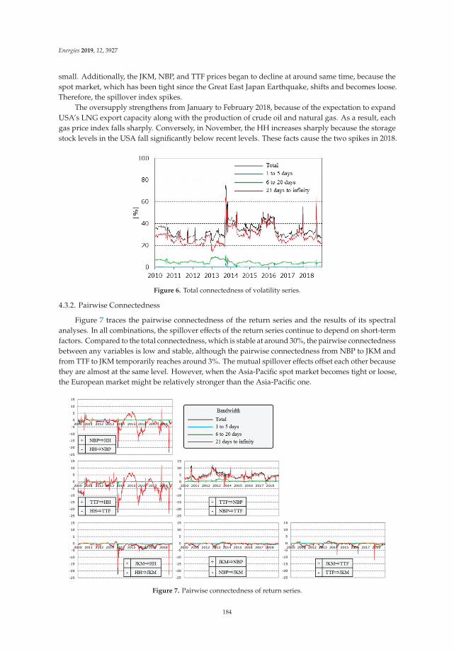
Energies 2019, 12, 3927

small. Additionally, the JKM, NBP, and TTF prices began to decline at around same time, because thespot market, which has been tight since the Great East Japan Earthquake, shifts and becomes loose.Therefore, the spillover index spikes.

The oversupply strengthens from January to February 2018, because of the expectation to expandUSA’s LNG export capacity along with the production of crude oil and natural gas. As a result, eachgas price index falls sharply. Conversely, in November, the HH increases sharply because the storagestock levels in the USA fall significantly below recent levels. These facts cause the two spikes in 2018.

Figure 6. Total connectedness of volatility series.

4.3.2. Pairwise Connectedness

Figure 7 traces the pairwise connectedness of the return series and the results of its spectralanalyses. In all combinations, the spillover effects of the return series continue to depend on short-termfactors. Compared to the total connectedness, which is stable at around 30%, the pairwise connectednessbetween any variables is low and stable, although the pairwise connectedness from NBP to JKM andfrom TTF to JKM temporarily reaches around 3%. The mutual spillover effects offset each other becausethey are almost at the same level. However, when the Asia-Pacific spot market becomes tight or loose,the European market might be relatively stronger than the Asia-Pacific one.

Figure 7. Pairwise connectedness of return series.

184

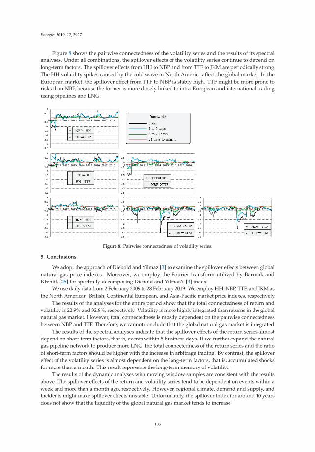
Energies 2019, 12, 3927

Figure 8 shows the pairwise connectedness of the volatility series and the results of its spectralanalyses. Under all combinations, the spillover effects of the volatility series continue to depend onlong-term factors. The spillover effects from HH to NBP and from TTF to JKM are periodically strong.The HH volatility spikes caused by the cold wave in North America affect the global market. In theEuropean market, the spillover effect from TTF to NBP is stably high. TTF might be more prone torisks than NBP, because the former is more closely linked to intra-European and international tradingusing pipelines and LNG.

Figure 8. Pairwise connectedness of volatility series.

5. Conclusions

We adopt the approach of Diebold and Yilmaz [3] to examine the spillover effects between globalnatural gas price indexes. Moreover, we employ the Fourier transform utilized by Baruník andKrehlík [25] for spectrally decomposing Diebold and Yilmaz’s [3] index.

We use daily data from 2 February 2009 to 28 February 2019. We employ HH, NBP, TTF, and JKM asthe North American, British, Continental European, and Asia-Pacific market price indexes, respectively.

The results of the analyses for the entire period show that the total connectedness of return andvolatility is 22.9% and 32.8%, respectively. Volatility is more highly integrated than returns in the globalnatural gas market. However, total connectedness is mostly dependent on the pairwise connectednessbetween NBP and TTF. Therefore, we cannot conclude that the global natural gas market is integrated.

The results of the spectral analyses indicate that the spillover effects of the return series almostdepend on short-term factors, that is, events within 5 business days. If we further expand the naturalgas pipeline network to produce more LNG, the total connectedness of the return series and the ratioof short-term factors should be higher with the increase in arbitrage trading. By contrast, the spillovereffect of the volatility series is almost dependent on the long-term factors, that is, accumulated shocksfor more than a month. This result represents the long-term memory of volatility.

The results of the dynamic analyses with moving window samples are consistent with the resultsabove. The spillover effects of the return and volatility series tend to be dependent on events within aweek and more than a month ago, respectively. However, regional climate, demand and supply, andincidents might make spillover effects unstable. Unfortunately, the spillover index for around 10 yearsdoes not show that the liquidity of the global natural gas market tends to increase.

185

Energies 2019, 12, 3927

For practitioners, this study implies that constantly monitoring market spillovers is significant.The information obtained by this study’s approach is also of high value for energy portfolio rebalancing,including derivatives. Moreover, if we monitor the index as a predictive indicator, the informationhelps with early risk aversion.

Finally, clarification of the spillover effects between the crude oil and natural gas markets will berequired for future studies, because many natural gas trading contracts still have their prices linked tocrude oil prices.

Author Contributions: Data curation, T.N.; formal analysis, Y.T.; retry analysis, T.N.; writing, T.N.; editing, T.N.;supervision, T.N.


Acknowledgments: The authors would like to thank the anonymous reviewers, whose valuable comments helpedimprove an earlier version of this paper.


References

1. BP’s Statistical Review of World Energy. Available online: https://www.bp.com/en/global/corporate/energy-economics/statistical-review-of-world-energy.html (accessed on 29 September 2019).

2. Japan Fair Trade Commission; Government of Japan. Ekika-Ten-Nen-Gas-No-Torihiki-Jittai-Ni-Kansuru-Chousa-Houkokusho (Survey on LNG Trades). 2017. Available online: https://www.jftc.go.jp/houdou/pressrelease/h29/jun/170628_1_files/170628_4.pdf (accessed on 29 September 2019).

3. Diebold, F.X.; Yilmaz, K. Better to give than to receive: Predictive directional measurement of volatilityspillovers. Int. J. Forecast. 2012, 28, 57–66. [CrossRef]

4. Kum, H.; Ocal, O.; Aslan, A. The relationship among natural gas energy consumption, capital and economicgrowth: Bootstrap-corrected causality tests from G-7 countries. Renew. Sustain. Energy Rev. 2012, 16,2361–2365. [CrossRef]

5. Das, A.; McFarlane, A.A.; Chowdhury, M. The dynamics of natural gas consumption and GDP in Bangladesh.Renew. Sustain. Energy Rev. 2013, 22, 269–274. [CrossRef]

6. Bildirici, M.E.; Bakirtas, T. The relationship among oil, natural gas and coal consumption and economicgrowth in BRICTS (Brazil, Russian, India, China, Turkey and South Africa) countries. Energy 2014, 65,134–144. [CrossRef]

7. Acaravci, A.; Ozturk, I.; Kandir, S.Y. Natural gas prices and stock prices: Evidence from EU-15 countries.Econ. Model. 2012, 29, 1646–1654. [CrossRef]

8. Nakajima, T.; Hamori, S. Testing causal relationships between wholesale electricity prices and primaryenergy prices. Energy Policy 2013, 62, 869–877. [CrossRef]

9. Atil, A.; Lahiani, A.; Nguyen, A.D. Asymmetric and nonlinear pass-through of crude oil prices to gasolineand natural gas prices. Energy Policy 2014, 65, 567–573. [CrossRef]

10. Perifanis, T.; Dagoumas, A. Price and Volatility Spillovers Between the US Crude Oil and Natural GasWholesale Markets. Energies 2018, 11, 2757. [CrossRef]

11. Tiwari, A.K.; Mukherjee, Z.; Gupta, R.; Balcilar, M. A wavelet analysis of the relationship between oil andnatural gas prices. Resour. Policy 2019, 60, 118–124. [CrossRef]

12. Xia, T.; Ji, Q.; Geng, J.B. Nonlinear dependence and information spillover between electricity and fuel sourcemarkets: New evidence from a multi-scale analysis. Physica A 2020, 537, 122298. [CrossRef]

13. Batten, J.A.; Kinateder, H.; Szilagyi, P.G.; Wagner, N.F. Time-varying energy and stock market integration inAsia. Energy Econ. 2019, 80, 777–792. [CrossRef]

14. Nakajima, T. Expectations for Statistical Arbitrage in Energy Futures Markets. J. Risk Financ. Manag. 2019,12, 14. [CrossRef]

15. Olsen, K.K.; Mjelde, J.W.; Bessler, D.A. Price formulation and the law of one price in internationally linkedmarkets: An examination of the natural gas markets in the USA and Canada. Ann. Reg. Sci. 2015, 54,117–142. [CrossRef]

186

Energies 2019, 12, 3927

16. Scarcioffolo, A.R.; Etienne, X.L. How connected are the U.S. regional natural gas markets in thepost-deregulation era? Evidence from time-varying connectedness analysis. J. Commod. Mark. 2019,15, 100076. [CrossRef]

17. Ren, X.; Lu, Z.; Cheng, C.; Shi, Y.; Shen, J. On dynamic linkages of the state natural gas markets in the USA:Evidence from an empirical spatio-temporal network quantile analysis. Energy Econ. 2019, 80, 234–245.[CrossRef]

18. Nick, S. The informational efficiency of European natural gas hubs: Price formation and intertemporalarbitrage. Energy J. 2016, 37, 1–30. [CrossRef]

19. Osicka, J.; Lehotský, L.; Zapletalová, V.; Cernoch, F.; Dancák, B. Natural gas market integration in theVisegrad 4 region: An example to follow or to avoid? Energy Policy 2018, 112, 184–197. [CrossRef]

20. Bastianin, A.; Galeotti, M.; Polo, M. Convergence of European natural gas prices. Energy Econ. 2019, 81,793–811. [CrossRef]

21. Shi, X.; Shen, Y.; Wu, Y. Energy market financialization: Empirical evidence and implications from East AsianLNG markets. Financ. Res. Lett. 2019, 30, 414–419. [CrossRef]

22. Neumann, A. World natural gas markets and trade: A multi-modeling perspective. Energy J. 2009, 30,187–199. [CrossRef]

23. Chai, J.; Wei, Z.; Hu, Y.; Su, S.; Zhang, Z.G. Is China’s natural gas market globally connected? Energy Policy2019, 132, 940–949. [CrossRef]

24. Silverstovs, B.; L’Hégaret, G.; Neumann, A.; Hirschhausen, C. International market integration for naturalgas? A cointegration analysis of prices in Europe, North America and Japan. Energy Econ. 2005, 27, 603–615.[CrossRef]

25. Baruník, J.; Krehlík, T. Measuring the frequency dynamics of financial connectedness and systemic risk.J. Financ. Econom. 2018, 16, 271–296. [CrossRef]

26. Toyoshima, Y.; Hamori, S. Measuring the time-frequency dynamics of return and volatility connectedness inglobal crude oil markets. Energies 2018, 11, 2893. [CrossRef]

27. Ji, Q.; Geng, J.B.; Tiwary, A.K. Information spillovers and connectedness networks in the oil and gas markets.Energy Econ. 2018, 75, 71–84. [CrossRef]

28. Engle, R.F.; Kroner, K.F. Multivariate Simultaneous Generalized ARCH. Econom. Theory 1995, 11, 122–150.[CrossRef]


187

MDPISt. Alban-Anlage 66

4052 BaselSwitzerland

Tel. +41 61 683 77 34Fax +41 61 302 89 18

www.mdpi.com

Energies Editorial OfficeE-mail: [email protected]

www.mdpi.com/journal/energies

MDPI St. Alban-Anlage 66 4052 Basel Switzerland

Tel: +41 61 683 77 34 Fax: +41 61 302 89 18

www.mdpi.com ISBN 978-3-03943-137-3

Empirical analysis of natural gas markets - econstor

Documents

Transcript of Empirical analysis of natural gas markets - econstor