Correlation in Energy Markets - EconStor
181
Lange, Nina Doctoral Thesis Correlation in Energy Markets PhD Series, No. 8.2017 Provided in Cooperation with: Copenhagen Business School (CBS) Suggested Citation: Lange, Nina (2017) : Correlation in Energy Markets, PhD Series, No. 8.2017, ISBN 9788793483897, Copenhagen Business School (CBS), Frederiksberg, https://hdl.handle.net/10398/9461 This Version is available at: http://hdl.handle.net/10419/209016 Standard-Nutzungsbedingungen: Die Dokumente auf EconStor dürfen zu eigenen wissenschaftlichen Zwecken und zum Privatgebrauch gespeichert und kopiert werden. Sie dürfen die Dokumente nicht für öffentliche oder kommerzielle Zwecke vervielfältigen, öffentlich ausstellen, öffentlich zugänglich machen, vertreiben oder anderweitig nutzen. Sofern die Verfasser die Dokumente unter Open-Content-Lizenzen (insbesondere CC-Lizenzen) zur Verfügung gestellt haben sollten, gelten abweichend von diesen Nutzungsbedingungen die in der dort genannten Lizenz gewährten Nutzungsrechte. Terms of use: Documents in EconStor may be saved and copied for your personal and scholarly purposes. You are not to copy documents for public or commercial purposes, to exhibit the documents publicly, to make them publicly available on the internet, or to distribute or otherwise use the documents in public. If the documents have been made available under an Open Content Licence (especially Creative Commons Licences), you may exercise further usage rights as specified in the indicated licence. https://creativecommons.org/licenses/by-nc-nd/3.0/
-
Upload
khangminh22 -
Category
Documents
-
view
0 -
download
0
Transcript of Correlation in Energy Markets - EconStor
Lange, Nina
Doctoral Thesis
Correlation in Energy Markets
PhD Series, No. 8.2017
Provided in Cooperation with:Copenhagen Business School (CBS)
Suggested Citation: Lange, Nina (2017) : Correlation in Energy Markets, PhD Series, No.8.2017, ISBN 9788793483897, Copenhagen Business School (CBS), Frederiksberg,https://hdl.handle.net/10398/9461
This Version is available at:http://hdl.handle.net/10419/209016
Standard-Nutzungsbedingungen:
Die Dokumente auf EconStor dürfen zu eigenen wissenschaftlichenZwecken und zum Privatgebrauch gespeichert und kopiert werden.
Sie dürfen die Dokumente nicht für öffentliche oder kommerzielleZwecke vervielfältigen, öffentlich ausstellen, öffentlich zugänglichmachen, vertreiben oder anderweitig nutzen.
Sofern die Verfasser die Dokumente unter Open-Content-Lizenzen(insbesondere CC-Lizenzen) zur Verfügung gestellt haben sollten,gelten abweichend von diesen Nutzungsbedingungen die in der dortgenannten Lizenz gewährten Nutzungsrechte.
Terms of use:
Documents in EconStor may be saved and copied for yourpersonal and scholarly purposes.
You are not to copy documents for public or commercialpurposes, to exhibit the documents publicly, to make thempublicly available on the internet, or to distribute or otherwiseuse the documents in public.
If the documents have been made available under an OpenContent Licence (especially Creative Commons Licences), youmay exercise further usage rights as specified in the indicatedlicence.
https://creativecommons.org/licenses/by-nc-nd/3.0/

Nina Lange
The PhD School in Economics and Management PhD Series 08.2017
PhD Series 08-2017CORRELATION
IN EN
ERGY MARKETS
COPENHAGEN BUSINESS SCHOOLSOLBJERG PLADS 3DK-2000 FREDERIKSBERGDANMARK
WWW.CBS.DK
ISSN 0906-6934
Print ISBN: 978-87-93483-88-0Online ISBN: 978-87-93483-89-7
CORRELATION IN ENERGY MARKETS
Correlation in Energy Markets
Nina Lange
Submitted: August 31, 2016
Academic advisor: Carsten Sørensen
The PhD School in Economics and Management
Copenhagen Business School

Nina LangeCorrelation in Energy Markets
1st edition 2017PhD Series 08.2017
© Nina Lange
ISSN 0906-6934
Print ISBN: 978-87-93483-88-0 Online ISBN: 978-87-93483-89-7
“The PhD School in Economics and Management is an active national and international research environment at CBS for research degree studentswho deal with economics and management at business, industry and countrylevel in a theoretical and empirical manner”.
All rights reserved.No parts of this book may be reproduced or transmitted in any form or by any means,electronic or mechanical, including photocopying, recording, or by any informationstorage or retrieval system, without permission in writing from the publisher.

Preface
Preface
This dissertation concludes my years as an Industrial PhD student at Department of
Finance, Copenhagen Business School and Customers & Markets, DONG Energy A/S. The
dissertation consists of four essays within the overall topic of energy markets. Although the
last three essays are on the same topic, all four essays are self-contained and can be read
independently of each other. Essay I studies the relationship of volatility in oil prices and
the EURUSD rate and how it has evolved over time. Essay II-IV are on the so-called energy
quanto options – a contract paying the product of two options. Essay II shows why energy
quanto options are strong candidates for Over-The-Counter structured hedge strategies.
Essay III (co-authored with Fred Espen Benth and Tor Åge Myklebust) studies the pricing
of energy quanto option in a log-normal framework and Essay IV presents an approximation
formula for the price of an energy quanto option using Greeks, individual option prices and
the correlation among assets.
Publication details
The third essay is published in Journal of Energy Markets (2015), Volume 8, no. 1, p. 1-35.
Acknowledgements
First, thanks to my advisor, Carsten Sørensen, for encouragement and for providing me
with an overview all the times I lost it. Secondly, thanks to DONG Energy and the business
unit Customers & Markets for collaborating on this Industrial PhD. I am grateful to Sune
Korreman for hiring me many years back and supporting my shift to research, to Peter Lyk-
Jensen for being a calm and supporting company advisor, to Lars Bruun Sørensen for initial
financial support of the PhD project and to Per Tidlund for doing his best to include me
in the department on a daily basis. Also thanks to my (former) colleagues in Quantitative
i

Preface
Analytics. It has been a pleasure discussing both research and non-research topics with all
of you.
I am beyond grateful for my collaboration with Fred Espen Benth at the University of Oslo.
It has been a privilege to work with such an experienced and structured researcher and I
look forward to continue on the projects in our joint pipeline. The time spend lecturing,
examining and supervising jointly with Kristian Miltersen within the field of energy markets
provided me with a good foundation for my future teaching activities. During my second
year, I had the opportunity to visit Andrea Roncoroni at ESSEC Business School in Paris
and Singapore. I learned a lot from this visit. During my last year at CBS, I was funded
by CBS Maritime. The inclusion in CBS Maritime and cooperation on teaching shipping
related topics was a great experience and I hope to pursue this topic also as a research area.
I appreciate the comments from the Committee of my closing seminar on April 29, 2016;
Anders Trolle and Bjarne Astrup Jensen, and especially thanks to Bjarne for pointing out
literature related to Essay II.
A big thanks to René Kallestrup for the introduction to Bloomberg and to Mads Stenbo
Nielsen, David Skovmand, Desi Volker and Michael Coulon for endless discussions about
life and life as a researcher.
Last, but not least, Martin; thank you for always being there even when I was impossible.
Nina Lange
Frederiksberg, August 31 2016
ii

Summary
Summary
English Summary
Essay I: Volatility Relations in Crude Oil Prices and the EURUSD rate
In this paper, I study the relationship between volatility of crude oil prices and volatility of
the EURUSD rate. If there is a common factor in the volatility of crude oil and the volatility
of exchange rates, possible explanations could be that the financial crisis caused a volatility
spillover between the two markets or that commodity markets, one of the most important
being the crude oil market, are strengthening their connection with classic financial markets
including exchange rate markets.
I use an extensive data set of crude oil futures and options and EURUSD futures and
options spanning a period from 2000 to 2012. This data allows me to analyse the market-
perceived volatility rather than investigating volatilities in the form of realised returns.
A model-free analysis supports the presence of a joint factor in the volatilities since
mid-2007. As the two markets are asynchronous in futures and options maturity date, a
term structure models allow for a description of the observed volatility surfaces by one or
more stochastic volatility processes. A term structure model including one joint volatility
factor and two market-specific volatility factors is proposed to capture the joint factor in
the volatilities from 2007 onwards.
The paper focuses on confirming the existence of a joint factor, but leaves out the
explanation of where it comes from. As data only covers until 2012, there is not enough
information post-crisis to distinguish whether the joint volatility is a financialization or a
crisis effect – or a combination.
iii
Summary
Essay II: How Energy Quanto Options can Hedge Volumetric Risk
In this paper, the performance of energy quanto options as a tool for hedging volumetric
risk is compared to other proposed hedge strategies. Volumetric risk is defined as the
impact of fluctuations in demand on revenue and is not a unique problem for commodity
markets. The difference between commodity markets and other markets is however that
in commodity markets, market participants has little or no control over the demanded
or supplied quantity and corresponding prices. For instance in liberalised energy markets,
standard contract structures require energy companies to deliver any amount of energy
demanded by the customers at a pre-determined price. The significant positive relationship
between demanded quantity and associated market prices makes this contract structure
risky for energy companies. When prices are low and they face a positive profit margin on
the energy they sell, they sell a relatively small amount. On the other hand, when prices are
high and the profit margin is negative, the customer demands a relatively larger quantity,
which leads to a loss for the energy company. The lack of control over market prices as well
as the sold volume give companies reasons for employing hedge strategies using the financial
markets, either in form exchange traded derivatives or OTC-traded derivatives.
Proposed strategies include forward or futures and options written on the underlying
energy price. The exact choice of contracts is impacted by the correlation between quantity
and prices. A natural extension of these hedging strategies is to include derivatives on
weather, as weather and quantity for many cases show significant correlation. Other
strategies do not specifically define the derivative type used in the hedge strategy, but
derives the hedge as a general function of price. This idea is extended to a hedging strategy
depending not only on the price, but also an index, e.g., weather, related to the quantity. The
general expression for the hedge is in simple cases obtainable in closed form, but nevertheless
it does not have a structure that appeals to an OTC counterpart.
Mathematically, the general hedge strategy written on both price and index can be
replicated using, among other, energy quanto options, e.g., options which pays out a product
of two standard options. These structures are offered by re-insurance companies and used by
energy companies as a way to hedge against an adverse situation, where the energy company
risk low revenues. Using a comparative study, the performance of energy quanto options is
proved to do almost as well as the optimal hedge. As the optimal hedge is infeasible to obtain
in the OTC market, the energy quanto option is a strong candidate for risk management.
iv

Summary
The energy quanto strategy also outperforms any other strategy consisting of market traded
contracts. Further, the study illustrates that the exact choice of energy quanto options
depends on the behaviour of the underlying variables.
Essay III: Pricing and Hedging Energy Quanto Options
In this paper, we study the pricing and hedging energy quanto options. Energy quanto
options are tools to manage the joint exposure to weather and price variability. An example
is a gas distribution company that operates in an open wholesale market. If, for example,
one of the winter months turns out to be warmer than usual, the demand for gas would
drop. This decline in demand would probably also affect the market price for gas, leading
to a drop in gas price. The firm would make a loss compared with their planned revenue
through not only the lower demand also through the indirect effect from the drop in market
prices.
Since 2008, the market for standardized contracts has experienced severe retrenchment
and a big part of this sharp decline is attributed to the substantial increase in the market
for tailor-made contracts. As these tailor-made energy quanto options are often written on
the average of price and the average weather index, we convert the pricing problem by using
traded futures contracts on energy and a temperature index as underlying assets, as these
settle to the average of the spot.
We derive options prices under the assumption that futures prices are log-normally
distributed. Using futures contracts on natural gas and the Heating Degree Days (HDDs)
temperature index, we estimate a model based on data collected from the New York
Mercantile Exchange and the Chicago Mercantile Exchange. We compute prices for various
energy quanto options and benchmark these against products of plain-vanilla European
options on gas and HDD futures.
Essay IV: A Short Note on Pricing of Energy Quanto Options
In this short note, an approximation for the price of an energy quanto option is proposed. An
energy quanto option is an option written on the price of energy and a quantity related index,
for instance weather. The option only pays off if both prices and the weather index are in
the money and such structures are useful to hedge volumetric risk in energy markets. Under
the assumption of a log-normal prices, the energy quanto option price can be approximated
v

Summary
by a pricing formula involving the correlation, current individual asset prices and option
prices, volatilities and Greeks. These quantities are known or can be assessed by market
participants, thereby yielding a fast pricing method for energy quanto options. The pricing
performance is illustrated using a simple numerical example.
vi
Summary
Dansk Resumé
Essay I: Sammenhæng mellem olieprisers og valutakursers volatilitet
I denne artikel undersøger jeg sammenhængen mellem volatiliteten af oliepriser og EURUSD
kursen. Hvis en fælles faktor driver volatiliteten i både oliepriser og valutakurser, kunne en
mulig forklaring være at finanskrisen er skyld i at volatilitet fra det ene market flyder
over til det andet market. En anden forklaring kunne være at råvaremarkeder, hvoraf et
af de vigtigste er oliemarkedet, har fået styrket deres forbindelse til de klassiske finansielle
markeder, herunder valutamarkederne.
Jeg bruger et omfangsrigt datasæt bestående af priser på oliefutures og -optioner samt
EURUSD-futures og -optioner fra perioden 2000-2012. Dette datasæt giver mig mulighed
for at analysere den markedsimplicitte volatilitet fremfor realiseret volatilitet udledt fra
spotpriser.
En modelfri analyse understøtter eksistensen af en fælles faktor i volatiliteterne siden
midten af 2007. De to markeders futures og optioner har ikke samme udløbstidspunkter,
så jeg opstiller en model som kan sammenkoge hele volatilitetsoverfladen til en eller
flere stokastiske volatilitetsprocesser. En model med en fælles volatilitetsproces og to
markedsspecifikke volatilitetsprocesser foreslås og estimeres for at fange den fælles faktor i
volatiliteter siden 2007.
Artiklen fokuserer på at bekræfte eksistensen af den fælles faktor, men omhandler ikke
en forklaring på hvorfra den kommer. Da datasættet kun dækker perioden frem til 2012,
er der ikke nok post-krise data til at identificere, om den fælles volatilitet kommer fra
finansialisering af råvaremarkederne eller fra finanskrisen – eller en kombination.
Essay II: Double-trigger optioners evne til at hedge volumenrisiko i energimarkeder
I denne artikel sammenlignes det hvordan double-trigger optioner på priser og mængder
klarer sig sammenlignet med andre hedgestrategier, når det drejer sig om at at styre
volumenrisiko. Volumenrisiko er defineret som indvirkningen på omsætningen som følge af
fluktuationer i efterspørgsel og findes ikke kun på råvaremarkeder. Forskellen er imidlertid
at markedsdeltagerne i råvaremarkeder har lille eller ingen kontrol over efterspurgt eller
produceret mængde og dertilhørende priser. For eksempel, på det liberaliserede elmarked vil
en almindelig kontraktstruktur forpligte forsyningsselskabet til at levere en hvilken som helst
vii

Summary
efterspurgt mængde af strøm til en på forhånd fastsat pris. Den klart positive relation mellem
efterpsurgt mændge og tilhørende markedspriser gør denne kontraktstruktur risikabel for
forsyningsselskabet. Når priserne er lave og deres profitmargin er positiv, sælger de relativt
lidt. Omvendt, når priserne er høje og profitmarginen er negativ, efterspørger kunden en
relativt større mængde, hvilket resulterer i et tab. Manglen på kontrol over priser såvel
som mængder giver virksomheder god grund til at anvende hedgestrategier indeholdende
derivater, enten ved hjælp af standardiserede kontrakter eller gennem en direkte modpart.
Foreslåede strategier inkluderer forwards eller futures og optioner skrevet på energiprisen.
Det præcise valg af kontrakter er afhængig af korrelationen mellem pris og mængde. En
naturlig udvidelse af dette er at inkludere derivater som afhænger af vejr, da vejr og
mængde i mange tilfælde udviser en signifikant korrelation. Andre strategier specificerer
ikke den præcise type af derivat, men udleder hedgestrategien som en generel funktion af
energiprisen. Denne ide kan udvides til en hedgestrategi, som ikke kun afhænger af pris, men
også et index, fx. vejr, som relaterer sig til mængde. I simple tilfælde er kan dette hedge
udtrykkes i lukket form, men dets struktur vil på ingen måde appelere til en modpart.
Matematisk kan den generelle hedgestrategi skrevet på både energipris og index replikeres
ved hjæpl af blandt andet double-trigger optioner, dvs. optioner der betaler et produkt af
to almindelige optioner. Sådanne strukturer tilbydes for eksempel af genforsikringsselskaber
og bruges af energiselskaber som en måde at sikre sig mod en situation hvor omsætningen
er kritisk lav.
En sammenligning viser at double-trigger optioner skrevet på pris og et vejrindex klarer
sig stort set lige så godt som det optimale teoretiske hedge. Da det optimale teoretiske
hedge ikke er muligt at opnå i praksis, er double-trigger optioner potentielt en stærk
kandidat til en risikostyringsstrategi. Ydermere klarer double-trigger optionerne sig bedre
end markedsbaserede stratgier. Endeligt viser eksemplet at det præcise valg af double-trigger
optioner er afhængig af fordelingen af de underliggende variable.
Essay III: Prisfastsættelse og hedging af dobbelt-trigger optioner på energi og
mængder
I denne artikel studerer vi prisfastsættelse af dobbelt-trigger optioner på energi og mængder.
Dobbelt-trigger optioner på energi og mængder er redskaber til at styre den fælles
eksponering mod vejr og prisusikkerheder. Et eksempel er et gasdistributionsselskab, som
viii
Summary
opererer i engrosmarkedet. Hvis, for eksempel, en vintermåned er varmere end normalt vil
efterspørgslen efter gas falde. Dette fald i efterspørgsel vil også påvirke markedsprisen for
gas i nedadgående retning. Gasdistributionsselskabet vil derfor have et tab sammenlignet
med deres budgetterede omsætning og dette tab kommer både fra det lavere salg, men også
indirekte fra faldet i priser.
Siden 2008 er markedet for standardiserede vejrkontrakter blevet betydeligt mindre og
en stor del af dette fald skyldes den betydelige stigning i markedet for skræddersyede
kontrakter på vejr. Eftersom disse skræddersyede kontrakter ofte er skrevet på et gennemsnit
af priser og et gennemsnit af et vejrindex og da futureskontrakter ligeledes afregnes mod en
gennemsnit af prisen over en periode, omskriver vi prisfastsættelsesproblemet ved at bruge
futureskontrakter på energi og vejr som underliggende kontrakter.
Vi udleder optionspriser under en antagelse om at futurespriser er log-normalfordelte.
For futureskontrakter på gas og på temperaturindekset Heating Degree Days (HDDs),
estimerer vi en model baseret på data fra New York Mercantile Exchange og Chicago
Mercantile Exchange. Vi udregner priser for diverse dobbelt-trigger optioner på gas og
temperaturindexet og benchmarker disse mod produktet af standard optioner på gas og
standard optioner på temperaturindexet.
Essay IV: En kort bemærkning om prisfastsættelse af dobbelt-trigger optioner
I denne korte note præsenteres en approksimation for prisen for en dobbelt-trigger optioner
på energi og mængder. En dobbelt-trigger option er et derivat skrevet på prisen af
energi og en mængderelateret indeks, for eksempel vejr. Optionen betaler kun, hvis både
prisen påenergi og vejrindekset er ”i pengene” og sådanne strukturer er nyttige for at
styre volumenrisiko på energimarkederne. Under antagelse af log-normalfordelte priser,
kan dobbelt-trigger optionen approximeres af en prisformel, der involverer korrelation,
individuelle underliggende priser og optionspriser, volatiliteter og Greeks. Alle disse
størrrelser er kendte eller kan blive tilnærmet af markedsdeltagerne og dermed kan dobbelt-
trigger optioner nemt og hurtigt prisfastsættes. Nøjagtigheden af formlen er illustreret i et
simpelt numerisk eksempel.
ix

Contents
Contents
Preface i
Summary iii
English Summary . . . . . . . . . . . . . . . . . . . . . . . . . . . iii
Dansk Resumé. . . . . . . . . . . . . . . . . . . . . . . . . . . . . vii
Introduction 1
Essay I Volatility Relations in Crude Oil Prices and the EURUSD rate 5
I.1 Introduction . . . . . . . . . . . . . . . . . . . . . . . . . . . 6
I.2 Overview of data . . . . . . . . . . . . . . . . . . . . . . . . . 8
I.3 Model-free Analysis: Joint Volatility Factors . . . . . . . . . . . . . . 15
I.4 A Linked Model for Derivatives on Oil and the EURUSD . . . . . . . . . 22
I.5 Results . . . . . . . . . . . . . . . . . . . . . . . . . . . . . 26
I.6 Conclusion . . . . . . . . . . . . . . . . . . . . . . . . . . . . 40
I.A Data Description . . . . . . . . . . . . . . . . . . . . . . . . . 41
I.B Kalman Filter . . . . . . . . . . . . . . . . . . . . . . . . . . 49
Essay II How Energy Quanto Options can Hedge Volumetric Risk 53
II.1 Introduction . . . . . . . . . . . . . . . . . . . . . . . . . . . 54
II.2 Background and related literature. . . . . . . . . . . . . . . . . . . 56
xi
Contents
II.3 Risk management problem for an energy retailer . . . . . . . . . . . . . 60
II.4 Comparative study . . . . . . . . . . . . . . . . . . . . . . . . 63
II.5 Concluding remarks . . . . . . . . . . . . . . . . . . . . . . . . 77
II.A Details of benchmark strategies. . . . . . . . . . . . . . . . . . . . 78
Essay III Pricing and Hedging Energy Quanto Options 85
III.1 Introduction . . . . . . . . . . . . . . . . . . . . . . . . . . . 86
III.2 The contract structure and pricing of energy quanto options . . . . . . . . 89
III.3 Asset Price Dynamics and Option Prices . . . . . . . . . . . . . . . . 94
III.4 Empirical Analysis. . . . . . . . . . . . . . . . . . . . . . . . . 100
III.5 Concluding remarks . . . . . . . . . . . . . . . . . . . . . . . . 107
III.A Proof of pricing formula . . . . . . . . . . . . . . . . . . . . . . 110
III.B Closed-form solution for σ and ρ in the two-dimensional Schwartz-Smith model
with seasonality . . . . . . . . . . . . . . . . . . . . . . . . . . 113
III.C One-dimensional option prices . . . . . . . . . . . . . . . . . . . . 114
III.D Estimation using Kalman filter techniques . . . . . . . . . . . . . . . 114
III.E Result of analysis using data from Chicago . . . . . . . . . . . . . . . 116
Essay IV A Short Note on Pricing of Energy Quanto Options 121
IV.1 Introduction . . . . . . . . . . . . . . . . . . . . . . . . . . . 122
IV.2 The Quick and Dirty Formulas . . . . . . . . . . . . . . . . . . . . 122
IV.3 Numerical Example . . . . . . . . . . . . . . . . . . . . . . . . 124
IV.4 Concluding remarks . . . . . . . . . . . . . . . . . . . . . . . . 125
IV.A Proof of propositions IV.1-IV.2 . . . . . . . . . . . . . . . . . . . . 127
IV.B Delta and Gamma expressions . . . . . . . . . . . . . . . . . . . . 128
Conclusion 133
Bibliography 135
xii
Introduction
Introduction
In the recent years, the size of commodity derivatives markets have increased. The U.S.
Energy Information Administration reports that the number of outstanding WTI crude
oil futures on U.S. exchanges has more than quadrupled from 2000 to 2016. The market
participant can be both hedgers such as producers and end-users or speculators, who have
no interest in the underlying oil as a commodity. Besides the general links of commodity
prices and the world economy and the world economy and financial markets, the presence
of financial investors in commodity market is a direct link between commodities markets
and regular financial markets.
In commodity markets, spot prices are a result of supply and demand in a given location.
Surrounding the physical market is a huge commodity derivatives markets, where prices of
futures, forwards, swaps and options are related to the spot prices either because physical
delivery is possible of because the contract is settled to underlying spot prices. The link
between spot prices and the derivatives market differ from market to market. The exact
relationship between the spot and derivatives market on commodities suck as oil is explained
by the concept of convenience yields, which is a benefit or a cost accruing to the holder of
the commodity, but not to the owner of a forward or futures on the commodity. Using
this theory, the difference in spot prices today compared to the price of a oil futures is
explained by storage costs, funding costs and potential non-monetary benefits of possessing
the physical commodity between today and maturity. The convenience yield or equivalently
the shape of the futures curve behaves dynamically as a reflection to the spot and financial
markets. Over the past years, the oil futures curve has been in contango (oil futures with
longer maturities are more expensive), in backwardation (oil futures with longer maturities
are less expensive) or shown a hump-structure. While it must be expected that spot prices
are solely driven by fundamentals, the question of whether the futures prices are driven by
fundamentals or by financial investors has attracted much attention over the last decade.
1
Introduction
Starting in 2004, commodity markets saw a general increase in prices, in volatility
and in co-movement with other asset classes. One string of literature argues that this is
due to financialization of commodity markets – a term used to describe increased role of
financial investors. This theory states that the changes in markets is caused by the inflow of
investments into commodity markets from large investors, see e.g., Tang and Xiong (2012) or
Carmona (2015). Contradicting this theory is e.g., Kilian (2009) who argues that the change
in commodity markets are driven by fundamentals, while others seek a compromise between
the two theories as for instance Vansteenkiste (2011), who claims that both investors and
fundamentals play a role in price determination with the former domination the majority
of the time during the last decade. Similar conclusions are drawn by Basak and Pavlova
(2016) who estimate that around 15% of the futures price comes from financialization and
the rest from fundamentals.
Essay I in this dissertation is related to the intersection of commodity and financial
markets. It considers the oil market and a foreign exchange market. These two markets
are often analysed in terms of correlation between spot returns and the results depend on
whether the currency in question is from a country with a large export of commodities. In
my analysis, I focus specifically on the EURUSD rate. None of the countries in the Euro-
zone are considered major commodity exporters, so the EURUSD rate and crude oil price
will largely be expected to have a positive correlation when looking a returns or levels, the
argument being that as the Dollar depreciates against the Euro (meaning the EURUSD rate
increases), the oil-importing Euro-zone will import more and thereby increase oil prices. The
relationship is especially strong just before the financial crisis (see Verleger (2008)). How
volatilities in these two markets relate is a less studied question. Ding and Vo (2012) find
that for realized volatility of spot oil prices and spot EURUSD rates, there are indications
of volatility spillovers from one market to another after the financial crisis started. In my
analysis, I use options on futures and using first a model-free approach, I find that there is a
joint volatility factor for the two markets after 2007. I then propose a term structure model
along the lines of Trolle and Schwartz (2009) for future and options and estimate this model.
After 2007, adding a joint volatility factor to explain the co-movement in volatilities in the
two markets gives a better fit to the observed implied volatility surfaces. The improvement
in the volatility fit is highly significant for the oil options and for shorter EURUSD options.
Whether the presence of a joint factor is a result of fundamentals, financialization or the
financial crisis is left for later studies.
2
Introduction
The remaining part of this dissertation it devoted to the study of volumetric risk.
Volumetric risk is defined as the impact on revenue from fluctuations in demand. Compared
to other markets, market participants in commodity markets has less over the demanded
or supplied quantity and corresponding prices. For instance in liberalised energy markets,
standard contract structures require energy companies to deliver any amount of energy
demanded by the customers at a pre-determined rate. The significant positive relationship
between demanded quantity and associated market prices makes this contract structure
risky for energy companies. When prices are low and they face a positive profit margin on
the energy they sell, they sell a relatively smaller amount. On the other hand, when prices
are high and the profit margin is negative, the customer demands a relatively larger quantity
resulting in a loss for the energy company. Another example is the owner of a wind park
producing power in a competitive electricity market. The wind speed and direction solely
determines the quantity produced and the market determines the prices, leaving the owner
as both price taker and quantity taker.
First, Essay II shows why energy quanto options1 arise when hedging the volumetric
risk. The name energy quanto option is used for a derivative paying the product of two
options. This type of derivative arises from deriving an optimal theoretical hedge strategy
based on both the underlying price and a quantity-related and market-traded index, for
instance weather. Using a numerical experiment, it is shown that in comparison with
the optimal theoretical hedge, energy quanto options are strong candidates for Over-The-
Counter structured hedge strategies. By just using one or two quanto options, the hedge
performance is 90-98% compared to the preferred theoretical hedge. Further, the energy
quanto hedge is superior in the sense, that it has an understandable structure. The optimal
theoretical hedge is in best case expressed by conditional profit expectations and density
ratios and therefore not a contract structure to request from an OTC counterpart. While
the use of an OTC counterpart rather than a market traded hedge might seem as a big step
to take for an energy company, it further has the benefit of being able to choose the exact
weather index which correlates well with the risk taken by the company rather than having
to rely on available weather contracts.
Essay III (co-authored with Fred Espen Benth and Tor Åge Myklebust) studies the
pricing of the aforementioned energy quanto options is a log-normal framework. In practice,
1Other common names are double trigger options or cross-commodity-weather options.
3

Introduction
an energy quanto option is an Asian type option written on the average of a price or an
index, and we therefore convert the pricing problem by arguing that writing an option on
an average is essentially the same as writing it on a futures contract settling on the average
price or index during the same period. With futures contracts being traded assets, we can
extract the pricing measure from market data and use this to provide pricing and hedging
formulas for energy quanto options. In a log-normal framework, both the price and Greeks
are available in closed form. We estimate a model for US NYMEX gas futures and Heating
Degree Days futures for New York and Chicago based on the model by Sørensen (2002).
We use the estimated model to illustrate the difference of energy quanto option prices and
plain vanilla options.
Essay IV provides a pricing approximation formula for energy quanto options. Using
a Taylor-expansion around the correlation of prices, it is shown that a first order
approximation can be obtained from univariate option prices and Deltas. A second order
approximation is obtained by adding Gammas. Many traders will have either information
or an educated guess for these quantities, making the pricing formula easy to use. If market
prices and Greeks are available, it becomes (approximately) redundant to estimate the model
as all information is already incorporated in prices and Greeks. Using a simple example, the
second order approximation is shown to be close to the actual price.
4
Volatility Relations in Crude Oil Prices and the EURUSD rate
Essay I
Volatility Relations in Crude Oil Prices and the
EURUSD rate∗
Abstract
Studies on the relationship between oil prices and the EURUSD rate is mostly
focused on the correlation of returns or levels. However, the volatility of oil price
and the volatility of the EURUSD rate is also of importance for e.g., portfolio risk
management, margin requirements or derivatives pricing models. In this paper, the
relationship between the volatility of crude oil and the volatility of the EURUSD
rate is analysed. A model-free analysis shows the presence of a joint factor in
the volatilities after mid-2007. A term structure model for futures and options on
both oil and EURUSD is proposed and estimated to WTI Crude Oil and EURUSD
futures and options traded at the Chicago Mercantile Exchange from 2000-2012.
The addition of a joint volatility factor significantly improves the fit to oil options
and short term EURUSD options after mid-2007.
∗I thank Carsten Sørensen, participants in the Bachelier World Finance Congress 2016, the Conference on the
Mathematics of Energy Markets 2016 at the Wolfgang Pauli Institute and the Energy Finance Christmas Workshop
2014 for helpful comments.
5

I.1. Introduction
I.1 Introduction
The relationship of oil prices and the EURUSD1 rate is often investigated in terms of returns
or levels. The majority of studies confirms empirically that oil and EURUSD returns or levels
are positively correlated. This implies that for a EUR-denominated investor, an increase in
oil prices is dampened by the weaker dollar and vice versa. One explanation is that a
depreciation of the US Dollar will allow a EUR-denominated investor to buy more oil for
the same amount of EUR, thereby putting an upward pressure on the oil price.
In addition to studying the size of the correlation of oil returns and EURUSD returns
(or levels), or more generally speaking foreign exchange rates, most research focuses on
the causality and forecasting performance. For instance, Chen and Chen (2007) concludes
that real oil prices have significant forecasting power when in comes to explaining real
exchange returns2. Similar conclusions are drawn by Lizardo and Mollick (2010). Research
supporting the link from currencies to commodities focuses on the so-called commodity
currencies, which are defined as currencies of countries with a large export of commodities,
e.g., Canadian Dollars, Australian Dollars or South African Rand. For instance, Chen et al.
(2010) find that commodity currencies have large predictive power for commodity prices.
Fratzscher et al. (2014) find a bidirectional causality between oil prices and the value of the
Dollar.
While there has been considerable attention on the direction of the relationship and the
possible explanations, the relationship between volatilities of the two markets have received
less attention. Ding and Vo (2012) uses a multivariate stochastic volatility framework
to investigate the volatility interaction between the oil market and the foreign exchange
markets. Using spot price data, their analysis is using realized volatility and focuses on
forecasting. They conclude that volatility spills over from one market to the other in times of
turbulence. They attributes the volatility interaction to inefficient information incorporation
during the financial crisis. The study includes only the beginning of the financial crisis, and
it is therefore not possible to determined if this only occurs during the crisis or if it is a
more permanent change.
Christoffersen et al. (2014) investigates the factor structures among different commodities
and their relation to the stock market. Using a model-free approach and high-frequency data,
1The EURUSD rate is defined as the price of euros measured in US Dollars2They do not consider the EUR, but include Germany in their analysis.
6
Volatility Relations in Crude Oil Prices and the EURUSD rate
they find that the commodity market volatilities have a strong common factor, that is largely
driven by stock market volatility. As numerous studies empirically document the relationship
between foreign exchange market volatility and stock market volatility, a natural hypothesis
is therefore a relationship between the volatility of oil and the volatility of the EURUSD.
Generally, commodity markets have seen increases in prices, volatilities and correlation
among commodities and financial assets during the last decade. One string of literature
refer to these changes as the financialization of commodity markets and explain them by the
entry of institutional investors into commodity markets, see e.g., Tang and Xiong (2012) and
Carmona (2015). Other papers, such as Kilian (2009), argue that the increase in volatilities
and in prices are solely due to fundamentals, e.g., increased demand from BRIC-countries.
In this paper, I analyse the behaviour of oil price volatility and the EURUSD volatility
to find the relationship between those and if this relationship is changing over time. The
analysis is based on exchange traded futures and options on futures. The spot price of oil is
based on actual physical trades, whereas futures on oil are mainly traded financially3. The
use of the futures market allows for viewing the volatilities as market-perceived. The use
of spot oil prices as in Ding and Vo (2012) includes potential short term impact from the
physical market rather than the volatility being seen as a reflection of the financial market.
The analysis of the volatility relation is done in two ways. First, using a model-free
approach, at-the-money straddles (written on nearby futures) with maturities up to six
months are computed for both oil and for EURUSD. The rolling correlation of short maturity
straddles is then analysed for structural breaks. The resulting sub-samples are then analysed
separately, to see if the variations in the combined straddle returns are impacted by a
common factor. Based on these results, a term structure model for pricing futures and
options is proposed and estimated. Both of these analyses show presence of a common joint
volatility factor after mid-2007.
Term structure models are well-studied in the literature. Several papers deals with
modelling of oil prices. Studies by Cortazar and Naranjo (2006), Trolle and Schwartz (2009),
Chiarella et al. (2013) all present a joint model for the term structure of futures prices and
option prices. Also FX rates and options has been widely studied, e.g., in Bakshi et al.
(2008). The model analysed in this paper is a two-asset variation of Trolle and Schwartz
3Although oil futures on WTI crude oil can be physically settled, the majority of contracts are rolled over before
maturity and thus never actually physically delivered, see e.g., the discussion about market volume and open interest
in Trolle and Schwartz (2009).
7
I.2. Overview of data
(2009).
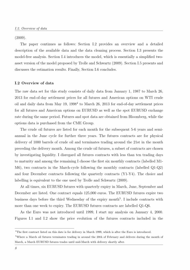
The paper continues as follows: Section I.2 provides an overview and a detailed
description of the available data and the data cleaning process. Section I.3 presents the
model-free analysis. Section I.4 introduces the model, which is essentially a simplified two-
asset version of the model proposed by Trolle and Schwartz (2009). Section I.5 presents and
discusses the estimation results. Finally, Section I.6 concludes.
I.2 Overview of data
The raw data set for this study consists of daily data from January 1, 1987 to March 26,
2013 for end-of-day settlement prices for all futures and American options on WTI crude
oil and daily data from May 19, 19984 to March 26, 2013 for end-of-day settlement prices
for all futures and American options on EURUSD as well as the spot EURUSD exchange
rate during the same period. Futures and spot data are obtained from Bloomberg, while the
options data is purchased from the CME Group.
The crude oil futures are listed for each month for the subsequent 5-6 years and semi-
annual in the June cycle for further three years. The futures contracts are for physical
delivery of 1000 barrels of crude oil and terminates trading around the 21st in the month
preceding the delivery month. Among the crude oil futures, a subset of contracts are chosen
by investigating liquidity. I disregard all futures contracts with less than ten trading days
to maturity and among the remaining I choose the first six monthly contracts (labelled M1-
M6), two contracts in the March-cycle following the monthly contracts (labelled Q1-Q2)
and four December contracts following the quarterly contracts (Y1-Y4). The choice and
labelling is equivalent to the one used by Trolle and Schwartz (2009).
At all times, six EURUSD futures with quarterly expiry in March, June, September and
December are listed. One contract equals 125,000 euros. The EURUSD futures expire two
business days before the third Wednesday of the expiry month5. I include contracts with
more than one week to expiry. The EURUSD futures contracts are labelled Q1-Q6.
As the Euro was not introduced until 1999, I start my analysis on January 4, 2000.
Figures I.1 and I.2 show the price evolution of the futures contracts included in the
4The first contract listed on this date is for delivery in March 1999, which is after the Euro is introduced.5Where a March oil futures terminates trading in around the 20th of February and delivers during the month of
March, a March EURUSD futures trades until mid-March with delivery shortly after.
8
Volatility Relations in Crude Oil Prices and the EURUSD rate
estimation. Figures I.18 and I.19 in the Appendix I.A shows the daily returns.
Jan00 May04 Sep08 Dec12
M1
0
50
100
150
Jan00 May04 Sep08 Dec12
M2
0
50
100
150
Jan00 May04 Sep08 Dec12
M3
0
50
100
150
Jan00 May04 Sep08 Dec12
M4
0
50
100
150
Jan00 May04 Sep08 Dec12
M5
0
50
100
150
Jan00 May04 Sep08 Dec12
M6
0
50
100
150
Jan00 May04 Sep08 Dec12
Q1
0
50
100
150
Jan00 May04 Sep08 Dec12
Q2
0
50
100
150
Jan00 May04 Sep08 Dec12Y
10
50
100
150
Jan00 May04 Sep08 Dec12
Y2
0
50
100
150
Jan00 May04 Sep08 Dec12
Y3
0
50
100
150
Jan00 May04 Sep08 Dec12
Y4
0
50
100
150
Figure I.1. Evolution of oil futures pricesThese figures shows the evolution of the oil futures prices used in the estimation. M1 refers to the shortest futures
contract with more than two weeks to maturity. M2-M6 are contracts following the M1 contract. Q1 is the first
contract with delivery in March, June, September or December after the M6-contract and Q2 is the following
contract with delivery in March, June, September or December after the Q1-contract. Y1-Y4 are the first four
December-contracts following the Q2 contract. All prices are in USD.
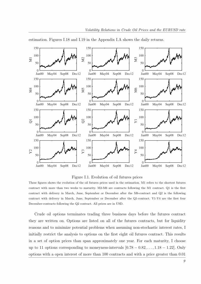
Crude oil options terminates trading three business days before the futures contract
they are written on. Options are listed on all of the futures contracts, but for liquidity
reasons and to minimize potential problems when assuming non-stochastic interest rates, I
initially restrict the analysis to options on the first eight oil futures contract. This results
in a set of option prices than span approximately one year. For each maturity, I choose
up to 11 options corresponding to moneyness-intervals [0.78 − 0.82, . . . , 1.18 − 1.22]. Only
options with a open interest of more than 100 contracts and with a price greater than 0.01
9

I.2. Overview of data
Jan00 May04 Sep08 Dec12
Q1
0.8
1
1.2
1.4
1.6
Jan00 May04 Sep08 Dec12
Q2
0.8
1
1.2
1.4
1.6
Jan00 May04 Sep08 Dec12
Q3
0.8
1
1.2
1.4
1.6
Jan00 May04 Sep08 Dec12
Q4
0.8
1
1.2
1.4
1.6
Jan00 May04 Sep08 Dec12
Q5
0.8
1
1.2
1.4
1.6
Jan00 May04 Sep08 Dec12
Q6
0.8
1
1.2
1.4
1.6
Figure I.2. Evolution of EURUSD futures pricesThese figures shows the evolution of the EURUSD futures prices used in the estimation. Q1 refers to the shortest
futures contract maturing more than a week later. Q2-Q6 are the contracts delivering 3-15 months after Q1 futures
contract. All expiry dates are in the March-cycle. Availability of prices in the long end of the futures is limited for
the first couple of years. By definition, the EURUSD rate is the price of EUR measured in USD.
10
Volatility Relations in Crude Oil Prices and the EURUSD rate
are included. For moneyness-intervals less than one, only put options are chosen and for
moneyness-intervals greater than one, only call options are included in the dataset. For the
moneyness-interval including 1, the most liquid option is chosen. Within each moneyness-
interval, the option closest to the mean of the interval is chosen based the aforementioned
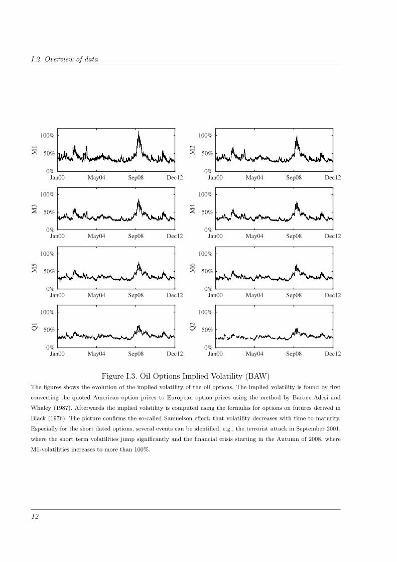
criteria. The number of days with observations, implied volatilities, average prices and open
interest are summarized in the tables in Appendix I.A and the ATM implied volatilities
are plotted in Figure I.3. The Samuelson effect – that futures with short time to expiry are
more volatile compared to options with long time to expiry – is clearly seen by comparing
across maturities. Further, volatility is evidently stochastic.
EURUSD options are traded on the first four quarterly futures contracts. The options
with expiry in the same month as the underlying are denoted Q1-Q4. In addition, two nearby
monthly options on the nearby futures are also traded: For instance, in early January, the
closest futures contract is the March contract. Besides options expiring in March, the first
monthly option, M1, expires in January with the March futures as underlying. The second
monthly option, M2, is a February option on the March futures contract. When the January
option expires, the February option on the March futures becomes the M1 contract and an
April option on the June futures become the M2 contract. See Figure I.4 for an illustration
of existence and labelling of EURUSD options. The options expire on the Friday 12 days
before the third Wednesday of the option’s contract month. Like with the oil options, the
sorting results in a set of option prices than span approximately one year. The final set of
EURUSD options data is chosen using the same guidelines as with the oil options data. The
resulting dataset is summarized in tables I.10-I.16 in Appendix I.A, and the ATM implied
volatility is plotted in Figure I.5.
Both the oil option prices and the EURUSD options are for American type options. The
impact of early exercise is small in the chosen sample, because only OTM and ATM options
were included. Nevertheless, the prices are still converted to European prices by converting
quoted American option prices to European option prices using the approach from Barone-
Adesi and Whaley (1987). All reported implied volatilities are for corresponding European
options.
By inspection of Tables I.9 and I.10, it become apparent that there is still a great deal
of asymmetry in the availability of option prices. The model-free analysis in Section I.3 is
based on ATM options resulting from the initial sorting. When turning to estimation using
multiple moneyness-intervals in Section I.5, the dataset is restricted further to ensure that
11
I.2. Overview of data
Jan00 May04 Sep08 Dec12
M1
0%
50%
100%
Jan00 May04 Sep08 Dec12
M2
0%
50%
100%
Jan00 May04 Sep08 Dec12
M3
0%
50%
100%
Jan00 May04 Sep08 Dec12
M4
0%
50%
100%
Jan00 May04 Sep08 Dec12
M5
0%
50%
100%
Jan00 May04 Sep08 Dec12
M6
0%
50%
100%
Jan00 May04 Sep08 Dec12
Q1
0%
50%
100%
Jan00 May04 Sep08 Dec12
Q2
0%
50%
100%
Figure I.3. Oil Options Implied Volatility (BAW)The figures shows the evolution of the implied volatility of the oil options. The implied volatility is found by first
converting the quoted American option prices to European option prices using the method by Barone-Adesi and
Whaley (1987). Afterwards the implied volatility is computed using the formulas for options on futures derived in
Black (1976). The picture confirms the so-called Samuelson effect; that volatility decreases with time to maturity.
Especially for the short dated options, several events can be identified, e.g., the terrorist attack in September 2001,
where the short term volatilities jump significantly and the financial crisis starting in the Autumn of 2008, where
M1-volatilities increases to more than 100%.
12

Volatility Relations in Crude Oil Prices and the EURUSD rate
Panel A: From start of December to start of JanuaryJan Feb Mar Jun Sep Dec
Future:
Option:
Underlying:
−
M1
Mar
−
M2
Mar
Q1
Q1
Mar
Q2
Q2
Jun
Q3
Q3
Sep
Q4
Q4
Dec
Panel B: From start of January to start of FebruaryFeb Mar Apr Jun Sep Dec
Future:
Option:
Underlying:
−
M1
Mar
Q1
Q1
Mar
-
M2
Jun
Q2
Q2
Jun
Q3
Q3
Sep
Q4
Q4
Dec
Panel C: From start of February to start of MarchMar Apr May Jun Sep Dec
Future:
Option:
Underlying:
Q1
Q1
Mar
−
M1
Jun
-
M2
Jun
Q2
Q2
Jun
Q3
Q3
Sep
Q4
Q4
Dec
Figure I.4. EURUSD contractsThis figure illustrates the existence and naming of options on EURUSD futures contracts. In Panel A, the M1- and
M2-options are written on the Q1-futures, but expiring 2 resp. 1 month before the underlying. The Q1–Q4-options
mature in the same months as their underlying. This happens from start of December to start of January, from start
of March to start of April, from start of June to start of July, and from start of September to start of October.
Panel B shows the situation where the M1-option is written on the Q1-futures and the M2-option is written on the
Q2-futures. This happens from start of January to start of February, from start of April to start of May, from start of
July to start of August, and from start of October to start of November. Finally, Panel C shows the situation where
the M1- and M2-options are written on the Q2-futures. This happens from start of February to start of March, from
start of May to start of June, from start of August to start of September, and from start of November to start of
December.
13

I.2. Overview of data
Jan00 May04 Sep08 Dec12
M1
0%
10%
20%
30%
40%
Jan00 May04 Sep08 Dec12
M2
0%
10%
20%
30%
40%
Jan00 May04 Sep08 Dec12
Q1
0%
10%
20%
30%
40%
Jan00 May04 Sep08 Dec12
Q2
0%
10%
20%
30%
40%
Jan00 May04 Sep08 Dec12
Q3
0%
10%
20%
30%
40%
Jan00 May04 Sep08 Dec12
Q4
0%
10%
20%
30%
40%
Figure I.5. EURUSD Options Implied Volatility (BAW)The figures shows the evolution of the implied volatility of the EURUSD options. The implied volatility is found
by first converting the quoted American option prices to European option prices using the method by Barone-Adesi
and Whaley (1987). Afterwards the implied volatility is computed using the formulas for options on futures derived
in Black (1976). Availability of liquid options in the long end is scarce. EURUSD volatility approximately double at
the beginning of the financial crisis.
14
Volatility Relations in Crude Oil Prices and the EURUSD rate
the volatility surfaces span a reasonable time frame and moneyness-intervals, while at the
same time not showing too much asymmetry in availability of data.
I.3 Model-free Analysis: Joint Volatility Factors
The investigation of a joint factor in the volatility of crude oil and the volatility of EURUSD
starts with a model-free analysis: I construct oil ATM straddle returns by calculating daily
prices of ATM straddles, i.e., a put and a call option with strike equal to the value of
the underlying futures, with 1-6 months to maturity. The first oil five straddles are on
the nearest futures contract expiring approximately one month after the options and the
6M-straddle is on the futures contract in the March cycle that expires 7-9 months out.
Similarly, straddle returns for EURUSD are calculated for contracts with 1-5 months to
maturity with the nearest following futures contract as underlying. ATM straddles are by
construction approximately Delta-neutral, so they are almost unaffected by changes in the
underlying, but very sensitive to changes in volatility.
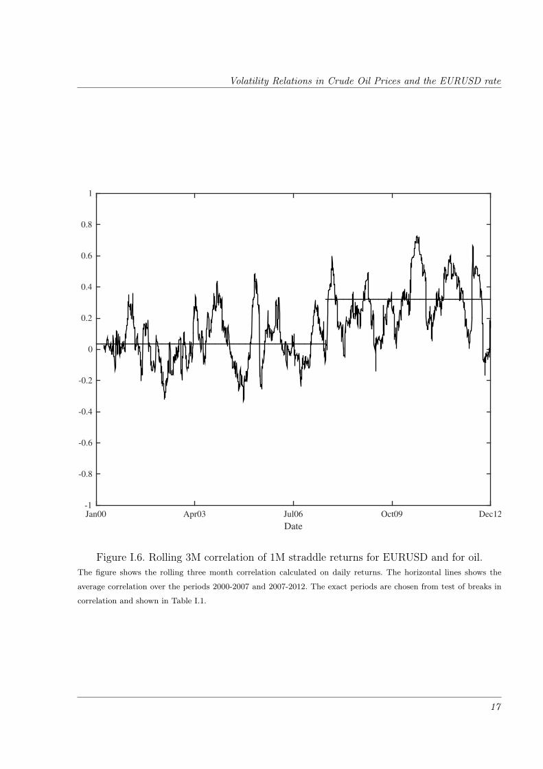
Figure I.6 shows the 3-month rolling correlation of the 1M-straddle returns. Over the
full period, the empirical full sample correlation is positive, 0.1718, but a visual inspection
of the rolling correlation indicates a development over time. To identify the possible change
points in the correlation, I employ the method proposed by Galeano and Wied (2014), which
is an extension of the test proposed in Wied et al. (2009). The method provide an algorithm
for detecting multiple breaks in correlation structure of random variables. For a sequence
of random variables (Xt,Yt), t ∈ [1, . . . ,T ] with correlation between Xt and Yt denoted by
ρt, the hypothesis of all correlations being equal is tested using the test statistic
QT (X,Y ) = D max2≤j≤T
j√T|ρj − ρT |,
where ρj is the empirical correlation up to time j and D is a normalising constant. The
asymptotic distribution of the test statistic is the supremum of the absolute value of a
standard Brownian bridge. For a critical level of 5%, the test statistic is compared to a value
of 1.358. The algorithm described in Galeano and Wied (2014) is an iterative procedure,
where the test statistic is first obtained for the full sample size. If the test statistic is
significant, the break point obtained from the test size is determined a break in correlation
and the resulting two samples are tested separately. This procedure is continued until no
15
I.3. Model-free Analysis: Joint Volatility Factors
further breaks are obtained6. Finally, adjoining sub-samples are tested pairwise to assess if
the estimated break point is optimal. If not, the original break point is replaced by the new
optimal break point.
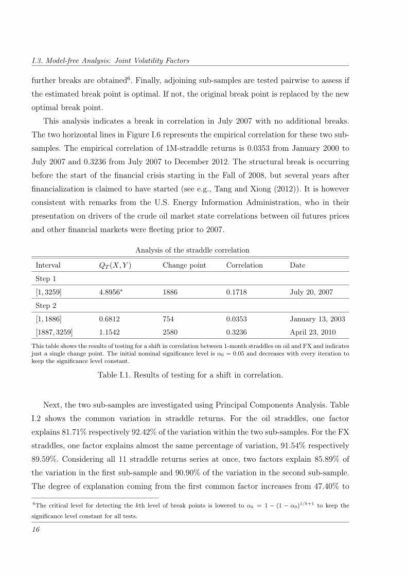
This analysis indicates a break in correlation in July 2007 with no additional breaks.
The two horizontal lines in Figure I.6 represents the empirical correlation for these two sub-
samples. The empirical correlation of 1M-straddle returns is 0.0353 from January 2000 to
July 2007 and 0.3236 from July 2007 to December 2012. The structural break is occurring
before the start of the financial crisis starting in the Fall of 2008, but several years after
financialization is claimed to have started (see e.g., Tang and Xiong (2012)). It is however
consistent with remarks from the U.S. Energy Information Administration, who in their
presentation on drivers of the crude oil market state correlations between oil futures prices
and other financial markets were fleeting prior to 2007.
Analysis of the straddle correlation
Interval QT (X,Y ) Change point Correlation Date
Step 1
[1, 3259] 4.8956∗ 1886 0.1718 July 20, 2007
Step 2
[1, 1886] 0.6812 754 0.0353 January 13, 2003
[1887, 3259] 1.1542 2580 0.3236 April 23, 2010
This table shows the results of testing for a shift in correlation between 1-month straddles on oil and FX and indicatesjust a single change point. The initial nominal significance level is α0 = 0.05 and decreases with every iteration tokeep the significance level constant.
Table I.1. Results of testing for a shift in correlation.
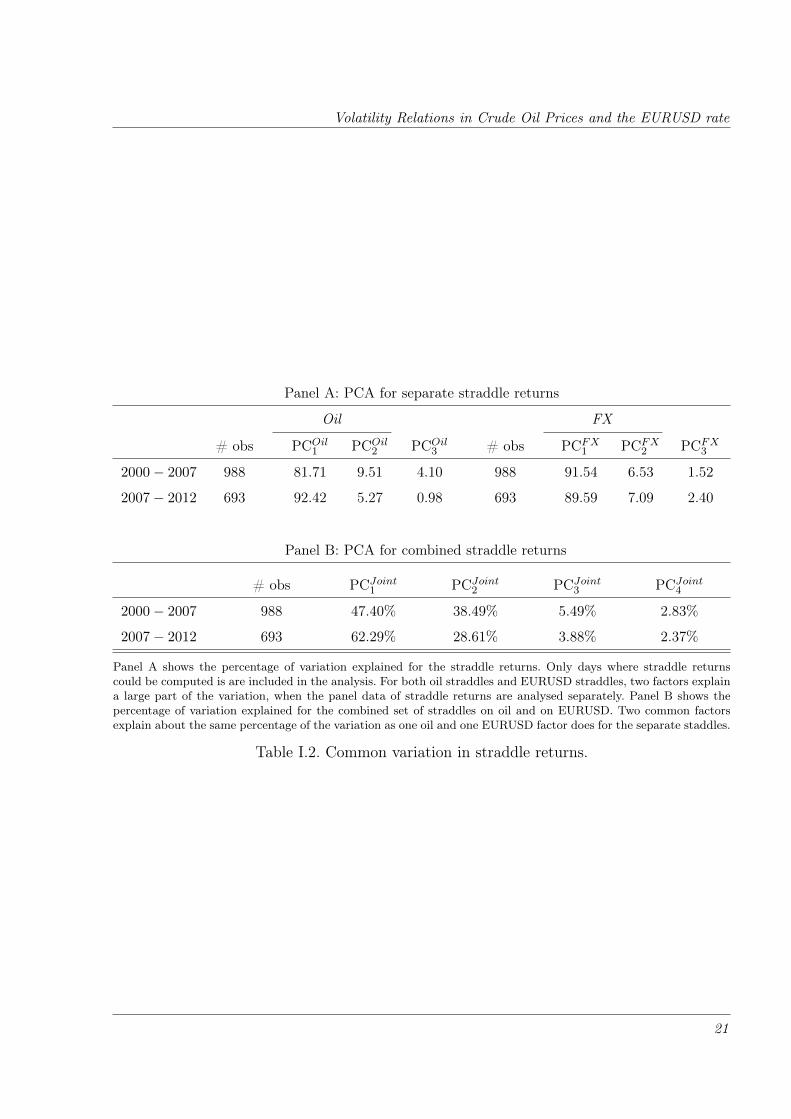
Next, the two sub-samples are investigated using Principal Components Analysis. Table
I.2 shows the common variation in straddle returns. For the oil straddles, one factor
explains 81.71% respectively 92.42% of the variation within the two sub-samples. For the FX
straddles, one factor explains almost the same percentage of variation, 91.54% respectively
89.59%. Considering all 11 straddle returns series at once, two factors explain 85.89% of
the variation in the first sub-sample and 90.90% of the variation in the second sub-sample.
The degree of explanation coming from the first common factor increases from 47.40% to
6The critical level for detecting the kth level of break points is lowered to αk = 1 − (1 − α0)1/k+1 to keep the
significance level constant for all tests.
16
Volatility Relations in Crude Oil Prices and the EURUSD rate
Date
Jan00 Apr03 Jul06 Oct09 Dec12-1
-0.8
-0.6
-0.4
-0.2
0
0.2
0.4
0.6
0.8
1
Figure I.6. Rolling 3M correlation of 1M straddle returns for EURUSD and for oil.The figure shows the rolling three month correlation calculated on daily returns. The horizontal lines shows the
average correlation over the periods 2000-2007 and 2007-2012. The exact periods are chosen from test of breaks in
correlation and shown in Table I.1.
17
I.3. Model-free Analysis: Joint Volatility Factors
62.29%.
The above numbers do not guarantee that there is co-variation between straddle returns.
To ensure that the two first factors is the combined PCA is not merely one factor for
crude oil and one factor for EURUSD, the eigenvectors for the first three joint principal
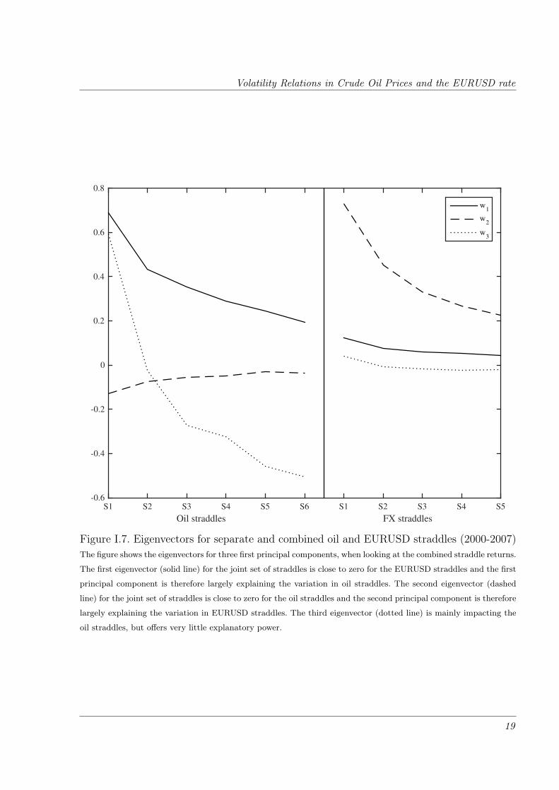
components are presented in Figures I.7 and I.8. For the first sub-sample (Figure I.7),
the first joint principal component mainly explains the variations in the oil straddles, as
the eigenvector values related to the EURUSD straddles is close to zero. The second joint
principal component mainly explains the variations in the EURUSD straddle returns. There
is little indication of a common factor driving the two sets of straddle returns and thereby
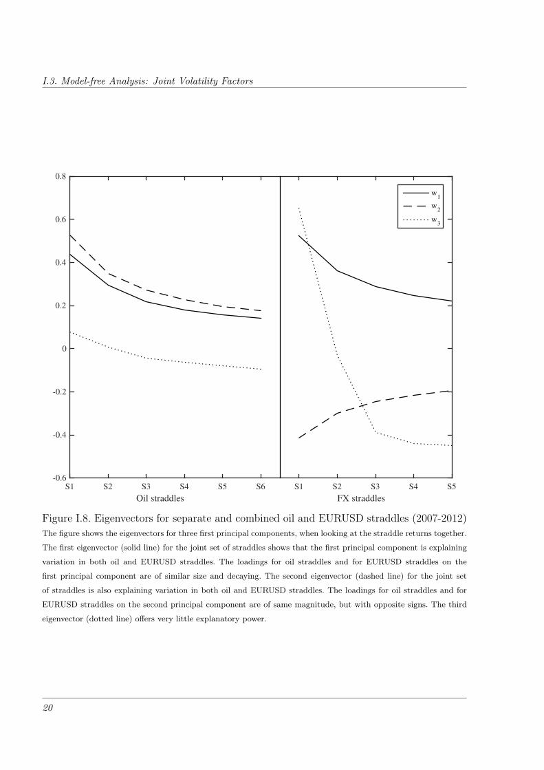
the volatilities of crude oil and EURUSD. For the second sub-sample (Figure I.8) staring
in July 2007, the picture is different: The first joint principal component, that explains
62.29% of the total variation in the combined straddles, affect both the oil straddles and the
EURUSD straddles. The second principal component also explains variation in both oil and
EURUSD straddles, but with opposite signs for oil straddles and EURUSD straddles. The
eigenvector is decaying in maturity of the straddles, which is in line with the Samuelson-
effect; volatilities (or equivalent straddle returns) are higher for shorter maturities compared
to longer maturities.
In conclusion, the model free analysis in this section empirically considers the rolling
correlation of short crude oil straddles and short EURUSD straddles and confirms that
volatilities (more precisely in the form of straddle returns) exhibit a much higher correlation
during the later part of the period analysed compared to the beginning.
Secondly, a Principal Components Analysis shows that around 85-90% of the variation
across combined straddle returns can be explained using two factors. For the first sub-sample
one factor is attributed to explaining the oil straddles and a second factor is attributed to
EURUSD straddles. For the second sub-sample, the two factors both contribute to explaining
the variation across the combined set of straddles.
In the next section, a model including a joint volatility factor is proposed. In total, there
will be three volatility factors; one joint volatility factor, one volatility factor for oil and one
volatility factor for EURUSD.
18
Volatility Relations in Crude Oil Prices and the EURUSD rate
Oil straddles FX straddles
S1 S2 S3 S4 S5 S6 S1 S2 S3 S4 S5-0.6
-0.4
-0.2
0
0.2
0.4
0.6
0.8
w1
w2
w3
Figure I.7. Eigenvectors for separate and combined oil and EURUSD straddles (2000-2007)The figure shows the eigenvectors for three first principal components, when looking at the combined straddle returns.
The first eigenvector (solid line) for the joint set of straddles is close to zero for the EURUSD straddles and the first
principal component is therefore largely explaining the variation in oil straddles. The second eigenvector (dashed
line) for the joint set of straddles is close to zero for the oil straddles and the second principal component is therefore
largely explaining the variation in EURUSD straddles. The third eigenvector (dotted line) is mainly impacting the
oil straddles, but offers very little explanatory power.
19
I.3. Model-free Analysis: Joint Volatility Factors
Oil straddles FX straddles
S1 S2 S3 S4 S5 S6 S1 S2 S3 S4 S5-0.6
-0.4
-0.2
0
0.2
0.4
0.6
0.8
w1
w2
w3
Figure I.8. Eigenvectors for separate and combined oil and EURUSD straddles (2007-2012)The figure shows the eigenvectors for three first principal components, when looking at the straddle returns together.
The first eigenvector (solid line) for the joint set of straddles shows that the first principal component is explaining
variation in both oil and EURUSD straddles. The loadings for oil straddles and for EURUSD straddles on the
first principal component are of similar size and decaying. The second eigenvector (dashed line) for the joint set
of straddles is also explaining variation in both oil and EURUSD straddles. The loadings for oil straddles and for
EURUSD straddles on the second principal component are of same magnitude, but with opposite signs. The third
eigenvector (dotted line) offers very little explanatory power.
20
Volatility Relations in Crude Oil Prices and the EURUSD rate
Panel A: PCA for separate straddle returns
Oil FX
# obs PCOil1 PCOil2 PCOil3 # obs PCFX1 PCFX2 PCFX3
2000− 2007 988 81.71 9.51 4.10 988 91.54 6.53 1.52
2007− 2012 693 92.42 5.27 0.98 693 89.59 7.09 2.40
Panel B: PCA for combined straddle returns
# obs PCJoint1 PCJoint2 PCJoint3 PCJoint4
2000− 2007 988 47.40% 38.49% 5.49% 2.83%
2007− 2012 693 62.29% 28.61% 3.88% 2.37%
Panel A shows the percentage of variation explained for the straddle returns. Only days where straddle returnscould be computed is are included in the analysis. For both oil straddles and EURUSD straddles, two factors explaina large part of the variation, when the panel data of straddle returns are analysed separately. Panel B shows thepercentage of variation explained for the combined set of straddles on oil and on EURUSD. Two common factorsexplain about the same percentage of the variation as one oil and one EURUSD factor does for the separate staddles.
Table I.2. Common variation in straddle returns.
21

I.4. A Linked Model for Derivatives on Oil and the EURUSD
I.4 A Linked Model for Derivatives on Oil and the EURUSD
In this paper, the model proposed by Trolle and Schwartz (2009) for oil derivatives is used
as a starting point7. It has proven to fit the market well as documented in the original paper
and tested for later years in Cortazar et al. (2016). To have a flexible and still tractable model
for the futures and option prices for both oil and FX, two models of the type developed in
Trolle and Schwartz (2009) is combined by allowing one of the two asset specific volatility
factors, υ, to be the same. As the focus is on the joint volatility factor, the number of factors
driving the futures prices are limited to decrease the number of parameters to be estimated.
This will favour the fit of options over the fit of the futures curve.
I.4.1 Model
Let Et denote the time-t spot price of oil with a spot cost-of-carry8 given by δEt . The
spot cost-of-carry is derived from the forward cost-of-carry yE, i.e., yEt (T ) is the time-t
instantaneous cost-of-carry between t and T and δEt = yEt (t). Under the (domestic) risk
neutral measure, the oil price (measured in the domestic currency) isdEtEt
= δEt dt+ σE1
√υEt dW
Et + σE2
√υJt dW
Jt (I.1)
dyEt (T ) = µE(t,T ) + αEe−γE(T−t)
√υEt dB
Et (I.2)
Correspondingly, Xt denotes the time-t EURUSD exchange rate with an spot interest rate
differential given by δXt . The interest rate differential is derived from the forward interest
rate differential yX , i.e., yXt (T ) is the time-t forward rate differential and δXt = yXt (t). Under
the risk neutral measure, the EURUSD rate (i.e., the price of EUR measured in the USD)
isdXt
Xt
= δXt dt+ σX1
√υXt dW
Xt + σX2
√υJt dW
Jt (I.3)
dyXt (T ) = µX(t,T ) + αXe−γX(T−t)
√υXt dB
Xt (I.4)
The three volatility factors evolve according to
dυEt =(ηE − κEυEt
)dt+ συE
√υEt dZ
Et (I.5)
7Another approach would have been to extend the approach taken in Pilz and Schlögl (2012), who they apply
a multi-LIBOR model applied to one interest rate and the oil price. An extension of the would be to include an
additional interest rate and thereby modelling the FX rate through the two interest rates.8The cost-of-carry is defined as the interest rate net of the convenience yield
22
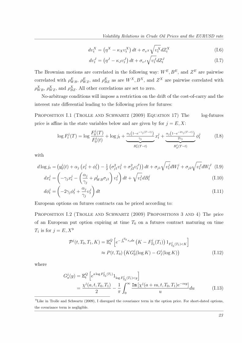
Volatility Relations in Crude Oil Prices and the EURUSD rate
dυXt =(ηX − κXυXt
)dt+ συX
√υXt dZ
Xt (I.6)
dυJt =(ηJ − κJυJt
)dt+ συJ
√υJt dZ
Jt (I.7)
The Brownian motions are correlated in the following way: WE,BE, and ZE are pairwise
correlated with ρEWB, ρEWZ , and ρEBZ as are WX ,BX , and ZX are pairwise correlated with
ρXWB, ρXWZ , and ρXBZ . All other correlations are set to zero.
No-arbitrage conditions will impose a restriction on the drift of the cost-of-carry and the
interest rate differential leading to the following prices for futures:
Proposition I.1 (Trolle and Schwartz (2009) Equation 17) The log-futures
price is affine in the state variables below and are given by for j = E,X:
logF jt (T ) = log
F j0 (T )
F j0 (t)
+ log jt +αj(1−e−γj(T−t))
γj︸ ︷︷ ︸Bjx(T−t)
xjt +αj(1−e−2γj(T−t))
2γj︸ ︷︷ ︸Bjφ(T−t)
φjt (I.8)
with
d log jt =(yj0(t) + αj
(xjt + φjt
)− 1
2
(σ2j1υ
jt + σ2
j2υJt
))dt+ σj1
√υjtdW
jt + σj2
√υJt dW
Jt (I.9)
dxjt =
(−γjxjt −
(αjγj
+ ρjWBσj1
)υjt
)dt+
√υjtdB
jt (I.10)
dφjt =
(−2γjφ
jt +
αjγjυjt
)dt (I.11)
European options on futures contracts can be priced according to:
Proposition I.2 (Trolle and Schwartz (2009) Propositions 3 and 4) The price
of an European put option expiring at time T0 on a futures contract maturing on time
T1 is for j = E,X9
Pj(t,T0,T1,K) = EQt[e−
∫ T0t rsds
(K − F j
T0(T1)
)1F jT0
(T1)<K
]≈ P (t,T0)
(KGj
0(logK)−Gj1(logK)
)(I.12)
where
Gja(y) = EQt
[ea logF jT0
(T1)1logF jT0(T1)<y
]=χj(a, t,T0,T1)
2− 1
π
∫ ∞0
Im [χj(a+ ıu, t,T0,T1)e−ıuy]
udu (I.13)
9Like in Trolle and Schwartz (2009), I disregard the covariance term in the option price. For short-dated options,
the covariance term is negligible.
23
I.4. A Linked Model for Derivatives on Oil and the EURUSD
and the transform χ is given as
χj(u, t,T0,T1) = EQt[eu logF jT0
(T1)]
,
with an exponentially affine solution given by
χj(u, t,T0,T1) = eMj(T0−t)+N1j(T0−t)υjt+N2j(T0−t)υJt +u logF jt (T1). (I.14)
where Mj and Nj are solutions to the following ODEs:
M ′j(τ) =N1j(τ)ηj +N2j(τ)ηJ
N ′j1(τ) =12(u2 − u)
[σ2j1 +Bj
x(T1 − T0 + τ)2 + 2ρjWBσj1Bjx(T1 − T0 + τ)
]+Nj1(τ)
[−κj + uσυj
(ρjWZσj1 + ρjBZB
jx(T1 − T0 + τ)
)]+ 1
2Nj1(τ)2σ2
υj
N ′j2(τ) =12(u2 − u)σ2
j2 −Nj2(τ)κJ + 12Nj2(τ)2σ2
υJ
subject to the boundary conditions Mj(0) = Nj1(τ) = Nj2(τ) = 0. In practice the integral
is evaluated in a set of cleverly chosen points, e.g., using the Gauss-Legendre quadrature.
For the joint model, this results in 34 parameters. In case σE2 = σX2 = 0, each asset
is modelled using the SV1-specification in Trolle and Schwartz (2009) and 14 parameters
for each model is then needed. The six extra parameters are the loadings of the spot oil
price and spot EURUSD rate on the joint volatility factor, the speed (and thereby mean-
reversion level) and the volatility of the joint volatility process as well as the market price
of risk belonging to the two extra Brownian motions10.
Using this specification, only the spot price is affected by the joint volatility, whereas
the shape of the futures curve is not. For simplicity the three stochastic volatility processes
are not connected via their drift. Another possible specification would be to let the separate
oil volatility and the separate EURUSD volatility process mean reverts around the joint
volatility process. In this situation, the joint volatility process would not need to enter into
the spot price specification, but could be obtained from the joint volatility process affecting
the future volatility and thereby the option prices.
10It might seem unnecessary restrictive to include the same Brownian motion in the two spot dynamics, but the
estimation showed very little difference in the likelihood function when the same Brownian motion was used compared
to two different and correlated Brownian motions.
24
Volatility Relations in Crude Oil Prices and the EURUSD rate
I.4.2 Estimation Approach
The model is estimated using quasi maximum-likelihood applying the extended Kalman
filter after formulating the model in state-space form11. The observed log futures prices and
the option prices are linked to the state vector through the measurement equation
yt =h(θt) + εt, εt ∼ N (0, Ω) (I.15)
where yt is a vector of observed prices, h is the pricing functions given by (I.8) and (I.12) and
εt are assumed i.i.d. Gaussian measurement errors with covariance matrix Ω. It is assumed
that measurement errors are uncorrelated, implying that Ω is a diagonal matrix and that
each of the four contract types has the same variance of the measurement error. The states
θt =(logEt,x
Et ,φEt , υEt , logXt,x
Xt ,φXt , υXt , υJt
)′has the following transition equation
θt+1 = Tθt + c+ εt+1 (I.16)
with Et(εt+1) = 0 and Covt(εt+1) = Q0 + QEυEt + QXυXt + QJυJt . The state vector needs
to be specified under the physical probability measure, which is obtained by specifying the
market prices of risk to link the Brownian motions under P (indicated by a ) and Q. The
completely affine specification is commonly used in this class of models:
dW jt =dW j
t − λjW
√υjtdt (I.17)
dW Jt =dW J
t − λJW√υJt dt (I.18)
dBjt =dBj
t − λjB
√υjtdt (I.19)
dZjt =dZj
t − λjZ
√υjtdt (I.20)
The vector c and the matrices and T , Q0, QE, QX and QJ are available in closed form and
derived using (I.9)-(I.11) and (I.5)-(I.7) together with the market price of risk specification.
The details can be found in Appendix I.B.
At time t, mE oil futures prices and nE oil option prices are observed along with the spot
FX rate, mX FX futures prices and nX FX option prices. To convert option pricing errors
11Details related to the application of Kalman filters can be found in classic references such as Harvey (1989).
25
I.5. Results
to implied volatility errors, the option prices are scaled by their vegas, so the observations
zt are given by
zt =(
logFEt (T1), . . . , logFE
t (TmE),OE,1t /VE,1
t , . . . ,OE,nE
t /VE,nE
t ,
logXt, logFXt (T1), . . . , logFX
t (TmX ),OX,1t /VX,1
t , . . . ,OX,nX
t /VX,nX
t
)′Finally as it is standard in this type of estimation, see e.g., Trolle and Schwartz (2009) and
Chiarella et al. (2013), a time-homogeneous version of (I.8) is considered by assuming that
the initial cost-of-carry, yE0 (T ), and interest rate differential, yX0 (T ), are flat: yE0 (T ) = ξE
and yE0 (T ) = ξX for all maturities T . To ensure identification, η is set to 1 for all volatility
processes .
I.5 Results
The joint likelihood function will favour the fit of oil options more, if the dataset is kept as it
is after the initial sorting as there are more oil option observations. To ensure a reasonable
surface without too much asymmetry in the number of contracts, the dataset is further
limited: The estimation is done on the middle five moneyness intervals, i.e., ranging from 0.9
to 1.1. For oil, options on M1-M6 is included and for EURUSD, options on M1-M2 and Q1-
Q2 is used. This gives a maturity span of just over six months. Further, the EURUSD options
with less than 10 trading days to maturity is taken out, as the fitting procedure by scaling
option prices with Vega is sensitive to short maturities. For the EURUSD options, there is
very limited availability of options for the two outermost moneyness intervals during the first
sub-sample. The discount rate in the option pricing formula is obtained by interpolation of
the 1-month, 3-month, 6-month and 1-year LIBOR-rates and the 2-year swap rate. Interest
rate data is downloaded from the Federal Reserve Bank of St. Louis.
I.5.1 Estimation results
Before the full model is estimated presented in Section I.4, the model is estimated using only
one volatility factor for the oil futures and options sample and for the EURUSD futures and
options sample. The figures in Figure I.9 show the filtered time series of υEt and υXt , when
the models are estimated separately for each of the two sub-samples. During the first sub-
sample, the processes seem unrelated. The empirical correlation of changes in the volatility
processes is 0.0444. During the second sub-sample, the processes exhibit similarities and
26
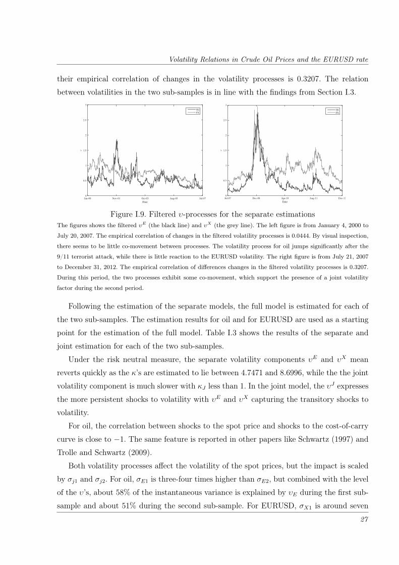
Volatility Relations in Crude Oil Prices and the EURUSD rate
their empirical correlation of changes in the volatility processes is 0.3207. The relation
between volatilities in the two sub-samples is in line with the findings from Section I.3.
Date
Jan-00 Nov-01 Oct-03 Aug-05 Jul-07
υ
0
0.5
1
1.5
2
2.5
3
Oil
FX
Date
Jul-07 Dec-08 Apr-10 Aug-11 Dec-12
υ
0
0.5
1
1.5
2
2.5
3
Oil
FX
Figure I.9. Filtered υ-processes for the separate estimationsThe figures shows the filtered υE (the black line) and υX (the grey line). The left figure is from January 4, 2000 to
July 20, 2007. The empirical correlation of changes in the filtered volatility processes is 0.0444. By visual inspection,
there seems to be little co-movement between processes. The volatility process for oil jumps significantly after the
9/11 terrorist attack, while there is little reaction to the EURUSD volatility. The right figure is from July 21, 2007
to December 31, 2012. The empirical correlation of differences changes in the filtered volatility processes is 0.3207.
During this period, the two processes exhibit some co-movement, which support the presence of a joint volatility
factor during the second period.
Following the estimation of the separate models, the full model is estimated for each of
the two sub-samples. The estimation results for oil and for EURUSD are used as a starting
point for the estimation of the full model. Table I.3 shows the results of the separate and
joint estimation for each of the two sub-samples.
Under the risk neutral measure, the separate volatility components υE and υX mean
reverts quickly as the κ’s are estimated to lie between 4.7471 and 8.6996, while the the joint
volatility component is much slower with κJ less than 1. In the joint model, the υJ expresses
the more persistent shocks to volatility with υE and υX capturing the transitory shocks to
volatility.
For oil, the correlation between shocks to the spot price and shocks to the cost-of-carry
curve is close to −1. The same feature is reported in other papers like Schwartz (1997) and
Trolle and Schwartz (2009).
Both volatility processes affect the volatility of the spot prices, but the impact is scaled
by σj1 and σj2. For oil, σE1 is three-four times higher than σE2, but combined with the level
of the υ’s, about 58% of the instantaneous variance is explained by υE during the first sub-
sample and about 51% during the second sub-sample. For EURUSD, σX1 is around seven
27

I.5. Results
times higher than σX2 during the first sub-sample and υX explains 96% of the variance.
During the second sub-sample, the ratio of σX ’s decreases to four and υX now explains only
86% of the variance.
The separate models are per construction not connected. Estimating the two models
jointly will give the value of the log-likelihood function as the sum of the two separate log-
likelihood functions. This model would be nested in the full model and it would therefore
be possible to test the parameter restriction in the separate models using likelihood ratio
tests. Given the large number of observations, the separate models would be rejected at
high levels of statistical significance. Instead the pricing performance is compared both at
an aggregated level, where time series of root mean squared errors are time series of errors
are investigated, and later in Section I.5.2 for each combination of moneyness interval and
maturity.
Based on the filtered values of the latent processes, fitted futures prices and log-normal
implied volatilities are computed and compared to actual values. The figures showing the
time series of RMSEs for oil futures in Figure I.10 and for EURUSD futures in Figure I.11
are very similar. This is not surprising, as the additional volatility factor only affects the
futures prices through the spot price.
Adding the extra volatility factor instead benefits the fit of the option prices. Table I.4
presents the results on an aggregated level: The average12 RMSE of the actual and fitted
log-normal implied volatilities decrease from 1.558% to 1.072% for the oil options in the
first period. For the same period, average RMSE of the actual and fitted log-normal implied
volatilities for EURUSD remain almost unchanged in the two specifications. For the second
sub-sample, there is both a decrease in oil option RMSE and EURUSD option RMSE. The
oil option RMSE decrease from 2.068% to 1.572% which is about 25 percent in the relative
terms. The EURUSD option RMSE from 0.809% to 0.766% which is about 5 percent in
relative terms. Together with the summary of RMSEs, Table I.4 also presents the results of
the test from by Diebold and Mariano (1995), where two time siries of RMSEs are compared:
The pairs of time series of RMSEs obtained by the separate and the full models are compared
by computing the mean of the differences between the separate and joint model and the
associated t-statistics. If the mean is significantly positive, the joint model provides a better
fit. The tests show that for the first sub-sample, oil options are significantly better fitted by
12The daily RMSE are the root of the mean of the squared errors from all options fitted on that day. The average
RMSE is the average of the daily RMSEs.
28
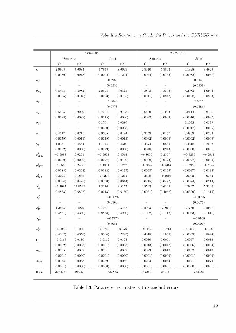
Volatility Relations in Crude Oil Prices and the EURUSD rate
2000-2007 2007-2012
Separate Joint Separate Joint
Oil FX Oil FX Oil FX Oil FX
κj 2.0908 7.6684 4.7948 8.6699 2.5370 5.5802 6.1828 8.4629
(0.0380) (0.0978) (0.0002) (0.1204) (0.0064) (0.0762) (0.0082) (0.0937)
κJ – – 0.8985 – – 0.6140
– – (0.0238) – – (0.0139)
συj 0.8458 0.3982 2.0994 0.6345 0.8858 0.8866 3.2983 1.0904
(0.0155) (0.0118) (0.0023) (0.0166) (0.0011) (0.0242) (0.0128) (0.0293)
συJ – – 2.3840 – – 2.6616
– – (0.0778) – – (0.0384)
σj1 0.5385 0.2059 0.7064 0.2103 0.6439 0.1963 0.8114 0.2401
(0.0028) (0.0029) (0.0015) (0.0036) (0.0022) (0.0034) (0.0016) (0.0027)
σj2 – – 0.1791 0.0289 – – 0.1052 0.0259
– – (0.0030) (0.0008) – – (0.0017) (0.0005)
αj 0.4317 0.0215 0.9305 0.0194 0.3449 0.0157 0.4709 0.0204
(0.0079) (0.0011) (0.0019) (0.0013) (0.0032) (0.0008) (0.0062) (0.0009)
γj 1.0131 0.4534 1.1174 0.4310 0.4374 0.0836 0.4318 0.2592
(0.0052) (0.0080) (0.0029) (0.0080) (0.0048) (0.0243) (0.0000) (0.0031)
ρjWB −0.9098 0.6201 −0.9651 0.4544 −0.8050 0.2337 −0.9283 −0.2911
(0.0050) (0.0266) (0.0027) (0.0450) (0.0082) (0.0423) (0.0027) (0.0050)
ρjWZ −0.3503 0.2466 −0.1881 0.1757 −0.5842 −0.4437 −0.2958 −0.5142
(0.0085) (0.0203) (0.0032) (0.0157) (0.0063) (0.0124) (0.0037) (0.0132)
ρjBZ 0.3095 0.1888 −0.0278 0.1271 0.3598 −0.1004 0.0032 0.0382
(0.0184) (0.0425) (0.0130) (0.0644) (0.0215) (0.0422) (0.0024) (0.0214)
λjZ −0.1987 14.8593 1.2216 3.5157 2.8523 6.6109 4.3867 5.2140
(0.4863) (0.6807) (0.0013) (0.6160) (0.0061) (0.4058) (0.0399) (0.1416)
λJZ – – −0.0028 – – −0.0396
– – (0.2563) – – (0.0075)
λjW 1.2568 0.4929 0.7767 0.3167 0.5043 −2.8914 0.7739 0.5947
(0.4861) (0.4350) (0.8858) (0.4950) (0.1032) (0.1718) (0.0083) (0.1611)
λJW – – −0.7173 – – −0.8766
– – (0.3051) – – (0.0006)
λjB −0.5958 0.1020 −2.5758 −3.9569 −2.8832 −1.6761 −4.6689 −6.5189
(0.4862) (0.4358) (0.8184) (0.7293) (0.4075) (0.1068) (0.0069) (0.5644)
ξj −0.0167 0.0119 −0.0112 0.0123 0.0080 0.0091 0.0057 0.0012
(0.0002) (0.0003) (0.0001) (0.0003) (0.0013) (0.0042) (0.0006) (0.0004)
σfut 0.0135 0.0009 0.0131 0.0009 0.0093 0.0010 0.0102 0.0010
(0.0001) (0.0000) (0.0001) (0.0000) (0.0001) (0.0000) (0.0001) (0.0000)
σopt 0.0164 0.0053 0.0089 0.0052 0.0204 0.0084 0.0121 0.0079
(0.0001) (0.0000) (0.0000) (0.0000) (0.0001) (0.0001) (0.0000) (0.0001)
logL 206275 96927 333883 147250 86418 252035
Table I.3. Parameter estimates with standard errors
29
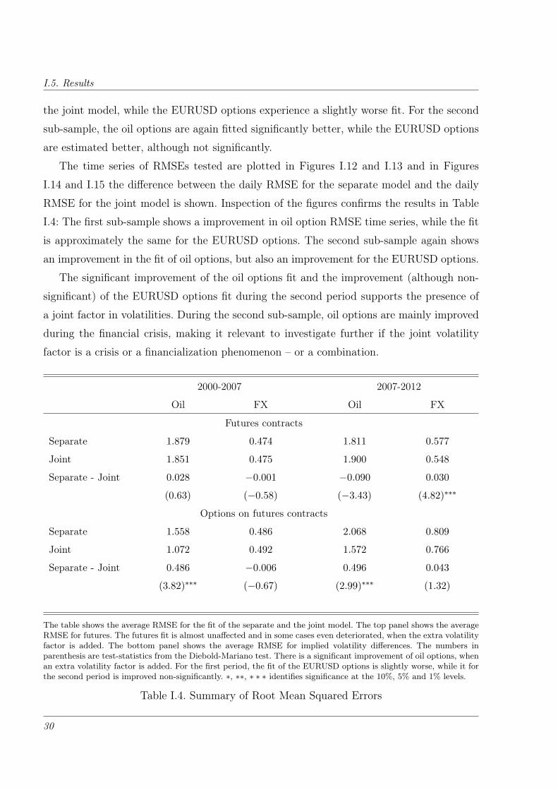
I.5. Results
the joint model, while the EURUSD options experience a slightly worse fit. For the second
sub-sample, the oil options are again fitted significantly better, while the EURUSD options
are estimated better, although not significantly.
The time series of RMSEs tested are plotted in Figures I.12 and I.13 and in Figures
I.14 and I.15 the difference between the daily RMSE for the separate model and the daily
RMSE for the joint model is shown. Inspection of the figures confirms the results in Table
I.4: The first sub-sample shows a improvement in oil option RMSE time series, while the fit
is approximately the same for the EURUSD options. The second sub-sample again shows
an improvement in the fit of oil options, but also an improvement for the EURUSD options.
The significant improvement of the oil options fit and the improvement (although non-
significant) of the EURUSD options fit during the second period supports the presence of
a joint factor in volatilities. During the second sub-sample, oil options are mainly improved
during the financial crisis, making it relevant to investigate further if the joint volatility
factor is a crisis or a financialization phenomenon – or a combination.
2000-2007 2007-2012
Oil FX Oil FX
Futures contracts
Separate 1.879 0.474 1.811 0.577
Joint 1.851 0.475 1.900 0.548
Separate - Joint 0.028 −0.001 −0.090 0.030
(0.63) (−0.58) (−3.43) (4.82)∗∗∗
Options on futures contracts
Separate 1.558 0.486 2.068 0.809
Joint 1.072 0.492 1.572 0.766
Separate - Joint 0.486 −0.006 0.496 0.043
(3.82)∗∗∗ (−0.67) (2.99)∗∗∗ (1.32)
The table shows the average RMSE for the fit of the separate and the joint model. The top panel shows the averageRMSE for futures. The futures fit is almost unaffected and in some cases even deteriorated, when the extra volatilityfactor is added. The bottom panel shows the average RMSE for implied volatility differences. The numbers inparenthesis are test-statistics from the Diebold-Mariano test. There is a significant improvement of oil options, whenan extra volatility factor is added. For the first period, the fit of the EURUSD options is slightly worse, while it forthe second period is improved non-significantly. ∗, ∗∗, ∗ ∗ ∗ identifies significance at the 10%, 5% and 1% levels.
Table I.4. Summary of Root Mean Squared Errors
30
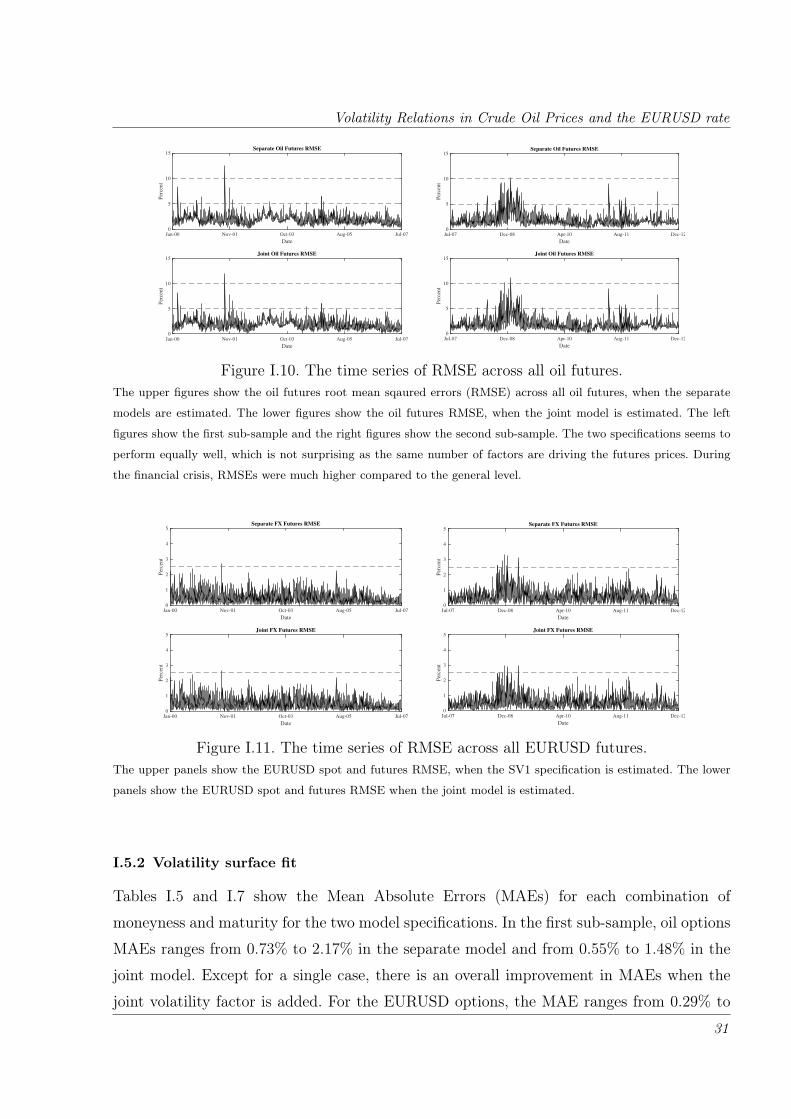
Volatility Relations in Crude Oil Prices and the EURUSD rate
Date
Jan-00 Nov-01 Oct-03 Aug-05 Jul-07
Per
cent
0
5
10
15Separate Oil Futures RMSE
Date
Jan-00 Nov-01 Oct-03 Aug-05 Jul-07
Per
cent
0
5
10
15Joint Oil Futures RMSE
Date
Jul-07 Dec-08 Apr-10 Aug-11 Dec-12
Per
cent
0
5
10
15Separate Oil Futures RMSE
Date
Jul-07 Dec-08 Apr-10 Aug-11 Dec-12
Per
cent
0
5
10
15Joint Oil Futures RMSE
Figure I.10. The time series of RMSE across all oil futures.The upper figures show the oil futures root mean sqaured errors (RMSE) across all oil futures, when the separate
models are estimated. The lower figures show the oil futures RMSE, when the joint model is estimated. The left
figures show the first sub-sample and the right figures show the second sub-sample. The two specifications seems to
perform equally well, which is not surprising as the same number of factors are driving the futures prices. During
the financial crisis, RMSEs were much higher compared to the general level.
Date
Jan-00 Nov-01 Oct-03 Aug-05 Jul-07
Per
cen
t
0
1
2
3
4
5Separate FX Futures RMSE
Date
Jan-00 Nov-01 Oct-03 Aug-05 Jul-07
Per
cen
t
0
1
2
3
4
5Joint FX Futures RMSE
Date
Jul-07 Dec-08 Apr-10 Aug-11 Dec-12
Per
cent
0
1
2
3
4
5Separate FX Futures RMSE
Date
Jul-07 Dec-08 Apr-10 Aug-11 Dec-12
Per
cent
0
1
2
3
4
5Joint FX Futures RMSE
Figure I.11. The time series of RMSE across all EURUSD futures.The upper panels show the EURUSD spot and futures RMSE, when the SV1 specification is estimated. The lower
panels show the EURUSD spot and futures RMSE when the joint model is estimated.
I.5.2 Volatility surface fit
Tables I.5 and I.7 show the Mean Absolute Errors (MAEs) for each combination of
moneyness and maturity for the two model specifications. In the first sub-sample, oil options
MAEs ranges from 0.73% to 2.17% in the separate model and from 0.55% to 1.48% in the
joint model. Except for a single case, there is an overall improvement in MAEs when the
joint volatility factor is added. For the EURUSD options, the MAE ranges from 0.29% to
31
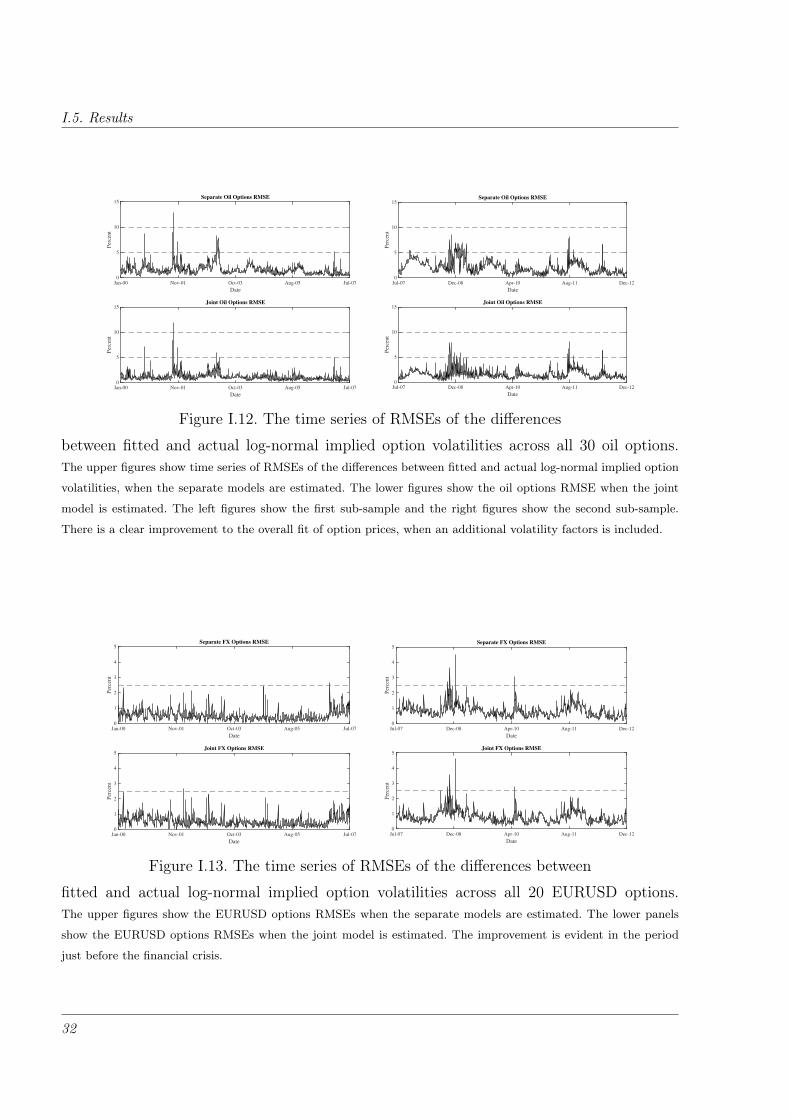
I.5. Results
Date
Jan-00 Nov-01 Oct-03 Aug-05 Jul-07
Per
cent
0
5
10
15Separate Oil Options RMSE
Date
Jan-00 Nov-01 Oct-03 Aug-05 Jul-07
Per
cent
0
5
10
15Joint Oil Options RMSE
Date
Jul-07 Dec-08 Apr-10 Aug-11 Dec-12
Per
cent
0
5
10
15Separate Oil Options RMSE
Date
Jul-07 Dec-08 Apr-10 Aug-11 Dec-12P
erce
nt
0
5
10
15Joint Oil Options RMSE
Figure I.12. The time series of RMSEs of the differences
between fitted and actual log-normal implied option volatilities across all 30 oil options.The upper figures show time series of RMSEs of the differences between fitted and actual log-normal implied option
volatilities, when the separate models are estimated. The lower figures show the oil options RMSE when the joint
model is estimated. The left figures show the first sub-sample and the right figures show the second sub-sample.
There is a clear improvement to the overall fit of option prices, when an additional volatility factors is included.
Date
Jan-00 Nov-01 Oct-03 Aug-05 Jul-07
Per
cen
t
0
1
2
3
4
5Separate FX Options RMSE
Date
Jan-00 Nov-01 Oct-03 Aug-05 Jul-07
Per
cen
t
0
1
2
3
4
5Joint FX Options RMSE
Date
Jul-07 Dec-08 Apr-10 Aug-11 Dec-12
Per
cent
0
1
2
3
4
5Separate FX Options RMSE
Date
Jul-07 Dec-08 Apr-10 Aug-11 Dec-12
Per
cent
0
1
2
3
4
5Joint FX Options RMSE
Figure I.13. The time series of RMSEs of the differences between
fitted and actual log-normal implied option volatilities across all 20 EURUSD options.The upper figures show the EURUSD options RMSEs when the separate models are estimated. The lower panels
show the EURUSD options RMSEs when the joint model is estimated. The improvement is evident in the period
just before the financial crisis.
32

Volatility Relations in Crude Oil Prices and the EURUSD rate
Date
Jan-00 Nov-01 Oct-03 Aug-05 Jul-07
Per
cent
-2
-1
0
1
2
3
4
5
Date
Jul-07 Dec-08 Apr-10 Aug-11 Dec-12
Per
cen
t
-2
-1
0
1
2
3
4
5
Figure I.14. The time series of differences in oil option RMSEs for the two specificationsThe left figure shows the time series of differences in RMSEs for the two model specifications for the first sub-sample.
As stated in table I.4, the average difference is 0.485%. Most of the days in the first sub-sample sees an improvement
in daily RMSEs. The right figure shows the time series of differences in RMSEs for the two model specifications in
the second sub-sample. Table I.4 gives the the average difference as 0.496%. From mid 2007 to end 2009, the average
improvement is very high and relatively smaller from 2010 to 2012.
Date
Jan-00 Nov-01 Oct-03 Aug-05 Jul-07
Per
cent
-1
-0.5
0
0.5
1
1.5
2
2.5
Date
Jul-07 Dec-08 Apr-10 Aug-11 Dec-12
Per
cen
t
-1
-0.5
0
0.5
1
1.5
2
2.5
Figure I.15.
The time series of difference in EURUSD option RMSEs for the two specificationsThe left figure shows the time series of differences in RMSEs for the two model specifications for the first sub-sample.
As stated in table I.4, the fits are almost the same and the daily differences fluctuate around 0. The right figure
shows the time series of differences in RMSEs for the two model specifications in the second sub-sample. Table I.4
gives the the average difference as 0.043%. There is a general picture of an improvement in fit, although there is
deterioration of fit just as the financial crisis starts.
33
I.5. Results
0.89% in the separate model and from 0.25% to 0.83% in the joint model. While there
is a general improvement of fit in the M1, M2 and Q1 options, the fit to Q2-options
deteriorates significantly. In the second sub-sample, pricing errors are generally higher. For
oil options they range from 1.01% to 3.48% in the separate model and from 0.82% to 2.51%
in the joint model and for EURUSD options, the MAEs ranges from 0.54% to 1.17% in
the separate model and 0.47% to 1.13% in the joint model. Again, there is generally an
overall improvement in oil options MAEs when the joint volatility factor is added, as well
an improvement in the EURUSD options MAE except for the longer dated options.
Tables I.6 and I.8 compare the two models in terms of their ability to price options for
each combination of moneyness and maturity. The tables report the mean differences in
absolute pricing errors and associated t-statistics for the Diebold and Mariano (1995) test.
For the first sub-sample, there is a significant improvement in the fit of oil options, when the
extra volatility factor is added. The improvement is substantial for the shortest oil option and
for the longer dated oil options. Table I.4 reported a very small, insignificant deterioration in
overall EURUSD pricing performance, when adding the joint volatility factor. If EURUSD
options are considered across maturities, there is in fact a significant improvement in the
shorter OTM EURUSD options and the M2 ATM EURUSD option, whereas the options on
the Q2 EURUSD futures are fitted significantly worse. For the second sub-sample, a similar
picture shows for the oil options; a significant improvement for the shortest options and
for longer dated options. For the EURUSD options, Table I.4 reported an overall positive,
but not significant difference in the EURUSD pricing performance, when adding the joint
volatility factor. Considered across maturities, there is a significant improvement in the
shorter options and a much smaller difference in fit of the Q2 options.
I.5.3 Reconstruction of correlation behaviour
Finally, I consider if the estimated model is able to replicate the empirical behaviour of
correlations during the second sub-sample. The imposed volatility structure will result in
a correlation between the spot oil price and spot EURUSD rate that depends on the joint
volatility factor. Figure I.17 shows the theoretical correlation given by (I.9) using the latent
volatility backed out from the estimation along with the rolling correlation of front month
oil futures and the spot exchange rate. The rolling correlation based on the nearby futures
contract and further, a rolling correlation is a different measure than the spot correlation,
34
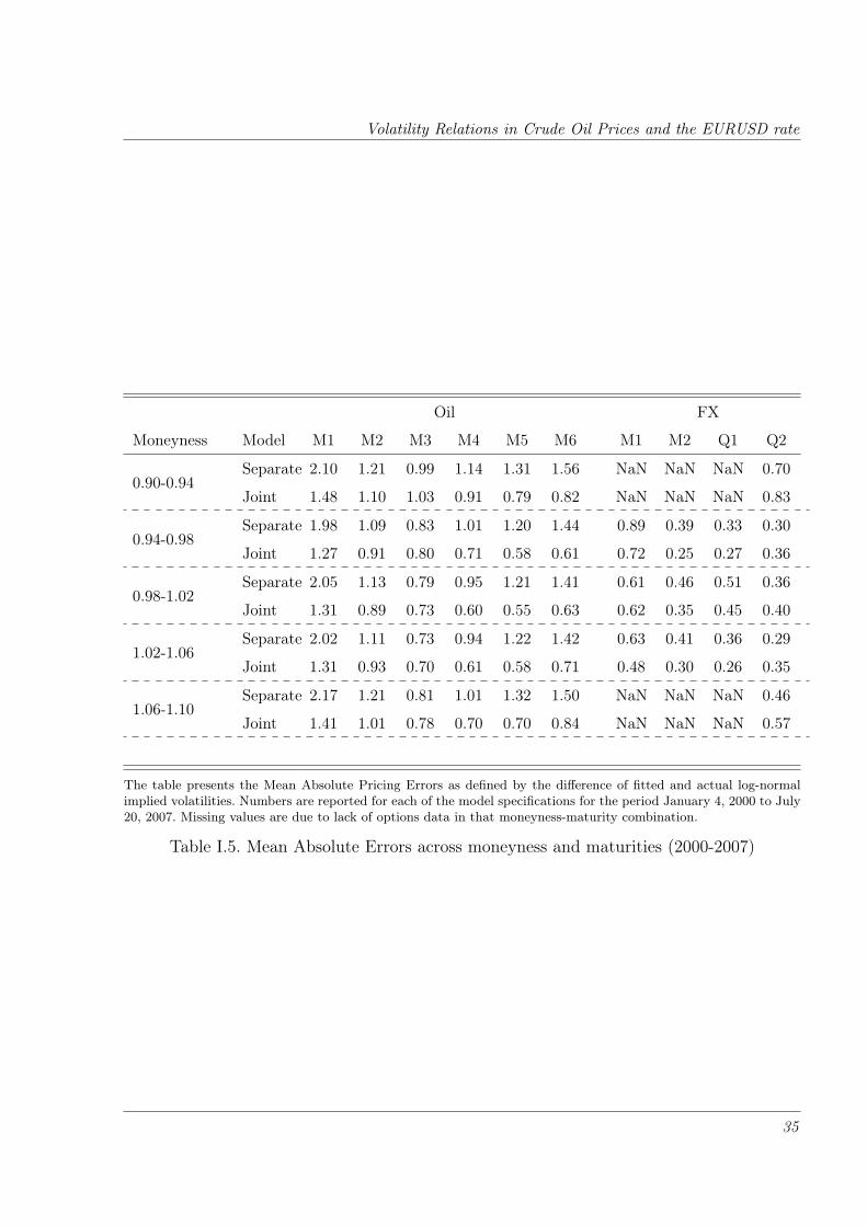
Volatility Relations in Crude Oil Prices and the EURUSD rate
Oil FX
Moneyness Model M1 M2 M3 M4 M5 M6 M1 M2 Q1 Q2
0.90-0.94Separate 2.10 1.21 0.99 1.14 1.31 1.56 NaN NaN NaN 0.70
Joint 1.48 1.10 1.03 0.91 0.79 0.82 NaN NaN NaN 0.83
0.94-0.98Separate 1.98 1.09 0.83 1.01 1.20 1.44 0.89 0.39 0.33 0.30
Joint 1.27 0.91 0.80 0.71 0.58 0.61 0.72 0.25 0.27 0.36
0.98-1.02Separate 2.05 1.13 0.79 0.95 1.21 1.41 0.61 0.46 0.51 0.36
Joint 1.31 0.89 0.73 0.60 0.55 0.63 0.62 0.35 0.45 0.40
1.02-1.06Separate 2.02 1.11 0.73 0.94 1.22 1.42 0.63 0.41 0.36 0.29
Joint 1.31 0.93 0.70 0.61 0.58 0.71 0.48 0.30 0.26 0.35
1.06-1.10Separate 2.17 1.21 0.81 1.01 1.32 1.50 NaN NaN NaN 0.46
Joint 1.41 1.01 0.78 0.70 0.70 0.84 NaN NaN NaN 0.57
The table presents the Mean Absolute Pricing Errors as defined by the difference of fitted and actual log-normalimplied volatilities. Numbers are reported for each of the model specifications for the period January 4, 2000 to July20, 2007. Missing values are due to lack of options data in that moneyness-maturity combination.
Table I.5. Mean Absolute Errors across moneyness and maturities (2000-2007)
35
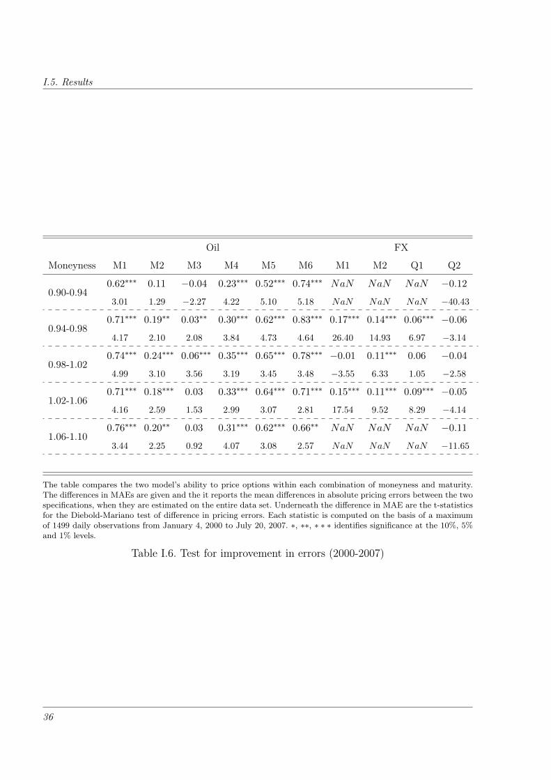
I.5. Results
Oil FX
Moneyness M1 M2 M3 M4 M5 M6 M1 M2 Q1 Q2
0.90-0.940.62∗∗∗ 0.11 −0.04 0.23∗∗∗ 0.52∗∗∗ 0.74∗∗∗ NaN NaN NaN −0.12
3.01 1.29 −2.27 4.22 5.10 5.18 NaN NaN NaN −40.43
0.94-0.980.71∗∗∗ 0.19∗∗ 0.03∗∗ 0.30∗∗∗ 0.62∗∗∗ 0.83∗∗∗ 0.17∗∗∗ 0.14∗∗∗ 0.06∗∗∗ −0.06
4.17 2.10 2.08 3.84 4.73 4.64 26.40 14.93 6.97 −3.14
0.98-1.020.74∗∗∗ 0.24∗∗∗ 0.06∗∗∗ 0.35∗∗∗ 0.65∗∗∗ 0.78∗∗∗ −0.01 0.11∗∗∗ 0.06 −0.04
4.99 3.10 3.56 3.19 3.45 3.48 −3.55 6.33 1.05 −2.58
1.02-1.060.71∗∗∗ 0.18∗∗∗ 0.03 0.33∗∗∗ 0.64∗∗∗ 0.71∗∗∗ 0.15∗∗∗ 0.11∗∗∗ 0.09∗∗∗ −0.05
4.16 2.59 1.53 2.99 3.07 2.81 17.54 9.52 8.29 −4.14
1.06-1.100.76∗∗∗ 0.20∗∗ 0.03 0.31∗∗∗ 0.62∗∗∗ 0.66∗∗ NaN NaN NaN −0.11
3.44 2.25 0.92 4.07 3.08 2.57 NaN NaN NaN −11.65
The table compares the two model’s ability to price options within each combination of moneyness and maturity.The differences in MAEs are given and the it reports the mean differences in absolute pricing errors between the twospecifications, when they are estimated on the entire data set. Underneath the difference in MAE are the t-statisticsfor the Diebold-Mariano test of difference in pricing errors. Each statistic is computed on the basis of a maximumof 1499 daily observations from January 4, 2000 to July 20, 2007. ∗, ∗∗, ∗ ∗ ∗ identifies significance at the 10%, 5%and 1% levels.
Table I.6. Test for improvement in errors (2000-2007)
36
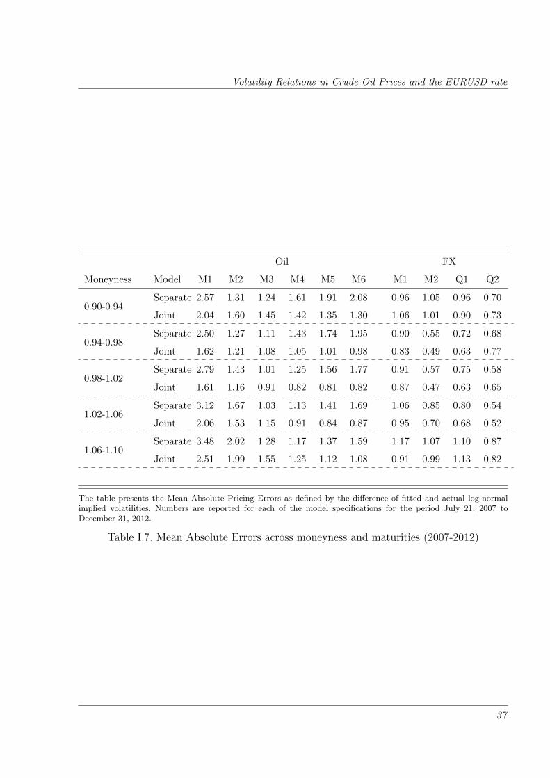
Volatility Relations in Crude Oil Prices and the EURUSD rate
Oil FX
Moneyness Model M1 M2 M3 M4 M5 M6 M1 M2 Q1 Q2
0.90-0.94Separate 2.57 1.31 1.24 1.61 1.91 2.08 0.96 1.05 0.96 0.70
Joint 2.04 1.60 1.45 1.42 1.35 1.30 1.06 1.01 0.90 0.73
0.94-0.98Separate 2.50 1.27 1.11 1.43 1.74 1.95 0.90 0.55 0.72 0.68
Joint 1.62 1.21 1.08 1.05 1.01 0.98 0.83 0.49 0.63 0.77
0.98-1.02Separate 2.79 1.43 1.01 1.25 1.56 1.77 0.91 0.57 0.75 0.58
Joint 1.61 1.16 0.91 0.82 0.81 0.82 0.87 0.47 0.63 0.65
1.02-1.06Separate 3.12 1.67 1.03 1.13 1.41 1.69 1.06 0.85 0.80 0.54
Joint 2.06 1.53 1.15 0.91 0.84 0.87 0.95 0.70 0.68 0.52
1.06-1.10Separate 3.48 2.02 1.28 1.17 1.37 1.59 1.17 1.07 1.10 0.87
Joint 2.51 1.99 1.55 1.25 1.12 1.08 0.91 0.99 1.13 0.82
The table presents the Mean Absolute Pricing Errors as defined by the difference of fitted and actual log-normalimplied volatilities. Numbers are reported for each of the model specifications for the period July 21, 2007 toDecember 31, 2012.
Table I.7. Mean Absolute Errors across moneyness and maturities (2007-2012)
37
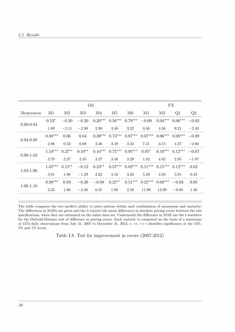
I.5. Results
Oil FX
Moneyness M1 M2 M3 M4 M5 M6 M1 M2 Q1 Q2
0.90-0.940.53∗ −0.30 −0.20 0.20∗∗∗ 0.56∗∗∗ 0.79∗∗∗ −0.09 0.04∗∗∗ 0.06∗∗∗ −0.03
1.89 −2.11 −2.90 2.90 3.46 3.22 0.46 4.56 9.21 −2.40
0.94-0.980.88∗∗∗ 0.06 0.04 0.39∗∗∗ 0.73∗∗∗ 0.97∗∗∗ 0.07∗∗∗ 0.06∗∗∗ 0.09∗∗∗ −0.09
2.86 0.23 0.68 3.36 3.49 3.34 7.21 3.15 4.27 −2.60
0.98-1.021.18∗∗∗ 0.27∗∗ 0.10∗∗ 0.44∗∗∗ 0.75∗∗∗ 0.95∗∗∗ 0.05∗ 0.10∗∗∗ 0.12∗∗∗ −0.07
3.79 2.37 2.45 3.27 3.48 3.29 1.82 4.82 2.95 −1.97
1.02-1.061.07∗∗∗ 0.15∗∗ −0.12 0.23∗∗ 0.57∗∗∗ 0.82∗∗∗ 0.11∗∗∗ 0.15∗∗∗ 0.12∗∗∗ 0.02
3.91 1.98 −1.29 2.23 3.16 3.20 5.29 4.94 5.01 0.45
1.06-1.100.98∗∗∗ 0.03 −0.26 −0.08 0.25∗∗ 0.51∗∗∗ 0.25∗∗∗ 0.08∗∗∗ −0.03 0.05
3.35 1.06 −2.30 0.31 1.98 2.58 11.98 14.99 −0.68 1.48
The table compares the two model’s ability to price options within each combination of moneyness and maturity.The differences in MAEs are given and the it reports the mean differences in absolute pricing errors between the twospecifications, when they are estimated on the entire data set. Underneath the difference in MAE are the t-statisticsfor the Diebold-Mariano test of difference in pricing errors. Each statistic is computed on the basis of a maximumof 1373 daily observations from July 21, 2007 to December 31, 2012. ∗, ∗∗, ∗ ∗ ∗ identifies significance at the 10%,5% and 1% levels.
Table I.8. Test for improvement in errors (2007-2012)
38
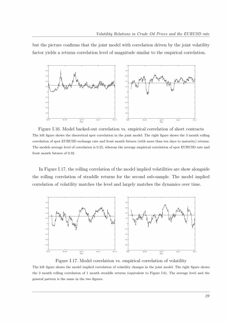
Volatility Relations in Crude Oil Prices and the EURUSD rate
but the picture confirms that the joint model with correlation driven by the joint volatility
factor yields a returns correlation level of magnitude similar to the empirical correlation.
Date
Jul-07 Dec-08 Apr-10 Aug-11 Dec-12-1
-0.8
-0.6
-0.4
-0.2
0
0.2
0.4
0.6
0.8
1
Date
Jul07 Dec08 Apr10 Aug11 Dec12-1
-0.8
-0.6
-0.4
-0.2
0
0.2
0.4
0.6
0.8
1
Figure I.16. Model backed-out correlation vs. empirical correlation of short contractsThe left figure shows the theoretical spot correlation in the joint model. The right figure shows the 3 month rolling
correlation of spot EURUSD exchange rate and front month futures (with more than ten days to maturity) returns.
The models average level of correlation is 0.25, whereas the average empirical correlation of spot EURUSD rate and
front month futures of 0.32.
In Figure I.17, the rolling correlation of the model implied volatilities are show alongside
the rolling correlation of straddle returns for the second sub-sample. The model implied
correlation of volatility matches the level and largely matches the dynamics over time.
Date
Jul-07 Dec-08 Apr-10 Aug-11 Dec-12-1
-0.8
-0.6
-0.4
-0.2
0
0.2
0.4
0.6
0.8
1
Date
Jul07 Dec08 Apr10 Aug11 Dec12-1
-0.8
-0.6
-0.4
-0.2
0
0.2
0.4
0.6
0.8
1
Figure I.17. Model correlation vs. empirical correlation of volatilityThe left figure shows the model implied correlation of volatility changes in the joint model. The right figure shows
the 3 month rolling correlation of 1 month straddle returns (equivalent to Figure I.6). The average level and the
general pattern is the same in the two figures.
39
I.6. Conclusion
I.6 Conclusion
Several studies argue that a change in the relationship between commodity markets and
financial markets has occurred after 2004 and other studies document a stronger relationship
during and after the financial crisis. In this paper, the correlation between the market
implied volatility in crude oil and the market implied volatility of the EURUSD rate has
been studied. Using first a model-free approach, straddle returns are computed for crude oil
and for EURUSD. The rolling correlation of short straddles increased in level around 2007.
A Principal Components Analysis showed that a the variation across straddles was driven
by joint factors in the period 2007-2012, but not in the period 2000-2007.
Using a term structure model for futures and options, a model including a joint volatility
factor is estimated. In line with the conclusions from the model free analysis, there is
improvement in options price fit for both oil options and EURUSD options for the period
2007-2012. When the same model was fitted to the period 2000-2007, the extra volatility
factor mainly served to improve the fit of oil options while leaving the fit of EURUSD
options largely unchanged.
Although the improvement in EURUSD options was not significant using a Diebold-
Mariano test, the fit was improved around 5% on average compared to the separate model.
Across moneyness and maturities, the fit was improved for EURUSD options on shorter
futures and the results could potentially be strengthened by using option surfaces of equal
size, such that an improvement in the fit of oil options is not over-emphasized compared to
an improvement in the fit of EURUSD options. Further the liquidity of the Q2-futures is
very low compared to the Q1-futures.
In this paper, there is no attempt to explain whether the relation between oil volatility
and EURUSD volatility is a crisis phenomenon or the result of financialization. My analysis
ends in 2012, which is not sufficiently long after the crisis to determine, if the volatility
relation is persistent. I leave the explanation of the existence of the joint volatility factor to
future research.
40
Volatility Relations in Crude Oil Prices and the EURUSD rate
Appendix
I.A Data Description
Figures I.18 and I.19 show the returns of the futures data. The magnitude of daily EURUSD
futures returns is much smaller than for oil futures. During the financial crisis, returns data
show more volatility. There is a large downwards spike in oil futures contracts at the 9/11
terrorist attack, but the event does not stand out in the EURUSD futures contracts.
Tables I.9 and I.10 shows the number of options after the initial sorting.During the 3260
trading days, oil options with an open interest of more than 100 contracts exists across all
moneyness-intervals and maturities, except for short out-of the money options and some
of the longer dated contracts. For EURUSD options on the other hand, there is limited
availability. For the M1, Q1 and Q2 contracts, almost all days have data for the ATM
options. For slightly OTM options, the three shortest maturities have prices up to 30%
of the time, whereas the Q2 contract have around 80% of the time. The choice of five
moneyness-intervals and six respectively four maturities was made in order to include a
reasonable option surface to represent market volatility across time and moneyness, while
at the same time ensuring that the number of options were not too uneven.
Tables I.11 and I.12 show the average implied volatility after the initial sorting. The
average value is between 0.30−0.55 for oil options and 0.10−0.30 for the EURUSD options.
As indicated from the returns plot, the implied volatility of oil is much higher for shorter
dated options. Further, a for each maturity a smirk is observed, i.e., the volatility for OTM
puts are higher than for OTM calls. The degree of the smirk is diminishing with increasing
time to maturity. The EURUSD implied ATM volatility is almost flat for all maturities,
but a bigger smile is seen for shorter dated options, although values for far OTM options
are based on very few observations and thereby not very good representation of the entire
period.
Tables I.13 and I.14 show the average option prices. As expected, OTM options are less
41

I.A. Data Description
expensive as are shorter dated options.
Finally, I.15 and I.16 shows the average open interest. The depth of the oil options
market is larger than that of the EURUSD market13. For oil options, the general picture is
that there are more open interest in OTM options than for ATM option. This is most likely
because options closer to a moneyness level of 1 could have been in the money (ITM) and
thereby being exercised prematurity. For FX options the picture is somewhat the same for
the middle moneyness intervals, but dips to low levels for the far OTM options. As very
few observations were available, the average open interest is not representative for OTM
options.
13It would be more correct to compare notional values, but as a EURUSD futures is for 125,000 EUR and an oil
futures is for 1,000 barrels of oil, the difference in value of contracts will not result in a similar depth market if
measured in value rather than number of contracts.
42
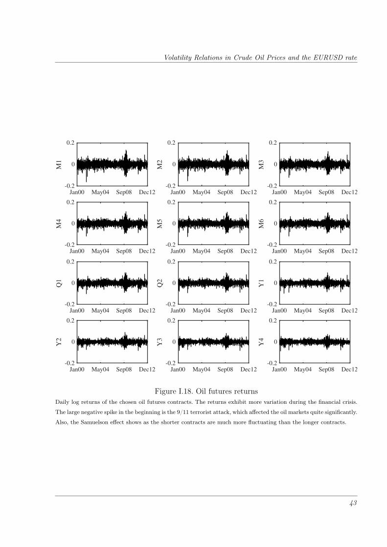
Volatility Relations in Crude Oil Prices and the EURUSD rate
Jan00 May04 Sep08 Dec12
M1
-0.2
0
0.2
Jan00 May04 Sep08 Dec12
M2
-0.2
0
0.2
Jan00 May04 Sep08 Dec12
M3
-0.2
0
0.2
Jan00 May04 Sep08 Dec12
M4
-0.2
0
0.2
Jan00 May04 Sep08 Dec12
M5
-0.2
0
0.2
Jan00 May04 Sep08 Dec12
M6
-0.2
0
0.2
Jan00 May04 Sep08 Dec12
Q1
-0.2
0
0.2
Jan00 May04 Sep08 Dec12
Q2
-0.2
0
0.2
Jan00 May04 Sep08 Dec12
Y1
-0.2
0
0.2
Jan00 May04 Sep08 Dec12
Y2
-0.2
0
0.2
Jan00 May04 Sep08 Dec12
Y3
-0.2
0
0.2
Jan00 May04 Sep08 Dec12
Y4
-0.2
0
0.2
Figure I.18. Oil futures returnsDaily log returns of the chosen oil futures contracts. The returns exhibit more variation during the financial crisis.
The large negative spike in the beginning is the 9/11 terrorist attack, which affected the oil markets quite significantly.
Also, the Samuelson effect shows as the shorter contracts are much more fluctuating than the longer contracts.
43
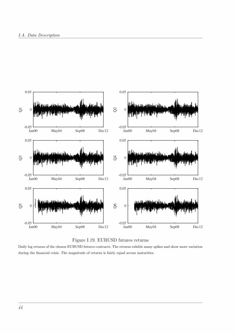
I.A. Data Description
Jan00 May04 Sep08 Dec12
Q1
-0.05
0
0.05
Jan00 May04 Sep08 Dec12
Q2
-0.05
0
0.05
Jan00 May04 Sep08 Dec12
Q3
-0.05
0
0.05
Jan00 May04 Sep08 Dec12
Q4
-0.05
0
0.05
Jan00 May04 Sep08 Dec12
Q5
-0.05
0
0.05
Jan00 May04 Sep08 Dec12
Q6
-0.05
0
0.05
Figure I.19. EURUSD futures returnsDaily log returns of the chosen EURUSD futures contracts. The returns exhibit many spikes and show more variation
during the financial crisis. The magnitude of returns is fairly equal across maturities.
44
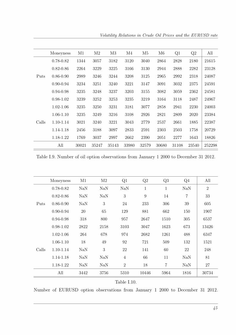
Volatility Relations in Crude Oil Prices and the EURUSD rate
Moneyness M1 M2 M3 M4 M5 M6 Q1 Q2 All
0.78-0.82 1344 3057 3182 3120 3040 2864 2828 2180 21615
0.82-0.86 2264 3229 3225 3166 3130 2944 2888 2282 23128
Puts 0.86-0.90 2989 3246 3244 3208 3125 2965 2992 2318 24087
0.90-0.94 3234 3251 3240 3221 3147 3091 3032 2375 24591
0.94-0.98 3235 3248 3237 3203 3155 3082 3059 2362 24581
0.98-1.02 3239 3252 3253 3235 3219 3164 3118 2487 24967
1.02-1.06 3235 3250 3231 3181 3077 2858 2941 2230 24003
1.06-1.10 3235 3249 3216 3108 2926 2821 2809 2020 23384
Calls 1.10-1.14 3021 3240 3221 3043 2779 2537 2661 1885 22387
1.14-1.18 2456 3188 3097 2833 2591 2303 2503 1758 20729
1.18-1.22 1769 3037 2997 2662 2390 2051 2277 1643 18826
All 30021 35247 35143 33980 32579 30680 31108 23540 252298
Table I.9. Number of oil option observations from January 1 2000 to December 31 2012.
Moneyness M1 M2 Q1 Q2 Q3 Q4 All
0.78-0.82 NaN NaN NaN 1 1 NaN 2
0.82-0.86 NaN NaN 3 9 14 7 33
Puts 0.86-0.90 NaN 3 24 233 306 39 605
0.90-0.94 20 65 129 881 662 150 1907
0.94-0.98 318 800 957 2647 1510 305 6537
0.98-1.02 2822 2158 3103 3047 1623 673 13426
1.02-1.06 264 678 974 2682 1261 488 6347
1.06-1.10 18 49 92 721 509 132 1521
Calls 1.10-1.14 NaN 3 22 141 60 22 248
1.14-1.18 NaN NaN 4 66 11 NaN 81
1.18-1.22 NaN NaN 2 18 7 NaN 27
All 3442 3756 5310 10446 5964 1816 30734
Table I.10.
Number of EURUSD option observations from January 1 2000 to December 31 2012.
45

I.A. Data Description
Moneyness M1 M2 M3 M4 M5 M6 Q1 Q2 All
0.78-0.82 0.53 0.43 0.41 0.39 0.38 0.37 0.36 0.34 0.39
0.82-0.86 0.47 0.42 0.40 0.38 0.37 0.36 0.35 0.34 0.38
Puts 0.86-0.90 0.43 0.40 0.39 0.38 0.36 0.35 0.34 0.33 0.38
0.90-0.94 0.41 0.39 0.38 0.37 0.36 0.35 0.34 0.32 0.37
0.94-0.98 0.39 0.38 0.37 0.36 0.35 0.34 0.33 0.31 0.36
0.98-1.02 0.38 0.37 0.36 0.35 0.35 0.34 0.32 0.31 0.35
1.02-1.06 0.38 0.37 0.36 0.35 0.34 0.33 0.32 0.31 0.35
1.06-1.10 0.38 0.37 0.36 0.35 0.34 0.33 0.32 0.31 0.35
Calls 1.10-1.14 0.39 0.37 0.36 0.35 0.34 0.33 0.32 0.31 0.35
1.14-1.18 0.41 0.37 0.36 0.35 0.34 0.33 0.32 0.30 0.35
1.18-1.22 0.44 0.38 0.37 0.36 0.35 0.34 0.32 0.31 0.36
All 0.41 0.39 0.37 0.36 0.35 0.34 0.33 0.32 0.36
Table I.11.
Average Implied Volatility of Oil Options from January 1 2000 to December 31 2012.
Moneyness M1 M2 Q1 Q2 Q3 Q4 All
0.78-0.82 NaN NaN NaN 0.28 0.20 NaN 0.24
0.82-0.86 NaN NaN 0.30 0.23 0.20 0.18 0.21
Puts 0.86-0.90 NaN 0.29 0.25 0.19 0.16 0.15 0.18
0.90-0.94 0.22 0.22 0.20 0.16 0.14 0.11 0.15
0.94-0.98 0.16 0.14 0.14 0.12 0.11 0.10 0.12
0.98-1.02 0.11 0.11 0.11 0.11 0.10 0.10 0.11
1.02-1.06 0.16 0.13 0.13 0.11 0.10 0.10 0.12
1.06-1.10 0.22 0.22 0.20 0.14 0.12 0.11 0.14
Calls 1.10-1.14 NaN 0.23 0.24 0.19 0.14 0.13 0.18
1.14-1.18 NaN NaN 0.28 0.21 0.18 NaN 0.21
1.18-1.22 NaN NaN 0.30 0.23 0.20 NaN 0.23
All 0.12 0.12 0.12 0.12 0.11 0.10 0.12
Table I.12.
Average Implied Volatility of EURUSD Options from January 1 2000 to December 31 2012.
46
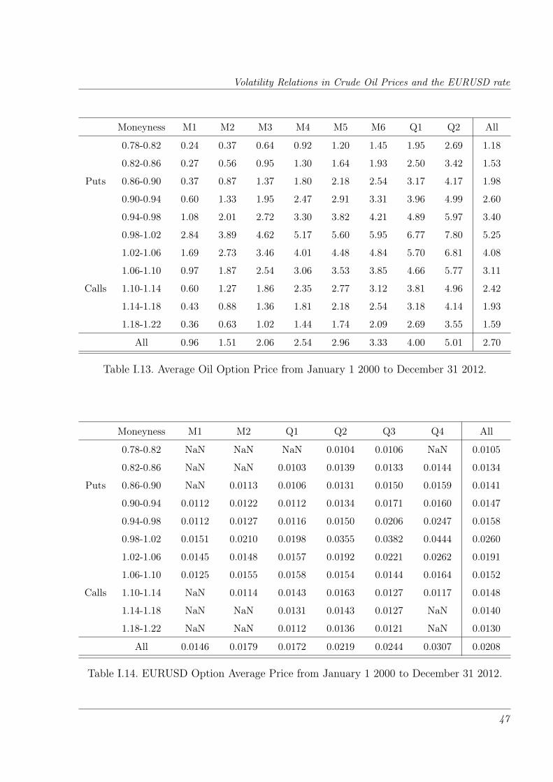
Volatility Relations in Crude Oil Prices and the EURUSD rate
Moneyness M1 M2 M3 M4 M5 M6 Q1 Q2 All
0.78-0.82 0.24 0.37 0.64 0.92 1.20 1.45 1.95 2.69 1.18
0.82-0.86 0.27 0.56 0.95 1.30 1.64 1.93 2.50 3.42 1.53
Puts 0.86-0.90 0.37 0.87 1.37 1.80 2.18 2.54 3.17 4.17 1.98
0.90-0.94 0.60 1.33 1.95 2.47 2.91 3.31 3.96 4.99 2.60
0.94-0.98 1.08 2.01 2.72 3.30 3.82 4.21 4.89 5.97 3.40
0.98-1.02 2.84 3.89 4.62 5.17 5.60 5.95 6.77 7.80 5.25
1.02-1.06 1.69 2.73 3.46 4.01 4.48 4.84 5.70 6.81 4.08
1.06-1.10 0.97 1.87 2.54 3.06 3.53 3.85 4.66 5.77 3.11
Calls 1.10-1.14 0.60 1.27 1.86 2.35 2.77 3.12 3.81 4.96 2.42
1.14-1.18 0.43 0.88 1.36 1.81 2.18 2.54 3.18 4.14 1.93
1.18-1.22 0.36 0.63 1.02 1.44 1.74 2.09 2.69 3.55 1.59
All 0.96 1.51 2.06 2.54 2.96 3.33 4.00 5.01 2.70
Table I.13. Average Oil Option Price from January 1 2000 to December 31 2012.
Moneyness M1 M2 Q1 Q2 Q3 Q4 All
0.78-0.82 NaN NaN NaN 0.0104 0.0106 NaN 0.0105
0.82-0.86 NaN NaN 0.0103 0.0139 0.0133 0.0144 0.0134
Puts 0.86-0.90 NaN 0.0113 0.0106 0.0131 0.0150 0.0159 0.0141
0.90-0.94 0.0112 0.0122 0.0112 0.0134 0.0171 0.0160 0.0147
0.94-0.98 0.0112 0.0127 0.0116 0.0150 0.0206 0.0247 0.0158
0.98-1.02 0.0151 0.0210 0.0198 0.0355 0.0382 0.0444 0.0260
1.02-1.06 0.0145 0.0148 0.0157 0.0192 0.0221 0.0262 0.0191
1.06-1.10 0.0125 0.0155 0.0158 0.0154 0.0144 0.0164 0.0152
Calls 1.10-1.14 NaN 0.0114 0.0143 0.0163 0.0127 0.0117 0.0148
1.14-1.18 NaN NaN 0.0131 0.0143 0.0127 NaN 0.0140
1.18-1.22 NaN NaN 0.0112 0.0136 0.0121 NaN 0.0130
All 0.0146 0.0179 0.0172 0.0219 0.0244 0.0307 0.0208
Table I.14. EURUSD Option Average Price from January 1 2000 to December 31 2012.
47
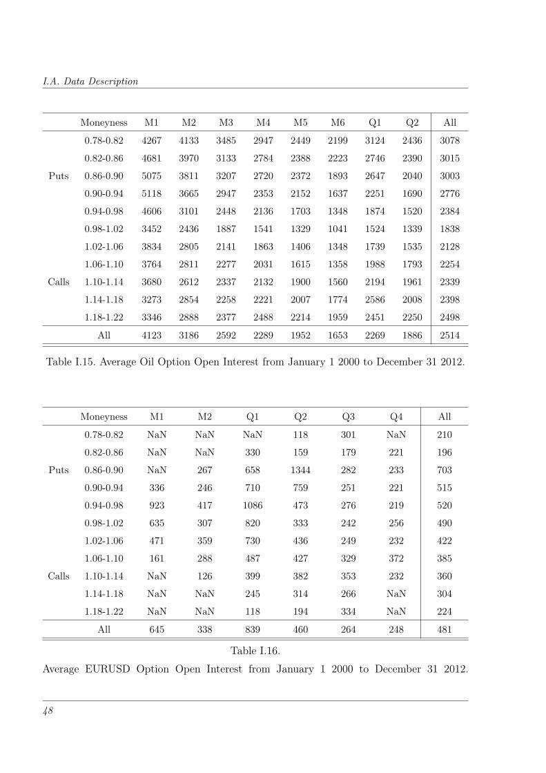
I.A. Data Description
Moneyness M1 M2 M3 M4 M5 M6 Q1 Q2 All
0.78-0.82 4267 4133 3485 2947 2449 2199 3124 2436 3078
0.82-0.86 4681 3970 3133 2784 2388 2223 2746 2390 3015
Puts 0.86-0.90 5075 3811 3207 2720 2372 1893 2647 2040 3003
0.90-0.94 5118 3665 2947 2353 2152 1637 2251 1690 2776
0.94-0.98 4606 3101 2448 2136 1703 1348 1874 1520 2384
0.98-1.02 3452 2436 1887 1541 1329 1041 1524 1339 1838
1.02-1.06 3834 2805 2141 1863 1406 1348 1739 1535 2128
1.06-1.10 3764 2811 2277 2031 1615 1358 1988 1793 2254
Calls 1.10-1.14 3680 2612 2337 2132 1900 1560 2194 1961 2339
1.14-1.18 3273 2854 2258 2221 2007 1774 2586 2008 2398
1.18-1.22 3346 2888 2377 2488 2214 1959 2451 2250 2498
All 4123 3186 2592 2289 1952 1653 2269 1886 2514
Table I.15. Average Oil Option Open Interest from January 1 2000 to December 31 2012.
Moneyness M1 M2 Q1 Q2 Q3 Q4 All
0.78-0.82 NaN NaN NaN 118 301 NaN 210
0.82-0.86 NaN NaN 330 159 179 221 196
Puts 0.86-0.90 NaN 267 658 1344 282 233 703
0.90-0.94 336 246 710 759 251 221 515
0.94-0.98 923 417 1086 473 276 219 520
0.98-1.02 635 307 820 333 242 256 490
1.02-1.06 471 359 730 436 249 232 422
1.06-1.10 161 288 487 427 329 372 385
Calls 1.10-1.14 NaN 126 399 382 353 232 360
1.14-1.18 NaN NaN 245 314 266 NaN 304
1.18-1.22 NaN NaN 118 194 334 NaN 224
All 645 338 839 460 264 248 481
Table I.16.
Average EURUSD Option Open Interest from January 1 2000 to December 31 2012.
48
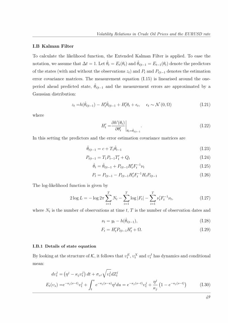
Volatility Relations in Crude Oil Prices and the EURUSD rate
I.B Kalman Filter
To calculate the likelihood function, the Extended Kalman Filter is applied. To ease the
notation, we assume that ∆t = 1. Let θt = Et(θt) and θt|t−1 = Et−1(θt) denote the predictors
of the states (with and without the observations zt) and Pt and Pt|t−1 denotes the estimation
error covariance matrices. The measurement equation (I.15) is linearised around the one-
period ahead predicted state, θt|t−1 and the measurement errors are approximated by a
Gaussian distribution:
zt =h(θt|t−1)−H ′tθt|t−1 +H ′tθt + εt, εt ∼ N (0, Ω) (I.21)
where
H ′t =∂h′(θt)
∂θ′t
∣∣∣∣θt=θt|t−1
. (I.22)
In this setting the predictors and the error estimation covariance matrices are
θt|t−1 = c+ T1θt−1 (I.23)
Pt|t−1 = T1Pt−1T′1 +Qt (I.24)
θt = θt|t−1 + Pt|t−1H′tF−1t νt (I.25)
Pt = Pt|t−1 − Pt|t−1H′tF−1t HtPt|t−1 (I.26)
The log-likelihood function is given by
2 logL = − log 2πT∑i=1
Nt −T∑i=1
log |Ft| −T∑i=1
ν ′tF−1t νt, (I.27)
where Nt is the number of observations at time t, T is the number of observation dates and
νt = yt − h(θt|t−1), (I.28)
Ft = H ′tPt|t−1H′t + Ω. (I.29)
I.B.1 Details of state equation
By looking at the structure of K, it follows that υEt , υXt and υJt has dynamics and conditional
mean:
dυjt =(ηj − κjυjt
)dt+ συj
√υjtdZ
jt
Et(υs) =e−κj(s−t)υjt +
∫ s
t
e−κj(s−u)ηjdu = e−κj(s−t)υjt +ηj
κj
(1− e−κj(s−t)
)(I.30)
49

I.B. Kalman Filter
Using (I.9), (I.10), (I.11), (I.5), and (I.6), the state equations’ terms are collected:
dθt = (Φ−Kθt) dt+√υEt RE
dWE
t
dBEt
dZEt
+√υXt RX
dWX
t
dBXt
dZXt
+√υJt RJ
(dW J
t
dZJt
), (I.31)
where the R-terms are matrices consisting of 0’s, 1’s and σ’s.
The conditional mean of θt+∆t given θt is:
Et(θt+∆t) = e−K∆t︸ ︷︷ ︸T∆t
θt + e−K∆t
∫ ∆t
0
eKudu · Φ︸ ︷︷ ︸c∆t
(I.32)
Both T∆t and c∆t are easily computed. The conditional covariance of θt has the following
form
Covt(θt+∆t) = Q0 +QEυEt +QXυXt +QJυJt
and is given by:
Covt(θt+∆t) =
[∫ t+∆t
t
Et(υEu)e−K(t+∆t−u)REΣER
′Ee−K′(t+∆t−u)du
]+
[∫ t+∆t
t
Et(υXu)e−K(t+∆t−u)RXΣXR
′Xe−K′(t+∆t−u)du
]+
[∫ t+∆t
t
e−K(t+∆t−u)RJΣJR′Je−K′(t+∆t−u)du
]=υEt
[∫ t+∆t
t
e−κE(u−t)e−K(t+∆t−u)REΣER′Ee−K′(t+∆t−u)du
]+ υXt
[∫ t+∆t
t
e−κX(u−t)e−K(t+∆t−u)RXΣXR′Xe−K′(t+∆t−u)du
]+ υJt
[∫ t+∆t
t
e−κJ (u−t)e−K(t+∆t−u)RJΣJR′Je−K′(t+∆t−u)du
]+
[∫ t+∆t
t
ηE
κE
(1− e−κE(u−t)) e−K(t+∆t−u)REΣER
′Ee−K′(t+∆t−u)du
]+
[∫ t+∆t
t
ηX
κX
(1− e−κX(u−t)) e−K(t+∆t−u)RXΣXR
′Xe−K′(t+∆t−u)du
]+
[∫ t+∆t
t
ηJ
κJ
(1− e−κJ (u−t)) e−K(t+∆t−u)RJΣJR
′Je−K′(t+∆t−u)du
]where Σj is the covariance matrices for the Brownian motions.
50
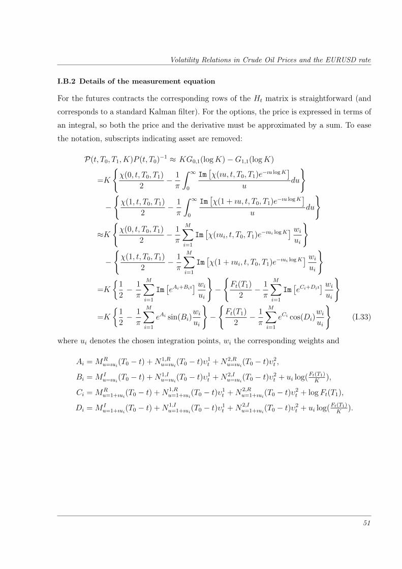
Volatility Relations in Crude Oil Prices and the EURUSD rate
I.B.2 Details of the measurement equation
For the futures contracts the corresponding rows of the Ht matrix is straightforward (and
corresponds to a standard Kalman filter). For the options, the price is expressed in terms of
an integral, so both the price and the derivative must be approximated by a sum. To ease
the notation, subscripts indicating asset are removed:
P(t,T0,T1,K)P (t,T0)−1 ≈ KG0,1(logK)−G1,1(logK)
=K
χ(0, t,T0,T1)
2− 1
π
∫ ∞0
Im[χ(ıu, t,T0,T1)e−ıu logK
]u
du
−
χ(1, t,T0,T1)
2− 1
π
∫ ∞0
Im[χ(1 + ıu, t,T0,T1)e−ıu logK
]u
du
≈K
χ(0, t,T0,T1)
2− 1
π
M∑i=1
Im[χ(ıui, t,T0,T1)e−ıui logK
] wiui
−
χ(1, t,T0,T1)
2− 1
π
M∑i=1
Im[χ(1 + ıui, t,T0,T1)e−ıui logK
] wiui
=K
1
2− 1
π
M∑i=1
Im[eAi+Biı
] wiui
−
Ft(T1)
2− 1
π
M∑i=1
Im[eCi+Diı
] wiui
=K
1
2− 1
π
M∑i=1
eAi sin(Bi)wiui
−
Ft(T1)
2− 1
π
M∑i=1
eCi cos(Di)wiui
(I.33)
where ui denotes the chosen integration points, wi the corresponding weights and
Ai = MRu=ıui
(T0 − t) +N1,Ru=ıui
(T0 − t)υ1t +N2,R
u=ıui(T0 − t)υ2
t ,
Bi = M Iu=ıui
(T0 − t) +N1,Iu=ıui
(T0 − t)υ1t +N2,I
u=ıui(T0 − t)υ2
t + ui log(Ft(T1)K
),
Ci = MRu=1+ıui
(T0 − t) +N1,Ru=1+ıui
(T0 − t)υ1t +N2,R
u=1+ıui(T0 − t)υ2
t + logFt(T1),
Di = M Iu=1+ıui
(T0 − t) +N1,Iu=1+ıui
(T0 − t)υ1t +N2,I
u=1+ıui(T0 − t)υ2
t + ui log(Ft(T1)K
).
51


How Energy Quanto Options can Hedge Volumetric Risk
Essay II
How Energy Quanto Options can Hedge Volumetric
Risk∗
Abstract
Many corporations do not have full control over the quantities they sell or purchase
and at which price. Their operation therefore includes volumetric risk and in most
cases the volumetric risk is not tradable, and sufficient management of risk can thus
be difficult to obtain. But when the quantity is closely related to another tradable
asset, risk management strategies based on both prices and the correlated asset
shows to be superior compared to hedges based on only the price. Although it
can be derived for very simple frameworks, closed form solutions for the optimal
hedge are not available for the general case. But when a closed form solution is
available, the theoretical hedge is not a straightforward function of price and the
other traded asset, so finding a counterpart can be difficult. This paper shows that
energy quanto options arises naturally in any optimal trading strategy. Through
a comparative study, it is shown that a hedge using just one or two energy
quanto options do remarkably well compared to the theoretical optimal hedge.
The comparative study further illustrates that the choice of energy quanto options
depends on the behaviour of the underlying variables.
∗I thank Fred Espen Benth, Glen Swindle, Søren Feodor Nielsen and Peter Lyk-Jensen for helpful discussions.
53
II.1. Introduction
II.1 Introduction
Producers and consumers of energy are facing several types of risks. Two key uncertainties
are the quantity sold or purchased and the market price. Some businesses might have the
option to adjust the quantity in response to the price, but a farmer, a wind park owner or
a provider of energy must in many situations just accept both the market price and the
quantity produced or demanded. For instance, in the retail and wholesale markets for gas
and electricity, typical contracts allows the costumer to consume as much gas or electricity
as needed at a pre-determined fixed rate. E.g., for electricity the fixed rate could be set on a
monthly, quarterly or annual basis. For the consumer, the only uncertainty faced is therefore
the quantity she uses. If the paid rate is not sufficient to cover the purchase or production
of her electricity, she is not financially punished nor is she rewarded, if prices are lower
than the agreed rate. The provider of electricity – often denoted as the Load Serving Entity
(LSE) – faces all the price risk and this price risk is potentially amplified by the uncertainty
in demanded quantity. The positive relationship between prices and consumption leads the
following stylized problem: When demand is high, the price of electricity is also high, leading
to a negative profit margin multiplied with a high quantity, i.e., a loss for the LSE. When
quantity and thereby prices are low, the profit margin might be positive, but when selling
a low quantity, the revenue for the LSE is low.
The reasons for engaging in risk managements are many and the topic has been addressed
frequently in the literature. Without addressing the particular reasons a company might have
for hedging certain risks, the focus in this paper is how to hedge the risk. The same approach
was used in Brown and Toft (2002), who take as given a non-financial firm that hedges using
derivatives contracts and focus on the design of an appropriate hedge strategy based on the
future price without specifying the functional form of the hedge. Contrary to many other
papers, they refrain from assuming that the hedge is made up of e.g., forwards or futures
and options, but derive the ”perfect exotic hedge”. They study this in a simple set-up, where
a company produces an uncertain quantity of a single good, which is sold at an uncertain
price. The company is value-maximizing and faces a deadweight cost, which gives them
incentives to hedge. Their derived perfect exotic hedge depends on the correlation between
the price and quantity as well as the uncertainty in these together with the risk-aversion
as represented in the deadweight costs. This enables the company to hedge some of the
otherwise unhedgeable quantity risk by exploiting the correlation of price and quantity.
54

How Energy Quanto Options can Hedge Volumetric Risk
This approach has been studied in the context of energy markets and the related
literature is discussed in more detailed in Section II.2. The challenge when hedging quantity
risk is that contrary to the market price risk, there are no derivatives contracts available
to target the quantity risk1 resulting in an incomplete market as long as the correlation is
imperfect. But as the link between quantity and weather is well-established for commodity
markets (although the nature of this relationship differs across markets and locations
depending on the type of commodity considered), a natural extension is to let the perfect
hedge depend on not only the price, but also a weather-related index on which financial
contracts exist. Id Brik and Roncoroni (2016a) generalise the idea of a perfect exotic hedge
to two dimensions and let the hedge be a general function of underlying price and an index
that correlates with quantity. The major problem is however, that the hedge strategy has a
functional form that depends on density ratios and the conditional mean of the unhedged
profit. For some distributional assumptions, the functional form of the hedge is available in
closed form, but even for simple settings like the (log-)normal distribution, the functional
form is not a straightforward expression. In practice, it would be difficult to approach a
counterpart and ask for a such structured deal.
The issue of quantity risk is widely present in agricultural markets. A farmer’s unhedged
revenue is the quantity at harvest time times the price earned for the quality of corn he
produces. Setting aside basis risk, the farmer is exposed to the product of two negatively
correlated variables. If total crop production is high, there is generally an over-supply in the
market which affects prices negatively and vice versa2. The farmer is concerned about low
revenue, i.e., that the quantity times price is low3. In stylized terms, the risk management
problem for the LSE is similar to the risk management problem of farmer making the
solutions proposed in the agricultural finance literature relevant to relate to energy markets.
The focus of this paper is to show that energy quanto options – also sometimes referred
to as double structure options, double trigger options or weather cross-commodity options –
are strong alternatives to the perfect exotic hedge, when engaging in a hedge with an over-
1Futures contracts related to quantities in the agricultural markets were traded on CBOT during the 90s, but was
shortly after introduction delisted again because of low interest.2In real life, basis risk plays a major role as the individual farmer’s production might not correlate with total crop
production and he might face locational spreads in the price.3The risk management problem of the farmer is basically equivalent to that of the LSE. Using the notation introduced
in Section II.3, let St = R−Pt. The LSE is then worried about low StQt, where St and Qt are negatively correlated,
as Pt and Qt were positively correlated.
55
II.2. Background and related literature
the-counter counterpart. Counterparts in such a deal could for instance be re-insurance
companies4. For a general hedge strategy expressed as a function of two underlyings, the
replication result in Carr and Madan (2001) is extended to two dimensions and energy
quanto options arise as a natural part of the perfect exotic hedge. Following this, a
comparative simulation study is done to show that hedges using just one or two energy
quanto option perform remarkably well compared to the perfect exotic hedge as proposed
by Id Brik and Roncoroni (2016a).
The paper continues as follows: In Section II.2, literature related to dealing with quantity
risk is discussed. In Section II.3, the general risk management problem is presented and then
simplified to a one-period setting. It is shown that energy quanto options arises in the perfect
exotic hedge. Section II.4 contains a simulation study that compares hedges using energy
quanto hedge strategies with other both customized and market available strategies. Section
II.5 rounds off the paper including a discussion of further analyses.
II.2 Background and related literature
The application of the approach proposed by Brown and Toft (2002) to energy markets
was first done by Oum and Oren (2006). Where Brown and Toft (2002) use an assumption
of normally distributed price and quantity and employ maximization of profits net of dead
weight costs5, Oum and Oren (2006) solve the hedging problem for a general utility function
and separate probability functions for the physical measure and the risk-neutral pricing
measure. For a CARA utility function and for a mean-variance approach, the customized
hedge can be expressed in terms of the two densities and functions hereof. For the mean-
variance approach, the hedge from Oum and Oren (2006) hedge is later presented as Strategy
II.3. They illustrate the results of their model for a log-normal price and both normal and
log-normal quantity. They discuss the replication using forwards and options and in the
later paper, Oum and Oren (2010), the discretization error of the replicating strategy as
well as when to optimally enter the hedge is analysed. Also, Näsäkkälä and Keppo (2005)
4As an example, Munich Re mentions this type of contracts in their Topics Risk Insurance in 2014 (see Munich Re
(2014)). On http://www.swissre.com/corporate_solutions/weather_risk_solutions_double_trigger.html, Swiss Re
also mentions these type of products. Eydeland and Wolyniec (2003) describes this type of options as well under the
title Synthetic Peaker.5Korn (2009) later relaxes the assumption of normality and shows that the optimal payoff function takes different
forms arising from the assumed dependence structure rather than being a second order polynomial in price
56
How Energy Quanto Options can Hedge Volumetric Risk
analyse the timing issue, when only using forward contracts.
Several studies demonstrate the link between quantity and weather, e.g., Engle et al.
(1992), Timmer and Lamb (2007) and Swindle (2014), making the next natural step to
include weather contracts in the above-mentioned strategies. While not presenting the
details, Eydeland and Wolyniec (2003) study the efficiency of weather hedges by looking at
the residual cash flow. For electricity markets, they argue that weather hedges do not add
much value after application of a price hedge, whereas for gas markets it can be worthwhile
to consider basing the hedge on weather contracts.
Lee and Oren (2009) introduce an equilibrium economy, where market participants can
invest in a customized hedge based on the energy price and a weather contract whose
price is determined by supply and demand in the economy rather than being priced under
an exogenously given pricing measure. Id Brik and Roncoroni (2016b) and Id Brik and
Roncoroni (2016a) extend the customized hedge to be a general function of price and a linked
index. The former paper employs a customized hedge which is the sum of a general function
of price and a general function of the linked index and derive closed form solutions under the
assumption that price and index is independent, while price-quantity and quantity-index are
correlated. The latter paper views the customized hedge as a general function of price and
index. The exact functional form of the hedge depends on the underlying joint distribution
of price, quantity and index. An assumption of log-normality will for instance result in a
functional form that partly depends on the product of price and index raised to various
powers.
In the agricultural finance literature, a similar development in hedge strategies are seen.
Papers analysing hedges based on prices only, e.g., Moschini and Lapan (1995). They
conclude that options are needed to hedge the joint production and price risk. When
standardized yield futures was introduced in 1995 on the Chicago Board of Trade, a tool
was provided for managing the quantity risk directly rather than through the correlation
of price and quantity. Aase (2004) develops a pricing model for combined price futures and
yield futures, which can price contracts depending on both underlying and further points
out that (a synthetic) revenue futures can be obtained via dynamic trading in underlying
futures under the assumption of no basis risk and no transactions costs. The yield futures
contracts were de-listed shortly after introduction due to low trading interest.
Lien and Hennessy (2004) compare revenue futures to price futures and highlight the
trade-off in contract design: To ensure market depth, a revenue futures contract must be
57

II.2. Background and related literature
based on a broad geographical area. But at the same time this will lead to high idiosyncratic
risk making the hedge inefficient compared to a pure price hedge. As also pointed out by
Poitras (2013), the source of uncertainty that a farmer needs to insure is the income, rather
than the quantity and price components of the income. There seems to be little need for
construction of revenue futures or yield futures in the North America, as crop insurance
products are administered and state subsidized. Since 1996, specific revenue insurance
contract have been available. Cornaggia (2013) points out that the use of insurance can
further be attributed to pure risk management, whereas the use of derivatives could also be
a sign of speculation. In conclusion, although a farmer generally faces the same type of risk
management problems as an energy company, there has been a strong development towards
a state-subsidized solution in terms of crop insurance programs6.
In most of the papers referred to above, the focus is on a one-period static hedging
problem is studied. While this is fairly realistic when risk managing crop production, where
harvest is an annual or bi-annual occurrence, the risk management problem becomes more
complex for energy markets as the owner of a wind farm or a LSE are selling or buying
different quantities of power at different hourly rates. The profit or revenue will therefore
be a sum of products of hourly quantities and prices. The available market traded contracts
are on the other hand energy forwards, i.e., depending on the average price over a period,
for instance a month, a quarter or all peak-hours in a given week, energy options written on
the forwards and index futures on an accumulated index over a calender month. Kleindorfer
and Li (2005) analyse a multi-period framework by imposing a regularity condition on the
distribution of cash flows and illustrate results for the PJM market. In general, it is not
possible to derive an expression for an optimal hedge in a multi-period framework. A second
issue that an LSE should be consider is the portfolio effect. Most LSE also holds generation
power and the risks from generation of power should not be isolated from the risk arising
from providing power to end-customers.
Another issue which is seem not to have been addressed is the peculiar relationship
between price and quantity. As pointed out in e.g., Eydeland and Wolyniec (2003), the
price and demanded quantity have a strong relationship for low and medium prices, while it
breaks down for high prices. When closed form hedge strategies are solved, the assumptions
made regarding the price-quantity correlation in most studies does not incorporate this
6The fact that so many farmers use insurance could indicate that farmers are risk averse as a low revenue in one
season can have severe consequences for the future of their business.
58

How Energy Quanto Options can Hedge Volumetric Risk
feature. If hedge strategies are analysed with real data rather than in a stylized market,
this should be addressed using the exact characteristics of the market in question. In this
paper, the use of the OTC market for structuring tailor made hedges is promoted. However,
the classic trade-off of credit risk vs. basis risk when deciding between OTC structured
derivatives and market traded contracts should be taken into consideration. In many cases,
the availability of market traded contracts is so limited that an OTC contract provide a
strong alternative to market based hedges due to the basis risk and the liquidity premium
in the latter. Golden et al. (2007) analyses this trade-off in a one period model without price
risk.
On a final note, alternatives to risk management using derivatives should mentioned. The
LSE could pass on their price risk to the customer by charging the actual spot price (plus
a profit margin). This could be based one real-time data, but requireds the technology to
read off the consumption in real time as well as provide price information to the consumers
to which they can adjust to in an either automated or manual way. For instance, Pacific
Northwest GridWise Demonstration Project saw a decrease in peak loads (in which case
the price and quantity have more a complex relationship) as well as a decrease in the
average electricity bill7. This way of handling the profit risk is arguably an initiative that
has more merits in the context of grid reliability, and potential risk management benefits
should more be seen as the bi-product. A simpler approach to transfer of the price risk
is to charge customers the actual average costs per unit consumed8. For instance, in 2015
the default contract for a customer in the Danish energy company DONG Energy changed
from quarterly fixed rates to monthly rates based on the actual costs (including balancing
and trading costs) for purchase of power on Nord Pool, while at the same time raising the
monthly subscription.
Although these spot based contract structures, whether they are hourly or average based,
are becoming increasingly available in some markets, the fixed rate contract is still a widely
used contract. For the rest of this paper, we continue the string of literature considering the
hedging problem an LSE faces when offering fixed rate contracts.
7https://www.smartgrid.gov/files/GridWise_Demonstration_Project_Fast_Facts_200708.pdf8Or weighted according to a pre-determined template.
59
II.3. Risk management problem for an energy retailer
II.3 Risk management problem for an energy retailer
In this section, the risk management problem is presented in a general form and subsequently
simplified to a one-period static hedging problem. As discussed in the previous section,
many solutions to the simple hedging problem have been proposed in the literature and
the resulting strategies are presented in Section II.4.1. Using the solution in Id Brik and
Roncoroni (2016a) combined with the representation result proposed by Carr and Madan
(2001), energy quanto contracts arise naturally as a part of the customized hedge.
II.3.1 The general profit expression
Consider an energy retailer who charges a fixed price of R over the time horizon [0,T ].
Before hedging, the profit and loss for an energy retailer over this period is
V[0,T ] =
∫ T
0
e−rtt(R− Pt)Qtdt (II.1)
where Qt is the amount of energy delivered to customers at time t and Pt the corresponding
price. In practice, the price Pt and the demanded quantity Qt are piece-wise linear functions.
I.e., if the retailer is facing n prices per year, the profit and loss will be
V[0,T ] =nT∑j=1
e−rtj tj(R− Ptj)Qtj (II.2)
where tj = jn. If T is measured in years, setting n = 365 corresponds to daily prices and
n = 24×365 corresponds to hourly prices. rtj ,Ptj and Qtj are the interest, price and quantity
faced over the period [tj−1, tj].
II.3.2 Structuring of hedge contract
In the most simple case n = T = 1. This is the case of delivery of an uncertain amount of
energy Q at an unknown price P . Further, it is assumed that there exists an index I on
which contracts can be written and that the volume Q is correlated with this index. The
main question is then; if it is possible to structure a payoff depending on price P and this
index I, what is then the optimal structure? The value after entering such a hedge would
be: Vh = Q(R− P ) + x(P , I)9. The optimal hedge choice can mathematically be expressed
9The condition in II.3 ensures that the cost of the hedge in included in the structure of x.
60
How Energy Quanto Options can Hedge Volumetric Risk
as the solution to:
maxx(p,i)
E(U(Vh)) s.t. EQ(x(P , I)) = 0 (II.3)
where U is a utility function. The solution to this problem x∗(p, i) is a function of p and i and
depends on the choice of utility function as well as the distribution of P , Q and I under the
physical probability measure and the distribution of P and I under a risk-neutral measure.
This is the main result in Id Brik and Roncoroni (2016a), who also gives the functional form
for a generalised mean-variance utility function. In Proposition II.2, the general functional
form of the hedge is replicated using various contracts. It is a straightforward extension of
the one-dimensional version from by Carr and Madan (2001), which is stated below:
Lemma II.1 (Carr and Madan (2001)) Any twice differentiable function x : R → Rcan be represented as
x(p) =x(FP ) + x′(FP )(p− FP ) +
∫ FP
0
x′′(K)(K − p)+dK +
∫ ∞FP
x′′(K)(p−K)+dK
If the customized hedge x is only a function of the price, the formula shows that customized
hedge can be replicated in terms of a combination of a bank account, a forward contract,
a continuum of put options with strike smaller than the forward price and a continuum of
call options with strike larger than the forward price10. In reality, the customized hedge can
only be approximated by a finite number of options as not all strikes are available.
Proposition II.2 Any bivariate function x : R2 → R that is twice differentiable in both
arguments can be represented as
x(p, i) = x(FP ,FI) (II.4)
+ xi(FP ,FI)(i− FI) + xp(FP ,FI)(p− FP ) (II.5)
+ xpi(FP ,FI) ((i− FI)(p− FI)) (II.6)
+
∫ FI
0
xii(FP ,M)(M − i)+dM +
∫ ∞FI
xii(FP ,M)(i−M)+dM (II.7)
+
∫ FP
0
xpp(K,FI)(K − p)+dK +
∫ ∞F
xpp(K,FI)(p−K)+dK (II.8)
+ (p− FP )
∫ FI
0
xpii(FP ,M)(M − i)+dM (II.9)
10The expansion does not have to be around the current forward price FP , but this choice makes the most economic
sense because the second term then equals the payoff of x′(FP ) forward contracts.
61

II.3. Risk management problem for an energy retailer
+ (p− FP )
∫ ∞FI
xpii(FP ,M)(i−M)+dM (II.10)
+ (i− FI)∫ FP
0
xppi(K,FI)(K − p)+dK (II.11)
+ (i− FI)∫ ∞FP
xppi(K,FI)(p−K)+dK (II.12)
+
∫ FP
0
∫ ∞FI
xppii(K,M)(i−M)+(K − p)+dMdK (II.13)
+
∫ FP
0
∫ FI
0
xppii(K,M)(M − i)+(K − p)+dMdK (II.14)
+
∫ ∞FP
∫ FI
0
xppii(K,M)(M − i)+(p−K)+dMdK (II.15)
+
∫ ∞FP
∫ ∞FI
xppii(K,M)(i−M)+(p−K)+dMdK (II.16)
where subscripts denote differentiation with respect to the function arguments. This result
states that the optimal hedge consists of several different contract types:
• (II.4): bank account
• (II.5): forward/future on energy and the index
• (II.6): energy quanto swap11
• (II.7): continuum of options on the index
• (II.8): continuum of options on energy
• (II.9)-(II.12): the product of a forward and a continumm of options12
• (II.13)-(II.16): continuum of energy quanto options 2
The proposition states that the customized hedge can be replicated using the contract types
listed above, one of which is the energy quanto option. The importance of a specific type of
contract is given by the value of various derivatives of the customized hedge. For the simple
model in Id Brik and Roncoroni (2016a), it would be possible to derive and analyse the shape
of these quantities and for instance analyse the discretisation error as done by Oum and Oren
11Energy quanto swaps are also studied in Cucu et al. (2016)12These terms can also be expressed as a continuum of regular quanto options net of a continuum of univariate
options.
62

How Energy Quanto Options can Hedge Volumetric Risk
(2010). But as the counterpart for an energy quanto option is found in the OTC market,
buying (or selling if the derivatives of x∗ is negative) multiple energy quanto options would
be an expensive strategy in practice. Instead, Proposition II.2 is used in a more pragmatic
sense: The contracts making up the replication of the preferred hedge are standard forwards
and options on the price and on the index and a whole range of contracts related to the
product of price and index, so a realistic choice of strategy is therefore a combination of
market available contracts and a number of energy quantos. The exact choice of energy
quanto swaps vs. energy quanto options, strikes and quantity must in practice be chosen by
case or simulation studies.
Closely connected to the choice of contract is of course the pricing, as the costs of hedging
must be included in the decision. For the purpose of this paper, it is assumed that one unique
pricing measure exists and that all market participants agree on the measure. Further, there
are no restrictions to financing, no transactions costs and no bid-ask spreads and no credit
risk. Surely this is highly unrealistic, but it allows for illustration of how effective energy
quanto options are in comparison with other studies using the same assumptions. The next
section develops a comparative simulation study.
II.4 Comparative study
In this section, a numerical experiment is conducted and hedge strategies involving energy
quantos are compared to other strategies. A hedge strategy solves (II.3) for different choices
of x assuming a generalized mean-variance utility function. The mean-variance utility
function allows for a trade-off between risk and return by choice of a and η, where η = 0, 113:
U [Vh] = ηE[Vh]−a
2Var[Vh] (II.17)
In the following, V denotes the unhedged profits Q(R− P ). When expressing expectations
and densities they are denoted without superscript for the physical measure and with
superscript Q for the risk-neutral probability measure.
13In the case of η = 0, the objective is solely to minimize variance, which is a questionable objective for most
businesses, see for instance the discussion in Poitras (2013).
63
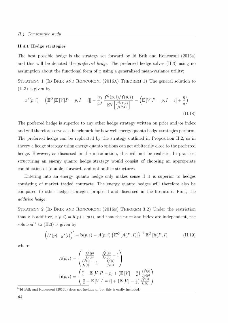
II.4. Comparative study
II.4.1 Hedge strategies
The best possible hedge is the strategy set forward by Id Brik and Roncoroni (2016a)
and this will be denoted the preferred hedge. The preferred hedge solves (II.3) using no
assumption about the functional form of x using a generalized mean-variance utility:
Strategy 1 (Id Brik and Roncoroni (2016a) Theorem 1) The general solution to
(II.3) is given by
x∗(p, i) =(EQ [E [V |P = p, I = i]]− η
a
) fQ(p, i)/f(p, i)
EQ[fQ(P ,I)f(P ,I)
] − (E [V |P = p, I = i] +η
a
)(II.18)
The preferred hedge is superior to any other hedge strategy written on price and/or index
and will therefore serve as a benchmark for how well energy quanto hedge strategies perform.
The preferred hedge can be replicated by the strategy outlined in Proposition II.2, so in
theory a hedge strategy using energy quanto options can get arbitrarily close to the preferred
hedge. However, as discussed in the introduction, this will not be realistic. In practice,
structuring an energy quanto hedge strategy would consist of choosing an appropriate
combination of (double) forward- and option-like structures.
Entering into an energy quanto hedge only makes sense if it is superior to hedges
consisting of market traded contracts. The energy quanto hedges will therefore also be
compared to other hedge strategies proposed and discussed in the literature. First, the
additive hedge:
Strategy 2 (Id Brik and Roncoroni (2016b) Theorem 3.2) Under the restriction
that x is additive, x(p, i) = h(p) + g(i), and that the price and index are independent, the
solution14 to (II.3) is given by(h∗(p) g∗(i)
)′= b(p, i)− A(p, i)
EQ [A(P , I)]
−1 EQ [b(P , I)] (II.19)
where
A(p, i) =
fQP (p)
fP (p)
fQP (p)
fP (p)− 1
fQI (i)
fI(i)− 1
fQI (i)
fI(i)
b(p, i) =
ηa− E [V |P = p] +
(E [V ]− η
a
) fQP (p)
fP (p)
ηa− E [V |I = i] +
(E [V ]− η
a
) fQI (i)
fI(i)
14Id Brik and Roncoroni (2016b) does not include η, but this is easily included.
64
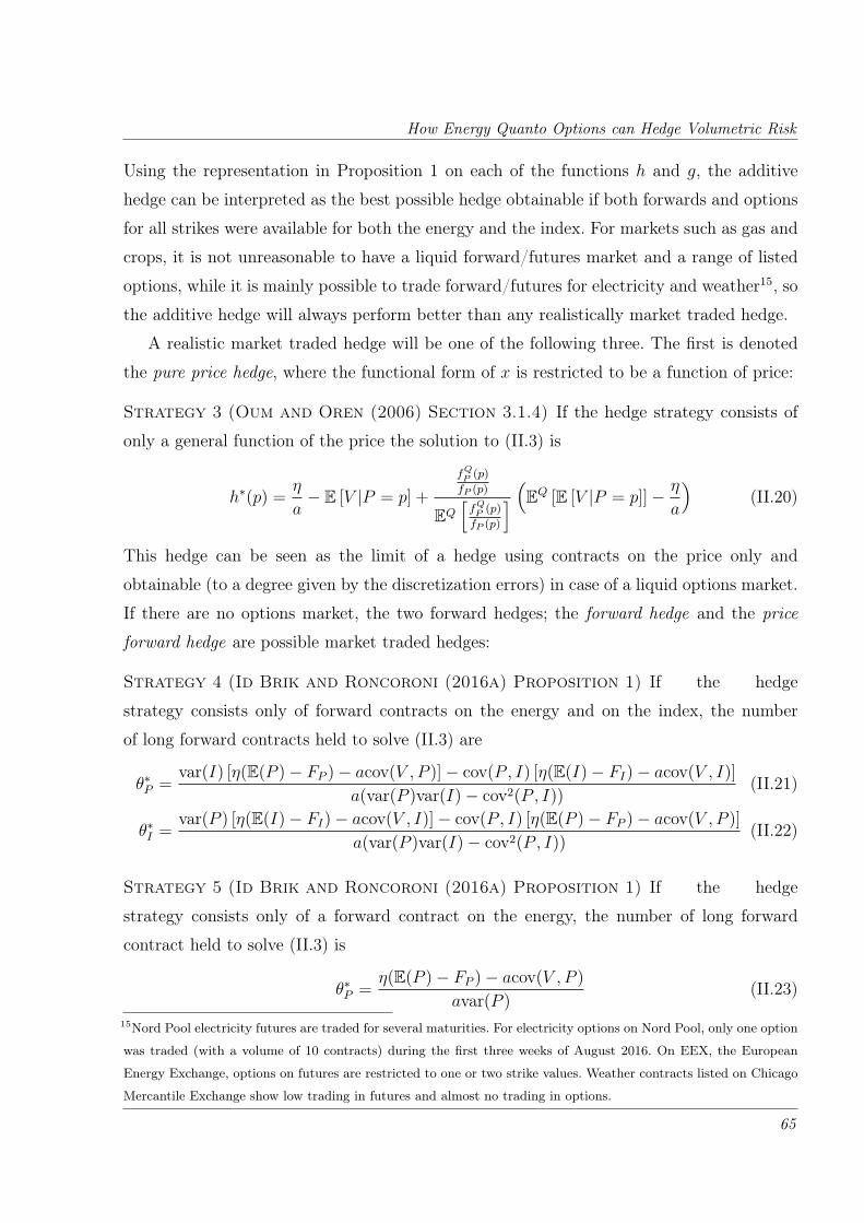
How Energy Quanto Options can Hedge Volumetric Risk
Using the representation in Proposition 1 on each of the functions h and g, the additive
hedge can be interpreted as the best possible hedge obtainable if both forwards and options
for all strikes were available for both the energy and the index. For markets such as gas and
crops, it is not unreasonable to have a liquid forward/futures market and a range of listed
options, while it is mainly possible to trade forward/futures for electricity and weather15, so
the additive hedge will always perform better than any realistically market traded hedge.
A realistic market traded hedge will be one of the following three. The first is denoted
the pure price hedge, where the functional form of x is restricted to be a function of price:
Strategy 3 (Oum and Oren (2006) Section 3.1.4) If the hedge strategy consists of
only a general function of the price the solution to (II.3) is
h∗(p) =η
a− E [V |P = p] +
fQP (p)
fP (p)
EQ[fQP (p)
fP (p)
] (EQ [E [V |P = p]]− η
a
)(II.20)
This hedge can be seen as the limit of a hedge using contracts on the price only and
obtainable (to a degree given by the discretization errors) in case of a liquid options market.
If there are no options market, the two forward hedges; the forward hedge and the price
forward hedge are possible market traded hedges:
Strategy 4 (Id Brik and Roncoroni (2016a) Proposition 1) If the hedge
strategy consists only of forward contracts on the energy and on the index, the number
of long forward contracts held to solve (II.3) are
θ∗P =var(I) [η(E(P )− FP )− acov(V ,P )]− cov(P , I) [η(E(I)− FI)− acov(V , I)]
a(var(P )var(I)− cov2(P , I))(II.21)
θ∗I =var(P ) [η(E(I)− FI)− acov(V , I)]− cov(P , I) [η(E(P )− FP )− acov(V ,P )]
a(var(P )var(I)− cov2(P , I))(II.22)
Strategy 5 (Id Brik and Roncoroni (2016a) Proposition 1) If the hedge
strategy consists only of a forward contract on the energy, the number of long forward
contract held to solve (II.3) is
θ∗P =η(E(P )− FP )− acov(V ,P )
avar(P )(II.23)
15Nord Pool electricity futures are traded for several maturities. For electricity options on Nord Pool, only one option
was traded (with a volume of 10 contracts) during the first three weeks of August 2016. On EEX, the European
Energy Exchange, options on futures are restricted to one or two strike values. Weather contracts listed on Chicago
Mercantile Exchange show low trading in futures and almost no trading in options.
65

II.4. Comparative study
These five strategies together with no hedge (the naked hedge) are compared to two
different quanto strategies. As previously mentioned, the structuring of energy quanto
hedge strategies requires different decisions regarding contract type, swap rates/strikes
and contract size. Using various combinations of contract structures from Proposition
II.2, different contract choices are analysed after inspecting the preferred hedge. Given the
contract structure, the choice of strikes and swap rates as well at the optimal number of each
contract are found using numerical optimization. The analysis is restricted to two simple
strategies, where the first uses a call-call energy quanto options (II.16) and the second uses
a call-call together with a put-put energy quanto option:
Strategy 6 (Simple quanto hedge) The hedge consists of forwards on the asset and the
index and one energy quanto call-call option with strikes KP and KI . The price of the
quanto option is denoted pQ:
x(p, i) = θP (p− FP ) + θI(i− FI) + θQ[(p−KP )+(i−KI)
+ − pQ]
(II.24)
Strategy 7 (Diagonal quanto hedge) The hedge consists of forwards on the asset and the
index, an energy quanto call-call option and an energy quanto put-put option with strikes
KP and KI . The prices of the quanto options are denoted pCCQ and pPPQ :
x(p, i) = θP (p− FP ) + θI(i− FI)+
+ θCCQ[(p−KP )+(i−KI)
+ − pCCQ]
+ θPPQ[(KP − p)+(KI − i)+ − pPPQ
](II.25)
II.4.2 Market design
The stylized gas market analysed by Id Brik and Roncoroni (2016a) is applied in this
comparative study and is described in Table II.1. All of the above strategies are easily
implementable for normally distributed and log-normally distributed variables. In Id Brik
and Roncoroni (2016a), price, quantity and index are all log-normally distributed16. In
e.g, Oum and Oren (2006) the analysis is also done under the assumption of quantity
being normally distributed. The comparative study is done for both set of distributional
assumptions. Parameters in (II.26) and (II.27) are chosen such that the mean and standard
deviations corresponds to those of Table II.1.16Although temperature can be negative, the index can for instance be thought of as the HDD index, which is by
definition always non-negative, so the assumption of log-normality is not inconsistent with representing temperature.
66
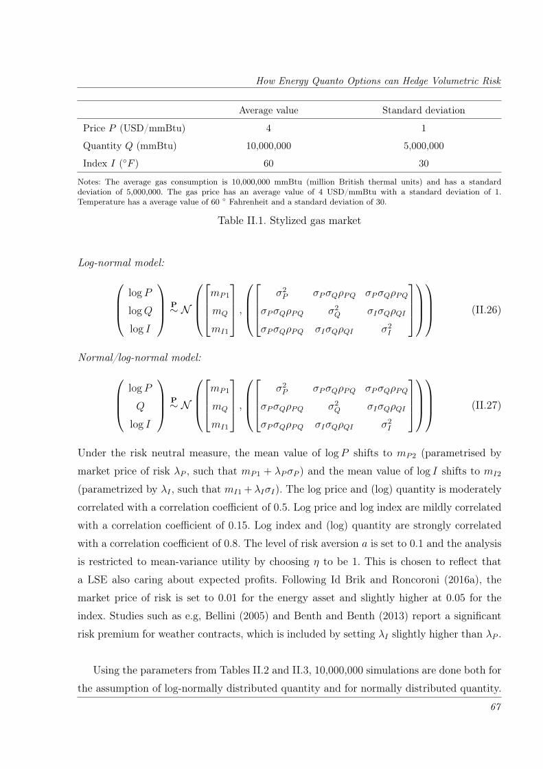
How Energy Quanto Options can Hedge Volumetric Risk
Average value Standard deviation
Price P (USD/mmBtu) 4 1
Quantity Q (mmBtu) 10,000,000 5,000,000
Index I (F ) 60 30
Notes: The average gas consumption is 10,000,000 mmBtu (million British thermal units) and has a standarddeviation of 5,000,000. The gas price has an average value of 4 USD/mmBtu with a standard deviation of 1.Temperature has a average value of 60 Fahrenheit and a standard deviation of 30.
Table II.1. Stylized gas market
Log-normal model:logP
logQ
log I
P∼ N
mP1
mQ
mI1
,
σ2P σPσQρPQ σPσQρPQ
σPσQρPQ σ2Q σIσQρQI
σPσQρPQ σIσQρQI σ2I
(II.26)
Normal/log-normal model:logP
Q
log I
P∼ N
mP1
mQ
mI1
,
σ2P σPσQρPQ σPσQρPQ
σPσQρPQ σ2Q σIσQρQI
σPσQρPQ σIσQρQI σ2I
(II.27)
Under the risk neutral measure, the mean value of logP shifts to mP2 (parametrised by
market price of risk λP , such that mP1 + λPσP ) and the mean value of log I shifts to mI2
(parametrized by λI , such that mI1 + λIσI). The log price and (log) quantity is moderately
correlated with a correlation coefficient of 0.5. Log price and log index are mildly correlated
with a correlation coefficient of 0.15. Log index and (log) quantity are strongly correlated
with a correlation coefficient of 0.8. The level of risk aversion a is set to 0.1 and the analysis
is restricted to mean-variance utility by choosing η to be 1. This is chosen to reflect that
a LSE also caring about expected profits. Following Id Brik and Roncoroni (2016a), the
market price of risk is set to 0.01 for the energy asset and slightly higher at 0.05 for the
index. Studies such as e.g, Bellini (2005) and Benth and Benth (2013) report a significant
risk premium for weather contracts, which is included by setting λI slightly higher than λP .
Using the parameters from Tables II.2 and II.3, 10,000,000 simulations are done both for
the assumption of log-normally distributed quantity and for normally distributed quantity.
67
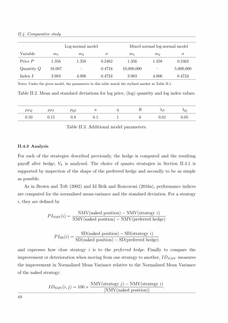
II.4. Comparative study
Log-normal model Mixed normal log-normal model
Variable m1 m2 σ m1 m2 σ
Price P 1.356 1.358 0.2462 1.356 1.358 0.2462
Quantity Q 16.007 – 0.4724 10,000,000 – 5,000,000
Index I 3.983 4.006 0.4724 3.983 4.006 0.4724
Notes: Under the given model, the parameters in this table match the stylized market in Table II.1.
Table II.2. Mean and standard deviations for log price, (log) quantity and log index values.
ρPQ ρPI ρQI a η R λP λQ
0.50 0.15 0.8 0.1 1 6 0.01 0.05
Table II.3. Additional model parameters.
II.4.3 Analysis
For each of the strategies described previously, the hedge is computed and the resulting
payoff after hedge, Vh is analysed. The choice of quanto strategies in Section II.4.1 is
supported by inspection of the shape of the preferred hedge and secondly to be as simple
as possible.
As in Brown and Toft (2002) and Id Brik and Roncoroni (2016a), performance indices
are computed for the normalised mean-variance and the standard deviation. For a strategy
i, they are defined by
PINMV(i) =NMV(naked position)− NMV(strategy i)
NMV(naked position)− NMV(preferred hedge)
PISD(i) =SD(naked position)− SD(strategy i)
SD(naked position)− SD(preferred hedge)
and expresses how close strategy i is to the preferred hedge. Finally to compare the
improvement or deterioration when moving from one strategy to another, IDNMV measures
the improvement in Normalized Mean Variance relative to the Normalized Mean Variance
of the naked strategy:
IDNMV(i, j) = 100× NMV(strategy j )− NMV(strategy i)|NMV(naked position)|
.
68

How Energy Quanto Options can Hedge Volumetric Risk
II.4.4 Results under assumption of log-normally distributed quantity
The surface plots in Figure II.1 shows the preferred hedge and the forward hedge as a
function of price p and index i and illustrates what the LSE is concerned about: Looking
at the dimensions one by one, it is seen that the higher the price, the more payoff the LSE
would like from their hedge. This is also obtained in the forward hedge. But for the index,
the LSE would like less for higher values of the index if the price is low, while they would
like more for higher values of the index if the price is high. With the forward hedge, they
can only obtain the same slope regardless of price. For this example, it results in shorting
forwards on the index.
A payoff in the high price-high index situation is exactly obtained by buying a call-call
quanto option together with a number of forwards. This was denoted to as the simple quanto
hedge. Looking more closely at the preferred hedge’s surface in II.1, there is also a slight
increase in the function value for low price and low index. It might therefore add extra value
to add a put-put quanto option to the simple quanto strategy. This was referred to as the
diagonal quanto hedge.
In Figure II.3 selected profit distributions are compared: The left panel shows the
preferred hedge together with the naked strategy as well as the simple quanto hedge. The
right panel shows the preferred hedge, the simple quanto hedge and the additive hedge. The
simple quanto hedge seems to do better than the additive hedge and as this will outperform
all other described strategies, the simple quanto hedge is a strong candidate for a hedge
strategy with a feasible design.
Table II.4 shows performance statistics for the hedge strategies described in section II.4.1.
The columns present the expected utility for a mean-variance hedge, the expected profit, the
standard deviation, the normalised mean-variance (defined as the expected profit net of the
standard deviation), the probability of a loss, the 5% Value-at-Risk and the 5% Expected
Shortfall17. Regardless of performance measure, when quantity is log-normally distributed,
the simple quanto hedge and the diagonal quanto hedge is doing almost equally well.
Table II.5 shows the performance both for the normalised mean-variance and for a pure
variance measure of performance. The discrepancy between any of the two quanto hedges and
17For VaR and ES, a negative number indicates a gain. The average margin is 2$ and a loss is therefore not very likely
in this setup. The unrealistically large margin is kept to allow for a direct comparison with Id Brik and Roncoroni
(2016a).
69
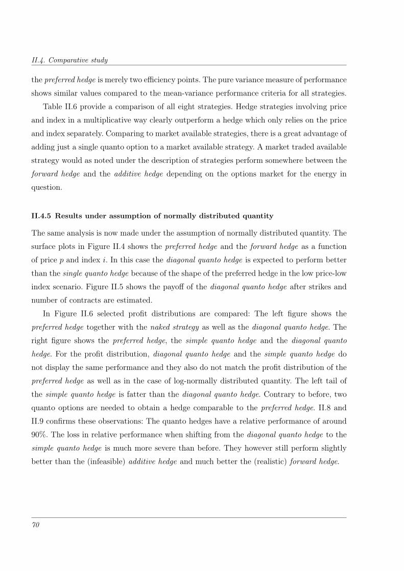
II.4. Comparative study
the preferred hedge is merely two efficiency points. The pure variance measure of performance
shows similar values compared to the mean-variance performance criteria for all strategies.
Table II.6 provide a comparison of all eight strategies. Hedge strategies involving price
and index in a multiplicative way clearly outperform a hedge which only relies on the price
and index separately. Comparing to market available strategies, there is a great advantage of
adding just a single quanto option to a market available strategy. A market traded available
strategy would as noted under the description of strategies perform somewhere between the
forward hedge and the additive hedge depending on the options market for the energy in
question.
II.4.5 Results under assumption of normally distributed quantity
The same analysis is now made under the assumption of normally distributed quantity. The
surface plots in Figure II.4 shows the preferred hedge and the forward hedge as a function
of price p and index i. In this case the diagonal quanto hedge is expected to perform better
than the single quanto hedge because of the shape of the preferred hedge in the low price-low
index scenario. Figure II.5 shows the payoff of the diagonal quanto hedge after strikes and
number of contracts are estimated.
In Figure II.6 selected profit distributions are compared: The left figure shows the
preferred hedge together with the naked strategy as well as the diagonal quanto hedge. The
right figure shows the preferred hedge, the simple quanto hedge and the diagonal quanto
hedge. For the profit distribution, diagonal quanto hedge and the simple quanto hedge do
not display the same performance and they also do not match the profit distribution of the
preferred hedge as well as in the case of log-normally distributed quantity. The left tail of
the simple quanto hedge is fatter than the diagonal quanto hedge. Contrary to before, two
quanto options are needed to obtain a hedge comparable to the preferred hedge. II.8 and
II.9 confirms these observations: The quanto hedges have a relative performance of around
90%. The loss in relative performance when shifting from the diagonal quanto hedge to the
simple quanto hedge is much more severe than before. They however still perform slightly
better than the (infeasible) additive hedge and much better the (realistic) forward hedge.
70
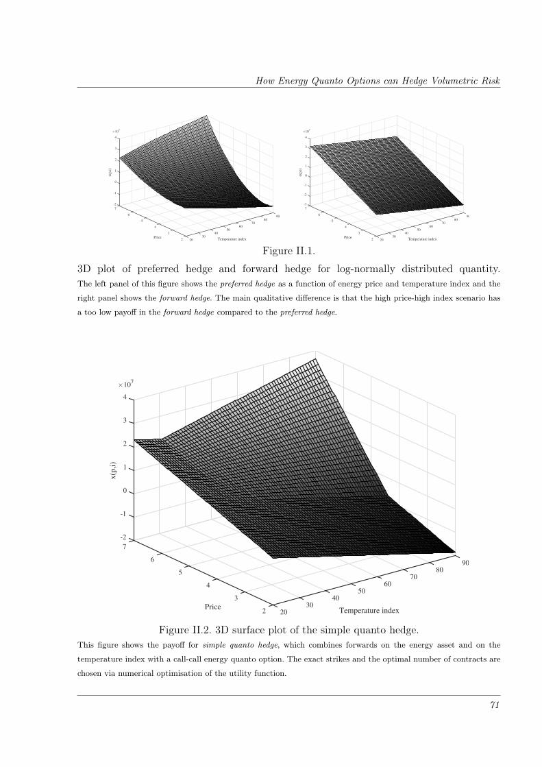
How Energy Quanto Options can Hedge Volumetric Risk
9080
70
Temperature index
6050
4030
202
3
Price
4
5
6
×107
3
-2
-1
0
4
1
2
7
x(p
,i)
9080
70
Temperature index
6050
4030
202
3
Price
4
5
6
×107
4
-3
-2
-1
0
1
3
2
7
x(p
,i)
Figure II.1.
3D plot of preferred hedge and forward hedge for log-normally distributed quantity.The left panel of this figure shows the preferred hedge as a function of energy price and temperature index and the
right panel shows the forward hedge. The main qualitative difference is that the high price-high index scenario has
a too low payoff in the forward hedge compared to the preferred hedge.
9080
70
Temperature index
6050
4030
202
3
Price
4
5
6
×107
3
-2
-1
0
4
1
2
7
x(p
,i)
Figure II.2. 3D surface plot of the simple quanto hedge.This figure shows the payoff for simple quanto hedge, which combines forwards on the energy asset and on the
temperature index with a call-call energy quanto option. The exact strikes and the optimal number of contracts are
chosen via numerical optimisation of the utility function.
71
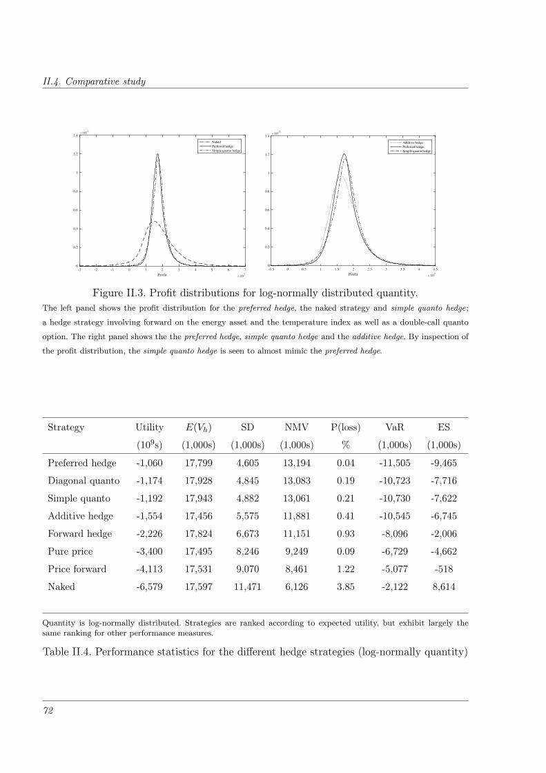
II.4. Comparative study
Profit×10
7
-3 -2 -1 0 1 2 3 4 5 6 7
×10-7
0
0.2
0.4
0.6
0.8
1
1.2
1.4
Naked
Preferred hedge
Simple quanto hedge
Profit×10
7
-0.5 0 0.5 1 1.5 2 2.5 3 3.5 4 4.5
×10-7
0
0.2
0.4
0.6
0.8
1
1.2
1.4
Additive hedge
Preferred hedge
Simple quanto hedge
Figure II.3. Profit distributions for log-normally distributed quantity.The left panel shows the profit distribution for the preferred hedge, the naked strategy and simple quanto hedge;
a hedge strategy involving forward on the energy asset and the temperature index as well as a double-call quanto
option. The right panel shows the the preferred hedge, simple quanto hedge and the additive hedge. By inspection of
the profit distribution, the simple quanto hedge is seen to almost mimic the preferred hedge.
Strategy Utility E(Vh) SD NMV P(loss) VaR ES
(109s) (1,000s) (1,000s) (1,000s) % (1,000s) (1,000s)
Preferred hedge -1,060 17,799 4,605 13,194 0.04 -11,505 -9,465
Diagonal quanto -1,174 17,928 4,845 13,083 0.19 -10,723 -7,716
Simple quanto -1,192 17,943 4,882 13,061 0.21 -10,730 -7,622
Additive hedge -1,554 17,456 5,575 11,881 0.41 -10,545 -6,745
Forward hedge -2,226 17,824 6,673 11,151 0.93 -8,096 -2,006
Pure price -3,400 17,495 8,246 9,249 0.09 -6,729 -4,662
Price forward -4,113 17,531 9,070 8,461 1.22 -5,077 -518
Naked -6,579 17,597 11,471 6,126 3.85 -2,122 8,614
Quantity is log-normally distributed. Strategies are ranked according to expected utility, but exhibit largely thesame ranking for other performance measures.
Table II.4. Performance statistics for the different hedge strategies (log-normally quantity)
72

How Energy Quanto Options can Hedge Volumetric Risk
Strategy Performance (NMV) Performance (SD)
Preferred hedge 1.00 1.00
Diagonal quanto 0.98 0.97
Simple quanto 0.98 0.96
Additive hedge 0.81 0.86
Forward hedge 0.71 0.70
Pure price 0.44 0.47
Price forward 0.33 0.35
Naked 0.00 0.00
Notes: The table dispays the performance of hedge strategies compared to the preferred hedge and the naked profits,when quantity is log-normally distributed. If the performance index is equal to 1, the strategy is doing as well as thepreferred hedge. The quanto strategies both have a 0.98 performance when measured in relation to the normalisedmean-variance and a performance of 0.96-0.97 in terms of decreasing the standard deviation of profits.
Table II.5. Performance of strategies
Preferred
hedge
Diagonal
quanto
Simple
quanto
Additive
hedge
Forward
hedge
Pure
price
Price
for-
ward
Naked
Preferred hedge 0.00 -1.82 -2.16 -21.42 -33.34 -64.39 -77.25 -115.36
Diagonal quanto 1.82 0.00 -0.35 -19.61 -31.52 -62.58 -75.44 -113.54
Simple quanto 2.16 0.35 0.00 -19.26 -31.18 -62.23 -75.09 -113.20
Additive hedge 21.42 19.61 19.26 0.00 -11.92 -42.97 -55.83 -93.93
Forward hedge 33.34 31.52 31.18 11.92 0.00 -31.05 -43.91 -82.02
Pure price 64.39 62.58 62.23 42.97 31.05 0.00 -12.86 -50.96
Price forward 77.25 75.44 75.09 55.83 43.91 12.86 0.00 -38.10
Naked 115.36 113.54 113.20 93.93 82.02 50.96 38.10 0.00
Notes: The tables show the relative improvement or deterioration, when going from one hedge to another in the caseof log-normally distributed quantity. The preferred hedge and the two quanto hedges are very close to each otherand there is almost no difference between the two quanto hedges.
Table II.6. Relative improvement or deterioration for hedge strategies
73

II.4. Comparative study
9080
70
Temperature index
6050
4030
202
3
Price
4
5
6
×107
3
-2
-1
0
4
1
2
7
x(p
,i)
9080
70
Temperature index
6050
4030
202
3
Price
4
5
6
×107
4
-3
-2
-1
0
1
3
2
7
x(p
,i)
Figure II.4. 3D plot of preferred hedge and forward hedge for normally distributed quantity.The left panel of this figure shows the preferred hedge as a function of energy price and temperature index and the
right panel shows the forward hedge. The main qualitative difference is that the high price-high index scenario and
the low price-low index scenario has a too low payoff in the forward hedge relative to the preferred hedge. Compared
to the log-normally distributed quantity, the LSE would like a much higher payoff in the low price-low index scenario.
9080
70
Temperature index
6050
4030
202
3
Price
4
5
6
×107
4
-3
-2
-1
0
1
3
2
7
x(p
,i)
Figure II.5. 3D surface plot of the diagonal quanto hedge.This figure shows the payoff for diagonal quanto hedge, which combines forwards on the energy asset and on the
temperature index with a call-call and a put-put energy quanto option. The exact strikes and the optimal number
of contracts are chosen via numerical optimisation of the utility function.
74
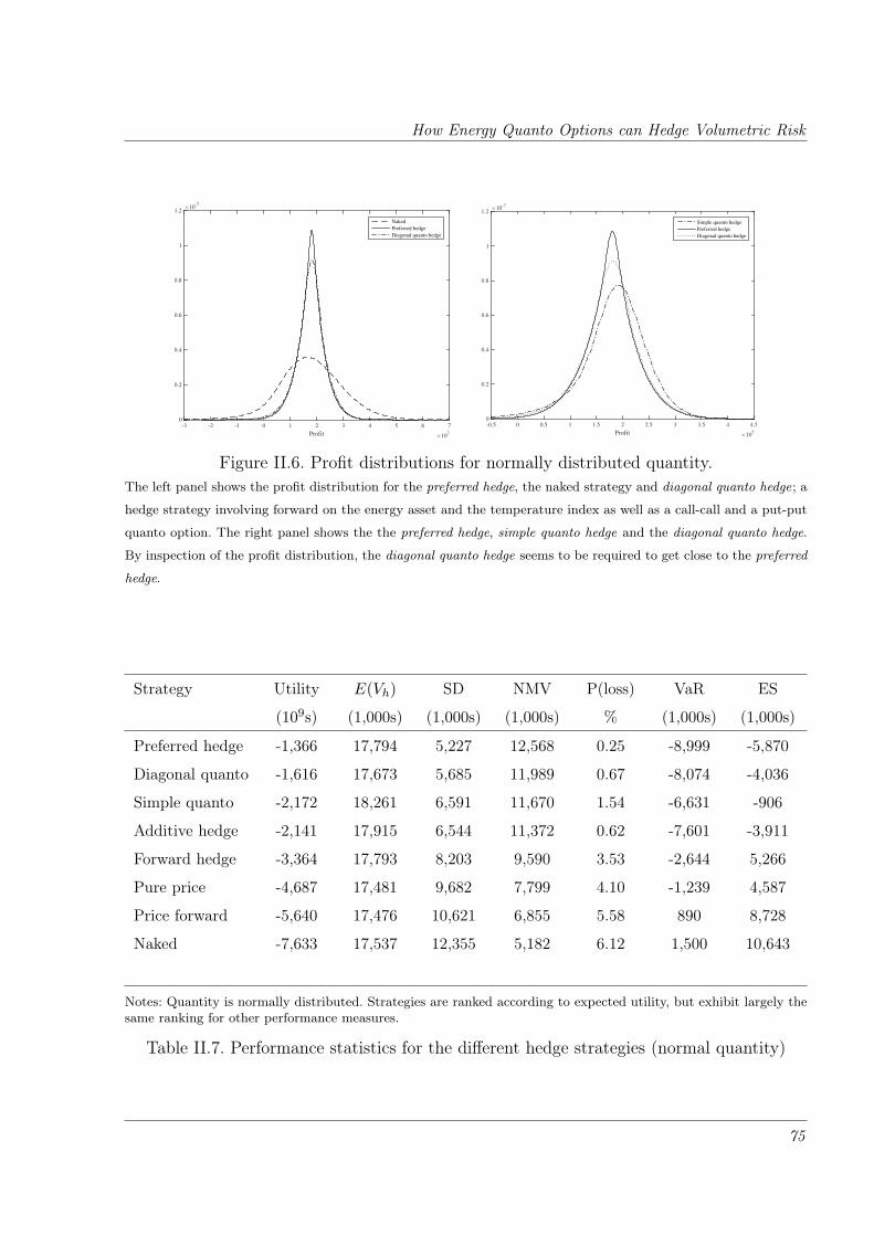
How Energy Quanto Options can Hedge Volumetric Risk
Profit×10
7
-3 -2 -1 0 1 2 3 4 5 6 7
×10-7
0
0.2
0.4
0.6
0.8
1
1.2
Naked
Preferred hedge
Diagonal quanto hedge
Profit×10
7
-0.5 0 0.5 1 1.5 2 2.5 3 3.5 4 4.5
×10-7
0
0.2
0.4
0.6
0.8
1
1.2
Simple quanto hedge
Preferred hedge
Diagonal quanto hedge
Figure II.6. Profit distributions for normally distributed quantity.The left panel shows the profit distribution for the preferred hedge, the naked strategy and diagonal quanto hedge; a
hedge strategy involving forward on the energy asset and the temperature index as well as a call-call and a put-put
quanto option. The right panel shows the the preferred hedge, simple quanto hedge and the diagonal quanto hedge.
By inspection of the profit distribution, the diagonal quanto hedge seems to be required to get close to the preferred
hedge.
Strategy Utility E(Vh) SD NMV P(loss) VaR ES
(109s) (1,000s) (1,000s) (1,000s) % (1,000s) (1,000s)
Preferred hedge -1,366 17,794 5,227 12,568 0.25 -8,999 -5,870
Diagonal quanto -1,616 17,673 5,685 11,989 0.67 -8,074 -4,036
Simple quanto -2,172 18,261 6,591 11,670 1.54 -6,631 -906
Additive hedge -2,141 17,915 6,544 11,372 0.62 -7,601 -3,911
Forward hedge -3,364 17,793 8,203 9,590 3.53 -2,644 5,266
Pure price -4,687 17,481 9,682 7,799 4.10 -1,239 4,587
Price forward -5,640 17,476 10,621 6,855 5.58 890 8,728
Naked -7,633 17,537 12,355 5,182 6.12 1,500 10,643
Notes: Quantity is normally distributed. Strategies are ranked according to expected utility, but exhibit largely thesame ranking for other performance measures.
Table II.7. Performance statistics for the different hedge strategies (normal quantity)
75
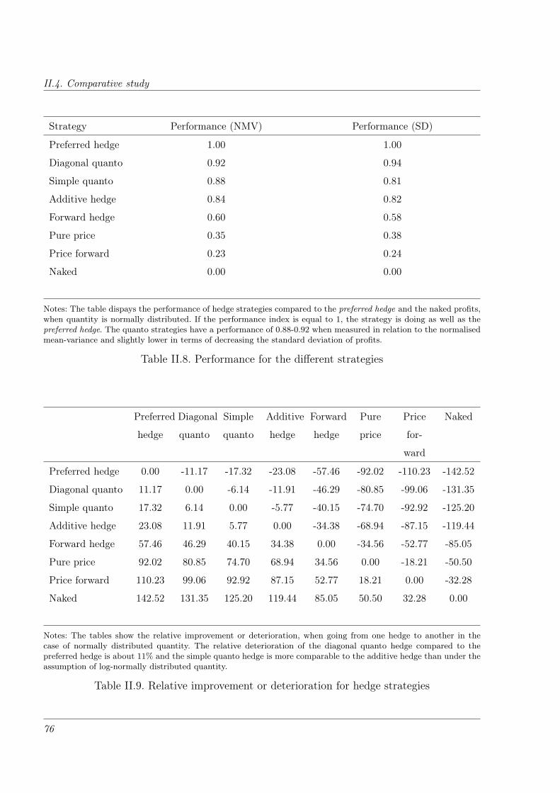
II.4. Comparative study
Strategy Performance (NMV) Performance (SD)
Preferred hedge 1.00 1.00
Diagonal quanto 0.92 0.94
Simple quanto 0.88 0.81
Additive hedge 0.84 0.82
Forward hedge 0.60 0.58
Pure price 0.35 0.38
Price forward 0.23 0.24
Naked 0.00 0.00
Notes: The table dispays the performance of hedge strategies compared to the preferred hedge and the naked profits,when quantity is normally distributed. If the performance index is equal to 1, the strategy is doing as well as thepreferred hedge. The quanto strategies have a performance of 0.88-0.92 when measured in relation to the normalisedmean-variance and slightly lower in terms of decreasing the standard deviation of profits.
Table II.8. Performance for the different strategies
Preferred
hedge
Diagonal
quanto
Simple
quanto
Additive
hedge
Forward
hedge
Pure
price
Price
for-
ward
Naked
Preferred hedge 0.00 -11.17 -17.32 -23.08 -57.46 -92.02 -110.23 -142.52
Diagonal quanto 11.17 0.00 -6.14 -11.91 -46.29 -80.85 -99.06 -131.35
Simple quanto 17.32 6.14 0.00 -5.77 -40.15 -74.70 -92.92 -125.20
Additive hedge 23.08 11.91 5.77 0.00 -34.38 -68.94 -87.15 -119.44
Forward hedge 57.46 46.29 40.15 34.38 0.00 -34.56 -52.77 -85.05
Pure price 92.02 80.85 74.70 68.94 34.56 0.00 -18.21 -50.50
Price forward 110.23 99.06 92.92 87.15 52.77 18.21 0.00 -32.28
Naked 142.52 131.35 125.20 119.44 85.05 50.50 32.28 0.00
Notes: The tables show the relative improvement or deterioration, when going from one hedge to another in thecase of normally distributed quantity. The relative deterioration of the diagonal quanto hedge compared to thepreferred hedge is about 11% and the simple quanto hedge is more comparable to the additive hedge than under theassumption of log-normally distributed quantity.
Table II.9. Relative improvement or deterioration for hedge strategies
76
How Energy Quanto Options can Hedge Volumetric Risk
II.5 Concluding remarks
The representation of a hedge strategy based on both price and an index correlated to
quantity contains energy quanto options and swaps. Using a standard one-period example,
it was shown that realistic strategies including one or two quanto options perform almost
as well as the unrealistic ideal hedge strategy.
The randomness in price, quantity and index was modelled using a multivariate normal
distribution. The quantity had in both analyses the same mean and variance, but followed
either a log-normal or a normal distribution. The difference impacted the shape of the ideal
hedge and thereby also which quanto strategy was needed. It is reasonable to assume that
there is no universal energy quanto structure, when it comes to hedging volumetric and
price risk jointly. Rather, the exact choice must be based on studies of the marginal and
joint distribution of price, quantity and index for the exact market in question.
As discussed in Section II.2, a one period model is not realistic for many energy
applications. In a multi-period framework, simulation studies must be conducted including
necessary analyses of correlation structures across variables as well as choosing an
appropriate pricing approach. If the counterpart is a re-insurance company, pricing under
the physical measure and adding a premium to ensure an acceptable risk level could be
reasonable. It is reasonable to assume that strategies involving energy quanto contracts
can improve risk management also in the multi-period setting, as it offers a multiplicative
contract structure to take care of the embedded multiplicative risk.
The results of this simple analysis provide an argument for why a Load Serving Entity
should also consider OTC options rather than only market traded instruments, when they
are designing their hedge.
77
II.A. Details of benchmark strategies
Appendix
II.A Details of benchmark strategies
II.A.1 Preferred hedge
The preferred hedge using a mean-variance approach is a function of price value p and index
value i. It is denoted x∗ and is given as
x∗(p, i) =(EQ [E [V |P = p, I = i]]− η
a
) fQ(p, i)/f(p, i)
EQ[fQPI(P ,I)
fPI(P ,I)
] − (E [V |P = p, I = i] +η
a
).
(II.28)
The above expression is derived under that assumption that both price, quantity and index
are log-normally distributed:logP
logQ
log I
P∼ N
mP1
mQ
mI1
,
σ2P σPσQρPQ σPσQρPQ
σPσQρPQ σ2Q σIσQρQI
σPσQρPQ σIσQρQI σ2I
. (II.29)
Under the risk neutral measure, the mean value shifts to[mP2 mQ mI2
]′. In the end of
this subsection, (II.28) is also derived for normally distributed quantity and index. In the
following the notation from Id Brik and Roncoroni (2016a) is adopted:
u =
(log p
log i
), U =
(logP
log I
), mu1 = EP (U), mu2 = EQ(U),
Σ = Var(U), b =
(σPσQρPQ
σIσQρQI
)The individual terms of (II.28) are now considered. First the density ratio of the marginal
distributions:fQPI(p, i)
fPI(p, i)= exp
12
(u−mu1)′Σ−1 (u−mu1)− 12
(u−mu2)′Σ−1 (u−mu2)
= exp
(mu2 −mu1)′Σ−1u− 12
(mu2 −mu1)′Σ−1 (mu1 +mu2)
(II.30)
78
How Energy Quanto Options can Hedge Volumetric Risk
The expected value of this under Q is then assessed. Everything inside the exp is normally
distributed with mean value (mu2 −mu1)′Σ−1mu2 − 12
(mu2 −mu2)′Σ−1 (mu1 +mu2) and
variance (mu2 −mu1)′Σ−1 (mu2 −mu1) This results in
EQ[fQPI(P , I)
fPI(P , I)
]= exp
(mu2 −mu1)′Σ−1 (mu2 −mu1)
(II.31)
Next, the expected profit equals
E [V |P = p, I = i] = (R− p)E [Q|P = p, I = i] = (R− p)E[elogQ|P = p, I = i
]As logQ given P = p and I = i is conditionally normal with mean and variance
mQ + b′Σ−1(u−mu1)
σ2Q − b′Σ−1b
the conditional expected value of the unhedged profit is given as
E [V |P = p, I = i] = (R− p) expmQ + 1
2σ2Q + b′Σ−1(u−mu1 − b/2)
. (II.32)
The expectation under Q value of this is
EQ [E [V |P , I]] = EQ[(R− P ) exp
mQ + 1
2σ2Q + b′Σ−1(U−mu1 − b/2)
]= R exp
mQ + 1
2σ2Q
EQ[exp
b′Σ−1(U−mu1 − b/2)
]− exp
mQ + 1
2σ2Q
EQ[exp
[1 0
]U + b′Σ−1(U−mu1 − b/2)
]= exp
mQ + 1
2σ2Q + b′Σ−1(mu2 −mu1)
×(R− exp
mP2 + 1
2σ2P + σPσQρPQ
)(II.33)
Note that (II.30) and (II.31) would also hold if the price and/or index was normally
distributed instead of assumption (II.29). It would only require a change of the definition
of u. The two other expressions (II.32) and (II.33) are also available in closed form for any
of the eight normal/log-normal combination of (II.29). The derivation is restricted to the
case where price is log-normally distributed and the quantity is normally distributed. The
index may follow either distribution. When Q is normally distributed, then
E [V |P = p, I = i] = (R− p)(mQ + b′Σ−1(u−mu1)
)(II.34)
79
II.A. Details of benchmark strategies
with u defined appropriately. The expectation under Q is:
EQ [E [V |P , I]] = EQ[(R− P )
(mQ + b′Σ−1(U−mu1)
)]= R
(mQ + b′Σ−1(mu2 −mu1)
)−mQe
mP2+σ2P
2
− b′Σ−1EQ[PU1
PU2
]+ b′Σ−1mu1e
mP2+σ2P
2
For log-normally distributed price (i.e., U1 = logP ), then
EQ [P logP ] = emP2+σ2P
2(σ2P +mP2
)and
EQ [PU2] = emP2+σ2P
2 (σPσIρPI +mI2) ,
resulting in
EQ [E [V |P , I]] =
(R− emP2+
σ2P
2
)(mQ + b′Σ−1(mu2 −mu1)
)− emP2+
σ2P
2 b′Σ−1
[σ2P
σPσIρPI
](II.35)
II.A.2 Additive hedge
The additive hedge using a mean-variance approach consists of two functions, one of price
value p and one on index value i. They are denoted h∗(p) and g∗(i) and are given as(h∗(p) g∗(i)
)′= b(p, i)− A(p, i)
EQ [A(P , I)]
−1 EQ [b(P , I)] (II.36)
where
A(p, i) =
fQP (p)
fP (p)
fQP (p)
fP (p)− 1
fQI (i)
fI(i)− 1
fQI (i)
fI(i)
b(p, i) =
1a− E [V |P = p] +
(E [V ]− 1
a
) fQP (p)
fP (p)
1a− E [V |I = i] +
(E [V ]− 1
a
) fQI (i)
fI(i)
The above expression is derived under that assumption that price, quantity and index are
log-normally distributed (again, the assumption regarding quantity is later replaced by a
normal distribution). Further, it is assumed that price and index is uncorrelated:logP
logQ
log I
P∼ N
mP1
mQ
mI1
,
σ2P σPσQρPQ 0
σPσQρPQ σ2Q σIσQρQI
0 σIσQρQI σ2I
.
80
How Energy Quanto Options can Hedge Volumetric Risk
As before; under the risk neutral measure, the mean value shifts to[mP2 mQ mI2
]′. The
individual expressions of (II.36) are now considered. First the ratio of the marginal densities:
fQP (p)
fP (p)= exp
1
2σ2P
(log p−mP1)2 − 12σ2P
(log p−mP2)2
= exp
1σ2P
(mP2 −mP1) log p− 12σ2P
(mP2 −mP1) (mP1 +mP2)
(II.37)
The expected value of this under Q is then calculated. Everything inside the exp is
normally distributed with mean value 1σ2P
(mP2 −mP1)mP2− 12σ2P
(mP2 −mP1) (mP1 +mP2)
and variance 1σ2P
(mP2 −mP1)2 This results in
EQ[fQP (P )
fP (P )
]= exp
1σ2P
(mP2 −mP1)2
. (II.38)
The same expressions holds for the index. Next, the expected profit expressions:
E [V |P = p] = (R− p)E [Q|P = p] = (R− p)E[elogQ|P = p
]As logQ given P = p is conditionally normal with mean and variance
mQ + ρPQσQσP
(log p−mP1) and σ2Q(1− ρ2
PQ)
the conditional expected value of the unhedged profit is given as
E [V |P = p] = (R− p) exp
mQ + ρPQ
σQσP
(log p−mP1) + 12σ2Q(1− ρ2
PQ)
. (II.39)
The expectation under Q value of this is
EQ [E [V |P ]] = EQ[(R− P ) exp
mQ + ρPQ
σQσP
(log p−mP1) + 12σ2Q(1− ρ2
PQ)
]= R exp
mQ + 1
2σ2Q(1− ρ2
PQ)EQ[exp
ρPQ
σQσP
(log p−mP1)
]− exp
mQ + 1
2σ2Q(1− ρ2
PQ)− ρPQσQσPmP1
EQ[exp
(1 + ρPQ
σQσP
)log p
]= exp
mQ + 1
2σ2Q + ρPQ
σQσP
(m −mP1)
(R− exp
mp2 + 1
2σ2P + ρPQσQσP
)(II.40)
Expected unhedged profits given I = i:
E [V |I = i] = E [(R− P )Q|I = i] = RE[elogQ|I = i
]− E
[elogP+logQ|I = i
]81
II.A. Details of benchmark strategies
As (logP , logQ) given I = i is bivariate normal with mean and variance(mP1
mQ + ρQIσQσI
(log i−mI1)
)and
(σ2P ρPQσPσQ
ρPQσPσQ σ2Q(1− ρ2
QI)
),
the expected value of the unhedged profit conditional on I = i is given as
E [V |I = i] =(R− exp
mP1 + 1
2σ2P + ρPQσPσQ
)×
exp
mQ + ρQI
σQσI
(log i−mI1) + 12σ2Q(1− ρ2
QI)
. (II.41)
Taking Q expectations of this yields
EQ [E [V |I]] =(R− exp
mP1 + 1
2σ2P + ρPQσPσQ
)exp
mQ + ρQI
σQσI
(mI2 −mI1) + 12σ2Q
.
(II.42)
The unconditional P-expectation of the unhedged profit becomes
E [V ] = E [E [V |I]] =(R− exp
mP1 + 1
2σ2P + ρPQσPσQ
)exp
mQ + 1
2σ2Q
. (II.43)
If Q instead of logQ given P = p is conditionally normal, then the conditional expected
value of the unhedged profit is given as
E [V |P = p] = (R− p)mQ + ρPQ
σQσP
(log p−mP1)
(II.44)
and the expectation under Q is
EQ [E [V |P ]] =
(R− emP2+
σ2P
2
)mQ + ρPQ
σQσP
(mp2 −mP1)
− emP2+
σ2P
2 ρPQσQσP .
(II.45)
The expected unhedged profit given I = i becomes:
E [V |I = i] = E [(R− P )Q|I = i] = RE [Q|I = i]− E[QelogP |I = i
].
As (logP ,Q) given I = i is bivariate normal with mean and variance(mP1
mQ + ρQIσQσI
(log i−mI1)
)and
(σ2P ρPQσPσQ
ρPQσPσQ σ2Q(1− ρ2
QI)
),
the conditional on i expected value of the unhedged profit is given as
E [V |I = i] = (R− emP1+12σ2P )
(mQ + ρQI
σQσI
(log i−mI1)
)− emP1+
12σ2PσPσQρPQ (II.46)
82

How Energy Quanto Options can Hedge Volumetric Risk
Taking Q expectations of this yields
EQ [E [V |I]] = (R− emP1+12σ2P )
(mQ + ρQI
σQσI
(mI2 −mI1)
)− emP1+
12σ2PσPσQρPQ (II.47)
with the unconditional P-expectation of the unhedged profit:
E [V ] = E [E [V |I]] = (R− emP1+12σ2P )mQ − emP1+
12σ2PσPσQρPQ (II.48)
83

Pricing and Hedging Energy Quanto Options
Essay III
Pricing and Hedging Energy Quanto Options∗
Co-authored with Fred Espen Benth, University of Oslo and Tor Åge Myklebust, Cancer
Registry of Norway. Published in the Journal of Energy Markets (2015), 8(1), p. 1–35. Due
to journal guidelines, Appendix III.E was incorporated in the main text in the published
version of this paper. I have chosen to keep this analysis in the appendix in this version.
Abstract
In energy markets, the use of quanto options has increased significantly in recent
years. The payoff from such options are typically written on an underlying energy
index and a measure of temperature. They are suited to managing the joint price
and volume risk in energy markets. Using a Heath-Jarrow-Morton approach, we
derive a closed-form option pricing formula for energy quanto options under the
assumption that the underlying assets are lognormally distributed. Our approach
encompasses several interesting cases, such as geometric Brownian motions and
multifactor spot models. We also derive Delta and Gamma expressions for hedging.
Further, we illustrate the use of our model by an empirical pricing exercise using
New York Mercantile Exchange-traded natural gas futures and Chicago Mercantile
Exchange-traded heating degree days futures for New York.
∗We thank participants from the Wolfgang Pauli Institute’s Conference on Energy Finance 2012 in Vienna, the
Energy Finance Conference 2012 in Trondheim, the 4th International Ruhr Energy Conference (INREC) 2013 in
Essen and the Energy Finance Christmas Workshop 2013 in Oslo for helpful feedback and suggestions. Editorial
processing of the published version of this paper was undertaken by Ruediger Kiesel. Fred Espen Benth thanks the
Norwegian Research Council for financial support.
85
III.1. Introduction
III.1 Introduction
Many industries are exposed to the variability of the weather. Take, as an example, a
gas distribution company that operates in an open wholesale market. Their planned sales
volumes per day and the market price are the two main factors to which they are exposed.
If, for example, one of the winter months turns out to be warmer than usual, the demand
for gas would drop. This decline in demand would probably also affect the market price
for gas, leading to a drop in gas price. The firm would make a loss compared with their
planned revenue, which is equal to the shortfall in demand multiplied by the difference
between the retail price at which they would have sold had their customers bought the
gas, and the market price at which they must now sell their excess gas. So, they face not
only a direct weather effect, eg, the lower demand, but also an indirect effect through the
drop in market prices. The above example clearly illustrates that the adverse movements
in market price and demand due to higher temperatures represent a kind of correlation
risk, which is difficult to properly hedge against, as it leads to a heavier tailed profit-and-
loss distribution. Using standard weather derivatives as offered by the Chicago Mercantile
Exchange (CME) would most likely represent an imperfect and rather expensive hedging
strategy, as it accounts only for the direct earnings effect from the change in demand, and
not the indirect earnings effect from price changes. If standardized weather products are
insufficient as hedging tools, the companies must turn to over-the-counter (OTC) markets
for weather derivatives. Davis (2010) and Pérez-González and Yun (2013) refer to surveys
conducted by the Weather Risk Management Association (WRMA) and reports from the
CME about market sizes and expected development:1 the market for standardized weather
derivatives peaked in 2007 with a total volume of trades close to 930,000 and a corresponding
notional value of US$17.9 billion. Since 2008, the market for standardized contracts has
experienced severe retrenchment. In 2009, the total volume of trades dipped below 500,000,
amounting to a notional value of around US$5.3 billion. A big part of this sharp decline is
attributed to the substantial increase, eg, 30% from 2010 to 2011, in the market for tailor-
made contracts, especially the quantity-adjusting weather contracts (”quanto”). Contracts
of this type worth US$100 million have been reported. Market participants indicate that
1Although the reported numbers are small compared with other markets, weather-exposed utilities can use weather
derivatives to reduce extreme losses from weather incidents and increase the valuation of the company (see Pérez-
González and Yun (2013) for an extensive study of the effect of weather derivatives on firm value, investments and
leverage).
86

Pricing and Hedging Energy Quanto Options
the demand for quanto contracts is international, with transactions being executed in the
United States, Europe, Australia and South America. In 2010, the WRMA believed that
the developing market in India alone had a potential value of US$2.35 billion.
The label ”quanto options” has traditionally been assigned to a class of derivatives
in financial markets where the investor wishes to be exposed to price movements in the
foreign asset without the corresponding exchange rate risk. The pricing of currency quanto
options has been extensively researched and dates back to the original work of Garman and
Kohlhagen (1983). Although the same term is used for the specific type of energy options
that we study in this paper, these two types of derivatives contracts are different: a typical
currency quanto option has a regular call-put payoff structure, whereas the energy quanto
options we study have a payoff structure similar to a product of call-put options, and energy
quanto options are therefore mainly used to hedge exposure to the joint price and volume
risk.2 In comparison with studies of currency quantos, research related to the pricing of
quanto options in energy markets is scarce. One exception is Caporin et al. (2012), who
propose a bivariate time-series model to capture the joint dynamics of energy prices and
temperature. In particular, they model the energy price and the average temperature using
a sophisticated parameter-intensive econometric model. Since they aim to capture features
such as seasonality in means and variances, long memory, autoregressive patterns and
dynamic correlations, the complexity of their model leaves no other option than simulation-
based procedures to calculate prices. Moreover, they leave the issue of how we should hedge
such options unanswered.
In order for quanto contracts to provide a superior risk management tool compared with
standardized futures contracts, it is crucial that there is a significant correlation between
the two underlying assets. In energy markets, the payoff of a quanto option is determined
by the level of both the energy price and an index related to weather. This correlation
has been studied by, for example, Engle et al. (1992), who documents that temperature is
important in forecasting electricity prices, and Timmer and Lamb (2007), who document a
strong relationship between natural gas prices and heating degree days (HDD).
In this paper, we also study the pricing of energy quanto options. However, unlike
Caporin et al. (2012), we derive analytical solutions to the option pricing problem. Such
closed-form solutions are easy to implement, fast to calculate and, most importantly, they
2This double-call structure was also studied by Jørgensen (2007) for the case of interest rates and stock prices.
87
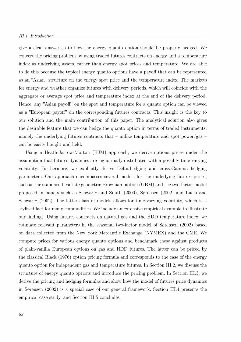
III.1. Introduction
give a clear answer as to how the energy quanto option should be properly hedged. We
convert the pricing problem by using traded futures contracts on energy and a temperature
index as underlying assets, rather than energy spot prices and temperature. We are able
to do this because the typical energy quanto options have a payoff that can be represented
as an ”Asian” structure on the energy spot price and the temperature index. The markets
for energy and weather organize futures with delivery periods, which will coincide with the
aggregate or average spot price and temperature index at the end of the delivery period.
Hence, any ”Asian payoff” on the spot and temperature for a quanto option can be viewed
as a ”European payoff” on the corresponding futures contracts. This insight is the key to
our solution and the main contribution of this paper. The analytical solution also gives
the desirable feature that we can hedge the quanto option in terms of traded instruments,
namely the underlying futures contracts that – unlike temperature and spot power/gas –
can be easily bought and held.
Using a Heath-Jarrow-Morton (HJM) approach, we derive options prices under the
assumption that futures dynamics are lognormally distributed with a possibly time-varying
volatility. Furthermore, we explicitly derive Delta-hedging and cross-Gamma hedging
parameters. Our approach encompasses several models for the underlying futures prices,
such as the standard bivariate geometric Brownian motion (GBM) and the two-factor model
proposed in papers such as Schwartz and Smith (2000), Sørensen (2002) and Lucia and
Schwartz (2002). The latter class of models allows for time-varying volatility, which is a
stylized fact for many commodities. We include an extensive empirical example to illustrate
our findings. Using futures contracts on natural gas and the HDD temperature index, we
estimate relevant parameters in the seasonal two-factor model of Sørensen (2002) based
on data collected from the New York Mercantile Exchange (NYMEX) and the CME. We
compute prices for various energy quanto options and benchmark these against products
of plain-vanilla European options on gas and HDD futures. The latter can be priced by
the classical Black (1976) option pricing formula and corresponds to the case of the energy
quanto option for independent gas and temperature futures. In Section III.2, we discuss the
structure of energy quanto options and introduce the pricing problem. In Section III.3, we
derive the pricing and hedging formulas and show how the model of futures price dynamics
in Sørensen (2002) is a special case of our general framework. Section III.4 presents the
empirical case study, and Section III.5 concludes.
88
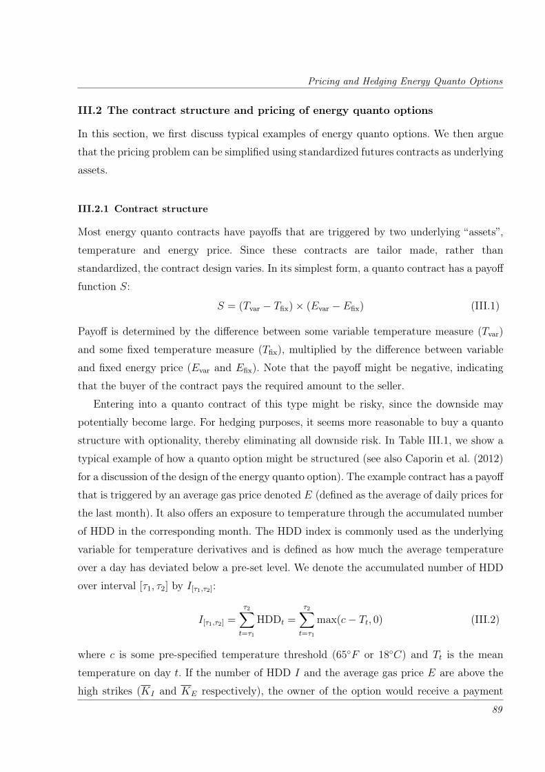
Pricing and Hedging Energy Quanto Options
III.2 The contract structure and pricing of energy quanto options
In this section, we first discuss typical examples of energy quanto options. We then argue
that the pricing problem can be simplified using standardized futures contracts as underlying
assets.
III.2.1 Contract structure
Most energy quanto contracts have payoffs that are triggered by two underlying “assets”,
temperature and energy price. Since these contracts are tailor made, rather than
standardized, the contract design varies. In its simplest form, a quanto contract has a payoff
function S:
S = (Tvar − Tfix)× (Evar − Efix) (III.1)
Payoff is determined by the difference between some variable temperature measure (Tvar)
and some fixed temperature measure (Tfix), multiplied by the difference between variable
and fixed energy price (Evar and Efix). Note that the payoff might be negative, indicating
that the buyer of the contract pays the required amount to the seller.
Entering into a quanto contract of this type might be risky, since the downside may
potentially become large. For hedging purposes, it seems more reasonable to buy a quanto
structure with optionality, thereby eliminating all downside risk. In Table III.1, we show a
typical example of how a quanto option might be structured (see also Caporin et al. (2012)
for a discussion of the design of the energy quanto option). The example contract has a payoff
that is triggered by an average gas price denoted E (defined as the average of daily prices for
the last month). It also offers an exposure to temperature through the accumulated number
of HDD in the corresponding month. The HDD index is commonly used as the underlying
variable for temperature derivatives and is defined as how much the average temperature
over a day has deviated below a pre-set level. We denote the accumulated number of HDD
over interval [τ1, τ2] by I[τ1,τ2]:
I[τ1,τ2] =
τ2∑t=τ1
HDDt =
τ2∑t=τ1
max(c− Tt, 0) (III.2)
where c is some pre-specified temperature threshold (65F or 18C) and Tt is the mean
temperature on day t. If the number of HDD I and the average gas price E are above the
high strikes (KI and KE respectively), the owner of the option would receive a payment
89
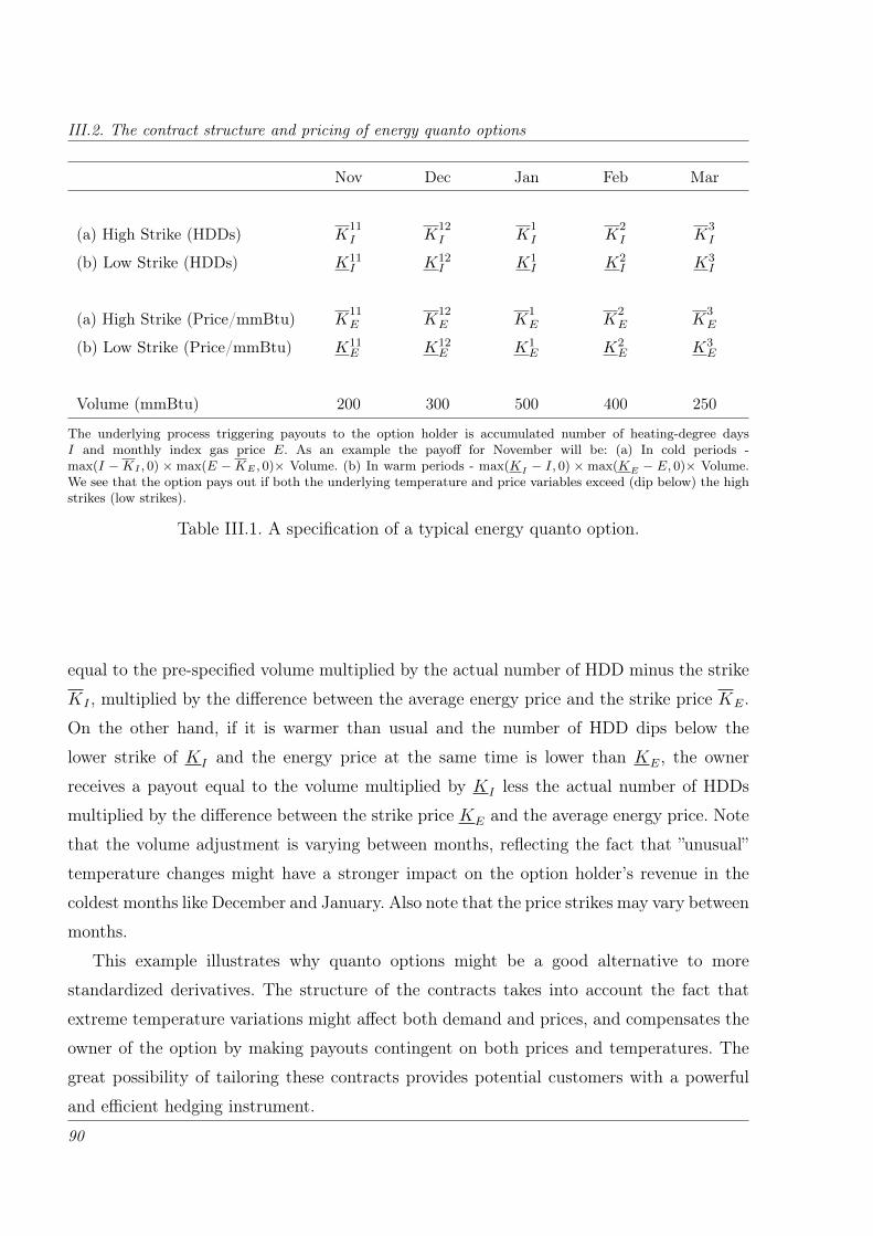
III.2. The contract structure and pricing of energy quanto options
Nov Dec Jan Feb Mar
(a) High Strike (HDDs) K11I K
12I K
1I K
2I K
3I
(b) Low Strike (HDDs) K11I K12
I K1I K2
I K3I
(a) High Strike (Price/mmBtu) K11E K
12E K
1E K
2E K
3E
(b) Low Strike (Price/mmBtu) K11E K12
E K1E K2
E K3E
Volume (mmBtu) 200 300 500 400 250
The underlying process triggering payouts to the option holder is accumulated number of heating-degree daysI and monthly index gas price E. As an example the payoff for November will be: (a) In cold periods -max(I −KI , 0) × max(E −KE , 0)× Volume. (b) In warm periods - max(KI − I, 0) × max(KE − E, 0)× Volume.We see that the option pays out if both the underlying temperature and price variables exceed (dip below) the highstrikes (low strikes).
Table III.1. A specification of a typical energy quanto option.
equal to the pre-specified volume multiplied by the actual number of HDD minus the strike
KI , multiplied by the difference between the average energy price and the strike price KE.
On the other hand, if it is warmer than usual and the number of HDD dips below the
lower strike of KI and the energy price at the same time is lower than KE, the owner
receives a payout equal to the volume multiplied by KI less the actual number of HDDs
multiplied by the difference between the strike price KE and the average energy price. Note
that the volume adjustment is varying between months, reflecting the fact that ”unusual”
temperature changes might have a stronger impact on the option holder’s revenue in the
coldest months like December and January. Also note that the price strikes may vary between
months.
This example illustrates why quanto options might be a good alternative to more
standardized derivatives. The structure of the contracts takes into account the fact that
extreme temperature variations might affect both demand and prices, and compensates the
owner of the option by making payouts contingent on both prices and temperatures. The
great possibility of tailoring these contracts provides potential customers with a powerful
and efficient hedging instrument.
90

Pricing and Hedging Energy Quanto Options
III.2.2 Pricing Using Terminal Value of Futures
As described above energy quanto options have a payoff which is a function of two underlying
assets, temperature and price. We focus on a class of energy quanto options which has
a payoff function f(E, I), where E is an index of the energy price and I an index of
temperature. To be more specific, we assume that the energy index E is given as the average
spot price over some measurement period [τ1, τ2]3, τ1 < τ2,
E =1
τ2 − τ1
τ2∑u=τ1
Su,
where Su denotes the energy spot price. Further, we assume that the temperature index is
defined as
I =
τ2∑u=τ1
g(Tu)
for Tu being the temperature at time u and g some function. For example, if we want to
consider a quanto option involving the HDD index, we choose g(x) = max(18 − x, 0). The
quanto option is exercised at time τ2, and its arbitrage-free price Ct at time t ≤ τ2 is defined
as by the following expression:
Ct = e−r(τ2−t)EQt
[f
(1
τ2 − τ1
τ2∑u=τ1
Su,
τ2∑u=τ1
g(Tu)
)]. (III.3)
Here, r > 0 denotes the risk-free interest rate, which we for simplicity assumes constant.
The pricing measure is denoted Q, and EQt [·] is the expectation operator with respect to Q,
conditioned on the market information at time t given by the filtration Ft.We now argue how to relate the price of the quanto option to futures contracts on the
energy and temperature indexes E and I. Observe that the price at time t ≤ τ2 of a futures
contract written on some energy price, (eg, natural gas) with delivery period [τ1, τ2] is given
by
FEt (τ1, τ2) = EQ
t
[1
τ2 − τ1
τ2∑u=τ1
Su
].
At time t = τ2, we find from the conditional expectation that
FEτ2
(τ1, τ2) =1
τ2 − τ1
τ2∑u=τ1
Su,
3Technically we should write τ2− τ1 + 1, when using the discretely computed average. To ease the notation, we keep
τ2 − τ1 to determine the average over the period.
91
III.2. The contract structure and pricing of energy quanto options
ie, the futures price is exactly equal to what is being delivered. Applying the same argument
to a futures written on the temperature index, with price dynamics denoted F It (τ1, τ2), we
immediately see that the following must be true for the quanto option price:
Ct = e−r(τ2−t)EQt
[f
(1
τ2 − τ1
τ2∑u=τ1
Su,
τ2∑u=τ1
g(Tu)
)]= e−r(τ2−t)EQ
t
[f(FEτ2
(τ1, τ2),F Iτ2
(τ1, τ2))]
. (III.4)
Equation (III.4) shows that the price of a quanto option with payoff being a function of
the energy index E and temperature index I must be the same as if the payoff was a function
of the terminal values of two futures contracts written on the energy and temperature
indexes, and with the delivery period being equal to the contract period specified by the
quanto option. Hence, we view the quanto option as an option written on the two futures
contracts, rather than on the two indexes. This is advantageous from the point of view
that the futures are traded financial assets. We note in passing that we may extend the
above argument to quanto options where the measurement periods of the energy and the
temperature indexes are not the same.
To compute the price in (III.4) we must have a model for the futures price dynamics
FEt (τ1, τ2) and F I
t (τ1, τ2). The dynamics must account for the dependency between the two
futures, as well as their marginal behaviour. The pricing of the energy quanto option has thus
been transferred from modelling the joint spot energy and temperature dynamics, followed
by computing theQ-expectation of an index of these, to modelling the joint futures dynamics
and pricing a European-type option on these. The former approach is similar to pricing an
Asian option, which for most relevant models and cases is a highly difficult task. Remark
also that by modelling and estimating the futures dynamics to market data, we can easily
obtain the market-implied pricing measure Q. We will see this in practice in Section III.4,
where we analyse the case of gas and HDD futures. If we choose to model the underlying
energy spot prices and temperature dynamics, one obtains the dynamics under the market
probability P, rather than under the pricing measure Q. Additional hypotheses must be
made in the model to obtain this. Moreover, for most interesting cases, the quanto option
must be priced by Monte Carlo or some other computationally demanding method (see
Caporin et al. (2012)). Finally, but no less importantly, with the representation in (III.4) at
hand we can discuss the issue of hedging energy quanto options in terms of the underlying
futures contracts.
92
Pricing and Hedging Energy Quanto Options
In many energy markets, the futures contracts are not traded within their delivery period.
That means that we can only use the market for futures up to time τ1. This has a clear
consequence on the possibility to hedge these contracts, as a hedging strategy inevitably
will be a continuously rebalanced portfolio of the futures up to the exercise time τ2. As
this is possible to perform only up to time τ1 in many markets, we face an incomplete
market situation where the quanto option cannot be hedged perfectly. Moreover, it is to
be expected that the dynamics of the futures price have different characteristics within the
delivery period than prior to start of delivery, if it can be traded for times t ∈ (τ1, τ2]. The
reason being that we have less uncertainty as the remaining delivery period of the futures
become shorter. In this paper we will restrict our attention to the pricing of quanto options
at times t ≤ τ1. The entry time of such a contract is most naturally taking place prior
to delivery period. However, for marking-to-market purposes, one is interested in the price
Ct also for t ∈ (τ1, τ2]. The issuer of the quanto option may be interested in hedging the
exposure, and therefore also be concerned of the behaviour of prices within the delivery
period.
Before we start looking into the details of pricing quanto options, we investigate the
option contract of the type described in section III.2.1 in more detail. This contract covers
a period of five months, from November through to March. Since this contract is essentially
a sum of one-period contracts, we focus our attention on an option covering only one month
of delivery period [τ1, τ2]. Recall that the payoff in the contract is a function of some average
energy price and accumulated number of HDD. From the discussion in the previous section
we know that rather than using spot price and HDD as underlying assets, we can instead use
the terminal value of futures contracts written on price and HDD, respectively. The payoff
function p(FEτ2
(τ1, τ2),F Iτ2
(τ1, τ2),KE,KI ,KE,KI) = p of this quanto contract is defined as
p = γ[max
(FEτ2
(τ1, τ2)−KE, 0)
max(F Iτ2
(τ1, τ2)−KI , 0)
+ max(KE − FE
τ2(τ1, τ2), 0
)max
(KI − F I
τ2(τ1, τ2), 0
)], (III.5)
where γ is the contractual volume adjustment factor. Note that the payoff function in this
contract consists of two parts, the first taking care of the situation in which temperatures
are colder (and prices higher) than usual, and the second taking care of the situation in
which temperatures are warmer than usual (and prices lower than usual). The first part is
a product of two call options, whereas the second part is a product of two put options. To
illustrate our pricing approach in the simplest possible way it suffices to look at the product
93
III.3. Asset Price Dynamics and Option Prices
call structure with the volume adjuster γ normalized to 1, ie, we want to price an option
with the following payoff function:
p(FEτ2
(τ1, τ2),F Iτ2
(τ1, τ2),KE,KI
)= max
(FEτ2
(τ1, τ2)−KE, 0) (F Iτ2
(τ1, τ2)−KI , 0)
.
(III.6)
In the remainder of this paper, we will focus on this particular choice of a payoff function
for the energy quanto option. It corresponds to choosing the function f as f(E, I) =
max(E − KE, 0) max(I − KI , 0) in (III.4). Other combinations of put-call mixes, as well
as different delivery periods for the energy and temperature futures can easily be studied
by a simple modification of what follows.
III.3 Asset Price Dynamics and Option Prices
Suppose that the two futures price dynamics under the pricing measure Q can be expressed
as
FET (τ1, τ2) = FE
t (τ1, τ2) exp(µE +X) (III.7)
F IT (τ1, τ2) = F I
t (τ1, τ2) exp(µI + Y ) (III.8)
where t ≤ T ≤ τ1, and X, Y are two random variables independent of Ft, but depending on
t,T , τ1 and τ2. We suppose that (X,Y ) is a bivariate normally distributed random variable
with mean zero. We define
σ2X = var(X), σ2
Y = var(Y ) and ρX,Y = cov(X,Y )
Obviously, σX ,σY and ρX,Y are depending on t,T , τ1 and τ2. Moreover, as the futures
price naturally is a martingale under the pricing measure Q, we have µE = −σ2X/2 and
µI = −σ2Y /2.
Our general representation of the futures price dynamics III.7 and III.8 encompasses
many interesting models. For example, a bivariate geometric Brownian motion looks like
FET (τ1, τ2) = FE
t (τ1, τ2) exp
(−1
2σ2E(T − t) + σE(WT −Wt)
)F IT (τ1, τ2) = F I
t (τ1, τ2) exp
(−1
2σ2I (T − t) + σI(BT −Bt)
)with two Brownian motionsW and B being correlated. We can easily associate this GBM to
the general set-up above by setting µE = −σ2E(T−t)/2, µI = −σ2
I (T−t)/2, σX = σE√T − t,
94
Pricing and Hedging Energy Quanto Options
σY = σI√T − t, and ρX,Y being the correlation between the two Brownian motions. In
section III.3.2, we show that also the two-factor model by Schwartz and Smith (2000) and
the extension by Sørensen (2002) fits this framework.
III.3.1 A General Solution for the Quanto Option Price and Hedge
The price of the quanto option at time t is
Ct = e−r(τ2−t)EQt
[p(FEτ2
(τ1, τ2),F Iτ2
(τ1, τ2),KE,KI
)](III.9)
where the notation EQ states that the expectation is taken under the pricing measure Q.
Given these assumptions, Proposition 1 below states the closed-form solution of the energy
quanto option.
Proposition III.1 For two assets following the dynamics given by (III.7) and (III.8), the
time t market price of an European energy quanto option with exercise at time τ2 and payoff
described by (III.6) is given by
Ct = e−r(τ2−t)(FEt (τ1, τ2)F I
t (τ1, τ2)eρX,Y σXσYM(y∗∗∗1 , y∗∗∗2 ; ρX,Y )
− FEt (τ1, τ2)KIM (y∗∗1 , y∗∗2 ; ρX,Y ) (III.10)
− F It (τ1, τ2)KEM (y∗1, y∗2; ρX,Y ) +KEKIM (y1, y2; ρX,Y )
)where
y1 =log(FE
t (τ1, τ2))− log(KE)− 12σ2X
σXy2 =
log(F It (τ1, τ2))− log(KI)− 1
2σ2Y
σY
y∗1 = y1 + ρX,Y σY y∗2 = y2 + σY
y∗∗1 = y1 + σX y∗∗2 = y2 + ρX,Y σX
y∗∗∗1 = y1 + ρX,Y σY + σX y∗∗∗2 = y2 + ρX,Y σX + σY
HereM(x, y; ρ) denotes the standard bivariate normal cumulative distribution function with
correlation ρ. 2
Proof: Observe that the payoff function in (III.6) can be rewritten in the following way:
p(FE,F I ,KE,KI) = max(FE −KE, 0) max(F I −KI , 0)
=(FE −KE
) (F I −KI
)1FE>KE1F I>KI
=FEF I1FE>KE1F I>KI − FEKI1FE>KE1F I>KI
− F IKE1FE>KE1F I>KI +KEKI1FE>KE1F I>KI
95
III.3. Asset Price Dynamics and Option Prices
The problem of finding the market price of the European quanto option is thus equivalent to
the problem of calculating the expectations under the pricing measure Q of the four terms
above. The four expectations are derived in Appendix III.A in details.
Based on III.10 we derive the Delta and cross-Gamma hedging parameters, which can be
straightforwardly calculated by partial differentiation of the price Ct with respect to the
futures prices. All hedging parameters are given by the current futures price of the two
underlying contracts and are therefore simple to implement in practice. The delta hedge
with respect to the energy futures is given by∂Ct
∂FEt (τ1, τ2)
= F It (τ1, τ2)e−r(τ2−t)+ρX,Y σXσY
(M (y∗∗∗1 , y∗∗∗2 ; ρX,Y ) +B(y∗∗∗1 )N(y∗∗∗2 − ρX,Y )
1
σX
)−KIe
−r(τ2−t)(M (y∗∗1 , y∗∗2 ; ρX,Y ) +B(y∗∗1 )N(y∗∗2 − ρX,Y )
1
σX
)− F I
t (τ1, τ2)KE
FEt (τ1, τ2)σX
e−r(τ2−t)B(y∗1)N(y∗2 − ρX,Y )
+KEKI
FEt (τ1, τ2)σX
e−r(τ2−t)B(y1)N(y2 − ρX,Y ) (III.11)
where N(·) denotes the standard normal cumulative distribution function, and
B(x) =e(x
2−ρ2X,Y )
4π2(1− ρ2
X,Y
)The Delta hedge with respect to the temperature index futures is of course analogous to
the energy Delta hedge, only with the substitutions FEt (τ1, τ2) = F I
t (τ1, τ2), y∗∗∗1 = y∗∗∗2 ,
y∗∗1 = y∗∗2 , y∗1 = y∗2, y1 = y2, σY = σX and σX = σY . The cross-Gamma hedge is given by
∂C2t
∂FEt (τ1, τ2)∂F I
t (τ1, τ2)
= e−r(τ2−t)+ρX,Y σXσY
(M (y∗∗∗1 , y∗∗∗2 ; ρX,Y ) +B(y∗∗∗2 )N(y∗∗∗1 − ρX,Y )
1
σY
)+ e−r(τ2−t)+ρX,Y σXσYB(y∗∗∗1 )
(N(y∗∗∗2 − ρX,Y )
1
σX+ n(y∗∗∗2 − ρX,Y )
1
σY
)− KI
F It (τ1, τ2)σY
e−r(τ2−t)(B(y∗∗2 )N(y∗∗1 − ρX,Y ) +B(y∗∗1 )n(y∗∗2 − ρX,Y )
1
σX
)− KE
FEt (τ1, τ2)σX
e−r(τ2−t)B(y∗1)
(N(y∗2 − ρX,Y ) + n(y∗2 − ρX,Y )
1
σY
)+
KEKI
FEt (τ1, τ2)F I
t (τ1, τ2)(σX + σY )e−r(τ2−t)B(y1)n(y2 − ρX,Y ) (III.12)
where n(·) denotes the standard normal probability density function (pdf). In our model
it is possible to hedge the quanto option perfectly, with positions described above by the
96

Pricing and Hedging Energy Quanto Options
three Delta and Gamma parameters. In practice, however, this would be difficult due to low
liquidity in, for example, the temperature market. Furthermore, as discussed in Section
III.2.2, we cannot in all markets trade futures within the delivery period, which puts
additional restrictions on the suitability of the hedge. In such cases, the parameters above
will guide in a partial hedging of the option.
III.3.2 Two-dimensional Schwartz-Smith Model with Seasonality
The popular commodity price model proposed by Schwartz and Smith (2000) is a natural
starting point for deriving dynamics of energy futures. In this model, the log-spot price is the
sum of two processes, one representing the long-term dynamics of the commodity prices in
form of an arithmetic Brownian motion and one representing the short term deviations from
the long run dynamics in the form of an Ornstein-Uhlenbeck process with a mean reversion
level of zero. Other papers such as Lucia and Schwartz (2002) and Sørensen (2002) uses
the same two driving factors and extends the model to include seasonality. We choose the
seasonality parametrization of the latter and further extend to a two-asset framework by
linking the driving Brownian motions. The dynamics under P is given by
logSt = Λ(t) +Xt + Zt
dXt =
(µ− 1
2σ2
)dt+ σdWt
dZt = −κZtdt+ νdBt
Here B and W are correlated Brownian motions and µ,σ,κ and η are constants. The
deterministic function Λ(t) describes the seasonality of the log-spot prices. In order to price
a futures contract written on an underlying asset with the above dynamics, a measure
change from P to an equivalent probability Q is made:
dXt =
(α− 1
2σ2
)dt+ σdWt
dZt = − (λZ + κZt) dt+ νdBt
Here, α = µ − λX , and λX and λZ are constant market prices of risk associated with Xt
and Zt respectively. This corresponds to a Girsanov transform of B and W by a constant
drift so that B and W become two correlated Q-Brownian motions. As is well-known for
the Girsanov transform, the correlation between B and W is the same under Q as the one
for B and W under P (see Karatzas and Shreve (2000)). Following Sørensen (2002), the
97
III.3. Asset Price Dynamics and Option Prices
futures price Ft(τ) at time t ≥ 0 of a contract with delivery at time τ ≥ t has the following
form on log scale (note that it is the Schwartz-Smith futures prices scaled by a seasonality
function):
logFt(τ) = Λ(τ) + A(τ − t) +Xt + Zte−κ(τ−t) (III.13)
where
A(τ) = ατ − λZ − ρσνκ
(1− e−κτ
)+ν2
4κ
(1− e−2κτ
).
The log futures prices are affine in the two factors X and Z driving the spot price and scaled
by functions of time to delivery τ−t and by functions of time of delivery, τ . Sørensen (2002)
chooses to parametrize the seasonality function Λ by a linear combination of cosine and sine
functions:
Λ(t) =K∑k=1
(γk cos(2πkt) + γ∗k sin(2πkt)) (III.14)
In this paper, we have highlighted the fact that the payoff of energy quanto options can
be expressed in terms of the futures prices of energy and temperature index. We can use
the above procedure to derive futures price dynamics from a model of the spot. However,
we can also state directly the futures price dynamics in the fashion of Heath-Jarrow-Morton
(HJM) using the above model as inspiration for the specification of the model. The HJM
approach was proposed to model energy futures by Clewlow and Strickland (2000), and
later investigated in detail by Benth and Koekebakker (2008) (see also Benth, Benth, and
Koekebakker (2008) and Miltersen and Schwartz (1998)). We follow this approach here,
proposing a joint model for the energy and temperature index futures price based on the
seasonal Schwartz-Smith model.
In stating such a model, we must account for the fact that the futures in question are
delivering over a period [τ1, τ2], and not at a fixed delivery time τ . An attractive alternative
to the additive approach by Lucia and Schwartz (2002), is to let Ft(τ1, τ2) itself follow a
dynamics of the form (III.13) with some appropriately chosen dependency on τ1 and τ2. For
example, we may choose τ = τ1 in (III.13), or τ = (τ1 + τ2)/2, or any other time within
the delivery period [τ1, τ2]. In this way, we will account for the delivery time-effect in the
futures price dynamics, sometimes referred to as the Samuelson effect. We remark that it
is well-known that, for futures delivering over a period, the volatility will not converge to
that of the underlying spot as time to delivery goes to zero (see Benth et al. (2008)). By
the above choices, we obtain such an effect.
98
Pricing and Hedging Energy Quanto Options
In order to jointly model the energy and temperature futures price, two futures dynamics
of the type in (III.13) are connected by allowing the Brownian motions to be correlated across
assets. We will have four Brownian motionsWE,BE,W I and BI in our two-asset, two-factor
model. These are assumed correlated as follows: ρE = corr(WE1 ,BE
1 ), ρI = corr(W I1 ,BI
1),
ρW = corr(WE1 ,W I
1 ) and ρB = corr(BE1 ,BI
1). Moreover, we have cross-correlations given by
ρW ,BI,E = corr(W I
1 ,BE1 )
ρW ,BE,I = corr(WE
1 ,BI1)
In a HJM-style, we assume that the joint dynamics of the futures price processes FEt (τ1, τ2)
and F It (τ1, τ2) under Q is given by
dF it (τ1, τ2)
F it (τ1, τ2)
= σidWit + ηi(t)dB
it (III.15)
for i = E, I and with
ηi(t) = νie−κi(τ2−t) (III.16)
Note that we suppose the futures price is a martingale with respect to the pricing measure
Q, which is natural from the point of view that we want an arbitrage-free model. Moreover,
we have made the explicit choice here that τ = τ2 in (III.13) when modelling the delivery
time effect. Note that
d logF it (τ1, τ2) = −1
2
(σ2i + ηi(t)
2 + 2ρiσiηi(t))dt+ σidW
it + ηi(t)dB
it
for i = E, I. Hence, we can make the representation FET (τ1, τ2) = FE
t (τ1, τ2) exp (−µE +X)
by choosing
X ∼ N(
0,
∫ T
t
(σ2E + ηE(s)2 + 2ρEσEηE(s)
)ds︸ ︷︷ ︸
σ2X
), µE = −1
2σ2X
and similarly for F IT (τ1, τ2). These integrals can be computed analytically in the above
model, where ηi(t) = νie−κi(τ2−t). We can also compute the correlation ρX,Y analytically,
since ρX,Y = cov(X,Y )σXσY
and
cov(X,Y ) = ρW
∫ T
t
σEσIds+ρW ,BE,I
∫ T
t
σEηI(s)ds+ρW ,BI,E
∫ T
t
ηE(s)σIds+ρB
∫ T
t
ηE(s)ηI(s)ds
99
III.4. Empirical Analysis
A closed-form expression of this covariance can be computed. In the special case of zero
cross-correlations this simplifies to
cov(X,Y ) = ρW
∫ T
t
σEσIds+ ρB
∫ T
t
ηE(s)ηI(s)ds
The exact expressions for σX , σY and cov(X,Y ) in the two-dimensional Schwartz-Smith
model with seasonality are presented in Appendix III.B.
This bivariate futures price model has a form that can be immediately used for pricing
energy quanto options by inferring the result in Proposition 1. We shall come back to this
model in the empirical case study in Section III.4. The general setup in section III.3 above
includes in fact the implied forward dynamics from general multi-factor spot models, with
stationary and non-stationary terms. Hence, this is a very general pricing mechanism, where
the basic essential problem is to identify the overall volatilities σX and σY , and the cross-
correlation ρX,Y . As a final remark, we note that our pricing approach only looks at futures
dynamics up to the start of the delivery period τ1. As briefly discussed in Section III.3.2 it is
reasonable to expect that the dynamics of a futures contract should be different within the
delivery period [τ1, τ2]. For times t within [τ1, τ2] we will, in the case of the energy futures,
have
Ft(τ1, τ2) =1
τ2 − τ1
t∑u=τ1
Su + EQt
[1
τ2 − τ1
τ2∑u=t+1
Su
].
Thus, the futures price must consist of two parts, the first simply the observed energy spot
prices up to time t, and next the second the current futures price of a contract with delivery
period [t, τ2]. This latter part will have a volatility that must go to zero as t tends towards
τ2.
III.4 Empirical Analysis
In this section, we present an empirical study of energy quanto options written on NYMEX
natural gas futures and the Heating Degree Days temperature index. We present the futures
price data which constitute the basis of our analysis, and estimate the parameters in the
joint futures price model (III.15). We then discuss the impact of correlation on the valuation
of the option to be priced.
100

Pricing and Hedging Energy Quanto Options
III.4.1 Data
Futures contracts for delivery of gas are traded on NYMEX for each month ten years out.
The underlying is delivery of gas throughout a month and the price is per unit. The contract
trades until a couple of days before the delivery month. Many contracts are closed prior to
the last trading day, and we choose the first 12 contracts for delivery at least one month
later. For example, for January 2 2007, we use March 2007 to February 2008 contracts.
We denote the time-t futures price for a contract delivering one month (= ∆) up till τ2 by
FEt ([τ2−∆, τ2]) and let the price follow a process of the type (III.13) discussed in the section
III.3.2. When investigating data, there is a seasonality pattern over the year, where prices,
in general, are lowest in late spring and early fall, slightly higher in between these periods
and highest in the winter. These two ”peaks” during the year are modelled by setting K = 2
in equation (III.14) similar to the seasonal pattern of the commodities studied in Sørensen
(2002). The choice is statistically supported by the significance of parameter estimates and
standard errors for the γ’s. The evolution of the futures gas curves is shown in Figure III.1.
Futures contracts on accumulated HDD are traded on CME for several cities for the
months October, November, December, January, February, March, and April, a couple of
years out. The contract value is $20 for the number HDD accumulated over the month for
a specific location, ie, a day with temperature is 60F adds 5 to the index and thereby $100
to the final settlement, whereas a day with temperature is 70F does not add to or subtract
from the index. The contract trades until the beginning of the concurrent month. The
futures price is denoted by F It (τ2−∆, τ2) and settled on the accumulated index,
∑HDDu.
Liquidity is basically non-existent after the first year, so for every day we choose the first
seven contracts, where the index period has not yet started, ie, for January 2, 2007, we use
the February 2007, March 2007, April 2007, October 2007, November 2007, December 2007
and January 2008 contracts.
Again, we let the futures price follow a price process of the type (III.13). The stationary
part represents the short term random fluctuations in the underlying temperature deviation.
Over a long time, we might argue that temperature and thereby a month of accumulated
HDD has a long term drift, but during the time period our data covers, the effect of
long-term environmental changes are negligible. The short time period covered speaks
justifies leaving out the nonstationary part, X. However, estimation of the full model led
to significant parameter estimates for σI (see Section III.4.2), so we choose to keep the
101
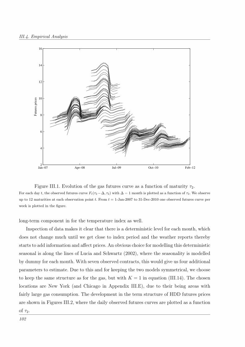
III.4. Empirical Analysis
Jan−07 Apr−08 Jul−09 Oct−10 Feb−122
4
6
8
10
12
14
16
Futu
res
pri
ces
Figure III.1. Evolution of the gas futures curve as a function of maturity τ2.For each day t, the observed futures curve Ft(τ2−∆, τ2) with ∆ = 1 month is plotted as a function of τ2. We observe
up to 12 maturities at each observation point t. From t = 1-Jan-2007 to 31-Dec-2010 one observed futures curve per
week is plotted in the figure.
long-term component in for the temperature index as well.
Inspection of data makes it clear that there is a deterministic level for each month, which
does not change much until we get close to index period and the weather reports thereby
starts to add information and affect prices. An obvious choice for modelling this deterministic
seasonal is along the lines of Lucia and Schwartz (2002), where the seasonality is modelled
by dummy for each month. With seven observed contracts, this would give us four additional
parameters to estimate. Due to this and for keeping the two models symmetrical, we choose
to keep the same structure as for the gas, but with K = 1 in equation (III.14). The chosen
locations are New York (and Chicago in Appendix III.E), due to their being areas with
fairly large gas consumption. The development in the term structure of HDD futures prices
are shown in Figures III.2, where the daily observed futures curves are plotted as a function
of τ2.
102
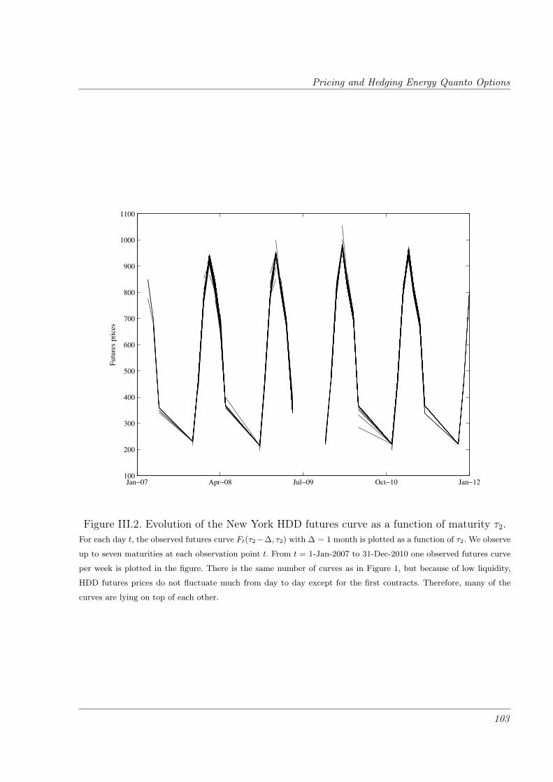
Pricing and Hedging Energy Quanto Options
Jan−07 Apr−08 Jul−09 Oct−10 Jan−12100
200
300
400
500
600
700
800
900
1000
1100
Futu
res
pri
ces
Figure III.2. Evolution of the New York HDD futures curve as a function of maturity τ2.For each day t, the observed futures curve Ft(τ2−∆, τ2) with ∆ = 1 month is plotted as a function of τ2. We observe
up to seven maturities at each observation point t. From t = 1-Jan-2007 to 31-Dec-2010 one observed futures curve
per week is plotted in the figure. There is the same number of curves as in Figure 1, but because of low liquidity,
HDD futures prices do not fluctuate much from day to day except for the first contracts. Therefore, many of the
curves are lying on top of each other.
103
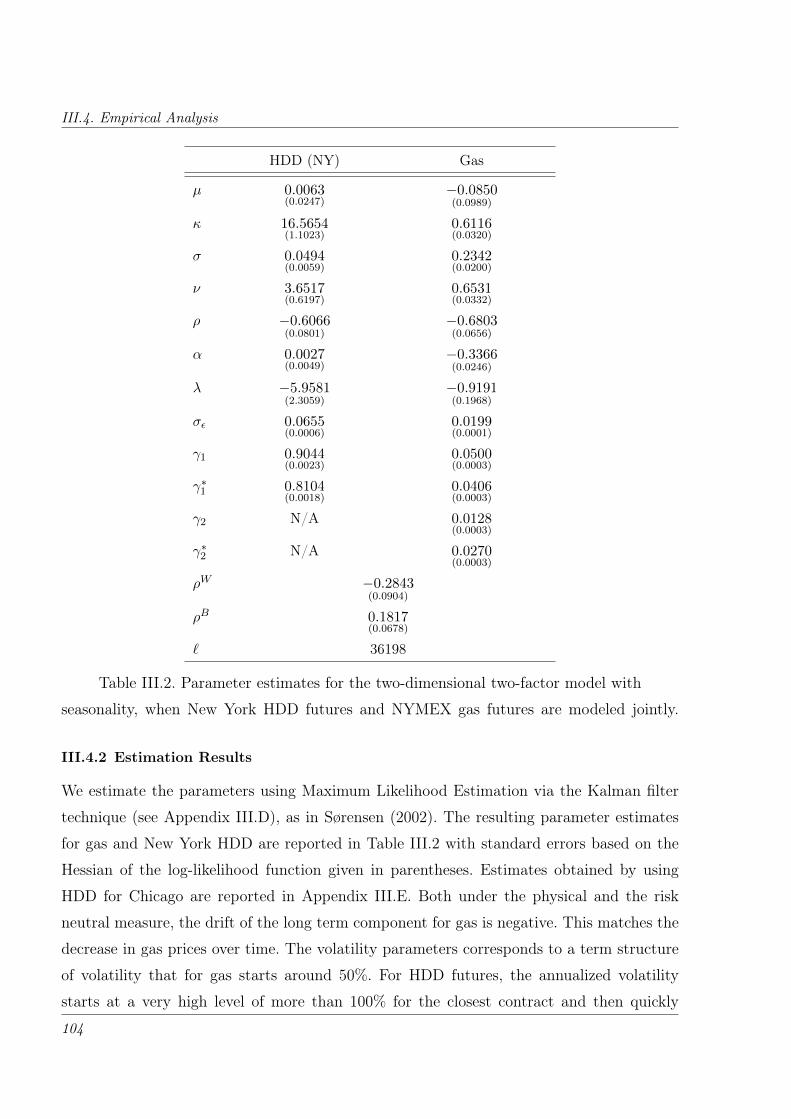
III.4. Empirical Analysis
HDD (NY) Gas
µ 0.0063(0.0247)
−0.0850(0.0989)
κ 16.5654(1.1023)
0.6116(0.0320)
σ 0.0494(0.0059)
0.2342(0.0200)
ν 3.6517(0.6197)
0.6531(0.0332)
ρ −0.6066(0.0801)
−0.6803(0.0656)
α 0.0027(0.0049)
−0.3366(0.0246)
λ −5.9581(2.3059)
−0.9191(0.1968)
σε 0.0655(0.0006)
0.0199(0.0001)
γ1 0.9044(0.0023)
0.0500(0.0003)
γ∗1 0.8104(0.0018)
0.0406(0.0003)
γ2 N/A 0.0128(0.0003)
γ∗2 N/A 0.0270(0.0003)
ρW −0.2843(0.0904)
ρB 0.1817(0.0678)
` 36198
Table III.2. Parameter estimates for the two-dimensional two-factor model with
seasonality, when New York HDD futures and NYMEX gas futures are modeled jointly.
III.4.2 Estimation Results
We estimate the parameters using Maximum Likelihood Estimation via the Kalman filter
technique (see Appendix III.D), as in Sørensen (2002). The resulting parameter estimates
for gas and New York HDD are reported in Table III.2 with standard errors based on the
Hessian of the log-likelihood function given in parentheses. Estimates obtained by using
HDD for Chicago are reported in Appendix III.E. Both under the physical and the risk
neutral measure, the drift of the long term component for gas is negative. This matches the
decrease in gas prices over time. The volatility parameters corresponds to a term structure
of volatility that for gas starts around 50%. For HDD futures, the annualized volatility
starts at a very high level of more than 100% for the closest contract and then quickly
104
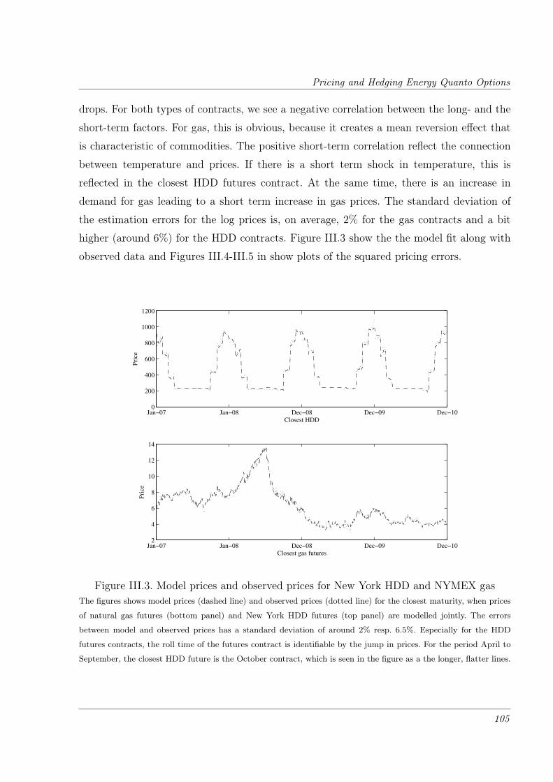
Pricing and Hedging Energy Quanto Options
drops. For both types of contracts, we see a negative correlation between the long- and the
short-term factors. For gas, this is obvious, because it creates a mean reversion effect that
is characteristic of commodities. The positive short-term correlation reflect the connection
between temperature and prices. If there is a short term shock in temperature, this is
reflected in the closest HDD futures contract. At the same time, there is an increase in
demand for gas leading to a short term increase in gas prices. The standard deviation of
the estimation errors for the log prices is, on average, 2% for the gas contracts and a bit
higher (around 6%) for the HDD contracts. Figure III.3 show the the model fit along with
observed data and Figures III.4-III.5 in show plots of the squared pricing errors.
Jan−07 Jan−08 Dec−08 Dec−09 Dec−100
200
400
600
800
1000
1200
Closest HDD
Pri
ce
Jan−07 Jan−08 Dec−08 Dec−09 Dec−102
4
6
8
10
12
14
Closest gas futures
Pri
ce
Figure III.3. Model prices and observed prices for New York HDD and NYMEX gasThe figures shows model prices (dashed line) and observed prices (dotted line) for the closest maturity, when prices
of natural gas futures (bottom panel) and New York HDD futures (top panel) are modelled jointly. The errors
between model and observed prices has a standard deviation of around 2% resp. 6.5%. Especially for the HDD
futures contracts, the roll time of the futures contract is identifiable by the jump in prices. For the period April to
September, the closest HDD future is the October contract, which is seen in the figure as a the longer, flatter lines.
105
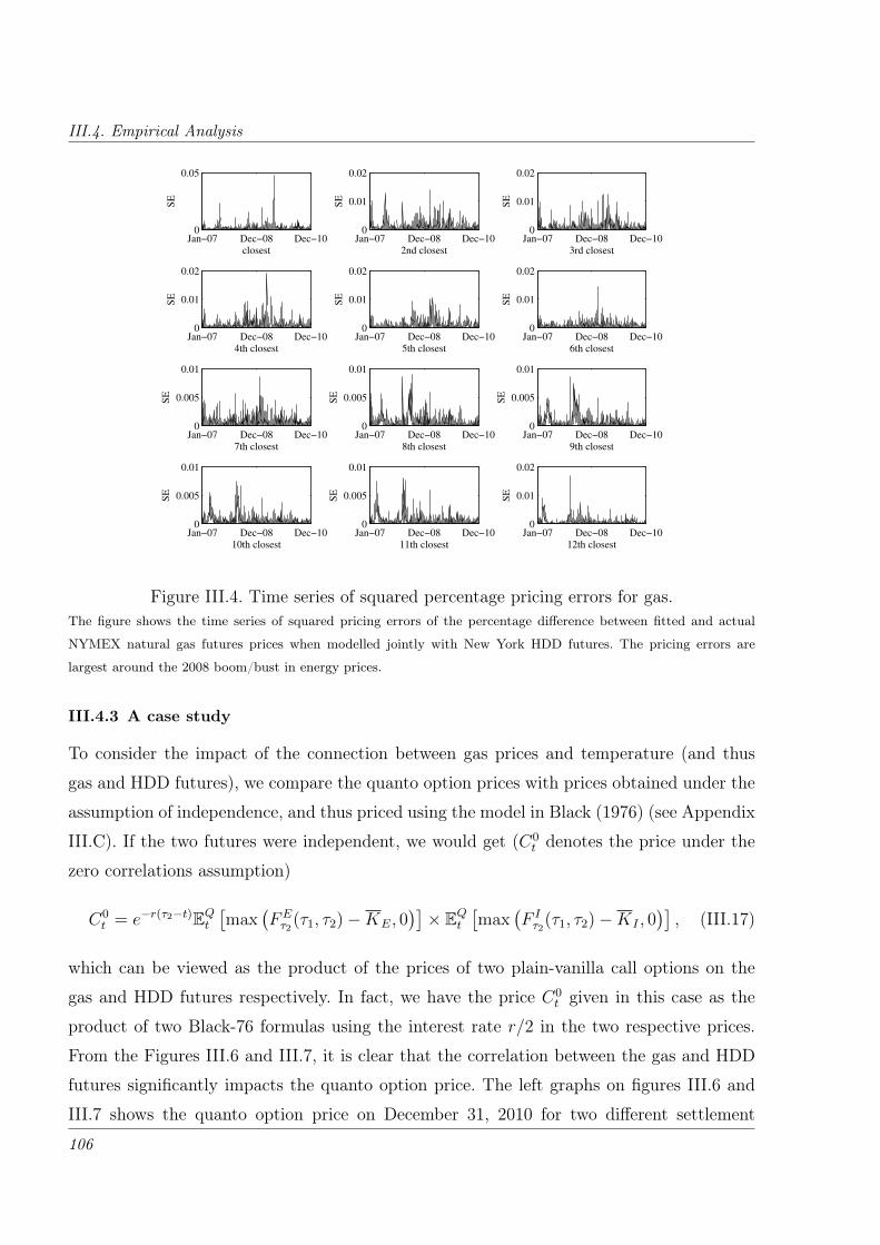
III.4. Empirical Analysis
Jan−07 Dec−08 Dec−100
0.05
closest
SE
Jan−07 Dec−08 Dec−100
0.01
0.02
2nd closest
SE
Jan−07 Dec−08 Dec−100
0.01
0.02
3rd closest
SE
Jan−07 Dec−08 Dec−100
0.01
0.02
4th closest
SE
Jan−07 Dec−08 Dec−100
0.01
0.02
5th closest
SE
Jan−07 Dec−08 Dec−100
0.01
0.02
6th closest
SE
Jan−07 Dec−08 Dec−100
0.005
0.01
7th closest
SE
Jan−07 Dec−08 Dec−100
0.005
0.01
8th closest
SE
Jan−07 Dec−08 Dec−100
0.005
0.01
9th closest
SE
Jan−07 Dec−08 Dec−100
0.005
0.01
10th closest
SE
Jan−07 Dec−08 Dec−100
0.005
0.01
11th closest
SE
Jan−07 Dec−08 Dec−100
0.01
0.02
12th closest
SE
Figure III.4. Time series of squared percentage pricing errors for gas.The figure shows the time series of squared pricing errors of the percentage difference between fitted and actual
NYMEX natural gas futures prices when modelled jointly with New York HDD futures. The pricing errors are
largest around the 2008 boom/bust in energy prices.
III.4.3 A case study
To consider the impact of the connection between gas prices and temperature (and thus
gas and HDD futures), we compare the quanto option prices with prices obtained under the
assumption of independence, and thus priced using the model in Black (1976) (see Appendix
III.C). If the two futures were independent, we would get (C0t denotes the price under the
zero correlations assumption)
C0t = e−r(τ2−t)EQt
[max
(FEτ2
(τ1, τ2)−KE, 0)]× EQt
[max
(F Iτ2
(τ1, τ2)−KI , 0)]
, (III.17)
which can be viewed as the product of the prices of two plain-vanilla call options on the
gas and HDD futures respectively. In fact, we have the price C0t given in this case as the
product of two Black-76 formulas using the interest rate r/2 in the two respective prices.
From the Figures III.6 and III.7, it is clear that the correlation between the gas and HDD
futures significantly impacts the quanto option price. The left graphs on figures III.6 and
III.7 shows the quanto option price on December 31, 2010 for two different settlement
106

Pricing and Hedging Energy Quanto Options
Jan−07 Jan−08 Dec−08 Dec−09 Dec−100
0.02
0.04
7th closest
SE
Jan−07 Jan−08 Dec−08 Dec−09 Dec−100
0.02
0.04
6th closest
SE
Jan−07 Jan−08 Dec−08 Dec−09 Dec−100
0.02
0.04
5th closest
SE
Jan−07 Jan−08 Dec−08 Dec−09 Dec−100
0.02
0.04
4th closest
SE
Jan−07 Jan−08 Dec−08 Dec−09 Dec−100
0.02
0.04
3rd closest
SE
Jan−07 Jan−08 Dec−08 Dec−09 Dec−100
0.02
0.04
2nd closest
SE
Jan−07 Jan−08 Dec−08 Dec−09 Dec−100
0.02
0.04
closest
SE
Figure III.5. Time series of squared percentage pricing errors for New York HDD.The figure shows the time series of squared pricing errors of the percentage difference between fitted and actual New
York HDD futures prices when modelled jointly with NYMEX natural gas futures. The pricing errors jump when
the contract roll.
months; December 2011 and February 2011 respectively. The right graphs on figures III.6
and III.7 shows the relative pricing error between the quanto option price with and without
correlation across assets. The ratio of the change in quanto option price to the product of the
marginal options, ie, (Ct−C0t )/Ct is plotted. For a short time to maturity, we see a relative
pricing error of more than 75% for the high strikes. The fact that the observed correlation
increases the quanto option price compared with the product of the two marginal options
indicates that more probability mass lies in the quanto’s exercise region. For short time to
maturity especially, ignoring correlation can lead to significant underpricing of the quanto
option.
III.5 Concluding remarks
In this paper, we presented a closed-form pricing formula for an energy quanto option under
the assumption that the underlying assets were lognormal. Taking advantage of the fact
that energy and temperature futures are designed with a delivery period, we showed how
107
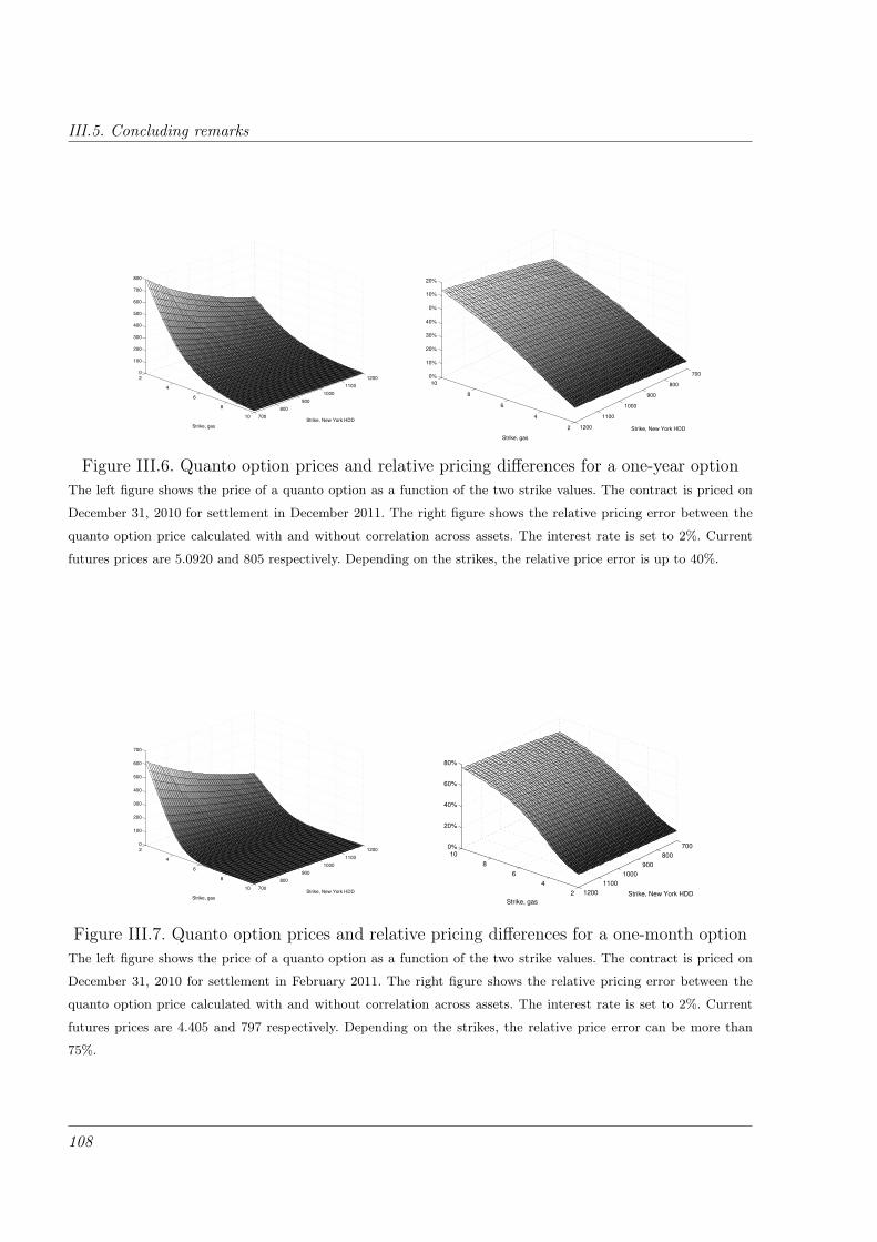
III.5. Concluding remarks
2
4
6
8
10 700
800
900
1000
1100
12000
100
200
300
400
500
600
700
800
Strike, New York HDD
Strike, gas 2
4
6
8
10
700
800
900
1000
1100
1200
0%
10%
20%
30%
40%
0%
10%
20%
Strike, New York HDD
Strike, gas
Figure III.6. Quanto option prices and relative pricing differences for a one-year optionThe left figure shows the price of a quanto option as a function of the two strike values. The contract is priced on
December 31, 2010 for settlement in December 2011. The right figure shows the relative pricing error between the
quanto option price calculated with and without correlation across assets. The interest rate is set to 2%. Current
futures prices are 5.0920 and 805 respectively. Depending on the strikes, the relative price error is up to 40%.
2
4
6
8
10 700
800
900
1000
1100
12000
100
200
300
400
500
600
700
Strike, New York HDD
Strike, gas2
4
6
8
10
700
800
900
1000
1100
1200
0%
20%
40%
60%
80%
Strike, New York HDD
Strike, gas
Figure III.7. Quanto option prices and relative pricing differences for a one-month optionThe left figure shows the price of a quanto option as a function of the two strike values. The contract is priced on
December 31, 2010 for settlement in February 2011. The right figure shows the relative pricing error between the
quanto option price calculated with and without correlation across assets. The interest rate is set to 2%. Current
futures prices are 4.405 and 797 respectively. Depending on the strikes, the relative price error can be more than
75%.
108
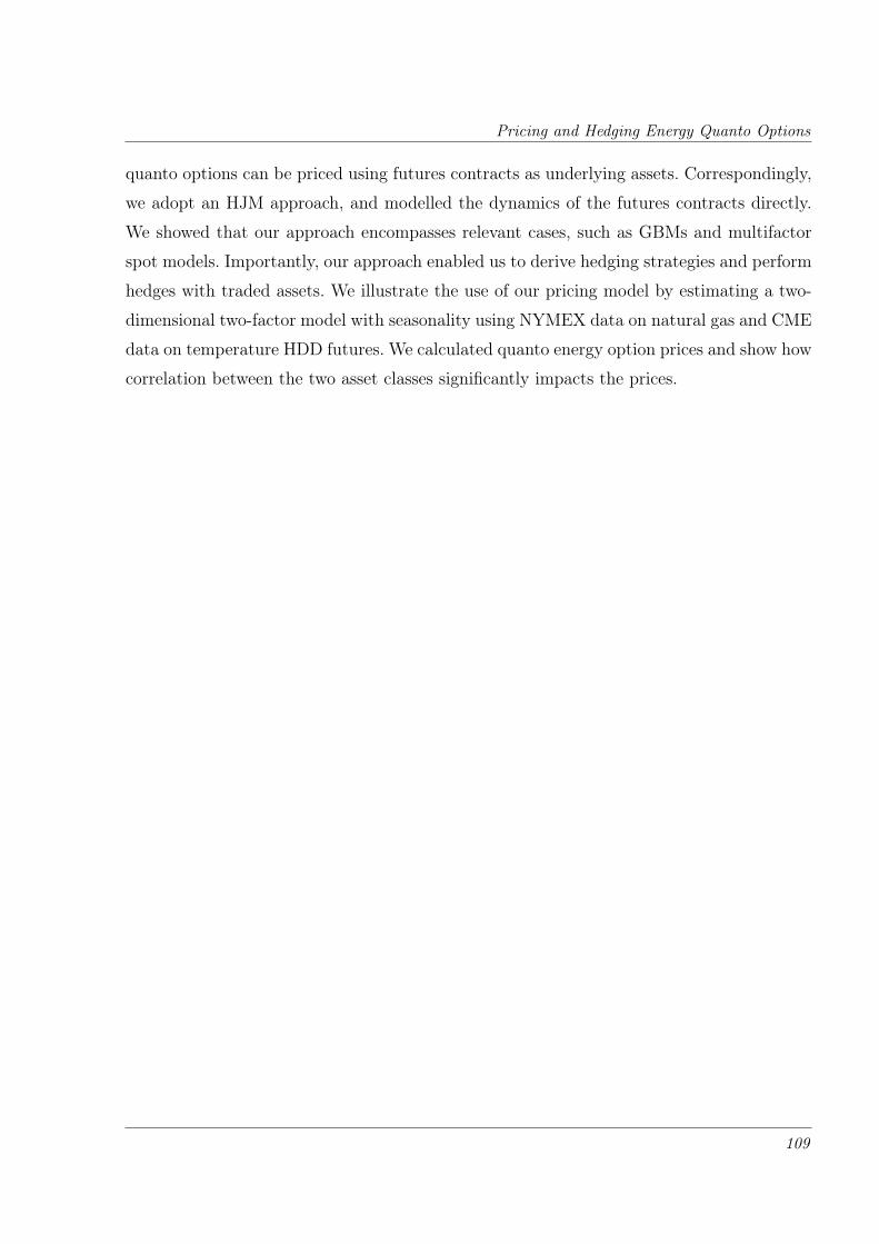
Pricing and Hedging Energy Quanto Options
quanto options can be priced using futures contracts as underlying assets. Correspondingly,
we adopt an HJM approach, and modelled the dynamics of the futures contracts directly.
We showed that our approach encompasses relevant cases, such as GBMs and multifactor
spot models. Importantly, our approach enabled us to derive hedging strategies and perform
hedges with traded assets. We illustrate the use of our pricing model by estimating a two-
dimensional two-factor model with seasonality using NYMEX data on natural gas and CME
data on temperature HDD futures. We calculated quanto energy option prices and show how
correlation between the two asset classes significantly impacts the prices.
109
III.A. Proof of pricing formula
Appendix
III.A Proof of pricing formula
In Section III.3.1 we showed that the payoff function in (III.6) could be rewritten in the
following way:
p(FET ,F I
T ,KI ,KE) = max(F IT −KI , 0) ·max(FE
T −KE, 0)
=(FET −KE
)·(F IT −KI
)· 1FET >KE · 1F IT>KI
= FET F
IT · 1FET >KE · 1F IT>KI − F
ET KI · 1FET >KE · 1F IT>KI
− F ITKE · 1FET >KE · 1F IT>KI +KEKI · 1FET >KE · 1F IT>KI.
Now, let us calculate the expectation under Q of the payoff function, ie,
EQt
[p(FE
T ,F IT ,KI ,KE)
]. We have
EQt
[p(FE
T ,F IT ,KI ,KE)
]= EQ
t
[max(F I
T −KI , 0) ·max(FET −KE, 0)
]= EQ
t
[FET F
IT1FET >KE1F IT>KI
]− EQ
t
[FET KI1FET >KE1F IT>KI
]− EQ
t
[F ITKE1FET >KE1F IT>KI
]+ EQ
t
[KEKI1FET >KE1>KI
].
(III.18)
In order to calculate the four different expectation terms we will use the same trick as
Zhang (1995), namely to rewrite the pdf of the bivariate normal distribution in terms of the
marginal pdf of the first variable times the conditional pdf of the second variable given the
first variable. Remember that we assume FET and F I
T to be lognormally distributed under
Q (ie, (X,Y ) are bivariate normal):
FET = FE
t eµE+X (III.19)
F IT = F I
t eµI+Y (III.20)
110

Pricing and Hedging Energy Quanto Options
where σ2X denotes variance of X, σ2
Y denotes variance of Y , and they are correlated by ρX,Y .
Consider the fourth expectation term first:
EQt
[KEKI1FET >KE1F IT>KI
]= KEKIEQ
t
[1FET >KE1F IT>KI
]= KEKIQt
(FET > KE
∩F IT > KI
)= KEKIQt
(FEt e
µE+X > KE
∩F It e
µI+Y > KI
)= KEKIQt
(X > log
(KE
FEt
)− µE
∩Y > log
(KI
F It
)− µI
)= KEKIQt
(−X < log
(FEt
KE
)+ µE
∩−Y < log
(F It
KI
)+ µI
)= KEKI ·M (y1, y2; ρX,Y )
where (ε1, ε2) are standard bivariate normal with correlation ρX,Y and
y1 =log(FEtKE
)+ µE
σXand y2 =
log(F ItKI
)+ µI
σY.
Next, consider the third expectation term,
EQt
[F ITKE1FET >KE1F IT>KI
]= F I
t KEeµIE
[eY 1FET >KE1F IT>KI
]= F I
t KEeµIE
[eσY ε21ε1<y11ε2<y2
]= F I
t KEeµI
∫ y2
−∞
∫ y1
−∞eσY ε2f (ε1, ε2) dε1dε2
= F It KEe
µI
∫ y2
−∞
∫ y1
−∞eσY ε2f (ε2) f (ε1|ε2) dε1dε2
= F It KEe
µI
∫ y2
−∞
∫ y1
−∞eσY ε2
1√2π
exp
(−1
2ε22
)×
1√
2π√
1− ρ2X,Y
exp
[−1
2(1− ρ2X,Y )
(ε1 − ρX,Y ε2)2
]dε1dε2.
(III.21)
Using the substitution w = −ε1 + ρε1,ε2σY and z = −ε2 + σY , the exponent in the above
expression becomes:
σY ε2 −1
2ε22 −
1
2(1− ρ2X,Y )
(ε21 + ρ2
X,Y ε22 − 2ρX,Y ε1ε2
)= − 1
2(1− ρ2X,Y )
(−2σY (1− ρ2
X,Y )ε2 + (1− ρ2X,Y )ε22 + ε21 + ρ2
X,Y ε22 − 2ρX,Y ε1ε2
)111
III.A. Proof of pricing formula
= − 1
2(1− ρ2X,Y )
(ε21 − 2σY (1− ρ2
X,Y )ε2 + ε22 − 2ρX,Y ε1ε2)
= − 1
2(1− ρ2X,Y )
(w2 + z2 − 2ρX,Y zw − (1− ρ2
X,Y )σ2Y
)= − 1
2(1− ρ2X,Y )
(w2 + z2 − 2ρX,Y zw
)+σ2Y
2,
which enable us to rewrite (III.21) as
EQt
[F ITKE1FET >KE1F IT>KI
]=
F It KEe
µI+σ2Y2
∫ y∗2
−∞
∫ y∗1
−∞
1
2π√
1− ρ2X,Y
exp
[− 1
2(1− ρ2X,Y )
(w2 + z2 − 2ρX,Y zw
)]dwdz
= F It KEe
µI+σ2Y2 M (y∗1, y∗2; ρX,Y )
where
y∗1 = y1 + ρX,Y σY and y∗2 = y2 + σY .
The second expectation term can be calculated in the same way as we calculated the
third term. The only difference is that we now use the substitution w = −ε1 + σX and
z = −ε2 + ρX,Y σX , so we can write
EQt
[FET KI1FET >KE1F IT>KI
]=
FEt KIe
µE+σ2X2
∫ y∗∗2
−∞
∫ y∗∗1
−∞
1
2π√
1− ρ2X,Y
exp
[− 1
2(1− ρ2X,Y )
(w2 + z2 − 2ρX,Y zw
)]dwdz
= FEt KIe
µE+σ2X2 M (y∗∗1 , y∗∗2 ; ρX,Y )
where
y∗∗1 = y1 + σX and y∗∗2 = y2 + ρX,Y σX .
Finally, consider the first expectation term in (III.18),
EQt
[FET F
IT1FET >KE1F IT>KI
]= FE
t FIt e
µE+µIEQt
[eX+Y 1FET >KE1F IT>KI
]= FE
t FIt e
µE+µIEQt
[eσXε1+σY ε21ε1<y11ε2<y2
]= FE
t FIt e
µE+µI
∫ y1
−∞
∫ y2
−∞eσXε1+σY ε2f(ε1, ε2)dε2dε1 (III.22)
Using the same trick as before with the substitution u = −ε1 + ρX,Y σY + σX and
v = −ε2 + ρX,Y σX + σY , expression (III.22) can be written
112
Pricing and Hedging Energy Quanto Options
EQt
[FET F
IT1FET >KE1F IT>KI
]= FE
t FIt e
µE+µI+ 12
(σ2X+σ2
Y +2ρX,Y σXσY )M(y∗∗∗1 , y∗∗∗2 ; ρX,Y )
(III.23)
where
y∗∗∗1 = y1 + ρX,Y σY + σX and y∗∗∗2 = y2 + ρX,Y σX + σY .
Thus, the expectation of the payoff function is
EQt
[p(FE
T ,F IT ,KI ,KE)
]= FE
t FIt e
µE+µI+ 12
(σ2X+σ2
Y +2ρX,Y σXσY )M(y∗∗∗1 , y∗∗∗2 ; ρX,Y )
− FEt KIe
µE+σ2X2 M (y∗∗1 , y∗∗2 ; ρX,Y )
− F It KEe
µI+σ2Y2 M (y∗1, y∗2; ρX,Y )
+KEKI ·M (y1, y2; ρX,Y ) .
Discounting the expected payoff gives us the price of the option.
III.B Closed-form solution for σ and ρ in the two-dimensional Schwartz-Smith
model with seasonality
σ2X =
∫ T
t
(σ2E +
(νEe
−κE(τ−s))2
+ 2ρEσE
(νEe
−κE(τ−s)))
ds
= σ2E(T − t) + νE
∫ T
t
e−2κE(τ−s)ds+ 2ρEσEνE
∫ T
t
e−κE(τ−s)ds
= σ2E(T − t) +
νE2κE
e−2κEτ(e2κET − e2κEt
)+ 2
ρEσEνEκE
e−κEτ(eκ
ET − eκEt)
;
cov(X,Y ) = ρW
∫ T
t
σEσIds+ ρB
∫ T
t
(νEe
−κE(τ−s))(
νIe−κI(τ−s)
)ds
= ρWσEσI(T − t) + ρBνEνIe−(κE+κI)τ
∫ T
t
e(κE+κI)sds
= ρWσEσI(T − t) +ρBνEνIκE + κI
e−(κE+κI)τ(e(κE+κI)T − e(κE+κI)t
);
ρX,Y =cov(X,Y )
σXσY.
When T = τ , this simplifies to
σX = σ2E(τ − t) +
νE2κE
(1− e−2κE(τ−t)
)+ 2
ρEσEνEκE
(1− eκE(τ−t)
),
ρX,Y =ρWσEσI(τ − t) + ρBνEνI
κE+κI
(1− e−(κE+κI)(τ−t)
)σXσY
.
113
III.C. One-dimensional option prices
III.C One-dimensional option prices
In this section, option prices on one underlying is presented. As for the joint case, assume
that the dynamics of a gas futures contract is given by:
FET (τ1, τ2) = FE
t (τ1, τ2) exp(µE +X).
Consider now a call option written on gas futures only. The price ct of this option is then
given by the Black (1976) formula, i.e.
ct = e−r(T−t) [FN(d1)−KN(d2)] ,
where
d1 =ln
FEtKE− µE
σX, d2 =
lnFEtKE
+ µE
σX.
The same formula of course applies to an option written only on temperature futures.
III.D Estimation using Kalman filter techniques
Given a set of observed futures prices, it is possible to estimate the parameters using Kalman
filter techniques. Let
Yn =(f Itn(T 1n
), . . . , f Itn
(TM
In
n
), fEtn
(T 1n
), . . . , fEtn
(TM
En
n
))′denote the set of log futures prices observed at time tn with maturities T 1
n , . . . ,TMIn
n for the
temperature contracts and maturities T 1n , . . . ,T
MEn
n for the gas contracts. The measurement
equation relates the observations to the unobserved state vector Un = (Xtn ,Ztn)′ by
Yn = dn + CnUn + εn
where the ε’s are measurement errors assumed iid normal with zero mean and covariance
matrix Hn. In the present framework we have
dn =
ΛI (T 1n) + AI (T 1
n − tn)...
ΛI(TMIn
n
)+ AI
(TMIn
n − tn)
ΛE (T 1n) + AE (T 1
n − tn)...
ΛE(TMEn
n
)+ AE
(TMEn
n − tn)
,Cn =
1 e−κI(T 1
n−tn)
......
1 e−κI
(TMIn
n −tn)
1 e−κE(T 1
n−tn)
......
1 e−κE
(TMEn
n −tn)
114
Pricing and Hedging Energy Quanto Options
and Hn =
(σ2ε,IIMI
n0
0 σ2ε,EIME
n
)The state-vector evolves according to
Un = c+ TUn + ηn
where ηn are i.i.d. normal with zero-mean vector and covariance matrix Q and where
c =
µI − 1
2
(σI)2
0
µE − 12
(σE)2
0
, ∆n+1, T =
1 0 0 0
0 e−κI∆n+1 0 0
0 0 1 0
0 0 0 e−κE∆n+1
,
Q =
(σI)2
∆n+1 0 ρSσIσE∆n+1 0
0(νI)2
2κI
(1− e−2κI∆n+1
)0 ρLνIνE
(κI+κE)
(1− e−(κI+κE)∆n+1
)ρSσIσE∆n+1 0
(σE)2
∆n+1 0
0 ρLνIνE
(κI+κE)
(1− e−(κI+κE)∆n+1
)0
(νE)2
2κE
(1− e−2κE∆n+1
)
.
115
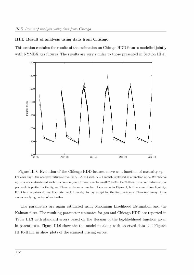
III.E. Result of analysis using data from Chicago
III.E Result of analysis using data from Chicago
This section contains the results of the estimation on Chicago HDD futures modelled jointly
with NYMEX gas futures. The results are very similar to those presented in Section III.4.
Jan−07 Apr−08 Jul−09 Oct−10 Jan−12200
400
600
800
1000
1200
1400
1600
Futu
res
pri
ces
Figure III.8. Evolution of the Chicago HDD futures curve as a function of maturity τ2.For each day t, the observed futures curve Ft(τ2−∆, τ2) with ∆ = 1 month is plotted as a function of τ2. We observe
up to seven maturities at each observation point t. From t = 1-Jan-2007 to 31-Dec-2010 one observed futures curve
per week is plotted in the figure. There is the same number of curves as in Figure 1, but because of low liquidity,
HDD futures prices do not fluctuate much from day to day except for the first contracts. Therefore, many of the
curves are lying on top of each other.
The parameters are again estimated using Maximum Likelihood Estimation and the
Kalman filter. The resulting parameter estimates for gas and Chicago HDD are reported in
Table III.3 with standard errors based on the Hessian of the log-likelihood function given
in parentheses. Figure III.9 show the the model fit along with observed data and Figures
III.10-III.11 in show plots of the squared pricing errors.
116
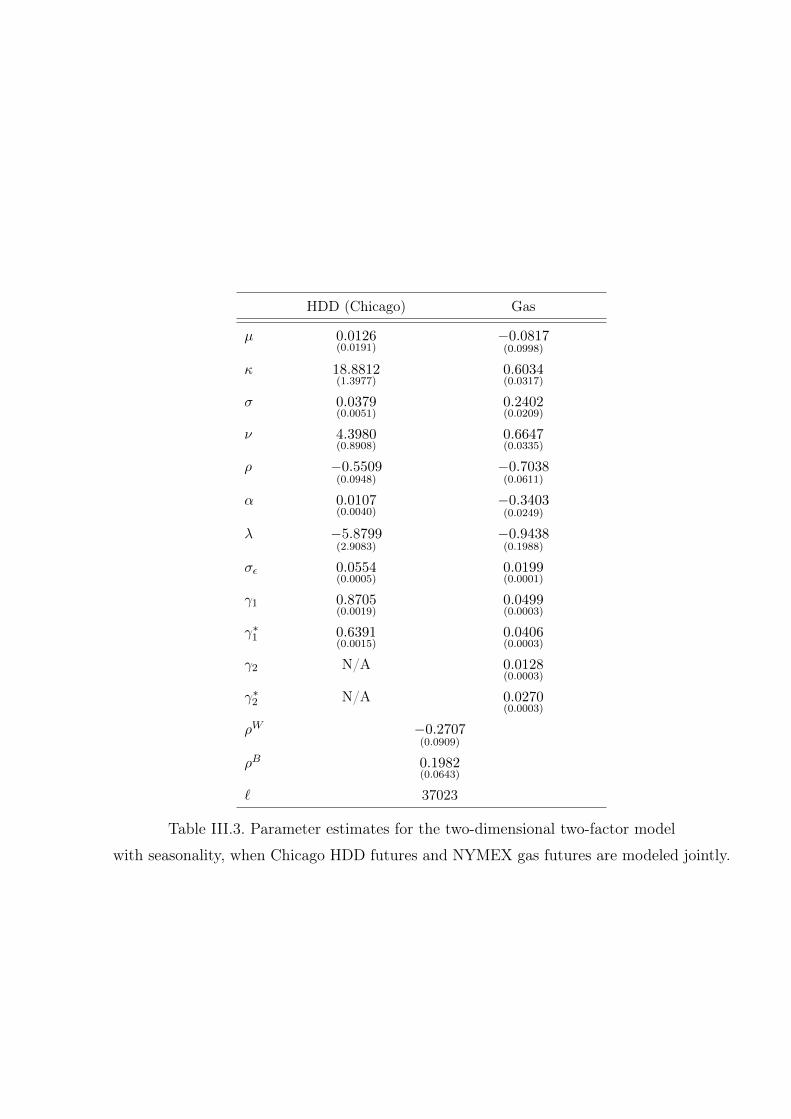
HDD (Chicago) Gas
µ 0.0126(0.0191)
−0.0817(0.0998)
κ 18.8812(1.3977)
0.6034(0.0317)
σ 0.0379(0.0051)
0.2402(0.0209)
ν 4.3980(0.8908)
0.6647(0.0335)
ρ −0.5509(0.0948)
−0.7038(0.0611)
α 0.0107(0.0040)
−0.3403(0.0249)
λ −5.8799(2.9083)
−0.9438(0.1988)
σε 0.0554(0.0005)
0.0199(0.0001)
γ1 0.8705(0.0019)
0.0499(0.0003)
γ∗1 0.6391(0.0015)
0.0406(0.0003)
γ2 N/A 0.0128(0.0003)
γ∗2 N/A 0.0270(0.0003)
ρW −0.2707(0.0909)
ρB 0.1982(0.0643)
` 37023
Table III.3. Parameter estimates for the two-dimensional two-factor model
with seasonality, when Chicago HDD futures and NYMEX gas futures are modeled jointly.
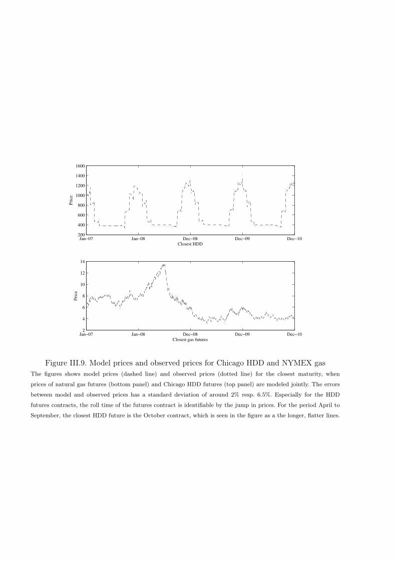
Jan−07 Jan−08 Dec−08 Dec−09 Dec−10200
400
600
800
1000
1200
1400
1600
Closest HDD
Pri
ce
Jan−07 Jan−08 Dec−08 Dec−09 Dec−102
4
6
8
10
12
14
Closest gas futures
Pri
ce
Figure III.9. Model prices and observed prices for Chicago HDD and NYMEX gasThe figures shows model prices (dashed line) and observed prices (dotted line) for the closest maturity, when
prices of natural gas futures (bottom panel) and Chicago HDD futures (top panel) are modeled jointly. The errors
between model and observed prices has a standard deviation of around 2% resp. 6.5%. Especially for the HDD
futures contracts, the roll time of the futures contract is identifiable by the jump in prices. For the period April to
September, the closest HDD future is the October contract, which is seen in the figure as a the longer, flatter lines.

Jan−07 Dec−08 Dec−100
0.05
closest
SE
Jan−07 Dec−08 Dec−100
0.01
0.02
2nd closest
SE
Jan−07 Dec−08 Dec−100
0.01
0.02
3rd closest
SE
Jan−07 Dec−08 Dec−100
0.01
0.02
4th closest
SE
Jan−07 Dec−08 Dec−100
0.01
0.02
5th closest
SE
Jan−07 Dec−08 Dec−100
0.01
0.02
6th closest
SE
Jan−07 Dec−08 Dec−100
0.005
0.01
7th closest
SE
Jan−07 Dec−08 Dec−100
0.005
0.01
8th closest
SE
Jan−07 Dec−08 Dec−100
0.005
0.01
9th closest
SE
Jan−07 Dec−08 Dec−100
0.005
0.01
10th closest
SE
Jan−07 Dec−08 Dec−100
0.005
0.01
11th closest
SE
Jan−07 Dec−08 Dec−100
0.01
0.02
12th closest
SE
Figure III.10. Time series of squared percentage pricing errors for gas.The figure shows the time series of squared pricing errors of the percentage difference between fitted and actual
NYMEX natural gas futures prices when modeled jointly with Chicago HDD futures. The pricing errors are largest
around the 2008 boom/bust in energy prices.
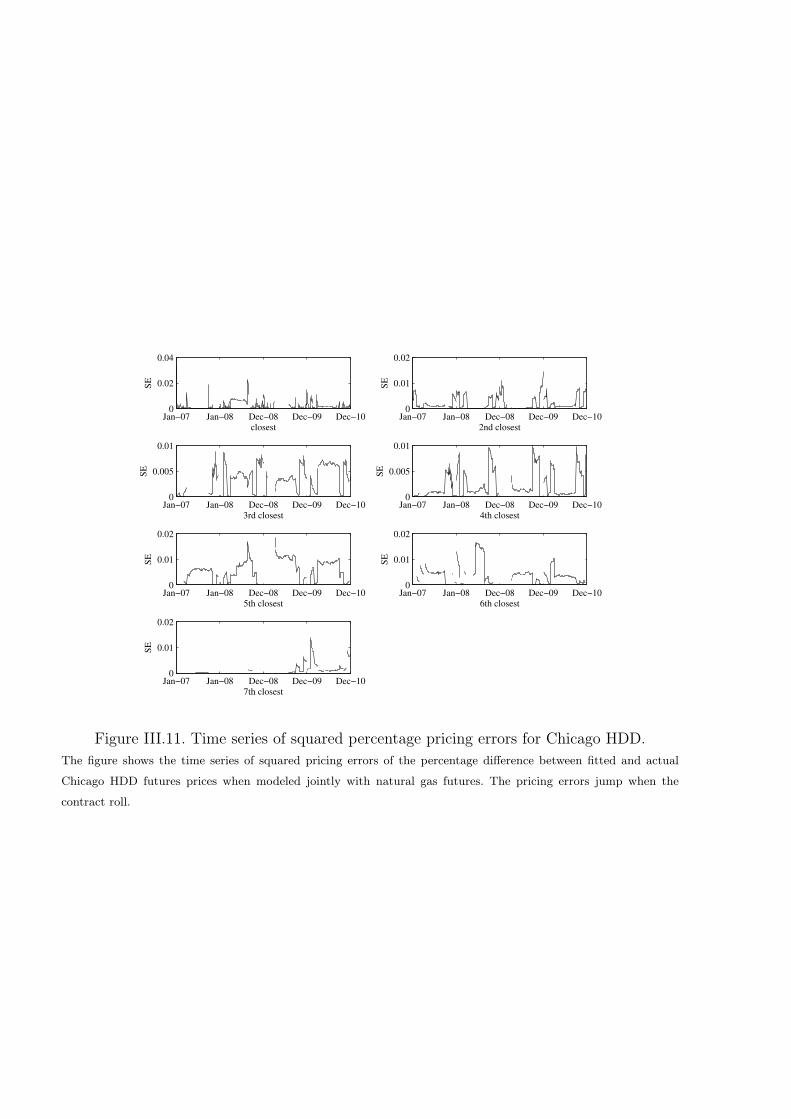
Jan−07 Jan−08 Dec−08 Dec−09 Dec−100
0.01
0.02
7th closest
SE
Jan−07 Jan−08 Dec−08 Dec−09 Dec−100
0.01
0.02
6th closest
SE
Jan−07 Jan−08 Dec−08 Dec−09 Dec−100
0.01
0.02
5th closest
SE
Jan−07 Jan−08 Dec−08 Dec−09 Dec−100
0.005
0.01
4th closest
SE
Jan−07 Jan−08 Dec−08 Dec−09 Dec−100
0.005
0.01
3rd closest
SE
Jan−07 Jan−08 Dec−08 Dec−09 Dec−100
0.01
0.02
2nd closest
SE
Jan−07 Jan−08 Dec−08 Dec−09 Dec−100
0.02
0.04
closest
SE
Figure III.11. Time series of squared percentage pricing errors for Chicago HDD.The figure shows the time series of squared pricing errors of the percentage difference between fitted and actual
Chicago HDD futures prices when modeled jointly with natural gas futures. The pricing errors jump when the
contract roll.
A Short Note on Pricing of Energy Quanto Options
Essay IV
A Short Note on Pricing of Energy Quanto Options
Abstract
In energy markets, market prices and demand are often positively
correlated leading to an amplified risk for e.g., retail energy companies.
Because of standardized derivatives’ inability to hedge this risk,
market participants have turned to using contracts that pay off
dependent on both energy prices and a load-correlated variable such as
a weather index. An example of such a contract is the so-called ”energy
quanto” option that only pays off, if both prices and the weather index
are high (or if both are low). Under the assumption of a log-normal
framework, the energy quanto option price can be approximated by
a pricing formula involving the correlation, current individual asset
prices and option prices, volatilities and Greeks. These quantities are
known or can be assessed by market participants, thereby yielding a
fast pricing method for energy quanto options.
121

IV.1. Introduction
IV.1 Introduction
A major risk in commodity markets is the quantity risk arising from the participants not
having full control over production or consumption. A classic example from the world of
energy is the Load Serving Entity, who needs to provide their electricity retail customers
with the demanded quantity at a pre-determined rate. As price and quantity is positively
correlated, this could lead to an undesired situation, when price and quantity are high as
this leads to a loss for the LSE, or when price and quantity are low as this leads to only a
small revenue. Also in agriculture, a farmer faces quantity risk as he is selling his crops at
market prices, while not being able to control the exact production.
In Essay II, it was argued why double structure options or energy quanto options as
discussed in Caporin et al. (2012) and Benth et al. (2015) is a natural contract structure
when hedging quantity risks. The applicability of these is further supported by statements
from re-insurance companies as Swiss Re1 and Munich Re2. The pricing question, also
addressed in e.g., Jørgensen (2007), Caporin et al. (2012) and Benth et al. (2015), is in
practice complicated, as the underlying contracts are often not traded liquidly in the market
and pricing methods would either rely on assumptions about risk-neutral distribution or an
actuarial approach, where the price is set according to an acceptable loss.
In this note, a price approximation formula is derived. Assuming a log-normal framework
for the two underlying assets, a price approximation is stated in terms of Deltas, Gammas,
single options, (integrated) volatility and correlation of underlying (log-)prices. Some of the
values are given in case of liquidly traded markets and otherwise a value that a market
participant has an opinion about. The log-normal framework encompasses models like
Schwartz and Smith (2000), Sørensen (2002) or the multi-factor model first introduced
by Clewlow and Strickland (1999) and further analysed in Benth and Koekebakker (2008).
The approximation formula is presented in the next section and a numerical example
illustrates the pricing error and behaviour. All proofs are given in Appendix IV.A and IV.B.
IV.2 The Quick and Dirty Formulas
Assume that the energy quanto option is written on two underlying assets that follows a
joint log-normal distributed. More specifically, the future energy price can be written as
1http://www.swissre.com/corporate_solutions/weather_risk_solutions_double_trigger.html2Munich Re: Topics Risk solutions, Issue 4, 2014
122
A Short Note on Pricing of Energy Quanto Options
ET = E0eµE+σEX and the future index contract’s price can be written as IT = I0e
µI+σIY ,
where (X,Y ) is standard bivariate normal with correlation ρ. The price of an energy quanto
option with strikes KE resp. KI is then given as
C(E0, I0; ρ) =e−rTEQ[max
(E0e
muE+σEX −KE, 0)×max
(I0e
µI+σIY −KI , 0)]
(IV.1)
To approximate the price of the energy quanto option, a first order Taylor approximation
of (IV.1) around ρ = 0 gives the following approximation for the energy quanto prices3:
Proposition IV.1 (First order approximation for energy quanto option)
Using the above introduced notation; when the underlying asset are log-normally distributed
under the pricing measure, the energy quanto option price can be approximated using
individual option prices, current asset values, Deltas, volatilities and correlation of log-
prices:
C(E0, I0; ρ) ≈C(E0, I0; 0) + ρ∂C
∂ρ(E0, I0; 0)
=erT [CE(E0)CI(I0) + ρE0I0σEσI∆E∆I ] (IV.2)
Here, CE(E0) denote the price and ∆E the option ∆ for a corresponding call option on
energy with strike KE and similar for the index4. 2
Proof: This results is derived from a first order Taylor approximation of (IV.1) around
ρ = 0. See the details in appendix IV.A.
Proposition IV.2 (Second order approximation for energy quanto option)
When the underlying asset are log-normally distributed under the pricing measure, the
energy quanto option price can be approximated using individual option prices, current
asset prices, Deltas and Gammas, volatilities and correlation of log-prices:
C(E0, I0; ρ) ≈C(E0, I0; 0) + ρ∂C
∂ρ(E0, I0; 0) + 1
2
∂2C
∂ρ2(E0, I0; 0)
=erT[CE(E0)CI(I0) + ρE0I0σEσI∆E∆I
+ 12ρ2E0I0σ
2Eσ
2I [ΓE∆IE0 + ∆E∆I + ΓEΓIE0I0 + ΓI∆EI0]
](IV.3)
3Similar price approximations can be derived for a product of swaps (the so-called energy quanto swaps), but not
for spread options as the derivative with respect to ρ is not multiplicative.4σi denotes the square root of the integrated variance of the contract from today to maturity. In the most simple
case such as Black-Scholes, this equals σ√T
123
IV.3. Numerical Example
Proof: This results is derived from a second order Taylor approximation of (IV.1) around
ρ = 0. See the details in appendix IV.A.
As an energy quanto option price has to be non-negative, the price approximations should
further be capped at zero.
IV.3 Numerical Example
The proposed formula enables us to write the price of an energy quanto option in terms of
individual option prices, deltas and volatilities. Obviously, the approximation will be best
around ρ = 0. Figures IV.1-IV.2 show the performance of IV.1 and IV.2 for the values given
in Table IV.1.
E0 KE σE I0 KI σI r T
4 4 0.4 1000 1000 0.5 0 1
Table IV.1. Parameters for numerical example.
Figure IV.1 shows the exact energy quanto option price for the parameters given in
Table IV.1 as well as the two price approximations. The energy quanto option price
is convex in correlation, so with the price approximation in Proposition IV.1 being
linear, the approximation will always underestimate the true price. Further, it will at
not be a relevant approximation once the correlation becomes sufficiently negative after
which the approximation returns a negative value. The approximation in Proposition
IV.2 underestimates the price as correlation increases and overestimates the price when
correlation decreases.
Figure IV.2 show the percentage price error:
Error =Price− Approximation
Price
The first order price approximation quickly becomes large, when the correlation deviates
from zero. The second order price approximations is more accurate. For the parameters
given in Table IV.1, the absolute pricing error is less than 1%, when correlation is between
−0.4 and 0.4. The price approximations is less than 4% for positive correlations, but grows
to (minus) infinity as the true price converges to zero. The large pricing error for strong
124
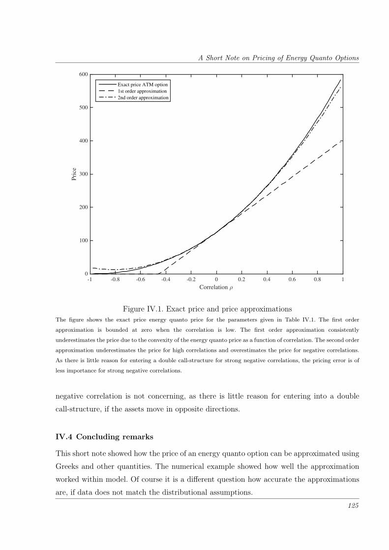
A Short Note on Pricing of Energy Quanto Options
Correlation ρ
-1 -0.8 -0.6 -0.4 -0.2 0 0.2 0.4 0.6 0.8 1
Pri
ce
0
100
200
300
400
500
600
Exact price ATM option
1st order approximation
2nd order approximation
Figure IV.1. Exact price and price approximationsThe figure shows the exact price energy quanto price for the parameters given in Table IV.1. The first order
approximation is bounded at zero when the correlation is low. The first order approximation consistently
underestimates the price due to the convexity of the energy quanto price as a function of correlation. The second order
approximation underestimates the price for high correlations and overestimates the price for negative correlations.
As there is little reason for entering a double call-structure for strong negative correlations, the pricing error is of
less importance for strong negative correlations.
negative correlation is not concerning, as there is little reason for entering into a double
call-structure, if the assets move in opposite directions.
IV.4 Concluding remarks
This short note showed how the price of an energy quanto option can be approximated using
Greeks and other quantities. The numerical example showed how well the approximation
worked within model. Of course it is a different question how accurate the approximations
are, if data does not match the distributional assumptions.
125
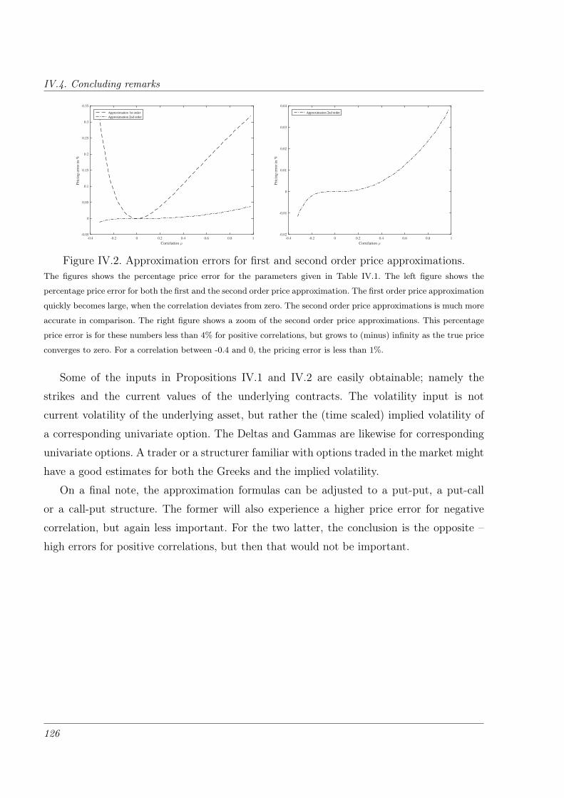
IV.4. Concluding remarks
Correlation ρ
-0.4 -0.2 0 0.2 0.4 0.6 0.8 1
Pri
cin
g e
rro
r in
%
-0.05
0
0.05
0.1
0.15
0.2
0.25
0.3
0.35
Approximation 1st order
Approximation 2nd order
Correlation ρ
-0.4 -0.2 0 0.2 0.4 0.6 0.8 1
Pri
cin
g e
rro
r in
%
-0.02
-0.01
0
0.01
0.02
0.03
0.04
Approximation 2nd order
Figure IV.2. Approximation errors for first and second order price approximations.The figures shows the percentage price error for the parameters given in Table IV.1. The left figure shows the
percentage price error for both the first and the second order price approximation. The first order price approximation
quickly becomes large, when the correlation deviates from zero. The second order price approximations is much more
accurate in comparison. The right figure shows a zoom of the second order price approximations. This percentage
price error is for these numbers less than 4% for positive correlations, but grows to (minus) infinity as the true price
converges to zero. For a correlation between -0.4 and 0, the pricing error is less than 1%.
Some of the inputs in Propositions IV.1 and IV.2 are easily obtainable; namely the
strikes and the current values of the underlying contracts. The volatility input is not
current volatility of the underlying asset, but rather the (time scaled) implied volatility of
a corresponding univariate option. The Deltas and Gammas are likewise for corresponding
univariate options. A trader or a structurer familiar with options traded in the market might
have a good estimates for both the Greeks and the implied volatility.
On a final note, the approximation formulas can be adjusted to a put-put, a put-call
or a call-put structure. The former will also experience a higher price error for negative
correlation, but again less important. For the two latter, the conclusion is the opposite –
high errors for positive correlations, but then that would not be important.
126
A Short Note on Pricing of Energy Quanto Options
Appendix
IV.A Proof of propositions IV.1-IV.2
Let Y = ρX +√
1− ρ2Z, where Z ∼ N (0, 1) and independent of X. Then (X, ρX +√1− ρ2Z) has the same distribution as (X,Y ). The derivative of the quanto option price
with respect to ρ and later evaluated at ρ = 0 is given by:
∂C
∂ρ(E0, I0; ρ) = EQ
[e−rT (E0e
µE+σEX −KE)+ × ∂
∂ρ
(I0e
µI+σI(ρX+√
1−ρ2Z) −KI
)+]
= e−rTEQ[(E0e
µE+σEX −KE
)+ × 1I0e
µI+σI(ρX+√
1−ρ2Z) > KI
× I0e
µI+σI(ρX+√
1−ρ2Z)σI
(X − ρ√
1− ρ2Z
)](IV.4)
∂C
∂ρ(E0, I0; 0) = e−rTEQ
[X(E0e
µE+σEX −KE
)+ × 1I0e
µI+σIZ > KI
× I0e
µI+σIZσI]
= e−rTEQ[X(E0e
µE+σEx −KE)+]EQ[1I0e
µI+σIZ > KI
eµI+σIZ
]I0σI
= erT∆E∆IE0I0σEσI
The latter equality follows by Lemmas IV.3 and IV.4.
To find the second derivative with respect to ρ, the first derivative as given in equation
(IV.4) is first expressed in terms of integrals and then differentiated. To ease the notation,
let dE = log(KE/E0)−µEσE
and dI(x, ρ) = log(KI/I0)−µIσI√
1−ρ2− ρ√
1−ρ2x:
erT∂C
∂ρ(E0, I0; ρ) =
∫ ∞dE
(E0e
µE+σEx −KE
)φ(x)I0σI[∫ ∞
dI(x,ρ)
eµI+σI
(ρx+√
1−ρ2z)(
x− ρ√1− ρ2
z
)φ(z)dz
]dx
erT∂2C
∂ρ2(E0, I0; ρ) =
∫ ∞dE
(E0e
µE+σEx −KE
)φ(x)I0σI (IV.5)
∂
∂ρ
[∫ ∞dI(x,ρ)
eµI+σI
(ρx+√
1−ρ2z)(
x− ρ√1− ρ2
z
)φ(z)dz
]dx
127
IV.B. Delta and Gamma expressions
Set f(z, ρ) = eµI+σI
(ρx+√
1−ρ2z)(
x− ρ√1−ρ2
z
)φ(z). Then ∂
∂ρ[· · · ] in the equation above is
given by
∂
∂ρ
[∫ ∞dI(x,ρ)
f(z, ρ)dz
]=
∫ ∞dI(x,ρ)
∂
∂ρf(z, ρ)dz − f(dI(x, ρ), ρ)
∂
∂ρdI(x, ρ)
= −∫ ∞dI(x,ρ)
eµI+σI
(ρx+√
1−ρ2z)
z
(1− ρ2)3/2φ(z)dz
+
∫ ∞dI(x,ρ)
σIeµI+σI
(ρx+√
1−ρ2z)(
x− ρ√1− ρ2
z
)2
φ(z)dz
− KI
I0
(x− ρ
1− ρ2
(log(KI/I0)−µI
σI− ρx
))φ(dI(x, ρ))
×(
log(KI/I0)−µIσI
ρ− x) 1
(1− ρ2)3/2
Evaluating this in ρ = 0 yields (with dI(x, 0) = dI):∫ ∞dI
σIeµI+σIzx2φ(z)dz −
∫ ∞dI
eµI+σIzzφ(z)dz +KI
I0
x2φ (dI)
Inserting in (IV.5):
erT∂2C
∂ρ2(E0, I0; 0) = I0σI
∫ ∞dE
x2(E0e
µE+σEx −KE
)φ(x)dx
∫ ∞dI
σIeµI+σIzφ(z)dz
+ I0σI
∫ ∞dE
x2(E0e
µE+σEx −KE
)φ(x)dx
KI
I0
φ (dI)
− I0σI
∫ ∞dE
(E0e
µE+σEx −KE
)φ(x)dx
∫ ∞dI
eµI+σIzzφ(z)dz
= I0σ2IEQ
[max(E0e
µE+σEX −KE, 0)X2]EQ[1I0e
µI+σIZ > KI
eµI+σIZ
]+ σIEQ
[max(E0e
µE+σEX −KE, 0)X2]KIφ (dI)
− I0σIEQ[max(E0e
µE+σEX −KE, 0)]EQ[1I0e
µI+σIZ > KI
eµI+σIZZ
]= e2rT I0E0σ
2Iσ
2E(E0ΓE∆I + ∆E∆I + I0E0ΓIΓE + I0ΓI∆E)
which with the help of Lemmas IV.4-IV.7 gives Proposition IV.2.
IV.B Delta and Gamma expressions
Assume that the asset price is log-normally distributed under the pricing measure Q;
ET = E0eµ+σX . If it is a futures contract, then µ = −1
2σ2. If it is a stock µ = rT − 1
2σ2. In
128
A Short Note on Pricing of Energy Quanto Options
the following interest rates are held constant. Without loss of generality, it is assumed that
today is time 0.
Lemma IV.3 (Delta expression 1) Assume ET = E0eµ+σX . Then
∆ =∂
∂E0
EQ[e−rT (ET −K)+
]=e−rT
E0σEQ[X(E0e
µ+σX −K)+]
Proof: The expression is shown by first doing integration by substitution and then changing
the order of differentiation and integration:
∆ =∂
∂E0
EQ[e−rT (ET −K)+
]=e−rT√
2π
∂
∂E0
∫R
(E0e
µ+σx −K)+e−
12x2
dx
=e−rT√2πσ
∂
∂E0
∫R
(eµ+t −K
)+e−
12σ2 (t−logE0)2
dt
=e−rT√2πσ
∫R
(eµ+t −K
)+e−
12σ2 (t−logE0)2 1
E0σ2(t− logE0)dt
=e−rT√
2π
∫R
(E0e
µ+σx −K)+e−
12x2 1
E0σxdx
=e−rT
E0σEQ[X(E0e
µ+σX −K)+]
Lemma IV.4 (Delta expression 2) Assume ET = E0eµ+σX . Then
∆ =∂
∂E0
EQ[e−rT (ET −K)+
]= e−rTEQ
[1E0e
µ+σX > Keµ+σX
]Proof: The expression is shown by changing the order of differentiation and integration
∆ =∂
∂E0
EQ[e−rT (ET −K)+
]=
∂
∂E0
∫ ∞−∞
e−rT (E0eµ+σx −K)+φ(x)dx
= e−rT∫ ∞−∞
∂
∂E0
(E0eµ+σx −K)+φ(x)dx
= e−rT∫ ∞−∞
[1E0e
µ+σx > Keµ+σx
]φ(x)dx
= e−rTEQ[1E0e
µ+σX > Keµ+σX
]Note, that the normality assumption was not needed for this Delta-expression.
129

IV.B. Delta and Gamma expressions
Lemma IV.5 (Gamma expression 1) Assume ET = E0eµ+σX . Then
Γ =∂∆
∂E0
=e−rT
σE0
EQ[1E0e
µ+σX > Keµ+σXX
]− ∆
E0
Proof: This expression is derived by differentiating the ∆-expression in Lemma IV.3:
Γ =∂
∂E0
e−rT
E0σEQ[X(E0e
µ+σX −K)+]
=e−rT
E0σ
∂
∂E0
(EQ[X(E0e
µ+σX −K)+])
+∂
∂E0
(e−rT
E0σ
)EQ[X(E0e
µ+σX −K)+]
=e−rT
E0σ
∂
∂E0
∫ ∞log(K/E0)−µ
σ
x(E0e
µ+σx −K)φ(x)dx− ∆
E0
=e−rT
E0σEQ[Xeµ+σX1
E0e
µ+σX > K]− ∆
E0
Lemma IV.6 (Gamma expression 2) Assume ET = E0eµ+σX . Then
Γ =∂∆
∂E0
=e−rT
σE0
K
E0
φ
(log (E0/K) + µ
σ
)Proof: This expression is derived by differentiating the ∆-expression in Lemma IV.4:
Γ =∂
∂E0
e−rTEQ[1E0e
µ+σX > Keµ+σX
]= e−rT
∂
∂E0
∫ ∞log(K/E0)−µ
σ
eµ+σxφ(x)dx
= e−rT∂
∂E0
log(K/E0)− µσ
eµ+σlog(K/E0)−µ
σ φ(
log(K/E0)−µσ
)=e−rT
σE0
K
E0
φ(
log(K/E0)−µσ
)
Lemma IV.7 (Gamma expression 3) Assume ET = E0eµ+σX . Then
Γ =∂∆
∂E0
=e−rT
σ2E20
EQ[max(E0e
µ+σX −K, 0)X2]− C
σ2E20
− ∆
E0
130
A Short Note on Pricing of Energy Quanto Options
Proof: This expression is derived by differentiating the ∆-expression in Lemma IV.3 and
doing integration by substition:
Γ =e−rT
E0σ
∂
∂E0
(EQ[X(E0e
µ+σX −K)+])− ∆
E0
=e−rT
E0σ√
2π
∂
∂E0
∫Rx(E0e
µ+σx −K)+e−
12x2
dx− ∆
E0
=e−rT
E0σ2√
2π
∂
∂E0
∫R
t− logE0
σ
(eµ+t −K
)+e−
12σ2 (t−logE0)2
dt− ∆
E0
=e−rT
E0σ2√
2π
∫R
t− logE0
σ
(eµ+t −K
)+ ∂
∂E0
e−1
2σ2 (t−logE0)2
dt
+e−rT
E0σ2√
2π
∫R
∂
∂E0
t− logE0
σ
(eµ+t −K
)+e−
12σ2 (t−logE0)2
dt− ∆
E0
=e−rT
E20σ
2√
2π
∫Rx2(E0e
µ+σx −K)+e−
12x2
dx
+e−rT
E20σ
2√
2π
∫R
(E0e
µ+σx −K)+e−
12x2
dx− ∆
E0
=e−rT
σ2E20
EQ[max(E0e
µ+σX −K, 0)X2]− C
σ2E20
− ∆
E0
131


Conclusion
Conclusion
This dissertation presented four essays related to correlation in energy markets. How prices
relate is generally important for risk management and derivatives pricing purposes and the
understanding of these relationships and the risk arising from them is therefore interesting.
The first essay investigated if and how volatility of two different markets, the WTI
crude oil market and the EURUSD market, changed over time. The analysis is done using
market-perceived volatilities in the form of options and futures and shows a joint factor
after mid-2007. The conclusion was made based on both a model-free approach and the
estimation of a term structure model for futures and options on oil and futures and options
on EURUSD. The cause of this volatility-relation is a question left unanswered. A natural
extension of this essay would be to investigate the effect of fundamentals, financialization
and the latest financial crisis.
The second essay compares energy quanto options as a risk management tool to other
approaches proposed in the literature and shows that that it performs well in a simple one-
period model. An energy quanto option has an easy and understandable structure and as
they are already offered in the market, their potential for risk management using real data
is a relevant next area to study, if it is possible to obtain load data from a Load Serving
Entity.
The third essay and fourth essay concentrates on pricing energy quanto options. If the
energy quanto option is written as an average over a period of time, it is possible to convert
the rewrite the problem in terms of options on futures covering the same period of time. In
a log-normal framework, closed form solutions are available both for prices and Greeks and
prices can further be approximated using the prices and Greeks of the univariate options
along with the correlation.
133

Bibliography
Bibliography
Aase, K. K. (2004). A Pricing Model for Quantity Contracts. The Journal of Risk and
Insurance 71 (4), 617–642.
Alexander, C. (1999). Correlation and Cointegration in Energy Markets. In Managing
Energy Price Risk, pp. 297–304. RISK Publications.
Amano, R. A. and S. van Norden (1998). Exchange Rates and Oil Prices. Review of
International Economics 6(4), 683–694.
Bakshi, G., P. Carr, and L. Wu (2008). Stochastic Risk Premiums, Stochastic Skewness in
Currency Options, and Stochastic Discount Factors in International Economies.
Journal of Financial Economics 87 (1), 132–156.
Barone-Adesi, G. and R. E. Whaley (1987). Efficient Analytical Approximation of
American Option Values. The Journal of Finance 42 (2), 301–320.
Basak, S. and A. Pavlova (2016). A Model of Financialization of Commodities. Journal of
Finance 71 (4), 1511–1556.
Bellini, F. (2005). The weather derivatives market: Modeling and pricing temperature. Ph.
D. thesis, University of Lugano.
Benth, F. E. and J. Š. Benth (2013). Modeling and Pricing in Financial Markets for
Weather Derivatives. World Scientific.
Benth, F. E., J. Š. Benth, and S. Koekebakker (2008). Stochastic Modelling of Electricity
and Related Markets. World Scientific.
Benth, F. E. and S. Koekebakker (2008). Stochastic Modeling of Financial Electricity
Contracts. Energy Economics 30 (3), 1116–1157.
Benth, F. E., N. Lange, and T. Å. Myklebust (2015). Pricing and Hedging Quanto
Options in Energy Markets. Journal of Energy Markets 8 (1), 1–36.
135

Bibliography
Black, F. (1976). The pricing of commodity contracts. Journal of Financial
Economics 3 (1-2), 167–179.
Brown, G. W. and K. B. Toft (2002). How Firms Should Hedge. Review of Financial
Studies 15 (4), 1283–1324.
Caporin, M., J. Preś, and H. Torro (2012). Model based Monte Carlo pricing of energy
and temperature Quanto options. Energy Economics 34 (5), 1700–1712.
Carmona, R. (2015). Financialization of the commodities markets: A non-technical
introduction. Fields Institute Communications 74, 3–37.
Carr, P. and D. Madan (2001). Optimal positioning in derivative securities. Quantitative
Finance 1 (1), 19–37.
Chen, S.-S. and H.-C. Chen (2007). Oil prices and real exchange rates. Energy
Economics 29 (3), 390–404.
Chen, Y.-C., K. Rogoff, and B. Rossi (2010). Can exchange rates forecast commodity
prices? The Quarterly Journal of Economics , 1145–1194.
Chiarella, C., B. Kang, C. S. Nikitopoulos, and T.-D. Tô (2013). Humps in the volatility
structure of the crude oil futures market: New evidence. Energy Economics 40,
989–1000.
Christoffersen, P., A. Lunde, and K. V. Olesen (2014). Factor Structure in Commodity
Futures Return and Volatility Factor Structure in Commodity Futures Return and
Volatility. CREATES research paper, Aarhus University 31 .
Clewlow, L. and C. Strickland (1999). A Multi-Factor Model for Energy Derivatives.
QFRC Research Paper Series, University of Technology, Sydney .
Clewlow, L. and C. Strickland (2000). Energy Derivatives: Pricing and Risk Management.
Lacima Publications.
Considine, G. (2000). Introduction to Weather Derivatives. Technical report, CME Group.
Cornaggia, J. (2013). Does risk management matter? Evidence from the U.S. agricultural
industry. Journal of Financial Economics 109 (2), 419–440.
Cortazar, G., S. Gutierrez, and H. Ortega (2016). Empirical Performance of Commodity
Pricing Models: When is it Worthwhile to Use a Stochastic Volatility Specification?
Journal of Futures Markets 36 (5), 457–487.
136

Bibliography
Cortazar, G. and L. Naranjo (2006). An N-factor Gaussian model of oil futures prices.
Journal of Futures Markets 26 (3), 209–313.
Cucu, L., R. Döttling, P. Heider, and S. Maina (2016). Managing temperature-driven
volume risks. Journal of Energy Markets 9 (2), 95–110.
Davis, A. (2010). A new direction for weather derivatives.
http://www.risk.net/energy-risk/feature/1652654/a-direction-weather-derivatives .
Diebold, F. and R. Mariano (1995). Comparing Predictive Accuracy. Journal of Business
and Economic Statistics 13, 252–263.
Ding, L. and M. Vo (2012). Exchange rates and oil prices: A multivariate stochastic
volatility analysis. Quarterly Review of Economics and Finance 52 (1), 15–37.
Engle, R. F., C. Mustafa, and J. Rice (1992). Modelling peak electricity demand. Journal
of Forecasting 11 (3), 241–251.
Eydeland, A. and K. Wolyniec (2003). Energy and Power Risk Management. John Wiley
& Sons.
Fratzscher, M., D. Schneider, and I. V. Robays (2014). Oil Prices, Exchange Rates and
Asset Prices. ECB Working Paper Series (1689), 1–43.
Galeano, P. and D. Wied (2014). Multiple break detection in the correlation structure of
random variables. Computational Statistics and Data Analysis 76, 262–282.
Garman, M. B. and S. W. Kohlhagen (1983). Foreign currency option values. Journal of
International Money and Finance 2 (3), 231–237.
Geman, H. (2005). Commodities and commodity derivatives. John Wiley & Sons.
Geman, H. (2015). Agricultural Finance. John Wiley & Sons.
Golden, L. L., M. Wang, and C. Yang (2007). Handling weather related risks through the
financial markets: Considerations of credit risk, basis risk, and hedging. Journal of Risk
and Insurance 74 (2), 319–346.
Harvey, A. C. (1989). State space models and the Kalman filter. Cambridge University
Press.
Id Brik, R. and A. Roncoroni (2016a). Hedging Size Risk: Theory and Application to the
US Gas Market. http://papers.ssrn.com/sol3/papers.cfm?abstract_id=2790350 .
137
Bibliography
Id Brik, R. and A. Roncoroni (2016b). Static Mitigation of Volumetric Risk. Journal of
Energy Markets 9 (2), 111–150.
Jørgensen, P. L. (2007). Traffic light options. Journal of Banking & Finance 31 (12),
3698–3719.
Karatzas, I. and S. E. Shreve (2000). Brownian Motion and Stochastic Calculus. Springer.
Kilian, L. (2009). Not All Oil Price Shocks Are Alike: Disentangling Demand and Supply
Shocks in the Crude Oil Market. The American Economic Review 99 (3), 1053–1069.
Kleindorfer, P. R. P. R. and L. Li (2005). Multi-period VaR-constrained portfolio
optimization with applications to the electric power sector. The Energy Journal 26 (1),
1–26.
Korn, O. (2009). How firms should hedge: An Extension. Journal of Futures
Markets 30 (9), 834–845.
Lee, Y. and S. S. Oren (2009). An equilibrium pricing model for weather derivatives in a
multi-commodity setting. Energy Economics 31 (5), 702–713.
Lien, D. and D. A. Hennessy (2004). A note on price futures versus revenue futures
contracts. Journal of Futures Markets 24 (2), 503–512.
Lizardo, R. A. and A. V. Mollick (2010). Oil price fluctuations and U.S. dollar exchange
rates. Energy Economics 32 (2), 399–408.
Lucia, J. J. and E. S. Schwartz (2002). Electricity Prices and Power Derivatives: Evidence
from the Nordic Power Exchange. Review of Derivatives Research 5, 5–50.
Miltersen, K. R. and E. S. Schwartz (1998). Pricing of Options on Commodity Futures
with Stochastic Term Structure of Convenience Yields and Interest Rates. Journal of
Financial and Quantitative Analysis 33(1), 33–59.
Moschini, G. and H. Lapan (1995). The hedging role of options and futures under joint
price, basis and production risk. International Economic Review 36 (4), 1025–1049.
Munich Re (2014). Topics Risk solutions, Insurance solutions for industry, Issue 4/2014.
https://www.munichre.com/ .
Myers, R. (2008). What every CFO needs to know about weather risk management.
Technical report, CME Group.
138

Bibliography
Näsäkkälä, E. and J. Keppo (2005). Electricity load pattern hedging with static forward
strategies. Managerial Finance 31 (6), 116–137.
Oum, Y. and S. Oren (2006). Hedging quantity risks with standard power options in a
competitive wholesale electricity market. Naval Research Logistics 53 (7), 1–33.
Oum, Y. and S. Oren (2010). Optimal Static Hedging of Volumetric Risk in a Competitive
Wholesale Electricity Market. Decision Analysis 7 (1), 107–122.
Pérez-González, F. and H. Yun (2013). Risk management and firm value: Evidence from
weather derivatives. The Journal of Finance 68 (5), 2143–2176.
Pilz, K. F. and E. Schlögl (2012). A Hybrid Commodity and Interest Rate Market Model.
Quantitative Finance 13 (1), 1–18.
Poitras, G. (2013). Commodity Risk Management. Routledge.
Schwartz, E. S. (1997). The Stochastic Behavior of Commodity Prices: Implications for
Valuation and Hedging. The Journal of Finance 52 (3), 923–973.
Schwartz, E. S. and J. E. Smith (2000). Short-term variations and long-term dynamics in
commodity prices: Implications for valuation and hedging. Management Science 46,
893–911.
Sørensen, C. (2002). Seasonality in Agricultural Commodity Futures. The Journal of
Futures Markets 22 (5), 393–426.
Swindle, G. (2014). Valuation and Risk Management in Energy Markets. Cambridge
University Press.
Tang, K. and W. Xiong (2012). Index investment and financialization of commodities.
Financial Analysts Journal 68 (6), 54–74.
Timmer, R. P. and P. J. Lamb (2007). Relations between temperature and residential
natural gas consumption in the Central and Eastern United States. Journal of Applied
Meteorology and Climatology 46 (11), 1993–2013.
Trolle, A. B. and E. S. Schwartz (2009). Unspanned Stochastic Volatility and the Pricing
of Commodity Derivatives. Review of Financial Studies 22 (11), 4423–4461.
Vansteenkiste, I. (2011). What is driving oil futures prices? Fundamentals versus
speculation. European Central Bank Working Paper .
Verleger, P. K. (2008). The Oil-Dollar Link. The International Economy , 46–50.
139

Bibliography
Wied, D., W. Krämer, and H. Dehling (2009). Testing for a Change in Correlation At an
Unknown Point in Time Using an Extended Functional Delta Method. Econometric
Theory 28 (3), 570–589.
Zhang, P. G. (1995). Correlation Digital Options. Journal of Financial Engineering 4 (1),
75–96.
140

TITLER I PH.D.SERIEN:
20041. Martin Grieger Internet-based Electronic Marketplaces and Supply Chain Management
2. Thomas Basbøll LIKENESS A Philosophical Investigation
3. Morten Knudsen Beslutningens vaklen En systemteoretisk analyse of mo-
derniseringen af et amtskommunalt sundhedsvæsen 1980-2000
4. Lars Bo Jeppesen Organizing Consumer Innovation A product development strategy that
is based on online communities and allows some firms to benefit from a distributed process of innovation by consumers
5. Barbara Dragsted SEGMENTATION IN TRANSLATION
AND TRANSLATION MEMORY SYSTEMS An empirical investigation of cognitive segmentation and effects of integra-
ting a TM system into the translation process
6. Jeanet Hardis Sociale partnerskaber Et socialkonstruktivistisk casestudie af partnerskabsaktørers virkeligheds-
opfattelse mellem identitet og legitimitet
7. Henriette Hallberg Thygesen System Dynamics in Action
8. Carsten Mejer Plath Strategisk Økonomistyring
9. Annemette Kjærgaard Knowledge Management as Internal Corporate Venturing
– a Field Study of the Rise and Fall of a Bottom-Up Process
10. Knut Arne Hovdal De profesjonelle i endring Norsk ph.d., ej til salg gennem Samfundslitteratur
11. Søren Jeppesen Environmental Practices and Greening Strategies in Small Manufacturing Enterprises in South Africa – A Critical Realist Approach
12. Lars Frode Frederiksen Industriel forskningsledelse – på sporet af mønstre og samarbejde
i danske forskningsintensive virksom-heder
13. Martin Jes Iversen The Governance of GN Great Nordic – in an age of strategic and structural transitions 1939-1988
14. Lars Pynt Andersen The Rhetorical Strategies of Danish TV Advertising A study of the first fifteen years with special emphasis on genre and irony
15. Jakob Rasmussen Business Perspectives on E-learning
16. Sof Thrane The Social and Economic Dynamics of Networks – a Weberian Analysis of Three Formalised Horizontal Networks
17. Lene Nielsen Engaging Personas and Narrative Scenarios – a study on how a user- centered approach influenced the perception of the design process in
the e-business group at AstraZeneca
18. S.J Valstad Organisationsidentitet Norsk ph.d., ej til salg gennem Samfundslitteratur
19. Thomas Lyse Hansen Six Essays on Pricing and Weather risk
in Energy Markets
20. Sabine Madsen Emerging Methods – An Interpretive Study of ISD Methods in Practice
21. Evis Sinani The Impact of Foreign Direct Inve-
stment on Efficiency, Productivity Growth and Trade: An Empirical Inve-stigation
22. Bent Meier Sørensen Making Events Work Or, How to Multiply Your Crisis
23. Pernille Schnoor Brand Ethos Om troværdige brand- og virksomhedsidentiteter i et retorisk og
diskursteoretisk perspektiv
24. Sidsel Fabech Von welchem Österreich ist hier die
Rede? Diskursive forhandlinger og magt-
kampe mellem rivaliserende nationale identitetskonstruktioner i østrigske pressediskurser
25. Klavs Odgaard Christensen Sprogpolitik og identitetsdannelse i flersprogede forbundsstater Et komparativt studie af Schweiz og Canada
26. Dana B. Minbaeva Human Resource Practices and Knowledge Transfer in Multinational Corporations
27. Holger Højlund Markedets politiske fornuft Et studie af velfærdens organisering i perioden 1990-2003
28. Christine Mølgaard Frandsen A.s erfaring Om mellemværendets praktik i en
transformation af mennesket og subjektiviteten
29. Sine Nørholm Just The Constitution of Meaning – A Meaningful Constitution? Legitimacy, identity, and public opinion
in the debate on the future of Europe
20051. Claus J. Varnes Managing product innovation through rules – The role of formal and structu-
red methods in product development
2. Helle Hedegaard Hein Mellem konflikt og konsensus – Dialogudvikling på hospitalsklinikker
3. Axel Rosenø Customer Value Driven Product Inno-
vation – A Study of Market Learning in New Product Development
4. Søren Buhl Pedersen Making space An outline of place branding
5. Camilla Funck Ellehave Differences that Matter An analysis of practices of gender and organizing in contemporary work-
places
6. Rigmor Madeleine Lond Styring af kommunale forvaltninger
7. Mette Aagaard Andreassen Supply Chain versus Supply Chain Benchmarking as a Means to Managing Supply Chains
8. Caroline Aggestam-Pontoppidan From an idea to a standard The UN and the global governance of accountants’ competence
9. Norsk ph.d.
10. Vivienne Heng Ker-ni An Experimental Field Study on the
Effectiveness of Grocer Media Advertising Measuring Ad Recall and Recognition, Purchase Intentions and Short-Term
Sales
11. Allan Mortensen Essays on the Pricing of Corporate
Bonds and Credit Derivatives
12. Remo Stefano Chiari Figure che fanno conoscere Itinerario sull’idea del valore cognitivo
e espressivo della metafora e di altri tropi da Aristotele e da Vico fino al cognitivismo contemporaneo
13. Anders McIlquham-Schmidt Strategic Planning and Corporate Performance An integrative research review and a meta-analysis of the strategic planning and corporate performance literature from 1956 to 2003
14. Jens Geersbro The TDF – PMI Case Making Sense of the Dynamics of Business Relationships and Networks
15 Mette Andersen Corporate Social Responsibility in Global Supply Chains Understanding the uniqueness of firm behaviour
16. Eva Boxenbaum Institutional Genesis: Micro – Dynamic Foundations of Institutional Change
17. Peter Lund-Thomsen Capacity Development, Environmental Justice NGOs, and Governance: The
Case of South Africa
18. Signe Jarlov Konstruktioner af offentlig ledelse
19. Lars Stæhr Jensen Vocabulary Knowledge and Listening Comprehension in English as a Foreign Language
An empirical study employing data elicited from Danish EFL learners
20. Christian Nielsen Essays on Business Reporting Production and consumption of
strategic information in the market for information
21. Marianne Thejls Fischer Egos and Ethics of Management Consultants
22. Annie Bekke Kjær Performance management i Proces- innovation – belyst i et social-konstruktivistisk perspektiv
23. Suzanne Dee Pedersen GENTAGELSENS METAMORFOSE Om organisering af den kreative gøren
i den kunstneriske arbejdspraksis
24. Benedikte Dorte Rosenbrink Revenue Management Økonomiske, konkurrencemæssige & organisatoriske konsekvenser
25. Thomas Riise Johansen Written Accounts and Verbal Accounts The Danish Case of Accounting and Accountability to Employees
26. Ann Fogelgren-Pedersen The Mobile Internet: Pioneering Users’ Adoption Decisions
27. Birgitte Rasmussen Ledelse i fællesskab – de tillidsvalgtes fornyende rolle
28. Gitte Thit Nielsen Remerger – skabende ledelseskræfter i fusion og opkøb
29. Carmine Gioia A MICROECONOMETRIC ANALYSIS OF MERGERS AND ACQUISITIONS

30. Ole Hinz Den effektive forandringsleder: pilot, pædagog eller politiker? Et studie i arbejdslederes meningstil-
skrivninger i forbindelse med vellykket gennemførelse af ledelsesinitierede forandringsprojekter
31. Kjell-Åge Gotvassli Et praksisbasert perspektiv på dynami-
ske læringsnettverk i toppidretten Norsk ph.d., ej til salg gennem Samfundslitteratur
32. Henriette Langstrup Nielsen Linking Healthcare An inquiry into the changing perfor- mances of web-based technology for asthma monitoring
33. Karin Tweddell Levinsen Virtuel Uddannelsespraksis Master i IKT og Læring – et casestudie
i hvordan proaktiv proceshåndtering kan forbedre praksis i virtuelle lærings-miljøer
34. Anika Liversage Finding a Path Labour Market Life Stories of Immigrant Professionals
35. Kasper Elmquist Jørgensen Studier i samspillet mellem stat og
erhvervsliv i Danmark under 1. verdenskrig
36. Finn Janning A DIFFERENT STORY Seduction, Conquest and Discovery
37. Patricia Ann Plackett Strategic Management of the Radical Innovation Process Leveraging Social Capital for Market Uncertainty Management
20061. Christian Vintergaard Early Phases of Corporate Venturing
2. Niels Rom-Poulsen Essays in Computational Finance
3. Tina Brandt Husman Organisational Capabilities, Competitive Advantage & Project-
Based Organisations The Case of Advertising and Creative Good Production
4. Mette Rosenkrands Johansen Practice at the top – how top managers mobilise and use non-financial performance measures
5. Eva Parum Corporate governance som strategisk kommunikations- og ledelsesværktøj
6. Susan Aagaard Petersen Culture’s Influence on Performance Management: The Case of a Danish Company in China
7. Thomas Nicolai Pedersen The Discursive Constitution of Organi-
zational Governance – Between unity and differentiation
The Case of the governance of environmental risks by World Bank
environmental staff
8. Cynthia Selin Volatile Visions: Transactons in Anticipatory Knowledge
9. Jesper Banghøj Financial Accounting Information and
Compensation in Danish Companies
10. Mikkel Lucas Overby Strategic Alliances in Emerging High-
Tech Markets: What’s the Difference and does it Matter?
11. Tine Aage External Information Acquisition of Industrial Districts and the Impact of Different Knowledge Creation Dimen-
sions
A case study of the Fashion and Design Branch of the Industrial District of Montebelluna, NE Italy
12. Mikkel Flyverbom Making the Global Information Society Governable On the Governmentality of Multi-
Stakeholder Networks
13. Anette Grønning Personen bag Tilstedevær i e-mail som inter-
aktionsform mellem kunde og med-arbejder i dansk forsikringskontekst
14. Jørn Helder One Company – One Language? The NN-case
15. Lars Bjerregaard Mikkelsen Differing perceptions of customer
value Development and application of a tool
for mapping perceptions of customer value at both ends of customer-suppli-er dyads in industrial markets
16. Lise Granerud Exploring Learning Technological learning within small manufacturers in South Africa
17. Esben Rahbek Pedersen Between Hopes and Realities: Reflections on the Promises and Practices of Corporate Social Responsibility (CSR)
18. Ramona Samson The Cultural Integration Model and European Transformation. The Case of Romania
20071. Jakob Vestergaard Discipline in The Global Economy Panopticism and the Post-Washington Consensus
2. Heidi Lund Hansen Spaces for learning and working A qualitative study of change of work, management, vehicles of power and social practices in open offices
3. Sudhanshu Rai Exploring the internal dynamics of
software development teams during user analysis
A tension enabled Institutionalization Model; ”Where process becomes the objective”
4. Norsk ph.d. Ej til salg gennem Samfundslitteratur
5. Serden Ozcan EXPLORING HETEROGENEITY IN ORGANIZATIONAL ACTIONS AND OUTCOMES A Behavioural Perspective
6. Kim Sundtoft Hald Inter-organizational Performance Measurement and Management in
Action – An Ethnography on the Construction
of Management, Identity and Relationships
7. Tobias Lindeberg Evaluative Technologies Quality and the Multiplicity of Performance
8. Merete Wedell-Wedellsborg Den globale soldat Identitetsdannelse og identitetsledelse
i multinationale militære organisatio-ner
9. Lars Frederiksen Open Innovation Business Models Innovation in firm-hosted online user communities and inter-firm project ventures in the music industry – A collection of essays
10. Jonas Gabrielsen Retorisk toposlære – fra statisk ’sted’
til persuasiv aktivitet
11. Christian Moldt-Jørgensen Fra meningsløs til meningsfuld
evaluering. Anvendelsen af studentertilfredsheds- målinger på de korte og mellemlange
videregående uddannelser set fra et psykodynamisk systemperspektiv
12. Ping Gao Extending the application of actor-network theory Cases of innovation in the tele- communications industry
13. Peter Mejlby Frihed og fængsel, en del af den
samme drøm? Et phronetisk baseret casestudie af frigørelsens og kontrollens sam-
eksistens i værdibaseret ledelse! 14. Kristina Birch Statistical Modelling in Marketing
15. Signe Poulsen Sense and sensibility: The language of emotional appeals in
insurance marketing
16. Anders Bjerre Trolle Essays on derivatives pricing and dyna-
mic asset allocation
17. Peter Feldhütter Empirical Studies of Bond and Credit
Markets
18. Jens Henrik Eggert Christensen Default and Recovery Risk Modeling
and Estimation
19. Maria Theresa Larsen Academic Enterprise: A New Mission
for Universities or a Contradiction in Terms?
Four papers on the long-term impli-cations of increasing industry involve-ment and commercialization in acade-mia
20. Morten Wellendorf Postimplementering af teknologi i den
offentlige forvaltning Analyser af en organisations konti-
nuerlige arbejde med informations-teknologi
21. Ekaterina Mhaanna Concept Relations for Terminological
Process Analysis
22. Stefan Ring Thorbjørnsen Forsvaret i forandring Et studie i officerers kapabiliteter un-
der påvirkning af omverdenens foran-dringspres mod øget styring og læring
23. Christa Breum Amhøj Det selvskabte medlemskab om ma-
nagementstaten, dens styringstekno-logier og indbyggere
24. Karoline Bromose Between Technological Turbulence and
Operational Stability – An empirical case study of corporate
venturing in TDC
25. Susanne Justesen Navigating the Paradoxes of Diversity
in Innovation Practice – A Longitudinal study of six very different innovation processes – in
practice
26. Luise Noring Henler Conceptualising successful supply
chain partnerships – Viewing supply chain partnerships
from an organisational culture per-spective
27. Mark Mau Kampen om telefonen Det danske telefonvæsen under den
tyske besættelse 1940-45
28. Jakob Halskov The semiautomatic expansion of
existing terminological ontologies using knowledge patterns discovered
on the WWW – an implementation and evaluation
29. Gergana Koleva European Policy Instruments Beyond
Networks and Structure: The Innova-tive Medicines Initiative
30. Christian Geisler Asmussen Global Strategy and International Diversity: A Double-Edged Sword?
31. Christina Holm-Petersen Stolthed og fordom Kultur- og identitetsarbejde ved ska-
belsen af en ny sengeafdeling gennem fusion
32. Hans Peter Olsen Hybrid Governance of Standardized
States Causes and Contours of the Global
Regulation of Government Auditing
33. Lars Bøge Sørensen Risk Management in the Supply Chain
34. Peter Aagaard Det unikkes dynamikker De institutionelle mulighedsbetingel-
ser bag den individuelle udforskning i professionelt og frivilligt arbejde
35. Yun Mi Antorini Brand Community Innovation An Intrinsic Case Study of the Adult
Fans of LEGO Community
36. Joachim Lynggaard Boll Labor Related Corporate Social Perfor-
mance in Denmark Organizational and Institutional Per-
spectives
20081. Frederik Christian Vinten Essays on Private Equity
2. Jesper Clement Visual Influence of Packaging Design
on In-Store Buying Decisions
3. Marius Brostrøm Kousgaard Tid til kvalitetsmåling? – Studier af indrulleringsprocesser i
forbindelse med introduktionen af kliniske kvalitetsdatabaser i speciallæ-gepraksissektoren
4. Irene Skovgaard Smith Management Consulting in Action Value creation and ambiguity in client-consultant relations
5. Anders Rom Management accounting and inte-
grated information systems How to exploit the potential for ma-
nagement accounting of information technology
6. Marina Candi Aesthetic Design as an Element of Service Innovation in New Technology-
based Firms
7. Morten Schnack Teknologi og tværfaglighed – en analyse af diskussionen omkring indførelse af EPJ på en hospitalsafde-
ling
8. Helene Balslev Clausen Juntos pero no revueltos – un estudio
sobre emigrantes norteamericanos en un pueblo mexicano
9. Lise Justesen Kunsten at skrive revisionsrapporter. En beretning om forvaltningsrevisio-
nens beretninger
10. Michael E. Hansen The politics of corporate responsibility: CSR and the governance of child labor
and core labor rights in the 1990s
11. Anne Roepstorff Holdning for handling – en etnologisk
undersøgelse af Virksomheders Sociale Ansvar/CSR

12. Claus Bajlum Essays on Credit Risk and Credit Derivatives
13. Anders Bojesen The Performative Power of Competen-
ce – an Inquiry into Subjectivity and Social Technologies at Work
14. Satu Reijonen Green and Fragile A Study on Markets and the Natural
Environment
15. Ilduara Busta Corporate Governance in Banking A European Study
16. Kristian Anders Hvass A Boolean Analysis Predicting Industry
Change: Innovation, Imitation & Busi-ness Models
The Winning Hybrid: A case study of isomorphism in the airline industry
17. Trine Paludan De uvidende og de udviklingsparate Identitet som mulighed og restriktion
blandt fabriksarbejdere på det aftaylo-riserede fabriksgulv
18. Kristian Jakobsen Foreign market entry in transition eco-
nomies: Entry timing and mode choice
19. Jakob Elming Syntactic reordering in statistical ma-
chine translation
20. Lars Brømsøe Termansen Regional Computable General Equili-
brium Models for Denmark Three papers laying the foundation for
regional CGE models with agglomera-tion characteristics
21. Mia Reinholt The Motivational Foundations of
Knowledge Sharing
22. Frederikke Krogh-Meibom The Co-Evolution of Institutions and
Technology – A Neo-Institutional Understanding of
Change Processes within the Business Press – the Case Study of Financial Times
23. Peter D. Ørberg Jensen OFFSHORING OF ADVANCED AND
HIGH-VALUE TECHNICAL SERVICES: ANTECEDENTS, PROCESS DYNAMICS AND FIRMLEVEL IMPACTS
24. Pham Thi Song Hanh Functional Upgrading, Relational Capability and Export Performance of
Vietnamese Wood Furniture Producers
25. Mads Vangkilde Why wait? An Exploration of first-mover advanta-
ges among Danish e-grocers through a resource perspective
26. Hubert Buch-Hansen Rethinking the History of European
Level Merger Control A Critical Political Economy Perspective
20091. Vivian Lindhardsen From Independent Ratings to Commu-
nal Ratings: A Study of CWA Raters’ Decision-Making Behaviours
2. Guðrið Weihe Public-Private Partnerships: Meaning
and Practice
3. Chris Nøkkentved Enabling Supply Networks with Colla-
borative Information Infrastructures An Empirical Investigation of Business
Model Innovation in Supplier Relation-ship Management
4. Sara Louise Muhr Wound, Interrupted – On the Vulner-
ability of Diversity Management

5. Christine Sestoft Forbrugeradfærd i et Stats- og Livs-
formsteoretisk perspektiv
6. Michael Pedersen Tune in, Breakdown, and Reboot: On
the production of the stress-fit self-managing employee
7. Salla Lutz Position and Reposition in Networks – Exemplified by the Transformation of
the Danish Pine Furniture Manu- facturers
8. Jens Forssbæck Essays on market discipline in commercial and central banking
9. Tine Murphy Sense from Silence – A Basis for Orga-
nised Action How do Sensemaking Processes with
Minimal Sharing Relate to the Repro-duction of Organised Action?
10. Sara Malou Strandvad Inspirations for a new sociology of art:
A sociomaterial study of development processes in the Danish film industry
11. Nicolaas Mouton On the evolution of social scientific
metaphors: A cognitive-historical enquiry into the
divergent trajectories of the idea that collective entities – states and societies, cities and corporations – are biological organisms.
12. Lars Andreas Knutsen Mobile Data Services: Shaping of user engagements
13. Nikolaos Theodoros Korfiatis Information Exchange and Behavior A Multi-method Inquiry on Online
Communities
14. Jens Albæk Forestillinger om kvalitet og tværfaglig-
hed på sygehuse – skabelse af forestillinger i læge- og
plejegrupperne angående relevans af nye idéer om kvalitetsudvikling gen-nem tolkningsprocesser
15. Maja Lotz The Business of Co-Creation – and the
Co-Creation of Business
16. Gitte P. Jakobsen Narrative Construction of Leader Iden-
tity in a Leader Development Program Context
17. Dorte Hermansen ”Living the brand” som en brandorien-
teret dialogisk praxis: Om udvikling af medarbejdernes
brandorienterede dømmekraft
18. Aseem Kinra Supply Chain (logistics) Environmental
Complexity
19. Michael Nørager How to manage SMEs through the
transformation from non innovative to innovative?
20. Kristin Wallevik Corporate Governance in Family Firms The Norwegian Maritime Sector
21. Bo Hansen Hansen Beyond the Process Enriching Software Process Improve-
ment with Knowledge Management
22. Annemette Skot-Hansen Franske adjektivisk afledte adverbier,
der tager præpositionssyntagmer ind-ledt med præpositionen à som argu-menter
En valensgrammatisk undersøgelse
23. Line Gry Knudsen Collaborative R&D Capabilities In Search of Micro-Foundations
24. Christian Scheuer Employers meet employees Essays on sorting and globalization
25. Rasmus Johnsen The Great Health of Melancholy A Study of the Pathologies of Perfor-
mativity
26. Ha Thi Van Pham Internationalization, Competitiveness
Enhancement and Export Performance of Emerging Market Firms:
Evidence from Vietnam
27. Henriette Balieu Kontrolbegrebets betydning for kausa-
tivalternationen i spansk En kognitiv-typologisk analyse
20101. Yen Tran Organizing Innovationin Turbulent
Fashion Market Four papers on how fashion firms crea-
te and appropriate innovation value
2. Anders Raastrup Kristensen Metaphysical Labour Flexibility, Performance and Commit-
ment in Work-Life Management
3. Margrét Sigrún Sigurdardottir Dependently independent Co-existence of institutional logics in
the recorded music industry
4. Ásta Dis Óladóttir Internationalization from a small do-
mestic base: An empirical analysis of Economics and
Management
5. Christine Secher E-deltagelse i praksis – politikernes og
forvaltningens medkonstruktion og konsekvenserne heraf
6. Marianne Stang Våland What we talk about when we talk
about space:
End User Participation between Proces-ses of Organizational and Architectural Design
7. Rex Degnegaard Strategic Change Management Change Management Challenges in
the Danish Police Reform
8. Ulrik Schultz Brix Værdi i rekruttering – den sikre beslut-
ning En pragmatisk analyse af perception
og synliggørelse af værdi i rekrutte-rings- og udvælgelsesarbejdet
9. Jan Ole Similä Kontraktsledelse Relasjonen mellom virksomhetsledelse
og kontraktshåndtering, belyst via fire norske virksomheter
10. Susanne Boch Waldorff Emerging Organizations: In between
local translation, institutional logics and discourse
11. Brian Kane Performance Talk Next Generation Management of
Organizational Performance
12. Lars Ohnemus Brand Thrust: Strategic Branding and
Shareholder Value An Empirical Reconciliation of two
Critical Concepts
13. Jesper Schlamovitz Håndtering af usikkerhed i film- og
byggeprojekter
14. Tommy Moesby-Jensen Det faktiske livs forbindtlighed Førsokratisk informeret, ny-aristotelisk
τηθος-tænkning hos Martin Heidegger
15. Christian Fich Two Nations Divided by Common Values French National Habitus and the Rejection of American Power
16. Peter Beyer Processer, sammenhængskraft
og fleksibilitet Et empirisk casestudie af omstillings-
forløb i fire virksomheder
17. Adam Buchhorn Markets of Good Intentions Constructing and Organizing Biogas Markets Amid Fragility
and Controversy
18. Cecilie K. Moesby-Jensen Social læring og fælles praksis Et mixed method studie, der belyser
læringskonsekvenser af et lederkursus for et praksisfællesskab af offentlige mellemledere
19. Heidi Boye Fødevarer og sundhed i sen-
modernismen – En indsigt i hyggefænomenet og
de relaterede fødevarepraksisser
20. Kristine Munkgård Pedersen Flygtige forbindelser og midlertidige
mobiliseringer Om kulturel produktion på Roskilde
Festival
21. Oliver Jacob Weber Causes of Intercompany Harmony in
Business Markets – An Empirical Inve-stigation from a Dyad Perspective
22. Susanne Ekman Authority and Autonomy Paradoxes of Modern Knowledge
Work
23. Anette Frey Larsen Kvalitetsledelse på danske hospitaler – Ledelsernes indflydelse på introduk-
tion og vedligeholdelse af kvalitetsstra-tegier i det danske sundhedsvæsen
24. Toyoko Sato Performativity and Discourse: Japanese
Advertisements on the Aesthetic Edu-cation of Desire
25. Kenneth Brinch Jensen Identifying the Last Planner System Lean management in the construction
industry
26. Javier Busquets Orchestrating Network Behavior
for Innovation
27. Luke Patey The Power of Resistance: India’s Na-
tional Oil Company and International Activism in Sudan
28. Mette Vedel Value Creation in Triadic Business Rela-
tionships. Interaction, Interconnection and Position
29. Kristian Tørning Knowledge Management Systems in
Practice – A Work Place Study
30. Qingxin Shi An Empirical Study of Thinking Aloud
Usability Testing from a Cultural Perspective
31. Tanja Juul Christiansen Corporate blogging: Medarbejderes
kommunikative handlekraft
32. Malgorzata Ciesielska Hybrid Organisations. A study of the Open Source – business
setting
33. Jens Dick-Nielsen Three Essays on Corporate Bond
Market Liquidity
34. Sabrina Speiermann Modstandens Politik Kampagnestyring i Velfærdsstaten. En diskussion af trafikkampagners sty-
ringspotentiale
35. Julie Uldam Fickle Commitment. Fostering political
engagement in 'the flighty world of online activism’
36. Annegrete Juul Nielsen Traveling technologies and
transformations in health care
37. Athur Mühlen-Schulte Organising Development Power and Organisational Reform in
the United Nations Development Programme
38. Louise Rygaard Jonas Branding på butiksgulvet Et case-studie af kultur- og identitets-
arbejdet i Kvickly
20111. Stefan Fraenkel Key Success Factors for Sales Force
Readiness during New Product Launch A Study of Product Launches in the
Swedish Pharmaceutical Industry
2. Christian Plesner Rossing International Transfer Pricing in Theory
and Practice
3. Tobias Dam Hede Samtalekunst og ledelsesdisciplin – en analyse af coachingsdiskursens
genealogi og governmentality
4. Kim Pettersson Essays on Audit Quality, Auditor Choi-
ce, and Equity Valuation
5. Henrik Merkelsen The expert-lay controversy in risk
research and management. Effects of institutional distances. Studies of risk definitions, perceptions, management and communication
6. Simon S. Torp Employee Stock Ownership: Effect on Strategic Management and
Performance
7. Mie Harder Internal Antecedents of Management
Innovation
8. Ole Helby Petersen Public-Private Partnerships: Policy and
Regulation – With Comparative and Multi-level Case Studies from Denmark and Ireland
9. Morten Krogh Petersen ’Good’ Outcomes. Handling Multipli-
city in Government Communication
10. Kristian Tangsgaard Hvelplund Allocation of cognitive resources in
translation - an eye-tracking and key-logging study
11. Moshe Yonatany The Internationalization Process of
Digital Service Providers
12. Anne Vestergaard Distance and Suffering Humanitarian Discourse in the age of
Mediatization
13. Thorsten Mikkelsen Personligsheds indflydelse på forret-
ningsrelationer
14. Jane Thostrup Jagd Hvorfor fortsætter fusionsbølgen ud-
over ”the tipping point”? – en empirisk analyse af information
og kognitioner om fusioner
15. Gregory Gimpel Value-driven Adoption and Consump-
tion of Technology: Understanding Technology Decision Making
16. Thomas Stengade Sønderskov Den nye mulighed Social innovation i en forretningsmæs-
sig kontekst
17. Jeppe Christoffersen Donor supported strategic alliances in
developing countries
18. Vibeke Vad Baunsgaard Dominant Ideological Modes of
Rationality: Cross functional
integration in the process of product innovation
19. Throstur Olaf Sigurjonsson Governance Failure and Icelands’s Financial Collapse
20. Allan Sall Tang Andersen Essays on the modeling of risks in interest-rate and inflation markets
21. Heidi Tscherning Mobile Devices in Social Contexts
22. Birgitte Gorm Hansen Adapting in the Knowledge Economy Lateral Strategies for Scientists and
Those Who Study Them
23. Kristina Vaarst Andersen Optimal Levels of Embeddedness The Contingent Value of Networked
Collaboration
24. Justine Grønbæk Pors Noisy Management A History of Danish School Governing
from 1970-2010
25. Stefan Linder Micro-foundations of Strategic
Entrepreneurship Essays on Autonomous Strategic Action
26. Xin Li Toward an Integrative Framework of
National Competitiveness An application to China
27. Rune Thorbjørn Clausen Værdifuld arkitektur Et eksplorativt studie af bygningers
rolle i virksomheders værdiskabelse
28. Monica Viken Markedsundersøkelser som bevis i
varemerke- og markedsføringsrett
29. Christian Wymann Tattooing The Economic and Artistic Constitution
of a Social Phenomenon
30. Sanne Frandsen Productive Incoherence A Case Study of Branding and
Identity Struggles in a Low-Prestige Organization
31. Mads Stenbo Nielsen Essays on Correlation Modelling
32. Ivan Häuser Følelse og sprog Etablering af en ekspressiv kategori,
eksemplificeret på russisk
33. Sebastian Schwenen Security of Supply in Electricity Markets
20121. Peter Holm Andreasen The Dynamics of Procurement
Management - A Complexity Approach
2. Martin Haulrich Data-Driven Bitext Dependency Parsing and Alignment
3. Line Kirkegaard Konsulenten i den anden nat En undersøgelse af det intense
arbejdsliv
4. Tonny Stenheim Decision usefulness of goodwill
under IFRS
5. Morten Lind Larsen Produktivitet, vækst og velfærd Industrirådet og efterkrigstidens
Danmark 1945 - 1958
6. Petter Berg Cartel Damages and Cost Asymmetries
7. Lynn Kahle Experiential Discourse in Marketing A methodical inquiry into practice
and theory
8. Anne Roelsgaard Obling Management of Emotions
in Accelerated Medical Relationships

9. Thomas Frandsen Managing Modularity of
Service Processes Architecture
10. Carina Christine Skovmøller CSR som noget særligt Et casestudie om styring og menings-
skabelse i relation til CSR ud fra en intern optik
11. Michael Tell Fradragsbeskæring af selskabers
finansieringsudgifter En skatteretlig analyse af SEL §§ 11,
11B og 11C
12. Morten Holm Customer Profitability Measurement
Models Their Merits and Sophistication
across Contexts
13. Katja Joo Dyppel Beskatning af derivater En analyse af dansk skatteret
14. Esben Anton Schultz Essays in Labor Economics Evidence from Danish Micro Data
15. Carina Risvig Hansen ”Contracts not covered, or not fully
covered, by the Public Sector Directive”
16. Anja Svejgaard Pors Iværksættelse af kommunikation - patientfigurer i hospitalets strategiske
kommunikation
17. Frans Bévort Making sense of management with
logics An ethnographic study of accountants
who become managers
18. René Kallestrup The Dynamics of Bank and Sovereign
Credit Risk
19. Brett Crawford Revisiting the Phenomenon of Interests
in Organizational Institutionalism The Case of U.S. Chambers of
Commerce
20. Mario Daniele Amore Essays on Empirical Corporate Finance
21. Arne Stjernholm Madsen The evolution of innovation strategy Studied in the context of medical
device activities at the pharmaceutical company Novo Nordisk A/S in the period 1980-2008
22. Jacob Holm Hansen Is Social Integration Necessary for
Corporate Branding? A study of corporate branding
strategies at Novo Nordisk
23. Stuart Webber Corporate Profit Shifting and the
Multinational Enterprise
24. Helene Ratner Promises of Reflexivity Managing and Researching
Inclusive Schools
25. Therese Strand The Owners and the Power: Insights
from Annual General Meetings
26. Robert Gavin Strand In Praise of Corporate Social
Responsibility Bureaucracy
27. Nina Sormunen Auditor’s going-concern reporting Reporting decision and content of the
report
28. John Bang Mathiasen Learning within a product development
working practice: - an understanding anchored
in pragmatism
29. Philip Holst Riis Understanding Role-Oriented Enterprise
Systems: From Vendors to Customers
30. Marie Lisa Dacanay Social Enterprises and the Poor Enhancing Social Entrepreneurship and
Stakeholder Theory
31. Fumiko Kano Glückstad Bridging Remote Cultures: Cross-lingual
concept mapping based on the information receiver’s prior-knowledge
32. Henrik Barslund Fosse Empirical Essays in International Trade
33. Peter Alexander Albrecht Foundational hybridity and its
reproduction Security sector reform in Sierra Leone
34. Maja Rosenstock CSR - hvor svært kan det være? Kulturanalytisk casestudie om
udfordringer og dilemmaer med at forankre Coops CSR-strategi
35. Jeanette Rasmussen Tweens, medier og forbrug Et studie af 10-12 årige danske børns
brug af internettet, opfattelse og for-ståelse af markedsføring og forbrug
36. Ib Tunby Gulbrandsen ‘This page is not intended for a
US Audience’ A five-act spectacle on online
communication, collaboration & organization.
37. Kasper Aalling Teilmann Interactive Approaches to
Rural Development
38. Mette Mogensen The Organization(s) of Well-being
and Productivity (Re)assembling work in the Danish Post
39. Søren Friis Møller From Disinterestedness to Engagement Towards Relational Leadership In the
Cultural Sector
40. Nico Peter Berhausen Management Control, Innovation and
Strategic Objectives – Interactions and Convergence in Product Development Networks
41. Balder Onarheim Creativity under Constraints Creativity as Balancing
‘Constrainedness’
42. Haoyong Zhou Essays on Family Firms
43. Elisabeth Naima Mikkelsen Making sense of organisational conflict An empirical study of enacted sense-
making in everyday conflict at work
20131. Jacob Lyngsie Entrepreneurship in an Organizational
Context
2. Signe Groth-Brodersen Fra ledelse til selvet En socialpsykologisk analyse af
forholdet imellem selvledelse, ledelse og stress i det moderne arbejdsliv
3. Nis Høyrup Christensen Shaping Markets: A Neoinstitutional
Analysis of the Emerging Organizational Field of Renewable Energy in China
4. Christian Edelvold Berg As a matter of size THE IMPORTANCE OF CRITICAL
MASS AND THE CONSEQUENCES OF SCARCITY FOR TELEVISION MARKETS
5. Christine D. Isakson Coworker Influence and Labor Mobility
Essays on Turnover, Entrepreneurship and Location Choice in the Danish Maritime Industry
6. Niels Joseph Jerne Lennon Accounting Qualities in Practice
Rhizomatic stories of representational faithfulness, decision making and control
7. Shannon O’Donnell Making Ensemble Possible How special groups organize for
collaborative creativity in conditions of spatial variability and distance
8. Robert W. D. Veitch Access Decisions in a
Partly-Digital World Comparing Digital Piracy and Legal Modes for Film and Music
9. Marie Mathiesen Making Strategy Work An Organizational Ethnography
10. Arisa Shollo The role of business intelligence in organizational decision-making
11. Mia Kaspersen The construction of social and
environmental reporting
12. Marcus Møller Larsen The organizational design of offshoring
13. Mette Ohm Rørdam EU Law on Food Naming The prohibition against misleading names in an internal market context
14. Hans Peter Rasmussen GIV EN GED! Kan giver-idealtyper forklare støtte til velgørenhed og understøtte relationsopbygning?
15. Ruben Schachtenhaufen Fonetisk reduktion i dansk
16. Peter Koerver Schmidt Dansk CFC-beskatning I et internationalt og komparativt
perspektiv
17. Morten Froholdt Strategi i den offentlige sektor En kortlægning af styringsmæssig kontekst, strategisk tilgang, samt anvendte redskaber og teknologier for udvalgte danske statslige styrelser
18. Annette Camilla Sjørup Cognitive effort in metaphor translation An eye-tracking and key-logging study
19. Tamara Stucchi The Internationalization
of Emerging Market Firms: A Context-Specific Study
20. Thomas Lopdrup-Hjorth “Let’s Go Outside”: The Value of Co-Creation
21. Ana Alaovska Genre and Autonomy in Cultural Production The case of travel guidebook production
22. Marius Gudmand-Høyer Stemningssindssygdommenes historie
i det 19. århundrede Omtydningen af melankolien og
manien som bipolære stemningslidelser i dansk sammenhæng under hensyn til dannelsen af det moderne følelseslivs relative autonomi.
En problematiserings- og erfarings-analytisk undersøgelse
23. Lichen Alex Yu Fabricating an S&OP Process Circulating References and Matters
of Concern
24. Esben Alfort The Expression of a Need Understanding search
25. Trine Pallesen Assembling Markets for Wind Power An Inquiry into the Making of Market Devices
26. Anders Koed Madsen Web-Visions Repurposing digital traces to organize social attention
27. Lærke Højgaard Christiansen BREWING ORGANIZATIONAL RESPONSES TO INSTITUTIONAL LOGICS
28. Tommy Kjær Lassen EGENTLIG SELVLEDELSE En ledelsesfilosofisk afhandling om
selvledelsens paradoksale dynamik og eksistentielle engagement
29. Morten Rossing Local Adaption and Meaning Creation in Performance Appraisal
30. Søren Obed Madsen Lederen som oversætter Et oversættelsesteoretisk perspektiv på strategisk arbejde
31. Thomas Høgenhaven Open Government Communities Does Design Affect Participation?
32. Kirstine Zinck Pedersen Failsafe Organizing? A Pragmatic Stance on Patient Safety
33. Anne Petersen Hverdagslogikker i psykiatrisk arbejde En institutionsetnografisk undersøgelse af hverdagen i psykiatriske organisationer
34. Didde Maria Humle Fortællinger om arbejde
35. Mark Holst-Mikkelsen Strategieksekvering i praksis – barrierer og muligheder!
36. Malek Maalouf Sustaining lean Strategies for dealing with organizational paradoxes
37. Nicolaj Tofte Brenneche Systemic Innovation In The Making The Social Productivity of Cartographic Crisis and Transitions in the Case of SEEIT
38. Morten Gylling The Structure of Discourse A Corpus-Based Cross-Linguistic Study
39. Binzhang YANG Urban Green Spaces for Quality Life - Case Study: the landscape
architecture for people in Copenhagen
40. Michael Friis Pedersen Finance and Organization: The Implications for Whole Farm Risk Management
41. Even Fallan Issues on supply and demand for environmental accounting information
42. Ather Nawaz Website user experience A cross-cultural study of the relation between users´ cognitive style, context of use, and information architecture of local websites
43. Karin Beukel The Determinants for Creating Valuable Inventions
44. Arjan Markus External Knowledge Sourcing and Firm Innovation Essays on the Micro-Foundations of Firms’ Search for Innovation
20141. Solon Moreira Four Essays on Technology Licensing
and Firm Innovation
2. Karin Strzeletz Ivertsen Partnership Drift in Innovation Processes A study of the Think City electric car development
3. Kathrine Hoffmann Pii Responsibility Flows in Patient-centred Prevention
4. Jane Bjørn Vedel Managing Strategic Research An empirical analysis of science-industry collaboration in a pharmaceutical company
5. Martin Gylling Processuel strategi i organisationer Monografi om dobbeltheden i tænkning af strategi, dels som vidensfelt i organisationsteori, dels som kunstnerisk tilgang til at skabe i erhvervsmæssig innovation

6. Linne Marie Lauesen Corporate Social Responsibility in the Water Sector: How Material Practices and their Symbolic and Physical Meanings Form a Colonising Logic
7. Maggie Qiuzhu Mei LEARNING TO INNOVATE: The role of ambidexterity, standard, and decision process
8. Inger Høedt-Rasmussen Developing Identity for Lawyers Towards Sustainable Lawyering
9. Sebastian Fux Essays on Return Predictability and Term Structure Modelling
10. Thorbjørn N. M. Lund-Poulsen Essays on Value Based Management
11. Oana Brindusa Albu Transparency in Organizing: A Performative Approach
12. Lena Olaison Entrepreneurship at the limits
13. Hanne Sørum DRESSED FOR WEB SUCCESS? An Empirical Study of Website Quality
in the Public Sector
14. Lasse Folke Henriksen Knowing networks How experts shape transnational governance
15. Maria Halbinger Entrepreneurial Individuals Empirical Investigations into Entrepreneurial Activities of Hackers and Makers
16. Robert Spliid Kapitalfondenes metoder og kompetencer
17. Christiane Stelling Public-private partnerships & the need, development and management of trusting A processual and embedded exploration
18. Marta Gasparin Management of design as a translation process
19. Kåre Moberg Assessing the Impact of Entrepreneurship Education From ABC to PhD
20. Alexander Cole Distant neighbors Collective learning beyond the cluster
21. Martin Møller Boje Rasmussen Is Competitiveness a Question of Being Alike? How the United Kingdom, Germany and Denmark Came to Compete through their Knowledge Regimes from 1993 to 2007
22. Anders Ravn Sørensen Studies in central bank legitimacy, currency and national identity Four cases from Danish monetary history
23. Nina Bellak Can Language be Managed in
International Business? Insights into Language Choice from a Case Study of Danish and Austrian Multinational Corporations (MNCs)
24. Rikke Kristine Nielsen Global Mindset as Managerial Meta-competence and Organizational Capability: Boundary-crossing Leadership Cooperation in the MNC The Case of ‘Group Mindset’ in Solar A/S.
25. Rasmus Koss Hartmann User Innovation inside government Towards a critically performative foundation for inquiry

26. Kristian Gylling Olesen Flertydig og emergerende ledelse i
folkeskolen Et aktør-netværksteoretisk ledelses-
studie af politiske evalueringsreformers betydning for ledelse i den danske folkeskole
27. Troels Riis Larsen Kampen om Danmarks omdømme
1945-2010 Omdømmearbejde og omdømmepolitik
28. Klaus Majgaard Jagten på autenticitet i offentlig styring
29. Ming Hua Li Institutional Transition and Organizational Diversity: Differentiated internationalization strategies of emerging market state-owned enterprises
30. Sofie Blinkenberg Federspiel IT, organisation og digitalisering: Institutionelt arbejde i den kommunale digitaliseringsproces
31. Elvi Weinreich Hvilke offentlige ledere er der brug for når velfærdstænkningen flytter sig – er Diplomuddannelsens lederprofil svaret?
32. Ellen Mølgaard Korsager Self-conception and image of context in the growth of the firm – A Penrosian History of Fiberline Composites
33. Else Skjold The Daily Selection
34. Marie Louise Conradsen The Cancer Centre That Never Was The Organisation of Danish Cancer Research 1949-1992
35. Virgilio Failla Three Essays on the Dynamics of
Entrepreneurs in the Labor Market
36. Nicky Nedergaard Brand-Based Innovation Relational Perspectives on Brand Logics
and Design Innovation Strategies and Implementation
37. Mads Gjedsted Nielsen Essays in Real Estate Finance
38. Kristin Martina Brandl Process Perspectives on
Service Offshoring
39. Mia Rosa Koss Hartmann In the gray zone With police in making space for creativity
40. Karen Ingerslev Healthcare Innovation under
The Microscope Framing Boundaries of Wicked
Problems
41. Tim Neerup Themsen Risk Management in large Danish
public capital investment programmes
20151. Jakob Ion Wille Film som design Design af levende billeder i
film og tv-serier
2. Christiane Mossin Interzones of Law and Metaphysics Hierarchies, Logics and Foundations
of Social Order seen through the Prism of EU Social Rights
3. Thomas Tøth TRUSTWORTHINESS: ENABLING
GLOBAL COLLABORATION An Ethnographic Study of Trust,
Distance, Control, Culture and Boundary Spanning within Offshore Outsourcing of IT Services
4. Steven Højlund Evaluation Use in Evaluation Systems – The Case of the European Commission

5. Julia Kirch Kirkegaard AMBIGUOUS WINDS OF CHANGE – OR FIGHTING AGAINST WINDMILLS IN CHINESE WIND POWER A CONSTRUCTIVIST INQUIRY INTO CHINA’S PRAGMATICS OF GREEN MARKETISATION MAPPING CONTROVERSIES OVER A POTENTIAL TURN TO QUALITY IN CHINESE WIND POWER
6. Michelle Carol Antero A Multi-case Analysis of the
Development of Enterprise Resource Planning Systems (ERP) Business Practices
Morten Friis-Olivarius The Associative Nature of Creativity
7. Mathew Abraham New Cooperativism: A study of emerging producer
organisations in India
8. Stine Hedegaard Sustainability-Focused Identity: Identity work performed to manage, negotiate and resolve barriers and tensions that arise in the process of constructing or ganizational identity in a sustainability context
9. Cecilie Glerup Organizing Science in Society – the conduct and justification of resposible research
10. Allan Salling Pedersen Implementering af ITIL® IT-governance - når best practice konflikter med kulturen Løsning af implementerings- problemer gennem anvendelse af kendte CSF i et aktionsforskningsforløb.
11. Nihat Misir A Real Options Approach to Determining Power Prices
12. Mamdouh Medhat MEASURING AND PRICING THE RISK OF CORPORATE FAILURES
13. Rina Hansen Toward a Digital Strategy for Omnichannel Retailing
14. Eva Pallesen In the rhythm of welfare creation A relational processual investigation
moving beyond the conceptual horizon of welfare management
15. Gouya Harirchi In Search of Opportunities: Three Essays on Global Linkages for Innovation
16. Lotte Holck Embedded Diversity: A critical ethnographic study of the structural tensions of organizing diversity
17. Jose Daniel Balarezo Learning through Scenario Planning
18. Louise Pram Nielsen Knowledge dissemination based on
terminological ontologies. Using eye tracking to further user interface design.
19. Sofie Dam PUBLIC-PRIVATE PARTNERSHIPS FOR
INNOVATION AND SUSTAINABILITY TRANSFORMATION
An embedded, comparative case study of municipal waste management in England and Denmark
20. Ulrik Hartmyer Christiansen Follwoing the Content of Reported Risk
Across the Organization
21. Guro Refsum Sanden Language strategies in multinational
corporations. A cross-sector study of financial service companies and manufacturing companies.
22. Linn Gevoll Designing performance management
for operational level - A closer look on the role of design
choices in framing coordination and motivation
23. Frederik Larsen Objects and Social Actions – on Second-hand Valuation Practices
24. Thorhildur Hansdottir Jetzek The Sustainable Value of Open
Government Data Uncovering the Generative Mechanisms
of Open Data through a Mixed Methods Approach
25. Gustav Toppenberg Innovation-based M&A – Technological-Integration
Challenges – The Case of Digital-Technology Companies
26. Mie Plotnikof Challenges of Collaborative
Governance An Organizational Discourse Study
of Public Managers’ Struggles with Collaboration across the Daycare Area
27. Christian Garmann Johnsen Who Are the Post-Bureaucrats? A Philosophical Examination of the
Creative Manager, the Authentic Leader and the Entrepreneur
28. Jacob Brogaard-Kay Constituting Performance Management A field study of a pharmaceutical
company
29. Rasmus Ploug Jenle Engineering Markets for Control:
Integrating Wind Power into the Danish Electricity System
30. Morten Lindholst Complex Business Negotiation:
Understanding Preparation and Planning
31. Morten Grynings TRUST AND TRANSPARENCY FROM AN ALIGNMENT PERSPECTIVE
32. Peter Andreas Norn Byregimer og styringsevne: Politisk
lederskab af store byudviklingsprojekter
33. Milan Miric Essays on Competition, Innovation and
Firm Strategy in Digital Markets
34. Sanne K. Hjordrup The Value of Talent Management Rethinking practice, problems and
possibilities
35. Johanna Sax Strategic Risk Management – Analyzing Antecedents and
Contingencies for Value Creation
36. Pernille Rydén Strategic Cognition of Social Media
37. Mimmi Sjöklint The Measurable Me - The Influence of Self-tracking on the User Experience
38. Juan Ignacio Staricco Towards a Fair Global Economic Regime? A critical assessment of Fair Trade through the examination of the Argentinean wine industry
39. Marie Henriette Madsen Emerging and temporary connections in Quality work
40. Yangfeng CAO Toward a Process Framework of Business Model Innovation in the Global Context Entrepreneurship-Enabled Dynamic Capability of Medium-Sized Multinational Enterprises
41. Carsten Scheibye Enactment of the Organizational Cost Structure in Value Chain Configuration A Contribution to Strategic Cost Management
20161. Signe Sofie Dyrby Enterprise Social Media at Work
2. Dorte Boesby Dahl The making of the public parking
attendant Dirt, aesthetics and inclusion in public
service work
3. Verena Girschik Realizing Corporate Responsibility
Positioning and Framing in Nascent Institutional Change
4. Anders Ørding Olsen IN SEARCH OF SOLUTIONS Inertia, Knowledge Sources and Diver-
sity in Collaborative Problem-solving
5. Pernille Steen Pedersen Udkast til et nyt copingbegreb En kvalifikation af ledelsesmuligheder
for at forebygge sygefravær ved psykiske problemer.
6. Kerli Kant Hvass Weaving a Path from Waste to Value:
Exploring fashion industry business models and the circular economy
7. Kasper Lindskow Exploring Digital News Publishing
Business Models – a production network approach
8. Mikkel Mouritz Marfelt The chameleon workforce: Assembling and negotiating the content of a workforce
9. Marianne Bertelsen Aesthetic encounters Rethinking autonomy, space & time
in today’s world of art
10. Louise Hauberg Wilhelmsen EU PERSPECTIVES ON INTERNATIONAL COMMERCIAL ARBITRATION
11. Abid Hussain On the Design, Development and
Use of the Social Data Analytics Tool (SODATO): Design Propositions, Patterns, and Principles for Big Social Data Analytics
12. Mark Bruun Essays on Earnings Predictability
13. Tor Bøe-Lillegraven BUSINESS PARADOXES, BLACK BOXES, AND BIG DATA: BEYOND ORGANIZATIONAL AMBIDEXTERITY
14. Hadis Khonsary-Atighi ECONOMIC DETERMINANTS OF
DOMESTIC INVESTMENT IN AN OIL-BASED ECONOMY: THE CASE OF IRAN (1965-2010)
15. Maj Lervad Grasten Rule of Law or Rule by Lawyers?
On the Politics of Translation in Global Governance
16. Lene Granzau Juel-Jacobsen SUPERMARKEDETS MODUS OPERANDI – en hverdagssociologisk undersøgelse af forholdet mellem rum og handlen og understøtte relationsopbygning?
17. Christine Thalsgård Henriques In search of entrepreneurial learning – Towards a relational perspective on incubating practices?
18. Patrick Bennett Essays in Education, Crime, and Job Displacement
19. Søren Korsgaard Payments and Central Bank Policy
20. Marie Kruse Skibsted Empirical Essays in Economics of
Education and Labor
21. Elizabeth Benedict Christensen The Constantly Contingent Sense of
Belonging of the 1.5 Generation Undocumented Youth
An Everyday Perspective
22. Lasse J. Jessen Essays on Discounting Behavior and
Gambling Behavior
23. Kalle Johannes Rose Når stifterviljen dør… Et retsøkonomisk bidrag til 200 års juridisk konflikt om ejendomsretten
24. Andreas Søeborg Kirkedal Danish Stød and Automatic Speech Recognition
25. Ida Lunde Jørgensen Institutions and Legitimations in Finance for the Arts
26. Olga Rykov Ibsen An empirical cross-linguistic study of directives: A semiotic approach to the sentence forms chosen by British, Danish and Russian speakers in native and ELF contexts
27. Desi Volker Understanding Interest Rate Volatility
28. Angeli Elizabeth Weller Practice at the Boundaries of Business Ethics & Corporate Social Responsibility
29. Ida Danneskiold-Samsøe Levende læring i kunstneriske organisationer En undersøgelse af læringsprocesser mellem projekt og organisation på Aarhus Teater
30. Leif Christensen Quality of information – The role of
internal controls and materiality
31. Olga Zarzecka Tie Content in Professional Networks
32. Henrik Mahncke De store gaver - Filantropiens gensidighedsrelationer i
teori og praksis
33. Carsten Lund Pedersen Using the Collective Wisdom of
Frontline Employees in Strategic Issue Management
34. Yun Liu Essays on Market Design
35. Denitsa Hazarbassanova Blagoeva The Internationalisation of Service Firms
36. Manya Jaura Lind Capability development in an off-
shoring context: How, why and by whom
37. Luis R. Boscán F. Essays on the Design of Contracts and
Markets for Power System Flexibility
38. Andreas Philipp Distel Capabilities for Strategic Adaptation: Micro-Foundations, Organizational
Conditions, and Performance Implications
39. Lavinia Bleoca The Usefulness of Innovation and
Intellectual Capital in Business Performance: The Financial Effects of
Knowledge Management vs. Disclosure
40. Henrik Jensen Economic Organization and Imperfect
Managerial Knowledge: A Study of the Role of Managerial Meta-Knowledge in the Management of Distributed Knowledge
41. Stine Mosekjær The Understanding of English Emotion Words by Chinese and Japanese Speakers of English as a Lingua Franca An Empirical Study
42. Hallur Tor Sigurdarson The Ministry of Desire - Anxiety and entrepreneurship in a bureaucracy
43. Kätlin Pulk Making Time While Being in Time A study of the temporality of organizational processes
44. Valeria Giacomin Contextualizing the cluster Palm oil in Southeast Asia in global perspective (1880s–1970s)
45. Jeanette Willert Managers’ use of multiple
Management Control Systems: The role and interplay of management
control systems and company performance
46. Mads Vestergaard Jensen Financial Frictions: Implications for Early
Option Exercise and Realized Volatility
47. Mikael Reimer Jensen Interbank Markets and Frictions
48. Benjamin Faigen Essays on Employee Ownership
49. Adela Michea Enacting Business Models An Ethnographic Study of an Emerging
Business Model Innovation within the Frame of a Manufacturing Company.
50. Iben Sandal Stjerne Transcending organization in
temporary systems Aesthetics’ organizing work and
employment in Creative Industries
51. Simon Krogh Anticipating Organizational Change
52. Sarah Netter Exploring the Sharing Economy
53. Lene Tolstrup Christensen State-owned enterprises as institutional
market actors in the marketization of public service provision:
A comparative case study of Danish and Swedish passenger rail 1990–2015
54. Kyoung(Kay) Sun Park Three Essays on Financial Economics
20171. Mari Bjerck Apparel at work. Work uniforms and
women in male-dominated manual occupations.
2. Christoph H. Flöthmann Who Manages Our Supply Chains? Backgrounds, Competencies and
Contributions of Human Resources in Supply Chain Management
3. Aleksandra Anna Rzeznik Essays in Empirical Asset Pricing
4. Claes Bäckman Essays on Housing Markets
5. Kirsti Reitan Andersen Stabilizing Sustainability
in the Textile and Fashion Industry
6. Kira Hoffmann Cost Behavior: An Empirical Analysis of Determinants and Consequences of Asymmetries
7. Tobin Hanspal Essays in Household Finance
8. Nina Lange Correlation in Energy Markets
TITLER I ATV PH.D.-SERIEN
19921. Niels Kornum Servicesamkørsel – organisation, øko-
nomi og planlægningsmetode
19952. Verner Worm Nordiske virksomheder i Kina Kulturspecifikke interaktionsrelationer ved nordiske virksomhedsetableringer i Kina
19993. Mogens Bjerre Key Account Management of Complex Strategic Relationships An Empirical Study of the Fast Moving Consumer Goods Industry
20004. Lotte Darsø Innovation in the Making Interaction Research with heteroge-
neous Groups of Knowledge Workers creating new Knowledge and new Leads
20015. Peter Hobolt Jensen Managing Strategic Design Identities The case of the Lego Developer Net-
work
20026. Peter Lohmann The Deleuzian Other of Organizational Change – Moving Perspectives of the Human
7. Anne Marie Jess Hansen To lead from a distance: The dynamic interplay between strategy and strate-
gizing – A case study of the strategic management process
20038. Lotte Henriksen Videndeling – om organisatoriske og ledelsesmæs-
sige udfordringer ved videndeling i praksis
9. Niels Christian Nickelsen Arrangements of Knowing: Coordi-
nating Procedures Tools and Bodies in Industrial Production – a case study of the collective making of new products
200510. Carsten Ørts Hansen Konstruktion af ledelsesteknologier og effektivitet
TITLER I DBA PH.D.-SERIEN
20071. Peter Kastrup-Misir Endeavoring to Understand Market Orientation – and the concomitant co-mutation of the researched, the re searcher, the research itself and the truth
20091. Torkild Leo Thellefsen Fundamental Signs and Significance
effects A Semeiotic outline of Fundamental Signs, Significance-effects, Knowledge Profiling and their use in Knowledge Organization and Branding
2. Daniel Ronzani When Bits Learn to Walk Don’t Make Them Trip. Technological Innovation and the Role of Regulation by Law in Information Systems Research: the Case of Radio Frequency Identification (RFID)
20101. Alexander Carnera Magten over livet og livet som magt Studier i den biopolitiske ambivalens