Correlation Dynamics in European Equity Markets

Colm Kearney and Valerio Potì

Research Paper May 2005

Forthcoming in

Research in International Business and Finance

Key Words: Correlation dynamics, GARCH. JEL Classification: C32, G12, G15.

Contact details:

Colm Kearney, Professor of International Business, School of Business Studies and Institute for International Integration Studies, Trinity College, Dublin 2, Ireland. Tel: 3531-6082688, Fax: 3531- 6799503, Email: colm.kearney@tcd.ie, Homepage: www.internationalbusiness.ie. Valerio Potì, Lecturer in Finance, Dublin City University Business School, Glasnevin, Dublin 9, Ireland. Tel: 3531-7005823, Fax: 3531- 6799503. Email: valerio.poti@dcu.ie. Previous versions of this paper were presented at the European meeting of the Financial Management Association in Dublin, June 2003 and at the Annual Meeting of the European Finance Association in Glasgow, August 2003. Colm Kearney and Valerio Poti acknowledge financial support from the Irish Research Council for the Humanities and the Social Sciences.

Correlation Dynamics in European Equity Markets

Abstract We examine correlation dynamics using daily data from 1993 to 2002 on the 5 largest euro-zone stock market indices. We also study, for comparison, the correlations of a sample of individual stocks. We employ both unconditional and conditional estimation methodologies, including estimation of the conditional correlations using the symmetric and asymmetric DCC-MVGARCH model, extended with the inclusion of a deterministic time trend. We confirm the presence of a structural break in market index correlations reported by previous researchers and, using an innovative likelihood-based search, we find that it occurred at the beginning the process of monetary integration in the Euro-zone. We find mixed evidence of asymmetric correlation reactions to news of the type modelled by conventional asymmetric DCC-MVGARCH specifications.

Key Words: Correlation dynamics, GARCH. JEL Classification: C32, G12, G15.

1

1. Introduction International fund managers usually divide their equity portfolios into a number of

regions and countries, and select stocks in each country with a view to

outperforming an agreed market index by some percentage. This provides asset

diversity within each country together with international diversification across

political frontiers. Two interrelated features of this strategy have attracted the recent

attention of financial researchers and practitioners. The first relates to expected

returns. A growing body of empirical evidence on the performance of mutual and

pension fund managers has questioned the extent to which they systematically

outperform their benchmarks (Blake and Timmerman, 1998, Wermers, 2000, Baks,

Metrick and Wachter, 2001, and Coval and Moskowitz, 2001). To the extent that

fund managers fail to add value when account is taken of their fees, the more passive

strategy of buying and holding the market index for each country might yield an

equally effective but more cost-efficient international diversification. The second

relates to risk. It has been known for some time that equity return correlations do

not remain constant over time, tending to decline in bull markets and to rise in bear

markets (De Santis and Gerard, 1997, Ang and Bekaert, 1999, and Longin and

Solnik, 2001). Correlations also tend to rise with the degree of international equity

market integration (Erb, Harvey and Viskanta (1994) and Longin and Solnik

(1995)), which has gathered pace in Europe since the mid-1990s (Hardouvelis,

Malliaropulos and Priestley, 2000, and Fratzschler, 2002). It is of considerable

interest, therefore, to investigate the relative strengths of the trends in correlations in

European equity markets, because the findings have relevance for the diversification

properties of passive and active international investment strategies.

We investigate the correlation trends and dynamics in the equity markets of the

European Monetary Union (henceforth, Euro area). In particular, we study the

correlation between Euro area national stock market indices over various sample

periods. For comparison, we also study the correlation amongst a sample of

individual Euro area stocks. We first model correlations in an unconditional setting

and we test for the presence of either a stochastic or a deterministic time trend. We

2

then model them in a conditional setting. To this end we apply the DCC-MV

GARCH model of Engle (2001), Engle and Sheppard (2002) and Engle (2002) and

we extend it with the inclusion of a deterministic time trend. In so doing, we specify

the model to facilitate testing for non-stationarity, structural breaks and asymmetric

dynamics in the correlation processes. To identify the date of the structural break,

we employ an innovative search that maximise the likelihood of the multivariate

conditional correlation model. Finally and more innovatively, to test for residual

asymmetry in the distribution of asset returns not captured by our model, we employ

the Engle and Ng (1993) diagnostic test in a multivariate setting.

We find significant persistence in all our conditional correlation estimates. We also

provide weak evidence that index correlations tend to spike up after joint negative

news, but contrary to the recent evidence of Cappiello, Engle and Sheppard (2003)

and others, this phenomenon is not well captured by a linear specification. We

confirm a significant rise in the correlations amongst national stock market indexes

that can best be explained by a structural break shortly before the official adoption of

the Euro. It follows that portfolio managers investing in the Euro-zone should not

overestimate the benefits of pursuing passive international diversification strategies

based on holding national stock market indexes.

The remainder of our paper is structured as follows. In Section 2, we describe our

data set and provide summary statistics. In Section 3 and 4, we perform a range of

statistical tests to discern more formally the behaviour of unconditional and

conditional correlations. In the final Section, we summarise our main findings and

draw together our conclusions.

2. Data Our equity return data is obtained from Bloomberg and consists of daily returns on

the 5 national stock market indexes with the heaviest capitalisation in the euro-zone

at the end of our sample period, ie, the DAX (Frankfurt Stock Exchange), the CAC40

(Paris Stock Exchange), the MIB30 (Milan Stock Exchange), the AMX (Amsterdam

3

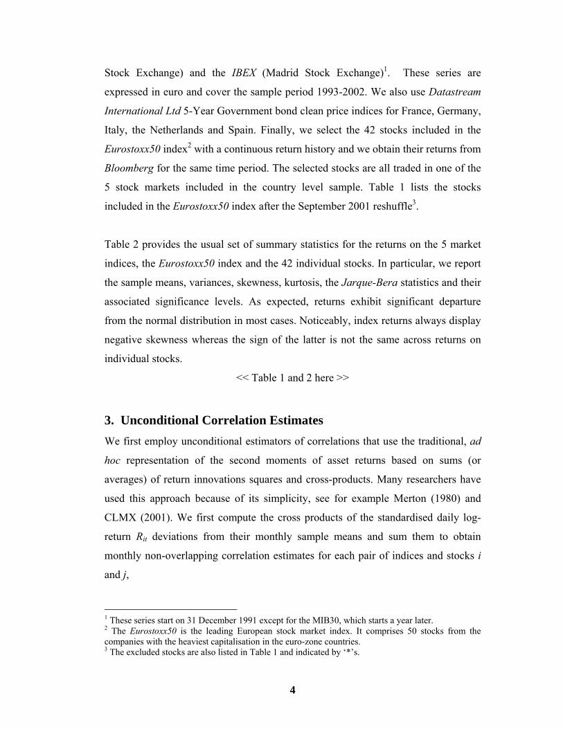
Stock Exchange) and the IBEX (Madrid Stock Exchange)1. These series are

expressed in euro and cover the sample period 1993-2002. We also use Datastream

International Ltd 5-Year Government bond clean price indices for France, Germany,

Italy, the Netherlands and Spain. Finally, we select the 42 stocks included in the

Eurostoxx50 index2 with a continuous return history and we obtain their returns from

Bloomberg for the same time period. The selected stocks are all traded in one of the

5 stock markets included in the country level sample. Table 1 lists the stocks

included in the Eurostoxx50 index after the September 2001 reshuffle3.

Table 2 provides the usual set of summary statistics for the returns on the 5 market

indices, the Eurostoxx50 index and the 42 individual stocks. In particular, we report

the sample means, variances, skewness, kurtosis, the Jarque-Bera statistics and their

associated significance levels. As expected, returns exhibit significant departure

from the normal distribution in most cases. Noticeably, index returns always display

negative skewness whereas the sign of the latter is not the same across returns on

individual stocks.

<< Table 1 and 2 here >>

3. Unconditional Correlation Estimates We first employ unconditional estimators of correlations that use the traditional, ad

hoc representation of the second moments of asset returns based on sums (or

averages) of return innovations squares and cross-products. Many researchers have

used this approach because of its simplicity, see for example Merton (1980) and

CLMX (2001). We first compute the cross products of the standardised daily log-

return Rit deviations from their monthly sample means and sum them to obtain

monthly non-overlapping correlation estimates for each pair of indices and stocks i

and j,

1 These series start on 31 December 1991 except for the MIB30, which starts a year later. 2 The Eurostoxx50 is the leading European stock market index. It comprises 50 stocks from the companies with the heaviest capitalisation in the euro-zone countries. 3 The excluded stocks are also listed in Table 1 and indicated by ‘*’s.

4

∑ −∑ −

−∑ −=

=+−

=+−

+−=

+−

21

1

2,1,

221

1,1,

,1,

21

1,1,

,,

)()(

)()(

ktjktj

ktikti

tjktjk

tikti

tji

RRRR

RRRRc (1)

We then average correlations across market indices and stocks to compute a

synthetic equally weighted index of their average correlation.

CORRt = ∑ ∑= =

n

i

n

jtjicnn1 1

,,11

(2)

Here, n is either the number of national market indices or of stocks. In Figure 1 we

plot the monthly average correlation amongst the country indexes and the individual

stocks. The former has been computed applying (1) and (2) to our country index data

with n = 5. This series shows a strong tendency to rise over time. The average stock

correlation series has been computed applying (1) and (2) to our stock data with n =

42. This series does not show any strong tendency to rise over time but rather

appears very noisy and persistent. It takes a substantial amount of time to revert to a

fairly stable long run mean (in the region of 20 percent) around which it oscillates.

<< Figure 1 >>

Unit Root Tests

To test for the presence of a stochastic time trend, we conduct Dickey-Fuller (DF)

and augmented Dickey-Fuller (ADF) tests allowing for up to 12 lags. As pointed out

by Pesaran (1997), however, there is a size-power trade-off depending on the order

of augmentation, and we consequently rely on the results provided by the tests

performed at the lower orders of augmentation. As reported in Panel A of Table 3,

the DF and ADF tests reject the null of a unit root at the 5 percent level of

significance for average stock correlation. For the average correlation amongst the 5

Euro area stock market indexes, we cannot reject the null of a unit-root in the ADF

test with 2 orders of augmentation and no deterministic time trend. However, using

an F-test and the appropriate non-standard asymptotic distribution (Hamilton

5

(1994)), we can reject at the 1 percent level the joint hypothesis that the

deterministic time trend is equal to zero and that there is a unit root. We therefore

conclude that both correlation series are stationary and, in particular, aggregate

market index correlation is trend-stationary.

Wald-Type Tests

To check on the possible presence of a deterministic time-trend, we regress our

constructed average correlations series on the latter. However, the residuals of a

static model that includes among the regressors only a constant and a deterministic

time-trend are auto-correlated, as suggested by the Durbin-Watson (DW) statistic.

We therefore estimate a dynamic model that also includes the first lag of the

dependent variable. We then conduct Wald-type tests of the restriction that the

deterministic time trend coefficient is zero using Newy-West adjusted variance-

covariance matrices to correct for heteroschedasticity and autocorrelation. Panel B

of Table 4 presents the results. The time trend coefficient is large and significant

only for average country index correlation. It explains an increase in the latter of

about 2.5 percent per year. However, the Durbin’s h4 statistic suggests that the

residuals are not serially independent. Therefore, we treat this trend coefficient

estimate with caution.

<< Table 3 >>

3. Conditional Correlations Thus far we have applied an unconditional estimation methodology. This strategy

has yielded useful insights but it has the main shortcomings that, while the average

of squares and cross-products are consistent estimators of the second moments of the

return distributions, they might be biased in small samples since they are ad hoc

representations of the volatility and correlation processes. Moreover, the aggregation

of daily data into lower frequency monthly data leads to a potential small sample 4 In the presence of lagged values of the dependent variables the DW test is biased toward acceptance of the null of no error auto-correlation. We therefore test for serial correlation of the error terms using Durbin’s (1970) h-test. We use the generalised version of this test, developed by Godfrey and Breusch, based on a general Lagrange Multiplier test. Even though this procedure can detect higher order serial correlation, we only test the null of no first-order residual autocorrelation.

6

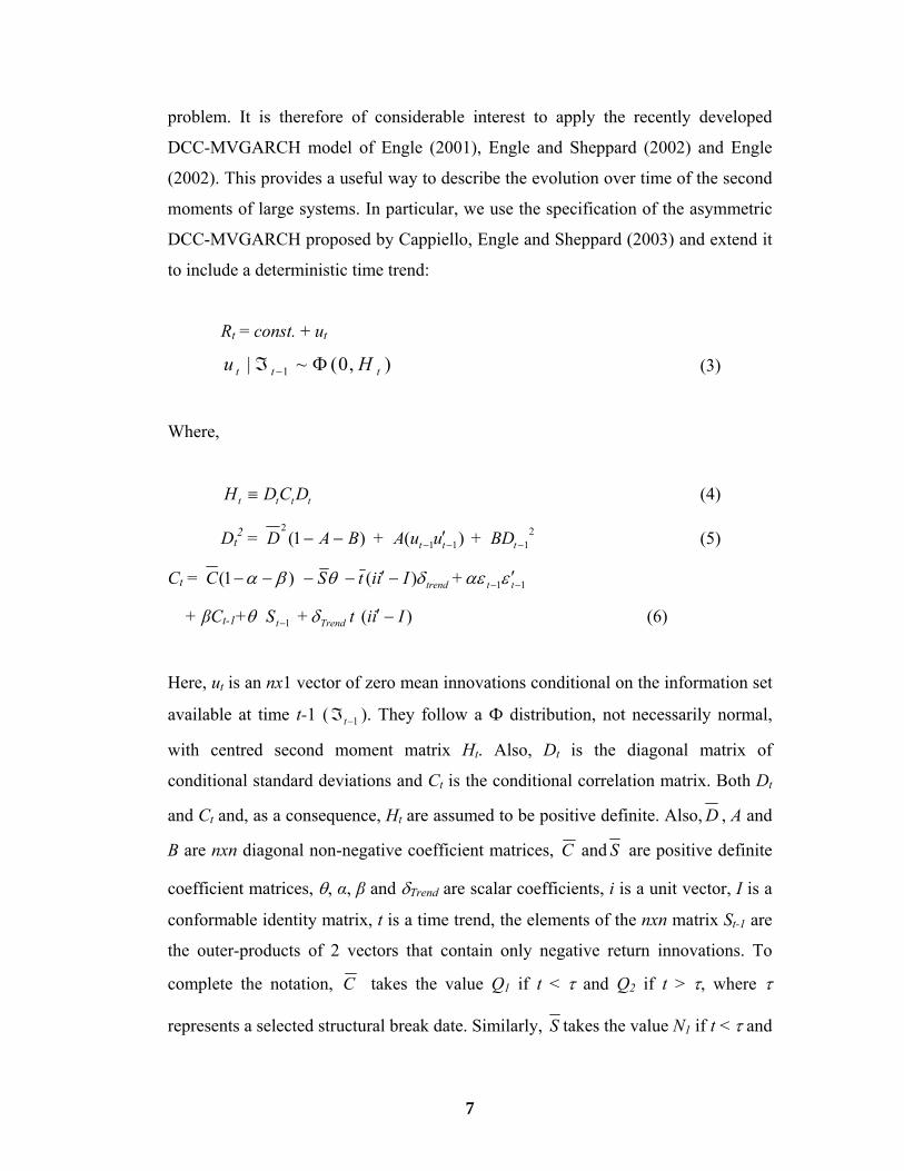
problem. It is therefore of considerable interest to apply the recently developed

DCC-MVGARCH model of Engle (2001), Engle and Sheppard (2002) and Engle

(2002). This provides a useful way to describe the evolution over time of the second

moments of large systems. In particular, we use the specification of the asymmetric

DCC-MVGARCH proposed by Cappiello, Engle and Sheppard (2003) and extend it

to include a deterministic time trend:

Rt = const. + ut

(3) ),0(~| 1 ttt Hu Φℑ −

Where,

(4) tttt DCDH ≡

Dt2 = )1(

2BAD −− + )( 11 −− ′tt uuA + (5) 2

1−tBD

Ct = )1( βα −−C θS− trendIiit δ)( −′− + 11 −− ′tt εαε

+ βCt-1+ +1−tSθ Trendδ t )( Iii −′ (6)

Here, ut is an nx1 vector of zero mean innovations conditional on the information set

available at time t-1 ( ). They follow a Ф distribution, not necessarily normal,

with centred second moment matrix H

1−ℑt

t. Also, Dt is the diagonal matrix of

conditional standard deviations and Ct is the conditional correlation matrix. Both Dt

and Ct and, as a consequence, Ht are assumed to be positive definite. Also, D , A and

B are nxn diagonal non-negative coefficient matrices, C and S are positive definite

coefficient matrices, θ, α, β and δTrend are scalar coefficients, i is a unit vector, I is a

conformable identity matrix, t is a time trend, the elements of the nxn matrix St-1 are

the outer-products of 2 vectors that contain only negative return innovations. To

complete the notation, C takes the value Q1 if t < τ and Q2 if t > τ, where τ

represents a selected structural break date. Similarly, S takes the value N1 if t < τ and

7

the value N2 if t >τ, t is the mid point of the sample period (the unconditional

sample average of the values taken by the time trend variable).

To see why the inclusion of the deterministic time trend requires this specification,

consider for simplicity but without loss of generality the univariate case of a

GARCH(1,1) with deterministic time trend,

. Taking unconditional expectations and

using the law of iterated expectations, the unconditional variance is:

tEE trendttttt δεβαεγε +++= −−−− )()( 212

21

21

tE

tEEE

trend

trendtt

δεβαγ

δεβαγε

+++=

+++= −

)()(

)()()()(2

21

2

(7)

Therefore, βα

δγε−−

+=

1)()( 2 tE trend

t and tE trendt δβαεγ −−−= )1)(( 2 . The specification

in (6) is a generalization to the multivariate case of this result.

The elements along the main diagonal of the matrix D can be seen as the long-run,

baseline levels to which conditional variances mean-revert. The matrices C and S

can be seen as the long-run, baseline levels to which the conditional correlations of

the return innovations and of the negative return innovations respectively mean-

revert5. To hasten the estimation procedure, D and C can be set equal to the

unconditional variance and correlation matrix over the sample, Q1 and Q2 can be set

equal to the sample average of 11 −− ′tt εε before and after the date τ and N1 and N2 are

the sample average of St-1 before and afterτ (in this case, the estimated conditional

correlation matrix is not guaranteed to be positive-definite). When the coefficient θ

is not constrained to be zero, the correlation process can be asymmetric. A

symmetric DCC model gives higher tail dependence for both upper and lower tails

of the multiperiod joint density. An asymmetric DCC gives higher tail dependence

in the lower tail of the multi-period density.

5 I estimate this using the sample average of the negative return innovation cross-products.

8

Engle (2001), Engle and Sheppard (2002) and Engle (2002) propose maximising the

log-likelihood function of (3) in two steps to overcome the well-known

computational problems of MVGARCH models. They first maximise the log-

likelihood with respect to the parameters that govern the process of Dt. This can be

done by estimating univariate models6 of the returns on each stock nested within a

univariate GARCH model of their conditional variance. They then suggest

maximising the second part of the likelihood function over the parameters of the

process of Ct, conditional on the estimated Dt. Preliminarily, this entails

standardising ut by the estimated Dt to obtain the nx1 vector εt7. Engle (2001), Engle

and Sheppard (2002) and Engle (2002) show that this two-stage procedure yields

consistent maximum likelihood parameter estimates, and that the inefficiency in the

two-stage estimation process can be taken into account by modifying the asymptotic

covariance of the correlation estimation parameters.

Tables 4 presents our ADCC-MVGARCH model quasi-maximum likelihood

estimates using daily data on the 5 market indices. We first estimate a simple

restricted symmetric specification of (6) with a deterministic time trend but no

structural break. We label this specification Model 1. The estimated deterministic

time trend coefficient turns out to be statistically significant but very small. Since it

is economically negligible, we drop it from all subsequent specifications. We

therefore estimate Model 2, which imposes on Model 1 the restriction that the time

trend coefficient is zero.

<< Table 4 >>

Considering the clear rise in average market index correlation visible in Figure 1,

together with the lack of evidence of a significant deterministic time trend, we then 6 The presence of an intercept term ensures that the estimated residuals are zero-mean random variables. 7 As noted by Cappiello, Engle and Sheppard (2003), standardising return innovations largely removes their departures from normality. This justifies the assumption that the standardised returns innovations εt are multivariate normal, even though the skewness, kurtosis and JB statistics reported in Table 2 imply a non-normal distribution of raw returns.

9

test for the presence of either a stochastic trend or a structural break. To check the

stationarity of the correlation process, we test the restriction that the news and

persistence parameters α and β sum to unity. The relevant LR test statistic and the

associated significance level are reported at the bottom of Table 4 (Model 2 against

Model 3). We reject the restriction that the parameters of the correlation process

sum to unity and we conclude, therefore, that the correlation process is stationary.

A structural break in the market index correlation process might, however, explain

both the strong persistence of the series and its sharp increase over the sample

period. In order to identify the structural break date, we seek guidance from

Government bond yields8. The plot of the likelihood of an ADCC-GARCH model of

the Government bond index returns as a function of 30 successive structural break

dates, as reported in Figure 2, peaks at the beginning of 1998. We also experimented

with various possible structural break dates directly in the correlations process of the

stock market indices. The model with a structural break date in January 1998

displays again the largest likelihood9. This hypothesis about the timing of the

structural break occurrence is intuitively appealing since it is roughly 12 months

before the official introduction of the Euro and thus it accounts for the likely

possibility that financial markets started to discount it in the price formation

mechanism somewhat in advance.

<< Figure 2 >>

Therefore, we finally settled on the beginning of January 1998, as this date

maximise the likelihood of a ADCC-GARCH model of the bond index returns, it

almost exactly splits our sample in half and allows for the possibility that stock

8 A necessary condition for the parity of expected real rates of returns is that bond yields differentials reflect inflation differentials. Under this perspective and neglecting differences in risk premia across countries, a structural break in Euro area interest rates correlations due to monetary policy convergence is a likely cause for a structural break in correlations at the stock market index level. This is also suggested, for example, by the study of Cappiello, Engle and Sheppard (2003) and of Hardouvelis, Malliaropulos and Priestley (2000). 9 Results for the other models are not reported to save space (they are a long list of structural break dates and corresponding likelihood function values) but they are available upon request.

10

markets discount rates might have reflected the expectation of monetary policy

convergence and increased financial integration prior to the introduction of the new

currency. Using the usual LR test statistic, reported at the bottom of Table 5, we

therefore tests Model 4 that allows for a structural break in 1998 against Model 2,

the restricted model with no structural break. We can reject this restriction at the

0.020 significance level. Moreover, once we allow for the structural break, the

restriction that the asymmetric component coefficient θ is equal to zero (Model 5

against Model 4) cannot be rejected at the 5 percent level. The coefficient θ is only

marginally significant. Its size however is non negligible from an economic point of

view. In particular, its point estimate is 45 times as large as the news reaction

parameter α.

We therefore conclude that the aggregate correlation between the 5 Euro-zone stock

market indices and the Eurostoxx50 index is best explained by a DCC-GARCH

process with a structural break in its mean10 and, perhaps, an asymmetric reaction

component. Figure 3 plots the market index average conditional correlation

estimated with the symmetric Model 5, allowing for a structural break in 1998.

<< Figure 3 >>

Turning to the correlation patterns at a more disaggregated level, the estimation

results for the 42 individual stocks are shown in Table 5. The estimated θ is very

small and the restriction that it is equal to zero11 cannot be rejected at any

conventional significance level. The time series of the estimated symmetric average

conditional industry, sector and stock return correlation is plotted in Figure 4. The

plot for the asymmetric case is almost identical.

10 We also estimated each model with the Eurostoxx50 index, and over the longer sample period 1992-2002, excluding the MIB30 index (because its series starts a year later). We obtained very similar results in all cases, and these are not reported here for brevity. 11 We do not report estimates with a deterministic time trend because the estimation procedure did not converge.

11

<< Table 5 and Figure 4 >>

As a specification check, we apply the Engle and Ng (1993) test in a multivariate

setting to our country-level MV-ADCC and MV-DCC GARCH models. Originally,

this test was designed as a diagnostic check for univariate volatility models and its

aim is to examine whether there is residual predictability in squared standardised

conditional errors using some variables observed in the past which are not included

in the volatility model. Since multivariate variance-covariance models provide

estimates of all the ingredients that are needed to compute the conditional portfolio

volatility if asset weights are known, we can use our first and second step MV-

ADCC and MV-DCC GARCH conditional volatility and correlation estimates to

compute the conditional volatility and the conditional residuals of an equally

weighted portfolio. We can then apply the Engle and Ng (1993) test to returns on the

latter.

In particular, we apply a test that combines the Sign Bias test (that uses as regressors

dummy variables I- that take value 1 or 0 depending on weather the lagged residual

is negative or positive) and the Negative and Positive Size Bias test (that use,

respectively, lagged negative and positive standardised residuals as regressors, zt-1-

and zt-1+). As reported in Table 6, we can reject the null of non-predictability of the

squared standardised conditional residuals. Therefore, in spite of the mixed evidence

provided by the LR tests of the ADCC-MVGARCH against the DCC-MVGARCH,

distributional asymmetric are important. The latter are probably of a non-linear

nature12 and we leave the difficult quest for a better specification for future research.

12 This, as far market indices are concerned, lies in partial contrast to those reported by Cappiello, Engle and Sheppard (2003). However, since we were able to replicate their results with their same set of market indices, frequency and data period (these results are not reported for brevity and because they exactly match results already published by Cappiello, Engle and Sheppard (2003) but they are available upon request.), we conclude that the difference between our and their results is due to whether non-Euro area market indices are included. Correlations amongst Euro area market indices, in particular, appear to display a substantial lower tendency to increase following joint past negative returns than those amongst markets outside the Euro area. Another likely but less important reason for why our results differ from those of Cappiello, Engle and Sheppard (2003) with respect to the importance of asymmetric correlation reactions to past returns innovations is the different data frequency – they use only weekly data whereas we use both daily and weekly data and for the former

12

<< Table 6 >>

4. Summary and Conclusions The purpose of this paper is to contribute to the literature on the correlation

dynamics in European equity markets. Our main focus has been on country-level

market index correlations, but we also examined stock correlations for comparison

purposes. We applied the symmetric and asymmetric version of the DCC-

MVGARCH model of Engle (2001), Engle and Sheppard (2002) and Engle (2002)

to capture their behaviour over time.

We find strong evidence of a structural break in the mean shortly before the

introduction of the Euro. This explains both the strong persistence of the correlation

time series and its significant rise over the sample period. This confirms the results

reported by Cappiello, Engle and Sheppard (2003) and is consistent with the rise in

volatility spillovers noticed by Baele (2002). We also find evidence that, at the level

of the national stock market indices, the conditional correlation response to past

positive and negative news is asymmetrical. Stock correlations instead do not appear

to follow an asymmetric correlation process. These findings provide mixed support

to a popular explanation, see for example Patton (2002), for why the skewness of

market index returns is often negative whereas stock returns have either negative or

positive skewness (similar findings are reported in Table 2). More importantly,

applying a multivariate extension of the Engle and Ng (1993) test, we find that

beyond asymmetric correlation reactions to past returns innovations there must be

other, perhaps more important source of asymmetry in the distribution of asset

returns. This issue represents an important and fruitful topic for future research.

Overall, our results suggest that non-country factors drive the volatility of equity

returns. In particular, because of the rise in correlations among the largest national the importance of the asymmetric correlation component is always lower. This suggests the importance of taking into account temporal aggregation issues when modelling asset returns second moments dynamics.

13

stock markets indices, the stochastic components of the latter can now be expected

to behave almost identically (with conditional correlations being close to 100

percent as reported in Figure 3). This suggests that there is little expected benefit

from strategies that diversify across Euro-zone market indices, although

diversification across stocks remains useful. This explains why, as reported by

Eiling, Gerard and de Roon (2004), the outperformance of country-based

diversification strategies relative to industry-based strategies has disappeared after

the introduction of the Euro. As a consequence, fund managers should think through

the full ramifications of seeking cost-effective diversification in the Euro area by

adopting the passive strategy of investing in market indexes rather than a selection

of stocks or industries from the whole supra-national market.

More deeply, the dramatic increase in country level market index correlation rises

the possibility of a ‘correlation puzzle’. The relevant question from the perspective

of the informational efficiency of the market pricing mechanism is whether this

increase in return correlation is justified by increased correlation in fundamentals

and discount rates. Adjaountè and Danthine (2001) document a significant increase

in correlations between Euro area country equity indices. However, they find the

same increase after they adjust for currency effects, thus suggesting that the

elimination of currency risk is not the main cause. De Santis, Gerard and Hillion

(1999) show similar results. While Adjaountè and Danthine (2004) report

preliminary evidence of convergence of economic fundamentals such as gross

domestic product growth rates, little or no direct evidence is available on discount

rates and on equity fundamentals such as dividend growth rates. Expanding this

body of evidence is a fruitful area for future research.

14

Bibliography

Adjaouté, K., Danthine J.P., 2001. EMU and Portfolio Diversification Opportunities, CEPR discussion paper No. 2962. Adjaouté, K., Danthine J.P., 2004. Equity Returns and Integration: Is Europe Changing?, FAME Research Paper N° 117. Ang, A., Bekaert, G., 1999. International Asset Allocation with Time-Varying Correlations, NBER Working Paper No. 7056. Baks, K.P., Metrick, A., Wachter, J., 2001. Should Investors Avoid All Actively Managed Mutual Funds? A Study in Bayesian Performance Evaluation. Journal of Finance 56, 45-85. Baele, L., 2002. Volatility Spillover Effects in European Equity Markets: Evidence from a Regime-Switching Model, Working Paper. Blake, D., Timmerman, A., 1998. Mutual Fund Performance: Evidence from the UK. European Finance Review 2, 57-77. Campbell, J.Y, Lettau, M., Malkiel, B.G., XU, Y., 2001. Have Individual Stocks Become More Volatile? An Empirical Exploration Of Idiosyncratic Risk. Journal of Finance 56, 1-43. Cappiello, L., Engle, R.F., Sheppard, K., 2003. Asymmetric Dynamics in the Correlations of Global Equity and Bond Returns. ECB Working Paper No. 204. Coval, J.D., Moskowitz, T.J., 2001. The Geography of Investment: Informed Trading and Asset Prices. Journal of Political Economy.109, 811-841. De Santis, G., Gerard, B., 1997. International Asset Pricing and Portfolio Diversification with Time-Varying Risk. Journal of Finance 52, 1881-1912. De Santis, G., Gerard B. Hillion P., 1999. International Portfolio Management, Currency Risk and the Euro, forthcoming Journal of Banking and Finance Dickey, D.A., Fuller, W.A., 1979. Distribution of the Estimators for Auto-regressive Time Series with a Unit Root. Journal of the American Statistical Association 74, 427-31. Durbin, J., 1970. Testing for Serial Correlation in Least Squares Regression when Some of the Regressors are Lagged Dependent Variables. Econometrica 38, 410-421. Eiling, E., Gerard, B. de Roon F., 2004. Asset Allocation in the Euro-zone: Industry or Country Based?, unpublished manuscript. Engle, R.F., 2001. Dynamic Conditional Correlation – A Simple Class of Multivariate GARCH Models. Working Paper, University of California, San Diego. Engle, R.F., 2002. Dynamic Conditional Correlation: A Simple Class of Multivariate Generalised Autoregressive Conditional Heteroskedasticity Models. Journal of Business and Economic Statistic 20, 339-350.

15

Engle, R.F. and Ng, V.K., 1993. Measuring and Testing the Impact of news on Volatility. Journal of Finance 48, 1749-1777. Engle, R.F., Sheppard, K., 2001. Theoretical and Empirical Properties of Dynamic Conditional Correlation Multivariate GARCH. Working Paper, University of California, San Diego. Erb, C.B., Harvey, C.R., Viskanta, T.E., 1994. Forecasting International Equity Correlations. Financial Analyst Journal 50, 32-45. Fratzschler, M., 2002. Financial Market Integration in Europe: On the Effects of Euro area on Stock Markets. International Journal of Finance and Economics 7, 165-193. Hamilton, J.D., 1994. Time Series Analysis. Princeton University Press, Princeton. Hardouvelis, G., Malliaropulos, D., Priestley, R., 2000. Euro area and European Stock Market Integration. CEPR Discussion Paper. Longin, F., Solnik, B., 1995. Is Correlation in International Equity Returns Constant: 1960 – 1990?. Journal of International Money and Finance 14, 3-26. Longin, F., Solnik, B., 2001. Extreme Correlation of International Equity Markets, Journal of Finance, 56, 649-676 Merton, R.C., 1980. On Estimating the Expected Return on the Market: an Exploratory Investigation. Journal of Financial Economics 8, 323-361. Newy, W.K., West, D.K., 1987. A Simple, Positive Semi-Definite, Heteroskedasticity and Autocorrelation Consistent Covariance Matrix. Econometrica 55, 703-8. Patton, A. J. (2002). Skewness, Asymmetric Dependence and Portfolios. Working Paper, University of California, San Diego. Pesaran, M. H., Pesaran, B., 1997. Working with Microfit 4.0. Oxford University Press, Oxford. Wermers, R., 2000. Mutual Fund Performance: An Empirical Decomposition into Stock-Picking Talent, Style, Transaction Costs, and Expenses. Journal of Finance 55, 1655-1695.

16

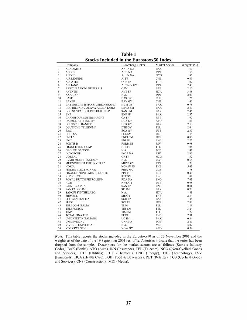
Table 1 Stocks Included in the Eurostoxx50 Index

Company Bloomberg Ticker Market Sector Weights (%) 1 ABN AMRO AABA NA BAK 1.59 2 AEGON AGN NA INN 1.55 3 AHOLD AHLN NA NCG 1.87 4 AIR LIQUIDE AI FP CHE 0.89 5 ALCATEL CGE FP THE 1.02 6 ALLIANZ ALThe V GY INN 2.49 7 ASSICURAZIONI GENERALI G IM INN 2.15 8 AVENTIS AVE FP HCA 3.48 9 AXA UAP N.A. INN 2.00 10 BASF BAS GY CHE 1.26 11 BAYER BAY GY CHE 1.40 12 BAYERISCHE HYPO & VEREINSBANK HVM GY BAK 0.75 13 BCO BILBAO VIZCAYA ARGENTARIA BBVA SM BAK 2.39 14 BCO SANTANDER CENTRAL HISP SAN SM BAK 2.46 15 BNP* BNP FP BAK 2.37 16 CARREFOUR SUPERMARCHE CA FP RET 1.97 17 DAIMLERCHRYSLER* DCX GY ATO 1.86 18 DEUTSCHE BANK R DBK GY BAK 2.13 19 DEUTSCHE TELEKOM* DTE GY TEL 2.64 20 E.ON EOA GY UTS 2.39 21 ENDESA ELE SM UTS 1.14 22 ENEL* ENEL IM UTS 0.83 23 ENI* ENI IM ENG 2.22 24 FORTIS B FORB BB FSV 0.98 25 FRANCE TELECOM* FTE FP TEL 1.06 26 GROUPE DANONE N.A. FOB 1.47 27 ING GROEP INGA NA FSV 2.95 28 L'OREAL OR FP NCG 1.52 29 LVMH MOET HENNESSY N.A. CGS 0.55 30 MUENCHENER RUECKVER R* MUV2 GY INN 1.70 31 NOKIA NOK1V FH THE 5.63 32 PHILIPS ELECTRONICS PHIA NA CGS 1.75 33 PINAULT PRINTEMPS REDOUTE PP FP RET 0.49 34 REPSOL YPF REP SM ENG 1.02 35 ROYAL DUTCH PETROLEUM RDA NA ENG 7.63 36 RWE RWE GY UTS 0.98 37 SAINT GOBAIN SAN FP CNS 0.81 38 SAN PAOLO IMI SPI IM BAK 0.70 39 SANOFI SYNTHELABO N.A. HCA 1.81 40 SIEMENS SIE GY THE 2.34 41 SOC GENERALE A SGO FP BAK 1.46 42 SUEZ SZE FP UTS 2.39 43 TELECOM ITALIA TI IM TEL 1.19 44 TELEFONICA TEF SM TEL 3.24 45 TIM* TIM IM TEL 1.22 46 TOTAL FINA ELF FP FP ENG 7.31 47 UNICREDITO ITALIANO UC IM BAK 0.84 48 UNILEVER NV UNA NA FOB 2.49 49 VIVENDI UNIVERSAL N.A. MDI 3.07 50 VOLKSWAGEN VOW GY ATO 0.54

Note. This table reports the stocks included in the Eurostoxx50 as of 23 November 2001 and the weights as of the date of the 19 September 2001 reshuffle. Asterisks indicate that the series has been dropped from the sample. Descriptors for the market sectors are as follows (Stoxx’s Industry Codes): BAK (Banks), ATO (Auto), INN (Insurance), TEL (Telecom), NCG ((Non-Cyclical Goods and Services), UTS (Utilities), CHE (Chemical), ENG (Energy), THE (Technology), FSV (Financials), HCA (Health Care), FOB (Food & Beverages), RET (Retailer), CGS (Cyclical Goods and Services), CNS (Construction), MDI (Media).

17

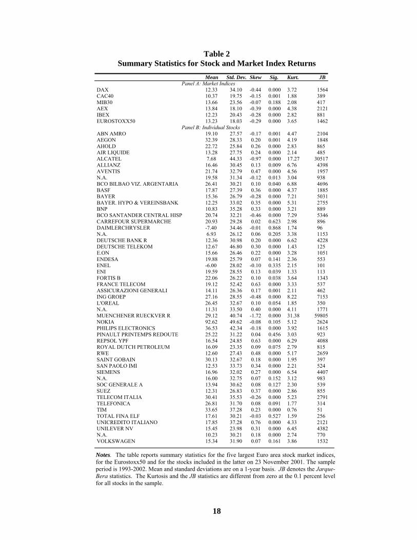
Table 2 Summary Statistics for Stock and Market Index Returns

Mean Std. Dev. Skew Sig. Kurt. JB

Panel A: Market Indices DAX 12.33 34.10 -0.44 0.000 3.72 1564 CAC40 10.37 19.75 -0.15 0.001 1.88 389 MIB30 13.66 23.56 -0.07 0.188 2.08 417 AEX 13.84 18.10 -0.39 0.000 4.38 2121 IBEX 12.23 20.43 -0.28 0.000 2.82 881 EUROSTOXX50 13.23 18.03 -0.29 0.000 3.65 1462 Panel B: Individual Stocks ABN AMRO 19.10 27.57 -0.17 0.001 4.47 2104 AEGON 32.39 28.33 0.20 0.001 4.19 1848 AHOLD 22.72 25.84 0.26 0.000 2.83 865 AIR LIQUIDE 13.28 27.75 0.24 0.000 2.14 485 ALCATEL 7.68 44.33 -0.97 0.000 17.27 30517 ALLIANZ 16.46 30.45 0.13 0.009 6.76 4398 AVENTIS 21.74 32.79 0.47 0.000 4.56 1957 N.A. 19.58 31.34 -0.12 0.013 3.04 938 BCO BILBAO VIZ. ARGENTARIA 26.41 30.21 0.10 0.040 6.88 4696 BASF 17.87 27.39 0.36 0.000 4.37 1885 BAYER 15.36 26.79 -0.28 0.000 7.21 5031 BAYER. HYPO & VEREINSBANK 12.25 33.02 0.35 0.000 5.31 2755 BNP 10.83 35.28 0.33 0.000 3.21 889 BCO SANTANDER CENTRAL HISP 20.74 32.21 -0.46 0.000 7.29 5346 CARREFOUR SUPERMARCHE 20.93 29.28 0.02 0.623 2.98 896 DAIMLERCHRYSLER -7.40 34.46 -0.01 0.868 1.74 96 N.A. 6.93 26.12 0.06 0.205 3.38 1153 DEUTSCHE BANK R 12.36 30.98 0.20 0.000 6.62 4228 DEUTSCHE TELEKOM 12.67 46.80 0.30 0.000 1.43 125 E.ON 15.66 26.46 0.22 0.000 3.28 1051 ENDESA 19.88 25.79 0.07 0.141 2.36 553 ENEL -6.00 28.02 -0.10 0.335 2.15 101 ENI 19.59 28.55 0.13 0.039 1.33 113 FORTIS B 22.06 26.22 0.10 0.038 3.64 1343 FRANCE TELECOM 19.12 52.42 0.63 0.000 3.33 537 ASSICURAZIONI GENERALI 14.11 26.36 0.17 0.001 2.11 462 ING GROEP 27.16 28.55 -0.48 0.000 8.22 7153 L'OREAL 26.45 32.67 0.10 0.054 1.85 350 N.A. 11.31 33.50 0.40 0.000 4.11 1771 MUENCHENER RUECKVER R 29.12 40.74 -1.72 0.000 31.38 59805 NOKIA 92.62 49.62 -0.08 0.105 5.12 2624 PHILIPS ELECTRONICS 36.53 42.34 -0.18 0.000 3.92 1615 PINAULT PRINTEMPS REDOUTE 25.22 31.22 0.04 0.456 3.03 923 REPSOL YPF 16.54 24.85 0.63 0.000 6.29 4088 ROYAL DUTCH PETROLEUM 16.09 23.35 0.09 0.075 2.79 815 RWE 12.60 27.43 0.48 0.000 5.17 2659 SAINT GOBAIN 30.13 32.67 0.18 0.000 1.95 397 SAN PAOLO IMI 12.53 33.73 0.34 0.000 2.21 524 SIEMENS 16.96 32.02 0.27 0.000 6.54 4407 N.A. 16.00 32.75 0.07 0.152 3.12 983 SOC GENERALE A 13.94 30.62 0.08 0.127 2.30 539 SUEZ 12.31 26.83 0.37 0.000 2.86 855 TELECOM ITALIA 30.41 35.53 -0.26 0.000 5.23 2791 TELEFONICA 26.81 31.70 0.08 0.091 1.77 314 TIM 33.65 37.28 0.23 0.000 0.76 51 TOTAL FINA ELF 17.61 30.21 -0.03 0.527 1.59 256 UNICREDITO ITALIANO 17.85 37.28 0.76 0.000 4.33 2121 UNILEVER NV 15.45 23.98 0.31 0.000 6.45 4382 N.A. 10.23 30.21 0.18 0.000 2.74 770 VOLKSWAGEN 15.34 31.90 0.07 0.161 3.86 1532 Notes. The table reports summary statistics for the five largest Euro area stock market indices, for the Eurostoxx50 and for the stocks included in the latter on 23 November 2001. The sample period is 1993-2002. Mean and standard deviations are on a 1-year basis. JB denotes the Jarque-Bera statistics. The Kurtosis and the JB statistics are different from zero at the 0.1 percent level for all stocks in the sample.

18

Figure 1 Average Market Index and Stock Correlations

0%10%20%30%40%50%

60%70%80%90%

100%

1993 1994 1995 1996 1997 1998 1999 2000 2001

Market Indices Stocks

Note. This figure plots the unconditional estimates of the averagecorrelation between the 5 largest stock market indices in the Euro areaand the average correlation between 42 stocks included in theEurostoxx50 Index over the sample period.

19

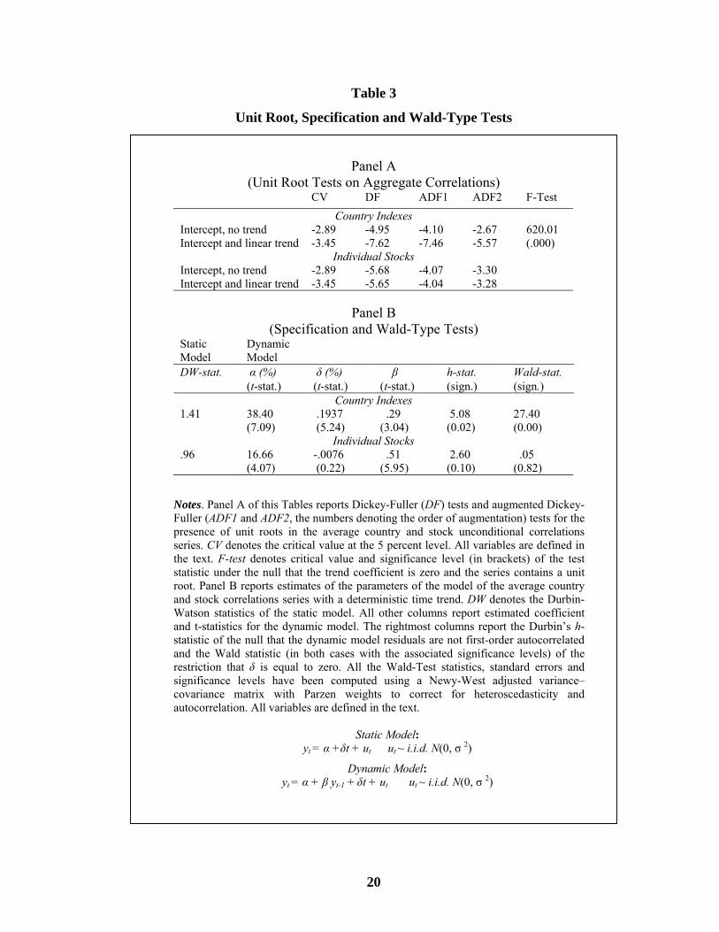
Table 3

Unit Root, Specification and Wald-Type Tests

Panel A (Unit Root Tests on Aggregate Correlations)

CV DF ADF1 ADF2 F-Test Country Indexes

Intercept, no trend Intercept and linear trend

-2.89 -3.45

-4.95 -7.62

-4.10 -7.46

-2.67 -5.57

620.01 (.000)

Individual Stocks Intercept, no trend Intercept and linear trend

-2.89 -3.45

-5.68 -5.65

-4.07 -4.04

-3.30 -3.28

Panel B

(Specification and Wald-Type Tests) Static Model

Dynamic Model

DW-stat. α (%) (t-stat.)

δ (%) (t-stat.)

β (t-stat.)

h-stat. (sign.)

Wald-stat. (sign.)

Country Indexes 1.41 38.40

(7.09) .1937 (5.24)

.29 (3.04)

5.08 (0.02)

27.40 (0.00)

Individual Stocks .96 16.66

(4.07) -.0076 (0.22)

.51 (5.95)

2.60 (0.10)

.05 (0.82)

Notes. Panel A of this Tables reports Dickey-Fuller (DF) tests and augmented Dickey-Fuller (ADF1 and ADF2, the numbers denoting the order of augmentation) tests for the presence of unit roots in the average country and stock unconditional correlations series. CV denotes the critical value at the 5 percent level. All variables are defined in the text. F-test denotes critical value and significance level (in brackets) of the test statistic under the null that the trend coefficient is zero and the series contains a unit root. Panel B reports estimates of the parameters of the model of the average country and stock correlations series with a deterministic time trend. DW denotes the Durbin-Watson statistics of the static model. All other columns report estimated coefficient and t-statistics for the dynamic model. The rightmost columns report the Durbin’s h-statistic of the null that the dynamic model residuals are not first-order autocorrelated and the Wald statistic (in both cases with the associated significance levels) of the restriction that δ is equal to zero. All the Wald-Test statistics, standard errors and significance levels have been computed using a Newy-West adjusted variance–covariance matrix with Parzen weights to correct for heteroscedasticity and autocorrelation. All variables are defined in the text.

Static Model: yt = α +δt + ut ut ~ i.i.d. N(0, σ 2)

Dynamic Model: yt = α + β yt-1 + δt + ut ut ~ i.i.d. N(0, σ 2)

20

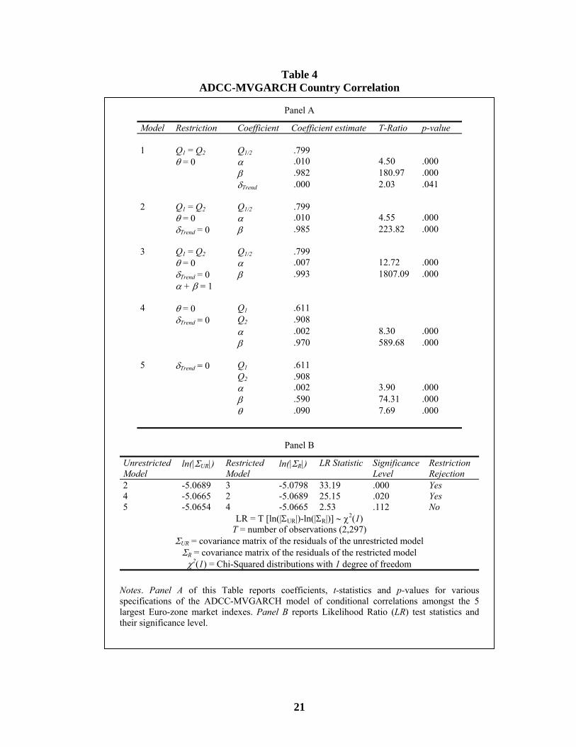
Table 4 ADCC-MVGARCH Country Correlation

Panel A

Model Restriction Coefficient Coefficient estimate T-Ratio p-value 1 Q1 = Q2 Q1/2 .799 θ = 0 α .010 4.50 .000 β .982 180.97 .000 δTrend .000 2.03 .041 2 Q1 = Q2 Q1/2 .799 θ = 0 α .010 4.55 .000 δTrend = 0 β .985 223.82 .000 3 Q1 = Q2 Q1/2 .799 θ = 0 α .007 12.72 .000 δTrend = 0 β .993 1807.09 .000 α + β = 1 4 θ = 0 Q1 .611 δTrend = 0 Q2 .908 α .002 8.30 .000 β .970 589.68 .000 5 δTrend = 0 Q1 .611 Q2 .908 α .002 3.90 .000 β .590 74.31 .000 θ .090 7.69 .000

Panel B

Unrestricted Model

ln(|ΣUR|) Restricted Model

ln(|ΣR|) LR Statistic Significance Level

Restriction Rejection

2 -5.0689 3 -5.0798 33.19 .000 Yes 4 -5.0665 2 -5.0689 25.15 .020 Yes 5 -5.0654 4 -5.0665 2.53 .112 No

LR = T [ln(|ΣUR|)-ln(|ΣR|)] ∼ χ2(1) T = number of observations (2,297)

ΣUR = covariance matrix of the residuals of the unrestricted model ΣR = covariance matrix of the residuals of the restricted model χ2(1) = Chi-Squared distributions with 1 degree of freedom

Notes. Panel A of this Table reports coefficients, t-statistics and p-values for variousspecifications of the ADCC-MVGARCH model of conditional correlations amongst the 5largest Euro-zone market indexes. Panel B reports Likelihood Ratio (LR) test statistics andtheir significance level.

21

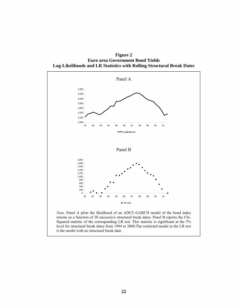
Figure 2 Euro area Government Bond Yields

Log-Likelihoods and LR Statistics with Rolling Structural Break Dates

Panel A

2,000

2,200

2,400

2,600

2,800

3,000

3,200

3,400

91 92 93 94 95 96 97 98 99 00 01

Loglikelihood

Panel B

0200400600800

1,0001,2001,4001,6001,8002,000

91 92 93 94 95 96 97 98 99 00 01

Chi-stat.

Note. Panel A plots the likelihood of an ADCC-GARCH model of the bond indexreturns as a function of 30 successive structural break dates. Panel B reports the Chi-Squared statistic of the corresponding LR test. This statistic is significant at the 5%level for structural break dates from 1994 to 2000.The restricted model in the LR testis the model with no structural break date.

22

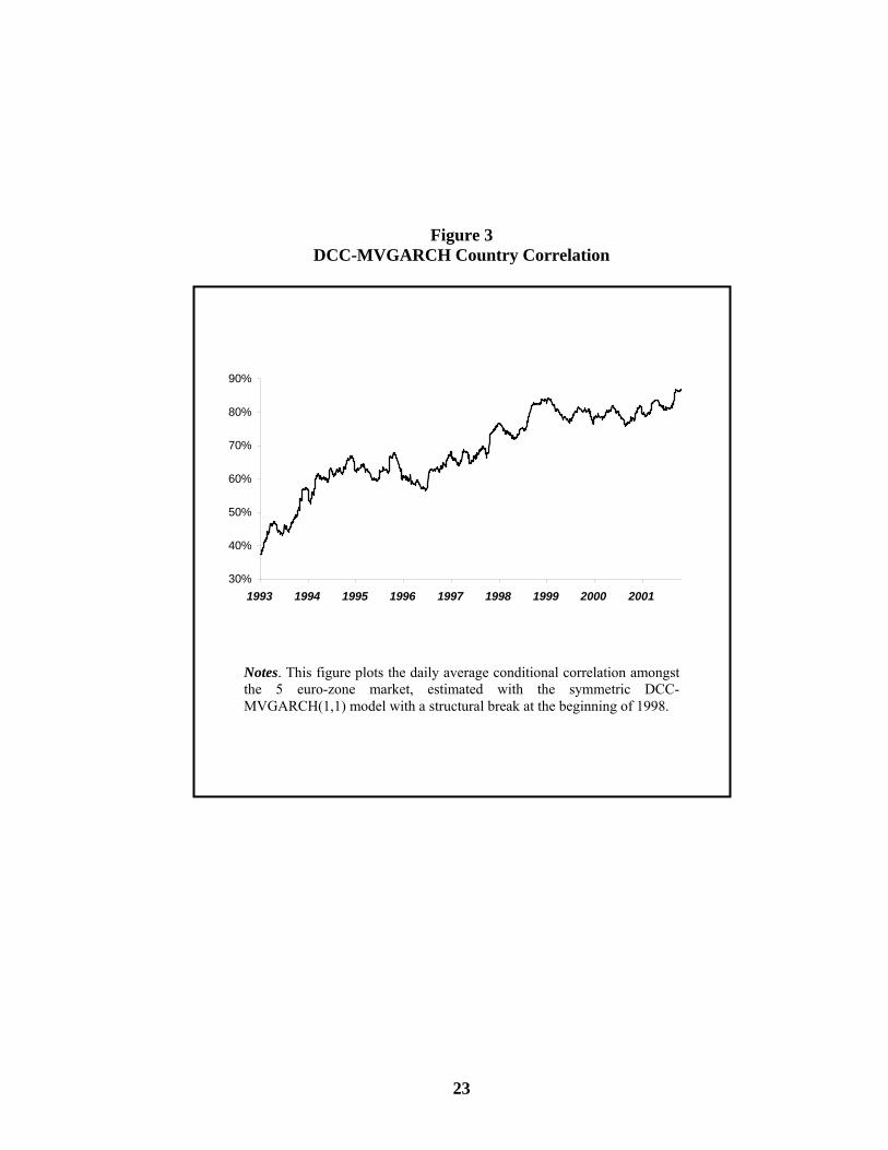
Figure 3 DCC-MVGARCH Country Correlation

30%

40%

50%

60%

70%

80%

90%

1993 1994 1995 1996 1997 1998 1999 2000 2001

Notes. This figure plots the daily average conditional correlation amongstthe 5 euro-zone market, estimated with the symmetric DCC-MVGARCH(1,1) model with a structural break at the beginning of 1998.

23

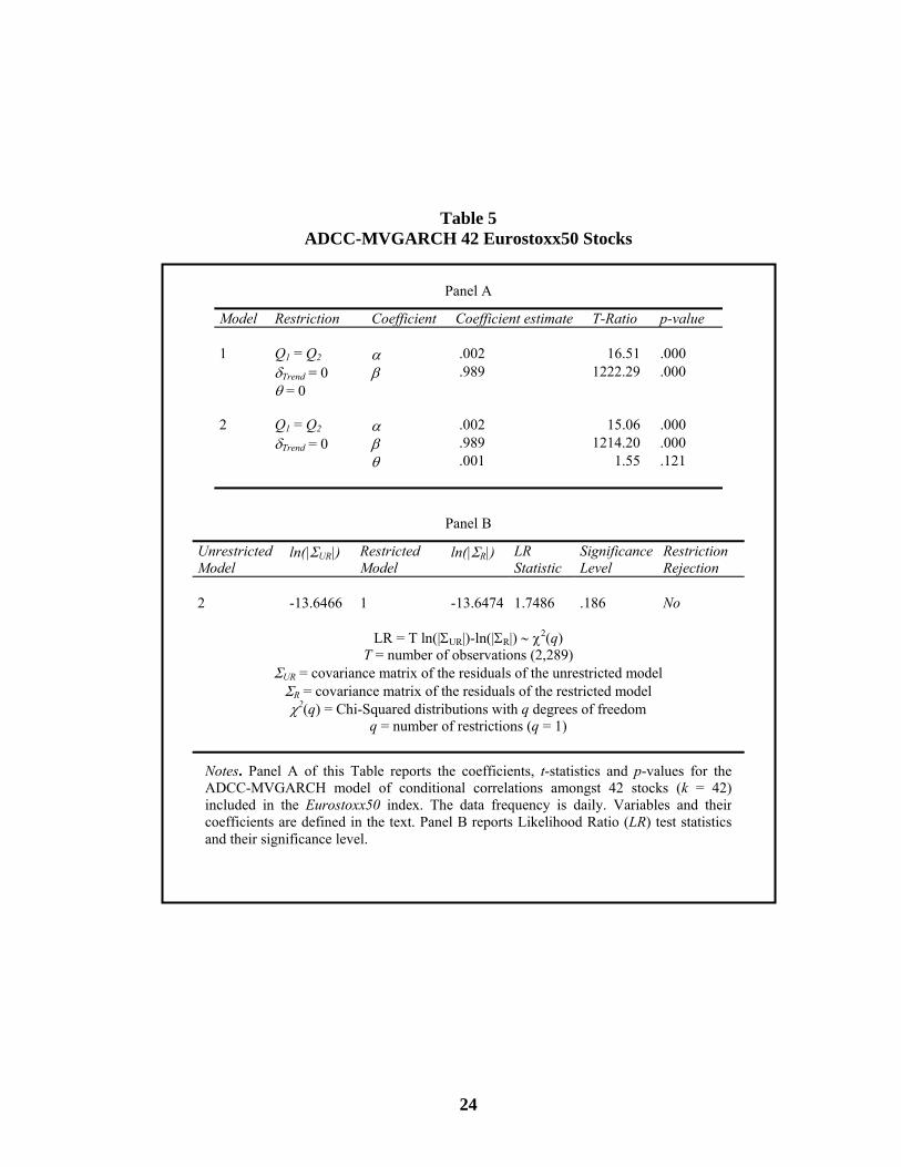
Table 5 ADCC-MVGARCH 42 Eurostoxx50 Stocks

Panel A

Model Restriction Coefficient Coefficient estimate T-Ratio p-value

1 Q1 = Q2 α .002 16.51 .000 δTrend = 0 β .989 1222.29 .000 θ = 0 2 Q1 = Q2 α .002 15.06 .000 δTrend = 0 β .989 1214.20 .000 θ .001 1.55 .121

Panel B

Unrestricted Model

ln(|ΣUR|) Restricted Model

ln(|ΣR|) LR Statistic

Significance Level

Restriction Rejection

2 -13.6466 1 -13.6474 1.7486 .186 No

LR = T ln(|ΣUR|)-ln(|ΣR|) ∼ χ2(q) T = number of observations (2,289)

ΣUR = covariance matrix of the residuals of the unrestricted model ΣR = covariance matrix of the residuals of the restricted model χ2(q) = Chi-Squared distributions with q degrees of freedom

q = number of restrictions (q = 1)

Notes. Panel A of this Table reports the coefficients, t-statistics and p-values for theADCC-MVGARCH model of conditional correlations amongst 42 stocks (k = 42)included in the Eurostoxx50 index. The data frequency is daily. Variables and theircoefficients are defined in the text. Panel B reports Likelihood Ratio (LR) test statisticsand their significance level.

24

Figure 4

DCC-MVGARCH Stock Correlations

27%

29%

31%

33%

35%

37%

1993 1994 1995 1996 1997 1998 1999 2000 2001

Model

DCC

Notes. Thand Ng (1

Notes. This figure plots the daily average conditional correlation amongst42 individual stocks included in the Eurostoxx50 index, estimated with thesymmetric DCC-MVGARCH(1,1).

Table 6

Diagnostic Tests

S-

[sig.] u-

[sig.] u+

[sig.] Chi-

squared(3) [sig.]

Country Indices - Daily

.068 [.394]

-.123 [.039]

-.142 [.058]

29.64 [.000]

is Table reports the coefficients and p-values for a multivariate application of the Engle993) test. Variables and their coefficients are defined in the text.

25