Testing for predictability in emerging equity markets

www.elsevier.com/locate/econbase

Emerging Markets Review 5 (2004) 295–316

Testing for predictability in emerging equity markets

Eui Jung Chang, Eduardo Jose Araujo Lima,Benjamin Miranda Tabak*

Banco Central do Brasil, SBS Quadra 3, Bloco B., Ed. Sede, 9 andar, Brasilia, DF 70074-900, Brazil

Received 1 November 2003; received in revised form 1 March 2004; accepted 1 March 2004

Available online 4 August 2004

Abstract

In this paper we test whether returns for emerging stock markets are predictable. We analyze

predictability by means of multivariate variance ratios using heteroscedastic robust bootstrap

procedures. Empirical results suggest that emerging equity indices do not resemble a random walk

while for developed country indices (US and Japan) we are not able to reject this hypothesis.

Furthermore, by employing variable moving average (VMA) and trading range break (TRB)

technical trading rules we show that there is some evidence of forecasting power. However, when we

take into account trading costs and a buy and hold strategy, only a few rules generate positive excess

returns. We check for robustness by analyzing returns from 1559 different trading rules, testing

different sub-samples, analyzing returns in bear and bull markets, and also comparing results found

for emerging markets to the US and Japan. Furthermore, for the US the Variable Moving Average

trading rules suggested in Brock et al. [J. Finance 47 (1992) 1731] do not seem to have forecasting

power for the recent sample used, which could be due to the fact that these rules have been widely

employed by market participants having the potential abnormal gains from them disappear.

D 2004 Elsevier B.V. All rights reserved.

JEL classification: G12; G14; G15

Keywords: Technical analysis; Emerging stock markets; Predictability

1. Introduction

Emerging markets have received massive inflows of capital in the past and have

become interesting alternatives for investors seeking diversification. Indeed, Harvey

(1995) shows that emerging markets provide investment opportunities for world

1566-0141/$ - see front matter D 2004 Elsevier B.V. All rights reserved.

doi:10.1016/j.ememar.2004.03.005

* Corresponding author. Tel.: +55-61-414-3092; fax: +55-61-414-3045.

E-mail address: [email protected] (B.M. Tabak).

E.J. Chang et al. / Emerging Markets Review 5 (2004) 295–316296

investors. In general, emerging markets offer high expected returns with an associated

high risk.

The aim of this paper is to assess whether emerging stock markets in Latin America and

Asia exhibit predictability by testing the random walk hypothesis (RWH) using a

multivariate version of the variance ratio (VR) test with a heteroscedastic robust bootstrap

procedure and by testing technical trading rules such as the variable moving average

(VMA) and trading range break (TRB) levels. We study Argentina, Brazil, Chile and

Mexico in Latin America, and India, Indonesia, Korea, Malaysia, the Philippines, Thailand,

and Taiwan in Asia. We also present results for Japan and the US for comparison purposes.1

Most papers use variable and fixed moving average trading rules to assess whether

there are significant profits to be made by technical analysis, following the seminal paper

of Brock et al. (1992). The current paper analyzes whether technical analysis possesses

forecasting power for price changes by studying the forecast power of 1559 different

trading rules using a bootstrap procedure. The VMA technical trading rules proposed by

Brock et al. (1992) are used as a benchmark.2 We also test trading rules using TRB levels.

Furthermore, the analysis is performed on a very recent sample—the period from January

1991 through January 2004—in which most countries have liberalized their current

accounts and received massive foreign portfolio inflows. We compare sub-samples (before

and after the Asian crisis) and check whether the results are robust to the period used in the

analysis. We also study the results of trading rules in bear and bull sub-samples.3

The remainder of the paper is organized as follows. Section 2 presents a brief literature

review. The empirical methodology is discussed in Section 3. In Section 4 we describe the

data and the sample used in this paper. Section 5 shows empirical results. Finally, Section

6 concludes the paper.

2. Brief literature review

If a stock price does satisfy the RWH, it follows that future equity prices are not

predictable based on past prices. This has important implications for asset pricing

modeling, especially for traders and practitioners that are searching for patterns in prices

and betting on the markets using these patterns.

Lo and MacKinlay (1988), in a seminal paper, present evidence that the RWH is

strongly rejected by using VR statistics for the sample period 1962–1985 and for different

subperiods.4 Since their seminal work, a variety of papers have found mixed evidence for a

number of countries and sample periods.5

1 International comparisons such as those presented in Harvey (1995) provide evidence that emerging

markets returns are generally more predictable than the developed market returns.2 Brock et al. (1992) propose the use of 1_50, 1_150, 1_200, 5_150 and 2_200 VMA. The first observation is

the length of the short-term moving average while the second one is the length of the long-term moving average.3 Although these bull and bear markets are defined on an ex-post basis they are useful in understanding why

even if trading rules do not perform well for the full sample, they still are widely employed around the world by

investors and traders. There could be substantial differences in the excess returns in these periods, which could

explain their relative success.4 Lo and MacKinlay (1989) show that these VR statistics are more reliable than traditional unit root tests.5 See Frennberg and Hansson (1993) and Ayadi and Pyun (1994) for applications of this methodology for the

Swedish and Korean equity markets, respectively.

E.J. Chang et al. / Emerging Markets Review 5 (2004) 295–316 297

Urrutia (1995) tests the RWH for Latin American emerging equity markets and rejects

it for some of these countries, suggesting that there is predictability. In another paper,

Huang (1995) also shows that we can reject the RWH for Korea, Malaysia, Hong Kong,

Singapore and Thailand.6

Another branch of the literature focuses on the predictability of price changes

using technical trading rules and determines whether one can earn abnormal profits

from them, even when taking into account trading costs relative to a buy and hold

strategy.

In a seminal paper, Brock et al. (1992) test technical trading rules for the U.S. equity

market. Their results are consistent with technical rules having predictive power. The

authors suggest that technical rules may pick up some of the hidden patterns that are

not detected by simple linear models.7 They find that the returns during buy periods are

statistically larger than those during sell periods, and that the former are less volatile.8

Ratner and Leal (1999) analyze technical trading rules for 10 emerging equity markets

from January 1982 through April 1995. Similarly to Bessembinder and Chan (1995),

these authors have found using 10 VMA rules that for Taiwan, Thailand, and Mexico

there were substantial profits to be made.9 Additionally, Genc� ay (1998), Fernandez-

Rodriguez et al. (2000) and Harvey et al. (2000) employ neural nets to test for nonlinear

predictability for stock market returns for different stock markets and find strong evidence

of predictability.

Hence, for different countries the literature has found mixed empirical evidence

depending on the time frequency, country, and time span among other characteristics.

This could be due to differences in market microstructure or to other characteristics of

these countries.

3. Methodology

3.1. VR tests

Since the seminal works of Lo and MacKinlay (1988, 1989) and Poterba and Summers

(1988), the most commonly employed statistic to test the RWH for stocks and exchange

rates has been the VR statistic.

6 The reader is referred to other studies such as Blasco et al. (1997), Karamera et al. (1999), Darrat and

Zhong (2000) and Grieb and Reyes (1999) that have found mixed results for a set of different countries using VR

statistics.7 The authors also suggest that transaction costs should be carefully considered before implementing such

strategies.8 See also Bessembinder and Chan (1995) who have found that technical trading rules appear to be

successful in Asian countries, and Hudson et al. (1996) who show that technical trading rules for UK data have

predictive ability. However, Hudson et al. (1996) suggest that investors would not benefit from them in the

presence of costly trading.9 See also Parisi and Vasquez (2000) who evaluate the performance of technical rules for the Chilean stock

market, Gunesekarage and Power (2001), which analyze South Asian capital markets and Kwon and Kish (2002),

who analyze the NYSE and NASDAQ indices. All these studies have found evidence of predictability for trading

rules.


If a time series of returns follows a random walk then in a finite sample the increments

in the variance are linear in the observation interval, i.e., the variance of returns should be

proportional to the sample interval. Thus the variance of monthly returns should be four

times the variance of weekly returns.

In order to test the RWH we can use the VR defined as

VRðqÞ ¼r2q

qr2; ð1Þ

where the rq2 and r2 are the variance for q and one-period increments, respectively. The

test relies on checking whether the VR is statistically indistinguishable from one. The

VR( q) satisfies the relation

VRðqÞi1þ 2Xq�1

k¼1

1� k

q

� �qðkÞ; ð2Þ

where q(k) is the estimated kth order autocorrelation coefficient of returns.

The statistics proposed to test this hypothesis have an asymptotically standard normal

distribution. Nonetheless, statistical inference based on the asymptotic distribution could

be misleading in finite samples. Furthermore, Chow and Denning (1993) have demon-

strated that in testing for multivariate VR it is important to control the joint size test

statistic. Additionally, the authors show that the multivariate test statistic has a Studentized

Maximum Modulus distribution with degrees of freedom equal to the sample size.

In order to circumvent the problems inherent to the use of a finite sample we propose a

bootstrap procedure to derive the empirical distribution of these statistics. The bootstrap

procedure implemented is robust to heteroscedasticity and can be found in Malliaropulos

and Priestley (1999). Basically, we normalize returns by multiplying each observation of

actual returns for each one of the time series of returns by a corresponding random factor

and resample from these normalized returns. We then employ a multivariate version of the

VR statistic due to Ceccheti and Lam (1994) to test the RWH null, in order to control for

the investment horizon.

3.2. Technical trading rules

The VMA rule states that one should take a long position if the short-term VMA is

above the long-term VMA and stay short otherwise.10

It ¼1 if

1

S

XSs¼1

Pt�sz1

L

XLl¼1

Pt�l

0 otherwise

;

8><>: ð3Þ

where S and L stand for short and long-term, respectively.

Brock et al. (1992) argue that the most common VMA rules are 1_50, 1_150, 5_150,

1_200 and 2_200, where 1, 2 and 5 represent the number of days in the short-term moving

10 By short is meant that one is out of the market and not short selling. Short selling can be costly and many

emerging markets have restrictions to short selling. Thus our trading rules do not generate short sell signals. If a

sell signal is generated then the analyst stays out of the market or sells, if he has previously bought the index.


average and 50, 150 and 200 the number of days in the long-term moving average. Thus,

most of the literature has used these VMA rules to perform tests of whether technical

analysis helps to correctly forecast price changes.

The other technical rule that is used in this paper is a TRB trading rule. One receives a

buy signal if prices penetrate the resistance level, i.e., go above a local maximum and a

sell signal is given if prices fall below a local minimum (support level). If prices remain in

the intermediate range then one maintains the original position. This rule can be defined as

It ¼ 1 if Pt�1 ¼ Max½Pt�1;Pt�2; . . . ;Pt�H �; ð4aÞ

and

It ¼ 0 if Pt�1 ¼ Min½Pt�1;Pt�2; . . . ;Pt�H �; ð4bÞ

and

It ¼ It�1 if Pt�1a Min½Pt�1;Pt�2; . . . ;Pt�H �;Max½Pt�1;Pt�2; . . . ;Pt�H �ð Þ; ð4cÞ

where H stands for the number of days that is used in the TRB trading rule.

The return for these strategies can be given by

Rtþ1 ¼ ItPtþ1

Pt

� 1

� �� It�1ðIt � 1Þ Ptþ1

Pt

� 1

� �� CTAIt � It�1A: ð5Þ

Transaction costs were imputed to the first buy and sell signals. If traders stay out of the

market then the return is null. The returns of this active trading rule are compared to a buy-

and-hold strategy.

In order to test whether buy signals generate significant returns one has to use a t-

statistic, which is given by

B ¼ lb � lffiffiffiffiffiffiffiffiffiffiffiffiffiffiffiffiffiffiffiffiffiffiffiffiffiffiffir2=nþ r2

b=nb

q ; ð6Þ

where lb and nb are the mean return and number of signals for the buys and l, r2 and n are

the unconditional mean, variance and number of observations for the entire sample.

Furthermore, lb ¼ 1nb

Pnþ1t¼0 Rtþ1It , and r2

b ¼ 1nb

Pnþ1t¼0 ðRtþ1 � lbÞ2It , where the indicator

function is defined in Eqs. (3)–(4c).

Analogously, the t-statistic for sell signals is given by

S ¼ ls � lffiffiffiffiffiffiffiffiffiffiffiffiffiffiffiffiffiffiffiffiffiffiffiffiffiffiffir2=nþ r2

s=nsp ; ð7Þ

where ls and ns are the mean return and number of signals for the sells.

The t-statistic for the buy–sell difference is

BS ¼ lb � lsffiffiffiffiffiffiffiffiffiffiffiffiffiffiffiffiffiffiffiffiffiffiffiffiffiffiffiffiffir2b=nb þ r2

s=ns

q : ð8Þ

Since these t-ratios assume normality, stationarity, and time-independent distributions,

one has to perform a bootstrap procedure to calculate critical values. Thus 500 new time


series of returns were generated by randomly drawing from the original series with

replacement.11 The proportion of statistics as large as that from the original series was then

used to calculate a simulated p-value. The bootstrapped returns are then exponentiated

back to a bootstrapped price index with initial value equal to 100 and the technical trading

rules are applied to this index.

4. The data

The sample employed in this study consists of 11 emerging markets and indices for the

United States and Japan, which are included for comparison purposes. We have collected

daily closing prices for Argentina, Brazil, Chile, India, Indonesia, Malaysia, Mexico, the

Philippines, South Korea, Taiwan, Thailand, Japan and the US.

A problem often encountered is of low liquidity and infrequent trading in emerging

stock markets. Therefore, in order to disentangle the effects of autocorrelation and

infrequent trading we employ Morgan Stanley Capitalization Indices (MSCI), which

mitigates these problems as it focuses on the largest capitalization stocks.

Table 1 presents market information for the stock exchanges for the selected countries

above. The first column presents information on trading costs, which were used to

compute net returns of trading costs for these stock markets.12

In order to mitigate the inherent problem of data snooping biases, we study a relatively

long data series, from January 1991 through January 2004.13 Morgan Stanley provided the

indices used in this study. Due to differences in holidays across countries, the total number

of observations ranges from 2812 for India to 3395 for Japan.14

To assess the robustness of the results, the analysis is performed for nonoverlapping

subperiods. Two different time periods were selected for all return series, which represent

bear and bull markets, in order to assess whether there is evidence of superiority of

technical trading rules under specific market conditions.

From Table 2 we can see that for most series the first order autocorrelation is significant

at the 5% level. Only for the US are the first order autocorrelations insignificant. For the

US, the autocorrelations at lags five and six are significant at the 10% confidence level but

they are not significant at 5%. However, for the US, the autocorrelations for higher orders

tend to increase substantially in absolute value.15

The Jarque–Bera (JB) statistic suggests non-normality for all return series. This

motivates the use of the VR statistic, which is nonparametric, to assess whether time

series of returns for equity indices have predictable components.

These results are in line with those of Bekaert et al. (1998), which have found

significant skewness and kurtosis for emerging markets, markedly different from those

usually found for developed markets, for lower frequency data. Emerging markets equity

11 Ratner and Leal (1999) argue that this is a sufficient number of replications.12 For emerging markets these costs tend to be high and it is important to account for them.13 The beginning of the series was selected by availability of data for these indices.14 For India the data series begin in January 1993.15 These results are not reported in the table to conserve space.

Table 1

Market information

Average

trading costs

Number of

listed companies

Market capitalization

(in US$ millions)

Market turn-over

(%)

Developed economies

US 23.55 8450 13,451,352 106.2

Japan 27.27 2416 2,495,757 40.3

Latin America

Argentina 48.67 130 45,332 35

Brazil 46.62 527 160,887 71

Chile 47.03 277 51,866 7.2

Mexico 60.98 194 91,746 28.6

Asia

India 64.77 5860 105,188 56

Indonesia 95.51 287 22,106 59.4

South Korea 97.83 748 114,593 184.7

Malaysia 90.83 736 98,557 30.9

The Philippines 105.01 221 35,314 31.1

Thailand 75.52 418 34,903 71.2

Taiwan 56.82 437 260,015 333.2

Column one shows average trading costs in basis points and accounts for fees commission and market impact (the

average cost to trade versus the average price) for the fourth quarter of 1998. Column two presents the number of

listed companies in major stock exchanges within specific countries in the end of 1998, and column three the

Market Capitalization based on end-1998 total markets of listed companies in US dollars. The last column presents

the market turn-over ratio (1998 total value traded by the average market capitalization for 1997 and 1998).

Trading costs for Japan were calculated by averaging sell and buy costs.


returns exhibit substantial departures from normality even when sampled on a lower

frequency.

5. Empirical results

5.1. VR tests

Table 3 presents results for the VR statistics for all return series. In the first row we

present the country index that is used in the first column and the VR statistics for

investment horizons up to 512 days.

Instead of analyzing the single VR statistics we focus our analysis on the Wald statistics

to control the joint size test statistic. From the Wald statistics we see that we can reject the

RWH for all emerging markets (with the exception of Taiwan, which is in the boundary

with a p-value of 10.7%). Furthermore, we are not able to reject the RWH for the US and

Japan as previous studies have done (using lower frequency data).

From the VR tests we can conclude that there seems to be some opportunities to exploit

serial dependence in equity indices, especially for emerging equity markets. Since

emerging equity indices seem to be predictable the next natural step would be to

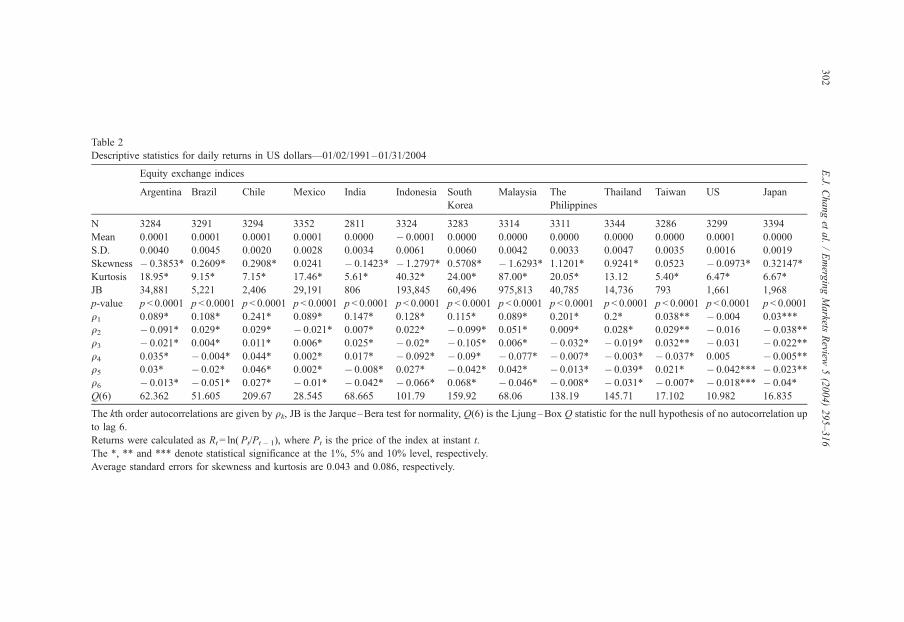
Table 2

Descriptive statistics for daily returns in US dollars—01/02/1991–01/31/2004

Equity exchange indices

Argentina Brazil Chile Mexico India Indonesia South

Korea

Malaysia The

Philippines

Thailand Taiwan US Japan

N 3284 3291 3294 3352 2811 3324 3283 3314 3311 3344 3286 3299 3394

Mean 0.0001 0.0001 0.0001 0.0001 0.0000 � 0.0001 0.0000 0.0000 0.0000 0.0000 0.0000 0.0001 0.0000

S.D. 0.0040 0.0045 0.0020 0.0028 0.0034 0.0061 0.0060 0.0042 0.0033 0.0047 0.0035 0.0016 0.0019

Skewness � 0.3853* 0.2609* 0.2908* 0.0241 � 0.1423* � 1.2797* 0.5708* � 1.6293* 1.1201* 0.9241* 0.0523 � 0.0973* 0.32147*

Kurtosis 18.95* 9.15* 7.15* 17.46* 5.61* 40.32* 24.00* 87.00* 20.05* 13.12 5.40* 6.47* 6.67*

JB 34,881 5,221 2,406 29,191 806 193,845 60,496 975,813 40,785 14,736 793 1,661 1,968

p-value p< 0.0001 p< 0.0001 p< 0.0001 p< 0.0001 p< 0.0001 p< 0.0001 p< 0.0001 p< 0.0001 p< 0.0001 p< 0.0001 p< 0.0001 p< 0.0001 p< 0.0001

q1 0.089* 0.108* 0.241* 0.089* 0.147* 0.128* 0.115* 0.089* 0.201* 0.2* 0.038** � 0.004 0.03***

q2 � 0.091* 0.029* 0.029* � 0.021* 0.007* 0.022* � 0.099* 0.051* 0.009* 0.028* 0.029** � 0.016 � 0.038**

q3 � 0.021* 0.004* 0.011* 0.006* 0.025* � 0.02* � 0.105* 0.006* � 0.032* � 0.019* 0.032** � 0.031 � 0.022**

q4 0.035* � 0.004* 0.044* 0.002* 0.017* � 0.092* � 0.09* � 0.077* � 0.007* � 0.003* � 0.037* 0.005 � 0.005**

q5 0.03* � 0.02* 0.046* 0.002* � 0.008* 0.027* � 0.042* 0.042* � 0.013* � 0.039* 0.021* � 0.042*** � 0.023**

q6 � 0.013* � 0.051* 0.027* � 0.01* � 0.042* � 0.066* 0.068* � 0.046* � 0.008* � 0.031* � 0.007* � 0.018*** � 0.04*

Q(6) 62.362 51.605 209.67 28.545 68.665 101.79 159.92 68.06 138.19 145.71 17.102 10.982 16.835

The kth order autocorrelations are given by qk, JB is the Jarque–Bera test for normality, Q(6) is the Ljung–Box Q statistic for the null hypothesis of no autocorrelation up

to lag 6.

Returns were calculated as Rt= ln( Pt/Pt� 1), where Pt is the price of the index at instant t.

The *, ** and *** denote statistical significance at the 1%, 5% and 10% level, respectively.

Average standard errors for skewness and kurtosis are 0.043 and 0.086, respectively.

E.J.

Changet

al./Emerg

ingMarkets

Review

5(2004)295–316

302

Table 3

VR of equity returns in US dollars (daily data from January 1991 to January 2004)

VR( q) Investment horizon ( q)

2 4 8 16 32 64 128 256 512 Wald

Argentina 1.093 1.038 1.045 1.135 1.263 1.336 1.459 1.794 1.481 34.919

p-value 0.014 0.244 0.278 0.127 0.066 0.064 0.051 0.022 0.087 (0.008)

Brazil 1.113 1.183 1.163 1.210 1.280 1.228 1.134 1.090 1.010 29.198

p-value 0.000 0.000 0.024 0.032 0.037 0.119 0.231 0.278 0.293 (0.003)

Chile 1.241 1.396 1.560 1.809 2.148 2.165 2.268 2.650 2.640 134.255

p-value 0.000 0.000 0.000 0.000 0.000 0.000 0.002 0.001 0.004 (0.000)

Mexico 1.091 1.124 1.137 1.241 1.389 1.519 1.444 1.335 0.984 16.002

p-value 0.010 0.022 0.054 0.025 0.017 0.025 0.071 0.124 0.290 (0.094)

India 1.150 1.250 1.302 1.419 1.474 1.628 1.648 1.686 1.186 49.826

p-value 0.000 0.000 0.000 0.001 0.004 0.010 0.017 0.037 0.177 (0.002)

Indonesia 1.143 1.237 1.168 1.253 1.498 1.572 1.647 1.953 1.382 42.559

p-value 0.001 0.002 0.061 0.061 0.018 0.040 0.053 0.037 0.128 (0.006)

South Korea 1.093 1.026 0.895 0.954 1.050 1.111 1.179 1.381 1.030 29.592

p-value 0.007 0.316 0.120 0.404 0.326 0.258 0.214 0.138 0.282 (0.021)

Malaysia 1.101 1.201 1.186 1.166 1.189 1.469 1.683 1.944 1.650 22.237

p-value 0.013 0.008 0.047 0.097 0.149 0.065 0.049 0.037 0.090 (0.049)

The Philippines 1.204 1.312 1.334 1.510 1.758 2.042 2.087 2.217 2.429 72.882

p-value 0.000 0.000 0.000 0.000 0.000 0.000 0.000 0.003 0.004 (0.000)

Thailand 1.187 1.295 1.309 1.441 1.587 1.714 1.604 1.986 2.267 75.116

p-value 0.000 0.000 0.001 0.003 0.002 0.006 0.021 0.016 0.016 (0.000)

Taiwan 1.036 1.099 1.115 1.163 1.236 1.298 1.225 1.138 0.652 14.954

p-value 0.048 0.016 0.047 0.050 0.041 0.055 0.152 0.223 0.347 (0.107)

US 0.994 0.957 0.877 0.836 0.799 0.749 0.801 1.051 1.432 9.559

p-value 0.393 0.154 0.034 0.047 0.085 0.109 0.303 0.304 0.098 (0.355)

Japan 1.029 0.996 0.924 0.912 0.937 0.976 1.062 1.129 0.985 11.616

p-value 0.078 0.485 0.121 0.186 0.336 0.499 0.313 0.242 0.326 (0.225)

Row 1 reports the VR( q) and row 2 reports one-sided p-value. The final column shows the Wald statistic and the

bootstrapped p-value is given in parenthesis.


investigate the source of this predictability. In the next subsection we will perform tests to

check whether we are able to earn positive profits from technical trading rules through the

use of bootstrap techniques as in Brock et al. (1992) and Ratner and Leal (1999).

5.2. Technical trading rules

Tables 4 and 5 present results for the 1_50, 1_150, 5_150, 1_200 and 2_200 VMA rules.

A rule is significant when it satisfies two conditions: a p-value less than 0.10 and a positive

excess return. For emerging markets we have 11 countries and 5 rules. In Table 4, 16 out of

these 55 rules are statistically significant at least at the 10% level. If we only consider rules

that are statistically significant at the 5% level, there are only 6 rules with explanatory power.

From Table 5 we can see that if we average returns we find an average annualized

excess return of � 3.35% for emerging markets with the VMA rules.

In Tables 6 and 7, we present results for the TRB trading rules. From Table 6 we see

that out of the 55 rules we have nine significant rules. However, most of these significant

strategies are concentrated in trading rules that use a greater number of observations. Rules

Table 4

Test results from VMA rules

Argentina Brazil Chile Mexico India Indonesia South Korea Malaysia The Philippines Thailand Taiwan US Japan

1_50

Buy 29.79 43.00 25.46 22.40 26.26 145.80 � 0.68 11.24 14.98 29.10 21.40 2.16 2.22

Sell 1.23 � 15.92 � 2.59 � 11.41 � 7.01 � 8.18 � 13.45 � 10.30 � 13.17 � 9.53 � 8.97 � 2.87 � 6.47

p-value 0.23 0.02 0.06*** 0.04 0.02 0.09*** 0.36 0.06 0.00 0.00 0.02 0.75 0.19

1_150

Buy 26.19 23.53 14.20 9.46 26.37 107.97 21.21 24.42 15.16 13.85 22.66 9.05 8.35

Sell � 5.03 � 1.13 � 2.72 � 5.34 � 4.26 � 3.09 � 7.09 � 2.90 � 8.27 � 2.98 � 6.86 � 1.58 � 1.49

p-value 0.15 0.47 0.35 0.45 0.05*** 0.19 0.09 0.02** 0.02** 0.14 0.03** 0.45 0.16

5_150

Buy 30.83 23.15 14.53 9.02 29.71 117.05 28.28 27.17 13.90 12.58 27.85 11.34 9.06

Sell � 2.62 � 4.13 � 3.29 � 0.25 � 0.63 � 6.17 � 1.14 � 2.11 � 4.53 � 3.37 � 1.44 � 3.34 � 2.59

p-value 0.12 0.39 0.26 0.64 0.04** 0.17 0.09*** 0.01** 0.05*** 0.17 0.04** 0.20 0.11

1_200

Buy 9.81 20.29 11.59 0.68 18.19 124.91 17.69 20.06 10.51 14.52 21.98 13.13 6.24

Sell � 3.90 � 5.62 � 3.96 � 5.67 � 6.94 � 5.78 � 4.20 � 4.00 � 7.92 � 5.83 � 2.67 1.39 � 1.11

p-value 0.52 0.46 0.44 0.72 0.11 0.16 0.19 0.05*** 0.05*** 0.06 0.07*** 0.44 0.22

2_200

Buy 10.02 19.68 10.93 4.00 16.48 118.98 22.16 21.06 10.12 10.85 23.21 14.16 7.76

Sell � 3.26 � 2.34 � 2.53 � 9.46 � 5.87 � 3.47 � 3.41 � 0.53 � 4.24 � 1.66 � 3.04 � 1.62 � 1.24

p-value 0.52 0.53 0.49 0.47 0.14 0.18 0.12 0.06*** 0.10 0.27 0.05*** 0.15 0.17

The first and second rows present annualized returns conditional on buy and sell signals. The third row presents the bootstrapped p-value for the Buy–Sell statistic. If the

Buy–Sell statistic is significant at the 5% level then its value is greater than the Buy–Sell statistic for more than 95% of the bootstrapped series. We only consider as

statistically significant rules that have Buy–Sell p-values less than 10% and also positive excess return (see Table 5).


The Buy–Sell statistic is given by:


s=ns

q

E.J.

Changet

al./Emerg

ingMarkets

Review

5(2004)295–316

304

Table 5

Test results from VMA rules


1_50

N(Buy) 1806 1836 1698 1946 1346 1642 1607 1767 1541 1637 1562 2161 1490

N(Sell) 1428 1405 1546 1356 1415 1632 1626 1497 1720 1657 1674 1088 1854

Excess Return � 0.95 � 8.97 1.37* � 7.53 � 1.00 14.52* � 16.68 � 4.67 � 2.34 � 18.43 � 1.44 � 9.15 � 3.02

p-value 0.03 0.11 0.00 0.04 0.01 0.00 0.36 0.04 0.01 0.53 0.02 0.68 0.28

1_150

N(Buy) 1700 1834 1664 1875 1383 1549 1552 1745 1660 1571 1507 2268 1489

N(Sell) 1434 1307 1480 1327 1278 1625 1581 1419 1501 1623 1629 881 1755

Excess Return � 2.42 � 6.71 0.63 � 8.18 1.28** 4.19 � 4.44 4.42** 2.92** � 22.86 0.52** � 4.23 2.00

p-value 0.09 0.14 0.01 0.23 0.03 0.12 0.13 0.01 0.02 0.67 0.06 0.27 0.11

5_150

N(Buy) 1714 1840 1676 1876 1389 1539 1542 1741 1658 1576 1503 2283 1482

N(Sell) 1420 1301 1468 1326 1272 1635 1591 1423 1503 1618 1633 866 1762

Excess Return 0.80*** � 8.01 � 0.69 � 6.39 4.58** 4.37 1.32*** 6.05** 4.27*** � 23.43 5.56** � 3.20 1.66

p-value 0.06 0.24 0.04 0.26 0.03 0.16 0.08 0.02 0.05 0.69 0.03 0.25 0.18

1_200

N(Buy) 1578 1776 1563 1921 1281 1545 1509 1781 1599 1677 1518 2253 1461

N(Sell) 1506 1315 1531 1231 1330 1579 1574 1333 1512 1467 1568 846 1733

Excess Return � 2.00 � 11.78 � 1.58 � 11.71 � 2.84 3.04 � 4.74 0.90*** 0.93*** � 24.17 2.30*** � 0.77 1.87

p-value 0.09 0.40 0.03 0.55 0.14 0.16 0.19 0.06 0.05 0.69 0.06 0.03 0.13

2_200

N(Buy) 1582 1777 1565 1911 1290 1543 1505 1782 1599 1674 1520 2248 1456

N(Sell) 1502 1314 1529 1241 1321 1581 1578 1332 1512 1470 1566 851 1738

Excess Return � 1.57 � 10.74 � 1.15 � 11.41 � 2.90 2.88 � 2.61 2.94** 2.68*** � 23.96 2.62*** � 0.96 2.45

p-value 0.09 0.39 0.04 0.63 0.21 0.19 0.17 0.04 0.05 0.69 0.07 0.06 0.13

The first and second rows present the number of buy (N(Buy)) and sell signals (N(Sell)) generated by a specific rule. The third row presents the annualized excess return for the strategy

(considering transaction costs and the buy and hold strategy). If the excess return is greater than 95% of the excess return of the bootstrapped series, then it is significant at the 5% level.


E.J.

Changet

al./Emerg

ingMarkets

Review

5(2004)295–316

305

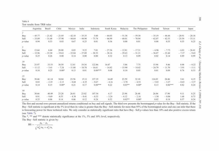
Table 6

Test results from TRB rules


2

Buy � 45.77 � 21.42 � 21.05 � 42.18 � 35.35 5.60 � 64.03 � 51.38 � 59.30 � 35.19 � 44.44 � 20.91 � 28.18

Sell � 33.89 � 31.68 � 37.90 � 44.64 � 44.90 � 73.74 � 66.99 � 68.01 � 70.94 � 62.07 � 42.53 � 25.54 � 33.11

p-value 0.94 0.53 0.03 0.67 0.25 0.01 0.36 0.00 0.01 0.00 0.55 0.55 0.25

5

Buy 13.64 6.64 28.00 0.03 9.22 7.01 � 27.36 � 12.81 � 17.31 � 6.96 � 7.73 � 6.81 � 26.41

Sell � 12.96 � 22.30 � 19.63 � 22.84 � 27.89 � 38.53 � 38.16 � 29.63 � 31.21 � 36.07 � 22.44 � 7.37 � 9.43

p-value 0.25 0.26 0.00 0.14 0.00 0.00 0.32 0.13 0.09 0.02 0.14 0.89 0.99

10

Buy 25.97 33.53 38.59 12.81 19.34 122.86 14.47 5.86 7.75 15.94 9.46 0.98 � 0.22

Sell � 11.12 � 3.41 � 7.24 � 11.88 � 10.78 � 16.61 � 14.82 � 15.90 � 14.42 � 24.79 � 11.70 � 3.91 � 5.11

p-value 0.10 0.25 0.00* 0.13 0.01 0.09*** 0.08 0.10 0.05 0.01 0.09 0.76 0.33

25

Buy 38.46 41.14 34.84 23.56 15.11 137.19 16.49 23.59 32.10 116.03 24.46 3.61 4.15

Sell 0.83 � 2.19 � 2.13 � 0.68 � 4.35 � 9.67 �4.16 � 3.70 � 4.53 � 5.83 � 3.27 � 0.65 � 3.37

p-value 0.14 0.15 0.00* 0.21 0.17 0.08*** 0.22 0.03** 0.00* 0.13 0.06*** 0.82 0.24

50

Buy 30.66 40.49 23.28 26.81 23.02 107.54 4.17 23.96 26.48 26.06 17.90 9.11 8.25

Sell 0.91 � 9.69 0.55 � 4.38 � 0.41 � 0.33 � 3.24 � 4.12 � 2.16 � 1.50 � 0.06 1.68 0.73

p-value 0.25 0.06 0.14 0.06 0.12 0.24 0.52 0.02** 0.00* 0.02 0.18 0.57 0.24

The first and second rows present annualized returns conditional on buy and sell signals. The third row presents the bootstrapped p-value for the Buy–Sell statistic. If the

Buy–Sell statistic is significant at the 5% level then its value is greater than the Buy–Sell statistic for more than 95% of the bootstrapped series and one can infer that there

is forecasting power for these technical rules. We only consider as statistically significant rules that have Buy–Sell p-values less than 10% and also positive excess return

(see Table 7).

The *, ** and *** denote statistically significance at the 1%, 5% and 10% level, respectively.

The Buy–Sell statistic is given by:


s=ns

q

E.J.

Changet

al./Emerg

ingMarkets

Review

5(2004)295–316

306

Table 7

Test results from TRB rules


2

N(Buy) 1687 1712 1650 1733 1444 1663 1609 1652 1646 1630 1586 1715 1648

N(Sell) 1595 1577 1642 1617 1365 1659 1672 1660 1663 1712 1698 1582 1744

Excess Return � 50.30 � 43.06 � 37.81 � 51.70 � 44.77 � 59.72 � 68.92 � 63.18 � 67.16 � 63.80 � 47.31 � 31.24 � 31.55

p-value 0.78 0.06 0.00 0.03 0.00 0.00 0.07 0.00 0.00 0.65 0.02 0.99 0.80

5

N(Buy) 1702 1823 1697 1777 1466 1612 1587 1710 1645 1622 1672 1867 1572

N(Sell) 1577 1463 1592 1570 1340 1707 1691 1599 1661 1717 1609 1427 1817

Excess Return � 17.04 � 28.18 � 8.90 � 24.61 � 17.53 � 38.66 � 39.89 � 26.75 � 27.83 � 43.62 � 21.42 � 16.96 � 19.01

p-value 0.13 0.74 0.00 0.39 0.06 0.65 0.88 0.13 0.07 0.78 0.45 0.96 0.98

10

N(Buy) 1712 1788 1703 1780 1431 1660 1596 1699 1601 1708 1662 1874 1607

N(Sell) 1562 1493 1581 1562 1370 1654 1677 1605 1700 1626 1614 1415 1777

Excess Return � 11.54 � 10.91 1.59* � 14.79 � 4.33 3.74** � 12.07 � 11.92 � 8.30 � 31.24 � 9.98 � 11.73 � 4.19

p-value 0.27 0.17 0.00 0.36 0.03 0.02 0.12 0.14 0.02 0.68 0.29 0.91 0.38

25

N(Buy) 1828 1815 1676 1903 1347 1664 1653 1777 1619 1683 1548 1979 1549

N(Sell) 1431 1451 1593 1424 1439 1635 1605 1512 1667 1636 1713 1295 1820

Excess Return 0.30*** � 2.98 3.86* � 3.87 � 3.36 11.61*** � 5.17 3.13** 9.14** 7.20*** 1.52*** � 8.23 � 0.81

p-value 0.06 0.09 0.00 0.10 0.21 0.05 0.22 0.02 0.01 0.06 0.08 0.84 0.31

50

N(Buy) 1876 1971 1664 1952 1303 1545 1613 1726 1550 1578 1549 2237 1419

N(Sell) 1358 1270 1580 1350 1458 1729 1620 1538 1711 1716 1687 1012 1925

Excess Return � 0.16 � 5.32 1.75** � 2.52 0.91 7.21 � 9.75 3.89*** 8.87** � 16.23 1.92 � 3.46 3.51

p-value 0.11 0.17 0.01 0.10 0.11 0.13 0.63 0.05 0.01 0.63 0.12 0.26 0.12

The first and second rows present the number of buy (N(Buy)) and sell signals (N(Sell)) generated by a specific rule. The third row presents the annualized excess return

for the strategy (considering transaction costs and the buy and hold strategy). If the excess return is greater than 95% of the excess return of the bootstrapped series, then it

is significant at the 5% level.


E.J.

Changet

al./Emerg

ingMarkets

Review

5(2004)295–316

307


with 2 and 5 days are hardly significant and, as we can see in Table 7, most of them have a

negative excess return.

In Table 7, we present the number of buy and sell signals and the excess returns of TRB

rules net of trading costs and a buy and hold strategy. This excess return is on average

� 17.99% for TRB rules.

We can see from Tables 4 and 6 that for emerging markets all VMA trading rules have

returns conditional on buy signals greater than returns conditional on sell signals, while the

same holds true for 53 of the TRB trading rules. This suggests that these rules have

forecast power for price movements in these countries.

An interesting finding is that for the US and Japan we have the same qualitative results:

9 out of 10 rules generate returns conditional on buy signals greater than from sell signals

for TRB rules and all VMA rules share this characteristic. However, even if these rules

have forecasting power they are not able to produce significant excess returns when

compared to a buy and hold strategy and when faced with transaction costs.

From Tables 5 and 7 we see that the number of buy signals is higher than the number of

sell signals for all countries from Latin America, Malaysia and the US, which indicates an

upward trend for this group of countries and a downward trend for the remainder group of

countries as pointed out by Hudson et al. (1996).

Empirical results suggest that although there seems to be evidence of predictability,

which is in line with Harvey (1995) and Ferson and Harvey (1991, 1993), it is difficult to

exploit this predictability and the benchmark technical rules proposed in Ratner and Leal

(1999) do not provide investors with a high return as one would expect after taking into

account transaction costs and a buy and hold strategy. Equity returns for the US seem to be

less predictable than returns for the rest of the countries in the sample. Furthermore, it

seems that equity returns for countries from Latin America possess less predictive power

than those from Asian equity markets.

An interesting question is to ask why these rules are so appealing to investors. One

could guess that these technical rules may generate profits in good market conditions.

Therefore, we test whether these results hold in both bear and bull subperiods. In Table

8 we define bull and bear sample subperiods for all indices to test whether the excess

return from technical trading rules behave differently within these subperiods.16

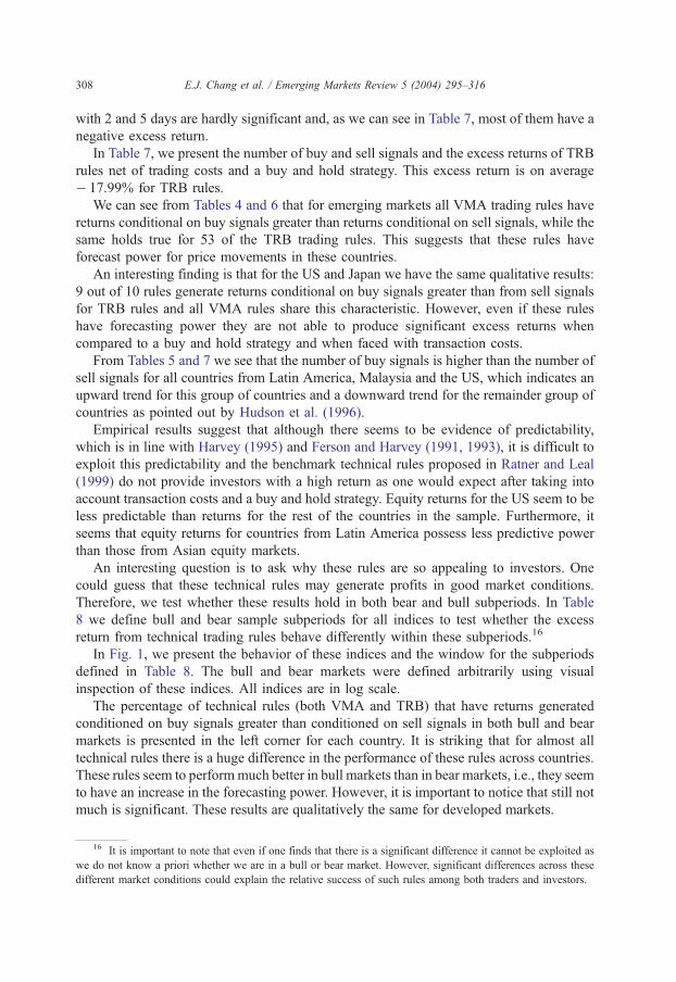
In Fig. 1, we present the behavior of these indices and the window for the subperiods

defined in Table 8. The bull and bear markets were defined arbitrarily using visual

inspection of these indices. All indices are in log scale.

The percentage of technical rules (both VMA and TRB) that have returns generated

conditioned on buy signals greater than conditioned on sell signals in both bull and bear

markets is presented in the left corner for each country. It is striking that for almost all

technical rules there is a huge difference in the performance of these rules across countries.

These rules seem to performmuch better in bull markets than in bear markets, i.e., they seem

to have an increase in the forecasting power. However, it is important to notice that still not

much is significant. These results are qualitatively the same for developed markets.

16 It is important to note that even if one finds that there is a significant difference it cannot be exploited as

we do not know a priori whether we are in a bull or bear market. However, significant differences across these

different market conditions could explain the relative success of such rules among both traders and investors.

Table 8

Bull and bear subperiods

Bull subperiod Bear subperiod

Argentina 02/24/95 09/04/97 02/17/00 11/05/01

Brazil 02/20/95 07/07/97 07/08/97 01/19/99

Chile 05/10/93 11/07/94 06/04/97 09/16/98

Mexico 03/21/95 09/10/97 02/22/94 03/20/95

India 11/20/98 02/18/00 02/21/00 07/23/01

Indonesia 02/04/93 02/03/94 07/30/97 09/28/98

South Korea 08/05/98 12/13/99 12/14/99 08/30/01

Malaysia 10/01/98 03/02/00 02/11/97 09/30/98

The Philippines 01/02/91 11/08/93 02/13/97 10/08/98

Thailand 12/04/91 12/16/93 06/20/96 12/29/97

Taiwan 11/24/95 07/31/97 05/01/00 09/13/01

US 04/16/97 04/12/00 04/13/00 11/11/02

Japan 08/17/98 01/27/00 01/28/00 02/11/02

The bull and bear subperiods have been defined a priori from visual inspection. The beginning and ending for

each one of these subperiods are presented in the first and second columns, respectively.


From the results presented so far, it seems that although technical trading rules have some

forecasting power they seem to performmuch better in bull rather than in bearmarkets and that

potential profits seem to be much higher in emerging markets than in developed markets.

The next step in our testing strategy is to analyze the behavior of different combinations

of the VMA and the TRB rules. We allow the short-term moving average to range from 1

to 10 days while the long-term moving average ranges from 50 to 200 days. By studying

all these combinations we have 1510 trading rules. For the TRB we analyze rules that use

2 to 50 days (49 technical rules).

In Fig. 1, we also present the results for all trading rules inside the graph box for each

country. In the first line we show the proportion of the 1559 trading rules that have had a

significant buy–sell statistic. Furthermore, we have analyzed two subperiods; we study

these rules from January 1991 to December 1997 and from January 1998 to January 2004.

Therefore, we have used the Asian crisis to split the sample.

We can see that for the US none of these rules are significant and that predictability is

much greater for emerging economies than for the US. For Malaysia and the Philippines,

the proportion of rules that possess forecasting power is certainly high.

The average proportion for the full sample of significant buy–sell statistics is 30.29%

for emerging markets, 7.02% for Latin America and is 43.59% for Asian economies. The

numbers are 3.59% and 15.65% for Latin America during the first and second subperiods,

respectively, and 27.84% and 20.27% for Asian economies. These results suggest that the

degree of forecasting power in Asian economies has decreased over time while those of

Latin America have increased.17

We also present, in Table 9, the best rules for the full sample and for the same

subperiods. We fix the best rule for the first subperiod and test its performance in the latter

17 It is important to notice that some of these Asian economies changed from a currency peg exchange rate

regime to a floating exchange rate regime. As we are employing returns denominated in US dollars the exchange

rate component could lower the predictive power.

Fig. 1. The indices are presented in log levels with bull and bear subperiods chosen by visual inspection. In the left corner we present the proportion of rules that have

returns conditional on buy signals greater than returns conditional on sell signals. We also present the same information inside the figures for the full sample and also for

the January 1991–December 1997 and January 1998–January 2004 subperiods.

E.J.

Changet

al./Emerg

ingMarkets

Review

5(2004)295–316

310

Fig.1(continued

).


Fig. 1 (continued ).


subperiod. The best rule is defined as the one that generates the highest excess return

(regardless of its statistical significance). In the first row we present the name of the rules

and in the second and third rows we show the excess return and the p-value for the buy–

sell statistic. For example, TRB_17 stands for a TRB with 17 days and 4_57 a VMAwith a

short moving average of 4 days and a long-term moving average of 57 days.

From Table 9 we can see that only for Chile, India, Indonesia and the Philippines we

have significant rules for both subperiods. These results are in line with previous findings.

Although technical rules possess some forecasting power not much is statistically

significant and this is robust when searching through the best rules available from

different combinations.

6. Concluding remarks

From multivariate VR statistics evidence suggests that emerging equity market indices

do not resemble a random walk. On the other hand, for the US and Japan we are not able to

reject the RWH using the same methodology, which is in line with the findings of Chow

and Denning (1993) for the US using another multivariate VR statistic. These findings

suggest that there is predictability in emerging equity returns.

Our empirical results for trading rules show some evidence of predictability, which is in

line with those found with the use of VR. However, the empirical results suggest that, in

general, trading rules do not generate statistically significant profits after taking into

account both transaction costs and a buy and hold strategy. Furthermore, on average TRB

rules tend to perform worse than moving average trading rules.

The technical trading rules employed in this study do not seem to have forecasting

power for the US. This could be due to the immense literature that has focused on this

Table 9

First and second best rules from 1559 trading rules (1510 VMA rules and 49 TRB rules) for the full sample and subperiods


1st Best Rule

Full sample 7_190 TRB_34 TRB_17 TRB_42 7_156 5_51 10_175 10_95 5_63 TRB_25 10_137 9_196 5_69

Return 6.57 0.48 7.54 1.19 6.14 20.62 2.11 9.48 13.25 7.20 7.94 0.36 4.98

Buy–Sell 0.34 0.05*** 0.00* 0.04** 0.04** 0.06*** 0.06*** 0.00* 0.00* 0.13 0.02** 0.12 0.07***

1st subperiod 3_149 6_124 TRB_28 9_61 8_152 1_79 7_144 10_57 TRB_49 TRB_30 7_107 9_197 10_60

Return � 2.10 � 8.76 5.27 4.71 9.17 31.13 21.70 14.61 6.83 13.20 6.99 � 2.33 8.01

Buy–Sell 0.27 0.81 0.04** 0.03** 0.06*** 0.09*** 0.10 0.00* 0.02** 0.27 0.11 0.92 0.15

2nd subperiod 3_149 6_124 TRB_28 9_61 8_152 1_79 7_144 10_57 TRB_49 TRB_30 7_107 9_197 10_60

Return 7.34 4.73 4.55 � 6.91 1.81 1.54 � 10.46 � 2.96 16.71 6.10 1.40 3.90 0.82

Buy–Sell 0.16 0.08*** 0.02** 0.26 0.08*** 0.01** 0.34 0.53 0.09*** 0.03** 0.19 0.09*** 0.18

2nd Best Rule

Full sample 7_189 5_70 TRB_20 TRB_43 7_155 5_50 6_171 10_94 5_62 TRB_23 10_140 9_194 5_70

Return 6.42 � 0.20 7.00 0.64 6.14 20.40 1.95 9.23 12.64 6.91 7.88 0.27 4.88

Buy–Sell 0.30 0.11 0.00* 0.03** 0.03** 0.06*** 0.07*** 0.00* 0.00* 0.16 0.02** 0.18 0.07***

1st subperiod 1_108 6_123 3_54 10_62 7_152 1_81 7_145 7_53 TRB_50 TRB_29 10_110 9_198 5_69

Return � 2.14 � 8.87 4.32 4.59 9.07 30.81 21.46 14.57 6.64 11.86 6.96 � 2.33 7.86

Buy–Sell 0.57 0.84 0.05*** 0.06*** 0.07*** 0.09*** 0.10 0.00* 0.01** 0.27 0.11 0.93 0.13

2nd subperiod 1_108 6_123 3_54 10_62 7_152 1_81 7_145 7_53 TRB_50 TRB_29 10_110 9_198 5_69

Return � 1.96 4.44 0.46 � 8.09 1.52 3.89 � 11.46 � 1.56 14.59 5.07 � 0.44 4.71 4.10

Buy–Sell 0.44 0.06*** 0.08*** 0.25 0.04** 0.07*** 0.34 0.14 0.16 0.10 0.31 0.09*** 0.10

We have analyzed 1559 trading rules using different combinations of VMA and TRB rules. We present the 1st and 2nd best rules for the full sample. We also divide the

sample in two subperiods, from January 1991 to December 1997 and from January 1998 to January 2004. We test whether the 1st and 2nd best rules found for the 1st

subperiod remain significant in the 2nd subperiod. Comparing the actual Buy–Sell statistic with the Buy–Sell statistics of the bootstrapped series we assess the

significance of the Buy–Sell statistics.

The *, ** and *** denote statistical significance at the 1%, 5% and 10% level. Returns are annualized excess returns net of trading costs and a buy and hold strategy.

TRB_ j stands for a Trading Range Break strategy (TRB) with j days and i_ j for a variable moving average (VMA) with short and long moving averages, of i and j days,

respectively.

E.J.

Changet

al./Emerg

ingMarkets

Review

5(2004)295–316

314


market for the past decade. If traders and analysts read financial papers, since the literature

has pointed out that these trading rules have significant forecasting power, the widespread

use of these rules could have wiped out the potential for gains from them.

In Chile’s case, Parisi and Vasquez (2000) find evidence providing strong support for

technical strategies. Our paper suggests that these opportunities seem to have been

decreased substantially. Nonetheless, in this paper we have used a more recent data set

and compared the returns for trading rules with a buy and hold strategy, which could

explain the difference in the results. With regard to Ratner and Leal’s (1999) results, which

point out that Taiwan, Thailand, and Mexico emerged as markets with trading opportu-

nities, this paper has found that evidence for Mexico has disappeared while there is

renewed evidence for other Asian emerging markets. In general, trading rules seem to

perform better for both Malaysia and the Philippines.

When we investigate a combination of 1559 rules we find that there is some forecasting

power, but not much is significant. These results suggest that the usual trading rules that

have been used in most of the literature stemming from Brock et al. (1992) do not possess

forecasting power for these markets but other rules could have to some extent. This could

be due to the fact that these rules are widely known and have been broadly employed,

which would minimize the potential gains that one could obtain from them.

The general conclusion from the studies of Brock et al. (1992) and Hudson et al. (1996)

is that technical trading rules have predictive ability if sufficiently long series of data are

considered. In contrast to their findings, our empirical results suggest that for emerging

markets, if we take into account both transaction costs and a buy and hold strategy we find

some evidence of predictability using technical trading rules but not much is statistically

significant.

The results in this paper indicate that it is worthwhile to investigate more elaborate rules

since simple technical trading rules can yield positive excess returns even when

accounting for transaction costs and a buy and hold strategy. An interesting alternative

would be to test for the forecasting power of nonlinear rules.

Acknowledgements

The authors gratefully acknowledge Donald Piantto and Nathalia Souza for helpful

comments. We are especially indebted to an anonymous referee whose comments led to a

considerable improvement of the paper. We also thank participants at the 3rd Brazilian

Finance Association Meeting and XXV Brazilian Econometric Society Meeting where a

preliminary version of the paper was presented.

References

Ayadi, O.F., Pyun, C.S., 1994. An application of the variance ratio test to Korean securities market. Journal of

Banking and Finance 18, 643–658.

Bekaert, G., Erb, C.B., Harvey, C.R., Viskantas, T.E., 1998. Distributional characteristics of emerging markets

returns and asset allocation. Journal of Portfolio Management, 102–116 (Winter volume).

Bessembinder, H., Chan, K., 1995. The profitability of technical trading rules in the Asian stock markets. Pacific-

Basin Finance Journal 3, 257–284.


Blasco, N., Rio, C.D., Santamarıa, R., 1997. The random walk hypothesis in the Spanish stock market:

1980–1992. Journal of Business Finance and Accounting 24, 667–683.

Brock, W., Lakonishok, J., LeBaron, B., 1992. Simple technical trading rules and the stochastic properties of

stock returns. Journal of Finance 47, 1731–1764.

Ceccheti, S.G., Lam, P.-S., 1994. Variance-ratio tests: small-sample properties with an application to international

output data. Journal of Business & Economic Statistics 12, 177–186.

Chow, K.V., Denning, K.C., 1993. A simple multiple variance ratio test. Journal of Econometrics 58, 385–401.

Darrat, A.F., Zhong, M., 2000. On testing the random-walk hypothesis: a model comparison approach. The

Financial Review 35, 105–124.

Fernandez-Rodriguez, F., Gonzalez-Martel, C., Sosvilla-Rivero, S., 2000. On the profitability of technical

trading rules based on artificial neural networks: evidence from the Madrid stock market. Economics Letters

69, 89–94.

Ferson, W.E., Harvey, C.R., 1991. Sources of predictability in portfolio returns. Financial Analysts Journal,

49–56 (May/June volume).

Ferson, W.E., Harvey, C.R., 1993. Explaining the predictability of asset returns. Research in Finance 11, 65–106.

Frennberg, P., Hansson, B., 1993. Testing the random walk hypothesis on Swedish stock prices: 1919–1990.

Journal of Banking and Finance 17, 175–191.

Genc�ay, R., 1998. The predictability of security returns with simple technical trading rules. Journal of Empirical

Finance 5, 347–359.

Grieb, T., Reyes, M.G., 1999. Random walk tests for Latin American equity indexes and individual firms. The

Journal of Financial Research 22, 371–383.

Gunesekarage, A., Power, D.M., 2001. The profitability of moving average trading rules in South Asian stock

markets. Emerging Markets Review 2, 17–33.

Harvey, C.R., 1995. Predictable risk and returns in emerging markets. The Review of Financial Studies 8,

773–816.

Harvey, C.R., Travers, K.E., Costa, M.J., 2000. Forecasting emerging markets returns using neural networks.

Emerging Markets Quarterly 4, 43–54.

Huang, B.-N., 1995. Do Asian stock market prices follow random walks? Evidence from the variance ratio test.

Applied Financial Economics 5, 251–256.

Hudson, R., Dempsey, M., Keasey, K., 1996. A note on the weak form efficiency of capital markets: the

application of simple technical trading rules to UK stock prices—1935 to 1994. Journal of Banking and

Finance 20, 1121–1132.

Karamera, D., Ojah, K., Cole, J.A., 1999. Random walks and market efficiency tests: evidence from emerging

equity markets. Review of Quantitative Finance and Accounting 13, 171–188.

Kwon, K.-Y., Kish, R.J., 2002. A comparative study of technical trading strategies and return predictability: an

extension of Brock, Lakonishok, and LeBaron (1992) using NYSE and NASDAQ indices. The Quarterly

Review of Economics and Finance 42, 611–631.

Lo, A.W., MacKinlay, A.C., 1988. Stock market prices do not follow random walks: evidence from a simple

specification test. The Review of Financial Studies 1, 41–66.

Lo, A.W., MacKinlay, A.C., 1989. The size and power of the variance ratio test in finite samples: a Monte Carlo

investigation. Journal of Econometrics 40, 203–238.

Malliaropulos, D., Priestley, R., 1999. Mean reversion in Southeast Asian stock markets. Journal of Empirical

Finance 6, 355–384.

Parisi, F., Vasquez, A., 2000. Simple technical trading rules of stock returns: evidence from 1987 to 1998 in

Chile. Emerging Markets Review 1, 152–164.

Poterba, J., Summers, L., 1988. Mean reversion in stock returns: evidence and implications. Journal of Financial

Economics 22, 27–60.

Ratner, M., Leal, R.P.C., 1999. Tests of technical trading strategies in the emerging equity markets of Latin

America and Asia. Journal of Banking and Finance 23, 1887–1905.

Urrutia, J.L., 1995. Test of random walk and market efficiency for Latin American emerging equity markets. The

Journal of Financial Research 18, 299–309.

Testing for predictability in emerging equity markets

Documents

Transcript of Testing for predictability in emerging equity markets