Value-at-Risk for long and short trading positions:

Evidence from developed and emerging equity markets

by

Panayiotis F. Diamandis1,*

, Anastassios A. Drakos1,

Georgios P. Kouretas1,2

and Leonidas Zarangas3

May 14, 2010

Abstract

The financial crisis of 2007-2009 has questioned the provisions of Basel II agreement

on capital adequacy requirements and the appropriateness of VaR measurement. This

paper reconsiders the use of Value-at-Risk as a measure for potential risk of economic

losses in financial markets by estimating VaR for daily stock returns with the

application of various parametric univariate models that belong to the class of ARCH

models which are based on the skewed Student distribution. We use daily data for

three groups of stock market indices, namely Developed, Southeast Asia and Latin

America. The data covers the period 1987-2009. We conduct our analysis with the

adoption of the methodology suggested by Giot and Laurent (2003). Therefore, we

estimate an APARCH model based on the skewed Student distribution to fully take

into account the fat left and right tails of the returns distribution. The main finding of

our analysis is that the skewed Student APARCH improves considerably the forecasts

of one-day-ahead VaR for long and short trading positions. Additionally, we evaluate

the performance of each model with the calculation of Kupie‟s (1995) Likelihood

Ratio test on the empirical failure test. Moreover, for the case of the skewed Student

APARCH model we compute the expected shortfall and the average multiple of tail

event to risk measure. These two measures help us to further assess the information

we obtained from the estimation of the empirical failure rates.

Keywords: Value-at-Risk, risk management, APARCH models, skewed Student

distribution

JEL Classification: C53, G21; G28

*We have benefited from comments by seminar participants at the Athens University of Economics

and Business, the University of Crete and Philips College. Kouretas acknowledges financial support

from a Marie Curie Transfer of Knowledge Fellowship of the European Community's Sixth Framework

Programme under contract number MTKD-CT-014288, as well as from the Research Committee of the

University of Crete under research grants #2016, #2030 and #2257. We also thank without implicating,

Richard Baillie, Dimitris Georgoutsos, Dimitris Moschos, Lucio Sarno and Elias Tzavalis for numerous

valuable comments and discussions on an earlier draft.

1 Department of Business Administration, Athens University of Economics and Business, GR-10434,

Athens, Greece. 2Centre for International Business and Management, Cambridge Judge Business School, Trumpington

Street, Cambridge CB2 1AG, United Kingdom. 3 Department of Finance and Auditing, Technological Educational Institute of Epirus, 210 Ioanninon

Ave., GR-48100, Preveza, Greece.

*corresponding author: email: kouretas@aueb.gr; telephone, 2108203277, fax: 2108226203.

1

1. Introduction

During the recent years the importance of effective risk management has

become extremely crucial. This is the outcome of several significant factors. First, the

enormous growth of trading activity that has been taking place in the stock markets,

especially those of the emerging economies which, however, led to an increase in

financial uncertainty and increased volatility in the stock returns. Indeed, during the

period 1992-2008 an enormous inflow of portfolio funds to the emerging markets of

Central and Eastern Europe, Southeast Asia and Latin was recorded and this capital

inflow was due to the fact that over this period the mature markets have reached their

limitations with respect to profit opportunities leading portfolio managers and

institutional investors to look for new opportunities in these new markets. Second, the

financial disasters that took place in the 1990s that have led to bankruptcy well-

known financial institutions. These events have put great emphasis for the

development and adoption of accurate measures of market risk by financial

institutions. Financial regulators and supervisory committee of banks have favoured

quantitative risk techniques which can be used for the evaluation of the potential loss

that financial institutions can suffer. Furthermore, given that the nature of these risks

changes over time effective risk management measures must be responsive to news

such as other forecasts as well as to be easy understood even in complicated cases.

This need was further reinforced by a number of financial crises that took

place in the 1980s, 1990s and the 2000s such as the worldwide stock markets collapse

in 1987, the Mexican crisis in 1995, the Asian and Russian financial crises in 1997-

1998, the Orange County default, the Barings Bank, the dot.com bubble and Long

Term Capital Management bankruptcy cases as well as the financial crisis of 2007-

2009 which led several banks to bankruptcy worldwide with Lehman Brothers being

2

the most notable case. Such financial uncertainty has increased the likelihood of

financial institutions to suffer substantial losses as a result of their exposure to

unpredictable market changes. These events have made investors to become more

cautious in their investment decisions while it has also led for the increased need for a

more careful study of price volatility in stock markets. Indeed, recently we observed

an intensive research from academics, financial institutions and regulators of the

banking and financial sectors to better understanding the operation of capital markets

and to develop sophisticated models to analyze market risk.

Basle I and II Agreements has been the main vehicle globally for the set up of

the regulatory framework on financial markets following the dramatic events in

financial markets in the late 1980s and early 1990s. Basle I was introduced in late

1980s and it was based on risk classification of assets with the main purpose to force

banks to provide sufficient capital adequacy against these assets based on their

respective risks. However, it turned out that this attempt to impose capital ratios for

banks had adverse effects since Basle I put a low risk weight on loans by banks to

other financial institutions. In this framework banks were given an incentive to

transfer risky assets of their balance sheets. Regulation arbitrage was further incurred

since Basle I made possible for banks to treat assets that were insured as government

securities with zero risk a feature that was fully exploited by the banks and led to the

huge increase of the market for CDS.

In an attempt to remedy some of the problems created since the

implementation of Basle I Agreement, Basle II was introduced in the 1990s and it was

put in full implementation in 2007. A central feature of the modified Basle II Accord

was to allow banks to develop and use their own internal risk management models

conditional upon that these models were tested under extreme circumstances and

3

properly „backtested” and “stress tested”. Value-at-Risk has become the standard tool

used by financial analysts to measure market risk. VaR is defined as a certain amount

lost on a portfolio of financial assets with a given probability over a fixed number of

days. The confidence level represents „extreme market conditions‟ with a probability

that is usually taken to be 99% or 95%. This implies that in only 1% (5%) of the cases

will lose more than the reported VaR of a specific portfolio. VaR has become a very

popular tool among financial analysts which is widely used because of its simplicity.

Essentially the VaR provides a single number that represents market risk and

therefore it is easily understood.1

During the last decade several approaches in estimating the profit and losses

distribution of portfolio returns have been developed, and a substantial literature of

empirical applications have emerged which provided an overall support for the use of

VaR as the appropriate measure of market risk. A number of these models have

focused on the computation of the VaR on the left tail of the distribution which

corresponds to the negative returns. This implies that it is assumed that portfolio

managers or traders have long trading positions, which means that they bought an

asset at a given price and they are concerned with the case that the price of this asset

falls resulting in losses. More recent approaches dealt with modeling VaR for

portfolios that includes both long and short positions. Therefore, they considered the

modeling and calculation of VaR for portfolio managers who have taken either a long

position (bought an asset) or a short position (sold an asset). As it is well known, in

the former case the risk of a loss occurs when the price of the traded asset falls, while

in the later case the trader will incur a loss when the asset price increases.2 Hence, in

1 See also Bank for International Settlements (1988, 1999a,b,c, 2001).

2 Sharpe et al. (1999) provide a comprehensive analysis of trading strategies.

4

the first case we model the left tail of the distribution of returns and in the second case

we model the right tail of the distribution.

Furthermore, given the stylized fact that the distribution of asset returns is

non-symmetric, Giot and Laurent (2003) using daily data for FTSE100, NASDAQ

and NIKKEI22 have shown that models which rely on a symmetric density

distribution for the error term underperform with respect to skewed density models

when the left and right tails of the distribution of returns must be modeled. This

implies that VaR for portfolio managers or traders who hold both long and short

positions cannot be accurately modeled by the application of the standard normal and

Student distributions. Giot and Laurent (2003) also showed that similar problems arise

when we try to model the distribution with the asymmetric GARCH models which

assume that there is an asymmetry exists between the conditional variance and the

lagged squared error term, (see also El Babsiri and Zakoian, 1999). So and Yu (2006),

Tang and Shieh (2006), McMillan and Speight (2007) and McMillan and

Kambouridis (2009) provided recent evidence on the performance of alternative VaR

models for a large number of stock as well as exchange rate markets. They confirmed

prior evidence that models that take into consideration the asymmetric effects and

long memory features of the data perform better than the models which model the

conditional variance errors to be normally distributed.

The financial crisis of 2007-2009 has raised questions regarding the usefulness

of the regulatory framework underlined by the Basle I and II agreements and it also

questioned the appropriateness of the VaR as the measure to capture extreme cases

like the ones the banking sector and global financial markets experienced over this

turbulent period (See for example, Brunnermeier, 2009; De Grauwe and Welfens,

2009). De Grauwe (2009) argued that the Basle approach to stabilize the banking

5

system has an implicit assumption that financial markets are efficient. Market

efficiency implies that returns are normally distributed. However, it has by now

documented in the finance literature that asset returns are not normally distributed but

they have distributions with fat tails. Therefore, De Grauwe (2009) argued that the

Basle Accords have failed to provide stability in the banking sector since the risks

linked with universal banks are tails risks associated with bubbles and crises. Fat tails

are linked to the occurrence of bubbles and crises and this implies that models based

on normally distributed errors substantially underestimate the probability of large

shocks. These consequences of the financial crisis of 2007-2009 increased the need

for a closer look in modeling the volatility of returns of asset markets and more

importantly to model VaR for portfolios on long and short positions which are mainly

constructed from stocks which are traded in both the mature and emerging markets.

Thus, we focus on the joint behaviour of VaR models for long and short trading

positions.

The aim of this paper is to reconsider the evidence on the forecasting ability of

four competing models in estimating VaR of stock market indices. To conduct our

study to portfolios for long and short positions on daily stock indexes of 21 stock

market indices of developed and emerging markets using data that extends from 1980

to the end of 2009 in order to take into consideration any effects due to the financial

crisis of 2007-2009. In order to account for possible asymmetries in the behavior of

stock returns we applied the univariate Student Asymmetric Power ARCH

(APARCH) model introduced by Ding et al. (1993) which allows to model and

calculate the VaR for portfolios defined on long position (long VaR) and short

position (short VaR). The in-sample and out-of sample performance of this model is

compared with those of the standard parametric Riskmetrics and normal and Student

6

APARCH models. Following Giot and Laurent (2003), So and Yu (2006), Tang and

Shieh (2006), McMillan and Speight (2007) and McMillan and Kambouridis (2009)

we examined the performance of these competing models at the 1% and 5% tails

The main finding of our analysis is that the skewed Student APARCH

improves considerably the forecasts of one-day-ahead VaR for long and short trading

positions. Additionally, we evaluated the performance of each model with the

calculation of Kupie‟s (1995) Likelihood Ratio test on the empirical failure test.

Moreover, for the case of the skewed Student APARCH model we compute the

expected shortfall and the average multiple of tail event to risk measure. These two

measures help us to further assess the information we obtained from the estimation of

the empirical failure rates.

The remainder of the paper is organized as follows. Section 2 describes the

basic concept of VaR and presents the alternative VaR models for modeling financial

return series. In section 3 we report our empirical results and finally section 4

provides our concluding remarks.

2. Value-at-Risk and VaR models

We begin with a brief description of the VaR metric. VaR is the standard

measure of market risk that provides the financial institutions with the information on

the minimum amount that it is expected to lose with a small probability over a

given horizon (which is usually taken to be 1 day). Thus, assuming that the VaR

model is correct, a 1-day vaR at %5 of 10 Euros could tell us that one out of 20

days we could expect to occur a loss exceeding 10 million Euros. Therefore, VaR is

defined as the maximum loss over a given time horizon at a given confidence level.

Coupled with this, the VaR provides information about the required minimum amount

7

of capital required to cover all but a small pre-specified proportion of expected losses.

As we already discussed Basle II Agreement requires that financial institutions

develop their own internal risk management models to assess their market risk. Then,

the true test for these models is provided by “backtesting” which amounts to a

comparison of actual trading losses with the estimated VaR and recording the number

of exceptions (failures). Given, these considerations we define the k -day VaR on day

t is given by:

1)),,(( ktVaRPPP tkt

where P is the stock price on day t .

Assuming a specific distribution of the stock return, we calculate the VaR in

terms of a given percentile of this distribution (Jorion, 2000, Alexander 1003, 2005).

Therefore, if we define q as the percentile of the given distribution of returns,

then VaR can be expressed as:

kt

qPeaktVaR )1(),,(

In obtaining good VaR measures it is crucial therefore to produce accurate

forecasts of the percentiles q . This in turn requires the adoption of alternative

distributional specifications of asset returns that allows for various hypotheses on

conditional volatility.

We followed Giot and Laurent (2003) and provide a brief description of the

four models used in the analysis. The starting point is the definition of the conditional

mean and variance of the disturbance term which is relevant for all alternative VaR

specifications. Therefore, we consider a series of daily returns, ty , with Tt ...1 . In

8

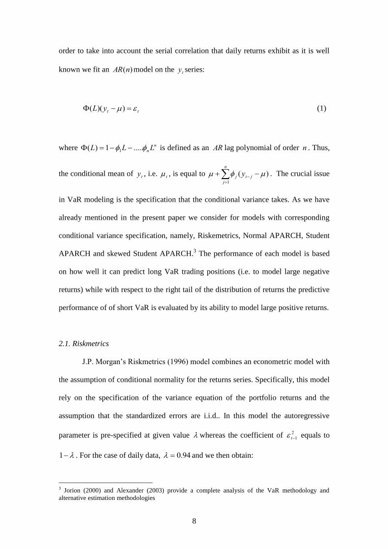
order to take into account the serial correlation that daily returns exhibit as it is well

known we fit an )(nAR model on the ty series:

ttyL ))(( (1)

where n

nLLL .....1)( 1 is defined as an AR lag polynomial of order n . Thus,

the conditional mean of ty , i.e. t , is equal to

n

j

jtj y1

)( . The crucial issue

in VaR modeling is the specification that the conditional variance takes. As we have

already mentioned in the present paper we consider for models with corresponding

conditional variance specification, namely, Riskemetrics, Normal APARCH, Student

APARCH and skewed Student APARCH.3 The performance of each model is based

on how well it can predict long VaR trading positions (i.e. to model large negative

returns) while with respect to the right tail of the distribution of returns the predictive

performance of of short VaR is evaluated by its ability to model large positive returns.

2.1. Riskmetrics

J.P. Morgan‟s Riskmetrics (1996) model combines an econometric model with

the assumption of conditional normality for the returns series. Specifically, this model

rely on the specification of the variance equation of the portfolio returns and the

assumption that the standardized errors are i.i.d.. In this model the autoregressive

parameter is pre-specified at given value whereas the coefficient of 2

1t equals to

1 . For the case of daily data, 94.0 and we then obtain:

3 Jorion (2000) and Alexander (2003) provide a complete analysis of the VaR methodology and

alternative estimation methodologies

9

ttt z (2)

where the standardized error tz is i.i.d )1,0(N and the variance 2 is defined as:

2

1

2

1

2 )1( ttt (3)

Then the one-step-ahead VaR forecast computed in 1t for the case of long

positions is calculated by tat z , and for the short position is calculated by

tat z 1 , with chosen to be a standard level of significance.4 Since 1zz

the forecasted long and short VaR will be equal.

2.2. Normal APARCH

The normal APARCH developed by Ding et al. (1993) is an extension of the

GARCH model, (Bollerslev; 1986). The advantage of this class of models is its

flexibility since it includes a large number of alternative GARCH specifications. The

APARCH (1,1) model is given by the following expression:

11111

2 )|(| ttnt (4)

where 11 ,,, n and are parameters to be estimated in addition to t and t .

The term )11( nn , represents the leverage effect, while the coefficient

)0( is a Box-Cox transformation of t .5 He and Terasvista (1999a,b) provide a

thorough analysis of the properties of the APARCH model.

4 We note that when calculating the VaR the conditional mean and variance are computed with the

replacement of the unknown parameters in equation (1) with their MLE estimates. 5 Black (1976), French et al. (1987) and Pagan and Schwert (1990) among others suggest that the

leverage effect means that a positive (negative) value of n implies that the past negative (positive)

shocks have a deeper impact on current conditional volatility than past positive shocks.

10

The one-step-ahead VaR forecast for the normal APARCH is computed with

the same way as for the Riskmetrics model with the only difference that the

conditional variance is given by equation (4).6

2.3. Student APARCH

It has been well documented in the finance literature that that models which

rely on the assumption that the distribution of returns follows the normal one fail to

take into account the fat tails of the distribution of results leads to the underestimation

of the VaR. This underestimation can be corrected by allowing alternative

distributions of the errors such as the Gaussian, Student’s-t and Generalized Error

Distribution. The adoption of the Student APARCH (ST APARCH) is a potential

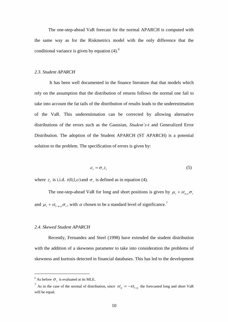
solution to the problem. The specification of errors is given by:

ttt z (5)

where tz is i.i.d. ),1,0( t and t is defined as in equation (4).

The one-step-ahead VaR for long and short positions is given by tt st ,

and tt st ,1 , with chosen to be a standard level of significance.7

2.4. Skewed Student APARCH

Recently, Fernandez and Steel (1998) have extended the student distribution

with the addition of a skewness parameter to take into consideration the problems of

skewness and kurtosis detected in financial databases. This has led to the development

6 As before t is evaluated at its MLE.

7 As in the case of the normal of distribution, since 1stst the forecasted long and short VaR

will be equal.

11

of the skewed student APARCH. However, their approach has the disadvantage that

this proposed skewness parameter is expressed in terms of the mode and the

dispersion. To avoid this deficiency Lambert and Laurent (2001) have re-expressed

the skewed student density in terms of the mean and the variance by a re-

parameterization of the density so that the innovation process has zero mean and unt

variance.8

We draw mainly on Giot and Laurent (2003) and we provide a discussion of

the statistical properties of the skewed Student APARCH model based on the

approach suggested by Lambert and Laurent (2001).

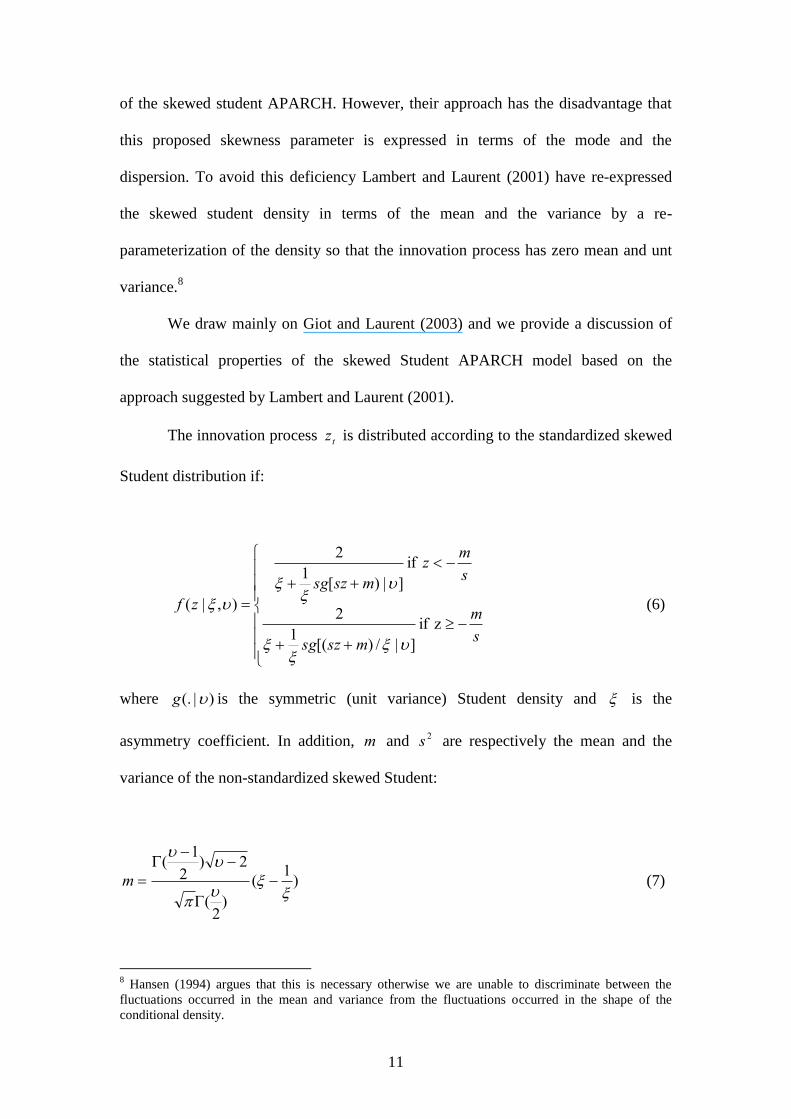
The innovation process tz is distributed according to the standardized skewed

Student distribution if:

s

m

mszsg

s

mz

mszsg

zf

z if

]|/)[(1

2

if

]|)[1

2

),|(

(6)

where )|(. g is the symmetric (unit variance) Student density and is the

asymmetry coefficient. In addition, m and 2s are respectively the mean and the

variance of the non-standardized skewed Student:

)1

(

)2

(

2)2

1(

m (7)

8 Hansen (1994) argues that this is necessary otherwise we are unable to discriminate between the

fluctuations occurred in the mean and variance from the fluctuations occurred in the shape of the

conditional density.

12

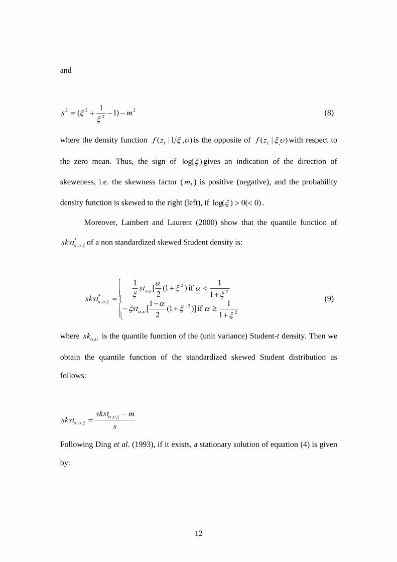
and

2

2

22 )11

( ms

(8)

where the density function ),1|( tzf is the opposite of )|( ,tzf with respect to

the zero mean. Thus, the sign of )log( gives an indication of the direction of

skeweness, i.e. the skewness factor ( 3m ) is positive (negative), and the probability

density function is skewed to the right (left), if )0(0)log( .

Moreover, Lambert and Laurent (2000) show that the quantile function of

*

,, skst of a non standardized skewed Student density is:

2

2

,

2

2

,*

,,

1

1 if )]1(

2

1[

1

1 if )1(

2[

1

st

st

skstua

(9)

where ,sk is the quantile function of the (unit variance) Student-t density. Then we

obtain the quantile function of the standardized skewed Student distribution as

follows:

s

mskstskst

,,

,,

Following Ding et al. (1993), if it exists, a stationary solution of equation (4) is given

by:

13

11 )|(|1)(

zzEE

n

t (10)

which is a function of the density of z . Such a solution exists if

1)|(| 11 zzEV n

Ding et al. (1993) derived the expression for )|(| zzE n for the Gaussian

case. We can also show that for the standardized skewed Student distribution is given

as follows:

)2

()2()1

(

)2)(2

()2

1(

})1()1({)|(|

2

1

1)1(

zzE (11)

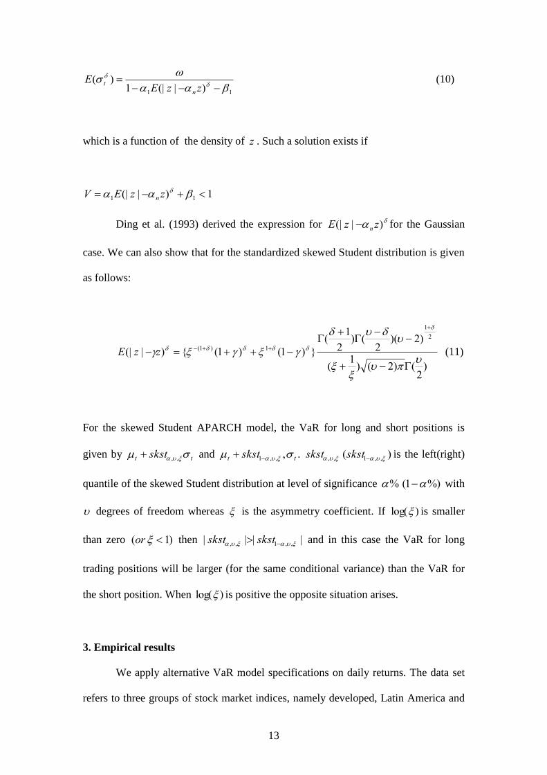
For the skewed Student APARCH model, the VaR for long and short positions is

given by tt skst ,, and tt skst ,,,1 . ,,skst )( ,,1 skst is the left(right)

quantile of the skewed Student distribution at level of significance % %)1( with

degrees of freedom whereas is the asymmetry coefficient. If )log( is smaller

than zero )1 ( or then |||| ,,1,, skstskst and in this case the VaR for long

trading positions will be larger (for the same conditional variance) than the VaR for

the short position. When )log( is positive the opposite situation arises.

3. Empirical results

We apply alternative VaR model specifications on daily returns. The data set

refers to three groups of stock market indices, namely developed, Latin America and

14

Asia/Pacific. Specifically, the following stock market indices data were used:

Australia (ALL ORDINATES, AOI); France (CAC40); Germany (DAX30); Greece

(FTSE20); Japan (NIKKEI225); Spain (MADRID General, SMSI); UK (FTSE100);

U.S.A (S&P 500); Argentina (MERVAL, MERV); Brazil (BOVESPA, BVSP);

Mexico (IPC); China (SHANGHAI Composite Index, SSG); Hong Kong (HANG

SENG Index, HSI); India (BOMBAY, BSE30); Indonesia (JAKARTA Composite,

JSX); Malaysia (Kuala Lumpur Composite Index, KLSE); Philippines (PSI);

Singapore (STRAIT TIMES Industrial Index, STII); South Korea (SEOUL

Composite, KOSPI); Sri Lanca (COLOMBO Index Average, CSE) and Taiwan

(Taiwan Weighted Stock Index, WEIGHTED). The starting year of the series under

consideration varies based on availability. The time span of the data sets is presented

in Table 1. All data sets end on December 31, 2009. The complete data set was

obtained from Datastream. Given the recent financial crisis of 2007-2009 it of crucial

importance to investigate the performance of the VaR measures of market risk for the

case of stocks traded in developed as well as in emerging markets. In order to

implement our analysis we construct historical portfolios for each case and we choose

a specification of the functional form of the distribution of returns. We successively

consider the Riskmetrics, normal APARCH, Student APARCH and skewed Student

APARCH. The estimation process is conducted for the full sample whereas we use

the last 5 years (each year is taken to have 252 trading days) to conduct the out-of-

sample forecasting evaluation.

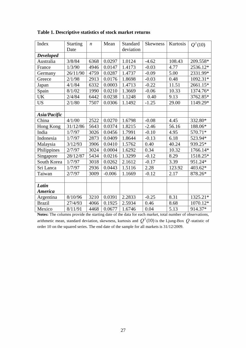
The daily returns are computed as 100 times the difference of the log of the

prices, i.e. )]ln()[ln(100 1 ttt ppy . Table 1 reports descriptive statistics for the

returns series. As it is expected higher returns are recorded for the emerging markets

compared to those of the developed markets. Moreover, according to the estimated

15

standard deviations it is clear that the developed markets are the less risky with the

exception Greece which although is considered a mature market it exhibited return

volatility compared to that of the emerging markets. We also observed that all 21

stock return series display similar statistical properties with respect to skewness and

kurtosis. Thus, the return series are skewed (either negatively or positively) whereas

the large returns (either positive or negative) lead to a large degree of kurtosis.

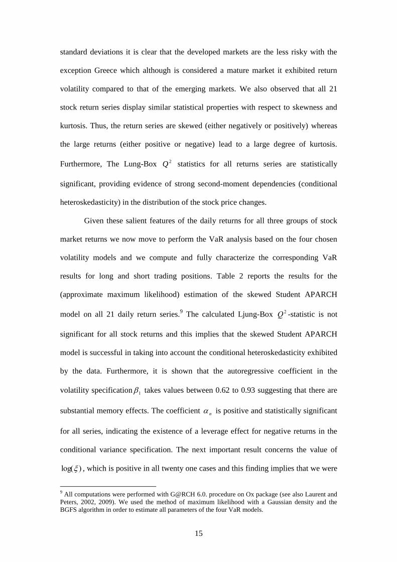
Furthermore, The Lung-Box 2Q statistics for all returns series are statistically

significant, providing evidence of strong second-moment dependencies (conditional

heteroskedasticity) in the distribution of the stock price changes.

Given these salient features of the daily returns for all three groups of stock

market returns we now move to perform the VaR analysis based on the four chosen

volatility models and we compute and fully characterize the corresponding VaR

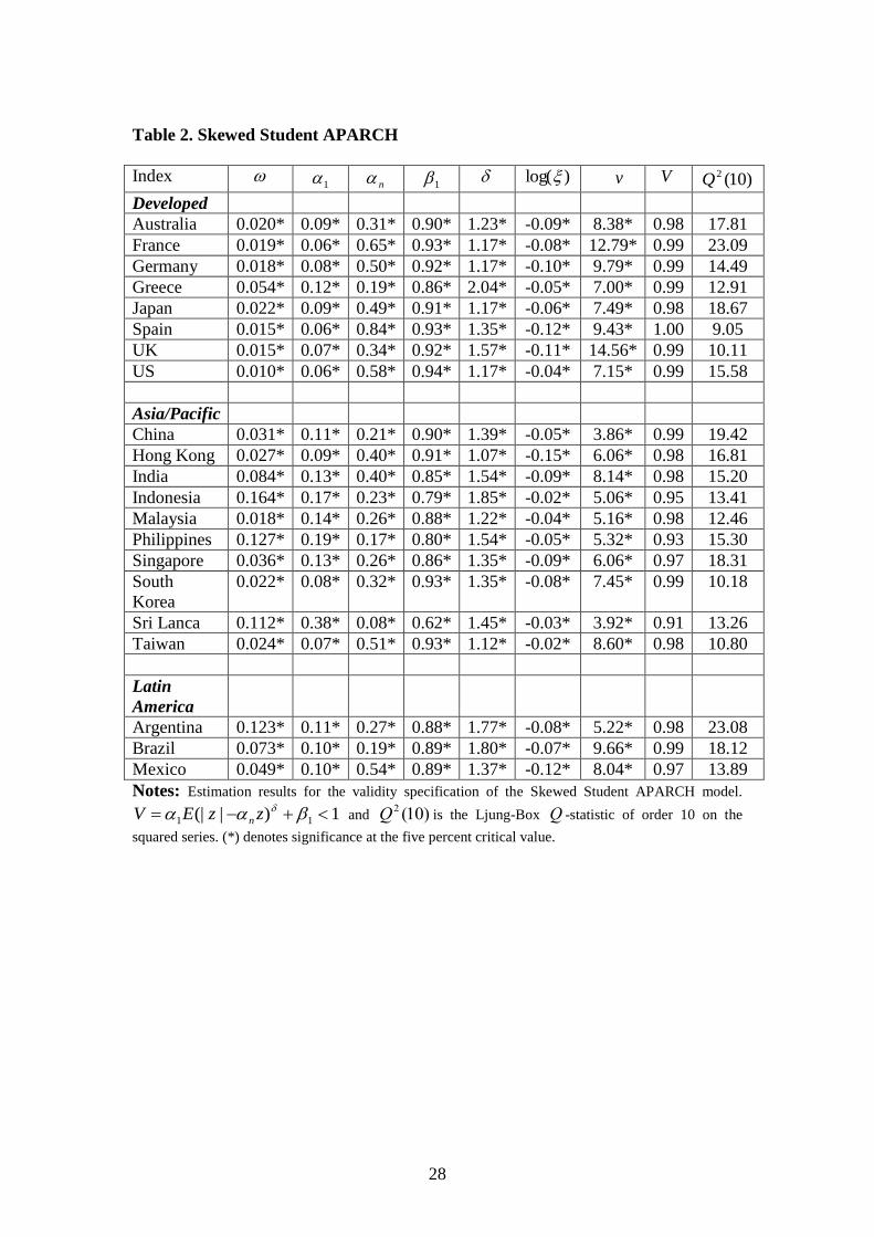
results for long and short trading positions. Table 2 reports the results for the

(approximate maximum likelihood) estimation of the skewed Student APARCH

model on all 21 daily return series.9 The calculated Ljung-Box 2Q -statistic is not

significant for all stock returns and this implies that the skewed Student APARCH

model is successful in taking into account the conditional heteroskedasticity exhibited

by the data. Furthermore, it is shown that the autoregressive coefficient in the

volatility specification 1 takes values between 0.62 to 0.93 suggesting that there are

substantial memory effects. The coefficient n is positive and statistically significant

for all series, indicating the existence of a leverage effect for negative returns in the

conditional variance specification. The next important result concerns the value of

)log( , which is positive in all twenty one cases and this finding implies that we were

9 All computations were performed with G@RCH 6.0. procedure on Ox package (see also Laurent and

Peters, 2002, 2009). We used the method of maximum likelihood with a Gaussian density and the

BGFS algorithm in order to estimate all parameters of the four VaR models.

16

correct in incorporating the asymmetry element in the Student distribution in order to

model the distribution of returns in an appropriate way. The final significant result

reported in Table 1 refers to the value of which takes values from 1.12 and 2.04

statistically significant from 2. In summary the above results indicate that the skewed

Student APARCH model takes into consideration the feature of a negative leverage

effect (conditional asymmetry) for the conditional variance and it is also consistent

with the fact that an asymmetric distribution for the error term (unconditional

asymmetry) exists.

We next moveδ to examine whether the skewed Student APARCH model

provides better VaR estimates and forecasting performance than the other three

models, Riskemetrics, normal APARCH and Student APARCH. To this end we move

on to provide in-sample VaR computations and this is accomplished by computing the

one-step-ahead VaR for all models. This procedure is equivalent to backtesting the

model on the estimation sample. We test all models with a VaR level of significance,

)( , that takes values from 0.25% to 5% and we then evaluate their performance by

calculating the failure rate for the returns series ty . The failure rate is defined as the

number of times returns exceed the forecasted VaR. Following Giot and Laurent

(2003) we define a failure rate lf for the long trading positions, which is equal to the

percentage of negative returns smaller than one-step-ahead VaR for long positions. In

a similar manner, we define sf as the failure rate for short positions as the percentage

of positive returns larger than the one-step-ahead VaR for short position.10

To evaluate the in-sample forecasting ability of the alternative VaR measures

we employ the unconditional backtesting criterion developed by Kupiec (1995). This

10

When the VaR model is correctly specified then the failure rate should be equal to the pre-specified

VaR level.

17

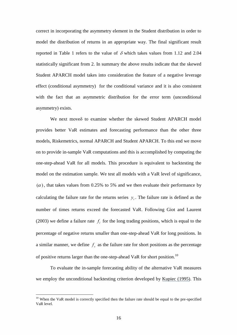
criterion tests the hypothesis that the proportion of violations (failures) is equal to the

expected one.11

Under the null hypothesis Kupiec (1995) developed a likelihood ratio

statistic given as follows:

2

1

^

~})1ln[(2]]1ln[2 NNTNT

uc fffNfLR (12)

where TNf is the failure rate, ^

f is the empirical (estimated) failure rate, N is

the number of days over a period T that a violation has occurred. Giot and Laurent

(2003) suggest that the computation of the empirical failure rate defines a sequence of

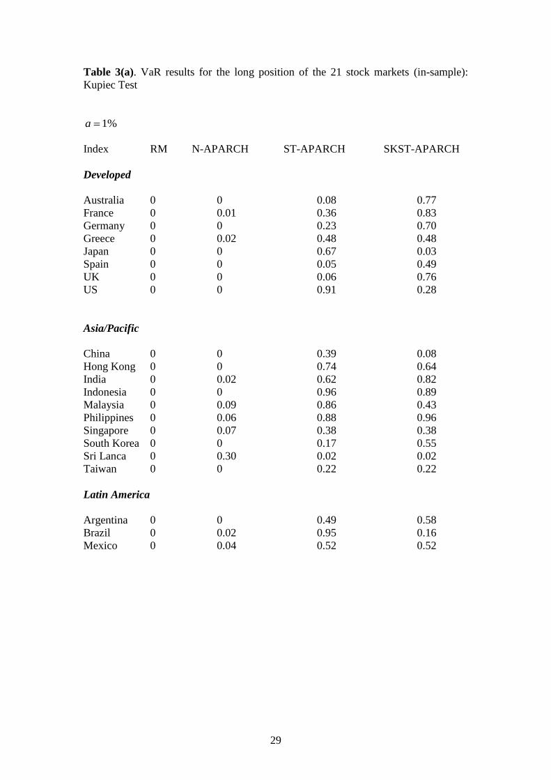
yes/no, under this testable hypothesis. Table 3(a)-(d) reports the corresponding p -

values for the four VaR models and for given significance levels.12

Based on the

results of the in-sample VaR computations we can arrive at the following conclusions:

For the long position with %1 VaR models based on the normal distribution (i.e.

Riskmetrics and normal APARCH model) perform a particularly poor job in

modelling large positive and negative returns, indicating that they generate biased

VaR estimates. The symmetric Student APARCH model provides substantially better

results compared to those of the normal model. Finally, the skewed Student APARCH

model provides the best performance of all VaR models for both negative and positive

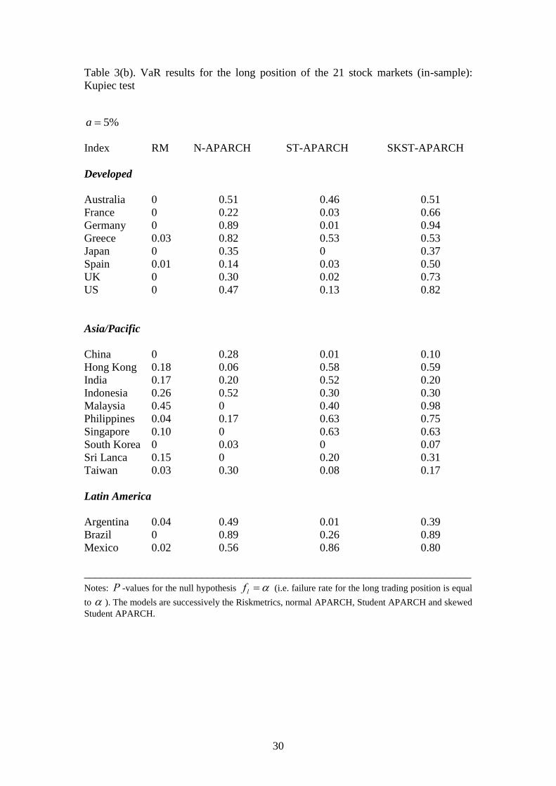
returns. In the relatively less extreme case of a 5% VaR we observed that

Riskemetrics still have a difficult job in modelling large positive and negative returns

for the developed and Latin America stock markets but is doing a fairly good job in

most of the Asia/Pacific markets. The normal APARCH has partially improved its

11

A violation is defined as the case where the predicted VaR is unable to cover the realized loss (or to

foresee the realized profit) 12

To save space we report only the results for 1% and 5%. However the results for the other values of

are consistent with those for 1% and 5%. These results are available upon request.

18

performance since it provides accurate VaR estimates for all developed and Latin

America markets although it fails to do so for most of the markets of the Asia/Pacific

region. The symmetric Student APARCH performs well for most of the stock markets

except for the cases of Japan and South Korea whereas the skewed Student APARCH

performs exceptionally well.

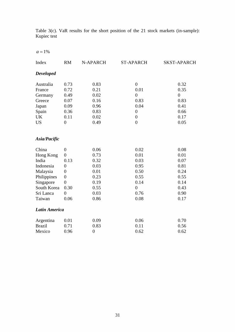
In the short position with %1 we observed that the Riskmetrics model

provides accurate VaR estimates for all the developed markets except the US and for

the Latin America markets but not for most of the Asia/Pacific markets. An

interesting finding is that the normal APARCH performs better than the symmetric

Student APARCH model but is again the skewed Student APARCH that performs

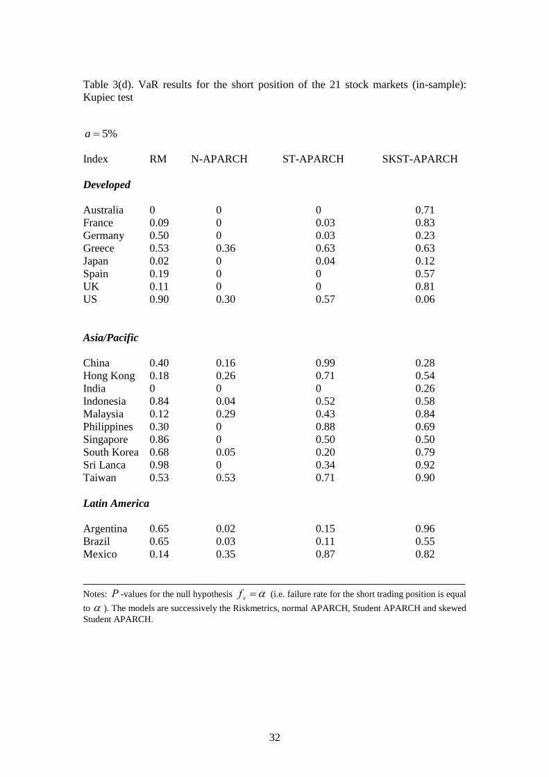
better in terms of the insignificance of the Kupiec test. Looking at the 5%VaR results

we observe that the Riskemetrics model performs well since except for Australia and

India all Kupiec statistics are insignificant, and in fact much better than either the

normal APARCH or the symmetric Student APARCH. Again, the best performance is

given by the skewed Student APARCH. This apparent asymmetry in the performance

of the Riskemetrics model between the long and short positions may be the result of

skewed distribution of returns it may also be due to the volatility asymmetry effect in

response to good and bad news.

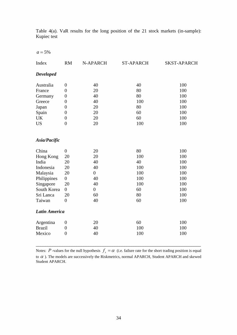
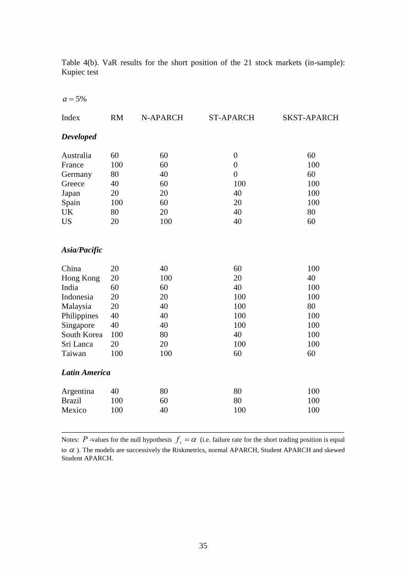
The picture that emerges from Table 4(a)-(b) further reinforces the superiority

of the skewed Student APARCH model over the alternative specifications. Indeed,

this specification performs correctly in 100% of all cases for the negative returns

(long position) and with only few exceptions for the positive returns (short position).

Moreover, we note that the skewed Student APARCH performs better that the student

APARCH since it corrects a number of deficiencies that the latter model has inherited

as a result of its conservatism.

19

Engle and Manganelli (2004) argued that the Kupiec test is an unconditional

test of VaR accuracy which given the substantial time-variation within volatility may

lead to incorrect conclusions and therefore conditional accuracy of the VaR

estimates must be considered. Therefore, in a correctly specified VaR model we

should not only examine whether the exceptions occur at the specified rate (i.e. 1% or

5%) but we also examine whether these exceptions are not serially correlated. To

this end Engle and Manganelli (2004) proposed the following Dynamic Quantile test

statistic (DQ) which takes this issue into consideration. Engle and Manganelli

(2004) define the following sequence:

( )k k kHit I r VaR a

Thus, this sequence takes the value (1 — α) in the case that the stock returns, kr are

less than the VaR quantile and the value (α) otherwise, with the expected value of

kHit equal to zero. Within this setting the Kupie test is a sub-case since although it

tests that this sequence will be the correct fraction of exceptions it does not test the null

hypothesis that this sequence is uncorrelated with past information and have a mean

value of zero, which implies that the hits will not be autocorrelated. To test the null

hypothesis of no serial correlation in the hit sequence kHit Engle and Manganelli

(2004) proposed to run a regression on file lags (days) and the current VaR estimate.

The DQ test statistic is then computed as: ^ ^

' ' / (1 )DQ X X where X is the

vector of explanatory variables and ^

the OLS estimates. The DQ test is distributed as

a 2x with degrees of freedom equal to the number of parameters.

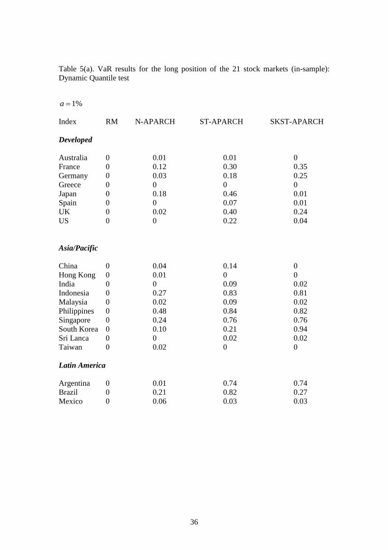
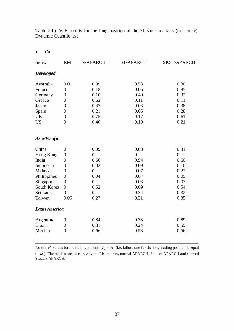
Tables 5(a)-(d) provide the evidence from the application of the DQ statistic

for the in-sample performance of the four competing models. For the case of the long

position and at both 1% and 5% VaR the Riskmetrics model performs the worst

20

across all markets, and the normal APARCH and the Symmetric Student APARCH

provide almost equivalent VaR accuracy as with the Kupiec test. The superiority of

the Skewed Student APARCH is confirmed again with the use of the most restricted

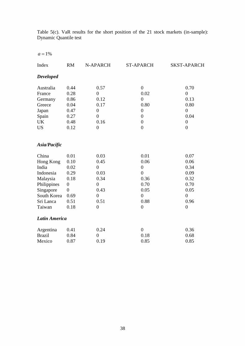
DQ test. Examining the case for the short position we notably observed that the

Riskmetrics model performs much better than the normal APARCH and the

Symmetric Student APARCH. Again, this asymmetric result may be due to skewed

distribution of returns and/or volatility asymmetry in response to good and bad news.

Finally, the Skewed Student APARCH performs better than its competing models.

We further assess the performance of the four models by computing the out-

of-sample VaR forecasts. This is considered as the „true‟ test for any VaR model. Out-

of-sample evaluation of a specific model requires the estimation of the model for the

known data points and then based on the estimated equation and we then provide

forecasts for a specific time horizon. This testing procedure is implemented to provide

one-day-ahead VaR forecasts.13

Following Giot and Laurent (2003) we apply an

iterative procedure in which the estimated model for the whole sample is estimated

and we then compare the predicted one-day-ahead VaR for both the long and short

positions with the actual return. This procedure is repeated for all known observations

and every time the estimation sample includes one more day and we forecast the

corresponding VaR. These forecasts are saved and they are used for the evaluation of

the out-of-sample predictive performance of the models.14

The iteration procedure

ends when, as it is the common practice, we have included the 1t days in the

estimation of the model. The predictive performance of the skewed Student APARCH

13

Christoffersen and Diebold (2000) document that the ARCH-class of models exhibit good volatility

forecastability for short horizon their performance is poor when it comes to long horizon prediction.

Although the latter may be more important for portfolio managers we only provide short run analysis

of predictive performance. 14

To conduct our out-of-sample forecasting analysis we employ the last five years (1260 obs.) of our

sample. We also use a „stability window‟ of 50 days to update the model parameters.

21

model is the evaluated using the Kupiec (1995) likelihood ratio test as in the in-

sample case. However, this time the failure rate was calculated for both the long and

short positions by comparing the corresponding forecasted 1tVaR with the observed

return 1ty .

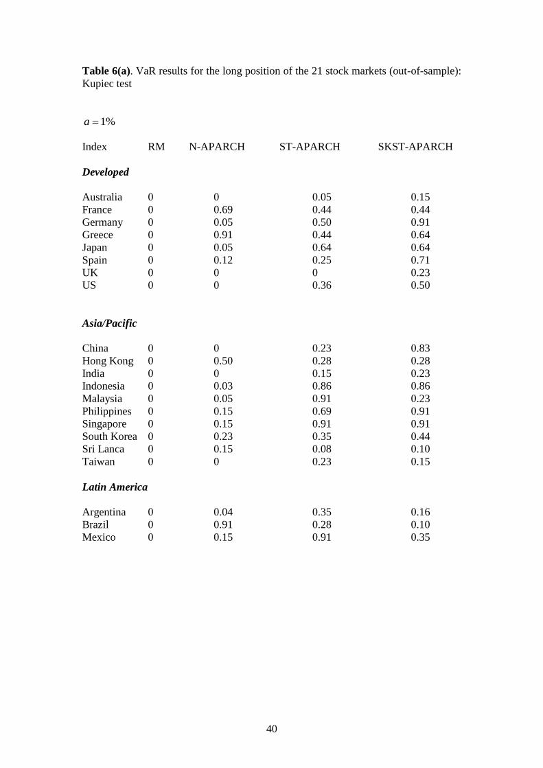
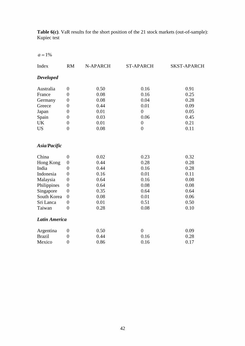
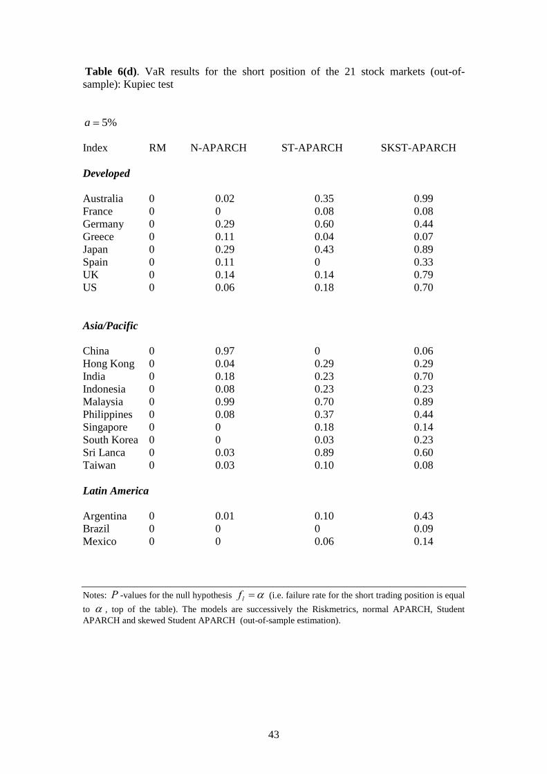
The results obtained from the Kupiec test for all return series are given in

Table 6(a)-(d). Like Table 3(a)-(d) we report the calculated p -values for alternative

level of significance for both long and short trading positions. These findings revealed

that Riskemetrics has a very poor out-of-sample forecasting performance in both long

and short trading positions making this model an inappropriate specification for

financial institutions to rely upon especially during very turbulent periods like the

2007-2009 financial crisis. For the long position the normal APARCH and the

Symmetric Student APARCH perform fairly well in out-of-sample prediction VaR

accuracy and their results are similar to the in-sample ones although the former misses

out Australia, UK and US, China, India and Taiwan and the latter the UK. Turning

our attention to the skewed Student APARCH model we concluded that it performs

well for out-of-sample VaR prediction for both long and short trading positions and

for both 1% and 5% VaR. Furthermore, we note that the combined (i.e. long and short

VaR) success rate is equal to 100% in all three groups of stock returns and this finding

further reinforces the suitability of the skewed Student APARCH model in measuring

market risk in developed and emerging.

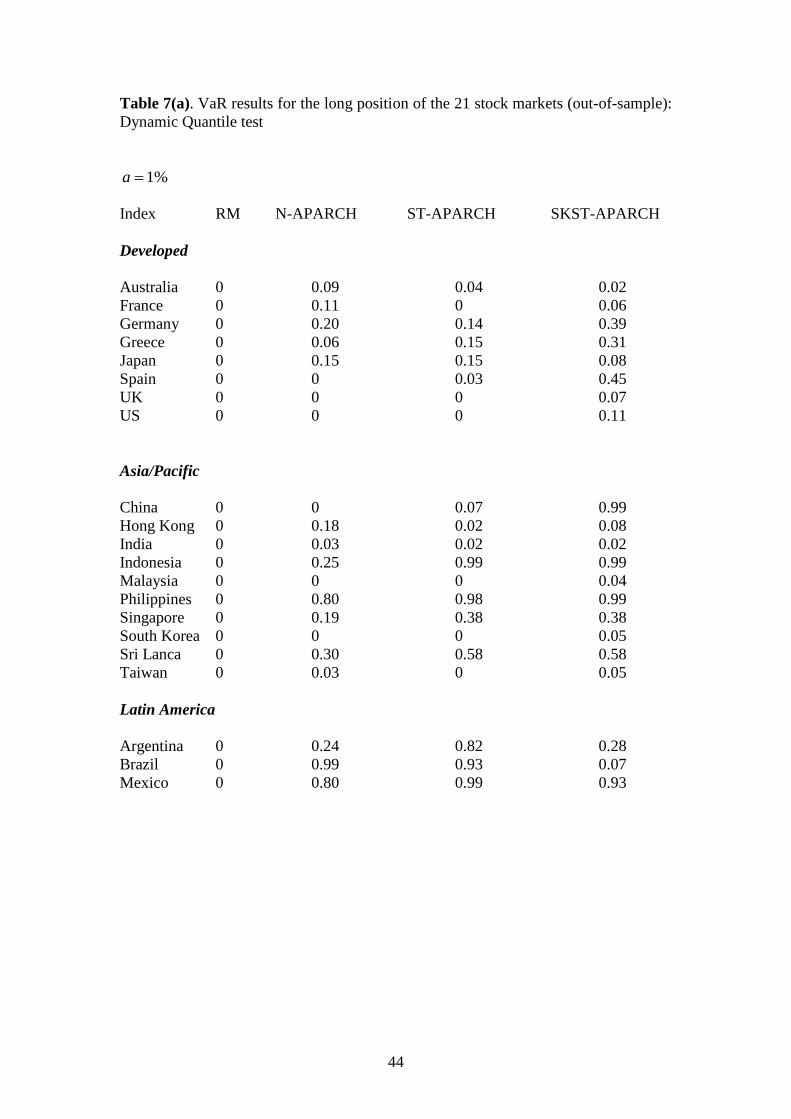
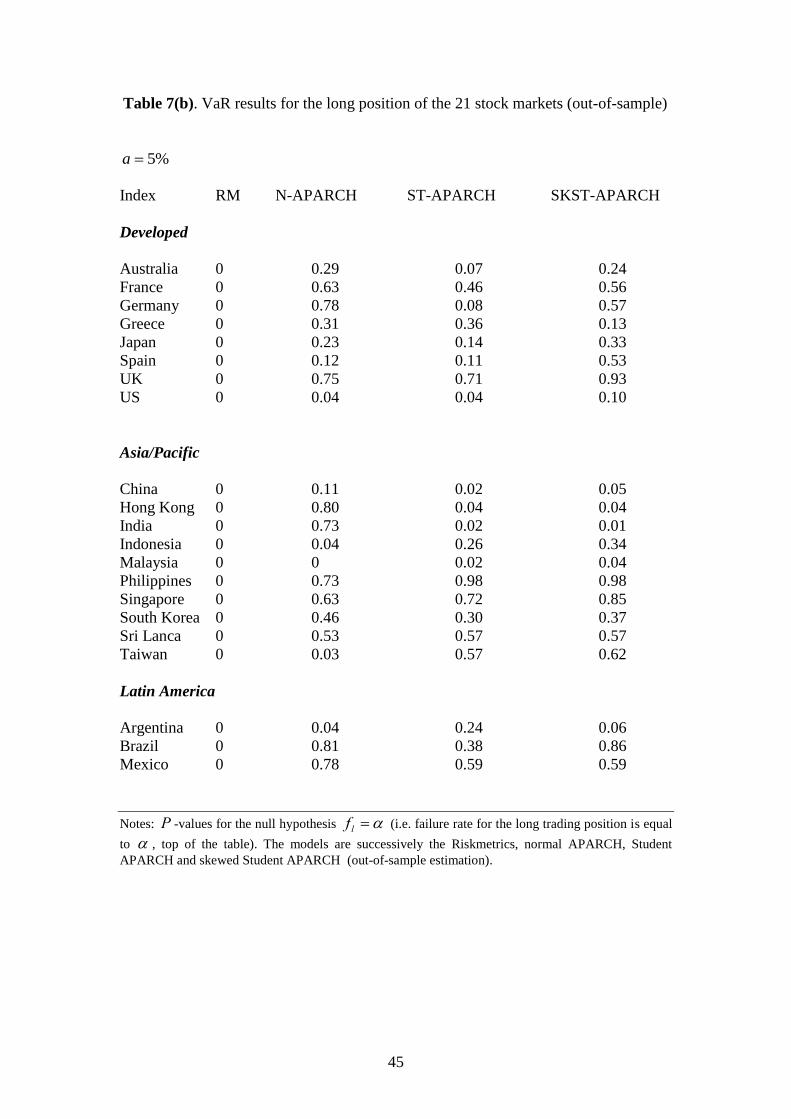
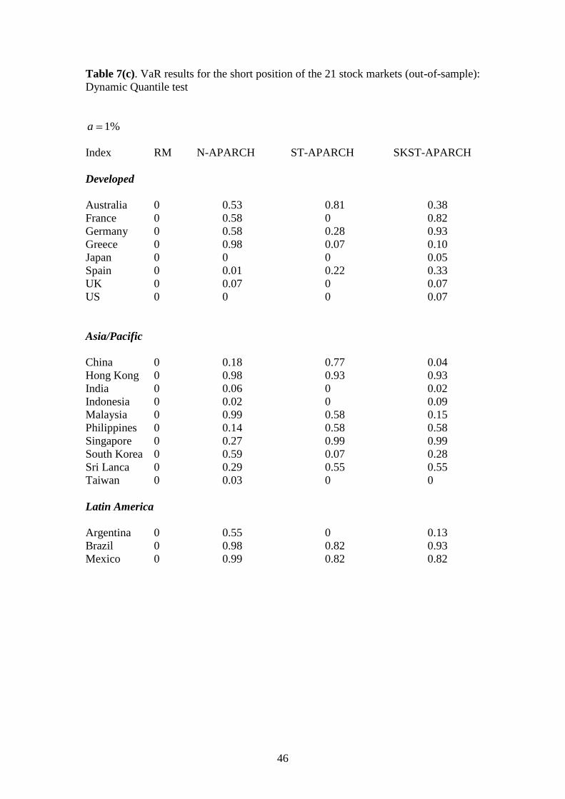
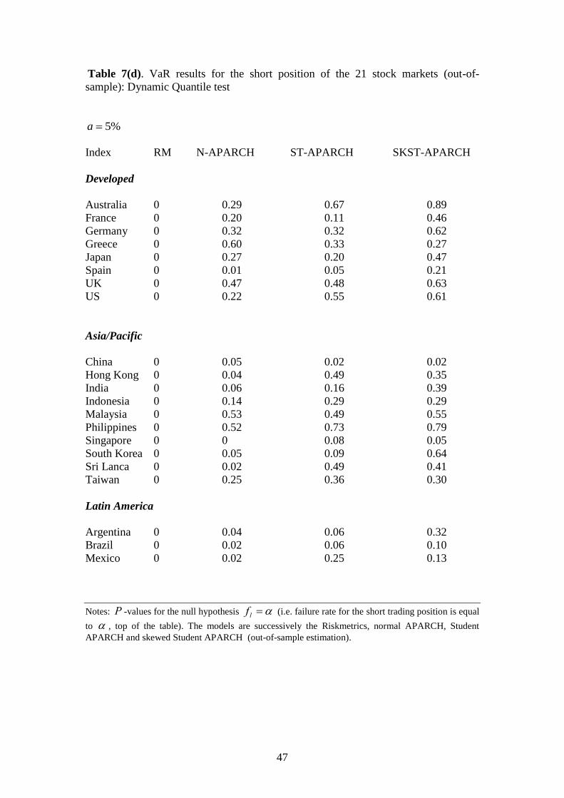
The results from the application of the DQ test for the out-of-sample

performance of the four VaR models are given in Tables 7(a)-(d). The overall

evidence is very similar to the one obtained from the Kupiec test. Riskemetrics is

again a poor model in predicting VaR accuracy for all twenty one markets. Normal

APARCH and Symmetric Student APARCH improve considerably on the

22

performance of the Riskemetrics model but their performance is still not satisfactory

in all cases. The skewed Student APARCH model improves on all other specifications

for both negative and positive returns and for either 1% or 5% critical level. The

model performs correctly in 100% of all cases for the long position and for the short

position.15

4. Summary and conclusions

During the last decade we have observed a substantial change in the way

financial institutions evaluate risk. Faced with increased volatility of stock returns as

well as with the heavy losses that banks and securities houses have experienced

portfolio managers and supervising committees of financial markets have sought for a

continuous improvement to potential measures of market risk. Value at Risk is one of

the major tools for measuring market risk on a daily basis and is recommended by the

Basel Committee on Banking Supervision and this is documented in the Basel Accord

Amendment of 1996.

These models of risk management have become the standard tool for

measuring internal risk management as well as for external regulatory purposes.

However, most of the recent applications of evaluating VaRs for a wide range of

markets have mostly applied for the case of negative returns, i.e. for the negative tail

of the distribution of returns. The present paper deals with modeling VaR for

portfolios that includes both long and short positions. Therefore, we consider the

modeling and calculation of VaR for portfolio managers who have taken either a long

position (bought an asset) or a short position (sold an asset).

15

We have further tested the performance of the four models with the calculation of two additional

measures relevant to the VaR analysis: The expected shortfall (Scaillet, 2000) and the average multiple

of tail event to risk measure (Hendricks (1996). Both measures provide additional support in favour of

the skewed Student APARCH model. To save space the results are available upon request.

23

The financial crisis of 2007-2009 has raised questions regarding the usefulness

of the regulatory framework underlined by the Basle I and II agreements and it also

questioned the appropriateness of the VaR as the measure to capture extreme cases

like the ones the banking sector and global financial markets experienced over this

turbulent period since several financial institutions went bankrupt under these extreme

conditions.

This paper extends previous works on the forecasting performance of

alternative VaR models. Specifically, we focused on the comparison of four

alternative models for the estimation of one-step-ahead VaR for long and short trading

positions. We have applied a battery of univariate tests on four parametric VaR

models namely, RiskMetrics, normal APARCH, Student APARCH and skewed

Student APARCH. We employed data that covered the recent financial crisis of 2007-

2009 for twenty of stock markets which included both developed and emerging stock

markets. Our purpose was twofold. First we seek to examine whether alternative VaR

models provide different evidence for the case of developed as opposed to the

emerging markets and second. We examined the performance of these models when

periods of turbulence are included in the sample. Our overall results lead to the

overwhelming conclusion that the skewed Student APARCH model outperforms all

other specification modelling VaR for either long or short positions. These findings

confirmed earlier evidence which show that models which include an asymmetric

parameter perform substantially better than those with normal errors and this

asymmetric feature is important in forecasting accuracy of the VaR models.

24

References

Alexander, C., 2003, Market Models: A Guide to Financial Data Analysis, New York:

John Wiley

Alexander, S., 2005, The present and future of financial risk management, Journal of

Financial Econometrics, 3, 3-25.

Bank for International Settlements, 1988, International convergence of capital

measurement and capital standards, BCBS Publication Series, No. 4.

Bank for International Settlements, 1999a, Capital requirements and bank behavior:

The impact of the Basle accord, BCBS Working Paper Series, No. 1.

Bank for International Settlements, 1999b, A new capital adequacy framework, BCBS

Publications Series, No. 50.

Bank for International Settlements, 1999c, Supervisory lesson to be drawn from the

Asian crisis, BCBS Working paper series, No. 2.

Bank for International Settlements, 2001, The New Basel Capital Accord, BIS, Basel.

Basel Committee on Banking Supervision, 1996, Amendment to the Capital Accord

to incorporate market risks.

Bera, A.K. and M.L. Higgins, 1993, ARCH models: Properties, estimation and

testing, Journal of Economic Surveys,

Black, F., 1976, Studies of stock market volatility changes, Proceedings of the

American Statistical Association, Business and Statistics Section, 177-181.

Bollerslev, T., 1986, Generalized autoregressive conditional heteroskedasticity,

Journal of Econometrics, 31, 307-327.

Bollerslev, T., 1990, modelling the coherence in short-run nominal exchange rates: A

multivariate generalized arch model, Review of Economics and Statistics, 72, 498-

505.

Bollerslev, T, R.F. Engle and J.M. Wooldridge, 1988, A capital asset pricing model

with time varying covariances, Journal of Political Economy, 96, 116-131.

Brooks, C. and G. Persand, 2000, Value-at-risk and market crashes, Discussion Paper

in Finance 2000-01, University of Reading ISMA Centre.

Brunnermeier, M.K., 2009, Deciphering the liquidity and credit crunch 2007-2008,

Journal of Economic Perspectives, 23, 77-100.

Campbell, J.Y., A.W. Lo and A.C. MacKinlay, 1997, The Econometrics of Financial

Markets, Princeton University Press, NJ.

25

Cristoffersen, P.F. and F.X. Diebold, 2000, How relevant is volatility forecasting for

financial risk management? Review of Economics and Statistics, 82, 1-11.

Day, T.E. and C. M. Lewis, 1992, Stock market volatility and the information content

of stock price options, 52, 267-287.

De Grauwe, P., 2009, The Banking crisis: causes, consequences and remedies,

Universite Catholique de Louvain, mimeo.

Ding, Z., C.W.J. Granger and R.F. Engle, 1993, A long memory property of stock

market returns and a new model, Journal of Empirical Finance, 1, 83-106.

El Babsiri, M. and J-M. Zakoian, 2001, Contemporaneous asymmetry in GARCH

processes, Journal of Econometrics, 101, 257-294.

Engle, R.F., 1982, Autoregressive conditional heteroskedasticity with estimates of the

variance of the united kingdom inflation, Econometrica, 50, 987-1007.

Engle, R.F, 2002, New frontiers for ARCH models, Journal of Applied Econometrics,

17, 425-446.

Engle, R.F., 2002, Dynamic conditional correlation: a simple class of multivariate

GARCH models, Journal of Business and Economics Statistics, 20, 339-350.

Engle, R.F. and S. Manganelli, 2004, CAViaR: Conditional autoregressive Value at

Risk by regression quantile, Journal of Business and Economic Statistics, 22, 367-

381.

French, K.R., G.W. Schwert and R.F. Stambaugh, 1987, Expected stock returns and

volatility, Journal of Financial Economics, 19, 3-29.

Giot, P. and S. Laurent, 2003, Value-at-Risk for long and short trading positions,

Journal of Applied Econometrics, 18, 641-664.

Hansen, B.E., 1994, Autoregressive conditional density estimation, International

Economic Review, 35, 705-730.

Harvey, C.R. and A. Siddique, 1999, Autoregressive conditional skewness, Journal of

Financial and Quantitative Analysis, 34, 465-487.

He, C. and T. Terasvista, 1999a, Higher-order dependence in the general power

ARCH process and a special case, Stockholm School of Economics, Working Paper

Series in Economics and Finance, No. 315.

Hendricks, D., 1996, Evaluation of value-at-risk models using historical data, Federal

Reserve Bank of New York Economic Policy Review, April.

Jorion, P., 2000, Value at Risk, 2nd

ed., New York: McGraw Hill.

26

Kroner, F.K. and V.K. Ng, 1998, Modelling asymmetric comovements of asset

returns, The Review of Financial Studies, 11, 817-844.

Kupiec, P., 1995, Techniques for verifying the accuracy of risk measurement models,

Journal of Derivatives, 2, 174-184.

Lambert, P. and S. Laurent, 2000, Modelling skewness dynamics in series of financial

data, Discussion Paper, Institut de Statistique, Louvain-la-Neuve.

Lambert, P. and S. Laurent, 2001, Modelling financial time series using GARCH-type

models and a skewed density, Universite de Liege, mimeo.

Lambert, P. and J-P Peters, 2002, G@RCH 2.2: An Ox package for estimating and

forecasting various ARCH models, Journal of Economic Surveys, 16, 447-485.

Laurent, S. and J-P Peters, 2009, Estimating and forecasting ARCH Models using

G@RCH 6.0 Timberlake Consultants.

Manganelli, S. and R.F. Engle, 2001, Value at risk models in finance, Working Paper

075, European Central Bank.

McMillan, D.G. and A. E.H. Speight, 2007, Value-at-Risk in emerging equity

markets: Comparative evidence for symmetric, asymmetric and long-memory

GARCH models, International Review of Finance, 7, 1-19.

McMillan, D. G. and D. Kambouroudis, 2009, Are RiskMetrics forecasts good

enough? Evidence from 31 stock markets, International Review of Financial Analysis,

18, 117-124.

Pagan, A. and G. Schwert, 1990, Alternative models for conditional stock volatility,

Journal of Econometrics, 45, 267-290.

RiskMetrics, 1996, Technical Document, Morgan Guarantee Trust Company of New

York.

Scaillet, O., 2000, Nonparametric estimation and sensitivity analysis of expected

shortfall, Universite Catholique de Louvain, IRES, mimeo.

So, M.K.P. and P.L.H. Yu, 2006, Empirical analysis of GARCH models in value at

risk estimation, Journal of International Financial Markets, Institutions and Money,

16, 180-197.

Tang, T-L and S-J Shieh, 2006, Long memory in stock index futures markets: A

value-at-risk approach, Physica A, 366, 437-448.

Taylor, S. J., 1986, Modelling Financial Time Series, New York: Wiley and Sons Ltd.

Welfens, P.J.J. 2009, The international banking crisis: lessons and EU reforms,

European Economy, 137-173.

27

Table 1. Descriptive statistics of stock market returns

Index Starting

Date

n Mean Standard

deviation

Skewness Kurtosis )10(2Q

Developed

Australia 3/8/84 6368 0.0297 1.0124 -4.62 108.43 209.558*

France 1/3/90 4946 0.0147 1.4173 -0.03 4.77 2536.12*

Germany 26/11/90 4759 0.0287 1.4737 -0.09 5.00 2331.99*

Greece 2/1/98 2913 0.0176 1.8698 -0.03 0.48 1092.31*

Japan 4/1/84 6332 0.0003 1.4713 -0.22 11.51 2661.15*

Spain 8/1/02 1990 0.0210 1.3669 -0.06 10.33 1374.76*

UK 2/4/84 6442 0.0238 1.1248 0.40 9.13 3762.85*

US 2/1/80 7507 0.0306 1.1492 -1.25 29.00 1149.29*

Asia/Pacific

China 4/1/00 2522 0.0270 1.6798 -0.08 4.45 332.80*

Hong Kong 31/12/86 5643 0.0374 1.8215 -2.46 56.16 188.06*

India 1/7/97 3026 0.0456 1.7991 -0.10 4.95 570.71*

Indonesia 1/7/97 2873 0.0409 1.8644 -0.13 6.18 523.94*

Malaysia 3/12/93 3906 0.0410 1.5762 0.40 40.24 939.25*

Philippines 2/7/97 3024 0.0004 1.6292 0.34 10.32 1766.14*

Singapore 28/12/87 5434 0.0216 1.3299 -0.12 8.29 1518.25*

South Korea 1/7/97 3018 0.0262 2.1612 -0.17 3.39 951.24*

Sri Lanca 1/7/97 2936 0.0443 1.5116 2.28 123.92 403.62*

Taiwan 2/7/97 3009 -0.006 1.1669 -0.12 2.17 878.26*

Latin

America

Argentina 8/10/96 3210 0.0391 2.2833 -0.25 8.31 1325.21*

Brazil 27/4/93 4066 0.1925 2.5934 0.46 8.68 1070.12*

Mexico 8/11/91 4468 0.0677 1.6746 0.04 5.13 914.37* Notes: The columns provide the starting date of the data for each market, total number of observations,

arithmetic mean, standard deviation, skewness, kurtosis and )10(2Q is the Ljung-Box Q -statistic of

order 10 on the squared series. The end date of the sample for all markets is 31/12/2009.

28

Table 2. Skewed Student APARCH

Index 1 n 1 )log( v V )10(2Q

Developed

Australia 0.020* 0.09* 0.31* 0.90* 1.23* -0.09* 8.38* 0.98 17.81

France 0.019* 0.06* 0.65* 0.93* 1.17* -0.08* 12.79* 0.99 23.09

Germany 0.018* 0.08* 0.50* 0.92* 1.17* -0.10* 9.79* 0.99 14.49

Greece 0.054* 0.12* 0.19* 0.86* 2.04* -0.05* 7.00* 0.99 12.91

Japan 0.022* 0.09* 0.49* 0.91* 1.17* -0.06* 7.49* 0.98 18.67

Spain 0.015* 0.06* 0.84* 0.93* 1.35* -0.12* 9.43* 1.00 9.05

UK 0.015* 0.07* 0.34* 0.92* 1.57* -0.11* 14.56* 0.99 10.11

US 0.010* 0.06* 0.58* 0.94* 1.17* -0.04* 7.15* 0.99 15.58

Asia/Pacific

China 0.031* 0.11* 0.21* 0.90* 1.39* -0.05* 3.86* 0.99 19.42

Hong Kong 0.027* 0.09* 0.40* 0.91* 1.07* -0.15* 6.06* 0.98 16.81

India 0.084* 0.13* 0.40* 0.85* 1.54* -0.09* 8.14* 0.98 15.20

Indonesia 0.164* 0.17* 0.23* 0.79* 1.85* -0.02* 5.06* 0.95 13.41

Malaysia 0.018* 0.14* 0.26* 0.88* 1.22* -0.04* 5.16* 0.98 12.46

Philippines 0.127* 0.19* 0.17* 0.80* 1.54* -0.05* 5.32* 0.93 15.30

Singapore 0.036* 0.13* 0.26* 0.86* 1.35* -0.09* 6.06* 0.97 18.31

South

Korea

0.022* 0.08* 0.32* 0.93* 1.35* -0.08* 7.45* 0.99 10.18

Sri Lanca 0.112* 0.38* 0.08* 0.62* 1.45* -0.03* 3.92* 0.91 13.26

Taiwan 0.024* 0.07* 0.51* 0.93* 1.12* -0.02* 8.60* 0.98 10.80

Latin

America

Argentina 0.123* 0.11* 0.27* 0.88* 1.77* -0.08* 5.22* 0.98 23.08

Brazil 0.073* 0.10* 0.19* 0.89* 1.80* -0.07* 9.66* 0.99 18.12

Mexico 0.049* 0.10* 0.54* 0.89* 1.37* -0.12* 8.04* 0.97 13.89

Notes: Estimation results for the validity specification of the Skewed Student APARCH model.

1)|(| 11 zzEV n and )10(2Q is the Ljung-Box Q -statistic of order 10 on the

squared series. (*) denotes significance at the five percent critical value.

29

Table 3(a). VaR results for the long position of the 21 stock markets (in-sample):

Kupiec Test

%1a

Index RM N-APARCH ST-APARCH SKST-APARCH

Developed

Australia 0 0 0.08 0.77

France 0 0.01 0.36 0.83

Germany 0 0 0.23 0.70

Greece 0 0.02 0.48 0.48

Japan 0 0 0.67 0.03

Spain 0 0 0.05 0.49

UK 0 0 0.06 0.76

US 0 0 0.91 0.28

Asia/Pacific

China 0 0 0.39 0.08

Hong Kong 0 0 0.74 0.64

India 0 0.02 0.62 0.82

Indonesia 0 0 0.96 0.89

Malaysia 0 0.09 0.86 0.43

Philippines 0 0.06 0.88 0.96

Singapore 0 0.07 0.38 0.38

South Korea 0 0 0.17 0.55

Sri Lanca 0 0.30 0.02 0.02

Taiwan 0 0 0.22 0.22

Latin America

Argentina 0 0 0.49 0.58

Brazil 0 0.02 0.95 0.16

Mexico 0 0.04 0.52 0.52

30

Table 3(b). VaR results for the long position of the 21 stock markets (in-sample):

Kupiec test

%5a

Index RM N-APARCH ST-APARCH SKST-APARCH

Developed

Australia 0 0.51 0.46 0.51

France 0 0.22 0.03 0.66

Germany 0 0.89 0.01 0.94

Greece 0.03 0.82 0.53 0.53

Japan 0 0.35 0 0.37

Spain 0.01 0.14 0.03 0.50

UK 0 0.30 0.02 0.73

US 0 0.47 0.13 0.82

Asia/Pacific

China 0 0.28 0.01 0.10

Hong Kong 0.18 0.06 0.58 0.59

India 0.17 0.20 0.52 0.20

Indonesia 0.26 0.52 0.30 0.30

Malaysia 0.45 0 0.40 0.98

Philippines 0.04 0.17 0.63 0.75

Singapore 0.10 0 0.63 0.63

South Korea 0 0.03 0 0.07

Sri Lanca 0.15 0 0.20 0.31

Taiwan 0.03 0.30 0.08 0.17

Latin America

Argentina 0.04 0.49 0.01 0.39

Brazil 0 0.89 0.26 0.89

Mexico 0.02 0.56 0.86 0.80

_____________________________________________________________________

Notes: P -values for the null hypothesis lf (i.e. failure rate for the long trading position is equal

to ). The models are successively the Riskmetrics, normal APARCH, Student APARCH and skewed

Student APARCH.

31

Table 3(c). VaR results for the short position of the 21 stock markets (in-sample):

Kupiec test

%1a

Index RM N-APARCH ST-APARCH SKST-APARCH

Developed

Australia 0.73 0.83 0 0.32

France 0.72 0.21 0.01 0.35

Germany 0.49 0.02 0 0

Greece 0.07 0.16 0.83 0.83

Japan 0.09 0.96 0.04 0.41

Spain 0.36 0.83 0 0.66

UK 0.11 0.02 0 0.17

US 0 0.49 0 0.05

Asia/Pacific

China 0 0.06 0.02 0.08

Hong Kong 0 0.73 0.01 0.01

India 0.13 0.32 0.03 0.07

Indonesia 0 0.03 0.95 0.81

Malaysia 0 0.01 0.50 0.24

Philippines 0 0.23 0.55 0.55

Singapore 0 0.19 0.14 0.14

South Korea 0.30 0.55 0 0.43

Sri Lanca 0 0.03 0.76 0.90

Taiwan 0.06 0.86 0.08 0.17

Latin America

Argentina 0.01 0.09 0.06 0.70

Brazil 0.71 0.83 0.11 0.56

Mexico 0.96 0 0.62 0.62

32

Table 3(d). VaR results for the short position of the 21 stock markets (in-sample):

Kupiec test

%5a

Index RM N-APARCH ST-APARCH SKST-APARCH

Developed

Australia 0 0 0 0.71

France 0.09 0 0.03 0.83

Germany 0.50 0 0.03 0.23

Greece 0.53 0.36 0.63 0.63

Japan 0.02 0 0.04 0.12

Spain 0.19 0 0 0.57

UK 0.11 0 0 0.81

US 0.90 0.30 0.57 0.06

Asia/Pacific

China 0.40 0.16 0.99 0.28

Hong Kong 0.18 0.26 0.71 0.54

India 0 0 0 0.26

Indonesia 0.84 0.04 0.52 0.58

Malaysia 0.12 0.29 0.43 0.84

Philippines 0.30 0 0.88 0.69

Singapore 0.86 0 0.50 0.50

South Korea 0.68 0.05 0.20 0.79

Sri Lanca 0.98 0 0.34 0.92

Taiwan 0.53 0.53 0.71 0.90

Latin America

Argentina 0.65 0.02 0.15 0.96

Brazil 0.65 0.03 0.11 0.55

Mexico 0.14 0.35 0.87 0.82

_____________________________________________________________________

Notes: P -values for the null hypothesis sf (i.e. failure rate for the short trading position is equal

to ). The models are successively the Riskmetrics, normal APARCH, Student APARCH and skewed

Student APARCH.

33

34

Table 4(a). VaR results for the long position of the 21 stock markets (in-sample):

Kupiec test

%5a

Index RM N-APARCH ST-APARCH SKST-APARCH

Developed

Australia 0 40 40 100

France 0 20 80 100

Germany 0 40 80 100

Greece 0 40 100 100

Japan 0 20 80 100

Spain 0 20 60 100

UK 0 20 60 100

US 0 20 100 100

Asia/Pacific

China 0 20 80 100

Hong Kong 20 20 100 100

India 20 40 40 100

Indonesia 20 40 100 100

Malaysia 20 0 100 100

Philippines 0 40 100 100

Singapore 20 40 100 100

South Korea 0 0 60 100

Sri Lanca 20 60 80 100

Taiwan 0 40 60 100

Latin America

Argentina 0 20 60 100

Brazil 0 40 100 100

Mexico 0 40 100 100

_____________________________________________________________________

Notes: P -values for the null hypothesis sf (i.e. failure rate for the short trading position is equal

to ). The models are successively the Riskmetrics, normal APARCH, Student APARCH and skewed

Student APARCH.

35

Table 4(b). VaR results for the short position of the 21 stock markets (in-sample):

Kupiec test

%5a

Index RM N-APARCH ST-APARCH SKST-APARCH

Developed

Australia 60 60 0 60

France 100 60 0 100

Germany 80 40 0 60

Greece 40 60 100 100

Japan 20 20 40 100

Spain 100 60 20 100

UK 80 20 40 80

US 20 100 40 60

Asia/Pacific

China 20 40 60 100

Hong Kong 20 100 20 40

India 60 60 40 100

Indonesia 20 20 100 100

Malaysia 20 40 100 80

Philippines 40 40 100 100

Singapore 40 40 100 100

South Korea 100 80 40 100

Sri Lanca 20 20 100 100

Taiwan 100 100 60 60

Latin America

Argentina 40 80 80 100

Brazil 100 60 80 100

Mexico 100 40 100 100

_____________________________________________________________________

Notes: P -values for the null hypothesis sf (i.e. failure rate for the short trading position is equal

to ). The models are successively the Riskmetrics, normal APARCH, Student APARCH and skewed

Student APARCH.

36

Table 5(a). VaR results for the long position of the 21 stock markets (in-sample):

Dynamic Quantile test

%1a

Index RM N-APARCH ST-APARCH SKST-APARCH

Developed

Australia 0 0.01 0.01 0

France 0 0.12 0.30 0.35

Germany 0 0.03 0.18 0.25

Greece 0 0 0 0

Japan 0 0.18 0.46 0.01

Spain 0 0 0.07 0.01

UK 0 0.02 0.40 0.24

US 0 0 0.22 0.04

Asia/Pacific

China 0 0.04 0.14 0

Hong Kong 0 0.01 0 0

India 0 0 0.09 0.02

Indonesia 0 0.27 0.83 0.81

Malaysia 0 0.02 0.09 0.02

Philippines 0 0.48 0.84 0.82

Singapore 0 0.24 0.76 0.76

South Korea 0 0.10 0.21 0.94

Sri Lanca 0 0 0.02 0.02

Taiwan 0 0.02 0 0

Latin America

Argentina 0 0.01 0.74 0.74

Brazil 0 0.21 0.82 0.27

Mexico 0 0.06 0.03 0.03

37

Table 5(b). VaR results for the long position of the 21 stock markets (in-sample):

Dynamic Quantile test

%5a

Index RM N-APARCH ST-APARCH SKST-APARCH

Developed

Australia 0.01 0.99 0.53 0.30

France 0 0.18 0.06 0.85

Germany 0 0.10 0.40 0.32

Greece 0 0.63 0.11 0.11

Japan 0 0.47 0.03 0.38

Spain 0 0.21 0.06 0.28

UK 0 0.75 0.17 0.61

US 0 0.40 0.10 0.21

Asia/Pacific

China 0 0.09 0.08 0.31

Hong Kong 0 0 0 0

India 0 0.66 0.94 0.60

Indonesia 0 0.03 0.09 0.10

Malaysia 0 0 0.07 0.22

Philippines 0 0.04 0.07 0.05

Singapore 0 0 0.03 0.03

South Korea 0 0.52 0.09 0.54

Sri Lanca 0 0 0.34 0.32

Taiwan 0.06 0.27 0.21 0.35

Latin America

Argentina 0 0.84 0.33 0.89

Brazil 0 0.81 0.24 0.59

Mexico 0 0.66 0.53 0.56

_____________________________________________________________________

Notes: P -values for the null hypothesis sf (i.e. failure rate for the long trading position is equal

to ). The models are successively the Riskmetrics, normal APARCH, Student APARCH and skewed

Student APARCH.

38

Table 5(c). VaR results for the short position of the 21 stock markets (in-sample):

Dynamic Quantile test

%1a

Index RM N-APARCH ST-APARCH SKST-APARCH

Developed

Australia 0.44 0.57 0 0.70

France 0.28 0 0.02 0

Germany 0.86 0.12 0 0.13

Greece 0.04 0.17 0.80 0.80

Japan 0.47 0 0 0

Spain 0.27 0 0 0.04

UK 0.48 0.16 0 0

US 0.12 0 0 0

Asia/Pacific

China 0.01 0.03 0.01 0.07

Hong Kong 0.10 0.45 0.06 0.06

India 0.02 0 0 0.34

Indonesia 0.29 0.03 0 0.09

Malaysia 0.18 0.34 0.36 0.32

Philippines 0 0 0.70 0.70

Singapore 0 0.43 0.05 0.05

South Korea 0.69 0 0 0

Sri Lanca 0.51 0.51 0.88 0.96

Taiwan 0.18 0 0 0

Latin America

Argentina 0.41 0.24 0 0.36

Brazil 0.84 0 0.18 0.68

Mexico 0.87 0.19 0.85 0.85

39

Table 5(d). VaR results for the short position of the 21 stock markets (in-sample):

Dynamic Quantile test

%5a

Index RM N-APARCH ST-APARCH SKST-APARCH

Developed

Australia 0.01 0 0 0.08

France 0.22 0 0.06 0.28

Germany 0.77 0.03 0.09 0.16

Greece 0.26 0.04 0.06 0.06

Japan 0.06 0 0 0.24

Spain 0.16 0 0 0.26

UK 0.65 0 0 0.13

US 0.42 0.64 0.95 0.62

Asia/Pacific

China 0.19 0.15 0.21 0.14

Hong Kong 0.23 0.66 0.88 0.84

India 0.60 0.54 0.03 0.13

Indonesia 0.18 0.02 0.48 0.53

Malaysia 0 0.04 0.61 0.58

Philippines 0 0.01 0.56 0.23

Singapore 0.90 0 0.01 0.01

South Korea 0.69 0 0 0

Sri Lanca 0 0 0.01 0.22

Taiwan 0.83 0.76 0.80 0.17

Latin America

Argentina 0.30 0.24 0.28 0.65

Brazil 0.73 0.10 0.22 0.64

Mexico 0.46 0.62 0.59 0.56

_____________________________________________________________________

Notes: P -values for the null hypothesis sf (i.e. failure rate for the short trading position is equal

to ). The models are successively the Riskmetrics, normal APARCH, Student APARCH and skewed

Student APARCH.

40

Table 6(a). VaR results for the long position of the 21 stock markets (out-of-sample):

Kupiec test

%1a

Index RM N-APARCH ST-APARCH SKST-APARCH

Developed

Australia 0 0 0.05 0.15

France 0 0.69 0.44 0.44

Germany 0 0.05 0.50 0.91

Greece 0 0.91 0.44 0.64

Japan 0 0.05 0.64 0.64

Spain 0 0.12 0.25 0.71

UK 0 0 0 0.23

US 0 0 0.36 0.50

Asia/Pacific

China 0 0 0.23 0.83

Hong Kong 0 0.50 0.28 0.28

India 0 0 0.15 0.23

Indonesia 0 0.03 0.86 0.86

Malaysia 0 0.05 0.91 0.23

Philippines 0 0.15 0.69 0.91

Singapore 0 0.15 0.91 0.91

South Korea 0 0.23 0.35 0.44

Sri Lanca 0 0.15 0.08 0.10

Taiwan 0 0 0.23 0.15

Latin America

Argentina 0 0.04 0.35 0.16

Brazil 0 0.91 0.28 0.10

Mexico 0 0.15 0.91 0.35

41

Table 6(b). VaR results for the long position of the 21 stock markets (out-of-sample):

Kupiec test

%5a

Index RM N-APARCH ST-APARCH SKST-APARCH

Developed

Australia 0 0.03 0 0.05

France 0 0.13 0.20 0.05

Germany 0 0.31 0 0.05

Greece 0 0.43 0.70 0.99

Japan 0 0 0 0.05

Spain 0 0.06 0.02 0.43

UK 0 0.16 0.06 0.44

US 0 0.16 0.05 0.06

Asia/Pacific

China 0 0.01 0 0.12

Hong Kong 0 0.70 0.02 0.15

India 0 0.70 0.44 0.99

Indonesia 0 0.14 0.51 0.60

Malaysia 0 0.06 0.14 0.18

Philippines 0 0.14 0.89 0.89

Singapore 0 0.60 0.25 0.31

South Korea 0 0.31 0.08 0.16

Sri Lanca 0 0.18 0.69 0.89

Taiwan 0 0.60 0.80 0.70

Latin America

Argentina 0 0.89 0.60 0.70

Brazil 0 0.70 0.31 0.61

Mexico 0 0.21 0.10 0.10

Notes: P -values for the null hypothesis lf (i.e. failure rate for the long trading position is equal

to , top of the table). The models are successively the Riskmetrics, normal APARCH, Student

APARCH and skewed Student APARCH (out-of-sample estimation).

42

Table 6(c). VaR results for the short position of the 21 stock markets (out-of-sample):

Kupiec test

%1a

Index RM N-APARCH ST-APARCH SKST-APARCH

Developed

Australia 0 0.50 0.16 0.91

France 0 0.08 0.16 0.25

Germany 0 0.08 0.04 0.28

Greece 0 0.44 0.01 0.09

Japan 0 0.01 0 0.05

Spain 0 0.03 0.06 0.45

UK 0 0.01 0 0.21

US 0 0.08 0 0.11

Asia/Pacific

China 0 0.02 0.23 0.32

Hong Kong 0 0.44 0.28 0.28

India 0 0.44 0.16 0.28

Indonesia 0 0.16 0.01 0.11

Malaysia 0 0.64 0.16 0.08

Philippines 0 0.64 0.08 0.08

Singapore 0 0.35 0.64 0.64

South Korea 0 0.08 0.01 0.06

Sri Lanca 0 0.01 0.51 0.50

Taiwan 0 0.28 0.08 0.10

Latin America

Argentina 0 0.50 0 0.09

Brazil 0 0.44 0.16 0.28

Mexico 0 0.86 0.16 0.17

43

Table 6(d). VaR results for the short position of the 21 stock markets (out-of-

sample): Kupiec test

%5a

Index RM N-APARCH ST-APARCH SKST-APARCH

Developed

Australia 0 0.02 0.35 0.99

France 0 0 0.08 0.08

Germany 0 0.29 0.60 0.44

Greece 0 0.11 0.04 0.07

Japan 0 0.29 0.43 0.89

Spain 0 0.11 0 0.33

UK 0 0.14 0.14 0.79

US 0 0.06 0.18 0.70

Asia/Pacific

China 0 0.97 0 0.06

Hong Kong 0 0.04 0.29 0.29

India 0 0.18 0.23 0.70

Indonesia 0 0.08 0.23 0.23

Malaysia 0 0.99 0.70 0.89

Philippines 0 0.08 0.37 0.44

Singapore 0 0 0.18 0.14

South Korea 0 0 0.03 0.23

Sri Lanca 0 0.03 0.89 0.60

Taiwan 0 0.03 0.10 0.08

Latin America

Argentina 0 0.01 0.10 0.43

Brazil 0 0 0 0.09

Mexico 0 0 0.06 0.14

Notes: P -values for the null hypothesis lf (i.e. failure rate for the short trading position is equal

to , top of the table). The models are successively the Riskmetrics, normal APARCH, Student

APARCH and skewed Student APARCH (out-of-sample estimation).

44

Table 7(a). VaR results for the long position of the 21 stock markets (out-of-sample):

Dynamic Quantile test

%1a

Index RM N-APARCH ST-APARCH SKST-APARCH

Developed

Australia 0 0.09 0.04 0.02

France 0 0.11 0 0.06

Germany 0 0.20 0.14 0.39

Greece 0 0.06 0.15 0.31

Japan 0 0.15 0.15 0.08

Spain 0 0 0.03 0.45

UK 0 0 0 0.07

US 0 0 0 0.11

Asia/Pacific

China 0 0 0.07 0.99

Hong Kong 0 0.18 0.02 0.08

India 0 0.03 0.02 0.02

Indonesia 0 0.25 0.99 0.99

Malaysia 0 0 0 0.04

Philippines 0 0.80 0.98 0.99

Singapore 0 0.19 0.38 0.38

South Korea 0 0 0 0.05

Sri Lanca 0 0.30 0.58 0.58

Taiwan 0 0.03 0 0.05

Latin America

Argentina 0 0.24 0.82 0.28

Brazil 0 0.99 0.93 0.07

Mexico 0 0.80 0.99 0.93

45

Table 7(b). VaR results for the long position of the 21 stock markets (out-of-sample)

%5a

Index RM N-APARCH ST-APARCH SKST-APARCH

Developed

Australia 0 0.29 0.07 0.24

France 0 0.63 0.46 0.56

Germany 0 0.78 0.08 0.57

Greece 0 0.31 0.36 0.13

Japan 0 0.23 0.14 0.33

Spain 0 0.12 0.11 0.53

UK 0 0.75 0.71 0.93

US 0 0.04 0.04 0.10

Asia/Pacific

China 0 0.11 0.02 0.05

Hong Kong 0 0.80 0.04 0.04

India 0 0.73 0.02 0.01

Indonesia 0 0.04 0.26 0.34

Malaysia 0 0 0.02 0.04

Philippines 0 0.73 0.98 0.98

Singapore 0 0.63 0.72 0.85

South Korea 0 0.46 0.30 0.37

Sri Lanca 0 0.53 0.57 0.57

Taiwan 0 0.03 0.57 0.62

Latin America

Argentina 0 0.04 0.24 0.06

Brazil 0 0.81 0.38 0.86

Mexico 0 0.78 0.59 0.59

Notes: P -values for the null hypothesis lf (i.e. failure rate for the long trading position is equal

to , top of the table). The models are successively the Riskmetrics, normal APARCH, Student

APARCH and skewed Student APARCH (out-of-sample estimation).

46

Table 7(c). VaR results for the short position of the 21 stock markets (out-of-sample):

Dynamic Quantile test

%1a

Index RM N-APARCH ST-APARCH SKST-APARCH

Developed

Australia 0 0.53 0.81 0.38

France 0 0.58 0 0.82

Germany 0 0.58 0.28 0.93

Greece 0 0.98 0.07 0.10

Japan 0 0 0 0.05

Spain 0 0.01 0.22 0.33

UK 0 0.07 0 0.07

US 0 0 0 0.07

Asia/Pacific

China 0 0.18 0.77 0.04

Hong Kong 0 0.98 0.93 0.93

India 0 0.06 0 0.02

Indonesia 0 0.02 0 0.09

Malaysia 0 0.99 0.58 0.15

Philippines 0 0.14 0.58 0.58

Singapore 0 0.27 0.99 0.99

South Korea 0 0.59 0.07 0.28

Sri Lanca 0 0.29 0.55 0.55

Taiwan 0 0.03 0 0

Latin America

Argentina 0 0.55 0 0.13

Brazil 0 0.98 0.82 0.93

Mexico 0 0.99 0.82 0.82

47

Table 7(d). VaR results for the short position of the 21 stock markets (out-of-

sample): Dynamic Quantile test

%5a

Index RM N-APARCH ST-APARCH SKST-APARCH

Developed

Australia 0 0.29 0.67 0.89

France 0 0.20 0.11 0.46

Germany 0 0.32 0.32 0.62

Greece 0 0.60 0.33 0.27

Japan 0 0.27 0.20 0.47

Spain 0 0.01 0.05 0.21

UK 0 0.47 0.48 0.63

US 0 0.22 0.55 0.61

Asia/Pacific

China 0 0.05 0.02 0.02

Hong Kong 0 0.04 0.49 0.35

India 0 0.06 0.16 0.39

Indonesia 0 0.14 0.29 0.29

Malaysia 0 0.53 0.49 0.55

Philippines 0 0.52 0.73 0.79

Singapore 0 0 0.08 0.05

South Korea 0 0.05 0.09 0.64

Sri Lanca 0 0.02 0.49 0.41

Taiwan 0 0.25 0.36 0.30

Latin America

Argentina 0 0.04 0.06 0.32

Brazil 0 0.02 0.06 0.10

Mexico 0 0.02 0.25 0.13

Notes: P -values for the null hypothesis lf (i.e. failure rate for the short trading position is equal

to , top of the table). The models are successively the Riskmetrics, normal APARCH, Student

APARCH and skewed Student APARCH (out-of-sample estimation).