Constrained systems with unconstrained positions

866 IEEE TRANSACTIONS ON INFORMATION THEORY, VOL. 48, NO. 4, APRIL 2002

Constrained Systems With Unconstrained PositionsJorge Campello de Souza, Member, IEEE, Brian H. Marcus, Fellow, IEEE, Richard New, and

Bruce A. Wilson, Member, IEEE

Abstract—We develop methods for analyzing and constructingcombined modulation/error-correctiong codes (ECC codes), inparticular codes that employ some form of reversed concatenationand whose ECC decoding scheme requires easy access to softinformation (e.g., turbo codes, low-density parity-check (LDPC)codes or parity codes). We expand on earlier work of Imminkand Wijngaarden and also of Fan, in which certain bit positionsare reserved for ECC parity, in the sense that the bit values inthese positions can be changed without violating the constraint.Earlier work has focused more on block codes for specific mod-ulation constraints. While our treatment is completely general,we focus on finite-state codes for maximum transition run (MTR)constraints. We 1) obtain some improved constructions for MTRcodes based on short block lengths, 2) specify an asymptoticlower bound for MTR constraints, which is tight in very specialcases, for the maximal code rate achievable for an MTR codewith a given density of unconstrained positions, and 3) show howto compute the capacity of the set of sequences that satisfy acompletely arbitrary constraint with a specified set of bit positionsunconstrained.

Index Terms—Finite-state encoders, modulation codes, max-imum transition run (MTR) codes, reversed concatenation,run-length limited (RLL) codes.

I. INTRODUCTION

I N recording systems and communication systems, data isencoded via an error-correction code (ECC), which enables

correction of a certain number of channel errors. In many suchsystems, data is also encoded into a constrained system of se-quences via a modulation code, which helps to match the codedsequences to the channel and thereby reduce the likelihood oferror.

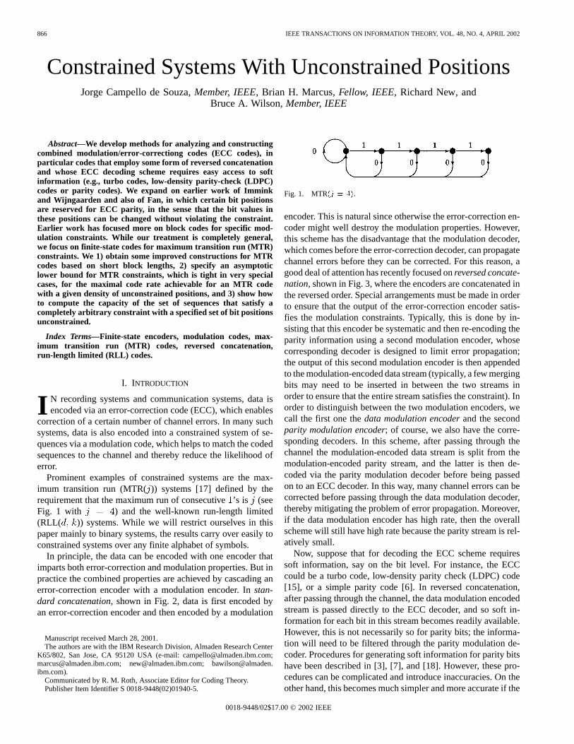
Prominent examples of constrained systems are the max-imum transition run (MTR()) systems [17] defined by therequirement that the maximum run of consecutive’s is (seeFig. 1 with ) and the well-known run-length limited(RLL( )) systems. While we will restrict ourselves in thispaper mainly to binary systems, the results carry over easily toconstrained systems over any finite alphabet of symbols.

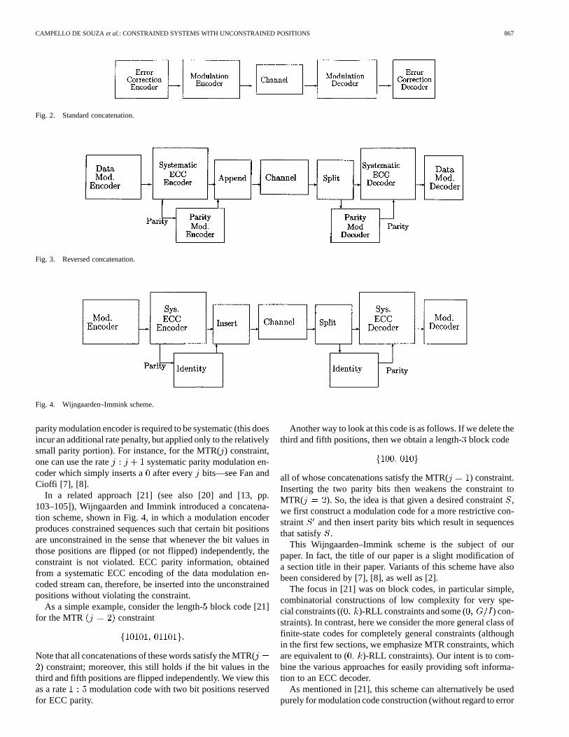
In principle, the data can be encoded with one encoder thatimparts both error-correction and modulation properties. But inpractice the combined properties are achieved by cascading anerror-correction encoder with a modulation encoder. Instan-dard concatenation, shown in Fig. 2, data is first encoded byan error-correction encoder and then encoded by a modulation

Manuscript received March 28, 2001.The authors are with the IBM Research Division, Almaden Research Center

K65/802, San Jose, CA 95120 USA (e-mail: [email protected];[email protected]; [email protected]; [email protected]).

Communicated by R. M. Roth, Associate Editor for Coding Theory.Publisher Item Identifier S 0018-9448(02)01940-5.

Fig. 1. MTR(j = 4).

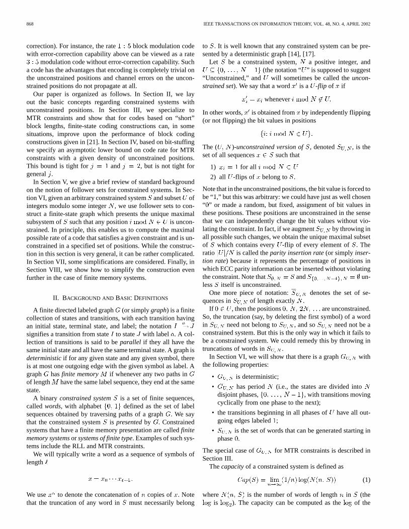
encoder. This is natural since otherwise the error-correction en-coder might well destroy the modulation properties. However,this scheme has the disadvantage that the modulation decoder,which comes before the error-correction decoder, can propagatechannel errors before they can be corrected. For this reason, agood deal of attention has recently focused onreversed concate-nation, shown in Fig. 3, where the encoders are concatenated inthe reversed order. Special arrangements must be made in orderto ensure that the output of the error-correction encoder satis-fies the modulation constraints. Typically, this is done by in-sisting that this encoder be systematic and then re-encoding theparity information using a second modulation encoder, whosecorresponding decoder is designed to limit error propagation;the output of this second modulation encoder is then appendedto the modulation-encoded data stream (typically, a few mergingbits may need to be inserted in between the two streams inorder to ensure that the entire stream satisfies the constraint). Inorder to distinguish between the two modulation encoders, wecall the first one thedata modulation encoderand the secondparity modulation encoder; of course, we also have the corre-sponding decoders. In this scheme, after passing through thechannel the modulation-encoded data stream is split from themodulation-encoded parity stream, and the latter is then de-coded via the parity modulation decoder before being passedon to an ECC decoder. In this way, many channel errors can becorrected before passing through the data modulation decoder,thereby mitigating the problem of error propagation. Moreover,if the data modulation encoder has high rate, then the overallscheme will still have high rate because the parity stream is rel-atively small.

Now, suppose that for decoding the ECC scheme requiressoft information, say on the bit level. For instance, the ECCcould be a turbo code, low-density parity check (LDPC) code[15], or a simple parity code [6]. In reversed concatenation,after passing through the channel, the data modulation encodedstream is passed directly to the ECC decoder, and so soft in-formation for each bit in this stream becomes readily available.However, this is not necessarily so for parity bits; the informa-tion will need to be filtered through the parity modulation de-coder. Procedures for generating soft information for parity bitshave been described in [3], [7], and [18]. However, these pro-cedures can be complicated and introduce inaccuracies. On theother hand, this becomes much simpler and more accurate if the

0018-9448/02$17.00 © 2002 IEEE

CAMPELLO DE SOUZAet al.: CONSTRAINED SYSTEMS WITH UNCONSTRAINED POSITIONS 867

Fig. 2. Standard concatenation.

Fig. 3. Reversed concatenation.

Fig. 4. Wijngaarden–Immink scheme.

parity modulation encoder is required to be systematic (this doesincur an additional rate penalty, but applied only to the relativelysmall parity portion). For instance, for the MTR() constraint,one can use the rate systematic parity modulation en-coder which simply inserts aafter every bits—see Fan andCioffi [7], [8].

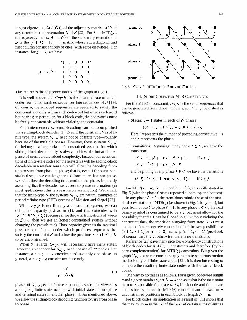
In a related approach [21] (see also [20] and [13, pp.103–105]), Wijngaarden and Immink introduced a concatena-tion scheme, shown in Fig. 4, in which a modulation encoderproduces constrained sequences such that certain bit positionsare unconstrained in the sense that whenever the bit values inthose positions are flipped (or not flipped) independently, theconstraint is not violated. ECC parity information, obtainedfrom a systematic ECC encoding of the data modulation en-coded stream can, therefore, be inserted into the unconstrainedpositions without violating the constraint.

As a simple example, consider the length-block code [21]for the MTR constraint

Note that all concatenations of these words satisfy the MTR() constraint; moreover, this still holds if the bit values in the

third and fifth positions are flipped independently. We view thisas a rate modulation code with two bit positions reservedfor ECC parity.

Another way to look at this code is as follows. If we delete thethird and fifth positions, then we obtain a length-block code

all of whose concatenations satisfy the MTR( ) constraint.Inserting the two parity bits then weakens the constraint toMTR( ). So, the idea is that given a desired constraint,we first construct a modulation code for a more restrictive con-straint and then insert parity bits which result in sequencesthat satisfy .

This Wijngaarden–Immink scheme is the subject of ourpaper. In fact, the title of our paper is a slight modification ofa section title in their paper. Variants of this scheme have alsobeen considered by [7], [8], as well as [2].

The focus in [21] was on block codes, in particular simple,combinatorial constructions of low complexity for very spe-cial constraints (( )-RLL constraints and some ( ) con-straints). In contrast, here we consider the more general class offinite-state codes for completely general constraints (althoughin the first few sections, we emphasize MTR constraints, whichare equivalent to ( )-RLL constraints). Our intent is to com-bine the various approaches for easily providing soft informa-tion to an ECC decoder.

As mentioned in [21], this scheme can alternatively be usedpurely for modulation code construction (without regard to error


correction). For instance, the rate block modulation codewith error-correction capability above can be viewed as a rate

modulation code without error-correction capability. Sucha code has the advantages that encoding is completely trivial onthe unconstrained positions and channel errors on the uncon-strained positions do not propagate at all.

Our paper is organized as follows. In Section II, we layout the basic concepts regarding constrained systems withunconstrained positions. In Section III, we specialize toMTR constraints and show that for codes based on “short”block lengths, finite-state coding constructions can, in somesituations, improve upon the performance of block codingconstructions given in [21]. In Section IV, based on bit-stuffingwe specify an asymptotic lower bound on code rate for MTRconstraints with a given density of unconstrained positions.This bound is tight for and , but is not tight forgeneral .

In Section V, we give a brief review of standard backgroundon the notion of follower sets for constrained systems. In Sec-tion VI, given an arbitrary constrained systemand subset ofintegers modulo some integer, we use follower sets to con-struct a finite-state graph which presents the unique maximalsubsystem of such that any position is uncon-strained. In principle, this enables us to compute the maximalpossible rate of a code that satisfies a given constraint and is un-constrained in a specified set of positions. While the construc-tion in this section is very general, it can be rather complicated.In Section VII, some simplifications are considered. Finally, inSection VIII, we show how to simplify the construction evenfurther in the case of finite memory systems.

II. BACKGROUND AND BASIC DEFINITIONS

A finite directed labeled graph (or simplygraph) is a finitecollection of states and transitions, with each transition havingan initial state, terminal state, and label; the notationsignifies a transition from stateto state with label . A col-lection of transitions is said to beparallel if they all have thesame initial state and all have the same terminal state. A graph isdeterministicif for any given state and any given symbol, thereis at most one outgoing edge with the given symbol as label. Agraph hasfinite memory if whenever any two paths inof length have the same label sequence, they end at the samestate.

A binary constrained system is a set of finite sequences,calledwords, with alphabet defined as the set of labelsequences obtained by traversing paths of a graph. We saythat the constrained systemis presentedby . Constrainedsystems that have a finite memory presentation are calledfinitememory systemsor systems of finite type. Examples of such sys-tems include the RLL and MTR constraints.

We will typically write a word as a sequence of symbols oflength

We use to denote the concatenation ofcopies of . Notethat the truncation of any word in must necessarily belong

to . It is well known that any constrained system can be pre-sented by a deterministic graph [14], [17].

Let be a constrained system, a positive integer, and(the notation “ ” is supposed to suggest

“Unconstrained,” and will sometimes be called theuncon-strained set). We say that a word is a -flip of if

whenever

In other words, is obtained from by independently flipping(or not flipping) the bit values in positions

The ( )-unconstrained version of , denoted , is theset of all sequences such that

1) for all

2) all -flips of belong to .

Note that in the unconstrained positions, the bit value is forced tobe “ ,” but this was arbitrary: we could have just as well chosen“ ” or made a random, but fixed, assignment of bit values inthese positions. These positions are unconstrained in the sensethat we can independently change the bit values without vio-lating the constraint. In fact, if we augment by throwing inall possible such changes, we obtain the unique maximal subsetof which contains every -flip of every element of . Theratio is called theparity insertion rate(or simply inser-tion rate) because it represents the percentage of positions inwhich ECC parity information can be inserted without violatingthe constraint. Note that and un-less itself is unconstrained.

One more piece of notation: denotes the set of se-quences in of length exactly .

If , then the positions are unconstrained.So, the truncation (say, by deleting the first symbol) of a wordin need not belong to , and so need not be aconstrained system. But this is the only way in which it fails tobe a constrained system. We could remedy this by throwing intruncations of words in .

In Section VI, we will show that there is a graph withthe following properties:

• is deterministic;

• has period (i.e., the states are divided intodisjoint phases, , with transitions movingcyclically from one phase to the next);

• the transitions beginning in all phases ofhave all out-going edges labeled;

• is the set of words that can be generated starting inphase .

The special case of for MTR constraints is described inSection III.

Thecapacityof a constrained system is defined as

Cap (1)

where is the number of words of length in (theis ). The capacity can be computed as the of the


largest eigenvalue, , of the adjacency matrix ofany deterministic presentation of [22]. For MTR ,the adjacency matrix of the standard presentation of

is the matrix whose superdiagonal andfirst column consist entirely of ones (with zeros elsewhere). Forinstance, for , we have

This matrix is the adjacency matrix of the graph in Fig. 1.

It is well known thatCap is the maximal rate of an en-coder from unconstrained sequences into sequences of[19].Of course, the encoded sequences are required to satisfy theconstraint, not only within each codeword but across codewordboundaries; in particular, for a block code, the codewords mustbe freely concatenable without violating the constraint.

For finite-memory systems, decoding can be accomplishedvia a sliding-block decoder [1]. Even if the constraintis of fi-nite type, the system need not be of finite type—roughlybecause of the multiple phases. However, these systemsdo belong to a larger class of constrained systems for whichsliding-block decodability is always achievable, but at the ex-pense of considerable added complexity. Instead, our construc-tions of finite-state codes for these systems will be sliding-blockdecodable in a weaker sense: we will allow the decoding func-tion to vary from phase to phase; that is, even if the same con-strained sequence can be generated from more than one phase,we will allow the decoding to depend on the phase, implicitlyassuming that the decoder has access to phase information (inmost applications, this is a reasonable assumption). We remarkthat for finite-type , the systems are natural examples ofperiodic finite type (PFT) systems of Moision and Siegel [23]

While is not literally a constrained system, we candefine its capacity just as in (1), and this coincides with

(because if we throw in truncations of wordsin , then we get an honest constrained system withoutchanging the growth rate). Thus, capacity gives us the maximalpossible rate of an encoder which produces sequences thatsatisfy the constraint and allow the positionsto be unconstrained.

When is large, will necessarily have many states.However, an encoder for need not use all phases. Forinstance, a rate encoder need use only one phase. Ingeneral, a rate encoder need use only

(2)

phases of ; each of these encoder phases can be viewed asa rate finite-state machine with initial states in one phaseand terminal states in another phase [4]. As mentioned above,we allow the sliding-block decoding function to vary from phaseto phase.

Fig. 5. G for MTR(j = 4),N = 3 andU = f1g.

III. SHORT CODES FORMTR CONSTRAINTS

For the MTR( ) constraint, is the set of sequences thatcan be generated from phasein the graph , described asfollows.

• States: states in each of phases

Here represents the number of preceding consecutive’sand represents the phase.

• Transitions: Beginning in any phase , we have thetransitions

if

and beginning in any phase we have the transitions

if

For MTR( ), , and , this is illustrated inFig. 5 (with the phase states repeated at both top and bottom).

In any phase , the transitions mimic those of the stan-dard presentation of MTR() (as shown in Fig. 1 for ), butpass from phaseto phase . In any phase , the nextbinary symbol is constrained to be a, but must allow for thepossibility that the can be flipped to a without violating theconstraint; thus, the transition outgoing from state mustend at the “more severely constrained” of the two possibilities:

or , namely, (provided,of course, that ; otherwise, there is no transition).

Reference [21] gave many nice low-complexity constructionsof block codes for RLL( ) constraints and therefore (by bi-nary complementation) for MTR() constraints. But given thegraph , one can consider applying finite-state constructionmethods to yield finite-state codes [22]. It is then interesting tocompare the resulting finite-state codes with the earlier blockcodes.

One way to do this is as follows. For a given codeword lengthand a given number, set and ask what is the maximum

number possible for a rate block code and finite-statecode which satisfies the MTR() constraint and allows forunconstrained positions in each block of length .

For block codes, an application of a result of [11] shows thatthe maximum is the of the of certain sums of entries


TABLE IFOR MTR(j = 3), MAXIMUM NUMBER m OF INFORMATION BITS FORGIVEN

LENGTH q = N AND NUMBER u OF UNCONSTRAINEDPOSITIONS

of powers of the adjacency matrix: for MTR( ), this turnsout to be the of the of the four quantities

where is the adjacency matrix of and the indicesof refer to states and in .

For finite-state codes, an application of [1] shows that themaximum is .

Table I reveals that, for MTR( ) and some choices ofand , the number can be increased if

one allows a finite-state code rather than a block code (see thebold-faced entries in the table). The column labeled “window”shows the length, measured in number of-blocks, of the de-coder window for the finite-state code (of course, the decoderwindow for a block code is always). The column labeled “#states” shows the number of encoder states for the finite-statecode (of course, a block code has only one state). The entries inthese columns are determined by finding an approximate eigen-vector and corresponding state splitting [22].

One can then evaluate tradeoffs between the block codes andfinite-state codes. For instance, the rate block code with

can be compared against the rate finite-statecode with . Here, the finite-state code has twice the errorcorrection power of the block code, but the former has to copewith some error propagation. For bursty channels, the finite-state code would probably perform better.

One can also compare the rate block code againstthe rate finite-state code, each with . Here, theblock code will have better error protection (one parity bit per10 bits versus one parity bit per 11 bits) and will not have tocope with error propagation, but the finite-state code will havea higher rate. In a low-SNR regime, the block code may be su-perior, while in a high-SNR regime the finite-state code may besuperior.

The entries in the table indicate that even the finite-state codesare not terribly complex. But in general they will not match the

TABLE IIRATE 8=9 CODES FORMTR(j = 4)

very low complexity of the Wjingaarden–Immink constructions[21].

For the codes in Table I, the codeword lengthcoincides withthe in the definition of , and so the parity insertion rateis always . According to the discussion at the end ofSection II, this has the advantage that only one of thephasesneed be used in the construction of an encoder. On the otherhand, in this case, we must have , for otherwise wewould have a rate encoder that satisfies the constraint. Inparticular, if , we can never have a rate code(indeed, this is consistent with the results in the table). On theother hand, if we allow the possibility of it is possible toconstruct codes with rate and .

For this purpose, we now consider the constraintMTR (a “reasonably well-constrained” system forrecording applications), and we compare codes at rate(a“reasonably high” rate for combined modulation and ECC ina recording application), but allowing for the possibility of

.Table II presents a list of four rate codes for MTR( ).

The first code is a block code with the shortest block lengththat permits a nonzero parity insertion rate and code rate at

least . Here, and the parity insertion rateis (the encoder operates at rate ). Itturns out that if one wants to strictly increase the insertion rate,but still keep the code rate at least , then for a block code,the block length must increase to . For this code,one can arrange for and so the insertion rate is

. However, the large block length means thatencoding is probably very complex. On the other hand, the samecode rate ( ) and insertion rate ( ) can be achieved via afinite-state code (code #3) with block length only (here,

and ). Moreover, the decoder window has lengthtwo 9-bit blocks, and so is comparable (in number of bits) to

code #1 (and much shorter than that of code #2). Also, accordingto (2) only five of the 15 phases need be used for an encoder,and it turns out that such an encoder can be constructed withroughly five states per phase. Finally, code #4 again has blocklength , code rate , and further improved insertionrate . But this code probably requires a largerdecoding window (three 9-bit blocks).

Actually, for MTR( ), one can computeCap. This suggests trying for a rate modulation code

with parity insertion rate —thereby improving the rate( ) of code #3 above. Moreover, according to (2), the encoderneed use only


of the 15 phases of ; however, estimates using an ap-proximate eigenvector [22] show that such an encoder will havean average of at least 37 states per phase, yielding a total of atleast 100 encoder states (and possibly many more).

Of course, everything we have done in this section for MTRconstraints applies equally well to -RLL constraints viabinary complementation.

IV. L ONG CODES FORMTR CONSTRAINTS

In Section III, we considered codes for MTR constraintsbased on relatively short block lengths. For instance, forMTR( ) and code rate , we found a code with parityinsertion rate approximately . The encoder had blocklength and the decoder had a window of at most 27bits. We can improve upon the insertion rate, at the expenseof increasing the block length, by the following construction,essentially due to [7], [9].

For , we say that a string is a-bit-stuffing-MTR( )string if it is obtained as follows: begin with a stringthat satis-fies the MTR( ) constraint and subdivideinto intervals ofsize ; then, in between each of these intervals insert astring of ones. The resulting string satisfies the MTR() con-straint and has parity insertion rate . The set of all suchstrings of a fixed length can be viewed as a block code, andthe asymptotic optimal code rate of such codes, as , is

(where denotes the largest eigenvalue of thestandard adjacency matrix for the MTR( ) constraint). Ofcourse, if we want to ensure that free concatenations of code-words also satisfy the constraint, then we must add a “” bit atthe end of the entire string.

If the desired insertion rate is not a multiple of , wecan construct a code via a weighted average of two bit-stuffingschemes: if , consider a weighted average of

-bit-stuffing-MTR( ) and -bit-stuffing-MTR( ): subdi-vide an interval of some large lengthinto two subintervals anddo -bit-stuffing in the first subinterval and -bit-stuffingin the second subinterval; the subintervals should have lengths

and , where

(3)

Note that the asymptotic optimal code rate of such block codesis

(4)

Again, in order to ensure that the resulting strings satisfy theMTR( ) constraint, we need to insert a “” bit in between thetwo subintervals.

For MTR( ), the parity insertion rate lies inbetween and . Thus, this insertion rate canbe realized via a weighted average of-bit-stuffing and -bit-stuffing with weight (according to(3) with ). This yields an asymptotic code rate, as in (4),of approximately

Thus, the code rate can be achieved with insertion ratestrictly larger than . Indeed, setting (4) equal to ,

solving for , and then solving for in (3), we get ;so we can achieve code rate with insertion rate as high as

.For MTR and parity insertion rate, let denote

the code rate obtained by the weighted average of-bit-stuffingand -bit-stuffing, described above. According to (4), thegraph of is the piecewise-linear curve that connects the

points

•

•

•

•

•

• .

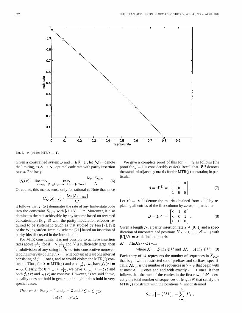
This is illustrated in Fig. 6 for . Each point where theslope changes is indicated by an “.” The point plotted as “o”is , indicating that a weighted average of twobit-stuffing schemes can achieve code rate with insertionrate approximately (as mentioned above).

One might imagine achieving still higher rates by using aweighted average of more than two of the bit-stuffing schemesmentioned above. However, Fig. 6 suggests that is con-cave, and so this would not yield any improvement. Indeed, thisis the case.

Proposition 1: For all positive integers, the functionis concave on the domain (in fact, strictly concave onthe domain of points ). Thus, for parity in-sertion rate with , the weighted average of

-bit-stuffing-MTR( ) and -bit-stuffing-MTR( ) yieldsa strictly higher code rate than any other weighted average ofbit stuffings.

Proof: Since concavity is not affected by an affine changeof the independent variable, the proposition is equivalent to thefollowing lemma, which we prove in the Appendix.

Lemma 2: The function

(5)

is strictly concave on the domain of positive integers.

At this point, it is natural to ask if weighted averages of thesebit-stuffing schemes are optimal, i.e., if is the asymptoticoptimal rate of codes that satisfy the constraint MTRfor a given insertion rate . This turns out to be true for veryspecial cases (see Theorem 3 later). However, it is false in gen-eral. For example, for MTR , and

(and so ), it turns out thatCap , yet . We leave, asan open problem, the question of whether or not there is a largerclass of simple bit-stuffing schemes that completely describe theoptimal coding schemes (for all).

We pause to put this in a more formal setting. Recall thatdenotes the set of sequences in of length exactly .


Fig. 6. g (x) for MTR(j = 4).

Given a constrained systemand , let denotethe limiting, as , optimal code rate with parity insertionrate . Precisely

(6)

Of course, this makes sense only for rational. Note that since

Cap

it follows that dominates the rate of any finite-state codeinto the constraint with . Moreover, it alsodominates the rate achievable by any scheme based on reversedconcatenation (Fig. 3) with the parity modulation encoder re-quired to be systematic (such as that studied by Fan [7], [9])or the Wijngaarden–Immink scheme [21] based on insertion ofparity bits discussed in the Introduction.

For MTR constraints, it is not possible to achieve insertionrates above : for if and is sufficiently large, thena subdivision of any string in into consecutive nonover-lapping intervals of length will contain at least one intervalconsisting of ones, and so would violate the MTR() con-straint. Thus, for MTR and , we have

. Clearly, for , we have andboth and are concave. However, as we said above,equality does not hold in general, although it does hold in veryspecial cases.

Theorem 3: For and and

We give a complete proof of this for as follows (theproof for is considerably easier). Recall that denotesthe standard adjacency matrix for the MTR() constraint; in par-ticular

(7)

Let denote the matrix obtained from by re-placing all entries of the first column by zeros; in particular

(8)

Given a length , a parity insertion rate and a spec-ification of unconstrained positions with

, define the matrix

where if and if (9)

Each entry of represents the number of sequences inthat begin with a restricted set of prefixes and suffixes; specifi-cally, is the number of sequences in that begin withat most ones and end with exactly ones. It thenfollows that the sum of the entries in the first row of is ex-actly the total number of sequences of lengththat satisfy theMTR( ) constraint with the positions unconstrained


(here, denotes the column vector consisting entirely of ones).The crux of our proof of Theorem 3 is the following lemma,which is proved in the Appendix.

Lemma 4: There is a fixed constant satisfying the fol-lowing. Given a length , a parity insertion rate anda specification of unconstrained positionswith , let be the matrix defined in (9). Then thereis a matrix of the form

(10)

such that

1) ,

2) the number of occurrences of in (10) is within of, and

3) the number of occurrences of in (10) is within of.

Proof of Theorem 3 for : It follows from Lemma 4(part 1) and Perron–Frobenius Theory [14, Ch. 4] that, up to afixed multiplicative constant, is dominated by

where , , and are the largest eigenvalues of , ,and , respectively. We claim that

(recall that denotes the largest eigenvalue of the adjacencymatrix ). This follows by straightforward computation (infact, more generally, for arbitraryand , one can usethe recurrence relation to showthat is a block triangular matrix withdiagonal blocks and , and so indeed ).So, up to a fixed multiplicative constant, is dominated by

Let

Then is dominated by a weighted average of the num-bers

with weights

These same weights applied to the numbersyield

(11)

According to Lemma 4 (parts 2 and 3), the numerator (respec-tively, denominator) of the right-hand side of (11) differs from

(respectively, ) by at most (respectively, ). Thus,as , the right-hand side of (11) tends to. Sinceis continuous and concave (Proposition 1), is dominatedby (and hence equal to) .

V. FOLLOWER SETS OFCONSTRAINED SYSTEMS

In this section, we briefly summarize some background onfollower sets for constrained systems. For a more thorough treat-ment, the reader may consult [14] or [22].

Given a set of finite sequences and a finite sequence, thefollower setof is defined as follows:

finite sequences

We allow to be the empty word, in which case the followerset is all of . Note that if does not occur in , then isempty. Any constrained system has only finitely many followersets [14], [22].

Since a constrained system typically has infinitely manywords, many follower sets must coincide with one another. Forexample, for the constrained system MTR() the follower set ofa word depends only on its suffix of length; in fact, this systemhas only follower sets: .The follower sets can be used to manufacture a special presen-tation , called thefollower set graph,of a constrained system

. Namely, the states of are follower sets and the transitionsare

(12)

provided that occurs in . Note in particular that the followerset graph is deterministic. Note also that whenever a wordisthe label of a path in the follower set graph ending at state ,we must have .

Some follower sets are helpful for proofs but not so much forcode construction. Clearly, the follower set of the empty wordis an example—more generally, so is any follower set that hasno incoming edges or no outgoing edges.

An irreducible graph is a graph such that for any givenordered pair of states there is a path in the graph from

to . Any graph can be decomposed into irreducible sub-graphs (calledirreducible components) together with transientconnections from one component to another. Anirreducibleconstrained systemis a constrained system such that for anygiven ordered pair of words and in , there is a wordsuch that is also in . It turns out that any irreducible con-strained system can be presented by an irreducible componentof its follower set graph; this component is sometimes calledthe irreducible follower set graph[14].

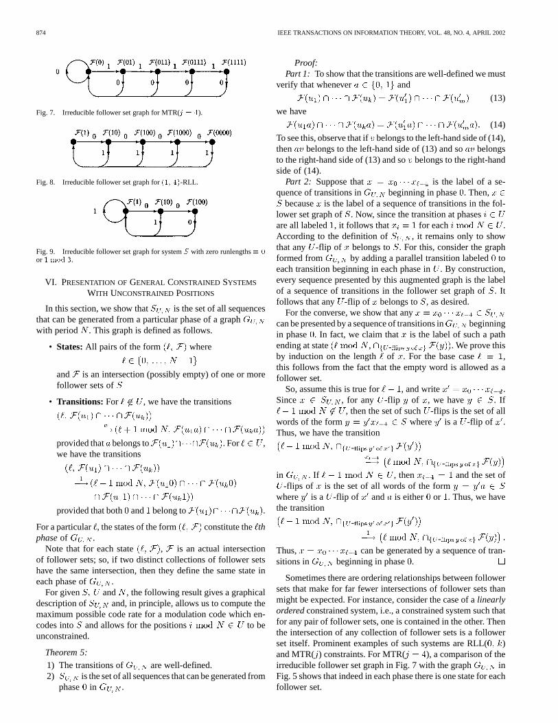
Most constrained systems of interest are irreducible. For in-stance, the irreducible follower set graphs of some MTR andRLL constraints are given in Fig. 7 and 8. These agree withthe standard presentations that are usually given for these con-straints (in particular, Figs. 1 and 7 agree).

Sometimes the irreducible follower set graph agrees with thefollower set graph itself (for instance, for MTR constraints),and sometimes the irreducible follower set graph is obtained bymerely deleting the follower set of the empty word (for instance,for RLL constraints). But quite often more follower sets need tobe deleted.

As another example, Fig. 9 shows the irreducible followerset graph for the constrained system, defined by requiring thatrunlengths of zeros be congruent to eitheror modulo .


Fig. 7. Irreducible follower set graph for MTR(j = 4).

Fig. 8. Irreducible follower set graph for(1; 4)-RLL.

Fig. 9. Irreducible follower set graph for systemS with zero runlengths= 0or 1 mod 3.

VI. PRESENTATION OFGENERAL CONSTRAINED SYSTEMS

WITH UNCONSTRAINEDPOSITIONS

In this section, we show that is the set of all sequencesthat can be generated from a particular phase of a graphwith period . This graph is defined as follows.

• States:All pairs of the form where

and is an intersection (possibly empty) of one or morefollower sets of

• Transitions: For , we have the transitions

provided that belongs to . For ,we have the transitions

provided that both and belong to .

For a particular , the states of the form constitute thethphaseof .

Note that for each state , is an actual intersectionof follower sets; so, if two distinct collections of follower setshave the same intersection, then they define the same state ineach phase of .

For given and , the following result gives a graphicaldescription of and, in principle, allows us to compute themaximum possible code rate for a modulation code which en-codes into and allows for the positions to beunconstrained.

Theorem 5:

1) The transitions of are well-defined.2) is the set of all sequences that can be generated from

phase in .

Proof:Part 1: To show that the transitions are well-defined we must

verify that whenever and

(13)

we have

(14)

To see this, observe that ifbelongs to the left-hand side of (14),then belongs to the left-hand side of (13) and sobelongsto the right-hand side of (13) and sobelongs to the right-handside of (14).

Part 2: Suppose that is the label of a se-quence of transitions in beginning in phase. Then,

because is the label of a sequence of transitions in the fol-lower set graph of . Now, since the transition at phasesare all labeled , it follows that for each .According to the definition of , it remains only to showthat any -flip of belongs to . For this, consider the graphformed from by adding a parallel transition labeledtoeach transition beginning in each phase in. By construction,every sequence presented by this augmented graph is the labelof a sequence of transitions in the follower set graph of. Itfollows that any -flip of belongs to , as desired.

For the converse, we show that anycan be presented by a sequence of transitions in beginningin phase . In fact, we claim that is the label of such a pathending at state , - . We prove thisby induction on the length of . For the base case ,this follows from the fact that the empty word is allowed as afollower set.

So, assume this is true for , and write .Since , for any -flip of , we have . If

, then the set of such -flips is the set of allwords of the form where is a -flip of .Thus, we have the transition

-

-in . If , then and the set of

-flips of is the set of all words of the formwhere is a -flip of and is either or . Thus, we havethe transition

-

-Thus, can be generated by a sequence of tran-sitions in beginning in phase.

Sometimes there are ordering relationships between followersets that make for far fewer intersections of follower sets thanmight be expected. For instance, consider the case of alinearlyorderedconstrained system, i.e., a constrained system such thatfor any pair of follower sets, one is contained in the other. Thenthe intersection of any collection of follower sets is a followerset itself. Prominent examples of such systems are RLL()and MTR( ) constraints. For MTR( ), a comparison of theirreducible follower set graph in Fig. 7 with the graph inFig. 5 shows that indeed in each phase there is one state for eachfollower set.


Finally, recall that denotes the set of all sequences ofpaths of length in , and so is the set of all label se-quences of paths in that begin at . It follows thatthe size of this set can, in principle, be computed fromthe adjacency matrix of . Note thatis the maximal rate at which we can encode into sequences oflength such that

1) all codewords obey the constraint(although concatena-tions of codewords need not obey the constraint);

2) for any codeword the bit value in any position is1 but can be freely switched to 0 without violating theconstraint .

VII. SIMPLIFICATIONS

The graph may be enormous relative to, even forsmall . However, the number of states can be reduced in thefollowing steps.

Step 1: Not all intersections of follower sets are needed at allphases. Rather, we need only a collection of intersections that isclosed under the following operations:

• for

• for

and

(of course, we need only those above that define valid tran-sitions in ).

So, starting only with follower sets (but not intersections offollower sets) in phase 0, we can accumulate, cyclically fromphase to phase, only those states obtained from applying theseoperations, until no new states occur; of course, we may have totraverse each phase several times until the process stops. Thisgenerally results in far fewer states.

Step 2: Even after Step 1, we still may be left withinessentialstates, i.e., states which are either not the terminal state or initialstate of arbitrarily long words (in particular, we can delete statesof the form where is either empty or the follower setof the empty word). For example, in the graph of Fig. 5, theinessential states are the second and fifth states in phase 0, thethird and fifth states in phase 1, and the first and fourth states inphase 2.

As another example, consider the systemshown in Fig. 9,with and . In phase 0, all outgoing edges

Fig. 10. Presentation ofS for system S with zero runlengths= 0; 1mod 3.

must be labeled “.” But since “ ” cannot follow “ ,” for any, the state has no outgoing edges and is

therefore inessential. But this forces other states in phase 0 tobe inessential. For example, we can easily check that the onlypath outgoing from the state is as shownin the expression at the bottom of the page. Since the terminalstate of this path is inessential, each state in this path, in partic-ular , must be inessential. In fact, it turns outthat all that remains after deleting inessential states is shown inFig. 10.

Step 3: Third, even if is irreducible, it still can happen thatthe graph resulting from Steps 1 and 2 is reducible. However,there is always at least one irreducible component of maximalcapacity. For coding purposes, we can delete all but one suchcomponent.

VIII. F INITE-MEMORY SYSTEMS

Recall that a presentation of a constrained system hasfinite memory if whenever any two paths in of lengthhave the same label sequence, they end at the same state; andconstrained systems that have a finite memory presentation arecalled finite-memory systems. For such a system, the followerset graph always has finite memory; in fact, the follower set ofany word of length equals the follower set of its suffixof length . Prominent examples of finite-memory systemsare RLL, MTR systems, and their NRZ precoded versions. Thesystem in Fig. 9 and the well-known charge-constrained systemsdo not have finite memory. The following result shows how thegraph can be simplified for finite-memory systems.

Theorem 6: Let be an irreducible constrained system offinite memory and an and satisfying the

Gap Condition:the gaps (modulo ) between elementsof are all of size at least .

Then the Procedure given in Step 1 of Section VII results instates of the form where is either asingleton, i.e., asingle follower set or adoubleton, i.e., an intersection of exactlytwo follower sets. Moreover, the only phasesfor which a state

can be a doubleton are those where ,where and .

Proof: Without loss of generality, we can assume that. First observe that, applying the procedure in Step 1, we begin


Fig. 11. Presentation ofS for S = (1; 4)-RLL.

with singletons in phase 0, and because of the Gap Condition,we accumulate only (at worst) doubletons in phases .In particular, any state accumulated in phasewill be of theform for some word of length . Butby definition of finite memory, ,and so in phase , these are really singletons. They will remainsingletons in phases until the next phase

is encountered; from then on, we will see only(at worst) doubletons for at most more phases, againbecause of the Gap Condition. But in the next phase, the finitememory condition will force singletons, etc.

As an example, consider, the -RLL system, withand . Beginning with the irreducible follower set

graph in Fig. 8, we apply the constructions of Theorems 5 and6. We claim that after eliminating inessential states, we are leftwith the graph, shown in Fig. 11, which presents . To seethis, first observe that for any word, the state willhave an outgoing edge in only if both and belong to

. This eliminates the states and . Forstate , there is an outgoing transition, labeledtostate , but neither nor can be generatedfrom this state. So, the only surviving states in phaseare

andBy starting from these states, and applying the Procedure inStep 1, one can check that all that remains of is that shownin Fig. 11.

Now, note that in this graph there are exactly three paths oflength from phase 0 to itself, one from each ofto , to

, and to . It follows thatCap whereis the largest eigenvalue of the matrix

It is well-known that and .So,Cap .

Further simplifications are possible if we are willing to com-bine some phases together. This will be useful for simplifyingthe capacity computation and for constructing rate codesin the case where is a multiple of . We need the followingformal constructions to do this.

1) Let be a graph and a positive integer. Thehigherpower graph is the graph with the same state set as

, and an edge labeled by a sequence of lengthfor eachpath in of length (with the label inherited from thepath).

2) For a graph and an integer , let denote thegraph with states in and the following transitions:whenever there are two paths from stateto state ,one with label and the other with label

, endow with a transition from toand label .

3) For graphs , each with the same setof states, let denote the graph

(“trellis construction”) defined by the following.

• States:The union of disjoint copies,, of .

• Transitions: For each mimiceach transition in , with a transition from to

(where the subscripts are read modulo).

Now, let be an irreducible constrained system with memorypresented by its irreducible follower set graph. Assume

the Gap Condition and that . Write the unconstrained setand write . From Theorem 6,

we see that is the set of sequences generated by


beginning in . The adjacency matrix of the higher powergraph restricted to phase 0 is

where is the adjacency matrix of , and is the adjacencymatrix of . Thus, the capacity of can then be computedas where is the largest eigenvalue of. Notethat in the special case , this reduces to

As an example, consider again for -RLL.Here

The graph has memory and one can check that the graphhas only three edges: , ,

and , and so

We compute

the essential part of which is simply the submatrix deter-mined by the second and third rows and columns

consistent with the computation earlier in this section.

APPENDIX

PROOFS OFLEMMAS 2 AND 4

Proof of Lemma 2:It is well known [13, p. 61] that is theunique solution to the equation

Let be a real variable. We claim that for each value of ,the equation

(15)

has a unique solution . This is a consequenceof the following facts regarding the left-hand side of (15):

• it is at ,

• it is at ,

• it has negative derivative (as a function of) at(namely, the derivative is ),

• it has derivative at only one point (namely, at).

In particular, note that

(16)

We claim that and so is monotonically in-creasing with . To see this, first rewrite (15) as ,take natural logs and differentiatewith respect to to obtain

equivalently

which is positive by (16).For , let

Note that and so is increasing with . It sufficesto show that on the domain . We find it easierinstead to show that merely for all and thenuse an auxiliary argument to complete the proof of concavity ofthe function (5) on the domain of positive integers.

For this, first note that . It follows thatsatisfies the equation

which we can rewrite as

(17)

In what follows, we will write as simply. Differentiating (17) with respect to, we obtain

Solving for , we obtain

Now, substituting for via (17), we obtain

Multiplying numerator and denominator by, we obtain

(18)

Differentiating this equation with respect to, we see that

where is positive

and .We will show that for all . Now, using (18), we

substitute for only in the second factor of the first term ofand obtain


But this expression simplifies to

Thus, if and only if

(19)

Now, we can rewrite (18) as

So, the inequality (19) is equivalent to

Recalling that , it follows from (18) that ,and so the preceding inequality is equivalent to

(20)

For , one computes that

Now, since is increasing with , we have for all; thus, (20) holds for . Thus, the function (5) is

concave on the domain of integers . Now, one can verify,via explicit computation, that this function is concave on thedomain of integers . Since the domain of positiveintegers is the union of these two domains, which intersect intwo consecutive integers (namely, ), it follows that thefunction (5) is concave on the entire domain of positive integers,as desired (use the characterization of a concave function as afunction with decreasing slopes).

Proof of Lemma 4:Let and be as in (7) and (8). We willmake use of the following matrix relations:

R1: ;

R2: ;

R3: for all ;

R4: for all;

R5: for all

The first three of these relations can be verified by straightfor-ward computation. The fourth and fifth, which we verify below,are a bit more subtle.

We will use these relations to gradually transforminto thedesired form .

It follows from R1 that we may assume in (9) that we neversee three consecutive’s.

Stage 1: From R2, we see that we can delete each appearanceof without decreasing any entry of (we can assume in(9) that ends with an ). But in the course of doing so, wechange the length and insertion rate. We will rectify this ina moment; but for now, simply let denote the total numberof occurrences of that we have deleted in this stage.

Stage 2: At this point, we may assume that contains onlyisolated copies of . It follows from R3 that we can replace anyoccurrence of with and not changeany entry of (again, this changes the lengthand insertionrate ). Let denote the total number of occurrences of

that we have deleted in Stage 2. Then, tack on to the right endof the matrix

This will not decrease . Note that if were divisible by ,then this would completely rectify the length and insertion rate.Otherwise, it changes, in (9), the number of occurrences ofand the number of occurrences ofby bounded amounts.

Stage 3: Now is a product of several intermingled powersof , , and isolated copies of , followed by a singlepower of and a single power of . Using R4, we cancombine each isolated copy of with an to form anothercopy of . Then, using R5, we can combine all powers oftogether and all powers of together, yielding a matrix ofthe form

Then we can delete some initial copies ofto make divisibleby at the expense of changing the number of occurrences of

by a bounded amount. This completes the proof of Lemma 4,except for the verification of inequalities R4 and R5.

Verification of R4: Consider the sequence of integers gener-ated by the recurrence

with initial conditions: ; this is the well-knownsequence of Fibonacci numbers. Now, by a simple induction,one can show that

From this, one computes

and

Comparing these two matrices, we see that it suffices to show

and

For the latter, observe that

For the former, observe that

Verification of R5: For each and ,let denote the set of sequences that satisfy MTR( ),begin with exactly ones and end with exactlyones, and areof the form

(21)

Let be the set of sequences that satisfy MTR( ), beginwith exactly ones and end with exactlyones, and are of theform


We will show the following.

a) For all combinations of , except , , thereis a one-to-one (but not necessarily onto) mapping: :

.

b) There is a partition of

and one-to-one (but not necessarily onto) mappings:and :

Since the entry of the left-hand side of R5 isand the same entry of the right-hand side of R5 is, inequality R5 will then follow.

The mappings are all constructed by shifting some ones andreversing the order of most of each sequence of the form (21).Specifically, for a), the mappings are

:

:

:

:

:

For b), let denote the subset of defined byand (with the notation in (21)), and let .Define by

and by

We must show that , equivalently,that the images of and are disjoint. This follows from thefollowing.

1) By definition of , for any sequence in the image of,there are ones in both positions and (countingfrom the left with the first position viewed as position).

2) For any sequence in the image of , there cannot beones in both positions and (with the samecounting convention as in 1)) because otherwise the cor-responding domain sequence in would have

and thus violate the MTR( ) constraint.

REFERENCES

[1] R. L. Adler, D. Coppersmith, and M. Hassner, “Algorithms for slidingblock codes—An application of symbolic dynamics to informationtheory,” IEEE Trans. Inform. Theory, vol. IT-29, pp. 5–22, Jan. 1983.

[2] K. Anim-Appiah and S. McLaughlin, “Constrained-input turbo codesfor (0; k) RLL channels,” inProc. CISS Conf., Baltimore, MD, 1999.

[3] , “Toward soft output ASPP decoding for nonsystematic nonlinearblock codes,” unpublished paper, 2000.

[4] J. Ashley and B. Marcus, “Time-varying encoders for constrained sys-tems: An approach to limiting error propagation,”IEEE Trans. Inform.Theory, vol. 46, pp. 1038–1043, May 2000.

[5] W. G. Bliss, “Circuitry for performing error correction calculations onbaseband encoded data to eliminate error propagation,”IBM Tech. Discl.Bull., vol. 23, pp. 4633–4634, 1981.

[6] T. Conway, “A new target response with parity coding for high densitymagnetic recording,”IEEE Trans. Magn., vol. 34, pp. 2382–2386, 1998.

[7] J. Fan, “Constrained coding and soft iterative decoding for storage,”Ph.D. dissertation, Stanford Univ., Stanford, CA, 1999.

[8] J. Fan and R. Calderbank, “A modified concatenated coding scheme,with applications to magnetic data storage,”IEEE Trans. Inform.Theory, vol. 44, pp. 1565–1574, July 1998.

[9] J. Fan and J. Cioffi, “Constrained coding techniques for soft iterativedecoders,” inProc. IEEE GLOBECOM, 1999.

[10] J. Fan, B. Marcus, and R. Roth, “Lossles sliding-block compression ofconstrained systems,”IEEE Trans. Inform. Theory, vol. 46, pp. 624–633,Mar. 2000.

[11] C. Frieman and A. Wyner, “Optimum block codes for noiseless inputrestricted channels,”Inform. Contr., vol. 7, pp. 398–415, 1964.

[12] K. A. S. Immink, “A practical method for approaching the channel ca-pacity of constrained channels,”IEEE Trans. Inform. Theory, vol. 43,pp. 1389–1399, Sept. 1997.

[13] , Codes for Mass Data Storage Systems. Eindhoven, The Nether-lands: Shannon Foundation Publishers, 1999.

[14] D. Lind and B. Marcus,An Introduction to Symbolic Dynamics andCoding. New York: Cambridge Univ. Press, 1995.

[15] D. J. C. MacKay, “Good error-correcting codes based on very sparsematrices,”IEEE Trans. Inform. Theory, vol. 45, pp. 399–431, Mar. 1999.

[16] M. Mansuripur, “Enumerative modulation coding with arbitrary con-straints and post-modulation error correction coding and data storagesystems,”Proc. SPIE, vol. 1499, pp. 72–86, 1991.

[17] J. Moon and B. Brickner, “Maximum transition run codes for datastorage,”IEEE Trans. Magn., vol. 32, pp. 3992–3994, Sept. 1996.

[18] L. Reggiani and G. Tartara, “On reverse concatenation and soft decodingalgorithms for PRML magnetic recording channels,”IEEE J. Select.Areas Commun., vol. 19, pp. 612–618, Apr. 2001.

[19] C. E. Shannon, “The mathematical theory of communication,”Bell Syst.Tech. J., vol. 27, pp. 379–423, 1948.

[20] A. Wijngaarden and K. Immink, “Efficient error control schemes formodulation and synchronization codes,” inProc. Int. Symp. InformationTheory, Cambridge, MA, Aug. 1998, p. 74.

[21] , “Maximum run-length limited codes with error control proper-ties,” IEEE J. Select. Areas Commun., vol. 19, pp. 602–611, Apr. 2001.

[22] B. H. Marcus, R. M. Roth, and P. H. Siegel, “Constrained systems andcoding for recording channels,” inHandbook of Coding Theory, V. S.Pless and W. C. Huffman, Eds. Amsterdam, The Netherlands: Elsevier,1998.

[23] B. Moision and P. H. Siegel, “Periodic-finite-type shift spaces,” inProc.IEEE Int. Symp. Information Theory, Washington, DC, June 24–29,2001, p. 65.

Constrained systems with unconstrained positions

Documents

Transcript of Constrained systems with unconstrained positions