NBER WORKING PAPER SERIES

PREDICTABILITY AND 'GOOD DEALS' IN CURRENCY MARKETS

Richard M. LevichValerio Poti

Working Paper 14597http://www.nber.org/papers/w14597

NATIONAL BUREAU OF ECONOMIC RESEARCH1050 Massachusetts Avenue

Cambridge, MA 02138December 2008

The authors wish to thank Chris Neely (Federal Reserve Bank of St. Louis), Ming-Yuan Leon Li (NationalCheng Kung University, Taiwan), Stephen Taylor (Lancaster University), Devraj Basu (EDHEC),and discussants and participants to the INFINITI 2007 conference, the EFM 2008 Symposium on Riskand Asset Management, the EFA 2008 meeting and seminars at Lancaster University and ReadingUniversity ICMA Centre for helpful comments and suggestions. Any remaining errors are the authors'sole responsibility. The views expressed herein are those of the author(s) and do not necessarily reflectthe views of the National Bureau of Economic Research.

NBER working papers are circulated for discussion and comment purposes. They have not been peer-reviewed or been subject to the review by the NBER Board of Directors that accompanies officialNBER publications.

© 2008 by Richard M. Levich and Valerio Poti. All rights reserved. Short sections of text, not to exceedtwo paragraphs, may be quoted without explicit permission provided that full credit, including © notice,is given to the source.

Predictability and 'Good Deals' in Currency MarketsRichard M. Levich and Valerio PotiNBER Working Paper No. 14597December 2008JEL No. F31,G15

ABSTRACT

This paper studies predictability of currency returns over the period 1971-2006. To assess the economicsignificance of currency predictability, we construct an upper bound on the explanatory power of predictiveregressions. The upper bound is motivated by "no good-deal" restrictions that rule out unduly attractiveinvestment opportunities. We find evidence that predictability often exceeds this bound. Excess-predictabilityis highest in the 1970s and tends to decrease over time, but it is still present in the final part of thesample period. Moreover, periods of high and low predictability tend to alternate. These stylized factspose a challenge to Fama's (1970) Efficient Market Hypothesis but are consistent with Lo's (2004)Adaptive Market Hypothesis, coupled with slow convergence towards efficient markets. Strategiesthat attempt to exploit daily excess-predictability are very sensitive to transaction costs but those thatexploit monthly predictability remain attractive even after realistic levels of transaction costs are takeninto account and are not spanned by either the Fama and French (1993) equity-based factors or theAFX Currency Management Index.

Richard M. LevichStern School of BusinessNew York University44 West 4th StreetNew York, NY 10012and NBERRLEVICH@STERN.NYU.EDU

Valerio PotiDublin City University Business SchoolGlasnevinDublin 9, Irelandvalerio.poti@dcu.ie

2

Predictability and ‘Good Deals’ in Currency Markets

This paper studies predictability of currency returns over the period 1971-2006. To assess the economic significance of returns predictability, we construct an upper bound on the explanatory power of predictive regressions. The upper bound is motivated by “no good-deal” restrictions that rule out unduly attractive investment opportunities. We find evidence that predictability often exceeds this bound. Excess-predictability is highest in the 1970s and tends to decrease over time, but it is still present in the final part of the sample period. Moreover, periods of high and low predictability tend to alternate. These stylized facts pose a challenge to Fama’s (1970) Efficient Market Hypothesis but are consistent with Lo’s (2004) Adaptive Market Hypothesis, coupled with slow convergence towards efficient markets. Strategies that attempt to exploit daily excess-predictability are very sensitive to transaction costs but those that exploit monthly predictability remain attractive even after realistic levels of transaction costs are taken into account and are not spanned either by the Fama and French (1993) equity-based factors or by the AFX Currency Management Index.

1. Introduction

In a literature that spans more than thirty years, various studies have reported that

filter rules, moving average crossover rules, and other technical trading rules often

result in statistically significant trading profits in currency markets. Beginning with

Dooley and Shafer (1976, 1984) and continuing with Sweeney (1986), Levich and

Thomas (1993), Neely, Weller and Dittmar (1997), Chang and Osler (1999), Gencay

(1999), LeBaron (1999), Olson (2004), and Schulmeister (2006), among others, this

evidence casts doubts on the simple efficient market hypothesis, even though it is not

incompatible with efficient markets under time-varying risk premia and predictability

induced by time-varying expected returns. More recently, however, and contrary to

the bulk of these earlier findings, Pukthuanthong, Levich and Thomas (2007) find

3

evidence of diminishing profitability of currency trading rules over time. In a

comprehensive re-evaluation of the evidence hitherto provided by the extant

literature, Neely, Weller and Ulrich (2007), also find evidence of declining

profitability of technical trading rules.

In this paper, we directly assess whether currency returns are predictable to an extent

that implies violation of the efficient market hypothesis (henceforth, EMH) and

whether the evidence against the EMH has changed over time. To this end, we test

whether, conditional on sensible restrictions on the volatility of the kernel that prices

the assets, currency return predictability can be exploited to generate “good deals.”

The latter, following the terminology introduced by Cochrane and Saà Requeio

(2000), Cerný and Hodges (2001) and Cochrane (2001), are investment opportunities

that offer unduly high Sharpe ratios. To check on the availability of “good deals,” we

construct a theoretical time-varying upper bound on the explanatory power of

predictive regressions. This bound, following Ross (2005), is ultimately a function of

the volatility of the kernel that prices the assets traded in the economy, and it makes

precise the intuitive connection between predictability, risk and reward for risk. In an

efficient market, predictability should never exceed the bound as violations of the

latter would imply the availability of “good deals,” i.e. the possibility of exploiting

predictability to generate unduly high Sharpe ratios. We thus test for violations of the

EMH by comparing the explanatory power of predictive regressions with the

theoretical “no good deal” bound. In doing so, we examine how predictability has

varied over time and we compare and contrast predictability patterns with historical

4

patterns in the profitability of technical trading rules considered by the extant

literature.

In a stock market setting, related empirical literature includes the work of Campbell

and Thompson (2005) and, with an emphasis on the role of conditioning information,

Stremme, Basu, and Abhyankar (2005). Pesaran and Timmermann (1995) study the

empirical link between predictability and risk (and thus reward for risk) by

examining stock predictability at times of high and low market volatility. While these

authors empirically exploit the link between the economy’s maximal Sharpe ratio and

the amount of admissible predictability, they do not directly test for violations of the

EMH. This is the approach we take here and it represents the main contribution of the

paper. As pointed out by Taylor (2005), currency strategies tend to be, by far, more

profitable than strategies that attempt to exploit the predictability of other asset

classes. It is therefore rather surprising that this approach has not been previously

attempted in a study of the efficiency of the currency market.

Empirically, we find evidence of recurring violations of the EMH. While such

violations are especially severe in the initial part of the sample period, excess-

predictability has not disappeared from the mid-1990s onwards, in contrast with the

vanishing profitability of many popular technical trading rules reported in some

recent studies, e.g. Neely, Weller and Ulrich (2007) and Pukthuanthong, Levich and

Thomas (2007). Importantly, we find that predictability varies over time in a roughly

cyclical manner with recurring albeit relatively short-lived episodes during which it

5

exceeds the no good-deal upper bound. Suggestively, while this evidence is in

contrast with the EMH, it is consistent with implications of Lo’s (2004) Adaptive

Market Hypothesis (AMH), in that bursts of predictability would appear to occur

when shifts in market conditions require market participants to re-learn how to make

efficient forecasts. While realistic levels of transaction costs, especially those arising

as a result of ‘price pressure,’ e.g. Evans and Lyons (2002), can account for part of

these violations and daily predictability is difficult to exploit because it would require

frequent trading, strategies that exploit monthly predictability are much less sensitive

to transaction costs and expand the investment opportunity set, thus rationalizing

market participants’ enduring tendency to engage in technical analysis and other

active currency management practices.

In the next section, we outline the theoretical relation between predictability and

time-varying expected returns, on the one hand, and trading rule profitability, on the

other hand. We also introduce Ross’ (2005) upper bound on the pricing kernel

volatility and we discuss its implications for the maximum amount of predictability

compatible with foreign exchange market efficiency. In Section 3, we describe our

dataset. In Section 4, we describe the simple rolling autoregressions (AR) and

autoregressive moving average models (ARMA) that we employ to capture

predictability and present preliminary empirical results on the predictability of the

currencies in our sample. In Section 5, we illustrate the link between predictability

and the maximal Sharpe ratio of strategies that optimally attempt to exploit it. In

Section 6, we consider the strategies that exploit estimated predictability to generate

6

maximal Sharpe Ratios and we evaluate the impact of transaction costs on their

profitability. In Section 7, in the spirit of White’s (2000) reality checks, we assess the

possible impact of sampling error on our inferences. In Section 8, we adopt an

explicit multi-factor asset pricing perspective to assess to what extent strategies that

exploit predictability expand the investment opportunity set of an investor endowed

with rational expectations. In the final Section, we summarize our main findings and

offer conclusions.

2. Predictability, Time-Varying Expected Returns and Pricing Kernel Volatility

Trading rule profitability implies that returns are to some extent predictable. This

predictability, in turn, can stem either from time-varying expected returns, thus

representing an equilibrium reward for risk, or from information contained in past

prices unexploited by market participants. The former possibility is consistent with

the notion of market efficiency, whereas the latter is not. Clearly, being able to fully

discriminate between these two possibilities requires an equilibrium asset pricing

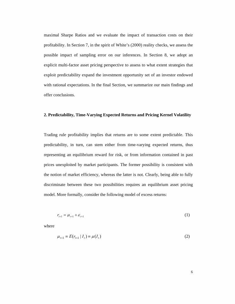
model. More formally, consider the following model of excess returns:

111 +++ += tttr εµ (1)

where

)()|( 11 tttt IIrE µµ ≡≡ ++ (2)

7

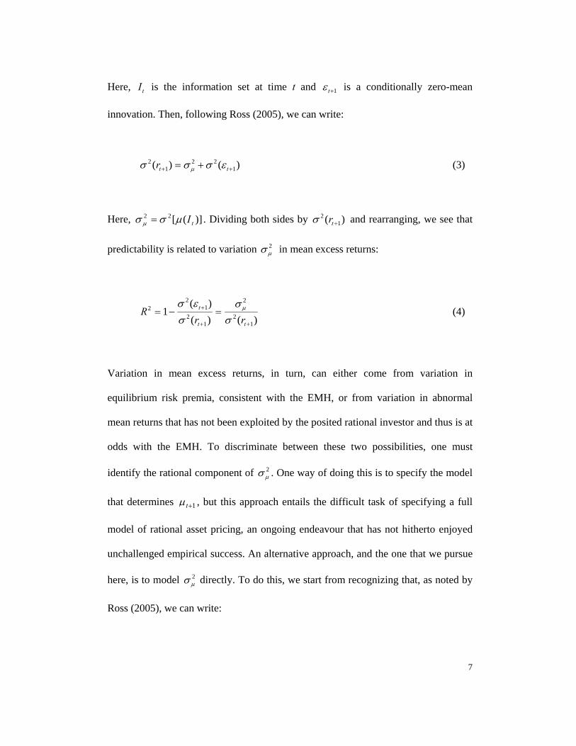
Here, tI is the information set at time t and 1+tε is a conditionally zero-mean

innovation. Then, following Ross (2005), we can write:

)()( 122

12

++ += ttr εσσσ µ (3)

Here, )]([22tIµσσ µ = . Dividing both sides by )( 1

2+trσ and rearranging, we see that

predictability is related to variation 2µσ in mean excess returns:

)()(

)(1

12

2

12

12

2

++

+ =−=tt

t

rrR

σσ

σεσ µ (4)

Variation in mean excess returns, in turn, can either come from variation in

equilibrium risk premia, consistent with the EMH, or from variation in abnormal

mean returns that has not been exploited by the posited rational investor and thus is at

odds with the EMH. To discriminate between these two possibilities, one must

identify the rational component of 2µσ . One way of doing this is to specify the model

that determines 1+tµ , but this approach entails the difficult task of specifying a full

model of rational asset pricing, an ongoing endeavour that has not hitherto enjoyed

unchallenged empirical success. An alternative approach, and the one that we pursue

here, is to model 2µσ directly. To do this, we start from recognizing that, as noted by

Ross (2005), we can write:

8

)()()1()( 12

1222

12

+++ +≤≤ ttft mrRE σσµσ µ (5)

Here, fR denotes the unconditional risk-free rate. The first inequality in (5),

)()]([ 21

211

2+++ ≤−= ttt EEE µµµσ µ , is based on an elementary result from

descriptive statistics. The second inequality follows from the fact that, under no-

arbitrage and in a friction-less economy, the pricing kernel satisfies

)|,()1( 111 tttft ImrCovR +++ +=µ , while the correlation between the kernel and the

asset excess return is bounded from above, in absolute value, by one. Using (5) in

(4), we see that predictability is bounded from above by a quantity that depends on

the amount of volatility of the kernel that prices the assets:

)()1( 1222

++≤ tf mRR σ (6)

Notably, the restriction in (6) holds unconditionally and thus for the in-sample

coefficient of determination of any predictive regression. Under the rational

expectations (RE) assumption originally formulated by Muth (1961), there is a tight

link between the pricing kernel 1+tm and investors’ marginal utility. The RE

assumption, in turn, is a necessary condition for the EMH to hold. These

considerations suggest one way to mitigate the stark alternative between having to

conduct a joint test of market efficiency and of a particular asset pricing model and

not being able to discriminate between time-variation in equilibrium returns and

abnormal profitability. A possible solution is to impose just enough restrictions on

9

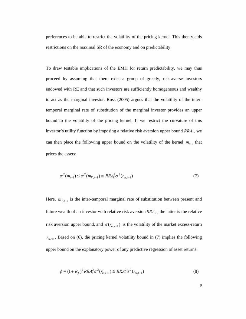
preferences to be able to restrict the volatility of the pricing kernel. This then yields

restrictions on the maximal SR of the economy and on predictability.

To draw testable implications of the EMH for return predictability, we may thus

proceed by assuming that there exist a group of greedy, risk-averse investors

endowed with RE and that such investors are sufficiently homogeneous and wealthy

to act as the marginal investor. Ross (2005) argues that the volatility of the inter-

temporal marginal rate of substitution of the marginal investor provides an upper

bound to the volatility of the pricing kernel. If we restrict the curvature of this

investor’s utility function by imposing a relative risk aversion upper bound RRAV, we

can then place the following upper bound on the volatility of the kernel 1+tm that

prices the assets:

)()()( 1,22

1,2

12

+++ ≅≤ tmVtVt rRRAmm σσσ (7)

Here, 1, +tVm is the inter-temporal marginal rate of substitution between present and

future wealth of an investor with relative risk aversion VRRA , the latter is the relative

risk aversion upper bound, and )( 1, +tmrσ is the volatility of the market excess-return

1, +tmr . Based on (6), the pricing kernel volatility bound in (7) implies the following

upper bound on the explanatory power of any predictive regression of asset returns:

)()()1( 1,22

1,222

++ ≅+≡ tmVtmVf rRRArRRAR σσφ (8)

10

Thus, under the EMH, we should observe φ≤2R and hence )( 1,222

+≤ tmV rRRAR σ .

To fix ideas, we may define a ‘boundary violation index,’ henceforth BVI, as the

difference between the coefficient of determination of the estimated predictive

regression and the predictability bound, i.e. φ−= 2RBVI . The inequality in (6)

implies that BVI should be non-positive for all predictive regressions of the returns

on all traded assets priced by the kernel m.

To operationalize (8), we need to specify the RRA upper bound RRAV. Ross (2005)

suggests imposing an upper bound of 5 on the relative risk aversion of the marginal

investor, i.e. 5≤VRRA . Among the motivations advanced by Ross (2005) to do so,

the one that most easily applies to a world with possibly non-normally distributed

returns and non-quadratic utility is the simple observation that a relative risk aversion

higher than 5 implies that the marginal investor would be willing to pay more than 10

percent per annum to avoid a 20 percent volatility of his wealth (i.e., about the

unconditional volatility of the S&P from 1926) which, by introspection, seems large.

It might be questioned whether a risk aversion upper bound of 5 is large enough in

light of evidence, provided by the empirical literature on the “equity premium

puzzle,” that points to much larger values. For example, Mehra and Prescott’s (1985)

seminal study suggests that, given the real rate of return on risk free assets, risk

aversion in excess of 50 is needed to explain the US equity premium in a model with

frictionless capital markets and standard preference assumptions. As formally shown

11

by Ross (2005), however, requiring the upper bound on RRA to exceed such

empirical lower bounds provided by the literature on the “equity premium puzzle”

would neglect the important circumstance that it is the marginal investors' risk

aversion that matters, not the average investor's one, and in the former the risk

aversion of wealthier and less risk averse investors takes a much larger weight than in

the latter. Related arguments offered by Ross (2005) draw on the reasonable idea that

aggregate consumption is much less volatile than the portfolio realistically held by

the marginal investors, i.e. by investors who have the capacity of influencing prices.

A study by Meyer and Meyer (2005) has recently provided a comprehensive re-

evaluation of the hitherto rather scattered empirical evidence on investors’ risk

aversion. They show that relative risk aversion estimates reported by the extant

literature are less heterogeneous and extreme if one takes into account measurement

issues and the outcome variable with respect to which each study defines risk

aversion. Using returns on stock investments as the outcome variable, calculations by

Meyer and Meyer (2005) show that the RRA coefficient in the classical Friend and

Blume’s (1975) study of household asset allocation choices ranges between 6.4 and

2.0, and decreases in investors’ wealth. Using returns on the investors’ overall

wealth, including real estate and a measure of human capital, the RRA estimate

ranges between 3.0 and 2.4. The same calculations show that the RRA implied by

Barsky et al. (1997) experiment ranges between 0.8 and 1.6.1 Importantly, these

1 When Meyer and Meyer (2005) consider estimates provided by studies based on asset pricing data, e.g. studies of the equity premium puzzle, they calculate somewhat higher values. Since in these studies the estimates of risk aversion are backed out parametrically from estimates of a particular asset

12

estimates, at least for the wealthiest cohorts of investors, are always considerably

lower than 5, i.e. the upper bound suggested by Ross (2005).

In light of the evidence reviewed by Meyer and Meyer (2005), alongside the RRA

upper bound of 5 suggested by Ross (2005), we will also experiment with a lower

value for the RRA upper bound, i.e. 5.2=VRRA . This value is just above the relative

risk aversion of the marginal investor in the stock market, if we assume that this

investor’s preferences are described by a power utility function and we estimate the

mean and volatility of the stock market using the historical average and standard

deviation of the returns on the S&P index since 1926. This bound implies that the

marginal investor would be willing to pay up to 5 percent per annum, arguably still a

relatively large amount, to avoid a 20 percent volatility of his wealth.

3. Data

Our data comprise daily and monthly returns on the spot exchange rate against the

US Dollar of the major currencies (except those that were replaced by the Euro) for

the period 1971-2006 taken by Bloomberg at the close of business in London at 6:00

p.m. GMT.2 These currencies are the Australian and Canadian Dollar (AUD and

CAD, respectively), the Japanese Yen (JPY), the British Pound (GPB), the Swiss

pricing model, often based on a narrow definition of the market portfolio, they are of no interest for the purpose of computing the SDF volatility bound. Their use would imply a circular argument. 2 We also use daily data, provided by Bloomberg, on the front month futures contract on the exchange rate of each of the above currencies against the US Dollar traded on the Chicago Mercantile Exchange (CME), but the results are not reported because they are qualitatively indistinguishable from, and quantitatively very similar to, the results for the underlying currencies.

13

Franc (CHF) and the Euro (denoted as ECU/EUR because we combine data on the

ECU before the introduction of the Euro in 1999 and on the latter after its launch). To

proxy for the return on the market portfolio we use daily and monthly returns on the

S&P500 index constructed from last traded price and dividend data provided by

Datastream.

4. Currency Returns Predictability

To conduct our tests of currency market efficiency, we estimate simple predictive

regressions of the returns on the currencies in our sample. Next, we construct

empirical counterparts to the predictability bound in (8) and we compare the

coefficient of determination of the estimated predictive regressions with the

constructed bound. As shown by Taylor (1994), among others, ARIMA models of

exchange rates, and thus ARMA models of currency returns, capture substantial

predictability. Our estimated models are thus specifications of the general

ARMA(p,q) model, where p denotes the autoregressive lag order and q denotes the

order of the moving average term:

yt = const. + b1yt-1 + ..... + bpyt-p + c1ut-1 + ..... + cqut-q + ut (9)

We apply versions of (9) to both currency returns and to returns adjusted by the

interest differential (i.e. the differential between the funding cost in US Dollars and

14

the return from reinvesting the funds in each one of the foreign currencies).3 We find

that adjusting returns for the interest differential has virtually no impact on estimated

predictability. This is because the volatility of the interest differential is negligible

relative to currency returns volatility. Thus, to avoid duplication of indistinguishable

predictability estimates, in the remainder of this study we work with currency return

data only.

We start by estimating specifications of (9) over rolling windows of daily and

monthly data for all currency returns in our sample, and recording their coefficients

of determination. The predictive models are ARMA(5,0) or, equivalently, AR(5), for

daily returns, and ARMA(5,2) for monthly returns. These specifications are chosen

because they capture reasonably well the predictability of currencies in our sample,

as suggested by Ljung-Box (1978) tests of the null of residual serial correlation,

rejected for lags of up to the 36th order.4 The estimation window l is one year, i.e. l =

252 trading days, for daily data and 5 years, i.e. 60125 =×=l months, for monthly

data. In other word, each predictive autoregression is estimated over a window that

runs between t-l and t, where window length l equals 252 for daily data and 60 for

monthly data. For each currency i, this yields daily and monthly series of coefficients

3 As a proxy for the risk-free rate on assets denominated in the currencies included in our dataset, we use daily middle rate data on Australian Dollar and German Mark inter-bank ‘call money’ deposits, on Canadian Dollar and Swiss Franc Euro-market short-term deposits (provided by the Financial Times/ICAP), on inter-bank overnight deposits in GBP and the middle rate implied by Japan’s Gensaki T-Bill overnight contracts (a sort of repo contract used by arbitrageurs in Japan to finance forward positions). The rate on German Mark deposits is used as a proxy for the rate at which it is possible to invest funds denominated in ECU, while the overnight Euribor is used as a proxy for the rate at which it is possible to invest Euro denominated funds. As a proxy for the US risk-free rate, we use daily data on 1 month T-Bills (yields implied by the mid-price at the close of the secondary market). The interest rate data are taken from Datastream. 4 The results of these tests are not tabulated to save space, but they are available from the authors upon request.

15

of determination 2)(, tltiR →− estimated over rolling estimation window of returns from

t–l to t. To estimate a time-varying predictability bound tφ at the daily (monthly)

frequency, we proxy for the variance of the market return between t-l and t, i.e.

)( ,&2

)( sltPStlt r +−→−σ with ]..... 2 ,1[ ls∈ , as the average, over rolling windows of 1 year

(5 years) of daily (monthly) GARCH(1,1) S&P500 returns sltPSr +−,& . To compute

tφ , as prescribed by (7), we then multiply )( ,&2

)( sltPStlt r +−→−σ by the square of the

chosen RRA upper bound, i.e. by the square of the chosen value of RRAV.

The resulting daily time-series of the rolling coefficients of determination for each

currency are plotted in Figure 1, against the time series of the rolling predictability

bound tφ computed by setting RRAV = 5. The corresponding monthly series are

qualitatively similar and they are not shown to save space.5 Visual inspection of

Figure 1 reveals that the coefficients of determination of the estimated

autoregressions are almost always above the bound. In fact, perhaps surprisingly,

sub-periods when the bound is not violated represent the exception rather than the

norm. As a consequence, as detailed in Table 1, the BVI is positive in more than 90

percent of the yearly rolling estimation windows for all currencies over the period

1971-2006 and three sub-periods of roughly equal length 1971-1983, 1984-1995,

1996-2006. Perhaps more remarkably, for most currencies and sub-periods, the

frequency of positive BVI values, and thus predictability upper bound violations, is

almost 100 percent.

5 They are however available from the authors upon request.

16

5. Economic Significance of Predictability

There is a tight link between predictability and the Sharpe ratio (SR) of strategies

designed to exploit it. This link can be used to express predictability in units that

have an immediate economic interpretation. To begin, it is worth recalling that, by a

familiar Hansen and Jagannathan (1991) result, the economy maximal Sharpe ratio,

and thus the maximum amount of profitability per unit of risk from any trading

strategy is bounded from above by the volatility of the pricing kernel:

)()1()()(

11

1+

+

+ +≤= tft

t mRSRr

Eσ

σµ

(10)

Thus, from (6) and (10), it is clear that the volatility of the pricing kernel places an

upper bound on both predictability and the maximal SR of the economy. This

circumstance can be seen as a consequence of the fact that the coefficient of

determination of predictive regressions can itself be interpreted as a maximal Sharpe

ratio. To show this, we use an elementary statistical result that relates the variance of

a random variable to its second moment and the square of its mean, and re-write the

coefficient of determination in (4) as follows:

( ) 2

21

2

212

22

22 11

rrrr

DDTDD

TTR

σµµµ

σµµµµµµ

σσ

σ µ −′′=−⎟⎠⎞

⎜⎝⎛ ′′=⎟

⎠⎞

⎜⎝⎛ −

′== −

−

(11)

17

Here, µ is the 1×T vector that stacks the conditional means of the currency return

at each point in time t, t = 1, ....T, µ is the unconditional mean return (a scalar) and

D denotes a TT × diagonal matrix with elements along the main diagonal that

contain the conditional standard deviation of the currency return at each point in time

t. In using this notation, we are essentially interpreting a strategy aimed at exploiting

predictability as a portfolio made up of as many positions as data points in the sample

period, each with its own ‘conditional’ SR. In monthly and higher frequency data, the

second term on the far right-hand side of (11) is negligible, as it is the square of a

typically small percentage number.6 In light of this, we can approximate the

coefficient of determination as follows,

( ) µµ 12 −′′≅ DDR (12)

Interestingly, if one neglects the possible temporal interdependencies across

conditional volatilities, i.e. if one neglects GARCH effects, (12) implies that the

coefficient of determination in predictive regressions can be interpreted as the

squared maximal SR attainable by forming ‘portfolios,’ i.e. strategies, of one-period

positions in the currency under consideration. Up to a constant of proportionality, the

weights with which each one-period position enters such strategy are then

( ) µ1−′= DDW (13)

6 Currencies have typically a drift rate very close to zero.

18

Intuitively, a trading strategy based on the above inter-temporal weights amounts to

using a predictive model that combines a directional signal, the conditional mean tµ ,

with a volatility filter, i.e. the elements tσ of D. These results are useful in that they

offer insights into the economic significance of predictability and help appreciate its

magnitude. Following this logic, we create an excess-predictability measure and,

based on (12), we express it in annualized Sharpe ratios units. To do so, we rely on

our boundary violation index introduced earlier ( φ−= 2RBVI ) and compute the

square root of its annualized value,

yearslBVI ttitti 1010 ,, →→ ≡γ

Here, 0t and 1t are the beginning and end points, respectively, of the sub-periods

over which we estimate 10, ttiBVI → and compute

10, tti →γ , i.e. 1971-1976, 1977-1982,

1983-1988, 1989-1994, 1995-2000 and 2001-2006. Clearly, 10, tti →γ is defined only

when 010, ≥→ttiBVI . The quantity under the square root is multiplied by the ratio of

the number of observations to the number of years in the estimation window length,

i.e. years

l , to annualize (thus, 252=years

l when working with 1-year estimation

windows of daily data and 12560

==years

l when using 5-year windows of monthly

data). The quantity 10, tti →γ has an appealing economic interpretation. Based on (12),

19

it can be seen as the annualized excess-SR that can be earned by exploiting

predictability, assuming that one trades at the indicated frequency (i.e. daily or

monthly). The value taken by 10, tti →γ , therefore, can be seen as a measure of “good

deal” availability.7

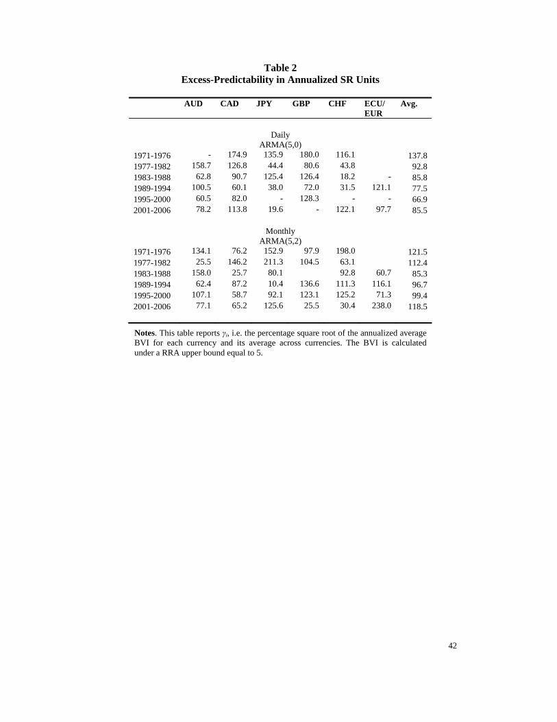
In Table 2, we report the computed values of 10, tti →γ based on estimates obtained

using daily and monthly data.8 These excess predictability measures are in many

cases positive and economically sizable. Excess-predictability is especially high in

the initial part of the sample periods, i.e. in 1971-1976. In subsequent periods, the

computed values of 10, tti →γ are generally lower, but a clear declining pattern can be

detected only in the values taken by the 10, tti →γ of AUD, except for a surge in the

final period, and to a lesser extent JPY. Except again for a surge in the final 5-year

period, such a declining trend is more evident, especially in the daily case, in the

arithmetic average of 10, tti →γ across all currencies reported in the last column. In the

case of ECU/EUR, there is a burst of predictability between 1989 and 1994, possibly

in relation to market adjustments leading to the adoption of the Euro.

Olson (2004) applies double moving-average rules to GBP, CHF, JPY and the

German Mark exchange rate against the US dollar and finds evidence that they would

7 We acknowledge that the empirical results are in-sample and may appear less convincing as evidence of “good deals” availability and thus EMH violations. However, our methodology is consistent with the essence of equation (6) and not a limitation. In addition, many currency speculators employed technical rules similar to (9) and captured returns in line with our calculations. 8 Again, the values of this quantity computed using monthly data are qualitatively similar and they are not tabulated to save space. They are however available upon request.

20

have generated abnormal profitability over the periods 1976-1980 and 1986-1990 but

also that excess-profitability disappeared after 1991. Neely, Weller and Ulrich (2007)

examine a more comprehensive set of trading rules and report similar findings. Large

values of our measure of excess-predictability 10, tti →γ , over the periods 1971-1976,

1977-1982 and, to a lesser extent, 1983-1988, are consistent with Olson’s (2004) and

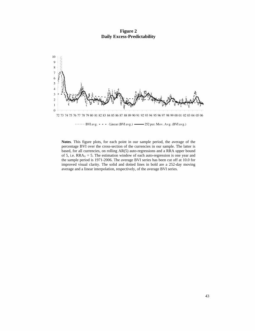
Neely, Weller and Ulrich’s (2007) findings. As shown in Figure 2, the average BVI

across our currencies declines over time and this is also broadly consistent with

evidence of diminishing abnormal profitability of technical trading rules reported by

these authors, in that decreasing excess-predictability presumably makes it more

difficult for technical trading rules to spot profitable trends.

Our findings, however, do not support the view that excess-predictability has

disappeared from the early 1990s onwards, or at least that it has been steadily

declining since then. To the contrary, the increase of the excess-predictability of a

number of currencies, in the latter part of the sample period, is in contrast with this

conclusion. To reconcile our evidence with the findings of diminishing profitability

of technical trading rules reported by Olson (2004) and Neely, Weller and Ulrich

(2007), one must posit that the rules considered by these authors do not capture all

predictability. Evidence provided by Pukthuanthong, Levich and Thomas (2007)

suggests that trend-following rules that were once profitable now lose money,

whereas the corresponding counter-trending rules, i.e. rules that do exactly the

opposite, are increasingly profitable. Our excess-predictability measure would

capture the excess-profitability of both types of strategies. Our results, contrary to

21

Olson’s (2004) and Neely, Weller and Ulrich’s (2007) findings, are also consistent

with evidence of high trading profits from momentum strategies during the 1990s

reported by Okunev and White (2003), as we generally do not find evidence of

declining excess-predictability after 1991.

On balance, our findings represent intriguing prima facie evidence that there is non-

negligible excess-predictability in currency markets and that this excess-

predictability, in recent years, has declined from its 1970s peaks without

disappearing entirely. This implies that there might be good reasons why currency

traders, in their pursuit of profitability and against academic advice, have long

engaged in technical analysis and other practices aimed at exploiting predictable

patterns in currency returns. Taken at face value, these results represent potential

evidence against the EMH. There is the possibility, however, that high transaction

costs might have to be incurred to exploit the estimated predictability and that our

estimates of the coefficient of determination R2 be inflated by sampling error. We

now investigate these important possibilities in turn.

6. The Impact of Transaction Costs

To gain insights into the impact of transaction costs, it is necessary to consider the

strategies that would have to be implemented in order to exploit the estimated

predictability. To this end, we use the weights in (13) to construct maximal SR

strategies for each currency and calculate their returns after transaction costs. Much

22

of the extant literature considers transaction costs of about 0.05 percent, or 5 basis

points, realistic for a typical round trip trade between professional counterparts, see

Levich and Thomas (1993) and Neely, Weller and Dittmar (1997). This corresponds

to about 2-3 basis points on each one way, i.e. buy or sell, transaction. In calculating

the return to these strategies, therefore, we allow for transaction costs of up to 5 basis

points. For comparison, we also experiment with transaction costs of 25 basis points.

In the context of our ARMA(p,q), the mean vector in (13) equals the conditional

mean of (9), i.e. ttt uy −=µ , while DD ′ collapses to the currency return sample

variance times a TT × identity matrix, i.e. TTt Iy ×+ )( 12σ .

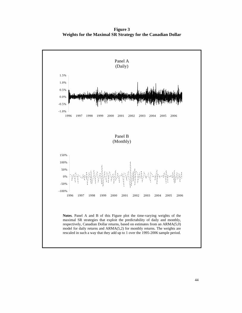
In Figure 3, to illustrate, we plot the time-varying weights, calculated using (13) and

normalized to add up to unity, of the maximal SR strategies that exploit the daily and

monthly predictability of the Canadian Dollar, based on AR(5) and ARMA(5,2)

specifications, respectively, estimated over the period 1995-2006. The corresponding

plots for other currencies, predictive models and sample periods are not reported to

save space. In all cases, there is substantial variation in the weights of the (daily)

positions entailed by the maximal SR strategies that optimally exploit daily

predictability, as a result of the conditional time-variation of the mean of the return

process. There is much less variation in the weights of the (monthly) positions

required to exploit monthly predictability. This means that strategies that exploit

daily predictability are rebalanced more frequently than those that exploit monthly

predictability and therefore transaction costs are likely to have a greater impact on

the former than on the latter. Notably, in classic filter and moving-average strategies,

23

trading positions change relatively infrequently.9 This is because such strategies often

exploit predictability at low frequency and thus avoid the burden of high transaction

costs.

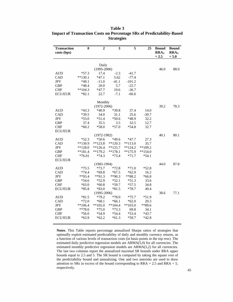
In Table 3, we report the SRs offered by maximal SR strategies that exploit daily and

monthly predictability. As before, the predictive model for daily returns is

ARMA(5,0) whereas the predictive model for monthly returns is ARMA(5,2). For all

the currencies under consideration, except CHF, transaction costs of 3 basis points

are enough to lower the SRs of the daily strategies below the level that corresponds

to the tightest predictability bound and the maximal SRs of the strategies based on

the daily predictability of AUD, JPY and ECU/Euro become negative. With

transaction costs of five basis points, the maximal SRs of daily strategies are negative

for all currencies. The strategies that exploit monthly predictability, however, are

much less sensitive to transaction costs. In all sub-sample periods, the SRs for the

maximal SR monthly strategies are positive even with transaction costs of 5 basis

points. More importantly, they often exceed the threshold implied by the

predictability bound, reported in the last two columns, even under RRAV = 5.

Crucially, this happens in the latter sample period too, contrary to studies cited earlier

which find that certain popular trading strategies are not profitable from the 1990s

onwards.

9 For example, Levich and Thomas (1993) report that over their 15 year sample period of major currencies, the 5 day / 20 day moving average rule traded 13 times per year.

24

Overall, these findings suggest that, while daily predictability cannot be exploited

because of high transaction costs, lower frequency (monthly) predictability might be

amenable to generate high SRs because trading frequency and transaction costs are

reduced. The latter circumstance poses a challenge to the EMH, as in an efficient

market investors endowed with rational expectations should detect excess-

predictability and recognize and exploit the attendant “good deal” opportunities,

thereby bringing predictability within the bound provided by the volatility of the

pricing kernel. In turn, this suggests that trading strategies based on low-frequency

currency predictability might be attractive for professional investors, at least for those

who can use available information better than the representative investor and face

moderate yet realistic levels of transaction costs.

A word of caution is in order at this point with respect to the likely magnitude of any

available “good deal.” There is substantial evidence that transaction costs depend on

the size of the transaction and, more specifically, on “price pressure.” For example,

Evans and Lyons (2002) estimate that a buy order of 1 million US dollars increases

the execution exchange rate against the Deutsche Mark and the Japanese Yen by as

much as 0.54 percent, or 54 basis points. Similar figures are provided by Berger,

Chernenko, Howorka and Write (2006), at least for trades executed over a daily

horizon. As shown in Table 3, transaction costs of 25 basis points are enough, with

few exceptions, to lower SRs below the threshold that corresponds to the wider

predictability bound, i.e. the bound corresponding to 5=VRRA , and often below the

level implied by the tighter predictability bound, i.e. the bound corresponding to

25

5.2=VRRA . Similar or higher levels of transaction costs, as implied by the evidence

provided by the literature on “price pressure,” are to be expected for large

transactions.

High transaction costs by themselves generate apparent excess-predictability. Roll

(1984), for example, show that the bid-ask bounce induces an amount of

predictability that depends on the relative magnitude of the bid-ask spread and

exchange rate variability. This predictability is not exploitable by construction,

because any attempt to exploit it would be costly. The evidence of high predictability

and these considerations on the impact of transaction costs on the profitability of

large-size transaction, taken together, allow one to rationalize, on the one hand, the

frequent occurrence of studies that find abnormally profitable strategies and, on the

other hand, the persistence of excess-profitability. We conjecture that available “good

deal” opportunities might persist over time because, though in principle

advantageous, they do not attract enough investors or investors with enough risk

capital, perhaps due to the presence of a fixed component of transaction costs, e.g.

entry costs. We leave, however, a formal investigation of this issue, i.e. the link

between transaction costs, transaction size and persistence of profit opportunities, for

future research.

26

7. The Impact of Sampling Error

To gain insight into the impact of sampling error on our assessment of excess-

predictability, we compare the estimated BVI with a measure of sampling error of the

coefficient of determination of the estimated predictive regressions. To this end, we

construct a modified version of the BVI, i.e. BVIadj, by reducing BVI by an amount

that reflects an estimate of sampling error at a specified confidence level,

%95,2.. Radj esBVIBVI −=

Here, %95,2.. Res denotes the sampling error, at the 95 percent confidence level, of the

estimated coefficient of determination of the predictive regression. To obtain an

estimate of sampling error, we use the asymptotic distribution of the coefficient of

determination 2R of the ARMA(p,q) model, valid when the model parameters are

estimated, derived by Hosking (1979), i.e.10

⎟⎟⎠

⎞⎜⎜⎝

⎛ − ∑∞

=1

222

22 )1(4 ,~ˆk

kTRRNR ρ

Here, 2R is the coefficient of determination under the null hypothesis and

)()(

t

kttk yE

yyE −=ρ denotes the k-th order autocorrelation of the series yt. In our case, yt

27

is a currency return and 2R is bounded from above by the predictability upper

bound, i.e. φ≤2R . The quantity ∑∞

=

−×

1

222 )1(464.1

kkT

R ρ , then, provides an

estimator of %95,2.. Res . Letting φ=2R , the above result can be rewritten to obtain a

convenient statistic for one-tailed tests that estimated predictability does not exceed

the upper bound φ , i.e.

⎟⎟⎠

⎞⎜⎜⎝

⎛−−= ∑

∞

=1

222 )1(4 ,0~)ˆ(k

kNRTH ρφφ

Because, as shown in Table 3 and discussed in the preceding section, the profitability

of strategies that exploit daily predictability is seriously affected by transaction costs,

we focus on the assessment of the statistical significance of monthly predictability.

The times series of BVIadj, based on ARMA(5,2) predictive regressions estimated

using rolling 5-year windows of monthly data, i.e. letting l = 60 and years = 5, are

plotted in Figure 4.11 The ARMA(5,2) predictive regressions are estimated using the

Broyden, Fletcher, Goldfarb and Shanno method described in Press et al. (1988). In

constructing BVIadj, we use ∑=

m

kkm 1

21 ρ as a sample counterpart of ∑∞

=1

21

kkT

ρ , where

15]2,4/min[ == llm .12 We do this because the computation of the variance of the

10 In the original article by Hosking (1979), the term (1 – R2) was not squared, but this error was subsequently amended by the author in an erratum. 11 The corresponding series constructed using daily data, i.e. using the coefficient of determination of ARMA(5,0) predictive regressions estimated over rolling 1-year windows of daily data, are qualitatively similar and are not plotted to save space. 12 We the implementation of this algorithm provided by the econometric software RATS™.

28

coefficient of determination, according to Hosking (1978), requires a consistent

estimate of ∑∞

=1

2

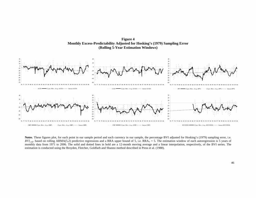
kkρ .13 Figure 4 shows that bursts of statistically significant excess-

predictability occurred at various points over the sample period, for example in the

1970s and 1980s, around the European Monetary System (EMS) crisis of the early

1990s and at the time of the Asian Financial Crisis in the second half of the 1990s. In

the more recent part of the sample period, the return on a number of currencies,

especially AUD, JPY, CHF and EUR also experienced episodes of significant

excess-predictability. Overall, as emphasized by the 12-month moving average

superimposed to the BVI series, statistically significant excess-predictability displays

a roughly cyclical pattern, i.e. periods of high and low predictability alternate over

time, consistent with Lo’s (2004) AMH. Suggestively, episodes of excess-

predictability appear to present themselves at times of changing economic conditions,

only to relatively quickly come to an end as market participants re-learn efficient

information processing, i.e. to do so in the context of the new economic conditions.

Next, we compute BVIadj over estimation windows corresponding to six 5-year long

non overlapping periods of roughly equal length between 1972 and 2006. We then

‘translate’ the computed BVIadj values into annualized SRs units, i.e. we construct a

version of 10, tti →γ adjusted for sampling error,

13 If we estimated the latter using m = ∞, we would have very few observations at our disposal to estimate autocorrelations of high orders, i.e. with k large and close to T. This would lead to inconsistent estimates of ρk and thus of the sampling error of R2.

29

years

lBVI ttiadjttiadj 1010 ,;,; →→ ≡γ

As before, 0t and 1t are the beginning and end points, respectively, of the sub-

periods over which we compute 10,; ttiadj →γ . We estimate BVIadj and

10,; ttiadj →γ using

both daily and monthly data but we tabulate results for monthly data only, due to the

high transaction costs that must be incurred to exploit daily predictability and thus

due to its likely limited economic significance. For the case of monthly data, the ratio

yearsl , that serves to annualize, equals 12. The quantity

10,; ttiadj →γ can be seen as the

annualized excess-SR that can be earned, at the 95 percent confidence level, by

exploiting excess predictability, assuming that one trades at the indicated frequency

(i.e., monthly). The predictive regressions, ARMA(5,2) for monthly data, are

estimated using maximum likelihood14. The constructed values of 10,; ttiadj →γ are

reported in Table 4, alongside Hosking’s (1978) H statistic and associated p-value of

the test that estimated predictability does not exceed the upper bound. They suggest,

in the 1980s, the presence of excess-predictability of AUD, JPY and, to a lesser

extent, CAD. The evidence of excess-predictability is still present in the 1990s for

GBP and CHF, with SRs in excess of the RRA = 5 bound as large as 9.67 and almost

38.81 percent, respectively. GBP also exhibits high statistically significant excess-

predictability in a number of periods.

14 We use the implementation of this method available in the econometric package RATS™.

30

The estimate of sampling error used to construct BVIadj might be biased or not

converge fast enough to provide a reliable estimate of sampling error of the

coefficient of determination of the estimated predictive regressions. In fact,

Hosking’s (1979) result is only valid asymptotically in large samples and it assumes

that the estimated predictive regression be the true data-generating model.15 This

might lead to an over-estimate of sampling error. To double-check on our assessment

of sampling error and especially as a further robustness check on our inferences

about the presence of excess-predictability, we bootstrap 2-tailed confidence intervals

for the coefficient of determination of the estimated predictive regressions. This

allows us to take sampling error of the coefficient of determination into account

without having to rely on large sample asymptotics and the normality assumptions

made by Hosking (1979). To conduct our bootstrapping experiment, we estimate the

parameters of the chosen predictive ARMA(p,q) model and store the residuals. We

then re-sample 1,000 times, with replacement, blocks of 5 consecutive realizations

from the stored residuals time-series, i.e. we employ ‘block re-sampling’ to capture

any residual serial correlation not explained by the estimated predictive regression.

Using the time-series of the re-sampled residuals and the point estimates of the

predictive regression parameters, we generate 1,000 separate bootstrapped currency

return series, for which we then re-estimate the chosen predictive ARMA(p,q) model

and record the coefficient of determination R2. This generates a bootstrapped

distribution of the latter. This approach to bootstrapping is known as estimation-

15 On a related note, Kurz-Kim and Loretan (2007) show that, in the case of the well-known finite sample F-distribution of the R2 under the null that the latter is zero, this might be a concrete danger when the normality assumption fails and the regression variables have fat tails distributions, as it is often the case for regressions involving currency returns.

31

based bootstrap. It has been introduced by Freedman and Peters (1984) and Peters

and Freedman (1984), and has been used by Karolyi and Kho (2004) to test the

profitability of momentum strategies.

In Table 5, we report monthly predictability upper bounds and bootstrapped

confidence intervals for the coefficient of determination of predictive regressions

estimated using monthly data. The predictive regressions are ARMA(5,2) and, for

comparison, more parsimonious ARMA(5,0). The predictive regressions are

estimated over the whole sample period and the three sub-periods 1971-1983, 1984-

1995, and 1996-2006. 16 When the predictive model is ARMA(5,0), evidence of

excess-predictability is not particularly strong. When one considers the explanatory

power of the ARMA(5,2) models, however, the bootstrapped confidence intervals are

almost always in excess of the tightest bound, i.e. the bound corresponding to RRAV

= 2.5. The wider bound, i.e. the bound corresponding to RRAV = 5.0, is violated in the

case of CAD and JPY in the initial 1971-1982 sub-sample period and in the case of

JPY also in the final sub-sample period, i.e. in 1995-2006.

To interpret these results, it is useful to consider that, when the 95th percentile of the

bootstrapped coefficient of determination distribution exceeds the predictability

bound for a given risk aversion bound RRAV, an investor endowed with rational

expectations and RRA no larger than RRAV could have exploited currency

predictability to reliably (i.e., with 95 percent confidence) generate SRs in excess of

the square root of the predictability bound. For example, by exploiting the monthly

32

ARMA(5,2) predictability of AUD, JPY and CHF over the period 1971-2006 and

under RRAV = 2.5, such an investor could have earned excess-SRs at least as large as

the square root of 1.28 percent. This amounts to an excess-SR of 39.2 percent per

annum. Similar calculations show that the same investor could have earned excess-

SRs of 40.1, 44.0 and 38.6 percent over the periods 1971-1983, 1984-1995, 1996-

2006, respectively, by exploiting the predictability of either currency in our sample

(except, of course, ECU/EUR over the initial sample period). The monthly

predictability of CAD and JPY over the period 1971-1983 and of JPY in 1996-2006

exceeds the predictability bound even under RRAV = 5.0. Thus, optimally exploiting

the monthly predictability of CAD and JPY over the period 1971-1983 and of JPY in

1996-2006 would have allowed for SRs in excess of 80.1 and 77.1 percent,

respectively.

The bootstrapped distributions of the coefficient of determination of predictive

regressions reported in Tables 5 provide stronger evidence of excess-predictability

than the estimates adjusted for Hosking’s (1979) sampling error reported in Table 4.

Both, however, suggest that an investor endowed with rational expectations could

have exploited predictability, over a number of portions of the 1971-2006 sample

period, to reliably generate SRs in excess of the good-deal thresholds corresponding

to RRAV = 2.5 or even RRAV = 5. Because the performance of strategies that exploit

monthly predictabilities is robust to transaction costs, this can be seen as evidence of

good-deal availability both before and after transaction costs. Such evidence becomes

weaker but does not entirely disappear in the more recent part of the sample period.

16 Tests for residual serial correlation are conducted using Ljung-Box (1978) Q-statistic.

33

This contrasts with the emerging view (in Taylor (2005) and Neely, Weller and

Ulrich (2007)) that the markets of the major currencies no longer allow for trading

profits.

8. Currency Predictability and the Investment Opportunity Set

To more explicitly assess to what extent predictability-based strategies expand the

investment opportunity set, we first combine the maximal SR strategies for the

individual currencies into an overall maximal SR strategy. We then compare the

performance of the latter to a benchmark currency management strategy, i.e. the AFX

index introduced by Lequeux and Acar (1998) and designed to track the performance

of technical analysis rules commonly followed by active currency managers.

Monthly values of this index are available from 1984 onwards. To take a

conservative stance on the amount of exploitable or detectable predictability, we

consider the maximal SR strategies that exploit the predictability implied by

parsimonious ARMA(5,0) models of monthly currency returns. We denote by r* the

excess return on the overall maximal SR strategy. The weights with which the

maximal SR strategies for the individual currencies enter the overall maximal SR

strategy, normalized to sum to one and reported in the first column of Table 6, are

calculated as follows:

*1** µ−

Σ=w (14)

34

Here, *Σ denotes the variance-covariance matrix of the returns on the individual

currencies maximal SR strategies and *µ denotes the vector of their unconditional

expected returns. As reported in the second column of Table 6, the SR of r* is

considerably higher than the SR of the individual currencies maximal SRs strategies.

Especially in the more recent sub-sample period, it is also much higher than the SR

of the AFX currency management index. In fact, while the SR of the AFX currency

management index is lower in 1996-2006 than in 1986-2006, the SR of r* is actually

much higher in the more recent sub-sample period. As shown in Table 7, the

correlation of the AFX index and r* drops from 52.36 percent in 1985-1990 to just

over 41 percent in 2003-2006. During the same time, while the SR of the AFX index

becomes negative, the SR of r* exceeds 106 percent per annum.

Taken together, these results suggest that the combination of moving-average rules

and currencies considered by the AFX index does not fully capture the estimated

amount of currency predictability, especially in recent times. Figure 5 shows the

rolling 12-month SR of the AFX index and r*. These series move remarkably closely

until about 1996 but subsequently their correlation breaks down. As shown in Table

7, their correlation becomes negative in 2003-2006. This suggests that, while the

excess-profitability of the specific moving average rules considered by the AFX

index might have dried up as market participants have employed them in their trading

strategies, alternative and not yet fully exploited sources of excess-profitability have

emerged and manifest themselves as excess-predictability. Again, this is consistent

35

with the Adaptive Market Hypothesis (AMH) perspective put forth by Lo (2004) and

advocated, in a currency market setting, by Neely, Weller and Ulrich (2007).

Finally, we take an explicit asset pricing perspective and we ask whether maximal SR

predictability-based strategies are spanned by known equity market factors, which

some studies suggest span the investment opportunity set. To this end, we simply

regress the excess return on each one of the individual currencies maximal SR

strategies, the overall SR strategy and, for comparison, the AFX currency

management index against the Fama and French (1993) factors, i.e. we estimate

titHMLitSMBitmmiiti HMLSMBrr ,,,,,, εβββα ++++= (15)

Here, tir , is the excess return on either the overall maximal SR strategy, rt*, an

individual currency maximal SR strategy or the AFX currency management index,

iα denotes the regression intercept, tmr , , SMBt and HMLt are the excess-returns on

the Fama and French (1993) market, size and book-to market factor mimicking

portfolios, respectively, and mi,β , SMBi,β and HMLi,β denote their corresponding

factor loadings, while ti,ε denotes the regression error term. As shown in Table 6, the

maximal SR strategies for a number of individual currencies and the overall maximal

SR strategy offer a positive and statistically significant αi, especially over the period

1984-2006. Perhaps more interestingly, the factor loadings on these strategies are

always either very small and statistically insignificant or negative and statistically

significant. This implies that the strategies either carry little systematic risk or they

36

act as a hedge against the latter.17 This fact, coupled with the sign and magnitude of

the factor loadings and the significance of the ‘alpha’ terms, suggest that the

strategies that exploit currency predictability expand the investment opportunity set,

i.e. they are not spanned by the Fama and French (1993) factors.

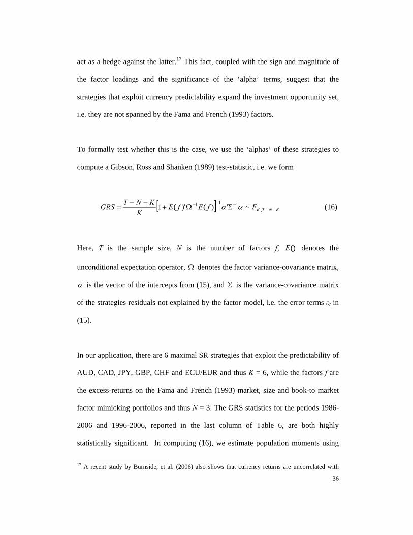
To formally test whether this is the case, we use the ‘alphas’ of these strategies to

compute a Gibson, Ross and Shanken (1989) test-statistic, i.e. we form

[ ] KNTKFfEfEK

KNTGRS −−−−− Σ′Ω′+

−−= ,

111 ~)()(1 αα (16)

Here, T is the sample size, N is the number of factors f, ()E denotes the

unconditional expectation operator, Ω denotes the factor variance-covariance matrix,

α is the vector of the intercepts from (15), and Σ is the variance-covariance matrix

of the strategies residuals not explained by the factor model, i.e. the error terms εt in

(15).

In our application, there are 6 maximal SR strategies that exploit the predictability of

AUD, CAD, JPY, GBP, CHF and ECU/EUR and thus K = 6, while the factors f are

the excess-returns on the Fama and French (1993) market, size and book-to market

factor mimicking portfolios and thus N = 3. The GRS statistics for the periods 1986-

2006 and 1996-2006, reported in the last column of Table 6, are both highly

statistically significant. In computing (16), we estimate population moments using

17 A recent study by Burnside, et al. (2006) also shows that currency returns are uncorrelated with

37

their sample counterparts. Gibson, Ross and Shanken (1989) demonstrate that

comparing the GRS statistic with the 5 percent critical value of its finite sample

distribution (under the null that pricing errors equal zero), i.e. the F distribution with

K and KNT −− degrees of freedom, amounts to testing whether the factors are on

the ex-post mean-variance frontier. The significance of the GRS statistic in our tests

thus implies that the Fama and French (1993) factors do not span the predictability-

based strategies and, therefore, that the latter expand the efficient frontier, at least

from the point of view of a rational mean-variance investor.

9. Conclusions, Final Remarks and Future Work

In this paper, we assess the statistical and, more importantly, economic significance

of predictability in currency returns over the period 1971-2006. We find that, even

under a relatively wide bound on relative risk aversion, predictability often violates

the attendant theoretically motivated upper bound. Closer scrutiny reveals that the

performance of strategies that attempt to optimally exploit daily predictability is very

sensitive to the level of transaction costs and this limits the extent to which it can be

exploited to generate genuine “good deals.” On the other hand, the performance of

strategies that attempt to optimally exploit monthly predictability is robust to

moderate yet realistic level of transaction costs. Taken at face value, this evidence

implies the availability of “good deals,” at least at the monthly frequency, and thus

violation of the EMH under a broad class of asset pricing models, for conservative

values of the marginal investor’s relative risk aversion and for realistic levels of

other asset classes.

38

transaction costs. Excess-predictability is highest in the 1970s and, for most

currencies in our sample, tends to decrease over time without disappearing. In

addition, we find that strategies based on monthly predictability expand the

investment opportunity set, even after transaction costs. This effect is also present in

the latter part of the sample period and, crucially, it does not disappear after the mid-

1990s, contrary to the conclusions of several recent studies. Taken together, our

findings pose a challenge to the EMH but they are consistent with Lo’s (2004)

AMH.18

Offering confirmation that technical trading is still alive in the currency domain,

Pojarliev and Levich (2008) have shown that currency hedge funds, behave as if they

follow standard technical trading strategies. Over the 1990-2006 period, the authors

show that a technical trading factor was the single most significant explanatory

variable of currency hedge fund returns. The returns of currency hedge funds were

significantly correlated with the AFX index over the 1990-2006 period. The

relationship declined somewhat over a 2001-06 sub-sample, but remained highly

significant. And in the present 2008 financial crisis, Deutsche Bank (2008) reports

that this year their technical trading currency benchmark has earned 8.8% over

LIBOR through October 20, similar to magnitudes observed in the 1970s and 1980s.

18 On a similar note, Lo (2005) offers, on pp. 35-36, a suggestive discussion of the cyclical behaviour of the first-order autocorrelation of the S&P Composite Index. In particular, on p. 35, Lo (2005) argues: “Rather than the inexorable trend to higher efficiency predicted by the EMH, the AMH implies considerably more complex market dynamics, with cycles as well as trends, and panics, manias, bubbles, crashes and other phenomena that are routinely witnessed in natural market ecologies. These dynamics provide the motivation for active management.”

39

A possible avenue of future research is a more formal investigation of whether the

estimated R2 series contains a time trend, a cyclical component and one or more

structural breaks. Considering cross-rates and a wider sample of countries, possibly

including emerging economies, might also allow the estimation of possible time

trends and structural breaks, perhaps adopting a panel approach. A random

coefficient model, along the lines of Swamy (1970), would appear particularly

promising to accommodate the difficulty of modelling possible sources of cross-

sectional variation in the predictability of currency returns. These extensions would

make it possible to better address the important question of whether predictability in

excess of a level that can be judged consistent with the EMH has become milder over

time as a result of learning by economic agents, or whether excess-predictability

exhibits a persistently cyclical pattern that can be more easily explained by Lo’s

(2004) AMH.

40

Figure 1 Daily AR(5) Predictability vs. Predictability Bound

Notes. These figures plot the sequences of the percentage coefficients of determinations (shown by the dotted line) of rolling AR(5) auto-regressions for each currency in our sample against their upper bound (shown by the solid line). The latter is computed under a relative risk aversion upper bound of 5. The estimation window of each auto-regression is one year and the sample period is 1971-2006. The values of all the series have been cut off at 2.0 to improve visual clarity.

0

0.5

1

1.5

2

2.5

1972 1975 1978 1981 1984 1987 1990 1993 1996 1999 2002 2005

AUD R Sq. Bound

0

0.5

1

1 .5

2

2 .5

1972 1975 1978 1981 1984 1987 1990 1993 1996 1999 2002 2005

CAD R Sq. Bound

0

0.5

1

1.5

2

2.5

1972 1975 1978 1981 1984 1987 1990 1993 1996 1999 200

JPY R Sq. Bound

0

0.5

1

1.5

2

2.5

1972 1975 1978 1981 1984 1987 1990 1993 1996 1999 2002 2005

GBP R Sq. Bound

0

0.5

1

1 .5

2

2 .5

1972 1975 1978 1981 1984 1987 1990 1993 1996 1999 2002 2005

CHF R Sq. Bound

0

0.5

1

1 .5

2

2 .5

1972 1975 1978 1981 1984 1987 1990 1993 1996 1999 200

ECU/EUR R Sq. Bound

41

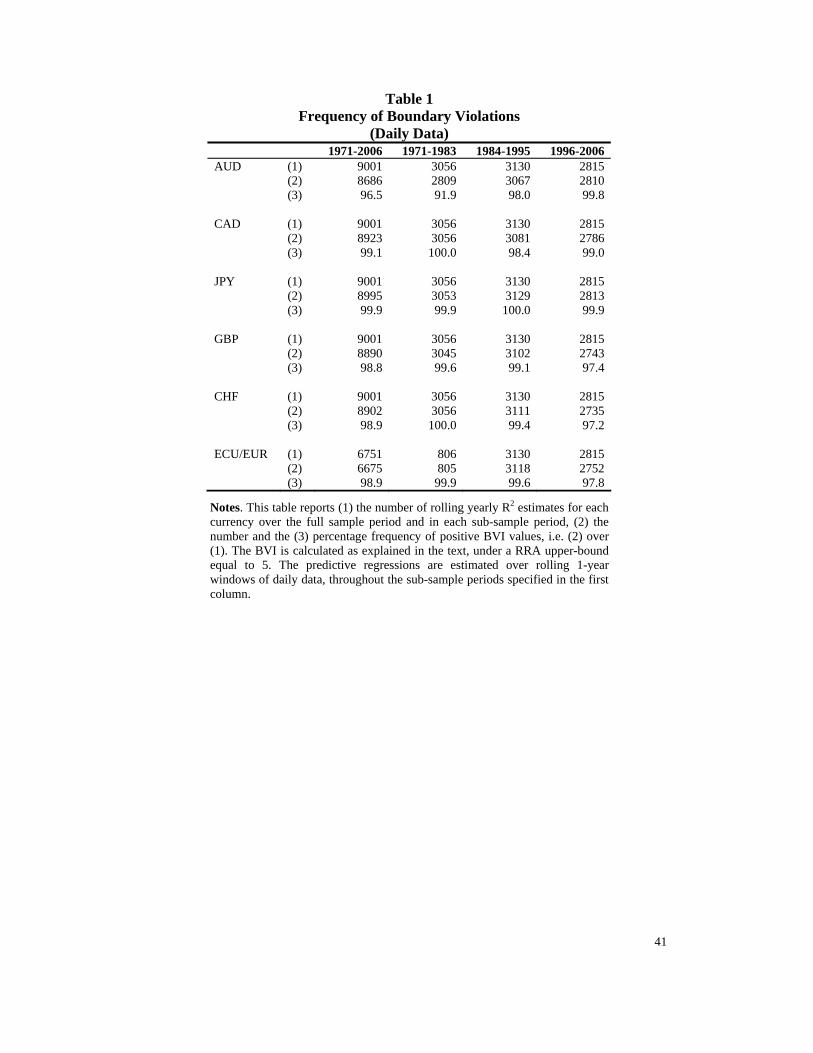
Table 1 Frequency of Boundary Violations

(Daily Data) 1971-2006 1971-1983 1984-1995 1996-2006 AUD (1) 9001 3056 3130 2815 (2) 8686 2809 3067 2810 (3) 96.5 91.9 98.0 99.8 CAD (1) 9001 3056 3130 2815 (2) 8923 3056 3081 2786 (3) 99.1 100.0 98.4 99.0 JPY (1) 9001 3056 3130 2815 (2) 8995 3053 3129 2813 (3) 99.9 99.9 100.0 99.9 GBP (1) 9001 3056 3130 2815 (2) 8890 3045 3102 2743 (3) 98.8 99.6 99.1 97.4 CHF (1) 9001 3056 3130 2815 (2) 8902 3056 3111 2735 (3) 98.9 100.0 99.4 97.2 ECU/EUR (1) 6751 806 3130 2815 (2) 6675 805 3118 2752 (3) 98.9 99.9 99.6 97.8

Notes. This table reports (1) the number of rolling yearly R2 estimates for each currency over the full sample period and in each sub-sample period, (2) the number and the (3) percentage frequency of positive BVI values, i.e. (2) over (1). The BVI is calculated as explained in the text, under a RRA upper-bound equal to 5. The predictive regressions are estimated over rolling 1-year windows of daily data, throughout the sub-sample periods specified in the first column.

42

Table 2 Excess-Predictability in Annualized SR Units

AUD CAD JPY GBP CHF ECU/

EUR Avg.

Daily

ARMA(5,0) 1971-1976 - 174.9 135.9 180.0 116.1 137.8 1977-1982 158.7 126.8 44.4 80.6 43.8 92.8 1983-1988 62.8 90.7 125.4 126.4 18.2 - 85.8 1989-1994 100.5 60.1 38.0 72.0 31.5 121.1 77.5 1995-2000 60.5 82.0 - 128.3 - - 66.9 2001-2006 78.2 113.8 19.6 - 122.1 97.7 85.5

Monthly

ARMA(5,2) 1971-1976 134.1 76.2 152.9 97.9 198.0 121.5 1977-1982 25.5 146.2 211.3 104.5 63.1 112.4 1983-1988 158.0 25.7 80.1 92.8 60.7 85.3 1989-1994 62.4 87.2 10.4 136.6 111.3 116.1 96.7 1995-2000 107.1 58.7 92.1 123.1 125.2 71.3 99.4 2001-2006 77.1 65.2 125.6 25.5 30.4 238.0 118.5

Notes. This table reports γi, i.e. the percentage square root of the annualized average BVI for each currency and its average across currencies. The BVI is calculated under a RRA upper bound equal to 5.

43

Figure 2 Daily Excess-Predictability

0

1

2

3

4

5

6

7

8

9

10

72 73 74 75 76 77 78 79 80 81 82 83 84 85 86 87 88 89 90 91 92 93 94 95 96 97 98 99 00 01 02 03 04 05 06

BVI avg. Linear (BVI avg.) 252 per. Mov. Avg. (BVI avg.)

Notes. This figure plots, for each point in our sample period, the average of the percentage BVI over the cross-section of the currencies in our sample. The latter is based, for all currencies, on rolling AR(5) auto-regressions and a RRA upper bound of 5, i.e. RRAV = 5. The estimation window of each auto-regression is one year and the sample period is 1971-2006. The average BVI series has been cut off at 10.0 for improved visual clarity. The solid and dotted lines in bold are a 252-day moving average and a linear interpolation, respectively, of the average BVI series.

44

Figure 3 Weights for the Maximal SR Strategy for the Canadian Dollar

Panel A (Daily)

Panel B (Monthly)

Notes. Panel A and B of this Figure plot the time-varying weights of the maximal SR strategies that exploit the predictability of daily and monthly, respectively, Canadian Dollar returns, based on estimates from an ARMA(5,0) model for daily returns and ARMA(5,2) for monthly returns. The weights are rescaled in such a way that they add up to 1 over the 1995-2006 sample period.

-100%

-50%

0%

50%

100%

150%

1996 1997 1998 1999 2000 2001 2002 2003 2004 2005 2006

-1.0%

-0.5%

0.0%

0.5%

1.0%

1.5%

1996 1997 1998 1999 2000 2001 2002 2003 2004 2005 2006

45

Table 3 Impact of Transaction Costs on Percentage SRs of Predictability-Based

Strategies

Transaction costs (bps)

0 2 3 5 25 Bound RRAV = 2.5

Bound RRAV = 5.0

Daily

(1995-2006) 46.0 88.0 AUD *57.3 17.4 -2.3 -41.7 CAD **130.1 *47.1 5.62 -77.4 JPY *49.1 -11.0 -41.1 -101.2 GBP *48.4 20.0 5.7 -22.7 CHF **104.3 *47.7 19.6 -36.7 ECU/EUR *82.1 22.7 -7.1 -66.6

Monthly

(1972-2006) 39.2 78.3 AUD *43.3 *40.9 *39.8 37.4 14.0 CAD *39.5 34.0 31.1 25.6 -30.7 JPY *53.0 *51.4 *50.6 *48.9 32.2 GBP 37.4 35.5 3.5 32.5 12.7 CHF *60.2 *58.0 *57.0 *54.8 32.7 ECU/EUR

(1972-1982) 40.1 80.1 AUD *52.3 *50.6 *49.6 *47.7 27.3 CAD **130.9 **123.8 **120.3 **113.0 35.7 JPY **128.0 **126.4 **125.7 **124.2 **109.2 GBP **181.4 **179.2 **178.1 **175.9 **154.0 CHF *76.01 *74.3 *73.4 *71.7 *54.1 ECU/EUR

(1983-1994) 44.0 87.8 AUD *75.5 *73.7 *72.8 *71.0 *52.8 CAD *74.4 *69.8 *67.5 *62.9 16.2 JPY **93.4 **91.3 **90.3 **88.2 *66.8 GBP *54.6 *52.9 *52.1 *51.3 33.6 CHF *63.0 *60.8 *59.7 *57.5 34.8 ECU/EUR *85.8 *83.0 *81.5 *78.7 49.4

(1995-2006) 38.6 77.1 AUD *81.5 *79.2 *78.0 *75.7 *51.9 CAD *72.0 *68.1 *66.1 *62.0 20.3 JPY **106.4 **105.0 **104.4 **103.0 **89.6 GBP **78.6 *75.0 *73.3 69.8 34.1 CHF *56.0 *54.9 *54.4 *53.4 *43.7 ECU/EUR *63.9 *62.2 *61.3 *59.7 *42.8

Notes. This Table reports percentage annualized Sharpe ratios of strategies that optimally exploit estimated predictability of daily and monthly currency returns, as a function of various levels of transaction costs (in basis points in the top row). The estimated daily predictive regression models are ARMA(5,0) for all currencies. The estimated monthly predictive regression models are ARMA(5,2) for all currencies. The last two columns report the annualized maximal SR bounds under RRA upper bounds equal to 2.5 and 5. The SR bound is computed by taking the square root of the predictability bound and annualizing. One and two asterisks are used to draw attention to SRs in excess of the bound corresponding to RRA = 2.5 and RRA = 5, respectively.

46

Figure 4 Monthly Excess-Predictability Adjusted for Hosking’s (1979) Sampling Error

(Rolling 5-Year Estimation Windows)

Notes. These figures plot, for each point in our sample period and each currency in our sample, the percentage BVI adjusted for Hosking’s (1979) sampling error, i.e. BVIi,adj. based on rolling ARMA(5,2) predictive regressions and a RRA upper bound of 5, i.e. RRAV = 5. The estimation window of each autoregression is 5 years of monthly data from 1971 to 2006. The solid and dotted lines in bold are a 12-month moving average and a linear interpolation, respectively, of the BVI series. The estimation is conducted using the Broyden, Fletcher, Goldfarb and Shanno method described in Press et al. (1988).

-70

-60

-50

-40

-30

-20

-10

0

10

20

30

76 77 78 79 80 81 82 83 84 85 86 87 88 89 90 91 92 93 94 95 96 97 98 99 00 01 02 03 04 05 06

AUD 12 per. Mov. Avg. (AUD) Linear (AUD)

-80

-60

-40

-20

0

20

40

76 77 78 79 80 81 82 83 84 85 86 87 88 89 90 91 92 93 94 95 96 97 98 99 00 01 02 03 04 05 06

CAD 12 per. Mov. Avg. (CAD) Linear (CAD)

-60

-50

-40

-30

-20

-10

0

10

20

30

40

76 77 78 79 80 81 82 83 84 85 86 87 88 89 90 91 92 93 94 95 96 97 98 99 00 01 02 03 04 05 06

JPY 12 per. Mov. Avg. (JPY) 12 per. Mov. Avg. (JPY) Linear (JPY)

-80

-60

-40

-20

0

20

40

76 77 78 79 80 81 82 83 84 85 86 87 88 89 90 91 92 93 94 95 96 97 98 99 00 01 02 03 04 05 06

GBP 12 per. Mov. Avg. (GBP) 12 per. Mov. Avg. (GBP) Linear (GBP)

-60

-50

-40

-30

-20

-10

0

10

20

30

40

76 77 78 79 80 81 82 83 84 85 86 87 88 89 90 91 92 93 94 95 96 97 98 99 00 01 02 03 04 05 06

CHF 12 per. Mov. Avg. (CHF) Linear (CHF)

-60

-50

-40

-30

-20

-10

0

10

20

30

76 77 78 79 80 81 82 83 84 85 86 87 88 89 90 91 92 93 94 95 96 97 98 99 00 01 02 03 04 05 06

ECU/EUR 12 per. Mov. Avg. (ECU/EUR) Linear (ECU/EUR)

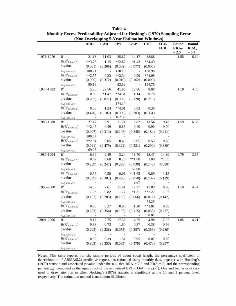
47

Table 4 Monthly Excess Predictability Adjusted for Hosking’s (1979) Sampling Error

(Non Overlapping 5-Year Estimation Windows) AUD CAD JPY GBP CHF ECU/

EUR Bound RRAV = 2.5

Bound RRAV = 5.0

1971-1976 R2 21.18 11.03 25.67 14.17 38.86 1.55 6.19 H(R2

RRA=2.5) **3.26 1.15 **2.82 *1.43 **4.49 p-value (0.001) (0.266) (0.002) (0.077) (0.000) γadj,RRA=2.5 108.21 - 110.19 - 168.98 H(R2

RRA=5.0) **2.55 0.33 **2.34 0.99 **4.08 p-value (0.005) (0.372) (0.010) (0.162) (0.000) γadj,RRA=5.0 80.16 - 83.52 - 154.76 1977-1982 R2 5.30 22.56 41.96 13.86 8.08 1.19 4.76 H(R2

RRA=2.5) 0.56 *1.47 **4.31 1.14 0.78 p-value (0.287) (0.071) (0.000) (0.128) (0.219) γadj,RRA=2.5 - - 174.10 - - H(R2

RRA=5.0) 0.08 1.24 **4.01 0.83 0.38 p-value (0.470) (0.107) (0.000) (0.203) (0.351) γadj,RRA=5.0 - - 162.39 - - 1983-1988 R2 27.17 6.91 11.71 5.82 13.54 9.43 1.59 6.36 H(R2

RRA=2.5) **2.45 0.49 0.85 0.40 0.90 0.70 p-value (0.007) (0.313) (0.198) (0.345) (0.184) (0.241) γadj,RRA=2.5 100.57 - - - - - H(R2

RRA=5.0) **2.04 0.05 0.46 -0.05 0.55 0.28 p-value (0.021) (0.479) (0.322) (0.521) (0.290) (0.389) γadj,RRA=5.0 69.95 - - - - - 1989-1994 R2 6.39 9.49 3.24 18.70 13.47 14.39 0.79 3.15 H(R2

RRA=2.5) 0.62 0.68 0.28 **1.88 1.08 *1.35 p-value (0.269) (0.247) (0.389) (0.030) (0.140) (0.088) γadj,RRA=2.5 - - - 52.00 - - H(R2

RRA=5.0) 0.36 0.50 0.01 **1.65 0.89 1.13 p-value (0.359) (0.307) (0.496) (0.050) (0.187) (0.129) γadj,RRA=5.0 - - - 9.67 - - 1995-2000 R2 14.30 7.61 11.81 17.37 17.80 8.98 1.19 4.74 H(R2

RRA=2.5) 1.03 0.82 1.27 *1.51 **2.27 1.07 p-value (0.152) (0.205) (0.103) (0.066) (0.012) (0.142) γadj,RRA=2.5 - - - - 74.25 - H(R2

RRA=5.0) 0.76 0.37 0.86 1.20 **1.81 0.59 p-value (0.223) (0.354) (0.195) (0.115) (0.035) (0.277) γadj,RRA=5.0 - - - - 38.81 - 2001-2006 R2 9.17 7.75 17.36 4.75 4.98 7.02 1.05 4.21 H(R2

RRA=2.5) 0.83 0.72 1.60 0.37 0.38 0.56 p-value (0.203) (0.236) (0.055) (0.357) (0.353) (0.289) γadj,RRA=2.5 - - - - - - H(R2

RRA=5.0) 0.52 0.39 1.31 0.05 0.07 0.26 p-value (0.303) (0.350) (0.095) (0.479) (0.470) (0.397) γadj,RRA=5.0 - - - - - -

Notes. This table reports, for six sample periods of about equal length, the percentage coefficient of determination of ARMA(5,2) predictive regressions estimated using monthly data, together with Hosking’s (1979) statistic and associated p-value under the null that RRA = 2.5 and RRA = 5, and the corresponding percent γadj, computed as the square root of the annualized BVI – 1.64 × s.e.(R2). One and two asterisks are used to draw attention to when Hosking’s (1979) statistic is significant at the 10 and 5 percent level, respectively. The estimation method is maximum likelihood.

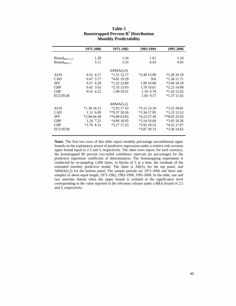
48

Table 5 Bootstrapped Percent R2 Distribution

Monthly Predictability

1971-2006 1971-1982 1983-1994 1995-2006 BoundRRA=2.5 1.28 1.34 1.61 1.24 BoundRRA=5 5.11 5.35 6.43 4.95

ARMA(5,0)

AUD 0.51 4.17 *1.51 12.17 *2.49 15.90 *1.28 10.18 CAD 0.47 3.77 *4.81 19.29 NA *1.36 11.71 JPY 0.57 4.28 *1.52 12.89 1.00 10.06 *3.96 18.18 GBP 0.42 3.63 *2.55 15.03 1.29 10.61 *2.23 14.08 CHF 0.52 4.22 1.09 10.51 1.18 9.78 *1.43 12.02 ECU/EUR 1.04 9.17 *1.37 11.62

ARMA(5,2)

AUD *1.38 24.15 *2.93 17.43 *5.15 23.39 *3.55 28.81 CAD 1.12 6.09 **9.37 30.36 *3.34 17.95 *3.33 15.52 JPY *2.94 64.38 **6.89 63.83 *4.23 27.30 **8.05 25.03 GBP 1.24 7.21 *4.80 18.05 *3.14 16.04 *3.93 18.26 CHF *1.76 8.31 *3.17 17.25 *3.92 19.55 *4.25 17.07 ECU/EUR *3.87 20.13 *3.36 14.62

Notes. The first two rows of this table report monthly percentage unconditional upper bounds on the explanatory power of predictive regressions under a relative risk aversion upper bound equal to 2.5 and 5, respectively. The other rows report, for each currency, the bootstrapped 90 percent two-tailed confidence intervals (in percentage) for the predictive regression coefficient of determination. The bootstrapping experiment is conducted by re-sampling 1,000 times, in blocks of 5 at a time, the residuals of the estimated monthly predictive model. The latter is AR(5), for the top panel, and ARMA(5,2) for the bottom panel. The sample periods are 1971-2006 and three sub-samples of about equal length, 1971-1982, 1983-1994, 1995-2006. In the table, one and two asterisks denote when the upper bound is violated at the significance level corresponding to the value reported in the left-most column under a RRA bound of 2.5 and 5, respectively.

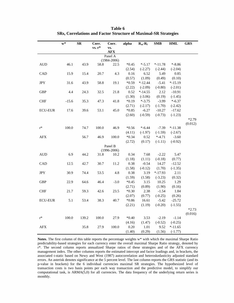
49

Table 6 SRs, Correlations and Factor Structure of Maximal-SR Strategies

w* SR Corr.

vs. r* Corr. vs. AFX

alpha Rm-Rf SMB HML GRS

Panel A (1984-2006)

AUD 46.1 43.9 58.8 22.5 *0.45 *-5.17 *-11.78 *-8.86 (2.54) (-2.27) (-2.44) (-2.04) CAD 15.9 15.4 20.7 4.3 0.16 6.52 5.49 0.85 (0.57) (1.09) (0.49) (0.10) JPY 31.6 43.9 58.8 19.1 *0.59 *-12.44 -5.41 *-15.19 (2.22) (-2.09) (-0.80) (-2.01) GBP 4.4 24.3 32.5 21.8 0.52 *-14.55 2.12 -10.91 (1.30) (-3.06) (0.19) (-1.45) CHF -15.6 35.3 47.3 41.8 *0.19 *-3.75 -3.99 *-6.37 (2.71) (-2.17) (-1.70) (-2.42) ECU-EUR 17.6 39.6 53.1 45.0 *0.85 -6.27 -10.27 -17.62 (2.60) (-0.59) (-0.73) (-1.23) *2.79

(0.012) r* 100.0 74.7 100.0 46.9 *0.56 *-6.44 -7.39 *-11.38 (4.11) (-1.97) (-1.59) (-2.67) AFX 56.7 46.9 100.0 *0.34 0.52 *-4.71 -3.60 (2.72) (0.17) (-1.11) (-0.92)

Panel B (1996-2006)

AUD 6.9 44.2 31.8 10.2 0.34 7.68 -2.22 5.47 (1.18) (1.11) (-0.18) (0.77) CAD 12.5 42.7 30.7 11.2 0.38 -0.54 14.27 -12.52 (1.58) (-0.12) (1.70) (-1.35) JPY 30.9 74.4 53.5 4.8 0.38 3.19 *-17.93 2.11 (1.59) (1.58) (-3.23) (0.32) GBP 22.9 64.6 46.4 -3.0 *0.45 3.15 10.25 1.29 (2.71) (0.89) (1.90) (0.16) CHF 21.7 59.3 42.6 23.5 *0.30 2.38 -1.54 1.84 (2.07) (0.77) (-0.25) (0.26) ECU-EUR 5.1 53.4 38.3 40.7 *0.86 16.61 -5.42 -25.72 (2.21) (1.19) (-0.20) (-1.55) *2.73

(0.016) r* 100.0 139.2 100.0 27.9 *0.40 3.53 -2.19 -1.14 (4.16) (1.47) (-0.52) (-0.25) AFX 35.8 27.9 100.0 0.20 1.01 9.52 *-11.65 (1.40) (0.29) (1.56) (-1.77)

Notes. The first column of this table reports the percentage weights w* with which the maximal Sharpe Ratio predictability-based strategies for each currency enter the overall maximal Sharpe Ratio strategy, denoted by r*. The second column reports annualized Sharpe ratios of these strategies and of the AFX currency management index. The other columns reports the estimated intercept and factor loadings and, in brackets, the associated t-static based on Newy and West (1987) autocorrelation and heteroskedasticity adjusted standard errors. An asterisk denotes significance at the 5 percent level. The last column reports the GRS statistic (and its p-value in brackets) for the 6 individual currencies maximal SR strategies. The hypothesized level of transaction costs is two basis points per each way transaction and the predictive model, to simplify our computational task, is ARMA(5,0) for all currencies. The data frequency of the underlying return series is monthly.

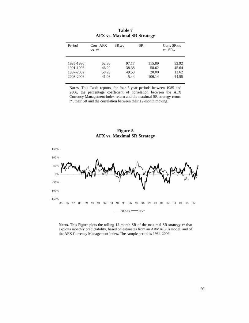
50

Table 7 AFX vs. Maximal SR Strategy

Period Corr. AFX

vs. r* SRAFX SRr* Corr. SRAFX

vs. SRr*

1985-1990 52.36 97.17 115.89 52.92 1991-1996 46.29 38.38 58.62 45.64 1997-2002 50.20 49.53 20.00 11.62 2003-2006 41.08 -5.44 106.14 -44.55

Figure 5 AFX vs. Maximal SR Strategy

-150%

-100%

-50%

0%

50%

100%

150%

85 86 87 88 89 90 91 92 93 94 95 96 97 98 99 00 01 02 03 04 05 06

SR AFX SR r*

Notes. This Figure plots the rolling 12-month SR of the maximal SR strategy r* that exploits monthly predictability, based on estimates from an ARMA(5,0) model, and of the AFX Currency Management Index. The sample period is 1984-2006.

Notes. This Table reports, for four 5-year periods between 1985 and 2006, the percentage coefficient of correlation between the AFX Currency Management index return and the maximal SR strategy return r*, their SR and the correlation between their 12-month moving.

51

Bibliography

Andersen, T.G., Bollerslev, T., Diebold, F.X. and H. Ebens, 2001, The Distribution of Stock Return Volatility, Journal of Financial Economics 61, 43-76. Andersen, T.G., Bollerslev, T., Diebold, F.X. and J. Wu, 2004, Realized Beta: Persistence and Predictability, PIER Working Paper No. 04-018. Barsky, R.B., F.T. Juster, M.S. Kimball, and M.D. Shapiro, 1997, Preference Parameters and Behavioral Heterogeneity: An Experimental Approach in the Health and Retirement Study, The Quarterly Journal of Economics 112, 537-539. Berger, D.W., Chaboud, A.P., Chernenko, S.V., Howorka E. and J.H. Write, 2006, Order Flow and Exchange Rate Dynamics in Electronic Brokerage System Data, Board of Governors of the Federal Reserve System. Box, G.E.P. and G.M. Jenkins (1976), Time Series Analysis, Forecasting and Control, San Francisco: Holden Day. Burnside, C., M. Eichenbaum, I. Kleschelski, and S. Rebelo. 2006. “The Returns to Currency Speculation,” NBER working paper 12916. Campbell, J.Y. and S.B. Thompson, 2005, Predicting the Equity Premium Out of Sample: Can Anything Beat the Historical Average? unpublished manuscript. Cerný, A. and S.D. Hodges, 2000, The Theory of Good-Deal Pricing in Financial Markets, Tanaka Business School Discussion Paper TBS/DP04/14. Cerný, A. and S.D. Hodges, 2001, The Theory of Good-Deal Pricing in Incomplete Markets, in Mathematical Finance-Bachelier Congress 2000, H. Geman, D. Madan, S. Pliska and T. Vorst, eds. Berlin: Spring, 175-202. Chang, P. H. K. and C.L. Osler, 1999, Methodical Madness: Technical Analysis and the Irrationality of Exchange-Rate Forecasts, The Economic Journal 109, 636-661. Cochrane, J.H., 2001, Asset Pricing, Princeton University Press, Princeton. Cochrane, J.H., 2005, Asset Pricing, 2nd Ed., Princeton University Press, Princeton. Cochrane, J.H. and J. Saà-Requejo, 2000, Beyond Arbitrage: Good Deal Asset Price Bounds in Incomplete Markets, Journal of Political Economy 108, 79-119. Deutsche Bank, 2008. “DB Currency Returns: Weekly Update,” October 20. Dooley, M.P. and J. Shafer. Analysis of Short Run Exchange Rate Behavior: March 1973 – September 1975, 1976, International Finance Discussion Papers, No. 76. Washington, D.C., Federal Reserve System.

52

Dooley, M.P. and J. Shafer, 1984, Analysis of Short-Run Exchange Rate Behaviour: March 1973–November 1981, in Bigman, D. and T. Taya (eds.), Exchange Rate and Trade Instability, Ballinger, Cambridge, MA. Evans, M.D.D., and R.K. Lyons, 2002, Order flow and exchange rate dynamics, Journal of Political Economy 110, 170–180. Fama, E., 1970, Efficient Capital Markets: a Review of Theory and Empirical Work, Journal of Finance 25, 383-417. Fama E. and K. French, 1993, Common Risk Factors in the Returns on Stocks and Bonds, Journal Financial Economics 33, 3-56. Freedman, D.A. and S.C. Peters, 1984, Bootstrapping an Econometric Model: Some Empirical Results, Journal of Business and Economic Statistics 2, 150-158. Friend, I. and M.E. Blume, 1975, The Demand For Risky Assets, American Economic Review 65, 900-922. Gelfand, A.E. and A.F.M. Smith, 1990, Sampling Based Approaches to Calculating Marginal Densities, JASA 85, 398-409. Gelman, A., Carlin, J.B., Stern, H.S. and Donald B. Rubin, 1995, Bayesian Data Analysis. London: Chapman and Hall. Gencay, R., 1999, Linear, Non-linear and Essential Foreign Exchange Rate Prediction with Simple Technical Trading Rules, Journal of International Economics 47, 91-107. Gibbson, M., Ross, S.A., and J. Shanken, 1989, A Test of The Efficiency of A Given Portfolio, Econometrica 57, 1121-1152. Hansen, L.P. and R. Jagannathan, 1991, Implications of Security Market Data for Models of Dynamic Economies, Journal of Political Economy 99, 225-262. Hosking, J.R.M., 1979, The Asymptotic Distribution of R2 for Autoregressive-Moving Average Time Series Models When Parameters Are Estimated, Biometrika 66, 156-7. Karolyi, G.A. and B.-C. Kho, 2004, Momentum Strategies: Some Bootstrap Tests, Journal of Empirical Finance 11, 509-536. Kurz-Kim, Jeong-Ryeol and M. Loretan, 2007, A Note on the Coefficient of Determination in Regression Models with Infinite-Variance Variables, Deutsche Bundesbank Discussion Paper, Series 1: Economic Studies, No 10/2007. LeBaron, B., 1999, Technical Trading Rule Profitability and Foreign Exchange Intervention, Journal of International Economics 49, 125-143.

53

Lequeux, P. and E. Acar, 1998, A Dynamic Index for Managed Currencies Funds Using CME Currency Contracts, European Journal of Finance 4, 311-330. Levich, R. M. and L.R. Thomas III, 1993, The Significance of Technical Trading-Rule Profits in the Foreign Exchange Market: A Bootstrap Approach, Journal of International Money and Finance 12, 451-74. Ljung, G.M. and G.E.P. Box (1978), On a Measure of Lack of Fit in Time Series Models, Biometrika 67, 297-303. Lo, A.W., 2004, The Adaptive Market Hypothesis: Market Efficiency from an Evolutionary Perspective, Journal of Portfolio Management, 30th Anniversary Issue, 15-29. Lo, A.W., 2005, Reconciling Efficient Markets with Behavioral Finance: The Adaptive Markets Hypothesis, Journal of Investment Consulting 7, 21-44. Mehra, R. and E. Prescott, 1985, The Equity Premium Puzzle, Journal of Monetary Economics 15, 145-161. Meyer, D.J. and J. Meyer, 2005, Relative Risk Aversion: What Do We Know? Journal of Risk and Uncertainty 31, 243-262. Neely, C., Weller, P., and R. Dittmar, 1997, Is Technical Analysis in the Foreign Exchange Market Profitable? A Genetic Programming Approach, Journal of Financial & Quantitative Analysis 32, 405-426. Neely, C.J., Weller, P.A. and J. Ulrich, 2007, The Adaptive Markets Hypothesis: Evidence from the Foreign Exchange Market, FRB of St. Louis Working Paper No. 2006-046B and forthcoming in the Journal of Financial & Quantitative Analysis. Available at SSRN: http://ssrn.com/abstract=922345 Nelson, C.R., 1972, The Interpretation of R2 in Autoregressive-Moving Average Time Series Models, The American Statistician 30, 175-180. Newy, W.K. and D.K. West, 1987, A Simple, Positive Semi-Definite, Heteroskedasticity and Autocorrelation Consistent Covariance Matrix, Econometrica 55, 703-8. Okunev, J. and D. White, 2003, Do Momentum-based Strategies Still Work in Foreign Currency Markets? Journal of Financial and Quantitative Analysis 38, 425-447. Olson, D., 2004, Have Trading Rule Profits in the Foreign Exchange Markets declined through time? Journal of Banking and Finance 28, 85-105.

54

Pesaran, M.H. and A. Timmermann, Predictability of Stock Returns: Robustness and Economic Significance, Journal of Finance 50, 1201-1228. Peters, S.C. and D.A. Freedman, 1984, Some Notes on the Bootstrap in Regression Problems, Journal of Business & Economic Statistics 2, 406-409. Pojarliev, M. and R.M. Levich. 2008. “Do Professional Currency Managers Beat the Benchmark?” Financial Analysts Journal, Sept/Oct.: 18-32. Press, W.H., Flannery, B.P., Teukolsky, S.A. and W.T. Vettering, 1988, Numerical Recipes in C, Cambridge University Press, New York. Pukthuanthong, K., Levich, R. M. and L.R. Thomas III, 2007, Do Foreign Exchange Markets Still Trend? Journal of Portfolio Management, vol. 34, no. 1 (Fall): 114-28.. Roll, R., 1984, A Simple Implicit Measure of the Effective Bid-Ask Spread in Financial Markets, Journal of Finance 39, 1127-1139. Ross, S.A., 1976, Arbitrage Theory of Capital Asset Pricing, Journal of Economic Theory 13, 341-60. Ross, S. A., 2005, Neoclassical Finance, Princeton University Press, Princeton, New Jersey. Schulmeister, S., 2006, The Interaction Between Technical Currency Trading and Exchange Rate Fluctuations, Finance Research Letters 3, 212-233. Stremme, A., Basu, D. and A. Abhyankar, 2005, The Optimal Use of Return Predictability: An Empirical Analysis, AFA 2006 Boston Meetings, paper available at SSRN: http://ssrn.com/abstract=687083. Swamy, P.A.V.B, 1970, Efficient Inference in a Random Coefficient Regression Model, Econometrica 38, 311-323. Sweeney, R. J., 1986, Beating the Foreign Exchange Market, Journal of Finance 41, 163-182. Taylor, S.J., 1994, Trading Futures Using a Channel Rule: A Study of the Predictive Power of Technical Analysis with Currency Examples, Journal of Futures Markets 14, 215-235. Taylor, S.J., 2005, Asset Price Dynamics, Volatility and Prediction, Princeton University Press, Princeton, NJ. White, H., 2000, A Reality Check for Data Snooping, Econometrica 68, 1097–1126.