Preventing Currency Crises in Emerging Markets

This PDF is a selection from a published volume from theNational Bureau of Economic Research

Volume Title: Preventing Currency Crises in Emerging Markets

Volume Author/Editor: Sebastian Edwards and Jeffrey A.Frankel, editors

Volume Publisher: University of Chicago Press

Volume ISBN: 0-226-18494-3

Volume URL: http://www.nber.org/books/edwa02-2

Conference Date: January 2001

Publication Date: January 2002

Title: What Hurts Emerging Markets Most? G3 ExchangeRate or Interest Rate Volatility?

Author: Carmen M. Reinhart, Vincent Raymond Reinhart

URL: http://www.nber.org/chapters/c10635

133

3.1 Introduction

Although fashions concerning appropriate exchange rate arrangementshave shifted over the years, advocacy for establishing a target zone sur-rounding the world’s three major currencies has remained a hardy peren-nial. Work on target zones (pioneered by McKinnon 1984, 1997, andWilliamson 1986, and recently summarized by Clarida 2000) has mostlyemphasized the benefits of exchange rate stability for industrial countries.More recently, though, analysts have apportioned some of the blame for fi-nancial crises in emerging markets back to the volatile bilateral exchangerates of industrial countries (as in the dissenting opinions registered inGoldstein 1999, for instance). With many emerging-market currencies tiedto the U.S. dollar either implicitly or explicitly, movement in the exchangevalues of the currencies of major countries—in particular the prolongedappreciation of the U.S. dollar in relation to the yen and the deutsche Markin advance of Asia’s troubles—is argued to have worsened the competitiveposition of many emerging market economies. One method for reducingdestabilizing shocks emanating from abroad, the argument runs, would beto reduce the variability of the Group of Three (G3) currencies by estab-

Carmen M. Reinhart, currently on leave from the University of Maryland, is senior policyadviser at the International Monetary Fund and a research associate of the National Bureauof Economic Research. Vincent Raymond Reinhart is director of the Division of MonetaryAffairs in the Board of Governors of the Federal Reserve System.

The authors have benefitted from helpful comments from Joshua Aizenman, Olivier Blan-chard, Guillermo Calvo, Michael P. Dooley, Eduardo Fernandez-Arias, Jeffrey A. Frankel,and Ernesto Talvi. Jane Cooley provided excellent research assistance. The views expressed arethe authors’ own and not necessarily those of their respective institutions.

3What Hurts Emerging Markets Most?G3 Exchange Rate or Interest Rate Volatility?

Carmen M. Reinhart and Vincent Raymond Reinhart

lishing target bands.1 This paper examines the argument for such a targetzone strictly from an emerging-market perspective and will be silent on thecosts and benefits for industrial countries.2

Given the reality that sterilized intervention by industrial economiestends to be ineffective and that policy makers show no inclination to returnto the kinds of controls on international capital flows that helped keep ex-change rates stable over the Bretton Woods era, a commitment to dampingG3 exchange rate fluctuations requires a willingness on the part of G3 au-thorities to use domestic monetary policy to that end. This, in turn, may re-quire tolerating more variability in interest rates and, potentially, spending.Under a system of target zones, then, relative prices for emerging-marketeconomies may become more stable in an environment of predictable G3exchange rates, but greater interest rate volatility may make debt-servicingcosts less predictable, and greater G3 income volatility may render demandsfor the products of emerging-market economies more uncertain. The wel-fare consequences to an emerging-market economy, therefore, are ambigu-ous, depending on initial conditions, the specification of behavior, and thedynamic nature of the trade-off between lower G3 exchange rate volatilityand higher G3 interest rate variability.

The consequences for the developing South of interest rate, exchangerate, and income volatility in the North comprise only one part of myriadNorth-South links. Consequently, issues related to G3 exchange rate vari-ability should be viewed within the much larger context (and related liter-ature) of the influence of economic outcomes in developed countries onthose in less developed economies. In this paper, we review and revisit the“traditional” North-South links via trade, commodity markets, and capitalflows, and add transmission channels in the form of interest rate and ex-change rate volatilities.

In section 3.2, we discuss the various channels of North-South transmis-sion and use the example of a simple trade model to establish that, for asmall open economy with outstanding debt, the welfare effect of dampingvariations in the exchange rate by making international interest rates morevolatile is ambiguous. Section 3.3 presents stylized evidence on how themonetary policy and economic cycle in the United States influence capitalflows to emerging markets as well as growth. In section 3.4, we first exam-ine the contribution of G3 exchange rate volatility to fluctuations in the ex-change rates of emerging markets and proceed to analyze the link between

134 Carmen M. Reinhart and Vincent Raymond Reinhart

1. Of course, since European monetary union, the G3 currencies cover at least fourteen in-dustrial countries—the United States, Japan, and the twelve nations that have adopted theeuro. In what follows, we splice together the pre–single currency data on the deutsche Markwith the post-1999 data on the exchange value of the euro.

2. For a cost-benefit analysis from a developed country’s perspective on the effects of limit-ing G3 exchange rate volatility or adopting a common currency, see Rogoff (2001). Of partic-ular relevance here is Rogoff’s argument that the strongest case for stabilizing major currencyexchange rates may well rest in the way that their volatility influences developing countries.

G3 interest rate and exchange rate volatility and capital flows and economicgrowth in developing countries. The final section summarizes our mainfindings and discusses some of the policy implications of our analysis.

3.2 North-South Links

In this section, we discuss the various channels through which economicdevelopments in the major developed economies can potentially affect de-veloping countries. On the developed side, we examine how the exchangerate arrangements among industrial countries influence the mix of interestrate and exchange rate volatility on world financial markets. On the emerg-ing markets side, our focus is on capital flows—their level and composi-tion—and on economic performance, as measured by gross domestic prod-uct (GDP) growth.

3.2.1 The Winds from the North: The Role of G3 Exchange Rate Arrangements in Determining the Mix of Interest Rate and Exchange Rate Volatilities

In principle, G3 exchange rates could be induced to stay within a targetband through some combination of three tools. First, national authoritiescould rely on sterilized intervention to enforce some corridor on bilateralexchange rates. However, except to the extent that such intervention tendsto signal future changes in domestic monetary policy, researchers havefound little empirical support that sterilized intervention in industrial coun-tries is effective.3 Second, national authorities could impose some form ofexchange or capital control, presumably in the form of a transactions tax orprudential reserve requirements. Opponents of such efforts generally arguethat capital controls generate financial innovation that undercuts them overtime, implying that the controls become either increasingly complicated orirrelevant. Third, monetary policy makers in the major countries could al-ter domestic market conditions to keep the foreign exchange value of theircurrencies in a desired range. This could take the form of allowing inter-vention in the currency market to affect domestic reserves—that is, not ster-ilizing intervention—or more directly keying the domestic policy interestrate to the exchange value of the currency (as discussed in McKinnon 1997and Williamson 1986).

Given the lack of evidence of any independent effect of sterilized inter-vention (over and beyond what subsequently happens to domestic mone-tary policy), and given the consensus supporting the free international mo-bility of capital, it would seem that the only instrument available to enforcea target zone would be the domestic monetary policy of the G3 central

What Hurts Emerging Markets Most? 135

3. The signaling channel is addressed by Kaminsky and Lewis (1996); Dominguez andFrankel (1993) examine whether there are any portfolio effects of sterilized intervention.

banks. However, this implies some trade-off, in that G3 domestic short-term interest rates would have to become more variable to make G3 ex-change rates smoother.

The nature of this trade-off, of course, depends on many factors, partic-ularly the width of the target zone. Wider bands would presumably reducethe need of G3 central banks to move their interest rates in response to ex-change rate changes. At the same time, however, wider bands would implya smaller reduction in the volatility of G3 exchange rates.4 In addition, G3interest rates might not be all that is affected by the exchange rate policy.Central bank actions taken to damp G3 exchange rate volatility might alsoleave their imprint on income in the G3 countries. Wider swings in indus-trial country interest rates would presumably make spending in those coun-tries more variable, even as the split of that spending on domestic versus for-eign goods and services becomes more predictable under more stable G3exchange rates.

To understand the effects of these trade-offs from an emerging-marketsperspective, it is important to remember that most developing countries arenet debtors to the industrial world and that typically that debt is short-termand denominated in one of the G3 currencies. As a result, the welfare con-sequences for an emerging-market economy of G3 target zones depend onexactly how those zones are enforced and the particulars of the small coun-try’s mix of output, trading partners, and debt structure.

3.2.2 A Stylized Model of an Emerging Market Economy

The effects of trading interest rate for exchange rate volatility can be seenin a basic single-period, two-good model of trade for a small open economy,as in figure 3.1. This figure represents a country that takes as given the rel-ative price of the two traded goods and receives an endowment in terms ofgood A. For the sake of simplicity, we assume that its external debt is alsodenominated in terms of good A and its currency is pegged to that of coun-try A.5 Volatility of the relative price of the traded goods—which mightstem solely from nominal changes in exchange rates between the industrialcountries if the small country fixes its exchange rate or if it prices to the in-dustrial country market—pivots the budget line and thus alters the desiredconsumption combination in the small country. Suppose, for instance, thatthe currency of country A depreciates relative to that of country B, rotating


4. Some might argue that if G3 target zones anchor inflation expectations in developedcountries, both exchange rates and interest rates could become more stable. However, many in-dustrial countries in the past decade have adopted some form of inflation targeting, either ex-plicitly or implicitly, which has worked to stabilize inflation expectations and which wouldmake achieving a credibility bonus from adopting a G3 target zone less likely.

5. Behind the scenes of this model in the larger industrial world, it is simplest to think of twolarge countries, A and B, specialized in the production of their namesake good. The net effectof our assumption about the small economy’s endowment and debt structure is that the inter-cept of the budget line depends on the interest rate in country A.

the budget line from EF to GF. All else being equal, welfare would decline,representing a cost associated with developments on the foreign exchangemarket for this small country.

Target zones for the large countries, if effective, would be able to preventthe budget line from rotating as the result of influences emanating from thedeveloped world. However, this reduced major-country exchange ratevolatility will only be accomplished if the major central banks change short-term interest rates in response to incipient changes in cross rates. For mostemerging-market economies, which are debtors, such coordination of G3monetary policy could deliver more stable terms of trade at the expense ofa more variable interest service. In this particular case, the central bank ofcountry A would presumably have to raise its domestic short-term interestrate in defense of the currency. Thus, while the slope of the budget linewould be unchanged, its location would shift inward, as labeled HI. Re-gardless of whether the effects of the initial shock were felt through the ex-change rate of the interest rate, welfare in this small country would decline.The degree to which it declines if the large countries allow the cross-exchange rate or their interest rates to adjust will depend on many factors.

3.2.3 Going Beyond the Stylized Model

In reality, many developing countries send primary commodities ontothe world market, there is some substitutability in world demand for thosecountries that produce manufactured products, and capital markets are farfrom perfect. In this section, we review the literature on North-South link-ages to broaden our understanding of the issues related to G3 exchange ratearrangements.

As opposed to the simple example, most emerging-market economies


Fig. 3.1 Welfare in a small open economy

face some slope to the demand curve for their exports. As a result, anychanges in G3 income induced by changes in their interest rates will be re-flected in the demand for the exports of their trading partners to the extentthat imports in the developed economy have a positive income elasticity.6

The higher the share of exports that are destined for the developed country,the more sizable the consequences for the emerging-market economy. Onthe basis of this channel, for example, Mexico and Canada would beaffected far more than Argentina by an economic downturn in the UnitedStates. We see evidence of this in the fact that in 1999 about 88 percent ofall Canadian and Mexican exports were shipped to the U.S. market,whereas only about 11 percent of Argentina’s exports were destined for theUnited States.7 Other things being equal, the higher the income elasticity ofimports in the developed country, the more pronounced will be the con-traction in the country’s exports when the developed country slows. In thisregard, developing countries that export predominantly manufacturedgoods (which typically are more sensitive to income) may fare worse thantheir counterparts exporting primary commodities, which tend to be rela-tively income-inelastic.8 The heterogeneity in export structure across devel-oping countries is sufficiently significant to expect, a priori, highly differen-tiated outcomes. For instance, the contrast between the export structure ofEast Asian countries (which are heavily skewed to manufactured goods) tothat of most African countries (which are predominantly skewed to pri-mary commodities) is particularly striking.9

As opposed to the simple example, emerging-market economies gener-ally produce a different mix of goods from those of industrial countries. Inthat case, the business cycle in the world’s largest economies may itself ex-ert a significant influence on the terms of trade of their smaller, developingtrading partners. Perhaps the clearest example of such a North-South linkcomes from international commodity markets, as argued in Dornbusch(1985). Beginning with that work, the literature on commodity price de-termination has consistently accorded a significant role to the growth per-formance of the major industrial countries.10 In particular, recessions inindustrial economies, especially the United States, have historically beenassociated with weakness in real commodity prices. In our simple example,


6. Note that this channel, as it relies on the behavior of the large partner, is present irre-spective of the level of development of the smaller trading partners.

7. The stylized evidence on patterns of trade is discussed in the next session.8. See, for example, Reinhart (1995), who estimates industrial countries’ import demand

function for various regions and countries with varying degrees of export diversification andprimary commodity content.

9. For example, manufactures account for only 10 percent in the Côte D’Ivoire (the IvoryCoast) but account for more than 65 percent of Thai exports.

10. Dornbusch (1985) stresses the role of the demand side in commodity price determina-tion. Borensztein and Reinhart (1994), who incorporate supply-side developments in theiranalysis, also find a significant and positive relationship between growth in the majoreconomies and world commodity prices.

if the small country’s endowment was made up of a commodity, the effectsof G3 monetary policy actions on overall demand for those primary goodscould induce a sizable shift in the position and rotation of the budget line.

Yet the impact of fluctuations in the business cycle on developingeconomies is probably not limited merely to income and relative priceeffects. There is a well-established, endogenous, and countercyclical “mon-etary policy cycle” in the major developed economies. To damp the ampli-tude of the business cycle, central banks ease monetary conditions and re-duce interest rates during economic downturns and hike interest rates whensigns of overheating develop. Calvo, Leiderman, and Reinhart (1993) stressthe importance of U.S. interest rates in driving the international capital flowcycle. They present evidence that, in periods of low interest rates in theUnited States, central banks in developing countries in Latin America sys-tematically accumulate foreign exchange reserves and the real exchangerate appreciates. Subsequent studies that examined net capital flows, ex-tending the analysis to a variety of their components over various sampleperiods and to developing countries in other regions, found similar evi-dence.

This link between the interest rate and capital flow cycle may arise for avariety of reasons. Investors in the developed economies faced with lowerinterest rates may be inclined to seek higher returns elsewhere (i.e., the de-mand for developing country assets increases). It also may be the case thatthe decline in international interest rates makes borrowing less costly foremerging markets and increases the supply of emerging-market debt. Inthat case, the decline in the cost of borrowing for emerging-market coun-tries may be even greater than the decline in international interest rates ifthe country risk premium is itself a positive function of international inter-est rates. The evidence presented in Fernandez-Arias (1996), Frankel,Schmukler, and Servén (2001), and Kaminsky and Schmukler (2001) sup-port the notion that country-risk premiums in many emerging markets in-deed move with international interest rates in a manner that amplifies theinterest rate cycle of industrial countries. Thus, a change in G3 interest ratesshifts the budget line by more than is shown in our simple example, as pro-cyclical capital flows imply that the change in the industrial country inter-est rate changes the developing country’s interest rate risk premium in thesame direction. Moreover, one could posit nonlinearities in the response iflarge increases in borrowing costs—from balance-sheet strains and creditrationing—have more substantial effects on income prospects than do sim-ilar size reductions in borrowing costs.

Table 3.1 provides a summary of the channels of transmission of howdevelopments in the major industrial countries may influence growth inemerging markets. Taken together, the various cells of the table would sug-gest that the trade and finance effects that arise in developed economiesfrom the growth and interest rate cycles, respectively, tend to at least par-


tially offset one another. However, G3 exchange rate and interest ratevolatility would seem a priori to have a negative effect on economic growthin the developing world. Higher interest rate volatility may hamper invest-ment, while higher G3 exchange rate volatility may retard emerging markettrade.11 While the literature on the impacts on trade of exchange rate volatil-ity for developed economies is inconclusive, the comparable analysis of thisissue for emerging markets seems much more convincing in concluding thatexchange rate volatility tends to reduce trade.


Table 3.1 Developed and Developing Country Links

Expected Growth Type of Shock Transmission Channel Amplifiers Consequences

The Growth Cycle: Recessions in the G3Income effects Trade: Lower exports to G3; High trade exposure; Negative

negative high G3 income elasti-cities

Relative price effects Trade: Decline in the terms High primary commo- Negativeof trade for developing dity content in exports; countries high exposure to cycli-

cal industries in exportsInternational capital Finance: Higher capital flows Large declines in the Positive

flows (primarily bank lending) to domestic demand for emerging markets bank loans

The Interest Rate Cycle: Monetary EasingsInternational capital Finance: Higher portfolio Developed bond and Positive

flows capital flows to emerging equity markets; high in-markets terest rate sensitivity

of flowsDebt servicing Finance: Lower cost High levels of debt; Positive

sensitive risk premiums to international interest rates

Interest earnings Finance: Declining interest High level of reserves Not obviousincome relative to debt

High Volatility in G3Interest rates Finance: Complicates debt High levels of short- Not obvious

management term debt; large new Investment: Uncertainty financing needs; antends to reduce investment initially high level of Negativeconsequences FDI

Bilateral exchange Trade: Reduces trade Pegging to a G3 Negative?rate currency

11. Of course, G3 interest rate volatility may also complicate significantly emerging marketdebt management strategies or make systemic strains more likely.

3.3 The Role of the North’s Business and Monetary Policy Cycles: The Stylized Facts

In this section, we present stylized evidence on the North-South linksthat were discussed in the preceding section. For emerging markets, we ex-amine international capital flows and growth around various measures ofthe U.S. growth and interest rate cycle and contrast periods of high inter-est rate and exchange rate volatility to those in which volatility was rela-tively subdued. We present evidence of the direction of North-South tradeand on the impact of G3 developments on international commodity mar-kets.

Our data are annual and span the years 1970 to 1999, and the countrygroupings are those reported in the International Monetary Fund’s WorldEconomic Outlook (WEO).12 For capital flows, these groupings include allemerging markets, Africa, Asia crisis countries, other Asian emerging mar-kets, the Middle East and Europe, and the Western Hemisphere. In report-ing aggregate real GDP, the WEO groups the Asian countries somewhatdifferently. The two reported subgroupings are Asia and newly industrial-ized Asia, but all other categories remain the same. We examine the cyclicalbehavior of net private capital flow and its components: net private directinvestment (i.e., foreign direct investment [FDI]), private portfolio invest-ment (PI), other net private capital flow (OCF)—which is heavily weightedtoward bank lending—and net official flow (OFF).

3.3.1 The Growth Cycle, Capital Flows, and Emerging Market Growth

Given its prominent position in the world economy, the U.S. businesscycle (not surprisingly) has important repercussions for the rest of theworld. Economic developments in the United States echo loudly in manydeveloped economies, most notably that of Canada; the same holds true fordeveloping economies, especially those in the Western Hemisphere andnewly industrialized Asia. To examine the behavior of growth and varioustypes of capital flows to emerging markets, we first split the sample into twostates of nature according to two criteria. The first parsing separates thesample into recessions and expansions according to the National Bureau ofEconomic Research’s dating of U.S. business cycle turning points. The sec-ond cut of the data divides the sample into periods in which U.S. real GDPgrowth is above the median growth rate for the sample and periods in whichgrowth is below the median.

Figure 3.2 depicts capital flows to emerging markets (in billions of 1970U.S. dollars) in recession years versus recovery years for the 1970–99 pe-riod. As is evident, net flows to emerging markets are considerably larger in


12. The developing country classification in the WEO is comprised of 128 countries. See theWEO for details on the regional breakdown.

Fig

. 3.2

U.S

. bus

ines

s cy

cle

and

capi

tal fl

ows

to e

mer

ging

mar

ket e

cono

mie

s (b

illio

ns o

f 197

0 U

.S. d

olla

rs):

A,N

et re

al p

riva

teca

pita

l flow

s; B

,Net

real

pri

vate

dir

ect i

nves

tmen

t; C

,Net

real

pri

vate

por

tfol

io in

vest

men

t; D

,Oth

er N

et re

al p

riva

te c

apita

l flow

sS

ourc

e:A

utho

rs’ c

alcu

lati

ons

usin

g In

tern

atio

nal M

onet

ary

Fun

d W

orld

Eco

nom

ic O

utlo

ok(O

ctob

er 2

000)

.

real terms when the United States is in expansion than when the UnitedStates is in recession. Furthermore, this gap between recession and expan-sion owes itself primarily to a surge in FDI flows (which increase almostthreefold from recession to expansion) and to portfolio flows (which in-crease almost fivefold from recession to expansion). The key offsetting cat-egory is other net inflows to emerging markets, which evaporate when theUnited States is in an expansion rather than recession. This disparate be-havior between FDI and portfolio flows is primarily due to bank lending,which accounts for a significant part of other flows. Apparently, banks tendto seek lending opportunities abroad when the domestic demand for loansweakens and interest rates fall, as usually occur during recessions. The U.S.bank lending boom to Latin America in the late 1970s and early 1980s andthe surge in Japanese bank lending to emerging Asia in the mid-1990s aretwo clear examples of this phenomenon.

However, the surge in FDI flows from the mid-1990s to the present is asignificant departure from FDI’s historical behavior, which is, no doubt,heavily influenced by the wave of privatization and mergers and acquisi-tions that took place in many emerging markets during recent years. It ispossible that because this period of privatizations and surging FDI coin-cides with the longest economic expansion in U.S. history, the results mayimply an exaggerated role for U.S. growth in driving FDI and total net flows.When we ended our sample in 1992, capital flows to emerging markets stilldiminished during economic downturns in the United States (this exerciseis not reproduced here). While FDI flows and portfolio flows continue to behigher in expansions than in recessions, the drop in other flows during ex-pansions more than offsets this tendency.

In sum, from the vantage point of the volume of capital flows to emerg-ing markets, U.S. recessions are not a bad thing. From a compositionalstandpoint, however, the more stable component of capital flows, FDI, doesseem to contract during downturns, suggesting that emerging markets maywind up during these periods relying more heavily on less stable sources offinancing—short-term flows.13

The analogous exercise was performed for emerging-market averageannual GDP growth. As shown in table 3.2, for all developing countries,growth is somewhat slower during U.S. recessions, averaging 4.8 percentper annum versus 5.2 percent average growth during expansion years. How-ever, the pattern is uneven across regions. For the countries in transition,Asia (including the newly industrialized economies), and the Middle Eastand Europe, growth tends to slow during U.S. recessions, while the oppo-site is true for Africa and the Western Hemisphere. However, in most in-stances the differences across regions are not markedly different—an issuewe will explore further later.


13. Other flows are mostly short term.

3.3.2 The Growth Cycle and Trade

If economic downturns in the United States are not necessarily bad forthe availability of international lending to emerging markets, slowdownsare likely to have adverse consequences for countries that rely heavily on ex-ports to the United States. Table 3.3 reports the percentage of total exports(as of 1999) of various emerging markets in Africa, Asia, and the WesternHemisphere that are destined for the U.S. market. It is evident that bilateraltrade links between the United States and the developing world arestrongest for Latin America, although there is considerable variation withinthe region, with Mexico and Argentina sitting at the opposite ends of thespectrum. However, trade between the United States and the Asian coun-tries shown in this table is by no means trivial, especially if one considersthat (as shown in table 3.4) the income elasticity in developed economies forAsian exports is typically estimated to be more than twice as large as the in-come elasticity for African exports; more generally, the income elasticity ofthe exports of developing countries that are major exporters of manufac-tured goods is well above that of those countries whose exports have ahigher primary commodity content.

As noted earlier, swings in the economic cycle in the United States andother major industrialized economies typically influence the terms of tradeof primary-commodity exporters. According to the various studies re-viewed in table 3.5, a 1 percentage point drop in industrial productiongrowth in the developed economies results in a drop in real commodityprices of roughly 0.77 to about 2.00 percent, depending on the study.

3.3.3 The Interest Rate–Monetary Policy cycle

In a world of countercyclical monetary policy in industrial countries, aneconomic cycle goes hand in hand with an interest rate cycle. As with the


Table 3.2 The Condition of the U.S. Economy and Foreign Real GDP Growth: Annual Rate (%) 1970–99

Condition of U.S.Monetary Policy:Condition of U.S. Economy:

Region/Country Expansion Recession Tightening Easing

Newly industrialized Asian economies 7.92 7.11 8.79 6.93

Developing countries 5.19 4.82 5.17 5.02Africa 2.75 3.29 2.63 3.10Asia 6.70 6.25 6.72 6.46Middle East and Europe 4.47 4.31 3.87 4.80Western Hemisphere 3.63 3.81 4.21 3.34

Source: Authors’ calculations using International Monetary Fund, World Economic Outlook (October2000).

Table 3.3 North-South Trade Patterns, 1999

Exports to the U.S. Imports from the U.S.Region/Country (% of Total Exports) (% of Total Imports)

Latin AmericaArgentina 11.3 19.6Brazil 22.5 23.8Chile 19.4 22.9Colombia 50.3 32.1Peru 29.3 31.6Mexico 88.3 74.1Venezuela 55.4 42.0

AsiaChina Mainland 21.5 11.8Indonesia 16.1 7.3Korea 20.6 20.8Malaysia 21.9 17.4Philippines 29.6 20.3Singapore 19.2 17.1Thailand 21.5 11.5

AfricaChad 7.2 2.1Congo, Republic of 19.0 3.5Ethiopia 8.4 4.9Kenya 4.6 6.7Mozambique 4.8 3.7South Africa 8.2 13.3Uganda 5.4 3.3Zimbabwe 5.8 4.8

Source: International Monetary Fund, Direction of Trade Statistics (2000).

Table 3.4 Industrial Country Demand for Developing Country Exports

IncomeStudy and Sample Importing Country Exporting Country Elasticity

Dornbusch (1985), Major exporters of manufactures All non–oil-developing 1.741960 to 1983

Marquez (1990) Canada Non–OPEC-developing 2.83Germany Non–OPEC-developing 2.29Japan Non–OPEC-developing 1.22United Kingdom Non–OPEC-developing 1.45United States Non–OPEC-developing 3.04Rest of OECD Non–OPEC-developing 2.61

Reinhart (1995), All developed All developing 2.051970 to 1991 Africa 1.28

Asia 2.49Latin America 2.07

growth cycle, we proceed to describe the stylized evidence by breaking upthe sample in two ways. First, we subdivide the 1970–99 sample into twosubsamples, periods in which monetary policy was easing—that is, the mon-etary policy interest rate in the United States, the federal funds rate, was de-clining—and periods of tightening, when the federal funds rate was rising.14

Figure 3.3 reports the results of this exercise. In years when U.S. mone-tary policy was easing, emerging markets in all regions (with the exceptionof Africa, which is almost entirely shut out of international capital markets)receive a markedly higher volume of capital inflows. While FDI and port-folio flows do not change much, other (short-term) flows respond markedlyto the interest rate cycle. As shown in the third and fourth columns of table3.2, average annual GDP growth rates are generally lower during easings ofU.S. monetary policy than during tightening episodes—which may simplyattest to the fact that Federal Reserve easings most often coincide with aU.S. economic slowdown. This tendency may also suggest that, to the extentthat capital inflows have positive consequences for economic activity (animportant issue that has not received much attention in the literature), theseeffects may not be contemporaneous.


14. More specifically, a year was denoted as one of tightening (easing) if the average level ofthe federal funds rate in December was higher (lower) than that of twelve months earlier. Rec-ognize that this cut of the data does not discriminate between modest and marked policychanges: A 50 basis point drop in the federal funds rate during a given year would be lumpedtogether with a 400 basis point drop. To get at this issue, we also broke the sample into periodswhen real interest rates are above the sample median and periods in which rates are below themedian. (Real ex post interest rates are calculated as the nominal yield on a three-month trea-sury bill less the annual consumer price inflation rate.) Those results, which are not reportedhere due to consideration of space, approximate those in the main text.

Table 3.5 Commodity Prices and Economic Cycles: A Review

Dependent Measure of Developed-Study Variable/Sample Period Country Growth Rate Used Coefficient

Borensztein and All commodity index/ Industrial production for 1.40Reinhart (1994) 1971:1–1992:3, quarterly developed economies

All commodity index/ Industrial production for 1.541971:1–1992:3, quarterly developed economies plus

GDP for the former Soviet Union

Chu and Morrison (1984) All commodity index/ GDP weighted industrial 1.661958–82, quarterly production-G7 countries

Dornbusch (1985) All commodity index/ OECD industrial 2.071970:2–1985:1, quarterly production

Holtham (1988) All commodity index/ GDP growth for the G7 0.511967:2–1982:2, semiannual economies

Industrial production for the G7 economies 0.77

Fig.

3.3

U.S

. mon

etar

y po

licy

and

capi

tal fl

ows

to e

mer

ging

mar

ket e

cono

mie

s (b

illio

ns o

f 197

0 U

.S. d

olla

rs):

A,N

et r

eal p

riva

teca

pita

l flow

s; B

,Net

real

pri

vate

dir

ect i

nves

tmen

t; C

,Net

real

pri

vate

por

tfol

io in

vest

men

t; D

,Oth

er n

et re

al p

riva

te c

apita

l flow

sS

ourc

e:A

utho

rs’ c

alcu

lati

ons

usin

g In

tern

atio

nal M

onet

ary

Fun

d W

orld

Eco

nom

ic O

utlo

ok(O

ctob

er 2

000)

.

3.3.4 Stylized Evidence on the Twin Cycles

Given the synchronization of the economic growth and policy cycles, afiner reading of the data is probably warranted. Table 3.6 divides the sampleinto four states of nature for the United States: recession accompanied bymonetary policy tightening; recession accompanied by easing; expansionand tightening; and expansion and monetary policy easing. The role of thebusiness cycle is quite evident in the results. The worst outcome for emerg-ing markets occurs when the United States is in a deep enough recessionthat monetary policy is being systematically eased (the upper left cell ineach regional entry). In general, entries along the minor diagonal—repre-senting either an expansion facilitated by policy easing or a U.S. economyweak enough to be in recession but not so weak as to preclude Federal Re-serve tightening—contain fast rates of growth in economic activity. Thefastest rates of growth are invariably recorded in the lower right cell, which


Table 3.6 Emerging Market Economies and U.S. Economic and Policy Cycles

Condition of U.S.Monetary Policy

Condition ofU.S. Economy Easing Tightening

Real GDP Growtha

Region/countryNewly industrialized Asian economies Recession 6.81 8.16

Expansion 7.01 8.92Asia Recession 6.02 7.07

Expansion 6.75 6.65Developing countries Recession 4.44 6.13

Expansion 5.39 4.98Western Hemisphere Recession 2.78 7.41

Expansion 3.69 3.57

Net Private Capital Flowsb

Source of capitalNet private capital flows Recession 13.86 8.58

Expansion 19.35 13.21Net private portfolio investment Recession 1.48 0.19

Expansion 6.61 3.95Net private direct investment Recession 4.24 3.42

Expansion 11.50 11.03Other net private capital flows Recession 8.38 4.98

Expansion 1.24 –1.78

Source: Authors’ calculations using International Monetary Fund, World Economic Outlook(October 2000).aAverage annual real GDP growth, percent.bAverage, billions $1970.

includes those years in which the U.S. economy is expanding and monetarypolicy tightening. That is, foreign economies historically grow the fastest inthe latter stages of the U.S. business cycle when fast U.S. growth is creatingpressures on resources that trigger Federal Reserve tightening.

As to capital flows, the priors are less well defined. On the one hand, theCalvo, Leiderman, and Reinhart (1993) hypothesis would suggest that, otherthings being equal, tighter monetary policy (i.e., rising interest rates) wouldlead to lower capital flows to emerging markets. On the other hand, while re-cessions in the North may dampen FDI flows (as these are often linked totrade), economic slowdowns tend to be accompanied by a weakening in thedomestic demand for loans—which, in the past, has often led banks to seeklending opportunities abroad (see Kaminsky and Reinhart 2001).

The lower panel of table 3.6 presents net capital flows and its componentsto all emerging markets during these four states of nature. For net privateflows, the largest entry falls in the lower left cell, suggesting that both lowerinterest rates and faster growth in the United States are potential catalystsfor capital flows into emerging markets. However, this feature is not consis-tent across categories: FDI and portfolio flows thrive when expansions arecoupled with falling interest rates, but other flows, which are largely com-posed of bank lending, do not. Like other flows, these tend to increase in pe-riods of falling interest rates but contract during expansions; other flows arehighest when the United States is in recession and interest rates are falling.

3.3.5 The Repercussions of the Twin Cycles: Basic Tests

The preceding discussion does not shed light on the relative statistical sig-nificance of the twin cycles. To address that issue, we next run a variety ofsimple regressions that attempt to explain capital flows and growth in emerg-ing markets through developments in the developed economies, particularlythe United States. Our sample spans the period 1970–99 for all regions.

In examining real private flows to all emerging-market economies, we usefour different measures of real private capital flows: net capital flows, net di-rect investment, net portfolio flows, and other capital flows. The regressorsin the first set of equations are real U.S. GDP growth and the U.S. short-term nominal interest rate (the yield on the three-month treasury bill). Be-cause neither of these variables poses a potential endogeneity problem, ourestimation method is simple ordinary least squares. Table 3.7 reports the re-sults of this regression for all emerging market economies; the appendixreports results for particular regions.

When we examine the results for the emerging market aggregate, as wellas for most of the regional subgroups, U.S. nominal interest rates seem toplay a more dominant and systematic role in explaining capital flows toemerging markets than does U.S. economic growth. As a general rule, ris-ing U.S. interest rates are associated with falling capital flows to emergingmarkets. In effect, in many of the regressions, the coefficient on growth is


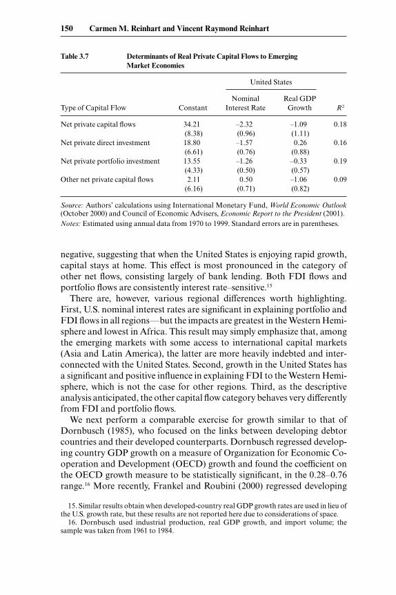
negative, suggesting that when the United States is enjoying rapid growth,capital stays at home. This effect is most pronounced in the category ofother net flows, consisting largely of bank lending. Both FDI flows andportfolio flows are consistently interest rate–sensitive.15

There are, however, various regional differences worth highlighting.First, U.S. nominal interest rates are significant in explaining portfolio andFDI flows in all regions—but the impacts are greatest in the Western Hemi-sphere and lowest in Africa. This result may simply emphasize that, amongthe emerging markets with some access to international capital markets(Asia and Latin America), the latter are more heavily indebted and inter-connected with the United States. Second, growth in the United States hasa significant and positive influence in explaining FDI to the Western Hemi-sphere, which is not the case for other regions. Third, as the descriptiveanalysis anticipated, the other capital flow category behaves very differentlyfrom FDI and portfolio flows.

We next perform a comparable exercise for growth similar to that ofDornbusch (1985), who focused on the links between developing debtorcountries and their developed counterparts. Dornbusch regressed develop-ing country GDP growth on a measure of Organization for Economic Co-operation and Development (OECD) growth and found the coefficient onthe OECD growth measure to be statistically significant, in the 0.28–0.76range.16 More recently, Frankel and Roubini (2000) regressed developing


15. Similar results obtain when developed-country real GDP growth rates are used in lieu ofthe U.S. growth rate, but these results are not reported here due to considerations of space.

16. Dornbusch used industrial production, real GDP growth, and import volume; thesample was taken from 1961 to 1984.

Table 3.7 Determinants of Real Private Capital Flows to Emerging Market Economies

United States

Nominal Real GDPType of Capital Flow Constant Interest Rate Growth R2

Net private capital flows 34.21 –2.32 –1.09 0.18(8.38) (0.96) (1.11)

Net private direct investment 18.80 –1.57 0.26 0.16(6.61) (0.76) (0.88)

Net private portfolio investment 13.55 –1.26 –0.33 0.19(4.33) (0.50) (0.57)

Other net private capital flows 2.11 0.50 –1.06 0.09(6.16) (0.71) (0.82)

Source: Authors’ calculations using International Monetary Fund, World Economic Outlook(October 2000) and Council of Economic Advisers, Economic Report to the President (2001).Notes: Estimated using annual data from 1970 to 1999. Standard errors are in parentheses.

country growth for various regional groupings against the G7 real interestrate; they found that the coefficients on real interest rates were negative andin most cases statistically significant, with the greatest interest sensitivity inthe Western Hemisphere.17

Our exercise here combines these two approaches. As shown in table 3.8,when GDP growth for the various country groupings is regressed againstU.S. growth and the short-term real interest rate, the results tend to be quiteintuitive. The sensitivity of growth to U.S. growth is highest (and statisticallysignificant) for the newly industrialized Asian economies, which dependgreatly on trade with the United States, and lowest for the remainder of Asia.For all developing countries, both of the regressors have the anticipated signsand are statistically significant. A 1 percentage point decline in U.S. growthrates reduces GDP growth for the developing countries by 0.2 percent, whilea 1 percent increase in U.S. real interest rates reduces it by 0.24 percent. De-spite strong trade links with the United States for most countries in the re-gion, U.S. growth is only marginally statistically significant for the WesternHemisphere, although the coefficient is positively signed. U.S. growth is alsosignificant for the Middle East and European developing countries. Given itshistory of relatively high levels of indebtedness and periodic debt-servicingdifficulties, it is not surprising that the U.S. real interest rate is significant andthat growth is most sensitive to interest rate fluctuations in the Western


Table 3.8 Determinants of Real GDP Growth in Emerging Market Economies

United States

Short Real Real GDPRegion/Country Constant Interest Rate Growth R2

Newly industrialized Asian economies 6.25 –0.21 0.56 0.16

(0.94) (0.23) (0.25)Developing countries 4.83 –0.24 0.20 0.23

(0.40) (0.10) (0.11)Africa 2.95 –0.14 0.05 0.03

(0.60) (0.15) (0.16)Asia 6.30 0.16 0.01 0.04

(0.67) (0.16) (0.18)Middle East and Europe 3.84 –0.52 0.43 0.17

(1.04) (0.26) (0.28)Western Hemisphere 3.73 –0.71 0.32 0.43

(0.66) (0.16) (0.17)

Source: Authors’ calculations using International Monetary Fund, World Economic Outlook(October 2000) and Council of Economic Advisers, Economic Report to the President (2001).Notes: Estimated using annual data from 1970 to 1999. Standard errors are in parentheses.

17. The coefficient for the Western Hemisphere was –0.77, compared to –0.39 for all marketborrowers.

Hemisphere; the coefficient (–0.71) is almost four times as large, in absoluteterms, as for all developing countries. Indeed, one cannot reject the hypoth-esis that a 1 percent increase in U.S. real interest rates leads to a 1 percent de-cline in growth in the region. Real U.S. interest rates are also statistically sig-nificant for the Middle East and Europe. For countries at the other end of thespectrum—the newly industrialized Asian economies, with low levels of ex-ternal debt and considerable access to private capital markets—U.S. interestrates are not significant, although the coefficient has the expected negativesign. As far as these regressions are concerned, U.S. developments have nosystematic relationship with the rest of developing Asia.18

3.4 The Consequences of Exchange Rate and Interest Rate Volatility in the North

To examine the issue of whether the volatility of interest rates and G3exchange rates has adverse consequences for cross-border capital flowsto emerging markets and growth, we split our sample into high- and low-volatility periods and conduct a set of exercises comparable to those dis-cussed in the preceeding section.

3.4.1 Background on Exchange Rate Variability in Emerging Markets

The argument that excessive volatility of G3 exchange rates imposes sig-nificant costs on emerging markets seems to rely mostly on a spendingchannel. A large swing in the dollar’s value on the foreign exchange marketin terms of the yen and the euro translates directly into changes in the com-petitiveness of countries that link their currencies to the dollar—eitherthrough a hard peg or a highly managed float. The evidence in Calvo andReinhart (2002) suggests that many developing countries fall into thatgroup. They report a widespread “fear of floating,” in that many emergingmarket currencies tend to track the dollar or the euro closely, even in casesthat are officially classified as floating.

Some sense of the stakes for emerging-market economies can be hadfrom figures 3.4 through 3.6 and table 3.9. We calculated simple annual av-erages of the absolute value of the monthly changes in the logarithms of thereal deutsche Mark/dollar and real yen/dollar exchange rates from 1970 to1999, of the percentage point change in the real U.S. treasury bill rate (onthe rationale that most developing country borrowing is denominated inU.S. dollars) from 1973 to 1999, and of the monthly changes in the loga-rithm of U.S. real personal consumption expenditure from 1970 to 1999.


18. An elegant model that broadly supports this pattern of coefficients is provided by Gertlerand Rogoff (1990). They offer a framework in which a country’s level of wealth influences theextent of agency problems in lending and, therefore, the degree of integration with the worldcapital market. As a general rule in table 3.8, regions with greater per capita wealth tend to bemore tightly linked to U.S. interest rates.

Fig

. 3.4

G3

real

exc

hang

e ra

te v

olat

ility

and

cap

ital

flow

s to

emer

ging

mar

ket e

cono

mie

s (bi

llion

s of 1

970

U.S

. dol

lars

, 197

0– 9

9):

A,N

et r

eal p

riva

te c

apit

al fl

ows;

B,N

et r

eal p

riva

te d

irec

t in

vest

men

t; C

,Net

rea

l pri

vate

por

tfol

io in

vest

men

t; D

,Oth

er n

et r

eal

priv

ate

capi

tal fl

ows

Sou

rce:

Aut

hors

’ cal

cula

tion

s us

ing

Inte

rnat

iona

l Mon

etar

y F

und

Wor

ld E

cono

mic

Out

look

(Oct

ober

200

0).

Fig

. 3.5

U.S

. rea

l sho

rt-t

erm

inte

rest

vol

atili

ty a

nd c

apit

al fl

ows t

o em

ergi

ng m

arke

t eco

nom

ies (

billi

ons o

f 197

0 U

.S. d

olla

rs, 1

973–

99):

A,N

et re

alpr

ivat

e ca

pita

l flow

s; B

,Net

real

pri

vate

dir

ect i

nves

tmen

t; C

,Net

real

pri

vate

por

tfol

io in

vest

men

t; D

,Oth

er n

et re

al p

riva

te c

apit

al fl

ows

Sou

rce:

Aut

hors

’ cal

cula

tion

s us

ing

Inte

rnat

iona

l Mon

etar

y F

und

Wor

ld E

cono

mic

Out

look

(Oct

ober

200

0).

Fig

. 3.6

U.S

. rea

l con

sum

ptio

n vo

lati

lity

and

capi

tal fl

ows t

o em

ergi

ng m

arke

t eco

nom

ies (

billi

ons o

f 197

0 U

.S. d

olla

rs, 1

970–

99)

:A

,Net

rea

l pri

vate

cap

ital

flow

s; B

,Net

rea

l pri

vate

dir

ect

inve

stm

ent;

C,N

et r

eal p

riva

te p

ortf

olio

inve

stm

ent;

D,O

ther

net

rea

lpr

ivat

e ca

pita

l flow

sS

ourc

e:A

utho

rs’ c

alcu

lati

ons

usin

g In

tern

atio

nal M

onet

ary

Fun

d W

orld

Eco

nom

ic O

utlo

ok(O

ctob

er 2

000)

.

The three figures split the sample into two states of nature: those in whichG3 exchange rate volatility is above and below the sample median (in fig.3.4), those in which U.S. interest rate volatility is above and below thesample median (in fig. 3.5), and those in which the average annual volatilityof U.S. personal consumption expenditure is above and below the median(in figure 3.6). As before, we report the volume of real capital flows by coun-try grouping and type across the sample split. As is evident from figure 3.4,the volatility of G3 exchange rates has little discernible effect on net realprivate capital flows to emerging-market economies or on any of the majorregions reported. Beneath that total, though, there are important composi-tional effects, in that both portfolio and other net capital flows step lowerwhen G3 exchange rate volatility is higher. The unchanged total is due to thefact that private direct investment moves in the opposite direction: From1970 to 1999, FDI tended to be higher in those years when G3 exchange ratevolatility was on the high side of the median.

Similar offsetting movements of FDI and portfolio and other capitalflows are evident when the sample is split according to the volatility of theU.S. short-term real interest rates, as in figure 3.5. In this case, on net, realprivate capital flows are somewhat higher when U.S. rates move more frommonth to This follows because the expansion of portfolio and other flowswhen interest rates are volatile more than makes up for a contraction inFDI. Apparently, the short-term financial transactions in portfolio andother flows are energized by interest rate volatility, even as the longer-termtransactions in FDI flag.

The total and major components of private capital flows respond moresimilarly when the sample is split according to the volatility of U.S. con-sumption spending, as seen in figure 3.6. Relatively stable personal con-sumption expenditure (PCE) growth in the United States is associated with


Table 3.9 Volatility and Foreign Real GDP Growth: Annual Rate (%), 1970–99

Degree of U.S.Consumption

Volatility

Degree ofG3 Currency

Volatility

Degree of U.S. RateVolatility

Region/Country High Low High Low High Low

Newly industrialized Asian economies 7.95 7.02 6.96 8.49 8.94 6.23

Developing countries 5.33 4.56 4.68 5.54 5.25 4.88Africa 2.42 2.75 2.73 3.12 3.44 2.30Asia 6.53 6.89 6.30 6.87 6.64 6.48Middle East and Europe 4.33 3.37 3.55 5.42 4.90 3.89Western Hemisphere 4.90 1.98 3.33 4.09 3.87 3.47

Source: Authors’ calculations using International Monetary Fund, World Economic Outlook (October2000).Note: Sample period for U.S. rate volatility is 1973 to 1999.

larger capital flows, on net, to emerging market economies, especially thosetaking the form of foreign direct and portfolio investment. To an importantextent, this may be due to the combination of a secular decline in U.S. con-sumption volatility and a secular increase in the volume of capital flows.Simply, low–consumption volatility years predominate later in the sample,when capital flows are also larger.19

Table 3.9 reports the average annual growth rates of real GDP in devel-oping countries for different splits of the data determined by the volatili-ties, in turn, of G3 exchange rates, U.S. interest rates, and U.S. consumption.As a general rule, neither G3 exchange rate volatility nor U.S. consump-tion volatility appears harmful to growth prospects in emerging marketeconomies. In both cuts of the data, high volatility is associated with about1⁄2 to 3⁄4 percentage point faster growth in developing countries, as we seewhen comparing columns (1) and (2) for G3 exchange rates or columns (5)and (6) for U.S. consumption. For some regions, particularly newly indus-trialized Asian economies, the difference is quite large. What is also appar-ent is that U.S. short-term interest rates, on average, are linked to slowereconomic growth in the developing world, with differences in growth acrossthe two regimes ranging from 3/8 to nearly 2 percentage points.

The insight that emerges from the simple model is that enforcing targetzones in the G3 currencies involves choosing a point along the trade-off be-tween lower exchange rate volatility and higher interest rate volatility.Moreover, to the extent that G3 spending is sensitive to interest rates, therewill be a corresponding trade-off between lower exchange rate volatility andhigher consumption volatility. We parsed our sample along the dimensionsof that trade-off, examining capital flows and GDP growth according to thejoint behavior of the relevant volatilities. Table 3.10 records those results.From an emerging-market perspective, G3 target zones imply moving fromthe upper right cell of each panel, where G3 currency volatility is high butU.S. interest rate of PCE volatility is low, to the lower left cell, where G3 cur-rency volatility is low but U.S. interest rate or PCE volatility is high.

With regard to the upper four panels of the table looking at the comove-ment of G3 exchange rate and U.S. interest rate volatility, net private capi-tal flows were almost $5 billion higher, on average, in those years in whichG3 exchange rates were not volatile and U.S. interest rates were. However,by considering the minor diagonals on the other three panels, it becomeclear that this is the case because a sizable decline in FDI across the two pe-riods was offset by increases in hotter-money flows—portfolio investmentand other private flows. Moreover, it would have been unwise in emerging-market economies over the past twenty-seven years to trade times when G3exchange rates were volatile but U.S. PCE growth was stable for times whenG3 exchange rates were stable but U.S. PCE growth was volatile. Across the


19. Two-thirds of the observations on PCE variability in the first half of the sample lie abovethe median calculated over the entire sample.

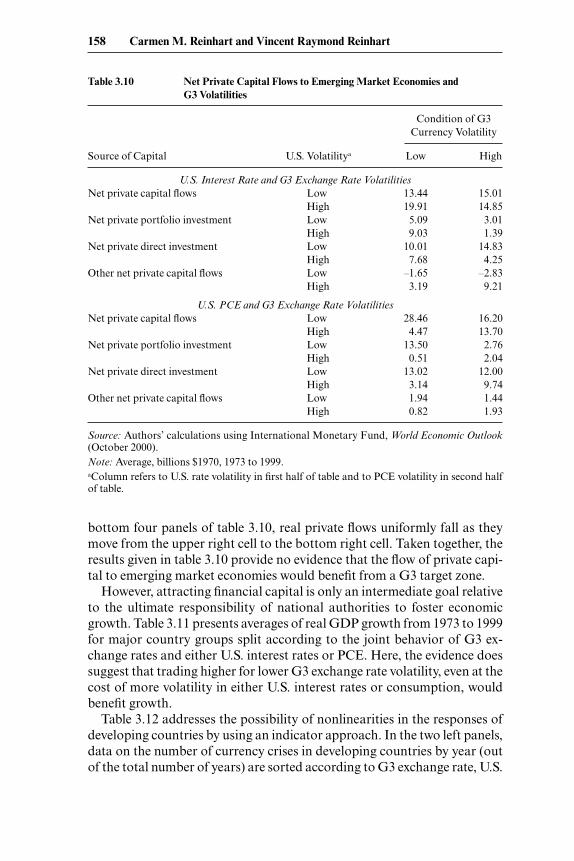
bottom four panels of table 3.10, real private flows uniformly fall as theymove from the upper right cell to the bottom right cell. Taken together, theresults given in table 3.10 provide no evidence that the flow of private capi-tal to emerging market economies would benefit from a G3 target zone.

However, attracting financial capital is only an intermediate goal relativeto the ultimate responsibility of national authorities to foster economicgrowth. Table 3.11 presents averages of real GDP growth from 1973 to 1999for major country groups split according to the joint behavior of G3 ex-change rates and either U.S. interest rates or PCE. Here, the evidence doessuggest that trading higher for lower G3 exchange rate volatility, even at thecost of more volatility in either U.S. interest rates or consumption, wouldbenefit growth.

Table 3.12 addresses the possibility of nonlinearities in the responses ofdeveloping countries by using an indicator approach. In the two left panels,data on the number of currency crises in developing countries by year (outof the total number of years) are sorted according to G3 exchange rate, U.S.


Table 3.10 Net Private Capital Flows to Emerging Market Economies and G3 Volatilities

Condition of G3Currency Volatility

Source of Capital U.S. Volatilitya Low High

U.S. Interest Rate and G3 Exchange Rate VolatilitiesNet private capital flows Low 13.44 15.01

High 19.91 14.85Net private portfolio investment Low 5.09 3.01

High 9.03 1.39Net private direct investment Low 10.01 14.83

High 7.68 4.25Other net private capital flows Low –1.65 –2.83

High 3.19 9.21

U.S. PCE and G3 Exchange Rate VolatilitiesNet private capital flows Low 28.46 16.20

High 4.47 13.70Net private portfolio investment Low 13.50 2.76

High 0.51 2.04Net private direct investment Low 13.02 12.00

High 3.14 9.74Other net private capital flows Low 1.94 1.44

High 0.82 1.93

Source: Authors’ calculations using International Monetary Fund, World Economic Outlook(October 2000).Note: Average, billions $1970, 1973 to 1999.aColumn refers to U.S. rate volatility in first half of table and to PCE volatility in second halfof table.

Table 3.12 Likelihood of the Twin Crises and G3 Volatilities

Condition of G3 Currency Volatility

Type of Crises U.S. Volatility Low High

Currency crises Lowa 0.10 0.25Higha 0.10 0.10

Banking crises Lowa 0.05 0.20Higha 0.10 0.15

Currency crises Lowb 0.10 0.25Highb 0.10 0.10

Banking crises Lowb 0.10 0.20Highb 0.05 0.15

Source: Authors’ calculations using International Monetary Fund, World Economic Outlook(October 2000).Note: Percent of the sample of above-the-median crises, 1980 to 1998.aColumn refers to U.S. rate volatility.bColumn refers to U.S. PCE volatility.

Table 3.11 Real GDP Growth in Emerging Market Economies and G3 Volatilities

Condition of G3Currency Volatility

Region U.S. Volatilitya Low High

U.S. Interest Rate and G3 Exchange Rate VolatilitiesNewly industrialized Asian economies Low 8.46 6.44

High 8.06 7.83Asia Low 8.10 6.41

High 6.89 6.12Developing countries Low 4.93 4.42

High 5.51 5.11Western Hemisphere Low 9.04 9.93

High 7.37 6.20

U.S. PCE and G3 Exchange Rate VolatilitiesNewly industrialized Asian economies Low 7.44 5.32

High 9.13 8.60Asia Low 7.91 5.41

High 6.63 7.19Developing countries Low 5.92 4.10

High 4.56 5.25Western Hemisphere Low 6.08 6.04

High 4.51 5.44

Source: Authors’ calculations using International Monetary Fund, World Economic Outlook(October 2000).Note: Average annual rate, percent, 1973 to 1999.aColumn refers to U.S. rate volatility in first half of table and to U.S. PCE volatility in secondhalf of table.

interest rate, and PCE volatility (with the crisis indicator defined accordingto the methodology in Frankel and Rose 1996, as recently updated and ex-tended to a larger country set by Reinhart 2000).20 The right panels reportsimilar calculations using the number of banking crises from the samesource. As can be seen along the minor diagonals of the four panels, yearsin which G3 exchange rate volatility was above its median and interest ratevolatility in the United States was below its median over the past eighteenyears were associated with relatively more crises in developing countries, es-pecially compared to those years when G3 currency volatility was low butU.S. interest rate volatility was high. In that sense, advocates of target zonesare correct in noting that crises are more frequent when G3 exchange ratesare more volatile. Moreover, that historical record suggests that the situa-tion can be improved upon by reducing that volatility by incurring more in-terest rate of PCE volatility in the United States.

3.4.2 Basic Tests

The difficulty in interpreting these data, whether on capital flows or GDPgrowth, is that some of the regularities observed in moving between the cellsof these contingency tables may result from systematic macroeconomicchanges rather than unique effects from the various volatilities. However,in an earlier section, we offered a simple regression that helped to explainemerging-market economies’ capital flows and GDP growth using variablesthat could be treated as exogenous to the South–U.S. interest rates and eco-nomic growth. We now ask whether G3 indicator variables have any abilityto explain the residuals to those “fundamental” regressions, and therebyput confidence bands about the estimates of the effects of interest rate andexchange rate volatility on capital flows and GDP growth.

Each block of table 3.13 corresponds to a specification in which the resid-ual from the equation explaining the capital flow concept in the columnhead is regressed against two G3 dummies (with no constant terms, as thedummies are exhaustive). Those dummies are the same we have used to splitthe data in the various exercises already reported and capture the U.S. busi-ness cycle; U.S. monetary policy; the volatilities of U.S. real short-term rates,G3 exchange rates, and U.S. consumption growth; currency crises; andbanking crises.21 In general, a statistically significant coefficient would indi-cate that a G3 factor exerted an additional influence beyond that containedin U.S. interest rates and income. As to G3 target zones in particular, thereappears to be no significant effect on average of episodes of higher vola-tilities by either measure for topline net capital flows. Taken literally—no doubt too literally—this would indicate there is no particular cost to


20. The results are similar when one employs the methodology of Kaminsky and Reinhart(1999).

21. Thus, there are twenty-eight regressions reported in the table corresponding to four mea-sures of capital flows and seven different sets of states of nature.

Table 3.13 Can “Excess” Real Capital Flows Be Explained by G3 Factors?

Net Private Capital Flows

Type of Factor Total Direct Investment Portfolio Other

U.S. business cycleExpansion 0.44 0.69 0.61 –0.88

(2.72) (2.14) (1.39) (1.98)Recession –1.03 –1.61 –1.41 2.06

(4.16) (2.14) (2.13) (1.98)U.S. monetary policy

Tightening –1.78 0.42 –0.44 –1.78(3.58) (2.85) (1.86) (2.62)

Easing 1.19 –0.28 0.29 1.18(2.92) (2.32) (1.52) (2.14)

Volatility of U.S. real short-term ratesa

High 2.40 –2.53 1.58 3.28(3.49) (2.51) (1.77) (2.37)

Low 0.02 4.47 –0.18 –4.30(3.36) (2.42) (1.71) (2.29)

Volatility of G3 exchange rates

High 0.85 3.04 –0.92 –1.34(3.11) (2.32) (1.59) (2.27)

Low –0.97 –3.47 1.05 1.53(3.33) (2.48) (1.70) (2.42)

Volatility of U.S. consumption

High –4.93 –3.15 –2.76 1.06(2.81) (2.31) (1.42) (2.28)

Low 5.63 3.61 3.16 –1.21(3.00) (2.47) (1.52) (2.44)

Currency crisesb

High 1.44 1.66 3.34 –3.61(4.37) (2.76) (2.04) (2.55)

Low 5.25 4.22 1.38 –3.61(5.12) (3.23) (2.39) (2.99)

Banking crisesc

High 2.34 1.99 3.82 –3.55(4.62) (2.91) (2.11) (2.69)

Low 3.83 3.57 1.07 –0.84(4.87) (3.07) (2.22) (2.83)

Source: Authors’ calculations using International Monetary Fund, World Economic Outlook(October 2000) and Council of Economic Advisers, Economic Report to the President (2001).Notes: Relationship of the residual from the capital flow fundamentals equations to G3dummy variables from 1970 to 1999. Standard errors are in parentheses.aEstimated from 1973 to 1999.bEstimated from 1980 to 1998.cEstimated from 1980 to 1998.

making real interest rates more volatile, but there is also no particular bene-fit in damping G3 exchange rate volatility. This statistical evidence ultimatelydiffers little from the theoretical analysis; from the perspective of emerging-market economies, the case for limiting G3 exchange rate volatility is notproven. A similar analysis across regional aggregates, not included here dueto considerations of space, provides no reason to question that judgment.

We performed a similar exercise to see if episodes of either volatile G3 ex-change rates or U.S. real interest rates exerted a systematic influence on thegrowth of output in major emerging-market areas. Those results, reportedin table 3.14, tell a similar story. Across the six areas examined, none of thedummy variables related to the various volatilities differed significantlyfrom zero. Taken together, the evidence suggests that advocates of G3 tar-get zones have to identify another mechanism by which financial marketvolatility in the industrial countries impinges on their neighbors to theSouth beyond that expected through the flows of trade (with their associ-ated effects on income) or capital.

3.5 Concluding Remarks

In this paper, we have attempted to analyze and quantify how develop-ments in the exchange rate arrangements of the G3 countries influenceemerging market economies. The debate on G3 target zones should be placedin the broader context of the ongoing debate on exchange rate arrangementsin emerging-market economies, which often hinge on credibility. The advo-cates for dollarization, for instance, argue that a nation with an uneven his-tory of commitment to low inflation can import the reputation of the centralbank of the anchor currency. For the issue at hand, however, there are no ob-vious bonuses to smaller countries should G3 central banks damp the fluc-tuations of their currencies—and, as discussed in Rogoff (2001), the benefitsto developed countries are limited at best. This also implies that the directbenefits to emerging-market economies should stem only from the lessenedvolatility of their trade-weighted currencies. However, as Rose (2000) pointsout, the benefits of reduced exchange rate variability on trade flows, at least,are small compared to those of adopting a common currency.

This is also the place to discuss the limitations to our analysis. In partic-ular, our use of linear, or nearly linear, models may understate the conse-quences of variability in interest rates and exchange rates. To the extent thathigh world interest rates trigger balance sheet problems in emerging mar-kets, the consequences of the trade-off implied by a target zone may be con-siderable. Indeed, one repeated message of this paper is that emerging-mar-ket economies are different from their industrial brethren, having alreadysurrendered a high degree of autonomy in their monetary policies, oftenpricing their goods in foreign—not local—currencies, and being vulnerableto sudden exclusion from world financial markets.


Table 3.14 Can “Excess” Real GDP Growth Be Explained by G3 Factors?

Newly MiddleIndustrialized Developing East and Western

Type of Factor Asia Countries Africa Asia Europe Hemisphere

U.S. business cycleExpansion 8.24 6.07 2.42 –6.82 –0.23 0.69

(3.02) (2.26) (1.53) (1.97) (0.68) (0.69)Recession 6.54 –0.17 –0.86 1.46 0.54 0.87

(4.62) (3.45) (2.34) (3.01) (1.04) (1.06)U.S. monetary policy

Tightening 4.12 4.37 0.29 –7.14 –1.23 –0.47(3.91) (3.11) (2.06) (2.76) (0.85) (0.87)

Easing 10.14 4.08 2.20 –2.47 0.82 1.55(3.19) (2.54) (1.68) (2.25) (0.70) (0.71)

Volatility of U.S. real short-term ratesa

High 9.74 0.66 2.36 –0.30 –0.85 –0.50(4.01) (2.86) (2.07) (2.51) (0.77) (0.77)

Low 7.06 8.76 0.93 –9.37 –0.26 0.88(3.87) (2.76) (1.99) (2.42) (0.74) (0.74)

Volatility of G3 exchange rates

High 7.67 6.03 –0.40 –4.98 –0.34 0.46(3.47) (2.64) (1.73) (2.46) (0.78) (0.79)

Low 7.80 2.10 3.54 –3.60 0.39 1.05(3.71) (2.82) (1.84) (2.63) (0.83) (0.85)

Volatility of U.S. consumption

High 2.12 1.31 –1.24 –3.83 0.19 0.98(3.10) (2.57) (1.64) (2.46) (0.78) (0.79)

Low 14.15 7.50 4.50 –4.92 –0.22 0.46(3.32) (2.75) (1.75) (2.63) (0.84) (0.85)

Currency crisesb

High 6.44 3.83 3.03 –7.35 –0.89 0.09(4.93) (3.10) (2.49) (2.95) (0.76) (0.83)

Low 15.99 10.33 4.23 –5.47 –0.48 0.40(5.78) (3.64) (2.92) (3.46) (0.89) (0.97)

Banking crisesc

High 9.30 4.70 4.24 –6.76 –0.71 0.12(5.39) (3.36) (2.61) (3.11) (0.80) (0.87)

Low 11.75 8.64 2.76 –6.33 –0.73 0.34(5.68) (3.55) (2.75) (3.28) (0.84) (0.92)

Source: Authors’ calculations using International Monetary Fund, World Economic Outlook (October2000) and Council of Economic Advisers, Economic Report to the President (2001).Notes: Relationship of the residual from the real GDP growth fundamentals equations to G3 dummyvariables from 1970 to 1999. Standard errors are in parentheses.aEstimated from 1973 to 1999.bEstimated from 1980 to 1998.cEstimated from 1980 to 1998.

Appendix

Determinants of Real Private Capital Flows to EmergingMarket Economies

United States

Region/Country Nominal Interest Rate Real GDP R 2

AfricaNet private capital flows 0.21 0.04 0.06

(0.17) (0.19)Net private direct investment –0.07 0.00 0.15

(0.03) (0.04)Net private portfolio investment –0.09 0.04 0.21

(0.04) (0.05)Other net private capital flows 0.37 0.00 0.15

(0.18) (0.20)Asia and crisis countries

Net private capital flows 0.05 –0.42 0.05(0.34) (0.39)

Net private direct investment –0.12 –0.02 0.15(0.06) (0.06)

Net private portfolio investment –0.25 –0.05 0.13(0.13) (0.15)

Other net private capital flows 0.43 –0.35 0.18(0.25) (0.29)

Other Asian emerging marketsNet private capital flows –0.26 –0.06 0.03


(0.27) (0.31)Net private portfolio investment –0.04 –0.04 0.03

(0.05) (0.06)Other net private capital flows 0.42 –0.09 0.11

(0.25) (0.28)Middle East and Europe

Net private capital flows –1.68 –0.25 0.33(0.46) (0.54)

Net private direct investment –0.08 0.08 0.11(0.07) (0.08)

Net private portfolio investment 0.02 –0.06 0.01(0.12) (0.14)

Other net private capital flows –1.63 –0.27 0.39(0.40) (0.46)

Western HemisphereNet private capital flows 0.04 –0.29 0.01


(0.27) (0.32)Net private portfolio investment –0.73 –0.21 0.20

(0.28) (0.32)Other net private capital flows 1.18 –0.21 0.27

(0.40) (0.46)

Source: Authors’ calculations using International Monetary Fund, World Economic Outlook (October2000) and Council of Economic Advisers, Economic Report to the President (2001).Note: Estimated using annual data from 1970 to 1999. Standard errors are in parentheses.

References

Borensztein, Eduardo, and Carmen M. Reinhart. 1994. The macroeconomic deter-minants of commodity prices. IMF Staff Papers 41 (2): 236–60.

Calvo, Guillermo, Leonardo Leiderman, and Carmen M. Reinhart. 1993. Capital in-flows and the real exchange rate in Latin America: The role of external factors.IMF Staff Papers 40 (1): 108–50.

Calvo, Guillermo A., and Carmen M. Reinhart. 2002. Fear of floating. QuarterlyJournal of Economics CXVII (2): 379–408.

Chu, Ke-Young, and Thomas K. Morrison. 1984. The 1981–82 recession and non-oil primary commodity prices. IMF Staff Papers 31 (1): 93–140.

Clarida, Richard H. 2000. G3 exchange rate relationships: A recap of the record anda review of proposals for change. Princeton Essays in International Economics no.219. Princeton University, Department of Economics, International EconomicsSection.

Dominguez, Kathryn M., and Jeffrey A. Frankel. 1993. Does foreign exchange in-tervention matter? The portfolio effect. American Economic Review 83:1356–59.

Dornbusch, Rudiger. 1985. Policy and performance links between LDC debtors andindustrial nations. Brookings Papers on Economic Activity, Issue no. 2:303–56.

Fernandez-Arias, Eduardo. 1996. The new wave of private capital inflows: Push orpull? Journal of Development Economics 48:389–418.

Frankel, Jeffrey A., and Andrew Rose. 1996. Currency crashes in emerging markets:An empirical treatment. Journal of International Economics 41:351–66.

Frankel, Jeffrey A., Sergio Schmukler, and Luis Servén. 2001. Verifiability and thevanishing intermediate exchange rate regime. In Policy challenges in the next mil-lennium, ed. Susan Collins and Dani Rodrik, 59–108. Washington, D.C.: Brook-ings Institution.

Frankel, Jeffrey A., and Nouriel Roubini. 2000. The role of industrial country poli-cies in emerging market crises. paper prepared for the NBER conference on Eco-nomic and Financial Crises in Emerging Market Economies, 19–21 October,Woodstock, Vt.

Gertler, Mark, and Kenneth Rogoff. 1990. North-south lending and endogenousdomestic capital market inefficiencies. Journal of Monetary Economics 26:245–66.

Goldstein, Morris. 1999. Safeguarding prosperity in a global financial system: Reportof an independent task force of the Council on Foreign Relations. New York: Coun-cil on Foreign Relations.

Holtham, Gerald H. 1988. Modeling commodity prices in a world macroeconomicmodel. In International Commodity Market Models and Policy Analysis, ed. OrhanGüvenen, 221–58. Boston: Kluwer Academic Publishers.

International Monetary Fund. 1999. Direction of trade statistics. Washington, D.C.:International Monetary Fund.

———. 2000a. International financial statistics. Washington, D.C.: InternationalMonetary Fund.

———. 2000b. World Economic Outlook database. Available at [http://www.imf.org].Kaminsky, Graciela L., and Karen K. Lewis. 1996. Does foreign exchange interven-

tion signal future monetary policy? Journal of Monetary Economics 37:285–312.Kaminsky, Graciela L., and Carmen M. Reinhart. 1999. The twin crises: The causes

of banking and balance-of-payments problems. American Economic Review 89: 473–500.

———. 2001. Bank lending and contagion: Evidence from the Asian crisis. In Re-gional and global capital flows: Macroeconomic causes and consequences, ed. T. Itoand A. Krueger, 73–116. Chicago: University of Chicago Press.

Kaminsky, Graciela L., and Sergio Schmukler. 2001. Emerging market instability:


Do sovereign ratings affect country risk and stock returns? World Bank. Mimeo-graph.

Marquez, Jaime. 1990. Bilateral trade elasticities. The Review of Economics and Sta-tistics 72 (1): 70–77.

McKinnon, Ronald. 1984. An international standard for monetary stabilization.Washington, D.C.: Institute for International Economics.

———. 1997. The rules of the game. Cambridge: MIT Press.Reinhart, Carmen M. 1995. Devaluation, relative prices, and trade. IMF Staff Pa-

pers 42 (2): 290–310.———. 2000. Sovereign credit ratings before and after financial crises. World Bank

Economic Review, forthcoming.Rogoff, Kenneth. 2001. On why not a global currency. American Economic Review

91 (2): 243–47.Rose, Andrew K. 2000. One money, one market: Estimating the effect of common

currencies on trade. Economic Journal 15.Williamson, John. 1986. Target zones and the management of the dollar. Brookings

Papers on Economic Activity, Issue no. 1:165–74.

Comment Joshua Aizenman

This interesting paper investigates an issue of great importance to emergingmarkets—the welfare effect of attempts to reduce the exchange rate volatil-ity among the G3 currencies. My discussion will start with an overview ofthe main message of the paper and will conclude with several remarks re-garding the robustness of the arguments advanced in it.

Overview

The Goal

The purpose of the paper is to examine the welfare effect, from an emerg-ing-market perspective, of reducing the G3 currencies’ variability. It ex-plores the various channels of North-South transmission and analyzes thelink between the G3 exchange rate and interest rate volatility, and economicgrowth in developing countries.

The Background

Using target zones as a mechanism for reducing the volatility of the G3currencies has been advocated by various economists, including McKin-non, Williamson, Clarida, and others. These proposals focused mostly onthe Organization for Economic Cooperation and Development (OECD).Little attention was given to the implications of adopting the target zone


Joshua Aizenman is professor of economics at the University of California, Santa Cruz, anda research associate of the National Bureau of Economic Research.

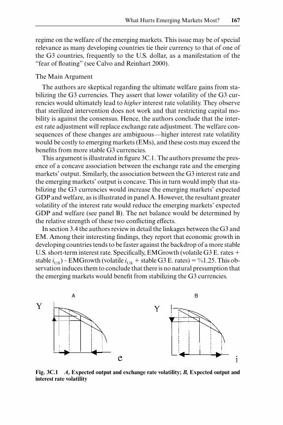
regime on the welfare of the emerging markets. This issue may be of specialrelevance as many developing countries tie their currency to that of one ofthe G3 countries, frequently to the U.S. dollar, as a manifestation of the“fear of floating” (see Calvo and Reinhart 2000).

The Main Argument

The authors are skeptical regarding the ultimate welfare gains from sta-bilizing the G3 currencies. They assert that lower volatility of the G3 cur-rencies would ultimately lead to higher interest rate volatility. They observethat sterilized intervention does not work and that restricting capital mo-bility is against the consensus. Hence, the authors conclude that the inter-est rate adjustment will replace exchange rate adjustment. The welfare con-sequences of these changes are ambiguous—higher interest rate volatilitywould be costly to emerging markets (EMs), and these costs may exceed thebenefits from more stable G3 currencies.

This argument is illustrated in figure 3C.1. The authors presume the pres-ence of a concave association between the exchange rate and the emergingmarkets’ output. Similarly, the association between the G3 interest rate andthe emerging markets’ output is concave. This in turn would imply that sta-bilizing the G3 currencies would increase the emerging markets’ expectedGDP and welfare, as is illustrated in panel A. However, the resultant greatervolatility of the interest rate would reduce the emerging markets’ expectedGDP and welfare (see panel B). The net balance would be determined bythe relative strength of these two conflicting effects.

In section 3.4 the authors review in detail the linkages between the G3 andEM. Among their interesting findings, they report that economic growth indeveloping countries tends to be faster against the backdrop of a more stableU.S. short-term interest rate. Specifically, EMGrowth (volatile G3 E. rates �stable iU.S.) – EMGrowth (volatile iU.S. � stable G3 E. rates) � %1.25. This ob-servation induces them to conclude that there is no natural presumption thatthe emerging markets would benefit from stabilizing the G3 currencies.


A B

Fig. 3C.1 A, Expected output and exchange rate volatility; B, Expected output andinterest rate volatility

Response

Is There a Trade-Off Between Interest Rate Volatility and Exchange Rate Volatility for the G3?

The logic of the paper presumes the existence of a trade-off between in-terest rate and exchange rate volatility for the G3. With such a trade-off, fig-ure 3C.1 illustrates the ambiguity of the welfare effects attributed to greaterexchange rate stability. However, no evidence is presented to support thispresumption. The existing literature provides us with little guidance regard-ing this issue. In fact, several contributions are skeptical about this trade-off.For example, Flood and Rose (1995) failed to find such a trade-off, report-ing, “The graphs indicate that there is no substantial tradeoff between ex-change rate volatility and the volatility of (domestic) interest rate” (Floodand Rose 1995, 17). A recent update of this study is summarized by Jeanneand Rose (1999), who found that macroeconomic fundamentals do not ex-hibit regime-varying volatility. These authors advance a possible interpreta-tion for these findings, focusing on the impact of the entry of noise traders tothe market. Accordingly, a pure float with an endogenous number of noisetraders may give rise to multiple equilibria. The same macrofundamentalsare consistent with low exchange rate volatility and a low number of noisetraders, or high exchange rate volatility and a high number of noise traders.The multiplicity follows from the observation that noise traders affect the al-location of risk in two ways—they create risk, and they allow for deeper risksharing. The ultimate impact of the entry of noise traders on the risk pre-mium is ambiguous. Jeanne and Rose illustrate that for certain configura-tions in which two equilibria exist, the inefficient one is associated with highexchange rate volatility. In that equilibrium, all noise traders are active. Theirmodel provides a nice setup for the multiple equilibrium hypothesis (Eichen-green and Wyplosz 1993). In such an economy, a target zone may eliminatethe inefficient equilibrium by restricting the feasible range of exchange ratevolatility. In this case there is a “free lunch,” in the sense that there is notrade-off between exchange rate volatility and interest rate volatility—thegood equilibrium is associated with lower exchange rate volatility as well aswith a lower risk premium and lower interest rate volatility.

This argument may be restated in terms of the earlier literature dealingwith exchange rate regimes. If most of the shocks are nominal (as will be thecase, for example, with an unstable demand for money), greater fixity of theexchange rate may be associated with lower interest rate volatility, if thesupply of money was allowed to adjust to the shocks affecting the demandfor money.

Interpreting the Empirical Facts

The empirical discussion dealing with the interest rate–monetary policycycle is very interesting and illuminating. The results dealing with the as-


sociation between the North volatility and regional GDP and capital flowsleave one in doubt. The methodology of comparing the flows of capitaland the GDP between periods of relatively stable and unstable interest andexchange rates is useful in motivating the welfare questions, yet it does notallow one to fully assess the impact of policies. Specifically, there are nocontrols for “level” variables that may explain the capital flows and theGDP. Without controlling for all the level variables that may account forcapital flows and the GDP, little can be inferred about the pure effect ofvolatility.

On the Association between Exchange Rate Volatility and the Gross Domestic Product

The presumption of the paper about the negative effect of exchange ratevolatility on the gross domestic product (GDP) has been subject to recent de-bate. The earlier Flood and Rose (1995) contribution found a weak trade-offbetween exchange rate and output volatility. Recently, however, Levy-Yeyatiand Sturzenegger (2001) report that for developing countries, less flexible ex-change rate regimes are strongly associated with both slower growth andgreater output volatility. For industrial countries, different exchange rateregimes do not appear to have any significant impact on growth.

To sum up, this paper is an interesting contribution. It raises several im-portant questions, cautioning us that the welfare effects of attempts to sta-bilize the G3 on the emerging markets are ambiguous. Resolving theseambiguities requires further investigation.

References

Calvo, Guillermo A., and Carmen M. Reinhart. 2000. Fear of floating. QuarterlyJournal of Economics, forthcoming.

Eichengreen, Barry, and Charles Wyplosz. 1993. The unstable EMS. Brookings Pa-pers on Economic Activity, Issue no. 1:51–124.

Flood, Robert, and Andrew Rose. 1995. Fixing exchange rates: A virtual quest forfundamentals. Journal of Monetary Economics 36 (1): 3–37.

Jeanne, Olivier, and Andrew K. Rose. 1999. Noise trading and exchange rateregimes. Quarterly Journal of Economics, forthcoming.

Levy-Yeyati, Eduardo, and Federico Sturzenegger. 2001. To float or to trail: Evi-dence on the impact of exchange rate regimes. Universidad Torcuato Di Tella,Department of Economics. Unpublished Manuscript.

Discussion Summary

Michael P. Dooley remarked that there is no convincing empirical evidencefor the existence of a trade-off between interest rate and exchange ratevolatility and gave support to the authors’ view that monetary policy wouldbe the only tool for supporting a G3 target zone.


Richard Portes made reference to “the balloon analogy” for describingthe volatility trade-off. He questioned the paper’s dismissal of sterilized in-tervention as a way of enforcing a target zone and pointed to empirical ev-idence suggesting that foreign exchange intervention may be effective, atleast over certain periods of time.

Robert Flood pointed to the asymmetries of crisis models data and em-phasized the importance of unconstrained estimation in order to take ac-count of skewness in the data.

Jeffrey Shafer made a reference to the European economies during the1980s and argued that there is no observed trade-off between exchange rateand interest rate volatility. He questioned, however, whether soft targetzones as opposed to fixed rates would be sufficient to meet the goals of a G3target zone.

Morris Goldstein made a reference to earlier literature and noted that bet-ter bottom-line growth and inflation performance is not a likely outcome oftarget zones. Thus, the G3 countries would be unwilling to enter such an ex-change rate arrangement, and even if they did, weaker G3 economic per-formance would not be of any help to emerging market economies.

Andrew Rose remarked that no exchange rate model seems to work well,at least not in the short run, and, therefore, even though a trade-off betweenexchange rates and interest rates seems to exist, this trade-off is hard toquantify. Martin Eichenbaum pointed out that as long as there is no clearunderstanding of what drives exchange rates, the idea of using monetarypolicy as a tool for steering exchange rates seems problematic. Dooleynoted that doing nothing because of the lack of consensus regarding the“right” exchange rate model seems problematic as well.

Jeffrey A. Frankel noted that exchange rates are not always tightly linkedto fundamentals and that sterilized intervention has been effective in thepast. However, he added, it would be impossible to commit persistent in-tervention to maintain a target zone goal since a key element for effectivesterilized intervention is sparing use of the intervention tool.

Vincent Raymond Reinhart remarked that he was sympathetic to thepoint made by Dooley regarding the lack of empirical evidence for a trade-off between exchange rates and interest rates and agreed that the assertionof such a trade-off is the weak part of the paper. He noted, in response toGoldstein, that the authors had avoided references to earlier literature,given that the focus of the paper is on emerging market economies. He re-marked that even though it is indeed possible to achieve an anchoring ofexchange rate expectations under various regimes, the necessary element iscredibility; that is, the imposition of a target zone itself is not sufficient.With respect to the issue of the effectiveness of sterilized foreign exchangeintervention, Reinhart noted that it is important to distinguish betweeneffectiveness during regimes and effectiveness during episodes.


Preventing Currency Crises in Emerging Markets

Documents

Transcript of Preventing Currency Crises in Emerging Markets