Accepted Manuscript

Title: The Cobweb, Borrowing and Financial Crises

Authors: Pasquale Commendatore, Martin Currie

PII: S0167-2681(07)00002-9DOI: doi:10.1016/j.jebo.2006.05.008Reference: JEBO 2053

To appear in: Journal of Economic Behavior & Organization

Received date: 4-1-2005Revised date: 16-12-2005Accepted date: 8-5-2006

Please cite this article as: Commendatore, P., Currie, M., The Cobweb, Borrowingand Financial Crises, Journal of Economic Behavior and Organization (2007),doi:10.1016/j.jebo.2006.05.008

This is a PDF file of an unedited manuscript that has been accepted for publication.As a service to our customers we are providing this early version of the manuscript.The manuscript will undergo copyediting, typesetting, and review of the resulting proofbefore it is published in its final form. Please note that during the production processerrors may be discovered which could affect the content, and all legal disclaimers thatapply to the journal pertain.

peer

-005

8971

8, v

ersi

on 1

- 1

May

201

1Author manuscript, published in "Journal of Economic Behavior & Organization 66, 3-4 (2008) 625"

DOI : 10.1016/j.jebo.2006.05.008

Acce

pted

Man

uscr

ipt

The Cobweb, Borrowing and Financial Crises

Pasquale Commendatore� and Martin Currie*

� University of Naples ‘Federico II’

* School of Social Sciences, University of Manchester, UK

Abstract

Studies of non-linear cobweb models have failed to address a fundamental issue:

whether the complex dynamical behavior displayed by such models is consistent

with the survival of producers. This paper shows that where borrowing is

unconstrained, as is implicitly assumed in standard cobweb models, borrowing

results in financial crises. Incorporating constraints on borrowing is needed to

salvage cobweb models. Industry performance (in terms both of profitability and of

the incidence of bankruptcies) is highly sensitive to the nature of such credit

restrictions.

JEL classification code: E32

Keywords: cobweb; economic dynamics; financial capital; bankruptcy.

Corresponding author:

Pasquale Commendatore

University of Naples, Dipartimento di Teoria Economica e Applicazioni, Via

Rodinò 22, 80138 Napoli, Italy.

E-mail: commenda@unina.it

Tel: +39 081 253 7447

Fax: +39 081 253 7454

** The authors are grateful to Richard Day, Cars Hommes, Ingrid Kubin, Ian Steedman and

Trevor Young and to anonymous referees for comments on earlier versions.

Page 1 of 30

peer

-005

8971

8, v

ersi

on 1

- 1

May

201

1

Acce

pted

Man

uscr

ipt

1

The Cobweb, Borrowing and Financial Crises

1. Introduction

Since their introduction in the 1930s to explain fluctuations in agricultural production and

prices in terms of sequential production readjustments, cobweb models have played a pivotal

role in developments in economic dynamics. In the standard model, firms in a competitive

industry produce a single homogeneous product; there is a well-defined production period,

with the producers’ activities being synchronized; producers base decisions on price

expectations; and the market-clearing product price is established instantaneously at the end

of each period. With the sole inter-temporal link being via price expectations, particular

attention has been devoted to their formation. Indeed, it was in the context of cobweb models

that adaptive expectations, rational expectations, expectations based on the mean of all past

prices and heterogeneous expectations were first analyzed.

It is, however, curious and regrettable that in a context the very essence of which is that

production takes time, very little attention has been paid to how producers finance their

production activities and to the possibility of their becoming bankrupt. Typically it is

assumed implicitly that producers can borrow or lend any amount at a given market rate of

interest determined by the overall state of the economy. Certainly a ‘perfect’ financial capital

market is a powerful simplification frequently invoked by economic theorists. In a cobweb

model, it seemingly enables theorists to dispense with financial constraints on producer

behavior and to concentrate on technological constraints. But it can be a very misleading

simplification. Indeed, assuming that producers can borrow any amount at a given interest

rate not only does not rule out bankruptcy but makes it particularly likely. Nor is bankruptcy

ruled out by assuming that producers pay for inputs at the end of the production period. To

Page 2 of 30

peer

-005

8971

8, v

ersi

on 1

- 1

May

201

1

Acce

pted

Man

uscr

ipt

2

put the matter starkly, the possibility of bankruptcy is necessarily eliminated only if

producers rely exclusively on their own financial capital to pay for inputs in advance.

Section 2 sets out the assumptions of our model. Section 3 examines the case where

producers can borrow or lend freely at a given interest rate. Looking beyond the usual

treatment of the dynamical behavior of price reveals a fundamental problem: borrowing

results in bankruptcy. However, this paper is not simply intended as a challenge to standard

non-linear cobweb models. In Section 4, following a brief consideration of the case where

firms rely exclusively on their own financial capital, we explore the implications of banks

limiting what they are prepared to lend to producers. We examine the cases where borrowing

limits depend on the values of durable assets available for use as collateral and where they

depend on producers’ financial wealth levels.

2. Assumptions

There are N units of a homogeneous durable asset, denoted by L, that is specific to the

industry and in perfectly inelastic supply (akin to Ricardian land). Since the ownership and

use of 1 (and only 1) unit of L is required for participation in the industry,1 there are, in any

period, N producers, where N is sufficiently large so that each acts as if a price-taker for the

product. Producers can acquire other inputs, but they must pay for these at the outset of the

well-defined production period using their own financial capital, possibly supplemented by

borrowed funds. At the beginning of period t (before entering into any commitments for the

ensuing period), the representative firm’s total wealth is

t t tW F V= + (1)

1 This asset could, for example, be land or a farm. With appropriate (re-)interpretations of what follows, it could

be a transferable license or permit required for participating in the industry.

Page 3 of 30

peer

-005

8971

8, v

ersi

on 1

- 1

May

201

1

Acce

pted

Man

uscr

ipt

3

where tF is its net financial wealth and 0tV ≥ is the market value of its unit of L. The firm’s

output for the tth period is

,t f v tq q q= + (2)

where 0fq > is the output per period that would result from using solely its unit of L and

where any extra output, , 0v tq ≥ , is achieved by the purchase of additional inputs. The cost

function, which is invariant over time, is

( ), ,v t v tc q qα= (3)

where 1α > , so marginal cost is increasing. The firm’s net borrowing for period t is

,t v t tB q Fα= − (4)

where Bt < 0 implies having bank deposits on which interest is received. The interest rate, r,

on a loan for the duration of the production period is determined by the overall state of the

economy and is invariant over time. The firms in the industry earn the same rate r on any

bank deposits, so that r constitutes the marginal opportunity cost of the use of own funds in

financing the production process.

Producers are motivated by the accumulation of wealth. At the beginning of period t,

subject to any financial capital constraint, the representative firm maximizes its expected

financial wealth at the beginning of period ( )1t + or, equivalently, maximizes its expected

profit for period t. The firm’s expected price for the output of period t, etp , is based on

adaptive expectations,

( )1 1 1e e et t t tp p p pγ− − −= + − (5)

where 0 1γ< ≤ is the price expectations adjustment speed, with 1γ = constituting naïve

expectations. Expected profit for period t is

Page 4 of 30

peer

-005

8971

8, v

ersi

on 1

- 1

May

201

1

Acce

pted

Man

uscr

ipt

4

( ) ,1e et t t v tp q r qαπ = − + . (6)

This definition of expected profit allows for the opportunity cost of own funds used to

finance production but does not take account of the opportunity cost of the funds tied up in

ownership of L. Once the producer is committed to participation in the industry in the current

period, the cost of ownership of L constitutes a sunk cost, and etπ amounts to an expected

quasi-rent accruing to the ownership of L.

Output is sold at the end of the period. For simplicity, we assume that the total

expenditure, E, on the product of this industry is given and invariant over time, implying a

unit elastic product demand curve. The market-clearing price, established instantaneously, is

tt

Ep

Nq= (7)

so that ( )0 t fp p E Nq< ≤ ≡� . Since total revenue is invariant, the realized profit per firm is

a strictly monotonically declining function of output:

( ) ( ), ,1 1t t t v t v tp q r q r qα απ π= − + = − +� (8)

where E Nπ ≡� is the maximum profit achieved when each firm produces the minimum

output fq . The firm’s income for period t is

t t ty rF π= + . (9)

Its financial wealth at the end of the period is

( )1 1t t t t tF F y r F π+ = + = + + . (10)

The simplest assumption that captures the notion that the market value of 1 unit of L depends

on the long-term profitability of its ownership is that it is given by the present value of the

receipt in perpetuity of the mean of the representative producer’s past profits. That is,

Page 5 of 30

peer

-005

8971

8, v

ersi

on 1

- 1

May

201

1

Acce

pted

Man

uscr

ipt

5

( )10

11

t

tVr t τ

τπ+

=

=+ � (11)

subject to 1 0tV + ≥ . The representative firm’s total wealth at the beginning of the next

production cycle is then 1 1 1t t tW F V+ + += + .

3. Unconstrained Borrowing

Suppose initially that firms can borrow any amount at the going market interest rate.

Maximizing expected profit requires that marginal cost equal the expected price:

( ) 1,1 e

v t tr q pαα −+ = . (12)

From (2) and (12),

( )1

1,

et f v t f tq q q q p α ψ−= + = + (13)

where ( )1

11 r αψ α −−= +� �� � . Using (5), (7) and (13) yields the map f:

( )1 1 1

11

( ) (1 )e e et t t

ef t

Ep f p p

N q p α

γγψ

− −

−−

= = − +� �

+� �� �

. (14)

Given an initial expected price 0ep , the future time path of expected price is uniquely

determined by (14). The time paths of tq , tp and tπ are determined uniquely from that of

etp . With an appropriate initial condition, the time path of tV can be determined from that of

tπ . The decomposition that results from unconstrained borrowing means that the time paths

of etp , tq , tp , tπ and tV do not depend on the initial financial wealth, 0F . In contrast, the

time paths for tB , ty , tF , and tW depend on 0F .

A fixed point for the map f corresponds to a stationary state, where the representative

producer is maximizing (expected) profit on the basis of a price expectation that is being

Page 6 of 30

peer

-005

8971

8, v

ersi

on 1

- 1

May

201

1

Acce

pted

Man

uscr

ipt

6

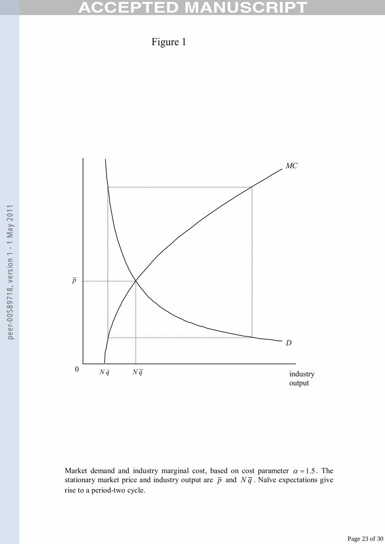
realized. The stationary values ( ), ,vp q q satisfy (i) ep p= , (ii) 1

1f v fq q q q pα ψ−= + = + ,

and (iii) N q p E= . Fig. 1 shows p and the corresponding industry output, N q . The

stationary profit, ( )1 0vr qαπ π= − + >� , constitutes a return to the ownership of L. In a

thorough-going stationary state, V rπ= and pure profit (taking account of the opportunity

cost of the wealth tied up in the ownership of L) is zero. In a stationary state, everything is

stationary except for financial wealth, bank deposits and income.

The fixed point is locally stable if ( )1 1f p′− < < , where ( )f p′ denotes the first

derivative of f evaluated at the fixed point. Expressing it in terms of vq and q confirms that

( ) 1f p′ < :

( )( ) 1 1

1vq

f pq

γγα

′ = − − <−

. (15)

Therefore, the fixed point is stable if ( ) 1f p′ > − , that is, if

( )( )2 1vq q γ α γ< − − . (16)

With naïve expectations, f is strictly monotonically decreasing: the higher is 1etp − , the higher

is 1tq − and the lower is 1e

t tp p− = . The system is attracted either to the fixed point (where

1vq q α< − ) or to a period-two cycle (where 1vq q α> − ). Fig. 2(a), based on 1.5α = and

1γ = , shows the map f corresponding to Fig. 1: the fixed point is repelling and the system is

attracted to the depicted period-two cycle.2 With adaptive price expectations, the possible

long-term behaviors are considerably enriched. Fig. 2(b), based on 1.075α = and 0.4γ = ,

2 All diagrams and simulations assume 1fq = , 0.1r = , 1000N = and 5000E = . All simulations assume

0 0.99ep p= .

Page 7 of 30

peer

-005

8971

8, v

ersi

on 1

- 1

May

201

1

Acce

pted

Man

uscr

ipt

7

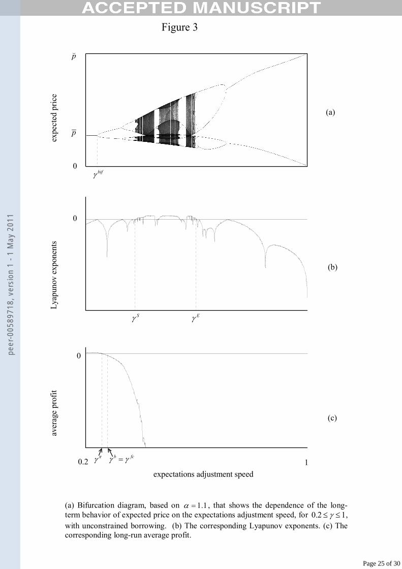
illustrates a period-three cycle, the hallmark of complex dynamics. Fig. 3(a), based on

1.1α = , shows the impact of the expectations adjustment speed, γ, on the long-term behavior

of expected price. The fixed point is stable for sufficiently slow speeds. As γ increases

through 0.24bifγ ≅ , where ( ) 1f p′ = − , a sequence of period-doubling bifurcations occurs.

For speeds between 0.381Sγ ≅ and 0.564Eγ ≅ , intervals of chaos (a positive Lyapunov

exponent in Fig. 3(b)) and of order (a negative Lyapunov exponent) are intermingled.

Increasing γ above Eγ gives rise to a sequence of period-halving (period-doubling

reversed), until a stable period-two cycle is generated at 0.712γ ≅ . As γ increases towards

1, the amplitude of the period-two cycle increases.

It should be emphasized that our model involves normal assumptions about costs and

demand and that, with the assumption of unconstrained borrowing, it constitutes a standard

cobweb model. The map f belongs to the class of difference equations analyzed by Hommes

(1994) involving adaptive expectations and non-linear but monotonic demand and supply.3

As 0fq → , the map f tends to a form similar to that analyzed by Onozaki et al. (2000), who

assume naïve expectations but cautious adjustment to the output that maximizes expected

profit. But what these studies ignore is whether the long-term behaviors implied by the

models are consistent with the long-run financial viability of producers. When this issue is

3 For this class, the difference equations are differentiable and possess a first derivative less than 1. As a

specific case, Hommes explores the properties of a map derived from an ‘S-shaped’ supply curve and a linear

demand function. His map has similar properties to our map f (it has two critical points for some 0 1γ< < and

is strictly decreasing at 1γ = ) and the qualitative properties of the dynamics are substantially identical. A

crucial difference is that, since Hommes normalizes prices by using the inflection point of his supply curve as

the new origin, his model does not permit an evaluation of profitability.

Page 8 of 30

peer

-005

8971

8, v

ersi

on 1

- 1

May

201

1

Acce

pted

Man

uscr

ipt

8

addressed, it becomes evident that there is a fundamental problem with standard cobweb

models.

For our model, as shown in Fig. 3(c), long-run average profit declines monotonically as

the speed γ increases beyond bifγ . For 0.257πγ γ> ≅ , average losses are incurred, and they

increase rapidly as γ increases towards the case of naïve expectations. Negative long-run

average profits set off alarm bells suggesting non-viability. However, the question of long-

run viability cannot be settled conclusively by examining average profits: in general,

negative average profits are neither necessary nor sufficient for financial crises to occur.

To determine whether financial crises occur, we need to consider explicitly the behaviors

of net borrowing and of financial wealth. We define bγ as the expectations adjustment speed

below which producers are always able to finance internally their desired input acquisitions

and never have recourse to borrowing. We define fcγ as the speed below which financial

crises do not occur, where, provisionally, we define a financial crisis as arising when the

representative firm’s debt is increasing period after period. Since a financial crisis can only

arise as a result of borrowing, fc bγ γ≥ . In fact, with unconstrained borrowing, financial

crises occur sooner or later (i.e., fc bγ γ= ). The latter critical speed depends inter alia on the

representative producer’s initial financial wealth. Assuming that the latter is just sufficient to

cover the cost of producing the initial expected profit maximizing output (i.e.,

( )0 0 fF q qα

= − where ( ) ( )1 1

0 0e

fq q pα

ψ−

= + ), simulations show that 0.277fc bγ γ= ≅ for the

parameters on which Fig. 3 is based. Note well that fc b πγ γ γ= > . That is, there is a range of

speeds for which, even though average profit is negative, the representative firm does not

borrow and cannot go bankrupt. In this case, the production losses are being subsidized by

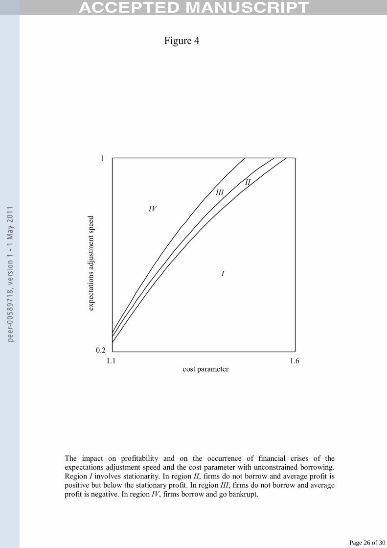
the receipt of positive net interest. Fig. 4 shows the impact on profitability and on the

Page 9 of 30

peer

-005

8971

8, v

ersi

on 1

- 1

May

201

1

Acce

pted

Man

uscr

ipt

9

occurrence of financial crises of varying both the speed γ and the cost parameter α . Region

I corresponds to parameter combinations that result in stationarity with profit π . In Region

II, average profit is positive but below the stationary profit. In Region III, average profit is

negative but firms do not borrow (and cannot go bankrupt). The boundary between Regions

III and IV shows for each α the corresponding speed bγ below which firms never borrow.

In Region IV, firms do borrow and, sooner or later, they go bankrupt. From Fig. 4, for most

parameter combinations for which the model exhibits complex behavior, firms engage in

borrowing and, with no constraints on that borrowing, they go bankrupt.

The incidence of financial crises cannot simply be eliminated by a ceteris paribus

increase in demand: increasing E (or reducing N) increases the intercept of the map f and is a

destabilizing force. With cyclical or chaotic system behavior, average profit is less than the

stationary profit, and fluctuations increase the likelihood of financial crises. Similarly,

assuming a demand curve with a constant elasticity other than 1− does not alter our

conclusions in any fundamental way.4

Before considering the nature and implications of borrowing constraints, we make two

historical observations. First, whereas the notion of negative average pure profits over the

long run may be disquieting to those brought up on the standard neoclassical theory of a

4 Extending the model to incorporate the distribution of part of the representative firm’s income to shareholders

would complicate further the relationships between average profits, borrowing and the occurrence of

bankruptcies. The greater the proportion of income that is distributed, the lower the critical speeds at and above

which borrowing and financial crises occur. With such distribution, there can be a range of speeds for which

firms borrow regularly without going bankrupt (i.e., b fcγ γ< for a given α ). Furthermore, it is possible that

the distribution of earnings may be sufficiently high that bankruptcies occur even though long-run average

profit is positive (i.e., fc πγ γ< for a given α ).

Page 10 of 30

peer

-005

8971

8, v

ersi

on 1

- 1

May

201

1

Acce

pted

Man

uscr

ipt

10

perfectly competitive industry, it would not have been troublesome to Knight. In his classic

work, Risk, Uncertainty and Profit, he advanced his strongly-held belief that “business as a

whole suffers a loss” (1971, 365): he argued that entrepreneurs, motivated by the prospect of

profits, actually realize negative pure profits on average, and they sustain this essentially

through foregoing some of the opportunity costs on those financial or physical resources that

they themselves supply to their businesses. Second, in certain respects, our challenge to

standard non-linear cobweb models echoes a largely ignored challenge to the linear cobweb

model by Buchanan in 1939. He argued that “neither perpetual fluctuation at a given

amplitude nor expanding fluctuation is theoretically possible if the supply curve is a

competitive supply curve as most writers apparently had in mind in their exposition of the

doctrine” since “losses will inevitably exceed profits” (80-81).5 He notes: “On the special

assumption that there is always a group of new producers willing to rush in and dissipate

their capitals with each swing of the cycle, the theorem may perhaps be valid” (81).

4. Constrained Borrowing

Denoting the representative producer’s financial capital fund at the beginning of period t

by tK , where this comprises both own financial wealth and the maximum that the producer

could borrow, the financial capital constraint on output is

,v t tq Kα ≤ . (17)

Maximizing expected profit subject to (17) requires

( ) ( ){ }1 1 1, min ;e

t f v t f t tq q q q p Kα αψ

−= + = + (18)

5 In contrast to our model, Buchanan’s analysis encompasses two alternative interpretations of the industry

supply curve, neither of which corresponds to the case of Ricardian increasing costs.

Page 11 of 30

peer

-005

8971

8, v

ersi

on 1

- 1

May

201

1

Acce

pted

Man

uscr

ipt

11

where ( ) ( )1 1ef tq p

αψ

−+ is the output that would maximize expected profit in the absence of a

financial constraint (see (13)) and 1/f tq K α+ is the maximum output consistent with the

financial constraint.

To accommodate the entry of a new cohort of producers to replace those that go bankrupt,

it is necessary to specify precisely when firms are deemed bankrupt and what the financial

position of entrants is. Our banks follow a simple rule: a firm is declared bankrupt if and

only if it has a financial debt that is not diminishing. That is, the representative producer is

deemed to be bankrupt at the beginning of period t iff

1 0t tF F −≤ < . (19)

We assume that where durable assets are sold to a new producer cohort, the purchase

exhausts the funds of the representative entrant so that there is no own financial capital left

for acquiring additional inputs (i.e., 0tF = for a firm entering at the beginning of period t).

The latter seems the least arbitrary assumption, and it implies at least that new firms get off

to a good start since each produces fq and receives the maximum profit in its first period.

The dynamical system is depicted in Fig. 5. The financial capital fund tK , which

necessarily depends on own financial wealth tF , may or may not depend also on the value of

the durable asset, tV . Where tK depends directly only on tF , then etp depends on 1

etp − and

on 1tF − ; and tF depends on 1etp − and on 1tF − . Given an initial expected price 0

ep and an

initial financial wealth 0F , the future time paths of etp , tK , tq , tB , tp , tπ , ty and tF are

determined uniquely; with an appropriate initial condition, the time path of tV can be

determined from that of tπ .

Page 12 of 30

peer

-005

8971

8, v

ersi

on 1

- 1

May

201

1

Acce

pted

Man

uscr

ipt

12

The system’s behavior differs from the case of unconstrained borrowing if and only if the

financial capital constraint (17) impacts on the behavior of the representative producer. Since

the constraint is never binding for parameter combinations in Regions I, II and III in Fig. 4,

the system’s dynamical behavior is necessarily the same as for the map f for unconstrained

borrowing. Therefore, the interesting ( ),γ α combinations are those in Region IV. For the

latter Region, the decomposition that occurs with unconstrained borrowing breaks down.

Since the constraint (17) shifts over time as financial wealth changes, the system’s dynamical

behavior is considerably more complicated than for unconstrained borrowing.

4.1 Pure Internal Finance

Suppose initially that producers must rely exclusively on their own financial capital. With

pure internal finance,

0t tK F= ≥ . (20)

This excludes any possibility of bankruptcy: a firm that cannot borrow never falls into debt.

Fig. 6, based on 1.1α = to permit comparisons with Fig. 3, shows the behaviors of expected

price and of long-run average profit. Comparing pure internal finance with unconstrained

borrowing for bγ γ> , the long-run behavior of expected price is not overtly very different.

Over the chaotic region, the behavior of expected price appears rather more ‘noisy’ in Fig. 6,

but the ranges of variation at any speed are similar. However, the crucial difference is not

evident from the bifurcation diagrams. Whereas recurrent financial crises are inevitable with

unconstrained borrowing for bγ γ> , bankruptcies cannot occur with pure internal finance,

notwithstanding the negative average profits. For example, for naïve expectations, the

period-two cycle with unconstrained borrowing involves a firm lifetime of just two periods;

in contrast, the period-two cycle with pure internal finance is consistent with the continuing

Page 13 of 30

peer

-005

8971

8, v

ersi

on 1

- 1

May

201

1

Acce

pted

Man

uscr

ipt

13

survival of firms. For all ( ),γ α combinations in Region IV in Fig. 4, pure internal finance

involves survival with negative average profits.

4.2 Credit Rationing

Typically, firms are able to borrow but their ability to do so is constrained. Banks, facing

the risk that a borrower may fail to repay the interest and the principal, ration credit. Lending

to producers in a wide variety of industries and facing asymmetric information, our banks

follow behavioral rules that discriminate between prospective borrowers according to their

balance sheets.6

A natural case to consider first is that where the producers’ durable asset L provides

collateral for loans. Specifically, suppose that a bank is prepared to lend a producer up to a

limit of ( )1tV r+ . Provided that the value of L does not fall, the proceeds from its sale

would cover both the principal and the interest, protecting the bank against default.7

However, in our model, this credit constraint results in the same dynamical behavior as for

pure internal finance. The explanation is that, for those parameter combinations for which

the firms’ own financial capital is insufficient to finance desired input acquisition (i.e., for

Region IV in Fig. 4), long-run average profits are negative; according to (11), the durable

asset is effectively worthless (i.e., 0tV ≅ ) and cannot be used as collateral for a loan.

A more interesting possibility is that banks discriminate between producers according to

their financial wealth levels. This would be equivalent to basing the limit on the own

6 In their macro-analysis of business cycles, Bernanke and Gertler (1989) examine the significance of the

creditworthiness of borrowers being dependent on their net worth.

7 In their analysis of credit cycles, Kiyotaki and Moore (1997, 218) invoke a similar borrowing constraint. In

their rational expectations model, agents have perfect foresight of future durable asset prices.

Page 14 of 30

peer

-005

8971

8, v

ersi

on 1

- 1

May

201

1

Acce

pted

Man

uscr

ipt

14

financial capital that producers risk in production, for example, where banks are prepared to

‘match’ the own funds invested by borrowers. Following Day (1967, 1994) and Day et al.

(1974), suppose that banks are willing to lend up to a multiple θ of a producer’s own

financial capital, where 0θ > reflects the degree of cautiousness of the banking community.8

The representative producer’s financial capital fund, including possible borrowed funds, is

then

( )1 0

0 0t t

tt

F for FK

for F

θ� + ≥= <

. (21)

Note well that, since a firm in debt cannot borrow, the simple bankruptcy rule (19),

plausible for an individual bank that lacks information about the industry, turns out to be a

sensible one for the banking community as a whole. To see this, suppose that at the outset of

period ( )1t − , the representative firm was in financial debt. Unable to borrow, it produced

fq . With each firm supplying fq to the market, each received the maximum profit π� . A

failure to make any positive contribution to paying off its debt (i.e., 1 0t tF F −≤ < ) is

equivalent to 1tr Fπ −≤� . Since the receipt of the maximum profit π� in the previous period

made no contribution to paying off the debt, the firm’s financial position is irretrievable: if it

continued in production, its debt would inexorably deteriorate period after period if

1 0t tF F −< < and would remain the same in the (fluke) case in which 1 0t tF F −= < . Thus, by

deeming firms to be bankrupt if they have made no contribution to paying off their debts,

banks are rationally cutting their losses. In contrast, if firms did make some contribution over

the previous period to paying off their debts (i.e., 1tr Fπ −>� ), it would not pay banks to

8 Fixing limits to loans is a crucial component of banks’ portfolio management. See Cohen and Hammer (1972)

and Walker (1997).

Page 15 of 30

peer

-005

8971

8, v

ersi

on 1

- 1

May

201

1

Acce

pted

Man

uscr

ipt

15

deem them to be bankrupt. Firms would continue to reduce the debts period by period until

they are cleared.9

Compared with pure internal finance (which would correspond to 0θ = ), the ability to

borrow results in much greater system volatility for bγ γ> . Fig. 7, based on 1.1α = , shows

the behaviors of expected price and of long-run average profit for 4θ = . A crude story

would be as follows. A low output in period t results both in a high price and in a high profit.

In turn, the high price results in a high expected price. Furthermore, the high profit enhances

the producers’ ability to borrow. The resulting high output in period ( )1t + gives rise to a

loss. If this loss results in the producer being in debt, output in period ( )2t + is at its

minimum level, with price and profit at their highest levels. This continues until the debt is

cleared. That the ability to borrow can result in sustained periods of debt and of low outputs

lies behind another striking feature of Fig. 7, namely, that, for 4θ = , long-run average

profits are positive. This particular increase in average profits (compared to pure internal

finance and a fortiori to the case of unlimited borrowing) is acquired without much risk to

banks, since, for 4θ = and for the assumed cost structure ( 1.1α = ), financial crises occur

only for a very few isolated speeds.

Fig. 8 shows the impact of γ and of α on borrowing, profitability and bankruptcy for

selected values of the credit rationing parameter θ . For each ( ), ,θ γ α combination, average

profits were calculated and the incidences of borrowing and bankruptcy were identified for

9 Since rπ� is the maximum conceivable value for L, our bankruptcy condition implies that a bankrupt firm’s

total wealth cannot be positive. In other words, our bankruptcy condition is equivalent to postulating that the

representative firm is deemed bankrupt if its (hypothetically) receiving the discounted present value of the

future infinite stream of the maximum possible profits would not result in a positive total wealth.

Page 16 of 30

peer

-005

8971

8, v

ersi

on 1

- 1

May

201

1

Acce

pted

Man

uscr

ipt

16

501 2000t≤ ≤ . The interpretations of the colors are shown in Table 1.10 For example, dark

green signifies that producers borrowed at least once, that long-run average profit was

negative but that no bankruptcies occurred. Note first the relationship between Fig. 8 and

Fig. 4. For ( ),γ α combinations in Regions I, II and III in Fig. 4, producers rely solely on

internal finance and cannot go bankrupt. Therefore, Regions I, II and III appear, respectively,

as white, light blue and dark blue in Fig. 8 (the level of θ being irrelevant). The borrowing

constraint only impacts ( ),γ α combinations in Region IV. As seen above, for pure internal

finance ( 0θ = ), losses are incurred for Region IV, so the latter would be dark blue. In Fig.

8(a), where banks are prepared just to match a borrower’s own funds ( 1θ = ), firms take

advantage of the opportunity to borrow, long-run average profits are negative but

bankruptcies never occur. Increasing θ can increase average profitability but at a cost of a

greater risk of financial crises. Thus, in Fig. 8(b) where 4θ = , the beneficial impact of the

higher θ is manifested in the light green areas, indicating positive average profits; the

hazards are reflected in the incidences of bankruptcies signified by the purple and red areas.

Further increases in θ increase the likelihood of financial crises. Where bankruptcies are

avoided, higher average profits are accompanied by increased variability of profits and

possibly by the representative producer being frequently in debt. For 10θ = in Fig. 8(c), the

red areas confirm the increased frequency of bankruptcies, while the yellow areas signify

that, for some ( ),γ α combinations, firms not only survive but also earn long-run average

profits above the stationary profit.11 Barely perceptible incidences of orange mean that it is

10 The colors are visible in the online version.

11 This is consistent with Huang (1995), who shows that, under certain circumstances, ‘cautious’ responses by

firms to fluctuating prices may result in long-run average profit above the stationary profit. Such responses

Page 17 of 30

peer

-005

8971

8, v

ersi

on 1

- 1

May

201

1

Acce

pted

Man

uscr

ipt

17

possible for bankruptcies to occur even though average profits exceed the stationary profit.

For yet more lax credit limits, borrowing almost invariably results in bankruptcy. As Section

3 confirmed, for unconstrained borrowing, all ( ),γ α combinations in Region 4 would be

red, signifying borrowing leading to losses and to bankruptcy.

5. Some Concluding Comments

In reality, producers are constrained in their ability to borrow. In reality, producers go

bankrupt. Our borrowing constraints and our bankruptcy condition presuppose that the

banking community follows very simple behavioral rules. Our model could be extended by

allowing credit limits to depend on the history of repayment defaults in this industry; by

assuming that the rate of interest depends on the amount borrowed; or by introducing

heterogeneity in the financial wealth levels of producers. Such amendments would surely

reinforce our central conclusion: industry performance (in terms both of profitability and of

the incidence of bankruptcies) is highly sensitive to the nature and degree of credit

restrictions.

However simple the behavioral rules of our banks, they are certainly more plausible than

the assumption (implicit in standard cobweb models) that banks are prepared to lend any

amount to a producer, even to one that is falling further and further into debt. An implication

of our model, which involves standard assumptions about costs and demand, is that

unconstrained borrowing results in bankruptcies. To put our challenge to the standard non-

linear cobweb model bluntly, a model designed to explain how prices and quantities can

involve upper bounds on the growth rates of output, which Huang suggests might be attributable to “capacity

constraints, financial constraints and cautious response to price uncertainty by firms” (261).

Page 18 of 30

peer

-005

8971

8, v

ersi

on 1

- 1

May

201

1

Acce

pted

Man

uscr

ipt

18

fluctuate endogenously is methodologically unsatisfactory if is inconsistent with the survival

of producers for precisely those parameters that result in complex dynamical behavior.

Page 19 of 30

peer

-005

8971

8, v

ersi

on 1

- 1

May

201

1

Acce

pted

Man

uscr

ipt

19

References

Bernanke, B.S., Gertler, M., 1989. Agency costs, net worth, and business fluctuations.

American Economic Review 79, 14-31.

Buchanan, N.S., 1939. A reconsideration of the cobweb theorem. Journal of Political

Economy 47, 67-81.

Cohen, K.J., Hammer, F.S., 1972. Linear programming models for optimal bank dynamic

balance sheet management. In: Szegö, G.P., Shell, K. (Eds.). Mathematical

Methods in Investment and Finance. Amsterdam: North-Holland, 387-413.

Day, R.H., 1967. A microeconomic model of business growth, decay and cycles.

Unternehmensforschung 11, 1-20.

Day, R. H., 1994. Complex Economic Dynamics. Vol. I. Cambridge: MIT Press.

Day, R. H., Morley, S., Smith, K.R., 1974. Myopic optimizing and rules of thumb in a

micro-model of industrial growth. American Economic Review 64, 11-23.

Hommes, C.H., 1994. Dynamics of the cobweb model with adaptive expectations and

nonlinear supply and demand. Journal of Economic Behavior and Organization

24, 315-335.

Huang, W., 1995. Caution implies profit. Journal of Economic Behavior and Organization.

27, 257-77.

Kiyotaki, N., Moore, J., 1997. Credit cycles. Journal of Political Economy 105, 211-248.

Knight, F. H., 1971. Risk, Uncertainty and Profit. Chicago: University of Chicago Press.

Onozaki, T., Sieg, G., Yokoo, M., 2000. Complex dynamics in a cobweb model with

adaptive production adjustment. Journal of Economic Behavior and Organization

41,101-115.

Page 20 of 30

peer

-005

8971

8, v

ersi

on 1

- 1

May

201

1

Acce

pted

Man

uscr

ipt

20

Walker, D. A., 1997. A behavioral model of bank asset management. Journal of Economic

Behavior and Organization 32, 413-431.

Page 21 of 30

peer

-005

8971

8, v

ersi

on 1

- 1

May

201

1

Acce

pted

Man

uscr

ipt

21

Borrowing Average Profit

(av.)

Bankruptcy

white � .av π= �

light blue � 0 .av π≤ < �

dark blue � . 0av < �

yellow � .av π≥ �

light green � 0 .av π≤ < �

dark green � . 0av < �

orange � .av π≥ �

purple � 0 .av π≤ < �

red � . 0av < �

Table 1

Page 22 of 30

peer

-005

8971

8, v

ersi

on 1

- 1

May

201

1

Acce

pted

Man

uscr

ipt

�

��

��������

���� ��

�� ��

�

��

����� � ��������� ���� ��� �������� ��� �������� �� ��� � ������ ��� ���� � ������

� � ����������� �������������� ����� �� ����� � ���� ����������� ��� � ���������

����� ����������! "���������

���

Page 23 of 30

peer

-005

8971

8, v

ersi

on 1

- 1

May

201

1

Acce

pted

Man

uscr

ipt

��������

�

��

�

��

�

�� �

�

�� �

��

��

��

��

��

��

�� ����������������������������������������������� ��� � ����� � � ���

�� ����������������������������������� ���� � ����� � � � ��

Page 24 of 30

peer

-005

8971

8, v

ersi

on 1

- 1

May

201

1

Acce

pted

Man

uscr

ipt

�

�

��

�

�

�����

�����

��

�� �

������

������

�� �

� �

����

��

������ ����� ���������������

��� �

������

����

��

�� ��

� �

���

���

� ��� ��

� �� ���� ���� � � � � � ���� ��� ���� � � �! �� �!�"�� �!�� ����������� ��� �!�� #���$

������! �����������������������!�������� ����� ��������������� ���� ��� ��� �

"�!�������� �������"���������%!��������������� ���������������������%!��

�����������#���$��� �� ���������

Page 25 of 30

peer

-005

8971

8, v

ersi

on 1

- 1

May

201

1

Acce

pted

Man

uscr

ipt

�

��

���

��

��� ���������� � �

���

�

� �������������� ���� �

����� ��

�� � ����� ��� ������������ ��� ��� �� � ������ �� � ��� �������� ���� �� ��� �� � � �������������� ���� ������� �������� � ����������������� �������������

���������!��! ��������������"��� �������#������������������������! �� ����������

�����! ������ ������ �����������������"��� ��������#������������������������! �� �

���������� ���! ��"��� �������#����������������������$�����

Page 26 of 30

peer

-005

8971

8, v

ersi

on 1

- 1

May

201

1

Acce

pted

Man

uscr

ipt

�

�

�� �

�

��

��� �

��� �

��� �

��

��� �

��� �

�������

����� �

�� ��� �������������������� ��������������

Page 27 of 30

peer

-005

8971

8, v

ersi

on 1

- 1

May

201

1

Acce

pted

Man

uscr

ipt

�

��

�������������

��������� ���� ������ ����

�

�������

��

�����������

�

�

���

�

������������������������������� ������ ���� � ��������������������������

Page 28 of 30

peer

-005

8971

8, v

ersi

on 1

- 1

May

201

1

Acce

pted

Man

uscr

ipt

�

��

����

�

�

������������

��� ��������

������ ����� ������������

�������

������ ����� �� � � ��� ���������� ���� ���� � ����

������ ���������������������� �������� � ����� �� � �

�

�

�

Page 29 of 30

peer

-005

8971

8, v

ersi

on 1

- 1

May

201

1

Acce

pted

Man

uscr

ipt

Figure 8ex

pect

atio

ns a

djus

tmen

t spe

ed

The impact of the expectations adjustment speed, 0.2 1γ≤ ≤ , and of the cost parameter, 1.1 1.6α≤ ≤ , on long-run profitability, borrowing and bankruptcy for different values of the credit rationing parameter θ . White signifies stationarity; light blue signifies no borrowing and a positive average profit below the stationary profit; dark blue signifies no borrowing and a negative average profit; yellow signifies borrowing (but no bankruptcies) with an average profit above the stationary profit; light green signifies borrowing (but no bankruptcies) with a positive average profit below the stationary profit; dark green signifies borrowing (but no bankruptcies) with a negative average profit; orange signifies an average profit above the stationary profit but with bankruptcies; purple signifies a positive average profit below the stationary profit but with bankruptcies; red signifies a negative average profit with bankruptcies.

(a) 1θ = (b) 4θ = (c) 10θ =

cost parameter

Page 30 of 30

peer

-005

8971

8, v

ersi

on 1

- 1

May

201

1