CURRENCY AREAS AND INTERNATIONALASSISTANCE

BY PIERRE M. PICARD AND TIM WORRALL

January 2009

This paper considers a simple stochastic model of international trade with threecountries. Two of the tree countries are in an economic union. Comparisons are madebetween equilibrium welfare for these two countries under fixed and flexible exchangerate regimes. Within the model it is shown that flexible exchange rate regimes generategreater welfare. However, we then consider comparisons of welfare when the twocountries also engage in some international assistance in order to share risk. Such risk-sharing is limited by enforcement constraints of cross border assistance. It is shown thattaking into account limited commitment risk-sharing fixed exchange rates or currencyareas can dominate flexible exchange rate regimes reversing the previous result.

KEYWORDS: Monetary union · currency areas · fiscal federalism · limitedcommitment · mutual insurance

JEL CLASSIFICATION: F12 · F15 · F31 · F33

1. INTRODUCTION

This paper contributes to the theory of optimal currency areas. In an often citedpaper Mundell (1961) argues that business cycles should be sufficiently positivelycorrelated for a common currency area to be optimal. Bayoumi (1994) formallyshows that when shocks are negatively correlated across countries a currency unionis less desirable. As a consequence, the discussion about the UK’s integration (ornon-integration) into the Euro currency area has often been driven by the fact thatUK business cycles are not well correlated with continental Europe. Equally thediscussion of when the accession countries should join the Euro currency area hasbeen dominated by the debate about the congruence of the economic cycles of theaccession countries and the rest of Europe.

One aspect of monetary integration that has received relatively little attention isthe interaction of international assistance and business cycles on the optimality ofcurrency areas. This is an important consideration since, as has been argued by Drèze

Département Economie, University of Luxembourg, 162A avenue de la Faïencerie, L-1511 Luxembourgand CORE, Université Catholique de Louvain, Louvain-la-Neuve, Belgium. E-mail: pierre.picard@uni.luand Economics, School of Social Sciences, University of Manchester, Oxford Road, Manchester, M139PL UK. E-mail: tim.worrall@manchester.ac.uk.

1

CURRENCY AREAS 2

(2000), transfers between regions can be used as a means of insurance against regionalincome shocks.1 Moreover in the case of the EU, shocks have been shown to be large(Forni and Reichlin 1999) and risk diversification incomplete (French and Poterba1991, Baxter and Jermann 1997) suggesting that there are welfare gains if moreinsurance between regions can be agreed. Although interregional transfers in the EUare currently quite small (less than 1% GDP) they do increasingly depend on regionalincome (through EU Objective 1 Funds) and further integration is likely to mean thattransfers play an increasingly prominent role is smoothing interregional fluctuations.The purpose of this paper is to address that gap and examine the interaction betweenrisk-sharing measures and the optimality of a currency union. It provides a dynamicmodel of risk-sharing in which the conclusion of Mundell is turned on its head. Acurrency union can indeed be optimal when the demand for risk sharing is high andshocks are anti-correlated.

To make the contrast with previous results sharp we model a situation wherethere are nominal wage and price rigidities. This nominal wage and price rigiditywould normally mean that there is a need for exchange rate flexibility and hencethat a monetary union is inefficient. However, we show that when the risk sharingmotivation between countries is taken into account this result may be reversed. Weshall not assume that risk sharing is perfect. Indeed we shall show that within themodel a currency union will not be optimal if risk sharing is perfect. Rather weassume that risk sharing between countries is limited by self-enforcing constraints.This is natural assumption for a currency union between sovereign states as there isno supra-national legal authority to enforce transfers. Hence countries will only makesuch transfers if they are in their own long-term interest. This long-term interestwill be determined by the future benefits of risk sharing and by the punishmentimposed for not making the requisite transfer which we assume involves a loss offuture assistance. The importance of the self-enforcement constraints is that theinefficiencies caused by nominal wage and price rigidities may increase the varianceof regional incomes in currency unions and this may make it easier to enforcetransfers as the consequences of loss of future assistance are more severe. Countriesmay thus prefer a currency union because greater transfers and insurance can besustained. That is the benefit of insurance may outweigh the inefficiency cost of afixed exchange rate and consequent real price rigidities. We shall show that this isindeed possible and that there are circumstances where a monetary union is preferredto the flexible exchange rate system because of the desire to share risk.

1 Our model is also related to the literature on fiscal federalism but in most of that literature the transfersbetween regions take place because of sharing of a public good, such as security (see also Alesina et al.1995, Persson and Tabellini 1996), rather than sharing of risk.

CURRENCY AREAS 3

Our model is stylized and designed to give an advantage to flexible exchangerates in the absence risk-sharing considerations. In this way we can show thatthe possibilities of risk sharing can be important for decisions about a currencyunion. There are many other potential factors which advantage currency unions suchas the removal of exchange rate transaction costs, the elimination of competitiveinflation and the increased stability of financial markets and so on. Qualitatively theimplications of risk sharing will be similar in these models too. What our resultsshow is that the issue of currency integration cannot be divorced from the issue offiscal integration through international assistance and that international assistance isan important factor to weigh in considering the optimality of a currency union.

For most of this paper we focus on the case where the decision to adopt a commoncurrency or not has no effect on the technology of enforcing risk sharing agreements.2

However, it is possible that a common currency will be associated with other politicaland economic aspects of integration which will improve the enforcement mechanismand thus lead to greater risk sharing.3 This will increase the desire for a currencyunion further and may also be an important benefit of a currency union itself. Ourframework also allows us to address this issue and consider when a common currencyis better if it also confers benefits in terms of the enforcement technology.

The paper is organized as it follows. Section 2 presents the model and studies theequilibria under common currency area and flexible exchange rates. In Section 3we study an economy with negatively correlated shocks and show when transfersbetween countries can be sustained and when a monetary union will deliver higherwelfare than a flexible exchange rate system. Section 4 considers extensions to thebasic model. These extensions quantitatively modify but do not qualitatively changethe main results that the common currency system sustains greater levels of transfersand may therefore lead to higher welfare for certain parameter values showing that themodel is robust at least to these generalizations. Section 5 concludes. An Appendixcontains the proofs.

2. BASIC MODEL

We consider a simple model of international trade with three countries r = H,F,W(Home, Foreign and the rest of the World). We consider that Home and Foreign haveclose economic ties or are in an economic union and shall be interested in whetherHome and Foreign should operate a currency union or retain a flexible exchangerate regime. This is the situation of the UK or accession countries and the Euro area

2 This will be made precise below.3 Historically, many countries like the U.S.A., U.K., France and others have adopted a common currency

before implementing considerable redistributive systems between their sub-national jurisdictions.

CURRENCY AREAS 4

countries or between Canada or Mexico and the US. In order to make the comparisonbetween fixed and flexible exchange rates non-trivial we shall assume that there aresome market imperfections in the labor and product markets. Following much of theliterature on currency areas we shall assume that labor is immobile across countriesand that the labor market is subject to nominal rigidities. However, we shall assumethere is free and frictionless trade between countries.4 Further we shall assume thatthe goods markets in the Home and Foreign countries is monopolistically competitivewith a continuum of varieties produced and price setting by firms. In the rest of theworld firms produce a homogenous good which we label W .

There is a unit mass of consumer-workers in country H and the same mass incountry F . In country W there is also a unit mass of consumer-workers.5 Labor issupplied inelastically in each country. We shall assume that goods are non-storableand that consumers consume both domestically-produced and foreign-producedgoods. We shall index goods by ς or ξ and let drs(ξ ) denote the demand for good ofvariety ξ from consumers in country r which is produced in country s. Similarly welet drW denote the demand for good W in country r. Individuals in all countries havethe same Dixit and Stiglitz (1977) type preference function

(1) V (Cr) = V

((∫ 1

0drr(ς)

σ−1σ dς +

∫ 1

0drs(ξ )

σ−1σ dξ

) σ µ

σ−1

d1−µ

rW

),

where V is assumed to be strictly increasing and strictly concave reflecting the factthat agents are assumed to be risk averse,6 Cr is the aggregate composite good incountry r and σ > 1 is the elasticity of substitution. The elasticity σ is a measure ofthe degree of competition between firms and the higher is σ the greater will be thedegree of competition between firms across countries. The parameter µ measuresthe relative importance of the rest of the World. If µ is close to one then the restof the World has little importance and we are left with a two country model. If µ

is small then the rest of the world is more important so there is a smaller need ofinsurance between countries H and F under flexible exchange rates. Letting prs(ς)denote the price of good ς sold in country r and produced in country s, the budget

4 Although we assume there are no transport or transactions costs to trade, these can be added to themodel without substantially changing the conclusions of the paper. Without transport costs a currencyunion is never desirable without the insurance motives we model here. Thus introducing transportationcosts will tend to strengthen our conclusions.

5 Nothing will hinge on the relative size of country W and the assumption of a unit mass for the rest ofthe world is made purely for convenience.

6 For some of the subsequent analysis and the numerical calculations we shall assume that the utilityfunction exhibits constant relative risk aversion preferences.

CURRENCY AREAS 5

constraint for the representative agent in country r is∫ 1

0drH(ς)prH(ς)dς +

∫ 1

0drF(ξ )prF(ξ )dξ + prW drW = Yr +Tr

where Yr is the income of consumers in country r and Tr is the transfer incomereceived by country r expressed in the own countries currency. As we are examiningan economic union between H and F we shall consider transfers only between theHome and Foreign country and ignore transfers with the rest of the world, that is weset TW ≡ 0. With the utility function given in (1) the demand for variety ς producedin country s from consumers in country r is

(2) drs(ς) = µprs(ς)−σ (Yr +Tr)

P1−σr

where Pr is a price index for goods produced in H and F

(3) Pr =(∫ 1

0prr(ς)1−σ dς +

∫ 1

0prs(ξ )1−σ dξ

) 11−σ

.

Likewise the demand for good W in country r is drW = (1−µ)(Yr +Tr)/prW whereprW is the price of good W in country r.

As is well-known the composite consumption is linear in income

(4) Cr = µµ(1−µ)1−µ Yr +Tr

Pµr p1−µ

rW

.

It will be convenient to emphasize the dependence of the composite consumption onthe transfer and write it as a function of the transfer received Cr(T ).

The exchange rate between currencies in the two countries H and F will dependon whether there is a single currency area or a flexible exchange rate. However,in either case, since we have assumed there is free and frictionless trade, pricessatisfy prs = εrs pss for all r 6= s, where εrs is the exchange rate that converts currencyof country s into the currency of country r. Since trade is frictionless εrs = 1/εsr.With three countries there are two independent exchange rates and we shall writeε for εHF and η for εHW . Thus εFW = ε/η . For convenience we shall also writepr(ς) for prr(ς) and pWW = pW . Therefore pHF(ς) = ε pF(ς), pFH(ξ ) = pH(ξ )/ε

and pHW = η pW . Then it is easy to check from equation (3) that PH = εPF andpFW = pHW /ε . As there are no transfers from outside H and F , TH =−εTF . In thecase of a common currency area ε = 1.

CURRENCY AREAS 6

We now consider firm behavior. Let Y = YH + εYF + ηYW denote total worldincome measured in the Home currency.7 For firms producing variety ς in country Hthe demand they face from Home and other consumers in F and W is

dH(ς) = µ

pH(ς)−σ (YH +TH)P1−σ

H+

(pF (ς)

ε

)−σ

(YF +TF)

P1−σ

F+

(pWη

)−σ

YW

P1−σ

W

= µ

pH(ς)−σ

P1−σ

HY.

Since PH = εPF and TH =−εTF demand is given by

(5) dH(ς) = µpH(ς)−σ

P1−σ

HY ; dF(ξ ) = µ

pH(ς)−σ

P1−σ

H

Yε

; dR = (1−µ)1

pW

Yη

.

Costs are determined by labor requirements which are given by a fixed coefficienttechnology where to produce one unit of output in country r requires ar units of labor.The price of labor is denoted by wr. However, we assume that the labor market isimperfect and that nominal wages are fixed and therefore normalize wr = 1.8 Withflexible exchange rates the exchange rates will adjust to achieve full employment ineach country. However, if there is a common currency between countries H and F ,the nominal rigidity in wages will cause unemployment in the relatively unproductivecountry. In Section 3 we shall assume that aH and aF are stochastic and specify asimple stochastic process. However, because input decisions will be made once ar isknown and since there are no intertemporal linkages in production or consumptionwe can determine equilibria as if ar were given. In country W , aW = 1 and we assumethat firms are perfectly competitive. Thus we normalize so that pW = 1 which inturn implies pHW = η and pFW = η/ε . In countries H and F firms are assumed tobe monopolistically competitive and will set prices to maximize profits given wagecosts and demand functions. Given the fixed coefficients and the iso-elastic demandfunctions given in equation (2), prices are set at a mark-up over cost

(6) pr(ς) =σ

σ −1ar, r ∈ {H,F}.

7 Note that transfers do not affect world demand.8 Assuming that nominal wages are completely inflexible is obviously an extreme assumption which

we make for convenience only. As argued by Mundell (1961) this a priori makes a currency union lessdesirable.

CURRENCY AREAS 7

It follows from equation (6) that all firms in countries H and F set the same pricewhich is simply a mark-up over costs. This mark-up depends on the elasticity ofsubstitution between commodities. As suggested above the elasticity of substitutionis a measure of competition. When substitution is perfect (σ = ∞) there is perfectcompetition and price equal marginal cost. When σ is close to one mark-ups becomelarge. It also follows from equation (6) that demand is the same for all varietiesdr(ς) = dr in a given country. Thus total labor demand is simply `r = ardr. Byassumption all profits accrue to firms’ owners and for convenience we assume that allprofits are spent locally. Thus the national income in country r is Yr = prdr = pr`r/ar.Using equation (6) national income is

(7) YH =σ

σ −1`H and YF =

σ

σ −1`F .

Since pW = 1, `W = 1 and aW = 1, national income in W is YW = 1. Equally theprice index of equation (3) can be re-written using equation (6) as

PH =(

p1−σ

H + ε1−σ p1−σ

F) 1

1−σ =σ

σ −1(a1−σ

H + ε1−σ a1−σ

F) 1

1−σ = εPF .

An equilibrium is then a set of prices and demands such that (i) consumers maxi-mize their utility given their budget constraint and given prices, (ii) firms set theirprofit maximizing prices and (iii) product markets clear. Since the labor market is im-perfect in countries H and F we do not assume that the labor market clears and theremay be some situations, discussed below, where there is unemployment. Whetherlabor markets clear or not, the product demand equal product supply conditions arederived from equations (5) and the fixed coefficient technology as

(8) µpH(i)−σY

P1−σ

H=

`H

aHand µ

pF(i)−σ(Y

ε

)P1−σ

F=

`F

aF

together with the rest of the World condition η = (1− µ)Y . Using the fact thatPH = εPF and pH/pF = aH/aF and taking the ratio of the two equations in (8) givesexpressions for the two exchange rates

(9) ε =(

aH

aF

) σ−1σ(

`H

`F

) 1σ

and η =σ(1−µ)(σ −1)µ

(`H + ε`F) .

CURRENCY AREAS 8

These conditions will determine either the exchange rates ε and η or if ε is fixed thefirst condition determines level of employment in either country H or F . Note thatbecause all product markets clear, Walras’s law implies that trade is also balanced.

2.1. Common currency area

We now consider the equilibrium in which countries H and F form a commoncurrency area so that ε = 1. In this case the price index is the same in both countries,PH = PF . Letting P denote this common index,

(10) P =(

p1−σ

H + p1−σ

F) 1

1−σ =σ

σ −1(a1−σ

H +a1−σ

F) 1

1−σ .

There are two cases to consider depending on the sign of aH − aF . If aH < aF

the Home country is relatively more productive and requires less labor to produceany given quantity of output. With this parametrization and fixed wages it is easyto check that a share of country F’s labor force will be unemployed, `F < 1, asits costs will be higher and hence demand will be lower. In contrast there will befull employment, `H = 1, in country H. It therefore follows from equation (9) that`F = (aH/aF)σ−1 < 1. If on the other hand aH > aF then there will be unemploymentin the Home country and `H = (aH/aF)1−σ < 1 = `F . Using equation (4) and theprice index P given by equation (10), the composite consumption in each of the twocountries is

Ccr (T ) = µ

(`r +

(σ −1

σ

)T)

(`H + `F)(µ−1) (a1−σ

H +a1−σ

F) µ

σ−1

where r = H,F and where the superscript c denotes that the consumption is undera currency union. Hence the level of employment in the two countries is given as`H = min

{(aH/aF)1−σ ,1

}and `F = min

{(aH/aF)σ−1 ,1

}.

2.2. Flexible exchange rate system

We now consider equilibrium output and consumption under a flexible exchangerate regime. The introduction of an exchange rate provides an additional instrumentto allow relative prices to alter and production and employment to increase. Althoughnominal wages are fixed at wH = wF = 1 the exchange rate allows the relative wagesεwF/wH to adapt. Under a flexible exchange rate regime there is no real wagerigidity so that labor markets clear in both the high and low productivity countries,i.e. `H = `F = 1. Then equilibrium output in both H and F is YH = YF = σ/(σ −1)

CURRENCY AREAS 9

and the two exchange rates are determined from (9):

(11) ε =(

aH

aF

) σ−1σ

and η =σ(1−µ)(σ −1)µ

(1+ ε).

If aH < aF then country F has relatively low productivity and its currency depreciatesmaking its exports relatively cheaper to the Home country. Likewise if aH > aF thencountry F is relatively more productive and its currency will appreciate so that itsexports become relatively more expensive to the Home country. With this exchangerate adjustment and remembering that PH = εPF , the composite consumption in theHome country is given from equation (4) as

C fH(T ) = µ

(1+(

σ −1σ

)T)

(1+ ε)(µ−1) (a1−σ

H + ε1−σ a1−σ

F) µ

σ−1

where the superscript f indicates that the consumption is calculated under flexibleexchange rates and where the exchange rate ε is as given in equation (11). LikewiseC f

F(T ) = εC fH(T ).

2.3. Risk and risk sharing

Shocks to productivity will change prices and hence consumptions. A domesticproductivity improvement say, leads to a fall in the prices of domestics productsand, since the elasticity of substitution is greater than one, a more than proportionateshift of consumers’ demand toward those products. Domestic sales and exportsincrease whereas foreign sales and exports falls. With a fixed exchange rate domesticconsumption increases relative to foreign consumption. In a flexible exchange rateregime, the domestic currency appreciates but does not fully compensate the foreigncountry for its relative loss of competitiveness. Foreign consumers and workersare still relatively worse off. Thus shocks to productivity produce fluctuations incountries’ wealth and create a desire for risk sharing even in the case of a flexibleexchange rate regime.9 In the next section we shall examine a special case whereproductivity shocks are negatively correlated and hence there will be a strong desirefor risk sharing.

Before examining risk sharing we consider the benchmark case where there notransfers between countries. In the absence of transfers, an appropriate exchange ratepolicy is one that achieves the highest aggregate consumption. One readily showsthat C f

r (0)≥Ccr (0) for r = H,F . Thus we have the standard result

9 If preferences were Cobb-Douglas (corresponding to σ = 1) then the terms of trade fully absorb theeffect of the productivity shocks and there is no need for inter-regional risk sharing.

CURRENCY AREAS 10

PROPOSITION 1: In the absence of any transfers (Tr = 0), aggregate consumptionat any state is higher under flexible exchange rate system: C f

r (0)≥Ccr (0), r = H,F.

Proposition 1 shows that if there are no transfers between countries H and F then acommon currency area will always be dominated by a flexible exchange rate regime.Thus if in our model a common currency is desirable it derives from the risk-sharingmotive.

3. CURRENCY AREAS UNDER NEGATIVELY CORRELATED SHOCKS

We shall now consider transfers between countries H and F and how this affectsthe result that a flexible exchange rate regime dominates a common currency area thatwe have seen in Proposition 1. To do this we will need to specify a stochastic processfor productivity shocks so that there are some potential mutual gains to transfers. Therole of shocks has often played a key role in debates about common currency areas.Taking into account transactions costs Mundell (1961) argues that business cyclesshould be sufficiently positively correlated for a common currency area to be optimal.Bayoumi (1994) formally shows that negative correlation of shocks makes currencyunions less desirable. As a consequence, the discussion about the UK’s integrationor non-integration in the Euro currency area has often been driven by the fact thatUK business cycles are not well correlated with continental Europe.

In this section we shall show that the conclusion of Mundell (1961) can be reversedwhen self-enforcing transfers are taken into account. That is it is shown that a com-mon currency area can be optimal when shocks are negatively correlated. To do thiswe take the extreme assumption that shocks are perfectly negatively correlated. Thuswe will make assumptions, absence of transactions costs and negatively correlatedshocks, that are usually seen as inimical to currency unions, yet show that a commoncurrency area can be optimal in these circumstances. Our argument lies in the factthat when there are productivity shocks and income variability across countries it willbe desirable to try and smooth these shocks by making transfers between countries.However, transfers across countries may be difficult to legally enforce and thereforesuch insurance transfers must be self-enforcing and enforcement may sometimes behelped by the threat of a more severe punishment.

To proceed we shall assume that the technology in countries H and F is stochastic.We shall assume there are just two symmetric states, so that the two countrieseither have a good or a bad productivity shock. Further we suppose that thesestates are perfectly negatively correlated states so that the labor requirements are(aH ,aF) = (z,1) in state 1 and (aH ,aF) = (1,z) in state 2. We assume that z < 1so that the Home country has a good productivity shock is state 1 and the Foreign

CURRENCY AREAS 11

country has the good productivity shock in state 2. To preserve symmetry we assumethat each state occurs with equal probability. With these assumptions, the aggregatecomposite consumption under the common currency in the two states is given by

CcG(T ) = µ

(1+(

σ −1σ

)T)

z(µ−1)(σ−1) (1+ z1−σ) σ(µ−1)+1

σ−1

CcB(T ) = µ

(zσ−1 +

(σ −1

σ

)T)

z(µ−1)(σ−1) (1+ z1−σ) σ(µ−1)+1

σ−1

where CcG(T ) is the consumption of the Home (Foreign) country in state 1 (2) when

it experiences a good productivity shock and CcB(T ) is the consumption of the Home

(Foreign) country in state 2 (1) when it experiences a bad productivity shock. Thetransfer T is the amount received and expressed in the countries own currency. Sincezσ−1 < 1 it can be seen that absent any transfers the Home (Foreign) country hashigher consumption in state 1 (2), when it experiences a positive productivity shock.

Under the flexible exchange rate regime the exchange rate in is ε1 = zσ−1

σ < 1 instate 1 as the Foreign currency depreciates when the Home country has a positiveproductivity shock. In contrast, in state 2 when the Foreign country has a positiveproductivity shock its exchange rate appreciates to ε2 = z

1−σσ > 1. Then calculating

the aggregate composite consumption in each state gives

C fG(T ) = µ

(1+(

σ −1σ

)T)

z1−σ

σ

(1+ z

1−σσ

) σ(µ−1)+1σ−1

and C fB(T ) = z

σ−1σ C f

G(T ). As zσ−1

σ < 1 it can be seen that absent any transfers theHome (Foreign) country has higher consumption in state 1 (2) when it has positiveproductivity shock than in state 2 (1), i.e. C f

G(0) > C fB(0).

3.1. First-best transfers

In this section we determine the first-best transfers and show that if the first-besttransfers are implemented, then the flexible exchange rate regime yields greaterwelfare. The first-best transfers will equalize composite consumptions whethercountries have good or bad productivity shocks. Let τ i

∗ denote the transfer receivedby the country with the bad productivity shock under regime i ∈ {c, f}. This will bethe transfer received by the Home (Foreign) country in state 2 (1).

With a common currency the transfer received by the country with the bad produc-tivity shock equals the transfer made by the country with the good productivity shock.Thus the first-best transfer can be found by solving Cc

G(−τ) = CcB(τ). Calculating

CURRENCY AREAS 12

this transfer and the first-best composite consumption Cc∗

τc∗ =

12

σ

σ −1(1− zσ−1) and Cc

∗ =12

µzµ(σ−1) (1+ z1−σ) µσ

σ−1 .

As zσ−1 < 1, the transfer τc∗ is positive and decreasing in z (a larger value of z is

a smaller shock). Therefore in this simple model transfers are independent of therest of the World. This is for two reasons. First, the transfer has no effect on worldincome Y and secondly the effect of the degree of preference for rest of the Worldgoods, µ is symmetric across states.

Under flexible exchange rates if τf∗ is received by the country with the bad pro-

ductivity shock then the transfer made by the country with the good productivityshock is z

σ−1σ τ

f∗ . In state 1 (2) it is the Home (Foreign) country which has the good

productivity shock so the transfer made is ε1τf∗ (τ f

∗ /ε2) where ε1 = zσ−1

σ = 1/ε2.The first-best transfer is therefore found by solving C f

G(−zσ−1

σ τf∗ ) = C f

B(τ f∗ ). This

gives the first-best transfer and consumption

τf∗ =

12

σ

σ −1

(z

1−σσ −1

)and C f

∗ =12

µ

(1+ z

1−σσ

) µσ

σ−1.

Since z1−σ

σ > 1, the transfer is positive and decreasing in z. Again this transfer doesnot affect Y and is independent of µ .

It is natural to expect that lower consumption with no transfers implies lowerconsumption under full insurance and this is demonstrated in the next proposition.

PROPOSITION 2: First best transfers yield higher aggregate utility under flexibleexchange rate system: C f

∗ ≥Cc∗.

Proposition 2 shows that if it were possible to sustain the first-best transfers thenthe common currency area would be sub-optimal. Thus we know from Propositions 1and 2 that if either first-best transfers or no transfers are sustainable then the flexibleexchange rate dominates. This should not be a surprise. We have deliberately set upthe model to give advantages to the flexible exchange rate regime. We shall however,be interested in cases where the common currency regime sustains more insurancethan the flexible exchange rate regime. Before doing so it will be useful to considerparameter values for which the common currency regime with first-best transfersmay dominate the flexible exchange rate regime with no transfers.

The common currency regime with first-best transfers generates utility V (Cc∗).

The flexible exchange rate regime with no transfers generates expected utility

CURRENCY AREAS 13

E[V (C f (0))] = (1/2)V (C fB(0)) + (1/2)V (C f

G(0)). The common currency regimewith first-best transfers will dominate when agents are highly risk averse and whenthe uncertainty is high; in this case, the agents strongly favor the constant consump-tion in the common currency area. Highly risk averse agents will prefer the regimeyielding the highest level of the worst consumption Cc

∗ or C fB(0). When z tends

to zero so that shocks are very large, the ratio Cc∗/C f

B(0) tends to infinity, whichmakes the common currency area a better alternative. Equally the ratio Cc

∗/C fB(0)

tends to 1 from above if and only if σ < 1/µ . Thus low values of the elasticityof substitution and large risk aversion a common currency will be better even forsmall shocks. Conversely if the elasticity of substitution is large (σ > 1/µ), which isalways the case if µ = 1, then the flexible exchange rate regime always dominatesfor sufficiently small shocks no matter what the degree of risk aversion. This will bemore generally true if agents are not too risk averse and shocks are small. Then it isto be expected that the flexible exchange rate regime with no transfers will dominate;agents accept the risk of a fluctuating consumption for the benefit of price flexibility.To further examine this interaction between the degree of risk aversion and the degreeof uncertainty in more detail we will use the utility function exhibiting a constantcoefficient of relative risk aversion (CRRA)

V (C) =

{C1−γ

1−γif γ > 0 and γ 6= 1

ln(C) if γ = 1

where γ is the coefficient of relative risk aversion.10

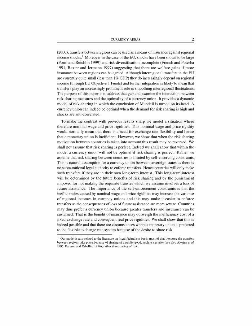
PROPOSITION 3: For any level of constant relative risk aversion γ , there exist athreshold z ∈ (0,1) such that (i) the common currency regime with first-best transfersdominates the flexible exchange rate regime with no transfers if z < z (shocks arelarge) and (ii) the latter dominates the former if z > z (shocks are small).

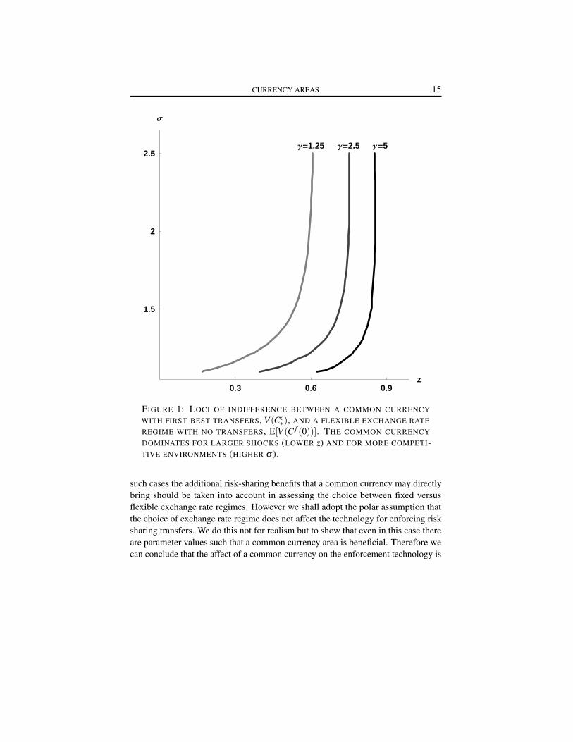
Figure 1 provides an illustration of the proposition showing how z varies with σ

and γ . The locus of indifference between the common currency regime with first-besttransfers and the flexible exchange rate regime with no transfers is drawn for threedifferent values of the coefficient of relative risk aversion γ .11 To the left of each linez < z so that V (Cc

∗) > E[V (C f (0))] and the common currency regime with first-besttransfer dominates the flexible exchange rate regime with no transfers. We see that for

10 We use the constant relative risk aversion function below for our numerical calculations but none of theresults hinge on this assumption.11 The figure is drawn for µ = 0.05. Larger values of µ slightly shifts the curves to the left withoutqualitatively affecting the result.

CURRENCY AREAS 14

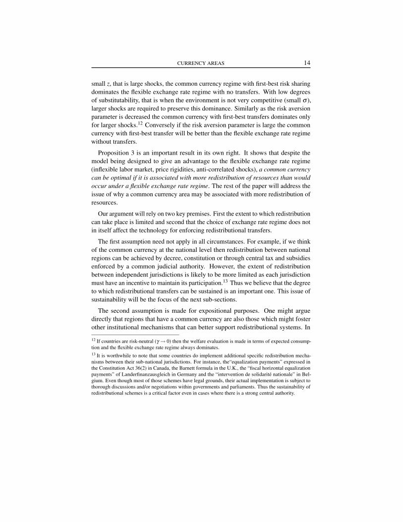
small z, that is large shocks, the common currency regime with first-best risk sharingdominates the flexible exchange rate regime with no transfers. With low degreesof substitutability, that is when the environment is not very competitive (small σ ),larger shocks are required to preserve this dominance. Similarly as the risk aversionparameter is decreased the common currency with first-best transfers dominates onlyfor larger shocks.12 Conversely if the risk aversion parameter is large the commoncurrency with first-best transfer will be better than the flexible exchange rate regimewithout transfers.

Proposition 3 is an important result in its own right. It shows that despite themodel being designed to give an advantage to the flexible exchange rate regime(inflexible labor market, price rigidities, anti-correlated shocks), a common currencycan be optimal if it is associated with more redistribution of resources than wouldoccur under a flexible exchange rate regime. The rest of the paper will address theissue of why a common currency area may be associated with more redistribution ofresources.

Our argument will rely on two key premises. First the extent to which redistributioncan take place is limited and second that the choice of exchange rate regime does notin itself affect the technology for enforcing redistributional transfers.

The first assumption need not apply in all circumstances. For example, if we thinkof the common currency at the national level then redistribution between nationalregions can be achieved by decree, constitution or through central tax and subsidiesenforced by a common judicial authority. However, the extent of redistributionbetween independent jurisdictions is likely to be more limited as each jurisdictionmust have an incentive to maintain its participation.13 Thus we believe that the degreeto which redistributional transfers can be sustained is an important one. This issue ofsustainability will be the focus of the next sub-sections.

The second assumption is made for expositional purposes. One might arguedirectly that regions that have a common currency are also those which might fosterother institutional mechanisms that can better support redistributional systems. In

12 If countries are risk-neutral (γ → 0) then the welfare evaluation is made in terms of expected consump-tion and the flexible exchange rate regime always dominates.13 It is worthwhile to note that some countries do implement additional specific redistribution mecha-nisms between their sub-national jurisdictions. For instance, the“equalization payments” expressed inthe Constitution Act 36(2) in Canada, the Barnett formula in the U.K., the “fiscal horizontal equalizationpayments” of Landerfinanzausgleich in Germany and the “intervention de solidarité nationale” in Bel-gium. Even though most of those schemes have legal grounds, their actual implementation is subject tothorough discussions and/or negotiations within governments and parliaments. Thus the sustainability ofredistributional schemes is a critical factor even in cases where there is a strong central authority.

CURRENCY AREAS 15

0.3 0.6 0.9z

1.5

2

2.5

Σ

Γ=1.25 Γ=2.5 Γ=5

FIGURE 1: LOCI OF INDIFFERENCE BETWEEN A COMMON CURRENCYWITH FIRST-BEST TRANSFERS, V (Cc

∗), AND A FLEXIBLE EXCHANGE RATEREGIME WITH NO TRANSFERS, E[V (C f (0))]. THE COMMON CURRENCYDOMINATES FOR LARGER SHOCKS (LOWER z) AND FOR MORE COMPETI-TIVE ENVIRONMENTS (HIGHER σ ).

such cases the additional risk-sharing benefits that a common currency may directlybring should be taken into account in assessing the choice between fixed versusflexible exchange rate regimes. However we shall adopt the polar assumption thatthe choice of exchange rate regime does not affect the technology for enforcing risksharing transfers. We do this not for realism but to show that even in this case thereare parameter values such that a common currency area is beneficial. Therefore wecan conclude that the affect of a common currency on the enforcement technology is

CURRENCY AREAS 16

not a necessary pre-condition for the optimality of a common currency area whencountries share risk.

3.2. Sustainable Assistance

As we know that the flexible exchange rate regime dominates if the first-besttransfers can be enforced we shall consider situations where first-best transfer cannotbe achieved. There may be many reasons for this. We shall consider the casewhere the first-best transfers cannot be achieved because there is no supra-legalauthority to enforce transfer across countries. To allow for the possibility of transferswhen commitment is limited we assume that countries interact repeatedly over aninfinite horizon. Since transfers cannot be legally enforced, countries can renege onany agreement if they find it in their interest not to make a transfer and hence anyassistance programme has to be designed to be self-enforcing. Thomas and Worrall(1988) examine self-enforcing wage contracts between an employer an an employeeand a similar approach can be applied here. Thus we presume that countries make atacit agreement on a programme of mutual assistance and specify a state contingenttransfer to be made by the country with the good productivity shock which is receivedby the country with the bad productivity shock. We shall assume that any breach ofthis tacit agreement results in a breakdown in which no transfers are made.14,15

To consider such self-enforcing transfers between countries H and F let ht denotethe history of good and bad outcomes for a particular country.16 Let Gt denote thegood productivity shock outcome at date t and Bt denote bad productivity shockoutcome at date t. Then ht is a list of G’s and B’s where h0 = /0. An assistanceprogramme in regime i ∈ {c, f} then specifies a transfer τ i

B(ht−1) to made to thecountry with the bad productivity shock if the previous history is ht−1 and thetransfer to be made by the country with the good productivity shock τ i

G(ht−1). Theshort-term loss to the country with a good productivity shock of making the requiredtransfer at time t ≥ 1 relative to making no transfer is V (Ci

G(−τ iG(ht−1)))−V (Ci

G(0)).

14 A breakdown in which no transfers are made is the worst possible outcome and is sub-game perfect.It is not however renegotiation-proof. Nevertheless it can be shown that in the current context replacingthese punishments with one that are renegotiation-proof will not change the qualitative or quantitativeproperties of the assistance programme.15 There are other possible assumptions one could make about behavior in the breakdown. For example astricter punishment could be imposed whereby there is reversion to trade autarky. Alternatively a weakerpunishment would be to assume that following any breakdown in the insurance arrangements there wouldbe a total breakdown of the currency union itself and a return to a flexible exchange rate regime withouttransfers.16 As we have assumed that shocks are perfectly negatively correlated this history has only to be specifiedfor one arbitrary country and is equivalent to specifying a history of states. We are also assuming that allother aspects of the economy are unchanging over time.

CURRENCY AREAS 17

Likewise the short-term gain at date t ≥ 1 for the country receiving a transfer isV (Ci

B(τ iB(ht−1)))−V (Ci

B(0)). To evaluate future gains and losses we shall assumethat countries discount the future by a common discount factor δ ∈ (0,1). Then thediscounted long-term gain from adhering to the agreed transfers from the next periodis (discounted back to period t +1)

E[ ∞

∑j=0

δj ( 1

2

[V (Ci

G(−τiG(ht+ j)))−V (Ci

G(0))]+ 1

2

[V (Ci

B(τ iB(ht+ j)))−V (Ci

B(0))])]

where the expectation E is taken over all future histories of good and bad productivityshocks from date t onward, τ i

G(ht+ j) is the transfer promised to be made by thecountry with the good productivity shock at date t + j +1 given that the history up totime t was ht and τ i

B(ht+ j) is the transfer to be received by the country with the badproductivity shock at date t + j +1 given that the history up to time t was ht . LettingV i

G(ht) denote the net discounted net utility from date t +1 for the country with thegood productivity shock, i.e. where the history is ht+1 = (ht ,Gt+1), and V i

B(ht) bethe net utility for a country with a bad productivity shock, i.e. where the history isht+1 = (ht ,Bt+1), we have the recursive equations

V iG(ht) = V (Ci

G(−τiG(ht−1)))−V (Ci

G(0))+δ[ 1

2V iG(ht ,Gt+1)+ 1

2V iB(ht ,Bt+1)

],

V iB(ht) = V (Ci

B(τ iB(ht+ j)))−V (Ci

B(0))+δ[ 1

2V iG(ht ,Gt+1)+ 1

2V iB(ht ,Bt+1)

].

A country will make a transfer if the expected discounted risk-sharing benefits fromfuture transfers exceed the costs of making the current transfer. Since reneging leadsto exclusion, the discounted net utilities must be non-negative at every history

(12) V iG(ht)≥ 0 and V i

B(ht)≥ 0 ∀ ht .

We shall say that an assistance programme is sustainable if (12) is satisfied. Inaddition we shall say that the assistance programme is feasible if τc

G(ht) = τcB(ht)

for all ht under the common currency regime or τf

G(ht) = zσ−1

σ τf

B(ht) under flexibleexchange rates.

We next compare the welfare and establish the sustainability conditions for eachof the two different exchange rate regimes.

3.3. Sustainable first best

In this subsection we consider the discount factors for which the first best-besttransfers are sustainable. The first-best transfers are history independent and provideconsumption of Ci

∗ in both countries. Because the first-best transfers are independent

CURRENCY AREAS 18

of history and because a country will only breach when it has a good productivityshock and is called upon to make a transfer, they are sustainable if and only if

V (Ci∗)−V (Ci

G(0))+ δ

(1−δ )

{ 12

[V (Ci

∗)−V (CiG(0))

]+ 1

2

[V (Ci

∗)−V (CiB(0))

]}≥ 0.

Rewriting this equation shows that these transfers are sustainable for discount factorsabove a critical level δ

iwhere

δi ≡

V (CiG(0))−V (Ci

∗)12

[V (Ci

G(0))−V (CiB(0))

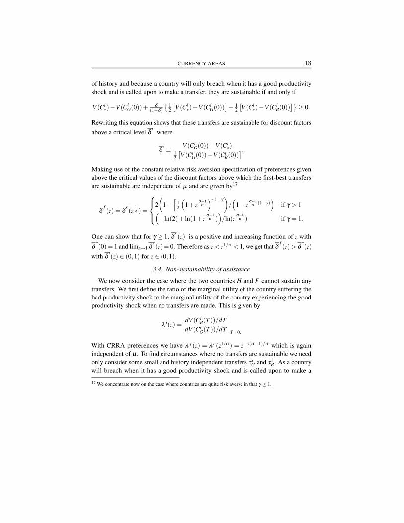
] .Making use of the constant relative risk aversion specification of preferences givenabove the critical values of the discount factors above which the first-best transfersare sustainable are independent of µ and are given by17

δf(z) = δ

c(z

1σ ) =

2(

1−[

12

(1+ z

σ−1σ

)]1−γ)

/(

1− zσ−1

σ(1−γ)

)if γ > 1(

− ln(2)+ ln(1+ zσ−1

σ ))/ln(z

σ−1σ ) if γ = 1.

One can show that for γ ≥ 1, δc(z) is a positive and increasing function of z with

δc(0) = 1 and limz→1 δ

c(z) = 0. Therefore as z < z1/σ < 1, we get that δ

f(z) > δ

c(z)

with δi(z) ∈ (0,1) for z ∈ (0,1).

3.4. Non-sustainability of assistance

We now consider the case where the two countries H and F cannot sustain anytransfers. We first define the ratio of the marginal utility of the country suffering thebad productivity shock to the marginal utility of the country experiencing the goodproductivity shock when no transfers are made. This is given by

λi(z) =

dV (CiB(T ))/dT

dV (CiG(T ))/dT

∣∣∣∣T=0.

With CRRA preferences we have λ f (z) = λ c(z1/σ ) = z−γ(σ−1)/σ which is againindependent of µ . To find circumstances where no transfers are sustainable we needonly consider some small and history independent transfers τ i

G and τ iB. As a country

will breach when it has a good productivity shock and is called upon to make a

17 We concentrate now on the case where countries are quite risk averse in that γ ≥ 1.

CURRENCY AREAS 19

transfer, no transfer is sustainable if

V (CiG(−τ

iG))−V (Ci

G(0))

+ δ

(1−δ )

{ 12

[V (Ci

G(−τiG))−V (Ci

G(0))]+ 1

2

[V (Ci

B(τ iB))−V (Ci

B(0))]}

< 0.(13)

Approximating the left hand side around no transfers (τ iB = τ i

G = 0) gives the con-dition (1− (δ/2))+(δ/2)λ i(z) < 0. This gives a critical discount factor δ

i belowwhich no transfers can be sustained in regime i∈ {c, f}. Using the assumption of con-stant relative risk aversion preferences gives δ

f = δc(z1/σ ) = 2/

(1+ z−γ(σ−1)/σ

).

One readily can show that δc(z) is a positive and increasing function of z with

limz→0 δc(z) = 0 and δ

c(1) = 1. Therefore δc(z) < δ

f (z). This together with thecondition of the previous subsection gives the following result.

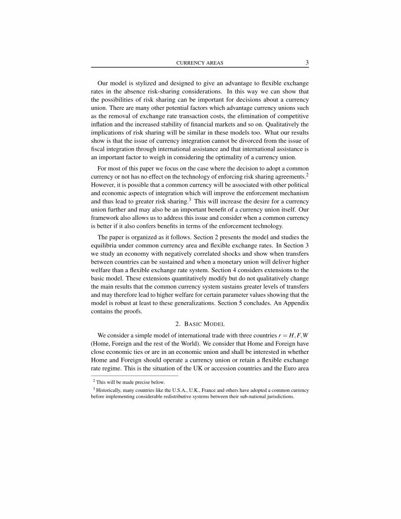
PROPOSITION 4: Common currency areas are more likely to sustain an equi-librium with first best transfers and less likely to sustain an equilibrium with zerotransfers than flexible exchange rate systems.

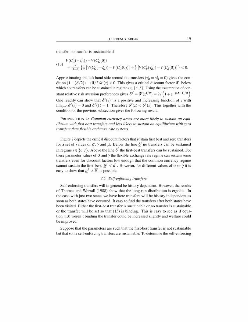
Figure 2 depicts the critical discount factors that sustain first best and zero transfersfor a set of values of σ , γ and µ . Below the line δ

i no transfers can be sustainedin regime i ∈ {c, f}. Above the line δ

ithe first-best transfers can be sustained. For

these parameter values of σ and γ the flexible exchange rate regime can sustain sometransfers even for discount factors low enough that the common currency regimecannot sustain the first-best, δ

f < δc. However, for different values of σ or γ it is

easy to show that δf > δ

cis possible.

3.5. Self-enforcing transfers

Self-enforcing transfers will in general be history dependent. However, the resultsof Thomas and Worrall (1988) show that the long-run distribution is ergodic. Inthe case with just two states we have here transfers will be history independent assoon as both states have occurred. It easy to find the transfers after both states havebeen visited. Either the first-best transfer is sustainable or no transfer is sustainableor the transfer will be set so that (13) is binding. This is easy to see as if equa-tion (13) weren’t binding the transfer could be increased slightly and welfare couldbe improved.

Suppose that the parameters are such that the first-best transfer is not sustainablebut that some self-enforcing transfers are sustainable. To determine the self-enforcing

CURRENCY AREAS 20

0.1 0.3 0.5 0.7z

0.3

0.6

0.9

∆

∆��c

∆��f

∆��c∆

��f

FIGURE 2: MAXIMUM AND MINIMUM DISCOUNT FACTORS WHICH SUSTAINNO TRANSFERS OR FIRST-BEST TRANSFERS: γ = 2, µ = 0.05 AND σ = 1.5.

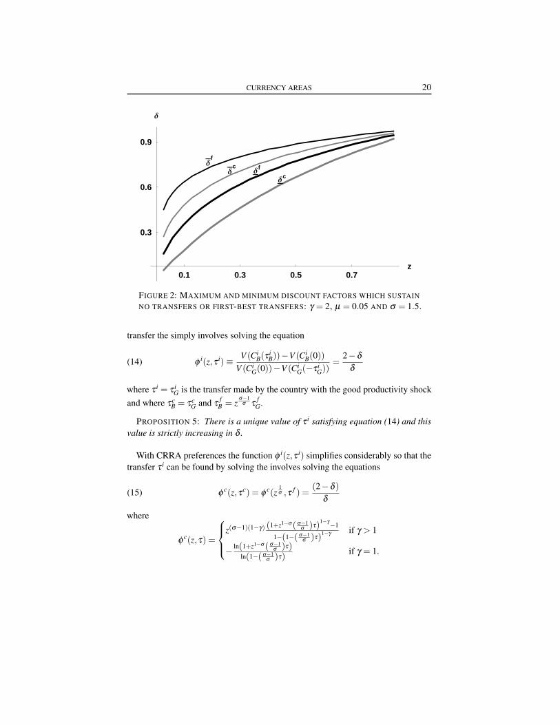
transfer the simply involves solving the equation

(14) φi(z,τ i)≡ V (Ci

B(τ iB))−V (Ci

B(0))V (Ci

G(0))−V (CiG(−τ i

G))=

2−δ

δ

where τ i = τ iG is the transfer made by the country with the good productivity shock

and where τcB = τc

G and τf

B = zσ−1

σ τf

G.

PROPOSITION 5: There is a unique value of τ i satisfying equation (14) and thisvalue is strictly increasing in δ .

With CRRA preferences the function φ i(z,τ i) simplifies considerably so that thetransfer τ i can be found by solving the involves solving the equations

(15) φc(z,τc) = φ

c(z1σ ,τ f ) =

(2−δ )δ

where

φc(z,τ) =

z(σ−1)(1−γ) (1+z1−σ( σ−1

σ )τ)1−γ−1

1−(1−( σ−1σ )τ)1−γ if γ > 1

− ln(1+z1−σ( σ−1σ )τ)

ln(1−( σ−1σ )τ) if γ = 1.

CURRENCY AREAS 21

With this specification it is clear that since z1/σ < z we have that τ f < τc so thata greater transfer can be sustained under a currency union that under a flexibleexchange rate. In addition it is possible to show that φ i(z,τ i) is strictly decreasing inz. Thus a larger shock (smaller value of z) will mean that a larger transfer τ i can besustained.

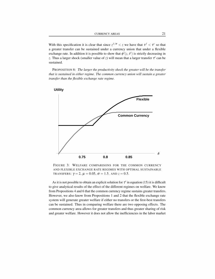
PROPOSITION 6: The larger the productivity shock the greater will be the transferthat is sustained in either regime. The common currency union will sustain a greatertransfer than the flexible exchange rate regime.

0.75 0.8 0.85∆

Utility

Common Currency

Flexible

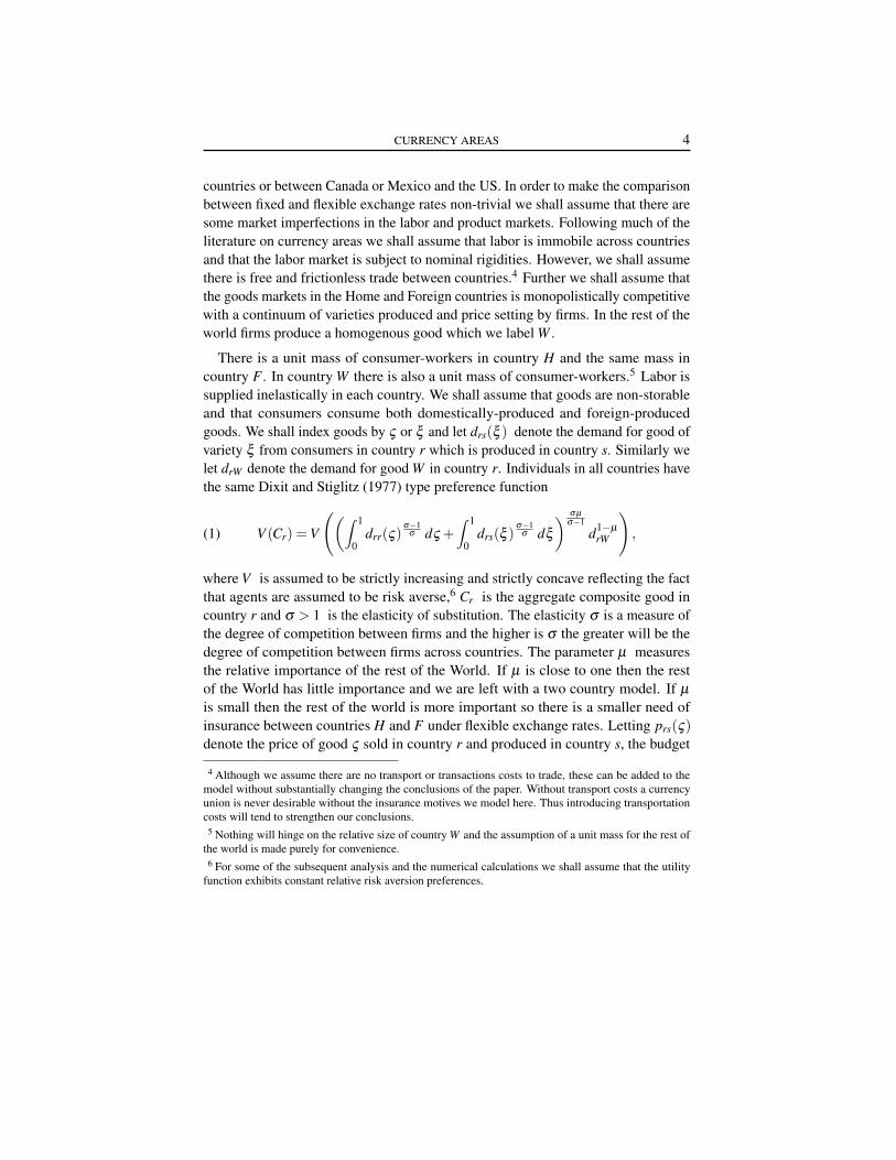
FIGURE 3: WELFARE COMPARISONS FOR THE COMMON CURRENCYAND FLEXIBLE EXCHANGE RATE REGIMES WITH OPTIMAL SUSTAINABLETRANSFERS: γ = 2, µ = 0.05, σ = 1.5. AND z = 0.5.

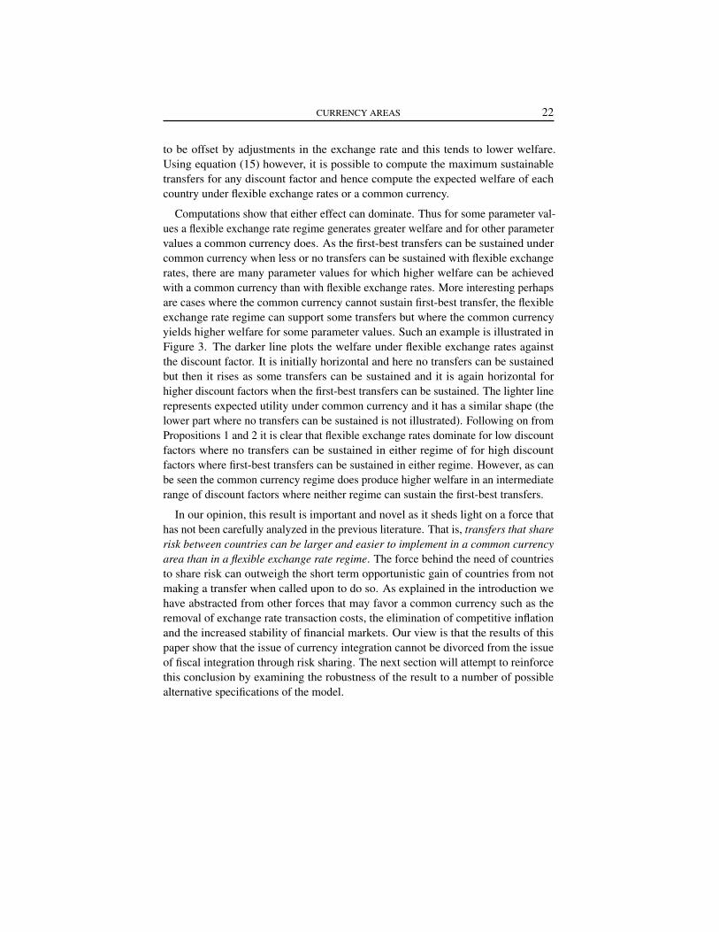
As it is not possible to obtain an explicit solution for τ i in equation (15) it is difficultto give analytical results of the effect of the different regimes on welfare. We knowfrom Propositions 4 and 6 that the common currency regime sustains greater transfers.However, we also know from Propositions 1 and 2 that the flexible exchange ratesystem will generate greater welfare if either no transfers or the first-best transferscan be sustained. Thus in comparing welfare there are two opposing effects. Thecommon currency area allows for greater transfers and thus greater sharing of riskand greater welfare. However it does not allow the inefficiencies in the labor market

CURRENCY AREAS 22

to be offset by adjustments in the exchange rate and this tends to lower welfare.Using equation (15) however, it is possible to compute the maximum sustainabletransfers for any discount factor and hence compute the expected welfare of eachcountry under flexible exchange rates or a common currency.

Computations show that either effect can dominate. Thus for some parameter val-ues a flexible exchange rate regime generates greater welfare and for other parametervalues a common currency does. As the first-best transfers can be sustained undercommon currency when less or no transfers can be sustained with flexible exchangerates, there are many parameter values for which higher welfare can be achievedwith a common currency than with flexible exchange rates. More interesting perhapsare cases where the common currency cannot sustain first-best transfer, the flexibleexchange rate regime can support some transfers but where the common currencyyields higher welfare for some parameter values. Such an example is illustrated inFigure 3. The darker line plots the welfare under flexible exchange rates againstthe discount factor. It is initially horizontal and here no transfers can be sustainedbut then it rises as some transfers can be sustained and it is again horizontal forhigher discount factors when the first-best transfers can be sustained. The lighter linerepresents expected utility under common currency and it has a similar shape (thelower part where no transfers can be sustained is not illustrated). Following on fromPropositions 1 and 2 it is clear that flexible exchange rates dominate for low discountfactors where no transfers can be sustained in either regime of for high discountfactors where first-best transfers can be sustained in either regime. However, as canbe seen the common currency regime does produce higher welfare in an intermediaterange of discount factors where neither regime can sustain the first-best transfers.

In our opinion, this result is important and novel as it sheds light on a force thathas not been carefully analyzed in the previous literature. That is, transfers that sharerisk between countries can be larger and easier to implement in a common currencyarea than in a flexible exchange rate regime. The force behind the need of countriesto share risk can outweigh the short term opportunistic gain of countries from notmaking a transfer when called upon to do so. As explained in the introduction wehave abstracted from other forces that may favor a common currency such as theremoval of exchange rate transaction costs, the elimination of competitive inflationand the increased stability of financial markets. Our view is that the results of thispaper show that the issue of currency integration cannot be divorced from the issueof fiscal integration through risk sharing. The next section will attempt to reinforcethis conclusion by examining the robustness of the result to a number of possiblealternative specifications of the model.

CURRENCY AREAS 23

4. EXTENSIONS

The model can be extended in a number of directions without changing the substan-tive result that considerations of sustainable assistance are important in determiningthe relative efficiency of common currency and flexible exchange rate systems. Thissection outlines some possible extensions.

4.1. Additional tradable sectors

In the model outlined both the Home and Foreign countries compete in all goodsproduced. Suppose there are specialized but tradable commodity sectors in eachcountry. Let Zr be the output of specialized locally produced goods in country r. Forsimplicity consider only trade between H and F (set µ = 1) and suppose that theconstant elasticity of substitution preferences utility becomes

V (Cr) = V

((∫ 1

0drr(ς)

σ−1σ dς +

∫ 1

0msr(ξ )

σ−1σ dξ

) σ χ

σ−1

Z1−χ

2r Z

1−χ

2s

)

where (1− χ) is the share of the specialized sectors (which for simplicity we’veassumed is evenly distributed between the two countries). Assuming that thetwo tradable sectors have constant returns to scale and hire workers who produceat unit productivity, labor demand is `r = ardr + Zr and gross domestic productYr = prdr + Zr. Prices of the competitively produced manufacturing goods isthe same as before pr = arσ/(σ − 1) and the size of the specialized sectors isZH = (1−χ)(YH + εYF)/2 = εZF . Then one can show that

(7′) YH =σ

σ −1`H

[1− (1−χ)

21

σ −χ

(1+ ε

`F

`H

)]with a similar expression for YF . Equating demand and supply then gives the follow-ing implicit condition for the exchange rate.

(9′)(

aH

aF

)1−σ

= ε1−σ

[(σ −χ)`H − 1

2 (1−χ)σ(`H + ε`F)(σ −χ)ε`F − 1

2 (1−χ)σ(`H + ε`F)

].

One can see that for χ = 1, equations (7′) and (9′) reduce to equations (7) and (9)respectively. In the common currency case ε = 1 and either `H or `F is less than onedepending on the technology parameters aH and aF . In the flexible exchange ratecase there is full employment with `H = `F = 1. As expected experimentation showsthat common currency areas is more likely to dominate for a large tradable sector χ .Yet the effect of χ in the examples we computed is not very significant.

CURRENCY AREAS 24

4.2. Transactions costs

It is possible to introduce transactions costs into the analysis of the flexible ex-change rate regime by allowing for a bid-ask spread. The bid-ask spread can be takenfixed percentage θ where εbid/εask = 1−θ . The introduction of a bid-ask spreadhas two effects that reduce the attractiveness of the flexible exchange rate regime.First foreign goods become relative more expensive reducing the efficiency gainsfrom trade. Secondly, some of the transfer is lost in transaction and so insurance isalso less effective in the flexible exchange rate regime.

4.3. Alternative threats

We have made two particular assumptions about the threat or punishment to beimposed after a country has defected from the tacit agreement on transfers. First,it has been assumed that countries are threatened with complete exclusion if theydefect. Secondly, it has been assumed that countries maintain their participation inthe currency area after their defection so that they suffer more from larger real incomeshocks. The first assumption is not that critical. A threat of partial or temporaryexclusion will lead to similar results although reduce risk-sharing and hence theattractiveness of the common currency regime relative to the flexible exchange rateregime.

The second assumption is plausible in many existing currency areas where nationsor jurisdictions have no effective central banks and where the political and credibilitycost of issuing a new currency is large. In practice much risk-sharing takes placeat the regional or sub-national level. For example, discussions about risk sharingand redistribution take place between autonomous communities in Spain, betweenprovinces in Canada and, between regions in Belgium and Italy. The costs of issuing anew currency is undoubtedly very high at this jurisdictional level and the assumptionthat the default maintains the common currency is probably justified.

Nevertheless, it is worth considering an alternative assumption for the sake ofour discussion. Suppose then that a defecting country quits the common currencyarea, creates its own currency at no cost and implements an exchange rate policythat cushions its income fluctuations. In this case the threat of punishment afterdefection is diminished and the incentives to adopt common currency are smaller.However, in this case one should also consider other costs associated with defection.Currency areas are usually associated with trade advantages (e.g. zero tariffs, nondiscrimination clauses, common legislation, etc.) and other benefits from commonpolicies and public goods offered within the area (e.g. common defense policy,freedom of capital and labor movements). A country reneging in these circumstancesis likely to lose these benefits and may suffer additional trade and other political

CURRENCY AREAS 25

sanctions. In this paper we have deliberately abstracted from these considerations toconcentrate on pure risk sharing considerations.

4.4. Alternative stochastic processes

We have assumed that shocks in the two countries H and F are perfectly negativelycorrelated. This is mainly for convenience and because it is known that understandard assumptions without insurance this is the case in which a flexible exchangerate regime is most dominant. The assumption of perfect negative correlation andsymmetry (together with the assumption of constant relative risk aversion) alsoallowed us to derive some simple analytic formulae for critical discount factors.

It is possible to generalize the stochastic process and allow for any degree ofcorrelation between shocks and also allow for persistence of shocks within countries.With a small number of states it is still possible to obtain analytical solutions. With alarger number of states it is necessary to compute solutions by numerically by inter-polating the appropriate value function. This is not too computationally expensive ifthe number of states is not too large. There is however the further difficulty that withincreases in the number of states the time taken to the steady-state becomes longer,so that an appropriate comparison is not with the steady-state but with the long-runexpected discounted utility including the transition to the steady-state.

4.5. Labor market imperfections

A restrictive assumption of the analysis is that nominal wages are completelyinflexible and this stands in contrast to our assumption that the product marketis monopolistically competitive. It would be possible to introduce some wage-setting behavior to the model (see for example Danthine and Hunt 1994) to relaxthis assumption. Introducing wage setting would have two opposing effects. Firstintroducing some flexibility into the labor market would make the currency unionmore attractive as the inefficiency in the labor market is reduced. Secondly it wouldmake the punishment of returning to zero transfers less severe and hence reduce theamount of insurance that could be sustained. The net effect of reducing the labormarket imperfections in the model is therefore ambiguous and something for furtheranalysis.

4.6. Access to capital market

Our model aims to explain the emergence of voluntary transfers and the benefit ofmore sustainable risk sharing mechanisms in a currency area. The risk sharing needarises because countries and workers are unable to fully insure their idiosyncraticrisks in a capital market. Yet the capital market can be a means to diversify risk.There is an incentive to write formal contracts to hedge a share of the income risk

CURRENCY AREAS 26

against that of the other country. Such hedging contracts are however, rare in practice(French and Poterba 1991). This may because of moral hazard or precisely becauseof the transnational enforcement difficulties that are the focus of this paper. Thedifficultly to enforce such hedging contracts at a international level is also discussedin Drèze (2000).

Nevertheless, it is possible to consider a simple version of an international capitalmarket where domestic workers take a full shareholder participation in foreign firms.In this case domestic national income includes the domestic wage bill and the shareof foreign profit so that YH = `H + ε`F/(σ −1). World income Y and the nominalprices remain unaffected. As a result, the exchange rates (ε , η) and employmentlevels (`H , `F ) are given by the same formulae as above. The important point tonote here is that the share of participation in foreign profits on the workers’ wage,ε(`F/`H)/(σ −1), decreases with product substitution (larger σ ) and thus with thefirms’ competitive environment. As a result, more competitive environments make fullparticipation in foreign profits a less effective risk sharing instrument, although theymake risk sharing even more valuable for countries and workers. Finally, observingthat common currency areas are more likely to be sustainable in more competitiveenvironments (larger σ ), we can readily infer that our result about the optimalityof common currency area still applies for very competitive environments. So, theimpact of workers’ participation in the stock market on the optimality of the commoncurrency area crucially depends on the degree of competitiveness.

5. CONCLUSIONS

This paper has examined the importance of inter-country mutual insurance onthe decision to adopt either a common currency or a flexible exchange rate system.Standard analysis suggests that absent any transactions costs the flexible exchangerate system will dominate if either there is no insurance or alternatively if thereis full insurance. However, we have shown that if there are restrictions caused bycommitment constraints so that only partial insurance is achievable then this result canbe reversed and a common currency can generate higher welfare. The impedimentto full insurance we have assumed is that there is no supra-national authority toenforce insurance payments across countries and therefore such insurance must beself-enforcing. The imposition of the constraints of self-enforcement mean thatsometimes more insurance can be enforced under a common currency system than aflexible exchange rate system because the threat of no future insurance if there is abreakdown in transfers is more severe in the common currency case.

The paper has presented a simple model to illustrate this possibility. There has beenno attempt to calibrate the model as realistic calibration would require a much more

CURRENCY AREAS 27

sophisticated model of both production and labor market imperfections and a moredetailed specification of the stochastic structure of shocks. Rather we illustrate theimportance of insurance on the currency union in a model designed to make currencyunion a priori less desirable. Thus we assumed that there were no transactions costsin the flexible exchange rate system, there was perfect inflexibility in the labor marketand shocks were perfectly negatively correlated. Despite these assumptions it hasbeen shown that there are parameter values where a common currency can generategreater welfare. The result should be of interest to policy makers as it shows that anyagreement on a system of insurance or fiscal transfers between countries can have animportant impact on the monetary decision to adopt a common currency.

APPENDIX

PROOF OF PROPOSITION 1: Take the case aH < aF . We have

C fH(0) = µ

(a1−σ

H + ε1−σ a1−σ

F) µ

σ−1 (1+ ε)µ−1

CcH(0) = µ

(a1−σ

H +a1−σ

F) µ

σ−1

(1+(

aH

aF

)σ−1)µ−1

.

Since aH < aF , ε1−σ > 1 and ε > (aH/aF)σ−1. Hence C fH(0) > Cc

H(0). Also

C fH(0) = εC f

H(0) and CcH(0) =

(aH

aF

)σ−1

CcH(0).

Since ε > (aH/aF)σ−1 this shows that C fF(0) > Cc

F(0). A similar argument appliesin the case where aH > aF . 2

PROOF OF PROPOSITION 2: Rewriting the formulas above for the compositeconsumptions so that they can be compared gives

Cc∗ =

12

µz−µ(1+ zσ−1) µσ

σ−1 and C f∗ =

12

µz−µ

(1+ z

σ−1σ

) µσ

σ−1.

Since zσ−1

σ > zσ−1 for z < 1 and σ > 1 it follows that C f∗ ≥Cc

∗. 2

PROOF OF PROPOSITION 3: To compare the two alternatives define the relativerisk premium ρ(z) by

V (C f∗ (1−ρ(z)) = E[V (C f (0))] = 1

2V (C fB(0))+ 1

2V (C fG(0)).

CURRENCY AREAS 28

A country will prefer a currency area with full transfers over a flexible exchangerate with no transfers if V (Cc

∗) > V (C f∗ (1−ρ(z)) or ρ(z) > 1− (Cc

∗/C f∗ ). Let ργ(z)

denote the relative risk premium associated with a constant relative risk aversionutility function with coefficient γ > 0. Now consider whether there are alwaysshocks large enough such that ργ(z) > 1− (Cc

∗/C f∗ ) even for very low degrees of risk

aversion. Let h(z) = 1− (Cc∗/C f

∗ ). Both h(z) and ργ(z) are positive and continuousand continuously differentiable functions. We shall substitute using the monotonictransformation q = z(σ−1)/σ where q ∈ [0,1] as z ∈ [0,1]. Then writing ργ and

h as functions of q it follows that ργ(q) = 1− 2γ/(γ−1) (1+q1−γ)1/(1−γ) (1+q)−1

and h(q) = 1−((1+qσ )(1+q)−1

)µσ/(σ−1). It can be shown that h(q) is con-cave and ργ(q) is decreasing and convex. Moreover, ργ(q) and h(q) are con-tained in the range [0,1]. The function ργ(q) has limit properties limq→1 ργ(q) = 0,limq→1 ρ ′γ(q) = 0, limq→0 ργ(q) = 1−2γ/(γ−1) if 1 > γ > 0, limq→0 ργ(q) = 1 whenγ ≥ 1, limq→0 ρ ′γ(q) =−∞ if 1≥ γ > 0 and limq→0 ρ ′γ(q) =−2γ/(γ−1) if γ > 1. h(q)is not monotone with a maximum when (1+qσ ) = σqσ−1(1+q). The limit proper-ties of h(q) are limq→0 h(q) = 0, limq→0 h′(y) = µσ/(σ −1), limq→1 h(q) = 0 andlimq→1 h′(q) =−µσ/2. From these properties it is easy to see that ργ(q) and h(q)intersect once for some q ∈ [0,1]. Thus for z < z = qσ/(σ−1) we have ργ(z) > h(z)and the common currency area with full risk-sharing dominates the flexible regimewith no transfers with the reverse true for z > z. 2

PROOF OF PROPOSITION 5: Consider the case of the currency union. Differen-tiating φ c(z,τc) with respect to τc shows that

sign∂φ c(z,τc)

∂τc = signV ′(Cc

B(τc))V ′(Cc

G(−τc))−φ

c(z,τc).

By the concavity of V we have for any τc ∈ (0,τc∗),

V (CiB(τ i

B))−V (CiB(0))

CcB(τc)−Cc

B(0)>V ′(Cc

B(τc)) >V ′(CcG(−τ

c)) >V (Ci

G(0))−V (CiG(−τ i

G))Cc

G(0)−CcG(−τc)

.

In varying τc, CcG(0)−Cc

G(−τc) = CcB(τc)−Cc

B(0) and hence

V ′(CcB(τc))

V ′(CcG(−τc))

−φc(z,τc) < 0.

Thus φ c(z,τc) is monotonically decreasing in τc and hence there is a unique valueof τc satisfying equation (14). As the right hand side of equation (14) is strictly

CURRENCY AREAS 29

decreasing in δ ∈ (0,1) the transfer that can be sustained is strictly increasing in δ .The proof for the flexible exchange rate case is similar. 2

ACKNOWLEDGEMENTS: We thank Michael Artis, Jacques Drèze, Paul De Grauwe andJacques Melitz for fruitful discussions. The second author gratefully acknowledges the supportof the Hallsworth Research Fellowship Fund at the University of Manchester.

REFERENCES

ALESINA, A., PEROTTI, R. and SPOLAORE, E. (1995). Together or separately?Issues on the costs and benefits of political and fiscal unions. European EconomicReview, 39 (3), 751–758.

BAXTER, M. and JERMANN, U. J. (1997). The international diversification puzzleis worse than you think. American Economic Review, 87 (1), 170–180.

BAYOUMI, T. A. (1994). A formal theory of optimum currency areas. IMF StaffPapers, 42 (4), 537–554.

DANTHINE, J.-P. and HUNT, J. (1994). Wage bargaining structure, employment andeconomic integration. The Economic Journal, 104 (424), 528–541.

DIXIT, A. K. and STIGLITZ, J. E. (1977). Monopolistic competition and optimumproduct diversity. American Economic Review, 67 (3), 297–308.

DRÈZE, J. H. (2000). Economic and social securtiy in the twenty-first century, withattention to Europe. Scandinavian Journal of Economics, 102 (3), 327–348.

FORNI, M. and REICHLIN, L. (1999). Risk and potential insurance in Europe.European Economic Review, 43 (7), 1237–1256.

FRENCH, K. R. and POTERBA, J. M. (1991). Investor diversification and interna-tional equity markets. American Economic Review, 81 (2, Papers and Proceedings),170–180.

MUNDELL, R. A. (1961). A theory of optimum currency areas. American EconomicReview, 51 (4), 657–665.

PERSSON, T. and TABELLINI, G. (1996). Federal fiscal constitutions: Risk sharingand moral hazard. Econometrica, 64 (3), 623–646.

THOMAS, J. P. and WORRALL, T. (1988). Self-enforcing wage contracts. Review ofEconomic Studies, 55 (4), 541–554.

30