UMTA Technical Assistance Program

U M T A-M A-06-0153-85-5 DOT-TSC-UMTA-85-21

US. Department ot TransportationUrban MassTransportationAdministration

C o n d u c t i v e I n t e r f e r e n c e i n

R a p i d T r a n s i t S i g n a l i n g

S y s t e m s

V o l u m e I : T h e o r y a n d D a t a

F. Ross Holmstrom

November 1985 Final Report

This document is available to the public through the National Technical Information Service, Springfield, Virginia 22161.

UMTA Technical Assistance Program

NOTICEThis document is disseminated under the sponsorship of the Department of Transportation in the interest of information exchange. The United States Government assumes no liability for its contents or use thereof.

NOTICEThe United States Government does not endorse products or manufacturers. Trade or manufacturers' names appear herein solely because they are considered essential to the object of this report.

Technical Report Decemeetetiea Peg#1. fttpon Nt.UMTA-MA-06-0153-85-5

2. Government Accfiiiw Ne.P 8 8 & - / 5 8 7 0 i / # S

3. Recipient's Catalag Ne.

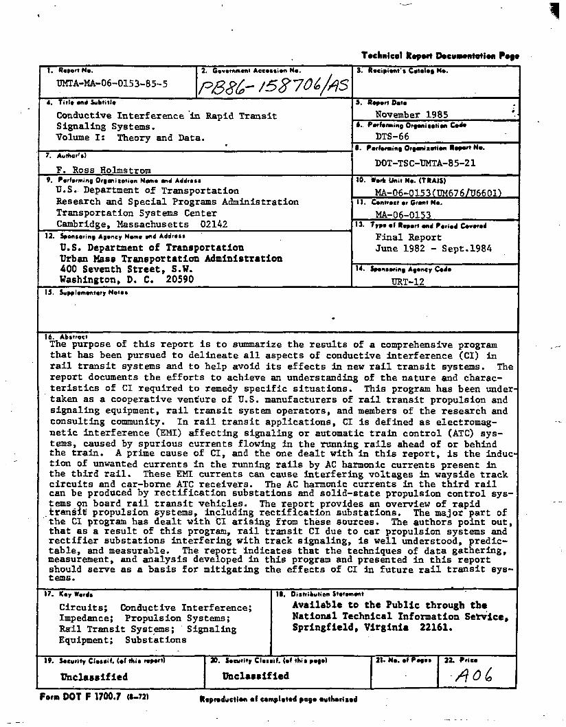
4. Title en4 SubtitleConductive Interference in Rapid Transit Signaling Systems.Volume I: Theory and Data.

5. Regert DeteNovember 1985t. Perfenaing Orgenisetien Ce4eDTS-66

7. Author'*)F. Ross Holmstrom

I. Performing Orgenisetien Regert Ne.DOT-TS C-UMTA-8 5-21

9. Performing Organisation Name md Addrat*U.S. Department of Transportation Research and Special Programs Administration Transportation Systems Center Cambridge* Massachusetts 02142 ___

10. Werft Unit Ne. (TRAIS)MA-06-0153(’PM676/U6601’>11. Centrect er Orent Ne.MA-06-0153

12. Spans ■ Name and AddressU.S. Department of Transportation Urban Mass Transportation Administration 400 Seventh Street* S.W.Washington* D. C. 20590

13. Type ef Repert end Peried CoveredFinal ReportJune 1982 - Sept.1984

14. Sponsoring Agency CedeURT-1215. Supplementary Notts

16. AbstroctThe purpose of this report is to summarize the results of a comprehensive program that has been pursued to delineate all aspects of conductive interference (Cl) in rail transit systems and to help avoid its effects in new rail transit systems. The report documents the efforts to achieve an understanding of the nature and characteristics of Cl required to remedy specific situations. This program has been under taken as a cooperative venture of U.S. manufacturers of rail transit propulsion and signaling equipment, rail transit system operators* and members of the research and consulting community. In rail transit applications, Cl is defined as electromagnetic interference (EMI) affecting signaling or automatic train control (ATC) systems, caused by spurious currents flowing in the running rails ahead of or behind the train. A prime cause of Cl, and the one dealt with in this report, is the indue tion of unwanted currents in the running rails by AC harmonic currents present in the third rail. These EMI currents can cause interfering voltages in wayside track circuits and car-borne ATC receivers. The AC harmonic currents in the third rail can be produced by rectification substations and solid-state propulsion control systems pn board rail transit vehicles. The report provides an overview of rapid transit propulsion systems* including rectification substations. The major part of the Cl program has dealt with Cl arising from these sources. The authors point out, that as a result of this program* rail transit Cl due to car propulsion systems and rectifier substations interfering with track signaling, is well understood* predictable, and measurable. The report indicates that the techniques of data gathering* measurement, and analysis developed in this program and presented in this report should serve as a basis for mitigating the effects of Cl in future rail transit systems.17. Kay Wards

Circuits; Conductive Interference; Impedance; Propulsion Systems; Rail Transit Systems; Signaling Equipment; Substations

II. Distribution StatementAvailable to the Public through the National Technical Information Service, Springfield* Virginia 22161.

19. Security Classil. (el this rogart)Unclassified

20. Security Clessil. (el this gage)Unclassified

21. Ne. el Pages 22. PriceAOC,

F.m DOT F 1700.7 «-?» Reproduction el completed page euthorised

Technical Report Documentation Page

!• Report No.UMTA-MA-06-0153-85-5

2. Government Accession No. 3. Recipient s Catalog No.

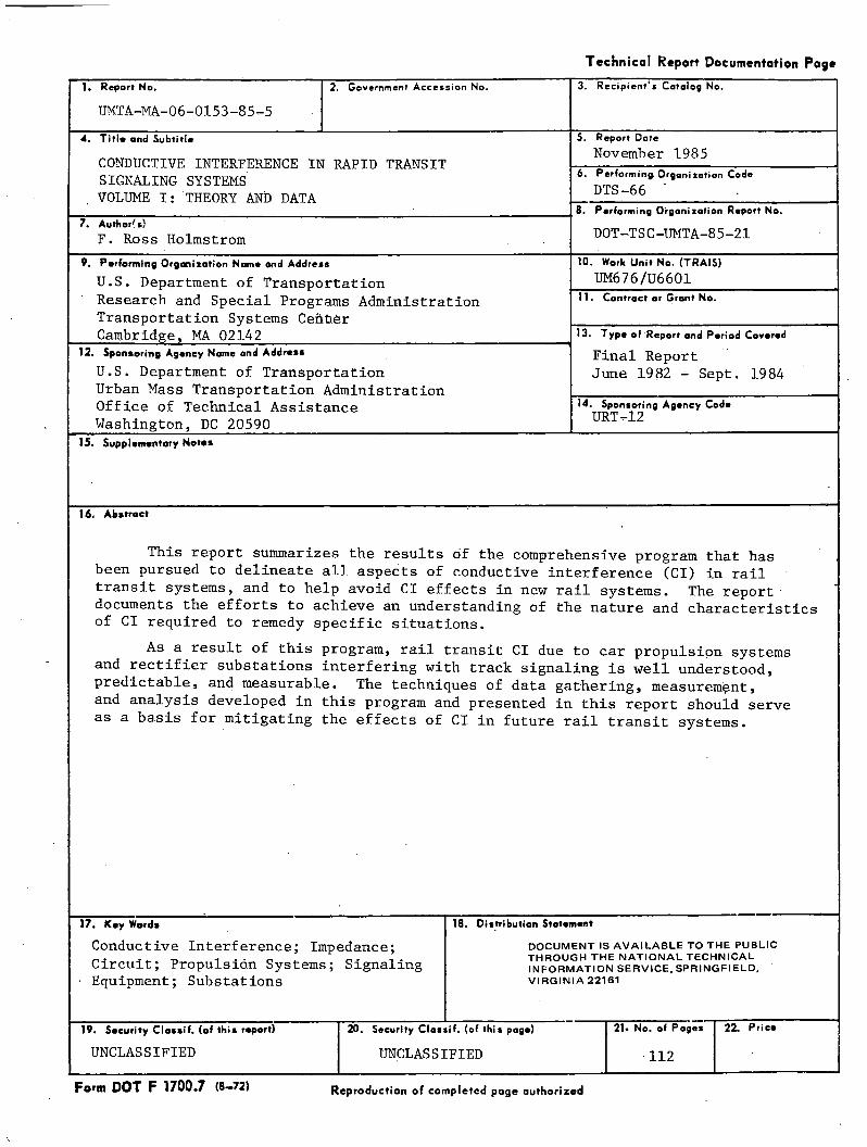
4. Title and SubtitleCONDUCTIVE INTERFERENCE IN RAPID TRANSITSIGNALING SYSTEMSVOLUME I: THEORY AND DATA

5. Report DateNovember 1985

6. Performing. Orgoniration CodeDTS-66 ‘

6. Performing Organization Report No.DOT-TSC-UMTA-85-217. Author's)

F. Ross Holmstrom9. Performing Organization Name and Address

U.S. Department of Transportation Research and Special Programs Administration Transportation Systems CeftfcSr Cambridge, MA 02142

10. Work Unit No. (TRAIS)UM676/U6601

11. Contract or Grant No.

13. Type of Report and Period CoveredFinal ReportJune 1982 - Sept. 1984

12. Sponsoring Agency Name and AddressU.S. Department of Transportation Urban Mass Transportation Administration Office of Technical Assistance Washington, DC 20590

14. Sponsoring Agency CodeURT-12

15. Supplementary Note*

16. Abstract

This report summarizes the results djf the comprehensive program that has been pursued to delineate all aspects of conductive interference (Cl) in rail transit systems, and to help avoid Cl effects in new rail systems. The report documents the efforts to achieve an understanding of the nature and characteristics of Cl required to remedy specific situations.

As a result of this program, rail transit Cl due to car propulsion systems and rectifier substations interfering with track signaling is well understood, predictable, and measurable. The techniques of data gathering, measurement, and analysis developed in this program and presented in this report should serve as a basis for mitigating the effects of Cl in future rail transit systems.

17. Key Words 18. Distribution StatementConductive Interference; Impedance; Circuit; Propulsion Systems; Signaling

■ Equipment; Substations

DOCUMENT IS AVAILABLE TO THE PUBLIC THROUGH THE NATIONAL TECHNICAL INFORMATION SERVICE, SPRINGFIELD, VIRGINIA 22161

19. Security Classif. (of this report) 20. Security Classif. (of this page) 21« No. of Pages 22. PricaUNCLASSIFIED UNCLASSIFIED 112

Form D O T F 1700.7 (8-72) Reproduction of completed page authorized

PREFACE

This report summarizes the results of the comprehensive program that has been pursued to delineate all aspects of conductive interference in rail transit systems, and to help avoid its effects in new rail transit systems. The program has been undertaken as a cooperative venture of U.S. manufacturers of rail transit propulsion and signaling equipment, rail transit system operators, and members of the research and consulting community, under the aegis of the Rail Transit EMI/EMC Working Group, sponsored by the Urban Mass Transportation Administration of the U.S. Department of Transportation.

This effort has enjoyed the direct and indirect efforts of many people. In addition to Messrs. Krempasky, Clark, Frasco, Hoelscher, Rudich, and Truman, who are noted in the References section of this report, the author wishes to express gratitude to Lennart Long of DOT/TSC, whose encouragement, support, and personal involvement were directly instrumental in the completion of this project. Charles Edelson, then of SDC, Inc., was an active participant in many of the tasks reported on here. Donald Stark of Union Switch & Signal Div., American Standard, Inc., suggested to the author the form of the lumped equivalent circuit shown in Sec. 6, and provided much useful information on the nature of conductive interference in the real world. Tatiana Vinnikova, then of SDC, Inc., was instrumental in the computation of probability integrals in Section 8. The personnel of the Massachusetts Bay Transit Authority (MBTA) gave invaluable assistance for the rail impedance tests described in Sections 3-5, as did Irving Golini, Michael West, John Lewis, and Paul Poirier of DOT/TSC, and Klaus Frielinghaus of GRS, Inc. Bay Area Rapid Transit District (BART) personnel expended immense effort and hospitality to make the multi-car measurements outlined in Section 9 possible. Final thanks go to the sponsor of the UMTA program in rail transit EMI/EMC - Ronald Kangas, Chief of the Design Division, UMTA Office of Systems Engineering.

— i i i —

METRIC CONVERSION FACTORS

Approximate Conversionsto Metric Measures

Symbol When You Know Multiply by To Find Symbol 8LENGTH

in inches •2.6 centimeters cmit feet 30 centimeters cmyd yards 0.8 meters m --=mi miles 1.6 kilometers kmAREA — E

—in2 squire inches 6.6 square centimeters cm* — ~~ft* square feet 0.09 square meters m2 —yd2 square yerds OS square meters m2 —mi* square miles 2.6 square kilometers km* __—acres 0.4 hectares ha 6— '“Ul

MASS (weight) ililil

OS ounces 28 grams 8lb pounds 0.46 kilograms kgshort tons OA tonnes t 4—(20001b) -EVOLUME -E

tsp teaspoons 6 milliliters ml — =Tbsp tablespoons 16 milliliters ml 3-- ~~fl oz fluid ounces 30 milliliters mlc cups 0.24 liters i —pt pints 0.47 liters i ----Eqt quarts 0.95 liters i — ~gal gallons 3.8 liters ift* cubic feat 0.03 cubic meters m3 2 —yd3 cubic yards 0.76 cubic maters m3 __~

TEMPERATURE (exact)°F Fahrenheit 5/9 (after Celsius °c — —

temperature subtracting temperature 1-- -

32) T1 In. - 2.64 cm (exactly). For other ax act convaralona and more detail tablet aaa ~NBS Mite. Publ. 266. Unit* of Weight and Maasurea. Price $2.25 SO Catalog No. CIS 10 286. inches

-23Approximate Conversions fromi Metric Measures

-22-21 Symbol When You Know Multiply by To Find Symbol

-20 LENGTH

-19 mm millimeters 0.04 inches incm centimeters 0.4 inches in-18 m meters 3.3 feet nm meters 1.1 yards yd-17 km kilometers 0.6 miles mi

-16 AREA

-16 cm* square centimeters 0.16 square inches in2m2 square meters 1.2 square yards yd*-14 km* square kilometers 0.4 square miles mi2ha hectares (10,000 m*) 2.5 acres-13

MASS (weight)

-11 g grams 0.035 ounces OZ

kg kilograms 2.2 pounds lbt tonnes (1000 kg) 1.1 short tons-10-9 VOLUME

-8 ml milliliters 0.03 fluid ounces fl ozi liters 2.1 pints Pti liters 1.06 quarts qt— 7 i liters 0.26 gallons galm3 cubic meters 36 cubic feet ft*-6 m3 cubic meters 1.3 cubic yards yd*

-5 TEMPERATURE (exact)-4 °c Celsius 9/5 (then Fahrenheit °Ftemperature add 32) temperature-3

°F-2 °F 32 98.6 212

-40 0 1 1 1 1 1 l 1 140 80 ll 1 | 1 1 II 1 120 160 1 1 t 1 i 1 1 l 1 2001 i 1 11 r i i

-40 -20 1 20fl 1 T T 1 |40 60 80 1 1 100cm °c 0 37 °c

TABLE OF CONTENTS

1. INTRODUCTION. . . . . . . . . . . . . . . . . . . . . . . . . . . . . . . . . 12. THE CONDUCTIVE INTERFERENCE MODEL . . . . . . . . . . . . . . . . . . . . 33. DEPENDENCE OF AC RAIL IMPEDANCE ON FREQUENCY AND DC CURRENT . . . 6

3.1 Electromagnetic Properties of Steel Rails . . . . . . . . . . . . 63.2 Measurement of AC Rail Resistance and Inductance . . . . 63.3 Rail Resistance and Inductance Data, and Track Impedance . . 10

4. COMPARISON OF CALCULATED AND MEASURED TRACK IMPEDANCE . . . . . . . . 175. MEASURED RAIL IMPEDANCE VS. SKIN EFFECT T H E O R Y . . . . . . . . . . . . 23

5.1 Skin Effect Theory - the Skin Depth Parameter. . . . . . . 235.2 Skin Effect in Conductors of Circular Crossection . . . . 245.3 Skin Effect in Railroad R a i l . . . . . . . . . . . .. 275.4 Conclusions. . . . . . . . . . . . . . . . . . . . . . . . . . . . . .. 32

6. CIRCUIT ANALYSIS OF TRACK WITH THIRD RAIL, TRACK CIRCUITS AND BALLAST 336.1 The M o d e l . . . . . . . . . . . . . . . . . . . . . . . . . . . . . . . 336.2 Double-Rail Track Circuit . . . . . . . . . . . . . . . . . . . . . . 336.3 Differential Equations for Circuit . . . . . . . . . . . . . . . . 366.4 An Equivalent Lumped Circuit. . . . . . . . . . . .. 406.5 Single-Rail Track Circuits . . . . . . . . . . . . . . . . . . . . . . 426.6 Overall Result for Coupling from Third Rail . . . . . . . . . . 446.7 The Conductive Interference Current Transfer Function . . . 446.8 Sample Calculations . . . . . . . . . . . . . . . . . . . . . . . . . . 466.9 Impedance of the Third Rail-DC Return Circuit -

Balanced 2-Rail Case .. . . . . . . . . . . . . . . . . . . . . 466.10 Impedance of the Third Rail-DC Return Circuit -

Single Rail Adjacent to Third R a i l . . . . . . . . . . . . . . . . 526.11 Impedance of the Third Rail-DC Return Circuit -

DC Return Rail Adjacent to Third R a i l . . . . . . . . . . . . . . 536.12 Rail Data to Use in Computation. . . . . . . . . . . . . . . . . 546.13 Summary & Conclusions .. . . . . . . . . . . . . . . . . . . . . . . . . . . 55

Page

-v-

TABLE OF CONTENTS (cont'd)

7. INTERFERENCE SOURCE CHARACTERISTICS OF MULTI-CAR TRAINS:CIRCUIT EFFECTS . . . . 567.1 The Multi-Car Source . . . . . . . . . . . . . . 567.2 The Equivalent Circuit of a Multi-Car Train . . . . . . . . . . 567.3 Summary & Conclusions . . . . . 63

8. INTERFERENCE SOURCE CHARACTERISTICS OF MULTI-CAR TRAINS:STATISTICS .. . . . . . . . . . . . . . . . . . . . . . . . . . . . . . . . . . 648.1 Statistical Properties . 648.2 Probability Density Functions . . 658.3 Statistical Results . . . . . . . . . . . . . . . . . . . . . . . . . . 698.4 Behavior for Large Values of n . . . . . . . . . . . . . 718.5 Probability of r Exceeding a Particular Value .... 718.6 Extension to the Case of Unequal Contributions From n Cars . 748.7 Statistics Summary . 75

9. MEASUREMENT OF CONDUCTIVE INTERFERENCE: TECHNIQUES & DATA . . . 769.1 Recommended Practices .. . . . . . . . . . . . . . . . . . . . . . . 769.2 Instrumentation . . . . . . . . . . . . . . . . . . . . 769.3 Representative Data from one Rapid Transit Car . . . . . 779.4 Conductive Interference Data From Multi-Car Trains . . . . 819.5 Summary. . . . . . . . . . . . . . . . 92

10. CONCLUSION. . . . . . . . . . . . . . . . . . . . . . . . . . . . . . . . . 94APPENDIX: FORTRAN PROGRAM FOR CALCULATING THE CONDUCTIVE

INTERFERENCE TRANSFER FUNCTION . . . . . . . . . . A.1REFERENCES . . . .. . . . . . . . . . . . . . . . . . . . . . . . . . . . . . . . . . R.l

- v i -

FIGURES

Figure Page

2.1 The conductive interference model ......................... 43.1 The circuit for measuring impedance properties of rail . . . . 83.2 The transmission-line model of railroad track ............... 124.1 Waves on a transmission line.................................194.2 Transmission line series resistance for railroad track . . . . 214.3 Transmission line series inductance for railroad track . . . . 225.1 Resistance and internal reactance for solid circular conductors . 265.2 AL vs. f-1 for 200 Ib/yd running rail ....................... 295.3 a L v s. f-1^ for 150 lb/yd high-conductivity third rail,

for three values of dc current........................... 306.1 The coupled transmission line model of running rails and third rail 346.2 Currents and voltages in the balanced double-rail track circuit 356.3 Magnetic coupling between third rail and running rails . . . . 376.4 An incremental portion of the third rail and running rails . . . 386.5 The lumped-element pi-circuit that is equivalent to the

transmission line formed by the running rails ............... 416.6 The lumped-element pi-circuit with coupling from third rail included 416.7 The lumped-element pi-circuit with third-rail coupling and

receiver impedances added ................................ 416.8 Series impedance model of track circuits and third rail in the

substation-to-train loop ................................ 486.9 Series impedance of one track circuit and adjacent third rail . . 497.1 Equivalent circuit for conductive interference generation in a

multi-car train ........................................ 577.2 The conductive interference circuit showing train, circuit

inductance, and substation................... 628.1 Addition of randomly oriented phasors ...................... 668.2 The strip in the (r',c) plane where r < R < r+dr............... 688.3 Probability density functions pk(r) for sums of k randomly

oriented unit phasors, for k = 1, ..., 8 .................... 70

- v i i -

FIGURES (cont'd)

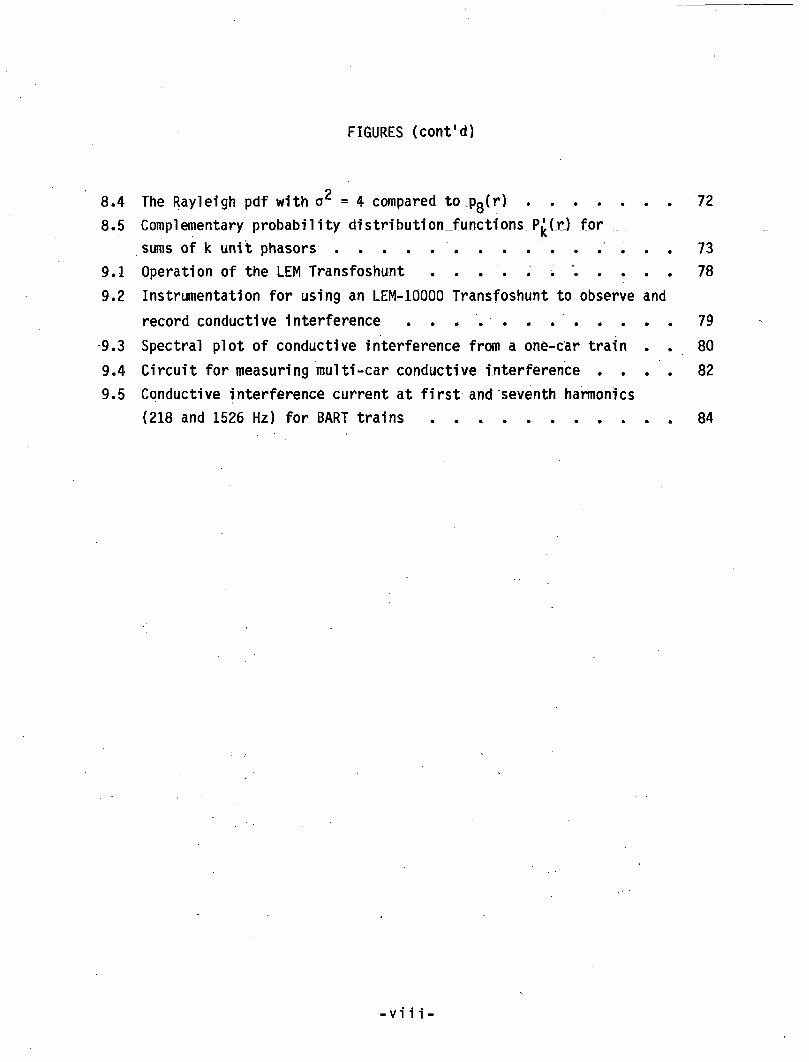
8.4 The Rayleigh pdf with a2 = 4 compared to.p8(r) ............... 728.5 Complementary probability distribution_functions P£(n)_ for .

sums of k unit phasors............ 739.1 Operation of the LEM Transfoshunt ......................... 789.2 Instrumentation for using an LEM-10000 Transfoshunt to observe and

record conductive interference . . . . . . . .......... 799.3 Spectral plot of conductive interference from a one-car train . . 8 09.4 Circuit for measuring multi-car conductive interference . . . . 829.5 Conductive interference current at first and seventh harmonics

(218 and 1526 Hz) for BART trains ......................... 84

- v i i i -

TABLES

Table Page

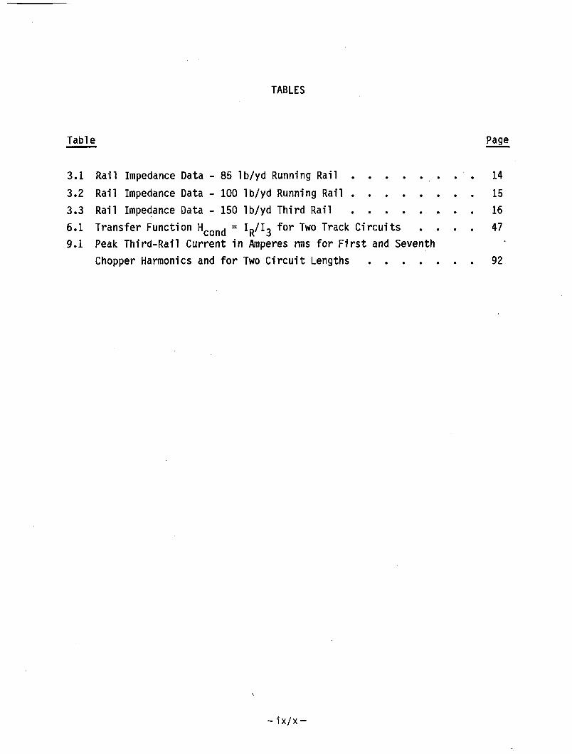
3.1 Rail Impedance Data - 85 lb/yd Running Rail............. 143.2 Rail Impedance Data - 100 lb/yd Running Rail.................... 153.3 Rail Impedance Data - 150 lb/yd Third R a i l .................... 166.1 Transfer Function Hcond = IR/I3 for Two Track Circuits . . . . 479.1 Peak Third-Rail Current in Amperes rms for First and Seventh

Chopper Harmonics and for Two Circuit Lengths ............... 92

- ix/x -

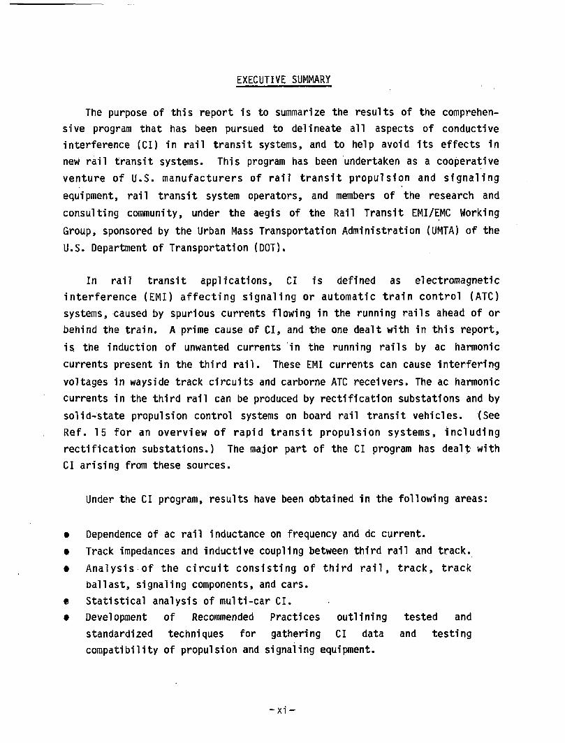
EXECUTIVE SUMMARY

The purpose of this report is to summarize the results of the comprehensive program that has been pursued to delineate all aspects of conductive interference (Cl) in rail transit systems, and to help avoid its effects in new rail transit systems. This program has been undertaken as a cooperative venture of U.S. manufacturers of rail transit propulsion and signaling equipment, rail transit system operators, and members of the research andconsulting community, under the aegis of the Rail Transit EMI/EMC WorkingGroup, sponsored by the Urban Mass Transportation Administration (UMTA) of the U.S. Department of Transportation (DOT).

In rail transit applications, Cl is defined as electromagnetic interference (EMI) affecting signaling or automatic train control (ATC) systems, caused by spurious currents flowing in the running rails ahead of or behind the train. A prime cause of Cl, and the one dealt with in this report,is. the induction of unwanted currents in the running rails by ac harmoniccurrents present in the third rail. These EMI currents can cause interfering voltages in wayside track circuits and carborne ATC receivers. The ac harmonic currents in the third rail can be produced by rectification substations and by solid-state propulsion control systems on board rail transit vehicles. (See Ref. 15 for an overview of rapid transit propulsion systems, including rectification substations.) The major part of the Cl program has dealt with Cl arising from these sources.

Under the Cl program, results have been obtained in the following areas:

• Dependence of ac rail inductance on frequency and dc current.t Track impedances and inductive coupling between third rail and track.• Analysis of the circuit consisting of third rail, track, track

ballast, signaling components, and cars.• Statistical analysis of multi-car Cl.• Development of Recommended Practices outlining tested and

standardized techniques for gathering Cl data and testingcompatibility of propulsion and signaling equipment.

- xi

This report documents the efforts to achieve the understanding of the nature and characteristics of Cl that is required for intelligent application of the Cl Recommended Practices to specific situations.

As a result of this program, rail transit Cl due to car propulsion systems and rectifier substations interfering with track signaling and ATC systems, is well understood, predictable, and measureable. The techniques of data gathering, measurement, and analysis developed in this program and presented in this report should serve as a basis for mitigating the effects of Cl in future rail transit systems.

1.0 INTRODUCTION

Rapid transit systems in the U.S. traditionally have used dc propulsion control systems relying on switched field resistors and windings. Their signaling systems have been based on power-frequency track circuits and wayside signals. In recent years the desire for greater operational efficiency has led to the introduction of advanced audio-frequency automatic train control (ATC) and signaling systems, and new types of propulsion control systems. Advanced electronics are used in both the new ATC systems and propulsion control systems.

Audio-frequency ATC systems can be installed on continuously welded rail, thus obviating the need for insulated joints. In addition, such systems allow easy integration of train detection and transmission of ATC signals to the train.

Propulsion control systems using switched thyristors eliminate the moving parts and electrical contactors that prove to be high-maintenance items in older dc propulsion control systems. In the future, the U.S. may see a further advancement now used in Europe and Japan - ac induction motors with electronically controlled dc-to-ac converters. These will replace the dc traction motors and their commutator rings and brushes. [Ref. 15]

To realize the advantages these modern electronic systems, their electromagnetic compatibility (EMC) must be assured. Early U.S. tests showed that propulsion systems with solid-state control can cause audio-frequency harmonic currents to flow in the third and running rails and into track circuit receivers. The problems of this electromagnetic interference (EMI) can be solved,* but solution requires thorough understanding of the mechanisms involved, and a coordinated design of the ATC and propulsion systems.

The U.S. Department of Transportation's EMI/EMC program has the objective of assuring the EMC of rail transit electrical and electronic subsystems. Major goals of this program are to:

-1-

• Develop and validate Recommended Practices (RP's) for measuring EMI and susceptibility of rail transit electrical and electronic subsystems.

• Provide EMI/EMC support to the UMTA/STARS New Technology Assessment and Development Program.

• Develop engineering guidelines for transit authorities and suppliers, to aid in the evaluation and elimination of EMI that could cause safety or operational problems.

• Coordinate and support the activities of the International Rail Transit EMI/EMC Technical Working Group (TWG), and support the APTA/EMI Liaison Board.

The purpose of the RP's is to have a set of test procedures with industrywide acceptance that can provide a common framework for eliminating and avoiding EMI problems and assuring EMC. To date, two sets of RP's have been developed and have been released to the IEEE for their consideration as new standards [Ref. 12]. These sets deal with two specific types of EMI - Inductive and Conductive.

As defined in rail transit, inductive EMI results from stray ac magnetic fields from a car's propulsion or auxiliary power system inductively coupling to the conducting loops under the car comprised of signal receiver leads, rails, and car axles. Conductive EMI, the topic of this report, results from the injection of ac harmonic currents from substation or car into the conducting loop formed by the third rail and running rails, and thence into signal receiver leads attached to the running rails.

-2-

2. THE CONDUCTIVE INTERFERENCE MODEL

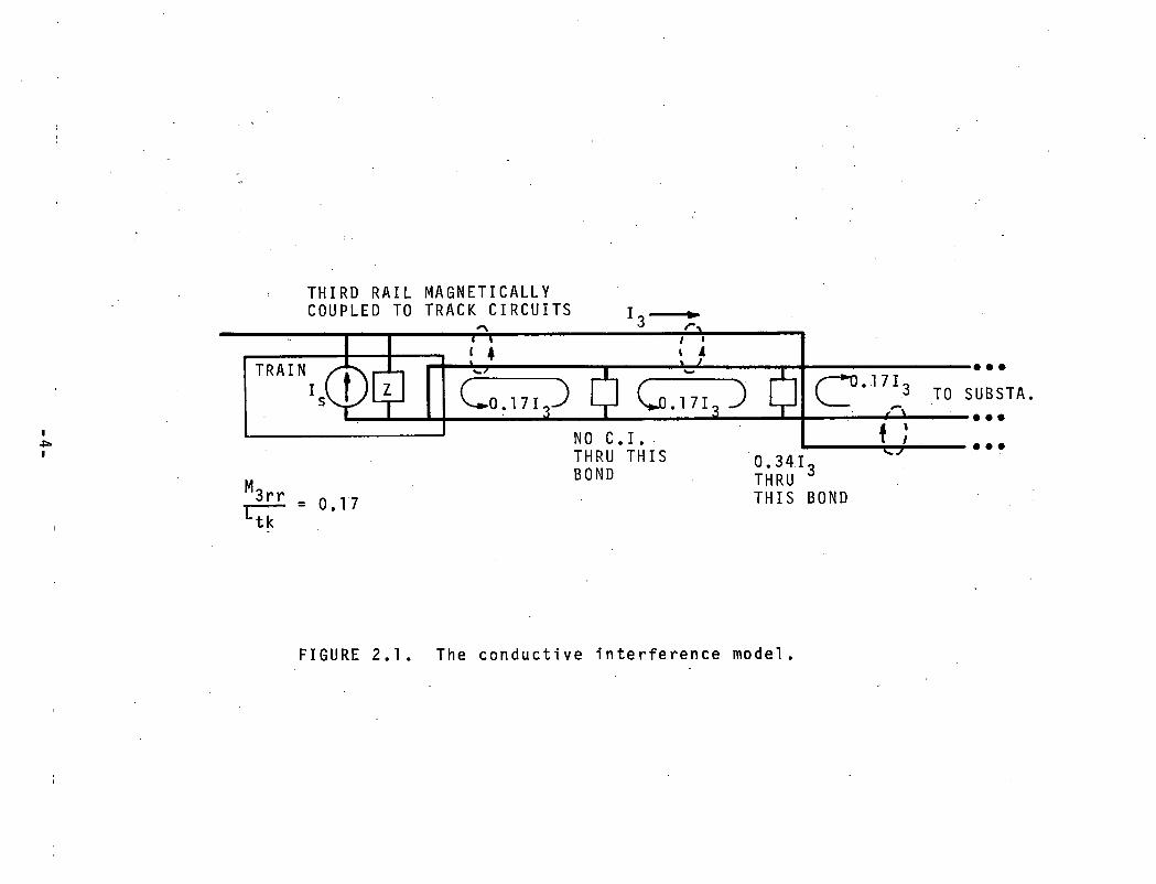
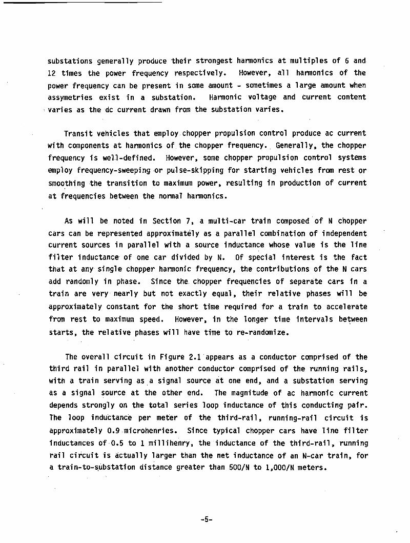
This section summarizes the analysis of conductive interference in rapid transit systems. Figure 2.1 shows the configuration of third rail, running rails, train, and substation that can lead to the induction of Cl currents into the running rails. This figure shows balanced 2-rail audio-frequency track circuits with continuously welded rail. The third rail is positioned assymetrically with respect to the running rails, leading to non-zero mutual inductance between the third rail and the loop formed by the running rails. If an overhead catenary were used to carry dc current to the train, and if it were positioned exactly above the centerline of the running rails, the mutual inductance from it to the running rail loop would be zero.

Cl currents induced into the running rails do not necessarily result in currents into track circuit receivers shunting the running rails. In the example in Figure 2.1, if the third rail runs continuously down one side of the track, equal but opposite currents through a track circuit receiver will flow due to currents induced into the loops to the left and to the right of the receiver, giving a net Cl current of zero. However, if the third rail is switched from one side of the track to the other at the location of a track circuit receiver, the Cl current in the track circuit receiver can be as great as twice the circulating or differential-mode Cl current in the rails. Therefore, the layout of the third-rail circuit can have a direct impact on Cl — a fact that track designers should be aware of.

A detailed analysis of this circuit must also include the impedances of track circuit components, and the leakage conductance of the track ballast. As will be shown in Section 6, a good rule-of-thumb for the ratio of third-rail ac current to induced differential mode current in the running rails is the ratio of self-inductance per meter of the running rail loop to the mutual inductance per meter between third rail and the running rail loop. This ratio is approximately 6:1.

Substations serve as one source of ac current in the third rail. Substations generally behave as practically ideal voltage sources with very low source impedance. Three-phase and six-phase full-wave rectifier

-3-

THIRD RAIL MAGNETICALLY

FIGURE 2.1 The conductive interference model

substations generally produce their strongest harmonics at multiples of 6 and 12 times the power frequency respectively. However, all harmonics of the power frequency can be present in some amount - sometimes a large amount when assymetries exist in a substation. Harmonic voltage and current content varies as the dc current drawn from the substation varies.

Transit vehicles that employ chopper propulsion control produce ac current with components at harmonics of the chopper frequency. Generally, the chopper frequency is well-defined. However, some chopper propulsion control systems employ frequency-sweeping or pulse-skipping for starting vehicles from rest or smoothing the transition to maximum power, resulting in production of current at frequencies between the normal harmonics.

As will be noted in Section 7, a multi-car train composed of N chopper cars can be represented approximately as a parallel combination of independent current sources in parallel with a source inductance whose value is the line filter inductance of one car divided by N. Of special interest is the fact that at any single chopper harmonic frequency, the contributions of the N cars add randomly in phase. Since the. chopper frequencies of separate cars in a train are very nearly but not exactly equal, their relative phases will be approximately constant for the short time required for a train to accelerate from rest to maximum speed. However, in the longer time intervals between starts, the relative phases will have time to re-randomize.

The overall circuit in Figure 2.1 appears as a conductor comprised of the third rail in parallel with another conductor comprised of the running rails, with a train serving as a signal source at one end, and a substation serving as a signal source at the other end. The magnitude of ac harmonic current depends strongly on the total series loop inductance of this conducting pair. The loop inductance per meter of the third-rail, running-rail circuit is approximately 0.9 microhenries. Since typical chopper cars have line filter inductances of 0.5 to 1 millihenry, the inductance of the third-rail, running rail circuit is actually larger than the net inductance of an N-car train, for a train-to-substation distance greater than 500/N to 1,000/N meters.

-5-

3. DEPENDENCE OF AC RAIL IMPEDANCE ON FREQUENCY AND DC CURRENT

3.1 Electromagnetic Properties of Steel Rails

To calculate expected values of harmonic currents and voltages in the circuit of Figure 2.1, the impedance characteristics of the circuit must be known. These characteristics depend upon the self and mutual inductances of the rails due to ac magnetic flux outside the rails, and upon the contribution to rail impedance due to rail resistance and due to ac magnetic flux beneath the surface of the rails. Since the rails are ferromagnetic, rail inductance and resistance are functions of dc current as well as frequency.

The ac magnetic field beneath the surface of the rail decreases approximately exponentially with depth into the rail, with an attenuation coefficient defined as the skin depth. The magnetic permeability of steel is many times greater than that of aluminum or copper. . However, steel's conductivity is many times less, and therefore the skin depth in steel and aluminum or copper are roughly comparable. However, the presence of ac magnetic fields within the high-permeability steel leads to an increase in total circuit inductance. The contribution to inductance due to ac magnetic fields within the steel will be referred to here as the "internal inductance."

Since skin depth is smaller when magnetic permeability is greater, the audio-frequency resistance of steel rail is significantly greater than that of aluminum or copper conductors of equivalent crossection.

3.2 Measurement of AC Rail Resistance and Inductance

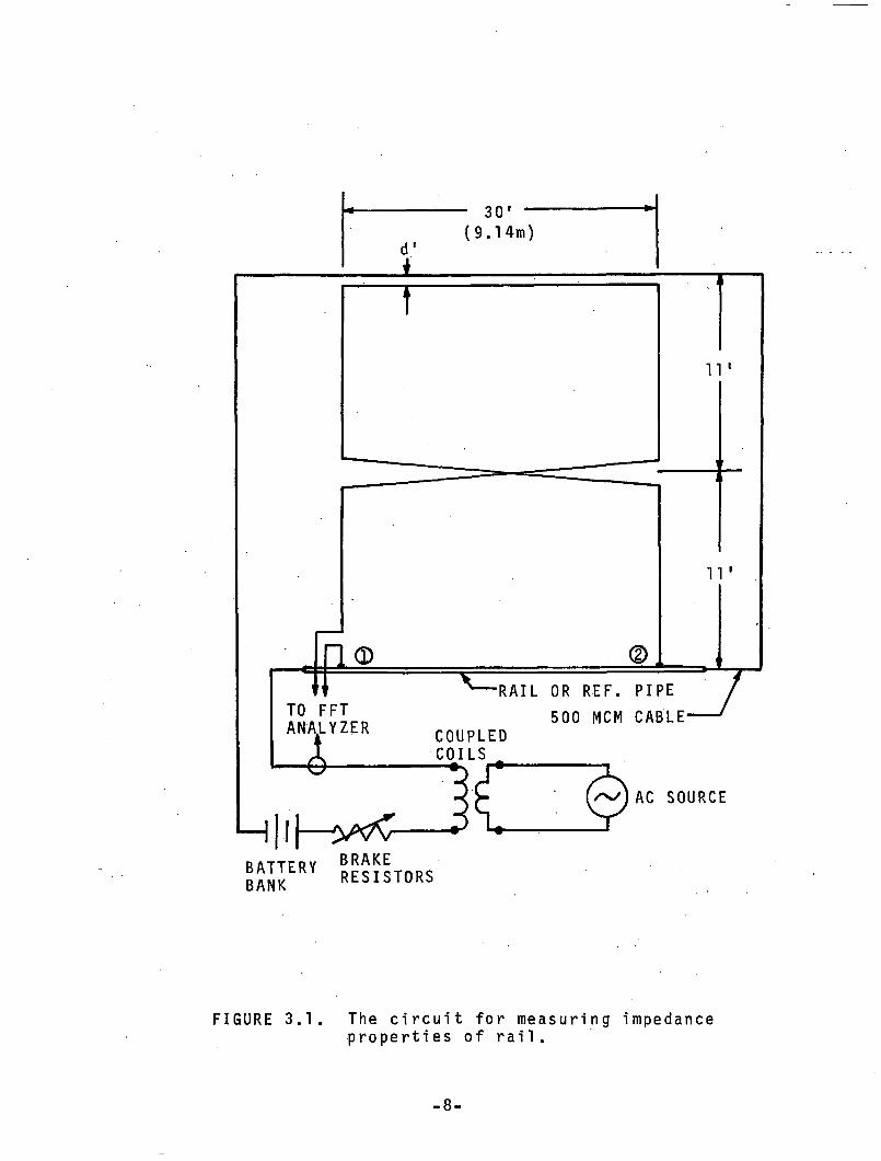
A series of measurements was conducted to determine the variation of internal small-signal ac inductance of railroad rail as a function of frequency and dc current. The frequency range was from 25 Hz to 3 kHz, and the dc current range was from 0 to approximately 1,000 amperes. This range of dc current is broader than that previously investigated by Holland-Moritz, who made similar measurements [Ref. 1]. The configuration of the circuit employed is shown in Fig. 3.1. This circuit is an adaptation of one used by Kennelly, Achard & Dana, to investigate variation of large-signal ac inductance at power

- 6 -

frequencies [Ref. 2]. The difference lies in the addition of the upper loop in the voltage sensing conductor pair, resulting in a nulling circuit.

In the circuit shown in Fig. 3.1, the dc current source was a parallel bank of storage batteries from motor buses. DC current was controlled by a bank of switched brake resistors from rail transit cars. The ac coupling transformer secondary winding was a solenoidal motor smoothing reactor from a rapid transit car. The primary winding was formed by wrapping 20 turns of No. 20 AWG wire around the motor smoothing reactor.

A servo-type Hall Effect electronic current transformer (see Sec. 9.2) was employed to simultaneously measure dc and ac current in the rail. The turns ratio of the current transformer was 5,000:1, and a 10-ohm sensing resistor was used, resulting in a transresistance ratio Vsense/Is = (1/500) ohm.

A digital voltmeter was used to observe the dc component of Vsense. Theac signal source was a digitally controlled sine-wave oscillator of extremefrequency stability. A two-channel FFT network analyzer was used in thetransfer function mode to observe the amplitude and phase of VQ/Vsense atspecific frequencies. Measurement frequencies were chosen that correspondedexactly to FFT frequency lines. The FFT analyzer served as a two-channeldigital filter for providing adequate signal-to-noise ratio. Signal-to-noiseratio for V and V was directly observed by using the FFT analyzer in the o sensesingle-channel mode to compare the amplitude of VQ and Vs to amplitudes of interference present at other displayed FFT frequencies. In all cases, signal-to-noise ratio was better than 20 db.

The circuit of Fig. 3.1 was used in the following manner: First, a lengthof copper pipe with 1-5/8 inch outer diameter, serving as the reference conductor, was placed in the position where the rail was to go, referred to hereafter as the test conductor position. Then, ac current was applied to the loop containing the copper pipe, and spacing d‘ between the return conductor and the nulling conductor was adjusted to provide the lowest possible magnitude of induced voltage V0, at a frequency of 1,000 Hz.

-7-

r*J) AC SOURCEH | J [ —

BATTERYBANKBRAKERESISTORS

FIGURE 3.1. The circuit for measuring impedance properties of rail.

-8-

The copper pipe had a wall thichness much less than its radius. Therefore to a good approximation, the current in the copper reference conductor can be considered a sheet current. An analysis of the geometry of the sensing loop and the magnetic flux field of the current loop shows that the net flux linkages of the sensing loop is exactly zero, provided that d' = ^ .Therefore, in the absence of ac resistance in the copper pipe, it would have been possible to make VQ exactly zero, when the copper pipe reference conductor was in place.

It was not neccesary to make the actual spacing between return and nulling conductors exactly uniform over their length, since VQ only depends on total flux intercepted, and not its distribution. However, it was necessary to leave the positions of return and nulling conductors undisturbed after the best-case null for VQ was obtained.

After the above circuit adjustment, the copper pipe was removed andreplaced by 40-foot lengths of railroad rail of a number of crossections.When another test conductor replaces the reference conductor, the magneticflux linkages passing through the sensing loop change, due to the differentsize, crossectional shape, and composition of the new conductor. Theinductive part of VQ is due to the difference between the reactances of thetest conductor and reference conductor. The resistive part of V is due toothe ac resistance of the test conductor.

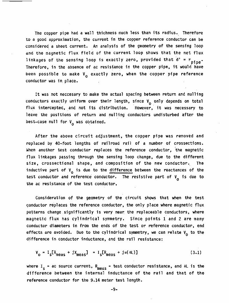
Consideration of the geometry of the circuit shows that when the test conductor replaces the reference conductor, the only place where magnetic flux patterns change significantly is very near the replaceable conductors, where magnetic flux has cylindrical symmetry. Since points 1 and 2 are many conductor diameters in from the ends of the test or reference conductor, end effects are avoided. Due to the cylindrical symmetry, we can relate VQ to the difference in conductor inductance, and the rail resistance:

Vo - ^^neas + jXmeas^ ” ^^meas + (3.1)where I,. = ac source current, R = test conductor resistance, and AL is the

S fTicaSdifference between the internal inductance of the rail and that of the reference conductor for the 9.14 meter test length.

-9-

It is important to observe in Eqn. 3.1, that VQ depends on the difference between internal inductances of the rail and the copper pipe, and not the value of either itself. Furthermore, the term internal inductance implies inductance due to magnetic flux inside some reference surface, as oppoised to the external inductance due to magnetic flux outside the surface. We can change the values of internal inductance of both the reference conductor and test conductor by choosing a new reference surface; however, this does not change their differences. As a matter of convenience, we have defined the internal inductance of the reference conductor to be zero.

As will be seen in the data to follow, al will be positive at very low frequencies, due to internal magnetic fields, but negative at very high frequencies where the skin effect excludes magnetic fields from the interior of the rail. As noted above, this difference is due to magnetic field behavior within a few test conductor diameters of the test and reference conductors. As is discussed in Section 3.3 below, the value of this difference can be used in conjunction with the known properties of copper pipe to directly calculate the inductance per meter of railroad track composed of two running rails.

3.3 Rail Resistance and Inductance Data, and Track Impedance

Using the circuit of Fig. 3.1, data were collected for 85 lb/yd running rail, 100 lb/yd running rail, and 150 lb/yd NYCTA third rail. Data for dc currents between zero and appx. 1,000 amperes and frequencies between 25 and 3160 Hz are shown in Tables 3.1, 3.2, and 3.3. Included in Tables 3.1 and 3.2 are values of total track resistance and inductance per meter, calculated on the basis; of the the measured impedance properties of individual pieces of rail.

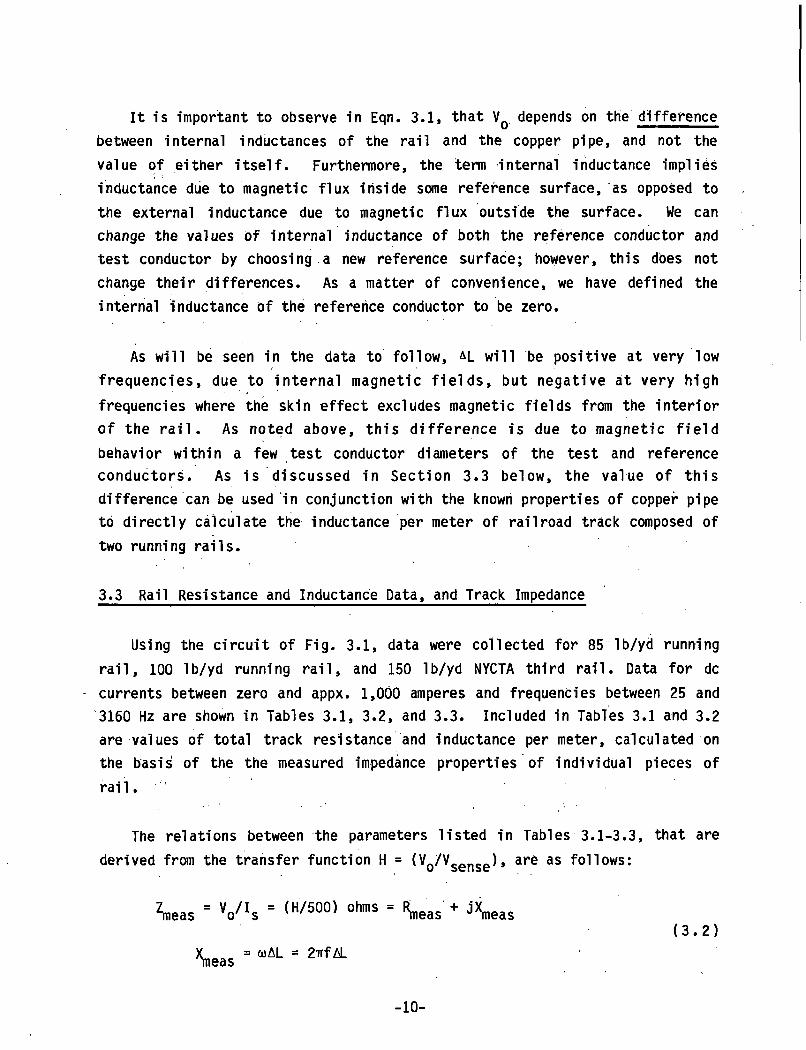
The relations between the parameters listed in Tables 3.1-3.3, that are derived from the transfer function H = (v0/vsense^’ are as foll°ws:

W - V 1* - (H/500' ohms - "meas + ‘V a s

eas coAL = 2irf AL(3.2)

-10-

w = 9.14 meters = 30.0'

AL Xmeas' 2lTf = Lint,rail " Lint,cu^w (3.2 cont'd)Rrail " (Rmeas/9-14) °l“ s/"’eter

Rtk = 2Rrai1 = 0*219R[neas ohms/meter

A railroad track is formed by two parallel pieces of rail, forming astructure that looks like a two-conductor transmission line. The transmissionline series resistance per meter of the track, Rser, is twice the resistanceper meter of a single rail. The transmission line series inductance permeter, L can be determined from the data for AL as described below:» Ser*

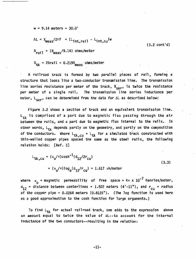
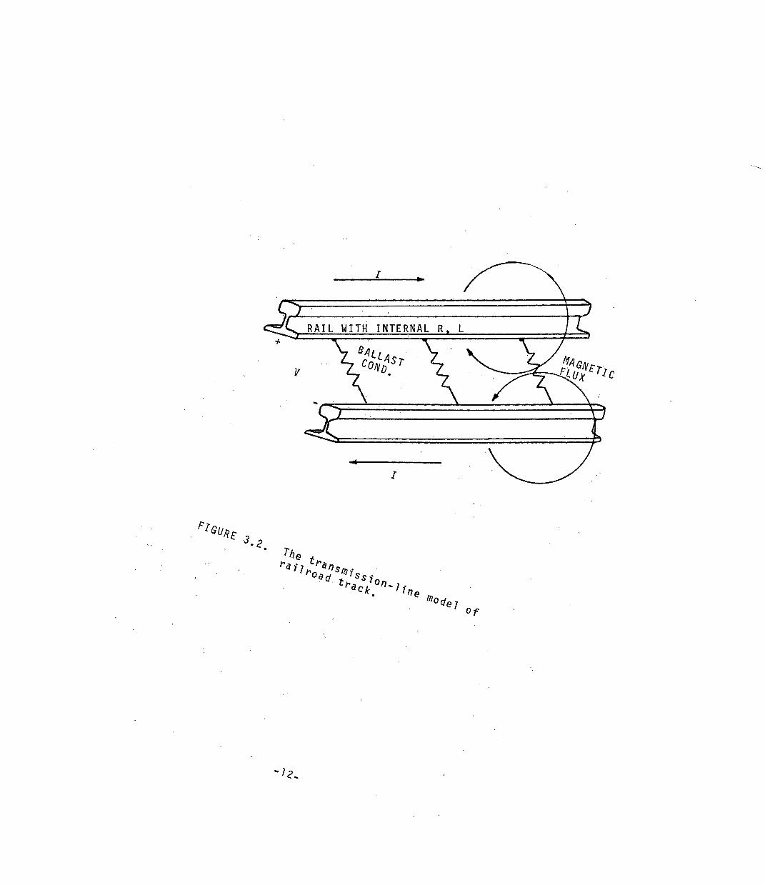
Figure 3.2 shows a section of track and an equivalent transmission line. I_tk is comprised of a part due to magnetic flux passing through the air between the rails, and a part due to magnetic flux internal to the rails. In other words, l_tk depends partly on the geometry, and partly on the composition of the conductors. Where cu = Ltk for a simulated track constructed with thin-walled copper pipes spaced the same as the steel rails, the following relation holds: [Ref. 3]

-1/Ltk,cu * ( V ’)<:osh' ‘V ^ c u 1= (ll0/ir)lo9e(d12/rcu) = 1.617 uh/meter

(3.3)

where uq = magnetic permeability of free space = 4* x 10” henries/meter, d12 = dlstance between centerlines - 1.502 meters (4'-H"), and rcu = radius of the copper pipe = 0.0264 meters (0.8125"). (The log function is used here as a good approximation to the cosh function for large arguments.)

To find Ltk for actual railroad track, one adds to the expression above an amount equal to twice the value of AL--to account for the internal inductance of the two conductors— resulting in the relation:

-11-

/ *>

rieu

*

t c kn'if Oq®0dte; O f

Je*

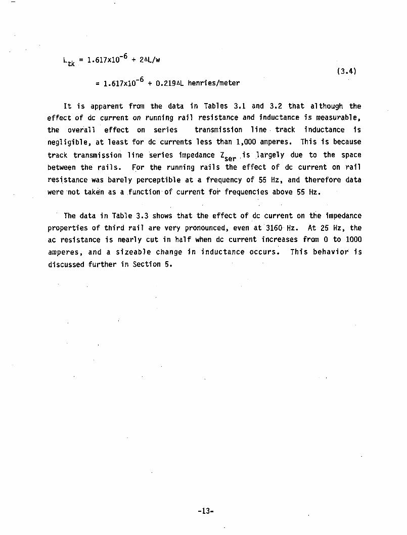
= 1.617xl0~6 + 0.219AL henries/meter

Ltk = 1.617X10"6 + 2AL/w(3.4)

It is apparent from the data in Tables 3.1 and 3.2 that although the effect of dc current on running rail resistance and inductance is measurable, the overall effect on series transmission line track inductance is negligible, at least for dc currents less than 1,000 amperes. This is because track transmission line series impedance Zser is largely due to the space between the rails. For the running rails the effect of dc current on rail resistance was barely perceptible at a frequency of 55 Hz, and therefore data were not taken as a function of current for frequencies above 55 Hz.

The data in Table 3.3 shows that the effect of dc current on the impedance properties of third rail are very pronounced, even at 3160 Hz. At 25 Hz, the ac resistance is nearly cut in half when dc current increases from 0 to 1000 amperes, and a sizeable change in inductance occurs. This behavior is discussed further in Section 5.

-13-

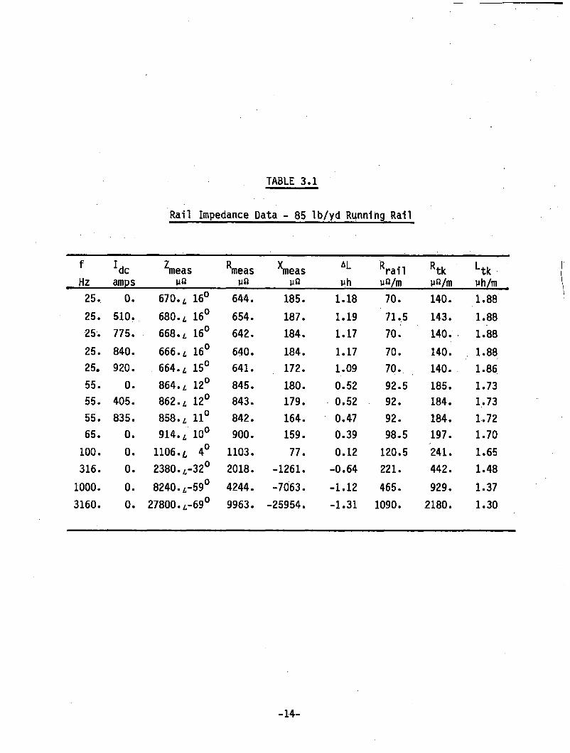
TABLE 3.1

Rail Impedance Data - 85 Ib/yd Running Rail

fHz amps ^measyfl ^easyfl ^neasyn

A L yh Rrailyfl/m Rtkyn/m Ltkyh/m

25. 0. 670.L 16° 644. 185. 1.18 70. 140. 1.8825. 510. 680.L 16° 654. 187. 1.19 71.5 143. 1.8825. 775. 668.i 16° 642. 184. 1.17 70. 140. 1.8825. 840. 666.L 16° 640. 184. 1.17 70. 140. 1.8825. 920. 664. 15° 641. 172. 1.09 70. 140. 1.8655. 0. 864.i 12° 845. 180. 0.52 92.5 185. 1.7355. 405. 862.L 12° 843. 179. 0.52 92. 184. 1.7355. 835. 858.i 11° 842. 164. 0.47 92. 184. 1.7265. 0. 914.L 10° 900. 159. 0.39 98.5 197. 1.70100. 0. 1106.L 4° 1103. 77. 0.12 120.5 241. 1.65316. 0. 2380.^-32° 2018. -1261. -0.64 221. 442. 1.481000. 0. 8240.^-59° 4244. -7063. -1.12 465. 929. 1.373160. 0. 27800.^-69° 9963. -25954. -1.31 1090. 2180. 1.30

-14-

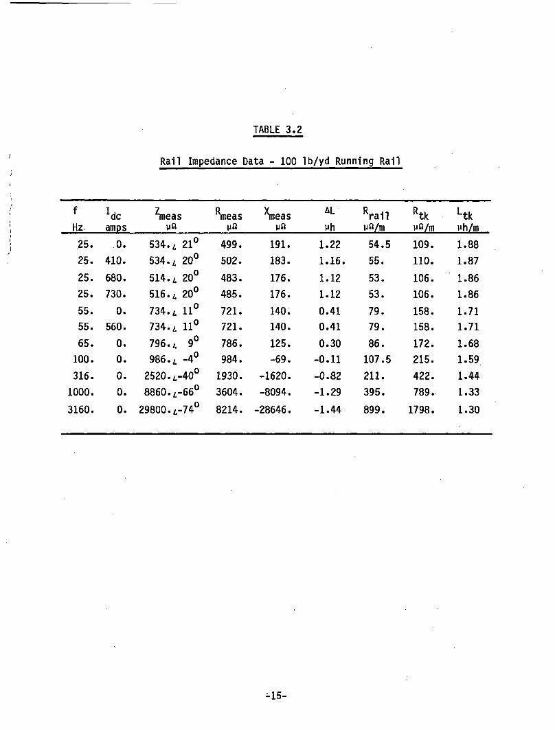
TABLE 3.2

Rail Impedance Data - 100 Ib/yd Running Rail

fHz. ■dcamps ^easyn ^neasy«

Ymeasy«ALyh Rrail

yn/m Rtkyfl/m Ltkyh/m25. 0. 534. 21° 499. 191. 1.22 54.5 109. 1.8825. 410. 534.l 20° 502. 183. 1.16. 55. 110. 1.8725. 680. 514./; 20° 483. 176. 1.12 53. 106. 1.8625. 730. 516.L 20° 485. 176. 1.12 53. 106. 1.8655. 0. 734.L 11° 721. 140. 0.41 79. 158. 1.7155. 560. 734.L 11° 721. 140. 0.41 79. 158. 1.7165. 0. 796.L 9° 786. 125. 0.30 86. 172. 1.68100. 0 . 986./, -4° 984. -69. -0.11 107.5 215. 1.59316. 0 . 2520./.-400 1930. -1620. -0.82 211. 422. 1.441000. 0. 8860. z,-66° 3604. -8094. -1.29 395. 789. 1.333160. 0. 29800.^-74° 8214. -28646. -1.44 899. 1798. 1.30

-15-

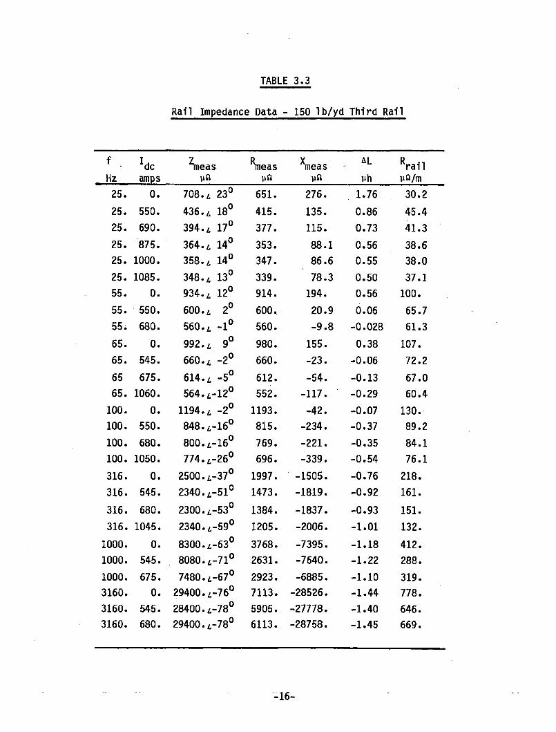
TABLE 3.3

Rail Impedance Data - 150 Ib/yd Third Rail

fHz

■dcamps

Zmeasyn ^easyn ^neasy«ALyh

Rrailya/m

25. 0. 708.L 23° 651. 276. 1.76 30.225. 550. 436.L 18° 415. 135. 0.86 45.425. 690. 394. 17° 377. 115. 0.73 41.325. 875. 364.L 14° 353. 88.1 0.56 38.625. 1000. 358.L 14° 347. 86.6 0.55 38.025. 1085. 348.L 13° 339. 78.3 0.50 37.155. 0. 934.L 12° 914. 194. 0.56 100.55. 550. 600.L 2° 600. 20.9 0.06 65.755. 680. 560.L -1° 560. -9.8 -0.028 61.365. 0. 992.L 9° 980. 155. 0.38 107.65. 545. 660.L -2° 660. -23. -0.06 72.265 675. 614.L -5° 612. -54. -0.13 67.065. 1060. 564.£-12° 552. -117. -0.29 60.4100. 0. 1194.L -2° 1193. -42. -0.07 130.100. 550. 848.£-16° 815. -234. -0.37 89.2100. 680. 800. *.-16° 769. -221. -0.35 84.1100. 1050. 774.A-26° 696. -339. -0.54 76.1316. 0. 2500./.-370 1997. -1505. -0.76 218.316. 545. 2340.£-51° 1473. -1819. -0.92 161.316. 680. 2300.£-53° 1384. -1837. -0.93 151.316. 1045. 2340.£-59° 1205. -2006. -1.01 132.1000. 0. 8300.£-63° 3768. -7395. -1.18 412.1000. 545. 8080.£-71° 2631. -7640. -1.22 288.1000. 675. 7480. *,-67° 2923. -6885. -1.10 319.3160. 0. 29400.£-76° 7113. -28526. -1.44 778.3160. 545. 28400.£-78° 5905. -27778. -1.40 646.3160. 680. 29400.£-78° 6113. -28758. -1.45 669.

-16-

4. COMPARISON OF CALCULATED AND MEASURED TRACK IMPEDANCE

The track series resistance and inductance calculated in Section 3 on the basis of measured rail properties agree very closely with results of measurements of series impedance of actual track. The track on which measurements were made had 115 lb/yard rail, and thus was slightly larger in crossectional area than the 100 lb/yard rail used in rail impedance tests. However, since perimeter varies as (area)*/2, the perimeter of the 115 lb/yard rail was only an estimated 1% larger than that of the 100 lb/yard rail.

Measurements of series track impedance of a length of rapid transit track 213 meters (700‘) long were made. The track was composed of 115 Ib/yd running rail on wooden ties on crushed aggregate ballast. The the running rails were shorted at one end, and an audio-frequency signal source was connected to the open end. An oscilloscope was used to measure relative amplitudes and phases of current and voltage waveforms, at a number of specific frequencies, and the short-circuit input impedance Z was determined at each of these frequencies.

Ballast resistance was unknown, and was not measured. However, the ballast was "clean," since the track was part of a little-used siding, and it is estimated that ballast resistance was in excess of 15,000 ohm-meters (49.2 ohm-kft, i.e., 49.2 "ohms in a thousand feet"). To assess our ability to infer series track impedance from measurement of Zsc, we briefly must review transmission line theory [Ref. 4].

Railroad track essentially is a transmission line. A transmission line is characterized by series impedance Zger per unit length and shunt admittance Ysf1 per unit length. These parameters determine the transmission line's propagation coefficient and characteristic impedance:

y = <zserYsh)1/2 = a + je per meter

zo - (zser/vsh>1/2 ohms(4.1)

-17-

Current and voltage waves travel along a transmission line with spatial variation given by

V+{z,w) = A exp(-yz)

I+(z,<») = V+(z,<*))/ZQ(4.2)

V (z.u) = B exp(+Yz)

I_(z,u)) = -V_(z,to)/Z0

The "+" and subscripts denote waves travelling in the +z and -z directions respectively. The propagation coefficient y = a + je gives the spatial rates of attenuation and phase shift of waves on the transmission line. For lossless transmission lines, a = 0, and y is purely imaginary. In the case of railroad track', non-zero rail resistance and non-infinite ballast resistance both cause a to be non-zero. Figure 4.1 depicts waves travelling in the +z and -z directions.

Treating the track as a transmission line, with series impedance Z .. =I £ v l \

Rser tk + jXser tk ohms meter of length, and shunt conductance Y$h tk = d/Rballast) mhos/meter of length, the propogation coefficient y for the track is

Zser,tk^Rballast^ 1/2 (4.3)

For shorted sections of track with length d sufficiently short, i.e., for Iy Id << 1, the shorted section of track will have an input impedance Zsc approximately equal to Zser tkd. However, the approximation starts breaking down for values of I Yd I much larger than 0.1. In other words, when conduction from one rail to the other through the ballast becomes almost as easy as conduction clear down one rail, across the short, and back, you can no longer measure the impedance of the rail loop accurately from one end, because you will be looking also at some ballast shunting it.

-18-

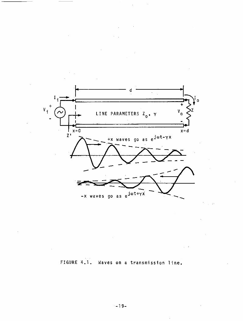
FIGURE 4.1. Waves on a transmission line.

- 1 9 -

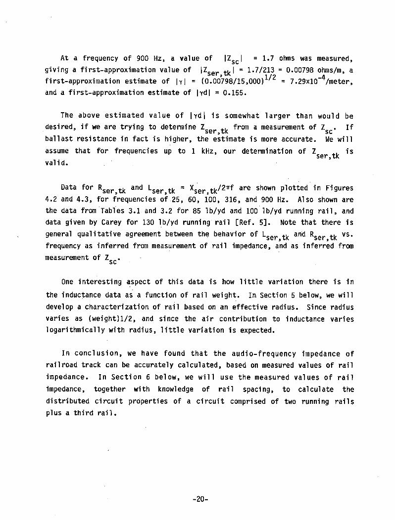
At a frequency of 900 Hz, a value of |Z | = 1.7 ohms was measured,giving a first-approximation value of \lcav. +lr | = 1.7/213 = 0.00798 ohms/m, aser,wc i /o afirst-approximation estimate of |y| = (0.00798/15,000) = 7.29x10 /meter,and a first-approximation estimate of |yd| = 0.155.

The above estimated value of |yd| is somewhat larger than would bedesired, if we are trying to determine Z .. from a measurement of Z . IfseryvK scballast resistance in fact is higher, the estimate is more accurate. We will assume that for frequencies up to 1 kHz, our determination of Z is

S 6 T f tKvalid.

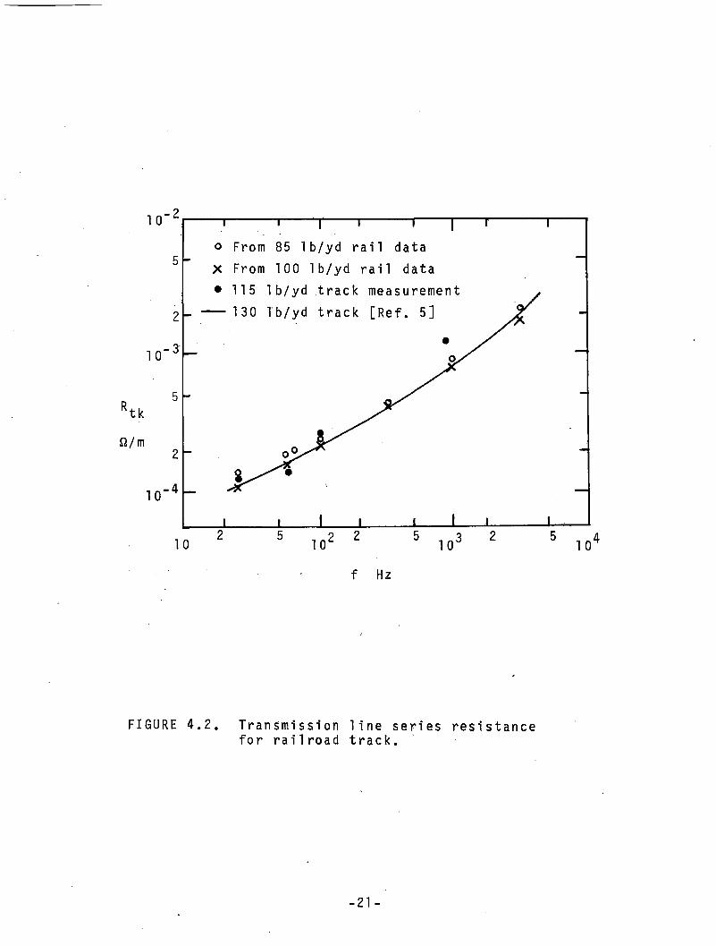
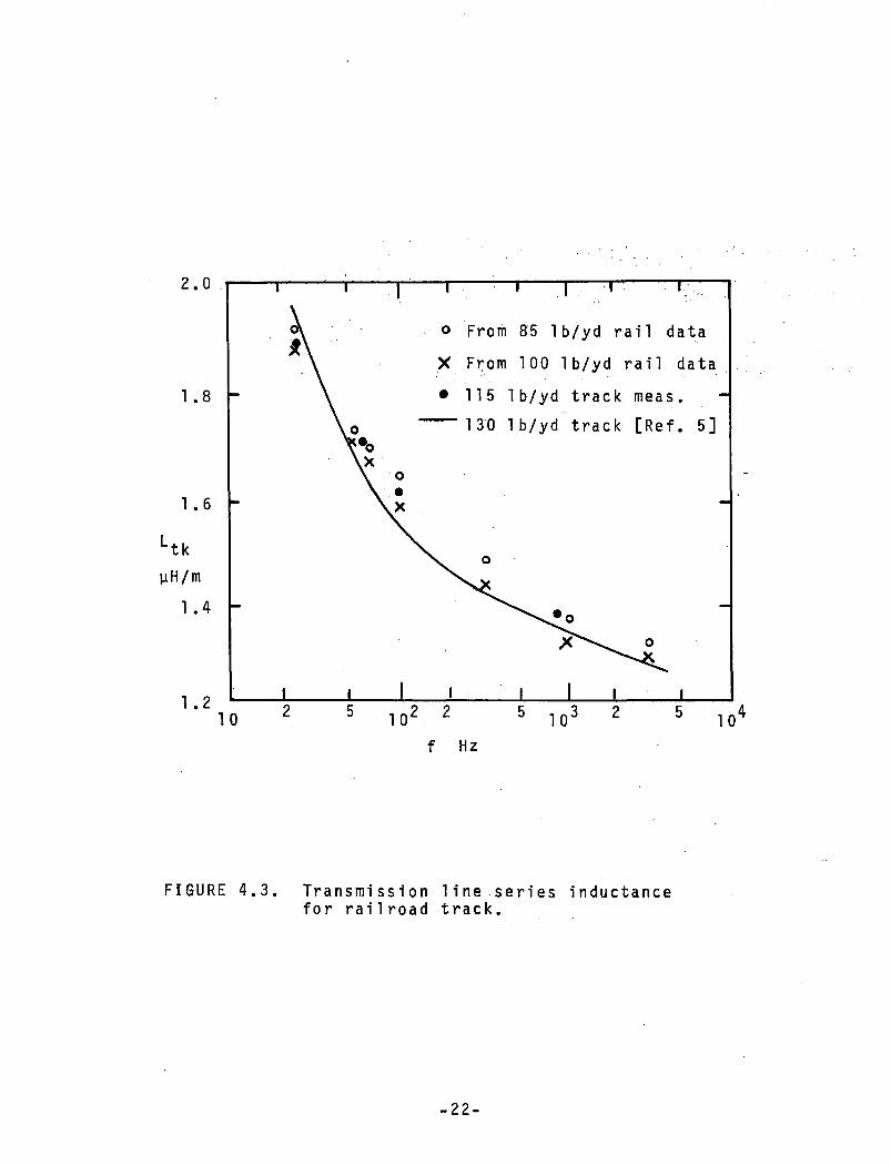
Data for Rger and Lser tk = Xser tk/2"f are shown plotted in Figures4.2 and 4.3, for frequencies of 25, 60, 100, 316, and 900 Hz. Also shown arethe data from Tables 3.1 and 3.2 for 85 Ib/yd and 100 Ib/yd running rail, anddata given by Carey for 130 lb/yd running rail [Ref. 5]. Note that there isgeneral qualitative agreement between the behavior of Lser tk and R$er tk vs.frequency as inferred from measurement of rail impedance, and as inferred frommeasurement of Z .sc

One interesting aspect of this data is how little variation there is in the inductance data as a function of rail weight. In Section 5 below, we will develop a characterization of rail based on an effective radius. Since radius varies as (weight)1/2, and since the air contribution to inductance varies logarithmically with radius, little variation is expected.

In conclusion, we have found that the audio-frequency impedance of railroad track can be accurately calculated, based on measured values of rail impedance. In Section 6 below, we will use the measured values of rail impedance, together with knowledge of rail spacing, to calculate the distributed circuit properties of a circuit comprised of two running rails plus a third rail.

-20-

n/m

10 2 2

f Hz

FIGURE 4.2. Transmission line series resistance for railroad track.

-21 -

f Hz

FIGURE 4.3. Transmission line series inductance for railroad track.

-22-

5. MEASURED RAIL IMPEDANCE VS. SKIN EFFECT THEORY [Ref. 6]

5.1 Skin Effect Theory - the Skin Depth Parameter

It would be desirable to have a simple model that accounted for rail impedance as a function of frequency. For non-ferrous conductors of regular geometry, such models do exist. They take into account the magnetic permeability, dielectric constant, and conductivity of the conducting medium. For planar conductors, solutions for surface impedance involve exponential functions, as is discussed below. For circular conductors, solutions involve Bessel functions; but empirically, impedance behavior becomes very simply described at very high frequencies.

Railroad rail does not present such a simple case. It has very irregular crossection, and it is made from ferrous material. We believe that a complete accounting of high-frequency impedance of steel rails must take magnetic hysteresis into account, probably by ascribing an imaginary part to the magnetic permeability. Such an effort is beyond the scope of this project. What follows is a description of the Skin Effect, and its application to steel rails in a qualitative manner.

At high frequencies, electromagnetic fields are excluded from the interior of good conductors, and ac currents only flow on the surface of the conductors. This phenomenon is referred to as the Skin Effect. Current density decreases exponentially with depth below the surface of a conductor with plane surface. The skin depth parameter 6 is equal to the inverse of the real part of the propagation coefficient for electromagnetic waves within the conductor. The propagation coefficient y is given by the relation

Y = a + js = [(juniMa + jwe)]^^ (5.1)

In a metallic conductor at frequencies less than 1016 Hz, a » we and the resulting relations for y, <*> and & are

-23-

Y = (1 + j ) (irf vicr)1/2

a = 3 = Re[y] = (irfua)^2 (5.2.)

6 = 1/ a = ( i r f j i a )

where u = magnetic permeability and o = conductivity of the conductor.

5.2 Skin Effect in Conductors of Circular Crossection

For a solid conductor of circular crossection, variation of current density with depth is given by Bessel functions of complex argument. However, at high frequencies, where s becomes much less than the radius of the conductor, decrease in current density vs. depth once again becomes exponential. For conductors of irregular crossection such as railroad rails, only numerical solutions for current distribution exist. However, beginning at a specific point on the surface of the conductor, as frequency increases and skin depth becomes much less than the radius of curvature of the surface, current once again will decrease exponentially as a function of depth.

As frequency increases and the effective current-carrying crossection of a conductor decreases, the series impedance per unit length increases. The series resistance and internal reactance, which is that part of reactance due to fields within the conductor, each increase with increasing frequency.

One surprising aspect of the skin effect phenomenon is that in a non- ferrous solid circular conductor at high frequencies, the internal reactance becomes equal to the series resistance. This fact can be understood by examining the behavior of electromagnetic fields beneath the surface of a plane conductor at high frequencies. The characteristic impedance for plane waves within a conducting medium is

ZQ = [ j o ) u / ( o + ju>e) ] 1 / 2 ( 5 . 3 )

In a metal laic conductor, at frequencies below 1016 Hz, the resulting form of Zo is

-24-

(5.4)ZQ = ( 1 + j ) U f w/ a ) 1 / 2

Since the real and imaginary parts of ZQ are equal, sheet current just beneath the surface of the conductor will give rise to exactly equal resistive and reactive components of electric field at the surface of the conductor. Thus, the resistive and reactive components of "internal impedance," due to fields and currents within the conducting medium, are equal.

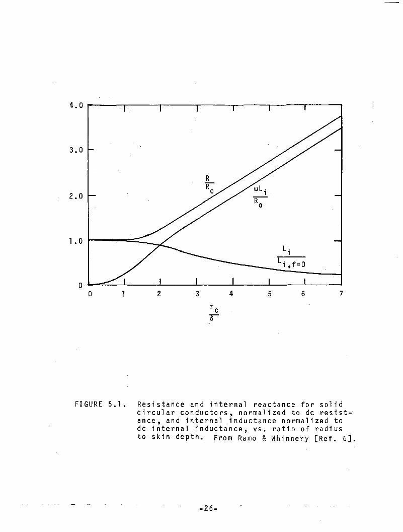
Figure 5.1 shows behavior of resistance, internal reactance, and internalinductance per unit length for a non-ferrous circular conductor as a functionof (r /<s), where r is the conductor radius. Note that values of resistance c cand reactance are normalized to the low-frequency resistance per meter

R0 = l/oirrc2 (5.5)

Note that (r /«) is proportional to f1^2. For (r_/6) > 2, very good approximation's for resistance, internal reactance, and internal inductance are:

R/R0 = 0.25 + rc/2«

R = 0.25Rq + R0rc/26

= 0.25R + (u/a)1/2(l/2TT1/2r )f1/2 (5.6)U U

xint “ “Lint “ Rorc/25Lint - > r " 2

The above relations show that as far as causing a large value of t is concerned, a large value of u has no more effect than a small value of o. This surprising result is somewhat at odds with intuition, but it is a direct result of the propagation characteristics of electromagnetic waves penetrating the surface of the conductor, as discussed above.

-25-

6

FIGURE 5.1. Resistance and internal reactance for solidcircular conductors* normalized to dc resistance, and internal inductance normalized to dc internal inductance, vs. ratio of radius to skin depth. From Ramo & Whinnery [Ref. 6]

2 6 -

5.3 Skin Effect in Railroad Rail

It is not possible to construct a model for railroad rails based on equivalent non-ferrous conductors of circular crossection that accurately accounts for both internal rail inductance and resistance. The behavior prescribed for such a model in Eqn. 5.6 specifies very rigorously the relation between R, xint* ®nd Lint* as a functlon of frequency. Analysis of data for the rails tested shows that the behavior of the impedance parameters as a function of frequency does not conform to such a model. One reason is that magnetichysteresis loss leads to higher skin resistance; inclusion of hysteresis effects is beyond the scope of this report. However, such a model can account for the behavior of rail inductance alone as a function of frequency. Such a model is useful at audio frequencies, where the preponderant part of overall track impedance is the inductive part, and where the preponderant part of the inductance is due to the free space between the rails. The relation of measured rail data to equivalent circular models is presented here.

Based on nominal data provided by Frielinghaus [Ref. 7], for conductivity and permeability of steel running rail, namely

a ... - o /12.1 = 4.79x10® mhos per meter rail cu K (5.7)yrail = 20yo = 20x4irXl°7 = 2.51x10“5 henries/meter

the nominal value of skin depth at 25 Hz is 1 cm. This distance is much less than the radius of a circle whose area equals the crossection of railroad rail. However, it is approximately equal to the thickness of the web or lower flange.

We can determine a value of effective radius from measured inductance vs. frequency. From Eqn. 5.6, the expected form for measured rail inductance per meter as described in Section 3 is

L,meas = ( V 2ir)1°9e(rcu/r«ev cu' eff (5.8)+ (ji ../arail rail

-27-

where reff is the radius of equivalent circular conductor, and rcu is the radius of the copper pipe that served as a reference.

In Eqn. 5.8, it is seen that as f ® and f-1/2 -*■ o, thefrequeny-dependent term disappears, leaving a term dependent only on r and

1 / 9r^,.. A plot of L vs. f ' for the 100 lb/yd running rail is shown inFigure 5.2. A best-fit straight line drawn through the data points yields an intercept at f"1/2 = o of -1.65 uh, or 1.65/9.14 = -0.1805 uh/meter, and a corresponding effective radius of

reff = rcuexp(0.1805uo/2ir) = 5.09 cm = 2 inches (5.9)

The slope of the line is 14.5 uh Hz*^, which divided by the 9.14 meter length yields a slope of 1.59 uh m"* H z ^ . Taking the value of rgff from Eqn. 5.9 and the value of this slope, and using Eqn. 5.8 to solve for an effective value of (u/<0 based on this inductance data, we obtain

(u/a) = 16*3r2ff(1.59 x 10“6)2 = 3.23 x 10-12 ohm-henries (5.10)

This value of (u/a), together with the effective radius, can be used to calculate rail internal inductance and track inductance over the range of frequencies covered with very good accuracy. Of course, the accuracy is enhanced by the fact that as far as the inductance of two-rail track is concerned, the preponderance of the inductance is due to the free space between the rails.

Note that we have no way to separately determine u ... or <* ... from ourdata, since all our data was taken at frequencies at which skin depth was manytimes less than ref . The value determined here is in qualitative agreement,but significantly different from the corresponding value calculated from the1 ?data given in Eqn. 5.7 of 5.24 x 10 ohm-henries.

The impedance properties of the 150 lb/yd third rail show striking variation over a dc current range from 0 to 1000 amperes. The data from Table3.3 have been used to construct plots of Lmeas as a function of f^/2 f0r the

-28-

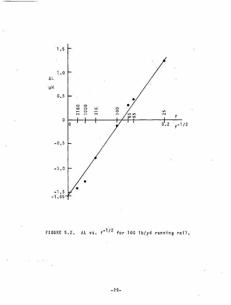
FIGURE 5.2. AL vs. for 100 lb/yd running rail.

-29-

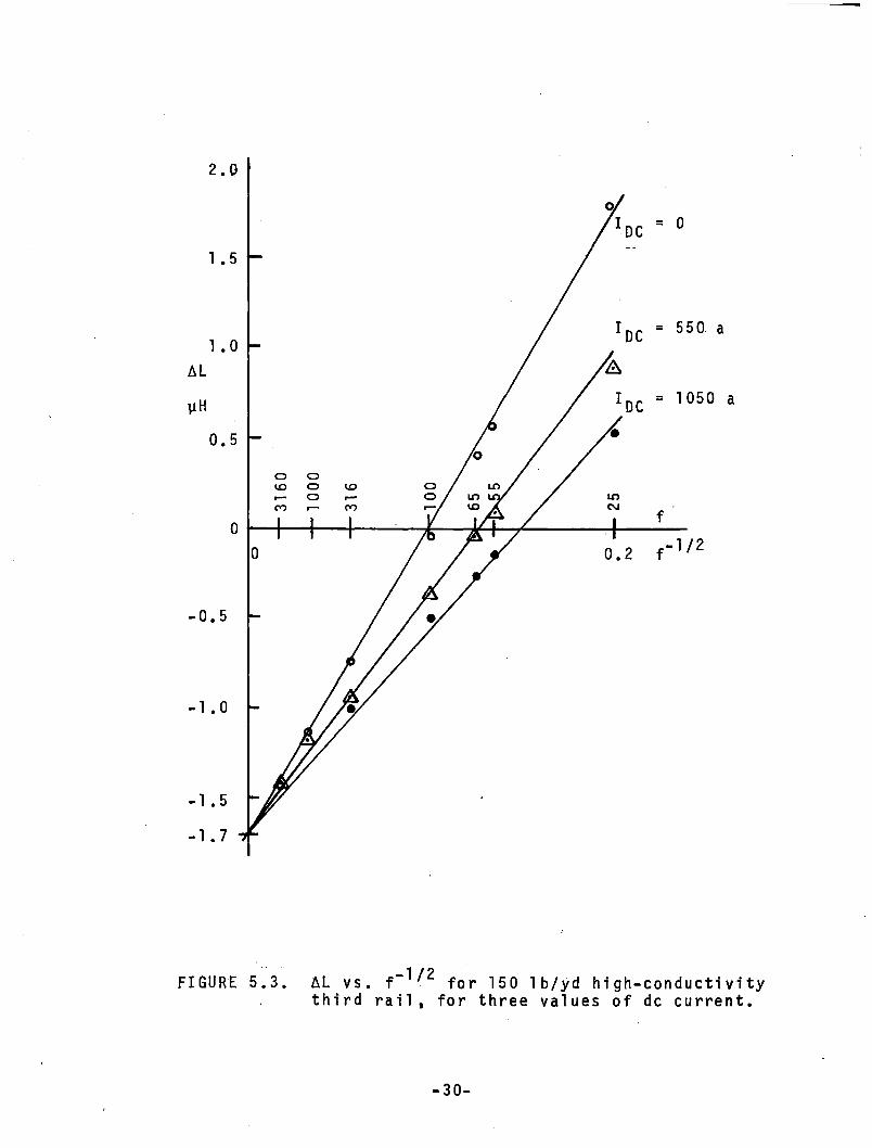
2.0

FIGURE 5.3. AL vs. f“V ^ for 150 1 b/yd high-conductivity third rail, for three values of dc current.

- 3 0 -

third rail, for dc currents of 0, 550 amperes, and 1050 amperes. These plots are shown in Figure 5.3. A family of straight lines has been drawn, one for each value of ld , with a common vertical-axis intercept, and with a qualitatively good fit to the corresponding data points.

The lines intersect the vertical axis at -1.7 uh, or -0.1860 uh/meter for the 9.14 meter length, and the lines have slopes of 1.89 x 10~®, 1.40 x 10“®, and 1.22 x 10”® h'nf^Hz^, for the corresponding dc currents of 0, 550, and 1050 amperes.

The value of -0.1860 uh/m yields an effective radius for the third rail of

reff = rcuexP(0*1860uo/2") = 5.23 cm (5.11)

Using the three values of slope above in place of the 1.59 x 10"® value in Eqn. 5.10, and using the new value of rg , we obtain the following estimates of (m/0) for the three currents:

We can assume that the value of ° remains the same, but that the effective small-signal value of u decreases as dc magnetic field saturates the metal near the surface of the rail. The drop in v with increasing dc current leads to an increase in skin depth, and a corresponding decrease in rail resistance as seen in the data of Table 3.3.

The drop in the internal inductance of the third rail seen here is large enough to be significant as far as conductive interference is concerned. In Section 6, we will see that the total inductance of the third-rail running- rail loop is has a nominal value based on air inductance of 0 .9 uh/meter of circuit length. At 25 Hz, we see a decrease here of 0.135 yh/meter in third

Idc, amps u/°, ohm-henries for 150 lb/yd third rail

5501050

0 4.85 x 10" 1 2

2 .66 x 1 0 " 12

2 .0 2 x 1 0 “ 12

rail internal inductance, and therefore a corresponding decrease in the third-rail running rail loop inductance, as current increases from 0 to 1050 amperes.

This variation in y with current also is an indication that the third rail could be a significant factor in producing harmonics and intermodulation products of interference signals present at chopper and substation harmonic frequencies. We do not know how significant the third rail is at causing such mixing in comparison with other nonlinear elements in the system, but we can see that the running rails will be practically free of such effects in comparison to third rail such as that tested here.

5.4 Conclusions

Railroad running rail of a variety of weights is seen to have internal inductance properties equivalent to solid steel circular cylinders of radius 5.09 cm (2"), with a ratio (y/a) equal to 3.23 x 10"12 ohm-henries. Since air inductance is the dominating term in the series transmission line impedance of railroad track, a model for total track inductance based on these properties gives accurate results, and magnetic hysteresis effects can be neglected.

Third rail of an alloy with a high copper content was found to have internal inductance properties that varied significantly with dc current. The 150 Ib/yd rail tested had inductance properties equivalent to a solid cylinder of radius 5.23 cm (2.06"), and an effective small-signal magnetic permeability that decreased with increasing dc current.

As will be seen in Sections 6.9 - 6.11, the internal inductance of the third rail directly enters the expressions for series impedance of the third- rail running-rail loop. At 25 or 60 Hz, the loop inductance per meter will decrease by almost 0 . 1 yh/meter as current through the third rail tested increases from 0 to 1,000 amperes. And, we cannot say, based on the data taken, how much the decrease would be as the dc third-rail current increased to 10,000 amperes. However, since this loop inductance is dominated by air inductance, this variation should not be of actual concern, especially at audio frequencies where variation is less.

-32-

6. CIRCUIT ANALYSIS OF TRACK WITH THIRD RAIL, TRACK CIRCUITS, AND BALLAST

6.1 The Model

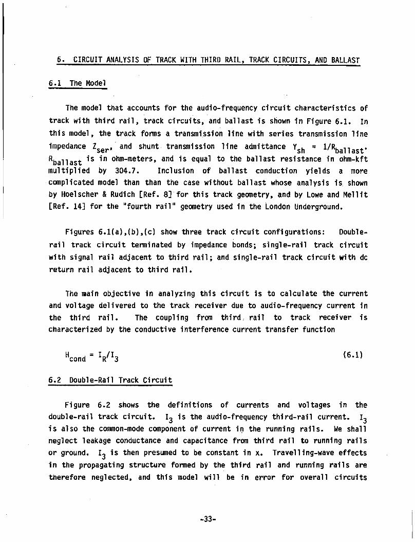
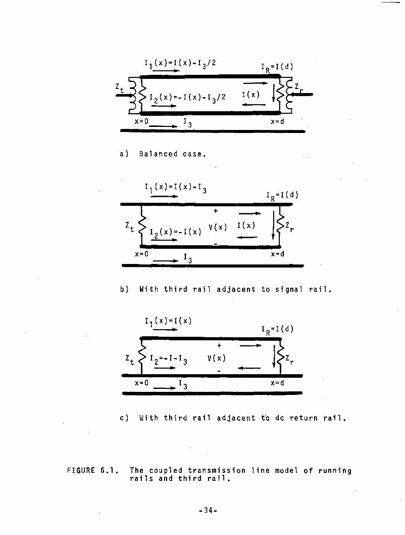
The model that accounts for the audio-frequency circuit characteristics of track with third rail, track circuits, and ballast is shown in Figure 6.1. In this model, the track forms a transmission line with series transmission line impedance Z$er, and shunt transmission line admittance Y$h = 1/Rban asf Rballast ls in ohm_meters» and 1S equal to the ballast resistance in ohm-kft multiplied by 304.7. Inclusion of ballast conduction yields a more complicated model than than the case without ballast whose analysis is shown by Hoelscher & Rudich [Ref. 8] for this track geometry, and by Lowe and Mellit [Ref. 14] for the "fourth rail" geometry used in the London Underground.

Figures 6.1(a),(b),(c) show three track circuit configurations: Doublerail track circuit terminated by impedance bonds; single-rail track circuit with signal rail adjacent to third rail; and single-rail track circuit with dc return rail adjacent to third rail.

The main objective in analyzing this circuit is to calculate the current and voltage delivered to the track receiver due to audio-frequency current in the third rail. The coupling from third rail to track receiver is characterized by the conductive interference current transfer function

Hcond V*36.2 Double-Rail Track Circuit

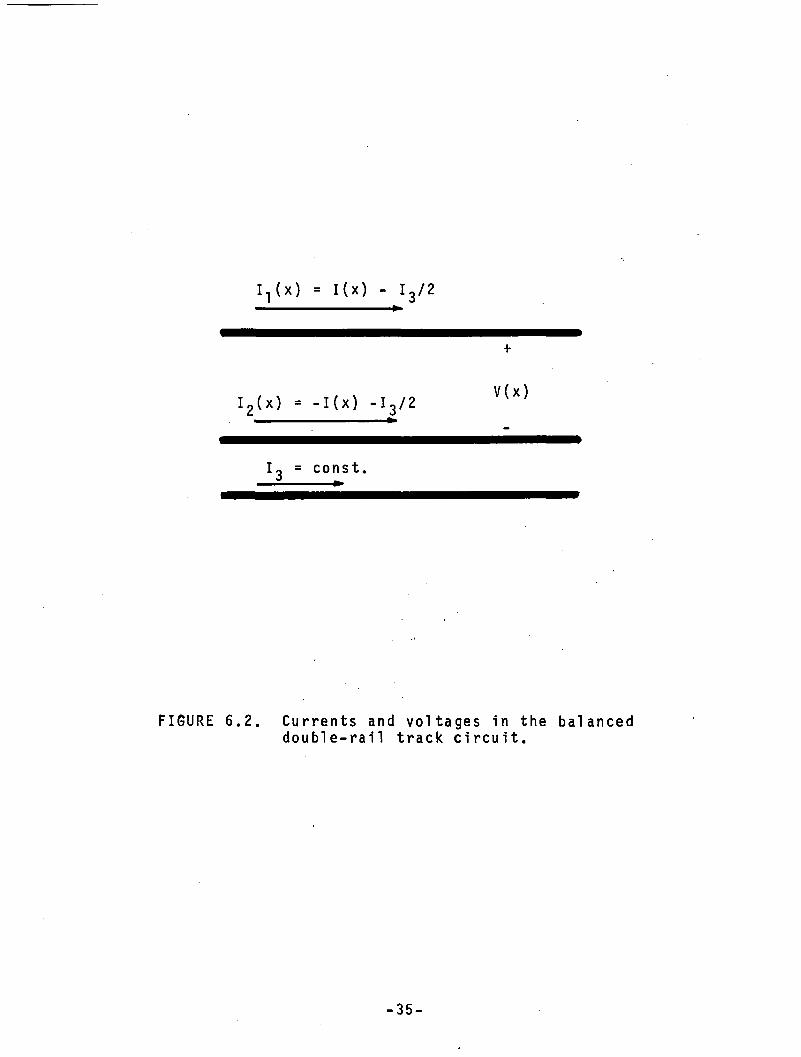
(6.1)

Figure 6.2 shows the definitions of currents and voltages in the double-rail track circuit. Ig is the audio-frequency third-rail current. ig is also the common-mode component of current in the running rails. We shall neglect leakage conductance and capacitance from third rail to running rails or ground. Ig is then presumed to be constant in x. Travelling-wave effects in the propagating structure formed by the third rail and running rails are therefore neglected, and this model will be in error for overall circuits

-33-

^ ( x )=I(x )-I3/2h mi M

a) Balanced case.

(x)=I(x)-I3

1 I2 (x)=-I(x) V (x)

x = 0

h mlM

x = d

b) With third rail adjacent to signal rail.

I -i C x) = I (x )--- ► IR=I(d)

x=0 I- x=d■ * O

c) With third rail adjacent to dc return rail.

FIGURE 6.1. The coupled transmission line model of running rai 1 s and third rai1 .

-34-

+

I2 (x) = -I(x) -I3 / 2V (x)

I3 = const.

FIGURE 6.2. Currents and voltages in the balanced double-rail track circuit.

-35-

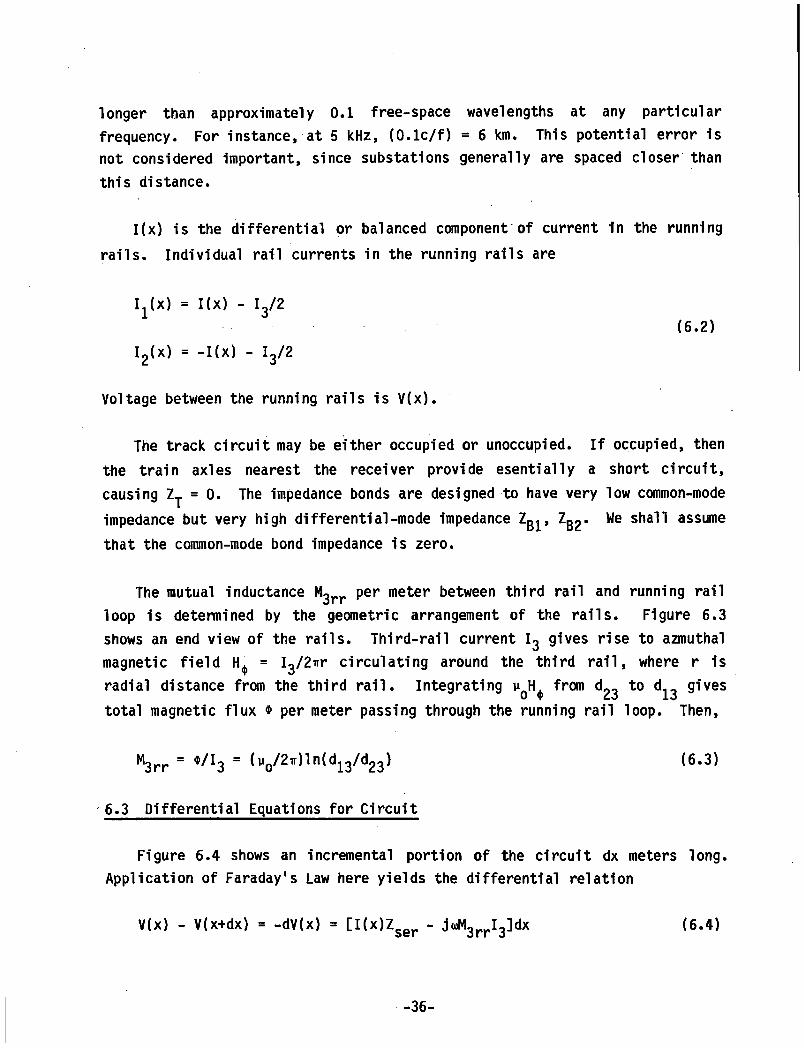
longer than approximately 0 . 1 free-space wavelengths at any particular frequency. For instance, at 5 kHz, (O.lc/f) = 6 km. This potential error is not considered important, since substations generally are spaced closer than this distance.

I(x) is the differential or balanced component of current In the running rails. Individual rail currents in the running rails are

Ix(x) = I(x) - I3 /2

(6.2)I2(x) = -I(x) - I3/2

Voltage between the running rails is V(x).

The track circuit may be either occupied or unoccupied. If occupied, then the train axles nearest the receiver provide esentially a short circuit, causing = 0. The impedance bonds are designed to have very low common-modeimpedance but very high differential-mode impedance ZB2. We shall assume that the common-mode bond impedance is zero.

The mutual inductance M3rr per meter between third rail and running rail loop is determined by the geometric arrangement of the rails. Figure 6.3 shows an end view of the rails. Third-rail current I3 gives rise to azmuthal magnetic field = I3/2irr circulating around the third rail, where r is radial distance from the third rail. Integrating from d23 to d1 3 gives total magnetic flux * per meter passing through the running rail loop. Then,

M3rr = */!3 = (6.3)

6.3 Differential Equations for Circuit

Figure 6.4 shows an incremental portion of the circuit dx meters long. Application of Faraday's Law here yields the differential relation

V(x) - V(x+dx) = -dV(x) = [I(x)Zser - j«M3rTI3]dx (6.4)

-36-

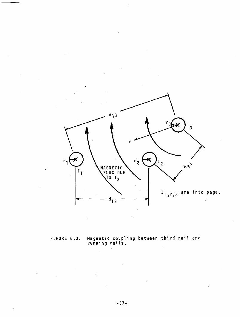
FIGURE 6.3. Magnetic coupling between third rail and running rails.

-37-

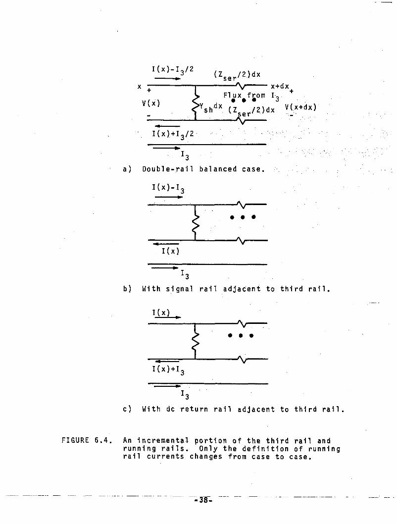
FIGURE 6.

U xM 3 / 2 (Zser/2.Jdx+V(x)

A r x+dxFlux fjjom I-g •

>Yshdx (Z er/?.)dx v(x+dx^ — — — \ ----

I (x ) + 1 3 / 2

a) Double-rail balanced case. I(x)-I3

— A / -----• • •

I(x)Ar

b) With signal rail adjacent to third rail

I(x)At

• •

I(x)+I3A r

c) With dc return rail adjacent to third rail

. An incremental portion of the third rail and running rails. Only the definition of running rail currents changes from case to case.

which translates into the differential equation

dV(x)/dx = -I(x)Zser + jo>M3rrI3 (6.5)

The corresponding differential relation for current is

I(x) - I(x+dx) = -dl(x) = YshV(x) (6.6)

which yields the differential equation

dl(x)/dx = -YshV(x) (6.7)

Differentiating Eqn. 6.5 once again while remembering that dl3/dx = 0, and substituting in the relation for dl/dx from Eqn. 6.7, we obtain the second-order differential equation

d2V(x)/dx2 = YshZ$erV(x) (6.8)

Where the complex propagation parameter is

* ■ <YshZ« r ) 1/2 <6-9'

we can write a general solution for V(x) in terms of a weighted sum of rightward- and leftward-travel ling waves:

V(x) = Aexp(-fx) + Bexp(+yx) (6.10)

Differentiating Eqn. 6.10, substituting into Eqn. 6.5, and using the relation ZQ = zser/YSh 1/r2 91ves the relation for I(x):

I(x) = (l/ZQ)[Aexp(-Yx) - Bexp(+Yx)] + n 3/Zser)ja)M3rr (6.11)

-39-

6.4 An Equivalent Lumped Circuit

At this point we could solve any particular circuit with specific terminations at x = 0 and x = d by finding the values of A and B that match the boundary conditions for V(0)/I(0) and V(d)/I(d). We would then know V(x) and I(x) at every point in the circuit. This is more information than we need in most circumstances. What we really want to know are the values of current and voltage into the terminations at the ends of the circuit. Therefore, we will follow the approach outlined below of modelling the transmission-line structure by a simple lumped-circuit two-port network model that contains an internal voltage source to account for voltages induced by the third rail current.

The transmission line structure above is symmetrical end-for-end. It therefore can be modelled with an end-for-end symmetrical n-circuit as shown in Figure 6.5. To find the corresponding relations for Zj and Z2 in the equivalent n-circuit, we need only ask that the transmission line and the n-circuit both give equal input impedance Z. = V(0)/I(0) looking in at x = 0 for two cases: Output end open-circuited, i.e., 1(d) = 0; and output endshort-circuited, i.e., V(d) = 0. To find Z and Z2, we do this with I3 = 0. We will then let I3 be non-zero to find the proper form of V.. , which accounts for induced currents and voltages in the circuit due to I3.

Simultaneous solution of Eqn's 6.10, 6.11 for the short-circuit case gives

zisc = Cv(0)/I(0)]V(d)=0 = Zosinh(Yd)/cosh(Yd) = zll|z2 (6.12)where "||" is the "parallel" operator: Za||Zb = (Za~* + Zb“*)~*.

Simultaneous solution of Eqn's 6.10, 6.11 for the open-circuit case gives

Zioc = [V(0)/I(0)]I(d) . 0

= Z0cosh(Yd)/sinh(vd) = Z1 I|(Z1 + Z?)(6.13)

-40-

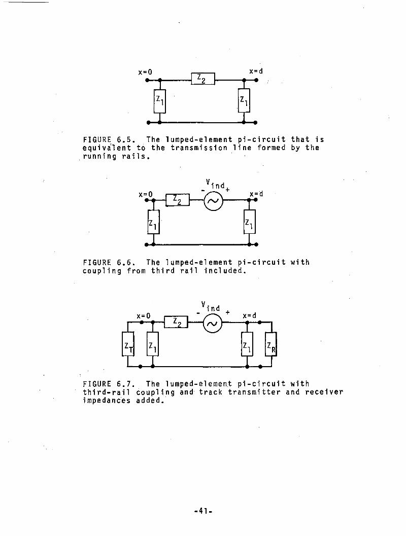
FIGURE 6.5. The lumped-element pi-circuit that is equivalent to the transmission line formed by the running rails.

FIGURE 6 .6 . The lumped-element pi-circuit with coupling from third rail included.

FIGURE 6.7. The lumped-element pi-circuit with third-rail coupling and track transmitter and receiver impedances added.

- 4 1 -

Then simultaneous solution of Eqns 6.12,13 gives

Z = Zosinh(Yd)/[cosh(Yd) - 1](6.14)

Z2 = ZQsinh(Yd)

The first step in finding the value of the induced voltage V.n<j shown in Figure 6.5 is to find the Thevenin-equivalent open-circuit output voltage Vth that appears at x = d when the track is shorted at x = 0 causing V(0) = 0. Figure 6 .6 shows the lumped circuit with Vth included. Setting V(0) = 0 in Eqn. 6.10 yields the relation B = -A for this case. Using this result to eliminate B from Eqn. 6.11, setting 1(d) = 0 in Eqn. 6.11, and solving the resulting relation for A yields

A = -B = -Igj M p/ZYCOShtYd) (6.15)

Examination of the circuit shown in Fig. 6 .6 and Eqn. 6.10 shows that

6.5 Single-Rail Track Circuits

In the single-rail track circuit with the signal rail adjacent to the third rail shown in Fig. 6.1(b), the signal current is noted as I(x). An analysis of an incremental portion of this circuit yields the differential relation

(6.16)

Using Eqn's 6.10,15,16 to solve for yields the result

vind = J“M3rrI3sinh(Yd)/Y (6.17)

V(x) - V(x+dx) = -dV(x) = [I(x)Zser - I3Zser./2 - j“M3rrI3]dx

" ™*>zser - + Zser/2)]dx

-42

(6.18)

Writing this as a differential equation, we have

dV(x)/dx = -I(x)Zser + I3 (j“M3rr + Zser/2) (6.19)

In the single-rail track circuit with the dc return rail adjacent to the third rail shown in Fig. 6.1(c), the signal current is also noted as I(x). An analysis of an incremental portion of this circuit yields the differential relation

V(x) - V(x+dx) = -dV(x) = [I{x)Zser + I3Zser/2 - j«M3n.I3]dx

“ n(x)Zser - I3 (j«M3rr - Z$er/2)]dx

The corresponding differential equation is

(6.20)

dV(x)/dx = -I(x)Zser + I3(j“M3rr - Zser/2) (6.21)

Equations 6.19 and 6.21 are the same as Eqn. 6.5, except that the tennjuM- in Eqn. 6.5 has been replaced with the term (juNL + Z /2) in the 3rr 3rr sercase where the signal rail is adjacent to the third rail, and by the term (j<DM3rr - zser/2 ) in the case where the dc return rail is adjacent to the third rail. These changes carry clear through an analysis similar to that covered in Eqn's 6.4-6.17 above, to yield these results for induced voltage in the lumped-element equivalent circuit for single-rail track circuits:

v1nd * l i M 3rr 1 Zser/2)I3sirh(,d)/T (6.22)

where ,,+“ is for the case where the signal rail is adjacent to the third rail, and is for the case where the dc return rail is adjacent to the third rail.

-43-

6 .6 Overall Result for Coupling from Third Rail

The following relation summarizes the effects of voltages induced in track circuits due to third-rail currents for the three types of circuits:

Vind = <>M3rr + kzser/2 )V ,nh(l,d)/l'k = 0 for balanced double-rail track circuit

k = + 1 for single-rail track circuit with signal rail (6.23)next to third rail

k = - 1 for single-rail track circuit with dc return rail next to third rail

6.7 The Conductive Interference Current Transfer Function

Figure 6.7 shows the lumped-element equivalent circuit with arbitrary transmitting-end and receiving-end impedances l j and ZR respectively. Direct analysis of this circuit shows that the current into the receiver IR is

JR = I(d> " W(6.24)

where Y1 = [ V (Zl + ZR)M(ZTI l ) + Z2 +■ (ZR| IZj)]

The current transfer function relating receiver current to third-rail current is then

Hcond = h n 3 * = Y'(j<oM3rr + kZser/2)s1nh(Yd)/Y (6.25)

For later use, at this time we will also define the corresponding transfer function relating induced transmitter current to I3:

Hcond * h ' h ’(6.26)

= {[Z1 /(Z1+ZT)]/[(ZTI|Z1 )+Z2+(ZRIlZ1 )]}(j«M3rr + kZser/2)sinh(Yd)/Y

-44-

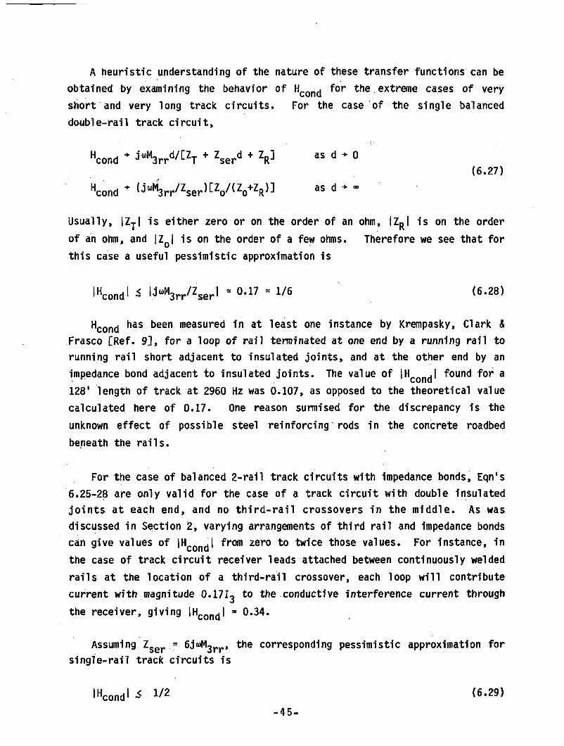
A heuristic understanding of the nature of these transfer functions can be obtained by examining the behavior of Hcon(j for the extreme cases of very short and very long track circuits. For the case of the single balanceddouble-rail track circuit,

Hcond * + Zserd + V as d 0

Hcond J“ 3rr Zser^Zo^Zo+ZR^ as d + “

Usually, |Zj| is either zero or on the order of an ohm, |ZR| is on the order of an ohm, and |ZQ| is on the order of a few ohms. Therefore we see that for this case a useful pessimistic approximation is

lHcondl * li"M3rr/zserl * °-17 ' 176 <«-28>

Hcond has been measured in at least one instance by Krempasky, Clark & Frasco [Ref. 9], for a loop of rail terminated at one end by a running rail to running rail short adjacent to insulated joints, and at the other end by an impedance bond adjacent to insulated joints. The value of IHcon<|I f°und f°r a 128' length of track at 2960 Hz was 0.107, as opposed to the theoretical value calculated here of 0.17. One reason surmised for the discrepancy is the unknown effect of possible steel reinforcing rods in the concrete roadbed beneath the rails.

For the case of balanced 2-rail track circuits with impedance bonds, Eqn's 6.25-28 are only valid for the case of a track circuit with double insulated joints at each end, and no third-rail crossovers in the middle. As was discussed in Section 2, varying arrangements of third rail and impedance bonds can give values of 1HcondI rom zer0 t0 tw1ce those values. For instance, in the case of track circuit receiver leads attached between continuously welded rails at the location of a third-rail crossover, each loop will contribute current with magnitude 0.17I3 to the conductive interference current through the receiver, giving |Hcondl =0.34.

Assuming Zger .= 6j<«>M3rr, the corresponding pessimistic approximation for single-rail track circuits is

IHcondl -< 1/2 (6-23)-45-

Unlike in the case of balanced 2-rail track circuits, here Eqn's 6.25-28 generally will be valid directly for any signal block in which there are no third rail crossovers.

6 .8 Sample Calculations

Table 6.1 shows the results of sample calculations of HCQnd as a function of track circuit length for the following cases:

• Balanced 2-rail audio-frequency track circuit with ZR = Zy = 1 + jO n at f = 3 kHz, with 20 n-kft ballast and NYCTA third-rail spacing.

§ Single-rail track circuit with signal rail adjacent to third rail with ZR = ZT = 1 + jO n at f = 60 Hz, with 20 n-kft ballast and NYCTA third-rail spacing.

These results were obtained by using the FORTRAN 77 program shown in AppendixA. The purpose of showing these results is to provide an order-of-magnitude glimpse at results, and to provide prospective users with a practice example.

6.9 Impedance of the Third rail-DC Return Circuit - Balanced 2-Rail Case

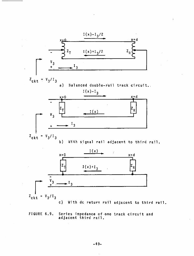
To calculate how much ac current will flow in the third rail, It is necessary to know the total impedance of all track circuits hooked end-to-end from a train to the substation, as pictured in Figure 6.8. Figure 6,9 shows driving-point impedances comprised of track circuits plus third rail. Three cases are shown: balanced two-rail track circuit, single-rail track circuitwith signal rail adjacent to third rail, and single-rail track circuit with dc return rail adjacent to third rail. An extension of the methods used In Sections 6.1-6.7 can be used to calculate the insertion Impedance of a single track circuit in a manner that takes into account finite ballast resistance and the resulting distributed nature of the circuit. As will be shown below, however, if the simplifying assumption is made that Zy = ZR = 0, ballast conduction ceases to be a factor, and the insertion impedance Z . of a single track circuit is then approximately equal to 0.9 uh per meter of length.

-4 6 -

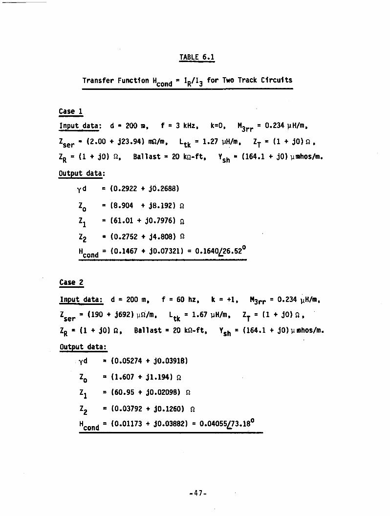
TABLE 6.1

Transfer Function Hcon(J = IR/I3 for Two Track Circuits

Case 1Input data: d = 200 m, f = 3 kHz, k=0, M3rr = 0.234 yH/m,Z$er = (2.00 + J23.94) nfl/m, Ltk = 1.27 yH/m, ZT « (1 ♦ JO)fl ,ZR = (1 + jO) a, Ballast * 20 kn-ft, Y$h = (164.1 + jO) ymhos/m. Output data:

yd = (0.2922 + jO.2688)ZQ = (8.904 + j8.192) a Zx = (61.01 + j0.7976) n Z2 - (0.2752 + j4.808) a HCOnd s (0.1467 + J0.07321) = 0.1640 26.52°

Case 2Input data: d * 200 m, f = 60 hz, k * +1, M3rr = 0.234 yH/m,Zser " ( 19 0 + j692) un/ra» Ltk 58 1 , 6 7 yH/m» ZT ■ ( 1 ♦ jO) n ,ZR * (1 + JO) fl, Ballast * 20 kSl-ft, Ysh * (164.1 + JO)ymhos/m.Output data:

yd = (0.05274 + J0.03918)ZQ = (1.607 + J1•194) aZj = (60.95 + jO.02098) aZ2 = (0.03792 + JO.1260) aHCOnd = (0.01173 + jO.03882) = 0.04055 73.18°

-47-

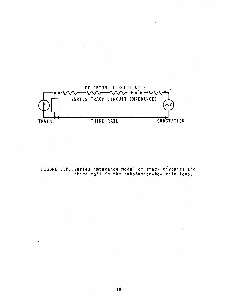
DC RETURN CIRCUIT WITH

FIGURE 6 .8 . .Series impedance model of track circuits and third rail in the substation-to-train loop.

-48-

I(x)-I3/2

'ckt V r3 a) Balanced double-rail track circuit, I(x)-I3

zckt ' V :3 b) With signal rail adjacent to third rail

Zckt V 1 3c) With dc return rail adjacent to third rail.

FIGURE 6.9. Series impedance of one track circuit and adjacent third rail.

-49-

To find Z function of I.

ckt = V3/I3 as shown in Figure 6.9a, we solve for I(x) as ai3, and then find Vg by summing IZ drops in the third rail, the

nearest running rail, lower halves of Zj and ZR, and the induced voltage caused by magnetic flux passing between second and third rails due to currents in the rails:

V3 = CKO) + I3/2](Zt/2) + [1(d) + I3/2](Zr/2)

+ I3dCZ3l'nt + (J“V 2,,n",d23/r3):ld (6.30)

+ [Zlnt + (j«Juo/2ii)ln(d23/r3)] j [I3/2 + I(x)]dxd 0

+ [(j“w0/2ir)ln(d13/d12)]'|[ I3/2 - I(x)]dx

In the above expression, Z3l-nt is the internal impedance per meter of the third rail and r3 is the effective radius of the third rail. Recall from Section 4 that Z1-nt was the internal impedance per meter of the running rail and r and r2 were the effective radii of the running rails. If the techniques described in Section 4 have been used to measure rail impedance, then r. 0 ~ are taken to be equal to the radius of the reference pipe, and the internal impedances are equal to the measured impedances.

Integration of both sides of Eqn. 6.5 yields the relation d£l(x)dx = (l/Zser)[V(0) - V(d) + J“M3rrdI3]

Then, since

V(0) = -I(0)ZT = -iTzT

V(d) = I(d)ZR = IRZR == -I3HcondZT

!3HcondZR

and

where Hcond and H ond are taken from Eqns 6.25,26 with k = 0, the insertion impedance Zckt of the track circuit reduces to:

(6.31)

(6.32)

-50-

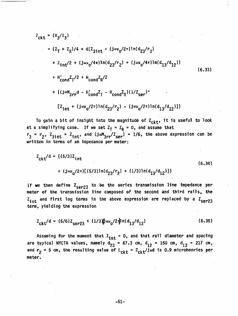
zckt - <yi3>- <ZT + Zr)/4 + d(Z3jnt ♦ <J«y2.)ln<d23/r3)

+ Z)nt/2 + (jo>u0/4iT)ln(d23/r2) + (j»u0/4n)ln(d13/d12))

+ Hi o n d V 2 HcondV2(6.33)

+ (j“M3rrd - HcondZT “ " c o n d V ^ ' W

CZint + (j“,1o^2ir ln (123^r2 " U “*,</2¥*ln d13^d1 2 ^

To gain a bit of insight into the magnitude of Zcjct, it is useful to look at a simplifying case. If we set l j = ZR = 0, and assume thatr3 = r2* Z3int = Zint’ and ^ “M3r/Zser = ^ 6* the above exPression can be written in terms of an impedance per meter:

Zckt/d = « 5/3)Zint (6.34)+ (j<*>u0/2ir)[(5/3)ln(d23/r2) + (1/3) 1 n( d13/d12) ]}

If we then define Zser23 to be the series transmission line impedance per meter of the transmission line composed of the second and third rails, the Zint and flrst lo9 terms in tbe above expression are replaced by a Zger23 term, yielding the expression

W d ' (5/6)Zser23 + < l / 3 H K /2,H <,13/d12) (6.35)

Assuming for the moment that Z1-nt = 0, and that rail diameter and spacing are typical NYCTA values, namely d23 = 67.3 cm, d 2 = 150 cm, d13 = 217 cm, and r2 = 5 cm, the resulting value of Lckt = Zckt/j<od is 0.9 microhenries per meter.

-51-

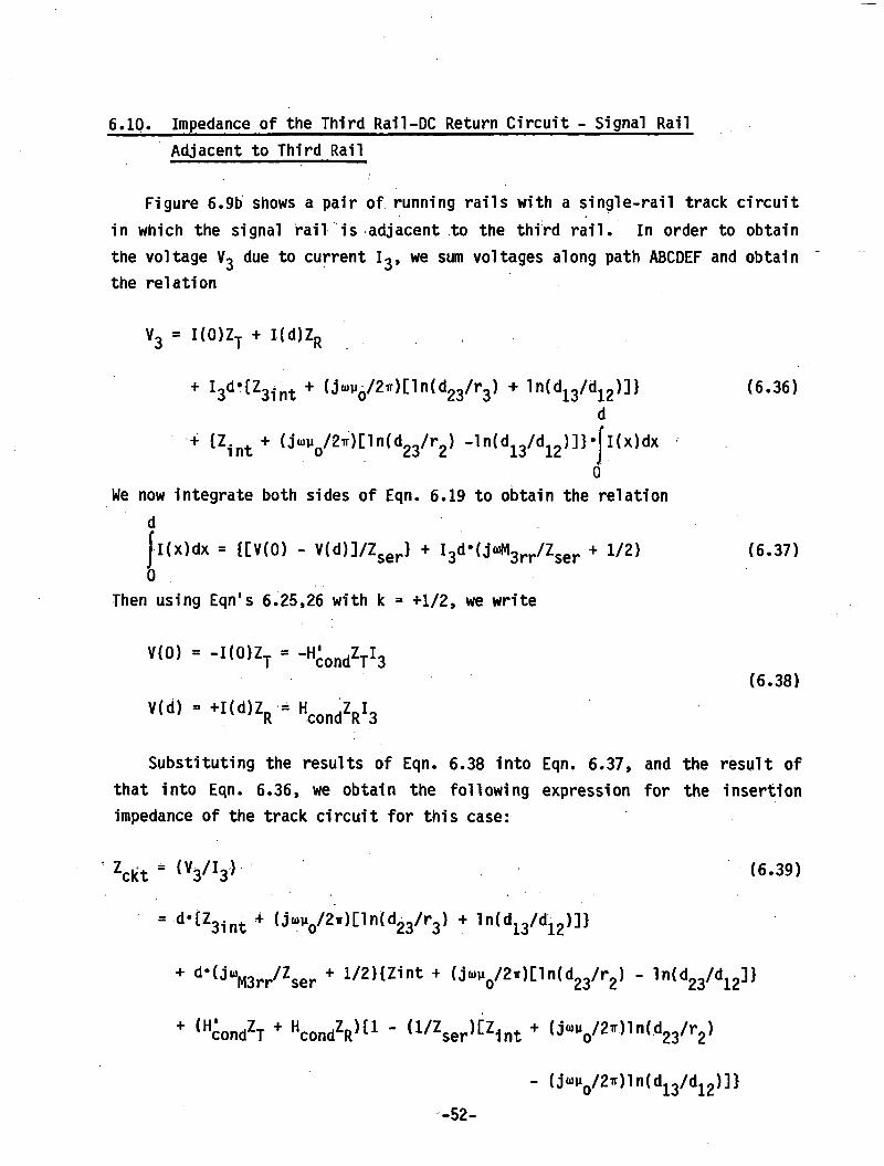
6.10. Impedance of the Third Rail-DC Return Circuit - Signal Rail Adjacent to Third Rail

Figure 6.9b shows a pair of running rails with a single-rail track circuit in which the signal rail is adjacent to the third rail. In order to obtain the voltage V3 due to current I3, we sum voltages along path ABCDEF and obtain the relation

V3 = I(0)ZT + I(d)ZR

+ I3d’^Z3 int + (J n{ d23/r3) + 1 n(d13/d

+ *zi„t + (j»u0/2.)Cln(d23/r2) -ln(d13/d12)]}-

12)3)dI(x)dx

0We now integrate both sides of Eqn. 6.19 to obtain the relation

djl(x)dx = {[V(0) - V(d)]/Zser) + I3d-(jtoM3rr/Zser + 1/2)0

Then using Eqn's 6.25,26 with k = +1/2, we write

(6.36)

(6.37)

V(0) = -i(o)zT ■ -"iondVs

V(d) = +I(d)ZR U 7 Tcond'R3(6.38)

Substituting the results of Eqn. 6.38 into Eqn. 6.37, and the result of that into Eqn. 6.36, we obtain the following expression for the insertion impedance of the track circuit for this case:

left - W - (6.39)

=■ d-{Z3jnt + (j«n.0/2«)[1n(d23/r3) + ln(di3/di2)])

+ d*(j“M3rr/Zser + l/2|lZ1nt + U “M0/2ir)[ln(d23/r2) - ln(d23/d12]}

+ HcondZT + HcondZR){1 “ (1/Zser)[Zint +- (j“u0/2w)ln(d13/d12)]}

-52-

It so happens that for the case where Zj = ZR = 0, Eqn's 6.33 and 6.39 can be put in identical form, and the track circuit's impedance characteristics can once again be described by an approximate inductance per unit length: Lckt = Zckt/jo)d = 0.9 microhenries per meter.

6.11. Impedance of the Third Rail-DC Return Circuit - DC Return Rail Adjacent to Third Rail

Figure 6.9c shows a pair of running rails with a single-rail track circuit in which the dc return rail is adjacent to the third rail. In order to obtain the voltage V3 due to current I3 in this case, we sum voltages along path ABC and obtain the relation

V3 = I3d*{ Z3int + W + (j“V 2,r)Cln(d23/r3) + ln(d23/r2)]}d (6.40)+ {Z.nt + (ja)M0/2ir)[ln(d23/r2) - 1 n(d13/d12)]}*Jl(x)dx

0We now integrate both sides of Eqn. 6.21 and for this case obtain the

relationcI(x)dx = {[V(0) - V(d)]/Zser + I3d-(jo)M3rr - Zser/2)/Zser (6.41)

J0

Then using Eqn's 6.25,26 with k = -1/2, we write

V(0) . -I(0)ZT = -H'ondZTI3

V(d) = +I(d)ZR = HcondZRI3(6.42)

Substituting the results of Eqn. 6.42 into Eqn. 6.41, and the result of that into Eqn. 6.40, we obtain the following expression for the insertion impedance of the track circuit for this case:

-53-

= d'{Z31nt + Z1nt + <j"V2,1[ln(d23/r3) + ,ll(d23/r2l])(6.43)

'3rr/Zser “ 1/2)}

{Z.nt+ (j®u0/2ir)[ln(d23/r2) - lntd^/d^)]}

Once again, if we allow ZR = Zj = 0, Eqn. 6.43 gives exactly the same result as do Eqn's 6.33 and 6.39 when ZR = Zj = 0, and the same value of of 0.9 microhenries per meter.

6.12 Rail Data to Use in Computation

The equations above in Section 6 call for rail radii and internal impedances. There are two possible ways to choose the radii and impedances to use.

The first way to proceed is to use the measurements of rail impedance outlined in Section 3 as a direct source of rail impedance data. In this case, the rail radii r , r2, and r , are all set equal to rcu, the radius of the reference pipe used in the measurements. Then, internal rail impedanceZint ls set e(ua t0

can be set directly equal to Rtk + j“Ltk from Section 3.

A second way to proceed is to use the graphical procedure outlined in Section 5 to find effective values for rail radii and (y/o) ratios. These values are used for r , r2, and r3. Then Eqn. 5.6 is used to calculate approximate effective values of internal rail resistance and inductance. This second way of proceeding is also based on the original rail measurement data,

(6.44)

The corresponding expression is used to find Z_. . for the third rail. Zser

-54-

but the data is fitted to a theoretical model of rail impedance behavior that is then used. This second method can be thought of as a shorthand method, since the original rail data are condensed to a value of radius and (u/o).

6.13 Summary & Conclusions

This section has, introduced the analytical methods for calculating the conductive-interference coupling between third rail and track receivers, in a circuit model that includes distributed ballast conduction effects. Rather idealized situations have been dealt with. Such factors as arbitrary third- rail geometry have been neglected. The existence of third-rail crossovers at arbitrary locations can be dealt with by joining equivalent n-circuits as shown in Figure 6.6, without including Z^ or ZR.

One major result of the analysis presented in this section is the prediction of the impedance of the circuit formed by running rails and dc return rail. This impedance is a series element in the circuit extending from substation to train in which audio-frequency substation harmonic currents and chopper harmonic currents flow. The simplified model that assumes that ZT and ZR are both 0 for every track circuit is also a good worst-case model. This model predicts that the series inductance of this circuit is approximately 0.9 microhenries per meter of circuit length— a value smaller than but comparable to the running-rail transmission-line inductance which has a nominal value of approximately 1.4 microhenries per meter.

The 0.9 yH/meter figure is a conservative one, and can therefore be used in preliminary analysis to find conservative estimates of expected Cl.

-55-

7. INTERFERENCE SOURCE CHARACTERISTICS OF MULTI-CAR TRAINS: CIRCUIT EFFECTS

7.1 The Multi-Car Source

The following sections describe the characteristics of multi-car rapid transit trains as sources of conductive interference. Experience gained to date has been with cars powered by chopper-controlled dc propulsion systems. However, the analytical techniques described are directly applicable to solid-state controlled ac propulsion systems. This section discusses the circuit aspects of multi-car trains. The following section discusses statistical characteristics.

A multi-car train consists of a number of practically identical sources of conductive interference generating signals that add together. Each car in a train will have very nearly the same chopper frequency as the other cars, differing only by tolerances of the frequency standards. The chopper harmonic components of each car will have approximately the same amplitude vs. time characteristics as the other cars in the train.

A multi-car train is a distributed source having the form of a ladder network. Each car provides a rung consisting of the car's Norton equivalent chopper harmonic output current source in parallel with a source inductance. Inter-car inductance provides the series element in the circuit between each rung. Since the interference current from any one car is attenuated as it travels down the ladder, cars will contribute slightly different magnitudes of current to the third rail segment running from the end of the train to the substation. Truman [Ref. 10] has used this model to calculate the circuit characteristics of multi-car trains.

7.2 The Equivalent Circuit of a Multi-Car Train

Figure 7.1 shows a model for the distributed circuit of a multi-car train and a third-rail running-rail loop ending at a substation. Each car is represented by its Norton-equivalent current source and source inductance.

-56-

FIGURE 7.1. The equivalent circuit for conductive interference generation in a multi-car train.

-57-

The source inductance is assumed to be equal to the car's line filter inductance. The series inductance between each train and its neighbors is assumed to be equal to the series inductance per meter of the third-rail running-rail loop times the car length.

This model uses simplifying assumptions that are not believed to harm the qualitative or quantitative nature of the results. In reality, each car is attached to the third rail by two shoes, and to the running rails by 8 wheels. Furthermore, the series inductance between cars in the cirtuit will depend on the placement of propulsion conductors within the car.

In Figure 7.1, the car produces current I ., and has car outputC J

inductance L . The series inductance between one car and the next is L .car ccThe total Norton equivalent source current of an n-car train is In, and theNorton equivalent source inductance of the n-car train is Ln. The values ofL for n = 1, 2, . . . can be found by the recursion relation n .

Ln = {Ln_i + Lcc) I ll-car* L1 Lcar (7.1)

A similar recursion relation can be used to find the expression for source current:

cn + In-lLn-l/(Ln-l + LccJ* h - 'ci

lnlIcl'+ an2lc2 + * * * + ^ Wcn* ann - 1By way of example, these relations were used to calculate Ln and In for

values of n between 1 and 8, assuming Lcar = 500 vh and l_cc = 20 uh:

-58-

4=500 yh, I1=Icl

L2=255 yh, I2=.962Icl+Ic2

L3=177-4 I3=*892Icl+*928Ic2+Ic34=141.5 yh, I4=.801Icl+.882Ic2+.898Ic3+Ic4

(7.3)L5=122.1 yh, I5=.701Ic1+.773Ic2+.787IC3+.876Ic4+Ic5

Lg=110.6 yh, I6=.602Ic1+.664Ic2+.676Ic3+.753Ic4+.859Ic5+Ic6

L?=103.6 yh, I7=.510Ic1+.562Ic2+.572Ic3+.638Ic4+.727Ic5+.847Ic6+Ic7

Lq= 99.1 yh, I8=.427Ic1+.471Ic2+.497Ic3+.535Ic4+.609Ic5+.710Ic6+.838Ic7+Ic8

In the above set of relations, Ln appears to be approaching an asmyptotic value for large n. This value, defined as L^, can be found by solving the relation

L® “ +LCc * Lcar (7.4)

For L = 20 yh and Lr_» = 500 yh, the resulting value is L = 90.5 yh.Wv car ®Me will assume that all the Icn's are phasors of equal amplitude Ic, and

random phase with respect to each other. The maximum magnitude of In, defined as I will occur when all of the individual contributions add in phase:

Jnmax " 1cacl + • • • + acn) (7.5)

For the coefficients given in Eqn. 7.3,

^max *c X2MX = 1-962Ic ‘smax = 2‘82Ic W = 3*58Ic (7.6)W " 4‘14Ic W = 4‘55Ic W = 4*86Ic W = 5‘07Ic

-59-

As n grows large, the value of Inmax also approaches an asmyptotic value I^ax* found by solving the relation

*<*max *c + *«max*-«/^® + (7.7)to obtain the result

^ a x “ Ic^L» + Lcc^Lcc (7.8)

For the values L,* = 90.5 uh and Lcc = 20 uh, the resulting value is I„„av = 5.52K. This asmyptotic behavior results when each car added"fflaX cattenuates as much of the maximum current of the other cars as it then

contributes back.

It is also instructive to calculate the rms value of I , noted as In nrmsSince the individual components of In have randan phase with respect to each other, the mean squared and rms values of In are

I2 = I2(a2. + . . . + a2 ) nrms c' nl nn'T - T . . g2 \ 1/2^rms Iclanl * * * annJ

(7.9)

Based on the coefficients from Eqn. 7.3 in the example above,

*lrms ” ‘c 'znns ‘ l-37Ic ^rms " 1-63Ic '4ms -

W = K86Ic W ’ ‘" c ' bm* * ‘•“ c W ' U m c

(7.10)

In the data above, Inrms is seen to peak and then start declining toward the asmyptote An expression for I is found by squaring each term in an expression equivalent to Eqn. 7.7 to obtain the relation

I2“rms ■c + llrn.sC— /(L* + LCC>12 (7.11)

-60-

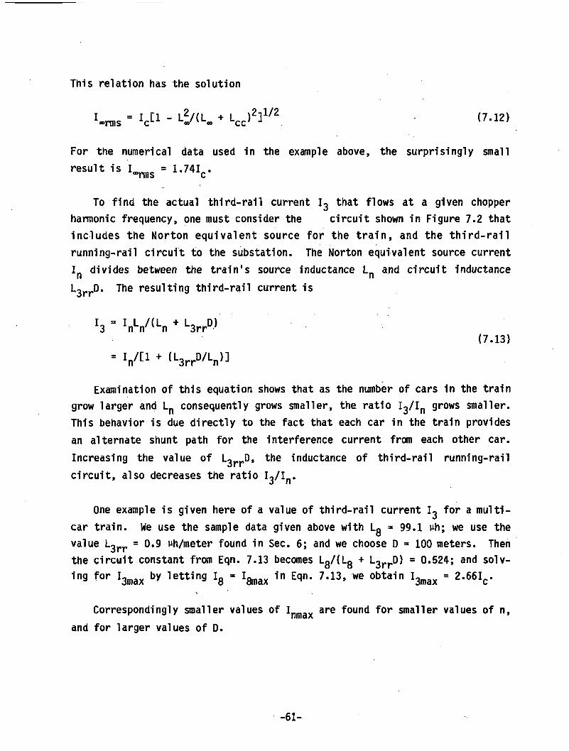
This relation has the solution

I = I [1 - L2/(L + L )2]172 »rms cL <*>'1 «® cc' (7.12)

For the numerical data used in the example above,result is = 1.741 .“rms c

the surprisingly small

To find the actual third-rail current I3 that flows at a given chopper harmonic frequency, one must consider the circuit shown in Figure 7.2 that includes the Norton equivalent source for the train, and the third-rail running-rail circuit to the substation. The Norton equivalent source current In divides between the train's source inductance Ln and circuit inductance L3rrD* The resultin9 third-rail current is

!3 ■ InLn/(Ln + L3rr°>

* V C1 + (L3rrD/Ln>](7.13)

Examination of this equation shows that as the number of cars in the train grow larger and Ln consequently grows smaller, the ratio I3/In grows smaller. This behavior is due directly to the fact that each car in the train provides an alternate shunt path for the interference current from each other car. Increasing the value of L3rrD, the inductance of third-rail running-rail circuit, also decreases the ratio I3/In.

One example is given here of a value of third-rail current I3 for a multi- car train. We use the sample data given above with Lg = 99.1 uh; we use the value L3rr =0.9 uh/meter found in Sec. 6; and we choose D = 100 meters. Then the circuit constant from Eqn. 7.13 becomes Lg/(Lg + L3rrD) = 0.524; and solv-in9 for J3max by lettin9 l8 = W in E9n* 7*13» we obtai" ^max = 2*66Ic*

Correspondingly smaller values of Inmax are found for smaller values of n, and for larger values of D.

-61-

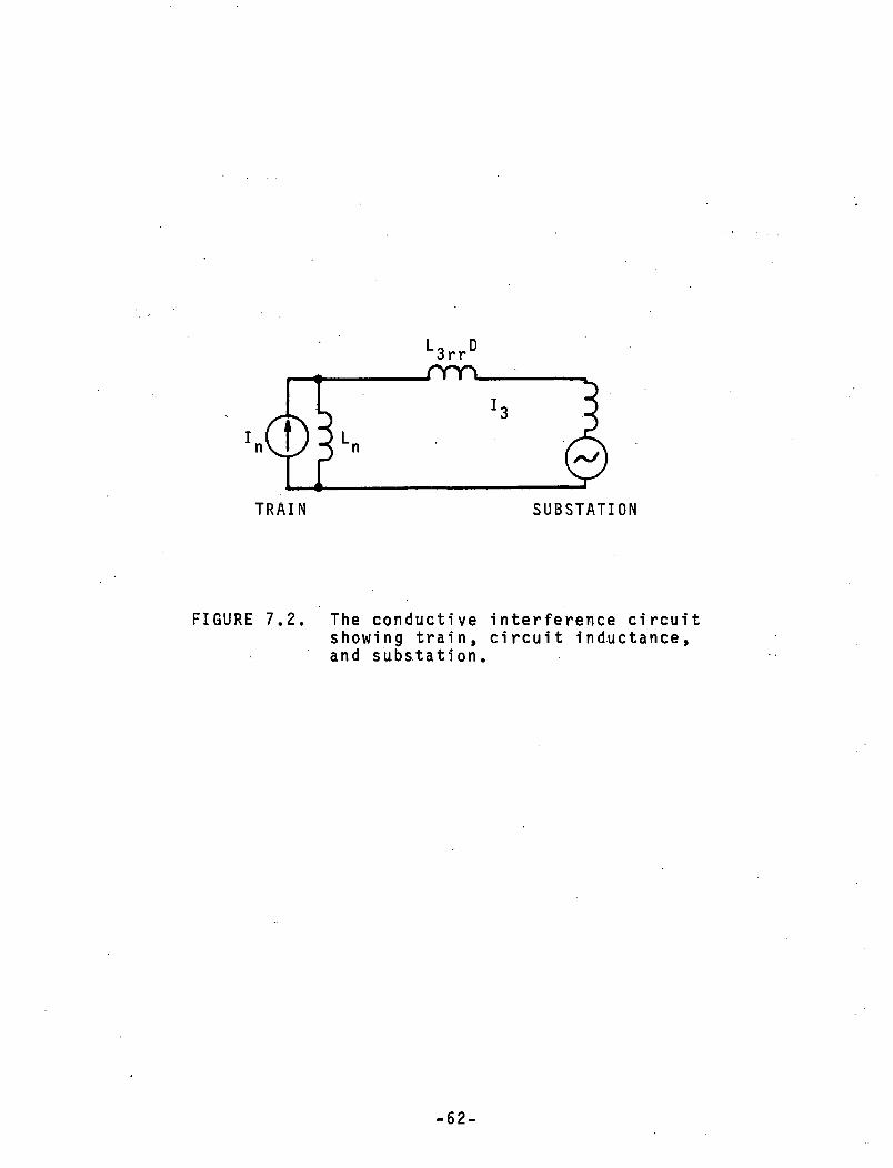
L3rr D

FIGURE 7.2. The conductive interference circuit showing train, circuit inductance, and substation.

-62-

7.3 Summary and Conclusions

In conclusion, we note that a multi-car train has a significantly smaller source inductance than a one-car train. Therefore, the addition of a very moderate amount of circuit inductance— even as little as that of 100 meters of track— can significantly reduce maximum values of chopper harmonic current. This fact should be investigated as a possible means of limiting conductive interference current at those locations where intolerably large values are encountered when trains operate near substation feeds.

Power circuit designers generally try to minimize the inductance of circuits carrying large magnitudes of dc current, because high circuit inductance increases the difficulty of interrupting fault currents in dc circuits. However, the amount of added circuit inductance recommended here is very small compared to the overall inductance in long third-rail circuits.

The analysis in this section only deals with levels of conductive interference contributed by choppers on the rapid transit cars. Substation conductive interference is more directly dealt with. Given the levels of circuit inductance in question, rectifier substations are nearly ideal voltage sources. As n increases and Ln decreases, the total inductance of the circuit in series with the substation decreases, and the level of I3 at substation harmonics increases accordingly.

-63-

8. INTERFERENCE SOURCE CHARACTERISTICS OF MULTI-CAR TRAINS; STATISTICS

8.1 Statistical properties

Each car's chopper control circuitry is independent of other cars. Therefore, at each chopper harmonic frequency in question, the conductive interference signals from the different cars of a train will be randomly phased with respect to each other. In a long-term statistical sense, at any chopper harmonic frequency, the total average noise power will equal the sum of noise powers from the individual cars. In other words, the total rms current will equal the square root of the sum of the squares of the individual components. However, at some time the individual components can be expected to add practically in phase to produce a signal whose amplitude is the direct sum of the individual components. There will be a statistical distribution of interference levels characterized by a probability density function taking on non-zero values from zero to the maximum interference level.

As a function of time, a train's Norton-equivalent conductive interference source current at a particular chopper harmonic frequency f = u>o/2ir can be written as

1n(t) = Ic[llnlcos(“ot + V + a„„cos(a>ftt + e„)] nn o n= I„r„cos(w t + e) c n o

(8.1)

As noted here, the total conductive interference source current for an n-car train is equal to the sum of n independent phasor quantities. The frequency of any particular chopper harmonic typically will vary by a fraction of a hertz from car to car. This will cause the values of e , eg, ..., in the equation above to vary slowly with time. Therefore, over the short time span it takes for a train to accelerate from rest up to the speed at which the choppers stop chopping, phase relations between the interference current phasors of cars at a particular chopper harmonic will remain approximately fixed. However, over the longer period between starts, phases will have a chance to re-randomize.

-64-

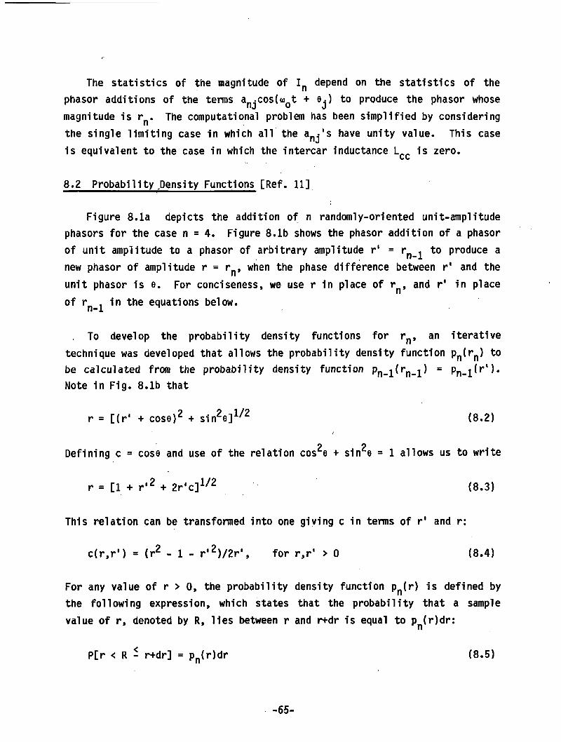
The statistics of the magnitude of In depend on the statistics of the phasor additions of the terms a -cos(u> t + e.) to produce the phasor whose

IIJ w Jmagnitude is rn« The computational problem has been simplified by considering the single limiting case in which all the anj.'s have unity value. This case is equivalent to the case in which the intercar inductance L is zero.

8.2 Probability density Functions [Ref. 11]

Figure 8.1a depicts the addition of n randomly-oriented unit-amplitudephasors for the case n = 4. Figure 8.1b shows the phasor addition of a phasorof unit amplitude to a phasor of arbitrary amplitude r' = rn_ to produce anew phasor of amplitude r = rn, when the phase difference between r' and theunit phasor is e. For conciseness, we use r in place of rn, and r' in placeof r .in the equations below. n-1

To develop the probability density functions for rn, an iterative technique was developed that allows the probability density function pn( ) to be calculated from the probability density function pn_1 {r*n_i) = pn_i(r1). Note in Fig. 8.1b that

r = [(r1 + cose)2 + sin2e]1/2 (8.2)9 9Defining c = cose and use of the relation cos e + sin e = 1 allows us to write

r = [1 + r'2 + 2r'c]1/2 (8.3)

This relation can be transformed into one giving c in terms of r' and r:

c(r,r') = (r2 - 1 - r'2)/2r‘, for r,r' > 0 (8.4)

For any value of r > 0, the probability density function Pn(r) is defined by the following expression, which states that the probability that a sample value of r, denoted by R, lies between r and r+dr is equal to pn(r)dr:

P[r < R - r+dr] = pn(r)dr (8.5)

-65-

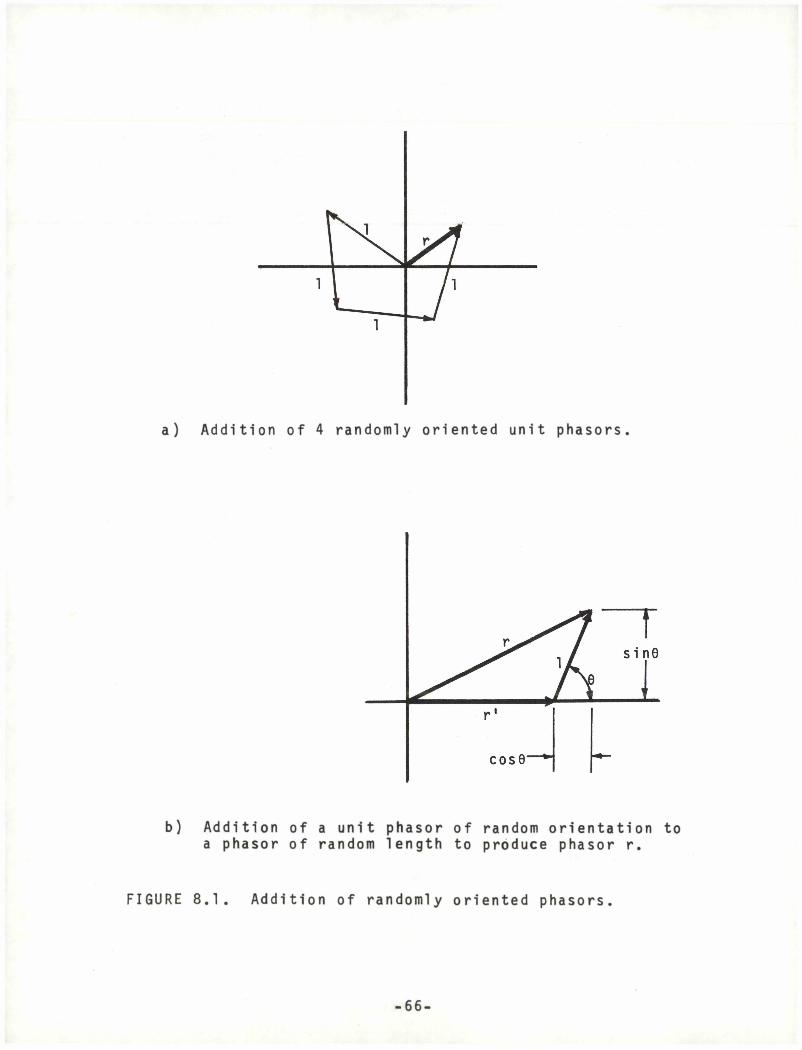
a) Addition of 4 randomly oriented unit phasors.

b) Addition of a unit phasor of random orientation to a phasor of random length to produce phasor r.

FIGURE 8.1. Addition of randomly oriented phasors.

-66-

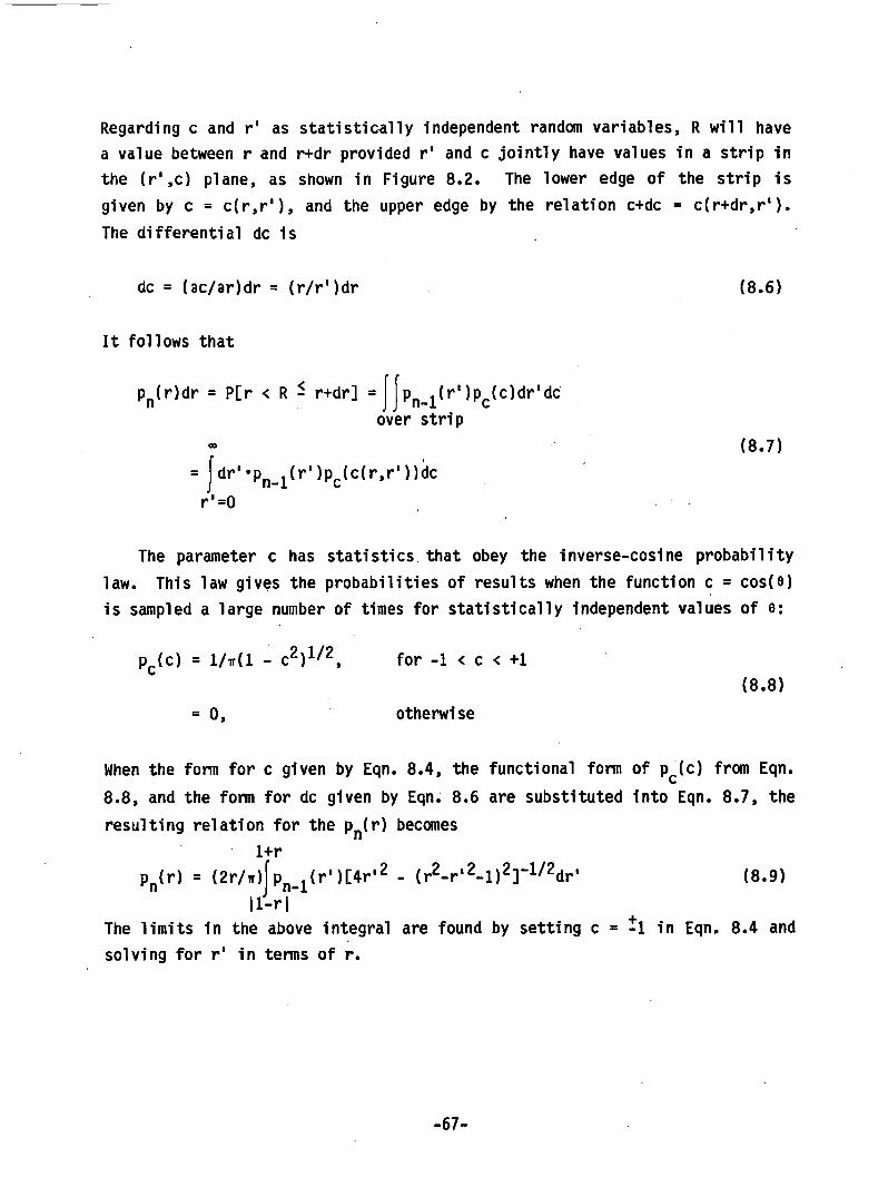
Regarding c and r' as statistically independent randan variables, R will have a value between r and r+dr provided r' and c jointly have values in a strip in the (r',c) plane, as shown in Figure 8.2. The lower edge of the strip is given by c = c(r,r‘), and the upper edge by the relation c+dc = c(r+dr,r'). The differential dc is

dc = (ac/ar)dr = (r/r')dr

It follows that

Pn(r)dr = P[r < R - r+dr] = pn_i (r' )pc(c)dr'dc over strip

dr' *pn (r' )Pc(c(r,r' ))dcr =0

(8.6)

(8.7)

The parameter c has statistics that obey the inverse-cosine probability law. This law gives the probabilities of results when the function c = cos(e) is sampled a large number of times for statistically independent values of 0:

Pc(c) = l/ir(l - c2)1/2, for -1 < c < +1

= 0, otherwi se(8.8)

When the form for c given by Eqn. 8.4, the functional form of p.(c) from Eqn. 8.8, and the form for dc given by Eqn. 8.6 are substituted into Eqn. 8.7, the

>n fc 1+r

resulting relation for the Pn(r) becomes

Pn(r) = (2r/ir) pn l(r')[4r'2 - (r2-r,2-l)2]_1/2dr' (8.9)ll-r I

The limits in the above integral are found by setting c = il in Eqn. 8.4 and solving for r' in terms of r.

-67-

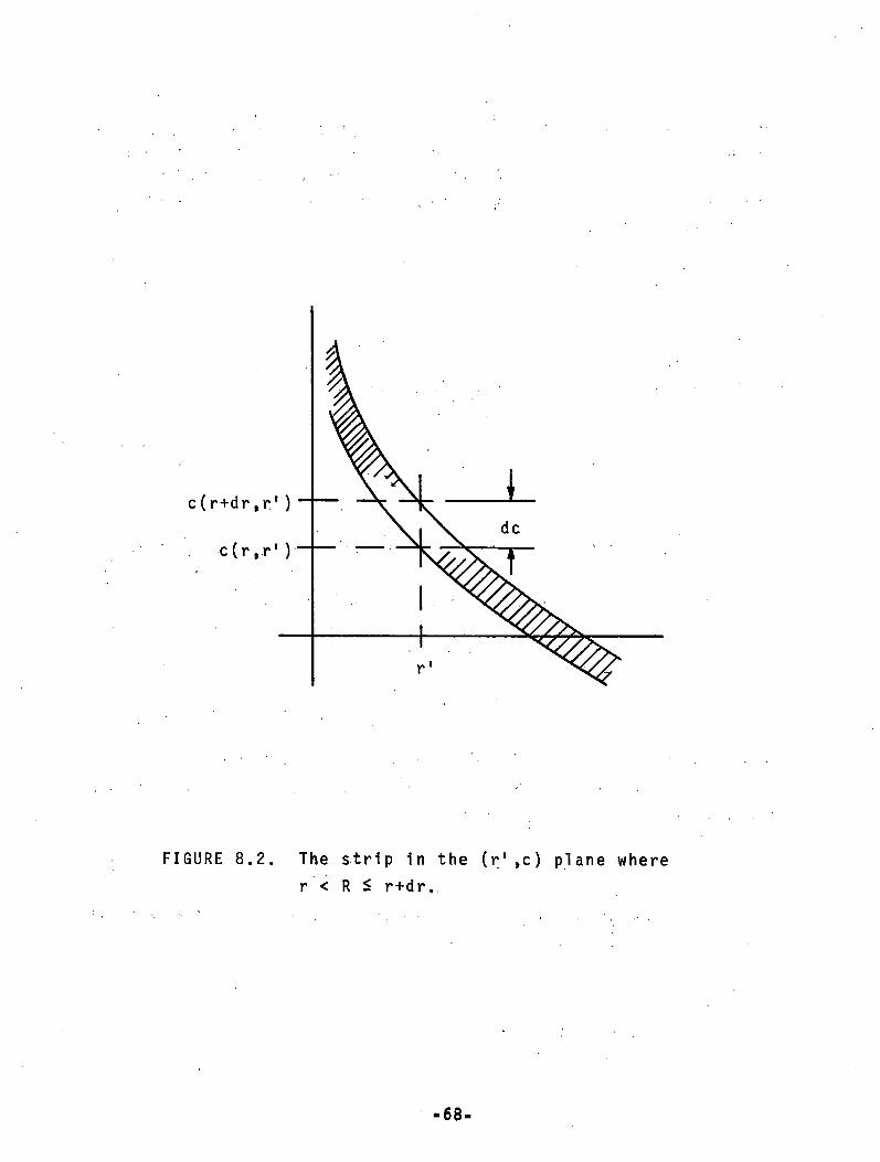
FIGURE 8.2. The strip in the (r',c) plane where r < R £ r+dr.

- 6 8 -

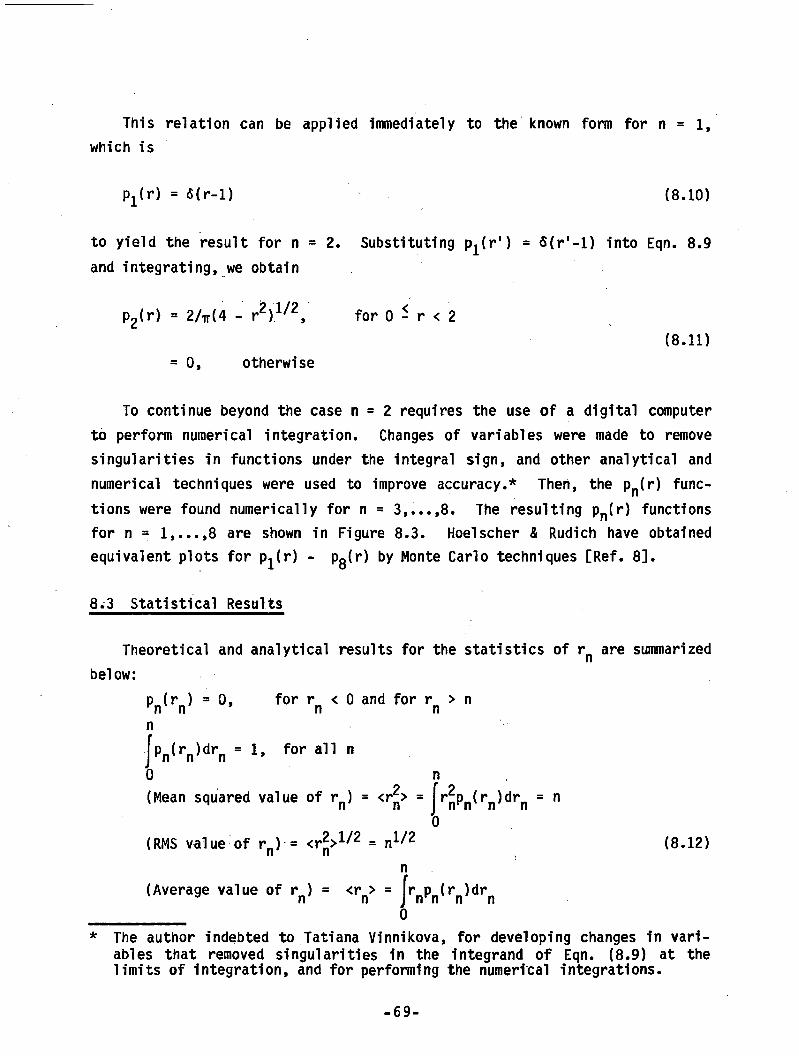
This relation can be applied immediately to the known form for n = 1, which is

Px(r) = S(r-l) (8.10)

to yield the result for n = 2. Substituting p1 (r') = 6(r'-l) into Eqn. 8.9 and integrating, we obtain

P2(r) = 2/ir(4 - r2)1/2, for 0 - r < 2

= 0, otherwise(8.11)

To continue beyond the case n = 2 requires the use of a digital computer to perform numerical integration. Changes of variables were made to remove singularities in functions under the integral sign, and other analytical and numerical techniques were used to improve accuracy.* Then, the Pn(r) functions were found numerically for n = 3,...,8. The resulting pn(r) functions for n = 1,...,8 are shown in Figure 8.3. Hoelscher & Rudich have obtained equivalent plots for p^(r) - Pg(r) by Monte Carlo techniques [Ref. 8].

8.3 Statistical Results

Theoretical and analytical results for the statistics of rp are summarized below:

p (r ) = 0, for r < 0 and for r > n n n n nnJpn(rn)drn = lf for a11 n 0 n(Mean squared value of rn) = <r2> = JrpPn(^n)drn = n

0(RMS value of rn) = <r^>1/r2 = n ^ 2 (8.12)

n(Average value of r ) = <r > = r p (r )drn n J n n n n_ _ _ _ _ _ _ _ 0

* The author indebted to Tatiana Vinnikova, for developing changes in variables that removed singularities in the integrand of Eqn. (8.9) at the limits of integration, and for performing the numerical integrations.

-69-

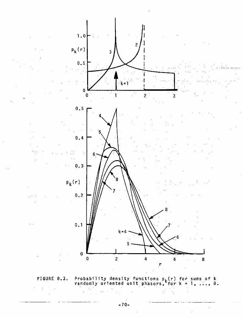
1.0

FIGURE 8.3. Probability density functions p.(r) for sums of k randomly oriented unit phasors, for k = 1 * ...» 8.

- 7 0 -

(8.12, cont'd)<rl> = 1 <r2> = 4/ir = 1.27 <r^> = 1.58

<r4> = 1.80 <rg> = 2.01 <rg> = 2.20

<r7> = 2.37 <rQ> =2.53

8.4 Behavior for Large Values of n

For n » 1, the probability density function p (r) approaches the Rayleigh2 nprobability density function, with parameter o = n/2:

pR(r) = (r/a2)exp(-r2/2a2), for r - 0

= 0, for r < 0(8.13)

In other words, as n grows large, the sum of n randomly phased unit-amplitude phasors has an envelope whose statistics are the same as the envelope function of a narrow-band gaussian random process. This fact is shown graphically in

pFig. 8.4, in which pQ(r) and the Rayleigh pdf pR(r) = (r/4)exp(-rV8) are plotted together.

8.5 Probability of r Exceeding a Particular Value

The function that gives the probability that a sample value R is less thanor equal to r is the probability distribution function Pn(r)

PER - r] = Pn(r) = pn(x)dx (8.14)

Me can take the lower limit of the above integration to be zero.

The function that gives the probability that a sample value R is greater than r is the complementary probability distribution function P^(r):

oo

PER > r] = Pp(r) = pn(x)dx (8.15)Jr

Numerically derived plots of P^(r) are shown in Fig. 8.5 for n = 2,...,8.

-71-

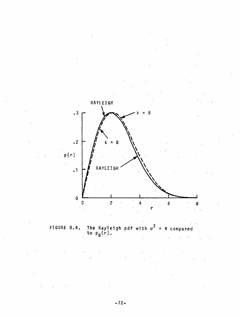
RAYLEIGH.3

.2

p(r)

.1

0

FIGURE 8.4. The Rayleigh pdf with a2 = 4 comparedto P8 (r).

-72-

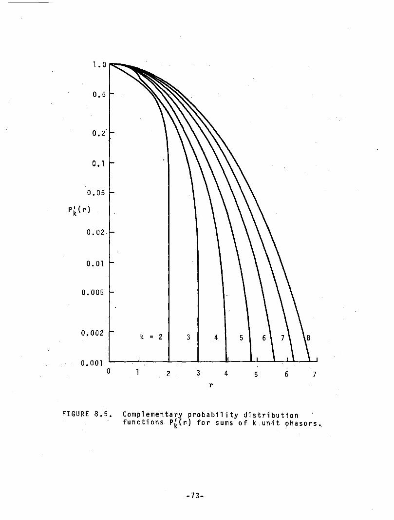
FIGURE 8.5. Complementary probability distributionfunctions PjJ(r) for sums of k.unit phasors.

-73-

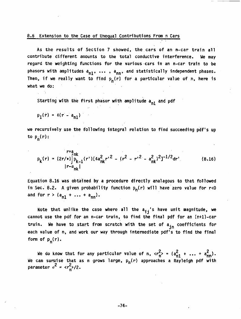
8.6 Extension to the Case of Unequal Contributions From n Cars

As the results of Section 7 showed, the cars of an n-car train all contribute different amounts to the total conductive interference. We may regard the weighting functions for the various cars in an n-car train to be phasors with amplitudes anl, ... , ann, and statistically independent phases. Then, if we really want to find pn(r) for a particular value of n, here is what we do:

Starting with the first phasor with amplitude anl and pdf

p1(r) = 6(r - anl)

we recursively use the following integral relation to find succeeding pdf's up to Pn(r):

pk<r)r+a . rnk(2r/ir) Ir-apk-l(r')[4ankr'2nlJ

(r2 - r'2 - a2 )2]-1^2dr' J nk (8.16)

Equation 8.16 was obtained by a procedure directly analagous to that followed in Sec. 8.2. A given probability function pn(r) will have zero value for r<0 and for r > (anl + ... + ann).

Note that unlike the case where all the a..'s have unit magnitude, we* Jcannot use the pdf for an n-car train, to find the final pdf for an (n+l)-car

train. We have to start from scratch with the set of a. coefficients forjneach value of n, and work our way through intermediate pdf's to find the finalform of p (r). n

9 9 9We do know that for any particular value of n, <r|j> = (a^ + ... + a^n).We can surmise that as n grows large, pn(r) approaches a Rayleigh pdf with2 2 11 parameter o = <rn>/2.

-74-

8.7 Statistics Summary

The statistical results above represent formal answers to a highly idealized problem. Nonetheless, these results can serve as a guide to our thinking about expected conductive chopper interference levels from multi-car trains. Clearly, the writers of specifications for limits on conductive chopper interference must be precise in the statement of what their limits pertain to. For instance, when limits for one car are extrapolated to an n-car train, we must state whether the the limit for the train is a maximum figure or an rms figure. In addition, we must remember that in this problem, "rms" refers to an averaging process over a statistical ensemble, and not to an averaging process over the period of a predictable periodic signal.

We saw in Section 7 that at a particular chopper harmonic, the maximum conductive interference current flowing in the third rail from an n-car train would be a fraction of the current from one car times n. In this section, wesaw that actual values of third-rail current will be randomly distributed/between zero and that maximum value.

Perhaps it is of comfort when measuring conductive chopper interference from multi-car trains in the field, to realize that the randomness in the data is not necessarily due to experimental error, but is at the heart of the process itself.

-75-

9. MEASUREMENT OF CONDUCTIVE INTERFERENCE; .TECHNIQUES 3 DATA

9.1 Recommended Practices

A draft set of recommended practices has been developed under the aegis of the Rail Transit Electromagnetic Interference Technical Working Group (TWG). This committee's membership includes representatives of rapid transit signaling and propulsion manufacturers, transit industry consultants, and university and government researchers. TWG is organized under the auspices of DOT/UMTA. TWG has prepared draft Recommended Practices that describe methods for observing, recording, and analyzing conductive interference in rapid transit signaling systems, and for measuring the susceptibility of signaling systems to conductive interference [Ref. 12]. The techniques described below for observing and recording conductive interference are described in large part in the Recommended Practices. Measurement techniques are summarized below.

9.2 Instrumentation

Conductive interference in rapid transit signaling is in the form of power-frequency or audio-frequency current components superimposed on dc propulsion current. Propulsion current levels can be large— thousands of amperes. Signaling current levels are smal 1— amperes in the case of power-frequency signaling, or tens to hundreds of milliamperes in the case of audio-frequency signaling. Therefore, special means must be used to observe conductive interference currents whose magnitudes will be of the same order as those of signaling currents.

The primary tool used for measuring conductive interference currents is the Hall-effect servo current sensor. The type used in this activity is the LEM Transfoshunt}. Transfoshunt models having maximum dc current capability of 1200 amperes and 10,000 amperes have been used in this program— the lower current model aboard single rapid transit cars, and the higher current model in rectifier substations.

-76-

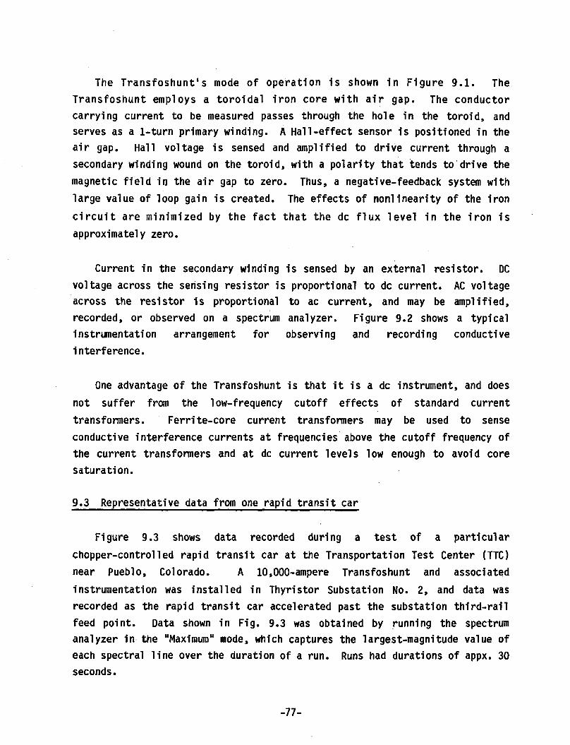
The Transfoshunt's mode of operation is shown in Figure 9.1. The Transfoshunt employs a toroidal iron core with air gap. The conductor carrying current to be measured passes through the hole in the toroid, and serves as a 1-turn primary winding. A Hall-effect sensor is positioned in the air gap. Hall voltage is sensed and amplified to drive current through a secondary winding wound on the toroid, with a polarity that tends to drive the magnetic field in the air gap to zero. Thus, a negative-feedback system with large value of loop gain is created. The effects of nonlinearity of the iron circuit are minimized by the fact that the dc flux level in the iron is approximately zero.

Current in the secondary winding is sensed by an external resistor. DC voltage across the sensing resistor is proportional to dc current. AC voltage across the resistor is proportional to ac current, and may be amplified, recorded, or observed on a spectrum analyzer. Figure 9.2 shows a typical instrumentation arrangement for observing and recording conductive interference.

One advantage of the Transfoshunt is that it is a dc instrument, and does not suffer from the low-frequency cutoff effects of standard current transformers. Ferrite-core current transformers may be used to sense conductive interference currents at frequencies above the cutoff frequency of the current transformers and at dc current levels low enough to avoid core saturation.

9.3 Representative data from one rapid transit car

Figure 9.3 shows data recorded during a test of a particular chopper-controlled rapid transit car at the Transportation Test Center (TTC) near Pueblo, Colorado. A 10,000-ampere Transfoshunt and associated instrumentation was installed in Thyristor Substation No. 2, and data was recorded as the rapid transit car accelerated past the substation third-rail feed point. Data shown in Fig. 9.3 was obtained by running the spectrum analyzer in the "Maximum" mode, which captures the largest-magnitude value of each spectral line over the duration of a run. Runs had durations of appx. 30 seconds.

-77-

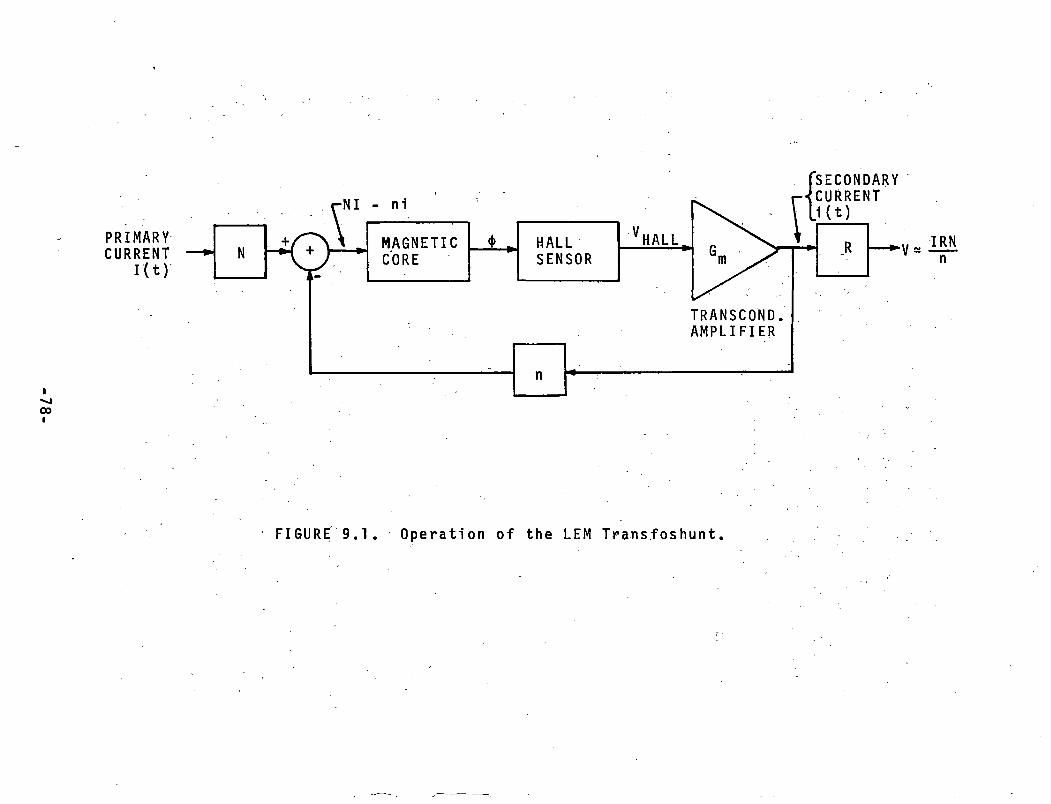
I*-400I

PRIMARYCURRENTK t )IRNn

FIGURE 9.1. Operation of the LEM Transfoshunt.

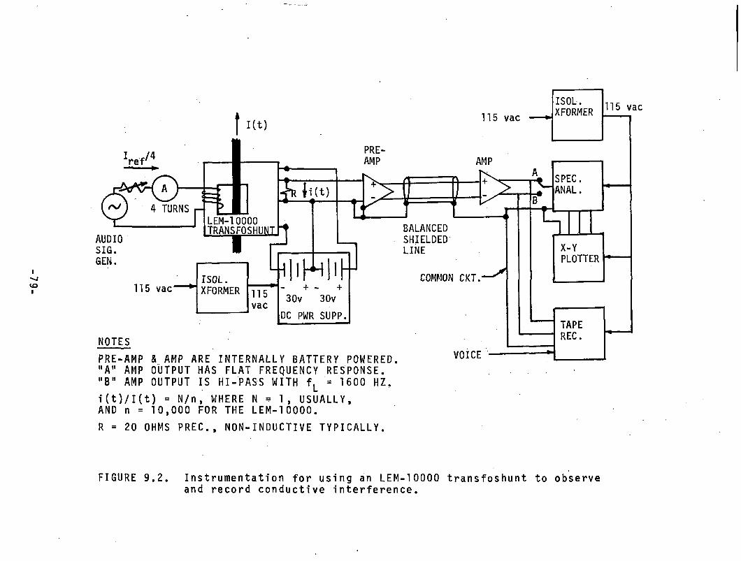
VOI

115 vac

W 4

AUDIOSIG.GEN.

115 vac"

NOTESPRE-AMP "A" AMP "B" AMP

& AMP ARE INTERNALLY BATTERY POWERED. OUTPUT HAS FLAT FREQUENCY RESPONSE.VOICE

OUTPUT IS HI-PASS WITH f, 1600 HZ.1(t)/I(t) = N/n, WHERE N = 1, USUALLY,AND n = 10,000 FOR THE LEM-10000.R = 20 OHMS PREC., NON-INDUCTIVE TYPICALLY.

. Instrumentation for using an LEM-10000 transfoshunt to observe and record conductive interference.FIGURE 9.2

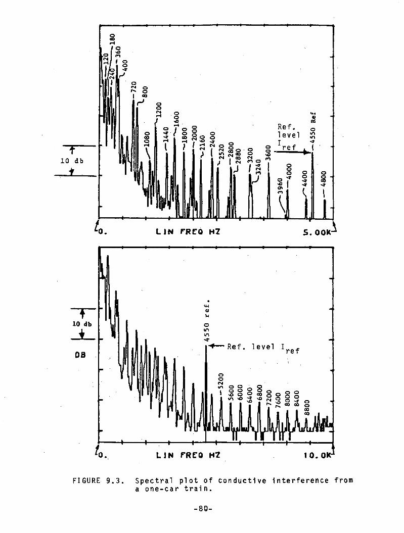
L I N F R C Q H 2 1 0. 0KJ

FIGURE 9.3. Spectral plot of conductive interference from a one-car train.-80-

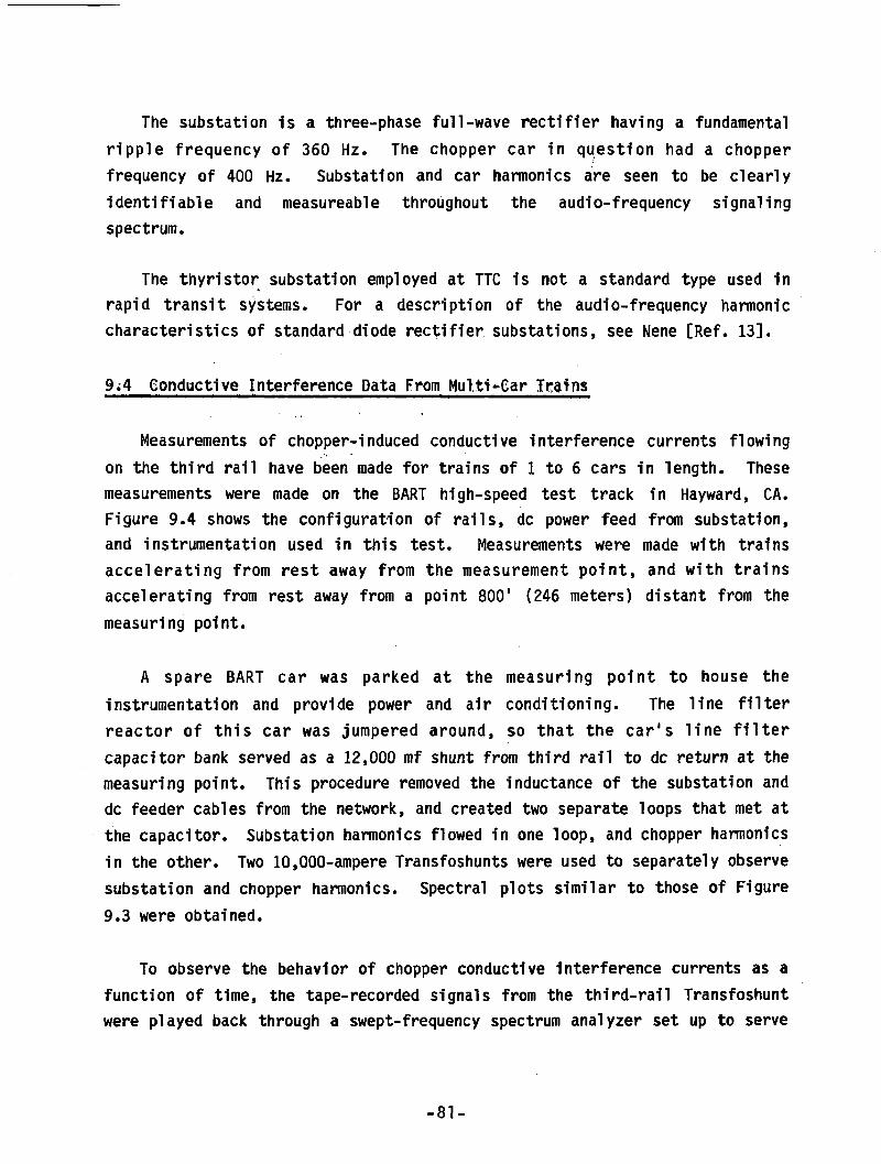
The substation is a three-phase full-wave rectifier having a fundamental ripple frequency of 360 Hz. The chopper car in question had a chopper frequency of 400 Hz. Substation and car harmonics are seen to be clearly identifiable and measureable throughout the audio-frequency signaling spectrum.

The thyristor substation employed at TTC is not a standard type used in rapid transit systems. For a description of the audio-frequency harmonic characteristics of standard diode rectifier substations, see Nene [Ref. 13].

9.4 Conductive Interference Data From Multi-Car Trains

Measurements of chopper-induced conductive interference currents flowing on the third rail have been made for trains of 1 to 6 cars in length. These measurements were made on the BART high-speed test track in Hayward, CA. Figure 9.4 shows the configuration of rails, dc power feed from substation, and instrumentation used in this test. Measurements were made with trains accelerating from rest away from the measurement point, and with trains accelerating from rest away from a point 800' (246 meters) distant from the measuring point.

A spare BART car was parked at the measuring point to house the instrumentation and provide power and air conditioning. The line filter reactor of this car was jumpered around, so that the car's line filter capacitor bank served as a 12,000 mf shunt from third rail to dc return at the measuring point. This procedure removed the inductance of the substation and dc feeder cables from the network, and created two separate loops that met at the capacitor. Substation harmonics flowed in one loop, and chopper harmonics in the other. Two 10,000-ampere Transfoshunts were used to separately observe substation and chopper harmonics. Spectral plots similar to those of Figure9.3 were obtained.

To observe the behavior of chopper conductive interference currents as a function of time, the tape-recorded signals from the third-rail Transfoshunt were played back through a swept-frequency spectrum analyzer set up to serve

- 8 1 -

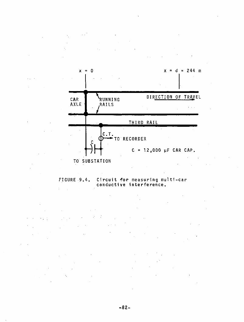
x = 0 X d = 244 m

DIRECTION OF TRAVEL

THIRD RAILJC.T.O - 1►TO' RECORDER

■ ^ h h

TO SUBSTATIONC = 12*000 y F CAR CAP

FIGURE 9.4. Circuit for measuring multi-car conductive interference.

8 2 -

as a narrow-band filter and detector. The spectrum analyzer was adjusted to zero Hz sweep width, 30 Hz resolution bandwidth, arid 5 seconds/division sweep speed. The vertical scale was linear, and was calibrated by using a known reference signal injected by means of a multi-turn reference winding on the Transfoshunt.

Data are shown for the fundamental chopper harmonic of 218 Hz, and the 7th chopper harmonic at 1526 Hz. Note that the vertical scale differs from picture to picture.

Figure 9.5a shows 218 Hz data for one car starting from rest at the measuring point. Note that harmonic current increases and then decreases as the chopper duty cycle starts from a low value and increases to nearly 100%. Maximum harmonic content is reached when duty cycle is 50%. Ten seconds after starting, there is a step increase in current when the field shunting occurs.

Comparing Figures 9.5a-f for 1 to 6 cars respectively, one observes a random behavior of peak amplitude with number of cars, as theory predicts. In studying this data, one should remember that over the 30-second interval 1n each run for which significant harmonic current exists, the relative phases of interference currents from different cars do not have a chance to change with respect to each other. However over the minutes required prepare for the next run, the phases do have time to re-randomize.

In observing the effect at 218 Hz of moving the starting point from 0 to 800' away for a specific number of cars, one observes the general tendency for the increased distance to have a far greater effect in reducing peak current for the longer trains than for the shorter. This is once again in keeping with the analytical results outlined in Section 7.

Figures 9.5g and h, taken at 1526 Hz for 1 and 2 cars, demonstrate clearly an additional dynamic effect— the periodic variation in strength of a given harmonic as a function of duty cycle. The effects of increasing the number of cars, and of moving the starting point, are seen to be generally the same at 1526 Hz as at 218 Hz.

-83-

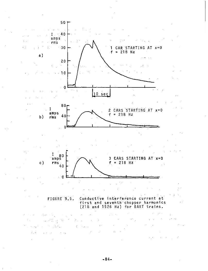
5 0 r

I 40 -

b)Iampsrras

c)

FIGURE 9.5. Conductive interference current at first and seventh chopper harmonics (218 and 1526 Hz) for BART trains.

-84-

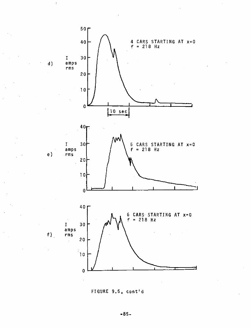
50

FIGURE 9.5, cont'd

85-

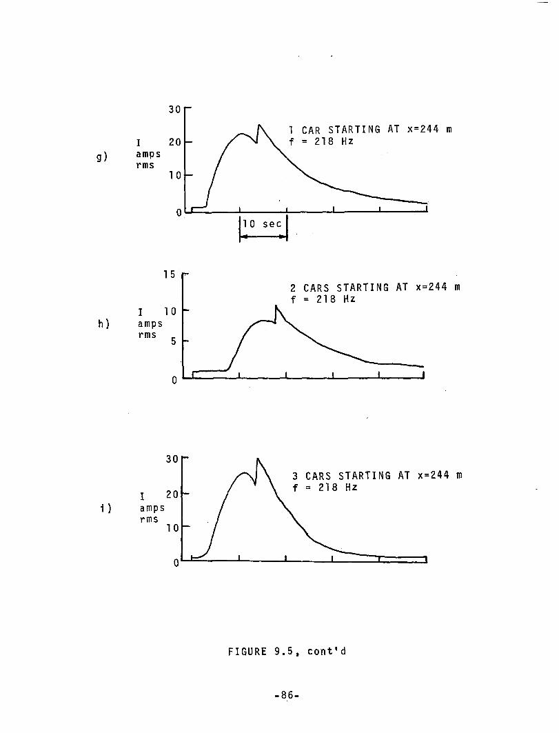
3 0 r

i)Iampsrms

FIGURE 9.5, cont'd

-86-

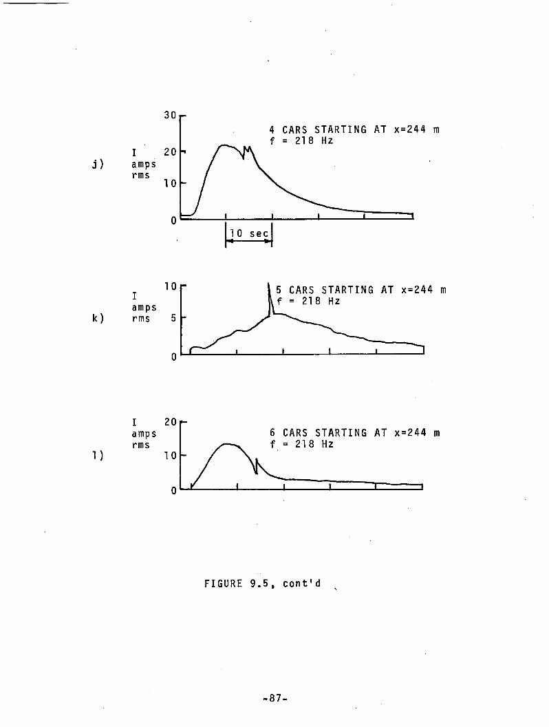
j )Iampsrms

1)

Iampsrms

FIGURE 9.5, cont'd

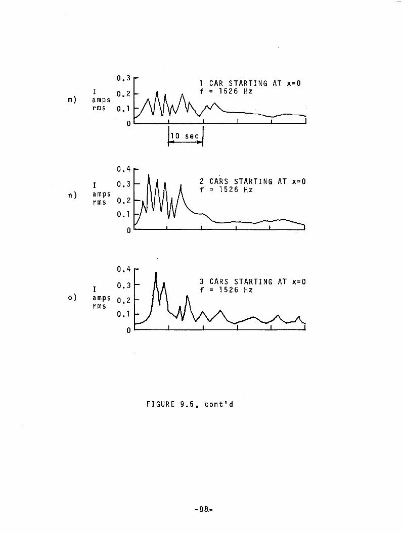
Iampsrms

Iampsrms

FIGURE 9.5, cont'd

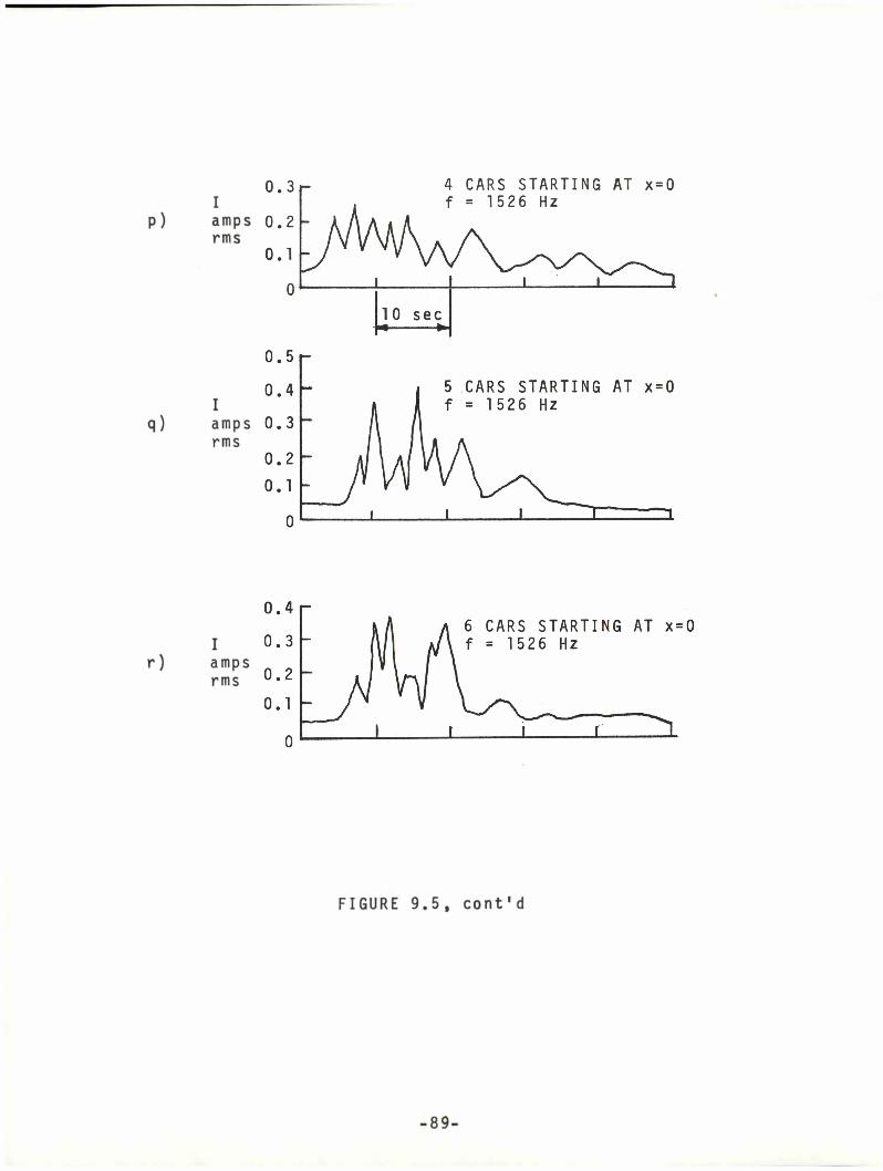
p)

q)

iamp;rms

Iamp:rms

r)Iampsrms

FIGURE 9.5, cont'd

-89-

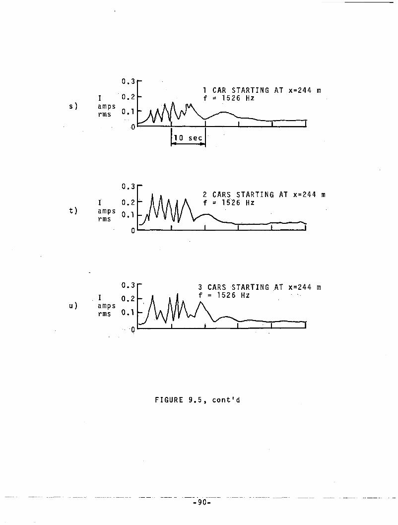
s)

0.31 CAR STARTING AT x=244 m f = 1526 Hz

u)Iampsrms

FIGURE 9.5, cont'd

- 9 0 -

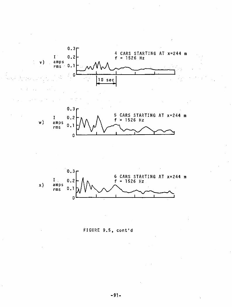
0.30.2 4 CARS STARTING AT x=244 m f = 1526 Hz

FIGURE 9.5, cont'd

91

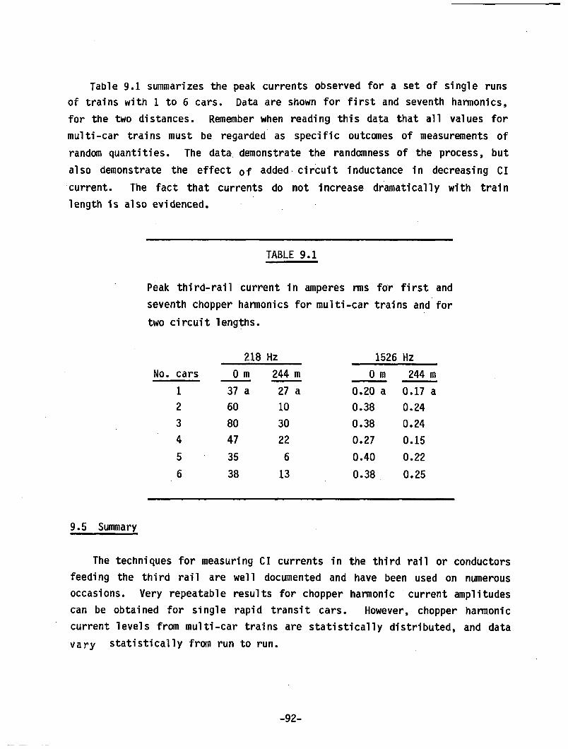
Table 9.1 summarizes the peak currents observed for a set of single runs of trains with 1 to 6 cars. Data are shown for first and seventh harmonics, for the two distances. Remember when reading this data that all values for multi-car trains must be regarded as specific outcomes of measurements of random quantities. The data demonstrate the randomness of the process, but also demonstrate the effect 0f added circuit inductance in decreasing Cl current. The fact that currents do not increase dramatically with train length is also evidenced.

TABLE 9.1

Peak third-rail current in amperes rms for first and seventh chopper harmonics for multi-car trains and for two circuit lengths.

218 Hz 1526 HzNo. cars 0 m 244 m 0 m 244 m

1 37 a 27 a 0.20 a 0.17 a2 60 10 0.38 0.243 80 30 0.38 0.244 47 22 0.27 0.155 35 6 0.40 0.226 38 13 0.38 0.25

9.5 Summary

The techniques for measuring Cl currents in the third rail or conductors feeding the third rail are well documented and have been used on numerous occasions. Very repeatable results for chopper harmonic current amplitudes can be obtained for single rapid transit cars. However, chopper harmonic current levels from multi-car trains are statistically distributed, and data vary statistically from run to run.

-92-

Rigorous correlation of field data with the statistical results of Sec. 8 would require the collection of much more data— enough to provide a statistical data base. This data would have to be collected under the same carefully controlled conditions as detailed in Sec. 9.4.

Due to the cost and complexity of making measurements, it was only possible to make- one good run from each starting location for each train length. However, the results of the data do fit in a general fashion with what is predicted by the circuit analysis and statistics outlined in previous sections of this report.

-93-

10. CONCLUSION

Conductive interference in rapid transit signaling is a problem that is complex, due to the physically large nature of circuits, and the number of separate circuit elements involved. In addition, statistical considerations must be taken into account. However, the individual aspects of conductive interference are tractable as far as analysis and testing is concerned.

We have examined different aspects of this problem and the contributions of many workers from a common perspective. Circuit models have been developed for circuits comprised of track and third rail using standard transmission line and lumped-circuit techniques.

Recommended practices have been developed for observing and measuring Cl currents, and the techniques contained in these have been used to collect data contained in this report.

The efforts reported here were made in response to specific Cl problems that arose in new rapid transit systems. The results that have been obtained should assist in the avoidance or solution of similar Cl problems in the future. For instance, Section 6 showed that in the case of balanced two-rail track circuits, the injection of Cl currents into the receiver leads is dependent on the asymmetrical location of the third rail with respect to the running rails. One way to avoid this potential problem would be the use of overhead catenaries instead of third rails. This is but one example. In the design of rapid transit systems, every single aspect of design should be examined at the outset for its impact on Cl.

-94-

APPENDIX

FORTRANCONDUCTIVE

PROGRAM FOR CALCULATING THE INTERFERENCE TRANSFER FUNCTION

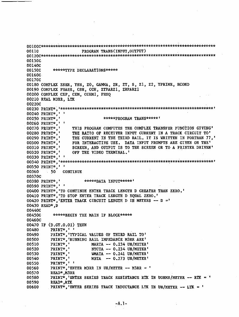
00100C************************************************************************* OOllO PROGRAM TRANS(INPUT,OUTPUT)00120C*************************************************************************00130C00140C00150C *****TYPE declarations*****00160C00170C00180 COMPLEX ZSER, YSH, ZO, GAMMA, ZR, ZT, S, Zl, Z2, YPRIME, HCOND00190 COMPLEX PHASE, CSH, CCH, ZTPARZl, ZRPARZl00200 COMPLEX CXP, CXM, CCHM1, PHSQ00210 REAL M3RR, LTK00220C00230 PRINT*,*****************************************************************' 00240 PRINT*,'00250 PRINT*,'00260 PRINT*,'00270 PRINT*,'00280 PRINT*,'00290 PRINT*,'00300 PRINT*,'00310 PRINT*,'00320 PRINT*,'00330 PRINT*,'00340 PRINT*,'00350 PRINT*,'00360 5000370C00380 PRINT*,'00390 PRINT*,' '00400 PRINT*,'TO CONTINUE ENTER TRACK LENGTH D GREATER THAN ZERO.'00410 PRINT*,'TO STOP ENTER TRACK LENGTH D EQUAL ZERO.'00420 PRINT*,'ENTER TRACK CIRCUIT LENGTH D IN METERS — D ='00430 READ*,D 00440C 00450C 00460C 00470 IF 00480 00490 00500 00510 00520 00530 00540 00550 00560 00570 00580 00590 00600

*****program TRANS*****'

THIS PROGRAM COMPUTES THE COMPLEX TRANSFER FUNCTION GIVING' THE RATIO OF RECEIVER INPUT CURRENT IN A TRACK CIRCUIT TO' THE CURRENT IN THE THIRD RAIL. IT IS WRITTEN IN FORTRAN 77,' FOR INTERACTIVE USE. DATA INPUT PROMPTS ARE GIVEN ON THE' SCREEN, AND OUTPUT IS TO THE SCREEN OR TO A PRINTER DRIVEN' OFF THE VIDEO TERMINAL.'

***************************************************************** iCONTINUE

*****data input*****1

*****BEGIN the main if block*****

(D.GT.0.01) THEN PRINT*,' 'PRINT*,'TYPICAL VALUES OF THIRD RAIL TO' PRINT*,'RUNNING RAIL IMPEDANCE M3RR ARE'

MARTANYCTAWMATAMBTA

0.234 UH/METER' 0.234 UH/METER' 0.241 UH/METER' 0.273 UH/METER'

PRINT*,'PRINT*,'PRINT*,'PRINT*,'PRINT*,' 'PRINT*,'ENTER M3RR IN UH/METER — M3RR = 'READ*,M3RRPRINT*,'ENTER SERIES TRACK RESISTANCE RTK IN UOHMS/METER ~ RTK = READ*,RTKPRINT*,'ENTER SERIES TRACK INDUCTANCE LTK IN UH/METER -- LTK = '

-A.l -

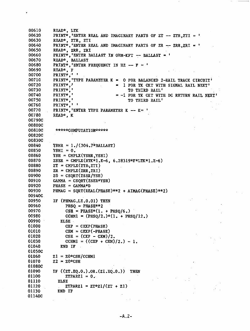
00610 READ*, LTK00620 PRINT*,'ENTER REAL AND IMAGINARY PARTS OF ZT — ZTR.ZTI — I00630 READ*, ZTR, ZTI00640 PRINT*,'ENTER REAL AND IMAGINARY PARTS OF ZR — ZRR,ZRI = 100650 READ*, ZRR, ZRI00660 PRINT*,'ENTER BALLAST IN OHM-KFT — BALLAST = '00670 READ*, BALLAST00680 PRINT*,'ENTER FREQUENCY IN HZ — F = '00690 READ*, F00700 PRINT*/' '00710 PRINT*,'TYPE PARAMETER K = 0 FOR BALANCED 2-RAIL TRACK CIRCUIT'00720 PRINT*,J = 1 FOR TK CKT WITH SIGNAL RAIL NEXT'00730 PRINT*\' TO THIRD RAIL'00740 PRINT*,' = -1 FOR TK CKT WITH DC RETURN RAIL NEXT00750 PRINT*,' TO THIRD RAIL'00760 PRINT*,' '00770 PRINT*,'ENTER TYPE PARAMETER K — K= '0078000790C00800C

READ*, K

00810C *****COMPUTATION*****00820C00830C

YSHR = l./(304.7^BALLAST)0084000850 YSHI = 0.00860 YSH = CMPLX(YSHR,YSHI)00870 ZSER = CMPLX(RTK*l.E-6, 6.28319*F*LTK*1.E-6)00880 ZT = CMPLX (ZTR-, ZTI)00890 ZR = CMPLX(ZRR,ZRI)00900 ZO = CSQRT(ZSER/YSH)00910 GAMMA = CSQRT(ZSER*YSH)00920 PHASE = GAMMA*D00930 PHMAG = SQRT(REAL(PHASE)**2 + AIMAG(PHASE)**2)00940C00950 IF (PHMAG.LE.0.01) THEN00960 PHSQ = PHASE**200970 CSH = PHASE*(1. + PHSQ/6.)00980 CCHMl = (PHSQ/2.)*(1. + PHSQ/12.)00990 ELSE01000 CXP = CEXP(PHASE)01010 CXM = CEXP(-PHASE)01020 CSH = (CXP - CXM)/2.01030 CCHMl = ((CXP + CXM)/2.) - 1.0104001050C

END IF01060 Zl = Z0*CSH/CCHM10107001080C

Z2 = Z0*CSH01090 IF ((ZT.EQ.O.).OR.(Zl.EQ.O.)) THEN01100 ZTPARZ1 =0.OHIO ELSE01120 ZTPARZ1 = ZT*Z1/(ZT + Zl)01130 END IF01140C ’

01150 IF ((ZR.EQ.O).OR.(Zl.EQ.O)) THEN01160 ZRPARZ1 = 0.01170 ELSE01180 ZRPARZ1 = ZR*Zl/(ZR + Zl)01190 END IF01200C01210 YPRIME = (Z1/(Z1 + ZR))/(ZTPARZ1 + Z2 + ZRPARZ1)01220 S = CMPLX(0., 2.*3.14159*F)01230 AK = REAL(K)01240 HCOND = YPRIME*(S*M3RR*1.E-6 + (AK*ZSER/2.))*CSH/GAMMA01250 HCONDR = REAL(HCOND)01260 HCONDI = AIMAG(HCOND)01270 HCONDM = SQRT(HC0NDR**2 + HCONDI**2)01280 HCONDPH = ATAN(HCONDl/HCONDR)*180./3.1415901290C01300C01310C *****data output*****01320C01330C01340 PRINT* 'A***********************************************************01350 PRINT*,' '01360 PRINT*,' *****inPUT DATA*****'01370 PRINT*,' '01380 PRINT 11, D, F, K01390 11 FORMAT(IX,'D = ',G11.4,' M, F = ',Gll.4,' HZ, K = ',12)01400 PRINT*,' '01410 PRINT 12, M3RR01420 12 FORMAT(IX,'M3RR = ',G11.4,' UH/M')01430 PRINT 13, ZSER01440 13 FORMAT(IX,'ZSER = ',G11.4,' + J(',G11.4,') OHMS/M')01450 PRINT 14, LTK01460 14 FORMAT(IX,'LTK - ' , Gll.4,' UH/M')01470 PRINT 15, ZT01480 15 F0RMAT(1X,'ZT = ',G11.4,' + J(',G11.4,') OHMS')01490 PRINT 16, ZR01500 16 FORMAT(IX,'ZR = ',G11.4,' + J(',Gll.4,') OHMS')01510 PRINT 17, BALLAST, YSHR01520 17 FORMAT(IX,'BALLAST = ',Gll.4,'KHOM-FT, YSHR =',Gll.4,'MHOS/M101530 PRINT* '***********************************************************•01540 PRINT*,' '01550 PRINT*,' *****0UTPUT DATA***** 101560 PRINT*,' '01570 PRINT 18, PHASE01580 18 FORMAT(IX,'GAMMA*D = ',G11.4,' + J(',Gll.4,')')01590 PRINT 19, ZO01600 19 FORMAT(IX,'ZO = ',G11.4,' + J(',Gll.4,') OHMS')01610 PRINT 21, Zl01620 21 F0RMAT(1X,'Z1 = '.Gll.4,' + J(',Gll.4,') OHMS')01630 PRINT 22, Z201640 22 F0RMAT(1X,'Z2 =',G11.4,' + J(>,611.4,') OHMS')01650 PRINT 23, HCOND01660 23 FORMAT(IX,'HCOND = ',Gll.4,' + J(',Gll.4,1)')01670 PRINT 24, HCONDM, HCONDPH01680 24 FORMAT(IX,' =',G11.4,' AT ',Gll.4,' DEGREES')

01690 PRINT*,'************************************************************•01700 PRINT*,' '01710 PRINT*,' '01720C01730C *****PROGRAM WILL NOW LOOP TO REPEAT FOR NEW DATA*****01740 GO TO 5001750C01760 END IF 01770C01780C *****THIS ENDS THE MAIN IF BLOCK*****01790C01800 PRINT*,'********************************************************'01810 PRINT*,' '01820 PRINT*,' COMPUTATION SESSION CLOSED. ADIOS, AMIGO.'01830 PRINT*,' '01840 PRINT*,' ******************************************************** •01850 END

REFERENCES

1. E. Holland-Moritz, "Electrical Parameters of Rail in Track Configuration," Final Report, U/M Project 32087, Dec. 1979, Cooley Electronics laboratory, Department of Electrical & Computer Engineering, University of Michigan.

2. A.E. Kennelly, F.H. Achard, & A.S. Dana, "Experimental researches on the skin effect in steel rails," J. Franklin Institute, Vol. 182, No. 2, Aug. 1916, pp. 135-189.

3. S. Ramo & J.R. Whinnery, Fields & Waves in Modern Radio, 2nd Edition, Wiley, New York, 1953, Table 9.01.

4. W.C. Johnson, Transmission Lines & Networks, McGraw-Hill, New York, 1950, Sec. 4.8.

5. A.J. Carey, "Basic track circuit limitations," Union Switch & Signal Div., American Standard, Inc., Swissvale, PA.

6. Ramo & Whinnery, op. cit., Chapter 6.

7. K. Frielinghaus, GRS, Inc., Rochester, N.Y., private communication.

8. J. Hoelscher & R. Rudich, "Compatibility of rate-coded audio-frequency track circuits with chopper propulsion drive in transit systems, Proceedings of the International Conference on Railways in the Electronic Age, sponsored by I.E.E., London, England, Nov. 17-20 1981, pp. 128-135.

9. J.F. Krempasky, G.E. Clark & L.A. Frasco, "EMI/EMC Rail Testing Program at WMATA,J' presented at the American Public Transit Association Rapid Transit Conference, Cleveland, Ohio, June 1982.

-R.l-

10. W.M. Truman, "Analysis, Measurement & Design to Assure Compatibility of Westinghouse Chopper Propulsion System and Union Switch & Signal Audio Frequency Track Circuits," presented at the American Public Transit Association Rapid Transit Conference, Cleveland, Ohio, June 1982.

11. E. Parzen, Modern Probability Theory and its Applications, Wiley, N.Y., 1960.

12. "Conductive Interference in Rapid Transit Signaling Systems - Volume II:Test Procedures," Report No. UMTA-MA-06-0153-85-6, to be published. See also preliminary reports: "Recommended practices for rail transit intrasystem electromagnetic compatibility of vehicular electrical power and track ciruit signaling subsystems." Vol. I: Inductive recommendedpractices. Vol. II: Conductive recommended practices. Rept. No.D0T-TSC-UM204-PM-82-21,I,II, Transportation Systems Center, Research & Special Programs Administration, U.S. Dept, of Transportation, Cambridge, MA 02142.

13. V. Nene, "Harmonic Characteristics of Rectifier Substations and Their Impact on Audio Frequency Track Circuits," U.S. Dept, of Transportation Report No. UMTA-MA-06-0025-81-6, May 1982.

14. T.J. Lowe & B. Melitt, "Thyristor chopper control and the introduction of harmonic current into track circuits," Proc; I,E.E., Vol. 121, No. 4, April 1974, pp. 269-275.

15. V. Nene, Advanced Propulsion Systems for Urban Rail Vehicles, Prentice- Hall, Englewood Cliffs, N.J., 1985.

☆ U. S. GOVERNMENT PRINTING OFFICE: 1 985 — 60O-hit — 20,153

218 copies -K.2-

U.S Department of TransportationResearch and Special Programs AdministrationKendall SquareCambridge. Massachusetts 02142

Official Business Penalty for Private Use $300

Postage and Fees Paid Research and Special Programs Administration DOT 513

UMTA Technical Assistance Program

Documents

Transcript of UMTA Technical Assistance Program