Technical Assistance Consultant's Report - 42384-012 ...

Technical Assistance Consultant’s Report

Project No. 42384-012October 2020

Knowledge and Innovation Support forADB's Water Financing Program

India: Water Productivity Measurement-Karnataka Integrated Sustainable Water Resouces Management Investment Program Tranche 2

Prepared by Karimi, P. and Pareeth, S.

IHE Delft Institute for Water Education, The Netherlands

For Asian Development Bank

This consultant’s report does not necessarily reflect the views of ADB or the Government concerned, and ADB and the Government cannot be held liable for its contents. (For project preparatory technical assistance: All the views expressed herein may not be incorporated into the proposed project’s design.

Remote Sensing Based Water Productivity Assessment – NLBC, Karnataka, India

FINAL REPORT

Project final report submitted to the Asian Development Bank under the program for Expanding

Support to Water Accounting in River Basins and Water Productivity in Irrigation Schemes.

Citation: Karimi, P., Pareeth, S. 2020. Remote Sensing Based Water Productivity Assessment – NLBC,

Karnataka, India. Project report, IHE Delft Institute for Water Education, The Netherlands.

Cover Image: Farmers in Karnataka. ACIWRM

i

EXPANDING SUPPORT TO WATER ACCOUNTING IN RIVER BASINS AND WATER PRODUCTIVITY IN IRRIGATION SCHEMES

Project final report:

Remote Sensing Based Water Productivity Assessment, NLBC,

Karnataka, India

PREPARED FOR THE ASIAN DEVELOPMENT BANK

BY

IHE Delft Institute for Water Education

October 2020

ii

Table of Contents

Table of Contents ii

List of abbreviations iii

List of Figures iv

List of Tables v

I. Introduction 1

A. WP activities in Karnataka 1

II. Implementation of Water Productivity activities 3

A. Study Area description 3

B. Summary of the approach 6

1. Data 6

2. Methodology 7

C. Results 14

1. Crop type mapping 14

2. Seasonal ETa, NDVI, AGBP, and WP in the NLBC 17

3. Crop based analysis for Kharif 2019 24

D. Key findings 34

E. References 36

III. Annexes 38

Annex 1. Cropping calendar in NLBC 38

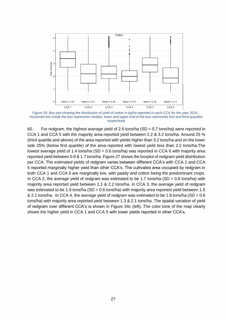
Annex 2. Agro-Climatic details of NLBC 39

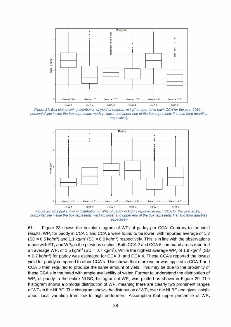
Annex 3. Hydro-Meteorological data 44

Annex 4. Landsat 8 and Sentinel 2A/B spectral bands 44

iii

List of abbreviations

ACIWRM Advanced Centre for Integrated Water Resources Management

ADB Asian Development Bank

AGBP Above Ground Biomass Production

CART CCA

Classification and Regression Trees Culturable Command Area

DN Digital Number

ETa Actual Evapotranspiration

ETx Maximum Crop Evapotranspiration

FAO Food and Agriculture Organization

GEE Google Earth Engine

GLDAS Global Land Data Assimilation System

GRD Ground Range Detected

GUI Graphical User Interface

HI Harvest Index

HPC High Performance Computing

IHE Delft IHE Delft Institute for Water Education

IWMI International Water Management Institute

LWR Locally Weighted Regression

ML Machine Learning

MODIS Moderate Resolution Imaging Spectroradiometer

NRSC National Remote Sensing Centre

NASA National Aeronautics and Space Administration

NDVI Normalized difference vegetation index

NLBC Narayanpur Left Bank Canal

ODK Open Data Kit

PySEBAL Python implementation of SEBAL

QA Quality Assessment

Rh Relative Humidity

Rn Net Radiation

RS Remote Sensing

RWD Relative Water Deficit

SAR Synthetic Aperture Radar

SD Standard Deviation

SEBAL Surface Energy Balance Model

SRTM Shuttle Radar Topography Mission

SWIR Short Wave Infra-red

TA Technical Assistance

TOA Top of Atmosphere

USGS The United States Geological Survey

WP Water Productivity

WPb Biomass Water Productivity

WPy Yield Water Productivity

iv

List of Figures

Figure 1:Conceptual framework of training proposed in the project with listed learning objectives

.................................................................................................................................................. 3

Figure 2: Study area map; Left – red box in the inset map shows the location of NLBC command

area in the state of Karnataka; Right – NLBC command boundaries with major rivers ............... 3

Figure 3: Schematic view of the NLBC canal network and CCA’s .............................................. 4

Figure 4: Cropping seasons in NLBC ......................................................................................... 5

Figure 5: Long-term monthly variation of minimum, maximum and average temperature over

NLBC ......................................................................................................................................... 5

Figure 6: Landsat tiles, processing units (PU) and elevation range over the NLBC .................... 6

Figure 7: NRSC Land use map at 60 m for the crop year 2017-18 and 2018-19 covering NLBC 7

Figure 8: ODK GUI in Quick mode (left) and Normal mode (right) .............................................. 8

Figure 9: Pictures taken during the field survey in Kharif 2019 ................................................... 9

Figure 10: a) False color composite of Sentinel 2 data from December 2019 with Paddy and

Cotton area, b) change in spectral reflectance over Sentinel 2 bands for a single paddy and cotton

point, c) NDVI change over growing period in 2019 of single paddy and cotton points ..............10

Figure 11: The PySEBAL methodological framework for WP assessment ................................11

Figure 12: Field data collected from NLBC in 2019 ...................................................................14

Figure 13: Crop type map developed using ML for the 2019 Kharif season ...............................15

Figure 14: Percentage crop area distribution in all the CCA’s for the year 2019 represented as a

stacked bar chart ......................................................................................................................16

Figure 15: Error matrix of ML-based crop type classification for the 2019 Kharif season ...........17

Figure 16: Seasonal ETa maps of Kharif 2017, 2018, and 2019 in the NLBC ...........................18

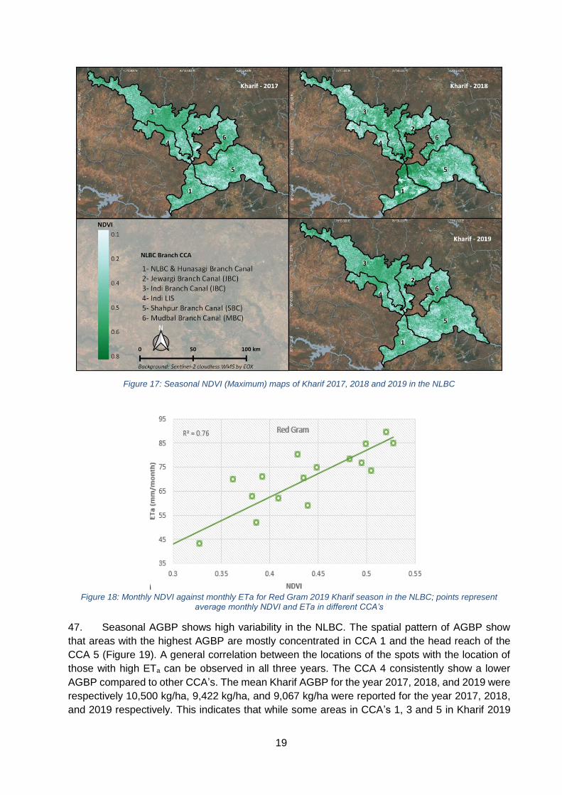
Figure 17: Seasonal NDVI (Maximum) maps of Kharif 2017, 2018 and 2019 in the NLBC ........19

Figure 18: Monthly NDVI against monthly ETa for Red Gram 2019 Kharif season in the NLBC;

points represent average monthly NDVI and ETa in different CCA’s .........................................19

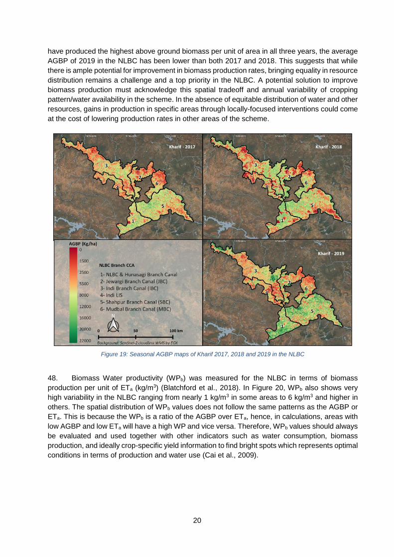
Figure 19: Seasonal AGBP maps of Kharif 2017, 2018 and 2019 in the NLBC .........................20

Figure 20: Seasonal WP maps of Kharif 2017, 2018 and 2019 in the NLBC .............................21

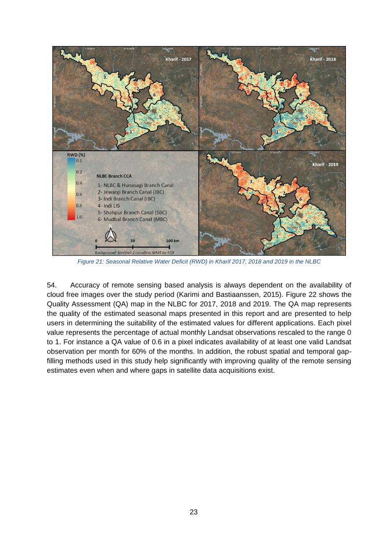
Figure 21: Seasonal Relative Water Deficit (RWD) in Kharif 2017, 2018 and 2019 in the NLBC

.................................................................................................................................................23

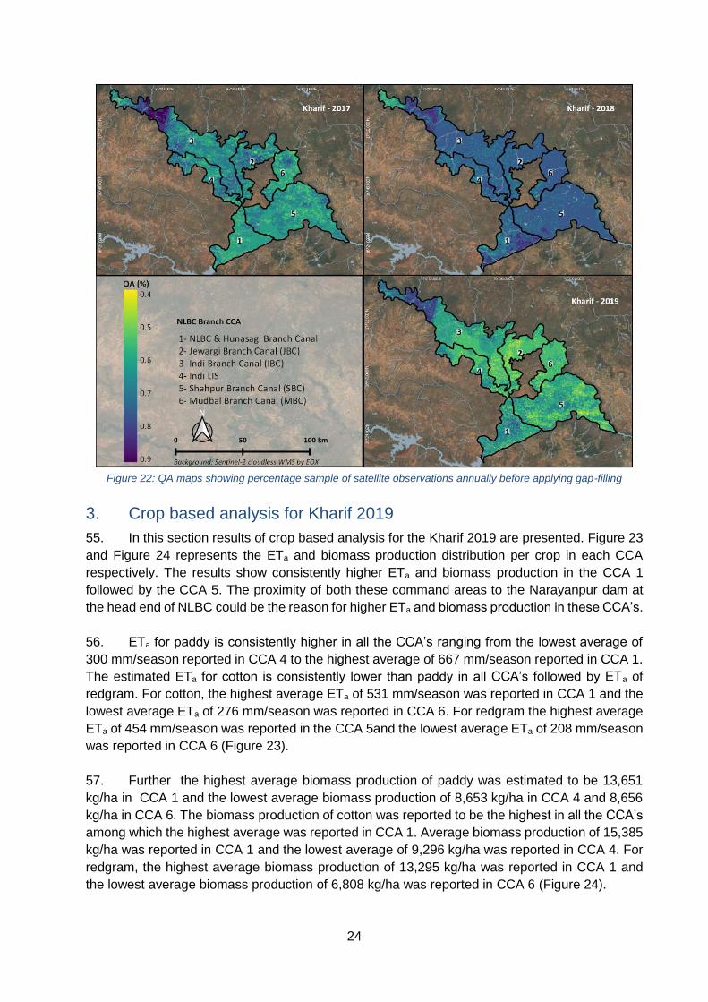
Figure 22: QA maps showing percentage sample of satellite observations annually before

applying gap-filling ....................................................................................................................24

Figure 23: Bar chart showing average ETa in mm/season per crop reported in each CCA for the

year 2019 ..................................................................................................................................25

Figure 24: Bar chart showing average AGBP in kg/ha per crop reported in each CCA for the year

2019 ..........................................................................................................................................25

Figure 25: Box plot showing the distribution of yield of paddy in kg/ha reported in each CCA for

the year 2019, horizontal line inside the box represents median; lower and upper end of the box

represents first and third quartiles respectively..........................................................................26

Figure 26: Box plot showing the distribution of yield of cotton in kg/ha reported in each CCA for

the year 2019, , horizontal line inside the box represents median; lower and upper end of the box


Figure 27: Box plot showing distribution of yield of redgram in kg/ha reported in each CCA for the

year 2019, , horizontal line inside the box represents median; lower and upper end of the box


v

Figure 28: Box plot showing distribution of WPy of paddy in kg/m3 reported in each CCA for the



Figure 29: Histogram showing distribution of WPy of paddy in kg/m3 over entire NLBC for the

year 2019 ..................................................................................................................................29

Figure 30: Box plot showing distribution of WPy of cotton in kg/m3 reported in each CCA for the



Figure 31: Histogram showing distribution of WPy of cotton in kg/m3 over entire NLBC for the

year 2019 ..................................................................................................................................30

Figure 32: Box plot showing distribution of WPy of redgram in kg/m3 reported in each CCA for

the year 2019, , horizontal line inside the box represents median; lower and upper end of the box


Figure 33: Histogram showing distribution of WPy of redgram in kg/m3 over entire NLBC for the

year 2019 ..................................................................................................................................31

Figure 34: Yield (left) and WPy (right) maps of a) Paddy, b) Cotton and c) Redgram for the year

2019 ..........................................................................................................................................32

List of Tables

Table 1: CCA supported by branch canals in NLBC ................................................................... 4

Table 2: Meteorological data and its units used for the PySEBAL model.................................... 7

Table 3: HI and MOI values used in computing yield per crop ...................................................13

Table 4: Comparison of RS and field-based yield estimates per crop for the year 2019 ............13

Table 5: Number of training and validation points per crop type for the ML model .....................14

Table 6: Area (ha) covered by different cropping seasons in NLBC for two crop years .............16

Table 7: Area (ha) covered by Kharif crops in 2017-18 and 2018-19 per each branch CCA ......16

Table 8: Area (ha) covered by major crops in 2019 Kharif season per each branch CCA .........17

Table 9: Mean ETa, AGBP and WPb for different branch CCA’s in 2019 Kharif season ............21

Table 10: Area of bright spots per crop in each CCA, the threshold values used to compute the

bright spots are also listed ........................................................................................................33

1

I. Introduction

1. The Asian Development Bank (ADB) is committed under its Water Operational Plan 2011-

2020 to undertake expanded and enhanced analytical work to enable its developing member

countries to secure a deeper and sharper understanding of water issues and solutions. IHE Delft,

in collaboration with the International Water Management Institute (IWMI) and the Food and

Agricultural Organization of the United Nations (FAO), supports ADB in achieving this objective.

2. The activities proposed for the current Technical Assistance (TA) build on the work

previously undertaken by IHE Delft in cooperation with the ADB to assess crop water productivity

and to assess water resource status in selected basins/countries in Asia. Toward this, IHE Delft

in coordination with local partners is deploying remote sensing based Water Productivity (WP)

assessment to quantify the crop yield harvested per unit of consumed net water. Remote sensing

(RS) based assessment of WP is based on actual evapotranspiration (ETa) to estimate net water

consumption. We use the in-house developed PySEBAL model to compute ETa and Above

Ground Biomass Production (AGBP) at 30 m spatial resolution over multiple cropping seasons.

3. This project aimed to contribute to sustainable development in Asia’s irrigation sector, and

to create more value from scarce water resources. India is one of the 5 countries where advanced

technologies to measure WP from satellite data were introduced. The current project funded by

ADB aims to study water productivity and perform water accounting in the Krishna basin. The

Krishna basin is an interstate river system that flows through Maharashtra (26% of the area),

Karnataka (44%), and Andhra Pradesh (30%). The majority of the Krishna basin about 76% is

covered by agricultural area. Irrigated areas have expanded rapidly in the past 50 years causing

a significant decrease in discharge to the sea. The Krishna basin is facing growing challenges in

satisfying the growing water demands and conflicts are arising because of competing demands.

The overall aim of the water productivity study in Karnataka is to do a water productivity

assessment by expanding the methodology used in Phase-I for Tungabhadra Left Bank

Command (TLBC) to a new area and provide detailed analysis. The work is been carried out in

coordination with the Advanced Centre for Integrated Water Resources Management (ACIWRM).

This midterm report explains the ongoing activities with preliminary results of the WP assessment

of a selected irrigation scheme in Karnataka, India.

A. WP activities in Karnataka

4. The WP activities in Karnataka were decided during the inception workshop conducted

from July 29 – August 2, 2019 in Belgaum, Karnataka hosted by Visvesvaraya Technological

University. Three major activities with several milestones and deliverables were fixed. The

activities with deliverables are:

- Remote sensing based WP assessment

- Fieldwork

- Capacity building

5. The activities are elaborated in the following sections.

2

I. Remote sensing based WP assessment

6. The ACIWRM is interested in the three command areas in K2, K3, and K4 sub-basins of

the Krishna basin. Given the project timelines and resources, it was agreed that IHE Delft would

provide a detailed water productivity assessment in one of the three irrigation schemes located in

these sub-basins. The focus scheme was decided to be Narayanpur Left Bank Canal (NLBC)

command area by the ACIWRM considering the local priorities. The agreed deliverables for the

focus scheme are:

1- Evapotranspiration maps at 30 meter resolution

2- Biomass production maps at 30 meter resolution

3- Crop map for major crop(s) - 2019

4- Yield maps at 30 meter resolution for the selected major crops

5- Crop water productivity maps at 30 meter resolution

6- A final report describing the results and interpretations of the outputs

7. The study was carried out for the Kharif seasons in three years from 2017 to 2019. Kharif

season starts in July till December/January. The main crops cultivated include sugarcane, cotton,

paddy, sorghum, beans, and maize, among others. The cropping pattern differs in different

schemes in the Krishna basin (Annex 1 list the cropping calendar of major crops in NLBC).

II. Fieldwork

8. ACIWRM experts were trained on the subject of ground data collection using mobile

devices and Open Data Kit (ODK) tool during the Phase-I of the project. Phase-II capitalized on

this existing capacity and the ground data collection campaign was led by the local experts from

ACIWRM under the supervision of IHE Delft experts. The field data collection was carried out in

the NLBC scheme in December 2019 and January 2020.

III. Capacity building

9. Capacity building is an important pillar of the project. To fulfill the capacity building

requirement in water productivity assessment, IHE Delft carried out two training workshops with

a follow-up day-session during the final workshop of the project. The first training was conducted

in Belguam, Karnataka from 29th July to August 2nd, 2019. The second training was conducted

from March 3rd to 6th 2020. The third training was conducted online from July 28th to 30th 2020.

The participants in the training received hands-on assignments after finishing each training. This

is to encourage the participants to use what they learned in real case applications. The

assignment is being carried out by the participants in groups (3-4 members) and they work on

preparing remote sensing based WP assessment for different selected (sub) schemes in the study

area. The participants had access to resource persons from IHE Delft via email and periodical

skype sessions (every 3 weeks). The ACIWRM coordinated the formation of the working groups

and taken initiative in scheduling the remote consultation sessions. The same assignment was

carried forward to the second training, where trainees learned how to implement the gap-filling

techniques to the processed data. Figure 1 shows the conceptual framework of the proposed

training, their learning objectives, and the target output.

3

Figure 1:Conceptual framework of training proposed in the project with listed learning objectives

II. Implementation of Water Productivity activities

A. Study Area description

10. The WP studies were carried out in the Narayanpur Left Bank Canal (NLBC) command

area under the Upper Krishna Project (UKP) in Northern Karnataka state in India (Wallach, 1984).

This study focus on the NLBC network which comprises an irrigated area of 451,703 ha as per

the official statistics. The NLBC is divided into six culturable command areas (CCA’s) that are

supported by the branch canals (Figure 2). These include NLBC/Hunasagi Branch Canal (CCA

1), Jewargi Branch Canal (CCA 2), Indi Branch Canal (CCA 3), Indi Lift Irrigation Scheme (CCA

4), Shahpur Branch Canal (CCA 5), and Mudbal Branch Canal (CCA 6). Hereafter in this report,

the larger scheme is termed as NLBC and numbers are used to identify CCA’s.

Figure 2: Study area map; Left – red box in the inset map shows the location of NLBC command area in the state of

Karnataka; Right – NLBC command boundaries with major rivers

11. The canals were constructed between 1982 and 1997 and since then used for irrigation

purposes. Official CCA’s areas are listed in Table 1 (based on: KJBNL, 2012). The Indi branch

canal is the biggest CCA with an area of 131,260 ha and Indi LIS the smallest with an area of

43,000 ha.

4

Table 1: CCA supported by branch canals in NLBC

CCA No.

Canal Command area in ha

1 NLBC & Hunasagi Branch Canal 47,223

2 Jewargi Branch Canal 57,100

3 Indi Branch Canal 131,260

4 Indi Lift Irrigation Scheme 43,000

5 Shahapur Branch Canal 122,120

6 Mudbal Branch Canal 51,000

Total 451,703

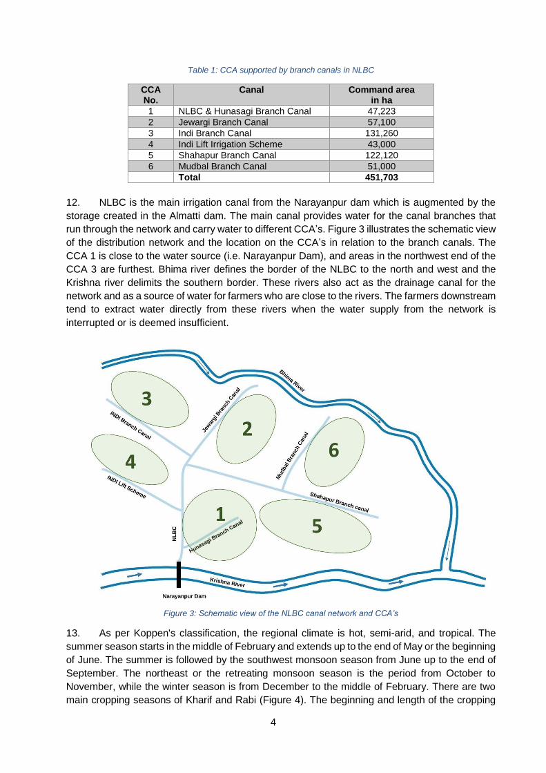
12. NLBC is the main irrigation canal from the Narayanpur dam which is augmented by the

storage created in the Almatti dam. The main canal provides water for the canal branches that

run through the network and carry water to different CCA’s. Figure 3 illustrates the schematic view

of the distribution network and the location on the CCA’s in relation to the branch canals. The

CCA 1 is close to the water source (i.e. Narayanpur Dam), and areas in the northwest end of the

CCA 3 are furthest. Bhima river defines the border of the NLBC to the north and west and the

Krishna river delimits the southern border. These rivers also act as the drainage canal for the

network and as a source of water for farmers who are close to the rivers. The farmers downstream

tend to extract water directly from these rivers when the water supply from the network is

interrupted or is deemed insufficient.

Figure 3: Schematic view of the NLBC canal network and CCA’s

13. As per Koppen's classification, the regional climate is hot, semi-arid, and tropical. The

summer season starts in the middle of February and extends up to the end of May or the beginning

of June. The summer is followed by the southwest monsoon season from June up to the end of

September. The northeast or the retreating monsoon season is the period from October to

November, while the winter season is from December to the middle of February. There are two

main cropping seasons of Kharif and Rabi (Figure 4). The beginning and length of the cropping

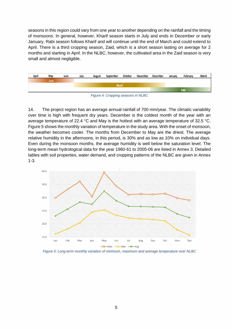
5

seasons in this region could vary from one year to another depending on the rainfall and the timing

of monsoons. In general, however, Kharif season starts in July and ends in December or early

January. Rabi season follows Kharif and will continue until the end of March and could extend to

April. There is a third cropping season, Zaid, which is a short season lasting on average for 2

months and starting in April. In the NLBC, however, the cultivated area in the Zaid season is very

small and almost negligible.

Figure 4: Cropping seasons in NLBC

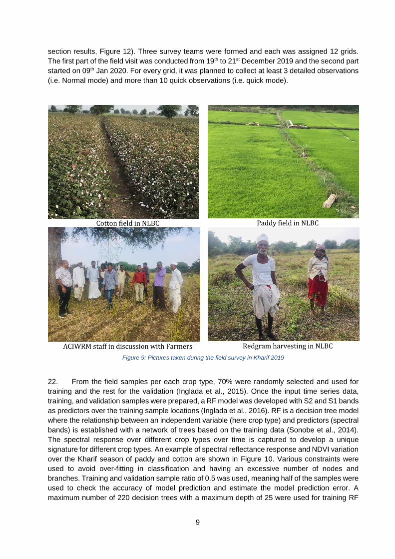
14. The project region has an average annual rainfall of 700 mm/year. The climatic variability

over time is high with frequent dry years. December is the coldest month of the year with an

average temperature of 22.4 °C and May is the hottest with an average temperature of 32.5 °C.

Figure 5 shows the monthly variation of temperature in the study area. With the onset of monsoon,

the weather becomes cooler. The months from December to May are the driest. The average

relative humidity in the afternoons, in this period, is 30% and as low as 10% on individual days.

Even during the monsoon months, the average humidity is well below the saturation level. The

long-term mean hydrological data for the year 1960-61 to 2005-06 are listed in Annex 3. Detailed

tables with soil properties, water demand, and cropping patterns of the NLBC are given in Annex

1-3.

Figure 5: Long-term monthly variation of minimum, maximum and average temperature over NLBC

6

B. Summary of the approach

1. Data

15. All the Landsat 8 data acquired between 1 January 2017 and 31 December 2019 were

processed to estimate ETa and AGBP. The entire NLBC is covered in 3 Landsat tiles. This

includes two tiles from path 145 and a single tile from path 146 (Figure 6). A total of 156 Landsat

8 scenes were processed. Although the target season of the study is Kharif which is from July to

December, we processed all the images from 1 January 2017 to 31 December 2019 to provide

the continuity in the temporal moving window over months/seasons for the gap-filling step that

comes at a later stage. All the spectral bands including the thermal bands were processed in

preparation to apply the SEBAL algorithm. The Landsat data preprocessing was performed at a

spatial resolution of 30 m, resulting in a total of 7.5 million pixels for each map covering the entire

NLBC. A total of 312 maps each with 7.5 million pixels were processed, 2.3 billion pixel-date, to

develop seasonal ETa and Biomass maps. We used the Landsat Collection 1 Level-1 data

belonging to the Tier 1(T1) inventory. For topography and elevation, 30 m data from NASA’s

Shuttle Radar Topography Mission (SRTM), acquired from USGS EROS Data Center was used.

All the Landsat data were downloaded from Google cloud public storage. The data acquisition

was automated using the gsutil open-source python library

(https://github.com/GoogleCloudPlatform/gsutil/).

Figure 6: Landsat tiles, processing units (PU) and elevation range over the NLBC

https://github.com/GoogleCloudPlatform/gsutil/

7

16. For setting up the PySEBAL model, meteorological data at the time of satellite data

acquisition (instantaneous) and 24-hour average representing the day of acquisition are required.

The meteorological data required are listed in Table 2. These data were extracted for the NLBC

area from NASA Global Land Data Assimilation System (GLDAS v2.1) which is an assimilated

global data product from satellite and ground-based observations. GLDAS data is offered at 0.25-

degree spatial resolution at 3 hours interval.

Table 2: Meteorological data and its units used for the PySEBAL model

Parameter Symbols Unit

Downward shortwave

radiation

SWdown W/m2

Wind speed Ws m/s

Air temperature Tair °C

Pressure P Mb

Relative humidity Rh %

17. The latest available land use maps for two crop years 2017-18 and 2018-19 were obtained

from the National Remote Sensing Centre (NRSC). The NRSC map is of 60 m spatial resolution

and classifies 17 land use types for the 2017-18 cropping year (Figure 7). This map was used to

inform the crop type mapping process in the project.

18. For crop type mapping for the year 2019, the Sentinel 2A/B multi-spectral and Sentinel 1

Synthetic Aperture Radar (SAR) data available from July 2019 to January 2020 were used. Due

to the extensive cloud coverage during the period, we could only use atmospherically corrected

Sentinel 2 data from November 2020 and January 2021 for the crop type mapping. Further,

Sentinel 1 SAR data, a median filter was applied per month to create a monthly time series from

July 2019 to January 2020. The entire crop type mapping was implemented in Google Earth

Engine (GEE).

Figure 7: NRSC Land use map at 60 m for the crop year 2017-18 and 2018-19 covering NLBC

2. Methodology

Mapping Crop types

8

19. The crop type mapping was implemented using Machine Learning (ML). The Random

Forest (RF) algorithm was applied to the time series of Sentinel 1 and cloud-free Sentinel 2A/B

scenes available in the GEE platform (Gorelick et al., 2017). The preprocessed Sentinel 1 SAR

Ground Range Detected (GRD) data in dual-band cross-polarization, vertical transmit/horizontal

receive (VH) at 10 m spatial resolution was used for the classification. A median filter was applied

on monthly S1 GRD scenes to create monthly time series from July 2019 to January 2020. A time

series of S2 bands (2,3,4,5,6,7,8,8A,11,12) and S1 monthly median VH bands were created for

the NLBC region to apply the ML algorithm for crop type classification (Pareeth et al., 2019).

Spectral bands of S2 data are provided in Annex 4.

20. Fieldwork was carried out in December 2019 and January 2020 to take sample points

representing different crop types in the study area. This fieldwork aimed to support the crop type

mapping and to enhance the understanding of the agricultural practices. Open Data Kit (ODK)

platform was used during the survey. ODK was configured by the ACIWRM and the questionaries’

were finalized in consultation with IHE Delft experts. Figure 8 shows the Graphical User Interface

(GUI) of the ODK app developed in quick and normal mode. The quick mode captured the latitude

& longitude details of the field and crop type. The normal mode had detailed questions and

required interacting with farmers to collect data on fertilizer applications, seed types and rates,

and yield details (Figure 9).

Figure 8: ODK GUI in Quick mode (left) and Normal mode (right)

21. To achieve a uniform distribution of samples in the NLBC command area, the command

area was divided into grids of 15 km (Foody, 2002). 36 grids covered the command area (see

9

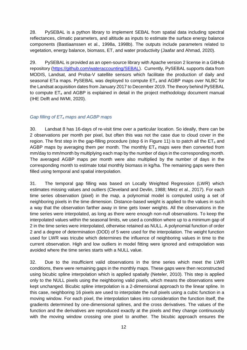
section results, Figure 12). Three survey teams were formed and each was assigned 12 grids.

The first part of the field visit was conducted from 19th to 21st December 2019 and the second part

started on 09th Jan 2020. For every grid, it was planned to collect at least 3 detailed observations

(i.e. Normal mode) and more than 10 quick observations (i.e. quick mode).

Cotton field in NLBC

Paddy field in NLBC

ACIWRM staff in discussion with Farmers

Redgram harvesting in NLBC

Figure 9: Pictures taken during the field survey in Kharif 2019

22. From the field samples per each crop type, 70% were randomly selected and used for

training and the rest for the validation (Inglada et al., 2015). Once the input time series data,

training, and validation samples were prepared, a RF model was developed with S2 and S1 bands

as predictors over the training sample locations (Inglada et al., 2016). RF is a decision tree model

where the relationship between an independent variable (here crop type) and predictors (spectral

bands) is established with a network of trees based on the training data (Sonobe et al., 2014).

The spectral response over different crop types over time is captured to develop a unique

signature for different crop types. An example of spectral reflectance response and NDVI variation

over the Kharif season of paddy and cotton are shown in Figure 10. Various constraints were

used to avoid over-fitting in classification and having an excessive number of nodes and

branches. Training and validation sample ratio of 0.5 was used, meaning half of the samples were

used to check the accuracy of model prediction and estimate the model prediction error. A

maximum number of 220 decision trees with a maximum depth of 25 were used for training RF

10

model. Accuracy assessment following the standard approach of developing an error matrix using

validation samples was performed after classification (Foody, 2002).

23. Further 57 points were collected from the field with yield information of the crop grown.

Out of 57 points, 19 for cotton, 12 for paddy, and 11 for redgram. These points are used to validate

the RS based yield estimates by comparing the average yield from RS and field per crop.

Figure 10: a) False color composite of Sentinel 2 data from December 2019 with Paddy and Cotton area, b) change

in spectral reflectance over Sentinel 2 bands for a single paddy and cotton point, c) NDVI change over growing period in 2019 of single paddy and cotton points

Mapping Actual Evapotranspiration (ETa) and Above Ground Biomass Production (AGBP)

24. The acquired Landsat 8 data were pre-processed to create cloud masked Top Of

Atmosphere (TOA) reflectance bands. The pre-processing included conversion from Digital

Number (DN) to TOA reflectance, cloud removal using the Quality Assessment (QA) band

provided along with the data, and mosaicking the same path tiles. All the satellite data pre-

processing is done inside PySEBAL (Steps 1, 2 in Figure 11). The preprocessing of

meteorological data included the following steps: i) extract the variable and clip to study area, iii)

converting the units of air temperature from Kelvin to °C, pressure from Pascal (Pa) to Millibar

(mb), and specific humidity in kg/kg to relative humidity in % and iv) extracting instantaneous and

daily average meteorological variables from three-hourly data. The instantaneous data

corresponding to the Landsat acquisition time (10:30 A.M local time) was estimated by averaging

the 6H and 9H outputs from GLDAS, while all the 8 images in a day were averaged to estimate

24 hours data representing the day of Landsat acquisition.

11

Figure 11: The PySEBAL methodological framework for WP assessment

25. To efficiently process the Landsat data for a large area such as NLBC (~471,779 ha) the

entire processing chain was implemented in a supercomputing infrastructure. A High Performance

Computing (HPC) and cloud data infrastructure with Linux operating system was used to carry

out the entire workflow from data acquisition to gap-filling the ETa and AGBP outputs. We rented

a system and storage in HPC cloud infrastructure from a service provider called Hetzner. The

advantage is that we can setup and configure the system, including the processor, memory,

storage space etc. A Linux based environment with open source softwares was used, which

makes it more optimized and economical. The cost is around 5000 Euro per year for this setup.

But the cost will vary depending on the amount of data you want to process.There are major

players like Google cloud, Amazon AWS and Microsoft Azure, but comparatively on an expensive

side for the amount of data we want to process.

26. The entire processing chain was performed using multiple open-source libraries, for

handling multi-core jobs, processing satellite data, and implementing the PySEBAL model. HPC

cloud offers a dynamically scalable and fully configurable environment thereby ensuring the free

choice of tools by the user to deploy for specific tasks. All the spatial and temporal processing

were performed in GRASS GIS 7.8 software which is an open-source and available under GNU

General Public License (GPL).

27. The Landsat processing for each path (145, 146) was performed in different nodes in

parallel. This approach resulted in a substantial reduction in processing time. The data processing

was divided into two Processing Units (PU) based on the Landsat path and row. Since the

adjacent tiles in the same path have the same acquisition date, we chose each path as an

individual processing unit. Thus data for each path were processed in parallel in the HPC. Figure

6 shows the bounding box of the two defined PUs for NLBC. The PU’s are designed to incorporate

the minimum overlapping “rectangular” area between the respective Landsat path and the NLBC

area. While processing in each PU, only those pixels inside the NLBC were considered.

12

28. PySEBAL is a python library to implement SEBAL from spatial data including spectral

reflectances, climatic parameters, and altitude as inputs to estimate the surface energy balance

components (Bastiaanssen et al., 1998a, 1998b). The outputs include parameters related to

vegetation, energy balance, biomass, ET, and water productivity (Jaafar and Ahmad, 2020).

29. PySEBAL is provided as an open-source library with Apache version 2 license in a GitHub

repository (https://github.com/wateraccounting/SEBAL). Currently, PySEBAL supports data from

MODIS, Landsat, and Proba-V satellite sensors which facilitate the production of daily and

seasonal ETa maps. PySEBAL was deployed to compute ETa and AGBP maps over NLBC for

the Landsat acquisition dates from January 2017 to December 2019. The theory behind PySEBAL

to compute ETa and AGBP is explained in detail in the project methodology document manual

(IHE Delft and IWMI, 2020).

Gap filling of ETa maps and AGBP maps

30. Landsat 8 has 16-days of re-visit time over a particular location. So ideally, there can be

2 observations per month per pixel, but often this was not the case due to cloud cover in the

region. The first step in the gap-filling procedure (step 6 in Figure 11) is to patch all the ETa and

AGBP maps by averaging them per month. The monthly ETa maps were then converted from

mm/day to mm/month by multiplying each map by the number of days in the corresponding month.

The averaged AGBP maps per month were also multiplied by the number of days in the

corresponding month to estimate total monthly biomass in kg/ha. The remaining gaps were then

filled using temporal and spatial interpolation.

31. The temporal gap filling was based on Locally Weighted Regression (LWR) which

estimates missing values and outliers (Cleveland and Devlin, 1988; Metz et al., 2017). For each

time series observation (pixel) in the map, a polynomial model is computed using a set of

neighboring pixels in the time dimension. Distance-based weight is applied to the values in such

a way that the observation farther away in time gets lower weights. All the observations in the

time series were interpolated, as long as there were enough non-null observations. To keep the

interpolated values within the seasonal limits, we used a condition where up to a minimum gap of

2 in the time series were interpolated, otherwise retained as NULL. A polynomial function of order

2 and a degree of determination (DOD) of 5 were used for the interpolation. The weight function

used for LWR was tricube which determines the influence of neighboring values in time to the

current observation. High and low outliers in model fitting were ignored and extrapolation was

avoided where the time series starts with a NULL value.

32. Due to the insufficient valid observations in the time series which meet the LWR

conditions, there were remaining gaps in the monthly maps. These gaps were then reconstructed

using bicubic spline interpolation which is applied spatially (Neteler, 2010). This step is applied

only to the NULL pixels using the neighboring valid pixels, which means the observations were

kept unchanged. Bicubic spline interpolation is a 2-dimensional approach to the linear spline. In

this case, neighboring 16 pixels are used to interpolate the null pixels using a cubic function in a

moving window. For each pixel, the interpolation takes into consideration the function itself, the

gradients determined by one-dimensional splines, and the cross derivatives. The values of the

function and the derivatives are reproduced exactly at the pixels and they change continuously

with the moving window crossing one pixel to another. The bicubic approach ensures the

https://github.com/wateraccounting/SEBAL

13

continuation of derivatives to the adjacent grids thereby reducing the artifacts. After the gap-filling

process applied to all the monthly maps from January 2017 to December 2019, we aggregated

the monthly maps (July to December) to create Kharif seasonal maps.

Yield and CWP mapping for the year 2019

33. Following the seasonal mapping of ETa and AGBP, the yield of each of the major crops

as per crop type map of 2019 was derived. The crop yield was computed using the Harvest Index

(HI) of each of these crops following the literature and previous studies by IHE Delft. The HI and

moisture index used for computing the yield is given in Table 3. Yield is computed then using the

following equation:

𝑌𝑖𝑒𝑙𝑑 =𝐴𝐺𝐵𝑃 ∗ 𝐻𝐼

1 − 𝑀𝑂𝐼

34. Where yield is in kg/ha, AGBP is Above Ground Biomass Production in kg/ha, HI is

Harvest Index and MOI is moisture content of the crop.

35. Further crop water productivity is computed using the equation:

𝑊𝑃𝑦 =𝑌𝑖𝑒𝑙𝑑

𝐸𝑇𝑎

36. Where WPy water productivity is expressed in kg/m3, yield in kg/ha. ETa is actual

evapotranspiration converted into the volume of water per unit area in m3/ha.

Table 3: HI and MOI values used in computing yield per crop

HI MOI Reference

Paddy 0.47 0.12 Cai X, & Bastianssen

W, 2018

Cotton 0.21 0.02

Redgram 0.19* Sheldrake, A.R, & Narayanan A, 1976

* for Redgram the HI value used is for dry matter, hence MOI is ignored in the equation for WPy

37. The Table 4 lists the comparison of yield computed from field data and remote sensing

based estimates. As the number of points (57) were not enough to represent the entire NLBC a

comparison analysis was performed by taking average yield per crop from field and RS data. The

comparison shows that the RS based estimates are well aligned with the field estimates. Cotton

yields estimated from the field were found to be on a higher range compared to RS estimates

while yields of both paddy and redgram were found to be in the same range.

Table 4: Comparison of RS and field-based yield estimates per crop for the year 2019

Average Yield (tons/ha)

Crop type RS Field

Paddy 6.2 6.2

Cotton 2.6 3.3

Redgram 1.8 1.7

14

C. Results

38. The following subsections explain the results of remote sensing based water productivity

assessment in the NLBC. This report is adapted to the comments received from the stakeholders

on the mid-term report.

1. Crop type mapping

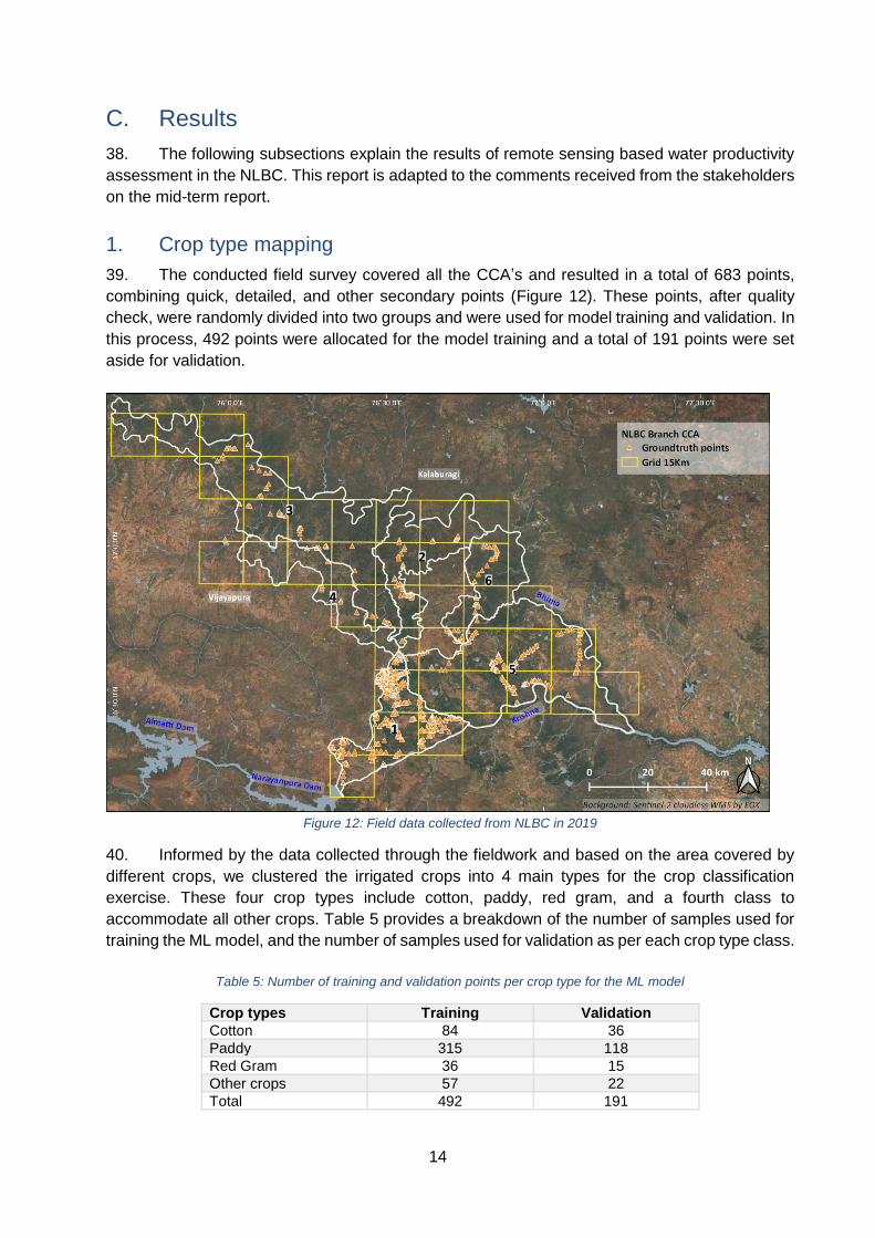
39. The conducted field survey covered all the CCA’s and resulted in a total of 683 points,

combining quick, detailed, and other secondary points (Figure 12). These points, after quality

check, were randomly divided into two groups and were used for model training and validation. In

this process, 492 points were allocated for the model training and a total of 191 points were set

aside for validation.

Figure 12: Field data collected from NLBC in 2019

40. Informed by the data collected through the fieldwork and based on the area covered by

different crops, we clustered the irrigated crops into 4 main types for the crop classification

exercise. These four crop types include cotton, paddy, red gram, and a fourth class to

accommodate all other crops. Table 5 provides a breakdown of the number of samples used for

training the ML model, and the number of samples used for validation as per each crop type class.

Table 5: Number of training and validation points per crop type for the ML model

Crop types Training Validation

Cotton 84 36

Paddy 315 118

Red Gram 36 15

Other crops 57 22

Total 492 191

15

41. Using the methodology explained in the previous chapter, a crop type map at 20 m spatial

resolution with 4 crop types – ‘Cotton’, ‘Paddy’, ‘Red gram’, and ‘Other crops’ was developed for

the Kharif season of 2019. The crop map depicts the spatial distribution of crops (Figure 13).

Broadly it can be seen that paddy cultivation, shown in light green, is mostly concentrated in areas

closer to the main water source. These areas include the majority of CCA 1 and parts of the CCA

2, 3, 4, 5, and 6 that are close to the main distribution canal at the head reach. While cotton

spreads in the middle reach of CCA’s, the red gram is mostly cultivated in the tail reach. The

observed spatial pattern in crop cultivation can be explained by the pattern of water availability

and water distribution from head to tail. Paddy, as the most water-consuming crop of the three, is

cultivated near the headworks and red gram which needs the least amount of water at the tail

where water availability is strained. Although this general pattern is, at some places, broken

because some farmers who are close to rivers, streams, and drainage canals tend to abstract

water directly from these sources to cultivate paddy. For example, paddy cultivation can be

detected in the map in areas along the banks of Bhima River in CCA 5.

Figure 13: Crop type map developed using ML for the 2019 Kharif season

42. Area statistics based on NRSC maps of two crop years are given in Table 6 & Table 7.

The cropping dynamics in the region change rapidly depending on the availability of the water

and rainfall patterns. Statistical analysis using the NRSC maps shows that the total area under

cultivation in Kharif 2017-18 and 2018-19 was 443,188 ha and 396,039 ha respectively. Kharif

2018 reported the lowest irrigated area, mainly contributed by lack of rainfall. The year 2018 was

reported with the lowest annual rainfall during kharif. The total rainfall during kharif was 550 mm,

321 mm, 506 mm for the years 2017, 2018 and 2019 respectively.

16

Table 6: Area (ha) covered by different cropping seasons in NLBC for two crop years

Class ID Class Name 2017-18 2018-19

1 Kharif Crop 197,774 237,116

2 Rabi Crop 53,768 28,114

3 Double/Triple Crop 245,414 158,923

4 Current Fallow 98,906 171,796

Total Kharif 443,188 396,039

Total Cropped area 496,956 424,153

Table 7: Area (ha) covered by Kharif crops in 2017-18 and 2018-19 per each branch CCA

CCA Name Kharif cropped area (2017-18)

Kharif cropped area (2018-19)

1 NLBC & Hunasagi Branch Canal 57411 56098

2 Jewargi Branch Canal (JBC) 52242 43527

3 Indi Branch Canal (IBC) 132036 127876

4 Indi Lift Irrigation Scheme 47404 28273

5 Shahpur Branch Canal (SBC) 118527 100245 6 Mudbal Branch Canal (MBC) 35567 40018

Total Kharif area in NLBC 443,188 396,039

43. In the 2019 Kharif season, major crop types in all the branch CCA’s are either Paddy,

Cotton, or Red Gram. In the CCA 1, the dominant crop is Paddy (70%) followed by Cotton (24%).

In the CCA 3 which is the largest CCA as per official statistics, both Paddy (39%) and Cotton

(37%) are dominantly cultivated followed by Red Gram (24%). In CCA 5, Cotton is dominant

covering 53% of CCA followed by Paddy (42%). In CCA 6 Cotton is widely cultivated with 63%

followed by Red Gram (24%) and Paddy (13%). Table 8 lists the area covered by major crops in

different CCA’s and Figure 14 shows the percentage of crop area distribution in all the CCA’s for

the year 2019.

Figure 14: Percentage crop area distribution in all the CCA’s for the year 2019 represented as a stacked bar chart

0%

10%

20%

30%

40%

50%

60%

70%

80%

90%

100%

Entire NLBC NLBC &HunasagiBranchCanal

JewargiBranch

Canal (JBC)

Indi BranchCanal (IBC)

Indi LIS ShahpurBranch

Canal (SBC)

MudbalBranch

Canal (MBC)

Percentage of irrigated area

Cotton Paddy Red Gram

17

Table 8: Area (ha) covered by major crops in 2019 Kharif season per each branch CCA

CCA Name Cotton Paddy Red gram Total area

(major crops)

1 NLBC & Hunasagi Branch Canal 13,845 40,792 3727 58,365

2 Jewargi Branch Canal (JBC) 23,892 13,354 18,485 55,732

3 Indi Branch Canal (IBC) 47,735 45,367 29,746 122,848

4 Indi Lift Irrigation Scheme 12,263 13,300 11,874 37,438

5 Shahpur Branch Canal (SBC) 67,875 54,129 7262 129,266 6 Mudbal Branch Canal (MBC) 30,666 6320 11,504 48,491

Total area in NLBC 196,278 173,264 82,600 452,153

44. The interactive fact-finding meeting with stakeholders of NLBC in March 2020, confirmed

the agreement of crop type map with the field knowledge from experts. The accuracy assessment

of the Kharif 2019 crop map using validation samples from the field resulted in an overall accuracy

of 86% and kappa of 0.75. The Kappa statistic (or value) is a metric that compares an Observed

ccuracy with an Expected Accuracy (random chance). Figure 15 shows the error matrix for crop

type classification of the 2019 Kharif season. The highest user’s accuracy of 95% was reported

for Paddy followed by 82% for Red gram. The disparity in the number of training and validation

samples for different crop types may have an impact on the classification accuracies. The class

‘Other crops’ include diverse crop types with a varying number of samples having reported the

lowest accuracy level mainly due to the lack of homogeneity in samples.

Figure 15: Error matrix of ML-based crop type classification for the 2019 Kharif season

2. Seasonal ETa, NDVI, AGBP, and WP in the NLBC

45. To produce Kharif seasonal maps, monthly maps were aggregated from July to December

in 2017, 2018, and 2019. Figure 16 shows the seasonal ETa maps in the NLBC in these three

years. The overall spatial patterns in seasonal ETa distribution in all three years show a strikingly

uneven distribution of water in the scheme. The majority of areas in CCA 1 have high values.

Beyond CCA 1, areas with high ETa, shown in a darker shade of green, are more common in the

head reaches in other CCA’s and areas close to streams and rivers. Also, a visual agreement

between high ETa areas and the areas classified as paddy can be observed. Other distinct

features in the maps are spots that are shown in the shade of brown which indicates low ETa

areas. These areas often, but not always, are seen in the tail reaches. However, some of the tail

reaches, e.g. in the northwest corner of CCA 3, show rather a high ETa which is an indication of

direct abstraction of water from rivers and streams. For the entire NLBC region, the mean Kharif

ETa was 391 mm, 455 mm, and 404 mm in 2017, 2018, and 2019 respectively.

18

Figure 16: Seasonal ETa maps of Kharif 2017, 2018, and 2019 in the NLBC

46. Figure 17 shows the distribution of max seasonal NDVI over the Kharif season in three

years. Higher NDVI values are associated with higher vegetative growth. Therefore, in general, a

correlation between ETa and NDVI is expected. However, not all crops follow this rule. For

instance, for paddy, this correlation could be less strong since for a significant portion of the

cropping season evaporation is the main driver of ETa due to its unique cultivation method which

involves keeping soil saturated and maintaining a water layer throughout the growing season. In

the NLBC we observe a general agreement in the location of spots with high ETa values and those

with high NDVI values. Quantifying the correlation between monthly ETa and monthly NDVI values

for red gram in the NLBC showed an r-square of 0.76 which verifies the expected patterns (Figure

18).

19

Figure 17: Seasonal NDVI (Maximum) maps of Kharif 2017, 2018 and 2019 in the NLBC

Figure 18: Monthly NDVI against monthly ETa for Red Gram 2019 Kharif season in the NLBC; points represent

average monthly NDVI and ETa in different CCA’s

47. Seasonal AGBP shows high variability in the NLBC. The spatial pattern of AGBP show

that areas with the highest AGBP are mostly concentrated in CCA 1 and the head reach of the

CCA 5 (Figure 19). A general correlation between the locations of the spots with the location of

those with high ETa can be observed in all three years. The CCA 4 consistently show a lower

AGBP compared to other CCA’s. The mean Kharif AGBP for the year 2017, 2018, and 2019 were

respectively 10,500 kg/ha, 9,422 kg/ha, and 9,067 kg/ha were reported for the year 2017, 2018,

and 2019 respectively. This indicates that while some areas in CCA’s 1, 3 and 5 in Kharif 2019

20

have produced the highest above ground biomass per unit of area in all three years, the average

AGBP of 2019 in the NLBC has been lower than both 2017 and 2018. This suggests that while

there is ample potential for improvement in biomass production rates, bringing equality in resource

distribution remains a challenge and a top priority in the NLBC. A potential solution to improve

biomass production must acknowledge this spatial tradeoff and annual variability of cropping

pattern/water availability in the scheme. In the absence of equitable distribution of water and other

resources, gains in production in specific areas through locally-focused interventions could come

at the cost of lowering production rates in other areas of the scheme.

Figure 19: Seasonal AGBP maps of Kharif 2017, 2018 and 2019 in the NLBC

48. Biomass Water productivity (WPb) was measured for the NLBC in terms of biomass

production per unit of ETa (kg/m3) (Blatchford et al., 2018). In Figure 20, WPb also shows very

high variability in the NLBC ranging from nearly 1 kg/m3 in some areas to 6 kg/m3 and higher in

others. The spatial distribution of WPb values does not follow the same patterns as the AGBP or

ETa. This is because the WPb is a ratio of the AGBP over ETa, hence, in calculations, areas with

low AGBP and low ETa will have a high WP and vice versa. Therefore, WPb values should always

be evaluated and used together with other indicators such as water consumption, biomass

production, and ideally crop-specific yield information to find bright spots which represents optimal

conditions in terms of production and water use (Cai et al., 2009).

21

Figure 20: Seasonal WP maps of Kharif 2017, 2018 and 2019 in the NLBC

49. To provide a CCA level comparison, the mean ETa, AGBP, and WPb over different branch

CCA’s were calculated for Kharif 2019 based on the crop type map developed for this season.

Results show that in Kharif 2019, the CCA 1 had the highest mean ETa and AGBP among all the

CCA’s (Table 9). The majority of areas, 70%, in the CCA 1 are under paddy cultivation which is

made possible due to its position as the head CCA in the NLBC system. Farmers in this CCA

have much higher access to water both in terms of frequency and volumes. Hence, they can

engage in water-intensive paddy cultivation more than other farmers.

Table 9: Mean ETa, AGBP and WPb for different branch CCA’s in 2019 Kharif season

CCA ID Name ETa

(mm/season) AGBP

(kg/ha) WPb

(kg/m3)

1 NLBC & Hunasagi Branch Canal 595 13,921 2.7

2 Jewargi Branch Canal (JBC) 332 9,497 3.3

3 Indi Branch Canal (IBC) 305 9,828 3.6

4 Indi Lift Irrigation Scheme (LIS) 305 8,247 3.1

5 Shahpur Branch Canal (SBC) 531 12,335 2.7

6 Mudbal Branch Canal (MBC) 280 8,766 3.5

50. The average ETa for Kharif 2019 in CCA 1 was 595 mm which is twice higher than the

average ETa in the CCA 6. Other CCA’s except for CCA 5 also have much lower ETa values. This

high variability in ETa values points at the depth of the issue that the NLBC is facing in terms of

equitable distribution of water. To achieve improvements in productivity at the scheme level,

investments need to focus on the promotion of equitable scheme-wide irrigation water distribution.

22

Otherwise, large areas in the scheme will remain low productive and millions of farmers who live

in these areas will have little chance of improving their livelihoods through agricultural related

activities. Which could lead to increasing already existing conflicts (Gaur et al., 2007)

51. A similar pattern and dynamic between the CCA’s are observed in terms of biomass

production. The CCA 1 with an average AGBP of 13,921 kg/ha showed the highest production

rate among all the CCA’s. Similar to ETa statistics, CCA 5 closely follows CCA 1 in AGBP, while

other CCA’s record significantly lower average AGBP. The reason behind these variations is the

same as those of ETa variations. It is important to note that the CCA 1 despite having the highest

ETa and AGBP, together with CCA 5, has the lowest WPb. This suggests farmers in these CCA’s

are less productive in the beneficial use of irrigation water. Low productivity of water use in these

head reach CCA’s can have a causal relationship with the lack of water availability in the tail

CCA’s.

52. The fact that the cropped area in CCA 1 which is the most upstream area (see Figure 3)

has remained constant over the years despite having high water availability, while other CCA’s

have expanded, suggest that the CCA 1 has reached its limits of physical expansion. This creates

a unique opportunity in terms of realizing real water saving in this CCA through targeted

investments in increasing water productivity in paddy cultivation and the use of efficient irrigation

application methods. Because the saved water can no longer be used to bring new lands under

irrigation in this CCA and will likely remain unused to reach other areas that are otherwise

suffering from low water availability.

53. To identify the areas that suffer the most from lack of irrigation water availability and

access, the Relative Water deficit (RWD) index was calculated for the NLBC for Kharif 2017,

2018, and 2019. RWD is defined as 1 minus the ratio of ETa over ETx (RDW=1-[ETa/ETx]) (Steduto

et al., 2012). ETx is the maximum crop evapotranspiration that has been calculated in this study

by taking 99-percentile of specific crop ETa in the NLBC. This index broadly shows where irrigation

water has been insufficient to meet the crop water requirement. Hence, it can be used to support

investment decisions that aim at improving equity in irrigation service delivery across the scheme.

Figure 21 depicts the spatial distribution of RWD in Kharif season in the NLBC in the study years.

Large areas of CCA 2, 3, 4 and 6 show a high water deficit in all three years. The CCA 1, however,

appears to have constantly low water deficit. This is in agreement with the observation made

through analysis ETa and AGBP distribution patterns in the NLBC.

23

Figure 21: Seasonal Relative Water Deficit (RWD) in Kharif 2017, 2018 and 2019 in the NLBC

54. Accuracy of remote sensing based analysis is always dependent on the availability of

cloud free images over the study period (Karimi and Bastiaanssen, 2015). Figure 22 shows the

Quality Assessment (QA) map in the NLBC for 2017, 2018 and 2019. The QA map represents

the quality of the estimated seasonal maps presented in this report and are presented to help

users in determining the suitability of the estimated values for different applications. Each pixel

value represents the percentage of actual monthly Landsat observations rescaled to the range 0

to 1. For instance a QA value of 0.6 in a pixel indicates availability of at least one valid Landsat

observation per month for 60% of the months. In addition, the robust spatial and temporal gap-

filling methods used in this study help significantly with improving quality of the remote sensing

estimates even when and where gaps in satellite data acquisitions exist.

24

Figure 22: QA maps showing percentage sample of satellite observations annually before applying gap-filling

3. Crop based analysis for Kharif 2019

55. In this section results of crop based analysis for the Kharif 2019 are presented. Figure 23

and Figure 24 represents the ETa and biomass production distribution per crop in each CCA

respectively. The results show consistently higher ETa and biomass production in the CCA 1

followed by the CCA 5. The proximity of both these command areas to the Narayanpur dam at

the head end of NLBC could be the reason for higher ETa and biomass production in these CCA’s.

56. ETa for paddy is consistently higher in all the CCA’s ranging from the lowest average of

300 mm/season reported in CCA 4 to the highest average of 667 mm/season reported in CCA 1.

The estimated ETa for cotton is consistently lower than paddy in all CCA’s followed by ETa of

redgram. For cotton, the highest average ETa of 531 mm/season was reported in CCA 1 and the

lowest average ETa of 276 mm/season was reported in CCA 6. For redgram the highest average

ETa of 454 mm/season was reported in the CCA 5and the lowest average ETa of 208 mm/season

was reported in CCA 6 (Figure 23).

57. Further the highest average biomass production of paddy was estimated to be 13,651

kg/ha in CCA 1 and the lowest average biomass production of 8,653 kg/ha in CCA 4 and 8,656

kg/ha in CCA 6. The biomass production of cotton was reported to be the highest in all the CCA’s

among which the highest average was reported in CCA 1. Average biomass production of 15,385

kg/ha was reported in CCA 1 and the lowest average of 9,296 kg/ha was reported in CCA 4. For

redgram, the highest average biomass production of 13,295 kg/ha was reported in CCA 1 and

the lowest average biomass production of 6,808 kg/ha was reported in CCA 6 (Figure 24).

25

Figure 23: Bar chart showing average ETa in mm/season per crop reported in each CCA for the year 2019

Figure 24: Bar chart showing average AGBP in kg/ha per crop reported in each CCA for the year 2019

58. Yield maps were developed by applying crop specific Harvest Index (HI) to the biomass

production estimates. For paddy, the highest average yield of 7.4 tons/ha (SD = 2 tons/ha) was

reported in CCA 1 and the lowest average yield of 5.0 tons/ha (SD = 1.6 tons/ha) was reported in

CCA 4. Figure 25 compares the paddy yield in different CCA’s. While the average paddy yield

obtained in the CCA’s varies significantly from one CCA to another, all the CCA’s except CCA 4

reported areas with yield greater than 10 tons/ha. This shows that all CCA’s have similar potential

in paddy production and differences observed in the performance levels are likely to be directly

due to inequalities in water availability in different CCA. The lowest average paddy yield was

observed in the CCA 4. This is consistent with the trends observed in ETa variations (Figure 24).

In CCA 1 , paddy yield varied between 6 & 8 tons/ha in most of the command area. Around 25 %

(third quartile and above) of the area reported yields higher than 8 tons/ha and on the lower side

25% (below first quartile) of the area reported yield below 6 tons/ha. In CCA 3, an average yield

of 5.6 tons/ha (SD = 2.3 tons/ha) was reported with majority area varying yield between 4 & 7

26

tons/ha. In CCA 5, an average yield of 6.3 tons/ha (SD = 2.1 tons/ha) was estimated for paddy

with the majority of the area in CCA 5 reported yield between 4.9 & 7.6 tons/ha. In CCA 2 and

CCA 6, average yield for paddy was reported to be 5.3 tons/ha (SD = 2.2 tons/ha) and 5.2 tons/ha

(SD = 2.3 tons/ha) respectively. In this case the boxplot in Figure 25 shows that the majority of

the area in CCA 2 and CCA 6 reported an estimated yield for paddy between 3.5 & 7.0 tons/ha

which is the largest range of variation among all the CCA’s. It also shows the variation in water

availability within a CCA. The reason behind this heterogeneity in water reach has to be further

investigated. The spatial variation of yield of paddy over different CCA’s is shown in Figure 34a

(left). The yield map shows the variation captured in box plot spatially, with NLBC/HBC showing

higher yield values near to the water source at scheme head and lower yield values with

increasing distance from the water sources towards the CCA’s in the tail end.

Figure 25: Box plot showing the distribution of yield of paddy in kg/ha reported in each CCA for the year 2019,

horizontal line inside the box represents median; lower and upper end of the box represents first and third quartiles respectively

59. For cotton, the highest average yield of 3.3 tons/ha (SD = 0.9 tons/ha) was reported in

CCA 1 with majority of the area reported yield between 2.7 & 3.9 tons/ha. Around 25 % (third

quartile and above) of the area reported yields higher than 3.9 tons/ha and on the lower side 25%

(below first quartile) of the area reported yield below 2.7 tons/ha. The lowest average yield of

2.1 tons/ha was reported in CCA 4 (SD = 0.7 tons/ha) and CCA 6 (SD = 0.9 tons/ha). In CCA 4,

the majority area reported yield between 1.6 and 2.4 tons/ha, while in CCA 6, the range was

between 1.4 & 2.7 tons/ha. Figure 26 shows the boxplot of cotton yield distribution per CCA. The

estimated yield of cotton varies between different CCA’s with CCA 1 and CCA 5 reported

marginally higher than other CCA’s. This result is also consistent with the trends observed in ETa

over cotton in different CCA’s. In CCA 2 average yield of cotton was reported to be 2.3 (SD = 0.9

tons/ha) with the majority area reported yield between 1.4 & 2.9 tons/ha which is the largest

reported range among all the CCA’s. In CCA 3, an average yield of 2.4 tons/ha (SD = 0.9 tons/ha)

was reported with the majority area reported yield varying between 1.8 & 2.8 tons/ha. In CCA 5,

an average yield of 2.9 tons/ha (SD = 0.9 tons/ha) was reported for cotton with the majority area

reported yield between 2.3 & 3.4 tons/haThe spatial variation of yield of cotton over different

CCA’s is shown in Figure 34b (left). The color tone of the map clearly shows the higher yield in

CCA 1 and CCA 5 with lower yields reported in other CCA’s.

27

Figure 26: Box plot showing the distribution of yield of cotton in kg/ha reported in each CCA for the year 2019, ,


60. For redgram, the highest average yield of 2.6 tons/ha (SD = 0.7 tons/ha) were reported in

CCA 1 and CCA 5 with the majority area reported yield between 2.2 & 3.2 tons/ha. Around 25 %

(third quartile and above) of the area reported with yields higher than 3.2 tons/ha and on the lower

side 25% (below first quartile) of the area reported with lowest yield less than 2.2 tons/ha.The

lowest average yield of 1.4 tons/ha (SD = 0.6 tons/ha) was reported in CCA 6 with majority area

reported yield between 0.9 & 1.7 tons/ha. Figure 27 shows the boxplot of redgram yield distribution

per CCA. The estimated yields of redgram varies between different CCA’s with CCA 1 and CCA

5 reported marginally higher yield than other CCA’s. The cultivated area occupied by redgram in

both CCA 1 and CCA 5 are marginally low, with paddy and cotton being the predominant crops.

In CCA 2, the average yield of redgram was estimated to be 1.7 tons/ha (SD = 0.8 tons/ha) with

majority area reported yield between 1.1 & 2.2 tons/ha. In CCA 3, the average yield of redgram

was estimated to be 1.9 tons/ha (SD = 0.6 tons/ha) with majority area reported yield between 1.5

& 2.1 tons/ha. In CCA 4, the average yield of redgram was estimated to be 1.8 tons/ha (SD = 0.6

tons/ha) with majority area reported yield between 1.3 & 2.1 tons/ha. The spatial variation of yield

of redgram over different CCA’s is shown in Figure 34c (left). The color tone of the map clearly

shows the higher yield in CCA 1 and CCA 5 with lower yields reported in other CCA’s.

28

Figure 27: Box plot showing distribution of yield of redgram in kg/ha reported in each CCA for the year 2019, ,

horizontal line inside the box represents median; lower and upper end of the box represents first and third quartiles

respectively

Figure 28: Box plot showing distribution of WPy of paddy in kg/m3 reported in each CCA for the year 2019, ,


61. Figure 28 shows the boxplot diagram of WPy of paddy per CCA. Contrary to the yield

results, WPy for paddy in CCA 1 and CCA 5 were found to be lower, with reported average of 1.2

(SD = 0.5 kg/m3) and 1.1 kg/m3 (SD = 0.6 kg/m3) respectively. This is in line with the observations

made with ETa and WPb in the previous section. Both CCA 2 and CCA 6 command areas reported

an average WPy of 1.5 kg/m3 (SD = 0.7 kg/m3). While the highest average WPy of 1.8 kg/m3 (SD

= 0.7 kg/m3) for paddy was estimated for CCA 3 and CCA 4. These CCA's reported the lowest

yield for paddy compared to other CCA’s. This shows that more water was applied in CCA 1 and

CCA 5 than required to produce the same amount of yield. This may be due to the proximity of

these CCA’s in the head with ample availability of water. Further to understand the distribution of

WPy of paddy in the entire NLBC, histogram of WPy was plotted as shown in Figure 29. The

histogram shows a bimodal distribution of WPy meaning there are clearly two prominent ranges

of WPy in the NLBC. The histogram shows the distribution of WPy over the NLBC and gives insight

about local variation from low to high performers. Assumption that upper percentile of WPy

29

distribution is something that is performing well in the local context which could be the locally

attainable target. Thus to statistically identify the potential target of the paddy WPy in the region,

95 percentile was computed and marked in the histogram (Figure 29). In the case of paddy the

potential target (95th percentile) was computed to be 2.7 kg/m3. From the boxplot (Figure 28) of

WPy of paddy, it is clear that all the CCA’s meet the potential target of 2.7 kg/m3. The CCA 4 has

more than 25 % of the area with WPy greater than the potential target, though it is not reflected in

the yield. The CCA 1 and CCA 5 which reported the highest yield of paddy, had the lowest area

meeting the potential WPy target. The spatial variation of WPy of paddy over different CCA’s is

shown in Figure 34a (right).

62. This reverse trend of WPy and Yield in CCA 1 and CCA 5 shows that there is ample

opportunity in improving the producitivity by taking measures to improve equitable distribution of

water in entire NLBC scheme. This will in turn also improve the yield and productivity in other

CCA’s. This also indicates that WPy values should always be evaluated and used together with

other indicators such as water consumption, biomass production, and ideally crop-specific yield

information (Cai et al., 2009).

Figure 29: Histogram showing distribution of WPy of paddy in kg/m3 over entire NLBC for the year 2019

63. For cotton, all the CCA’s performed consistently with an average reported WPy between

0.7 & 0.8 kg/m3 (SD = 0.2 kg/m3). In general WPy of cotton were found to be consistent throughout

the NLBC as shown in the boxplot diagram given in Figure 30. The highest variability within the

command area was reported in CCA 5 with range between 0.4 & 0.8 kg/m3 and in CCA 4 with

range between 0.7 & 0.9 kg/m3 .

30

Figure 30: Box plot showing distribution of WPy of cotton in kg/m3 reported in each CCA for the year 2019, ,

horizontal line inside the box represents median; lower and upper end of the box represents first and third quartiles

respectively

64. The histogram of cotton WPy shows a unimodal distribution where the mean is around 0.7

kg/m3 as shown in Figure 31. Based on the 95-percentile computed from the cotton WPy

distribution the possible potential target WPy over the entire NLBC was found to be 1.12 kg/m3.

The spatial variation of WPy of cotton over different CCA’s is shown in Figure 34b (right).

Figure 31: Histogram showing distribution of WPy of cotton in kg/m3 over entire NLBC for the year 2019

65. For redgram, all the CCA’s performed consistently with an average reported WPy of 0.6 -

0.7 kg/m3. In general WPy of redgram were found to be consistent throughout the NLBC as shown

in the boxplot diagram given in Figure 32. The highest variability within the command area was

reported in CCA 4 with range between 0.5 & 0.8 kg/m3 and in CCA 1 with range between 0.5 &

0.7 kg/m3 .

31

Figure 32: Box plot showing distribution of WPy of redgram in kg/m3 reported in each CCA for the year 2019, , horizontal line inside the box represents median; lower and upper end of the box represents first and third quartiles respectively

66. The redgram WPy has a unimodal distribution as shown in the histogram in Figure 33.

Based on the 95-percentile computed from the redgram WPy distribution the potential target WPy

over the entire NLBC was found to be 1.1 kg/m3. The spatial variation of WPy of redgram over

different CCA’s is shown in Figure 34c (right).

Figure 33: Histogram showing distribution of WPy of redgram in kg/m3 over entire NLBC for the year 2019

32

a) Yield and WPy maps of Paddy

b) Yield and WPy maps of Cotton

c) Yield and WPy maps of Redgram Figure 34: Yield (left) and WPy (right) maps of a) Paddy, b) Cotton and c) Redgram for the year 2019

67. Further to find the best performers (bright spots) in terms of achieving high yield with better

water productivity a conditional analysis was carried out using yield and WPy layers per crop. All

the areas which have yield and WPy higher than or equal to 90 percentile value of the distribution

are considered bright spots. Table 10 lists the area under bright spots in all the CCA’s and the

yield and WPy thresholds used to derive the bright spots.

33

Table 10: Area of bright spots per crop in each CCA, the threshold values used to compute the bright spots are also listed

Paddy Cotton Redgram

CCA YLD WPy Area (km2)

Area (%)

YLD WPy Area (km2)

Area (%)

YLD WPy Area (km2)

Area (%)

CCA 1

9.3 tons/h

a

2.3 kg/m3

3.6 25.9%

3.8 tons/ha

1.0 kg/m3

2.4 9.3%

3.0 tons/ha

0.9 kg/m3

1.6 13.5%

CCA 2 0.9 6.4% 1.9 7.5% 2.1 18.1%

CCA 3 2.9 21.2% 3.4 13.2%

3.4 29.4%

CCA 4 0.6 4.2% 0.4 1.6% 1.0 8.4%

CCA 5 5.5 39.7% 14.9 57.6%

2.7 23.4%

CCA 6 0.3 2.5% 2.8 10.9%

0.8 7.0%

68. The CCA 5 has the highest percentage of bright spots for paddy and cotton, at 40% and

58% respectively. For redgram, CCA 3 has the largest share of bright spots at 29%. In absolute

terms, areas recognized as bright spots meeting both yield and WPy conditions are very small. In

the entire NLBC scheme, bright spots for paddy is 13.7 km2, cotton is 26 km2 and for redgram is

11.5 km2. Out of total bright spot area, CCA 5 has the largest share with 23.1 km2 followed by

CCA 3 with 9.7 km2. The CCA 4 and CCA 6 has the lowest share of bright spots for any crop at 2

and 4 km2 respectively.

34

D. Key findings

69. In this study, remote sensing techniques were used to map the extent of different crop

types in Kharif 2019, estimate and analyse the yield and water productivity of these crops in Kharif

2019, and understand the water use dynamics in NLBC and CCA’s for three Kharif seasons from

2017 to 2019. Based on the newly developed and validated high resolution crop type map of

Kharif 2019, cotton was the major crop in the NLBC with an estimated area of 196,278 ha (43%

of total NLBC scheme area). Paddy and Red Gram were also extensively cultivated in the NLBC

each respectively occupying 173,264 ha (38%) and 82,600 ha (18%) in the study season. Paddy

covers 68% area of the NLBC/Hunasagi Branch Canal which is the closest CCA to Narayanpur

Dam. In general, CCAs closer to the water source have a bigger area under paddy cultivation. In

the 2018 Kharif season, there was around 74% increase in fallow area compared to 2017 Kharif

season (2017: 98,907 ha / 2018: 171,796 ha). Around 55% of the total NLBC command area was

cropped in multiple seasons in 2017 while it dropped to 27% in 2018.

70. The fact that the cropped area in CCA 1 has remained constant over the years despite

having high water availability, while other CCA’s have expanded, suggest that the CCA 1 has

reached its limits of physical expansion. This creates a unique opportunity in terms of realizing

real water saving in this CCA through targeted investments in increasing water productivity in

paddy cultivation and the use of efficient irrigation application methods. Because the saved water

can no longer be used to bring new lands under irrigation in this CCA and will likely remain unused

to reach other areas that are otherwise suffering from low water availability.

71. ETa and AGBP showed high variability in the scheme pointing at the existence of major

issues with equitable water distribution in the NLBC. This is reflected in the trends observed in

ETa and WPy over different CCA’s. The high variability of ETa and AGBP also indicate existing

opportunities for productivity gains in the scheme. Locally targeted interventions could result in

achieving higher AGBP, although there is evidence that these improvements might come at the

cost of reduction of productivity in other areas where inherently suffer from low water availability.

There may be a unique opportunity for achieving real water saving and increasing water flow to

areas where water availability is limited, by investing in interventions that help curb water

consumption in paddy cultivation in the CCA 1 due to lack of possibility of expanding irrigated

area beyond what currently is in this CCA.

72. The 2019 Kharif season reported larger areas with more than 50% water deficit (60% area

of NLBC) while in 2017 and 2018 Kharif season it was around 46% of the total area. CCA 4

reported larger areas under extreme water deficit all the three years under study (68%, 72% and

83% for 2017, 2018, and 2019 respectively)

73. The average yield of cotton, paddy and redgram over the entire NLBC scheme for the year

2019 Kharif season was found to be 2.6, 6.2 ,1.8 tons/ha respectively. While the average WPy of

cotton, paddy, and redgram over the entire NLBC scheme for the year 2019 Kharif season was

found to be 0.7, 1.4, and 0.7 kg/m3 respectively. However, yield varied substantially in different

CCA’s. For Paddy, CCA 1 reported an average yield of 7.4 tons/ha much higher than the scheme

average, while CCA 4 reported an average yield of 4.9 tons/ha. In terms of uniformity, CCA 1

showed higher variation in yields for all the three crops, which demands further investigation to

find the reason behind this heterogeneity in water reach within a CCA.

35

74. While yield reported in CCA 1 and CCA 5 was highest for all the crops, WPy showed

reverse trends in case of paddy showing the inefficient overutilization of water to produce the

reported yield in these CCA’s. Paddy in CCA 5 reported the lowest WPy of 1.1 kg/m3 attributed to

the higher water use. A higher yield gap of around 4 tons/ha was reported for Paddy in all the

CCA’s other than CCA 1. The potential target of WPy over the NLBC per crop was found to be 2.7

kg/m3, 1.12 kg/m3, and 1.1 kg/m3 for paddy, cotton and redgram respectively.

75. Both WPb and WPy were reported to be lowest in CCA 1 and CCA 5 despite the higher

yield obtained. This suggests farmers in these CCA’s are less productive in the beneficial use of

irrigation water. Low productivity of water use in these head reach CCA’s can have a causal

relationship with the lack of water availability in the tail CCA’s. To achieve scheme-level gains

investments must be primarily targeted towards promoting equitable irrigation water distribution

throughout the NLBC.

76. Near real-time high resolution maps for seasonal monitoring the irrigation water use and

cropping patterns at basin level possible with new advancements in Remote sensing and big data.

Cloud computing infrastructures like Google Earth Engine and Machine Learning approaches

make it possible to delineate crop type dynamics near real-time as demonstrated in this study. All

the relevant outputs of this study are hosted in a mapserver and made available for stakeholders

to enable interactive exploration of the results. The link to the website is:

http://waterinag.org/application/ADB-WP

http://waterinag.org/application/ADB-WP

36

E. References

Bastiaanssen, W.G.M., Menenti, M., Feddes, R.A., Holtslag, A.A.M., 1998a. A remote sensing surface energy balance algorithm for land (SEBAL). 1. Formulation. J. Hydrol. 212–213, 198–212.

Bastiaanssen, W.G.M., Pelgrum, H., Wang, J., Ma, Y., Moreno, J.F., Roerink, G.J., van der Wal, T., 1998b. A remote sensing surface energy balance algorithm for land (SEBAL).: Part 2: Validation. J. Hydrol. 212–213, 213–229.

Blatchford, M.L., Karimi, P., Bastiaanssen, W.G.M., Nouri, H., 2018. From global goals to local gains—a framework for crop water productivity. ISPRS Int. J. Geo-Inf. 7.

Cai, X., Thenkabail, P.S., Biradar, C.M., Platonov, A., Dheeravath, V., Cohen, Y., Goldlshleger, N., Ben Dor, E., Alchanatis, V., Vithanage, J., Markandu, A., Gumma, M., 2009. Water productivity mapping using remote sensing data of various resolutions to support “more crop per drop.” J. Appl. Remote Sens. 3, 033557-033557–23.

Cai, X., Bastiaanssen, W.G.M., 2018. Water Productivity Assessment for Improved Irrigation Performance and Water Security in the Asia-Pacific Region: Karnataka, India. Technical Report, IHE Delft Institute for Water Education.

Cleveland, W.S., Devlin, S.J., 1988. Locally Weighted Regression: An Approach to Regression Analysis by Local Fitting. J. Am. Stat. Assoc. 83, 596–610.

Foody, G.M., 2002. Status of land cover classification accuracy assessment. Remote Sens. Environ. 80, 185–201.

Gaur, A., McCornick, P.G., Turral, H., Acharya, S., 2007. Implications of Drought and Water Regulation in the Krishna Basin, India. Int. J. Water Resour. Dev. 23, 583–594.

Gorelick, N., Hancher, M., Dixon, M., Ilyushchenko, S., Thau, D., Moore, R., 2017. Google Earth Engine: Planetary-scale geospatial analysis for everyone. Remote Sens. Environ., Big Remotely Sensed Data: tools, applications and experiences 202, 18–27.

IHE Delft and IWMI, 2020. Water Productivity and Water Accounting: Methodology Manual. Delft,

The Netherlands.

Inglada, J., Arias, M., Tardy, B., Hagolle, O., Valero, S., Morin, D., Dedieu, G., Sepulcre, G., Bontemps, S., Defourny, P., Koetz, B., 2015. Assessment of an Operational System for Crop Type Map Production Using High Temporal and Spatial Resolution Satellite Optical Imagery. Remote Sens. 7, 12356–12379.

Inglada, J., Vincent, A., Arias, M., Marais-Sicre, C., 2016. Improved Early Crop Type Identification By Joint Use of High Temporal Resolution SAR And Optical Image Time Series. Remote Sens. 8, 362.

Jaafar, H.H., Ahmad, F.A., 2020. Time series trends of Landsat-based ET using automated calibration in METRIC and SEBAL: The Bekaa Valley, Lebanon. Remote Sens. Environ., Time Series Analysis with High Spatial Resolution Imagery 238, 111034.

Karimi, P., Bastiaanssen, W.G.M., 2015. Spatial evapotranspiration, rainfall and land use data in water accounting – Part 1: Review of the accuracy of the remote sensing data. Hydrol Earth Syst Sci 19, 507–532.

KJBNL, 2012. Presentation on improvement in water use efficiency. Krishna Bhagya Jala Nigam

Ltd (KBJNL). http://www.kbjnl.karnataka.gov.in/sites/default/files/pdf/KBJNL-ERM-NLBC-

Presentation.pdf

Metz, M., Andreo, V., Neteler, M., 2017. A New Fully Gap-Free Time Series of Land Surface Temperature from MODIS LST Data. Remote Sens. 9, 1333.

Neteler, M., 2010. Estimating Daily Land Surface Temperatures in Mountainous Environments by Reconstructed MODIS LST Data. Remote Sens. 2, 333–351.

Pareeth, S., Karimi, P., Shafiei, M., De Fraiture, C., 2019. Mapping Agricultural Landuse Patterns from Time Series of Landsat 8 Using Random Forest Based Hierarchial Approach. Remote Sens. 11.

Sheldrake, A.R., Narayanan A., 1976. Pigeonpea Physiology, Annual report published by ICRISAT, Hyderabad, India.

37

Sonobe, R., Tani, H., Wang, X., Kobayashi, N., Shimamura, H., 2014. Parameter tuning in the support vector machine and random forest and their performances in cross- and same-year crop classification using TerraSAR-X. Int. J. Remote Sens. 35, 7898–7909.

Steduto, P., Hsiao, T.C., Fereres, E., Raes, D. (Eds.), 2012. In: FAO Irrigation and Drainage

Paper Nr. 66. FAO, Rome, Italy

Wallach, B., 1984. Irrigation Developments in the Krishna Basin since 1947. Geogr. Rev. 74, 127–144.

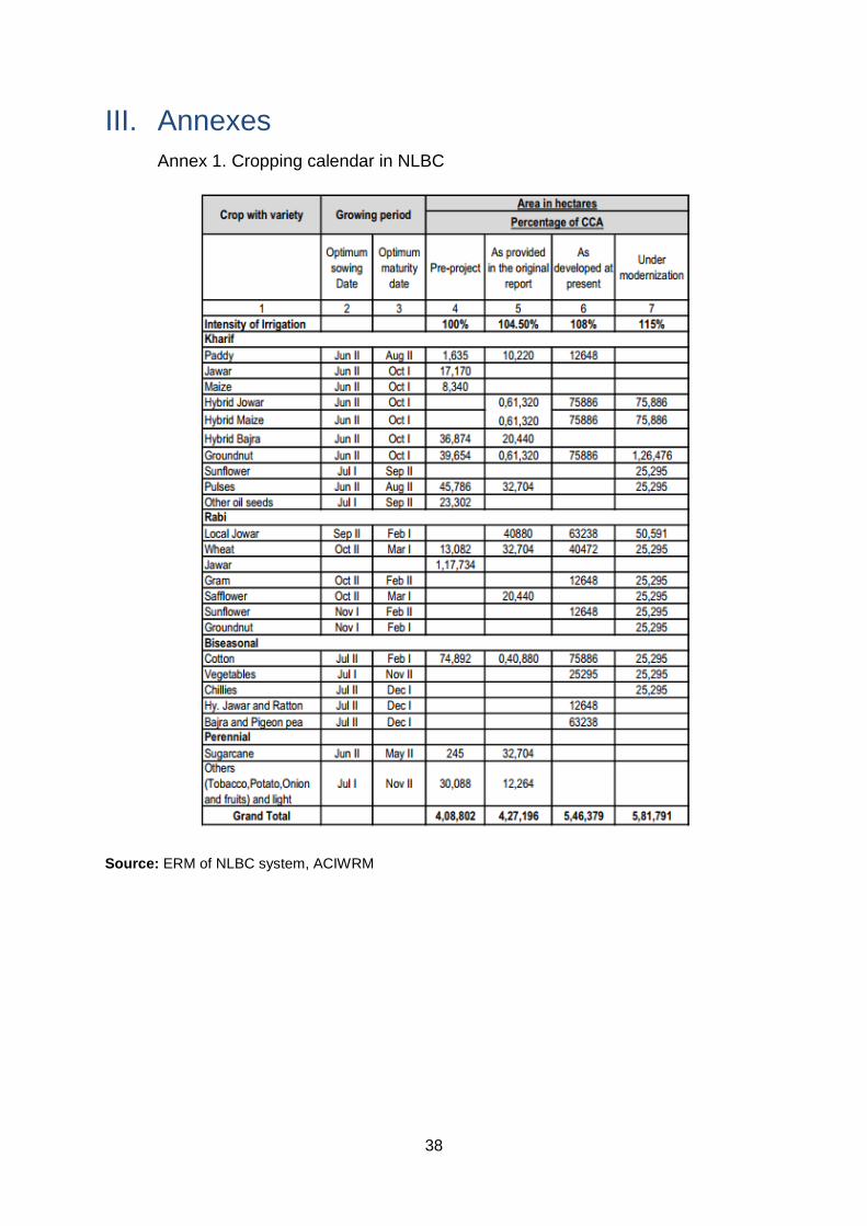
38

III. Annexes

Annex 1. Cropping calendar in NLBC

Source: ERM of NLBC system, ACIWRM

39

Annex 2. Agro-Climatic details of NLBC

Agro Climatic Zones in the command area:

Karnataka has been classified into 10 agroclimatic zones based on (a) Rainfall pattern, quantum

and distribution; (b) Soil types, texture, depth and physico-chemical properties; (c) Elevation and

topography and (d) Major crops. The agro-climatic zones of NLBC is shown in Figure 2-1. The

major five taluks having command area of more than 40% falls in the North Eastern dry Zone and

Northern Dry Zone. In North Eastern Dry Zone the annual rainfall varies from 600 mm to 800

mm/year. About 55 % of the rainfall is received during Rabi season. The elevation ranges from

300-450 m in all taluks. The soils are deep to very deep black clay in major areas and shallow to

medium black in minor pockets. The principal crops grown are Rabi jowar, Bajra, Pulses, Oilseeds

and Cotton.

The annual rainfall in Northern Dry zone ranges from 450 to 750 mm/year and about 52 % of the

annual rainfall is received during Rabi season. The elevation is between 450 to 900 m. The soils

are shallow to deep black clay in major areas. The important crops grown here are Rabi jowar,

Maize, Bajra, Groundnut, Cotton, Wheat, Sugarcane and Tobacco.

Figure 2-1: Agro-climatic zones of NLBC (Source: KSRSAC)

Rainfall in the command area:

The 30 years average annual rainfall (1988 to 2019) in the Narayanpur Left Bank canal command

area varies from 325 to 750 mm/year. Large area of command area has rainfall within 600

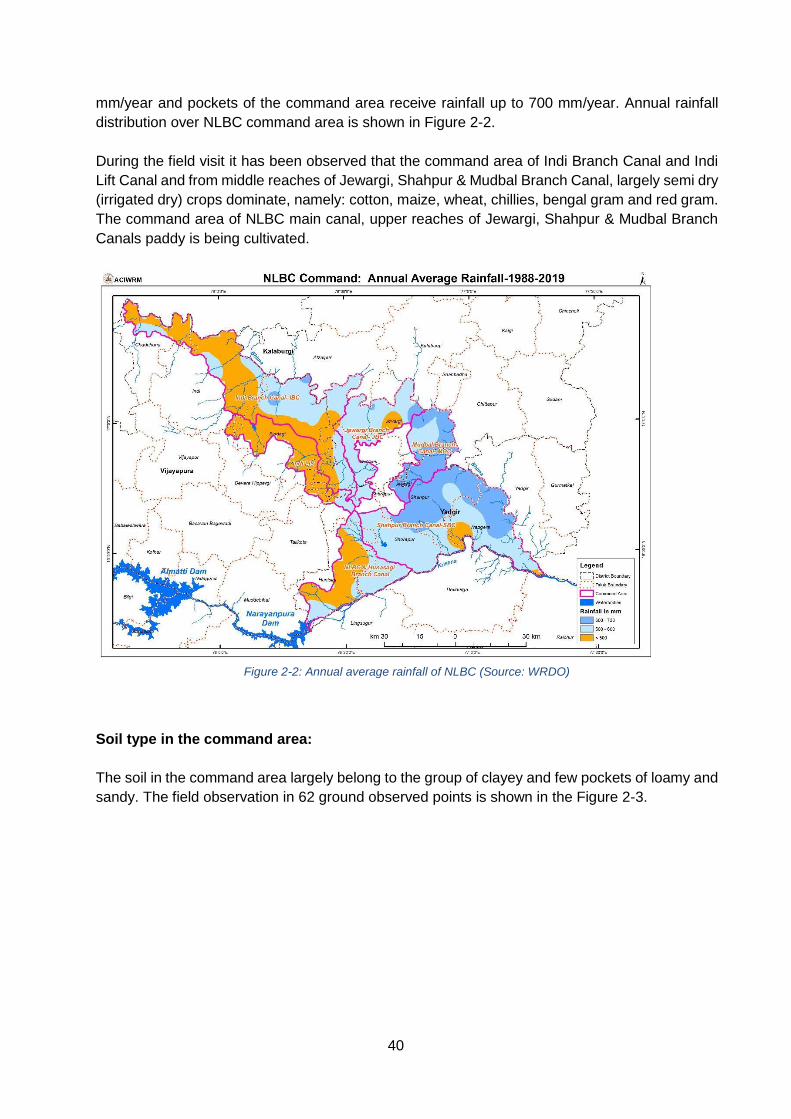
40

mm/year and pockets of the command area receive rainfall up to 700 mm/year. Annual rainfall

distribution over NLBC command area is shown in Figure 2-2.

During the field visit it has been observed that the command area of Indi Branch Canal and Indi

Lift Canal and from middle reaches of Jewargi, Shahpur & Mudbal Branch Canal, largely semi dry

(irrigated dry) crops dominate, namely: cotton, maize, wheat, chillies, bengal gram and red gram.

The command area of NLBC main canal, upper reaches of Jewargi, Shahpur & Mudbal Branch

Canals paddy is being cultivated.

Figure 2-2: Annual average rainfall of NLBC (Source: WRDO)

Soil type in the command area:

The soil in the command area largely belong to the group of clayey and few pockets of loamy and

sandy. The field observation in 62 ground observed points is shown in the Figure 2-3.

41

Figure 2-3: Soil type distribution of NLBC command area

The data published by National Bureau of Soil Survey and Land Use Planning (NBSSLUP)

classifies the soil in command area into textures viz., clayey, loamy and sandy (Figure 2-4). There

is good agreement between the observed data and published data.

Figure 2-4: Soil texture type map of NLBC as per NBSSLUP

Soil depth in command area:

The majority of the farmers during the field visit reported that the soil depth in their fields is more

than 60cm as per the observed points. Distribution chart showing the observed soil depths are

given in Figure 2-5.

71%

10%

16%

1% 2%

NLBC COMMAND AREA SOIL TYPE -OBSERVED

Black

Red gravelly loam

Red loam

Red Clay

Lateritic gravelly

42

Figure 2-5: Graph showing distribution of soil depth in NLBC

The data published by National Bureau of Soil Survey and Land Use Planning (NBSSLUP)

classifies the soil depth in command area as given below in Figure 2-6. The majority area in the

command has soil depth greater than 100 mm. There is good agreement between the observed

data and published data.

Figure 2-6: Map showing distribution of soil depth in NLBC (source: NBSSLUP)

General field observations:

● Excess rain during the present year led to more moisture in soil.

● Crop flowering stage caught with onset of cold led to flower drop in crops.

● Many farmers cultivating red gram used their own seed for sowing.

8%

11%

45%

36%

NLBC COMMAND AREA SOIL DEPTH -OBSERVED

Less than 15 cm

15 - 30 cm

30 - 60 cm

Greater than 60 cm

43

● Only 1-2 irrigations given for cotton this year from canal since area received well spread

rains.

● Paddy followed by paddy practiced in the upper reaches of the canal.

Table 2-1: Details of crops sown and growing period as observed from field

Crop Kharif Rabi Summer

Paddy Transplanted in end of July to first week of Aug. & Harvested in Dec. 15. Long duration (150 days) Most planted variety: BPT Sona

NA First week Dec. seeds sown in nursery, transplanted during end Dec. – second week Jan. & harvest by end Mar.- second week of Apr. Kaveri Sona, Short duration (120 days). Most planted variety: Kaveri Sona

Cotton July- Jan

Red gram July- Jan

Chilly July- Jan

Wheat Oct- Jan

Bajra July- Oct Jan- Apr.

Groundnut Jul- Oct. Dec.- Apr.

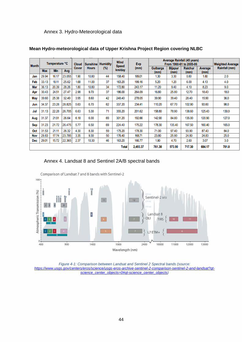
44

Annex 3. Hydro-Meteorological data

Mean Hydro-meteorological data of Upper Krishna Project Region covering NLBC

Annex 4. Landsat 8 and Sentinel 2A/B spectral bands

Figure 4-1: Comparison between Landsat and Sentinel 2 Spectral bands (source:

https://www.usgs.gov/centers/eros/science/usgs-eros-archive-sentinel-2-comparison-sentinel-2-and-landsat?qt-science_center_objects=0#qt-science_center_objects)

https://www.usgs.gov/centers/eros/science/usgs-eros-archive-sentinel-2-comparison-sentinel-2-and-landsat?qt-science_center_objects=0#qt-science_center_objects

https://www.usgs.gov/centers/eros/science/usgs-eros-archive-sentinel-2-comparison-sentinel-2-and-landsat?qt-science_center_objects=0#qt-science_center_objects

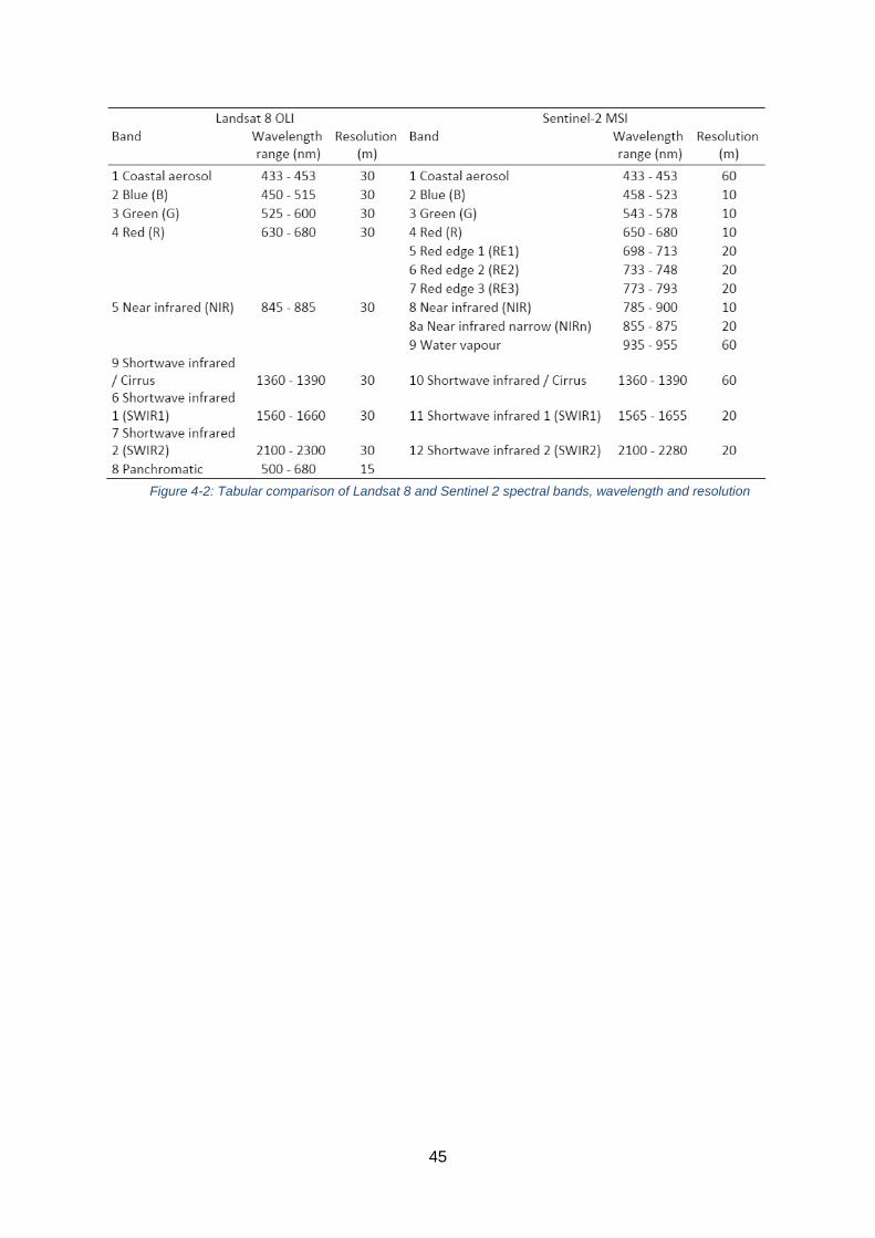
45

Figure 4-2: Tabular comparison of Landsat 8 and Sentinel 2 spectral bands, wavelength and resolution

Additional analyses based on Water Productivity Assessment – NLBC, Karnataka, India

FINAL REPORT

Project final report submitted to the Asian Development Bank under the program for Expanding

Support to Water Accounting in River Basins and Water Productivity in Irrigation Schemes.

Citation: Pareeth, S., Karimi, P. 2020. Additional analyses based on Water Productivity Assessment –

NLBC, Karnataka, India. Project report, IHE Delft Institute for Water Education, The Netherlands.

Cover Image: Farmers in Karnataka. ACIWRM

i

EXPANDING SUPPORT TO WATER ACCOUNTING IN RIVER BASINS AND WATER PRODUCTIVITY IN IRRIGATION SCHEMES

Project final report:

Additional analyses based on Water Productivity Assessment, NLBC,

Karnataka, India

PREPARED FOR THE ASIAN DEVELOPMENT BANK

BY

IHE Delft Institute for Water Education

November 2020

ii

Table of Contents

Table of Contents ii

List of abbreviations iii

List of figures iv

List of tables v

I. Introduction 1

A. Part I: WP activities in Karnataka 1

B. Part II: Additional analyses on water productivity assessment 3

II. Additional analyses on Water Productivity assessment 4

A. Study Area description 4

B. Summary of the approach 5

1. Analysis 1 – Irrigation and rainfall patterns 5

2. Analysis 2 – Irrigation performance in distributary canal command area 5

3. Analysis 3 – Water deficit in DCA’s against proximity to branch canal 8

C. Results 9

1. Analysis 1 – Irrigation and rainfall patterns 9

2. Analysis 2 – Irrigation performance in distributary canal service area 14

3. Analysis 3 - Water deficit in DCA’s against proximity to branch canal 17

D. Key findings 19

III. Annexes 21

Annex 1. Long term rainfall over 20 years from 1999 to 2019 21

Annex 2. Uniformity, RWD, Yield per DCA in NLBC 21

Annex 3. Mean yield per crop and CCA 24

iii

List of abbreviations

ACIWRM Advanced Centre for Integrated Water Resources Management

ADB Asian Development Bank

AGBP Above Ground Biomass Production

AWiFS Advanced Wide Field Sensor

CCA Cultural Command Area

CV Coefficient of Variation

DCA Distributary canal Command Area

ETa Actual Evapotranspiration

FAO Food and Agriculture Organization

FIC Field Irrigation Canal

IHE Delft IHE Delft Institute for Water Education

IRS Indian Remote Sensing

IWMI International Water Management Institute

NRSC National Remote Sensing Centre

NASA National Aeronautics and Space Administration

NLBC Narayanpur Left Bank Canal

ODK Open Data Kit

PySEBAL Python implementation of SEBAL

RWD Relative Water Deficit

SD Standard Deviation

SEBAL Surface Energy Balance Model

SOC Soil Organic Carbon

SRTM Shuttle Radar Topography Mission

TA Technical Assistance

TLBC Tungabhadra Left Bank Canal

TOA Top of Atmosphere

TRMM Tropical Rainfall Measuring Mission

WP Water Productivity

WPy Yield Water Productivity

iv

List of figures

Figure 1: Conceptual framework of training proposed in the project with listed learning

objectives .............................................................................................................................. 3

Figure 2: Study area map; Left – red box in the inset map shows the location of NLBC

command area in the state of Karnataka; Right – NLBC command boundaries with major rivers

............................................................................................................................................. 4

Figure 3: Cropping seasons in NLBC .................................................................................... 5

Figure 4: Schematic view of the NLBC canal network and CCA’s ......................................... 6

Figure 5: Main, branch distributary and tertiary canals in NLBC scheme ............................... 7

Figure 6: Convex hull polygon over a point layer (created using v.hull module in GRASS GIS)

............................................................................................................................................. 7

Figure 7: Delineated DCA boundary of D11 canal in CCA 1 .................................................. 8

Figure 8: Annual irrigated and fallow area in ha derived from NRSC land use maps ............. 9

Figure 9: Monthly rainfall derived from TRMM dataset over CCA’s in NLBC from January 2014

to December 2019. The dry spells are marked in red. ......................................................... 10

Figure 10: Annual land use maps at 60m resolution for five years obtained from NRSC, India.

The variation in different seasonal agriculture is evident from the maps especially the fallow

area over different CCA’s .................................................................................................... 11

Figure 11: Variation in fallow area computed from NRSC maps and the reported seasonal

rainfall over each year from 2014-15 to 2018-19 ................................................................. 12

Figure 12: Land use map of 2018-19 obtained from NRSC and the ETa map of kharif season

2018-1. Red circles highlight large area of fallow land......................................................... 12

Figure 13: Three locations of persistent fallow area over five years from 2014-15 to 2018-19

........................................................................................................................................... 13

Figure 14: Three locations of highest reported persistent fallow area in 2015-16 & 2018-19 14

Figure 15: Left – Scatterplot between cotton yield and uniformity per DCA, right – matrix

showing spearman’s correlation coefficient between crop specific variables and water use,

water deficit parameters ...................................................................................................... 16

Figure 16: Left – Scatterplot between paddy yield and uniformity per DCA, right – matrix



Figure 17: Left – Scatterplot between redgram yield and uniformity per DCA, right – matrix



Figure 18: Left – Scatterplot between ETa and average distance per DCA, right – Scatterplot

between RWD and average distance per DCA.................................................................... 18





v

List of tables

Table 1: CCA supported by branch canals in NLBC .............................................................. 4

Table 2: Rainfall in mm/season during kharif season for five years from 2014-15 to 2018-19.

Dry years are highlighted in red ............................................................................................ 9

Table 3: Persistent fallow area in dry years (2014-15 & 2018-19) over different CCA’s ....... 11

Table 4: Highest reported fallow area in dry years (2014-15 & 2018-19) over different CCA’s

and DCA’s with the reported Uniformity............................................................................... 14

Table 5: List of DCA’s which reported good spatial distribution of water use. Uniformity is

average of three kharif seasons .......................................................................................... 15

1

I. Introduction

1. The Asian Development Bank (ADB) is committed under its Water Operational Plan

2011-2020 to undertake expanded and enhanced analytical work to enable its developing

member countries to secure a deeper and sharper understanding of water issues and

solutions. IHE Delft, in collaboration with the International Water Management Institute (IWMI)

and the Food and Agricultural Organization of the United Nations (FAO), supports ADB in

achieving this objective.

2. The activities proposed for the current Technical Assistance (TA) build on the work

previously undertaken by IHE Delft in cooperation with the ADB to assess crop water

productivity and to assess water resource status in selected basins/countries in Asia. Toward

this, IHE Delft in coordination with local partners is deploying remote sensing-based Water

Productivity (WP) assessment to quantify the crop yield harvested per unit of consumed net

water. Remote sensing (RS) based assessment of WP is based on actual evapotranspiration

(ETa) to estimate net water consumption. We use the in-house developed PySEBAL model to

compute ETa and Above Ground Biomass Production (AGBP) at 30 m spatial resolution over

multiple cropping seasons.

3. This project aimed to contribute to sustainable development in Asia’s irrigation sector,

and to create more value from scarce water resources. India is one of the 5 countries where

advanced technologies to measure WP from satellite data were introduced. The current

project funded by ADB aims to study water productivity and perform water accounting in the

Krishna basin. The Krishna basin is an interstate river system that flows through Maharashtra

(26% of the area), Karnataka (44%), and Andhra Pradesh (30%). The majority of the Krishna

basin about 76% is covered by agricultural area. Irrigated areas have expanded rapidly in the

past 50 years causing a significant decrease in discharge to the sea. The Krishna basin is

facing growing challenges in satisfying the growing water demands and conflicts are arising

because of competing demands. The overall aim of the water productivity study in Karnataka

is to do a water productivity assessment by expanding the methodology used in Phase-I for

Tungabhadra Left Bank Command (TLBC) to a new area and provide detailed analysis. The

work is been carried out in coordination with the Advanced Centre for Integrated Water

Resources Management (ACIWRM).

4. The analyses were presented to ACIWRM in August 2020 during the final workshop

and are presented in the final report. During the meeting a request was made by ACIWRM to

do additional analyses. This report presents these analyses.

A. Part I: WP activities in Karnataka

5. The WP activities in Karnataka were decided during the inception workshop conducted

from July 29 – August 2, 2019 in Belgaum, Karnataka hosted by Visvesvaraya Technological

University. Three major activities with several milestones and deliverables were fixed. The

activities with deliverables are:

- Remote sensing-based WP assessment

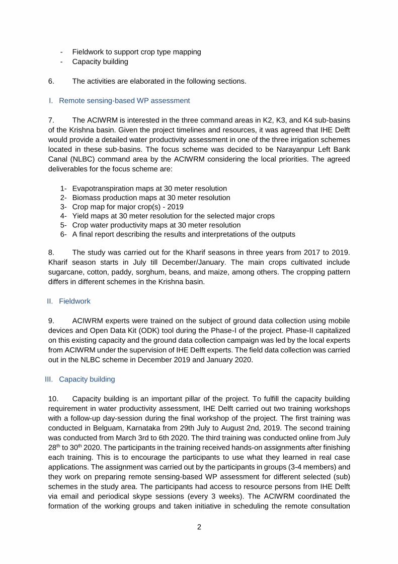
2

- Fieldwork to support crop type mapping

- Capacity building

6. The activities are elaborated in the following sections.

I. Remote sensing-based WP assessment

7. The ACIWRM is interested in the three command areas in K2, K3, and K4 sub-basins

of the Krishna basin. Given the project timelines and resources, it was agreed that IHE Delft

would provide a detailed water productivity assessment in one of the three irrigation schemes

located in these sub-basins. The focus scheme was decided to be Narayanpur Left Bank

Canal (NLBC) command area by the ACIWRM considering the local priorities. The agreed

deliverables for the focus scheme are:

1- Evapotranspiration maps at 30 meter resolution

2- Biomass production maps at 30 meter resolution

3- Crop map for major crop(s) - 2019

4- Yield maps at 30 meter resolution for the selected major crops

5- Crop water productivity maps at 30 meter resolution

6- A final report describing the results and interpretations of the outputs

8. The study was carried out for the Kharif seasons in three years from 2017 to 2019.

Kharif season starts in July till December/January. The main crops cultivated include

sugarcane, cotton, paddy, sorghum, beans, and maize, among others. The cropping pattern

differs in different schemes in the Krishna basin.

II. Fieldwork

9. ACIWRM experts were trained on the subject of ground data collection using mobile

devices and Open Data Kit (ODK) tool during the Phase-I of the project. Phase-II capitalized

on this existing capacity and the ground data collection campaign was led by the local experts

from ACIWRM under the supervision of IHE Delft experts. The field data collection was carried

out in the NLBC scheme in December 2019 and January 2020.

III. Capacity building

10. Capacity building is an important pillar of the project. To fulfill the capacity building

requirement in water productivity assessment, IHE Delft carried out two training workshops

with a follow-up day-session during the final workshop of the project. The first training was

conducted in Belguam, Karnataka from 29th July to August 2nd, 2019. The second training

was conducted from March 3rd to 6th 2020. The third training was conducted online from July

28th to 30th 2020. The participants in the training received hands-on assignments after finishing

each training. This is to encourage the participants to use what they learned in real case

applications. The assignment was carried out by the participants in groups (3-4 members) and

they work on preparing remote sensing-based WP assessment for different selected (sub)

schemes in the study area. The participants had access to resource persons from IHE Delft

via email and periodical skype sessions (every 3 weeks). The ACIWRM coordinated the

formation of the working groups and taken initiative in scheduling the remote consultation

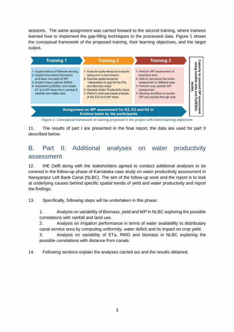
3

sessions. The same assignment was carried forward to the second training, where trainees

learned how to implement the gap-filling techniques to the processed data. Figure 1 shows

the conceptual framework of the proposed training, their learning objectives, and the target

output.

Figure 1: Conceptual framework of training proposed in the project with listed learning objectives

11. The results of part I are presented in the final report, the data are used for part II

described below.

B. Part II: Additional analyses on water productivity

assessment

12. IHE Delft along with the stakeholders agreed to conduct additional analyses to be

covered in the follow-up phase of Karnataka case study on water productivity assessment in

Narayanpur Left Bank Canal (NLBC). The aim of the follow-up work and the report is to look

at underlying causes behind specific spatial trends of yield and water productivity and report

the findings.

13. Specifically, following steps will be undertaken in this phase:

1. Analysis on variability of Biomass, yield and WP in NLBC exploring the possible

correlations with rainfall and land use.

2. Analysis on irrigation performance in terms of water availability to distributary

canal service area by computing uniformity, water deficit and its impact on crop yield.

3. Analysis on variability of ETa, RWD and biomass in NLBC exploring the

possible correlations with distance from canals.

14. Following sections explain the analyses carried out and the results obtained.

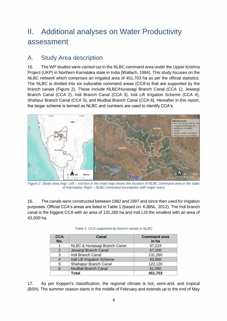
4

II. Additional analyses on Water Productivity

assessment

A. Study Area description

15. The WP studies were carried out in the NLBC command area under the Upper Krishna

Project (UKP) in Northern Karnataka state in India (Wallach, 1984). This study focuses on the

NLBC network which comprises an irrigated area of 451,703 ha as per the official statistics.

The NLBC is divided into six culturable command areas (CCA’s) that are supported by the

branch canals (Figure 2). These include NLBC/Hunasagi Branch Canal (CCA 1), Jewargi

Branch Canal (CCA 2), Indi Branch Canal (CCA 3), Indi Lift Irrigation Scheme (CCA 4),

Shahpur Branch Canal (CCA 5), and Mudbal Branch Canal (CCA 6). Hereafter in this report,

the larger scheme is termed as NLBC and numbers are used to identify CCA’s.

Figure 2: Study area map; Left – red box in the inset map shows the location of NLBC command area in the state

of Karnataka; Right – NLBC command boundaries with major rivers

16. The canals were constructed between 1982 and 1997 and since then used for irrigation

purposes. Official CCA’s areas are listed in Table 1 (based on: KJBNL, 2012). The Indi branch

canal is the biggest CCA with an area of 131,260 ha and Indi LIS the smallest with an area of

43,000 ha.

Table 1: CCA supported by branch canals in NLBC

CCA No.

Canal Command area in ha

1 NLBC & Hunasagi Branch Canal 47,223

2 Jewargi Branch Canal 57,100

3 Indi Branch Canal 131,260

4 Indi Lift Irrigation Scheme 43,000

5 Shahapur Branch Canal 122,120

6 Mudbal Branch Canal 51,000

Total 451,703

17. As per Koppen's classification, the regional climate is hot, semi-arid, and tropical

(BSh). The summer season starts in the middle of February and extends up to the end of May

5

or the beginning of June. The summer is followed by the southwest monsoon season from

June up to the end of September. The northeast or the retreating monsoon season is the

period from October to November, while the winter season is from December to the middle of

February. There are two main cropping seasons of Kharif and Rabi. The beginning and length

of the cropping seasons in this region could vary from one year to another depending on the

rainfall and the timing of monsoons. In general, however, Kharif season starts in July and ends

in December or early January. Rabi season follows Kharif and will continue until the end of

March and could extend to April. There is a third cropping season, Zaid, which is a short

season lasting on average for 2 months and starting in April. In the NLBC, however, the

cultivated area in the Zaid season is very small and almost negligible.

Figure 3: Cropping seasons in NLBC

The project region has an average annual rainfall of 700 mm/year. During Kharif season the

average rainfall is 520 mm/season. The seasonal ETa over CCA’s in NLBC vary from 300 to

600 mm/season. The climatic variability over time is high with frequent dry years. December

is the coldest month of the year with an average temperature of 22.4 °C and May is the hottest

with an average temperature of 32.5 °C. With the onset of monsoon, the weather becomes

cooler. The months from December to May are the driest.

B. Summary of the approach

1. Analysis 1 – Irrigation and rainfall patterns

18. Irrigation in NLBC takes place mainly during two seasons – Rabi and Kharif (Figure 3).

The extent of irrigated land within different CCA’s in NLBC, identified using satellite data,

shows high spatial and temporal variability. In this analysis, annual land use maps from 2014-

15 to 2018-19 obtained from National Remote Sensing Centre (NRSC) with high spatial

resolution (60 m) were used to understand the land use variations. In addition, monthly and

annual rainfall data obtained from Tropical Rainfall Measuring Mission (TRMM) data was used

to determine the dry and wet seasons and its effect on irrigated land use. Further, a canal

network layer is used to conduct proximity analysis to understand the most affected areas with

respect to supplied water availability in dry seasons.

2. Analysis 2 – Irrigation performance in distributary canal command

area

19. NLBC is the main irrigation canal from the Narayanpur dam which is augmented by

the storage created in the Almatti dam. The main canal provides water for the canal branches

that run through the network and carry water to different CCA’s. Figure 4 illustrates the

schematic view of the distribution network and the location on the CCA’s in relation to the

6

branch canals. The CCA 1 is close to the water source (i.e. Narayanpur Dam), and areas in

the northwest end of the CCA 3 are furthest. Bhima river defines the border of the NLBC to

the north and west and the Krishna river delimits the southern border. These rivers also act

as final drainage outfall for the network and as a source of water for farmers who are close to

the rivers. The farmers downstream tend to extract water directly from these rivers when the

water supply from the network is interrupted or is deemed insufficient.

Figure 4: Schematic view of the NLBC canal network and CCA’s

20. The water from branch canals are further distributed through distributary canals

(secondary) which feed water to the lateral, sub-lateral and then to field irrigation channels

(FIC). ACIWRM obtained data of the canal network covering main, branch and distributary

canals in CCA’s – 1, 2, 3, 5 and 6. There are around 200 distributary canal networks in these

CCA’s which distribute water for irrigation. Figure 5 shows the main, branch and distributary

canal network in the CCA’s. Note that the canal network for CCA 4 is not available, hence

avoided from the further analysis.

7

Figure 5: Main, branch distributary and tertiary canals in NLBC scheme

21. To analyze the water distribution in terms of water use, deficit, yield and WP for each

Distributary canal Command Area (DCA) it is important to delineate the boundary of each

distribution canal network. Though such a boundary often does not exist or difficult to obtain.

An approach using delineating minimum bounds from a vector layer was used to extract the

possible distributary canal service area. In principle a convex hull was drawn connecting the

nodes of linear two-dimensional network representing a distributary canal network

encompassing the minimum possible bounding box. The convex hull, or convex envelope, for

an object or a set of objects is the minimal convex set containing the given objects. Figure 6

represents the convex hull principle on a vector point layer.

Figure 6: Convex hull polygon over a point layer (created using v.hull module in GRASS GIS)

22. Similarly, convex hull polygon encapsulating the minimum bounding box of each

distributary canal was developed. Further a buffer of 150 m was added to the delineated

boundary to include possible reach of respective canals. These spatial analysis steps were

executed for 200 distributary canal networks. Out of these 200 delineated DCA’s, 127 were

selected with areas varying from 275 to 16,300 ha for further analysis. The analyses focused

on the performance within the canal network and also in perspective of the location of the

8

network in entire NLBC. Figure 7 shows one such delineated boundary of distributary canal

D11 in CCA 1.

Figure 7: Delineated DCA boundary of D11 canal in CCA 1

23. One of the limitations of this approach to delineate DCA’s is that there could be overlap

at the edges with neighboring DCA’s. The DCA’s with uncertain boundaries were removed

from further analysis to avoid discrepancy in the aggregated statistics. Though, the analysis

when carried out using spatially aggregated statistics such as average or median reduced the

uncertainties due to errors in boundary delineation.

24. Aggregated statistics from various outputs of the WP assessment were extracted for

127 delineated DCA’s for further analysis. Additionally, an irrigation performance indicator

called uniformity was computed for each DCA. The uniform distribution of water resources is

related to the spatial distribution of water consumption. Uniformity represents the spatial

distribution of water use among the DCA’s. The performance indicator uniformity was

calculated per DCA by computing coefficient of variation (CV) of water use (seasonal ETa).

Following equation was used to compute uniformity.

25. Where numerator is mean of ETa per DCA and SD is standard deviation of ETa.

3. Analysis 3 – Water deficit in DCA’s against proximity to branch canal

26. Once the DCA boundaries are delineated, a detailed analysis was carried out by

extracting the aggregated statistics of layers related to water productivity assessment. The

average ETa, RWD, biomass, crop yield, Crop Water Productivity (WPy) and distance of each

distributary canal network from the source branch canal was extracted and analyzed.

27. To understand the drivers behind varying performance in terms of yield and water

productivity, the extracted statistics of water productivity assessment layers were compared

with average distance to branch canal of respective CCA. Correlation coefficient was

computed between water productivity layers and the distance to assess the impact.

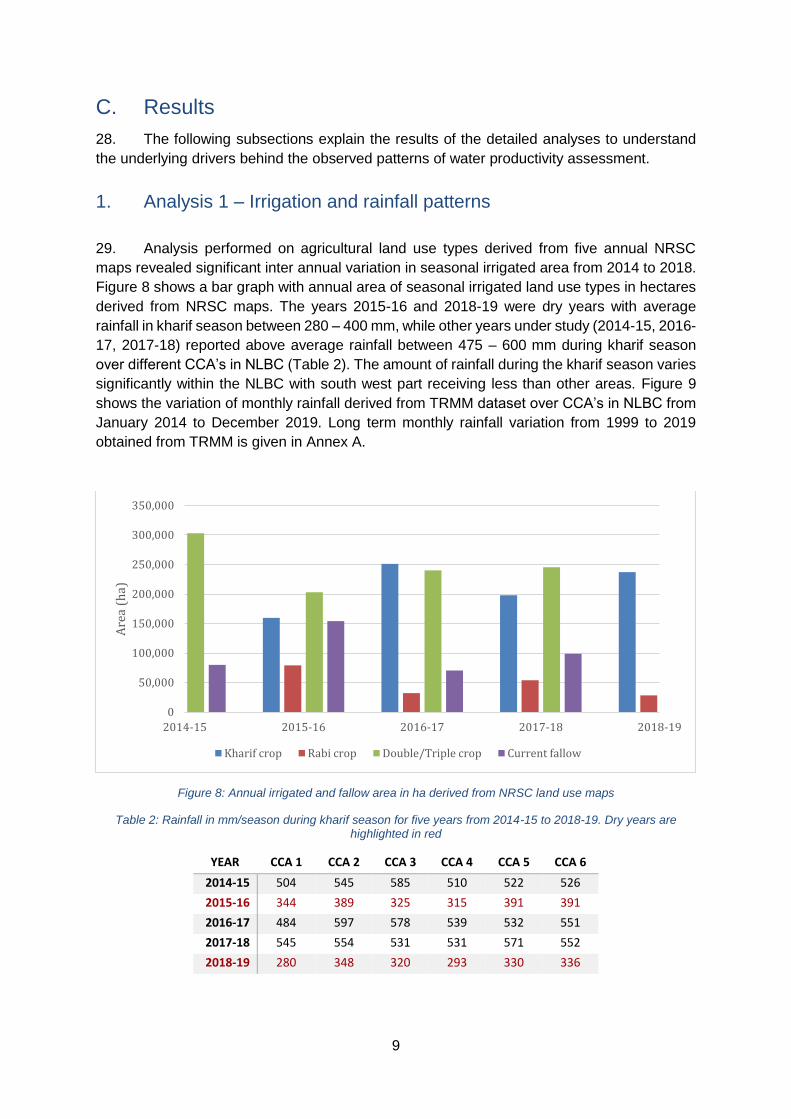
9

C. Results

28. The following subsections explain the results of the detailed analyses to understand

the underlying drivers behind the observed patterns of water productivity assessment.

1. Analysis 1 – Irrigation and rainfall patterns

29. Analysis performed on agricultural land use types derived from five annual NRSC

maps revealed significant inter annual variation in seasonal irrigated area from 2014 to 2018.

Figure 8 shows a bar graph with annual area of seasonal irrigated land use types in hectares

derived from NRSC maps. The years 2015-16 and 2018-19 were dry years with average

rainfall in kharif season between 280 – 400 mm, while other years under study (2014-15, 2016-

17, 2017-18) reported above average rainfall between 475 – 600 mm during kharif season

over different CCA’s in NLBC (Table 2). The amount of rainfall during the kharif season varies

significantly within the NLBC with south west part receiving less than other areas. Figure 9

shows the variation of monthly rainfall derived from TRMM dataset over CCA’s in NLBC from

January 2014 to December 2019. Long term monthly rainfall variation from 1999 to 2019

obtained from TRMM is given in Annex A.

Figure 8: Annual irrigated and fallow area in ha derived from NRSC land use maps

Table 2: Rainfall in mm/season during kharif season for five years from 2014-15 to 2018-19. Dry years are highlighted in red

YEAR CCA 1 CCA 2 CCA 3 CCA 4 CCA 5 CCA 6

2014-15 504 545 585 510 522 526

2015-16 344 389 325 315 391 391

2016-17 484 597 578 539 532 551

2017-18 545 554 531 531 571 552

2018-19 280 348 320 293 330 336

0

50,000

100,000

150,000

200,000

250,000

300,000

350,000

2014-15 2015-16 2016-17 2017-18 2018-19

Are

a (h

a)

Kharif crop Rabi crop Double/Triple crop Current fallow

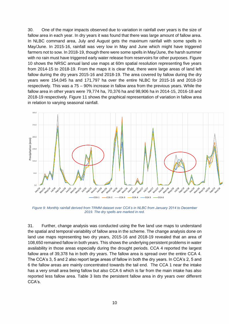
10

30. One of the major impacts observed due to variation in rainfall over years is the size of

fallow area in each year. In dry years it was found that there was large amount of fallow area.

In NLBC command area, July and August gets the maximum rainfall with some spells in

May/June. In 2015-16, rainfall was very low in May and June which might have triggered

farmers not to sow. In 2018-19, though there were some spells in May/June, the harsh summer

with no rain must have triggered early water release from reservoirs for other purposes. Figure

10 shows the NRSC annual land use maps at 60m spatial resolution representing five years

from 2014-15 to 2018-19. From the maps it is clear that, there were large areas of land left

fallow during the dry years 2015-16 and 2018-19. The area covered by fallow during the dry

years were 154,045 ha and 171,797 ha over the entire NLBC for 2015-16 and 2018-19

respectively. This was a 75 – 90% increase in fallow area from the previous years. While the

fallow area in other years were 79,774 ha, 70,376 ha and 98,906 ha in 2014-15, 2016-18 and

2018-19 respectively. Figure 11 shows the graphical representation of variation in fallow area

in relation to varying seasonal rainfall.

Figure 9: Monthly rainfall derived from TRMM dataset over CCA’s in NLBC from January 2014 to December 2019. The dry spells are marked in red.

31. Further, change analysis was conducted using the five land use maps to understand

the spatial and temporal variability of fallow area in the scheme. The change analysis done on

land use maps representing two dry years, 2015-16 and 2018-19 revealed that an area of

108,650 remained fallow in both years. This shows the underlying persistent problems in water

availability in those areas especially during the drought periods. CCA 4 reported the largest

fallow area of 39,378 ha in both dry years. The fallow area is spread over the entire CCA 4.

The CCA’s 3, 5 and 2 also report large areas of fallow in both the dry years. In CCA’s 2, 5 and

6 the fallow areas are mainly concentrated towards the tail end. The CCA 1 near the intake

has a very small area being fallow but also CCA 6 which is far from the main intake has also

reported less fallow area. Table 3 lists the persistent fallow area in dry years over different

CCA’s.

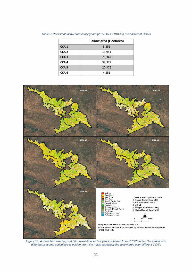
11

Table 3: Persistent fallow area in dry years (2014-15 & 2018-19) over different CCA’s

Fallow area (Hectares)

CCA 1 5,356

CCA 2 13,941

CCA 3 25,347

CCA 4 39,377

CCA 5 20,376

CCA 6 4,251

Figure 10: Annual land use maps at 60m resolution for five years obtained from NRSC, India. The variation in

different seasonal agriculture is evident from the maps especially the fallow area over different CCA’s

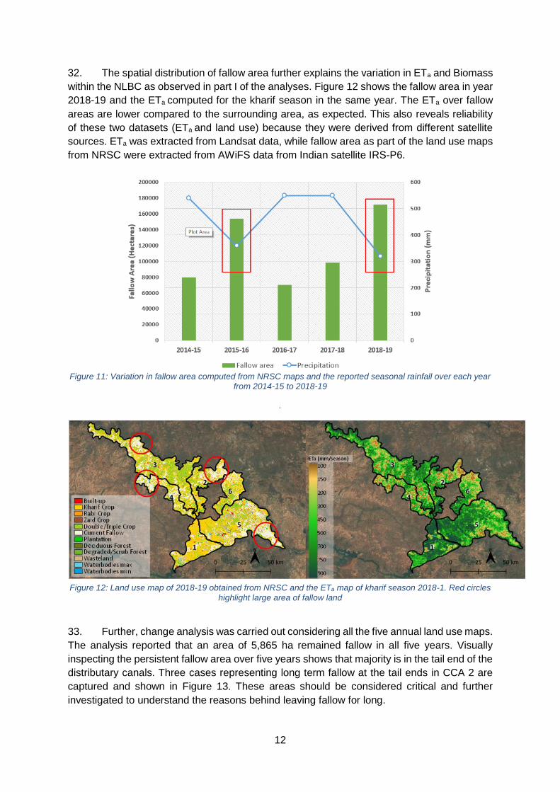
12

32. The spatial distribution of fallow area further explains the variation in ETa and Biomass

within the NLBC as observed in part I of the analyses. Figure 12 shows the fallow area in year

2018-19 and the ETa computed for the kharif season in the same year. The ETa over fallow

areas are lower compared to the surrounding area, as expected. This also reveals reliability

of these two datasets (ETa and land use) because they were derived from different satellite

sources. ETa was extracted from Landsat data, while fallow area as part of the land use maps

from NRSC were extracted from AWiFS data from Indian satellite IRS-P6.

Figure 11: Variation in fallow area computed from NRSC maps and the reported seasonal rainfall over each year

from 2014-15 to 2018-19

.

Figure 12: Land use map of 2018-19 obtained from NRSC and the ETa map of kharif season 2018-1. Red circles

highlight large area of fallow land

33. Further, change analysis was carried out considering all the five annual land use maps.

The analysis reported that an area of 5,865 ha remained fallow in all five years. Visually

inspecting the persistent fallow area over five years shows that majority is in the tail end of the

distributary canals. Three cases representing long term fallow at the tail ends in CCA 2 are

captured and shown in Figure 13. These areas should be considered critical and further

investigated to understand the reasons behind leaving fallow for long.

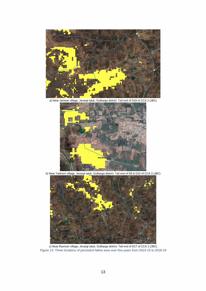
13

a) Near Janiwar village, Jevargi taluk, Gulbarga district. Tail end of D18 of CCA 2 (JBC)

b) Near Yadrami village, Jevargi taluk, Gulbarga district. Tail end of D9 & D10 of CCA 2 (JBC)

c) Near Ravnoor village, Jevargi taluk, Gulbarga district. Tail end of D17 of CCA 2 (JBC)

Figure 13: Three locations of persistent fallow area over five years from 2014-15 to 2018-19

14

2. Analysis 2 – Irrigation performance in distributary canal service area

34. Delineating boundary of 127 DCA’s helped in localizing the analysis to find important

patterns at field level. Table 4 shows the distributary canals with more than 1,000 ha of

persistent fallow land in dry years. The highest reported fallow area of 3,300 ha in both dry

years was in DCA, D18 of CCA 2 (JBC), followed by D6 of CCA 5 (2,600 ha), D24 of CCA 3

(2,400 ha) and D22 of CCA 3 (2,000 ha). CCA’s 2, 3 and 5 had DCAs with fallow area greater

than 2,000 ha. The DCAs with larger fallow areas also reported lower uniformity which shows

weaker water distribution in this area which may have left farmers without water especially

during the dry years. Figure 14 shows three locations of persistent fallow area as examples in

the tail end of DCA’s in CCA 2, 3 & 5.

Table 4: Highest reported fallow area in dry years (2014-15 & 2018-19) over different CCA’s and DCA’s with the

reported Uniformity

CCA DCA Fallow area in ha (2015-16 / 2018-19)

Total area in ha % fallow land Uniformity (%)

CCA 2 D18 of JBC 3,300 8,227 40 77

CCA 5 D6 of SBC 2,600 16,321 16 31

CCA 3 D24 of IBC 2,400 3,388 71 61

CCA 3 D22 of IBC 2,000 5,725 35 44

CCA 2 D14 of JBC 1,870 4,337 43 63

CCA 3 D25 of IBC 1,450 3,787 38 52

CCA 5 D9 of SBC 1,410 7,243 19 54

CCA 3 D20 of IBC 1,200 2,334 51 63

CCA 3 D46 of IBC 1,100 2,203 50 45

CCA 2 BD3 of D12 of JBC 1,100 3,038 36 53

CCA 5 D14 of SBC 1,000 4,191 24 51

CCA 5 D21 of SBC 1,000 3,875 26 33

Figure 14: Three locations of highest reported persistent fallow area in 2015-16 & 2018-19

15

35. The uniformity computed for DCA’s in NLBC varied from 10% to 70%. CCA 1 reported

highest uniformity among DCA’s with an average Coefficient of Variation (CV) of 20% which

means good distribution of water. CCA 5 reported an average uniformity with CV of 30%

among DCA’s which means the water distribution is fair but need improvement. CCA’s 2, 3

and 6 reported an average uniformity with CV of 40% among DCA’s which means the water

distribution is not good. The best performing DCA’s in terms of uniformity are listed in Table

5.

Table 5: List of DCA’s which reported good spatial distribution of water use. Uniformity is average of three kharif

seasons

CCA DCA name Uniformity (%)

CCA 1 Kakkera Major Distributary of D5 11

CCA 1 D12 13

CCA 1 D10 14

CCA 1 D11 14

CCA 1 D9 17

CCA 1 Hunasihole Distributary of Kakkera 18

CCA 1 D2 19

CCA 1 10A 19

CCA 1 3C 20

CCA 2 D6 19

CCA 2 2B 20

CCA 3 12A 15

CCA 5 3A 14

CCA 5 D4 18

CCA 5 SD1/D2 of SBC 20

CCA 6 22B 20

36. A complete list of DCA’s and uniformity is provided in Annex B. Further, to understand

the impact of varying water distribution in the scheme among DCA’s correlation analysis was

carried out between output (production parameters like yield) and input (water availability

related parameters like uniformity and RWD). Figure 15, 16 and 17 shows correlation between

aggregated yield and uniformity per DCA for cotton, paddy and redgram respectively. The

scatterplots (left plot in Figures 15, 16 and 17) shows clear negative correlation between yield

and uniformity. The scatterplots are color coded according to the CCA’s.

37. For cotton, a strong negative correlation coefficient (Spearman’s R) of -0.62 was

reported between yield and uniformity over all the DCA’s in different CCA’s. The negative trend

is not strong in CCA 1 & 5, close to head of the scheme with overall good uniformity. But

negative correlation is strong in CCA 2, 3 and 6 where it is clear that yield produced is

decreased with less uniform water distribution. This trend is further substantiated by the strong

negative correlation between Yield and RWD, which reported a correlation coefficient of -0.8

(Figure 15).

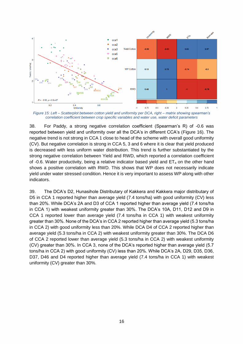
16

Figure 15: Left – Scatterplot between cotton yield and uniformity per DCA, right – matrix showing spearman’s

correlation coefficient between crop specific variables and water use, water deficit parameters

38. For Paddy, a strong negative correlation coefficient (Spearman’s R) of -0.6 was

reported between yield and uniformity over all the DCA’s in different CCA’s (Figure 16). The

negative trend is not strong in CCA 1 close to head of the scheme with overall good uniformity

(CV). But negative correlation is strong in CCA 5, 3 and 6 where it is clear that yield produced

is decreased with less uniform water distribution. This trend is further substantiated by the

strong negative correlation between Yield and RWD, which reported a correlation coefficient

of -0.6. Water productivity, being a relative indicator based yield and ETa on the other hand

shows a positive correlation with RWD. This shows that WP does not necessarily indicate

yield under water stressed condition. Hence it is very important to assess WP along with other

indicators.

39. The DCA’s D2, Hunasihole Distributary of Kakkera and Kakkera major distributary of

D5 in CCA 1 reported higher than average yield (7.4 tons/ha) with good uniformity (CV) less

than 20%. While DCA’s 2A and D3 of CCA 1 reported higher than average yield (7.4 tons/ha

in CCA 1) with weakest uniformity greater than 30%. The DCA’s 10A, D11, D12 and D9 in

CCA 1 reported lower than average yield (7.4 tons/ha in CCA 1) with weakest uniformity

greater than 30%. None of the DCA’s in CCA 2 reported higher than average yield (5.3 tons/ha

in CCA 2) with good uniformity less than 20%. While DCA D4 of CCA 2 reported higher than

average yield (5.3 tons/ha in CCA 2) with weakest uniformity greater than 30%. The DCA D6

of CCA 2 reported lower than average yield (5.3 tons/ha in CCA 2) with weakest uniformity

(CV) greater than 30%. In CCA 3, none of the DCA’s reported higher than average yield (5.7

tons/ha in CCA 2) with good uniformity (CV) less than 20%. While DCA’s 2A, D29, D35, D36,

D37, D46 and D4 reported higher than average yield (7.4 tons/ha in CCA 1) with weakest

uniformity (CV) greater than 30%.

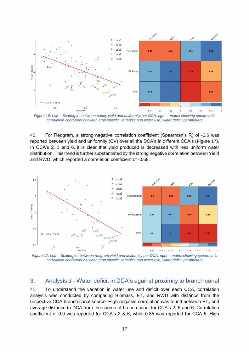
17

Figure 16: Left – Scatterplot between paddy yield and uniformity per DCA, right – matrix showing spearman’s


40. For Redgram, a strong negative correlation coefficient (Spearman’s R) of -0.6 was

reported between yield and uniformity (CV) over all the DCA’s in different CCA’s (Figure 17).

In CCA’s 2, 3 and 6, it is clear that yield produced is decreased with less uniform water

distribution. This trend is further substantiated by the strong negative correlation between Yield

and RWD, which reported a correlation coefficient of -0.68.

Figure 17: Left – Scatterplot between redgram yield and uniformity per DCA, right – matrix showing spearman’s


3. Analysis 3 - Water deficit in DCA’s against proximity to branch canal

41. To understand the variation in water use and deficit over each CCA, correlation

analysis was conducted by comparing Biomass, ETa and RWD with distance from the

respective CCA branch canal source. High negative correlation was found between ETa and

average distance to DCA from the source of branch canal for CCA’s 2, 5 and 6. Correlation

coefficient of 0.9 was reported for CCA’s 2 & 6, while 0.85 was reported for CCA 5. High

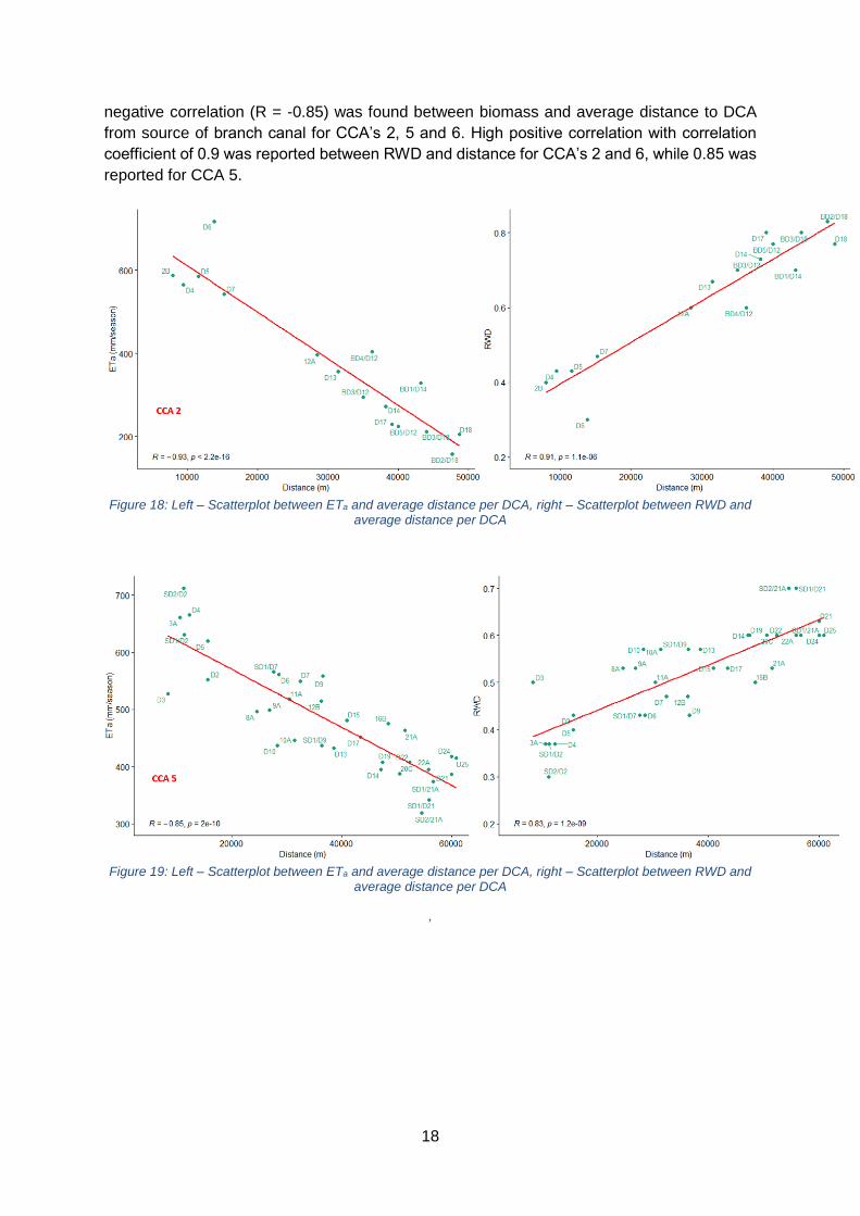
18

negative correlation (R = -0.85) was found between biomass and average distance to DCA

from source of branch canal for CCA’s 2, 5 and 6. High positive correlation with correlation

coefficient of 0.9 was reported between RWD and distance for CCA’s 2 and 6, while 0.85 was

reported for CCA 5.

Figure 18: Left – Scatterplot between ETa and average distance per DCA, right – Scatterplot between RWD and

average distance per DCA



,

19



,

Figure 18, 19 and 20 shows scatterplot between ETa and distance (Left), RWD and distance

(Right) in CCA’s 2, 5 and 6 respectively. The scatterplot clearly shows the linear relation of

ETa and RWD with distance to source of branch canal. As the distance from branch canal

increase, the DCA’s were found to be facing more water deficit issues. The DCA’s in CCA 1

and 3 did not reveal any pattern with respect to distance from branch canals. In CCA 1, this

might be due to high uniformity reported which demonstrate good water distribution.

D. Key findings

42. Analysis performed on agricultural land use types derived from five annual NRSC

maps revealed significant variation in seasonal irrigated area over the years from 2014 to

2018. The area covered by fallow during the dry years were 154,045 ha and 171,797 ha over

the entire NLBC for 2015-16 and 2018-19 respectively. There was a 75 – 90% increase in

fallow area from the previous (wetter) years.

43. The change analysis done on land use maps representing two dry years, 2015-16 and

2018-19 revealed that an area of 108,650 remained fallow in both years, driven by the lack of

rainfall. An area of 5,865 ha remained fallow in all five years. Visually inspecting this persistent

fallow area over five years shows that majority are in the tail end of the distributary canals.

These areas need immediate attention to rejuvenate the crop production.

44. Distributary canal Service Area (DCA) were delineated using spatial analysis tools over

secondary and tertiary canal network provided by ACIWRM. Around 127 DCA’s spanning all

over the five CCA’s in NLBC were selected for further analysis. The highest reported fallow

area of 3,300 ha in both dry years was in DCA, D18 of CCA 2 (JBC), followed by D6 of CCA

5 (2,600 ha), D24 of CCA 3 (2,400 ha) and D22 of CCA 3 (2,000 ha). CCA’s 2, 3 and 5 had

DCA with fallow area greater than 2,000 ha. The DCA’s with larger fallow areas also reported

lower uniformity which shows weaker water distribution in this area which may have left

farmers without water especially during the dry years.

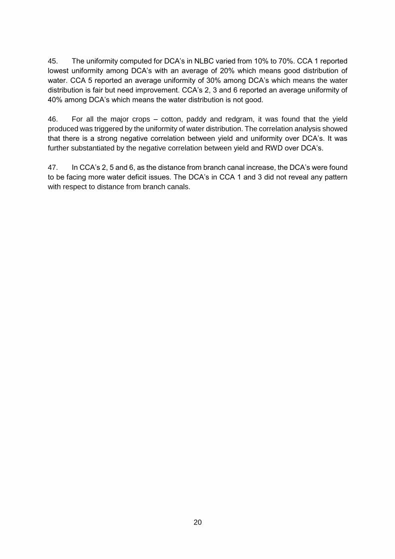
20

45. The uniformity computed for DCA’s in NLBC varied from 10% to 70%. CCA 1 reported

lowest uniformity among DCA’s with an average of 20% which means good distribution of

water. CCA 5 reported an average uniformity of 30% among DCA’s which means the water

distribution is fair but need improvement. CCA’s 2, 3 and 6 reported an average uniformity of

40% among DCA’s which means the water distribution is not good.

46. For all the major crops – cotton, paddy and redgram, it was found that the yield

produced was triggered by the uniformity of water distribution. The correlation analysis showed

that there is a strong negative correlation between yield and uniformity over DCA’s. It was

further substantiated by the negative correlation between yield and RWD over DCA’s.

47. In CCA’s 2, 5 and 6, as the distance from branch canal increase, the DCA’s were found

to be facing more water deficit issues. The DCA’s in CCA 1 and 3 did not reveal any pattern

with respect to distance from branch canals.

21

III. Annexes

Annex 1. Long term rainfall over 20 years from 1999 to 2019

Figure A1: Long term monthly Rainfall derived from TRMM dataset from 1999 to 2019.

Annex 2. Uniformity, RWD, Yield per DCA in NLBC

DCA CCA RWD Uniformity Yield Redgram Yield Paddy Yield Cotton

10A CCA 1 0.30 0.19 6.55 3.15 0.49

2A CCA 1 0.53 0.31 7.57 2.74 0.84

3C CCA 1 0.53 0.20 8.56 3.36 0.64

3D CCA 1 0.37 0.24 8.74 3.61 0.68

5B CCA 1 0.30 0.22 8.15 3.40 0.59

BTSD/D5 CCA 1 0.57 0.48 7.49 2.88 0.57

D1 CCA 1 0.50 0.21 9.03 3.73 0.61

D10 CCA 1 0.30 0.14 7.27 3.97 0.60

D11 CCA 1 0.30 0.14 6.18 3.12 0.48

D12 CCA 1 0.30 0.13 7.17 2.73 0.46

D1 CCA 1 0.53 0.25 8.57 3.51 0.48

D2 CCA 1 0.60 0.27 8.03 3.71 0.89

D2 CCA 1 0.40 0.19 8.94 3.80 0.67

D3 CCA 1 0.33 0.33 9.36 3.92 0.51

D6 CCA 1 0.30 0.21 8.13 2.88 0.47

D6 CCA 1 0.43 0.41 6.73 3.06 0.55

D7 CCA 1 0.37 0.31 7.19 2.52 0.79

D8 CCA 1 0.37 0.21 6.36 3.00 0.47

D9 CCA 1 0.33 0.17 6.41 2.85 0.62

Hanamsagar/3D CCA 1 0.50 0.25 8.55 3.59 0.53

Hosur/D5 CCA 1 0.40 0.25 8.53 3.96 0.52

22

Hunasihole CCA 1 0.50 0.18 7.81 3.91 0.69

Kakkera/D5 CCA 1 0.30 0.11 7.68 4.06 0.61

Manjalapura/D5 CCA 1 0.43 0.21 7.78 3.58 0.61

Rayagera/D5 CCA 1 0.50 0.23 6.90 2.80 0.47

Rayangola/D1 CCA 1 0.60 0.25 9.64 4.07 0.70

12A CCA 2 0.60 0.26 5.61 2.41 0.62

2B CCA 2 0.40 0.20 5.91 2.77 0.42

BD1/D14 CCA 2 0.70 0.48 5.85 1.99 0.58

BD2/D18 CCA 2 0.83 0.70 3.14 1.27 0.72

BD3/D12 CCA 2 0.70 0.45 5.26 2.26 0.54

BD3/D18 CCA 2 0.80 0.53 3.66 1.52 0.71

BD4/D12 CCA 2 0.60 0.25 5.85 2.36 0.63

BD5/D12 CCA 2 0.77 0.66 4.06 1.50 0.56

D13 CCA 2 0.67 0.37 7.72 3.22 0.69

D14 CCA 2 0.73 0.51 4.46 2.16 0.69

D17 CCA 2 0.80 0.50 3.57 1.60 0.70

D18 CCA 2 0.77 0.67 3.37 1.41 0.76

D4 CCA 2 0.43 0.31 6.91 2.48 0.77

D5 CCA 2 0.43 0.39 4.81 1.80 0.67

D6 CCA 2 0.30 0.19 4.40 3.12 0.50

D7 CCA 2 0.47 0.40 4.07 2.56 0.52

12A CCA 3 0.60 0.15 5.11 2.04 0.74

14A CCA 3 0.63 0.26 6.68 2.85 0.60

17A CCA 3 0.63 0.28 4.99 2.15 0.65

19A CCA 3 0.73 0.38 4.17 1.92 0.95

2A CCA 3 0.50 0.36 6.32 2.19 0.67

2B CCA 3 0.73 0.60 4.49 1.71 0.69

5A CCA 3 0.63 0.39 5.47 1.97 0.53

5B CCA 3 0.73 0.55 4.34 1.98 0.68

D10 CCA 3 0.73 0.41 4.08 1.53 0.77

D12 CCA 3 0.63 0.29 5.64 2.14 0.83

D13 CCA 3 0.60 0.33 5.56 2.18 0.67

D14 CCA 3 0.70 0.32 4.93 1.94 0.59

D15 CCA 3 0.67 0.21 5.02 2.01 0.63

D16 CCA 3 0.60 0.30 5.32 2.22 0.58

D19 CCA 3 0.70 0.32 4.11 2.09 0.83

D20 CCA 3 0.77 0.39 4.39 1.87 0.98

D21 CCA 3 0.73 0.35 4.32 1.84 0.87

D22 CCA 3 0.73 0.43 4.34 1.89 0.92

D24 CCA 3 0.77 0.55 4.15 1.90 0.82

D25 CCA 3 0.67 0.48 5.26 2.40 0.72

D26 CCA 3 0.67 0.31 4.73 2.32 0.64

D28 CCA 3 0.67 0.32 4.47 2.15 0.69

D29 CCA 3 0.63 0.31 6.72 2.92 0.67

23

D35 CCA 3 0.60 0.34 6.15 2.70 0.70

D36 CCA 3 0.57 0.37 7.55 2.71 0.70

D37 CCA 3 0.57 0.30 6.50 2.60 0.69

D44 CCA 3 0.43 0.30 9.89 3.57 0.43

D46 CCA 3 0.60 0.43 7.91 2.62 0.55

D4 CCA 3 0.50 0.33 6.03 2.12 0.66

D7 CCA 3 0.80 0.42 2.98 1.27 0.47

D9 CCA 3 0.73 0.43 3.71 1.52 0.69

SD1/D13 CCA 3 0.63 0.40 5.98 2.30 0.61

SD2/D8 CCA 3 0.80 0.48 2.73 1.43 0.72

10A CCA 5 0.57 0.25 6.64 3.14 0.74

11A CCA 5 0.50 0.36 5.75 3.08 0.63

12B CCA 5 0.47 0.25 6.79 3.14 0.63

16B CCA 5 0.50 0.36 6.11 3.08 0.61

20C CCA 5 0.60 0.31 6.16 2.96 0.59

21A CCA 5 0.53 0.28 5.50 2.70 0.55

22A CCA 5 0.60 0.35 4.00 1.85 0.34

3A CCA 5 0.37 0.14 8.19 3.86 0.59

8A CCA 5 0.53 0.24 6.22 2.97 0.55

9A CCA 5 0.53 0.36 6.26 2.00 0.59

D10 CCA 5 0.57 0.34 5.48 2.38 0.69

D13 CCA 5 0.57 0.29 6.02 2.88 0.57

D14 CCA 5 0.60 0.37 7.37 3.25 0.70

D15 CCA 5 0.53 0.27 6.76 2.99 0.52

D17 CCA 5 0.53 0.39 5.94 2.81 0.62

D19 CCA 5 0.60 0.40 5.18 2.96 0.66

D21 CCA 5 0.63 0.34 5.81 2.79 0.58

D22 CCA 5 0.60 0.35 5.03 2.68 0.51

D24 CCA 5 0.60 0.29 5.91 2.82 0.61

D25 CCA 5 0.60 0.36 4.50 2.30 0.34

D2 CCA 5 0.43 0.34 7.24 3.14 0.73

D3 CCA 5 0.50 0.24 8.47 3.44 0.77

D4 CCA 5 0.37 0.18 6.50 3.62 0.51

D5 CCA 5 0.40 0.21 7.52 3.61 0.59

D6 CCA 5 0.43 0.32 5.48 2.97 0.54

D7 CCA 5 0.47 0.36 6.82 3.05 0.61

D9 CCA 5 0.43 0.41 6.88 2.73 0.55

SD1/21A CCA 5 0.60 0.32 5.78 2.63 0.55

SD1/D21 CCA 5 0.70 0.26 5.68 2.77 0.63

SD1/D2 CCA 5 0.37 0.20 8.08 3.81 0.67

SD1/D7 CCA 5 0.43 0.24 6.96 3.78 0.57

SD1/D9 CCA 5 0.57 0.35 6.02 2.60 0.66

SD2/21A CCA 5 0.70 0.38 5.67 2.59 0.63

SD2/D2 CCA 5 0.30 0.25 6.75 2.54 0.54

24

22B CCA 6 0.67 0.20 4.69 2.09 0.70

BD1/D26 CCA 6 0.83 0.53 3.24 1.13 0.84

BD2/D26 CCA 6 0.80 0.41 3.38 1.39 0.64

BD3/D26 CCA 6 0.80 0.71 3.00 1.09 0.59

D10 CCA 6 0.57 0.37 4.79 2.27 0.71

D14 CCA 6 0.63 0.38 6.43 2.43 0.73

D15 CCA 6 0.63 0.41 5.57 2.28 0.70

D16 CCA 6 0.70 0.34 4.29 1.83 0.56

D18 CCA 6 0.70 0.44 5.06 1.82 0.69

D19 CCA 6 0.73 0.42 4.44 1.65 0.70

D21 CCA 6 0.70 0.36 4.24 1.81 0.62

D23 CCA 6 0.73 0.36 4.06 1.69 0.59

D24 CCA 6 0.73 0.47 3.63 1.62 0.63

D25 CCA 6 0.80 0.48 3.30 1.55 0.74

D26 CCA 6 0.80 0.64 2.99 1.30 0.77

D3 CCA 6 0.53 0.33 6.41 2.64 0.55

D8 CCA 6 0.63 0.42 4.08 2.16 0.72

D9 CCA 6 0.57 0.43 4.55 2.20 0.60

Annex 3. Mean yield per crop and CCA

Below box plots represents yield per CCA of Cotton, Paddy and Redgram for the Kharif season

in 2019.

Figure A2: Box plot showing the distribution of yield of cotton in kg/ha reported in each CCA for the year 2019, ,

horizontal line inside the box represents median; lower and upper end of the box represents first and third quartiles respectively; the bottom whisker ranges from first quartile to the smallest non-outlier and the top whisker

ranges from third quartile to the largest non-outlier; the dots outside whiskers are outliers.

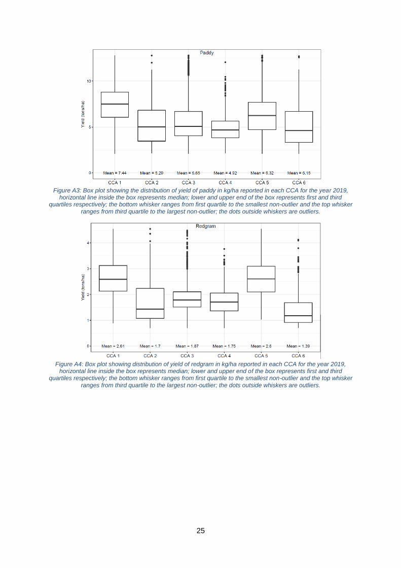
25

Figure A3: Box plot showing the distribution of yield of paddy in kg/ha reported in each CCA for the year 2019,



Figure A4: Box plot showing distribution of yield of redgram in kg/ha reported in each CCA for the year 2019,



Technical Assistance Consultant's Report - 42384-012 ...

Documents

Transcript of Technical Assistance Consultant's Report - 42384-012 ...