Value Matters:

Predictability of Stock Index Returns

Natascia Angelini∗1, Giacomo Bormetti†2, Stefano Marmi‡3, and Franco Nardini§4

1MEDAlics, Dante Alighieri University

Via del Torrione 95, 89125 Reggio Calabria, Italy

School of Economics, Management and Statistics, University of Bologna

Via Anghera 22, 40127 Rimini, Italy

2Scuola Normale Superiore

Piazza dei Cavalieri 7, 56126 Pisa, Italy

3Scuola Normale Superiore

Piazza dei Cavalieri 7, 56126 Pisa, Italy

4Department of Mathematics, University of Bologna,

Viale Filopanti 5, 40126 Bologna, Italy

Abstract

We present a simple dynamical model of stock index returns which is grounded on the

ability of the Cyclically Adjusted Price Earning (CAPE) valuation ratio devised by Robert

Shiller to predict long-horizon performances of the market. More precisely, we discuss a

discrete time dynamics in which the return growth depends on three components: i) a

momentum component, naturally justified in terms of agents’ belief that expected returns

are higher in bullish markets than in bearish ones, ii) a fundamental component propor-

tional to the logarithmic CAPE at time zero. The initial value of the ratio determines

∗Electronic address: natascia.angelini@unibo.it†Electronic address: giacomo.bormetti@sns.it‡Electronic address: stefano.marmi@sns.it§Electronic address: franco.nardini@unibo.it; Corresponding author, mobile phone: +39 335 8024631

1

the reference growth level, from which the actual stock price may deviate as an effect of

random external disturbances, and iii) a driving component which ensures the diffusive

behaviour of stock prices. Under these assumptions, we prove that for a sufficiently large

horizon the expected rate of return and the expected gross return are linear in the initial

logarithmic CAPE, and their variance goes to zero with a rate of convergence consistent

with the diffusive behaviour. Eventually this means that the momentum component may

generate bubbles and crashes in the short and medium run, nevertheless the valuation

ratio remains a good reference point of future long-run returns.

JEL codes: G12, G17

Keywords: Valuation Ratios, Long Run Stock Market Returns

1 Introduction

A question that has been asked with a certain regularity since the establishment of the first

stock index is the following, see Myers and Swaminathan (1999): is it possible to calculate “the

Intrinsic Value of the Dow”? Or, more generally: what is the intrinsic value of Wall Street? A

first commonsense answer is that this value may be calculated by summing “the intrinsic value”

of each quoted company. At the beginning of the past century, see Williams (1938), Graham

and Meredith (1998), it was well known that the latter depends on the expected future earnings

and on the balance sheet, but unfortunately there was no easy formula, which yielded even a

rough approximation. Therefore aggregating all expectations for all companies quoted in the

market soon appeared to be a challenging task.

Between the Fifties and the Sixties the researchers’ attitude towards the problem changed

radically. Modern portfolio theory and the statistical evidence that stock prices follow ran-

dom walks, see Mandelbrot (1965), Fama (1965), has led to the Efficient Market Hypothesis,

see Samuelson (1965), Fama (1970). According to this theory, financial markets are “informa-

tionally efficient”, that is, one can not achieve returns in excess of average market returns on

a risk-adjusted basis, given the information available at the time the investment is made. If

this were the case “the intrinsic value” of a stock would be simply its market price and the

problem would ultimately be non existent. The bubble burst in 1987 and the exceptional price

boom in the late ’90 lead more and more researcher to cast doubts on the hypothesis’ truth.

2

At the very beginning of 2000 Robert Shiller wrote: “we do not know whether the market level

makes any sense, or whether they are indeed the result of some human tendency that might be

called irrational exuberance”, Shiller (2000), which is apparently at odds with the assumption

that market prices are always fair prices. Shiller’s skeptical attitude was anticipated in one of

the most famous books ever written on the stock market: in 1934, Graham and Dodd strongly

advocated the fundamental approach to investment valuation and recommended to “shift(s)

the original point of departure, or basis of computation, from the current earnings to the av-

erage earnings, which should cover a period of not less than five years, and preferably seven

to ten years” Graham et al. (1962). Since 1988 Campbell and Shiller have been focusing their

attention on average earnings as predictor of future dividends Campbell and Shiller (1988a) 1

and future stock prices Campbell and Shiller (1998) 2; Shiller (2000) proposed an innovative

test of the appropriateness of prices in the stock market: the Cyclically Adjusted Price Earning

ratio, and showed that it is a powerful predictor of future long run performances of the market;

the performance of the test is quite satisfactory in the case of the US market from the end of

19th century up to today. In the same years, again elaborating on Graham et al. (1962), Lander

et al. (1997) suggested an alternative but similar criterion based on the assumption “that many

investors are constantly making a choice between stock and bond purchases; as the yield on

bonds advances, they would be expected to demand a correspondingly higher return on stocks,

and conversely as bond yields decline Graham et al. (1962, pag. 510)”; their “approach consid-

ers whether stocks are appropriately valued relative to analysts’ perceptions of future earnings

and yields on alternative investments” such as high grade corporate bonds (for a comparison

between the two approaches see Weigand and Irons (2006)).

The aim of this paper is to provide a theoretical framework which explains how future stock

index returns depend on the CAPE ratio. This is achieved by constructing a model. What we

require of our model is similar to what Chiarella required in Chiarella (1992, see pag. 102)

“Firstly we require that the model generate a significant transitory component around the

equilibrium which reflects the rationally expected value of the asset. Secondly the model must

1“Our results indicate that a long moving average of real earnings helps to forecast future real dividends.The ratio of this earnings variable to the current stock price is a powerful predictor of the return on stock,particularly when the return is measured over several years”.

2The price-smoothed earnings ratio has little ability to predict future growth in smoothed earnings; the Rsquared statistics are less than 4% over one year and over ten years. The ratio is a good forecaster of ten-yeargrowth in stock prices, with an R squared statistic of 37%.

3

allow for the incorporation of chartists, a group which bases its market actions on an analysis

of past trends. Since this group seems to be an important part of real markets it is important

to determine what effect its activity has on the behaviour of asset prices and whether the

behaviour of a model incorporating chartists comes closer to explaining some of the empirical

results cited earlier”.

We choose, however, a different approach and we work at an aggregate level instead of

explicitly modelling two different types of agents. We introduce a moment component in a

“simple error-correction model that predicts the return of the S&P based on the deviations

from a presumed equilibrium between . . . earnings yields” Lander et al. (1997, see pag. 3) and

a long run target yield rate. The return growth depends on three components

a) a momentum component, naturally justified in terms of agents’ expectation that expected

returns are higher in bullish markets than in bearish ones;

b) a fundamental component, proportional to a function of the level of the logarithmic

averaged earnings-to-price ratio (for brevity log EP ratio) at time zero; the initial time

value of log EP ratio determines the reference growth level, from which the actual stock

price may deviate as an effect of random external disturbances;

c) a driving component ensuring the diffusive behaviour of stock prices.

Under these assumptions, we are able to prove that, if we consider a sufficiently large number

of periods, the expected rate of return and the expected gross return are linear in the initial

time value of log EP, and their variance converges to zero with rate of convergence equal to

minus one. This means that, in our model, the stock prices dynamics may generate bubbles

and crashes in the short and medium run, nevertheless the averaged earnings-price ratio is a

good predictor of future long-run returns, as claimed by Campbell and Shiller (1988a), Shiller

(2000), Lander et al. (1997). The result holds for both returns and gross returns; in the latter

case we assume that the log dividend-to-price ratio follows a stationary stochastic process as

in Campbell and Shiller (1988a,b). Relaxing this assumption Engsted et al. (2012) have recently

investigated a model where explosive bubbles may arise, while Campbell (2008) has set forth

an innovative approach to estimate the equity risk premium.

In section 2 we review the econometric issues arising in when a rate of return is regressed on

4

a lagged stochastic regressor where the regression disturbance is correlated with the regressor’s

innovation. In section 3 we describe the data set we are going to use in the estimation of

the model. Section 4 sets up the model and derives the theoretical results. In section 5 we

estimate the parameters of our model for both the Standard and Poor Composite Stock Price

Index and the NYSE/AMEX value weighted index, and we present the results of a Monte Carlo

simulation, which confirms the ability of the proposed model to capture the relevant features of

the historical time series. Section 6 concludes. Technical proofs are gathered in the appendix.

2 Econometric framework

The approach that we discuss in this paper is based on the advances achieved in recent years

by different authors to deal with persistent regressions. Although the methodology that we

employ is of general applicability, we detail it with a specific focus on the topic of index returns

predictability with respect to valuation ratios.

We refer to the real (inflation adjusted) price of the stock index, measured at the beginning

of time period t, with Pt, while the notation Dt corresponds to the real dividend paid on the

portfolio during the period between t and t+ 1. Accordingly, we write the real log gross return

on the index held from the beginning of time t and the beginning of time t+ 1 as

Ht = log (Pt+1 +Dt)− logPt .

We provide a description of the return dynamics on a monthly basis. Therefore, the notation

t+ 1 refers to the time instant t increased by one month and the real gross yield over a period

of length h months corresponds to

yt,h =1

h

h−1∑

i=0

Ht+i . (1)

We also introduce the index log price pt = logPt, in terms of which the gross yield can be

5

rewritten as

yt,h =1

h

h−1∑

i=0

(pt+i+1 − pt+i) +1

h

h−1∑

i=0

log

(1 +

Dt+i

Pt+1+i

), (2)

where the first term on the right hand side is equivalent to (pt+h − pt)/h. The dependent

variable that we study throughout the paper is the gross return of the stock index, while the

regressor that we consider is the log Earnings-to-Price ratio (log EP) xt.= log 〈e〉10t − pt. The

quantity 〈e〉10t refers to a moving average of real earnings over a time window of ten years. At

variance with Campbell and Shiller (1988b), where the analysis is based on geometrical aver-

ages, we employ arithmetical averages. The very reason is that in this way our study can be

extended to the case of negative earnings. Indeed, while it is quite unrealistic that an average

over ten years results in a negative value, however it is not so uncommon to deal with spot

negative earnings. In this latter case the definition of log et would be problematic. Moreover,

we expect that switching from one average to the other does not significantly change the overall

picture. The use of an average of earnings in computing the ratios has been strongly pushed

by the literature in recognition of the cyclical variability of earnings. In Graham et al. (1962)

the authors recommend an approach that “Shifts the original point of departure, or basis of

computation, from the current earnings to the average earnings, which should cover a period

of not less than five years, and preferably seven to ten years.”

We assume that the return yt3 and the predictor satisfy the relations which follow

yt = α + β xt−1 + ut , (3)

xt = θ + ρ xt−1 + vt , (4)

where the errors (ut, vt) are serially independent and identically distributed as bivariate nor-

mal, with zero mean and covariance matrix Σ. We follow the same formal model of Stambaugh

(1999) where the time series of returns {yt} for t = 1, . . . , n is to be predicted by a scalar

first-order autoregressive time series {xt} for t = 0, . . . , n − 1. When the regressions of the

above type involve financial ratios the Ordinary Least-Squares (OLS) estimator for α and β is

3To ease the notation from the remaining of this section we express the log return yt−1,1 as yt.

6

biased in finite samples. This problem is pointed out by many authors, see for instance Mankiw

and Shapiro (1986), Stambaugh (1986), and is analyzed by Stambaugh (1999) who develops

an expression for the bias of the estimated prediction coefficient. In Stambaugh’s words “An

assumption that typically fails to hold (. . . ) is that ut has zero expectation conditional on

{. . . , xt−1, xt, xt+1, . . .}, and this is the assumption used to obtain finite-sample results in the

standard setting.” Stated in different words, the behaviour of ut is mainly determined by the

values pt−1 and pt so E(ut|xt, xt−1) 6= 0. Moreover, the dynamics of xt is strongly persistent

and largely influenced by the behaviour of pt. When the log price pt−1 increases, the idiosyn-

cratic term ut increases too, while vt decreases; the converse is true when the price decreases.

Empirically the value of ρ is relatively close to one and as an overall effect this induces a

strong anti-correlation between ut and vt. When both the endogeneity of the regression and

the persistence of xt are taken into account the high statistical significance of the standard OLS

estimator, βOLS, found in Campbell and Shiller (1987, 1988a,b) is to be questioned. However,

starting from Stambaugh (1999), Lewellen (2004) finds some evidence for predictability with

valuation ratios. This result relies on the upper bound for the bias in β which derives from

the conservative assumption that the autoregressive coefficient is very close to one. We follow

the alternative approach discussed in Amihud and Hurvich (2004). Replacing the predictive

regression (3) with the augmented regression

yt = αc + βcxt−1 + φcvct + et , (5)

where

vct = xt − θc − ρcxt−1 , (6)

it is possible to show that the OLS estimator of βc is a low-biased estimator of the true parameter

β appearing in (3). The quantities θc and ρc needed to define the regressor vct correspond to

reduced-bias estimators of θ and ρ, respectively. A possible choice for ρc corresponds to the

Kendall’s low-bias estimator of the AR(1) coefficient discussed in Kendall (1954). At variance

we employ the second-order bias corrected estimator proposed in Amihud and Hurvich (2004)

7

which reads

ρc = ρOLS +1 + 3ρOLS

n+ 3

1 + 3ρOLS

n2, (7)

where ρOLS is the standard OLS estimator. Coherently, the following relation holds

θc = (1− ρc)∑n−1

t=0 xtn

, (8)

with n equal to the number of available observations. The statistical significance of β can be

tested by means of a low-bias finite sample approximation of the standard error of βc which

deviates from the error provided by the OLS regression. The reason for this deviation is that

the OLS estimate fails to take into account the additional variability of βc due to the variability

of ρc. Unfortunately, within the same framework it seems not possible to derive an expression

for the error associated with α. Testing their approach on a data sample of monthly records

from the NYSE inflation-adjusted value-weighted index ranging from May 1963 to December

1994, Amihud and Hurvich find a highly statistically significant predictability for dividend

yields. In the present paper we perform the estimation of the α and β coefficients exploiting

the same methodology. However, as far as testing is concerned, we do not exclusively rely on

the t-statistic but we resort to a bootstrap approach which does not rely on any distributional

assumption for the residual components ut and vt. As we will show in section 5 we find coherent

results which support the forecasting ability of the logarithmic CAPE for both the Standard

and Poor and NYSE/AMEX market returns.

Before we move to the description of the bootstrap algorithm, it is worth to mention some

interesting alternative results dealing with the subtle issue of predictability with valuation ra-

tios. To the best of our knowledge, the most recent advance corresponds to Hjalmarsson (2011)

which is inspired by the testing framework discussed in Campbell and Yogo (2005, 2006). Both

approaches are grounded on the quasi-unit root approximation for the AR(1) coefficient of

equation 4, but while the latter focuses on short-run horizons the former extends the results to

arbitrary horizons. The extension to the long-run predictability involves a new element that

contributes to increase the complexity of the econometric issue. Indeed, long-run performances

8

can be evaluated only aggregating returns over smaller time scales. Given the intrinsic scarcity

of data points, the sample can be enlarged only resorting to overlapping realizations and in-

ducing sizable serial correlation among the residual terms. This side-effect can be managed

by means of auto-correlation robust estimators, for instance those discussed in Hansen and

Hodrick (1980), Newey and West (1987), however, when the correlation is particularly strong,

these methods show poor small sample properties as discussed in Hodrick (1992), Nelson and

Kim (1993). On the other hand the new asymptotic results developed in Hjalmarsson (2011)

are based on the scaling properties of the t-statistics and are tested on a sub sample of the data

used in Campbell and Yogo (2006) providing consistent results and evidence of the predictive

power of the logarithmic CAPE.

The bootstrap in the context of returns predictability is discussed in various papers, Kilian

(1999), Goyal and Santa-Clara (2003), Welch and Goyal (2008), and more specifically for re-

gressions based on valuation ratios in Maio (2012). The testing environment that we design

goes through the following steps:

i) We estimate the bias-corrected ρc and θc by means of (7) and (8). Using both values we

compute (6) and perform the augmented regression (5). We store the values αc and βc

that we find via OLS.

ii) We consider the regression (3) and (4) under the null hypothesis β = 0 and we estimate

the coefficients via OLS. We save the values α, θ, and ρ together with the sequence of

bivariate residuals (ut, vt) for t = 1, . . . , n.

iii) We sample b = 1, . . . , 104 bivariate sequences (ubt , vbt ) with t = sb1, . . . , s

bn. The time in-

dices sb1, . . . , sbn are sampled with replacement from the original set of indices t = 1, . . . , n.

iv) For each replication b = 1, . . . , 104, we compute a bootstrap sample by imposing the null

hypothesis

ybt = α + ubt ,

xbt = θ + ρxbt−1 + vbt .

9

The initial point xb0 is drawn uniformly from the set {xt}t=0,...,n−1.

v) For each bootstrap sample we estimate the bias-corrected θc,b and ρc,b, we compute the

proxy for the error terms vc,bt as

vc,bt = xbt − θc,b − ρc,bxbt−1 ,

and we estimate the following augmented regression via OLS

ybt = αc,b + βc,bxbt−1 + φc,bvc,bt + ebt .

Finally we obtain a sample{βc,b}

for b = 1, . . . , 104.

vi) The one sided p-value associated with the prediction coefficient is calculated as

p− value =#{βc,b > βc}

104,

where the numerator on the right hand side denotes the number of bootstrap estimates

higher than the original value, and we implicitly assume that βc > 0.

3 Data set

The data set analyzed in this paper consists of records on a monthly basis of prices, earnings,

and dividends for two stock price indexes for the US market. The first is the Standard and Poor

Composite Stock Price Index (S&P) data discussed in Campbell and Shiller (1987, 1988a,b), and

freely available from Robert J. Shiller’s webpage http://www.econ.yale.edu/. These time series

cover the entire period from January 1871 until December 2012. The second is NYSE/AMEX

value weighted index data (1926-1994) from the Center for Research in Security Prices (CRSP)

available from J. Campbell home page http://scholar.harvard.edu/campbell/data. Since earn-

ings data are not available for CRSP series we use the corresponding S&P earnings-to-price

ratios from Shiller. Figure 1 in Campbell and Yogo (2006) compares the time series of the

log dividend-to-price ratio for the NYSE/AMEX value-weighted index and the log smoothed

earnings-price for the S&P and provides support for our choice.

10

4 The model

In the current section we characterise a simple dynamical system driven both by a value in-

vestment and a momentum component. In the first instance we consider only the role played

by stock prices, but later we take into account gross returns and the effect of dividends. Our

model rests on the two assumptions which follow.

Assumption 1 Financial returns are naturally driven by the growth rate µt, and by an ancil-

lary process ξt satisfying

ξt+1 = ξt +κ

1− γσpWpt , (9)

with initial time condition ξ0 = 0. The ξt process ensures the diffusive behaviour of stock prices.

As will be clear later, the positive parameter σp corresponds to the long run returns volatility,

while the prefactor depending on κ > 0 and 0 < γ < 1 has been added for future convenience.

The W pt ’s for t = 0, . . . , h are independent identically distributed (i.i.d.) standard Gaussian

increments.

Assumption 2 The dynamics of log returns’ growth rate is given in terms of the difference

equation

µt+1 = γµt + κ[log〈e〉10t − pt + H + gF

(log〈e〉100 − p0

)t]

+ σµWµt (10)

where the parameter σµ is a positive volatility constant, and the W µt ’s for t = 0, . . . , h are i.i.d.

standard Gaussian increments, not dependent on the W pt ’s. The return growth µt depends on

its own value in the previous period, with γ agents’ sensitivity to market trend. This momentum

effect can be naturally justified in terms of agents’ expectation that returns are higher in bullish

markets than in bearish ones. The “fundamental” component is proportional to a function F of

the level of the logarithmic averaged earnings-to-price ratio at time zero, where the proportional-

ity constant is given by the rate of earnings growth g, implicitly defined by 〈e〉10t = 〈e〉100 exp (gt).

This component grows linearly with time, but we also allow for a correction equal to H, possibly

function of the initial time log EP ratio. The initial time value of log EP determines the refer-

11

ence growth level, from which the actual stock price may deviate as an effect of random external

disturbances. Investors reallocate assets in response to this disequilibrium causing stock prices

to move in the direction that reduces the deviation. The full adjustment is not immediate but

it takes a typical time κ−1 the price to mean revert to the fundamental level.

In conclusion, our model states the dynamics of log prices can be fully specified by the linear

stochastic difference system

pt+1 = pt + µt + ξt

µt+1 = γµt + κ (log〈e〉10t − pt + H + gFt) + σµWµt

ξt+1 = ξt + κ1−γσpW

pt

, (11)

with p0 = logP0 and µ0 initial time conditions. By a further change of variable Yt = pt−log〈e〉100 ,

the expected values E0[Yt], E0[µt], E0[ξt] conditional at the information available at time 0 evolve

according to the linear first order difference system

E0[Yt+1] = E0[Yt] + E0[µt] + E0[ξt]

E0[µt+1] = −κE0[Yt] + γE0[µt] + κH + κg(1 + F)t

E0[ξt+1] = E0[ξt]

,

with the initial conditions

E0[Y0] = p0 − log〈e〉100E0[µ0] = µ0

E0[ξ0] = 0

.

Lemma 1. The expected rate of return is linear in F(log〈e〉100 − p0), provided we consider a

sufficiently large number of periods h

E0

[1

hlog

P0+h

P0

]= g(1 + F) +O(

1

h) . (12)

Moreover its variance converges to zero with rate of convergence equal to minus one

V ar0

[1

hlog

P0+h

P0

]=σ2p

h+ o(

1

h) . (13)

12

A posteriori it is clear why we fixed the proportionality constant of the fundamental compo-

nent equal to g. Indeed, in case g were zero not only averaged earnings but also stock returns

would grow sub-exponentially. The variance of Yh increases linearly with h, the diffusive be-

haviour of stock returns that any realistic model should satisfy in a first instance. Finer effects,

like possible return non zero autocorrelations induced by business cycles over long horizons

could be included in our model modifying the covariance structure of the {W pt } noise. In this

respect it is worth to remark that none of our results crucially rest on the Gaussian assumption

for the noise increments.

From previous Lemma the result that we state below follows.

Corollary 2. If F is linear in log〈e〉100 − p0, than the model (11) is able to reproduce the linear

scaling of returns with the initial log EP ratio on the long run.

The next step forward is to add a dividend components to our stock returns model. In this

respect we mainly follow the proposal discussed in Campbell and Shiller (1988a,b), where it

is argued that the log dividend-to-price ratio follows a stationary stochastic process, and the

fixed mean of logDt − logPt, logG, can be used as an expansion point

∆(dt−1 − pt) = −θ(dt−1 − pt − logG) + σdWdt , (14)

with dt = logDt, σd > 0, and {W dt } for t = 1, . . . , h i.i.d. standard Gaussian variates. At

variance with the proposal of Campbell and Shiller, we also assume that G can possibly depend

on the log EP at time zero, i.e. G = G(log〈e〉100 − p0).

Lemma 3. In the limit h� 1 the quantity 1h

∑h−1i=0 log

(1 + Di

Pi+1

)contributes to the rate of log

gross returns proportionally to G, and its variance converges to zero with rate minus one.

Corollary 4. If G is linear in log〈e〉100 − p0, than equation (14) is able to reproduce the linear

scaling of dividends’ contribution to the yield with the initial log EP ratio on the long run.

We are now ready to state the main theoretical result of this paper.

Preposition 5. The expected gross yield (1) is linear in F and G, provided we consider suffi-

ciently long horizons

E0[yh] ' g(1 + F) + G +O

(1

h

). (15)

13

The proof is an immediate consequence of the Corollaries 2 and 4. Interestingly from the

proofs of previous Lemmas given in Appendix (A) we can explicitely identify the contribution to

the long term yield whose scaling over time is more persistent, and which ultimately determines

its convergence towards the limit g(1 + F) + G. The expression of the leading correction

proportional to one over h reads

H− g(1 + F)

[1 + κ

1− λ−λ+(1− λ−)2(1− λ+)2

]+ logEP0 + G

(1− 1

θ

)(logDP0 − logG) . (16)

From equation (21) we know that (1−θ)t plays the role of a damping function. Assuming θ � 1,

it reduces to exp(−t/τθ) where the quantity τθ = 1/θ plays the role of the typical time scale

of the mean-reverting process. We reasonably expect that the last term in the expression (16)

does not contribute too much to the leading correction, since we neither expect an extremely

large time scale for the process nor an extreme discrepancy between logDP0 and logG. Another

interesting point to note is that the choice of µ0 plays a minor role in relation to the speed

of convergence of the process to the long term expected value. Indeed, µ0 does not appear in

expression (16), while from (19) we know that its effect is exponentially damped by λh− and

λh+. Being 0 < λ− < λ+ < 1, the dominating contribution for h � 1 is given by λh+, implying

a typical damping scale equal to −(log λ+)−1.

5 Parameters estimation

Corollaries 2 and 4 state that the linear scaling of long term yield with the level of log EP

ratio can be reproduced by our dynamical model if we assume for the quantities g(1 + F) and

G the form g(1 + F) = αF + βF log EP0 and G = αG + βG log EP0. Following the same approach

of Amihud and Hurvich (2004), we estimate the values of αF, βF from the regression of log

returns over one year horizon on the initial log EP. The quantities labelled with G are obtained

in the same way after regressing the dividends’ contribution to the yield on the same regressors.

The results that we find are reported in Table 1 for both the S&P and NYSE/AMEX indices.

We also report the prediction coefficients of the gross returns on the initial logarithmic CAPE,

α and β. The statistical significance of the β coefficients is assessed by means of the reduced-

biased standard errors discussed in Amihud and Hurvich (2004) and according to the bootstrap

14

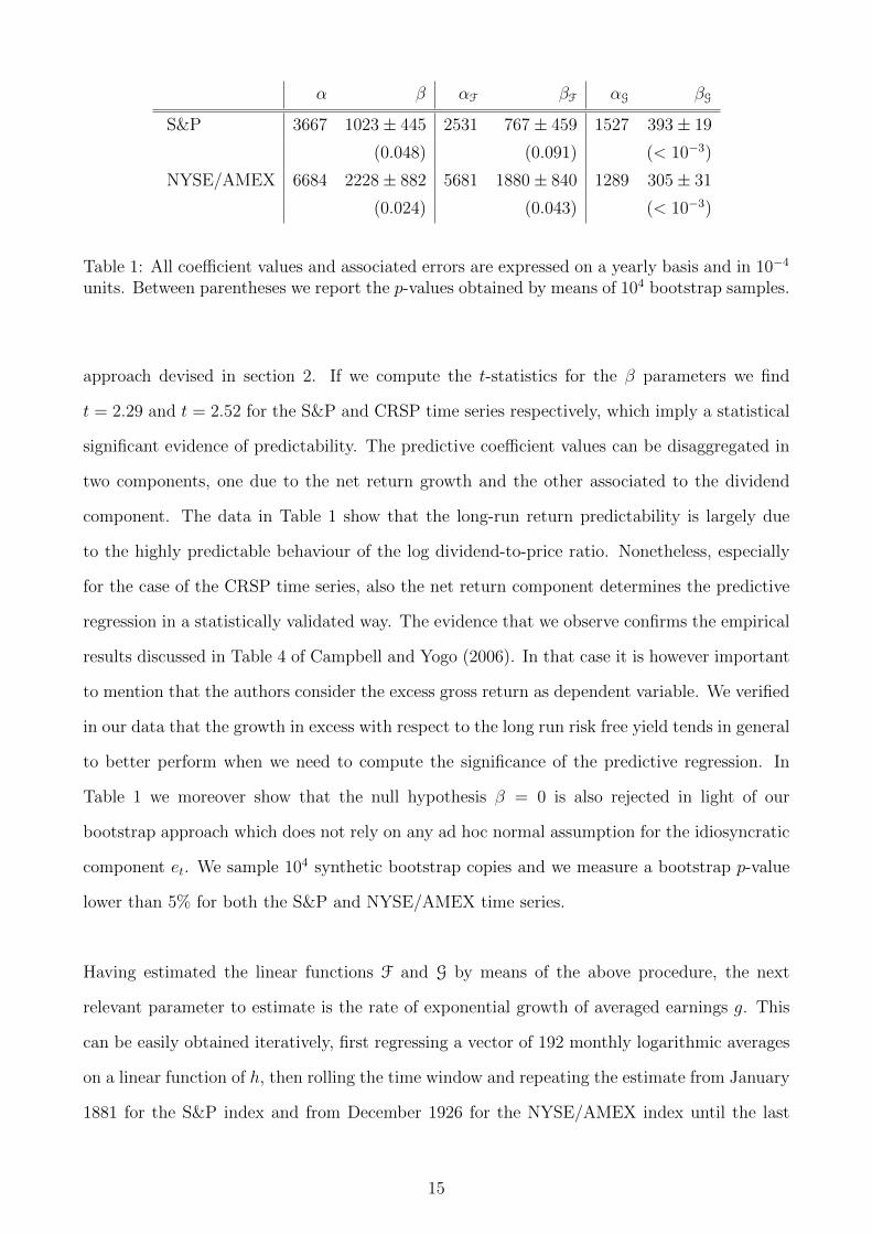
α β αF βF αG βG

S&P 3667 1023± 445 2531 767± 459 1527 393± 19

(0.048) (0.091) (< 10−3)

NYSE/AMEX 6684 2228± 882 5681 1880± 840 1289 305± 31

(0.024) (0.043) (< 10−3)

Table 1: All coefficient values and associated errors are expressed on a yearly basis and in 10−4

units. Between parentheses we report the p-values obtained by means of 104 bootstrap samples.

approach devised in section 2. If we compute the t-statistics for the β parameters we find

t = 2.29 and t = 2.52 for the S&P and CRSP time series respectively, which imply a statistical

significant evidence of predictability. The predictive coefficient values can be disaggregated in

two components, one due to the net return growth and the other associated to the dividend

component. The data in Table 1 show that the long-run return predictability is largely due

to the highly predictable behaviour of the log dividend-to-price ratio. Nonetheless, especially

for the case of the CRSP time series, also the net return component determines the predictive

regression in a statistically validated way. The evidence that we observe confirms the empirical

results discussed in Table 4 of Campbell and Yogo (2006). In that case it is however important

to mention that the authors consider the excess gross return as dependent variable. We verified

in our data that the growth in excess with respect to the long run risk free yield tends in general

to better perform when we need to compute the significance of the predictive regression. In

Table 1 we moreover show that the null hypothesis β = 0 is also rejected in light of our

bootstrap approach which does not rely on any ad hoc normal assumption for the idiosyncratic

component et. We sample 104 synthetic bootstrap copies and we measure a bootstrap p-value

lower than 5% for both the S&P and NYSE/AMEX time series.

Having estimated the linear functions F and G by means of the above procedure, the next

relevant parameter to estimate is the rate of exponential growth of averaged earnings g. This

can be easily obtained iteratively, first regressing a vector of 192 monthly logarithmic averages

on a linear function of h, then rolling the time window and repeating the estimate from January

1881 for the S&P index and from December 1926 for the NYSE/AMEX index until the last

15

(g) 14 Years

−6 −5 −4

log〈e〉10t − logPt

−0.05

0

0.05(h) 16 Years

−6 −5 −4

log〈e〉10t − logPt

(e) 10 Years

−0.05

0

0.05

1 h

∑h−1

i=0log

Pt+

i+

1+D

t+

i

Pt+

i

(f) 12 Years

(c) 6 Years

−0.05

0

0.05(d) 8 Years

1881

1891

19111931

1941

1951

19611981

2001

(a) 2 Years

1901

1921

1971 1991

−0.05

0

0.05(b) 4 Years

Figure 1: Monte Carlo scenarios generated simulating the model given by equations (11)and (14) with inital time conditions Y0, µ0, and logDP0 equal to the empirical ones. The dashedline corresponds to the long-run behaviour predicted by the equation (15) using the coefficientvalues of Table 1 for the S&P index rescaled to a monthly level. The dotted lines correspond tothe boundaries of the 95% confidence level region. Points are organised in chronological orderaccording to the color scale ranging from dark blue to red passing through light blue, green,yellow, and orange; labels in the top left panel refer to points which correspond to the firstmonth of the specified year.

16

admissible date. In this way we obtain a sample of g values from which empirical 68% confidence

intervals can be computed, for the results on a monthly basis from Shiller’s and Campbell’s data

series please refer to Table 2. The value of θ and σd are estimated regressing ∆(dt−1 − pt) on

dt−1−pt−logG, employing the same technique of rolling windows. The measured mean value for

θ is equal to 0.0271 and 0.0445 for the S&P and NYSE/AMEX index respectively, and following

the consideration written at the end of the previous section these values imply typical scales

for mean-reversion of order 37 and 22 months, respectively. The parameters of the µt process

are also estimated by means of linear regression of µt+1 on µt, and on log〈e〉10t − pt + H + gFt.

In the first instance this requires to introduce a suitable proxy for the unobservable variable

µt. Our approach is to estimate it by means of pt − pt−1, but different choices are admissible,

for example in terms of an exponential weighted average of past price returns. However in this

latter case the undesirable dependence of the parameters on the value of the exponential weight

would be introduced. Moreover H is still an unknown quantity that we have to choose before

performing the optimization procedure. Recalling expression (16), it is reasonable to assume it

linear in the log EP ratio H = αH + βH logEP0 and to initialise the procedure with arbitrary

values for the linear coefficients. The numerical process then produces optimal estimates of γ

and κ, for suitable αH and βH minimizing the leading correction term (16). In particular, for

αH = 0.85 and βH = −0.85 we find γ = 0.25 and κ = 0.03 for S&P, and for αH = 2.62 and

βH = −0.52 we find γ = 0.08 and κ = 0.03 for NYSE/AMEX, both satisfying the constraint

4κ 6 (1 − γ)2. For the estimate of σp we approach the problem from a different perspective.

Indeed from equation (13) we know that the variance of (ph − p0)/h scales as one over h with

proportionality constant equal to σ2p. We therefore fit the empirical curves with a linear relation

and we find the values of 0.182% and 0.168% reported in Table 2. In Figure 1 we present the

results of a Monte Carlo simulation of the model (11)-(14). Each point corresponds to a single

realization of yt,h with h = 24, . . . , 192 months with t starting from January 1881. The initial

time values of Y0, µ0, and logDP0 are fixed equal to the empirical ones. We plot the linear

relation between yields and the log EP as predicted by the equation (15) using the coefficient

values of Table 1 for the S&P index rescaled to a monthly level. We also provide the boundaries

of the 95% confidence level region which we compute by means of the formulas (13) and (22).

All the analytical predictions are fully confirmed by the Monte Carlo numerical results.

17

S&P NYSE/AMEX

g (×10−4 month−1) 12 (−3, 31) 19 (4, 32)

θ (×10−4 month−1) 271 (111, 430) 445 (197, 780)

γ 0.25 (0.18, 0.33) 0.08 (0.02, 0.15)

κ (×10−4 month−1) 323 (81, 597) 304 (70, 547)

σ2d (×10−4 month) 13 (10, 20) 19 (13, 25)

σ2µ (×10−4 month) 12 (9, 18) 17 (12, 24)

σ2p (×10−4 month) 18.2 (18.1, 18.3) 16.8 (16.5, 17.1)

Table 2: Parameter values for the S&P and NYSE/AMEX time series with associated 68%confidence level intervals.

Finally, we test the goodness of the estimated parameters and the effectiveness of our dynamical

system. In Figures (2) and (3) we plot the prediction of equation (15) with the associated

confidence band on the net returns and on the gross yields, respectively, for time horizons

ranging from 24 to 192 months. As expected the model captures the shrinking of the historical

data cloud with a scaling exponent dominated by the diffusive component of the price dynamics.

As far as the central value is concerned, the consistency is very good for the short time horizons,

whilst it worsens for longer runs. This effect is partially expected, since the linear coefficients

of the predictive regressions are constants quantities which are exogenous to the dynamical

model (11) and do not evolve with time. We are currently working on an econometric approach

to the model (3)-(4) in order to provide a sound theoretical basis to the extension of the low-bias

procedure of Amihud and Hurvich (2004) to long-run horizons. Preliminary results suggest that

the β coefficient rescales geometrically over time, where the basis of the geometric sequence

corresponds to the AR(1) coefficient of equation (4). We plan to correct for this minor effect

in a future extension of our model.

6 Conclusion and Perspectives

This paper documents predictability of stock index returns for the U.S. market on the basis of

a simple valuation metric, the cyclically adjusted price-earnings ratio, and proposes a discrete

time dynamical model able to capture the long-run behaviour.

18

(g) 14 Years

−6 −5 −4

log〈e〉10t − logPt

−0.05

0

0.05(h) 16 Years

−6 −5 −4

log〈e〉10t − logPt

(e) 10 Years

−0.05

0

0.05

(pt+

h−pt)/h

(f) 12 Years

(c) 6 Years

−0.05

0

0.05(d) 8 Years

1881

1891

1911

1931

1941

19511961

1981

2001

(a) 2 Years

1901

1921

1971 1991

−0.05

0

0.05(b) 4 Years

Figure 2: Regression of the yield (pt+h − pt)/h on the explanatory log earning - price ratio.Solid points: empirical data, dashed line: model prediction, dotted line: 95% confidence levelfrom model prediction. Color scale as in Figure 1.

19

(g) 14 Years

−6 −5 −4

log〈e〉10t − logPt

−0.05

0

0.05(h) 16 Years

−6 −5 −4

log〈e〉10t − logPt

(e) 10 Years

−0.05

0

0.05

1 h

∑h−1

i=0log

Pt+

i+

1+D

t+

i

Pt+

i

(f) 12 Years

(c) 6 Years

−0.05

0

0.05(d) 8 Years

1881

18911911

1931

1941

19511961 1981

2001

(a) 2 Years

1901

1921

1971 1991

−0.05

0

0.05(b) 4 Years

Figure 3: Regression of yield (1) on the explanatory log earning - price ratio. Points, lines,labels, and color scale as in Figure 2.

20

Substantial evidence of the importance of fundamentals in the valuation of international stock

markets has been accumulated by the proponents of fundamental indexation Arnott et al.

(2005). Practitioners and academicians alike have been using several valuation measures for

estimating the intrinsic value of a stock index: for example in table 2 of Poterba and Samwick

(1995) the ratio of market value of corporate stock to GDP, the year-end price-to-earnings ratio,

the year-end price-to-dividend ratio and Tobin’s q are reported from 1947 to 1995 in an effort

of alerting the reader on the possible overvaluation of the index 4. In particular Tobin’s q has

been proposed as another efficient method of measuring the value of the stock market, with

an efficiency comparable to the CAPE Smithers (2009). The q ratio is the ratio of price to

net worth at replacement cost rather than the historic or book cost of companies. It therefore

allows for the impact of inflation, much alike the CAPE which averages real earnings over a ten

year span. It would be interesting to carry out an empirical analysis of the relationship between

Tobin’s q and future stock index returns as far as to extend the present approach to countries

other than the U.S.. Both perspectives are worth to be followed but require high quality long-

term time series which at the moment we have not been able to find. Longer time-series would

also be important so as to investigate possible “evolutionary” phenomena like the end of the

relationship between market valuation and interest rates, which may perhaps be interpreted as

an example of the adaptive market hypothesis Farmer and Lo (1999), Lo (2004).

References

Yakov Amihud and Clifford M. Hurvich. Predictive regressions: A reduced-bias estimation

method. Journal of Financial and Quantitative Analysis, 39(04):813–841, 2004.

Robert D. Arnott, Jason Hsu, and Philip Moore. Fundamental indexation. Financial Analysts

Journal, 61(2):83–99, 2005.

4“It is difficult to distill a simple conclusion from table 2. While price-to-earnings ratios are not unusually highat present, other measures of stock price valuation are at, or near, historical highs. (. . .) Table 2 does suggest,however, that in assessing the macroeconomic consequences of stock price movements, it may be importantto distinguish between stock price fluctuations that are associated with movements in the price-to-earnings orprice-to-dividends ratios and those that are not. A number of recent studies suggest that variations in theearnings-to-price ratio are correlated with prospective stock market returns, (. . .). Sharp increases in eitherthe price-to-earnings or the price-to-dividends ratio, other things equal, are associated with lower prospectivereturns.”

21

John C. Campbell. Viewpoint: Estimating the equity premium. Canadian Journal of Eco-

nomics / Revue Canadienne d’Economique, 41(1):1–21, 2008.

John Y. Campbell and Robert J. Shiller. Cointegration and tests of present value models.

Journal of Political Economy, 95(5):1062–1088, 1987.

John Y. Campbell and Robert J. Shiller. The dividend-price ratio and expectations of future

dividends and discount factors. Review of Financial Studies, 1(3):195–228, 1988a.

John Y. Campbell and Robert J. Shiller. Stock prices, earnings and expected dividends. Journal

of Finance, XLIII(3):661–676, 1988b.

John Y. Campbell and Robert J. Shiller. Valuation ratios and the long-run stock market

outlook. The Journal of Portfolio Management, 24(2):11–26, 1998.

John Y. Campbell and Motohiro Yogo. Implementing the econometric methods in efficient tests

of stock return predictability. Unpublished working paper. University of Pennsylvania, 2005.

John Y. Campbell and Motohiro Yogo. Efficient tests of stock return predictability. Journal of

financial economics, 81(1):27–60, 2006.

Carl Chiarella. The dynamics of speculative behaviour. Annals of Operations Research, 37(1):

101–123, 1992.

Tom Engsted, Thomas Q. Pedersen, and Carsten Tanggaard. The log-linear return approx-

imation, bubbles, and predictability. Journal of Financial and Quantitative Analysis, 47:

643–665, 2012.

Eugene F. Fama. The behavior of stock-market prices. The Journal of Business, 38:34–105,

1965.

Eugene F. Fama. Efficient capital markets: A review of theory and empirical work. Journal of

Finance, 25(2):383–417, 1970.

Doyne Farmer and Andrew W. Lo. Frontiers of finance: Evolution and efficient markets.

Proceedings of the National Academy of Sciences, 96(18):9991–9992, 1999.

22

Amit Goyal and Pedro Santa-Clara. Idiosyncratic risk matters! The Journal of Finance, 58

(3):975–1008, 2003.

Benjamin Graham and Spencer B. Meredith. The Interpretation of Financial Statements: The

Classic 1937 Edition. HarperBusiness, 1998.

Benjamin Graham, David L. Dodd, and Sidney Cottle. Security Analysis. McGraw-Hill, New

York, 1962.

Lars P. Hansen and Robert J. Hodrick. Forward exchange rates as optimal predictors of future

spot rates: An econometric analysis. The Journal of Political Economy, pages 829–853, 1980.

Robert J. Hodrick. Dividend yields and expected stock returns: Alternative procedures for

inference and measurement. Review of Financial studies, 5(3):357–386, 1992.

Erik Hjalmarsson. New methods for inference in long-horizon regressions. Journal of Financial

and Quantitative Analysis, 46(3):815, 2011.

Maurice G. Kendall. Note on bias in the estimation of autocorrelation. Biometrika, 41(3-4):

403–404, 1954.

Lutz Kilian. Exchange rates and monetary fundamentals: what do we learn from long-horizon

regressions? Journal of Applied Econometrics, 14(5):491–510, 1999.

Joel Lander, Athanasios Orphanides, and Martha Douvogiannis. Earnings forecasts and the

predictability of stock returns: Evidence from trading the S&P. Technical report, Board of

Governors of the Federal Reserve System, 1997.

Jonathan Lewellen. Predicting returns with financial ratios. Journal of Financial Economics,

74(2):209–235, 2004.

Andrew W. Lo. The adaptive markets hypothesis: Market efficiency from an evolutionary

perspective. Journal of Portfolio Management, 30(5):15–29, 2004.

Paulo Maio. The fed model and the predictability of stock returns. Review of Finance, 2012.

doi: 10.1093/rof/rfs025.

23

Benoit Mandelbrot. The variation of certain speculative prices. The Journal of Business, 36

(4):394–419, 1965.

Gregory N. Mankiw and Matthew D. Shapiro. Do we reject too often? : Small sample properties

of tests of rational expectations models. Economics Letters, 20(2):139–145, 1986.

James Myers and Bhaskaran Swaminathan. What is the intrinsic Value of the Dow? Journal

of Finance, 54(5):1693–1741, 1999.

Charles R. Nelson and Myung J. Kim. Predictable stock returns: The role of small sample

bias. The Journal of Finance, 48(2):641–661, 1993.

Whitney K. Newey and Kenneth D. West. A simple, positive semi-definite, heteroskedasticity

and autocorrelation consistent covariance matrix. Econometrica: Journal of the Econometric

Society, pages 703–708, 1987.

James M. Poterba and Andrew A. Samwick. Stock ownership patterns, stock market fluctua-

tions, and consumption. Brookings Papers on Economic Activity, 1995(2):295–372, 1995.

Paul Samuelson. Proof that properly anticipated prices fluctuate randomly. Industrial Man-

agement Review, 6(2):41–49, 1965.

Robert J. Shiller. Irrational Exuberance. Princeton University Press, 2000.

Andrew Smithers. Wall Street Revalued. Imperfect Markets and Inept Central Bankers. John

Wiley and Sons, Ltd, 2009.

Robert F. Stambaugh. Bias in regressions with lagged stochastic regressors. Center for Research

in Security Prices, Graduate School of Business, University of Chicago, 1986.

Robert F. Stambaugh. Predictive regressions. Journal of Financial Economics, 54(3):375–421,

1999.

Robert A. Weigand and Robert Irons. Does the market P/E ratio revert back to “average”?

Investment Management and Financial Innovations, 3(3):30–39, 2006.

Ivo Welch and Amit Goyal. A comprehensive look at the empirical performance of equity

premium prediction. Review of Financial Studies, 21(4):1455–1508, 2008.

24

John Burr Williams. The Theory of Investment Value. Harvard University Press, 1938.

A Proofs

Proof of Lemma 1. The stochastic dynamical system (11) may be put in the vector form

Vt+1 = JVt + κH e2 + κg(1 + F)t e2 + σµWµt e2 +

κ

1− γσpWpt e3 (17)

where J =

1 1 1

−κ γ 0

0 0 1

is the matrix of the systems, ei for i = 1, 2, 3 is the orthonormal

canonical base, and Vt =

Yt

µt

ξt

. The set of the eigenvalues of J includes 1, independently of

κ and γ, and two ones more

λ+ =γ + 1

2+

1

2

√(1− γ)2 − 4κ ,

λ− =γ + 1

2− 1

2

√(1− γ)2 − 4κ .

In order to ensure |λ+| < 1 and |λ−| < 1, we need to impose the following restrictions

0 < γ < 1 , and 0 < κ 6(1− γ)2

4. (18)

Iterating (17) we obtain

Vh = JhV0 + κ [g(1 + F)(h− 1) + H]h−1∑

k=0

Jke2 − κg(1 + F)h−1∑

k=0

kJke2

+σµ

h−1∑

k=0

W µk J

h−1−ke2 +κ

1− γσph−1∑

k=0

W pk J

h−1−ke3 .

25

We can rewrite more conveniently J = QΛQ−1 by means of the matrices Λ =

1 0 0

0 λ+ 0

0 0 λ−

,

Q =

1− γ 1 1

−κ λ+ − 1 λ− − 1

κ 0 0

, and Q−1 = 1|Q|

0 0 λ− − λ+κ(λ− − 1) −κ (1− γ)(1− λ−)− κ

κ(1− λ+) κ κ− (1− γ)(1− λ+)

with |Q| = κ(λ− − λ+). Taking expectation of et1Vh we obtain

E0 [Yh] = et1QΛhQ−1V0

+κ [g(1 + F)(h− 1) + H]h−1∑

k=0

et1QΛkQ−1e2

−κg(1 + F)h−1∑

k=0

ket1QΛkQ−1e2

= − λh+λ− − λ+

[(1− λ−)Y0 + µ0] +λh−

λ− − λ+[(1− λ+)Y0 + µ0]

+g(1 + F)(h− 1) + H

− [g(1 + F)−H]κ

λ− − λ+

(λh+

1− λ+− λh−

1− λ−

)

−g(1 + F)κ

λ− − λ+

[λ−

1− λh−(1− λ−)2

− λ+1− λh+

(1− λ+)2

]. (19)

From previous expression relation (12) immediately follows.

As far as the variance of Yh is concerned, we have

V ar0 [Yh] =h−1∑

k=0

[σ2µ

(et1QΛkQ−1e2

)2+

κ2

(1− γ)2σ2p

(et1QΛkQ−1e3

)2], (20)

from which we find

V ar0[Yh] =σ2µ

(λ− − λ+)2

h−1∑

k=0

[λk− − λk+

]2

+σ2p

(λ− − λ+)2

h−1∑

k=0

[λ− − λ+ + λk+(1− λ− −

κ

1− γ )

+λk−(κ

1− γ − 1 + λ+)

]2,

and the thesis (13) follows.

Proof of Lemma 3. On a monthly basis the quantity Dt/Pt+1 is of order 10−3, and we are

26

allowed to replace log(

1 + Dt

Pt+1

)with Dt/Pt+1. In the same spirit of Campbell and Shiller

(1988a,b), in order to prove the thesis we need to Taylor expand the quantities of interest

around logG. In particular, we have

Dt

Pt+1

= exp (dt − pt+1) ' exp (logG) (1 + dt − pt+1 − logG) .

Iterating equation (14) and taking expectation, we obtain for t > 0

E0[dt−1 − pt] = (1− θ)t(d−1 − p0) + logG[1− (1− θ)t

], (21)

where d−1 is the log dividend prevailing at time zero being cumulated between time -1 and

zero. Under the constraint 0 < θ < 2, we can conclude

1

hE0

[h−1∑

i=0

log

(1 +

Di

Pi+1

)]' G(1− logG) + G logG

+G1− θθ

(logDP0 − logG)1− (1− θ)h

h

= G +O

(1

h

),

and

V ar0

[1

h

h−1∑

i=0

log

(1 +

Di

Pi+1

)]' 1

h

G2σ2d

θ(2− θ) + o

(1

h

). (22)

Remark. The expansion performed in the above proof is similar to that proposed in Campbell

and Shiller (1988a,b), where log(Pt + Dt) is approximated by ϑpt + (1 − ϑ) logDt + κ with

ϑ = 1/(1 + G) and κ = log(1 + G)− ϑG logG.

27