Are Securitized Real Estate Returns more Predictable than Stock Returns?

Are Securitized Real Estate Returns more Predictablethan Stock Returns?

Camilo Serrano & Martin Hoesli

Published online: 15 November 2008# Springer Science + Business Media, LLC 2008

Abstract This paper examines whether the predictability of securitized real estatereturns differs from that of stock returns. It also provides a cross-country comparison ofsecuritized real estate return predictability. In contrast to most of the literature on thisissue, the analysis is not based on a multifactor asset pricing framework as such analysesmay bias the results. We use a time series approach and thus create a level playing fieldto compare the predictability of the two asset classes. Forecasts are performed withARMA andARMA–EGARCHmodels and evaluated by comparing the entire empiricaldistributions of prediction errors, as well as with a trading strategy. The results, based ondaily data for the 1990–2007 period, show that securitized real estate returns aregenerally more predictable than stock returns in countries with mature and wellestablished REIT regimes. ARMA–EGARCH models are found to have portfoliooutperformance potential even in the presence of transaction costs, with generally betterresults for securitized real estate than for stocks.

Keywords Predictability . Time series models . ARMA–EGARCH . REITs .

Securitized real estate

JEL Classifications C53 . C22 . G15

J Real Estate Finan Econ (2010) 41:170–192DOI 10.1007/s11146-008-9162-y

C. SerranoUniversity of Geneva (HEC), 40 boulevard du Pont-d’ Arve, CH-1211 Geneva 4, Switzerlande-mail: [email protected]

M. Hoesli (*)University of Geneva (HEC and SFI), 40 boulevard du Pont-d’ Arve, CH-1211 Geneva 4, Switzerlande-mail: [email protected]

M. HoesliUniversity of Aberdeen (Business School), Edward Wright Building, Aberdeen AB24 3QY Scotland,UK

M. HoesliBordeaux Ecole de Management (CEREBEM), F-33405 Talence Cedex, France

Introduction

After tripling in size over the past 5 years, the global market capitalization of realestate securities as measured by the FTSE EPRA/NAREIT Global Index amounts to$794 billion as of the end of 2007. The strong growth experienced by real estatesecurities may be largely attributed to the adoption of REIT-like legislation, i.e.legislation providing for tax-transparency at the corporate level, in an increasingnumber of countries. In 1995, REITs were only present in six countries, but by 2007,over 30 countries had introduced REIT regimes and several others were consideringsuch legislation. The explosion in REIT legislation reflects the increasing demandfor securitized forms of real estate and the consolidation of securitized real estate asan independent asset class. As such, it is important to examine the predictability ofsecuritized real estate returns, in particular whether these returns are more easilypredictable than stock returns. This paper uses a time series approach to forecastsecuritized real estate returns and compares their forecasting properties to those ofcommon stocks. For that purpose, we use daily returns for the 1990–2007 period.

Finding an asset class that is more predictable than another would changeinvestors’ perceptions concerning the uncertainty of future returns on that asset class,and therefore this could motivate important changes in terms of asset allocation. It ishard to determine a priori what results to expect from this study. On the one hand, itcould be argued that securitized real estate returns may be easier to forecast due tothe stable cash flows derived from the generally long-term leases. On the other hand,stock returns might seem more predictable than securitized real estate returns as thelatter are constituted by mid and small-cap companies whose returns are generallymore uncertain than those of larger companies.

Existing research has mainly compared the predictability of securitized real estate andstock returns by examining multifactor asset pricing models (Liu and Mei 1992; Meiand Liu 1994; Li and Wang 1995). However, two asset classes are not likely to beequally well specified by the same asset pricing model. Therefore, this type ofcomparison will not determine which asset class is more predictable per se, but whichasset class is more predictable under the asset pricing model specified. In other words,when multifactor asset pricing models are used, it is uncertain whether the similaritiesor differences in predictability are due to similarities or differences in predictabilitybetween the two asset classes, or to differences in the explanatory power of thespecified model for the two asset classes. To truly compare the predictability of twoasset classes, a ‘neutral’ model that does not favor any asset class should be employed.Such is the case of time series models as they rely solely on past observations and donot require the specification of forecasting variables. To the best of our knowledge,Nelling and Gyourko (1998) are the only to have used a time series approach tocompare the predictability between securitized real estate and stock returns.

This paper expands Nelling and Gyourko’s (1998) work by enriching theautoregressive-based analysis with ARMA and ARMA–EGARCH models. Further,the comparisons made are not evaluated merely with statistical criteria, but also byexamining entire empirical distributions as well as active trading strategies. Thisallows to conclude in a rigorous manner whether the returns of one of the two assetclasses are in fact more predictable than those of the other asset class, but also if theresults are economically significant. As the analysis covers ten countries, the

Are Securitized Real Estate Returns more Predictable than Stock Returns? 171

contribution of the paper is thus to provide a better understanding of the predictabilitybetween securitized real estate and stock returns at an international level, but also acomparison of the predictability of securitized real estate returns across countries.

The results of this study suggest that the maturity of the securitized real estatemarket plays an important role in the predictability of its returns. In countries withmature and well established REIT regimes, securitized real estate returns are foundto be more predictable than stock returns. Hence, the best forecasting accuracy isfound in the United States, the Netherlands, and Australia; the countries with theoldest REIT regimes in our sample. Furthermore, active trading strategies, especiallythose based on ARMA–EGARCH forecasts, are found to outperform the buy-and-hold benchmark in all ten countries for both asset classes. When transaction costs aretaken into account, this remains the case in half of our countries for real estatesecurities, but only in three for stocks.

The paper is structured as follows. The second section reviews the literature onthe forecasting of securitized real estate returns. The next section discusses the data,while the fourth section covers the methodology. Results are presented in the fifthsection and some concluding remarks follow.

Literature Review

Existing research on the forecasting of real estate returns (both direct andsecuritized) has relied on employing or comparing a number of univariate and/ormultivariate models. Univariate models have been found to perform well with directreal estate, while multivariate models have generally been preferred for securitizedreal estate. Although there is conflicting evidence in the literature as to whatforecasting technique works best, there is a general trade-off between the simplicityof the model and the forecasting accuracy.

Brooks and Tsolacos (2001) employ a number of time series techniques to assessthe predictability of securitized real estate returns in the U.K. They find that a VARmodel which incorporates financial spreads exhibits a better short-term out-of-sample forecasting performance than univariate time series models. However, afterestablishing trading rules with the forecasts, no excess returns are found over a buy-and-hold strategy once transaction costs are accounted for. In a follow-up paper,Brooks and Tsolacos (2003) compare the predictability of ARMA, VAR, and neuralnetworks models in five European countries. They conclude that whilst no singletechnique is universally superior, the neural networks model generally makes themost accurate predictions for 1-month horizons.

In the U.S., Serrano and Hoesli (2007) examine the usefulness of using financialassets, direct real estate, and the Fama and French (1993) factors to forecast EREITreturns and compare the predictive potential of time varying coefficient (TVC)regressions, VAR systems, and neural networks models. Their results indicate thatthe best predictions are obtained with neural networks models and especially whenthe model includes stock, bond, real estate, size, and book-to-market factors.Similarly in Australia, Ellis and Wilson (2005) find that portfolios constructed withneural networks techniques consistently out-perform the market on both a nominaland risk-adjusted basis. In the direct real estate literature, the performance of neural

172 C. Serrano, M. Hoesli

networks is less conclusive. The quality of the house price predictions obtained withthis technique is supported by some researchers (Nguyen and Cripps 2001;Limsombunchai et al. 2004; Peterson and Flanagan 2008), but criticized by others(Worzala et al. 1995; Lenk et al. 1997).

Existing research in the direct real estate market has addressed more thoroughlythe comparison of different forecasting techniques, especially in the U.S. and theU.K. Brown et al. (1997) suggest that the U.K.’s housing market is better forecastedwith a time-varying coefficient regression than with constant parameter ECMs, VARsystems or an autoregressive regression. In the U.S., Crawford and Fratantoni (2003)find that regime-switching models fit the data better than ARIMA or GARCHmodels. In spite of that, the performance of the simpler time-series models turns outto be as good or even better in out-of-sample tests. Analogously, Guirguis et al.(2005) compare the out-of-sample forecasts of six different estimation techniques.Their results indicate that the best forecasts are obtained with the rolling GARCHmodel and the Kalman filter with an autoregressive presentation (KAR) for theparameters’ time variation. Miles (2008) considers several non-linear models andfinds that generalized autoregressive (GAR) models generally do a better job at out-of-sample forecasting than ARMA and GARCH models, especially in markets withhigh home price volatility. In the Finnish office market, Karakozova (2004)compares the forecasting accuracy of a regression model, an ECM, and anARIMAX. The ARIMAX provides the best predictions when it incorporates laggedvalues of capital growth and contemporaneous values of growth in service sectoremployment and in the gross domestic product.

The literature comparing the predictability of REIT returns versus that of otherassets is filled with conflicting evidence. Liu and Mei (1992) use a multifactor latentvariable model with time-varying risk premiums and conclude that expected excessreturns are more predictable for EREITs than for stocks or bonds. These findings arealso confirmed by Liao and Mei (1998). However, Mei and Lee (1994) include a realestate factor to an otherwise similar multifactor asset pricing model and find noevidence of higher predictability for EREIT returns. Li and Wang (1995) also usesuch a framework to compare the returns of EREITs and MREITs to the returns ofstocks of other industries. Their findings suggest that the predictability of REITreturns is about the same as that of stocks. This multifactor asset pricing frameworkis examined out-of-sample by Mei and Liu (1994). They construct active tradingstrategies and find that larger profits and higher average risk-adjusted returns aregenerally obtained with EREITs than with other financial assets. Even though all ofthe preceding studies use the same framework, the lack of convergence in theirresults may be explained by the different model specifications employed. The threestudies suggesting more predictability for EREITs use the same forecastingvariables, i.e. the yield on a 1-month T-bill, the yield spread between AAA bondsand the T-bill, the dividend yield on an equally weighted portfolio, and thecapitalization rate on EREITs, whereas the two studies suggesting similarpredictability between the two asset classes use somewhat different forecastingvariables in the specification of their models.

The returns of an asset class may only be defined as more predictable than thoseof another asset class if the framework used does not create a disparity between thetwo asset classes with respect to the model specification. As such, a time series


approach creates the perfect conditions for such a comparison. This approach reliessolely on past observations and does not require the choosing of forecastingvariables that could bias the results by creating a model specification that is notequally fit for both asset classes. Nelling and Gyourko (1998) are the only authors tohave addressed this issue using a time series approach. Using AR processes to makethe forecasts and evaluating the out-of-sample predictability by employing acontrarian strategy, they find that small cap stocks are more predictable thanEREITs, but that EREITs are equally predictable as mid caps. However, their resultssuggest that the predictability of monthly EREIT returns is limited as it is not largeenough to cover transaction costs.

Performance continuation and reversals are also related to the time seriesproperties of asset returns and have been the subject of many studies in the financialeconomics literature. For securitized real estate, Mei and Gao (1995) examine serialpersistence of weekly returns and find that a contrarian-based strategy may beexploited only if transaction costs are ignored. Using a filter-based rule, Cooper et al.(1999) show that a contrarian strategy is in many cases more profitable than itsassociated execution costs. Graff and Young (1997) use different frequencies in theirstudy and find positive momentum effects with yearly data, evidence of performancereversals with monthly data, and no evidence of momentum or reversals withquarterly data. Finally, Stevenson (2002) provides international evidence ofmomentum effects over short and medium term horizons, as well as little supportfor price reversals.1

In sum, the existing literature on the predictability of securitized real estate returns hasconcentrated on comparing the predictability of different forecasting techniques and oncomparing the predictability of securitized real estate returns to that of other assetclasses. Concerning the various forecasting techniques, no single technique has beenfound to be universally superior although a general trade-off between the simplicity ofthe model and the forecasting accuracy has been acknowledged. Concerning thecomparisons of predictability between asset classes, the conclusions are mixed. This isnot surprising since the research examining this issue uses variations of the multifactorasset pricingmodel of Liu andMei (1992). Since a multifactor asset pricing model doesnot explain the returns of two asset classes to the same degree of accuracy due to thedifferent factors driving the returns of each asset class, the conclusions reached bythese studies are only valid for the multifactor asset pricing models being considered.Such criticism is not valid when time series models are considered as they do not favorone asset class over another as a result of the return generating model specified. Thus,this paper contributes to the literature by offering a more trustworthy comparison ofthe predictability of securitized real estate and stock returns.

Data

Whereas financial research customarily relies on daily data, empirical real estateresearch using securitized data has mainly concentrated on monthly, quarterly, and

1 For studies related to these issues in the direct real estate literature, see Young and Graff (1996, 1997) forthe U.S., Graff et al. (1999) for Australia, and Lee and Ward (2001) and Devaney et al. (2007) for the U.K.


yearly frequencies. However, the use of daily data is interesting for forecastingpurposes as the cost and time needed to collect and process information in real estatemarkets may be such that the market may be inefficient at daily frequencies, butefficient at monthly or lower frequencies (Mei and Gao 1995). Therefore, this paperuses daily total return indices for the period January 1990–December 2007.2

The data employed in this study were obtained from Thomson Datastream and theperiod selected was dictated by the starting date of the FTSE EPRA/NAREIT database.We cover the ten largest real estate security markets according to the FTSE EPRA/NAREIT Global Index. The overall market value of firms encompassed by the index is$794 billion; with the ten largest constituent countries representing approximately 95%of the index. These countries are the U.S., Hong Kong, Japan, Australia, the U.K.,France, Singapore, the Netherlands, Germany, and Sweden. For each country, we usethe relevant FTSE EPRA/NAREIT index. For stocks, Datastream’s total return indicesare used and, for the risk free rate, the Euro-Currency 3-month middle rate is retained.3

For Hong Kong, Australia and Sweden, the Euro-Currency rate is not available since1990, so the Interbank 3-month middle rate is used for the former two countries andthe Treasury Bill 90 day middle rate for the latter.

Since securitized real estate markets differ from country to country and suchdifferences may have significant effects on the degree of predictability of returns, anoverview of the markets is presented in Table 1. Albeit all the countries with theexception of Sweden had introduced REIT legislation by the end of 2007, only theU.S., the Netherlands, and Australia have REITs during the whole study period. Notsurprisingly, these three countries also have the highest percentage of REITs andtherefore the lowest percentage of non-REITs in their respective markets. As for theinvestment focus, rental investments dominate in North America (90%), Europe(94%), and Australia (80%), while non-rental investments are privileged in Asia(61%). In fact, securitized real estate markets in Asia are mainly dominated byproperty developers (Liow 1997; Newell and Chau 1996). Finally, it is important toacknowledge that real estate securities in North America tend to be sector specific,whereas they are generally diversified into various sectors in Europe and in Asia.4

Summary statistics are presented in Table 2. A substantial variation inperformance is observed across countries both for securitized real estate and forstocks. However, it is worth noting that real estate securities present higher Sharperatios than stocks in the U.S., Japan, Australia, and France, while the opposite occursin the remaining six countries. Mei and Liu (1994) also document higher risk-adjusted returns for EREITs than for other financial assets in the U.S. The volatilityof securitized real estate is relatively similar to that of stocks in all countries exceptfor Hong Kong, Japan, and Singapore where they are considerably higher. Thisfinding is not surprising as low initial yields associated with prime real estate located

2 We also performed preliminary analyses using monthly data but the autocorrelation functions suggestthat the data do not follow ARMA processes. Hence, time series forecasts could not be devised at thisfrequency.3 The correlation of Datastream’s total return indices and MSCI’s total return indices is around 95% in allthe countries. However, the MSCI total return indices are only available since January 2001.4 EPRA Monthly Statistical Bulletin, December 2007.


in major cities in Asia have mainly attracted investors in search of potential capitalgains rather than rental income. Hence, the focus on capital growth partially explainswhy securitized real estate in Asia has been more volatile than in the U.S. or otherindustrialized economies (Ooi and Liow 2004). As mentioned above, the return andrisk figures of Asian real estate securities are also influenced by the fact that thesecompanies largely engage in development and construction activities.

Methodology

The effect of past realizations and past changes in volatility are used to forecastsecuritized real estate and stock returns. The two forecasting methodologies applied

Table 2 Summary statistics (daily data for the period January 1990–December 2007)

Country Securitized real estate Stocks

Marketcapitalization($ bn)

Total returns Sharperatio

Marketcapitalization($ bn)

Total returns Sharperatio

Mean(%)

Std. Dev.(%)

Mean(%)

Std. Dev.(%)

U.S. 272 0.06 0.81 0.05 15,921 0.05 0.98 0.03Hong Kong 124 0.07 1.83 0.03 1,669 0.07 1.48 0.04Japan 95 0.02 2.00 0.01 4,280 0.00 1.21 −0.01Australia 96 0.06 0.77 0.05 1,188 0.05 0.80 0.04U.K. 61 0.03 0.99 0.01 3,723 0.04 0.92 0.02France 33 0.05 0.87 0.03 2,572 0.05 1.12 0.02Singapore 20 0.04 1.96 0.01 412 0.03 1.11 0.02Netherlands 14 0.03 0.72 0.02 777 0.05 1.05 0.03Germany 8 0.03 1.35 0.01 2,020 0.04 1.09 0.02Sweden 7 0.01 1.55 −0.01 499 0.05 1.39 0.02

Table 1 Overview of securitized real estate markets as of December 2007

Country Acronymand yearenacted

% of the FTSEEPRA/NAREITglobal index

# ofstocks

% of REITs inthe market(vs Non-REITs)

Investment focus(% of rental vsnon-rental)

U.S. US-REIT 1960 28.65 103 96.10 88.77Hong Kong HK-REIT 2003 23.50 21 4.27 12.68Japan JREIT 2000 11.58 23 29.18 31.17Australia LPT 1985 10.05 23 94.78 79.63U.K. UK-REIT 2007 6.74 36 82.51 95.34France SIIC 2003 5.40 10 91.87 N/ASingapore SREIT 1999 3.62 11 45.23 N/ANetherlands FBI 1969 1.57 7 100.00 N/AGermany G-REIT 2007 1.29 9 5.39 N/ASweden Non-existent 0.85 6 0.00 N/A

The FTSE EPRA/NAREIT Global Index has a market value of $794 billion. The ten largest countries inthe index account for approximately 95% of the index. Canada represents 2.95% of the index and Austria0.93%, but they are not included in our study because the series are not available throughout the wholeperiod


are: ARMA and ARMA–EGARCH models. Then, the out-of-sample performance ofthe two forecasting techniques employed is compared and their usefulness forinvestment decision making is determined.

Forecasting Techniques

ARMA Models

The autoregressive-moving average (ARMA) model is a univariate model whichassumes that the behavior of a stationary process follows repeating patterns. Sincetheir creation by Box and Jenkins (1976), these models have been widely used infinance. ARMA specifications aim to model a series by using its autoregressive(AR) and moving average (MA) components. More precisely, the AR componentconsists of the lagged values of the variable of interest and the MA componentconsists of the lagged values of the error term.

The ARMA model to be estimated is:

ri;t ¼ mþXpj¼1

fi;jri;t�j �Xqk¼0

qi;kui;t�k ð1Þ

where ri,t is the return on the asset class for day t in country i, andPpj¼1

fi;jri;t�j andPqk¼0

qi;kui;t�k are the AR and MA components, respectively. To satisfy the stationarity

condition imposed when using ARMA models, the stationarity of all raw series isexamined with the Augmented Dickey-Fuller (ADF) unit root test. The ADF test is aparametric test based on the estimation of an AR(p) model, in which the nullhypothesis of a unit root is tested against the alternative that the coefficients of thelagged dependent variables are strictly less than one. The null hypothesis is rejectedat the 1% level for all the return series, therefore implying that all the series arestationary, I(0).

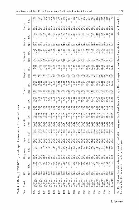
The orders p of the AR and q of the MA are determined using the SchwarzBayesian information criterion (SBC). The SBC is a statistic commonly used toselect between competing models.5 It takes into account the goodness-of-fit of eachmodel and it penalizes models in relation to the number of parameters. The modelchosen, i.e. the orders of p and q, is that for which the SBC is minimized. The SBCsare calculated for models with p and q up to five lags for each series to account for aweek of data. The orders of the models are re-defined every year to adapt theforecasts to the medium-term dynamics of the series (these are reported in Tables 3and 4). The short-term dynamics are captured by performing 1 day ahead out-of-sample forecasts resulting from the estimation of the model with the previous 60observations (i.e., data for approximately one quarter). The size of the rollingwindow is chosen in accordance with McGough and Tsolacos (1995) and Tse (1997)who suggest that the minimum number of observations needed for generating anARMA model is 50 observations. The sample is rolled forward by including a new

5 Akaike’s information criterion (AIC) is often also used to select between competing models, but as notedby Mills (1990), the AIC can result in the selection of an over-parametrized model.


Tab

le3

ARMA(p,q)–EGARCH(x,y)mod

elspecifications

used

toforecastsecuritized

real

estate

returns

Year

Model

U.S.

HongKong

Japan

Australia

U.K.

France

Singapore

Netherlands

Germany

Sweden

Spec

SBC

Spec

SBC

Spec

SBC

Spec

SBC

Spec

SBC

Spec

SBC

Spec

SBC

Spec

SBC

Spec

SBC

Spec

SBC

1992

ARMA

(0,1)

−7.04

(4,4)

−5.83

(0,1)

−5.42

(3,3)

−6.90

(4,4)

−6.54

(0,3)

−6.84

(5,5)

−5.75

(4,4)

−7.23

(3,0)

−6.96

(3,3)

−5.03

EGARCH

(5,5)

−15.63

(3,3)

−12.15

(3,3)

−12.70

(3,3)

−15.20

(5,5)

−13.11

(4,4)

−15.02

(1,0)

−11.12

(5,5)

−15.26

(1,1)

−13.61

(3,3)

−10.61

1993

ARMA

(0,1)

−7.72

(0,2)

−5.42

(4,1)

−4.99

(0,1)

−7.16

(5,1)

−5.63

(0,1)

−7.08

(1,0)

−6.04

(0,1)

−7.54

(0,1)

−6.78

(5,0)

−4.11

EGARCH

(3,3)

−16.96

(5,5)

−7.19

(1,0)

−10.18

(5,5)

8.23

(5,5)

−0.07

(2,2)

−15.74

(5,5)

13.58

(1,1)

−14.90

(1,1)

−11.60

(1,1)

16.89

1994

ARMA

(1,4)

−7.62

(2,0)

−5.48

(0,1)

−5.15

(0,4)

−7.02

(3,0)

−6.23

(2,2)

−7.59

(3,3)

−6.04

(1,0)

−7.60

(2,2)

−6.71

(1,5)

−4.35

EGARCH

(1,1)

−16.46

(5,5)

−11.45

(2,2)

−9.04

(3,3)

−15.54

(5,5)

1.03

(5,5)

−14.17

(1,1)

−11.12

(1,1)

−16.74

(2,2)

−13.40

(1,1)

−10.15

1995

ARMA

(1,0)

−7.91

(3,0)

−4.87

(4,4)

−5.84

(2,1)

−6.94

(5,5)

−6.37

(1,1)

−6.87

(4,4)

−5.30

(3,3)

−7.42

(0,1)

−6.61

(5,5)

−5.30

EGARCH

(5,5)

−14.35

(3,3)

−12.29

(2,2)

−10.48

(2,2)

−15.04

(5,5)

−13.60

(5,5)

11.79

(1,0)

−6.75

(5,5)

−16.54

(3,3)

−13.47

(5,5)

−11.46

1996

ARMA

(1,0)

−8.50

(5,5)

−5.79

(5,5)

−5.21

(4,0)

−7.30

(5,5)

−6.68

(5,0)

−7.06

(5,5)

−5.71

(0,4)

−7.79

(0,3)

−6.91

(4,4)

−5.97

EGARCH

(5,5)

−18.20

(2,2)

2.59

(1,0)

−8.89

(5,5)

−15.35

(1,1)

−13.40

(5,5)

−14.18

(2,0)

−10.65

(5,5)

7.56

(3,3)

−12.86

(4,4)

−11.91

1997

ARMA

(1,1)

−8.30

(0,2)

− 6.11

(3,3)

−5.84

(3,3)

−7.44

(2,0)

−7.26

(3,3)

−7.91

(5,5)

−5.62

(5,5)

−7.98

(3,0)

−4.96

(3,3)

−6.38

EGARCH

(1,0)

−16.62

(5,0)

−12.54

(2,1)

−9.64

(1,1)

−15.33

(5,5)

12.23

(3,1)

−15.01

(4,4)

−2.69

(2,2)

−14.51

(5,5)

−9.04

(3,3)

−11.70

1998

ARMA

(0,1)

−7.55

(3,3)

−4.77

(4,4)

−4.66

(4,0)

−6.66

(0,5)

−6.33

(4,4)

−7.10

(1,0)

−4.93

(5,5)

−7.07

(4,4)

−6.61

(0,4)

−6.32

EGARCH

(1,1)

−15.21

(3,3)

−6.97

(5,5)

−9.21

(5,5)

9.12

(5,0)

−14.28

(1,1)

21.40

(1,1)

7.27

(1,1)

−10.01

(4,4)

−12.72

(5,5)

12.01

1999

ARMA

(0,1)

−6.63

(5,5)

−3.84

(2,2)

−4.12

(4,4)

−6.58

(3,3)

−6.88

(2,2)

−7.09

(5,5)

−3.33

(5,0)

−7.40

(0,5)

−5.56

(4,4)

−6.53

EGARCH

(2,1)

−13.83

(1,0)

−7.97

(5,5)

14.68

(4,4)

−13.89

(1,1)

−13.37

(2,2)

− 12.95

(5,5)

−8.73

(1,1)

−7.95

(1,1)

−10.20

(3,3)

−13.76

2000

ARMA

(0,1)

−7.38

(4,4)

−5.11

(0,2)

−4.47

(0,4)

−6.78

(5,5)

−6.95

(4,4)

−7.15

(4,4)

−4.58

(4,4)

−7.24

(5,5)

−5.35

(4,4)

−7.30

EGARCH

(3,3)

−15.18

(5,5)

8.44

(2,2)

−9.04

(5,5)

−14.21

(5,5)

−13.19

(1,0)

−14.17

(5,5)

−9.95

(5,5)

−15.30

(4,0)

−11.49

(3,0)

−12.77

2001

ARMA

(4,4)

−7.07

(3,3)

−5.01

(2,2)

−4.78

(5,5)

−7.14

(1,0)

−7.06

(0,1)

−7.01

(2,2)

−4.79

(0,3)

−7.79

(4,4)

−5.61

(3,3)

−6.39

EGARCH

(2,1)

−15.34

(1,0)

−9.46

(2,2)

−10.53

(1,0)

−14.77

(3,3)

−14.13

(1,0)

−14.07

(5,5)

−8.99

(2,1)

−15.54

(1,1)

−0.78

(1,1)

9.12

2002

ARMA

(0,3)

−6.83

(3,3)

−5.06

(3,3)

−5.04

(5,5)

−6.89

(4,1)

−7.12

(2,2)

− 7.12

(5,5)

−4.59

(5,5)

−7.47

(4,4)

−5.55

(4,0)

−6.45

EGARCH

(1,1)

14.61

(5,5)

−11.07

(2,2)

−9.93

(4,0)

−14.24

(1,1)

−15.51

(1,0)

−15.19

(2,1)

−9.26

(1,0)

−16.44

(1,1)

21.93

(1,1)

−12.37

2003

ARMA

(4,2)

−6.48

(4,4)

−5.50

(5,5)

−4.88

(3,3)

−7.90

(5,5)

−6.62

(4,0)

−6.27

(5,5)

−5.30

(1,0)

−7.13

(0,3)

−4.65

(2,2)

−6.52

EGARCH

(1,1)

−12.89

(1,1)

−11.04

(5,5)

−10.38

(2,2)

−15.20

(2,0)

18.90

(1,1)

−11.83

(5,5)

−10.54

(2,2)

−13.21

(3,3)

−8.59

(3,3)

−14.54

2004

ARMA

(0,5)

−6.91

(3,1)

−5.28

(0,1)

−4.93

(0,1)

−7.29

(1,0)

−6.63

(1,1)

−7.22

(3,3)

−5.05

(5,5)

−7.44

(0,5)

−5.29

(4,4)

−7.16

EGARCH

(5,5)

−13.25

(2,1)

−9.07

(1,0)

−9.36

(5,5)

−14.74

(4,4)

−12.25

(1,0)

−15.59

(1,1)

− 10.05

(1,0)

−15.22

(4,4)

−11.93

(2,2)

−13.95

2005

ARMA

(4,4)

−6.21

(4,4)

−5.46

(2,2)

−5.42

(5,5)

−7.33

(0,5)

−7.22

(3,3)

−6.98

(5,5)

−6.60

(4,4)

−7.42

(4,4)

−7.47

(0,2)

−6.97

EGARCH

(5,5)

−12.33

(5,5)

−12.23

(5,5)

−12.68

(1,1)

−15.23

(5,5)

−15.50

(1,0)

−13.84

(3,1)

−11.58

(3,3)

−13.48

(3,3)

−13.05

(5,5)

−12.85

2006

ARMA

(3,3)

−6.42

(5,5)

−6.54

(5,5)

−5.95

(4,4)

−7.08

(0,4)

−6.90

(5,5)

−6.58

(5,5)

−6.48

(5,5)

−7.17

(3,0)

−6.58

(2,0)

−5.95

EGARCH

(1,0)

−12.92

(5,5)

−11.47

(1,1)

−9.98

(4,4)

−14.69

(2,2)

−12.63

(1,1)

−5.77

(5,5)

−9.72

(2,2)

−13.44

(2,1)

−12.01

(4,4)

−12.96

2007

ARMA

(0,1)

−6.56

(5,5)

−6.18

(5,5)

−5.36

(0,3)

−6.84

(5,5)

−5.93

(0,3)

−6.04

(0,1)

−5.88

(4,0)

−6.33

(2,2)

−5.77

(0,3)

−5.57

EGARCH

(5,5)

1.50

(5,5)

7.71

(2,2)

−11.31

(2,0)

−12.40

(1,0)

−12.38

(3,0)

−11.64

(5,5)

−0.99

(5,5)

−3.87

(1,1)

3.20

(2,2)

−12.47

The

SBC(SchwarzBayesianinform

ationcriterion)iscalculated

everyyear

forallm

odelsup

tofive

lags.T

histablereportsthemodelsused

tomaketheforecasts,i.e.the

models

forwhich

theSBCisminim

ized

intheprevious

year


Tab

le4

ARMA(p,q)−EGARCH(x,y)model

specifications

used

toforecaststockreturns

Year

Model

U.S.

HongKong

Japan

Australia

U.K.

France

Singapore

Netherlands

Germany

Sweden

Spec

SBC

Spec

SBC

Spec

SBC

Spec

SBC

Spec

SBC

Spec

SBC

Spec

SBC

Spec

SBC

Spec

SBC

Spec

SBC

1992

ARMA

(3,3)

−6.68

(3,0)

−6.17

(5,5)

−6.25

(2,0)

−6.51

(5,5)

−6.94

(5,5)

−6.35

(5,5)

−6.55

(3,3)

−7.28

(3,0)

−6.33

(5,5)

−5.85

EGARCH

(4,4)

−14.84

(4,4)

−10.99

(3,3)

−12.77

(1,1)

−13.69

(4,3)

−14.52

(5,5)

10.98

(2,2)

−7.27

(1,1)

−14.47

(5,5)

−11.61

(4,4)

−12.52

1993

ARMA

(2,2)

−7.43

(0,3)

−5.74

(0,1)

−5.62

(0,1)

−7.02

(0,1)

−6.52

(4,0)

−6.41

(0,5)

−7.07

(4,4)

−7.56

(3,3)

−7.17

(0,1)

−5.26

EGARCH

(1,0)

−13.53

(3,3)

−13.01

(5,3)

−10.57

(2,0)

−15.98

(5,5)

0.31

(1,1)

−10.84

(1,1)

−13.69

(3,3)

−15.15

(5,5)

−15.07

(2,2)

−9.92

1994

ARMA

(2,2)

−7.63

(1,0)

−5.79

(0,1)

−6.07

(0,1)

−7.00

(4,4)

−7.54

(5,5)

−6.86

(1,0)

−7.33

(1,0)

−7.64

(0,1)

−7.19

(0,1)

−6.32

EGARCH

(4,4)

−15.14

(1,1)

−12.07

(5,5)

−12.79

(5,5)

−15.65

(1,1)

4.25

(1,1)

−14.58

(1,1)

−14.09

(5,5)

−14.95

(3,3)

−14.35

(4,4)

−14.36

1995

ARMA

(5,0)

−7.39

(4,4)

−5.27

(3,3)

−6.75

(5,5)

−6.61

(3,3)

−6.95

(5,5)

−6.60

(4,4)

−6.36

(4,4)

−7.19

(0,5)

−6.82

(5,5)

−6.32

EGARCH

(1,0)

−15.62

(1,1)

−11.12

(1,1)

−13.46

(2,2)

−15.09

(1,1)

−5.86

(4,4)

−13.46

(5,5)

−13.75

(5,5)

−15.79

(1,1)

−15.75

(3,0)

−9.50

1996

ARMA

(5,0)

−7.79

(5,5)

−6.07

(4,4)

−6.18

(0,1)

−7.17

(5,5)

−7.60

(0,5)

−6.65

(0,1)

−6.84

(3,3)

−7.75

(0,5)

−7.31

(0,5)

−6.60

EGARCH

(4,4)

−16.39

(2,2)

−5.27

(5,5)

−12.59

(5,0)

−13.86

(1,0)

−14.71

(4,4)

−13.14

(1,1)

7.27

(5,5)

−13.74

(3,3)

−15.87

(3,1)

−12.44

1997

ARMA

(1,0)

−7.03

(0,2)

−6.38

(5,5)

−7.06

(5,5)

−6.96

(0,5)

−7.67

(5,5)

−7.21

(5,5)

−6.82

(0,4)

−7.17

(0,1)

−7.24

(3,3)

−6.79

EGARCH

(2,0)

−16.12

(5,5)

−13.73

(1,1)

−13.36

(1,1)

−14.58

(5,5)

−15.57

(1,1)

−14.43

(5,0)

−10.42

(4,4)

−12.29

(3,1)

−15.19

(5,5)

−13.95

1998

ARMA

(0,2)

−6.23

(3,3)

−4.75

(2,0)

−5.83

(3,3

−6.37

(3,3)

−6.76

(4,4)

−6.02

(0,4)

−5.90

(4,0)

−5.78

(4,0)

−5.94

(0,4)

−5.92

EGARCH

(1,0)

−13.49

(1,1)

−8.95

(5,5)

−11.89

(5,5)

13.03

(1,1)

−14.31

(1,1)

13.28

(4,4)

−10.47

(1,1)

−13.05

(2,1)

−13.19

(5,5)

−6.54

1999

ARMA

(5,5)

−5.93

(5,5)

−4.46

(5,0)

−5.81

(0,1)

−6.35

(0,1)

−6.05

(0,1)

−5.63

(5,5)

−4.99

(0,1)

−5.46

(2,0)

−5.51

(4,4)

−5.21

EGARCH

(4,4)

−12.73

(2,2)

−9.01

(1,1)

−13.42

(1,1)

−12.14

(5,5)

−11.64

(1,1)

−10.31

(1,1)

−10.95

(1,1)

−12.92

(1,1)

−12.87

(1,1)

−11.47

2000

ARMA

(4,4)

−6.16

(4,4)

−5.48

(0,3)

−6.07

(0,4)

−6.76

(4,4)

−6.44

(4,4)

−6.30

(4,4)

−5.70

(4,4)

−6.26

(1,1)

−6.05

(4,4)

−6.00

EGARCH

(1,1)

−12.59

(4,1)

−10.15

(4,4)

−13.28

(2,2)

−15.39

(3,3)

−12.28

(3,3)

−9.72

(5,5)

14.64

(1,1)

−10.93

(4,1)

−13.51

(1,1)

−11.29

2001

ARMA

(4,4)

−7.07

(3,3)

−5.01

(2,2)

−4.78

(5,5)

−7.14

(1,0)

−7.06

(0,1)

−7.01

(2,2)

−4.79

(0,3)

−7.79

(4,4)

−5.61

(3,3)

−6.39

EGARCH

(2,1)

−9.56

(2,1)

−9.49

(1,0)

−11.80

(1,0)

−13.09

(2,1)

−11.66

(5,5)

−11.22

(5,5)

−9.77

(5,5)

−13.44

(5,3)

−12.23

(5,5)

−5.97

2002

ARMA

(5,5)

−5.76

(3,3)

−5.41

(4,0)

−5.58

(3,3)

−6.81

(2,2)

−5.94

(4,4)

−5.56

(3,0)

−5.84

(2,2)

−5.63

(4,4)

−5.53

(5,5)

−4.90

EGARCH

(5,5)

2.52

(1,1)

−10.96

(1,0)

−10.63

(1,1)

−13.37

(1,1)

−13.79

(1,0)

−11.90

(2,2)

19.57

(1,1)

−12.45

(5,5)

3.14

(5,5)

−9.17

2003

ARMA

(0,4)

−5.44

(4,4)

−6.14

(5,5)

−5.77

(0,4)

−7.08

(0,3)

−5.50

(3,3)

−5.07

(5,5)

−6.22

(3,3)

−5.02

(5,5)

−5.31

(5,5)

−4.99

EGARCH

(5,5)

13.74

(5,5)

0.62

(5,2)

−13.88

(2,1)

−14.02

(1,1)

−10.59

(5,5)

−10.25

(1,1)

−12.73

(1,1)

−8.78

(2,0)

−10.78

(1,1)

−9.53

2004

ARMA

(5,5)

−6.33

(0,3)

−6.32

(4,4)

−6.00

(5,5)

−7.35

(5,5)

−6.21

(5,5)

−5.72

(0,1)

−6.25

(5,5)

−5.55

(4,4)

−5.75

(5,5)

−5.93

EGARCH

(4,4)

− 14.78

(5,0)

−11.51

(4,4)

−11.83

(1,1)

−15.36

(5,5)

−14.69

(4,4)

−11.97

(4,4)

−12.11

(5,5)

−8.47

(4,4)

−12.59

(5,5)

−12.52

2005

ARMA

(1,1)

−7.13

(5,5)

−6.33

(4,4)

−6.34

(3,3)

−8.14

(0,2)

−7.37

(5,5)

−6.89

(4,4)

−7.12

(5,5)

−6.90

(5,5)

−6.88

(2,0)

−6.48

EGARCH

(3,1)

−13.07

(5,5)

−14.17

(1,1)

−3.80

(1,1)

−15.75

(1,1)

−14.30

(3,3)

−13.21

(2,0)

−15.71

(5,5)

−13.43

(5,5)

−14.10

(5,5)

−13.69

2006

ARMA

(3,3)

−7.29

(5,5)

−7.19

(5,5)

−6.86

(4,4)

−7.37

(4,0)

−7.62

(3,3)

−7.32

(4,4)

−7.45

(5,5)

−7.39

(3,0)

−7.47

(2,2)

−7.04

EGARCH

(3,3)

−15.28

(1,1)

−13.09

(5,5)

0.24

(3,3)

−14.16

(3,0)

−16.79

(4,4)

−14.15

(5,5)

−0.20

(4,4)

15.57

(5,5)

1.66

(1,1)

−14.68

2007

ARMA

(2,0)

−7.29

(4,4)

−6.64

(3,3)

−6.09

(0,1)

−6.81

(3,0)

−6.85

(3,3)

−6.67

(5,0)

−6.79

(0,3)

−6.71

(3,3)

−6.74

(3,0)

−6.05

EGARCH

(1,0)

−13.33

(5,0)

−12.37

(5,5)

6.96

(3,1)

−13.29

(5,0)

−15.28

(2,2)

−12.59

(5,5)

12.17

(1,1)

−13.08

(5,5)

−14.06

(1,0)

−11.92

The

SBC(SchwarzBayesianinform

ationcriterion

)iscalculated

everyyear

forallm

odelsup

tofive

lags.T

histablerepo

rtsthemod

elsused

tomaketheforecasts,i.e.the

mod

els

forwhich

theSBCisminim

ized

intheprevious

year


observation and dropping the last one. Parameters are re-estimated at each step andnew forecasts are produced until the sample is exhausted.

ARMA–EGARCH Models

Financial markets are characterized by having periods that are more volatile thanothers. ARMA processes cannot model this fact as they assume a constant variance,but autoregressive conditional heteroscedastic (ARCH) processes can do so as theycapture time-varying but persistent volatility (Engle 1982). In ARCH models, thevariance of the error term hi,t is a function of the variances of the previous timeperiods’ error terms. An ARCH model may be described as follows:

ui;t ¼ffiffiffiffiffiffihi;t

pvt; ð2Þ

where hi;t ¼ V ui;t��ui;t�1; . . . ; ui;t�x

� � ¼ cþPxl¼1

ai;lu2i;t�l, ai,l represents the ARCHcoefficients, and vt � N 0; 1ð Þ.

The generalized autoregressive conditional heteroscedastic (GARCH) modelsconstitute a generalization of the ARCH models in which the variance of the errorterm is assumed to follow an ARMA process (Bollerslev 1986). Therefore, theautoregressive components are chosen in accordance with the ARMA analysis in theprevious section. A GARCH model may be described as follows:


pvt; ð3Þ

where hi;t ¼ V ui;t ui;t�1; . . . ; ui;t�x

�� ¼ cþPxl¼1

ai;lu2i;t�l þPym¼1

bi;mhi;t�m, bi,m represents

the GARCH coefficients, c, ai,l, and bi,m are positive to ensure that the conditionalvariance is positive, and vt � N 0; 1ð Þ.

Even though numerous variations and extensions of these models have beendeveloped, the only extension we will consider is the exponential generalizedautoregressive conditional heteroscedastic (EGARCH) models (Nelson 1991). Thebenefits of EGARCH models have been pointed out by Pagan and Schwert (1990),Hentschel (1995), and Brandt and Jones (2006).6 EGARCH models capture the mostimportant stylized features of stock return volatility, i.e. time series clustering,negative correlation with returns, lognormality, and with certain specifications, longmemory (Andersen et al. 2001). The logarithmic transformation of this specificationguarantees that the conditional variance will be positive without having to imposeany constraints on the coefficients. Other extensions (TARCH, SWARCH,QTARCH, etc.) could provide better forecasts, but with additional assumptions ourapproach could loose the ‘neutrality’ that we are looking for. An EGARCH modelmay be described as follows:


pvt; ð4Þ

6 For a review of the volatility forecasting literature, see Poon and Granger (2003). They summarize themethodologies and empirical findings of 93 papers that study the forecasting performance of variousvolatility models and find that the choice of a model is to some extent data and period specific.


where ln hi;t� � ¼ cþPx

l¼1ai;lg vt�lð Þ þ Py

m¼1bi;m ln hi;t�m

� �, g vtð Þ ¼ qvt þ l vtj j�½ E vtj j�,

and vt � N 0; 1ð Þ.The model estimated in this paper is an ARMA–EGARCH model so that we can

forecast the level of the series, ri,t, as well as its variance. The ARMA–EGARCHmodel is simply an ARMA model where the residual term, ui,t, is assumed to beGaussian white noise with variance denoted by the EGARCH model. The ARMA–EGARCH model used is:

ri;t ¼ mþXpj¼1

fi;jri;t�j �Xqk¼0

qi;kui;t�k ð5Þ

where ui;t � N 0; hi;t� �

.Table 3 reports the chosen ARMA and ARMA–EGARCH models for each year

and country for securitized real estate, while Table 4 does the same for stocks. Asexpected, the model specifications and parameter estimates (not reported) for bothasset classes vary somewhat over time in all the countries.7 This highlights the needof using a dynamic method in which we adapt the models (at a yearly frequency) andthe parameter estimates (at a daily frequency) as new observations are madeavailable.

Predictability Comparisons

Prediction Errors and Excess Returns

The comparison of the predictability of securitized real estate and stocks, but also thecross-country comparisons, are undertaken by examining the entire empiricaldistributions of prediction errors (PEs). First, a graphical comparison is depicted byestimating the probability density functions (PDFs) of the PEs with a kernel-smoothingmethod. The kernel density estimate of series ri,t at point xi is estimated by:

bfi xið Þ ¼ 1

Th

XTt¼1

Kri;t � xi

h

� ð6Þ

where K ri;t�xih

� � ¼ 1ffiffiffiffi2p

p e�12

ri;t�xihð Þ2

is the Gaussian kernel, T is the number ofobservations, and h is the smoothing parameter or bandwidth, estimated with thefollowing rule of thumb h ¼ bsT�1= 5. Then, the Kruskal-Wallis test is employed todetermine if the differences between the empirical distributions of the PEs aresignificant.

The Kruskal-Wallis test is a straightforward generalization of the Wilcoxon Rank-Sum or Mann-Whitney test where K independent samples can be tested. TheWilcoxon test is a non-parametric test for determining whether two independentsamples come from the same distribution. The null hypothesis tested is that the twosamples are drawn from a single population, and therefore that their probabilitydistributions are equal. This test is based on the idea that the sum of the ranks for the

7 Since we do not perform our forecasts with a single, static model, but with a model that evolves andadapts itself through time, we do not use other diagnostic tests as we are already using the SBC criterion tochoose the most appropriate specification.


samples above and below the median should be similar. In the Kruskal-Wallis test,the K independent samples of sizes n1,…,nK are all combined into one large sample,they are sorted from smallest to largest and ranks are assigned (assigning the averagerank to any observation in a group of tied observations). Then, the average of theranks of the observations in the i-th sample, Ri, is obtained and the test statistic iscalculated as follows:

KW ¼ 12

N N þ 1ð ÞXKi¼1

ni Ri � N þ 1

2

�2

ð7Þ

where the null hypothesis that all K distributions are the same is rejected ifKW > #2K�1. Since we believe that forecasting performance should not focus on theforecasts per se, but on the outcomes of the investment decisions taken with thoseforecasts, the same procedure is repeated, but instead of using PEs, we use theexcess returns of an active trading strategy (to be described below) over a buy-and-hold investment.

Trading Strategies

To evaluate the performance of the predictions both across asset classes and acrosscountries, we use the forecasts to construct active trading strategies and benchmarkthem against a buy-and-hold strategy. Under the assumption that an investor takes along position either on real estate securities or on the risk free asset, the followingtrading rules are applied. If securitized real estate return forecasts are higher than therisk free asset’s mean return for the previous 60 days, the investor will go long onreal estate securities; otherwise the investor will go long the risk free asset. The sameprocedure is employed for stocks. At this point, no transaction costs are taken intoaccount, but we also calculate the round-trip transaction costs that would equate theactive strategy to the passive one. Note that benchmarking with a buy-and-holdinvestment entails that the active strategy will outperform the passive strategy ifmarket downturns can be accurately predicted in a bull market whereas in a bearmarket, a passive strategy can be outperformed by being long the risk free asset and/or by accurately predicting market upturns; when short selling is not allowed.Therefore, outperforming a buy-and-hold investment is more difficult in bull marketsthan in bear markets.

Predictability Results

Comparisons based on Prediction Errors and Excess Returns

The predictability of securitized real estate and stock returns is first compared ineach country with the PDFs of the prediction errors obtained with ARMA andARMA–EGARCH forecasts. Such comparisons are illustrated in Figs. 1 and 2,respectively. Both figures show that securitized real estate PDFs dominate stockPDFs in the U.S. and the Netherlands. Inversely, both figures also show that stockPDFs dominate securitized real estate PDFs in Japan, Australia, the U.K., Singapore,


Germany, and Sweden. In Hong Kong and France, the results depend on theforecasting technique used.

The differences between two PDFs might be difficult to establish graphically insome cases, so the Kruskal-Wallis test is used to determine if the differences betweeneach pair of empirical distributions are significant (second column of Table 5).8

Based on the ARMA forecasts, securitized real estate returns appear morepredictable than stock returns in the Netherlands (at the 1% level), whereas stockreturns appear more predictable than securitized real estate returns in Japan, theUnited Kingdom, and Germany (at the 1% level). Based on the ARMA–EGARCHforecasts, securitized real estate returns appear more predictable than stock returns inFrance (at the 10% level). The opposite conclusion holds for Sweden (at the 5%level). For the remainder of countries, both asset classes appear to be equallypredictable. For the U.S., our results thus differ from the findings of Liu and Mei(1992) and Liao and Mei (1998), but are consistent with those of Mei and Lee

-0.04 -0.02 0 0.02 0.040

0.05United States

PEs

PD

Fs

Securitized Real EstateStocks

-0.04 -0.02 0 0.02 0.040

0.05Hong Kong

PEs

PD

Fs

-0.04 -0.02 0 0.02 0.040

0.05Japan

PEs

PD

Fs

-0.04 -0.02 0 0.02 0.040

0.05Australia

PEs

PD

Fs

-0.04 -0.02 0 0.02 0.040

0.05United Kingdom

PEs

PD

Fs

-0.04 -0.02 0 0.02 0.040

0.05France

PEs

PD

Fs

-0.04 -0.02 0 0.02 0.040

0.05Singapore

PEs

PD

Fs

-0.04 -0.02 0 0.02 0.040

0.05Netherlands

PEs

PD

Fs

-0.04 -0.02 0 0.02 0.040

0.05Germany

PEs

PD

Fs

-0.04 -0.02 0 0.02 0.040

0.05Sweden

PEs

PD

Fs

Fig. 1 Probability density functions of the ARMA prediction errors

8 Table 5 makes it possible to assess the significance of differences, but the determination of which assetclass is more predictable is based on graphical inspection of the distributions (Figs. 1 and 2).


Table 5 P-values of the Kruskal-Wallis test

Country Prediction errors Excess returns

ARMA ARMA–EGARCH ARMA ARMA–EGARCH

U.S. 0.25 0.69 0.12 0.07a

Hong Kong 0.20 0.54 0.04b 0.04b

Japan 0.00c 0.99 0.16 0.03b

Australia 0.95 0.90 0.97 0.88U.K. 0.00c 0.32 0.17 0.27France 0.87 0.09a 0.28 0.02b

Singapore 0.97 0.38 0.03b 0.01c

Netherlands 0.01c 0.77 0.01c 0.01c

Germany 0.00c 0.37 0.00c 0.01c

Sweden 0.48 0.04b 0.56 0.11

The null hypothesis tested is that the probability distributions of both asset classes are equala Rejection of the null hypothesis at the 10% levelb Rejection of the null hypothesis at the 5% levelc Rejection of the null hypothesis at the 1% level

-0.04 -0.02 0 0.02 0.040

0.05United States

PEs

PD

Fs

-0.04 -0.02 0 0.02 0.040

0.05Hong Kong

PEs

PD

Fs

-0.04 -0.02 0 0.02 0.040

0.05Japan

PEs

PD

Fs

-0.04 -0.02 0 0.02 0.040

0.05Australia

PEs

PD

Fs

-0.04 -0.02 0 0.02 0.040

0.05United Kingdom

PEs

PD

Fs

-0.04 -0.02 0 0.02 0.040

0.05France

PEs

PD

Fs

-0.04 -0.02 0 0.02 0.040

0.05Singapore

PEs

PD

Fs

-0.04 -0.02 0 0.02 0.040

0.05Netherlands

PEs

PD

Fs

-0.04 -0.02 0 0.02 0.040

0.05Germany

PEs

PD

Fs

-0.04 -0.02 0 0.02 0.040

0.05Sweden

PEs

PD

Fs


Fig. 2 Probability density functions of the ARMA–EGARCH prediction errors


(1994) and Li and Wang (1995), even if the framework used in these studies mightbias their conclusions in this regard.

From an investment point of view, the accuracy of a forecast is not as importantas the outcome of the investment decision made with the forecast. Therefore, thepredictability of the two asset classes in each country is compared in a morepragmatic manner by replacing the prediction errors in the analysis by the excessreturns of the active trading strategy over the buy-and-hold investment. Using excessreturns enriches the analysis as the results show if the differences in predictability areeconomically significant. The last column of Table 5 contains the results of theKruskal-Wallis test for differences in the distributions of excess returns. Only thesignificantly different PDFs of ARMA and ARMA–EGARCH excess returns arepresented in Fig. 3. Overall, the results show that the predictability of securitized realestate and stock returns differs in some countries. Securitized real estate appears tobe more predictable in the Netherlands with the two forecasting techniques, and in

-4 -2 0 2 4

x 10-3

00.20.4

ARMA - Hong Kong

Excess Returns

PD

Fs


-4 -2 0 2 4

x 10-3

00.20.4

ARMA - Singapore

Excess Returns

PD

Fs

-4 -2 0 2 4

x 10-3

00.20.4

ARMA - Netherlands

Excess Returns

PD

Fs

-4 -2 0 2 4

x 10-3

00.20.4

ARMA - Germany

Excess Returns

PD

Fs

-4 -2 0 2 4

x 10-3

00.20.4

ARMA-EGARCH - United States

Excess Returns

PD

Fs

-4 -2 0 2 4

x 10-3

00.20.4

ARMA-EGARCH - Hong Kong

Excess Returns

PD

Fs

-4 -2 0 2 4

x 10-3

00.20.4

ARMA-EGARCH - Japan

Excess Returns

PD

Fs

-4 -2 0 2 4

x 10-3

00.20.4

ARMA-EGARCH - France

Excess Returns

PD

Fs

-4 -2 0 2 4

x 10-3

00.20.4

ARMA-EGARCH - Singapore

Excess Returns

PD

Fs

-4 -2 0 2 4

x 10-3

00.20.4

ARMA-EGARCH - Netherlands

Excess Returns

PD

Fs

-4 -2 0 2 4

x 10-3

00.20.4

ARMA-EGARCH - Germany

Excess Returns

PD

Fs

Fig. 3 Significantly different probability density functions of ARMA and ARMA–EGARCH excess returns


the U.S. and France with the ARMA–EGARCH models.9 Stocks appear to be morepredictable with the two forecasting techniques in Hong Kong, Singapore, andGermany, and with the ARMA–EGARCH models in Japan.

Hence, some differences exist between the results obtained with prediction errorsand excess returns of an active strategy over a buy-and-hold investment. In line withGerlow et al. (1993), our results show that statistical criteria may be misleading fordetermining the potential profitability of a forecast in a trading strategy. However, acommon result that emerges from the different methodologies is that securitized realestate returns are generally more predictable than stock returns in countries with wellestablished REIT regimes. Securitized real estate returns are indeed more predictablethan stock returns in the U.S. and the Netherlands, countries where REIT regimesexist since 1960 and 1969, respectively. On the other hand, stock returns are morepredictable than securitized real estate returns in some of the countries that have onlyestablished REIT regimes in the recent past.

The greater predictability of securitized real estate returns in mature REIT marketsis intuitively appealing as such vehicles have more stable income returns (cashflows) as their investment focus is on income producing real estate and are requiredto distribute at least 90% of their income as dividends to qualify for tax transparencyin the U.S. (100% in the Netherlands). Related to this issue, Pagliari et al. (2005)show that there is no difference from a statistical point of view between REIT anddirect real estate returns in the U.S. once REIT returns have been deleveraged, directreal estate returns desmoothed, and portfolio composition effects corrected for.Evidence thus emerges for tax transparent real estate vehicles to behave more likedirect investments, in particular with respect to a regular income stream.

It is further worthwhile to perform some cross-country comparisons; these pertainto securitized real estate only. The predictability of ARMA models across countriesis assessed in Fig. 4, Panel A. The properties displayed by the PDFs of the predictionerrors show that differences in predictability exist across countries. The bestforecasts using ARMA models are obtained in the Netherlands, the U.S., andAustralia. According to the Kruskal-Wallis test (not reported for the cross-countrycomparisons), the top three countries have empirical distributions which aresignificantly different from those of the other countries at the 5% level. The resultsregarding the ARMA–EGARCH forecasts (Fig. 4, Panel B) are similar to those ofthe ARMA forecasts, but lack statistical significance.

Figure 5 displays securitized real estate’s empirical distributions across countriesusing excess returns instead of prediction errors. Since excess returns evaluate thedecisions made with the forecasts, whereas prediction errors evaluate the accuracy ofthe forecasts, it is not surprising that the PDFs of the former are steeper than those ofthe latter (note that the x-axes have different units). Indeed, with the trading strategy,there will only be an ‘error’ when the decision being made is to go long the risk freeinvestment as else the two strategies will be identical. Both time series techniquesreveal similar results. The Kruskal-Wallis tests identify two groups of countries withdifferent predictability patterns. Australia, the Netherlands, the U.S., France, theU.K., Germany, and Sweden belong to the group with higher predictability, while

9 The ARMA results are consistent with Nelling and Gyourko’s (1998) findings for the United States astheir AR models reveal that EREITs and mid caps are equally predictable.


Singapore, Hong Kong, and Japan are in the one with lower predictability. Thecontrasting results for Asia are not surprising as a different continental environmentand performance behavior have been documented (Ooi and Liow 2004; Hoesli andSerrano 2007). In sum, the results obtained with the cross-country comparisonsconfirm those obtained with the across asset comparisons; the predictability of

-5 -4 -3 -2 -1 0 1 2 3 4 5x 10 -3

0

0.05

0.1

0.15

0.2

0.25

0.3

0.35

0.4Panel A - ARMA

Excess Returns

Pro

babi

lity

Den

sity

Fun

ctio

ns

-5 -4 -3 -2 -1 0 1 2 3 4 5x 10-3

0

0.05

0.1

0.15

0.2

0.25

0.3

0.35

0.4Panel B - ARMA-EGARCH

Excess Returns

Pro

babi

lity

Den

sity

Fun

ctio

ns

United StatesHong KongJapanAustraliaUnited KingdomFranceSingaporeNetherlandsGermanySweden


Fig. 5 Securitized real estate’s probability density functions of the excess returns

-0.05 -0.04 -0.03 -0.02 -0.01 0 0.01 0.02 0.03 0.04 0.050

0.01

0.02

0.03

0.04

0.05Panel A - ARMA

Prediction Errors

Pro

babi

lity

Den

sity

Fun

ctio

ns

-0.05 -0.04 -0.03 -0.02 -0.01 0 0.01 0.02 0.03 0.04 0.050

0.01

0.02

0.03

0.04

0.05Panel B - ARMA-EGARCH

Prediction Errors

Pro

babi

lity

Den

sity

Fun

ctio

ns



Fig. 4 Securitized real estate’s probability density functions of the prediction errors


securitized real estate returns is greater in the countries with the more establishedREIT regimes (i.e. the U.S., the Netherlands, and Australia).

Trading Strategy Comparisons

The results of the trading strategies using the ARMA and ARMA–EGARCHforecasts without taking transaction costs into account are shown in Table 6. Forcomparison purposes, we also report the results of buy-and-hold strategies. Theinitial wealth in each case is 1,000 units of local currency. A buy-and-holdinvestment on securitized real estate outperforms a buy-and-hold investment onstocks in the U.S., Japan, Australia, and France. On the other hand, a buy-and-holdinvestment on stocks outperforms a buy-and-hold investment on securitized realestate in Hong Kong, the U.K., Singapore, the Netherlands, Germany, and Sweden.These results obviously highlight the varying average returns on the asset classes.The two active trading strategies outperform the buy-and-hold benchmark in allcountries for both asset classes. With the exception of Germany for securitized realestate and of France for stocks, the ARMA–EGARCH forecasts outperform theARMA forecasts in all the countries for the two asset classes. This results from thefact that the ARMA–EGARCH model is more complete as it takes into accountthe variance of returns in addition to mean returns. Overall, the trading strategieswork very well, but gains need to be put into perspective with the costs associatedwith such strategies.

Table 7 displays the transaction costs that would render the active strategyequivalent to a passive one. Such a focus is interesting as institutional and privateinvestors will have different transaction costs and can thus assess the usefulness ofthe reported strategies. These figures show that the active trading strategies generallyproduce better results for real estate securities than for stocks. In fact, the activetrading strategies allow for higher transaction costs for securitized real estate than forstocks in seven out of ten countries when ARMA models are used and in eight out of

Table 6 Terminal wealth for trading strategies vs buy-and-hold policies (January 1992–December 2007)

Country Securitized real estate Stocks

Trading strategy Buy-and-holdpolicy

Trading strategy Buy-and-holdpolicy

ARMA ARMA–EGARCH

ARMA ARMA–EGARCH

U.S. 19,940 26,614 9,606 11,363 14,787 5,237Hong Kong 40,093 109,838 7,567 41,614 96,646 10,896Japan 7,448 25,012 2,029 6,868 8,401 1,131Australia 12,423 14,518 8,617 11,832 15,191 7,429U.K. 17,238 17,873 4,779 14,988 19,912 5,154France 9,347 17,532 9,213 7,820 6,645 6,515Singapore 24,754 26,100 3,046 11,810 11,945 3,515Netherlands 13,963 14,491 4,852 19,114 23,753 6,986Germany 14,814 12,257 1,740 23,529 36,510 4,955Sweden 32,606 49,623 4,378 24,893 30,769 10,667

The initial investment is 1,000 units in local currency. No transaction costs are considered


ten countries when ARMA–EGARCH models are used; the ARMA–EGARCHmodels generally outperforming the ARMA models.

To determine if profits may be made with the forecasts, a possible benchmark touse is round-trip transaction costs amounting to 30 basis points (Chan andLakonishok 1993; Aitken and Frino 1996). With such a benchmark, the buy-and-hold investment is outperformed by active strategies net of transaction costs withboth forecasting techniques in Singapore, Germany, and Sweden for securitized realestate. Additionally, active strategies based on ARMA–EGARCH models outper-form the passive strategy in the presence of transaction costs in Hong Kong andJapan for securitized real estate and in Hong Kong, Japan, and Germany for stocks.Thus, active trading strategies outperform the buy-and-hold benchmark in fivecountries for real estate securities and in three for stocks, reinforcing the conclusionthat securitized real estate is generally more predictable than stocks.

Since the trading strategy is based on the time series forecasts, our approach isakin to that employed in studies of serial persistence. Therefore, our results supportthe good results of momentum strategies as reported by Cooper et al. (1999) and byStevenson (2002), whereas they contrast the findings of Mei and Gao (1995).Overall, the results indicate that time series forecasts help achieve higher profits thanthose obtained with a buy-and-hold investment once transaction costs are accountedfor in a number of countries.

Concluding Remarks

Although previous research has compared the predictability between securitized realestate and stock returns, the use of a multifactor asset pricing framework has resultedin potentially spurious conclusions due to the possible specification biasesintroduced in such comparisons. The time series approach followed in this papercreates a level playing field that allows to truly compare the predictability of returnsbetween the two asset classes. Therefore, our methodology provides the answers to aquestion that has been somewhat wrongfully addressed in the literature.

Table 7 Transaction costs rendering trading profits equal to buy-and-hold profits

Country Round-trip transaction costs (basis points)

Securitized real estate Stocks

ARMA ARMA–EGARCH ARMA ARMA–EGARCH

U.S. 18 23 12 16Hong Kong 25 43 23 38Japan 22 39 26 30Australia 6 9 9 14U.K. 21 23 19 22France 0 12 3 0Singapore 33 33 20 22Netherlands 18 20 16 20Germany 40 37 26 35Sweden 33 39 14 17


Empirical distributions of the prediction errors reveal differences in predictabilitybetween securitized real estate and stock returns. So is the case when excess returnsof an active strategy over a passive investment are used in the analysis. The latterresults, however, allow for the economic significance of the results to be assessed.These analyses show that the maturity of the securitized real estate market plays animportant role in the predictability of its returns. In particular, we find that incountries with established REIT regimes, securitized real estate returns are morepredictable than stock returns as the rental focus of REITs generates morepredictable income returns. Stated differently, tax transparency is likely to lead realestate securities to behave more like the underlying real estate assets. This finding isconfirmed with the cross-country comparisons of securitized real estate returnpredictability. Hence, the best forecasting accuracy is found in the U.S., theNetherlands, and to a lesser extent Australia; the countries with the three oldestREIT regimes in our sample.

Active trading strategies based on ARMA and especially on ARMA–EGARCHforecasts outperform the buy-and-hold benchmark in all the countries for both assetclasses. When transaction costs are taken into account, this remains the case in halfof our countries for real estate securities, but only in three for stocks. Given thatARMA–EGARCH models forecast the variance of returns in addition to meanreturns, they are generally more effective in devising investment strategies.

Further research could aim to find models and forecasting variables that lead toeconomically significant outcomes. The use of more complex active tradingstrategies could also contribute to this objective. Nonlinear models are also worthexploring, as well as using forecasting variables related to the well documentedhybrid nature of securitized real estate, i.e. the fact that real estate stocks encompassstock, bond, and real estate dimensions. A multivariate framework could beemployed to compare the predictability of securitized real estate and stock returnsprovided that an appropriate model driving the returns of each asset class could bedevised. Finally, future research could aim to further explain the factors that makeREITs more predictable than non-REITs.

Acknowledgements We are grateful to the participants of the AREUEA 2008 meetings in New Orleans,the European Real Estate Society 2008 conference in Krakow (Poland), and the 2008 Real Estate ResearchSymposium in Rotterdam (the Netherlands). An anonymous reviewer provided helpful comments. Theusual disclaimer applies.

References

Aitken, M., & Frino, A. (1996). Execution costs associated with institutional trades on the Australian stockexchange. Pacific Basin Finance Journal, 4(1), 45–58. doi:10.1016/0927-538X(95)00021-C.

Andersen, T. G., Bollerslev, T., Diebold, F. X., & Ebens, H. (2001). The distribution of realized stock returnvolatility. Journal of Financial Economics, 61(1), 43–76. doi:10.1016/S0304-405X(01)00055-1.

Bollerslev, T. (1986). Generalized autoregressive conditional heteroskedasticity. Journal of Econometrics,31(3), 307–327. doi:10.1016/0304-4076(86)90063-1.

Box, G. E. P., & Jenkins, G. M. (1976). Time Series Analysis: Forecasting and Control. San Francisco,CA: Holden-Day.

Brandt, M. W., & Jones, C. S. (2006). Volatility forecasting with range-based EGARCH models. Journalof Business & Economic Statistics, 24(4), 470–486. doi:10.1198/073500106000000206.


dx.doi.org/10.1016/0927-538X(95)00021-C

dx.doi.org/10.1016/S0304-405X(01)00055-1

dx.doi.org/10.1016/0304-4076(86)90063-1

dx.doi.org/10.1198/073500106000000206

Brooks, C., & Tsolacos, S. (2001). Forecasting real estate returns using financial spreads. Journal ofProperty Research, 18(3), 235–248. doi:10.1080/09599910110060037.

Brooks, C., & Tsolacos, S. (2003). International evidence on the predictability of returns to securitized realestate assets: Econometric models versus neural networks. Journal of Property Research, 20(2), 133–155. doi:10.1080/0959991032000109517.

Brown, J. P., Song, H., & McGillivray, A. (1997). Forecasting UK house prices: A time varyingcoefficient approach. Economic Modelling, 14(4), 529–548. doi:10.1016/S0264-9993(97)00006-0.

Chan, L. K. C., & Lakonishok, J. (1993). Institutional trades and intraday stock price behavior. Journal ofFinancial Economics, 33(2), 173–199. doi:10.1016/0304-405X(93)90003-T.

Cooper, M., Downs, D. H., & Patterson, G. A. (1999). Real estate securities and a filter-based, short-termtrading strategy. Journal of Real Estate Research, 18(2), 313–334.

Crawford, G. W., & Fratantoni, M. C. (2003). Assessing the forecasting performance of regime-switching,ARIMA and GARCH models of house prices. Real Estate Econmics, 31(2), 223–243. doi:10.1111/1540-6229.00064.

Devaney, S. P., Lee, S. L., & Young, M. S. (2007). Serial persistence in individual real estate returns in theU.K. Journal of Property Investment & Finance, 25(3), 241–273. doi:10.1108/14635780710746911.

Ellis, C., & Wilson, P. J. (2005). Can a neural network property portfolio selection process outperform theproperty market? Journal of Real Estate Portfolio Management, 11(2), 105–121.

Engle, R. F. (1982). Autoregressive conditional heteroscedasticity with estimates of the variance of UnitedKingdom inflation. Econometrica, 50(4), 987–1008. doi:10.2307/1912773.

EPRA (2007). EPRA Monthly Statistical Bulletin, December 2007. Schiphol, The Netherlands: EuropeanPublic Real Estate Association.

Fama, E. F., & French, K. R. (1993). Common risk factors in the returns on stocks and bonds. Journal ofFinancial Economics, 33(1), 3–56. doi:10.1016/0304-405X(93)90023-5.

Gerlow, M. E., Irwin, S. H., & Liu, T. -R. (1993). Economic evaluation of commodity price forecastingmodels. International Journal of Forecasting, 9(3), 387–397. doi:10.1016/0169-2070(93)90032-I.

Graff, R. A., & Young, M. S. (1997). Serial persistence in equity REIT returns. Journal of Real EstateResearch, 14(3), 183–214.

Graff, R. A., Harrington, A., & Young, M. S. (1999). Serial persistence in disaggregated Australian realestate returns. Journal of Real Estate Portfolio Management, 5(2), 113–128.

Guirguis, H. S., Giannikos, C. I., & Anderson, R. I. (2005). The US housing market: Asset pricingforecasts using time varying coefficients. Journal of Real Estate Finance and Economics, 30(1), 33–53. doi:10.1007/s11146-004-4830-z.

Hentschel, L. (1995). All in the family nesting symmetric and assymetric GARCH models. Journal ofFinancial Economics, 39(1), 71–104. doi:10.1016/0304-405X(94)00821-H.

Hoesli, M., & Serrano, C. (2007). Securitized real estate and its link with financial assets and real estate:An international analysis. Journal of Real Estate Literature, 15(1), 59–84.

Karakozova, O. (2004). Modelling and forecasting office returns in the Helsinki area. Journal of PropertyResearch, 21(1), 51–73. doi:10.1080/0959991042000254579.

Lee, S. L., & Ward, C. W. R. (2001). Persistence of U.K. real estate returns: A Markov chain analysis.Journal of Asset Management, 1(3), 279–291. doi:10.1057/palgrave.jam.2240022.

Lenk, M., Worzala, E., & Silva, A. (1997). High-tech valuation: Should artificial neural networks bypassthe human valuer? Journal of Property Valuation & Investment, 15(1), 8–26. doi:10.1108/14635789710163775.

Li, Y., & Wang, K. (1995). The predictability of REIT returns and market segmentation. Journal of RealEstate Research, 10(4), 471–482.

Liao, H. H., & Mei, J. (1998). Risk characteristics of real estate related securities: An extension of Liu andMei (1992). Journal of Real Estate Research, 16(3), 279–290.

Limsombunchai, V., Gan, C., & Lee, M. (2004). House price prediction: Hedonic price model vs. artificialneural network. American Journal of Applied Sciences, 1(3), 193–201.

Liow, K. H. (1997). The historical performance of Singapore property stocks. Journal of PropertyFinance, 8(2), 111–125. doi:10.1108/09588689710167816.

Liu, C. H., & Mei, J. (1992). The predictability of returns on equity REITs and their co-movement withother assets. Journal of Real Estate Finance and Economics, 5(4), 401–418. doi:10.1007/BF00174808.

McGough, T., & Tsolacos, S. (1995). Forecasting commercial rental values using ARIMA models.Journal of Property Valuation & Investment, 13(5), 6–22. doi:10.1108/14635789510147801.

Mei, J., & Lee, A. (1994). Is there a real estate factor premium? Journal of Real Estate Finance andEconomics, 9(2), 113–126. doi:10.1007/BF01099970.


dx.doi.org/10.1080/09599910110060037

dx.doi.org/10.1080/0959991032000109517

dx.doi.org/10.1016/S0264-9993(97)00006-0

dx.doi.org/10.1016/0304-405X(93)90003-T

dx.doi.org/10.1111/1540-6229.00064

dx.doi.org/10.1111/1540-6229.00064

dx.doi.org/10.1108/14635780710746911

dx.doi.org/10.2307/1912773

dx.doi.org/10.1016/0304-405X(93)90023-5

dx.doi.org/10.1016/0169-2070(93)90032-I

dx.doi.org/10.1007/s11146-004-4830-z

dx.doi.org/10.1016/0304-405X(94)00821-H

dx.doi.org/10.1080/0959991042000254579

dx.doi.org/10.1057/palgrave.jam.2240022

dx.doi.org/10.1108/14635789710163775

dx.doi.org/10.1108/14635789710163775

dx.doi.org/10.1108/09588689710167816

dx.doi.org/10.1007/BF00174808

dx.doi.org/10.1007/BF00174808

dx.doi.org/10.1108/14635789510147801

dx.doi.org/10.1007/BF01099970

Mei, J., & Liu, C. H. (1994). The predictability of real estate returns and market timing. Journal of RealEstate Finance and Economics, 8(2), 115–135. doi:10.1007/BF01097033.

Mei, J., & Gao, B. (1995). Price reversals, transaction costs and arbitrage profits in the real estatesecurities market. Journal of Real Estate Finance and Economics, 11(2), 153–165. doi:10.1007/BF01098659.

Miles, W. (2008). Boom-bust cycles and the forecasting performance of linear and non-linear models ofhouse prices. Journal of Real Estate Finance and Economics, 36(3), 249–264. doi:10.1007/s11146-007-9067-1.

Mills, T. C. (1990). Time Series Techniques for Economists. Cambridge: Cambridge University Press.Nelling, E., & Gyourko, J. (1998). The predictability of equity REIT returns. Journal of Real Estate

Research, 16(3), 251–268.Nelson, D. B. (1991). Conditional heteroskedasticity in asset returns: A new approach. Econometrica, 59(2),

347–370. doi:10.2307/2938260.Newell, G., & Chau, K. W. (1996). Linkages between direct and indirect property performance in Hong

Kong. Journal of Property Finance, 7(4), 9–29. doi:10.1108/09588689610152363.Nguyen, N., & Cripps, A. (2001). Predicting housing value: A comparison of multiple regression analysis

and artificial neural networks. Journal of Real Estate Research, 22(3), 313–336.Ooi, J. T. L., & Liow, K. H. (2004). Risk-adjusted performance of real estate stocks: Evidence from

developing markets. Journal of Real Estate Research, 26(4), 371–395.Pagan, A. R., & Schwert, G. W. (1990). Alternative models for conditional stock volatility. Journal of

Econometrics, 45(1–2), 267–290. doi:10.1016/0304-4076(90)90101-X.Pagliari Jr, J. L., Scherer, K. A., & Monopoli, R. T. (2005). Public versus private real estate equities: A

more refined, long-term comparison. Real Estate Economics, 33(1), 147–187. doi:10.1111/j.1080-8620.2005.00115.x.

Peterson, S., & Flanagan, A. B. III (2008). Neural network hedonic pricing models in mass real estateappraisal. SSRN, http://papers.ssrn.com/sol3/papers.cfm?abstract_id=1086702. Journal of Real EstateResearch, (Forthcoming).

Poon, S. -H., & Granger, C. W. J. (2003). Forecasting volatility in financial markets: A review. Journal ofEconomic Literature, 41(2), 478–539. doi:10.1257/002205103765762743.

Serrano, C., & Hoesli, M. (2007). Forecasting EREIT returns. Journal of Real Estate PortfolioManagement, 13(4), 293–309.

Stevenson, S. (2002). Momentum effects and mean reversion in real estate securities. Journal of RealEstate Research, 23(1/2), 47–64.

Tse, R. Y. C. (1997). An application of the ARIMA model to real estate prices in Hong Kong. Journal ofProperty Finance, 8(2), 152–163. doi:10.1108/09588689710167843.

Young, M. S., & Graff, R. A. (1996). Systematic behavior in real estate investment risk: Performancepersistence in NCREIF returns. Journal of Real Estate Research, 12(3), 369–382.

Young, M. S., & Graff, R. A. (1997). Performance persistence in equity real estate returns. Real EstateFinance, 14(1), 37–42.

Worzala, E., Lenk, M., & Silva, A. (1995). An exploration of neural networks and its application to realestate valuation. Journal of Real Estate Research, 10(2), 185–201.


dx.doi.org/10.1007/BF01097033

dx.doi.org/10.1007/BF01098659

dx.doi.org/10.1007/BF01098659

dx.doi.org/10.1007/s11146-007-9067-1

dx.doi.org/10.1007/s11146-007-9067-1

dx.doi.org/10.2307/2938260

dx.doi.org/10.1108/09588689610152363

dx.doi.org/10.1016/0304-4076(90)90101-X

dx.doi.org/10.1111/j.1080-8620.2005.00115.x

dx.doi.org/10.1111/j.1080-8620.2005.00115.x

http://papers.ssrn.com/sol3/papers.cfm?abstract_id=1086702

dx.doi.org/10.1257/002205103765762743

dx.doi.org/10.1108/09588689710167843

Are Securitized Real Estate Returns more Predictable than Stock Returns?

Documents

Transcript of Are Securitized Real Estate Returns more Predictable than Stock Returns?