PHYSICAL REVIEW E 88, 012806 (2013)

Evolution of correlation structure of industrial indices of U.S. equity markets

Giuseppe Buccheri,1 Stefano Marmi,2,3 and Rosario N. Mantegna4,5

1Scuola Superiore di Catania, 95123 Catania, Italy2Scuola Normale Superiore di Pisa, Piazza dei Cavalieri 7, 56126 Pisa, Italy

3C.N.R.S. UMI 3483, Laboratorio Fibonacci, Piazza dei Cavalieri 7, 56126 Pisa, Italy4Center for Network Science and Department of Economics, Central European University, Nador 9, H-1051 Budapest, Hungary

5Dipartimento di Fisica e Chimica, Universita di Palermo, Viale delle Scienze, Ed. 18, I-90128 Palermo, Italy(Received 3 March 2013; published 8 July 2013)

We investigate the dynamics of correlations present between pairs of industry indices of U.S. stocks tradedin U.S. markets by studying correlation-based networks and spectral properties of the correlation matrix. Thestudy is performed by using 49 industry index time series computed by K. French and E. Fama during the timeperiod from July 1969 to December 2011, which spans more than 40 years. We show that the correlation betweenindustry indices presents both a fast and a slow dynamics. The slow dynamics has a time scale longer than5 years, showing that a different degree of diversification of the investment is possible in different periods oftime. Moreover, we also detect a fast dynamics associated with exogenous or endogenous events. The fast timescale we use is a monthly time scale and the evaluation time period is a 3-month time period. By investigatingthe correlation dynamics monthly, we are able to detect two examples of fast variations in the first and secondeigenvalue of the correlation matrix. The first occurs during the dot-com bubble (from March 1999 to April2001) and the second occurs during the period of highest impact of the subprime crisis (from August 2008 toAugust 2009).

DOI: 10.1103/PhysRevE.88.012806 PACS number(s): 89.65.Gh, 89.75.Hc

I. INTRODUCTION

The correlation structure of financial asset returns iskey information for several financial activities ranging fromportfolio optimization to risk management and derivativepricing. The correlation structure of financial asset returnshas been investigated for stock return time series [1–3] (forrecent reviews see Refs. [4,5]), market index returns of stockexchanges located worldwide [6–13], and currency exchangerates [14]. The correlation of financial assets is investigatedboth by considering the spectral density of the eigenvalues ofthe matrix with tools of multivariate analysis and/or randommatrix theory [1,2,5] and by using the concept of similarity-based graphs, i.e., the association of a network to a similaritymatrix [3,4,15–19]. In both cases, the aim of the analysis isthe selection of information present in the correlation matrix.The correlation between pairs of financial assets is observedto fluctuate around a typical value for periods of time thatsometimes last for several years or even decades. However, inaddition to this long-term regularity, a fast dynamics with atime scale of the order of a few months or even less also hasbeen detected [12].

In this paper we investigate the fast (monthly) dynamicsof the correlation between industry portfolios of U.S. equitymarkets. These indices, compiled by the two well-knowneconomists Kenneth French and Eugene Fama, are widelyconsidered by the economics and finance research communi-ties as reference portfolios for industry portfolios and havebeen compiled over a very long period of time starting fromJuly 1962.

The paper is organized as follows. In Sec. II, we brieflypresent the set of investigated data and we discuss the timescales of the dynamics of correlations of industrial indices.In Sec. III, we analyze the correlation-based graph associatedwith the correlation matrix computed by using all daily records

of the industrial indices. In Sec. IV, we discuss the monthlydynamics of plenary maximally filtered graphs (PMFGs) andwe compare different correlation-based networks by using amutual information measure based on link overlap. In Sec. V,we investigate the dynamics of the largest eigenvalues andeigenvectors associated with monthly correlation matrices. Inthe last section we present our conclusions.

II. DATA AND TIME SCALES

In this study, we investigate a set of 49 value-weightedindustry portfolios of the U.S. equity markets. The completelist of industries is given in the appendix. Data are recordeddaily. The time period investigated is the time period rangingfrom July 1969 to December 2011 [20]. We perform ouranalysis on the daily return ri(t), where the label i indicatesthe industry index and t the trading day. Starting from thereturn time series, we compute the correlation matrix ofthis multivariate set of data at each month tm by usingpast returns recorded during an evaluation time period of 3calendar months. For each month tm, we compute the Pearsoncorrelation coefficient

ci,j (tm) = 〈[ri(k) − μi][rj (k) − μj ]〉σiσj

, (1)

where μi and μj are the sample means and σi and σj arethe standard deviations of the two industry index time series i

and j , respectively, computed during the 3-month evaluationtime period. We have chosen a 3-month evaluation time periodbecause this value is the shortest value leaving the correlationmatrix positive definite. In fact, 3 months are approximately 60trading days and the number of industry indices is 49. In thisway, we can investigate the fast dynamics of the correlationmatrix by ensuring that all the eigenvalues of the matrix remainpositive [21]. A similar analysis was performed in the recent

012806-11539-3755/2013/88(1)/012806(7) ©2013 American Physical Society

BUCCHERI, MARMI, AND MANTEGNA PHYSICAL REVIEW E 88, 012806 (2013)

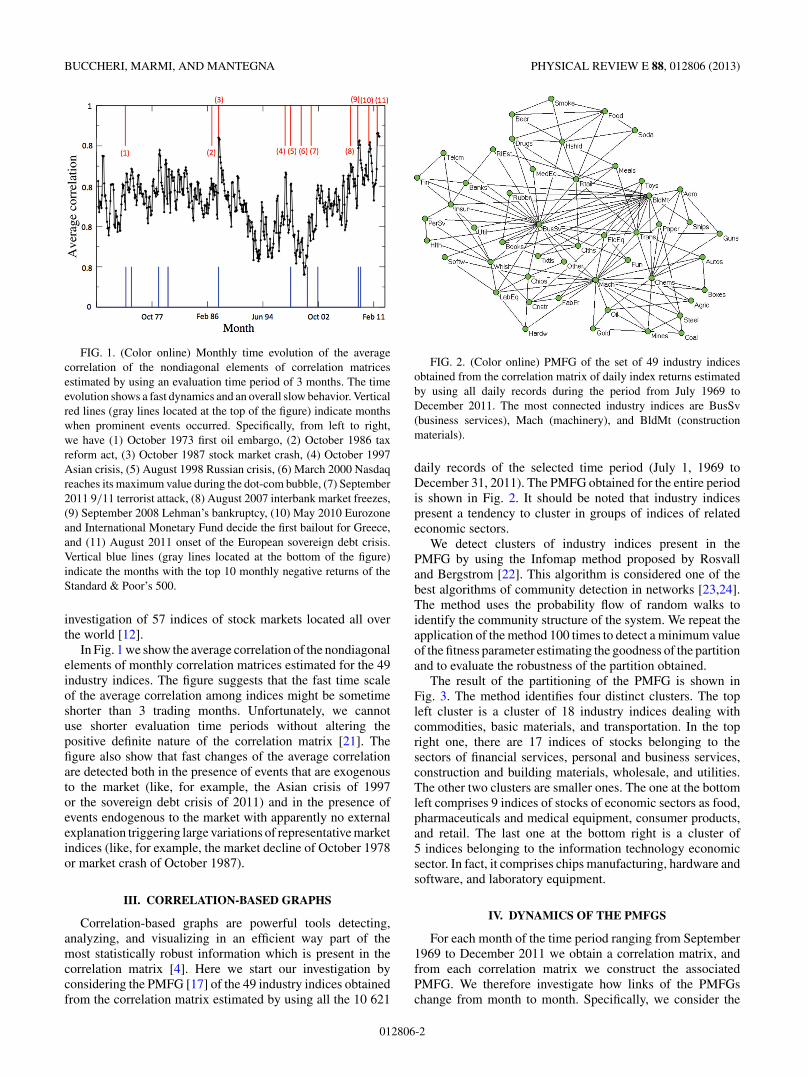
FIG. 1. (Color online) Monthly time evolution of the averagecorrelation of the nondiagonal elements of correlation matricesestimated by using an evaluation time period of 3 months. The timeevolution shows a fast dynamics and an overall slow behavior. Verticalred lines (gray lines located at the top of the figure) indicate monthswhen prominent events occurred. Specifically, from left to right,we have (1) October 1973 first oil embargo, (2) October 1986 taxreform act, (3) October 1987 stock market crash, (4) October 1997Asian crisis, (5) August 1998 Russian crisis, (6) March 2000 Nasdaqreaches its maximum value during the dot-com bubble, (7) September2011 9/11 terrorist attack, (8) August 2007 interbank market freezes,(9) September 2008 Lehman’s bankruptcy, (10) May 2010 Eurozoneand International Monetary Fund decide the first bailout for Greece,and (11) August 2011 onset of the European sovereign debt crisis.Vertical blue lines (gray lines located at the bottom of the figure)indicate the months with the top 10 monthly negative returns of theStandard & Poor’s 500.

investigation of 57 indices of stock markets located all overthe world [12].

In Fig. 1 we show the average correlation of the nondiagonalelements of monthly correlation matrices estimated for the 49industry indices. The figure suggests that the fast time scaleof the average correlation among indices might be sometimeshorter than 3 trading months. Unfortunately, we cannotuse shorter evaluation time periods without altering thepositive definite nature of the correlation matrix [21]. Thefigure also show that fast changes of the average correlationare detected both in the presence of events that are exogenousto the market (like, for example, the Asian crisis of 1997or the sovereign debt crisis of 2011) and in the presence ofevents endogenous to the market with apparently no externalexplanation triggering large variations of representative marketindices (like, for example, the market decline of October 1978or market crash of October 1987).

III. CORRELATION-BASED GRAPHS

Correlation-based graphs are powerful tools detecting,analyzing, and visualizing in an efficient way part of themost statistically robust information which is present in thecorrelation matrix [4]. Here we start our investigation byconsidering the PMFG [17] of the 49 industry indices obtainedfrom the correlation matrix estimated by using all the 10 621

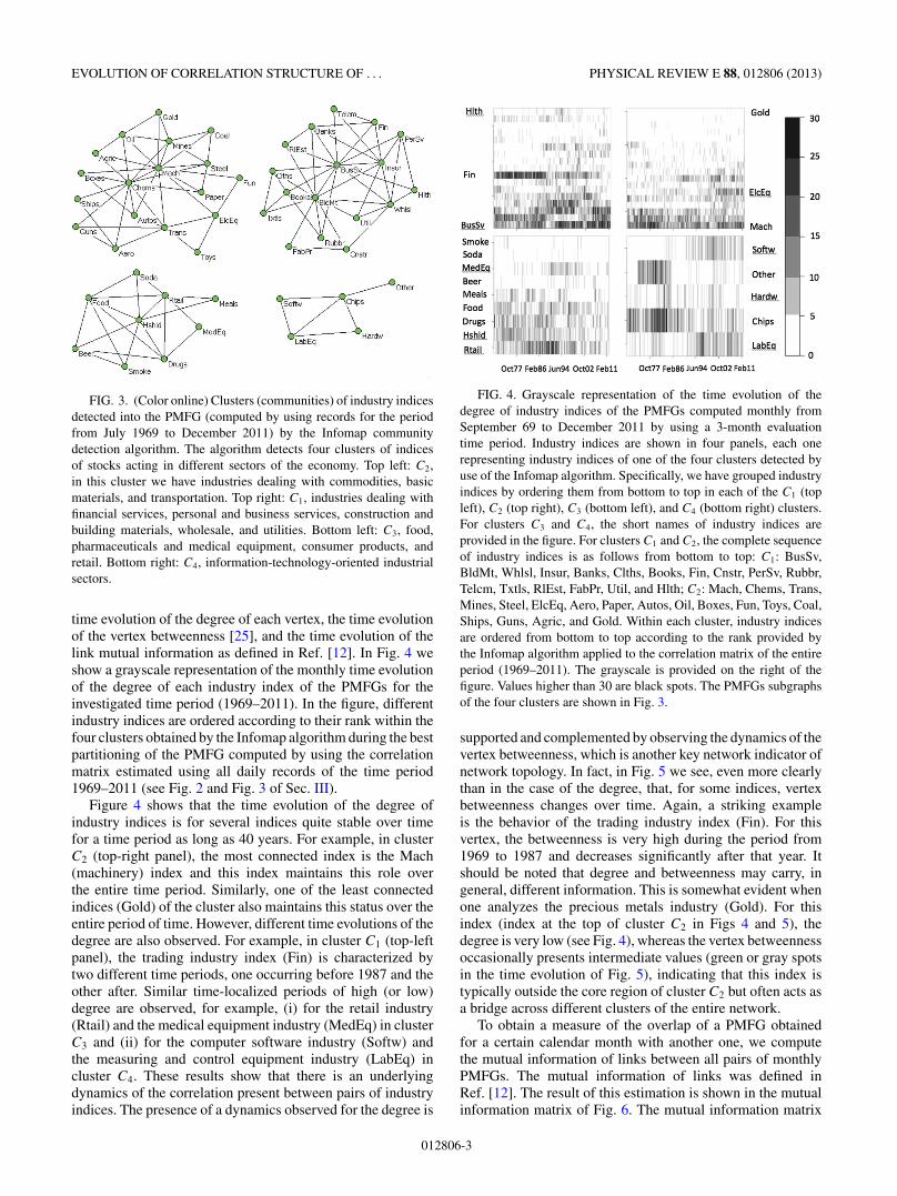
FIG. 2. (Color online) PMFG of the set of 49 industry indicesobtained from the correlation matrix of daily index returns estimatedby using all daily records during the period from July 1969 toDecember 2011. The most connected industry indices are BusSv(business services), Mach (machinery), and BldMt (constructionmaterials).

daily records of the selected time period (July 1, 1969 toDecember 31, 2011). The PMFG obtained for the entire periodis shown in Fig. 2. It should be noted that industry indicespresent a tendency to cluster in groups of indices of relatedeconomic sectors.

We detect clusters of industry indices present in thePMFG by using the Infomap method proposed by Rosvalland Bergstrom [22]. This algorithm is considered one of thebest algorithms of community detection in networks [23,24].The method uses the probability flow of random walks toidentify the community structure of the system. We repeat theapplication of the method 100 times to detect a minimum valueof the fitness parameter estimating the goodness of the partitionand to evaluate the robustness of the partition obtained.

The result of the partitioning of the PMFG is shown inFig. 3. The method identifies four distinct clusters. The topleft cluster is a cluster of 18 industry indices dealing withcommodities, basic materials, and transportation. In the topright one, there are 17 indices of stocks belonging to thesectors of financial services, personal and business services,construction and building materials, wholesale, and utilities.The other two clusters are smaller ones. The one at the bottomleft comprises 9 indices of stocks of economic sectors as food,pharmaceuticals and medical equipment, consumer products,and retail. The last one at the bottom right is a cluster of5 indices belonging to the information technology economicsector. In fact, it comprises chips manufacturing, hardware andsoftware, and laboratory equipment.

IV. DYNAMICS OF THE PMFGS

For each month of the time period ranging from September1969 to December 2011 we obtain a correlation matrix, andfrom each correlation matrix we construct the associatedPMFG. We therefore investigate how links of the PMFGschange from month to month. Specifically, we consider the

012806-2

EVOLUTION OF CORRELATION STRUCTURE OF . . . PHYSICAL REVIEW E 88, 012806 (2013)

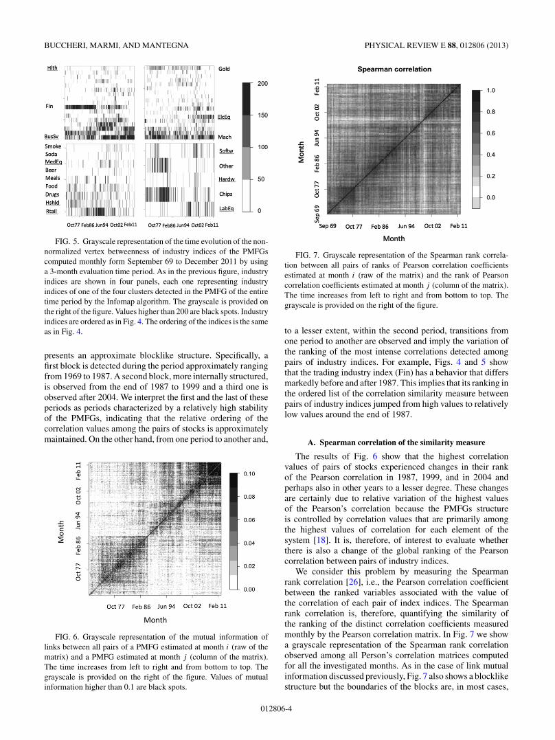
FIG. 3. (Color online) Clusters (communities) of industry indicesdetected into the PMFG (computed by using records for the periodfrom July 1969 to December 2011) by the Infomap communitydetection algorithm. The algorithm detects four clusters of indicesof stocks acting in different sectors of the economy. Top left: C2,in this cluster we have industries dealing with commodities, basicmaterials, and transportation. Top right: C1, industries dealing withfinancial services, personal and business services, construction andbuilding materials, wholesale, and utilities. Bottom left: C3, food,pharmaceuticals and medical equipment, consumer products, andretail. Bottom right: C4, information-technology-oriented industrialsectors.

time evolution of the degree of each vertex, the time evolutionof the vertex betweenness [25], and the time evolution of thelink mutual information as defined in Ref. [12]. In Fig. 4 weshow a grayscale representation of the monthly time evolutionof the degree of each industry index of the PMFGs for theinvestigated time period (1969–2011). In the figure, differentindustry indices are ordered according to their rank within thefour clusters obtained by the Infomap algorithm during the bestpartitioning of the PMFG computed by using the correlationmatrix estimated using all daily records of the time period1969–2011 (see Fig. 2 and Fig. 3 of Sec. III).

Figure 4 shows that the time evolution of the degree ofindustry indices is for several indices quite stable over timefor a time period as long as 40 years. For example, in clusterC2 (top-right panel), the most connected index is the Mach(machinery) index and this index maintains this role overthe entire time period. Similarly, one of the least connectedindices (Gold) of the cluster also maintains this status over theentire period of time. However, different time evolutions of thedegree are also observed. For example, in cluster C1 (top-leftpanel), the trading industry index (Fin) is characterized bytwo different time periods, one occurring before 1987 and theother after. Similar time-localized periods of high (or low)degree are observed, for example, (i) for the retail industry(Rtail) and the medical equipment industry (MedEq) in clusterC3 and (ii) for the computer software industry (Softw) andthe measuring and control equipment industry (LabEq) incluster C4. These results show that there is an underlyingdynamics of the correlation present between pairs of industryindices. The presence of a dynamics observed for the degree is

FIG. 4. Grayscale representation of the time evolution of thedegree of industry indices of the PMFGs computed monthly fromSeptember 69 to December 2011 by using a 3-month evaluationtime period. Industry indices are shown in four panels, each onerepresenting industry indices of one of the four clusters detected byuse of the Infomap algorithm. Specifically, we have grouped industryindices by ordering them from bottom to top in each of the C1 (topleft), C2 (top right), C3 (bottom left), and C4 (bottom right) clusters.For clusters C3 and C4, the short names of industry indices areprovided in the figure. For clusters C1 and C2, the complete sequenceof industry indices is as follows from bottom to top: C1: BusSv,BldMt, Whlsl, Insur, Banks, Clths, Books, Fin, Cnstr, PerSv, Rubbr,Telcm, Txtls, RlEst, FabPr, Util, and Hlth; C2: Mach, Chems, Trans,Mines, Steel, ElcEq, Aero, Paper, Autos, Oil, Boxes, Fun, Toys, Coal,Ships, Guns, Agric, and Gold. Within each cluster, industry indicesare ordered from bottom to top according to the rank provided bythe Infomap algorithm applied to the correlation matrix of the entireperiod (1969–2011). The grayscale is provided on the right of thefigure. Values higher than 30 are black spots. The PMFGs subgraphsof the four clusters are shown in Fig. 3.

supported and complemented by observing the dynamics of thevertex betweenness, which is another key network indicator ofnetwork topology. In fact, in Fig. 5 we see, even more clearlythan in the case of the degree, that, for some indices, vertexbetweenness changes over time. Again, a striking exampleis the behavior of the trading industry index (Fin). For thisvertex, the betweenness is very high during the period from1969 to 1987 and decreases significantly after that year. Itshould be noted that degree and betweenness may carry, ingeneral, different information. This is somewhat evident whenone analyzes the precious metals industry (Gold). For thisindex (index at the top of cluster C2 in Figs 4 and 5), thedegree is very low (see Fig. 4), whereas the vertex betweennessoccasionally presents intermediate values (green or gray spotsin the time evolution of Fig. 5), indicating that this index istypically outside the core region of cluster C2 but often acts asa bridge across different clusters of the entire network.

To obtain a measure of the overlap of a PMFG obtainedfor a certain calendar month with another one, we computethe mutual information of links between all pairs of monthlyPMFGs. The mutual information of links was defined inRef. [12]. The result of this estimation is shown in the mutualinformation matrix of Fig. 6. The mutual information matrix

012806-3

BUCCHERI, MARMI, AND MANTEGNA PHYSICAL REVIEW E 88, 012806 (2013)

FIG. 5. Grayscale representation of the time evolution of the non-normalized vertex betweenness of industry indices of the PMFGscomputed monthly form September 69 to December 2011 by usinga 3-month evaluation time period. As in the previous figure, industryindices are shown in four panels, each one representing industryindices of one of the four clusters detected in the PMFG of the entiretime period by the Infomap algorithm. The grayscale is provided onthe right of the figure. Values higher than 200 are black spots. Industryindices are ordered as in Fig. 4. The ordering of the indices is the sameas in Fig. 4.

presents an approximate blocklike structure. Specifically, afirst block is detected during the period approximately rangingfrom 1969 to 1987. A second block, more internally structured,is observed from the end of 1987 to 1999 and a third one isobserved after 2004. We interpret the first and the last of theseperiods as periods characterized by a relatively high stabilityof the PMFGs, indicating that the relative ordering of thecorrelation values among the pairs of stocks is approximatelymaintained. On the other hand, from one period to another and,

FIG. 6. Grayscale representation of the mutual information oflinks between all pairs of a PMFG estimated at month i (raw of thematrix) and a PMFG estimated at month j (column of the matrix).The time increases from left to right and from bottom to top. Thegrayscale is provided on the right of the figure. Values of mutualinformation higher than 0.1 are black spots.

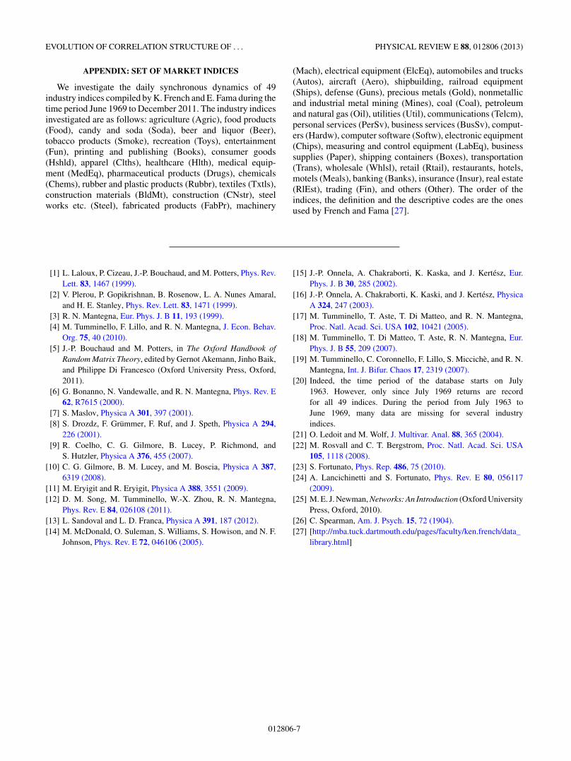
FIG. 7. Grayscale representation of the Spearman rank correla-tion between all pairs of ranks of Pearson correlation coefficientsestimated at month i (raw of the matrix) and the rank of Pearsoncorrelation coefficients estimated at month j (column of the matrix).The time increases from left to right and from bottom to top. Thegrayscale is provided on the right of the figure.

to a lesser extent, within the second period, transitions fromone period to another are observed and imply the variation ofthe ranking of the most intense correlations detected amongpairs of industry indices. For example, Figs. 4 and 5 showthat the trading industry index (Fin) has a behavior that differsmarkedly before and after 1987. This implies that its ranking inthe ordered list of the correlation similarity measure betweenpairs of industry indices jumped from high values to relativelylow values around the end of 1987.

A. Spearman correlation of the similarity measure

The results of Fig. 6 show that the highest correlationvalues of pairs of stocks experienced changes in their rankof the Pearson correlation in 1987, 1999, and in 2004 andperhaps also in other years to a lesser degree. These changesare certainly due to relative variation of the highest valuesof the Pearson’s correlation because the PMFGs structureis controlled by correlation values that are primarily amongthe highest values of correlation for each element of thesystem [18]. It is, therefore, of interest to evaluate whetherthere is also a change of the global ranking of the Pearsoncorrelation between pairs of industry indices.

We consider this problem by measuring the Spearmanrank correlation [26], i.e., the Pearson correlation coefficientbetween the ranked variables associated with the value ofthe correlation of each pair of index indices. The Spearmanrank correlation is, therefore, quantifying the similarity ofthe ranking of the distinct correlation coefficients measuredmonthly by the Pearson correlation matrix. In Fig. 7 we showa grayscale representation of the Spearman rank correlationobserved among all Person’s correlation matrices computedfor all the investigated months. As in the case of link mutualinformation discussed previously, Fig. 7 also shows a blocklikestructure but the boundaries of the blocks are, in most cases,

012806-4

EVOLUTION OF CORRELATION STRUCTURE OF . . . PHYSICAL REVIEW E 88, 012806 (2013)

FIG. 8. (Color online) Monthly time evolution of the first [black(top) line], second [red (middle) line], and third [green (bottom) line]eigenvalues of the correlation matrices computed by using a 3-monthevaluation time period. The dates of the most prominent spikes of thesecond eigenvalue are reported in the figure.

observed for times that differ from the ones characterizing themutual information (see Fig. 6). In fact, Fig. 7 shows majorboundaries among blocks in 1978, 1992, 1999, and 2001. Thebehavior during the time interval 1999–2001 markedly differsfrom any other past and future period, indicating that during thedot-com bubble the rank of the correlation coefficients amongindustry indices of the U.S. market significantly differed fromall other time periods. Figure 7 also shows that the rank of thePearson correlation coefficient among industry indices of theperiod 2001–2010 significantly differs from the rank observedin the past, especially when compared with the time periodprior to 1978.

V. SPECTRAL ANALYSIS OFTHE CORRELATION MATRICES

In the previous section, we have seen that both the highestvalues of the pair correlation and, more generally, the entireset of Pearson correlation coefficients have changed rankover time with abrupt changes in a few cases localized atspecific times. Here we continue the analysis of the propertiesof the Pearson correlation as a function of the time byinvestigating the spectrum of eigenvalues and eigenvectorsof the correlation matrices. In our analysis, we mainly focuson the time dynamics of the largest eigenvalues and oftheir corresponding eigenvectors. In Fig. 8 we show thetime evolution of the first, second, and third eigenvalue ofthe monthly correlation matrices. The time profile of thefirst eigenvalue is highly correlated with time profile of theaverage correlation (see Fig. 1) and, therefore, no additionalinformation can be easily extracted from him. The timeevolution of the second eigenvalue is more informative becauseit shows a few abrupt changes in specific periods of time. InFig. 8 we point out that biggest changes are observed duringApril–June 1999, March–May 2000, June–March 2001, andJuly–September 2008. The third eigenvalue has a more limitedexcursion; its mean value is equal to 1.82 and the standard

FIG. 9. Grayscale representation of the components of the firsteigenvector as a function of time (vertical axis). The direction ofthe eigenvector is selected by making positive the component of theBusSv industry index. Industry indices are ordered from bottom totop according to the clusters detected by the Infomap algorithm inthe unconditional PMFGs of Fig. 2. C1 to C4 are the clusters shownin Fig. 3.

deviation is 0.46. It therefore will be very difficult to extractthe information associated with this eigenvalue in a statisticallyreliable way. In summary, the first two eigenvalues are theonly large eigenvalues carrying information that is statisticallyreliable and easily distinguishable from fluctuations inducedin the estimation process by the limited number of recordsused to compute the correlation matrix [1].

We interpret the spikes observed in the time evolution of thesecond eigenvalue of the correlation matrix as an indication ofchanges occurring in the correlation matrix and, specifically,changes affecting the correlation of some specific sets ofindustry indices against all the others. This conclusion is alsoconsistent with the results obtained investigating the Spearmanrank correlation discussed in the previous section. It should benoted that the main spikes are localized during the time periodfrom April 1999 to March 2001, when the market experiencedthe strongest manifestation of the dot-com bubble (NASDAQindex reached its maximum value on March 10, 2000) andits deflation (NASDAQ index declined to half its value withina year from the maximum value). The other most prominentspike is observed for the time period July–September 2008,which was the hottest period of the 2008 financial crisis thatled to the Lehman’s failure of September 15, 2008. The spikesof the second eigenvalue therefore indicate two major crisesexperienced by the U.S. equity markets in recent years.

We investigate the nature of information present in thetwo eigenvalues by analyzing the profile of the eigenvectorsassociated with the two largest eigenvalues. In Fig. 9 we show agrayscale representation of the components of the eigenvectorassociated with the first eigenvalue for all 508 investigatedmonths. When the spectral analysis of a matrix is performed,the direction of the eigenvector is arbitrary. In the figure weselect the direction associated with a positive component of theeigenvector by setting positive the component of the business

012806-5

BUCCHERI, MARMI, AND MANTEGNA PHYSICAL REVIEW E 88, 012806 (2013)

FIG. 10. (Color online) Grayscale representation of the compo-nents of the second eigenvector as a function of time. The directionof the eigenvector is selected by making positive the componentof the BusSv index. Market indices are ordered from bottom to topaccording to the clusters detected by the Infomap algorithm in theunconditional PMFGs of Fig. 2. C1 to C4 are the clusters shown inFig. 3. The top panel describes the entire time period investigated,whereas the bottom panel refers to the dot-com time period fromMarch 1999 to May 2001.

services industry index (BusSv). The eigenvector componentsare almost all positive, indicating the presence of a commonfactor driving all industry indices. The only significant excep-tion is the last industry index of cluster C2. This industry indexis the precious metals industry index (Gold).

The time evolution of the components of the eigenvector ofthe second eigenvalue has a less-straightforward interpretation.During the time period before 1987, clusters C1 and C3 showvalues of the components of the eigenvector with valuespreferentially positive or negative, respectively (see the toppanel of Fig. 10). After 1987 the general behavior is muchmore complex, although some local regularities emerge. Forexample, one prominent case is observed during the periodfrom March 1999 to April 2001, i.e., the period when thesecond eigenvalue shows prominent spikes. During this timeperiod, the values of the components of the eigenvector ofindustry indices of the C4 cluster assume, with the only

exception being the index Other, very high positive values,while the large majority of all other industry indices assumevalues close to zero or that are negative (see the bottom panelof Fig. 10). This is a direct manifestation of the fact that,during that period of time, there was a strong decoupling of thecorrelation present between industry indices directly relatedto information technology, computers (Hardw), computersoftware (Softw), electronic equipment (Chips), measuringand control equipment(LabEq), and the rest of indices.

In summary, our analysis of the dynamics of the first twolargest eigenvalues shows a strong alteration of the value ofeigenvalues for the time period associated with two of themost prominent market periods of the past 40 years, whichare the dot-com bubble and the peak of the subprime crisis.Concerning the relevance of the second eigenvalue in termsof explained variance, it is worth noting that, in absoluteterms, the second eigenvalue explains a maximal amount ofapproximately 16% of the variance during the two periodsof time discussed here. Moreover, in relative terms the twoperiods differ substantially because for the dot-com period thefirst eigenvalue explains approximately 31% of the variance,whereas, during the 2008–2009 crisis, the first eigenvalueexplains roughly 70% of the variance. In other words, the2008–2009 crisis affects all the industry indices, whereasthe dot-com bubble was primarily affectcting the informationtechnology industry sector.

VI. CONCLUSIONS

In this paper, we investigate the dynamics of correlationpresent among pairs of industry indices of U.S. stock tradedin U.S. markets. The study is performed by using 49 industryindex time series computed by K. French and E. Fama since1962. By investigating this set of industry indices over aperiod of time spanning more than 40 years, we discoverthat the correlation between industry indices presents botha fast and a slow dynamics. The slow dynamics indicatesthat a different degree of diversification of the investment ispossible in different periods of time and that the time scaleof these changes is at least as slow as 5 years. On top ofthis slow dynamics, we also detect a fast dynamics associatedwith exogenous or endogenous market events. Specifically, bycomputing the correlation matrix for each trading month usinga 3-month evaluation time period, we show that the correlationmatrix presents both very long periods of time during whichthe relative rank of Pearson correlation coefficients betweenpairs of industry indices is rather stable and periods when thereis a significant modification of relative correlation in relativelyshort periods of time. Two major examples of these abruptchanges are observed during the dot-com bubble (March 1999to April 2001) and during the period of highest impact of thesubprime crisis (August 2008 to August 2009).

ACKNOWLEDGMENTS

The research leading to these results has received partialfunding from the European Union, Seventh Framework Pro-gramme FP7/2007-2013, under Grant No. CRISIS-ICT-2011-288501.

012806-6

EVOLUTION OF CORRELATION STRUCTURE OF . . . PHYSICAL REVIEW E 88, 012806 (2013)

APPENDIX: SET OF MARKET INDICES

We investigate the daily synchronous dynamics of 49industry indices compiled by K. French and E. Fama during thetime period June 1969 to December 2011. The industry indicesinvestigated are as follows: agriculture (Agric), food products(Food), candy and soda (Soda), beer and liquor (Beer),tobacco products (Smoke), recreation (Toys), entertainment(Fun), printing and publishing (Books), consumer goods(Hshld), apparel (Clths), healthcare (Hlth), medical equip-ment (MedEq), pharmaceutical products (Drugs), chemicals(Chems), rubber and plastic products (Rubbr), textiles (Txtls),construction materials (BldMt), construction (CNstr), steelworks etc. (Steel), fabricated products (FabPr), machinery

(Mach), electrical equipment (ElcEq), automobiles and trucks(Autos), aircraft (Aero), shipbuilding, railroad equipment(Ships), defense (Guns), precious metals (Gold), nonmetallicand industrial metal mining (Mines), coal (Coal), petroleumand natural gas (Oil), utilities (Util), communications (Telcm),personal services (PerSv), business services (BusSv), comput-ers (Hardw), computer software (Softw), electronic equipment(Chips), measuring and control equipment (LabEq), businesssupplies (Paper), shipping containers (Boxes), transportation(Trans), wholesale (Whlsl), retail (Rtail), restaurants, hotels,motels (Meals), banking (Banks), insurance (Insur), real estate(RlEst), trading (Fin), and others (Other). The order of theindices, the definition and the descriptive codes are the onesused by French and Fama [27].

[1] L. Laloux, P. Cizeau, J.-P. Bouchaud, and M. Potters, Phys. Rev.Lett. 83, 1467 (1999).

[2] V. Plerou, P. Gopikrishnan, B. Rosenow, L. A. Nunes Amaral,and H. E. Stanley, Phys. Rev. Lett. 83, 1471 (1999).

[3] R. N. Mantegna, Eur. Phys. J. B 11, 193 (1999).[4] M. Tumminello, F. Lillo, and R. N. Mantegna, J. Econ. Behav.

Org. 75, 40 (2010).[5] J.-P. Bouchaud and M. Potters, in The Oxford Handbook of

Random Matrix Theory, edited by Gernot Akemann, Jinho Baik,and Philippe Di Francesco (Oxford University Press, Oxford,2011).

[6] G. Bonanno, N. Vandewalle, and R. N. Mantegna, Phys. Rev. E62, R7615 (2000).

[7] S. Maslov, Physica A 301, 397 (2001).[8] S. Drozdz, F. Grummer, F. Ruf, and J. Speth, Physica A 294,

226 (2001).[9] R. Coelho, C. G. Gilmore, B. Lucey, P. Richmond, and

S. Hutzler, Physica A 376, 455 (2007).[10] C. G. Gilmore, B. M. Lucey, and M. Boscia, Physica A 387,

6319 (2008).[11] M. Eryigit and R. Eryigit, Physica A 388, 3551 (2009).[12] D. M. Song, M. Tumminello, W.-X. Zhou, R. N. Mantegna,

Phys. Rev. E 84, 026108 (2011).[13] L. Sandoval and L. D. Franca, Physica A 391, 187 (2012).[14] M. McDonald, O. Suleman, S. Williams, S. Howison, and N. F.

Johnson, Phys. Rev. E 72, 046106 (2005).

[15] J.-P. Onnela, A. Chakraborti, K. Kaska, and J. Kertesz, Eur.Phys. J. B 30, 285 (2002).

[16] J.-P. Onnela, A. Chakraborti, K. Kaski, and J. Kertesz, PhysicaA 324, 247 (2003).

[17] M. Tumminello, T. Aste, T. Di Matteo, and R. N. Mantegna,Proc. Natl. Acad. Sci. USA 102, 10421 (2005).

[18] M. Tumminello, T. Di Matteo, T. Aste, R. N. Mantegna, Eur.Phys. J. B 55, 209 (2007).

[19] M. Tumminello, C. Coronnello, F. Lillo, S. Micciche, and R. N.Mantegna, Int. J. Bifur. Chaos 17, 2319 (2007).

[20] Indeed, the time period of the database starts on July1963. However, only since July 1969 returns are recordfor all 49 indices. During the period from July 1963 toJune 1969, many data are missing for several industryindices.

[21] O. Ledoit and M. Wolf, J. Multivar. Anal. 88, 365 (2004).[22] M. Rosvall and C. T. Bergstrom, Proc. Natl. Acad. Sci. USA

105, 1118 (2008).[23] S. Fortunato, Phys. Rep. 486, 75 (2010).[24] A. Lancichinetti and S. Fortunato, Phys. Rev. E 80, 056117

(2009).[25] M. E. J. Newman, Networks: An Introduction (Oxford University

Press, Oxford, 2010).[26] C. Spearman, Am. J. Psych. 15, 72 (1904).[27] [http://mba.tuck.dartmouth.edu/pages/faculty/ken.french/data_

library.html]

012806-7