Euro area inflation persistence in an estimated nonlinearDSGE model∗

Gianni Amisano†

Università di BresciaOreste Tristani‡

European Central Bank

8 December 2005Preliminary and incomplete: please do not quote.

Abstract

We estimate the approximate nonlinear solution of a small DSGE model usingBayesian methods. Our results, based on euro area data, suggest that this approchdelivers sharper inference compared to the estimation of the linearised solution. Thenonlinear model can also account for richer economic dynamics. The impulse responsesof inflation to structural shocks may vary depending on initial conditions: they aremuch more persistent when inflation is significantly above its long run equilibriumlevel.

JEL classification:Keywords: DSGE models, policy rules, inflation persistence, second order ap-

proximations, particle filter, Bayesian estimation.

∗The opinions expressed are personal and should not be attributed to the European Central Bank.†Address: Università di Brescia, Facoltà di Economia, Via S. Faustino 74/B, I - 25122 Brescia, Italy.

E-mail: amisano@eco.unibs.it.‡Address: European Central Bank, DG Research, Kaiserstrasse 29, D - 60311, Frankfurt, Germany.

E-mail: oreste.tristani@ecb.int.

1

1 Introduction

Dynamic stochastic general equilibrium (DSGE) models have become popular tools for

monetary policy analysis. The central feature of these models, emphasised in the the-

oretical work of Yun (1996) and Woodford (2003), is the presence of nominal rigidities

in the adjustment of goods prices. More recently, a number of additional frictions have

been introduced in the basic sticky-price framework and the resulting models have been

successfully taken to the data (see e.g. Christiano, Eichenbaum and Evans, 2005; Smets

and Wouters, 2003).

In all cases, however, what is estimated is only the reduced form emerging from the

solution of a linearised version of those models. This approach has obvious advantages in

terms of simplicity and possibility of comparison to other well-known empirical tools, such

as VARs. There are a number of reasons, however, to also be interested in exploring the

implications of the many nonlinear features built in DSGE models. Amongst these, three

such reasons can be mentioned here.

The first one is that they are more suited to characterise macroeconomic dynamics in

presence of large deviations from the steady state. Even in relatively short samples of 20

or 25 years, such as the post-1979 sample typically explored in empirical monetary policy

analyses after the work of Clarida, Galí and Gertler (1998, 2000), euro area inflation has

reached a maximum and minimum of 12.0 and 0.6 percent, respectively, compared to an

average of 4.2 percent. By construction, a linearised model is not suited to explain such

large deviations and it might deliver distorted estimates, at least in principle, if forced to

do so.

To provide a more concrete example, it is conceivable that inflation persistence should

depend on its distance from the steady state. Small deviations could be characterised by a

relatively small degree of persistence, but the persistence could become more pronounced

in case of larger deviations, which would more easibly become entrenched in expectations.

This economic feature could be captured by higher-order terms in a nonlinear solution,

terms which, by construction, would start playing a nonnegligible role only when large

deviations from steady state do take place. A linearised model, on the contrary, would

be forced to account for all observed dynamics with linear terms. It could therefore

deliver estimates of inflation persistence that are biased upwards for small deviations and

downwards for large deviations from the steady state. We test this conjecture explicitly

2

in our estimations.

The second reason to be interested in nonlinear models is empirical, since nonlinear

models are likely to provide sharper estimates than their linearised counterparts. More

specifically, the nonlinearities of a model can be seen as additional testable implications

compared to those characterising the linearised version of the same model. A straigh-

forward example can be made for the case of solutions obtained through second-order

perturbation methods. These approximate solutions imply that the variance of exoge-

nous shocks have an impact on the unconditional means of observable variables. This

link amounts to a restriction on the size of those variances. This restriction is ignored in

linearised solutions.

A more general empirical advantage of the estimation of nonlinear models is highlighted

by Fernandez-Villaverde, Rubio-Ramirez and Santos (2005). The paper shows that the

approximation errors of a model are compounded when constructing the likelihood func-

tion. As a result, a model solved up to a second-order approximation is the minimum

requirement to obtain a first order approximation to the true likelihood function of the

nonlinear model.

The third reason to be interested in nonlinear models is related to the possibility

of exploring the asset price implications of macroeconomic models. The notions of risk

and risk aversion only assume concrete meaning in nonlinear models. Conversely, linear

models deliver by construction equal returns on all assets regardles of their riskiness. The

availability of nonlinear solutions is therefore a necessary condition to analyse satisfactorily

the implications of any macroeconomic model for the term structure of interest rates and

equity prices. These implications can be of interest from an asset pricing perspective, but

also from a purely macroeconomic perspective. Exploring the asset price implications of

macroeconomic models can in fact be a powerful test of those models, whic highlights their

weaknesses and can act as a catalist for further improvements.

The main objective of this paper is to explore the empirical implications of a small

DSGE model of the euro area solved using second-order perturbation methods. While

other authors have provided results based on second or higher order approximation meth-

ods using simulated data (e.g. An and Schorfeide, 2005; Fernandez-Villaverde and Rubio-

Ramirez, 2004), ours is, to our knowledge, the first paper which takes the second-order

approximation of a DSGE model directly to the data.

3

Our preliminary results show that the nonlinear version of DSGE models provides

sharper inference and accounts for richer economic dynamics compared to linearised ver-

sions. Concerning the persistence of euro area inflation, we show, using two different

model-specifications, that significant differences can be found between linear and nonlin-

ear solutions.

The rest of the paper is organised as follows. Section 2 provides a broad description

of the two models that we estimate in the empirical section. The main difference between

those models concerns the behaviour of monetary policy. While always following a Taylor-

type rule, the central bank is assumed to have a stationary stochastic inflation target in

the first case and an integrated target in the second case. Section 3 discusses briefly the

solution method. It is well-known that approximate nonlinear solutions can be computed

using a variety of methods (see Aruoba, Fernandez-Villaverde and Rubio-Ramirez, 2003).

We focus on second-order perturbation methods, because they are direct extentions of

standard linearisations and because they are fast to implement. The estimation method-

ology is presented next, in Section 4, with particular emphasis on the construction of the

likelihood function, which is performed using the particle filter. We also discuss briefly

some of the choices available to the researcher in this context and the importance of a

plausible specification of the priors for the variance of the shocks. Section 5 presents the

estimation results. More specifically, we discuss the differences between estimates obtained

through linear and nonlinear versions of each model, in terms of both posterior densities

for the parameters and conditional and unconditional moments. We then draw implica-

tions for the estimated degree of inflation persistence and compare this to previous results

in the literature. Section 6 concludes.

2 The theoretical framework

One of the conclusions of the "Inflation Persistence Network" (IPN) coordinated by the

European Central Bank is that the estimated persistence of aggregate euro area inflation

changes depending on one key hypothesis (see e.g. Angeloni et al., 2005), namely whether

shifts in the mean of inflation are, or not, accounted for. Empirical estimates of inflation

persistence are high in the first case, while they fall considerably in the second. For

example, Bilke (2004) argues that a structural break in French CPI inflation occurred in the

4

mid-eighties. Controlling for this break, both aggregate and sectoral inflation persistence

are stable and low. Levin and Piger (2004) also find strong evidence for a break in the

mean of inflation in the late 1980s or early 1990s for twelve industrial countries. Allowing

for such break, the inflation measures generally exhibit relatively low inflation persistence.

Similar results are obtained by Corvoisier and Mojon (2004) for most OECD countries.

Dossche and Everaert (2004) find similar results when they allow for shifts in the inflation

target in the form of a random walk.

By and large, the existence of shifts in the mean of inflation has been tested within

statistical or reduced-form frameworks (see e.g. Levin and Piger, 2004; Corvoisier and

Mojon, 2004). As a result, it could be argued that there are two difficulties with the

interpretation of these results. First, it remains unclear whether the hypothesis of one or

more shifts in the mean of inflation would be rejected within a structural model. For this

purpose, it would be desirable to construct a DSGE model where the possibility of shifts

in the inflation mean is allowed for and then tested empirically. Secondly, the reasons for

a potential shift in the inflation mean are left unspecified.

To address these issues, we explore the empirical plausibility of two variants of a simple

DSGE model of inflation and output dynamics. The first one is a benchmark model

which embodies the assumption of no permanent shifts in the average inflation rate. In

this framework, we investigate whether the nonlinearities of the model can explain the

persistently high inflation rates observed in the first part of our sample as reflecting the

impact of higher order terms in the solution, terms which play instead a negligible role

when inflation is low (and presumably close to the steady state).

We the compare these results to those obtained within a model where smooth shifts

in the mean of inflation are allowed for through an integrated inflation target. We study

the relevance of the nonlinear aspects of the model also in this case — even if one would

expect them to be less relevant, because time variations in the mean should imply that

deviations from the mean are normally small.

In the rest of this section, we present in more detail the main features of the micro-

economic environment, that are common to the three models, and the three policy rules

which represent the main differences across the three specifications.

5

2.1 A simple DSGE model

The model is based on the framework developed by Woodford (2003) and extended in a

number of directions by Christiano, Eichenbaum and Evans (2005).

Consumers maximize the discounted sum of the period utility

U (Ct,Ht, Lt) = edt(Ct − hCt−1)

1−γ

1− γ−Z 1

0χLt (i)

φ di (1)

where C is a consumption index satisfying

C =

µZ 1

0C (i)

θ−1θ

¶ θθ−1

, (2)

Ht = hCt−1 is the habit stock, L (i) are hours of labour provided to firm i and dt is a

serially correlated preference shock

dt = ρddt−1 + εdt , εdt ∼ N¡0, σ2d

¢. (3)

For consistency with Smets and Wouters (2003) and Christiano, Eichenbaum and

Evans (2005), habit formation is modelled in difference form. However, habit is inter-

nal, so that households care about their own lagged consumption.

The households’ budget constraint is given by

PtCt +Bt 6µ1− τ t

1 + τ t

¶Z 1

0wt (i)Lt (i) di+

Z 1

0Ξt (i) di+Wt (4)

with the price level Pt defined as the minimal cost of buying one unit of Ct, hence equal

to

Pt =

µZ 1

0p (i)1−θ

¶ 11−θ

. (5)

In the budget constraint, Bt denotes end of period holdings of a complete portfolio of

state contingent assets. Wt denotes the beginning of period value of the assets, wt (i) is the

nominal wage rate, Lt (i) is the supply of labor to firm i and Ξt (i) are the profits received

from investment in firm i. Following Steinsson (2003), we also introduce a stochastic

income tax, which will lead to a trade-off between inflation and the output gap. We write

the tax rate as τ t1+τ t

to ensure that the total tax is bounded between 0 and 1, given that

log τ t = (1− ρτ ) τ + ρτ log τ t−1 + ετt , ετt ∼ N¡0, σ2τ

¢. (6)

6

The first order conditions w.r.t intertemporal aggregate consumption allocation and

labour supply can be written asµ1− τ t

1 + τ t

¶wt (i)

Pt=

φχL (i)φ−1

Λt

Λt = edt (Ct − hCt−1)−γ − βhEt

hedt+1 (Ct+1 − hCt)

−γi

(7)

1

It= Et

∙β

PtPt+1

Λt+1Λt

¸.

where It is the gross nominal interest rate.

Turning to the firms problem, the production function is given by

Yt (i) = AtL (i)α , At = A

ρat−1e

εat (8)

where At is a technology shock and εat is a normally distributed shock with constant

variance σ2a.

We assume Calvo (1983) contracts, so that firms face a constant probability ζ of being

unable to change their price at each time t. Firms will take this constraint into account

when trying to maximize expected profits, namely

maxP it

Et

∞Xs=t

ζs−tβsPtPt+s

Λt+sΛt

¡P isY

is − TCi

s

¢, (9)

where TC denotes total costs and, as in Smets and Wouters (2003), firms not changing

prices optimally are assumed to modify them using a rule of thumb that indexes them

partly to lagged inflation and partly to steady-state inflation Π, namely P it

¡Π¢1−ι ³Ps−1

Pt−1

´ι,

where 0 ≤ ι ≤ 1. The exception is when we assume an integrated inflation target and

steady state inflation is not defined. In that case, we set ι = 1. We introduce indexation

in the model for two reasons. First, aggregate inflation will be driven to some extent by

lagged inflation, which is an empirically plausible hypothesis — though not immediately

consistent with the microeconomic evidence. Second, firms not allowed to update their

prices optimally for a long time will still find themselves with a price which is not too far

from the optimum.

Under the assumption that firms are perfectly symmetric in all other respects than

the ability to change prices, all firms that do get to change their price will set it at the

same optimal level P ∗t . The first order conditions of the firms’ problem can be written

7

recursively as implying (see Hördahl, Tristani and Vestin, 2005)µP ∗tPt

¶1−θ(1− φα)

=φχθ

α (θ − 1)K2,t

K1,t

K2,t =A− φα

t³1− τ t

1+τ t

´Λt

Yφαt +EtζΠ

−θ φα(1−ι)

βPtPt+1

Λt+1Λt

K2,t+1Π−θ φ

αι

t Π1+θ φ

αt+1(10)

K1,t = Yt +EtζΠ(1−θ)(1−ι)

βPtPt+1

Λt+1Λt

K1,t+1Π(1−θ)ιt Πθt+1

where Πt is the inflation rate defined as Πt ≡ PtPt−1

and

P ∗tPt=

⎛⎜⎝1− ζ³Π1−ιΠι

t−1Πt

´1−θ(1− ζ)

⎞⎟⎠1

1−θ

(11)

expresses the optimal price at time t as a function of aggregate variables.1

2.2 Two Taylor rules

Equations (3), (6)-(8), (10)-(11) describe aggregate economic dynamics. We close the

model with a Taylor rule with interest rate smoothing. A key decision that has to be

taken in the specification of the rule concerns the inflation target. Since inflation displays

a noticeable downward trend over the sample period, the assumption of a constant target

is not very appealing. In empirical applications, it is therefore often assumed that the

decline in inflation corresponds to a decline in the inflation target. This is also what we

do here. However, this assumption is likely to have important implications in terms of

the persistence of inflation. In order to explore this issue, we analyse two variants of the

policy rule.

The first rule assumes that the inflation target follows a stationary AR(1) process. In

this case, the idea is that the long run target of the central bank is actually constant, but

that there are shifts in the horizon at which the central bank tries to get inflation back

to that long run level. If the target is temporarily high when inflation is high, then the

central bank is willing to tolerate a slow return to the long run target. If, instead, there

are no changes in the long run target when inflation is high, inflation will be brought back

on target more quickly.

1Similar expressions are derived in Ascari (2004), for the case without indexation.

8

In logarithmic terms (lower case letters), the first rule takes the form

it = (1− ρI) (π − lnβ) + ψπ (πt − π∗t ) + ψy (yt − ynt ) + ρIit−1 + εit (12)

π∗t = (1− ρπ)π + ρππ∗t−1 + επ

∗t (13)

where it is the logarithm of the gross nominal interest rate, π∗t is the inflation target, uit is a

policy shock and ynt is the logarithm of the level of natural output. The innovations εit and

επ∗

t are white noise with variances σ2i and σ2π∗ , respectively. In this model, considerable

deviations from the mean of inflation can arise from short-term movements in the inflation

target. The model solved using the first policy rule is dubbed MODEL1.

The second policy rule is identical to the first, except for the property that the inflation

target becomes integrated (and the steady state level of the interest rate is modified

accordingly)

it = (1− ρI)¡(π∗t − lnβ) + ψπ (πt − π∗t ) + ψy (yt − ynt )

¢+ ρIit−1 + εit (14)

π∗t = π∗t−1 + επ∗

t (15)

In this case, smooth changes of the mean occur over time as the central bank target

is revised. The idea here is that the inflation target process captures true shifts in the

objective of the central bank. Given the slow decline in inflation over our sample period,

this should supposedly reflect a shift in public preferences in favour of lower and lower

inflation levels. The integrated inflation target induces a non-stationary behaviour also

in actual inflation and the nominal interest rate. These nominal variables are also co-

integrated, so that the model can be written in stationary form in terms of the rate of

growth of inflation, ∆πt = πt − πt−1, and the deflated inflation target and interest rate,

defined as eπ∗t = π∗t − πt and eit = it − πt, respectively. This model is dubbed MODEL2.

3 Second-order approximate solution

We solve the model using a second order approximation around the non-stochastic steady

state. The model dynamics will then be described by two systems of equations: a quadratic

law of motion for the predetermined variables of the model and a quadratic relationship

linking each non-predetermined variable to the predetermined variables.

The solution is obtained numerically. A few methods have been proposed in the liter-

ature, including those in Schmitt-Grohé and Uribe (2002) and Kim et al. (2003). For our

9

applications we select the implementation proposed by Klein (2005), that has the advan-

tage of being relatively faster. Speed is particularly important for estimation, since the

model needs to be solved at every evaluation of the likelihood. For this reason, we also

rely on analytical derivatives to evaluate the second order terms of the approximation.

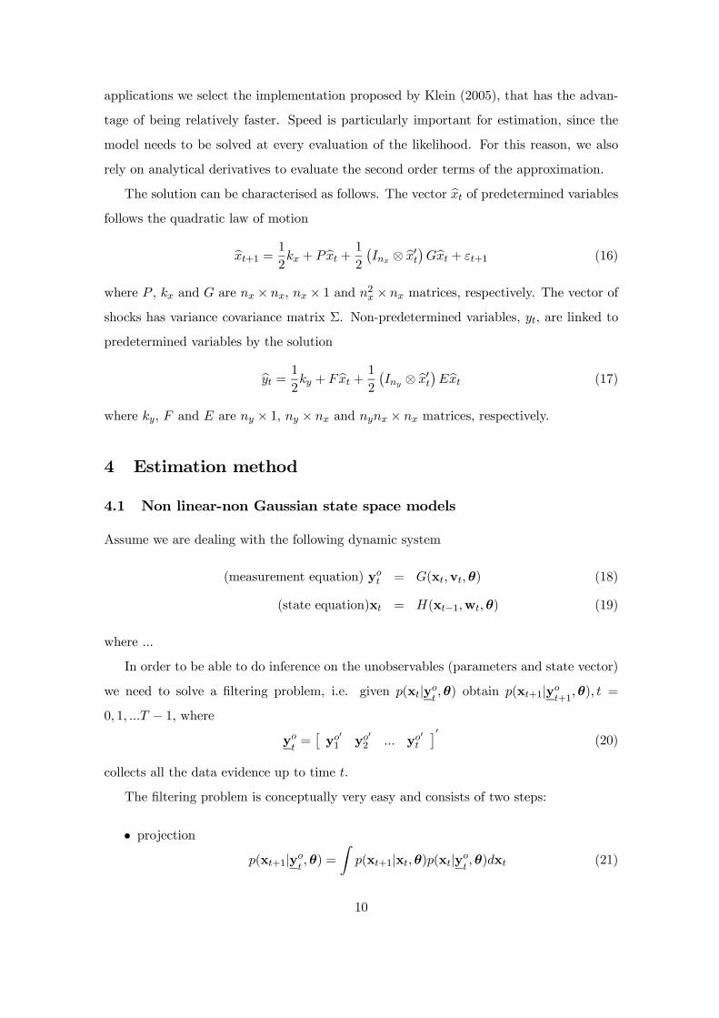
The solution can be characterised as follows. The vector bxt of predetermined variablesfollows the quadratic law of motion

bxt+1 = 1

2kx + Pbxt + 1

2

¡Inx ⊗ bx0t¢Gbxt + εt+1 (16)

where P , kx and G are nx × nx, nx × 1 and n2x × nx matrices, respectively. The vector of

shocks has variance covariance matrix Σ. Non-predetermined variables, yt, are linked to

predetermined variables by the solution

byt = 1

2ky + F bxt + 1

2

¡Iny ⊗ bx0t¢Ebxt (17)

where ky, F and E are ny × 1, ny × nx and nynx × nx matrices, respectively.

4 Estimation method

4.1 Non linear-non Gaussian state space models

Assume we are dealing with the following dynamic system

(measurement equation) yot = G(xt,vt,θ) (18)

(state equation)xt = H(xt−1,wt,θ) (19)

where ...

In order to be able to do inference on the unobservables (parameters and state vector)

we need to solve a filtering problem, i.e. given p(xt|yot ,θ) obtain p(xt+1|yot+1,θ), t =

0, 1, ...T − 1, where

yot=£yo

01 yo

02 ... yo

0t

¤0(20)

collects all the data evidence up to time t.

The filtering problem is conceptually very easy and consists of two steps:

• projection

p(xt+1|yot ,θ) =Z

p(xt+1|xt,θ)p(xt|yot ,θ)dxt (21)

10

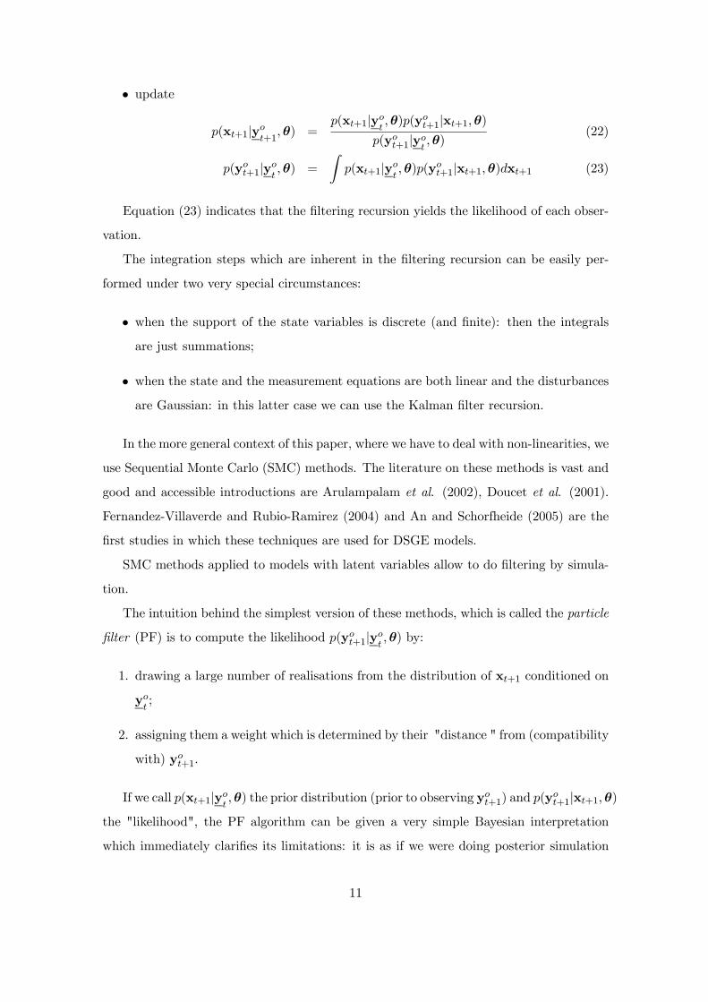
• update

p(xt+1|yot+1,θ) =p(xt+1|yot ,θ)p(y

ot+1|xt+1,θ)

p(yot+1|yot ,θ)(22)

p(yot+1|yot ,θ) =

Zp(xt+1|yot ,θ)p(y

ot+1|xt+1,θ)dxt+1 (23)

Equation (23) indicates that the filtering recursion yields the likelihood of each obser-

vation.

The integration steps which are inherent in the filtering recursion can be easily per-

formed under two very special circumstances:

• when the support of the state variables is discrete (and finite): then the integrals

are just summations;

• when the state and the measurement equations are both linear and the disturbances

are Gaussian: in this latter case we can use the Kalman filter recursion.

In the more general context of this paper, where we have to deal with non-linearities, we

use Sequential Monte Carlo (SMC) methods. The literature on these methods is vast and

good and accessible introductions are Arulampalam et al. (2002), Doucet et al. (2001).

Fernandez-Villaverde and Rubio-Ramirez (2004) and An and Schorfheide (2005) are the

first studies in which these techniques are used for DSGE models.

SMC methods applied to models with latent variables allow to do filtering by simula-

tion.

The intuition behind the simplest version of these methods, which is called the particle

filter (PF) is to compute the likelihood p(yot+1|yot ,θ) by:

1. drawing a large number of realisations from the distribution of xt+1 conditioned on

yot;

2. assigning them a weight which is determined by their "distance " from (compatibility

with) yot+1.

If we call p(xt+1|yot ,θ) the prior distribution (prior to observing yot+1) and p(y

ot+1|xt+1,θ)

the "likelihood", the PF algorithm can be given a very simple Bayesian interpretation

which immediately clarifies its limitations: it is as if we were doing posterior simulation

11

drawing from the prior and then using the likelihood as weights. This is a very easy pro-

cedure to implement but hardly a computationally efficient one in the case the likelihood

is much more concentrated than the prior.

The PF works as follows: imagine that at time t we have the availability of a large

number N of draws to approximate p(xt|yot ,θ) (we have a so called swarm of particles):³x(i)t , w

(i)t

´, i = 1, 2, ...,N (24)

Each particle is endowed with a weight w(i)t which might be the result of the fact that

each x(i)t might have been drawn from a distribution q(xt) which does not coincide with

p(xt|yot ,θ)2:

w(i)t =

p(x(i)t |yot ,θ)q(x

(i)t )

(25)

Note that it is possible to use this sample to compute the expected value of any function

f of xt in two different ways:

• via direct Importance Sampling (IS):

Ehf(x

(i)t )|yot ,θ

i≈

NXi=1

w(i)t f(x

(i)t )

NXi=1

w(i)t

(26)

• Alternatively it is possible to resample the x(i)t drawing N times (with reimmission)

from empirical distribution of the x(i)t , with probabilities given by w(i)t . In this way

we obtain a modified sample ³x(j)t , 1

´, j = 1, 2, ..., N (27)

which can be directly used to form the desired estimate:

Ehf(x

(i)t )|yot ,θ

i≈

NXj=1

f(x(j)t )

N(28)

The swarm of particles³x(i)t , w

(i)t

´, i = 1, 2, ..., N, can be used to perform filtering by

simulation. The easiest way to do this is to construct the so called particle filter (PF)

2 In this case we have the so-called Importance sampling. See Geweke 1989.

12

algorithm which consists of two simple steps. Assuming to have a swarm of particles with

perfectly even weights (w(j)t = 1, j = 1, 2, ..., N), the simulation filtering consists in two

steps:

• projection

p(xt+1|yot+1,θ) ≈

NXj=1

p(xt+1|x(j)t )

N(29)

This step is empirically performed by taking each particle x(j)t and drawing x(j)t+1from

the distribution

p(xt+1|x(j)t ,θ) (30)

This amounts to simulate from the state equation. In this way, the projection dis-

tribution is approximated by the sample³x(j)t+1, 1

´, j = 1, 2, ..., N (31)

• Update: we take into account that we have drawn from p(xt+1|yot ,θ) and not from

p(xt+1|yot+1,θ) by assigning weights proportional to p(yot+1|x

(j)t+1,θ). So, the updated

distribution p(xt+1|yot+1,θ) is approximated by the sample³x(j)t+1, w

(j)t+1

´, j = 1, 2, ...,N, (32)

w(j)t+1 = p(yot+1|x

(j)t+1,θ) (33)

This sample can be resampled using the weights w(j)t+1 as probabilities.

This resampling step, performed at the end of each cycle of the filter (after updating)

is performed in order to generate a sample with even weights (by definition these weights

are all equal after resampling). It is certainly possible to avoid this resampling step at

each observation t but the consequence is that while the filter progresses towards the end

of the sample the cumulation of the weights will make them very polarised. In the absence

of resampling the weights assigned to particle x(j)t will by definition be

t−1Yi=0

w(j)t−i =

t−1Yi=0

p(yot−i|x(j)t−i) (34)

These weights are such that after a while (at some t) the weight assigned to the particle

even marginally most compatible with the observable data will be 1 and all the other

13

particlew will have zero weights. In other words in the absence of resampling the numerical

accuracy of the filter quickly deteriorates.

One interesting way to monitor the numerical accuracy of the filter is to compute the

sum of squares of the weights (NEFF, i.e. numerical efficiency index)

NEFFt =NXi=1

³w(i)t

´2(35)

As the Herfindhal-Hirschmann index, when all the weights are even this index is 1/N and

this marks the most efficient working of the filter. In the opposite case (ie one weight

equal to one) the index goes to 1.

Note that the unnormalised weights (33) are very important for inference: their sample

mean is the tth observation conditional density:

1

N

NXj=1

p(yot+1|x(j)t+1,θ)

≈ZZ

p(yot+1|xt+1,θ)p(xt+1|xt,θ)p(xt|yot ,θ)dxt+1dxt =

= p(yot+1|yot ,θ) (36)

Therefore we can get easily the likelihood of the sample of observable variables. This

likelihood can be used as a basis for full information inference (Bayesian or not) on the

parameters of the model while the whole filtering procedure can be used for carrying out

smoothed or filtered inference on the unobservable variables.

4.2 Inference on the parameters of the model

Once likelihood has been obtained, it can be used either in a ML estimation framework

or in a Bayesian posterior simulation algorithm.

In this paper we use a random walk Metropolis Hastings algorithm (see Chib, 2001)

which works by sequentially repeating the following steps:

• draw θ(i) from a candidate distribution qV (θ(i−1));

• compute the solution of the DSGE model and the implied state space form;

• carry out the simulation filter which will produce also the likelihood of the model

p(yoT|θ(i)) =

T−1Yt=1

p(yot+1|yot ,θ(i));

14

• accept θ(i) with probability

p(θ(i))p(yoT|θ(i))

p(θ(i−1))p(yoT|θ(i−1))

(37)

if the draw is not accepted the MH simulator sets θ(i) = θ(i−1).

4.3 Prior elicitation

One of the hardest parts in implementing Bayesian techniques is how to specify sensible

priors. There are parameters for which this task is less difficult. For some others (typically

the second order parameters) this task is more difficult.

In this paper we have tuned the prior on the second order parameters (typically the

structural shocks standard errors) by a prior predictive approach (see Geweke and Mc-

Causland, 2002): we draw parameter values from the joint prior, we solve the model and

we compute the moments of the stationary distribution of the data. We obtain in this way

a prior distribution of these model based features and we compare this distribution with

the actual sample moments of the data available prior to the period used for estimation

(the data for the 1970s). We calibrated the prior hyperparameters in order to have a

prior distribution of the first and second moments of the model-based ergodic distribution

centered around values on the same order of magnitude of the pre-sample data moments.

The prior distribution on the measurement standard errors is based on the assumption

that their scale is believed to be small.

We have experienced that a bit of thought in the specification of the prior usually

helps in eliminating some of the numerical problems encountered by the SMC filtering

procedures.

5 Results

All our results are based on output, nominal interest rate and inflation data taken from the

Area Wide Model database (see Fagan, Henry and Mestre, 2005). Following Smets and

Wouters (2003), we remove a deterministic trend from the GDP series prior to estimation.

No transformations are applied to inflation and interest rate data. The estimation period

runs from 1980Q1 to 2004Q4. The data are shown in Figure 1.

15

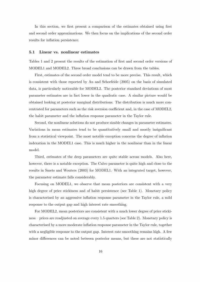
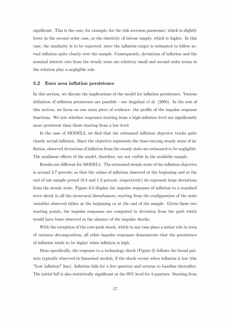
In this section, we first present a comparison of the estimates obtained using first

and second order approximations. We then focus on the implications of the second order

results for inflation persistence.

5.1 Linear vs. nonlinear estimates

Tables 1 and 2 present the results of the estimation of first and second order versions of

MODEL1 and MODEL2. Three broad conclusions can be drawn from the tables.

First, estimates of the second order model tend to be more precise. This result, which

is consistent with those reported by An and Schorfeide (2005) on the basis of simulated

data, is particularly noticeable for MODEL2. The posterior standard deviations of most

parameter estimates are in fact lower in the quadratic case. A similar picture would be

obtained looking at posterior marginal distributions. The distribution is much more con-

centrated for parameters such as the risk aversion coefficient and, in the case of MODEL2,

the habit parameter and the inflation response parameter in the Taylor rule.

Second, the nonlinear solutions do not produce sizable changes in parameter estimates.

Variations in mean estimates tend to be quantitatively small and mostly insignificant

from a statistical viewpoint. The most notable exception concerns the degree of inflation

indexation in the MODEL1 case. This is much higher in the nonlinear than in the linear

model.

Third, estimates of the deep parameters are quite stable across models. Also here,

however, there is a notable exception. The Calvo parameter is quite high and close to the

results in Smets and Wouters (2003) for MODEL1. With an integrated target, however,

the parameter estimate falls considerably.

Focusing on MODEL1, we observe that mean posteriors are consistent with a very

high degree of price stickiness and of habit persistence (see Table 1). Monetary policy

is characterised by an aggressive inflation response parameter in the Taylor rule, a mild

response to the output gap and high interest rate smoothing.

For MODEL2, mean posteriors are consistent with a much lower degree of price sticki-

ness — prices are readjusted on average every 1.5 quarters (see Table 2). Monetary policy is

characterised by a more moderate inflation response parameter in the Taylor rule, together

with a negligible response to the output gap. Interest rate smoothing remains high. A few

minor differences can be noted between posterior means, but these are not statistically

16

significant. This is the case, for example, for the risk aversion paratemer, which is slightly

lower in the second order case, or the elasticity of labour supply, which is higher. In this

case, the similarity is to be expected, since the inflation target is estimated to follow ac-

tual inflation quite closely over the sample. Consequently, deviations of inflation and the

nominal interest rate from the steady state are relativey small and second order terms in

the solution play a negligible role.

5.2 Euro area inflation persistence

In this section, we discuss the implications of the model for inflation persistence. Various

definition of inflation persistence are possible — see Angeloni et al. (2005). In the rest of

this section, we focus on one main piece of evidence: the profile of the impulse response

functions. We test whether responses starting from a high-inflation level are significantly

more persistent than those starting from a low level.

In the case of MODEL2, we find that the estimated inflation objective tracks quite

closely actual inflation. Since the objective represents the time-varying steady state of in-

flation, observed deviations of inflation from the steady state are estimated to be negligible.

The nonlinear effects of the model, therefore, are not visible in the available sample.

Results are different for MODEL1. The estimated steady state of the inflation objective

is around 2.7 percent, so that the values of inflation observed at the beginning and at the

end of our sample period (9.4 and 1.2 percent, respectively) do represent large deviations

from the steady state. Figure 2-5 display the impulse responses of inflation to a standard

error shock in all the structural disturbances, starting from the configuration of the state

variables observed either at the beginning or at the end of the sample. Given these two

starting points, the impulse responses are computed in deviation from the path which

would have been observed in the absence of the impulse shocks.

With the exception of the cost-push shock, which in any case plays a minor role in term

of variance decomposition, all other impulse responses demonstrate that the persistence

of inflation tends to be higher when inflation is high.

More specifically, the response to a technology shock (Figure 2) follows the broad pat-

tern typically observed in linearised models, if the shock occurs when inflation is low (the

"Low inflation" line). Inflation falls for a few quarters and returns to baseline thereafter.

The initial fall is also statistically significant at the 95% level for 4 quarters. Starting from

17

a high inflation level (the "High inflation" line) however, the fall in inflation is reduced

dramatically and ceases to be significant from a statistical viewpoint. In addition, the

median response tends to have a much more persistent effects. Ten years after the shock,

inflation remains around the level observed on impact.

The response to a positive inflation target shocks is even more starkly different de-

pending on the starting point (Figure 3). The response is very similar to the linear case,

if the shock hits when inflation is low. If inflation is already high, however, it tends to rise

further on impact, after the shock, and to build up considerably thereafter (before being

eventually reabsorbed). From a quantitative viewpoint, the impact of a given target shock

is almost twice as big, and the difference is almost always significant from a statistical

viewpoint. Nevertheless, in terms of persistence profile, the shock has similar effects inde-

pendently of the starting point: inflation peaks after approximately 2 years and remains

close to this higher level for the remaining 8 years displayed in the figure.

Finally, some quantitative differences between median responses are noticeable also

in the cost-push and policy shock cases (Figures 4 and 5, respectively). However, these

responses tend to be insignificant from a statistical viewpoint. More specifically, the

cost-push shock has a truly negligible impact on inflation dynamics. As to the policy

shock, after a surprising interest rate hike the median fall in inflation is smaller, when

the starting point is a high inflation level. This would imply that "surprise" disinflations

become increasingly costly the higher the level inflation is allowed to reach.

6 Conclusions

Our preliminary results suggest that the nonlinearities in the dynamics of inflation can

have pronounced and statistically significant effects at some points in time. From a more

general viewpoint, our results illustrate some of the main advantages and disadvantages

of estimating DSGE models based on a nonlinear approximation.

Advantages

1. Increase in the identifiability of parameters. Recent literature (eg. Canova and Sala,

2005) has emphasised the chronic under-identification of many DSGE models. It is

possible to verify that resorting to higher order approximation induces sensibly more

curvature in the likelihood function hence increases identifiability of the parameters.

18

We have verified this feature also for the models that we estimate in this paper,

both on the real dataset and on simulated data. An interesting qualification of this

identification-enhancing feature of non-linear approximation is that it is very evident

for those parameters for which the likelihood has some (even minimal) curvature

already with the linear solution. If the likelihood is absolutely flat in the linear

case, it tends to remain flat. We believe that this increase of likelihood curvature is

generated by the fact that the nonlinear approximation generates many relationships

involving first and second order moments of the distribution for the data.

2. Theoretical importance of higher order terms. In many applications the higher order

terms of the solution of a DSGE model cannot be neglected. In particular, when a

DSGE model is used for asset pricing, the linear approximation by definition is not

capable of delivering correct prescriptions.

3. Accuracy of likelihood computations. The recent literature (Fernandez-Villaverde et

al. 2005) point out that a linear approximation to the solution of a DSGE model,

induces cumulation of errors in the evaluation of the likelihood. Therefore likelihood

based inference based on the linear approximation can be misleading.

4. More flexibility in model specification. Many different interesting features can be

easily accommodated in a very flexible way. It is possible to assume stochastic volatil-

ity, Markov switching (in this way accommodating highly needed time heterogeneity

of the data generation mechanism), GARCH effects etc...

5. It is also worth pointing out that the use of SMC techniques can be very useful

also in models which can be estimated using usual filtering techniques but situations

in which recursive Bayesian estimation is required, for example in order to assess

pseudo out of sample forecasting performance. In such cases variants of the PF could

be easily and profitably used.

Disadvantages

1. Computation time. The first disadvantage of using non linear approximations (and

the simulation filtering that is necessary to carry out likelihood based inference) is

essentially that much more computation time is required. This is clearly not very

nice, since Bayesian estimation of DSGE models typically requires running multiple,

19

long chains after having tuned carefully (and painfully through the use of many

chains) the candidate distribution for the parameters. The methodological "silver

lining" of this feature is that the researcher can do data mining only with geological

endowments of time.

2. Frequent occurrence of numerical problems. We have experienced a strong sensitivity

of SMC methods to outliers and degeneracies which frequently arise in actual data.

The researcher has to be very careful in monitoring the numerical efficiency indicators

of the filter that is being used. Moreover the non linear state space system that

arises often implies explosive behaviour for the state variables also for parameter

values which would assign a stationary distribution to the state variables in a linear

setting. Great care has to be to put in designing a prior distribution that rules out

such occurrences.

20

Table 1: Estimation results: MODEL1

I order approx II order approxprior mean prior sd post mean post sd post mean post sd

γ 2.000 0.705 2.233 0.728 1.139 0.087h 0.699 0.138 0.736 0.069 0.799 0.071φ 3.982 1.993 5.265 2.091 2.290 0.899θ 7.985 2.648 9.188 2.807 6.996 2.058ζ 0.602 0.147 0.855 0.049 0.898 0.072ι 0.666 0.179 0.304 0.157 0.771 0.111ψπ 0.500 0.092 0.445 0.085 0.332 0.061ψy 0.050 0.035 0.017 0.012 0.045 0.025ρi 0.799 0.100 0.925 0.041 0.913 0.056ρτ 0.500 0.151 0.498 0.152 0.515 0.100ρa 0.901 0.090 0.990 0.007 0.994 0.004ρπ 0.898 0.093 0.992 0.004 0.995 0.003στ 0.040 0.013 0.040 0.013 0.035 0.011σa 0.003 0.001 0.009 0.002 0.008 0.001σπ 0.001 0.001 0.001 2.E-04 0.001 3.E-04σi 0.001 3.E-04 0.002 1.E-04 0.002 1.E-04τ 0.398 0.284 2.E-04 1.E-04 3.E-04 1.E-04π 1.005 0.003 1.005 0.003 1.007 0.003

σm,π 0.010 0.014 0.003 4.E-04 0.003 0.001σm,i 0.010 0.014 0.011 0.014 1.E-07 1.E-07σm,y 0.010 0.014 0.010 0.014 0.021 0.015

Note: σd = 0, α = 0.76, χ = 0.275, β = 0.9944.

21

Table 2: Estimation results: MODEL2

I order approx II order approxprior mean prior sd post mean post sd post mean post sd

β 0.902 0.091 0.992 0.001 0.991 0.001γ 2.000 0.708 2.064 0.737 1.469 0.055h 0.700 0.139 0.632 0.104 0.721 0.029φ 4.979 1.965 2.798 0.880 4.856 0.590θ 7.996 2.646 6.991 2.288 7.514 1.737ζ 0.601 0.146 0.404 0.093 0.312 0.080ψπ 1.502 0.352 1.524 0.289 1.556 0.078ψy 0.050 0.035 0.053 0.035 0.035 0.008ρi 0.701 0.137 0.947 0.020 0.926 0.021ρτ 0.500 0.151 0.213 0.096 0.448 0.031ρa 0.901 0.089 0.997 0.003 0.981 0.004στ 0.040 0.040 0.165 0.074 0.037 0.006σa 0.003 0.005 0.011 0.003 0.011 0.001σπ 0.001 0.001 2.E-04 3.E-04 0.001 3.E-04σi 0.001 0.002 0.001 2.E-04 0.001 4.E-04τ 0.401 0.286 0.792 0.353 0.122 0.019

σm,π 0.010 0.014 1.E-03 1.E-04 0.001 0.001σm,i 0.010 0.014 4.E-05 6.E-05 0.001 3.E-04σm,y 0.010 0.014 0.002 5.E-04 0.002 4.E-04

Note: σd = 0, α = 0.76, χ = 0.275, ι = 1.0.

22

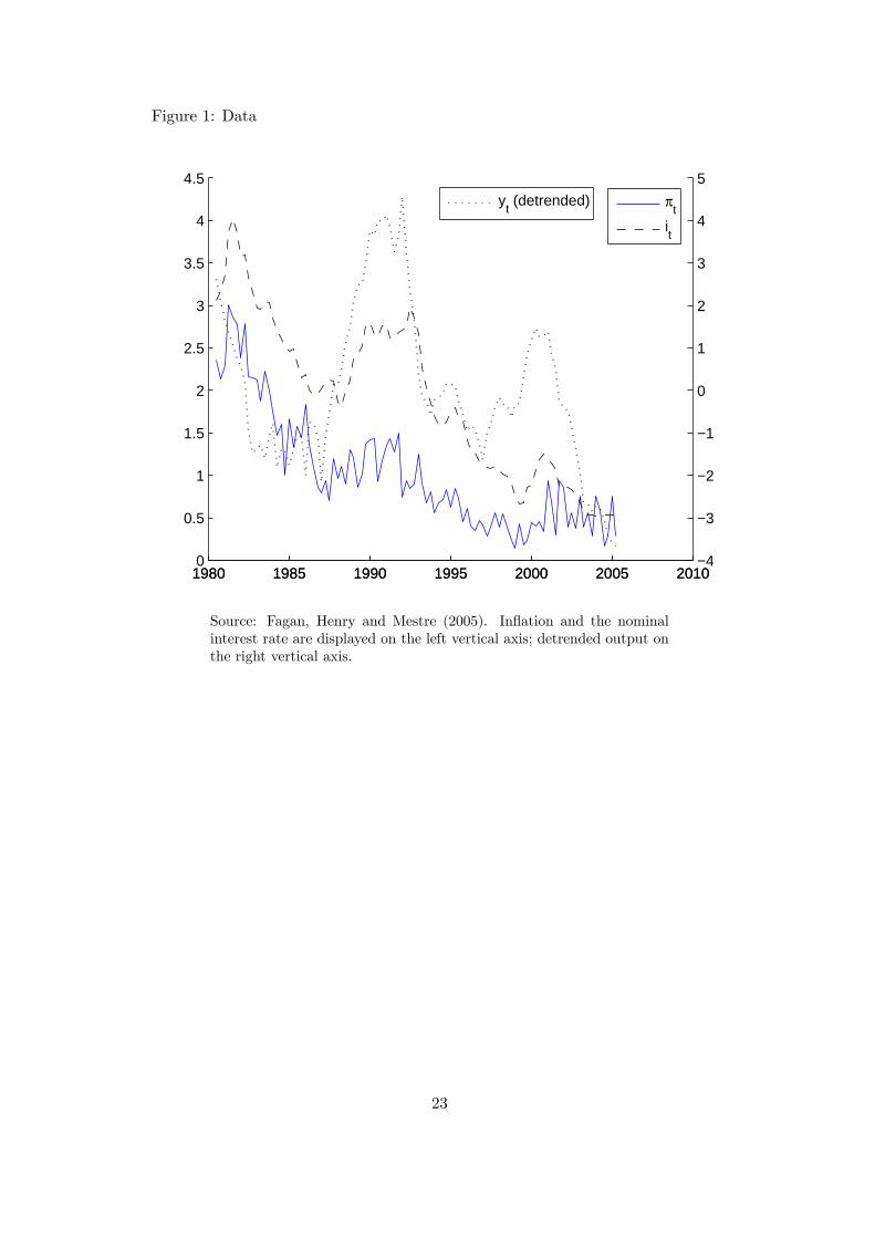
Figure 1: Data

1980 1985 1990 1995 2000 2005 20100

0.5

1

1.5

2

2.5

3

3.5

4

4.5

1980 1985 1990 1995 2000 2005 2010−4

−3

−2

−1

0

1

2

3

4

5

yt (detrended) π

t

it

Source: Fagan, Henry and Mestre (2005). Inflation and the nominalinterest rate are displayed on the left vertical axis; detrended output onthe right vertical axis.

23

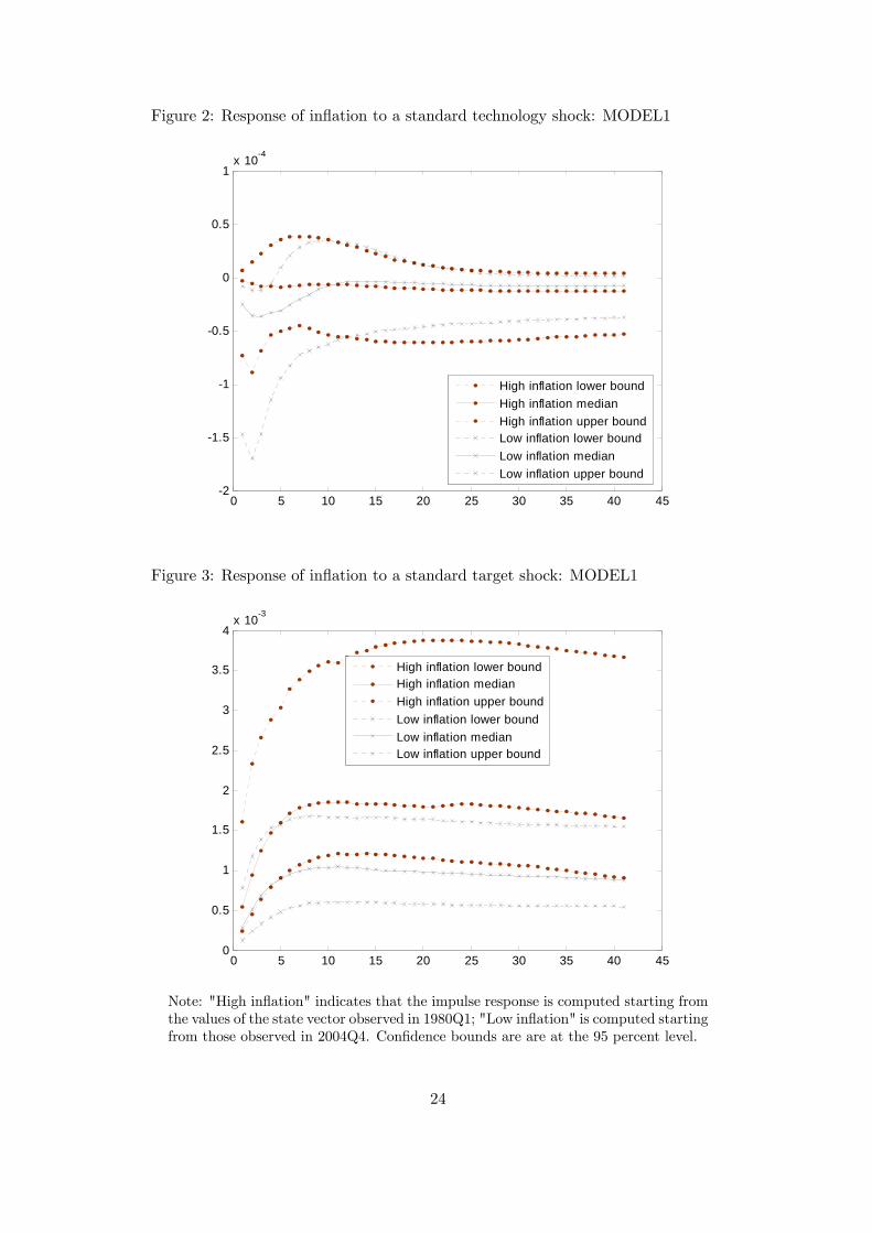
Figure 2: Response of inflation to a standard technology shock: MODEL1

0 5 10 15 20 25 30 35 40 45-2

-1.5

-1

-0.5

0

0.5

1x 10-4

High inflation lower boundHigh inflation medianHigh inflation upper boundLow inflation lower boundLow inflation medianLow inflation upper bound

Figure 3: Response of inflation to a standard target shock: MODEL1

0 5 10 15 20 25 30 35 40 450

0.5

1

1.5

2

2.5

3

3.5

4x 10-3

High inflation lower boundHigh inflation medianHigh inflation upper boundLow inflation lower boundLow inflation medianLow inflation upper bound

Note: "High inflation" indicates that the impulse response is computed starting fromthe values of the state vector observed in 1980Q1; "Low inflation" is computed startingfrom those observed in 2004Q4. Confidence bounds are are at the 95 percent level.

24

Figure 4: Response of inflation to a standard cost-push shock: MODEL1

0 5 10 15 20 25 30 35 40 45-2

0

2

4

6

8

10

12x 10-8

High inflation lower boundHigh inflation medianHigh inflation upper boundLow inflation lower boundLow inflation medianLow inflation upper bound

Figure 5: Response of inflation to a standard policy shock: MODEL1

0 5 10 15 20 25 30 35 40 45-6

-5

-4

-3

-2

-1

0

1

2x 10-4

High inflation lower boundHigh inflation medianHigh inflation upper boundLow inflation lower boundLow inflation medianend sample upper bound

Note: "High inflation" indicates that the impulse response is computed starting fromthe values of the state vector observed in 1980Q1; "Low inflation" is computed startingfrom those observed in 2004Q4. Confidence bounds are are at the 95 percent level.

25

A Appendix

[To be written]

References

[1] An and Schorfeide (2005), “Bayesian analysis of DSGE models”

[2] Angeloni et al. (2005)

[3] Arulampalam et al. (2002),

[4] Aruoba, Fernandez-Villaverde and Rubio-Ramirez (2003), “Comparing Solution

Methods for Dynamic Equilibrium Economies”

[5] Ascari, G. (2004), “Staggered Prices and Trend Inflation: Some Nuisances,” Review

of Economic Dynamics 7, 642-667.

[6] Bilke (2004)

[7] Calvo, G. A. (1983), “Staggered prices in a utility-maximising framework,” Journal

of Monetary Economics 12, 983-98.

[8] Canova, F. and L. Sala (2005), “Back to square one: identification issues in DSGE

models,” mimeo, June.

[9] Chib (2001),

[10] Christiano, L., M. Eichenbaum and C. L. Evans, (2005), “Nominal Rigidities and the

Dynamic Effects of a Shock to Monetary Policy,” Journal of Political Economy 113,

1-45.

[11] Clarida, R., J. Galí and M. Gertler, 1998, Monetary policy rules in practice: Some

international evidence, European Economic Review, 42, 1033-1067.

[12] Clarida, R., J. Galí and M. Gertler (2000), “Monetary Policy Rules and Macro-

economic Stability: Evidence and Some Theory,” Quarterly Journal of Economics,

147-180.

[13] Corvoisier and Mojon (2004)

26

[14] Dossche and Everaert (2004)

[15] Doucet, A., N. de Freitas and N. Gordon (2001), eds., Sequential Monte Carlo Meth-

ods in Practice, New York: Springer-Verlag.

[16] Fagan, G., J. Henry and R. Mestre (2005), “An area-wide model (AWM) for the euro

area,” Economic Modelling 22, 39-59.

[17] Fernandez-Villaverde and Rubio-Ramirez (2004), “Estimating macroeconomic mod-

els: a likelihood approach,”

[18] Fernandez-Villaverde, Rubio-Ramirez and Santos (2005), “Convergence properties of

the likelihood of computed dynamic models,”

[19] Geweke and McCausland (2002),

[20] Hamilton, J. (1994), Time series analysis, (Princeton University Press, Princeton).

[21] Hördahl, P., O. Tristani and D. Vestin (2005), “A joint econometric model of macro-

economic and term structure dynamics,” Journal of Econometrics, forthcoming.

[22] Kim, J., S. Kim, E. Schaumburg and C. Sims (2003), “Calculating and using sec-

ond order accurate solutions of discrete time dynamic equilibrium models”, mimeo,

August.

[23] Klein, Paul (2005), “Second-order approximation of dynamic models without the use

of tensors,” University of Western Ontario, mimeo, August.

[24] Levin and Piger (2004)

[25] Liu and West (2001),

[26] Schmitt-Grohé and Uribe (2004), “Solving dynamic general equilibrium models using

a second-order approximation to the policy function,” Journal of Economic Dynamics

and Control 28, 755-75.

[27] Schorfeide, F. (2005), “Learning and Monetary Policy Shifts,” Review of Economic

Dynamics 8, 392-419.

[28] Smets, F. and R. Wouters (2003), “An estimated stochastic dynamic general equilib-

rium model of the euro area,” Journal of European Economic Association 1, 1123-75

27

[29] Smets, F. and R. Wouters (2005), “Comparing shocks and frictions in US and euro

area business cycles: a Bayesian DSGE approach,” Journal of Applied Econometrics

20, forthcoming.

[30] Steinsson (2003)

[31] Sutherland, A. (2002), “A simple second-order solution method for dynamic general

equilibrium models,” CEPR Discussion Paper No. 3554.

[32] Woodford, M. (2003), Interest and Prices, Princeton University Press.

[33] Yun (1996)

28