arX

iv:c

ond-

mat

/040

1438

v2 [

cond

-mat

.sta

t-m

ech]

15

Jun

2004

Persistence in nonequilibrium surface growth

M. Constantin,1, 2 C. Dasgupta,1, 3 P. Punyindu Chatraphorn,1, 4 Satya N. Majumdar,5, 6 and S. Das Sarma1

1 Condensed Matter Theory Center, Department of Physics,

University of Maryland, College Park, Maryland 20742-4111, USA2Materials Research Science and Engineering Center, Department of Physics,

University of Maryland, College Park, Maryland 20742-4111, USA3Department of Physics, Indian Institute of Science, Bangalore 560012, India

4 Department of Physics, Faculty of Science, Chulalongkorn University, Bangkok, Thailand5Laboratoire de Physique Quantique, UMR C5626,

Universite Paul Sabatier, 31062 Toulouse Cedex, France6Laboratoire de Physique Theorique et Modeles Statistiques,

Universite Paris-Sud, Bat. 100, 91405 ORSAY Cedex, France

Persistence probabilities of the interface height in (1+1)– and (2+1)–dimensional atomistic, solid–on–solid, stochastic models of surface growth are studied using kinetic Monte Carlo simulations, withemphasis on models that belong to the molecular beam epitaxy (MBE) universality class. Both theinitial transient and the long–time steady–state regimes are investigated. We show that for growthmodels in the MBE universality class, the nonlinearity of the underlying dynamical equation isclearly reflected in the difference between the measured values of the positive and negative persistenceexponents in both transient and steady–state regimes. For the MBE universality class, the positiveand negative persistence exponents in the steady–state are found to be θS

+ = 0.66 ± 0.02 and θS− =

0.78±0.02, respectively, in (1+1) dimensions, and θS+ = 0.76±0.02 and θS

− = 0.85±0.02, respectively,in (2+1) dimensions. The noise reduction technique is applied on some of the (1+1)–dimensionalmodels in order to obtain accurate values of the persistence exponents. We show analytically thata relation between the steady–state persistence exponent and the dynamic growth exponent, foundearlier to be valid for linear models, should be satisfied by the smaller of the two steady-statepersistence exponents in the nonlinear models. Our numerical results for the persistence exponentsare consistent with this prediction. We also find that the steady–state persistence exponents can beobtained from simulations over times that are much shorter than that required for the interface toreach the steady state. The dependence of the persistence probability on the system size and thesampling time is shown to be described by a simple scaling form.

PACS numbers: 81.10.Aj, 05.20.-y, 05.40.-a, 68.35.Ja

I. INTRODUCTION

Nonequilibrium surface growth and interface dynamics represent an area of research that has received much atten-tion in the last two decades [1]. A large number of discrete atomistic growth models [2, 3, 4, 5, 6, 7, 8] and stochasticgrowth equations [9, 10, 11, 12, 13, 14] have been found [15] to exhibit generic scale invariance characterized by powerlaw behavior of several quantities of interest, such as the interface width as a function of time (measured in units ofdeposited layers) and space- and time–dependent correlation functions of the interface height. Much effort has beendevoted to the classification of growth models and equations into different universality classes characterized by thevalues of the exponents that describe the dynamic scaling behavior implied by these power laws. A variety of experi-mental studies [15, 16] have confirmed the occurrence of dynamic scaling in nonequilibrium epitaxial growth. Amongthe various experimental methods of surface growth, molecular beam epitaxy (MBE) is especially important becauseit plays a crucial role in the fabrication of smooth semiconductor films required in technological applications. Underusual MBE growth conditions, desorption from the film surface is negligible and the formation of bulk vacancies andoverhangs is strongly suppressed. It is generally believed that nonequilibrium surface growth under these conditions iswell–described by a conserved nonlinear Langevin–type equation [12, 13, 14] and related atomistic models [3, 5, 8, 14]that form the so–called “MBE universality class”.

Surface growth is an example of a general class of problems involving the dynamics of non–Markovian, spatiallyextended, stochastic systems. In recent years, the concept of persistence [17] has proven to be very useful in analyzingthe dynamical behavior of such systems [18, 19, 20, 21, 22, 23, 24]. Loosely speaking, a stochastic variable is persistent

if it has a tendency to maintain its initial characteristics over a long period of time. The persistence probability P (t)is typically defined as the probability that a characteristic feature (e.g. the sign) of a stochastic variable does notchange at all over a certain period of time t. Although the mathematical concept of persistence was introduced along time ago in the context of the “zero–crossing problem” in Gaussian stationary processes [25], it is only veryrecently that this concept has received attention in describing the statistics of first passage events in a variety ofspatially extended nonequilibrium systems. Examples of such applications of the concept of persistence range from

2

the fundamental classical diffusion equation [18] to the zero temperature Glauber dynamics of the ferromagnetic Isingand q–state Potts models [19, 20, 21, 26] and phase ordering kinetics [22]. Recently, a generalization of the persistenceconcept (probability of persistent large deviations) has been introduced [26]. A closely related idea, that of sign–timedistribution, was developed in Ref. [27]. An increasing number of experimental results are also available for persistencein systems such as coalescence of droplets [28], coarsening of two–dimensional soap froth [29], twisted nematic liquidcrystal [30], and nuclear spin distribution in laser polarized Xe129 gas [31].

Recent work of Krug and collaborators [23, 24] has extended the persistence concept to the first–passage statisticsof fluctuating interfaces. Persistence in the dynamics of fluctuating interfaces is of crucial importance in ultra–smallscale solid–state devices. As the technology advances into the nanometric regime, questions such as how long aparticular perturbation that appears in an evolving interface persists in time and what is the average time requiredfor a structure to first fluctuate into an unstable configuration become important. The persistence probability canprovide quantitative predictions on such questions. Recent experiments [32, 33, 34] have demonstrated the usefulnessof the concept of persistence in the characterization of the equilibrium fluctuations of steps on a vicinal surface.Analysis of experimental data on step fluctuations on Al/Si(111) [32, 34] and Ag(111) [33, 34] surfaces has shownthat the long–time behavior of the persistence probability and the probability of persistent large deviations in thesesystems agrees quantitatively with the corresponding theoretical predictions. These results show that the persistenceprobability and related quantities are particularly relevant for describing and understanding the long–time dynamicsof interface fluctuations.

In the context of surface growth and fluctuations, the persistence probability P (t0, t0 + t) may be defined as theprobability that starting from an initial time t0, the interfacial height h(r, t′) at spatial position r does not returnto its original value at any point in the time interval between t0 and t0 + t. This probability is clearly the sum ofthe probabilities of the height h(r, t′) always remaining above (the positive persistence probability P+) and alwaysremaining below (the negative persistence probability P−) its specific initial value h(r, t0) for all t0 < t′ ≤ t0 + t. Thisconcept quantifies the tendency of a stochastic field (in our case the interface height) to persistently conserve a specificfeature (the sign of the interfacial height fluctuations). The persistence probability P (t0, t0 + t) would, in general,depend on both t0 and t. In the early stage of the growth process starting from a flat interface (transient regime), theinterface gradually develops dynamical roughness [1] due to the effect of fluctuations in the beam intensity. In thisregime, the choice of the initial time t0 is clearly important: it determines the degree of roughness of the configurationfrom which the interface evolves. At long times, the growing interface enters into a new evolution stage, called thesteady–state regime, characterized by fully developed roughness that does not increase further in time. In this regime,the choice of t0 is expected to be unimportant.

The work of Krug et al. [23] shows that for a class of linear Langevin–type equations for surface growth and atomisticmodels belonging in the same dynamical universality class as these equations, the persistence probability decays asa power law in time for long times in both transient and steady–state regimes. These power laws define the positiveand negative persistence exponents, θT

± and θS±, for positive and negative persistence in the transient and steady–state

regimes, respectively. The h → −h symmetry of the linear growth equations implies that θT+ = θT

− and θS+ = θS

− inthese systems. In Ref. 23, it was pointed out that the persistence exponent in the steady state of these linear modelsis related to the dynamic scaling exponent β, that describes the growth of the interface width W as a function of timet in the transient regime (W ∝ tβ), through the relation θS

+ = θS− = 1−β. The validity of this relation was confirmed

by numerical simulations. Since the exponent β is the same for all models in the same dynamical universality class,this result implies that the persistence exponent in the steady–state regime of these linear models is also universal.Numerical results for the persistence exponent in the transient regime, for which no analytic predictions are available,also indicate a similar universality. Kallabis and Krug [24] carried out a similar calculation for (1+1)–dimensionalKardar–Parisi–Zhang (KPZ) [11] interfaces. They found that the nonlinearity in the KPZ equation that breaks theh → −h symmetry is reflected in different values of the positive and negative persistence exponents, θT

+ and θT−, in the

transient regime. The values of the steady–state persistence exponents θS+ and θS

− were found to be equal to each other,and equal to 1 − β within the accuracy of the numerical results. This is expected because the h → −h symmetry isdynamically restored in the steady state of the (1+1)–dimensional KPZ equation. This is, however, a specific featureof the (1+1)–dimensional KPZ model, which for nongeneric reasons, turns out to be up–down symmetric in the steadystate. Nonlinear surface growth models (e.g. the higher dimensional KPZ model, the nonlinear MBE growth model)are generically expected to have different values of θ± in both transient and steady–state regimes.

In this paper, we present the results of a detailed numerical study of the persistence behavior of several atomistic,solid–on–solid (SOS) models of surface growth in (1+1) and (2+1) dimensions. While we concentrate on modelsin the MBE universality class, results for a few other models, some of which have been studied in Refs. 23 and24 are also presented for completeness. The highly non–trivial nature of the persistence probability, in spite of adeceptive simplicity of the defining concept, arises from the complex temporal non–locality (“memory”) inherentin its definition. In fact, there are very few stochastic problems where an analytical solution for the persistenceprobability has been achieved. These include the classical Brownian motion [35], the random acceleration problem

3

[36] and the one dimensional Ising and q-state Potts models [20]. In general, the highly nonlocal nature of thetemporal correlations in a non–Markovian stochastic process makes it extremely difficult to obtain exact results forthe persistence probability even for seemingly simple stochastic processes. Even for the simple diffusion equation,the persistence exponent is known only numerically, or within an independent interval approximation [18] or seriesexpansion approach [37]. However, it is fairly straightforward in most cases to directly simulate the persistenceprobability to obtain its stationary power law behavior at large times, and thus to numerically obtain the approximatevalue of the persistence exponent. For this reason, we use stochastic (Monte Carlo) simulations of the atomistic growthmodels to study their temporal persistence behavior in the transient and steady–state regimes. These models aredefined in terms of random deposition and specific cellular–automaton–type local diffusion or relaxation rules. Someof these models are of the “limited–mobility” type in the sense that the surface diffusion rules or local restrictions limitthe characteristic length over which a deposited particle can diffuse to just one or a few lattice spacings. The modelsin the MBE universality class considered in our study are: the Das Sarma–Tamborenea model [3], the Wolf–Villainmodel [4, 38], the Kim–Das Sarma model [5] and its “controlled” version [14], and the restricted solid–on–solid(RSOS) model of Kim at al. [8]. We also present results for the Family model [2] that is known to belong to theEdwards–Wilkinson [10] universality class and the restricted solid–on–solid (RSOS) model of Kim and Kosterlitz [7]that is in the KPZ universality class.

The main objective of our study is to examine the effects of the nonlinearity in the MBE growth equation [12, 13] onthe persistence behavior. Unlike the (1+1)–dimensional KPZ equation, the nonlinearity in the MBE growth equationpersists in the steady state in the sense that the height profile exhibits a clear asymmetry between the positive andnegative directions (above and below the average height). Therefore, the positive and negative persistence exponentsθS+ and θS

− are expected to have different values in these models. If this is the case, then the relation between thesteady–state persistence exponent and the dynamic scaling exponent β found in linear models can not be valid forboth θS

+ and θS−, indicating that at least one of these exponents is a new, nontrivial one not related to the usual

dynamic scaling exponents. The values of θS+ and θS

− and their relation to β, as well as the values of the transient

persistence exponents θT+ and θT

− are the primary questions addressed in our study. We also investigate the universalityof these exponents by measuring them for several models that are known to belong in the same universality class asfar as their dynamic scaling behavior is concerned. To obtain accurate values of the exponents, the “noise reduction”technique [39] is employed in some of the simulations of (1+1)–dimensional models. We also address some questionsrelated to the methodology of calculating persistence exponents from simulations. Since the value of the dynamicalexponent z is relatively large for models in the MBE universality class, the time required for reaching the steady stategrows quickly as the sample size L is increased (tsat ∝ Lz). As a result, it is difficult to reach the steady state insimulations for large L. It is, therefore, useful to find out whether the value of the steady–state persistence exponentscan be extracted from calculations of P (t0, t0 + t) with t0 ≪ tsat ∝ Lz. Another issue in this context involves theeffects of the finiteness of the sample size L and the sampling time δt (the time interval between two successivemeasurements of the height profile) on the calculated persistence probability. An understanding of these effects isneeded for extracting reliable values of the persistence exponents from simulations that always involve finite values ofL and δt. Understanding the effects of L and δt on the persistence analysis is not only important for our simulations,but is also important in the experimental measurements of persistence which invariably involve finite system size andsampling time.

The main results of our study are as follows. We find that the positive and negative steady–state persistence expo-nents for growth models in the MBE universality class are indeed different from each other, reflecting the asymmetryof the interface arising from the presence of nonlinearities in the underlying growth equation. Our results for theseexponent values are: θS

+ = 0.66 ± 0.02 and θS− = 0.78 ± 0.02, respectively, in (1+1) dimensions; θS

+ = 0.76 ± 0.02 and

θS− = 0.85 ± 0.02 in (2+1) dimensions. The values of the positive and negative persistence exponents for different

models are clearly correlated with the asymmetry of the “above” and ”below” (defined relative to the mean interfaceheight) portions of the interface. We show analytically that the smaller one of the two steady-state persistence expo-nents should be equal to (1 − β). Thus, the relation θ = 1 − β derived in Ref. [23] for linear surface growth modelsis expected to be satisfied by θS

+ for the nonlinear models considered here. Our numerical results are consistent withthis expectation: we find that the positive persistence exponent is indeed close to (1 − β), while the negative one issignificantly higher. Similar asymmetry is found for the persistence exponents in the transient regime with θT

+ < θT−

in MBE growth. Within the uncertainties in the numerically determined values of the exponents, they are universalin the sense that different models in the same dynamic universality class yield very similar values for these exponents.For the models in the Edwards–Wilkinson and KPZ universality classes, we find results in agreement with those ofearlier studies [23, 24].

Our simulations also reveal that a measurement of the steady–state persistence exponents is possible from simu-lations in which the initial time t0 is much smaller than the time (∼ Lz) required for the interfacial roughness tosaturate. A similar result was reported in Ref. 23 where it was found that the steady–state persistence exponent maybe obtained from a calculation of P (t0, t0 + t) with t ≪ t0 ≪ Lz. We find that the restriction t ≪ t0 is not necessary

4

for seeing a power law behavior of P±(t0, t0 + t) – a power law with the steady–state exponents is found even if tis close to or somewhat larger than t0. We exploit this finding in some of our persistence simulations for (2+1)–dimensional growth models which are more relevant to experiments. These results, however, also imply that it wouldbe extremely difficult to measure the transient persistence exponents from real surface growth experiments. Finally,we show that the dependence of the steady–state persistence probability on the sample size L and the sampling timeδt is described by a simple scaling function of the variables t/Lz and δt/Lz. This scaling description is similar to thatfound recently [40] for a different “persistence probability”, the survival probability, that measures the probability ofthe height not returning to its average value (rather than the initial value) over a certain period of time. Althoughthe “persistence” and the “survival” [40] probability seem to be qualitatively similar in their definitions, the two aremathematically quite unrelated, and in fact, no exponent can be defined for the survival probability. In this paperwe only discuss the persistence probability and the persistence exponent for surface growth processes.

The rest of the paper is organized as follows: in Sec. II A, we briefly discuss the main universality classes and theircorresponding dynamic equations and scaling exponents relevant for surface growth phenomena. Section II B containsa short overview of the persistence probability concept from the interface fluctuations perspective. The discretestochastic SOS growth models considered in our study are described in Sec. III. In addition, we briefly describein this section the noise reduction technique which is employed in some of our simulations. Section IV contains adetailed description of our main results: in Sec. IVA, our (1+1)–dimensional simulation results for the transientand steady–state persistence exponents are presented, focusing mostly on models described by the nonlinear MBEdynamical equation. Section IVB contains the analytic derivation of a relation between the smaller steady-statepersistence exponent and the dynamic growth exponent. In Sec. IVC, we introduce an alternative approach formeasuring the steady–state persistence exponents, using a relatively short “equilibration time” that is much shorterthan the time required for reaching the true steady state. Section IVD contains the results of our (2+1)–dimensionalpersistence calculation for a selection of linear and nonlinear models. Simulation results that establish a scaling formof the dependence of the persistence probability on the sample size and the sampling time are presented in Sec. IV E.The final Sec. V contains a summary of our main results and a few concluding remarks.

II. STOCHASTIC GROWTH EQUATIONS AND PERSISTENCE PROBABILITIES

A. Growth equations and dynamic scaling

The dynamic scaling behavior of stochastic growth equations may be classified into several universality classes. Eachuniversality class is characterized by a set of scaling exponents [1] which depend on the dimensionality of the problem.These exponents are (α, β, z), where α is the roughness exponent describing the dependence of the amplitude of heightfluctuations in the steady–state regime (t ≫ Lz) on the sample size L, β is the growth exponent that describes theinitial power law growth of the interface width in the transient regime (1 ≪ t ≪ Lz), and z is the dynamical exponentrelated to the system size dependence of the time at which the interface width reaches saturation. Note that z = α

β

for all the models considered in this paper. To describe the interface evolution we use the single–valued function,h(r, t), which represents the height of the growing sample at position r and deposition time t. The interfacial heightfluctuations are described by the root–mean–squared height deviation (or interface width) which is a function of thesubstrate size L and deposition time t:

W (L, t) = 〈(h(r, t) − h̄(t))2〉1/2, (1)

where h̄(t) is the average sample thickness. The width W (L, t) scales as W (L, t) ∝ tβ for t ≪ Lz and W (L, t) ∝ Lα

for t ≫ Lz [41], Lz being the equilibration time of the interface, when its stationary roughness is fully developed.Since it is convenient to write the evolution equations in terms of the deviation of the height from its spatial average

value, h(r, t)− h̄(t), from now on we will denote by h(r, t) the interface height fluctuation measured from the averageheight. Extensive studies of dynamic scaling in kinetic surface roughening (for an extended review see Ref. [15]) haverevealed the existence of (at least) four universality classes that are described, in the long wavelength limit, by thefollowing continuum equations and sets of scaling exponents (α, β, z), shown for the 1+1(2+1)–dimensional cases,respectively:(1) The Edwards–Wilkinson (EW) second order linear equation: 1

2, 1

4, 2 (0 (log), 0 (log), 2)

∂h(r, t)

∂t= ν2∇

2h(r, t) + η(r, t), (2)

(2) The KPZ second order nonlinear equation: 12, 1

3, 3

2(≃ 0.4, ≃ 0.24, ≃ 1.67)

∂h(r, t)

∂t= ν2∇

2h(r, t) + λ2|∇h(r, t)|2 + η(r, t), (3)

5

(3) The Mullins–Herring (MH) fourth order linear equation: 32, 3

8, 4 (1, 1

4, 4)

∂h(r, t)

∂t= −ν4∇

4h(r, t) + η(r, t), (4)

and(4) The MBE fourth order nonlinear equation: ≃ 1, ≃ 1

3, ≃ 3 (≃ 2

3, ≃ 1

5, ≃ 10

3)

∂h(r, t)

∂t= −ν4∇

4h(r, t) + λ22∇2|(∇h(r, t)|2 + η(r, t), (5)

where νi (i=2, 4) and λj (j=2, 22) are constant. The quantity η(r, t) represents the noise term which accounts forthe random fluctuations in the deposition rate. We assume that the noise has Gaussian distribution with zero meanand correlator

〈η(r1, t1)η(r2, t2)〉 = Dδ(r1 − r2)δ(t1 − t2), (6)

D being a constant related to the strength of the bare noise. Note that we do not include the (trivial) constantexternal deposition flux term in the continuum growth equations since that is easily eliminated by assuming that theheight fluctuation h is always measured with respect to the average interface which is growing at a constant rate.

The concepts of universality classes and scaling exponents have been widely used in the literature to analyze thekinetics of surface growth and fluctuations. Our study based on persistence probabilities is motivated by the possibilitythat the concept of persistence may provide an additional (and complementary) tool to analyze the surface growthkinetics. It addresses fundamental questions such as: is persistence an independent (and new) conceptual tool forstudying surface fluctuations or essentially equivalent (or perhaps complementary) to dynamic scaling? and doespersistence lead to the definition of new universality classes on the basis of the values of the persistence exponent? Toanswer these questions, we consider, for each of the four universality classes mentioned above (i.e. Eqs. (2)–(5)), atleast one growth model and investigate how the associated persistence exponents are related to the dynamic scalingexponents mentioned above.

B. Transient and steady–state persistence probabilities

Our goal is to calculate the positive and negative persistence probabilities (P±(t0, t0+t)) for a growing (fluctuating)interface in the transient and steady–state regimes. Here t0 is the initial time, and we are interested in evaluating theprobability of the height at a fixed position remaining persistently above (P+) or below (P−) its initial value (i.e. itsvalue at t0 by definition) during the time period between t0 and t0 + t. If one considers the special case t0 = 0, whenthe interface is completely flat, then the quantity of interest is the probability that the interfacial height (measuredfrom its spatial average) does not return to its initial zero value up to time t. This case is known as the transient (T)regime. For values of t that are small compared to the time scale for saturation of the interface width (tsat(L) ∝ Lz),the persistence probabilities in this regime are expected to exhibit a power law decay in time:

PT± (0, t) ∝

(

1

t

)θT

±

, (7)

where θT± are called the transient positive and negative persistence exponents. In the particular case of linear contin-

uum growth equations, these exponents are equal because the symmetry under a change of sign of h(r, t) remains validat all stages of the growth process. However, in the case of dynamics governed by nonlinear continuum equations,the lack of this “up–down” interfacial symmetry implies that P+ and P− (and therefore, the exponents θT

+ and θT−)

would, in general, be different from each other. No universal relationship between the transient positive and negativepersistence exponents and the dynamic scaling exponents is known to exist for any one of the four universality classesmentioned above.

On the other hand, if one considers t0 larger than tsat(L), then the quantity of interest is the probability that theinterfacial height at a fixed position does not return to its specific value at initial time t0 during the subsequent timeinterval between t0 and t0 + t. Instead of being flat, the interface morphology at time t0 has completely developedroughness, which produces persistence exponents that are different from the transient exponents defined earlier. This

6

case is known as the steady–state (S) regime. If t ≪ Lz, one expects to obtain in this regime the steady–statepersistence probability with a power law decay in time [23]

PS±(t0, t0 + t) ∝

(

1

t

)θS

±

. (8)

where θS± are the steady–state positive and negative persistence exponents. It has been pointed out by Krug et al.

[23] that for systems described by linear Langevin equation, the steady–state persistence exponents are related to thedynamic scaling exponent β in the following way:

θS+ ≡ θS

− = 1 − β. (9)

The exponent β is well known for linear Langevin equations for surface growth dynamics, and is given in d–dimensionsby β = (1 − d/z)/2 for nonconserved white noise (Eq. (6)), where z, the dynamical exponent, is here precisely equalto the power of the gradient operator entering the linear continuum dynamical growth equation [i.e. z = 2 in Eq. (2);z = 4 in Eq. (4)]. The relation defined by Eq. (9) holds true for the Langevin equations of Eqs. (2) and (4), which areobviously linear, as well as for the special case of the (1+1)–dimensional KPZ equation of Eq. (3)[24], which, despiteits nonlinearity, behaves as the linear EW equation in the steady state. Since the positive and negative exponents areexpected to be different for general nonlinear Langevin equations, the relation of Eq. (9) can not be valid for bothθS+ and θS

− in systems described by such nonlinear equations. Therefore, at least one (or perhaps both) of these twopersistence exponents must be non–trivial in the sense that it is not related to the usual dynamic scaling exponents.For this reason we pay particular attention to the MBE nonlinear equation and investigate whether its persistenceexponents can be related to the dynamic scaling exponents.

III. ATOMISTIC GROWTH MODELS

In this paper, we use different atomistic limited–mobility growth models for simulating surface growth processes.In these models, the substrate consists of a collection of lattice sites labeled by the index j (j = 1, 2, . . . , Ld) and theheight variables h(xj) take integral values. The term “limited–mobility” is meant to imply that in these models, eachadatom is characterized by a finite diffusion length which is taken to be one lattice spacing in most of the models weconsider here. Thus, a deposited atom can explore only a few neighboring lattice sites according to a set of specificmobility rules before being incorporated into the growing film. The solid–on–solid constraint is imposed in all thesemodels, so that defects such as overhangs and bulk vacancies are not allowed. In most of the models considered in thiswork, the possibility of desorption is neglected, thereby making the models “conserved” in the sense that all depositedatoms are incorporated in the film; the noise (given by Eq. (6)) is of course nonconserved since the system is open tothe deposition flux.

The deposition process is described by a few simple rules in these models. An atomic beam drops atoms onthe substrate in a random manner. Once a lattice site on the substrate is randomly chosen, the diffusion rules ofthe model are applied to the atom dropped at the chosen site to determine where it should be incorporated. Theallocated site is then instantaneously filled by the adatom. We consider both (1+1)– and (2+1)– dimensional models(one or two spatial dimensions and one temporal dimension) defined on substrates of length L in units of the latticespacing. The deposition rate is taken to be constant and equal to Ld particles per unit time in our simulations ofthe Family (F), larger curvature (LC), Das Sarma–Tamborenea (DT), Wolf–Villain (WV) and controlled Kim–DasSarma (CKD) models (see below). In these simulations, one complete layer is grown in each unit of time. In theRSOS Kim–Kosterlitz (KK) and Kim–Park–Kim (KPK) models described below, the diffusion rules are replaced bya set of local restrictions on nearest neighbors height differences, which have to be satisfied after the deposition. Therandomly chosen deposition site is rejected (the atom is not deposited) if these restrictions are not satisfied. As aconsequence, the number of deposition attempts does not coincide with the number of successful depositions in theKK model, although they are linearly related.

All conserved growth models satisfy the conservation law

∂h(r, t)

∂t= −∇ · j(r, t) + η(r, t), (10)

where j is the surface current and η is the noise term. Using different expressions, dictated primarily by symmetryconsiderations, for the current j, one can obtain all the conserved Langevin equations discussed in Sec. II A. Theatomistic growth models considered in our work provide discrete realizations of these continuum growth equations.

7

It is known that some of the discrete growth models we study here have complicated transient behavior [42, 43].For this reason, obtaining the dynamic scaling exponents that show the true universality classes of these models isoften quite difficult. To make this task easier, the noise reduction technique [44, 45] was introduced in simulations ofsuch models. It has been shown [39] that this technique helps in suppressing high steps in the models and reducesthe corrections in the scaling behavior, so that the true asymptotic universality classes of the growth models can beseen in simulations that cover a relatively short time. This makes it interesting to examine whether the persistenceprobabilities in these discrete models also exhibit similar transient behavior, and whether the noise reduction techniquecan help in bringing out the true persistence exponents of these models. To investigate this, we have applied the noisereduction technique to some of the discrete models studied in this paper.

The noise reduction technique can be easily incorporated in the simulation of any discrete growth model by a smallmodification in the diffusion process [39]. When an atom is dropped randomly, the regular diffusion rules for thegrowth model are applied and the final allocated site is chosen. Instead of adding the atom at that final site, a counterat that site is increased by one but the height of that site remains unchanged. When the counter of a lattice siteincreases to the value of a pre–determined noise reduction factor, denoted by m, the height at that lattice site isincreased by one and the counter of that site is reset back to zero. The value of the noise reduction factor m shouldbe chosen carefully. If m is too small, the suppression of the noise effect is not enough and the true universality classis not seen. However, is m is too large, the kinetically rough growth becomes layer–by–layer growth [46] and theuniversality class of the model cannot be determined.

The atomistic models considered in our work are defined below.(i) Family model: The Family (F) model [2] is an extensively studied SOS discrete stochastic model, rigorously

known to belong to the same dynamical universality class as the EW equation. It allows the adatom to explore withina fixed diffusion length to find the lattice site with the smallest height where it gets incorporated. If the diffusionlength is one lattice constant (this is the value used in our simulations), the application of this deposition rule to arandomly selected site j involves finding the local minimum height value among the set: h(xj−1), h(xj) and h(xj+1)(in (1+1)–dimensions). The height of the site with the minimum height is then increased by one.

(ii) Larger curvature model: The Kim–Das Sarma model [5] is a more complex one which allows the atomicsurface current j to be written as a gradient of a scalar field K, j = −∇K, which can depend on h, ∇2h, |∇h|2 andso on. In the particular case when K = −∇2h, one obtains the so–called larger curvature (LC) model. As the namesuggests, the diffusion rules applied to a randomly selected site j allow the adatom to get incorporated at the site inthe neighborhood of site j where the local curvature (given by h(xj+1) + h(xj−1) − 2h(xj) in (1+1)–dimensions) hasthe largest value. The LC model asymptotically rigorously belongs to MH universality class described by Eq. (4).

(iii) Wolf–Villain model: The diffusion rules of the Wolf–Villain (WV) model [4] allow the adatom to diffuseto its neighboring sites in order to maximize its local coordination number which, for the (1+1)–dimensional case,varies between 1 and 3 when the bond with the atom lying below the site under consideration is taken into account.In contrast to the F model, in this case the surface develops deep valleys with high steps almost perpendicular tothe substrate. For the range of times and sample sizes used in the present study, the WV model may be consideredto belong to the MBE universality class [4, 42] described by Eq.(5). However, recent studies [39, 47] have shownthat the asymptotic universality class of this model in (1+1)–dimensions is the same as that of the EW equation. Incontrast, in (2+1)–dimensions, studies based on the noise reduction technique [48] have revealed that the WV modelexhibits at very long times unstable (mounded) dynamic universality which cannot really be described by any of thecontinuum equations (Eqs. (2)-(4)) given above.

(iv) Das Sarma–Tamborenea model: The Das Sarma–Tamborenea (DT) model [3] is characterized by diffusionrules that are slightly different from those in the WV model. In this case, the diffusing atom tries to increase itscoordination number, not necessarily to maximize it. For example, if a randomly selected deposition site has its localcoordination number equal to 1 (i.e. no lateral neighbor in (1+1)–dimensions), and the two neighbors of this site havecoordination numbers equal to 2 and 3, the deposited atom does not necessarily move to the neighboring site withthe larger local coordination number: it moves to one of the two neighboring sites with equal probability (the atomwould necessarily move to the site with coordination number 3 in the WV model). This minor change in the localdiffusion rules actually changes the asymptotic universality class: the (1+1)–dimensional DT model belongs to theMBE universality class [39, 48] corresponding to the nonlinear continuum dynamical equation of Eq. (5). However,the (2+1)–dimensional DT model asymptotically belongs to the EW universality [48] at very long times.

(v) Controlled Kim–Das Sarma model: The Kim–Das Sarma model mentioned above provides a discreterealization of the continuum equation of Eq. (5) if the scalar field K is chosen to be K = −∇2h+λ22(∇h)2. However,the discrete treatment of the spatial gradients produces strong instabilities in the growth process due to uncontrolledgrowth of isolated structures, such as pillars or grooves. These instabilities can be easily controlled by introducinghigher order nonlinear terms [14]. We call this new model the controlled Kim–Das Sarma (CKD) model. In this

8

model, the scalar field K is chosen to be K = −∇2h + λ22f(|∇h|2), where the nonlinear function f is given by

f(|∇h|2) =1 − e−c|∇h|2

c, (11)

with c > 0 being the control parameter. The CKD diffusion rules for a randomly chosen deposition site, j, imply theminimization of the scalar field K, using the standard discretization scheme for the lattice derivatives ∇2h and ∇h:

(∇2h)|j = h(xj+1) + h(xj−1) − 2h(xj), (12)

|∇h|2|j =1

4[h(xj+1) − h(xj−1)]

2, (13)

in (1+1)–dimensions. By carefully choosing the values for c and λ22 [14], one can remove the nonlinear growthinstabilities completely and ensure an overall behavior of the CKD model similar to that of the DT model.

(vi) Kim–Kosterlitz and Kim–Park–Kim models: For completeness, we also present in this paper the resultsfor the RSOS Kim–Kosterlitz (KK) [7] and Kim–Park–Kim (KPK) [8] models which are known to belong asymp-totically to the KPZ and MBE universality classes, respectively. The common feature of these two models is thereplacement of the usual diffusion rules of the SOS models described above by local restrictive conditions controllingnearest–neighbor height differences.

In the KK model, deposition sites are randomly chosen, but the incorporation of the adatoms into the substrate issubject to a specific restriction: the deposition event occurs if and only if the absolute value of the height differencebetween the randomly selected deposition site, j, and each of its nearest–neighboring sites remains smaller than orequal to a positive integer n after deposition (our simulations were done for n = 1). If this strict constraint is notsatisfied, the attempted deposition of an adatom is rejected, and the random selection of the deposition site is repeateduntil the deposition is successfully done. Since every attempt to deposit an adatom is not successful, the definition of“time” in this model is not quite the same as that in the other models where every deposition attempt leads to theincorporation of a new adatom in the growing film. In the KK model, the “time” is equivalent to the average height,which is not the same as the number of attempted depositions per site (these two quantities are the same in the othermodels considered here). The KK model is known to belong to the KPZ universality class, and in fact provides themost numerically efficient and accurate method for calculating the KPZ growth exponents.

Kim et al. [8] discovered that a slight change in the algorithm for choosing the incorporation site transforms theKK model into a new one, the KPK model, that belongs to the MBE universality class. The change consists ofextending the search for appropriate incorporation sites (i.e, sites where the constraint on the absolute values of thenearest–neighbor height differences would be satisfied after the incorporation of an adatom) to the neighbors of theoriginally selected deposition site j. If the original site does not satisfy the constraint, then the neighboring sites(j ± 1 in (1+1) –dimensions) are checked, and an adatom is incorporated at one of these sites if the incorporationdoes not violate the constraint. Otherwise, the search is extended to the next–nearest–neighbors of j, and so on untila suitable incorporation site is found. We mention that in our implementation of this process, if, for example, boththe sites j − k and j + k are found to be suitable for incorporation, then one of them is chosen randomly withoutany bias. Application of this algorithm in (2+1)–dimensions involves extending the search for suitable incorporationsites to those lying inside circles of increasing radii around the randomly selected deposition site j. The diffusion andincorporation rules of the KPK model [8] lead essentially to a conserved version of the Kim–Kosterlitz RSOS model[7], and as such the continuum growth equation corresponding to the KPK model is the conserved KPZ equation(with nonconserved noise), which is precisely the MBE equation; Eq. (5) is the conserved version of Eq. (4) withnonconserved noise in both.

IV. SIMULATION RESULTS AND DISCUSSION

A. Persistence exponents in (1+1) dimensions

Simulations for (1+1)–dimensional discrete growth models were carried out for β = 1/4, 3/8 and 1/3. The valueβ = 1/4 corresponds to the F model that has a relatively small equilibration time (of the order of L2). The remainingconservative models, characterized by β = 3/8 (LC) and ≃ 1/3 (WV, DT, CKD and KPK), have a much slowerdynamics (with z values 4 or 3). So their corresponding equilibration time intervals, required for the interfaceroughness to reach saturation, are of the order of L4 and L3, respectively. For this reason, the largest values of L for

9

Growth model L θT+ θT

− β Universality class

F 106 1.57 ± 0.10 1.49 ± 0.10 0.25 ± 0.01 EW

KK 5 × 104 1.68 ± 0.02 1.21 ± 0.02 0.33 ± 0.01 KPZ

LC 104 0.84 ± 0.02 0.84 ± 0.02 0.37 ± 0.01 MH

WV 104 0.94 ± 0.02 0.98 ± 0.02 0.37 ± 0.01 MBE

DT 104 0.95 ± 0.02 0.98 ± 0.02 0.38 ± 0.01 MBE

CKD 104 0.98 ± 0.02 0.93 ± 0.02 0.35 ± 0.01 MBE

KPK 104 1.04 ± 0.02 1.01 ± 0.02 0.31 ± 0.01 MBE

TABLE I: Positive and negative persistence exponents, θ+ and θ−, for the transient (T ) regime, measured for seven differentdiscrete growth models (identified in the first column) using kinetic Monte Carlo simulations with relatively large systemsizes (L). The measured growth exponent, β, and the universality class of the model are indicated in the last two columns,respectively.

Growth model L θT+ θT

− θS+ θS

− β

F 103 1.67 ± 0.10 1.56 ± 0.10 0.78 ± 0.02 0.76 ± 0.02 0.25 ± 0.01

KK 5 × 102 1.70 ± 0.02 1.27 ± 0.02 0.71 ± 0.02 0.71 ± 0.02 0.30 ± 0.01

LC 40 0.98 ± 0.02 0.96 ± 0.02 0.67 ± 0.02 0.67 ± 0.02 0.32 ± 0.01

WV 40 0.94 ± 0.02 0.99 ± 0.02 0.65 ± 0.02 0.70 ± 0.02 0.35 ± 0.01

DT 40 0.98 ± 0.02 1.01 ± 0.02 0.64 ± 0.02 0.72 ± 0.02 0.36 ± 0.01

CKD 40 1.11 ± 0.02 0.99 ± 0.02 0.78 ± 0.02 0.66 ± 0.02 0.33 ± 0.01

KPK 2 × 102 1.16 ± 0.02 1.09 ± 0.02 0.70 ± 0.02 0.68 ± 0.02 0.28 ± 0.01

TABLE II: Positive and negative persistence exponents, θ+ and θ−, for the transient (T ) and the steady state (S) regimes ofour seven different discrete growth models, obtained from simulations with relatively small samples sizes (L). To illustrate theeffects of reduced system sizes on the measured exponents, we have shown the values of β obtained from these simulations inthe last column.

which the steady state could be reached in reasonable simulation time are considerably shorter in these models thanin the F model. The fastest equilibration occurs in the KK model (β = 1/3) where z = 3/2.

In calculations of the transient persistence probabilities, the initial configuration of the height variables is taken tobe perfectly flat, i.e. hj(t0) = 0 (j = 1, L). The lattice size was in the range 104 ≤ L ≤ 106, and the duration of thedeposition process, measured in units of number of grown monolayers (ML), was ∼ 103. The results were averagedover ∼ 103 independent runs. For measurements in the steady–state situation, a saturation of the interface roughnesswas first obtained by depositing a large number (of the order of Lz) of monolayers and subsequent time evolutionfrom one of the steady–state configurations obtained this way was used for measuring the persistence probabilities.A much smaller lattice length (L = 1000 for the F model, L = 500 for the KK model, L = 200 for the KPK model,and L = 40 for the LC, WV, DT and CKD models) was used in these calculations in order to reach the steady–statesaturation within reasonable simulation times.

The positive (negative) persistence probabilities in both transient and steady–state regimes were obtained as thefraction of sites that maintain the values of their heights persistently above (below) their initial values, averaged overa large number (∼ 104) of independent runs. The persistence exponents were obtained from power law fits to thedecay of these probabilities, as shown in Figs. 1–4 and 6–8 for the transient and steady–state regimes, respectively.

For all the models studied here, we have also measured the value of the growth exponent β in both transientand steady–state simulations. Since the latter simulations were carried out for smaller values of the system sizeL, these measurements provide useful information about the dependence of the measured exponent values on thelattice size. Similar information is also provided by the values of the transient persistence exponents obtained frommeasurements in the initial stage of the steady–state simulations. The transient exponent values obtained fromthe large–L simulations are listed in Table I, and both transient and steady–state exponent values obtained fromsimulations of relatively small samples are shown in Table II. The measured values of the growth exponent β are alsoshown in these Tables.

Estimation of the probable error in the measured values of the growth and persistence exponents is a delicate task(and surely depends on precisely how the exponent error is defined), since there is not a traditional accepted methodto evaluate the error in dynamical simulations. To solve this problem we did the following simulations. We decreasedthe number of independent runs used for the averaging procedure by a factor of 2, keeping the size of the system

10

100

101

102

103

t (ML)

10-5

10-4

10-3

10-2

10-1

100

P (

t)

F: P+F: P-LC: P+LC: P-

+_

FIG. 1: Transient persistence probability for the (1+1)–dimensional linear F and LC growth models. As expected, the positiveand negative persistence probabilities are identical in these models. The system size is L = 106 for the F model and L = 104

for the LC model, and an average over 103 independent runs was performed. The slopes of the double–log plots yield the valuesof the transient persistence exponents shown in Table I.

constant. Under these circumstances, we have measured the exponents corresponding to the two different numbers ofindependent runs and the differences between the obtained values of the exponents were used as error estimates for βand θ, respectively. Approximately the same size of the error bar was obtained from the estimations of fluctuationsin the value of the local slope of the double–log plots. We have also noticed that a reduction of the lattice size(imposed for the steady–state persistence calculations) produces lower values of the growth exponents, as shown inTable II. This is because the downward bending (approach to saturation) of double–log width versus time plots occursat shorter times in simulations of smaller systems. However, the smaller–L simulations seem to lower the measuredvalues of the growth exponents by a maximum of about 10% percent. So we conclude that this effect is not dramaticand that the steady–state results reported below are reliable.

The measured values of β agree reasonably well with the expected ones (see Section II A) within their errors. Asexpected, the agreement is better in the case of larger values of L. For the larger–L simulations (L ∼ 104), we havefound that the growth exponents of the F, LC and KK models are in excellent agreement with their correspondingexpected values of 1/4, 3/8 and 1/3, respectively (see Table I). The DT and WV models are found to behave similarlyat early (transient) stages of their interface growth, at least in (1+1)–dimensions, their growth exponents being:βWV ≈ 0.37 and βDT ≈ 0.38. The closeness of these values to the value of 3/8, which corresponds to the MHuniversality class, suggests that the nonlinear term that appears in the associated dynamic equation (i.e. Eq. (5)) hasa very weak effect for the range of lattice sizes used in our study. In addition, we have found that the CKD modelcharacterized by the nonlinear coefficient λ22 = 2 and control parameter c = 0.02 has a growth exponent βCKD ∼ 0.35,in agreement with Ref. [14]. These particular parameter values ensured the elimination of any interfacial instability,thus allowing a calculation of the steady–state persistence properties. Regarding the conserved KPK model, we haveobserved that the growth exponent has a value that is slightly smaller than 1/3, a result that agrees with Ref. [8].

The temporal behavior of the transient persistence probability in our models is shown in Figs. 1–4. From thesemeasurements, we obtained the transient persistence exponents by fitting the linear middle regions (excluding thesmall–t and large–t ends, typically using the data for 20 < t < 800) of the double–log plots to straight lines. Asexpected, due to the invariance of the interfaces of the F and LC models (which are characterized by linear continuumequations) under a change of sign of the height variables, we obtained equal positive and negative transient persistenceexponents within the error bars, as displayed in Fig. 1. However, we mention that the F model has a rather slowconvergence of the positive and negative exponents towards their long–time value of ∼ 1.55 observed in much longersimulations. The results for F and LC models, that correspond to β = 1/4 and 3/8, respectively, agree well with thevalues reported by Krug et al. [23]. The same level of agreement is also found in the case of the KK model [24],shown in Fig. 2, for which the transient persistence exponents are θT

+ ≈ 1.68 and θT− ≈ 1.21 in (1+1)–dimensions. We

note that the negative persistence probability has a slower decay than the positive one. This is due to the constantcoefficient, λ2, of the nonlinear term |∇h(r, t)|2 of the KPZ equation (which provides a continuum description of the

11

100

101

102

103

t (ML)

10-5

10-4

10-3

10-2

10-1

100

P (t

)

KK: P+ (T)KK: P- (T)KK: P+ (S)KK: P- (S)

+_

FIG. 2: Positive and negative transient (bottom two curves) and steady–state (top two curves, mostly overlapped) persistenceprobabilities for the (1+1)–dimensional RSOS KK model. The faster decay of the positive persistence probability in thetransient regime is due to the negative sign of λ2 in the equivalent continuum equation of Eq. (3). In the transient case,systems of size L = 5 × 104 were averaged over 5 × 103 independent runs. The steady–state simulation was done for L = 500and a similar average was performed.

KK model) having a negative sign [24].For the models described by the fourth–order nonlinear MBE equation (i.e. WV, DT, CKD and KPK models), we

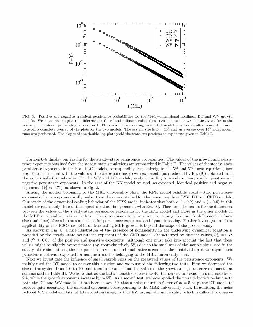
expect to find different positive and negative transient persistence exponents due to the fact that their morphologiesviolate the up–down interfacial symmetry with respect to the average level. No information about how differentthese two exponents should be is available in the literature. In most of these growth models, we observe that thetwo exponents are not very different from each other, especially during the transient regime. Fig. 3 shows thetransient regime results for DT and WV models, which are indeed very similar – their persistence probability curveshave almost identical behavior. We note here that the negative persistence probability has a faster decay than thepositive persistence probability. This indicates a negative sign of λ22, the coefficient that multiplies the nonlinearterm ∇2|∇h(r, t)|2 of the MBE equation. However, the relative order of the values of these exponents is reversedwhen λ22 > 0, which is the case in the CKD and KPK models, as shown in Fig. 4. To clarify this aspect, we show inFig. 5 the interfacial morphologies of DT and CKD models. We used a lattice of L = 104 sites (but only a portion of1000 sites is shown in each case) and the displayed configurations correspond to a time of 103 ML. The interface ofthe DT model is characterized by deep grooves, while the profile in the CKD model exhibits the distinct feature ofhigh pillars. Both morphologies display strong up–down interfacial asymmetry, but their representative features (i.e.deep grooves and high pillars) are opposite in “sign”, indicating a reversal of the sign of the coefficient λ22 (note thata reversal of the sign of λ22 in Eq. (5) is equivalent to changing the sign of the height variable h(r, t)).

As summarized in Table I, the DT, WV and CKD models show very similar values for the transient persistenceexponents when the above mentioned effect of the sign of λ22 is taken into account. However, some deviation fromthe exponent values for this group of models is observed in the RSOS KPK model which shows the smallest differencebetween the positive and negative persistence exponents. Finite size effects appear to be stronger in this case. Theseeffects also cause an increase in the measured values of the persistence exponents above the expected values. A similarbehavior is found in the steady–state results as well, as described below.

Our calculations of WV, DT, CKD and KPK persistence exponents illustrate the feasibility of studying this typeof nonequilibrium statistical probabilities for a large class of nonequilibrium applications described by nonlineardynamical equations. Until now, the only nonlinear equation for which persistence exponents have been calculated[24] is the KPZ equation which is arguably the simplest nonlinear Langevin equation. Further, the nonlinearity inthe KPZ equation becomes irrelevant in the steady–state regime in (1+1)–dimensions. So, the effects of nonlinearityare not reflected in the steady–state persistence behavior of (1+1)–dimensional KPZ systems. An immediate concernwould be that more complex nonlinear dynamic equations might be less approachable from the point of view ofpersistence probability calculation. Our results for four nonlinear models eliminate this possibility and illustrate theapplicability and usefulness of persistence probability calculations in the study of surface fluctuations.

12

100

101

102

103

t (ML)

10-3

10-2

10-1

100

P (

t)

DT: P+DT: P-WV: P+WV: P-

+_

FIG. 3: Positive and negative transient persistence probabilities for the (1+1)–dimensional nonlinear DT and WV growthmodels. We note that despite the difference in their local diffusion rules, these two models behave identically as far as thetransient persistence probability is concerned. The curves corresponding to the DT model have been shifted upward in orderto avoid a complete overlap of the plots for the two models. The system size is L = 104 and an average over 103 independentruns was performed. The slopes of the double–log plots yield the transient persistence exponents given in Table I.

Figures 6–8 display our results for the steady–state persistence probabilities. The values of the growth and persis-tence exponents obtained from the steady–state simulations are summarized in Table II. The values of the steady–statepersistence exponents in the F and LC models, corresponding, respectively, to the ∇2 and ∇4 linear equations, (seeFig. 6) are consistent with the values of the corresponding growth exponents (as predicted by Eq. (9)) obtained fromthe same small–L simulations. For the WV and DT models, as shown in Fig. 7, we obtain very similar positive andnegative persistence exponents. In the case of the KK model we find, as expected, identical positive and negativeexponents (θS

± ≈ 0.71), as shown in Fig. 2.Among the models belonging to the MBE universality class, the KPK model exhibits steady–state persistence

exponents that are systematically higher than the ones obtained for the remaining three (WV, DT and CKD) models.Our study of the dynamical scaling behavior of the KPK model indicates that both α (∼ 0.9) and z (∼ 2.9) in thismodel are reasonably close to the expected values, in agreement with Ref. [8]. Therefore, the reason for the differencesbetween the values of the steady–state persistence exponents for the KPK model and those in the other models inthe MBE universality class is unclear. This discrepancy may very well be arising from subtle differences in finitesize (and time) effects in the simulations for persistence exponents and dynamic scaling. Further investigation of theapplicability of this RSOS model in understanding MBE growth is beyond the scope of the present study.

As shown in Fig. 8, a nice illustration of the presence of nonlinearity in the underlying dynamical equation isprovided by the steady–state persistence exponents of the CKD model, characterized by distinct values, θS

+ ≈ 0.78

and θS− ≈ 0.66, of the positive and negative exponents. Although one must take into account the fact that these

values might be slightly overestimated (by approximatively 5%) due to the smallness of the sample sizes used in thesteady–state simulations, these exponents provide a good qualitative account of the nontrivial up–down asymmetricpersistence behavior expected for nonlinear models belonging to the MBE universality class.

Next we investigate the influence of small sample sizes on the measured values of the persistence exponents. Wemainly used the DT model to answer this question and we pursued the following two tests. First we decreased thesize of the system from 104 to 100 and then to 40 and found the values of the growth and persistence exponents, assummarized in Table III. We note that as the lattice length decreases to 40, the persistence exponents increase by ∼2%, while the growth exponents increase by ∼ 5%. As a second test, we have applied the noise reduction technique toboth the DT and WV models. It has been shown [39] that a noise reduction factor of m = 5 helps the DT model torecover quite accurately the universal exponents corresponding to the MBE universality class. In addition, the noisereduced WV model exhibits, at late evolution times, its true EW asymptotic universality, which is difficult to observe

13

100

101

102

103

t (ML)

10-4

10-3

10-2

10-1

P (

t)

CKD: P+CKD: P-KPK: P+KPK: P-

+_

FIG. 4: Positive and negative transient persistence probabilities for the (1+1)–dimensional CKD (the upper two curves) andRSOS (the lower two, almost overlapped curves) models that belong to MBE universality class. In both cases the system sizewas L = 104 and an average over 103 independent runs was performed. The slopes of the double–log plots yield the transientpersistence exponents given in Table I.

L θT+ θT

− β

104 0.95 ± 0.02 0.98 ± 0.02 0.38 ± 0.01

102 0.96 ± 0.02 0.99 ± 0.02 0.37 ± 0.01

40 0.98 ± 0.02 1.01 ± 0.02 0.36 ± 0.01

TABLE III: Transient positive and negative persistence exponents, θT±, obtained for the DT model with different system sizes

(L). The effect of the system size on the measured growth exponent, β, is displayed in the last column. No result for steady–state persistence exponents is available for system sizes larger than ∼ 100, due to the impossibility of reaching saturation ofthe interface width for such values of L in time scales accessible in simulations. The results shown here were averaged over 500(for L = 104), 5 × 104 (for L = 100) and 105 (for L = 40) independent runs.

without applying noise reduction. Therefore, the DT model with the appropriate noise reduction factor is expectedto provide the correct persistence exponents associated with the fourth–order nonlinear dynamical equation for MBEgrowth. The results obtained from the simulations with noise reduction are summarized in Table IV. We notice thatthe noise reduction scheme produces only a minor change in the persistence exponents and in addition, the resultsobtained for m = 5 agree within the error bars with those for the CKD model. We, therefore, conclude that thenoise reduced DT model and the discrete CKD model provide a good representation of the MBE universality class,characterized by two different steady–state persistence exponents: θS

+ ∼ 0.66 (positive persistence) and θS− ∼ 0.78

(negative persistence). These nontrivial persistence exponents for this class have not been reported earlier, and itwould be useful to check these results from further theoretical or experimental studies. Regarding the noise reducedWV model we mention that the convergence of θS towards the expected value of 3/4 is rather slow in the case of thepositive exponent and probably a higher value of the noise reduction factor would be necessary to reveal the true EWuniversality. We did not explore this technical issue any further.

We note that among the positive and negative steady–state persistence exponents for these nonlinear growth models,the smaller one (for example, the positive exponent in the DT model or the negative exponent of the CKD model),turns out to be close to (1 − β). In the next subsection, we show analytically that this relation between the smallersteady-state persistence exponent and the dynamic growth exponent is, in fact, exact. Our numerical studies suggesta connection of this result with the morphology that develops in the steady–state regime. As shown in Fig. 5, thecharacteristic feature of the DT morphology is the presence of deep grooves, while the CKD model exhibits highpillars. Loosely speaking, in the case of the DT model, we expect the relation of Eq. (9) to be more likely to besatisfied by the positive persistence exponent than the negative one because the preponderant grooves, responsible forthe negative persistence exponent, represent the effects of the nonlinearity of the underlying MBE dynamics. More

14

0 200 400 600 800 1000Lattice position

-40

-20

0

20

40

Inte

rfac

ial h

eigh

t

DT: t=1000 ML

0 200 400 600 800 1000Lattice position

-40

-20

0

20

40

Inte

rfac

ial h

eigh

t

CKD: t=1000 ML

FIG. 5: Morphologies of the (1+1)–dimensional DT (top) and CKD (bottom) stochastic models for L = 104 (only a portionof 1000 sites is shown) and t = 103 ML. In the DT model, we notice a breaking of up–down symmetry due to the formation ofdeep grooves, while in the CKD model, the representative asymmetric feature corresponds to high pillars.

work is clearly needed for a better understanding of the possible relationship between such “nonlinear” features ofthe interface morphology and the value of the persistence exponent.

B. An exact relation between steady-state persistence exponents and the growth exponent

As mentioned earlier, for interface heights h(r, t) evolving via a Langevin equation that preserves (h → −h)symmetry (for example, any linear Langevin equation), the steady state persistence exponents satisfy the scalingrelation θS

+ = θS− = 1 − β, where β is the growth exponent [23]. In this subsection, we derive a generalized scaling

relation,

β = max[

1 − θS+, 1 − θS

−

]

, (14)

which is valid even in the absence of (h → −h) symmetry. When this symmetry is restored, Eq. (14) reduces to theknown result [23], θS

+ = θS− = 1 − β.

15

100

101

102

103

t (ML)

10-3

10-2

10-1

P (

t)

F: P+F: P-LC: P+LC: P-

+_

FIG. 6: Positive and negative steady–state persistence probabilities for the (1+1)–dimensional F and LC models which aregoverned by linear continuum dynamical equation. The temporal decay of the persistence probability is slower in the LC modelwhich has a larger growth exponent (βLC = 3/8, βF = 1/4). We used L = 1000 and t0 = 4 × 106 ML for the F model, andL = 40, t0 = 106 ML for the LC model. The displayed results were averaged over 5000 independent runs. The measured slopesof the double–log plots yield the steady–state persistence exponents shown in Table II.

100

101

102

103

t (ML)

10-2

10-1

100

P (

t)

DT: P+DT: P-WV: P+WV: P-

+_

FIG. 7: Steady–state persistence probabilities for two (1+1)–dimensional models in the MBE universality class – the DT andWV models. As in the transient case, these two models exhibit almost identical persistence behavior in the steady state. Theeffects of the nonlinearity in their continuum dynamical description are not very prominent for the small lattice sizes consideredhere. For the data shown, systems of size L = 40 were equilibrated for t0 = 105 ML, and the results were averaged over 5000independent runs. The persistence plots for the DT model have been shifted up in order to make them distinguishable fromthe WV plots. The measured slopes of the double–log plots yield the steady–state persistence exponents shown in Table II.

16

100

101

102

103

t (ML)

10-3

10-2

10-1

100

P (

t)

CKD: P+CKD: P-KPK: P+KPK: P-

+_

FIG. 8: Double–log plots of the steady–state persistence probabilities of (1+1)–dimensional MBE class CKD and KPK (shiftedup by a constant amount) models. While the KPK model does not show a clear effect of nonlinearity in the values of thepersistence exponents, the CKD model shows positive and negative persistence exponents that are clearly different from eachother. Systems of size L = 40 (CKD) and L = 200 (KPK) were equilibrated for t0 ∼ 105 ML. The results were averagedover 104 independent runs. The measured slopes of the double–log plots yield the steady–state persistence exponents shown inTable II.

Growth model m θS+ θS

−

DT 1 0.64 ± 0.02 0.72 ± 0.01

DT 5 0.65 ± 0.02 0.77 ± 0.01

WV 1 0.65 ± 0.02 0.70 ± 0.01

WV 5 0.68 ± 0.02 0.75 ± 0.01

TABLE IV: Positive and negative persistence exponents, θS±, for the steady state of the DT and WV models for two different

values of the noise reduction factor, m. Systems of size L = 40 were equilibrated for 105 ML and the results were averagedover 5000 independent runs.

To derive the relation in Eq. (14), we start with a generic interface described by a height field h(r, t) and define therelative height, u(r, t) = h(r, t) − h(r, t) where h(r, t) =

∫

h(r, t)dr/V is the spatially averaged height and V is thevolume of the sample. Let us also define the incremental auto-correlation function in the stationary state,

C(t, t′) = limt0→∞

〈[u(r, t + t0) − u(r, t′ + t0)]2〉. (15)

It turns out that for generic self-affine interfaces (which do not have to be Gaussian), this function C(t, t′) depends onlyon the time difference |t− t′| (and not on the individual times t and t′) in a power-law fashion for large |t− t′| [24, 49],

C(t, t′) ∼ |t − t′|2β , (16)

where β is the growth exponent.This particular behavior of the auto-correlation function in Eq. (16) is typical of a fractional Brownian motion

(fBm). A stochastic process x(t) with zero mean is called an fBm if its incremental correlation function C(t1, t2) =〈[x(t1) − x(t2)]

2〉 depends only on the time difference |t1 − t2| in a power-law fashion for large arguments [50],

C(t1, t2) = 〈[x(t1) − x(t2)]2〉 ∼ |t1 − t2|

2H , (17)

where 0 < H < 1 is called the Hurst exponent of the fBm. For example, an ordinary Brownian motion which evolvesas dx/dt = η(t) where η(t) is a Gaussian white noise with zero mean and a delta function correlator, satisfies Eq. (17)

17

with H = 1/2. Thus an ordinary Brownian motion is a fBm with H = 1/2. It follows clearly by comparing Eqs. (16)and (17) that the relative height u(r, t) of a generic interface at a fixed point r in space, in its stationary state, is alsoa fBm with Hurst exponent, H = β. Note that an fBm is not necessarily Gaussian.

We are then interested in the ‘no return probability’ to the initial value of the fBm process u(r, t). So, the relevantrandom process is Y (r, t) = u(r, t + t0)− u(r, t0). Clearly, Y (r, t) is also a fBm with the same Hurst exponent β sincethe incremental correlation function of Y is the same as that of u(r, t). We are then interested in the zero crossingproperties of the fBm Y (r, t). Now, consider the process Y (r, t) as a function of time, at a fixed point r in space,from time t0 to time t0 + t where t0 → ∞. There are two types of intervals between successive zero crossings in time,the ‘+’ type (where the process lies above 0) and the ‘−’ type (where the process lies below 0).

In general, the statistics of the two types of intervals are different. Only, in special cases, where one has theadditional knowledge that the process Y (r, t) is symmetric around 0 (i.e., processes which preserve the (h → −h)symmetry), the + and − intervals will have the same statistics. For such cases, a simple scaling argument was given

in Ref. [23] to show that the length of an interval of either type has a power-law distribution, Q(τ) ∼ τ−1−θS

(forlarge τ) with θS = 1−H = 1−β. Note that this relation between the persistence exponent and the Hurst exponent isvery general and holds for any symmetric fBm, i.e., any stochastic process with zero mean (not necessarily Gaussian)satisfying Eq. (17). Recently, other applications of this result have been found [51, 52]. For general nonsymmetric

processes, however, one would expect that Q±(τ) ∼ τ−1−θS

± for large τ , where θS+ and θS

− are, in general, different.Here we generalize this scaling argument of Ref. [23] (derived for a symmetric process) to include the nonsymmetriccases and derive the result in Eq. (14).

The derivation of Eq. (14) follows more or less the same line of arguments as that used in Ref. [23] for the symmetriccase. Let P (Y, τ) denote the probability that the process has value Y at time τ , given that it starts from its initialvalue 0 at τ = 0. Then, it is natural to assume that the normalized probability distribution P (Y, τ) has a scalingform,

P (Y, τ) =1

σ(τ)f

(

Y

σ(τ)

)

, (18)

where σ(τ) is the typical width of the process, σ2(τ) = 〈Y 2(τ)〉. It follows from Eq. (16) that σ(τ) ∼ τβ for large τ .The scaling function f(z) is a constant at z = 0, f(0) ∼ O(1) (note that, in general, f(z) is not a symmetric functionof z) and should decrease to 0 as z → ±∞. So, given that a zero occurs initially, the probability ρ(τ) = P (0, τ) thatthe process will return to 0 after time τ (not necessarily for the first time) scales as

ρ(τ) ∼1

σ(τ)∼ τ−β , (19)

as τ → ∞. This function ρ(τ) indeed is the density of zero crossings between τ and τ + dτ . Thus, the total numberof zeros upto a time T is simply the integral,

N(T ) =

∫ T

0

ρ(τ)dτ ∼ T 1−β, (20)

for large T .Next, we relate the persistence probabilities to the number of zeros. Let P±(τ) denote the probabilities that the

process stays positive (or negative) over the interval [0, τ ], given that it started from a zero. By definition, we have

P±(τ) ∼ τ−θS

± for large τ . Then, Q±(τ) = −dP±(τ)/dτ ∼ τ−1−θS

± (as τ → ∞) denote the probabilities that theprocess will cross zero next time (from the positive or the negative side respectively) between time τ and τ + dτ .Thus, Q±(τ) are also the distribution of intervals of the two types of length τ .

Now, consider a total length of time T . Let N(T ) denote the total number of intervals in this period, half of themare + types and the other half − types, N±(T ) = N(T )/2. Let, n±(τ) denote the number of ± intervals of lengthτ within the period T . Thus, the fraction of + (or −) intervals of length τ , n±(τ)/N±(τ), by definition, are the twodistributions Q±(τ) provided T is large. Thus, for large T , we have

n±(τ, T ) =N(T )

2Q±(τ) ∼ N(T )τ−1−θS

± , (21)

for 1 << τ ≤ T . On the other hand, we have the length conservation condition (the total length covered by theintervals must be T ),

∫ T

0

dτ τ [n+(τ) + n−(τ)] = T. (22)

18

Substituting the asymptotic behavior of n±(τ) in Eq.(21) into the left-hand side of Eq.(22), we get

N(T )

[

T 1−θS

+

1 − θS+

+T 1−θS

−

1 − θS−

]

∝ T. (23)

We next use N(T ) ∼ T 1−β for large T from Eq.(20). This gives, for large T ,

[

T 1−θS

+

1 − θS+

+T 1−θS

−

1 − θS−

]

∼ T β. (24)

Taking T → ∞ limit and matching the leading power of T in Eq. (24), we arrive at our main result in Eq. (14). Notethat in the above derivation we have implicitly assumed a small-t cut-off and focused only on the distribution of largeintervals. Our numerical results obtained for a class of nonlinear interfaces in both (1 + 1) and (2 + 1) dimensions(see Sec. IVD below) are consistent with the analytical result in Eq. (14).

C. Dependence of persistence probabilities on the initial configuration

We present in this section some surprising simulation results about the dependence of the persistence behavior(specifically, the values of the persistence exponents) on the choice of the initial configuration. In particular, weshow that the steady–state exponents may be obtained with a fair degree of accuracy from simulations in which theinterface has not yet reached the steady state. We also present some results that have bearing on the measurabilityof the transient persistence exponents from experimental data.

We recall that in Section IVA the transient persistence exponents were measured from simulations in which theinitial configuration was completely flat, corresponding to t0 = 0. To examine the dependence of the persistenceprobabilities on the choice of t0, we evolved samples governed by F and DT atomistic diffusion rules for t0 = 10, 100and 1000 ML, starting from perfectly flat initial states and used the resulting configurations as starting points formeasuring the persistence probability (the probability of the height at a given site not returning to its initial valueat time t0) as a function of t. We show the results of these simulations in Figs. 9 and 10 for the F and DT models,respectively. We find that even for the small value of t0 = 10 ML [see panel a)], the observed persistence probabilitiesdo not exhibit power law decay in time with the transient persistence exponents, despite the fact that the expectedcondition [23] for transient behavior, t ≫ t0, is well satisfied in a large part of the range of t used in these simulations.These results point out a practical difficulty in obtaining experimental evidence for transient persistence behavior.Since perfectly flat initial configurations can hardly be achieved experimentally and experimental measurements arealways started from a relatively rough substrate, the transient persistence exponents may very well not be measurablefrom experiments if the only way of measuring these exponents is to start from a perfectly flat morphology.

As the value of t0 is increased to 100 ML, the persistence probabilities tend to show the expected power law behavior,as shown in Fig. 9(b) for the F model and in Fig. 10(b) for the DT model. Most surprisingly, as shown in Figs. 9(c)

and 10(c), we find that for t0 = 1000 ML, one recovers precisely the power law behavior, P (t0, t0 + t) ∝ t−θS

, and theexponents are essentially the same as the previously obtained steady–state ones shown in Table II. This investigation,thus, reveals the fact that a measurement of the steady–state persistence exponents does not require the preparationof an initial state in the long–time steady–state regime where the interface width has reached saturation: an initialstate in the pre–asymptotic growth regime where the interface width is still increasing as a power law in time [asillustrated in Figs. 9(d) and 10(d)] is sufficient for measurements of the steady–state persistence exponents. A similarresult was reported in Ref. [23], but it was argued there that the measurement time t must be much smaller than t0 forsteady–state persistence behavior to be observed. Our results show that the steady–state persistence exponents arefound even if t is of the order of (or even slightly larger than) the initial time t0. This observation has an importantpractical benefit: it implies that one can easily obtain accurate estimates of the steady–state persistence exponentsusing rather large systems (L ∼ 104), and growing approximately up to t0 ∼ 103 ML, instead of having to use thevery large values (of the order of Lz) of t0 necessary for obtaining saturation of the interface width. At the same time,this observation also illustrates the above mentioned difficulty in obtaining the transient exponents from experimentalmeasurements.

To investigate the effects of random imperfections in the initial substrate (which are always present in experimentalstudies) on the persistence behavior, we carried out simulations in which particles were deposited randomly on aperfectly flat substrate for 10 ML and the resulting configuration was used for further depositions using the diffusionrules of the F and DT models. Persistence probabilities were calculated starting from the configurations obtainedafter the random deposition of 10 ML. Figures 11 and 12 show the results for the F and DT models, respectively. We

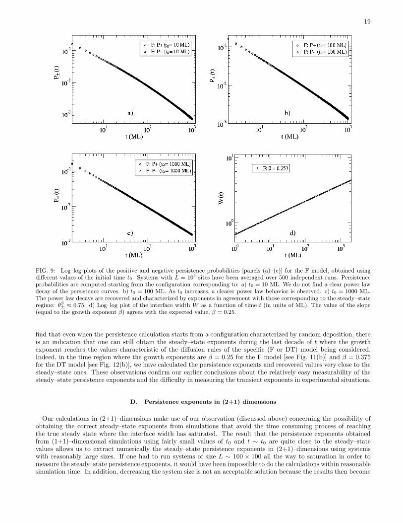
19

FIG. 9: Log–log plots of the positive and negative persistence probabilities [panels (a)–(c)] for the F model, obtained usingdifferent values of the initial time t0. Systems with L = 104 sites have been averaged over 500 independent runs. Persistenceprobabilities are computed starting from the configuration corresponding to: a) t0 = 10 ML. We do not find a clear power lawdecay of the persistence curves. b) t0 = 100 ML. As t0 increases, a clearer power law behavior is observed. c) t0 = 1000 ML.The power law decays are recovered and characterized by exponents in agreement with those corresponding to the steady–stateregime: θS

± ≈ 0.75. d) Log–log plot of the interface width W as a function of time t (in units of ML). The value of the slope(equal to the growth exponent β) agrees with the expected value, β = 0.25.

find that even when the persistence calculation starts from a configuration characterized by random deposition, thereis an indication that one can still obtain the steady–state exponents during the last decade of t where the growthexponent reaches the values characteristic of the diffusion rules of the specific (F or DT) model being considered.Indeed, in the time region where the growth exponents are β = 0.25 for the F model [see Fig. 11(b)] and β = 0.375for the DT model [see Fig. 12(b)], we have calculated the persistence exponents and recovered values very close to thesteady–state ones. These observations confirm our earlier conclusions about the relatively easy measurability of thesteady–state persistence exponents and the difficulty in measuring the transient exponents in experimental situations.

D. Persistence exponents in (2+1) dimensions

Our calculations in (2+1)–dimensions make use of our observation (discussed above) concerning the possibility ofobtaining the correct steady–state exponents from simulations that avoid the time consuming process of reachingthe true steady state where the interface width has saturated. The result that the persistence exponents obtainedfrom (1+1)–dimensional simulations using fairly small values of t0 and t ∼ t0 are quite close to the steady–statevalues allows us to extract numerically the steady–state persistence exponents in (2+1)–dimensions using systemswith reasonably large sizes. If one had to run systems of size L ∼ 100 × 100 all the way to saturation in order tomeasure the steady–state persistence exponents, it would have been impossible to do the calculations within reasonablesimulation time. In addition, decreasing the system size is not an acceptable solution because the results then become

20

FIG. 10: Positive and negative persistence probabilities [panels (a)–(c)] for the DT model, obtained using different values ofthe initial time t0. Persistence probabilities are computed starting from the configuration corresponding to: a) t0 = 10 ML.As in the case of the F model, we do not find a clear power law for the persistence curves. b) t0 = 100 ML; c) t0 = 1000 ML:Power law decays are recovered and characterized by exponents that are approximately equal to those corresponding to thesteady–state regime, θS

+ ≈ 0.64 and θS− ≈ 0.71. d) Log–log plot of the interface width W as a function of time t (in units of

ML). The slope gives a growth exponent of βDT ≃ 0.375.

dominated by finite size effects.Simulations for (2+1)–dimensional discrete growth models were carried out for the F model (β = 0) and the DT

model (β ≃ 1/5). Simulations using systems of size L = 200× 200 revealed that the growth exponents, obtained fromaverages over 200 independent runs, are β = 0.04 ± 0.01 and 0.20 ± 0.01 for the F and DT models, respectively, inagreement with Ref. [42]. In the DT model, we noticed a crossover from the initial value of 0.26 to the asymptoticexpected value of 0.20, indicating that no additional noise reduction technique is necessary for obtaining results thatreflect the correct universality class of this model. For both F and DT models we calculate the transient and steady–state persistence probabilities by recording the fraction of sites which do not return to their initial height up to timet, as in the (1+1)–dimensional case. We used t0 = 0 (perfectly flat initial state) in the calculation of the transientpersistence probabilities, and three different values, such as t0 = 20 ML, 200 ML and 2000 ML for the F model, inthe calculation of the steady–state exponents.

We report the results for the transient probabilities just for the sake of completeness: the rapid decay of thepersistence probabilities prevents us from obtaining accurate values of the associated persistence exponents. This fastdecay of the transient persistence probability is a consequence of the reduced roughness of these higher dimensionalmodels. This effect is particularly pronounced for the F model for which the persistence exponent is found to belarger than 6 and the persistence probability decreases rapidly to zero for any deposition time larger than ∼ 60 ML,as shown in Fig. 13. We also observe that the transient values of the positive and negative persistence exponentsin the DT model are roughly 3 times larger than the values obtained in the (1 + 1)–dimensional case. The relativedifference between the positive and negative persistence exponents remains approximately the same as that in the(1+1)–dimensional model. Our results for these (2+1)–dimensional persistence exponents are summarized in Table

21

101

102

103

t (ML)

10-2

10-1

100

P

(t)

F (RD substrate): P+F (RD substrate): P-

+_

101

102

103

t (ML)

100

101

W(t

)

F (t = 10 RD ML): = 0.250 β

a) b)

FIG. 11: a) Positive and negative persistence probabilities for the F model. During the deposition of the first 10 ML, thegrowth process is random deposition. The diffusion rules of the F model are then used to evolve the interface. Persistenceprobabilities are computed starting from the configuration obtained after the random deposition of 10 ML. The positive andnegative persistence exponents in the last growth decade are in the range 0.6 to 0.7, depending on the fitting region. b)Log–log plot of the interface width W as a function of t (in ML). The slope in the first decade of t is precisely the random–deposition value, β = 0.5. The second decade shows a crossover region where the systems undergoes a transformation towardsa morphology governed by the F model diffusion rules, and the last decade is characterized by the expected growth exponentof the F model, β = 0.25.

101

102

103

t (ML)

10-2

10-1

P (

t)

DT (RD substrate): P+DT (RD substrate): P-

+_

101

102

103

t (ML)

100

101

W(t

)DT (t = 10 RD ML): = 0.3750 β

a) b)

FIG. 12: Positive and negative persistence probability curves for the DT model. During the deposition of the first 10 ML,the growth process is random deposition. The diffusion rules of the DT model are used to evolve the interface subsequently.Persistence probabilities are computed starting from the configuration obtained after the deposition of the first 10 ML. Thepositive and negative persistence exponents in the last growth decade are approximatively equal to 0.66 and 0.79 respectively.b) Log–log plot of the interface width W as a function of time t (in ML). Beyond the crossover regime, the last decade in t ischaracterized by the expected growth exponent of the DT model, β ≃ 0.375.

V.We now focus on the steady–state persistence exponents which, as discussed above, are found using relatively small

values of t0 and t ≈ t0. In Fig. 14(a), we show that for t0 ≪ t (e.g. for t0 = 20 ML), the persistence probability of theF model does not exhibit a clear power law decay. However panels b) and c) of Fig. 14 reveal that once t0 becomes ofthe order of the measurement time t, the expected power law is recovered and in addition the steady–state exponentfor the linear F model, θS = 1.01 ± 0.02, which should be equal to (1 − β) with β = 0, is recovered. The results forthe DT model are presented in Fig. 15. The steady–state persistence exponents have been measured from the powerlaw decays shown in Fig. 15(b). In this temporal regime, as shown in panel d), the growth exponent is equal to theasymptotic value of 1/5. The persistence behavior of the DT model in this regime is characterized by θS

+ ≈ 0.76 and

θS− ≈ 0.85, indicating that the relation of Eq. (14) holds reasonably well for the (2+1)– dimensional nonlinear MBE

22

101

102

103

t (ML)

10-6

10-4

10-2

P

(t)

DT: P-DT: P+F: P+F: P-

+_

FIG. 13: Transient persistence probabilities for the (2+1)–dimensional F and DT growth models. In the case of the F model,systems of size L = 1000 × 1000 have been averaged over 200 independent runs, while for the DT model, systems of sizeL = 500 × 500 have been averaged over 800 independent runs. The transient persistence probability for the F model exhibitsa very fast decay, characterized by a persistence exponent θT

≈ 6.9 for the last decade of t. More accurate results (see TableV) are obtained for the exponents in the DT model, although the statistics is not excellent.

Growth model L θT+ θT

− θS+ θS

− β

FM 200 × 200 > 6 > 6 1.02 ± 0.02 1.00 ± 0.02 0.04 ± 0.01

DT 200 × 200 2.84 2.44 0.76 ± 0.02 0.85 ± 0.02 0.20 ± 0.01

TABLE V: Transient and steady–state persistence exponents, θ±, for two (2+1)–dimensional discrete growth models. Themeasured value of the growth exponent β is shown in the last column. The transient persistence exponents are measured withrelatively low accuracy due to the rapid temporal decay of the persistence probabilities.

dynamics, as in the (1 + 1)–dimensional case. It is important to mention that the same values of the persistenceexponents have been obtained using a DT system with L = 40 × 40, equilibrated for t0 = 105 ML, as required in thetraditional method (used in most of the (1+1)–dimensional simulations) of measuring the steady–state persistenceprobabilities. Thus the “quick and easy” method of obtaining the steady–state persistence exponent again agrees wellwith the exponent extracted from the actually saturated interface, as discussed above.

We have also performed some preliminary persistence calculations for the (2+1)–dimensional CKD model in order tocheck the validity of our reported (2+1)–dimensional MBE persistence exponents. Using L = 100×100 and t0 = 1000ML, we find that the values of the positive and negative persistence exponents depend to some extent on the chosenvalues for the coefficient λ22 of the nonlinear term and the control parameter c. For example, we obtain θS

+ ≈ 0.82 and

θS− ≈ 0.77 using λ22 = 5.0 and c = 0.085, and θS

+ ≈ 0.88 and θS− ≈ 0.83 using λ22 = 5.0 and c = 0.13. Both cases are

characterized by a growth exponent of 0.18± 0.01, in agreement with Ref. [53], which is consistent with the expectedvalue of 1/5. The results obtained in the latter case are displayed in panel c) of Fig. 15 for the purpose of illustratingthe similarity between the DT and CKD models. From these observations, we conclude that the (2+1)–dimensionalDT and CKD persistence results are consistent with each other and they clearly reflect the nonlinearity of the MBEdynamical equation in the difference between the values of the positive and negative persistence exponents as expectedfor the up–down asymmetric generic nonlinear situation.

E. Scaling behavior of the persistence probability

Since all the results described above have been obtained from simulations of finite systems, it is important to addressthe question of how the persistence probabilities are affected by the finite system size. We have already encounteredsuch effects in our study of persistence probabilities for (1+1)–dimensional models (see Table III), where it was foundthat the measured values of the persistence exponents in the steady state increase slightly as the system size L is

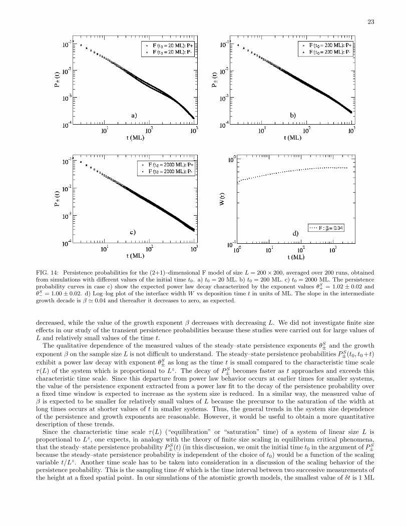
23

FIG. 14: Persistence probabilities for the (2+1)–dimensional F model of size L = 200× 200, averaged over 200 runs, obtainedfrom simulations with different values of the initial time t0. a) t0 = 20 ML. b) t0 = 200 ML. c) t0 = 2000 ML. The persistenceprobability curves in case c) show the expected power law decay characterized by the exponent values θS

+ = 1.02 ± 0.02 andθS− = 1.00 ± 0.02. d) Log–log plot of the interface width W vs deposition time t in units of ML. The slope in the intermediate

growth decade is β ≃ 0.04 and thereafter it decreases to zero, as expected.

decreased, while the value of the growth exponent β decreases with decreasing L. We did not investigate finite sizeeffects in our study of the transient persistence probabilities because these studies were carried out for large values ofL and relatively small values of the time t.

The qualitative dependence of the measured values of the steady–state persistence exponents θS± and the growth

exponent β on the sample size L is not difficult to understand. The steady–state persistence probabilities PS±(t0, t0+t)

exhibit a power law decay with exponent θS± as long as the time t is small compared to the characteristic time scale

τ(L) of the system which is proportional to Lz. The decay of PS± becomes faster as t approaches and exceeds this

characteristic time scale. Since this departure from power law behavior occurs at earlier times for smaller systems,the value of the persistence exponent extracted from a power law fit to the decay of the persistence probability overa fixed time window is expected to increase as the system size is reduced. In a similar way, the measured value ofβ is expected to be smaller for relatively small values of L because the precursor to the saturation of the width atlong times occurs at shorter values of t in smaller systems. Thus, the general trends in the system size dependenceof the persistence and growth exponents are reasonable. However, it would be useful to obtain a more quantitativedescription of these trends.

Since the characteristic time scale τ(L) (“equilibration” or “saturation” time) of a system of linear size L isproportional to Lz, one expects, in analogy with the theory of finite size scaling in equilibrium critical phenomena,that the steady–state persistence probability PS

±(t) (in this discussion, we omit the initial time t0 in the argument of PS±

because the steady–state persistence probability is independent of the choice of t0) would be a function of the scalingvariable t/Lz. Another time scale has to be taken into consideration in a discussion of the scaling behavior of thepersistence probability. This is the sampling time δt which is the time interval between two successive measurements ofthe height at a fixed spatial point. In our simulations of the atomistic growth models, the smallest value of δt is 1 ML

24

FIG. 15: Persistence probabilities for the (2+1)–dimensional DT model of size L = 200×200, averaged over 200 runs, obtainedfrom simulations with different values of the initial time t0. a) t0 = 200 ML: The persistence probabilities do no exhibit clearpower law decay. b) t0 = 4000 ML: The persistence probability curves show the expected power law decay characterized bythe exponent values θS

+ = 0.77 ± 0.02 and θS− = 0.85 ± 0.02. c) Results for the (2+1)–dimensional CKD model, obtained using

L = 100× 100, t0 = 1000 ML, λ = 5 and c = 0.13. d) Log–log plot of the interface width W vs deposition time t in ML for theDT model. The slope manifests a crossover from an initial value of ∼ 0.26 to the asymptotic value of 0.20.

because the heights are measured after each deposition of one complete (ideal) monolayer. However, larger integralvalues of δt can also be used in the calculation of the persistence probabilities. Since experimental measurements arealso carried out at discrete time intervals, the presence of a finite value of δt has to be accounted for in the analysisof experimental data also. Note that the persistence probability itself is mathematically defined, P (t0, t0 + t), forcontinuous values of time t whereas measurements and simulations are necessarily done on discrete time.

It has been pointed out in Ref. [54] that discrete–time sampling of a continuous–time stochastic process does affectthe measured persistence probability. Such effects have been investigated in detail [40] in the context of a differentstochastic probability (called the survival probability in Ref. [40]) that measures the probability of the interface heightat a fixed position not returning to its time–averaged value within time t. In that work, it was found that the survivalprobability measured for a system of size L with sampling interval δt is a function of the scaling variables t/Lz andδt/Lz. We expect a similar behavior for the steady–state persistence probabilities measured in our simulations. Thus,the expected scaling behavior of PS

±(t, L, δt) is

PS±(t, L, δt) = f±(t/Lz, δt/Lz), (25)

where the function f±(x1, x2) should decay as x−θS

±

1 for small x1 and x2 ≪ 1.To test the validity of this scaling ansatz, we have carried out calculations of the steady–state persistence probability

in the linear F model (the positive and negative persistence probabilities are the same in this model) using differentvalues of L and δt. Due to the linearity of the F model, we have computed a persistence probability PS(t) given bythe average value of the positive and negative persistence probabilities. If the scaling description of Eq. (25) is valid,

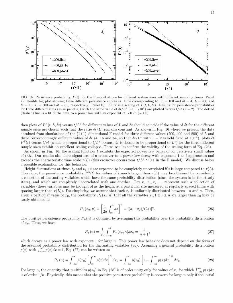
25

FIG. 16: Persistence probability, P (t), for the F model shown for different system sizes with different sampling times. Panela): Double–log plot showing three different persistence curves vs. time corresponding to: L = 100 and δt = 4, L = 400 andδt = 16, L = 800 and δt = 81, respectively. Panel b): Finite size scaling of P (t, L, δt). Results for persistence probabilitiesfor three different sizes (as in panel a)) with the same value of δt/Lz (i.e. 1/104) are plotted versus t/δt (z = 2). The dotted(dashed) line is a fit of the data to a power law with an exponent of ∼ 0.75 (∼ 1.0).

then plots of PS(t, L, δt) versus t/Lz for different values of L and δt should coincide if the value of δt for the differentsample sizes are chosen such that the ratio δt/Lz remains constant. As shown in Fig. 16 where we present the dataobtained from simulations of the (1+1)–dimensional F model for three different values (200, 400 and 800) of L andthree correspondingly different values of δt (4, 16 and 64, so that δt/Lz with z = 2 is held fixed at 10−4), plots ofPS(t) versus t/δt (which is proportional to t/Lz because δt is chosen to be proportional to Lz) for the three differentsample sizes exhibit an excellent scaling collapse. These results confirm the validity of the scaling form of Eq. (25).

As shown in Fig. 16, the scaling function f exhibits the expected power law behavior for relatively small valuesof t/δt. Our results also show signatures of a crossover to a power law decay with exponent 1 as t approaches andexceeds the characteristic time scale τ(L) (this crossover occurs near t/Lz ≃ 0.1 in the F model). We discuss belowa possible explanation for this behavior.

Height fluctuations at times t0 and t0 + t are expected to be completely uncorrelated if t is large compared to τ(L).Therefore, the persistence probability PS(t) for values of t much larger than τ(L) may be obtained by consideringa collection of fluctuating variables which have the same probability distribution (since the system is in the steadystate), and which are completely uncorrelated with one another. Let x0, x1, x2, . . . represent such a collection ofvariables (these variables may be thought of as the height at a particular site measured at regularly spaced times withspacing larger than τ(L)). For simplicity, we assume that each xi is uniformly distributed between −a and a. Then,given a particular value of x0, the probability P+(x0, n) that all the variables xi, 1 ≤ i ≤ n are larger than x0 may beeasily obtained as

P+(x0, n) =

[

1

2a

∫ a

x0

dx

]n

= [(a − x0)/(2a)]n. (26)

The positive persistence probability P+(n) is obtained by averaging this probability over the probability distributionof x0. Thus, we have

P+(n) =1

2a

∫ a

−a

P+(x0, n)dx0 =1

n + 1, (27)

which decays as a power law with exponent 1 for large n. This power law behavior does not depend on the form ofthe assumed probability distribution for the fluctuating variables {xi}. Assuming a general probability distributionp(x) with

∫ ∞

−∞p(x)dx = 1, Eq. (27) can be written as

P+(n) =

∫ ∞

−∞

p(x0)

[∫ ∞

x0

p(x)dx

]n

dx0 =

∫ ∞

−∞

p(x0)

[

1 −

∫ x0

−∞

p(x)dx

]n

dx0. (28)

For large n, the quantity that multiplies p(x0) in Eq. (28) is of order unity only for values of x0 for which∫ x0

−∞p(x)dx

is of order 1/n. Physically, this means that the positive persistence probability is nonzero for large n only if the initial

26

value x0 is very close to the lower limit of the allowed range of values. This effectively restricts the upper limit of theintegral over x0 to y0 where y0 satisfies the requirement that

∫ y0

−∞

p(x)dx = C/n, (29)

where C is a constant of order unity. Since the quantity that multiplies p(x0) in Eq. (28) is of order unity for suchvalues of x0, it follows that

P+(n) ≈

∫ y0

−∞

p(x0)dx0 ∝1

n. (30)

This simple analysis shows that the simulation results for the behavior of the scaling function of Fig. 16 for largevalues of t/δt are quite reasonable.

While we have not carried out similar scaling analyses [Eq. (25)] for other models, we expect the scaling form ofEq. (25) to be valid in general. We expect that such scaling analysis of the persistence probability as a function ofthe system size L and the sampling time δt would be useful in the analysis of numerical and experimental data inthe future. In fact, we believe that a direct experimental verification of the scaling ansatz defined by Eq. (25) will bevaluable.

V. CONCLUDING REMARKS

In this paper we have investigated the temporal first passage statistics, expressed in terms of temporal persistenceprobabilities, for a variety of atomistic models that provide discrete realizations of several linear and nonlinear Langevinequations for the stochastic dynamics of growing and fluctuating interfaces. Using extensive kinetic Monte Carlosimulations, we have obtained transient and steady–state persistence exponents for these (1+1) and (2+1)–dimensionalSOS and RSOS growth models. We have followed the methodology of Krug et al. [23, 24] and extended their numericalwork to the nonlinear MBE dynamical equation by studying the persistence behavior of the atomistic DT, WV, CKDand KPK models. From these studies, we have identified two persistence exponents for each of the two temporalregimes (transient and steady–state) of the persistence probability. The difference between the values of the twoexponents reflects the nonlinearity (and the resulting lack of up–down symmetry) of the MBE dynamical equation.

Among the models studied here, we find that in (1+1) dimensions and in the range of system sizes used in oursimulations, WV and DT models are hardly distinguishable from the point of view of transient and steady–statepersistence behavior: the persistence exponents obtained for these two models are very close to each other. We,therefore, conclude that in the range of simulation parameters used in this study, the (1+1)–dimensional DT and WVmodels belong to the same universality class (namely the MBE universality class) as far as their persistence behavior isconcerned. A separate investigation is required in order to understand the universality class of the WV model in (2+1)dimensions. The KPK model appears not to reflect well the nonlinear feature of the underlying dynamical equationin the values of the positive and negative persistence exponents. This is probably due to strong finite size effectsarising from the small lattice sizes used in our traditional steady–state simulations (i.e. using t0 ∼ Lz). These finitesize effects appear to lead to overestimated persistence exponents [and underestimated growth exponent, consistentwith Eq. (9)].

We have also investigated the CKD model, which is another discrete model belonging to the MBE universalityclass, our main goal being a closer examination of how the nonlinearity of the underlying continuum equation isreflected in values of the transient and steady–state persistence exponents. In this case we have obtained clearlydifferent values for the positive and negative persistence exponents. The predictions of the CKD model concerningthe persistence exponents have been checked by applying the noise reduction technique to the DT model. We foundthat for the MBE universality class, the steady–state persistence exponents in (1+1) dimensions are: θS

+ = 0.66±0.02

and θS− = 0.78 ± 0.02. These two values represent the average of the results obtained for the CKD and the noise

reduced DT models. These results suggest that measurements of persistence exponents can be profitably used todetect the presence of nonlinearity in the continuum equations underlying surface growth and fluctuation phenomena.

The observed difference between the positive and negative steady–state persistence exponents for the models inthe MBE universality class implies that the relation of Eq. (9), known to be valid for linear Langevin equations(our results for the linear F and LC models are in agreement with this relation), can not be satisfied by both theseexponents. Thus, it is clear that at least one of these steady–state persistence exponents is not related to the usualdynamic scaling exponents in a simple way. We have found that the relation of Eq. (9) is approximately satisfied(within the error bars of our numerical results) by the smaller one of the two steady–state persistence exponents inall the (1+1)– and (2+1)–dimensional discrete stochastic growth models studied in this paper. We have also shown

27

analytically that this relation between the smaller persistence exponent and the growth exponent is, in fact, exact.The smaller exponent appears to correspond to the positive (negative) persistence probability if the top (bottom)part of the steady–state interface profile is smoother. This observation suggests a deep (and potentially important)connection between the surface morphology and the associated persistence exponent, which has no simple analogin the dynamic scaling approach where the critical exponents (α, β, z = α/β) by themselves do not provide anyinformation about the up–down symmetry breaking in the surface morphology. Further investigation of this aspectwould be very interesting and highly desirable, particularly if experimental information on persistence properties ofnonequilibrium surface growth kinetics becomes available.

Our investigation of the effects of the initial configuration on the persistence probabilities indicates that the transientpersistence exponents can be obtained only if the interface is completely flat at the initial time. This restriction putssevere limits on the possibility of measuring the transient persistence exponents in real experiments where it wouldbe very difficult, if not impossible, to meet the requirement of zero initial roughness. We have also found thesurprising and useful result that the steady–state persistence exponents can be accurately measured even if the initialconfiguration corresponds to a value of t0 that is much smaller than the time required for the interface to reachsaturation. In other words, the persistence probabilities exhibit their steady–state behavior for measurement timescomparable to the initial time t0 even if the value of t0 is much smaller than Lz. This behavior was found in both(1+1) and (2+1) dimensions, in all the linear and nonlinear models we studied. This finding is very useful because itopens up the possibility of numerically calculating the steady–state persistence exponents for large systems and forhigher dimensions as well. In fact, this observation enabled us to calculate the steady–state persistence exponents for(2+1)–dimensional models belonging to the EW and MBE universality classes. For the MBE universality class, wehave considered the DT model and found the positive and negative persistence exponents in the steady–state to be≈ 0.76 and ≈ 0.85, respectively, in (2+1) dimensions.

We have also examined in detail the dependence of the measured steady–state persistence probability in the (1+1)–dimensional F model on the sample size L and the sampling interval δt which is always finite in simulations andexperimental measurements. We found that this dependence is described by a simple scaling form. The scalingfunction was found to exhibit power law decay with with exponent 1 for times larger than Lz. We have proposeda simple explanation for this behavior. We believe that such scaling analysis would prove to be useful in futurenumerical and experimental studies of persistence properties.

We conclude from the results of this study that persistence probabilities provide a valuable set of tool for investi-gating the dynamics of nonequilibrium systems in general, and surface growth and fluctuations in particular. Recentexperimental studies have shown that the concept of persistence can be applied to analyze the dynamics of fluctu-ating steps on Al/Si(111), Ag(111) and Pb(111) surfaces [32, 33] recorded using STM methods. We believe that inview of the importance of thermal and shot–noise fluctuations in the dynamics of growing and fluctuating interfaces,theoretical and experimental studies of persistence would play an important role in the analysis of the dynamics ofnonequilibrium surface growth.

ACKNOWLEDGMENTS

We thank E. D. Williams and D. B. Dougherty for discussions. This work was partially supported by the US–ONR,the LPS, and the NSF–DMR–MRSEC.

[1] A. -L. Barabasi and H. E. Stanley, Fractal Concepts in Surface Growth (Cambridge University, Cambridge, 1995); A.McKane, M. Droz, J. Vannimenus and D. Wolf, Scale Invariance, Interfaces, and Non–Equilibrium Dynamics (New Yorkand London, 1995).

[2] F. Family, J. Phys. A: Gen. 19, L441 (1986).[3] S. Das Sarma and P. Tamborenea, Phys. Rev. Lett. 66, 325 (1991); P. Tamborenea and S. Das Sarma, Phys. Rev. E 48,

2575 (1993).[4] D. Wolf and J. Villain, Europhys. Lett. 13, 389 (1990).[5] J. M. Kim and S. Das Sarma, Phys. Rev. Lett. 72, 2903 (1994); J. Krug, Phys. Rev. Lett. 72, 2907 (1994).[6] S. Das Sarma, S. V. Ghaisas and J. M. Kim, Phys. Rev. E 49, 122 (1994).[7] J. M. Kim and J. M. Kosterlitz, Phys. Rev. Lett. 62, 2289 (1989); J. M. Kim, J. M. Kosterlitz and T. Ala-Nissala, J. Phys.

A 24, 5569 (1991).[8] Y. Kim, D. K. Park and J. M. Kim, J. Phys. A 27, L533 (1994).[9] W. W. Mullins, J. Appl. Phys. 28, 333 (1957); C. Herring, J. Appl. Phys. 21, 301 (1950).

[10] S. F. Edwards and D. R. Wilkinson, Proc. R. Socs. London, Ser.A 381, 17 (1982).[11] M. Kardar, G. Parisi and Y. -C. Zhang, Phys. Rev. Lett. 56, 889 (1986).

28

[12] Z. -W. Lai and S. Das Sarma, Phys. Rev. Lett. 66, 2348 (1991).[13] J. Villain, J. Phys. I (France) 1, 19 (1991).[14] C. Dasgupta, S. Das Sarma and J. M. Kim, Phys. Rev. E 54, R4552 (1996); C. Dasgupta, J. M. Kim, M. Dutta and S.

Das Sarma, Phys. Rev. E 55, 2235 (1997).[15] J. Krug, Adv. Phys. 46, 139 (1997).[16] J. Krim and G. Palasantzas, Int. J. Mod. Phys. B9, 599 (1997).[17] S. N. Majumdar, Curr. Sci. 77, 370 (1999).[18] S. N. Majumdar, C. Sire, A. J. Bray and S. J. Cornell, Phys. Rev. Lett. 77, 2867 (1996); B. Derrida, V. Hakim and R.

Zeitak, Phys. Rev. Lett. 77, 2871 (1996);[19] B. Derrida, A. J. Bray and C. Godreche, J. Phys. A 27, L357 (1994).[20] B. Derrida, V. Hakim and V. Pasquier, Phys. Rev. Lett. 75, 751 (1995).[21] S. N. Majumdar and C. Sire, Phys. Rev. Lett. 77, 1420 (1996).[22] S. Cueille and C. Sire, Eur. Phys. J. B 7, 111 (1999).[23] J. Krug, S. N. Majumdar, S. J. Cornell, A. J. Bray and C. Sire, Phys. Rev. E 56, 2702 (1997).[24] H. Kallabis and J. Krug, Europhys. Lett 45, 20 (1999).[25] D. Slepian, Bell Syst. Tech. J. 41, 463 (1962).[26] I. Dornic and C. Godreche, J. Phys. A 31, 5413 (1998).[27] T. J. Newman and Z. Toroczkai, Phys. Rev. E 58, R2685 (1998); Z. Toroczkai, T. J. Newman and S. Das Sarma, Phys.

Rev. E 60, R1115 (1998).[28] M. Marcos-Martin, D. Beysens, J. P. Bouchaud, C. Godreche and I. Yekutieli, Physica A 214, 396 (1995).[29] W. Y. Tam, R. Zeitak, K. Y. Szeto and J. Stavans, Phys. Rev. Lett. 78, 1588 (1997); W. Y. Tam and K. Y. Szeto, Phys.

Rev. E. 65, 042601 (2002).[30] B. Yurke, A. N. Pargellis, S. N. Majumdar and C. Sire, Phys. Rev. E 56, R40 (1997).[31] G. P. Wong, R. W. Mair and R. L. Walsworth, Phys. Rev. Lett 86, 4156 (2001).[32] D. B. Dougherty, I. L. Lyubinetsky, E. D. Williams, M. Constantin, C. Dasgupta and S. Das Sarma, Phys. Rev. Lett 89,

136102 (2002).[33] D. B. Dougherty, O. Bondarchuk, M. Degawa and E. D. Williams, Surf. Sci. 527 L213 (2003).[34] M. Constantin, S. Das Sarma, C. Dasgupta, O. Bondarchuk, D. B. Dougherty and E. D. Williams, Phys. Rev. Lett. 91,

086103 (2003).[35] W. Feller, Introduction to Probability Theory and its Applications, 3rd ed. Vol. 1 (Wiley, New York, 1968).[36] Y. G. Sinai, Theor. Math. Phys. 90, 219 (1992)[37] S. N. Majumdar and A. J. Bray, Phys. Rev. Lett. 81, 2626 (1998).[38] The asymptotic long–time behavior of the (1+1)–dimensional Wolf–Villain model is known to be in the Edwards–Wilkinson

universality class. However, its behavior in the relatively short–time regime considered here is expected to be similar tothat of other models in the MBE universality class.

[39] P. Punyindu and S. Das Sarma, Phys. Rev. E 57, R4863 (1998).[40] C. Dasgupta, M. Constantin, S. Das Sarma and S. N. Majumdar, Phys. Rev. E 69, 022101 (2004); M. Constantin and S.

Das Sarma, to appear in Phys. Rev. E; cond-mat/0312612.[41] F. Family and T. Vicsek, J. Phys. A 18, L75 (1985); F. Family, Physica 168A, 561 (1990).[42] S. Das Sarma, C. J. Lanczycki, R. Kotlyar, and S. V. Ghaisas, Phys. Rev. E 53, 359 (1996).[43] S. Das Sarma and P. Punyindu, Phys. Rev. E 55, 5361 (1997).[44] D. E. Wolf and J. Kertesz, Europhys. Lett. 4, 651 (1987); J. Kertesz and D. E. Wolf, J. Phys. A 21, 747 (1988).[45] P. Devillard and H. E. Stanley, Phys. Rev. A 38, 6451 (1988).[46] P. Punyindu Chatraphorn and S. Das Sarma, Phys. Rev. E 66, 041601 (2002).[47] P. Smilauer and M. Kotrla, Phys. Rev. B 49, 5769 (1994).[48] S. Das Sarma, P. Punyindu Chatraphorn and Z. Toroczkai, Phys. Rev. E 65, 036144 (2002).[49] J. Krug, P. Meakin, and T. Halpin-Healy, Phys. Rev. A 45, 638 (1992).[50] B.B. Mandelbrot and J.W. van Ness, SIAM Rev. 10, 422 (1968).[51] S.N. Majumdar, Phys. Rev. E 68, 050101(R) (2003).[52] J. Krug, cond-mat/0403267.[53] A. Kundagrami and C. Dasgupta, Physica A 270, 135 (1999).[54] S. N. Majumdar, A. J. Bray and G. C. M. A. Ehrhardt, Phys. Rev. E 64, 015101 (2001).