This article appeared in a journal published by Elsevier. The attachedcopy is furnished to the author for internal non-commercial researchand education use, including for instruction at the authors institution

and sharing with colleagues.

Other uses, including reproduction and distribution, or selling orlicensing copies, or posting to personal, institutional or third party

websites are prohibited.

In most cases authors are permitted to post their version of thearticle (e.g. in Word or Tex form) to their personal website orinstitutional repository. Authors requiring further information

regarding Elsevier’s archiving and manuscript policies areencouraged to visit:

http://www.elsevier.com/copyright

Author's personal copy

Journal of Membrane Science 328 (2009) 31–57

Contents lists available at ScienceDirect

Journal of Membrane Science

journa l homepage: www.e lsev ier .com/ locate /memsci

Application of non-equilibrium thermodynamics and computer aidedanalysis to the estimation of diffusion coefficients in polymer solutions:The solvent evaporation method�

George D. Verros ∗

Department of Electrical Engineering, Technological Educational Institute of Lamia, GR-351 00 Lamia, Greece

a r t i c l e i n f o

Article history:Received 11 May 2007Received in revised form20 September 2008Accepted 18 October 2008Available online 25 October 2008

Keywords:Multi-component diffusionNon-equilibrium thermodynamicsDiffusion coefficientsFree-volume theorySolvent evaporationCoatingsAsymmetric membrane formationGalerkin finite element method

a b s t r a c t

In this work, the solvent evaporation method for the estimation of the Fickian diffusion coefficients inbinary and in multi-component solvent(s)–polymer systems is reviewed. The existing frameworks formulti-component diffusion are also examined in detail. The described methodology is applied to estimatethe diffusion coefficients in the binary systems acetone/cellulose acetate (CA), solvent/poly(vinyl acetate)and in the ternary system water/acetone/cellulose acetate, which is widely used in asymmetric mem-brane manufacture. The solvent evaporation process from these systems is studied as a one-dimensionalnumerical experiment. For this purpose, the evaporation process is modeled as a coupled heat and masstransfer problem with a moving boundary. The Galerkin finite element method (GFEM) is used to simulta-neously solve the non-linear governing equations. The model predictions are compared with experimentaldata for polymer solution weight vs. time during evaporation to estimate the unknown parameters of theVrentas–Duda equation. The estimated diffusion coefficients were found to be in good agreement withthose measured by other methods. It is believed that this review might contribute to a more rationaldesign of industrial processes.

© 2008 Elsevier B.V. All rights reserved.

1. Introduction

Diffusion in solvents–polymer systems is of major importancein a number of industrial processes, including membrane manufac-ture [1–4], foam and coating formation [5,6], de-volatilization [7]and the effectiveness of polymerization reactors at high conversion[8].

The industrial importance of diffusion has led to the devel-opment of numerous physical theories for the estimation of thediffusion coefficients in solvent(s)–polymer systems [9–17]. Mostof these theories are based on sound principles such as the free-volume theory [18,19].

Traditional techniques to measure diffusion coefficients includesorption and desorption techniques, radiotracer methods, chro-matography, and nuclear magnetic resonance (NMR) experiments

� A preliminary version of this work was presented as a plenary lecture during the4th IASME/WSEAS International Conference on Heat Transfer, Thermal Engineeringand Environment, 21–23 August 2006, Ag. Nikolaos, Crete.

∗ Correspondence address: P.O. Box 454, Plagiari Thes., 57500 Epanomi, Greece.Tel.: +30 6972722651; fax: +30 2231022465.

E-mail addresses: gdverros@gmail.com, verros@eng.auth.gr.

as reviewed by Crank and Park [20], Tyrrell and Harris[21].

The need for processes optimization in polymer industryalong with the recent advances in computational methods [22,23]was the starting point for the solvent evaporation method. Thismethod combines simple laboratory experiments with advancedmodeling, in order to get accurate estimates of diffusion coeffi-cients. In particular, laboratory experiments consist of gravimetricmeasurement of the solvent evaporation rate from appropriatecast polymer–solvent(s) films. The measured solvent evaporationrate is compared with model predictions in order to estimatethe unknown parameters of the Vrentas–Duda equation [18,19].The aim of this work is to review recent advances in the fieldof the estimation of diffusion coefficients by using the solventevaporation method.

In the first part of this work the literature is reviewed and thefundamentals of diffusion as well as the free-volume theory arebriefly discussed by using sound principles of non-equilibriumthermodynamics. In the second part, modeling equations for thesolvent(s) evaporation from polymer solutions along with theGalerkin finite element method (GFEM) are examined. In Sections3 and 4 of this work the solvent evaporation method is appliedto binary and to ternary solutions, respectively. As main material

0376-7388/$ – see front matter © 2008 Elsevier B.V. All rights reserved.doi:10.1016/j.memsci.2008.10.027

Author's personal copy

32 G.D. Verros / Journal of Membrane Science 328 (2009) 31–57

the cellulose acetate (CA) has been selected, due to its importancein membrane manufacture. Finally, in Section 5 conclusions aredrawn.

1.1. Diffusion fundamentals

1.1.1. Physical framework for diffusionAccording to Truesdell [24] the diffusion theories can be clas-

sified as kinetic, hydrodynamic and thermodynamic models. Thefirst theory developed is the kinetic model of Fick [25]. Fick [25],based on an asserted analogy of diffusion to heat flow, proposedthe following equation for the mass flux ji as a function of the massdensity gradients in a binary mixture having uniform total density:

ji = −D12 grad�i; i = 1, 2 (1)

D12 is the Fickian phenomenological coefficient and �i is the massdensity of the i-th substance. The above equation can be generalizedto multi-component mixtures also including the effects of temper-ature (Soret effect) on the mass flux (for a detailed review see Refs.[26,27]):

ji = −DTi grad ln T −

N−1∑j=1

Dij grad�j; i = 1, 2, 3, . . . , N (2)

where DTi

represents the multi-component thermal diffusion coef-ficients, T is the absolute temperature, and Dij is the Fickianphenomenological coefficient between the i-th and j-th substance.

The most representative model for the hydrodynamic theoriesis the Maxwell–Stefan formulation [28–32] which generated con-siderable interest in the literature [33–35]. As reviewed by Cussler[36,37], Taylor and Krishna [38], Matuszak and Donohue [39] theStefan–Maxwell formulation was applied in many areas includingmembrane and film science, chromatography, controlled-release,adsorption, catalysis, extraction and absorption, and distillation.

The thermodynamic theories include the Onsager–Fuos model[40–43] for diffusion:

d�i

dz= −

N∑k=1

ckRik(vi − vk); i = 1, 2, . . . , N (3)

where �i and ci are the chemical potential and the molar concen-tration of the i-th substance and Rij are the resistance (friction)coefficients. Most workers in the area, assume the Rij coefficientsto be symmetrical according to the to Onsager principle [44,45]:

Rij = Rji; i, j = 1, 2, . . . , N (4)

The underlying relations between the various diffusion modelswere investigated by many researchers [35,39,46].

Regarding membrane and film formation modeling, most workrelies on the Fick law combined with the Onsager–Fuos model[47,48]. More specifically, the resistance coefficients defined in Eq.(3) are related to the usual Fickian diffusion equations (Eq. (1)) byusing the definition of the diffusion molar flux (JV

i) relative to the

volume average velocity vV [26,27]:

JVi = −

N−1∑j=1

Dij gradcj = ci(vi − vV ); vV =N∑

i=1

uivi;

N∑i=1

JVi VMi = 0; c1VM1 + c2VM2 = 1 (5)

where ci is molar concentration, VMi represents specific partialmolar volume and ui stands for the volume fraction of the i-th sub-stance, respectively. By subtracting and adding the volume-averagevelocity vV in Eq. (3), we can give write the diffusion coefficients,Dij, in terms of the resistance coefficients Rij.

However, the dependence of the resistance coefficients on con-centration and temperature is not known. To reduce the high degreeof freedom one has to resort to the self-diffusion coefficients.

1.1.2. Self-diffusion coefficientsThe self-diffusion coefficients stand for the mass transfer in

the absence of external gradients (temperature, concentration,etc.) [49]. They are usually measured by studying the movementof labeled compounds in chemically uniform systems. The self-diffusion coefficients D1, D2 for a binary solution can be writtenas a function of the resistance coefficients (friction) and the molarconcentrations as [21]:

D1 = RT

c1R1∗1 + c2R12; D2 = RT

c2R2∗2 + c1R12(6)

Here R represents the universal gas constant, T stands for tem-perature in Kelvin and Ri·i represents the resistance (friction)coefficient of i-th substance isotopes. The above equation givesthe self-diffusion coefficient as experimentally determined in aternary radiotracer experiment. In fact self-diffusion coefficientsare measured by labeling some molecules of one component, saycomponent 1, and following the diffusion of the labeled and unla-beled molecules through a chemically homogenous solution. Thesystem can be treated as a ternary one consisting of unlabeled com-ponent 1, labeled component 1 designated as 1* and component 2(Ref. [21], p. 81). In the above equation c1 represents total molarconcentration (labeled + unlabeled) of species type 1.

In order to measure self-diffusion coefficients in a ternarysystem (e.g. formamide–acetone–polymer) one has to take intoaccount a quaternary system (Experiment A: labeled formamide1*, formamide 1, acetone 2, polymer 3, Experiment B: formamide 1,labeled acetone 2*, acetone 2, polymer 3) and the following equa-tions are directly derived [16]:

D1 = RT

c1R1∗1 + c2R12 + c3R13; D2 = RT

c2R2∗2 + c1R12 + c3R23(7)

In the above the resistance coefficients between isotopes (R1*1,R2*2) are not equal to the resistance coefficients of the unlabelledcompounds (R11, R22) [21].

Regarding the relation of self-diffusion diffusion coefficients tothe Fickian diffusion coefficients for binary solutions, the followingequation is derived for the Fickian diffusion by using Eqs. (5) and(6):

D12 = VM2

R12

(∂�1

∂ ln c1

)T,P

(8)

There are two distinct cases: the case of constant resistancecoefficient ratio and the case of moderate solvent concentration.Bearman [50] has shown that the following equation holds for thecase of constant resistance coefficient ratio:√

R22

R11=√

R22

R1∗1= VM2

VM1(9)

By using Eqs. (8) and (9) along with the geometric rule(R12 =

√R11R22

), one directly shows that the mutual diffusion

coefficient is given as a function of solvent molar concentration c1,chemical potential �1 and the self-diffusion coefficient D1 by the

Author's personal copy

G.D. Verros / Journal of Membrane Science 328 (2009) 31–57 33

following equation:

D12 = D1

RT

∂�1

∂ ln c1(10)

This equation can be used to express the binary diffusion coef-ficient in terms of the solvent self-diffusion coefficient when theratio of resistance coefficients is assumed to be constant.

According to Duda et al. [51] Eq. (8) can be written as

D12 = c2VM2D1

1 − (D1/D∗1)

Q ; Q = c1

RT

∂�1

∂c1; D∗

1 = RT

c1R1∗1

(11)

Vrentas and Duda considered solvent–polymer systems and arguedthat (D1/D∗

1 = 0) for sufficient small solvent concentration. Conse-quently, Eq. (11) can be written as

D12 = u2D1Q (12)

In a later article, seeking to derive a more robust relationshipbetween the self- and mutual-diffusion coefficients in a binarysystem, Vrentas and Vrentas [52] postulated:

1 − D1

D∗1

= A0 + A1u2 + A2u22 + A3u3

2 (13)

The following equations hold for the Fickian solvent–polymerdiffusion coefficient at the limits of pure polymer and pure solvent:

D1

D∗1

= 0 ω1 = 0

D1

D∗1 = 1

ω1 = 0

∂(D12/QD1)∂u2

= 1 ω1 = 1

D11 = D2 ω1 = 1

(14)

From the above equations the unknown coefficients Ai were esti-mated as a function of process conditions as

1 − D1

D∗1

= u21u2

(QD1

D2

)u1=1

+ u22(1 + 2u1)

D12 = QD1

u21(QD1/D2)u1=1 + (1 − u1)(1 + 2u1)

(15)

Recent advances in the field include the work of Vrentas andVrentas [53].

In the ternary system (non)-solvent(1)/solvent(2)/polymer(3)system the ternary diffusion coefficients, Dij, are related to theresistance (friction) coefficients as defined in the Onsager–Fuosmodel and the thermodynamic properties by the following equa-tions directly derived from Fick’s law (Eq. (3)) and the definition ofthe self-diffusion coefficients (Eq. (7)) [47]:

D11 = − V̄1E

(E22

∂�1

∂u1− E12

∂�2

∂u1

); D12 = − V̄2

E

(E22

∂�1

∂u2− E12

∂�2

∂u2

)D21 = − V̄1

E

(E11

∂�2

∂u1− E21

∂�1

∂u1

); D22 = − V̄2

E

(E11

∂�2

∂u2− E21

∂�1

∂u2

)E11 = V̄1u2R12

VM2u3− RTV̄1(1 − u2)

DT1u1u3; E12 = (1 − u1)R12

M2u3− RTV̄2

DT1u3

E21 = (1 − u2)R12M1u3

− RTV̄1DT2u3

; E22 = V̄2u1R12VM1u3

− RTV̄2(1 − u1)DT2u2u3

ET = −R2

12M1M2u3

+ R2T2V̄1V̄2DT1DT2u1u2u3

DTi = Di

1 − (Di/D∗i)

≈ Di; D∗i

= RTMVMi

uiRi∗ i

(16)

According to Vrentas and Duda [47] one could assume (Di/D∗i) =

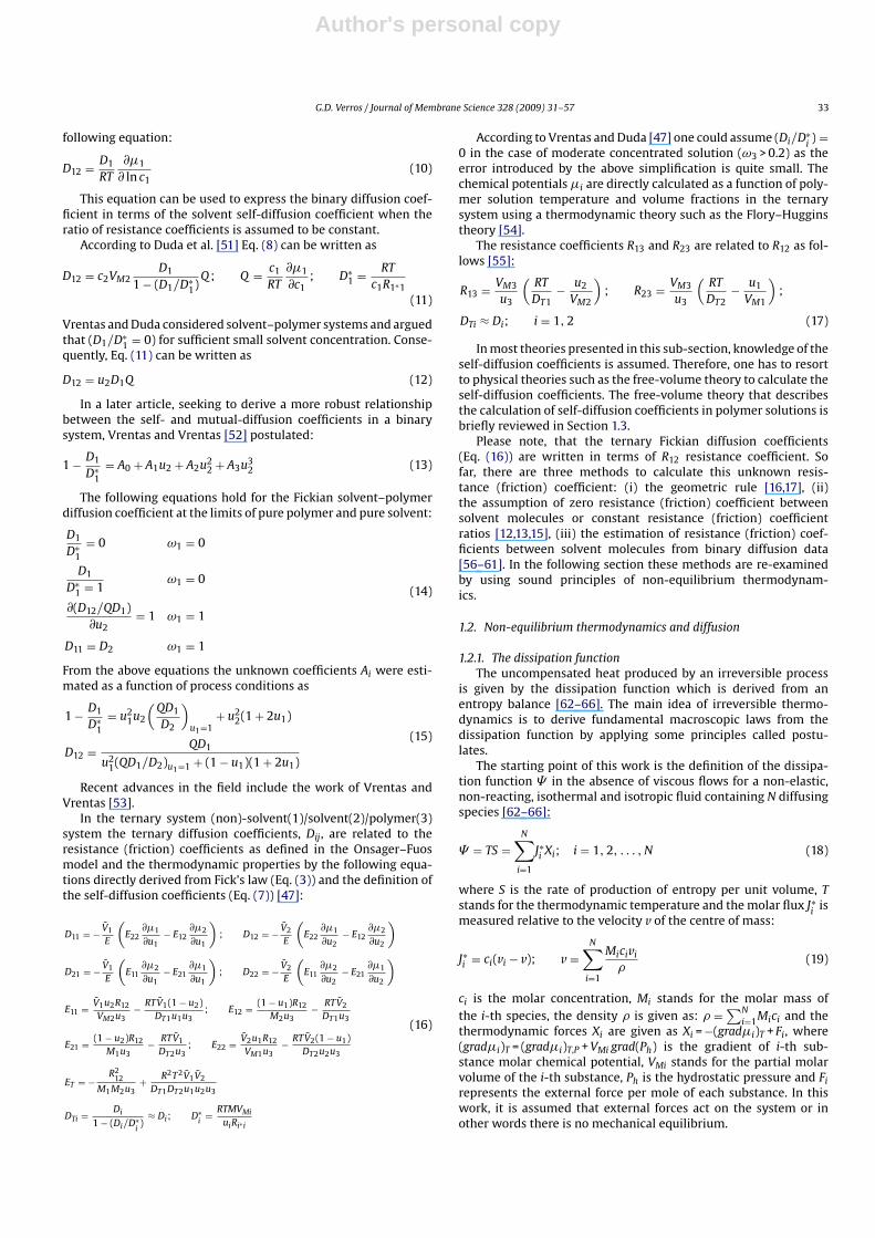
0 in the case of moderate concentrated solution (ω3 > 0.2) as theerror introduced by the above simplification is quite small. Thechemical potentials �i are directly calculated as a function of poly-mer solution temperature and volume fractions in the ternarysystem using a thermodynamic theory such as the Flory–Hugginstheory [54].

The resistance coefficients R13 and R23 are related to R12 as fol-lows [55]:

R13 = VM3

u3

(RT

DT1− u2

VM2

); R23 = VM3

u3

(RT

DT2− u1

VM1

);

DTi ≈ Di; i = 1, 2 (17)

In most theories presented in this sub-section, knowledge of theself-diffusion coefficients is assumed. Therefore, one has to resortto physical theories such as the free-volume theory to calculate theself-diffusion coefficients. The free-volume theory that describesthe calculation of self-diffusion coefficients in polymer solutions isbriefly reviewed in Section 1.3.

Please note, that the ternary Fickian diffusion coefficients(Eq. (16)) are written in terms of R12 resistance coefficient. Sofar, there are three methods to calculate this unknown resis-tance (friction) coefficient: (i) the geometric rule [16,17], (ii)the assumption of zero resistance (friction) coefficient betweensolvent molecules or constant resistance (friction) coefficientratios [12,13,15], (iii) the estimation of resistance (friction) coef-ficients between solvent molecules from binary diffusion data[56–61]. In the following section these methods are re-examinedby using sound principles of non-equilibrium thermodynam-ics.

1.2. Non-equilibrium thermodynamics and diffusion

1.2.1. The dissipation functionThe uncompensated heat produced by an irreversible process

is given by the dissipation function which is derived from anentropy balance [62–66]. The main idea of irreversible thermo-dynamics is to derive fundamental macroscopic laws from thedissipation function by applying some principles called postu-lates.

The starting point of this work is the definition of the dissipa-tion function � in the absence of viscous flows for a non-elastic,non-reacting, isothermal and isotropic fluid containing N diffusingspecies [62–66]:

� = TS =N∑

i=1

J∗i Xi; i = 1, 2, . . . , N (18)

where S is the rate of production of entropy per unit volume, Tstands for the thermodynamic temperature and the molar flux J∗

iis

measured relative to the velocity v of the centre of mass:

J∗i = ci(vi − v); v =N∑

i=1

Micivi

�(19)

ci is the molar concentration, Mi stands for the molar mass ofthe i-th species, the density � is given as: � =

∑Ni=1Mici and the

thermodynamic forces Xi are given as Xi = −(grad�i)T + Fi, where(grad�i)T = (grad�i)T,P + VMi grad(Ph) is the gradient of i-th sub-stance molar chemical potential, VMi stands for the partial molarvolume of the i-th substance, Ph is the hydrostatic pressure and Firepresents the external force per mole of each substance. In thiswork, it is assumed that external forces act on the system or inother words there is no mechanical equilibrium.

Author's personal copy

34 G.D. Verros / Journal of Membrane Science 328 (2009) 31–57

At this point, it is necessary to introduce new fluxes, definedrelative to an arbitrary reference velocity v /= :

J /=i

= ci(vi − v /= ); v /= =N∑

i=1

wivi (20)

where wi are weighting factors whose sum is unity:∑N

i=1wi = 1

Please note, that the following equation holds for fluxes J /=i

,directly derived from Eq. (20):

N∑i=1

wiJ/=

i/ci = 0 (21)

Schmitt and Graig [67] have shown that if the transformed

thermodynamic forces X ′i= Xi + Mi

(grad(Ph) −

∑Nj=1cjFj

)/� are

introduced in the dissipation function Eq. (18), then the dissipa-tion function is invariant under the transformation to the new setof fluxes as well as to the thermodynamic forces:

� =N∑

i=1

J /=i

X ′i (22)

The importance of this analysis is shown in Section 1.2.2.

1.2.2. Non-equilibrium thermodynamics postulatesNon-equilibrium thermodynamics is based on three inde-

pendent postulates above and beyond those of equilibriumthermodynamics [62–66]:

1. All the fluxes (Ji) in the system may be written as linear relationsinvolving all the thermodynamic forces, X ′

i. (linearity postulate,

X ′i=∑N

j=1R /=ij

J /=j

; i = 1, 2, . . . , N) R /=ij

represents the resis-tance (friction) coefficients.

2. The equilibrium thermodynamic relations apply to systems thatare not in equilibrium, provided that the gradients are not toolarge (quasi-equilibrium postulate). More specifically this pos-tulate states that equilibrium thermodynamic relations suchas the Gibbs–Duhem equation, can be applied to the system.Schmitt and Graig [67] have shown that if the transformed

thermodynamic forces X ′i= Xi + Mi

(grad(Ph) −

∑Nj=1cjFj

)/�

introduced in the previous section are applied along withthe Gibbs–Duhem equation

∑Ni=1ci(grad�i)T,P = 0 the following

equation is derived:

N∑i=1

ciX′i = 0 (23)

Following most researchers in the field, as reviewed by Tyrrelland Harris [21], the resistance coefficients (see Linearity Postu-late) are introduced into the Gibbs–Duhem equation (Eq. (23))and the following equation is derived by assuming that the resis-tance coefficients are uniquely defined and independent of theflux reference velocity (v /= ):

N∑k=1

ckX ′k =

N∑k=1

ck

N∑i=1

R /=ki

J /=i

=N∑

i=1

J /=i

N∑k=1

R /=ki

ck = 0

orN∑

k=1

ckR /=ki

= 0; i = 1, 2, . . . , N (24)

The above equation was derived for the first time by Onsager[68]. In his view the above equation has a clear physical mean-

ing: if the solution container is moved there is no dissipation ofenergy caused in the solution.

Miller [69] has shown that the Onsager–Fuos model (Eq. (3))for diffusion can be directly derived by applying the linearitypostulate along with the Gibbs–Duhem equation (Eq. (24)).

3. In the absence of magnetic fields and assuming linearly indepen-dent fluxes or thermodynamic forces the matrix of coefficientsin the flux-force relations is symmetrical. This postulate isknown as Onsager reciprocal relations (ORR): R /=

ij= R /=

ji.

Onsager derived these relations in the case of heat transferin 1931 [44,45]. It is worth noting that Onsager did not use aparticular molecular model. As a consequence the results and lim-itations of the theory are valid for all materials, so the theory canbe related to a continuum theory [62–66]. Onsager [44,45] usedthe principle of microscopic reversibility by applying the invari-ance of the equations of motion for atoms and molecules withrespect to time reversal (the transformation t → −t). This meansthat the mechanical equations of the motion (classical as well asquantum mechanical) of particles are symmetrical with respectto time. In other words, the particles retrace their former pathsif all velocities are reversed. Onsager also made a principal deci-sion: the transition from molecular reversibility to microscopicreversibility can be made. Casimir further developed this theory[70].

In the literature there appear to be two groups of derivationsof Onsager reciprocal relations. In the first of these, it is assumedthat the macroscopic laws of motion hold for the averages of themacroscopic coordinates (such as temperature gradient, concentra-tion gradient, etc.) even if their values are microscopic. The secondgroup assumes a definite statistical law for the path representingthe system in phase space [71].

Although there is experimental evidence for the validity of theORR [72,73], as was noticed by Prigogine and Kondepudi [74], in arecent review the theoretical basis of ORR requires careful consid-eration. Moreover, doubts about ORR [75,76] have been raised inthe literature.

In our previous work [77], it was shown by following Lorimer’swork [78,79] that ORR are necessarily fulfilled in the case ofmulti-component diffusion, independently of the flux referencesystem. Moreover, ORR for multi-component diffusion are neces-sarily fulfilled when the quasi equilibrium postulate (Gibbs–Duhemequation) is applied [77]. It is also shown that the phenomenolog-ical coefficients in this case are uniquely defined [77]. Alternativeproof for this statement was given by Miller [69]. Extension of thisproof to simultaneous heat and mass transfer is given elsewhere[80].

1.2.3. Multi-component diffusion theory for polymer solutionsFor simplicity, in the remainder of this work the superscript /=

is omitted in the flux and resistance (friction) coefficients notation.In Eq. (16) the Fickain diffusion coefficients Dij are related not onlyto self-diffusion coefficients but also to the R12 resistance (friction)coefficient which must be determined. This could be achieved byassuming a constant value for R12 estimated from the binary dif-fusion coefficient data for the solvent(1)–solvent(2) system at thelimit of zero polymer concentration [56–61] or one could simplyassume R12 = 0 [12]. Alternatively, other approaches such as thegeometric rule [16,17] or the assumption of constant resistancecoefficient ratios [12,13] could be applied.

By using the relationship between partial molar volumes(∑Ni=1ciVMi = 1

)along with Gibbs–Duhem equations and the geo-

metric rule (R2ij

= RiiRjj), one directly derives the following equation

Author's personal copy

G.D. Verros / Journal of Membrane Science 328 (2009) 31–57 35

in the case of constant resistance coefficients ratios [17]:

Rij/Rkj = VMi/VMk = V̄i

V̄k

Mi

Mk(25)

This equation also proposed by Alsoy and Duda [12], simulta-neously satisfies the Onsager reciprocal condition as well as theGibbs–Duhem relation along with the concept of constant resis-tance coefficient ratio. However, the constant resistance coefficientratios assumption leads to either additional equations for Fickiandiffusion coefficients or to a restriction on the values of the self-diffusion coefficients [81].

The geometric rule (R2ij

= RiiRjj) is not a new idea [21,82]. The geo-metric rule has been widely used to model industrial processes [16].The geometric rule satisfies simultaneously the non-equilibriumpostulates and the uniqueness criterion of the resistance coeffi-cients for diffusion. By applying the geometric rule to the linearitypostulate a system of N − 1 independent equations is obtainedand the quasi equilibrium postulate (Gibbs–Duhem theorem) isreduced to a single equation:

X ′i =

√Rii

(N∑

k=1

√RkkJk

); i = 1, 2, . . . , N − 1 (26)

N∑i=1

ci

√Rii = 0 (27)

The above system consists of N equations with N unknowns(Rii) which are uniquely defined. By introducing the modifiedGibbs–Duhem equation (Eq. (24)) into the linearity postulate thefollowing equation is derived:

Rii = X ′2i∑N

i=1JiX′i

; i = 1, 2, . . . , N (28)

The denominator in Eq. (28) is the dissipation function (Eq. (22))which is uniquely defined [62–66]. Therefore, the resistance coef-ficients are uniquely defined.

The idea of the geometric rule has been proposed by Priceand Romdhane [16] and it has been widely used to modelindustrial processes [16]. The geometric rule along with the non-equilibrium thermodynamics postulates could be used to defineall the resistance coefficients if the low molecular weight sub-stances self-diffusion coefficients are known. The geometric rulecombined with the Gibbs–Duhem theorem results in a simple alge-braic system which is directly solved to calculate the resistance andconsequently Dij in terms of the process conditions [17]:

c1R11 + c2R12 + c3R13 = 0; R212 = R11R22;

R13

R23=√

R11

R22

(29)

Alternatively, one could write:

c1R11 + c2R12 + c3R13 = 0; c1R12 + c2R22 + c3R23 = 0 (30)

R212 = R11R22 (31)

A detailed comparison between the predictions of these the-ories for the systems formamide/acetone/cellulose acetate andwater/acetone/cellulose acetate is given in Section 4 of this work.

1.3. Free-volume theory

The importance of the accurate prediction of diffusion coef-ficients as a function of the temperature and concentration wasthe motivation for many researchers in industry and academia to

develop the free-volume theory. According to Vrentas and Duda[18,19] the first theoretical basis for a free-volume theory of trans-port was provided by Cohen and Turnbull [83], who consideredmolecular transport in a liquid of hard spheres and related theself-diffusion coefficient to the free volume of the system. Differ-ent versions of the free-volume theory of diffusion have also beenproposed by Fujita [84], Vrentas and Duda [18,19], Paul [85]. Theconceptual differences between the various free volume theorieswere examined by many researchers in the field [18,19,86–88] andit was shown that the most accurate free-volume theory for the dif-fusion in polymer solutions was the Vrentas–Duda theory [18,19].

In the Vrentas–Duda free-volume theory, the total volume of asystem is assumed to be comprised of two parts: the volume occu-pied by the molecules, known as critical volume, and the volumethat is left unoccupied, known as free volume. The free volume inthe system can be of two types: interstitial free volume and hole freevolume. The interstitial free volume has high activation energy forbeing redistributed through the system. The interstitial free volumeis the major component of the total free volume of the system whenthe system is below its glass transition temperature. At tempera-tures above the glass transition temperature of the system there isan increase in the free volume of the system and this increase ismainly an increase in the hole free volume. The hole free volumeredistributes more easily to allow solvent molecules to diffuse.

The main idea of this theory is that a molecular mixture con-tains dynamic ‘holes’ of various sizes. If a ‘hole’ has a volumeequal to or larger than that of a solvent molecule or a polymer-jumping unit, then diffusion can occur. The polymer-jumping unitis defined to be the effective part of the polymer chain that takespart in the diffusive process. The diffusive process involves the mov-ing of a molecule into an adjacent hole if the hole is big enoughand the molecule possesses sufficient energy to overcome theactivation barrier. Therefore the hole free volume controls the dif-fusion process. This sub-section closely follows the original workof Vrentas–Duda [18,19]. The Vrentas–Duda theory is based on thefollowing concepts:

(1) The specific occupied volume of a liquid V̂0 is defined to be thespecific volume V̂(0) of the equilibrium liquid at 0 K. Hence, thespecific free volume V̂F is given by

V̂F = V̂ − V̂0 = V̂ − V̂(0) (32)

where V̂ is the specific volume of the equilibrium liquid struc-ture at any temperature T. Even though it is not possible tomeasure V̂(0) directly, this quantity can be estimated by groupcontribution methods.

(2) The specific occupied volume V̂0 is assumed to be independentof molecular weight for polymeric liquids.

(3) As the temperature is increased from 0 K, the increase in volumeis realized partly by the homogeneous expansion of the mate-rial and partly by the formation of holes or vacancies whichare distributed discontinuously throughout the material at anyinstant. Therefore the following relation holds for the specificfree volume V̂F of the system:

V̂F = V̂FI + V̂FH (33)

where V̂FI is the specific interstitial free volume and V̂FH is thespecific critical hole free volume.

(4) The thermal expansion coefficient for the sum of the specificoccupied volume and the specific interstitial free volume isgiven by the following equation:

1

V̂F0 + V̂0

[∂(V̂F0 + V̂0)

∂T

]P

= ac (34)

Author's personal copy

36 G.D. Verros / Journal of Membrane Science 328 (2009) 31–57

which yields the following expression upon integration:

V̂F0 + V̂(0) = V̂(0) exp

⎧⎨⎩

T∫0

acdT

⎫⎬⎭ (35)

Since the free-volume theory is usually applied at temper-atures significantly above 0 K, it is convenient to utilize thefollowing alternative expression for V̂FI + V̂(0) in terms of themeasured glass transition temperature of the material TG:

V̂F0 + V̂(0) = [VF (TG) + V̂(0)] exp

{∫ T

TG

acdT

}(36)

(5) It is assumed that ac, for polymeric liquids is independent ofmolecular weight; this should be a reasonable assumption formolecular weights of ordinary interest.

(6) For a binary mixture, Vrentas and Duda [18,19] assumed additiv-ity of the volumes formed from the sum of the specific occupiedvolume and the specific interstitial free volume. Thus, it followsthat

(V̂FI + V̂0)M = V̂01 (0)ω1 exp

{∫ T

0

ac1dT

}

+ V̂02 (0)ω2 exp

{∫ T

0

ac2dT

}(37)

where (V̂FI + V̂0)M represents the sum of the specific occupiedvolume and the specific interstitial free volume of the mixture,ωi is the mass fraction of component i, and V̂0

1 is the specificvolume of pure component i at 0 K. Consequently, the followingequation holds for a mixture:

(V̂FI + V̂0

)M

= ω1[VFI1(TG1) + V̂0

1 (0)]

exp

{∫ T

0

ac1dT

}

+ ω2[VFI2(TG2) + V̂0

2 (0)]

exp

{∫ T

0

ac2dT

}(38)

(7) The thermal expansion coefficients for the sum of specificoccupied and specific interstitial free volumes, acl and ac2 areassumed to be independent of temperature. Therefore, the spe-cific hole free volume for the binary mixture can be calculatedfrom the properties of the pure components and from measuredor predicted values for the specific volume V̄M of the mixtureby using the following equation:

V̂FH = V̄M − (V̂FI + V̂0)M (39)

Following previous work, Vrentas and Duda wrote the followingexpression for the self-diffusion coefficient of a one-component,simple liquid system:

D1 = D01 exp

{�V̄∗

1VFHM

}exp

{− E

RT

}(40)

Here, D1 is the self-diffusion coefficient of component 1, VMFH isthe average hole free volume per molecule in the liquid; is the crit-ical local hole free-volume required for a molecule of species oneto jump to a new position; � is an overlap factor which is intro-duced because the same free volume is available to more than onemolecule; and E is the critical energy a molecule must obtain inorder to overcome the attractive forces holding it to its neighbors.For temperatures near the measured glass transition temperatureof a liquid, the specific hole free volume is relatively small and the

self-diffusion process is free-volume dominated. Hence, in the tem-perature interval, say, from TG to TG + 100 ◦C it is possible to absorbthe E term into the pre-exponential factor and write Eq. (40) as

D1 = D01 exp

{�V̄∗

1VMFH

}(41)

By introducing the assumption stated above, namely that thenature of the molecular species in a binary mixture in no way influ-ences the random distribution of hole free volume, Vrentas andDuda derived modified versions of Eqs. (40) and (41) for the self-diffusion coefficients of solvent and polymer in a binary mixture.This modification is based simply on defining the average hole freevolume per molecule as the total hole free volume of the systemdivided by the number of molecules of solvent plus the numberof jumping units of the polymer. Hence, in a mixture of a simpleliquid and a polymeric liquid, it can easily be shown that the fol-lowing expressions describe the concentration dependence of theself-diffusion coefficients:

D1 = D01 exp

{�(ω1V∗

1 + ω2�V∗2 )

VFH

}(42)

Here, VFH is the average hole free volume per kg of mixture, V∗i

isthe specific critical hole free volume of i-th component, and thequantity � is defined by the equation:

� = V̄∗1/V̄∗

2 = V∗1M1/V∗

2Mj (43)

where V∗1 is the critical volume of solvent per mole of solvent, V∗

2is the critical volume of jumping units per mole of jumping units,M1 is the molecular weight of the solvent, and Mj is the molecularweight of a jumping unit. It is reasonable to expect that the criticalamount of local hole free volume per gram necessary for a jump totake place is approximately equal to the specific occupied volumeof the liquid and so Vrentas and Duda stated:

V∗1 = V̄0

1 (0); V∗2 = V̄0

2 (0) (44)

The thermal expansion coefficients of the solvent and polymer,ai = (1/V̄0

i)((∂V̄0

i/∂T))

p, are approximated by average values in the

temperature range under consideration. Moreover, for all expan-sion coefficients utilized in the theory and for the temperatureintervals of interest, approximations of the type:

exp{

˛1(T − TG)}

= 1 + ˛1(T − TG) (45)

are assumed to be sufficiently accurate. By using Eqs. (38)–(41) andEq. (45) it can be directly shown that that the specific hole freevolume of the solvent (V̂FH1) is given by the following equations:

V̂FH1 = K11(K21 − T − TG1); f GH1

= V̂FH1(TG1)

V̄01 (TG1)

K11 = V̄01 (TG1)[a1 − (1 − f G

H1)ac1]; K21 =

f GH1

[a1 − (1 − f GH1

)ac1]

(46)

Here, a1 and ac1 are to be regarded as appropriate average val-ues over the temperature interval of interest. An equivalent set ofequations can be derived for the polymer, component 2, involvingconstants K12 and K22.

Regarding the estimation of the parameters, the two critical vol-umes, V∗

1 and V∗2 can be estimated as the specific volumes of the

solvent and polymer at 0 K. Molar volumes of the solvent and poly-mer at 0 K can be estimated using group contribution methods [89].The polymer parameters (K22, K12/�) can be estimated from purepolymer viscosity data. For pure polymers, the temperature depen-dencies of the viscosity p(T) are usually expressed in terms of the

Author's personal copy

G.D. Verros / Journal of Membrane Science 328 (2009) 31–57 37

Williams–Landel–Ferry [90] equation:

ln

(p(T2)p(TG2)

)= −CWLF

12 (T − TG2)

CWLF22 + T − TG2

(47)

The Williams–Landel–Ferry [90] equation parameters have beentabulated for a large number of polymers. From the above equationit follows that:

K22 = CWLF12 ;

K12

�= V∗

2

2.303CWLF12 CWLF

22

(48)

The parameters K11 and K21 – TG1 can be estimated from thepure solvent viscosity data. More specifically by Adopting Doolit-tle’s expression [91] and using the nomenclature of Vrentas andDuda leads to Eq. (49) for the solvent viscosity:

ln s = ln B + �V∗1/K11

K21 − TG1(49)

Hence, K11 and K21 − TGl can be determined from a non-linearregression of Eq. (49) by using pure solvent viscosity-temperaturedata. In addition, D0 and E can be estimated by combining the Dul-lien equation [92] for the self-diffusion coefficient of pure solventswith the Vrentas–Duda free-volume equation evaluated in the limitof pure solvents. Thus

ln

(0.124 × 10−16V2/3

c RT

s(T)M1V̂1

)= ln D0 − E(ω1 → 1)

RT− �V∗

1/K11

K21 − TG1(50)

where s(T) represents the solvent viscosity at temperature T andVc stands for the critical molar volume of the solvent, respectively.This analysis leaves only the parameter � to be estimated. Ju et al. [9]assumed that the size of the polymer-jumping unit is independentof the solvent and proposed a linear relationship between � and thesolvent molar volume at 0 K, VM1(0), so that:

� = AF VM1(0) (51)

where AF = 1/V̄∗2j

is a constant which has been determined from thepolymer/solvent diffusion data. Once AF is known for a particularpolymer, the value of AF for any solvent in that polymer can beestimated if the solvent moves as a single unit. Zielinski and Duda[93], Hong [94], Vrentas et al. [10], Wang et al. [95] extended furtherthe predictive capabilities of this theory. Although a more advancedversion of free-volume theory is available [95], the version of thefree-volume theory presented in this section could be consideredsufficient for the purpose of this work.

The Vrentas–Duda theory was extended to multi-componentcomponent mixtures by Ling et al. [55]. According to these workersthe self-diffusion coefficient Di of the i-th component in the ternarysolution and is given as follows:

D1 = D01 exp

(−(ω1V∗

1 + ω2V∗2�13/�23 + ω3V∗

3�13)

VFH/�

)(52)

D2 = D02 exp

(−(ω1V∗

1�23/�13 + ω2V∗2 + ω3V∗

3�23)

VFH/�

)(53)

VFH

�=

3∑i=1

K1i

�(K2i − TGi + T)ωi (54)

D0i is a pro-exponential factor, VFH is the average hole free volumeper kg of the solution and � is an overlap factor, which is intro-duced, because the same free volume is available to more than onemolecule. V∗

iis the specific critical hole free volume of the i-th com-

ponent required for a diffusion jump and �i3 represents the ratio ofthe critical molar volume of the jumping unit of i-th-solvent to that

of the polymer. K1i and K2i are free volume parameters for the i-thcomponent and TGi is the glass transition temperature. In the aboveequations ωi represents the weight fraction of the i-th substance.

In the previous sections the fundamental aspects of diffusion inpolymer solutions were reviewed. It was shown that the Fickiandiffusion coefficients in polymer solutions are written in terms ofthe self-diffusion coefficients as calculated by the free-volume the-ory. The free-volume theory parameters are well established andthey could be directly estimated from independent experiments ortheoretical considerations. Alternatively, combined methods suchas the solvent evaporation method could be used to determinethe unknown parameters of the free-volume theory such as the �parameter (see Eqs. (42) and (52)–(54)). This could be achieved byusing advanced modeling combined with simple laboratory exper-iments. This is the task of the solvent evaporation method. The aimof this work is to review recent advances in the field of the solventevaporation method in Section 2.

2. The solvent evaporation method

The solvent evaporation method combines simple laboratoryexperiments with advanced modeling, in order to get accurate esti-mates of the diffusion coefficients. In particular, the laboratoryexperiments consist of gravimetric measurement of the solventevaporation rate from appropriate cast polymer–solvent films. Themeasured solvent evaporation rate is compared with model pre-dictions, in order to estimate the unknown parameters of theVrentas–Duda equation [18,19].

This idea was proposed by Ataka and Sasaki [96]. However,only the implementation of robust numerical methods such asGalerkin finite elements, allow its realization by studying thesolvent evaporation process in the general framework of compu-tational transport phenomena. Undeniably, Price et al. [97] werethe first who got accurate estimates of the diffusion coefficients byfitting drying rate in order to optimize the performance of indus-trial dryers. Verros and Malamataris [98–100], further applied thismethod to other systems. Finally, Doumenc and Guerrier [101]examined the computational aspects of the solvent evaporationmethod.

In this method, the evaporation process is studied as a one-dimensional numerical experiment utilizing the Galerkin finiteelement method. This numerical technique provides simultaneoussolution of the model equations and yields the diffusion coefficientsof the solvent in the polymer over a wide range of temperatureand composition by comparing model predictions with gravimetricdata.

In the next sections, the evaporation process is described andthe governing equations of the solvent evaporation process alongwith the appropriate initial and boundary conditions for binaryand ternary solutions are given. The finite element formulation isdescribed in full detail in Section 2.4.

2.1. Process description

According to this method, the solvent evaporation rate is mea-sured gravimetrically, using the experimental set-up of Fig. 1.

The thin cast liquid films (after their preparation on glass slides)are transferred to a microbalance, which is connected with a per-sonal computer for data acquisition. To prevent heat exchangebetween the glass slides and the microbalance pan, the glass slidesare placed on an insulating block resting upon the microbalancepan (Fig. 1). The microbalance was exposed to the ambient air, sothat accumulation of solvent(s) vapor in the vicinity of the equip-ment is avoided and zero solvent concentration in the bulk of gasphase is ensured.

Author's personal copy

38 G.D. Verros / Journal of Membrane Science 328 (2009) 31–57

Fig. 1. Schematic representation of the experimental set up for the solvent evapo-ration measurement.

Our system consists of a liquid layer resting upon an imper-meable solid support exposed to a gas phase of temperature T0.The liquid layer is the solvent(s)–polymer solution and has an ini-tial thickness L0. The support is a flat, horizontal glass plate withconstant thickness Lsup, allowing heat exchange with the poly-mer solution. Prior to time zero, the polymer solution is assumedto have a constant initial solvent concentration everywhere inits mass and the whole system has the same initial tempera-ture T0. At time t = 0, a liquid–gas interface is suddenly createdby exposing the polymer solution to the gas phase. The volatilesolvent(s) begins to evaporate resulting in a downward motionof the liquid–gas interface. As the solvent(s) at the surface evap-orates, the gas–liquid interface is cooled. From an engineeringpoint of view this is a coupled heat and mass transfer processwith a moving boundary. Since diffusion is much slower thanthe relaxation mechanisms of the polymer chains in the solu-tion, we assume pure Fickian diffusion [12,13,15–17,47,48,102,103].Additionally, due to the relatively small initial thickness of thepolymer solution (order of �m) compared to the width andlength (order of cm), the process is considered as 1-dim model[12,13,15–17,47,48,102,103].

2.2. Model equations for binary systems

The dimensionless governing equations, which define the evap-oration model for the binary systems are [98,99]:

∂u1

∂= ∂

∂

(C0

∂u1

∂

); C0 = D/D0; 0 < < s (55)

C1∂�

∂= ∂

∂

(C2

∂�

∂

); C1 = �Cp/�0Cp0; C2 = k/D0�0Cp0;

0 < < s (56)

C3∂�sup

∂= ∂

∂

(C4

∂�sup

∂

); C3 = �supCpsup/�0Cp0;

C4 = ksup/�0Cp0D0; Lsup/L0 < < 0 (57)

Eqs. (55)–(57) represent the conservation of mass and energy inthe binary polymer solution and the support, respectively, assum-ing one-dimensional Fickian diffusion. u1 is the acetone volumefraction, = z/L0 is the dimensionless space coordinate; = D0t/L0

2

is dimensionless time; � = T/T0 is dimensionless temperature ands = L(t)/L0 is the dimensionless position of the moving boundary. Trepresents the temperature, t denotes time and D0 is a scaling factorhaving the units of diffusion coefficient. D12 is the mutual diffusioncoefficient. Equations for D12 were presented and discussed in Part1. �, Cp and k represents density, specific heat capacity and ther-mal conductivity of the polymer solution, respectively. Cp0, �0 arescaling factors having units of specific heat capacity and density,respectively. Subscript ‘sup’ denotes properties and variables of thesupport.

Initial and boundary conditions for the diffusion equation:

u1 = u10; = 0 (58)

C0∂u1/∂ = C5(xint − x∞); C5 = −L0kGP/V̄1/D0; = s

(59)

∂u1/∂ = 0; = 0 (60)

Eq. (59) is a mass balance at the moving interface and Eq. (60) speci-fies zero mass flux at the glass plate. xint and x∞ are the solvent molefraction at the liquid layer–gas phase interface and far away fromthe interface, respectively. P is the total pressure, V̄1 denotes the sol-vent partial specific volume and kG is the mass transfer coefficientin the gas phase.

Initial and boundary conditions for the energy equations:

� = �sup = 1; t = 0 (61)

C2∂�/∂ = C6(� − 1) + C7(1 − �4int) − C8(xs − x∞);

C6 = L0h/D0�0Cp0

C7 = L0ε T30 /D0�0Cp0; C8 = (�H)kGPL0/(T0D0�0Cp0);

= s

(62)

C4∂�sup/∂ = C2∂�/∂; = 0 (63)

∂�sup/∂ = 0; = −Lsup/L0 (64)

Eq. (62) is an energy balance at the moving interface, equatingthe heat conduction to the polymer solution with free convectionheat transfer, radiant heat transfer from the ambient air and latentheat loss due to acetone evaporation. Eq. (63) implies continuityof temperature and heat flux at the glass plate–polymer solutioninterface, while Eq. (64) implies perfect insulation of the glass sup-port lower surface. �int denotes the dimensionless temperature ofthe liquid–gas interface, h is the heat transfer coefficient, ε is theemissivity of the polymer solution, denotes the Stefan–Boltzmanconstant and �H is the acetone latent heat of vaporization.

Finally, the instantaneous dimensionless solution thickness s isobtained from the conservation of the polymer mass:∫ s

0

(1 − u1)d =∫ 1

0

(1 − u10)dn (65)

Eq. (65) is the definition of the instantaneous position of the mov-ing boundary and is solved simultaneously with the governingEqs. (55)–(57) along with the boundary conditions (58)–(64) asexplained in detail in the section finite element formulation.

Author's personal copy

G.D. Verros / Journal of Membrane Science 328 (2009) 31–57 39

2.3. Model equations for ternary systems

The dimensionless model equations describing the conservationof energy in a one phase ternary system and the support are identi-cal to the equations for the binary system presented in the previoussection. The dimensionless equations describing the conservationof mass in a ternary system are written as follows [17,61,100]:

∂u1

∂= ∂

∂

(C1T

∂u1

∂

)+ ∂

∂

(C2T

∂u2

∂

); = z/L0;

= D0t/L20; C1T = D11/D0; C2T = (V̄1/V̄2)D12/D0;

0 < < s = L(t)/L0 (66)

∂u2

∂= ∂

∂

(C3T

∂u1

∂

)+ ∂

∂

(C4T

∂u2

∂

); C3T =(V̄2/V̄1)D21/D0;

C4T = D22/D0; 0 < < s (67)

In this work subscript 1 refers to solvent A, 2 denotes solventB and subscript 3 represents the polymer. Dij are the appropri-ate phenomenological diffusion coefficients for the ternary system.Equations for Dij were presented in Section 1.

Initial and boundary conditions for the diffusion equations:

u1 = u10; u2 = u20; = 0 (68)

C1T ∂u1/∂ + C2T ∂u2/∂ = C9; C9 = −L0jA,intV̄1/D0; = s

(69)

C3T ∂u1/∂ + C4T ∂u2/∂ = C10; C10 = −L0jB,intV̄2/D0; = s

(70)

∂u1/∂ = 0; ∂u2/∂ = 0; = 0 (71)

Eq. (68) gives the initial concentration for the solvents A and B. Eqs.(69) and (70) are mass balances at the moving interface and Eq.(71) specifies zero mass flux at the glass plate. jA,int and jB,int arethe mass flux of the substance A and B, at the gas–liquid interface.The above fluxes also appear in the boundary equation for the heattransfer at the interface of the gas-phase–polymer solution (termdescribing the latent heat of evaporation).

The conservation of the polymer mass gives the following equa-tion for position s of the moving boundary:∫ s

0

(1 − u1 − u2)d =∫ 1

0

(1 − u10 − u20)d (72)

An alternative equation is obtained from the following equa-tion between the mass fluxes Ji in a N-component system wherediffusion takes place [49]:

N∑i=1

V̄iji = 0 (73)

Eq. (73) is essentially the conservation of mass in multi-componentdiffusion and it is valid at any point of the computational domain.At the gas–liquid interface of the ternary system the mass fluxesare given as follows:

j1 = jA,int; j2 = jB,int; j3 = �3dL(t)/dt; �i = ui/V̄i (74)

By combining (74) with (73) and dedimensionlizing we obtainthe following differential equation which defines the instantaneous

dimensionless solution thickness s = L(t)/L0 [61,100]:

u3ds/d = C9 + C10; = 0, s = 1 (75)

Eq. (75) defines the instantaneous position of the moving boundaryin terms of the polymer volume fraction u3 = 1 − u1 − u2 Eq. (75) isa differential mass balance and Eq. (72) is the integral mass balancefor the polymer, since only the solvents evaporate from the polymersolution. A comparison of the computational efficiency by solvingEq. (72) or (75) is given in Section 2.4. These equations are solvedby the Galerkin finite element method along with the governingequations of the model to calculate the concentration profiles ofsolvents along with the temperature of the solution and the supportand position of the moving boundary as a function of time. TheGFEM is described in Section 2.4.

2.4. Finite element formulation for ternary systems

The computational domain is discretized in 70 finite elements.The unknown volume fractions, uj and the temperature � areexpanded in terms of quadratic Galerkin basis functions, ϕi as

uj =3∑

i=1

uijϕ

i j = 1, 2; � =3∑

i=1

�iϕi (76)

In the nodes of support, the energy equation is evaluated, theonly unknown is the temperature and this part of the domain isfixed. In the polymer solution both the energy and mass equationsare evaluated, each node has temperature and volume fractions asunknowns and this part of the domain deforms according to themotion of the moving boundary. Finally, the boundary position, s,is added as unknown at the last node of the computational domain.The governing equations weighted integrally with the basis func-tions resulted in the following mass Ri

M , energy RiE and kinematic

RNK residuals:

RiM1 =

∫ s

0

[∂u1

∂− ∂

∂

(C1T

∂u1

∂

)− ∂

∂

(C2T

∂u2

∂

)]ϕid (77)

RiM2 =

∫ s

0

[∂u2

∂− ∂

∂

(C3T

∂u1

∂

)+ ∂

∂

(C4T

∂u2

∂

)]ϕid (78)

RiE,sol =

∫ s

0

[C1

∂�

∂− ∂

∂

(C2

∂�

∂

)]ϕid (79)

RiE,sup =

∫ 0

−L/Lsup

[C3

∂�sup

∂− ∂

∂

(C4

∂�sup

∂

)]ϕid (80)

RNK = u3ds/d − C9 − C10 or RN

K

=∫ s

0

(1 − u1 − u2)d −∫ 1

0

(1 − u10 − u20)d (81)

In order to account for the moving boundary, the total timederivatives for volume fraction and temperature were calculated,introducing convective terms in the governing equations [104,105]:

dui/d = ∂ui/∂ + (d/d)(∂ui/∂); i = 1, 2 (82)

d�/d = ∂�/∂ + (d/d)(∂�/∂) (83)

By combining the above equations with the weighted residuals(77)–(79) we obtain the following equations:

RiM1 =

∫ s

0

[du1

d−d

d

∂u1

∂− ∂

∂

(C1T

∂u1

∂

)− ∂

∂

(C2T

∂u2

∂

)]ϕid

(84)

Author's personal copy

40 G.D. Verros / Journal of Membrane Science 328 (2009) 31–57

RiM2 =

∫ s

0

[du2

d−d

d

∂u2

∂− ∂

∂

(C3T

∂u1

∂

)− ∂

∂

(C4T

∂u2

∂

)]ϕid

(85)

RiE,sol =

∫ s

0

[C1

d�

d− d

dC1

∂�

∂− ∂

∂

(C2

∂�

∂

)]ϕid (86)

In order to decrease the order of differentiation and project theNeuman (natural) boundary conditions of the problem, integrationby parts (divergence theorem in one-dimension) is applied and theweighted residuals become:

RiM1 =

∫ s

0

[du1

dϕi − d

d

∂u1

∂ϕi + ∂ϕi

∂

(C1T

∂u1

∂

)

+∂ϕi

∂

(C2T

∂u2

∂

)]d −

(C1T

∂u1

∂+ C2T

∂u2

∂

)ϕi

∣∣∣∣=s

=0

(87)

RiM2 =

∫ s

0

[du2

dϕi − d

d

∂u2

∂ϕi + ∂ϕi

∂

(C3T

∂u1

∂

)

+∂ϕi

∂

(C4T

∂u2

∂

)]d −

(C3T

∂u1

∂+ C4T

∂u2

∂

)ϕi

∣∣∣∣=s

=0

(88)

RiE,sol =

∫ s

0

[C1

d�

dϕi − d

d

∂�

∂C1ϕi + ∂ϕi

∂

(C2

∂�

∂

)]d

− C2∂�

∂ϕi

∣∣∣∣=s

=0

(89)

RiE,sup

∫ 0

−L/Lsup

[C3

∂�sup

∂ϕi + ∂ϕi

∂

(C4

∂�sup

∂

)]

= d − C4∂�sup

∂ϕi

∣∣∣∣=0

=−Lsup/L0

(90)

In Eqs. (87)–(90) the Neuman boundary conditions at the ends ofthe computational domain are substituted by the correspondingEqs. (62)–(64) and (69)–(71). Notice, that due to the integration byparts, the continuity of the heat fluxes at the upper surface of theglass plate (Eq. (63)) is satisfied automatically [61].

The residuals are evaluated numerically using three point Gaus-sian integration. The time integration follows the Euler backwardscheme. A system of non-linear algebraic equations results thatis solved with the Newton–Raphson iterative method accord-ing to scheme q(n + 1) = q(n) − J−1 R(q(n)), where q(n) is the vector ofunknowns of the n-th iteration and J is the Jacobian matrix of residu-als R with respect to the nodal unknowns q(n). The banded matrix ofthe resulting linear equations is solved with a frontal solver [106] ateach iteration in the case of differential moving boundary equation(Eq. (75)) and with full Gaussian elimination in the case of the inte-gral moving boundary equation (Eq. (72)). The time step was equalto 10−4. The computer program exhibits quadratic convergence in4–6 iterations at each time step. Any additional mesh refinementor time step decrease has an improvement of less than 10−6 in theaccuracy of the solution [61].

A detailed presentation of the finite element technique thatenables the simultaneous solution of the primary unknowns ofthe problem (volume fractions and temperature) with the mov-ing boundary can be found elsewhere [22,23,107,108]. Finally, thetwo moving boundary equations give identical results for arbi-trary initial conditions. However, the differential moving boundary

equation is superior to the corresponding integral equation since itrequires considerably smaller computer memory and CPU time forexecution, due to the application of frontal methods [61].

3. Estimation of diffusion coefficients in binary polymersolutions

3.1. The acetone/cellulose acetate system

Asymmetric cellulose acetate membranes are widely used ina number of industrial processes such as separations, solutionconcentration, water desalination, waste purification, etc. Thesemembranes are manufactured by two major processes [1,2]: thedry cast and the wet-cast phase-inversion process. In the dry castprocess a solution of CA/solvent/non-solvent is allowed to solid-ify by solvent evaporation. In the wet-cast phase-inversion processthe casting solution is partially concentrated by solvent evapo-ration and then is solidified by immersion in a low temperaturenon-solvent bath. Several recipes and modifications based on prac-tical experience have appeared in the literature. Most recipes utilizeacetone as a solvent.

The industrial importance of the acetone evaporation as amajor step in the dry cast and as a precursor step in the wet-cast phase-inversion process has led to extensive modeling studies[59,61,109–118]. In all studies it is evident that the solvent evapo-ration process is controlled by the diffusion of the solvent in thepolymer solution. Therefore, the magnitude of the mutual and self-diffusion coefficient of acetone is of fundamental importance forcellulose acetate membrane formation.

In spite of its industrial importance, little is known about theCA–acetone diffusion coefficient. Park [119] utilized a radiotracertechnique and measured the self-diffusion coefficient of acetoneat cellulose acetate at 30 ◦C for three volume fractions of ace-tone between 0.15 and 0.25. Anderson and Ullman [109] measuredthe acetone self-diffusion coefficient in cellulose acetate at con-centrations ranging between 0 wt% and 40 wt% polymer at 23 ◦Cutilizing the NMR pulsed field gradient technique. Sanopoulou etal. [120] utilized sorption and desorption techniques to measurethe diffusion coefficients near the pure polymer region. Reuversand Smolders [121] measured the binary diffusion coefficient fromsedimentation experiments at 25 ◦C for acetone concentrationsbetween 88 and 95 vol.%. Finally, the solvent evaporation methodwas applied by Verros and Malamataris [98] in order to estimatethe diffusion coefficients of acetone in CA over a wide range oftemperatures and concentrations. The aim of the next sub-sectionis to review the application of the solvent evaporation techniquein the acetone/CA system as developed in our previous work [98].More specifically, the governing equations for diffusion in binarysolutions as well as the finite element formulation were presentedin the previous part. The following sub-sections deal with modelparameters and discussion of results for the acetone/CA system.

3.1.1. Model parameters of the acetone/cellulose acetate system3.1.1.1. Thermophysical properties of the polymer solution and theglass substrate. The density, specific heat capacity as well as thethermal conductivity of the polymer solution can be calculated bya simple addition rule, assuming ideal solution [98]:

P = P1ω1 + P2(1 − ω1) (91)

where P is the property of the solution, ω1 is the weight fraction ofacetone, P1 and P2 denote the corresponding property of the ace-tone and CA, respectively. The weight fraction ω1 is related to the

Author's personal copy

G.D. Verros / Journal of Membrane Science 328 (2009) 31–57 41

Table 1Thermophysical properties of liquid acetone, cellulose acetate and glass support[122–124,98].

Property Value Units

A. Liquid acetoneDensity 791 (20 ◦C) kg/m3

812 (0 ◦C)

Specific heat capacity 2156 (20 ◦C) J/(kg K)2102 (0 ◦C)

Thermal conductivity 0.16 (20 ◦C) W/(m K)0.165 (0 ◦C)

Latent heat of vaporization 552 × 103 J/kg

B. Cellulose acetateDensity 1300 kg/m3

Specific heat capacity 1464 J/(kg K)Thermal conductivity 0.251 W/(m K)

C. Glass supportDensity 2500 kg/m3

Specific heat capacity 750 J/(kg K)Thermal conductivity 0.79 W/(m K)

volume fraction, u1 as follows [98]:

ω1 = u1

(�02/�0

1)(1 − u1) + u1(92)

where �01 and �0

2 represent the densities of pure acetone and CA,respectively. The thermophysical properties of the pure liquid ace-tone, CA and glass support are given in Table 1 [122–124,98].

The thermophysical properties of acetone were corrected fortemperature changes by interpolation between their known val-ues at 20 ◦C and 0 ◦C. In order to validate Eq. (91) a comparisonbetween experimental data [125] and predicted values for polymersolution density assuming ideal solution, indicates that Eq. (91) isa reasonable assumption [98].

3.1.1.2. The diffusion coefficient of acetone in CA. The mutual dif-fusion coefficient, D12, was related in terms of the self-diffusioncoefficient, D1 and the thermodynamic assuming constant resis-tance coefficient ratios (see Eq. (10)). Eq. (10) can be expressed interms of the acetone volume fraction as [98]:

D12 = D1�ω1

2ω1(

�01 − �0

2

)+ �0

2

(∂��1/RT

∂u1

)(∂u1

∂ω1

)(93)

The derivative of the volume fraction, u1, with respect to theweight fraction, ω1, can be directly obtained from Eq. (92). Thechemical potential of the acetone is related to its volume fractionby the Flory–Huggins theory [54]:

��1/RT = ln u1 + (1 − u1)(1 − VM1/VM2

+ (1 − u1)� − u1(1 − u1)d�/du1) (94)

where VMi is the molar volume of component “i” and � is thepolymer–solvent interaction parameter which for the CA–acetonesystem, was measured by Altena [126] at 25 ◦C and corrected forpolymer solution temperature by Verros and Malamataris [98] as

� = (0.645 − 0.11u1)298T

(95)

From the above equations the derivative of the acetone chemicalpotential with respect to the volume fraction is directly calculated.

The Vrentas–Duda parameters K11/� , K21 − TG1, D0 and E can beobtained by fitting viscosity-temperature data of the pure solventand according to our previous work [98] for acetone are equal to

1.86 × 10−6 m3/kg K, −53.33 K, 3.6 × 10−8 m2/s and 0 J/mol, respec-tively. The two critical volumes, V∗

1 and V∗2 were estimated using

group contribution methods. By utilizing these methods, the ace-tone critical volume (V∗

1 ) was found equal to 4.43 × 10−4 m3/kg[98]. The free volume parameters K12/� and K12 − TG2 are obtainedby fitting viscosity-temperature data of the pure polymer. Valuesof these parameters have been reported by Zielinski and Duda[93] for a large number of polymers. Generally, they range forsolid polymers from 2 × 10−7 m3/kg K to 8 × 10−7 m3/kg K and from−80 K to −400 K, respectively. Since the values of these parametersfor the cellulose acetate are not available, we assume the values5 × 10−7 m3/kg K and −240 K, respectively [98]. This leaves only oneparameter (V∗

2�) to be determined by fitting experimental data forthe cellulose acetate–acetone system to the Vrentas–Duda equation[98].

3.1.1.3. Heat and mass transfer coefficients. It is also necessary tocalculate the heat and mass transfer coefficients at the interfacein order to account for the boundary conditions (see Eqs. (59) and(62)). According to Verros and Malamataris [98], the heat transfercoefficient, h, is calculated from the following equation for heattransfer under free convention conditions to a cooled, horizontalsquare plate, facing upward [123]:

h W

Kf= 0.54 (Gr Pr)0.25 (96)

The mass transfer coefficient, kG, is calculated from the abovecorrelation by invoking the heat and mass transfer analogy andusing a correction term for high fluxes, obtained from film theory[27,98]:

kG = 0.54(Gr Sc)0.25

(cT Df

W

)MA(1 − xA,int)P (xA,int − x∞)

ln

(1 − x∞

1 − xA,int

)(97)

where W is the width of the plate, cT is the overall molar density andMA denotes the molecular weight of acetone. Kf and Df representthe thermal conductivity of the gas phase and the binary diffusioncoefficient of acetone vapor in air, respectively. The superscript “f”represent properties evaluated at the “mean gas phase tempera-ture” Tf = (Ts + T∞)/2 and the “mean acetone vapor mole fraction”xf = (xA,int + x∞)/2, with x∞ = 0 and T∞ = T0. This means that the prop-erties of the gas phase far away from the polymer solution interfaceare identical to the properties of air. Gr, Pr and Sc represent Grashof,Prandtl and Scmidt number of the gas phase, respectively.

These numbers have their standard definitions [98]. In orderto evaluate them the thermal conductivity and the specific heatcapacity of the gas phase are calculated from pure substances dataand the weight fraction of acetone vapor utilizing a simple addi-tion rule (Eq. (91)) [98]. Data for the thermophysical properties ofthe acetone vapor and the air are available in standard references[122–124]. The gas phase viscosity is evaluated from pure substanceviscosity data using the kinetic theory of gases [98,127]. The binarydiffusion coefficient of acetone in air [122–124] is corrected to themean gas phase temperature, Tf, utilizing the correlation of Fulleret al. [128].

Since ideal gas behavior and equilibrium are assumed, the ace-tone mole fraction at the interface, xs, can be written in terms of itsactivity on the polymer solution side, ˛, as

xA,int = ˛Psat1

P(98)

where Psat1 is the pure acetone vapor pressure calculated by

Antoine’s equation [122]. The acetone activity, ˛, is related to its

Author's personal copy

42 G.D. Verros / Journal of Membrane Science 328 (2009) 31–57

Table 2Model parameters for the acetone/CA system [111,98].

Quantity Value Units

Initial temperature, T0 294 KThickness of the glass support, Lsup 1.2 × 10−3 mWidth of the glass support, W 5 × 10−2 mCA molecular weight 40,000 g/mol

chemical potential in the solution by the following equation:

˛ = e��1/RT (99)

where the chemical potential of the solvent is calculated by theFlory–Huggins theory.

Finally, the emissivity of the CA–acetone solution was equal to0.8 according to the thermographic measurements of Greenberg etal. [129].

3.1.2. The acetone/cellulose acetate system: results and discussionThe aim of this sub-section is to review the estimation of dif-

fusion coefficients by using the solvent evaporation method inthe acetone/CA system. The results presented in this sub-sectionare from our previous work [98]. In order to estimate the diffu-sion coefficients, gravimetric data of solvent evaporation rate fromTantekin–Ersolmaz [111] was compared with model predictionsutilizing non-linear regression analysis [98]. The objective func-tion requires the sum of the squares of the differences between thepredicted and the measured acetone evaporation rate to be min-imal. According to our work, it was found convenient to expressthe acetone evaporation rate in terms of the instantaneous sol-vent/polymer mass ratio, wr. The objective function ˝ has the form[98]:

˝ = minN∑

i=1

(wri,obs − wri,pred)2 (100)

Available experimental data from Tantekin–Ersolmaz [111]at three different initial thicknesses and two different initialacetone concentrations was used [98]. The only unknown, inthe parameter estimation procedure was the quantity, �V∗

2 (seeVrentas–Duda equation). The estimated value for this parameterwas 6.38 × 10−4 m3/kg [98]. The conditions used in our numericalexperiments are given in Table 2 [98].

The resulting fitting is shown in Figs. 2 and 3 (modified fromRef. [98]). The good agreement between model predictions and theexperimental data is worth noting.

After the estimation of the parameter �V∗2 , the diffusion coef-

ficients were calculated in the temperature range from 0 ◦C to30 ◦C, according to the Vrentas and Duda theory (Eq. (42)) [98].In Fig. 4 (modified from Ref. [98]) the estimated diffusion coeffi-cients are plotted as a function of acetone weight fraction at 25 ◦Cand compared with the available experimental data. The predictionfor the self-diffusion coefficients of acetone is in good agreementwith measurements obtained by NMR [109] and by the radiotracermethod [119]. The values of predicted mutual diffusion coefficientcoincide with those of the self-diffusion coefficient up to a con-centration of 0.15 and are in good agreement with the reportedvalues by sedimentation experiments [121]. The error in �V∗

2 param-eter is less than ±3% as shown by numerical experimentation.It should be noted that the NMR technique and the radiotracermethod yield experimental data in the high and low concentra-tion region, respectively, while the proposed method covers a widerange of concentration [98].

Moreover, in our previous work [98] the effect of the estimatedparameter �V∗

2 on the instantaneous acetone/CA mass ratio was

Fig. 2. Comparison of model predictions with experimental data [111] for threedifferent initial thicknesses of the acetone/CA solution. (u10 = 0.87). Figure modifiedfrom Ref. [98].

thoroughly studied. This ratio increases (see Fig. 5) as the valueof the �V∗

2 parameter increases due to the decrease in the mutualdiffusion coefficient [98]. The variation of the estimated parameter�V∗

2 induces a substantial change in the instantaneous acetone/CAmass ratio, indicating the significance of the magnitude of �V∗

2 in thevalue of the diffusion coefficient and consequently in the modelingof the process [98].

The ability of the model to describe the acetone evaporation pro-cess from CA solutions was also tested in our previous work [98]by validation against temperature measurements at the surface of

Fig. 3. Acetone/CA system. Comparison of model predictions with experimentaldata [111] for two different initial acetone concentration (L0 = 150 �m). Figure mod-ified from Ref. [98].

Author's personal copy

G.D. Verros / Journal of Membrane Science 328 (2009) 31–57 43

Fig. 4. Self- and mutual-diffusion coefficients for the acetone/CA system (tempera-ture 298 K). Figure modified from Ref. [98].

the polymer solution [111]. Fig. 6 (modified from Ref. [98]) showseffects of the polymer solution initial thickness on the surface tem-perature of the solution. As expected, when the initial solutionthickness increases, the temperature of the gas–liquid interfacedecreases due to the higher evaporation rate. The model predictionsare in good agreement with experimental data for the first 80 s but adiscrepancy was observed for longer periods of time. Since at thattime the solvent evaporation has almost ceased this discrepancycan be attributed to either errors in the estimation of heat transfercoefficient and emissivity that are known with moderate accuracyor in the assumption of one-dimensional heat and mass transfer oreven to inaccuracies in the experimental measurements.

In order to study the effects of coupled heat and mass transferon the model performance a parametric analysis was carried out

Fig. 5. Effect of �V∗2 parameter on instantaneous acetone/CA mass ratio (u10 = 0.87,

L0 = 300 �m). Figure modified from Ref. [98].

Fig. 6. Effect of initial thickness of acetone/CA solution on polymer solution surfacetemperature [111] (u10 = 0.87). Figure modified from Ref. [98].

for various values, of the pre-exponential factor in Eqs. (96) and(97) which describe the heat and mass transfer [98]. The results ofthis analysis for an initial solution thickness of 150 �m are shownin Figs. 7 and 8 (modified from Ref. [98]). Although the change inthe heat transfer coefficient has a significant effect on the solu-tion surface temperature (Fig. 8), the effects in the change of masstransfer coefficient on instantaneous acetone/CA mass ratio (Fig. 7)are rather small. Consequently the magnitude of the heat and masstransfer coefficient has little effect on the estimation of the diffusioncoefficient. This is also strong evidence that the solvent evaporationprocess is mainly controlled by diffusion in the polymer film [98].

Another model parameter that is not available for the mostpolymer–solvent systems, is the emissivity of the polymer solu-

Fig. 7. Effect of heat and mass transfer coefficients on instantaneous acetone/CAmass ratio (u10 = 0.87, L0 = 150 �m). Figure modified from Ref. [98].

Author's personal copy

44 G.D. Verros / Journal of Membrane Science 328 (2009) 31–57

Fig. 8. Acetone/CA system. Effect of heat and mass transfer coefficients on poly-mer solution surface temperature (u10 = 0.87, L0 = 150 �m). Figure modified fromRef. [98].

tion. Fig. 9 (modified from Ref. [98]) shows the effects of the valueof emissivity in the process for the same experimental conditionsas in previous runs of Figs. 7 and 8. It can be seen that the evap-oration rate is not affected at all even if the value of emissivity ischanged by 100%. The value of the emissivity has no effect on theestimation of the diffusion coefficients [98].

Moreover, the error introduced into the model by assuming arbi-trary values of polymer free volume parameters was examined [98].It was shown, that substantial changes by ±300% have no effect onthe parameter estimation procedure (Fig. 10, modified from Ref.[98]). Choice of a new value for these parameters leads to a newvalue for �V∗

2 which has no effect on the magnitude of the objec-

Fig. 9. Effect of emissivity on instantaneous acetone/ CA mass ratio (u10 = 0.87,L0 = 150 �m). Figure modified from Ref. [98].

Fig. 10. Acetone/CA system. Effect of polymer free volume parameters on the esti-mated self-diffusion coefficient. Figure modified from Ref. [98]

tive function (Eq. (100)) and the diffusion coefficient for a widerange of acetone concentration (20–100%, w/w). This is attributedto the fact that these parameters are indeterminate; one cannot getestimates for the polymer free volume parameters independent of�V∗

2 . It should be noted though, that extrapolation for small solventweight fraction (below 0.2) can be made only if good estimates forpolymer free volume parameters are available [98].

The effect of possible errors in Flory–Huggins interaction param-eter was also examined [98]. As shown in Fig. 11, the first casecorresponds to the estimation of the self-diffusion coefficient usingthe Altena correlation (Eq. (95)), while the second case correspondsto the estimates obtained by the parameter estimation procedureutilizing the constant value 0.5 (ideal solvent) for the interactionparameter. It is shown, that the Flory–Huggins interaction parame-ter has moderate effects on the estimated value for �V∗

2 . Additionalminor errors may be introduced in the calculations, due to change

Fig. 11. Effect of Flory–Huggins interaction parameter (�) on the estimated self-diffusion coefficient of the acetone/CA system. Figure modified from Ref. [98].

Author's personal copy

G.D. Verros / Journal of Membrane Science 328 (2009) 31–57 45

Fig. 12. Typical acetone concentration profiles for the acetone/CA system (u10 = 0.87,L0 = 300 �m). Figure modified from Ref. [98].

of thermophysical properties with respect to temperature or due tonon-ideal behavior of the solution. However, the error introducedby assuming constant thermophysical properties at 20 ◦C was lessthan 1% of the estimated value of �V∗

2 [98].Finally, in Figs. 12 and 13 (modified from Ref. [98]) typical

profiles of the acetone volume fraction and the polymer solutiontemperature are shown as a function of the evaporation time [98].The acetone volume fraction varies from 0.05 to 0.87 (Fig. 12) andsteep gradients are observed due to the great variation of the dif-fusion coefficient. Temperature varies from 21 ◦C to 5 ◦C (Fig. 13)and almost linear profiles are observed due to the small changein the thermal diffusivity of the polymer solution [98]. These fig-ures also justify the ability of the method to estimate the diffusioncoefficients over a wide range of temperature and concentration[98].

Fig. 13. Typical temperature profiles for the acetone/CA system (u10 = 0.87,L0 = 300 �m). Figure modified from Ref. [98].

3.2. The solvent/poly(vinyl acetate) system

In this section, the application of the solvent evaporationmethod to estimate the diffusion coefficients of solvents inpoly(vinyl acetate) (PVAC) is reviewed. Despite their importance,little is known about these diffusion coefficients. Kokes et al. [130]and Ju et al. [131] performed sorption experiments to measurebinary diffusion coefficients of acetone in PVAC and chloroform inPVAC, respectively. Arnould and Laurence [132] utilized capillarycolumn inverse gas chromatography to measure the gaseous ace-tone and methyl acetate diffusion coefficient in PVAC at the limit ofpure polymer. The first to obtain estimates of the solvent (toluene)in PVAC by applying the solvent evaporation method was Priceet al. [97]. Later Verros et al. [99] estimated the diffusion coeffi-cients of three liquid solvents, namely, acetone, methyl acetate andchloroform in poly(vinyl acetate) by using the solvent evaporationmethod. In this section the model parameters for the solvent/PVACsystem are presented and results are discussed as given by Verroset al. [99].

3.2.1. The model parameters of the solvent/poly(vinyl acetate)system3.2.1.1. Thermophysical properties of the polymer solution and theglass substrate. The polymer solution density and the solventchemical potential were calculated using the lattice fluid theory[133,134]. According to this theory, reduced density �̃ is given as afunction of reduced pressure P̃ and reduced temperature T̃ by thefollowing equation of state:

�̃2 + P̃ + T̃[

ln(1 − �̃) +(

1 − 1r

)�̃]

= 0 (101)

where T̃ ≡ T/T∗m ≡ RT/ε∗

m, P̃ ≡ P/P∗m ≡ Pv∗

m/ε∗m, �̃ ≡ �s/�∗

m. Thethree equations of state parameters, ε∗

m, �∗m and �∗

m and �∗m for a

binary solution are given by the following mixing rules:

ε∗m =

2∑i=1

2∑i=1

�i�jεij; ε12 = �√

ε11ε22; εii = RT∗i i = 1, 2

(102)

v∗m =

2∑i=1

�iv∗i ; vi

∗ = εii/Pi∗ i = 1, 2 (103)

1�∗

m=

2∑i=1

ωi

�∗i

(104)

The segment fraction ϕ� is defined by

�i = xiri/r; r =2∑

i=1

xiri; ri = MP∗i /�∗

i RT∗i i = 1, 2 (105)

where � is a dimensionless binary parameter expected to have val-ues close to unity, xi is the mole fraction of the i-th compound, Mis molecular weight and T∗

i, P∗

iand �∗

iare characteristic constants

for a compound. Eqs. (101)–(105) were solved simultaneously by aniterative procedure [99]. In the above equations the final unknownparameters are quantities T∗

i, P∗

i, �∗

iand � (see Eqs. (101)–(105)).

The T∗i, P∗

i, �∗

iparameters for solvents and PVAC are summarized

in Table 3 [135,99].The solvent chemical potential is equal to:

�1

RT= ln �1 +

(1 − r1

r2

)+ r1�̃X12

+ r1

{−�̃

T̃1+ P̃1�̃

T̃1+ (�̃ − 1) ln(1 − �̃) + ln �̃

r1

}(106)

Author's personal copy

46 G.D. Verros / Journal of Membrane Science 328 (2009) 31–57

Table 3Lattice fluid equation of state parameters [135,99].

T* (K) P* (MPa) �* (kg/m3)

Acetone 484 533 917Methyl acetate 468 517 1094Chloroform 512 456 1688PVAC 590 509 1283

where parameter X12 is equal to

X12 = ε11 + ε22 + 2ε12

RT(107)

The pure solvent chemical potential is given as follows:

�01/RT = r1

{−�̃1

T̃1+ P̃1�̃1

T̃1+ (�̃1 − 1) ln(1 − �̃1) + ln �̃1

r1

}(108)

According to our previous work [99], the � parameter for thePVAC–acetone system was equal to unity, as shown by Luengo etal. [136]. Similarly, for the PVAC–methyl acetate, � was found equalto 1.012 by comparing Flory–Huggins chemical potential with lat-tice fluid chemical potential (Eqs. (106)–(108)) [99]. Finally, the �parameter for PVAC–chloroform system was found equal to 1.023by fitting the activity coefficients as determined by sorption equi-librium experiments [131,99]. Introducing the effect of hydrogenbonding between chloroform and PVAC and applying lattice fluidwith hydrogen bonding thermodynamics, yields a � value closerto unity. A detailed presentation of the lattice fluid with hydrogenbonding theory is given by Panayiotou and Sanchez [137].

The main advantage of lattice fluid thermodynamics over theFlory–Huggins theory is the introduction of an accurate equationof state describing variation of polymer density with constituentsconcentration and temperature, including mixing phenomena.Additionally, this theory describes chemical potential variationwith temperature and concentration more accurately than theFlory–Huggins theory. From a modeling point of view, the latticefluid theory is still useful even if there is a lack of experimentaldata for the density dependence on concentration and temperature[137].

The specific heat capacity and the thermal conductivity of thepolymer solution were calculated from pure substance data by thefollowing simple mixing rule:

P = P1ω1 + P2(1 − w1) (109)

where P is the property of the solution, ω1 is the weight fractionof the solvent, P1 and P2 denote the corresponding property of thesolvent and PVAC, respectively.

The thermophysical properties of pure liquid solvents, PVAC andglass support are given in standard references [122–124].

3.2.1.2. The diffusion coefficient of solvent in PVAC. According to ourprevious work [99], we utilize the Vrentas and Duda equation forthe self-diffusion coefficient combined with the constant resistancecoefficient ratio approach (see Eq. (10)). The free-volume theoryparameters for solvents and PVAC are given in Table 4. The heatand mass transfer coefficients were calculated as in the previoussub-section.

3.3. The solvent/poly(vinyl acetate) system: results and discussion

Price et al. [97] were the first who obtained accurate estimates ofthe diffusion coefficients for the system toluene/polyvinyl acetateby fitting drying rate in order to optimize industrial dryers. Theestimated free volume parameters were k12/� , K22 − TG2, D0 and� (see Eq. (42)). The values of these estimated parameters were

6.145 × 10−7 m3/kg K, −223.9 K, 3.99 × 10−8 m2/s and 0.958, respec-tively. These estimated values are in close agreement with thereported values in Table 8 for poly(vinyl acetate) and toluene. More-over, the estimated diffusion coefficients were found in excellentagreement with the reported diffusion coefficients by Vrentas et al.[86].

According to Verros et al. [99], in order to estimate the diffusioncoefficients, gravimetric data of the solvent evaporation rate wascompared with model predictions utilizing non-linear regressionanalysis. The objective function requires the sum of the squares ofthe differences between the predicted and the measured solventevaporation rate to be minimal [99]. The primary unknown, in theparameter estimation procedure was � (see Eq. (42)). If the resultingfitting between model predictions and experimental data was notsatisfactory, then, quantities D0 and E were added to the estimationprocedure.

The resulting fitting for acetone evaporation is shown inFigs. 14 and 15 modified from our previous work [99]. The estimatedvalue of � was 0.59 ± 0.02 [99]. This result is in complete agree-ment with the reported value (0.6) of Arnould and Laurence [132]who measured diffusion coefficient of gaseous acetone in PVAC atthe limit of pure polymer. Both experiment and model predictionsshow, that as the initial polymer solution thickness increases, therate of evaporation decreases since the solvent is provided at thesurface with lower rate.

In Figs. 16 and 17 (modified from Ref. [99]), an excellent agree-ment is depicted between model predictions for methyl acetateevaporation rate and experimental data for estimated values of �in the range 0.59 ± 0.05. The corresponding value for � reported byAnrould and Laurence [132] is 0.65 [99].

An excellent agreement between model prediction and experi-mental data for the chloroform evaporation rate was also observedfor the system chloroform–PVAC [99]. The estimated values for D0,E and � were 2.82 m2/s, 42,800 J/gmol and 0.69, respectively [9].Corresponding values for D0, E and � reported by Ju et al. [131] are6.12 × 10−4 m2/s, 30,222 J/gmol and 0.64, respectively. They appliedthe Vrentas–Duda free-volume theory to correlate mutual diffusioncoefficients obtained from sorption experiments. In Fig. 18 (mod-

Fig. 14. Acetone/PVAC system. Comparison of model predictions for acetone evapo-ration rate with experimental data. Initial acetone weight fraction: 0.5, L0 = 180 �m,initial temperature: 20 ± 1 ◦C. Figure modified from Ref. [99].

Author's personal copy

G.D. Verros / Journal of Membrane Science 328 (2009) 31–57 47

Table 4Solvent and polymer free volume parameters [94].

A. Solvents V∗1 × 103 (m3/kg) (K11/�) × 106 (m3/kg K) K21 − TG1 (K) D0 × 108 (m2/s) E (J/gmol)

Toluene 0.917 2.21 -103 1.87 0Acetone 0.943 1.86 -53.33 3.6 0Methyl acetate 0.855 1.25 -38.5 5.23 0Chloroform 0.51 0.71 -29.43 4.07 0

B. Polymer V∗2 × 103 (m3/kg) (K12/�) × 107 (m3/kg K) K22 − TG2 (K)

PVAC 0.728 4.33 −258.2

Fig. 15. Acetone/PVAC system. Comparison of model predictions for acetone evapo-ration rate with experimental data. Initial acetone weight fraction: 0.5, L0 = 220 �m,initial temperature: 20 ± 1 ◦C. Figure modified from Ref. [99].

Fig. 16. Methyl acetate/PVAC system. Comparison of model predictions for methylacetate evaporation rate with experimental data. Initial methyl acetate weight frac-tion: 0.6, L0 = 180 �m, initial temperature: 20 ± 1 ◦C. Figure modified from Ref. [99].

Fig. 17. Methyl acetate/PVAC system. Comparison of model predictions for methylacetate evaporation rate with experimental data. Initial methyl acetate weight frac-tion: 0.6, L0 = 240 �m, initial temperature: 20 ± 1 ◦C. Figure modified from Ref. [99].

Fig. 18. Chloroform–PVAC mutual diffusion coefficient. Figure modified from Ref.[99].

Author's personal copy

48 G.D. Verros / Journal of Membrane Science 328 (2009) 31–57

ified from Ref. [99]), predicted mutual diffusion coefficients arecompared with experimental data of Ju et al. [131]. The observeddiscrepancy is attributed to the varying temperature range and toinherent differences between the solvent evaporation method andsorption experiments.

4. Estimation of diffusion coefficients in ternary solutions

4.1. Validation of the multi-component diffusion theory: theformamide/acetone/cellulose acetate system

In the previous sections the diffusion theories were reviewed,solvent evaporation modeling was presented and the applicationof this method in binary systems was examined. In this section thesolvent evaporation method is applied to ternary systems. Morespecifically, the application of the solvent evaporation method tothe systems formamide/acetone/CA and water/acetone/CA is exam-ined in detail.

These systems were the subject of extensive experi-mental investigation in asymmetric membrane formation[113,114,129,138–143]. The aim of this sub-section is to exam-ine ternary diffusion models for the calculation of Fickian diffusioncoefficients. As explained in the introduction of this review, thereare three different methods: (i) the geometric rule [16,17], (ii)the assumption of zero resistance (friction) coefficients betweensolvent molecules [12], (iii) the estimation of resistance (friction)coefficients between solvent molecules from binary diffusiondata [56–61]. To validate these models, the solvent(s) evaporationprocess from these systems is studied as a one-dimensionalnumerical experiment. The model equations for evaporation fromternary systems along with the Galerkin finite element methodto simultaneously solve the non-linear governing equations werepresented in Part 2 of this review. This part deals only with themodel parameters and discussion of the results. These results arefrom our previous work [17,61,100].

4.1.1. The model parameters for the formamide/acetone/celluloseacetate system

The density, the specific heat capacity and the thermal conduc-tivity of the polymer solution were calculated by a simple additionrule, assuming constant partial properties. The thermophysicalproperties of the polymer solution constituents and the glass sup-port are given as a function of the solution temperature in standardRefs. [122–124]. The heat transfer and the mass transfer rates at thepolymer–solution gas interface were calculated from appropriatecorrelations, presented in the previous section (Eqs. (96)–(99)), byassuming that only acetone evaporates from the solution due to ahigh formamide boiling point [17].

Flory–Huggins thermodynamics was used to describe the vari-ation of chemical potential with respect to process conditions[144]. The free-volume theory for ternary systems was used (Eqs.(52)–(54)) in order to describe the variation of the self-diffusioncoefficients with temperature and constituents concentration. Theternary Fickian diffusion coefficients were calculated by using Eq.(16). The Flory–Huggins interaction parameters for this ternarysolution are illustrated in Table 5. The free volume parameters arealso given in Table 5. Please note that in our numerical experimentsthere are no adjustable parameters and all model parameters wereestimated from literature data [17].

4.1.2. The system formamide/acetone/cellulose acetate: resultsand discussion

Two different approaches to calculate the Fickian diffusioncoefficients in terms of the resistance coefficients were used:

Table 5Flory–Huggins and free-volume theory parameters for the ternary solution for-mamide (1)/acetone (2)/CA (3) [17].

A. Flory–Huggins parameters�13 = 0.855�23 = 0.535 + 0.11u3�12 = 0.993 − 0.383H2 + 1.2H2

2 , H2 = u2/(u1 + u2)

B. Free-volume theory parametersD01 = 1.73 × 10−7 m2/sD02 = 3.6 × 10−8 m2/sV∗

1 = 0.86 × 10−3 m3/kgV∗

2 = 9.43 × 10−4 m3/kgV∗

3 = 6.1 × 10−4 m3/kgK21 − TG1 = −74.2 KK22 − TG2 = −53.33 KK23 − TG3 = −240 K(K11/�) = 6.9 × 10−7 m3/kg K(K12/�) = 1.86 × 10−6 m3/kg K(K13/�) = 5 × 10−7 m3/kg K�13 = 0.74�23V∗

3 = 0.64 × 10−3 m3/kg

the geometric rule [16,17] and the approach of zero resis-tance coefficients [12] between non-solvent/solvent molecules. InFigs. 19 and 20 (modified from Ref. [17]) the model predictions arecompared with experimental data for polymer solution weight andsurface temperature vs. evaporation time.

It was found convenient to represent polymer solution weightas the ratio of the acetone plus formamide weight to the celluloseacetate weight in the polymer solution. The experimental data andconditions of Ohya and Sourirajan [140] were used in our numericalexperiments. The initial conditions are summarized in Table 6.

In Figs. 19 and 20 a satisfactory agreement between model pre-dictions and experimental data [140] is depicted thus validatingboth theories. The observed discrepancy at the surface temperatureprofiles after 200 s is attributed to errors in the correlations usedfor the heat transfer and mass transfer at the gas–liquid interface.

A parametric analysis was carried out in our previous work[17], to justify the results due to the uncertainty in the heat trans-fer characteristics of the support (insulation, thickness) which are

Fig. 19. Formamide/acetone/CA system. Comparison of model predictions [17] forpolymer solution weight with experimental data [140]. Figure modified from Ref.[17].

Author's personal copy

G.D. Verros / Journal of Membrane Science 328 (2009) 31–57 49

Fig. 20. Formamide/acetone/CA system. Model predictions [17] for polymer solu-tion surface temperature vs. experimental data [140]. Figure modified from Ref.[17].

assumed. Although the heat transfer characteristics of the supportor the used semi-empirical correlations for the heat transfer andmass transfer at the gas–liquid interface influence polymer solu-tion surface temperature (Fig. 21, modified from Ref. [17]) they havelittle effect on gravimetric results (Fig. 22, modified from Ref. [17]).This is attributed to the fact that diffusion is mainly controlled bytransport phenomena inside the polymer film. Consequently, thisanalysis further justifies the results as the error introduced in thegravimetric results due to uncertainty in the heat and mass transfercoefficients is quite small [17].

Finally, in Fig. 23 the concentration profiles in the ternary dia-gram formamide/acetone/CA are plotted for two different timesalong with the experimental gel curve [145] and the calculatedbimodal [17]. Smooth profiles were observed in this work. Thisis attributed to the higher affinity of formamide with respect toacetone and CA It is also shown that a considerable part of thesolution is in the gel state and no phase separation occurs due toliquid–liquid de-mixing for the conditions used in our numericalexperiments. This observation is in accordance with SEM experi-mental data [142] for gel formation under the same experimentalconditions.

Please note that all the model parameters were estimated fromliterature measurements leading to a fully predictive model [17].The model predictions are in excellent agreement with experi-mental data for polymer solution weight and surface temperaturevs. time thus validating the applied methodologies for the calcu-

Table 6Initial experimental conditions for the formamide/acetone/ca system [140].

Quantity Value Units

Initial temperature, T0 297 KGlass support thicknessa, Lsup 2 × 10−3 mInitial acetone weight fraction 0.45Initial formamide weight Fraction 0.25initial solution weight 2.4 gCasting surface 64.2 cm2

Initial solution thickness, L0 Calculated from the initial conditions

a Assumed.

Fig. 21. Formamide/acetone/CA system. Effect of support thickness on polymersolution surface temperature. Figure modified from Ref. [17].

lation of resistance coefficients. However, a detailed comparisonof the results presented previously in Figs. 19 and 29 shows thatthe predictions by the geometric rule are in closer agreement withexperimental data than the predictions of the zero resistance coef-ficient approach.

4.2. Estimation of ternary diffusion coefficients in thewater/acetone/cellulose acetate system

The solvent evaporation method systems as developed in ourprevious work [61,100] for the estimation of the ternary and theself-diffusion coefficients in non-solvent/solvent/polymer systemsis reviewed in this section. The idea to use polymer solution weightvs. time data to fit the unknown parameters of the diffusion coeffi-cient correlations is based on free-volume theory. This method wassuccessfully applied to the estimation of water/acetone/celluloseacetate diffusion coefficients and is valid over the whole rangeof temperature and concentration for practical applications inmembrane technology [61,100]. Additionally, how water affectsthe morphology of the final cellulosic membrane by studying theconcentration profiles of the casting solution constituents is alsodiscussed in detail.

4.2.1. The model parameters for the water/acetone/CA systemThe density, specific heat capacity and thermal conductivity of

the polymer solution can be calculated by a simple addition rule,assuming constant partial properties:

P = P1ω1 + P2ω2 + P3(1 − ω1 − ω2) (110)

where P is the property of the solution, Pi and ωi denote thecorresponding property and the weight fraction of the i-th puresubstance. The above equation of state was validated by Shojaie[113]. The weight fraction ωi is related to the volume fraction, ui asfollows:

ωi = ui/V̄i

3∑i=1

ui/V̄i

(111)

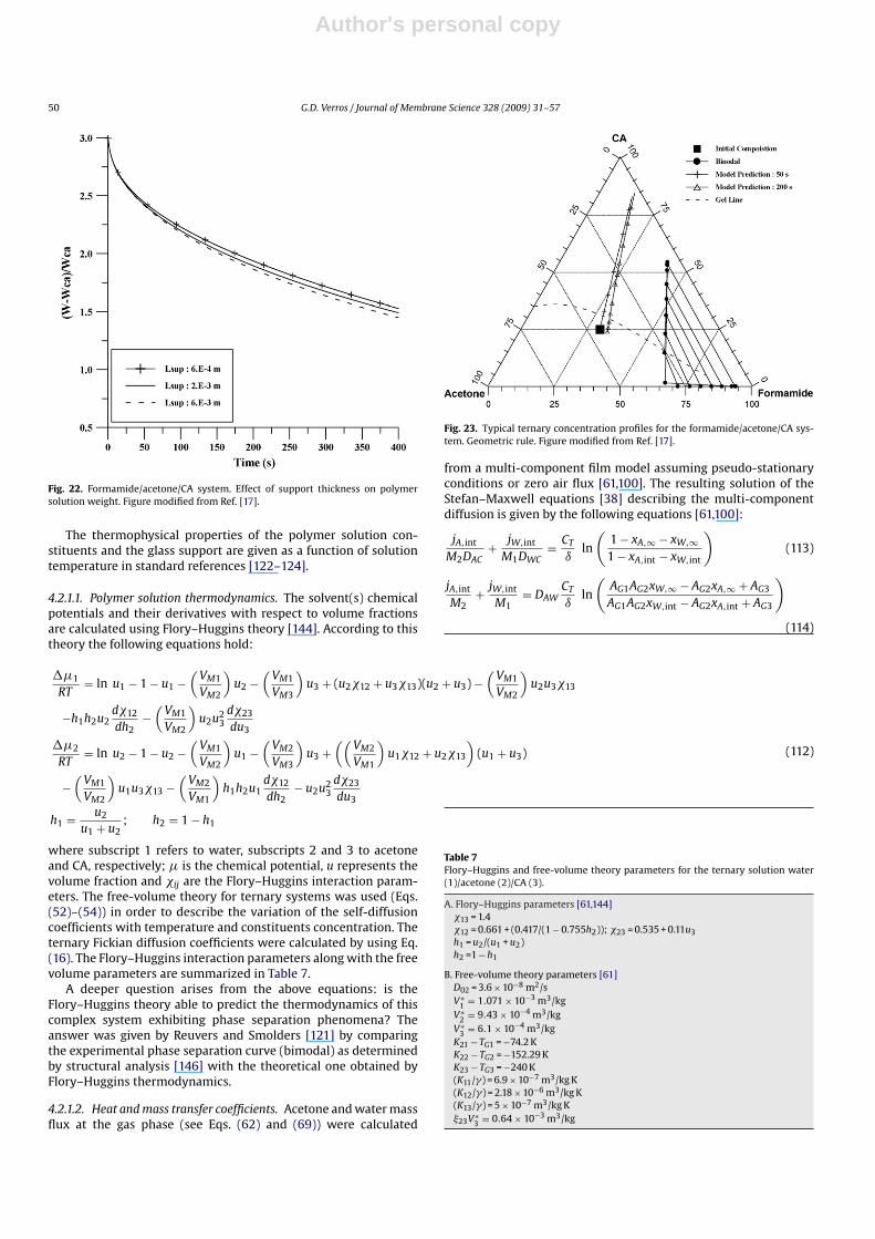
Author's personal copy

50 G.D. Verros / Journal of Membrane Science 328 (2009) 31–57

Fig. 22. Formamide/acetone/CA system. Effect of support thickness on polymersolution weight. Figure modified from Ref. [17].

The thermophysical properties of the polymer solution con-stituents and the glass support are given as a function of solutiontemperature in standard references [122–124].

4.2.1.1. Polymer solution thermodynamics. The solvent(s) chemicalpotentials and their derivatives with respect to volume fractionsare calculated using Flory–Huggins theory [144]. According to thistheory the following equations hold:

��1

RT= ln u1 − 1 − u1 −

(VM1

VM2

)u2 −

(VM1

VM3

)u3 + (u2�12 + u3�13)(u2 + u3) −

(VM1

VM2

)u2u3�13

−h1h2u2d�12

dh2−(

VM1

VM2

)u2u2

3d�23

du3

��2

RT= ln u2 − 1 − u2 −

(VM1

VM2

)u1 −

(VM2

VM3

)u3 +

((VM2

VM1

)u1�12 + u2�13

)(u1 + u3)

−(

VM1

VM2

)u1u3�13 −

(VM2

VM1

)h1h2u1

d�12

dh2− u2u2

3d�23

du3

h1 = u2

u1 + u2; h2 = 1 − h1

(112)

where subscript 1 refers to water, subscripts 2 and 3 to acetoneand CA, respectively; � is the chemical potential, u represents thevolume fraction and �ij are the Flory–Huggins interaction param-eters. The free-volume theory for ternary systems was used (Eqs.(52)–(54)) in order to describe the variation of the self-diffusioncoefficients with temperature and constituents concentration. Theternary Fickian diffusion coefficients were calculated by using Eq.(16). The Flory–Huggins interaction parameters along with the freevolume parameters are summarized in Table 7.

A deeper question arises from the above equations: is theFlory–Huggins theory able to predict the thermodynamics of thiscomplex system exhibiting phase separation phenomena? Theanswer was given by Reuvers and Smolders [121] by comparingthe experimental phase separation curve (bimodal) as determinedby structural analysis [146] with the theoretical one obtained byFlory–Huggins thermodynamics.

4.2.1.2. Heat and mass transfer coefficients. Acetone and water massflux at the gas phase (see Eqs. (62) and (69)) were calculated

Fig. 23. Typical ternary concentration profiles for the formamide/acetone/CA sys-tem. Geometric rule. Figure modified from Ref. [17].

from a multi-component film model assuming pseudo-stationaryconditions or zero air flux [61,100]. The resulting solution of theStefan–Maxwell equations [38] describing the multi-componentdiffusion is given by the following equations [61,100]:

jA,int

M2DAC+ jW,int

M1DWC= CT

ıln

(1 − xA,∞ − xW,∞1 − xA,int − xW,int

)(113)

jA,int

M2+ jW,int

M1= DAW

CT

ıln

(AG1AG2xW,∞ − AG2xA,∞ + AG3

AG1AG2xW,int − AG2xA,int + AG3

)(114)

Table 7Flory–Huggins and free-volume theory parameters for the ternary solution water(1)/acetone (2)/CA (3).

A. Flory–Huggins parameters [61,144]�13 = 1.4�12 = 0.661 + (0.417/(1 − 0.755h2)); �23 = 0.535 + 0.11u3h1 = u2/(u1 + u2)h2 =1 − h1

B. Free-volume theory parameters [61]D02 = 3.6 × 10−8 m2/sV∗

1 = 1.071 × 10−3 m3/kgV∗

2 = 9.43 × 10−4 m3/kgV∗

3 = 6.1 × 10−4 m3/kgK21 − TG1 = −74.2 KK22 − TG2 = −152.29 KK23 − TG3 = −240 K(K11/�) = 6.9 × 10−7 m3/kg K(K12/�) = 2.18 × 10−6 m3/kg K(K13/�) = 5 × 10−7 m3/kg K�23V∗

3 = 0.64 × 10−3 m3/kg

Author's personal copy

G.D. Verros / Journal of Membrane Science 328 (2009) 31–57 51

AG1 =(

(1/DAW ) − (1/DAC )(1/DAW ) − (1/DWC )

); AG2 = (jA,int + jW,int)/jA,int;

AG3 =(

(1/DAC ) − (1/DWC )(1/DAW ) − (1/DWC )

)(115)

DAC, DWC and DAW are the diffusion coefficients of acetone in air,water in air and acetone in water vapor, respectively. CT is the over-all molar concentration and ı is the thickness of the free convectionlayer. The latter was estimated from the binary acetone–air diffu-sion coefficient and the respective mass transfer coefficient kG asfollows [61]:

ı = DACcT MA/(kGP);

kG = 0.54(Gr Sc)0.25(

cT DAC

W

) 1 − xA,int

PxA,intln

(1

1 − xA,int

)(116)

where P denotes the total pressure of the gas phase and Sc is theSchmidt number. The above mass transfer coefficient kG, is calcu-lated from the heat transfer coefficient, h, by invoking the heat andmass transfer analogy and using a correction term for high fluxes,obtained from film theory.

The acetone, xA,int, and the water, xw,int, mole fraction at theinterface, can be written in terms of their activities on the polymersolution side, ˛1 and ˛2 as

xw,int = ˛1Psat1 /P; xA,int = ˛2Psat

2 /P (117)

where Psati

is the pure substance vapor pressure calculated byAntoine’s equation [121]. The activities are related to the respectivechemical potential in the solution by the following equation:

˛i = e��iRT ; i = 1, 2 (118)

where the chemical potentials are calculated from Flory–Hugginstheory. Finally, the emissivity of the ternary solution was equal to0.8 according to the thermographic measurements of Greenberg etal. [129].

4.2.2. Results and discussion: the water/acetone/cellulose acetatesystem

In order to check the idea for the estimation of diffusion coef-ficients Verros and Malamataris [61,100] compared the numericalresults with the experimental work of Shojaie et al. [113,114,129].They used the geometric rule approach and the idea of estimatingresistance (friction) coefficients between solvent molecules frombinary diffusion data.

In particular, Shojaie et al. [113,114] and Greenberg et al. [129]measured the polymer solution weight vs. time, they utilized ther-mographic imaging techniques to measure the polymer solutionsurface temperature and real time reflectometry to detect the onsetof aggregate formation. The on-line turbidity data of Shojaie et al.[113,114] was also taken into account to detect the one-phase regionof the solution by considering their gravimetric and temperaturedata until the point that turbidity of the solution rapidly increaseddue to possible crystalline formation causing further phase sepa-ration. The experimental set-up is identical to the computationaldomain in Fig. 1. The experimental conditions are given in Table 8.

In the model that we have presented in the previous sections, theunknown parameters of the self-diffusion coefficient correlationare the quantities �13 and D01 (see Eqs. (52)–(54)). Verros and Mala-mataris [61,100] estimated these parameters by fitting the modelpredictions of the polymer solution weight vs. time (evaporationrate) with the corresponding data of Shojaie et al. [113,114], usingnon-linear regression analysis. The applied methodology for thecalculation of R12 resistance coefficient from binary diffusion datais given in full detail elsewhere [56,57,113,114].

Table 8Model parameters for the water/acetone/CA system [113,114,129].

Quantity Value Units

Initial temperature, T0 297 ± 0.5 KThickness of the glass support, Lsup 1.2 × 10−3 mCA acetyl Content 39.8%CA molecular weight 40,000 g/mol

Casting surface Calculated from initial conditions

Experiment AInitial acetone weight fraction 0.7Initial water weight fraction 0.2Initial thickness, L0 266 �m

Experiment BInitial acetone weight fraction 0.75Initial water weight fraction 0.1Initial thickness, L0 195 �m

The calculated values for �13, by using the geometric ruleapproach and estimation of R12 resistance coefficient frombinary acetone–water diffusion data, are 0.245 and 0.27, respec-tively. The corresponding values for D01 are 2.5 × 10−9 m2/s and4.6 × 10−9 m2/s, respectively [61,100]. The estimated values forthe water diffusion coefficient at 20 ◦C in the limit of pure CAare 7.25 × 10−12 m2/s and 9.24 × 10−12 m2/s, respectively. The mea-sured diffusion coefficient of water vapor in CA is 1.5 × 10−12 m2/sto 2.3 × 10−12 m2/s [147,148]. It should be noted that the estimatedvalues of the CA–liquid water diffusion coefficient in the limit ofzero acetone concentration are in the same order of magnitudeas the diffusion coefficient of water vapor in cellulose acetate.The observed discrepancy is attributed to the inherent differencesbetween the sorption vapor technique and the experimental set-up[113,114,129].

In the estimation procedure for the values of D01 and �13, bothexperiments of Table 8 were taken into account. The maximumevaporation time in each experiment was determined by the onsetof aggregates-crystalline phase formation [121,146]. Fig. 24 illus-trates the resulting fitting as obtained by Verros and Malamataris[61,100].

Fig. 24. Water/acetone/CA system. Comparison of model predictions [61,100] forpolymer solution weight with experimental data [113,114,129].

Author's personal copy

52 G.D. Verros / Journal of Membrane Science 328 (2009) 31–57

Fig. 25. Water/acetone/CA system. Model predictions [100] for polymer solutionsurface temperature vs. experimental data [113,114,129].

The satisfactory agreement between experimental data andmodel predictions completely justifies the assumptions used. Thepredictive abilities of the model as well as the accuracy of the modelparameters was validated against the variation of the polymer solu-tion surface temperature vs. time as shown in Fig. 25 (modified fromRef. [100]).

Additionally, it was shown in our previous work [61] that theevaporation process is mainly controlled by the diffusion in thepolymer solution, which is the limiting step. Possible errors dueto uncertainty in the estimation of the emissivity are negligible asshown in the previous sections.

The computational method employed enables a deep insightinto the morphology of the resulting membrane, by studying theconcentration profiles of the constituents of the solution. In Fig. 26(modified from Ref. [61]), how the acetone volume fraction changeswith the dimensionless depth of the solution at three differenttime instances is shown. The acetone concentration increases withincreasing length up to a certain point very close to the gas liquidinterface, where a steep decrease is observed.

The corresponding variation of the CA profiles is given in Fig. 27(modified from Ref. [61]). Since the fluxes of acetone and waterare unidirectional from the bottom up to the interface, the exis-tence of local and global extrema in the concentration profilesare surprising at first glance [61]. The concentration profiles ofCA shown in Fig. 27 exhibit steep gradients near the gas liquidinterface of the solution. According to Verros and Malamataris[61] this calculation is in accordance with observations of SEM[113,114,149]. The region of high CA concentration is known to themembranologists as “skin”, which is responsible for the separa-tion properties of asymmetric membranes. The presence of watercauses this phenomenon, because, in the evaporation process ofacetone from binary CA–acetone or formamide/acetone/CA solu-tions, steep profiles have neither been calculated [17,113,114] norobserved [113,114,149]. Moreover, it is shown that skin is formed insitu from the early stages of the evaporation step [61].

In Fig. 28 (modified from Ref. [61]), how the water volume frac-tion varies with the dimensionless depth of the solution at the sametime instances is illustrated. A local minimum and maximum areobserved in the water concentration profiles. Almost identical pro-

Fig. 26. Water/acetone/CA system. Typical acetone concentration profiles, con-ditions as experiment A in Table 8. Estimation of the acetone–water resistancecoefficient from binary data. Figure modified from Ref. [61].

files were obtained by using the geometric rule and the idea ofestimating the resistance coefficient R12 from binary diffusion data.

Regarding the phase separation phenomena our numericalexperiments [61,100] indicate that the system is outside the liq-uid–liquid demixing area and inside the gelation area [100]. There-fore, phase separation occurs after the increase in turbidity due topossible crystallite formation and liquid–solid demixing [100].

In order to explain the profiles shown in Figs. 26–28, a closer lookat the values of the diffusion coefficients should be made. Indeed,Figs. 29–32 depict the variation of the Fickian diffusion coefficients(see Eq. (16)) with constituent concentration.

Fig. 27. Water/acetone/CA system. Typical CA concentration profiles, conditions asexperiment A in Table 8. Estimation of the acetone–water resistance coefficient frombinary diffusion data. Figure modified from Ref. [61].

Author's personal copy

G.D. Verros / Journal of Membrane Science 328 (2009) 31–57 53

Fig. 28. Water/acetone/CA system. Typical water concentration profiles, conditionsas experiment A in Table 8. Estimation of the acetone–water resistance coefficientfrom binary diffusion data. Figure modified from Ref. [61].

Fig. 29. Water (1)/acetone (2)/CA (3) system. Variation of D11 ternary diffusioncoefficient. Geometric rule—temperature 15 ◦C.

Fig. 30. Water (1)/acetone (2)/CA (3) system Variation of D12 ternary diffusion coef-ficient. Geometric rule—temperature 15 ◦C.

Fig. 31. Water (1)/acetone (2)/CA (3) system Variation of D21 ternary diffusion coef-ficient. Geometric rule—temperature 15 ◦C.

An explanation of the profiles obtained in Figs. 26–28 in termsof the diffusion coefficient was given in our previous work [61,100].

An independent test of the diffusion coefficients that could indi-cate potential problems would be of great value [150–152]. Kirkaldyet al. [150] examined the behavior of isothermal, isobaric systemsand showed that Onsager consistency and thermodynamic stabil-ity require that the matrix of diffusion coefficients have real andpositive eigenvalues. The diffusion matrix of a ternary system hasreal and positive eigenvalues, if the following equations hold:

D11 + D22 > 0, D11D22 − D12D21 ≥ 0,

(D11 + D22)2 ≥ 4(D11D22 − D12D21) (119)

These conditions are also satisfied for the diffusion coefficients pre-sented earlier [100].

It should be noted, that the calculated CA concentration profilesjustify the ability of the present model to estimate the diffusioncoefficients near the pure polymer limit, as the polymer concen-tration at the solution–air interface becomes very high [61].

Fig. 32. Water (1)/acetone (2)/CA (3) system. Variation of D22 ternary diffusioncoefficient. Geometric rule—temperature 15 ◦C.

Author's personal copy

54 G.D. Verros / Journal of Membrane Science 328 (2009) 31–57

5. Conclusions

In this work, the solvent evaporation method for the estimationof the Fickian diffusion coefficients in binary and multi-componentsolvent(s)–polymer systems was reviewed. This method combinesthe advantages of both numerical and laboratory experiments. Thenumerical experiment consists: (i) of formulating the mass andenergy conservation equations of the evaporation process alongwith the appropriate boundary and initial conditions, (ii) of solvingthe resulting non-linear system of equations with the finite elementmethod. The laboratory experiment consists of acquiring gravimet-ric data of the polymer solution weight vs. time. The unknownparameters of the self-diffusion coefficient equation, based on free-volume theory, are determined using non-linear regression analy-sis. The described technique was applied to estimate the diffusioncoefficients in the binary systems acetone/cellulose acetate and sol-vent/PVAC. The estimated diffusion coefficients were found in goodagreement with those measured by other methods. Moreover, theternary diffusion coefficients of the water/acetone/cellulose acetatesystem and the resulting asymmetric membrane morphology wereexamined in detail. It is believed that this review could contributeto the further understanding of the behavior of polymer systemsduring the diffusion process.

Acknowledgments

This work has been sponsored by the Archimedes grant ofthe Hellenic Science Foundation. George Verros thanks Ms. KateSomerscales for her help in preparing the manuscript. Finally, theanonymous reviewers of this work are acknowledged for their con-structive comments.

Nomenclature

ac thermal expansion coefficient for the total sum ofthe specific interstitial free volume and specificoccupied volume (K−1)

ai thermal expansion coefficient of the i-th substance(K−1)

AF free-volume theory proportionality constant(mol/m3)

Ai, AGi auxiliary parameters, dimensionlessB auxiliary parameter (kg/(m s))ci molar concentration of the i-th substance (mol/m3)cT total molar concentration (mol/m3)Ci, CTi auxiliary parameter, dimensionlessCp specific heat capacity (J/(kg K))Cp0 scaling factor (J/(kg K))CWLF

12 Williams–Landel–Ferry equation constant, dimen-sionless

CWLF22 Williams–Landel–Ferry equation constant (K)

D0 scaling factor (m2/s)Dij diffusion coefficient (m2/s)DT

ithermal diffusion coefficient (kg/(m s))

DTi auxiliary parameter (m2/s)D∗

iauxiliary parameter (m2/s)

Di self-diffusion coefficient of the i-th substance (m2/s)D0i pro-exponential factor (m2/s)E activation energy (J/gmol)ET auxiliary parameter (J2 m2 s2 mol2/kg2)Eij auxiliary parameter (J m s mol/kg)f GH1 auxiliary free volume parameter, dimensionless

Fi external forces per mole (N/gmol)h heat transfer coefficient (W/(m2 K))�Hi i-th substance latent heat of vaporization (J/kg)ji mass flux of the i-th substance measured relative to

the centre of mass (kg/(m2 s))ji-th mass flux of the i-th substance at the liquid–gas

interface (kg/(m2 s))jVi

mass flux of the i-th substance defined relative tothe volume average velocity (kg/(m2 s))

J∗i

molar flux defined relative to the velocity v of thecentre of mass (mol/(m2 s))

J /=i

, Ji molar flux defined relative to an arbitrary velocity(mol/(m2 s))

k thermal conductivity (W/(m K))kG mass transfer coefficient in the gas phase (kg/m2 Pa)K1i free volume parameter (m3/(kg K))K2i free volume parameter (K)L0 polymer solution initial axial depth (m)Lsup support axial depth (m)Mi molecular weight of the i-th substance (g/mol)P gas pressure (Pa)Ph hydrostatic pressure (Pa)P̃ reduced pressure, dimensionlessP∗

iSanchez–Lacombe equation constant for the i-thsubstance (Pa)

P∗m Sanchez–Lacombe equation parameter for the mix-

ture (Pa)r Sanchez–Lacombe equation parameter, dimension-

lessri Sanchez–Lacombe equation constant for the i-th

substance, dimensionlessR universal gas constant (J/(mol K))R /=

ijfriction coefficient between the i-th and j-th sub-

stance (J m s/mol2)Ri weighted residual, dimensionlesss position of the moving boundary, dimensionlessS rate of entropy production per unit volume

(J/(K m3))t time (s)T temperature (K)TG glass transition temperature (K)T0 initial temperature (K)T̃ reduced temperature, dimensionlessT∗

iSanchez–Lacombe equation constant for the i-thsubstance (K)

T∗m Sanchez–Lacombe equation parameter for the mix-

ture (K)ui volume fraction of i-th substance, dimensionlessui0 initial volume fraction of i-th substance, dimension-

lessv velocity of the centre of mass (m/s)vi local velocity (m/s)v /= arbitrary velocity (m/s)vV volume average velocity (m/s)v∗

iSanchez–Lacombe equation constant for the i-thsubstance (m3/gmol)

v∗m Sanchez–Lacombe equation parameter for the mix-

ture (m3/gmol)V(0) solvent molar volume at 0 K (m3/mol)Vc solvent critical molar volume (m3/mol)V̂ specific volume (m3/kg)

Author's personal copy

G.D. Verros / Journal of Membrane Science 328 (2009) 31–57 55

V̂0 specific occupied volume of a liquid (m3/kg)V̂F specific free volume (m3/kg)VFH average specific hole free volume (m3/kg)V̂FH specific hole free volume (m3/kg)V̂FI specific interstitial free volume (m3/kg)VMi partial molar volume of the i-th substance (m3/mol)V∗

ispecific critical hole free volume of the i-th sub-stance (m3/kg)

V̄i partial specific volume of the i-th substance (m3/kg)V0

i(T) specific volume of the pure i-th substance at tem-

perature T (K) (m3/kg)wi weighting factors whose sum is equal to unity,

dimensionlesswr solvent/polymer mass ratio, dimensionlessW width of the support (m)xi mole fraction, dimensionlessxi,int mole fraction of the i-th substance at the liquid

layer–gas phase interfacexi,∝ mole fraction of the i-th substance at the gas phase

far away from the interfaceXi thermodynamic driving force for diffusion

(J/(gmol m))X ′

itransformed thermodynamic driving forces for dif-fusion (J/(gmol m))

X12 Sanchez–Lacombe equation parameter, dimension-less

z axial coordinate (m)

Greek letters˛ activity, dimensionless� overlap factor, dimensionlessı thickness of the free convection layer (m)ε emissivity of the polymer solution, dimensionlessεij, εm Sanchez–Lacombe equation parameters (J/gmol)� adjustable parameter, dimensionless dimensionless depthp(T) viscosity of pure polymer at temperature T

(kg/(m s))s(T) viscosity of pure solvent at temperature T (kg/(m s))� dimensionless temperature�i chemical potential of the i-th substance (J/mol)� ratio of the critical molar volume of the solvent

jumping unit to the polymer-jumping unit criticalmolar volume, dimensionless

� total mass density (kg/m3)�0 scaling parameter (kg/m3)�i mass density of the i-th substance (kg/m3)�s density of the polymer solution (kg/m3)�̃ reduced density, dimensionless�0

idensity of the i-th pure substance (kg/m3)

�∗i

Sanchez–Lacombe equation constant for the i-thsubstance (kg/m3)

�∗m Sanchez–Lacombe equation parameter for the mix-

ture (kg/m3) Stefan–Boltzman constant (W/m2 K4) dimensionless timeϕi segment fraction, dimensionlessϕi quadratic basis functions, dimensionless� Flory–Huggins coefficient, dimensionless� dissipation function J/(m3 s)ωi weight fraction of the i-th substance, dimensionless

Subscriptint interfaces solutionsup properties and variables of the support

Superscriptf properties of the gas phase

References

[1] S. Loeb, S. Sourirajan, Sea water demineralization by means of an osmoticmembrane, Adv. Chem. Ser. 38 (1962) 117.

[2] R.E. Kesting, Synthetic Polymeric Membranes A Structural Perspective, Wiley,NY, 1985.

[3] I. Pinnau, W.J. Koros, Structure and gas seperation properties of asymmetricpolysulfone membranes made by dry, wet and dry wet phase inversion, J.Appl. Polym. Sci. 43 (1991) 1491.

[4] D.R. Paul, Y.P. Yampolskii (Eds.), Polymeric Gas Separation Membranes, CRCPress, Boca Raton, 1994.

[5] R.A. Cairncross, S. Jeyadef, R.F. Dunham, K. Evans, L.F. Francis, L.E. Scriven, Mod-eling and design of an industrial dryer with convective and radiant heating, J.Appl. Polym. Sci. 58 (1995) 1279.

[6] D. Stoye, W. Freitag (Eds.), Paints, Coatings and Solvents, Wiley-VCH, Wein-heim, 1998.

[7] R.J. Albalak (Ed.), Polymer Devolatilization, Marcel Dekker, NY, 1996.[8] G.D. Verros, T. Latsos, D.S. Achilias, Development of a unified framework for

calculating molecular weight distribution in diffusion controlled free radicalhomopolymerization, Polymer 46 (2005) 539.

[9] S.T. Ju, J.L. Duda, J.S. Vrentas, Influence of temperature on the diffusion ofsolvents in polymers above the glass transition temperature, Ind. Eng. Chem.Prod. Res. Dev. 20 (1981) 330.

[10] J.S. Vrentas, C.M. Vrentas, N. Faridi, Effect of solvent size on solventself-diffusion in polymer–solvent systems, Macromolecules 29 (9) (1996)3272.

[11] C.F. Curtiss, R.B. Bird, Multicomponent diffusion in polymeric liquids, Proc.Natl. Acad. Sci. U.S.A. 93 (1996) 7440.

[12] S. Alsoy, J.L. Duda, Modeling of multicomponent drying of polymer films,AIChE J. 45 (4) (1999) 896.

[13] J.M. Zielinski, B.F. Hanley, Practical friction-based approach to modeling mul-ticomponent diffusion, AIChE J. 45 (1999) 1.

[14] E.B. Nauman, J. Savoca, An engineering approach to an unsolved problem inmulticomponent diffusion, AIChE J. 47 (2001) 1016.

[15] M. Dabral, L.F. Francis, L.E. Scriven, Drying process paths of ternary polymersolution coating, AIChE J. 48 (2002) 25.

[16] P.E. Price Jr., I.H. Romdhane, Multicomponent diffusion theory andits applications to polymer–solvent systems, AIChE J. 49 (2) (2003)309.

[17] G.D. Verros, N.A. Malamataris, Multi-component diffusion in polymer solu-tions, Polymer 46 (2005) 12626.

[18] J.S. Vrentas, J.L. Duda, Diffusion in polymer–solvent systems. I. Re-examination of the free-volume theory, J. Polym. Sci. Part B: Polym. Phys. 15(1977) 403.

[19] J.S. Vrentas, J.L. Duda, Diffusion in polymer–solvent systems. II. A predictivetheory for the dependence of diffusion coefficients on temperature. Concen-tration and molecular weight, J. Polym. Sci. Part B: Polym. Phys. 15 (1977)417.

[20] J.G. Crank, S. Park, Methods of measurement, in: J. Crank, G.S. Park (Eds.),Diffusion in Polymers, Academic Press, 1968, pp. 1–39.

[21] H.J.V. Tyrrell, K.R. Harris, Diffusion in Liquids A Theoretical and ExperimentalStudy, Butterworths, London, 1984.

[22] S.F. Kistler, L.E. Scriven, Coating flows, in: J.R.A. Pearson, S.M. Richardson (Eds.),Computational Analysis of Polymer Processing, Appl. Sci. Publ., London, 1983,pp. 243–299.

[23] P.M. Gresho, R.L. Sani, Incompressible Flow and the Finite Element Method,Wiley, NY, 1998.

[24] C. Truesdell, Mechanical basis of diffusion, J. Chem. Phys. 37 (1962) 2336.[25] A. Fick, Über diffusion, Ann. Phys. 94 (1855) 59.[26] J.C. Slattery, Advanced Transport Phenomena, Cambridge University Press,

Cambridge, 1999.[27] R.B. Bird, W.E. Stewart, E.N. Lightfoot, Transport Phenomena, John Wiley &

Sons, NY, 2002.[28] J.C. Maxwell, Illustrations of the dynamical theory of gases, Philos. Mag. XIX

(1860) 19.[29] J.C. Maxwell, Illustrations of the dynamical theory of gases, Philos. Mag. XX

(1868) 21.[30] J.C. Maxwell, Illustrations of the dynamical theory of gases, Philos. Mag. XX

(1868) 33.[31] J. Stefan, On the equilibrium and movement of gas mixtures. In particular

diffusion, Sitzungsber. Kais. Akad. Wiss. Wien. LXIII (2) (1871) 63.

Author's personal copy

56 G.D. Verros / Journal of Membrane Science 328 (2009) 31–57

[32] J. Stefan, On the dynamical theory of diffusion of gases, Sitzungsber. Kais.Akad. Wiss. Wien. LXV (2) (1872) 323.

[33] C.F. Curtiss, Symmetric gaseous diffusion coefficients, J. Chem. Phys. 49 (19682917).

[34] D.W. Condiff, On symmetric multicomponent diffusion coefficients, J. Chem.Phys. 51 (1969) 4209.

[35] C.F. Curtiss, B.R. Bird, Multicomponent diffusion, Ind. Eng. Chem. Res. 38(1999) 2515.

[36] E.L. Cussler, Multicomponent Diffusion, Elsevier, Amsterdam, 1976.[37] E.L. Cussler, Diffusion Mass Transfer in Fluid Systems, Cambridge Univ. Press,

Cambridge, 1997.[38] R. Taylor, R. Krishna, Multicomponent Mass Transfer, Wiley, New York, 1993.[39] D. Matuszak, M.D. Donohue, Inversion of multicomponent diffusion equa-

tions, Chem. Eng. Sci. 60 (2005) 4359.[40] L. Onsager, R.M. Fuoss, Irreversible processes in electrolytes: diffusion, con-

ductance, and viscous flow in arbitrary mixtures of strong electrolytes, J. Phys.Chem. 36 (1932) 2689.

[41] R.W. Laity, An application of irreversible thermodynamics to the study ofdiffusion, J. Phys. Chem. 63 (1959) 80.

[42] R.J. Bearman, J.G. Kirkwood, The statistical mechanics of transport processes.XI. Equations of transport in multicomponent systems, J. Chem. Phys. 28(1958) 136.

[43] R.J. Bearman, On the molecular basis of some current theories of diffusion, J.Phys. Chem. 65 (1961) 1961.

[44] L. Onsager, Reciprocal relations in irreversible processes I, Phys. Rev. 37 (1931)405.

[45] L. Onsager, Reciprocal relations in irreversible processes II, Phys. Rev. 37 (1931)2265.

[46] H.J. Merk, The macroscopic equations for simultaneous heat and mass transferin isotropic, continuous and closed systems, Appl. Sci. Res. A 8 (1959) 73.

[47] J.S. Vrentas, J.L. Duda, H.C. Ling, Enhancement of impurity removal from poly-mer films, J. Appl. Polym. Sci. 30 (1985) 4499.

[48] J.S. Vrentas, C.M. Vrentas, Drying of solvent-coated polymer films, J. Polym.Sci. Part B: Polym. Phys. 32 (1994) 187.

[49] J. Crank, The Mathematics of Diffusion, Clarendon Press, Oxford, 1975.[50] R.J. Bearman, Statistical mechanical theory of the diffusion coefficients in

binary liquid solutions, J. Chem. Phys. 32 (1960) 1308.[51] J.L. Duda, Y.C. Ni, J.S. Vrentas, An equation relating self-diffusion and mutual

diffusion coefficients in polymer–solvent systems, Macromolecules 12 (1979)459.

[52] J.S. Vrentas, C.M. Vrentas, A new equation relating self-diffusion and mutualdiffusion coefficients in polymer–solvent systems, Macromolecules 26 (1993)6129.

[53] J.S. Vrentas, C.M. Vrentas, Prediction of mutual diffusion coefficients forpolymer–solvent systems, J. Appl. Polym. Sci. 77 (2000) 3195.

[54] P.J. Flory, Principles of Polymer Chemistry, Cornell Univ. Press, Ithaca, NY, 1953.[55] J.S. Vrentas, J.L. Duda, H.C. Ling, Self-diffusion in polymer–solvent–solvent

systems, J. Polym. Sci.: Polym. Phys. 22 (1984) 459.[56] A.J. Reuvers, J.W.A. van den Berg, Formation of membranes by means of

immersion precipitation. Part I. A model to describe mass transfer duringimmersion precipitation, J. Membr. Sci. 34 (1987) 45.

[57] C.S. Tsay, A.J. McHugh, Mass transfer modeling of asymmetric membraneformation by phase inversion, J. Polym. Sci. Part B: Polym. Phys. 28 (1990)1327.

[58] P. Radovanovic, S.W. Thiel, S.T. Hwang, Formation of asymmetric polysul-fone membranes by immersion precipitation. Part I. Modeling mass transportduring gelation, J. Membr. Sci. 65 (1992) 2.

[59] S.S. Shojaie, W.B. Krantz, A.R. Greenberg, Dense polymer film and membraneformation via the dry-cast process. Part I. Model development, J. Membr. Sci.94 (1994) 255.

[60] L.P. Cheng, Y.S. Soh, A.H. Dwan, C.C. Gryte, An improved model formass transfer during the formation of polymeric membranes by theimmersion–precipitation process, J. Polym. Sci. Part B: Polym. Phys. 32 (1994)1413.

[61] G.D. Verros, N.A. Malamataris, Computer aided estimation of diffusion coef-ficients in polymer/non-solvent systems, Macromol. Theory Simul. 10 (2001)737.

[62] J.O. Hirschfelder, C.F. Curtiss, R.B. Bird, Molecular Theory of Gases and Liquids,Wiley, New York, 1964.

[63] S.R. de Groot, P. Mazur, Non-Equilibrium Thermodynamics, Dover Publica-tions, New York, 1984.

[64] G.D.C. Kuiken, Thermodynamics of Irreversible Processes-Applications to Dif-fusion and Rheology, John Wiley & Sons, New York, 1994.

[65] Y.A. Demirel, S.I. Sandler, Nonequilibrium thermodynamics in engineeringand science, J. Phys. Chem. B 108 (1) (2004) 31.

[66] P.J.A.M. Kerkhof, M.A.M. Geboers, Toward a unified theory of isotropic molec-ular transport phenomena, AIChE J. 51 (1) (2005) 79.

[67] A. Schmitt, J.B. Craig, Frictional coefficient formalism and mechanical equilib-rium in membranes, J. Phys. Chem. 81 (13) (1977) 1338.

[68] L. Onsager, Theories and problems of liquid diffusion, Ann. N. Y. Acad. Sci. 46(1945) 241.

[69] D.G. Miller, Application of irreversible thermodynamics to electrolyte solu-tions. I. Determination of ionic transport coefficients lij for isothermal vectortransport processes in binary electrolyte systems, J. Phys. Chem. 70 (8) (1966)2639.

[70] H.B.G. Casimir, On Onsager’s principle of microscopic reversibility, Rev. Mod.Phys. 17 (2-3) (1945) 343.

[71] E.P. Wigner, Derivations of Onsager’s reciprocal conditions, J. Chem. Phys. 22(54) (1954 1912).

[72] D.G. Miller, Thermodynamics of irreversible processes: the experimental ver-ification of the Onsager reciprocal relations, Chem. Rev. 60 (1) (1960) 16.

[73] D.G. Miller, Ternary isothermal diffusion and the validity of the Onsager reci-procity relations, J. Phys. Chem. 63 (8) (1959) 570.

[74] D.P. Kondepudi, I. Prigogine, Thermodynamics nonequilibrium, in: G.L. Trigg(Ed.), Encyclopedia of Applied Physics, Wiley-VCH, 2003.

[75] B.D. Coleman, C. Truesdell, On the reciprocal relations of Onsager, J. Chem.Phys. 33 (1) (1960) 28.

[76] C.A. Truesdell, Rational Thermodynamics, Springer–Verlag, New York, 1984.[77] G.D. Verros, On the validity of the Onsager reciprocal relations in multi-

component diffusion, Phys. Lett. A 365 (2007) 34.[78] J.W. Lorimer, Phenomenological coefficients and frames of reference for trans-

port processes in liquids and membranes. Part I. Resistance coefficients.Friction coefficients and generalized diffusivities in isothermal systems, J.Chem. Soc., Faraday Trans. 2 (74) (1978) 75.

[79] J.W. Lorimer, Phenomenological coefficients and frames of reference for trans-port processes in liquids and membranes. Part II. Resistance coefficients innon-isothermal systems, J. Chem. Soc., Faraday Trans. 2 (74) (1978) 84.

[80] G.D. Verros, On the validity of Onsager reciprocal relations for simulta-neous heat transfer and multi-component diffusion, Physica A 385 (2007)487.

[81] J.S. Vrentas, C.M. Vrentas, Restrictions on friction coefficients for binary andternary diffusion, Ind. Eng. Chem. Res. 46 (10) (2007) 3422.

[82] J.M. Zielinski, A friction factor analysis of the coupling between poly-mer/solvent self- and mutual-diffusion: polystyrene/toluene, J. Polym. Sci.Part B: Polym. Phys. 34 (1996) 2759.

[83] M.H. Cohen, D. Turnbull, Molecular transport in liquids and glasses, J. Chem.Phys. 31 (1959) 1164.

[84] H. Fujita, Diffusion in polymer-dilluent systems, Fortsch. Hochpolym. Forsch.3 (1961) 1.

[85] C.W. Paul, A model for predicting solvent self-diffusion coefficients in nonglassy polymer/solvent solutions, J. Polym. Sci. Polym. Phys. Ed. 21 (1983)425.

[86] J.S. Vrentas, J.L. Duda, H.C. Ling, A.C. Hou, Free-volume theories for self-diffusion in polymer–solvent systems. II. Predictive capabilities, J. Polym. Sci.Polym. Phys. Ed. 23 (1985) 289.

[87] J.S. Vrentas, C.M. Vrentas, Evaluation of free-volume theories for solvent self-diffusion in polymer–solvent systems, J. Polym. Sci. Polym. Phys. Ed. 31 (1993)69.

[88] J.S. Vrentas, C.M. Vrentas, Evaluation of the free-volume theory of diffusion,J. Polym. Sci. Polym. Phys. Ed. 41 (2003) 501.

[89] R.N. Haward, Occupied volume of liquids and polymers, J. Macromol. Sci. Rev.Macromol. Chem. C4 (1970) 191.

[90] J.D. Ferry, Dependence of Viscoelastic Behavior on Temperature and Pressurein Viscoelastic Properties of Polymers, 3rd ed., Wiley, New York, 1980, pp.264–320.

[91] A.K. Doolittle, Studies in Newtonian flow. II. The dependence of the viscosityof liquids on free-space, J. Appl. Phys. 22 (1951) 1471.

[92] F.A.L. Dullien, Predictive equations for self-diffusion in liquids: a differentapproach, AIChE J. 18 (1972) 62.

[93] J.M. Zielinski, J.L. Duda, Predicting polymer/solvent diffusion coefficientsusing free volume theory, AIChE J. 38 (1992) 405.

[94] S. Hong, Prediction of polymer/solvent solution behavior using free-volumetheory, Ind. Eng. Chem. Res. 34 (1995) 2536.

[95] B.G. Wang, H.-L. Lv, J.C. Yang, Estimation of solvent diffusion coefficient inamorphous polymers using the Sanchez–Lacombe equation-of-state, Chem.Eng. Sci. 62 (2006) 775.

[96] M. Ataka, K. Sasaki, Gravimetric analysis of membrane casting. I. Celluloseacetate–acetone binary casting solutions, J. Membr. Sci. 11 (1982) 11.

[97] P.E. Price Jr., S. Wang, I.H. Romdhane, Extracting effective diffusion parametersfrom drying experiments, AIChE J. 43 (1997) 1925.

[98] G.D. Verros, N.A. Malamataris, Estimation of diffusion coefficients inacetone–cellulose acetate solutions, Ind. Eng. Chem. Res. 38 (1999) 3572.

[99] G.D. Verros, S. Papachristou, J. Prinos, N.A. Malamataris, Computer aided esti-mation of the methyl acetate, acetone and chloroform diffusion coefficientsin polyvinyl acetate, Chem. Eng. Commun. 190 (2003) 334.

[100] G.D. Verros, N.A. Malamataris, Estimation of diffusion coefficients in polymersolutions, in: G. Maroulis, T.E. Simos (Eds.), Lecture Series on Computer andComputational Sciences. In the Frontiers of Computational Science, vol. 3, BrillAcademic Publishers, Leiden, The Netherlands, 2005, pp. 360–383.

[101] F. Doumenc, B. Guerrier, Estimating polymer–solvent diffusion coefficient byoptimization procedure, AIChE J. 47 (2001) 984.

[102] J.S. Vrentas, J.L. Duda, Diffusion in polymer–solvent systems. III. Constructionof Deborah number diagrams, J. Polym. Sci. Part B: Polym. Phys. 15 (1977) 441.

[103] B. Guerrier, C. Bouchard, C. Allain, C. Benard, Drying kinetics of polymer films,AIChE J. 44 (4) (1998) 791.

[104] W.D. Murray, F. Landis, Numerical and machine solutions of transient heat-conduction problems involving melting or freezing. Part I. Method of analysisand sample solutions, Trans. ASME, J. Heat Trans. 81 (1959) 106.

[105] P. Murray, G.F. Carey, Finite element analysis of diffusion with reaction at amoving boundary, J. Comp. Phys. 74 (1988) 44.

Author's personal copy

G.D. Verros / Journal of Membrane Science 328 (2009) 31–57 57

[106] P. Hood, Frontal solution program for unsymmetric matrices, Int. J. Num. Meth.Eng. 10 (1976) 379;P. Hood, Correction, Int. J. Num. Meth. Eng. 11 (1977) 1055.

[107] J. Crank, Free and Moving Boundary Problems, Clarendon Press, Oxford, 1988.[108] B.A. Finlayson, Numerical Methods for Problems with Moving Fronts, Ravenna

Park Publishing Inc., Seatle, 1992.[109] J.E. Anderson, R. Ullman, Mathematical analysis of factors influencing the skin

thickness of asymmetric reverse osmosis membranes, J. Appl. Phys. 44 (1973)4303.

[110] W.B. Krantz, R.J. Ray, R.L. Sani, K.J. Gleason, Theoretical study of the transportprocesses occurring during the evaporation step in asymmetric membranecasting, J. Membr. Sci. 29 (1986) 11.

[111] S.B. Tantekin-Ersolmaz, The Evaporation Step in Asymmetric Membrane For-mation: Modeling, Gravimetric/Inframetric, and Morphology Studies, Ph.D.Dissertation, University of Colorado, Boulder, CO, 1990.

[112] C.S. Tsay, A.J. McHugh, Mass transfer dynamics of the evaporation step inmembrane formation by phase inversion, J. Membr. Sci. 64 (1991) 81.

[113] S.S. Shojaie, Polymeric Dense Films and Membranes via the Dry-Cast PhaseInversion Process. Modeling, Casting and Morphological Studies, Ph.D. Thesis,Boulder, CO, 1992.

[114] S.S. Shojaie, W.B. Krantz, A.R. Greenberg, Dense polymer film and membraneformation via the dry-cast process. Part II. Model validation and morpholog-ical studies, J. Membr. Sci. 94 (1994) 281.

[115] H. Matsuyama, M. Teramoto, T. Uesaka, Membrane formation and structuredevelopment by dry-cast process, J. Membr. Sci. 135 (1997) 271.

[116] G.D. Verros, N.A. Malamataris, Finite element analysis of polymeric membraneand coating formation by solvent evaporation, Comput. Mech. 27 (2001) 332.

[117] S.A.B. Alsoy-Altinkaya, Ozbas modeling of asymmetric membrane formationby dry-casting method, J. Membr. Sci. 230 (2004) 71.

[118] H. Lee, S.R. Chaudhuri, W.B. Krantz, S.T. Hwang, A model for evaporativecasting of polymeric membranes incorporating convection due to densitychanges, J. Membr. Sci. 284 (1) (2006) 161.

[119] G.S. Park, Radioactive studies of diffusion in polymer systems. Part 3. Sorptionand self-diffusion in the acetone + cellulose acetate system, Trans. Faraday Soc.57 (1961) 2314.

[120] M.P. Sanopoulou, P. Roussis, J.H. Petropoulos, A detailed study of the viscoelas-tic nature of vapor sorption and transport in a cellulosic polymer. I. Origin andphysical implications of deviations from Fickian sorption kinetics, J. Polym. Sci.Part B: Polym. Phys. 33 (1995) 993.

[121] A.J. Reuvers, C.A. Smolders, Formation of membranes by means of immersionprecipitation. Part II. The mechanism of formation of membranes preparedfrom the system cellulose acetate–acetone–water, J. Membr. Sci. 34 (1987) 67.

[122] J.A. Dean, Lange’s Handbook of Chemistry, 11th ed., McGraw-Hill, New York,1973.

[123] R.H. Perry, D. Green, Perry’s Chemical Engineers’ Handbook, 6th ed., McGraw-Hill, New York, 1984.

[124] Verein Deutscher Ingenieure, VDI-Warmeatlas, VDI-Verlag GmbH, Dusseldorf,1974.

[125] R. Jeffries, The thermodynamic properties of mixtures of secondary celluloseacetate and its solvents, Trans. Faraday Soc. 53 (1957) 592.

[126] F. Altena, Phase Separation Phenomena in Cellulose Acetate Solutions inRelation to Asymmetric Membrane Formation, Ph.D. Dissertation, TwenteUniversity of Technology, Enschede, Netherlands, 1982.

[127] C.R. Wilke, A viscosity equation for gas mixtures, J. Chem. Phys. 18 (1950)517.

[128] E.N. Fuller, P.D. Schettler, J.C. Giddings, A new method for prediction of binarygas-phase diffusion coefficients, Ind. Eng. Chem. 58 (5) (1966) 18.

[129] A.R. Greenberg, S.S. Shojaie, W.B. Krantz, S.B. Tantekin-Ersolmaz, Use ofinfrared thermography for temperature measurement during evaporativecasting of thin polymeric films, J. Membr. Sci. 107 (1995) 249.

[130] R.J. Kokes, vA. Long, J.L. Hoard, Diffusion of acetone into polyvinyl acetateabove and below the second-order transition, J. Chem. Phys. 20 (1952) 1711.

[131] S.T. Ju, H.T. Liu, J.L. Duda, J.S. Vrentas, Solvent diffusion in amorphous polymers,J. Appl. Polym. Sci. 26 (1981) 3735.

[132] D. Arnould, J.L. Laurence, Size effects on solvent diffusion in polymers, Ind.Eng. Chem. Res. 31 (1992) 218.

[133] I.C. Sanchez, R.H. Lacombe, An elementary molecular theory of classical fluids.Pure fluids, J. Phys. Chem. 80 (1976) 2352.

[134] I.C. Sanchez, R.H. Lacombe, Statistical thermodynamics of fluid mixtures, J.Phys. Chem. 80 (1976) 2568.

[135] I.C. Sanchez, C.G. Panayiotou, Equation of state thermodynamics of polymerand related solutions, in: S.I. Sandler (Ed.), Models for Thermodynamic andPhase Equilibrium Calculations, Dekker, New York, 1994.

[136] L. Luengo, R.G. Rabio, I.C. Sanchez, C.G. Panayiotou, The System poly(4-hydroxystyrene)/poly(vinyl acetate)/acetone: an experimental and theoret-ical study, Makromol. Chem. Phys. 195 (1994) 1043.

[137] C.G.I.C. Panayiotou, Sanchez hydrogen bonding in fluids: an equation-of-stateapproach, J. Phys. Chem. 95 (1991) 10090.

[138] S. Manjikian, Desalination from organic casing solutions, Ind. Eng. Chem. Prod.Res. Dev. 6 (1967) 23.

[139] B. Kunst, S. Sourirajan, Evaporation rate and equilibrium phase separation datain relation to casting conditions and performance of porous cellulose acetatereverse osmosis membranes, J. Appl. Polym. Sci. 14 (1970) 1983.

[140] H. Ohya, S. Sourirajan, Determination of concentration changes on membranesurface as function of time during evaporation of reverse-osmosis film castingsolutions, J. Appl. Polym. Sci. 15 (1971) 705.

[141] R. Pilon, B. Kunst, S. Sourirajan, Studies on the development of improvedreverse osmosis membranes from cellulose acetate–acetone–formamidecasting solutions, J. Appl. Polym. Sci. 15 (1971) 1317.

[142] M.A. Frommer, D. Lancet, The mechanism of membrane formation: membranestructures and their relation to preparation conditions, in: H.K. Lonsdale, H.E.Podal (Eds.), Reverse Osmosis Membrane Research, Plenum Press, New York,1972, pp. 85–110.

[143] S. Alsoy Altinkaya, H. Yenal, B. Ozbas, Membrane formation by dry-cast processmodel validation through morphological studies, J. Membr. Sci. 249 (2005)163.

[144] L. Yilmaz, A.J. McHugh, Analysis of nonsolvent–solvent–polymer phase dia-grams and their relevance to membrane formation modeling, J. Appl. Polym.Sci. 31 (1986) 997.

[145] P.M. Fahey, H.E. Grethlein, Improved cellulose acetate membranes for reverseosmosis, Desalination 9 (1971) 297.

[146] A.J. Reuvers, F.W. Altena, C.A. Smolders, Demixing and gelation behavior ofternary cellulose acetate solutions, J. Polym. Sci. Part B: Polym. Phys. 24 (1986)793.

[147] P.P. Roussis, Diffusion of water vapor in cellulose acetate. 1. Differential tran-sient sorption kinetics and equilibria, Polymer 22 (1981) 768.

[148] P.P. Roussis, Diffusion of water vapor in cellulose acetate. 2. Permeation andintegral sorption kinetics, Polymer 22 (1981 1058).

[149] R.L. Riley, J.O. Gardner, V. Merten, Cellulose acetate membranes: electronmicroscopy of structures, Science 143 (1964) 801.

[150] J.S. Kirkaldy, D. Weichert, Zia-Ul-Haq, Diffusion in multicomponent metal-lic systems. VI. Some thermodynamic properties of the D matrix and thecorresponding solutions of the diffusion equations, Can. J. Phys. 41 (1963)2166.

[151] D.G. Miller, V. Vitagliano, R. Sartorio, Some comments on multicomponentdiffusion: negative main term diffusion coefficients, second law constraints,solvent choices, and reference frame transformations, J. Phys. Chem. 90 (1986)1509.

[152] J.S. Vrentas, C.M. Vrentas, Theoretical aspects of ternary diffusion, Ind. Eng.Chem. Res. 44 (2005) 1112.