Shock Waves in Nonequilibrium Gases and Plasmas - DTIC

AFIT/DS/ENP/97D-08

Shock Waves in Nonequilibrium Gases and Plasmas

DISSERTATION

Presented to the Faculty of the School of Engineering

of the Air Force Institute of Technology

Air University

In Partial Fulfillment of the

Requirements for the Degree of

Doctor of Philosophy

WilliamM. Hilhuii. B.S.. M.S.

Major

19971121 091 October 1!M)7

{DTIC QUALITY INSPECTED €

Approved for public release; distribution unlimited

AFIT/DS/ENP/97D-08


William M. Hilbun, B.S., M.S.

Major

Approved:

^3^P.

Q^

Dr. David E. Weeks

J2.

Dr. William F. Bailey, Chairman

/; A A*,*^ MASf? Dr. Philip S. Beran

Dr. Richard F. Deckro

JW If/ %MsZ> 2 -> &7- ?7 Dr. Dennis W. Quinn

Pc/!&>?>~ zz <&/■=? 7

^^C-i//i/^--—-i— Robert A. Calico, JR.

Dean

Acknowledgements

Throughout the course of this research, a number of individuals have been a

great help to me, without whom this dissertation could not have been written. I

would like to express my thanks to Dr. Alan Garscadden and Dr. Joseph Shang,

both of Wright Laboratory, for their continual encouragement of this work. Dr.

Biswa Ganguly (WL/PO) and Dr. Peter Bletzinger (Mobium Enterprises. Inc.) were

extremely generous to me, providing both access to their plasma/shock data and

details on their experimental apparatus. I would like to thank Dr. Charlie DeJoseph

(WL/PO) for providing the basic vibrational kinetics code used in this work. Mr.

Lee Bain (WL/PO) provided funding for travel and Lt Brandon Wood (WL/PO)

was extremely helpful in providing information on issues relating to various aspects

of the research. I would also like to express my gratitude to Mr. Eswar Josyula

(WL/FIMC) for his assistance and patience in the early stages of the research,

particularly with regard to the computational fluid dynamic aspects of the problem.

I wish I knew as much about CFD as Eswar has forgotten. I also wish to express my

thanks to my fellow classmates Major Jim Shoemaker and Captain Eric Bennett,

for acting as a sounding board and a reality check throughout this research, as well

as providing many LaTex tricks along the way. The Major Shared Resource Center

(MSRC) at Wright-Patterson AFB, OH, provided the computer time required for

the calculations in this research and are a tremendous asset to the Air Force with

their computer hardware and technical personnel. I would also like to thank my

adviser. Dr. W.F. Bailey (AFIT/ENP) for his encouragement, support, suggestions

and insight throughout my graduate studies at AFIT. He always came up with good

ideas when I needed them most. Finally. I must express my deep appreciation to

my wife and children for their endless support and encouragement. Without them,

none of this would have been possible.

William M. Hilbun

in

Table of Contents

Page

Acknowledgements iii

List of Figures ix

Abstract xvi

I. Introduction 1

1.1 Motivation 1

1.2 Shocks in a Neutral Gas 3

1.2.1 How Do Shocks Develop? 4

1.2.2 Typical Scale Lengths 5

1.3 Shocks in a Weakly Ionized Nonequilibrium Plasma .... 6

1.3.1 What's New? 6

1.3.2 Typical Scale Lengths 7

1.4 Experimental Anomalies of Shocks in Weakly Ionized Plasma 8

1.5 Possible Applications of Plasma-Aerodynamics 15

1.6 Research Objectives 17

1.7 Previous Work IS

1.7.1 Charge Particle/Neutral Particle Interactions . . 18

1.7.2 Vibrational Energy Relaxation . 22

1.7.3 Thermal Inhomogeneities 24

1.8 Research Approach 25

II. Background Theory 30

2.1 Introduction 30

2.2 Shock Analysis Approaches 30

iv

2.1 Kinetic Approach 31

2.2.2 Fluid Approach 31

2.3 Plasma Effects 33

2.3.1 Small-Amplitude Wave Propagation in Weakly Ion-

ized Plasma 33

2.3.2 Shock Propagation in Weakly Ionized Plasma . . 34

2.4 Post-Shock Energy Addition: Vibrational Relaxation ... 45

2.4.1 Shocks and Hugoniot Shock Adiabatics 45

2.4.2 Nonequilibrium Vibrational Relaxation Time . . . 55

2.5 Thermal Inhomogeneities 64

III. Plasma Effects 68

3.1 Introduction 68

3.2 Steady-State Analysis 69

3.2.1 Model Equations 69

3.2.2 Steady-State Results 71

3.3 Time-Dependent Analysis 79

3.3.1 Model Equations 79

3.3.2 Code Validation 83

3.3.3 Time-Dependent Results . 89

3.4 Conclusion 95

IV. Vibrational Energy Relaxation Effects 100

4.1 Introduction 100

4.2 Influence of Energy Addition on Shock Speed 101

4.2.1 Model Equations ■ . . 101

4.2.2 Code Validation 103

4.2.3 Numerical Results 107

2.4 Analytic Determination of Shock Speed Ill

4.3 Analysis of Vibrational Kinetics 118

4.3.1 How Much Energy Can Be Released? 118

4.3.2 How Fast Can the Energy Be Released? 122

4.4 Conclusion 124

V. Thermal Effects 127

5.1 Introduction 127

5.2 Model Equations 129

5.3 Code Validation 132

5.3.1 Riemann Problem 132

5.3.2 Spark-Initiated Shock 137

5.4 Step Temperature Rise 142



5.5 Radial Temperature Profile 154



5.6 Comparison to Experiment . 167



5.7 Conclusion 187

VI. Conclusions/Recommendations 189

6.1 Computational Codes 189

6.2 Charged Particle/Neutral Particle Interactions 191

6.3 Post-Shock Energy Release 192

6.4 Thermal Inhomogeneities 194

6.5 Recommendations • • 196

VI

Page

Appendix A. List of Symbols 198

Appendix B. Two-Dimensional Fluid Dynamics Code Description ... 201

B.l Introduction 201

B.2 Nondimensionalization of Equations 201

B.3 Model Equations (nondimensional) 202

B.4 Strang-Splitting Operators 205

B.4.1 x Sweep Operator 207

B.4.2 y Sweep Operator 209

B.4.3 Source Operator 213

B.5 Initial Conditions 216

B.6 Boundary Conditions 217

B.7 Determination of Time Step 219

B.8 Code Flowchart 220

B.9 Determination of Shock Velocity 222

Appendix C. Two-Fluid Plasma Code Description 224

Appendix D. Self-Consistent Model of Gas Heating in a Glow Discharge 228

D.l Problem Statement 228

D.2 Source Term 230

D.3 Boundary Conditions 232

D.4 Solution Method 232

D.5 Input Parameters 234

D.6 Test Cases and Typical Results 238

Appendix E. Optical Diagnostics in Shock Tubes: A Short Tutorial . . 241

E.l Optical Interferometry 242

E.2 Photo-Acoustic Deflection Spectroscopy 246

Vll

Bibliography

Page

250

Vita 258

vm

List of Figures Figure Page

. 1. Typical variation in gas temperature with distance in a shock. ... 3

2. Temporal evolution of the pressure in a large amplitude wave leading

to the formation of a shock. . 4

3. Typical temperature relaxation processes in a shock 5

4. Electric double layer resulting from diffusion of electrons and ions at

the shock front 7

5. Shock velocity measured in N2 in the absence of a plasma and in a

weakly ionized plasma 9

6. Variation in pressure with time for a shock in air and in plasma. . . 10

7. Variation of the density in a shock wave in air in the presence of a

plasma and in the absence of a plasma 11

8. Variation of the pressure jump at the shock front in air and in a weakly-

ionized plasma in air 12

9. Experimentally determined variation in the aerodynamic drag coeffi-

cient (CD) with velocity for a sphere in unionized air and in weakly

ionized air 13

10. Shock standoff distance measured in weakly ionized plasma and in

unionized gas 14

11. Proposed modification to an existing F-15 aircraft to flight-test plasma-

aerodynamic effects 16

12. AJAX hypersonic vehicle concept 16

13. Research Approach 26

14. Regimes of applicability for the kinetic and fluid equations 30

15. Velocity profiles of ions and neutrals in a weakly ionized plasma . . 41

16. Density profiles of ions and neutrals in a weakly ionized plasma ... 42

17. Electric field profile in a weakly ionized plasma 43

18. Shock adiabatic for a gas with 7=7/5 47

IX

Figure Page

19. Shock adiabatic for a gas (7 = 7/5) and a mass flux line for a shock. 48

20. Comparison of Tvib given by Equation 34 {Tvtbi) with Tvih given by

Equation 35 (TVM) • 49

21. Shock adiabatics for a gas initially in equilibrium 50

22. Temperature distribution for a gas initially in equilibrium 51

23. Shock adiabatics for a gas initially in nonequilibrium 52

24. Temperature distribution for a gas initially in nonequilibrium .... 53

25. Shock adiabatics for a gas initially in nonequilibrium along with three

shocks of varying velocity 54

26. Dependence of the rates Pv,v-i and Q°vd

v_i on the vibrational quantum

number for N2 5"

27. Distribution of N2 molecules in vibrational states under typical nonequi-

librium conditions 58

28. Effective relaxation times in <V2 hi nonequilibrium conditions at various

vibrational temperatures 60

29. Shock adiabatics corresponding to nonequilibrium vibrational relax-

ation in N-2 61

30. Variation in shock velocity ratio (V2/l 1) and Mach number ratio (M2/Mi)

with T2/Ti for a shock incident on an infinite planar thermal interface. 65

31. Variation in pressure ratio at the shock front (P2/P1) with T2/7\ for

a shock incident on an infinite planar thermal interface . 66

32. Velocity of charged component precursor from steady-state analysis. 71

33. Density of charged component precursor from steady-state analysis. 73

34. Electric field at shock front from steady-state analysis • ■ • • "4

35. Contributions of collision and pressure gradient terms to the electric

field at shock front from steady-state analysis 75

36. Net charge density in the shock front region for a Mach 2 shock in

Argon 76

37. Numerically determined peak electric field, potential drop and shock

precursor width compared with analytic estimates 77

x

Figure Page

38. Initial conditions in a typical shock tube 84

39. Analytic and numeric solutions to the Riemann problem in Argon with

neutral-charged particle coupling turned off and Te = 0Ä' : 85

40. Analytically and numerically determined neutral and ion shock speeds

in Argon. • ■ 86

41. Variation of the ion-acoustic velocity with electron temperature for a

small-amplitude wave in Argon • • • 88

42. Velocity of charged component precursor from time-dependent analysis. 90

43. Density of charged component precursor from time-dependent analysis. 91

44. Electric field at shock front from time-dependent analysis 92

45. Variation in the total density with distance in the shock front region

for various degrees of fractional ionization 93

46. Variation in the neutral shock velocity with fractional ionization. . . 94

47. General experimental arrangement in which a shock interacts with a

gas which has been vibrationally excited by the plasma 101

48. Exact and numerical solution of Euler's equations for a gas with a

finite vibrational relaxation time 104

49. Gas temperature and vibrational temperature in the shock front region

for a shock propagating through gas in an equilibrium state 105

50. Numerically and analytically determined shock velocity for the Rie-

mann problem in which the shock propagates through a gas in initial

equilibrium with a finite vibrational relaxation time 106

51. Shock tube used to model the nonequilibrium vibrational relaxation

effects 107

52. Numerical solution of Euler's equations for a gas with a finite vibra-

tional relaxation time 109

53. Gas temperature and vibrational temperature in the shock front region

for a shock propagating through gas in a nonequilibrium state. ... 110

54. Numerically and analytically determined shock velocity for the Rie-

mann problem in which the shock propagates through a gas initially

in a nonequilibrium state • • • HI

XI

Figure Page

55. Variation of the steady-state shock velocity in the nonequilibrium re-

gion with the shock velocity entering the nonequilibrium region. . . 115

56. Nonequilibrium and equilibrium vibrational distribution functions in

A^ 119

57. Maximum amount of vibrational energy (estimated) available for re-

lease into the post-shock region 121

58. Amount of vibrational energy added to the flow for a Mach 3 shock in

N2....\ 123

59. Typical experimental arrangement in which a shock propagates into a

plasma-heated gas 128

60. Analytic and numerical solution to the Riemann problem 133

61. Density and pressure from the two-dimensional numerical solution to

the Riemann problem 135

62. Analytically and numerically determined shock speed along the cen-

terline 136

63. Spark-initiated shock density profile: experiment vs simulation. . . . 138

64. Variation of shock front position with time and resulting shock front

velocity for a spark-initiated shock 139

65. Pressure contours resulting from the propagation of a small-amplitude

wave originating from the center of the domain 141

66. Pressure distribution for a Riemann shock propagating into gas with

a step rise in temperature 143

67. Density distribution for a Riemann shock propagating into gas with a

step rise in temperature 143

68. Variation in the shock velocity as a Riemann shock propagates through

gas with a step rise in temperature 145

69. Variation in pressure ratio at the shock front (P2/P1) as a Riemann

shock propagates through gas with a step rise in temperature. . . . 146

70. Pressure distribution for a Riemann shock propagating into gas with

a step decrease in temperature 148

xn

Figure Page

71. Density distribution for a Riemann shock propagating into gas with a

step decrease in temperature , . . . 148

72. Variation in the shock velocity as a Riemann shock propagates through

gas with a step decrease in temperature 149

73. Variation in pressure ratio at the shock front (P2/Pi) as a Riemann

shock propagates through gas with a step decrease in temperature. . 149

74. Pressure distribution for a spark-initiated shock propagating into gas

with a step rise in temperature. 152

75. Density distribution for a spark-shock propagating into gas with a step

rise in temperature 152

76. Variation in shock speed as a spark-initiated shock propagates through

gas at 300A' and through a gas with a step increase in temperature. 153

77. Variation in the centerline shock velocity as a Riemann shock propa-

gates into a region with a radial thermal inhomogeneity 155

78. Density profiles near the shock front for a Riemann shock propagating

into a region with a radial thermal inhomogeneity 156

79. Two-dimensional distribution of density and pressure in a Riemann

shock propagating into a region with a radial thermal inhomogeneity. 158

80. Pressure contours near the shock front for a Riemann shock propagat-

ing into a region with a radial thermal inhomogeneity with transverse

coupling 161

81. Pressure contours near the shock front for a Riemann shock prop-

agating into a region with a radial thermal inhomogeneity without

transverse coupling 161

82. Variation in shock speed as a spark-initiated shock propagates through

gas with a radial thermal inhomogeneity 162

83. Density profiles as a spark-initiated shock propagates through gas with

a radial thermal inhomogeneity 163

84. Two-dimensional distribution of density and pressure in a spark-initiated

shock propagating into a region with a radial thermal inhomogeneity. 165

Xlll

öe Figure Pag

85. Two-dimensional distribution of density and pressure in a spark-initiated

shock propagating into a gas at 300A 166

86. Radial distribution of gas temperature in a discharge in air (measured) 168

87. Variation in the shock velocity as a Riemann shock propagates into a

region with an experimentally measured radial thermal inhomogeneity. 169

■ 88. Schematic diagram of experimental setup used by Griclin [52] .... 171

89. Experimentally determined temperature variation in the discharge re-

gion in air for discharge run times of less than 1 msec 172

90. Comparison of experimental and simulated density variations in a shock. 174

91. Calculated density corresponding to a shock passing through a thermal

layer 175

92. Comparison of measured density variations for a shock in a plasma in

air and in air [77]. 176

93. Spark-initiated shock experimental setup [46] 178

94. Calculated T(r) profiles in Argon (30 torr) at various currents. ... 179

95. Calculated Tpeak and Tavg in Argon (30 torr) at various currents. . . 180

96. Shock arrival times at 42.2 cm in Argon at 30 torr 181

97. Shock arrival times at 30.2 and 42.2 cm in Argon at 10 torr 182

98. Comparison of calculated and measured shock velocity in an Argon

plasma l8o

99. Comparison and calculated and measured photo-acoustic deflection

signal in an Argon plasma at 30 torr 187

100. Application of Strang-type operators to computational fluid dynamics. 206

101. Representation of the shock tube geometry used in the code 218

102. Two-dimensional fluid dynamics code flowchart 221

103. Thermal model solution algorithm 234

104. Electric Field in the positive column of a DC Argon Discharge . . . 235

105. ?? (fractional power into gas heating) vs E/N ratio in /Vrgon 236

106. Vdri/t (electron drift velocity) vs E/N in Argon 237

xiv

Figure Page

107. Thermal Conductivity in Argon 237

108. Intermediate T(r) profiles corresponding to the 1=100 mA case in [46] 238

109. Calculated E/N ratios for an Argon discharge at 30 torr (input param-

eters from [46]) 239

110. Typical Mach Zehnder interferometer used in shock tube diagnostics. 242

111. Typical simulated signal resulting from the application of the interfer-

ometer measurement technique to a two-dimensional Riemann problem

for a shock in gas at 300A' 244

112. Typical simulated signal resulting from the application of the interfer-

ometer measurement technique to a two-dimensional Riemann problem

for a shock in gas with a radial thermal inhomogeneity 245

113. Deviation of a light beam by a refractive index gradient, as used by

photo-acoustic deflection spectroscopy 246

114. Typical simulated signal resulting from the application of the photo-

acoustic deflection measurement technique to a two-dimensional Rie-

mann problem for a shock in gas at 300 A 248

115. Typical simulated signal resulting from the application of the photo-

acoustic deflection measurement technique to a two-dimensional Rie-

mann problem for a shock in gas with a radial thermal inhomogeneity. 249

xv

AFIT/DS/ENP/97D-08

Abstract

An analysis and assessment of three mechanisms describing plasma/shock wave

interaction processes was conducted under conditions typically encountered in a

weakly ionized glow discharge. The mechanisms of ion-acoustic wave clamping,

post-shock energy addition and thermal inhomogeneities are examined by numer-

ically solving the Euler equations with appropriate source terms adapted for each

mechanism. Ion-acoustic wave damping is examined by modelling the partially ion-

ized plasma as two fluids in one spatial dimension using the Riemann problem as a

basis. Post-shock energy addition in the form of nonequilibrium vibrational energy

relaxation is also examined in one spatial dimension using the Riemann problem as a

basis. The influence of thermal inhomogeneities on shock wave propagation is exam-

ined in two spatial dimensions for both a Riemann shock and a shock generated by a

spark discharge. The use of realistic thermal profiles allowed the comparison of mea-

sured and numerically predicted shock parameters. Results from time-dependent

calculations of the two-fluid plasma under typical weakly ionized conditions, al-

though similar to steady-state results previously reported in the literature, indicate

that ion-acoustic wave clamping has an insignificant effect on shock propagation.

Under strongly ionized conditions, however, ion-acoustic wave damping can increase

shock speed and shock front width and reduce the shock strength, each of which is

consistent with experimental observation. Results from the analysis of post-shock

vibrational relaxation indicate that although this process can lead to increases in the

shock speed, the final magnitude of the increase is too small and the time scale for

the increase is too large to explain the experimental observations. An analysis of the

effects of thermal inhomogeneities reveals that many of the observed plasma/shock

anomalies can be explained based solely on this mechanism.

xvi


/. Introduction

1.1 Motivation

Since World War II, the U.S. military has had a keen interest in supersonic and

hypersonic aerodynamics. It was in this period that the first discoveries were made

regarding the build up of shock waves along the leading edges of wings and control

surfaces of aircraft. As fighter aircraft reached their terminal velocities in steep dives

at high altitudes, pilots experienced control freezeup, leading to stability problems.

It was later recognized that this phenomena was related to shock waves [119:93]. In

the late 1940s Chuck Yeager became the first person to fly faster than the speed of

sound, a feat many thought impossible, due to the build up of shock waves in front

of the aircraft. Interestingly, the design of his aircraft, the Bell X-l, was based on

the .50 caliber bullet, a projectile that was known to be stable in supersonic flight

[119]. Just two years after the sound barrier was broken for the first time, the first

man-made object to reach hypersonic velocities was launched from the New Mexico

desert, as a V-2/WAC rocket reached speeds of more than 5000 mph [5:2]. In the

1950s and 1960s the Air Force's interest in shock waves progressed from intellectual

curiosity to serious weapon design. The problems of atmospheric re-entry, including

the high heat loading on nuclear-tipped re-entry vehicles, the planned X-20 Dynasoar

and the manned space flight programs of Mercury, Gemini and Apollo spawned high

levels of shock wave research [5:4-8].

This research continued into the 1970s and 1980s with the design and construc-

tion of the Space Shuttle and the preliminary design of the National Aerospace Plane

(NASP). Through these and many other developments, man's knowledge of high-

speed aerodynamics increased dramatically. Throughout this history, shock wave

research has been primarily limited to shock propagation through media initially in

a state of thermodynamic equilibrium. However, propagation through media initially

in a state of thermodynamic nonequilibrium raises new possibilities and highlights

interesting effects not encountered in the equilibrium case. A.I. Osipov and A.V.

Uvarov. well-known Russian researchers in the field of molecular vibrational physics,

have stated that "'The study of the laws of propagation of shock waves and other hy-

drodynamic perturbations in nonequilibrium gases essentially constitute a new field

in hydrodynamics'1 [93].

The field of plasma-aerodynamics offers new research opportunities for a num-

ber of reasons. First, it is apparent that this area represents an intersection of two

academic disciplines: aeronautical engineering and plasma physics. The efforts of

aeronautics has largely been concentrated in the area of neutral gases, that is. gases

with no ionization present. Although some aeronautical researchers have treated

weakly ionized flows, they have done so principally from an energy balance point of

view, neglecting the collective plasma behavior that would be present in such flows.

On the other hand, while plasma physicists have studied wave and shock behavior

in ionized gases, such studies were primarily limited to highly ionized states, where

the role of neutrals was insignificant. Secondly, the study of shocks in aeronautics

has been primarily limited to flows in gas initially in an equilibrium state. With this

view, any ionization in the shock front region must arise through kinetic reactions

driven by the temperature increase across the shock layer. Ionization is then confined

to the relaxation layer downstream of the shock. The study of aerodynamic shocks

in gas initially in a state of nonequilibrium has largely been neglected. In nonequi-

librium flows it is possible for ionization to be present in the upstream region even

before the gas passes through the shock layer. This nonequilibrium state within the

plasma may be characterized by an electron temperature that is much higher than

the gas temperature. Such a situation can arise in a plasma generated by an electric

discharge, for example, or perhaps by creating a plasma zone in front of an aircraft

by a laser or microwave device, as suggested by Myrabo [71]. For these reasons, the

study of waves and shocks in weakly ionized gas flows characteristic of possible flight

conditions provides a fruitful area of research.

1.2 Shocks in a Neutral Gas

Shocks are regions of gas flow where very large gradients in density, pressure,

temperature and velocity exist. They are formed under certain conditions as a result

of nature satisfying the equations of continuity of mass, momentum and energy. In

a neutral gas, a shock can be divided into four regions, as depicted in Figure 1.

Region 1 represents the undisturbed gas in front of the shock and is in complete

thermodynamic equilibrium. Region 2 represents the shock front, in which there are

rapid changes in the temperature, density, pressure and velocity of the flow. This

part of the shock is also called the viscous shock, clue to the dissipative process

of viscosity which is present in this region. Region 3 represents that part of the

Q. E 0)

4; 3 ; c 2 i 1

i

Figure 1. Typical variation in gas temperature with distance in a shock.

shock in which equilibration of the various internal degrees of freedom takes place.

In region 4 complete thermodynamic equilibrium is re-established. In an idealized

shock, the shock front region is infinitely thin. However, in reality the viscous shock

is usually a few mean free paths thick, which under typical flight conditions (60.000

3

feet, standard atmosphere [4] may be of the order of 10~4 cm. If the temperature

rise across region 2 is high enough, thermal energy can be coupled into the internal

degrees of freedom, resulting in various relaxation processes occurring in region 3.

Vibrational and electronic states may be excited, dissociation and ionization may

proceed, and many chemical reactions are possible. These relaxation mechanisms

increase the thickness of region 3. and can cause structure to appear in the flow

variables. As used here, the total shock thickness is defined as the region extending

from the point of rapid rise in flow parameters (at the shock front) to the point at

which equilibrium is re-established (in the downstream region).

Figure 2. Temporal evolution of the pressure in a large amplitude wave leading to the formation of a shock.

1.2.1 How Do Shocks Develop? Shock formation can be understood by

considering the nonlinear terms in the fluid equations. These nonlinear terms cause

portions of the wave with a larger amplitude to travel at a higher velocity than

portions of the wave with a smaller amplitude. Thus the wave front steepens until it

becomes multi-valued and "breaks", as shown figuratively in Figure 2. In reality, this

steepening process continues only until it is balanced by dissipative mechanisms, such

as viscosity and thermal conductivity. Since the characteristic distance associated

with these processes is a mean free path [123:83], the shock front thickness is of the

order of a few mean free paths.

1.2.2 Typical Scale Lengths. - As mentioned previously, region 3 of Figure 1

represents that part of the shock in which various relaxation processes occur. Figure

3 explicitly shows some of these processes for a real gas. Here, the gas temperature

rises sharply at the shock front then decreases gradually in the post-shock region as

the various thermal relaxation processes occur.

a E .0

Dissociation and Electronic Equilibrium Vibrational

Equilibrium lonization

Translational and Rotational Equilibrium

Figure 3. Typical temperature relaxation processes in a shock.

If the gas particles are molecules, then rotational relaxation will play a role in

establishing equilibrium in the downstream region. That is, in order to reach equi-

librium, the rotational temperature must become equal to the translational temper-

ature, which requires collisions. If the translational temperature in the post-shock

region is high enough, then vibrational modes can become excited. For air, this point

is reached at a temperature of approximately 800 A" [5:19]. Thus in order to reach a

final state of equilibrium the translational, rotational and vibrational temperatures

must all be the same, which may require on the order of 20,000 collisions. If the

temperature is higher still, say about 2000-4000A" for air, dissociation of molecules

is possible, taking as many as 200.000 collisions to equilibrate [5:483]. Electronic

degrees of freedom are excited next and at a temperature of about 9000 A' ionization

begins to occur in air, with this process typically requiring more collisions than any

other.

1.3 Shocks in a Weakly Ionized Nonequilibrhim Plasma

1.3.1 What \s New? In a weakly ionized gas, charged particles exist in addi-

tion to the neutral particles present in an unionized gas. These charged particles can

introduce modes of wave propagation nonexistent in neutral shocks [36]. In addition,

in a nonequilibrhim weakly ionized gas the electron temperature may be fifty times

(or more) higher than the heavy particle temperature. This nonequilibrhim can lead

to energy transfer from electrons to the ions and neutrals, as well as dissociation

and ionization as a result of electron impact collisions. The presence of the high

temperature electrons may excite the vibrational modes of molecules, leading to a

vibrational temperature much higher than the gas temperature. In some cases this

vibrational temperature (whose definition here is based on the relative populations

of the ground state and first excited state) may be ten times the gas temperature.

These nonequilibrhim conditions can exist in the upstream ambient gas even without

a shock present (e.g., in a gas discharge). This is in sharp contrast to the ambient

equilibrium conditions normally encountered in aerodynamics.

When a shock is present in an ionized gas, large density gradients arise in all

plasma constituents (electrons, ions and neutrals) at the shock front. As a result

of these gradients, there is a diffusion of particles in the upstream direction. Since

the mobility of the electrons is much higher than that of either the ions or neutral

particles, they will diffuse faster. The resulting charge separation gives rise to an

electrical double layer (as shown in Figure 4), which ultimately equilibrates the fluxes

of ions and electrons. The difference in the charged particle densities leads to an

C CD 13

electrons

Figure 4. Electric double layer resulting from diffusion of electrons and ions at the shock front.

electric field and potential variation at the shock front, both of which are absent

from a shock in a neutral gas.

1.3.2 Typical Scale Lengths. As in neutral gases, shocks in weakly ionized

gases have a neutral shock front width which is typically a few neutral-neutral mean

free paths thick. However, the shock front width associated with the ions and elec-

trons may be many times this distance. In fact, it will be shown later that under

nonequilibrium conditions, the charged particle shock front thickness is greater than

the ion-neutral mean free path by a factor of approximately Te/Tn, which may be as

high as 80 or more under typical glow discharge conditions. This charged particle

precursor may be able to interact with the neutral flow in front of the shock and

significantly affect flow parameters before crossing the neutral shock itself.

The Debye length is an important parameter in a plasma. It is a general

characteristic of a plasma that quasi-neutrality is maintained; that is, the plasma,

reacts in such a way that nearly equal electron and ion number densities are always

maintained. A weakly ionized plasma is a quasi-neutral assembly of charged and

neutral particles, exhibiting a collective behavior clue to the Coulomb interaction.

In a collisionless plasma, each charged particle moves according to the local value of

the electric field and, in turn, the electric field is determined by the entire plasma.

The Debye length is simply a measure of the spatial extent of charge separation in

a quiescent plasma. When the ratio of the Debye length to the mean free path of a

charged particle is small, then the particle spends most of its time in a region without

a macroscopic electric field. In such a case it would be expected that charged particle

effects would be very small in comparison to neutral interactions. Conversely, if the

ratio is large, then the charged particle spends most of its time in a region in which

there is an electric field. In this case it would be expected that the motion of the

charged particle would be greatly determined by the collective behavior of the plasma

as a whole.

l.-l Experimental Anomalies of Shocks in Weakly Ionized Plasma

Since the early 1950s, numerous experiments (conducted mostly by Russian

researchers) have been carried out in the field of shock propagation in nonequilib-

rium plasmas. In these experiments, a number of interesting phenomena have been

observed involving plasma/shock interactions. These can be summarized by noting

that a shock in a plasma is different from a shock in a neutral gas. In a plasma:

• the shock velocity increases [74], [12]. [So]. [11]. [27], [77], [34], [33]

• the shock front spreads and disperses [75]. [51]. [89], [14]

• a shock precursor may appear [13]. [27]. [7(>]. [14]

• the shock strength is reduced or even (apparently) eliminated in some cases

[10], [87], [85], [51], [88]

• the aerodynamic drag is modified [10]. [88]. [48]. [86]

• the heat flux to the aerodynamic surface is reduced [105]

• the shock standoff distance increases [90], [57], [8^>]

As a shock propagates, it is seen to accelerate as it enters a region containing

a nonequilibrium plasma. This acceleration has been observed in both molecular

en

'o o

> o o

X! 00

in weakly ionized plasma

-10 J_ 0 10

x (cm) 20

Figure 5. Shock velocity measured in Ar2 in the absence of a plasma and in a weakly

ionized plasma. [Ref: [34]].

and rare gases. An example of this acceleration is shown in Figure 5, taken from

[34]. Here, the measured shock speed in N2 in the absence of a plasma and in a

weakly ionized plasma are shown. The origin is with respect to the beginning of the

plasma region, with the plasma located in the region x > 0. In each case, the shock

was generated by a spark discharge. In the absence of a plasma, the shock speed

decreases monotonically as the shock propagates away from the spark source. As

the shock enters a plasma region, the shock speed is observed to first increase, then

decrease as it propagates further clown the shock tube.

When a shock enters a plasma, the shock front region appears to disperse,

resulting in significant shock front broadening and attenuation. The dispersion can

be quite severe and can result in the nonmonotonic behavior of some of the flow

parameters (density and pressure) in the shock front region [89]. Figure 6 (taken

from [75]) shows an experimentally measured pressure profile obtained in air and in

a weakly ionized plasma in air. The signal arrives earlier in the plasma, reflecting

a higher shock velocity in this medium. Furthermore, the shock front width in

unionized air is much narrower than the shock front width in weakly ionized air.

10

in unionized air

in weakly ionized air

J_ J- _L 30 50

time (jasec) 70

Figure 6. Variation in pressure (arbitrary units) with time for a shock in air and in a weakly ionized plasma in air measured at a fixed point in the flow. The nominal shock velocity is 740 m/sec through air at a pressure of 30 torr. The time shift between the signals is r [Ref: [75]].

A region of elevated density and temperature, called a precursor, can exist in

front of the shock wave. Sometimes this precursor is observed to break apart from

the main shock and propagate with a steady waveform. Spreading of the shock front,

along with the apparent appearance of a precursor is shown in Figure 7, taken from

[77]. The structure of the shock in the presence of a plasma is given as curve 1, while

the shock structure in the absence of a plasma is given as curve 2. In this example,

the nominal shock travels through air at a pressure of 2 torr with a velocity of 1250

m/sec.

Another anomaly of shocks in a plasma is the reduction of the pressure jump

at the shock front when compared to shocks in a neutral gas. That is, the ratio of the

pressure just behind the shock front (P2) to the pressure just in front of the shock

(Pi) is lower in plasma than in air for a shock propagating at the same velocity [87],

as shown in Figure 8.

10

0 100 200 t ((isec)

Figure 7. Variation of the density in a shock wave in air in the presence of a plasma (curve 1) and in the absence of a plasma (curve 2). The unperturbed shock wave is traveling at a velocity of 1250 m/sec in air at a pressure of 2 torr [Ref: [77]].

Perhaps the most intriguing phenomena involves the influence of a plasma on

the flow of air around an aerodynamic structure. In a recent experiment conducted

at the A.F. Ioffe Physicotechnical Institute, located in St. Petersburg, Russia, small

spheres were shot clown a ballistic range through both air and weakly ionized plasma

in air [16]. The spheres, constructed of polyethylene, were 15 mm in diameter and

traveled through air at a pressure of 15 torr. The experimentally determined coeffi-

cient of drag in the presence of a plasma is significantly altered from that in air, as

shown in Figure 9.

In another experiment conducted at the same facility, but by different re-

searchers, a spherical Duralumin model was launched from a ballistic cannon at a

velocity of 2.5 km/sec through air at a pressure of 40 torr [105]. The projectile was

shot through both unionized air and a uniform glow discharge in air. The projectile

had an ablation coating of NaCl, which was used to determine the heat flux to the

11

to

8

0- 6 c-

in unionized air


> ■ <—' i 1200 MOO 1600 1800 1000 2200 2400

velocity (m/sec)

Figure S. Variation of the pressure jump at the shock front in air and in a weakly ionized plasma in air [Ref: [87]].

model's surface. The experimentally determined heat flux to the model's surface was

found to be a factor of 4 lower in the plasma than in unionized air.

Finally, the standoff distance of the shock from a projectile has been reported

to be anomalously large as the projectile passes through a plasma, This increase in

shock standoff distance has been postulated to be the cause of the reduction in the

heat flux mentioned previously [105]. Recent experiments conducted in a ballistic

range at the Arnold Engineering and Development Center (AEDC), Arnold AFS,

TN [117], appear to confirm the anomaly in the shock standoff distance reported in

the Russian literature (Figure 10). Here, the shock boundary measured in unionized

gas (diamonds) agrees well with a steady-state fluid calculation for gas at 300A

(light solid curve). However, the measured shock boundary in a plasma, with a

temperature of 1200A', (triangles and boxes) is much different than the steady-state

calculation for gas at 1200A'. This indicates that the plasma effects may be over and

above the thermal effects arising due to the presence of the hot gas in the plasma

region.

12

1.0 •

u 0.5

in unionized air


—4 1 1 1 1 1 1 1 I 1 1 1 1 1—m 0 200 400 600 800 1000 1200 1400

velocity (m/sec)

Figure 9. Experimentally determined variation in the aerodynamic drag coefficient (CD) with velocity for a sphere in unionized air and in weakly ionized air

[Ref: [16]].

13

to E

a >

0.0 0.2 0.4 0.6 0.8 X Distance from Stagnation Point, inch

Figure 10. Shock standoff distance measured in weakly ionized plasma (triangles, boxes) and in unionized gas (diamonds). The shock standoff from steady-state fluid calculations (solid curves) are also shown. [Ref: [117]]

14

1.5 Possible Applications of Plasma-Aerodynamics

In the previous paragraphs, some examples of the plasma/shock phenomenol-

ogy observed in recent years has been given. If the experimental measurements are

accurate, then the implications for the future of aerodynamics are enormous. While

the plasma effects have been confined to the laboratory at present, the real pay-off

for plasma aerodynamics lies with the flight vehicles of the future.

A number of possible applications using nonequilibrium plasma flows have

been offered. These include reducing aircraft radar cross-section, maintaining RF

communication with spacecraft during re-entry (when RF blackout is typically ex-

perienced) ([29], [92]) and boundary layer control ([29], [25], [94]). Other proposed

applications include a control surface-less aircraft, which creates control moments

by using magnetic fields to exert forces on the fluid [81].

In this last category are envisioned such ideas as prolonging laminar flow and

delaying fluid separation thus allowing flight into very high angle-of-attack regimes.

To test these possibilities. North American/Boeing has proposed modifying an ex-

isting F-15 fighter aircraft to include a plasma generator in the nose section [58], as

shown in Figure 11.

Perhaps even more futuristic is a Russian concept for a revolutionary hyper-

sonic vehicle, designated AJAX, which recently appeared in an American Institute of

Aeronautics and Astronautics paper [57]. In this design (Figure 12) plasma aerody-

namic effects are reportedly used to create "a nonequilibrium cold plasma adjacent

to the vehicle, to reduce shock strength, drag and heat transfer" [57:1].

15

Figure 11. Proposed modification to an existing F-15 aircraft to flight-test plasma- aerodynamic effects. The plasma generating device is shown in the nose section, (photo courtesy of North American/Boeing)

Directed Energy Beam Ionizer

High-Speed Propulsion

. Skin-Mounted Fuel Reformers (High-Speed)

Low-Speed Propulsion and Fuel Conversion

MHD Accelerator

Figure 12. AJAX hypersonic vehicle concept [Ref: [57]].

16

1.6 Research Objectives

In this chapter, the concept of gasdynamic shocks has been introduced, along

with some of the basic differences between shocks in a neutral gas and shocks in a

weakly ionized plasma. Experimental anomalies observed in plasma/shock exper-

iments have also been introduced, along with some possible aerodynamic applica-

tions which attempt to exploit these anomalies. Obviously, an understanding of

the physical processes at work in plasma/shock interactions is critical in exploiting

the effects to advantage in an aerodynamic vehicle. While many experiments have

been performed on the propagation of shock waves through nonequilibrium plasmas,

the theoretical analysis which has been brought to bear on understanding the phe-

nomenology appears to be rather limited. Although a variety of mechanisms have

been offered as possible explanations of the observed anomalies, a complete analysis

of any such mechanism appears to be lacking. The present research explores three

of the most prominent of the proposed plasma/shock mechanisms:

• charged particle/neutral particle interactions

• post-shock energy addition

• thermal inhomogeneities in the flow

Charged particle/neutral particle interactions arise due to the presence of

charged particles in the predominantly neutral gas flow, where fractional ionizations

as low as 10~6 are considered typical. Some have proposed that it is the presence

of these interactions in a weakly ionized nonequilibrium plasma (specifically, ion-

acoustic wave damping) which lead to the observed structures and anomalies ([11],

[12], [13], [51], [75], [85]). In the exploration of this mechanism, parameters typical

of weakly ionized plasmas will be used in a fluid analysis to determine the resulting

shock structure.

Post-shock energy release involves the addition of energy into the translational

degrees of freedom behind the shock front. The energy release is largely confined to

17

the region behind the shock front due to the higher temperature and density there,

both of which tend to increase the relevant collisional rates. The actual method of

this energy addition may occur in a number of ways. The de-activation of internal

energy stored in both excited electronic states [121] and excited vibrational states [9]

has been suggested, as well as the dissociative recombination [121] of electrons and

ions. In this study, vibrational relaxation will be adopted as the model describing the

addition of energy to the flow in the post-shock region, although the other processes

should yield similar qualitative results under the proper conditions.

Finally, the presence of thermal inhomogeneities in the weakly ionized plasma

region has been suggested as the cause of the observed plasma/shock anomalies ([41],

[115], [2]). In this mechanism, the shock flows into a region of gas which has been

previously heated by the plasma. The resulting shock structure is proposed to be a

result of neutral particle interactions only, with no need for charged particle/neutral

particle interactions or excited state de-activations. Although it is the presence of

the charged particles, along with any internal energy release, which heat the gas, the

important distinction here is that this heating was accomplished before the shock

entered the plasma, not as the shock propagates through the plasma, as is the case

in the other two mechanisms.

1.7 Previous Work

In this section, a brief summary of previous work in the area of plasma/shock

interactions will be given. Since the literature is full of various descriptions, aspects

and proposed mechanisms of this problem, the focus of the current section will be

limited to the three mechanisms given previously.

1.7.1 Charge Particle/Neutral Particle Interactions. Interactions between

charged and neutral particles encompasses the field of partially ionized plasma physics.

Since this field is far too broad a subject for the present undertaking, with the many

18

wave modes possible in both magnetized and unmagnetized plasmas, the focus must

be further limited. To that end, the work of Sessler [106] will be used to identify the

plasma wave modes which are believed to be important in the present investigation.

The contributions of other researchers to the field will then be briefly mentioned.

According to Sessler, there are three modes of wave propagation in a weakly

ionized, unmagnetized plasma. Only one of these wave modes, however, can prop-

agate. This mode is the acoustic mode, so named due to its close relationship to a

sound wave propagating in a neutral gas. It is characterized by a propagation speed

very nearly equal to the neutral sound speed. This mode also describes wave action

in which the electrons, ions and neutral particles move with very nearly the same

phase and amplitude. As such, only weak attenuation would be expected with this

mode, which Sessler determined was primarily clue to neutral particle viscosity ef-

fects. Linearizing the fluid equations, which is applicable for small amplitude waves.

Sessler obtained a dispersion relation describing this mode of propagation.

Another important mode of wave propagation in a plasma is the ion-acoustic

wave. In this mode, ions and electrons move in phase with each other and with

almost the same amplitude, while the neutrals can be considered to be at rest [63].

Although the ion-acoustic mode in a plasma travels faster than an acoustic wave

in a neutral gas, the ion-acoustic waves are strongly damped for u> < vm, where to

is the wave frequency and vin in the ion-neutral collision frequency. Although this

strong damping effectively prevents this mode from propagating long distances, the

ion-acoustic mode may nevertheless be an important process in the neutral shock

front region and has been frequently mentioned in the literature as such.

Ingard and Schulz [64] improved Sessler's representation of the dispersion rela-

tion for the acoustic mode by including an energy equation that treated thermal con-

duction as well as energy coupling between the different components of the plasma.

The viscosity effect of the interaction of the plasma wave with the walls of the shock

tube was also treated, in addition to the bulk viscosity of each component. They

19

found that under conditions representative of a glow discharge, a small-amplitude

wave may either be attenuated or amplified. The attenuation is primarily due to

viscous and thermal conduction effects, while any growth is clue to energy transfer

to the neutrals from the electrons.

Hasegawa [60] derived similar results, although he treated only the neutrals

in the plasma. He also pointed out that the energy transfer from the electrons to

the neutrals affects the wave in two ways. First, the energy is transferred selectively

at the compression stage of the wave, and secondly, the velocity of the wave should

increase as a result of the heating of the neutrals.

Ingard and Schulz applied their acoustic mode dispersion relation, obtained as-

suming small amplitude waves, to the problem of a shock in a weakly ionized plasma

[65]. Although the application of a dispersion relation (derived from linearized fluid

equations) to a shock wave (which requires nonlinear terms for its development) is

generally improper, the shocks considered by Ingard and Schulz were weak, with

density jumps at the shock front corresponding to shock speeds of approximately

Mach 1.06. In this case, the dispersion relation may still be able to accurately de-

scribe the motion of the plasma components. Ingard assumed the neutral density,

Nn(xJ), of an ideal shock traveling at a velocity of c could be represented by a step

function:

Nn(*,t) = 1 t>XlC (1)

A»° \ Nm/Nn0 t < x/c

where Nn0 is the ambient density in front of the shock (t < x/c) and Nni is the

density behind the shock front (t > x/c). Combining the acoustic mode dispersion

relation with Equation 1 resulted in an ion density profile given by

Nj(xJ) =

Nio

1 + (AW;Vno - 1) exp [-w* (x/c -t)] t< x/c

Nnl/Nn0 t > x/c

20

where iY;0 is the ambient ion number density far upstream of the shock and ui* is a

characteristic frequency defined as

T * _ n (■?\

J- e

From Equation 2, it is apparent that an ion precursor is present in the region in front

of the neutral shock. In a reference frame attached to the neutral shock front, this

precursor has a characteristic length of c/u>*, which can be shown to be approximately

equal to Te/Tn Atn, where Xin is the mean free path of an ion in the neutral gas.

In addition to the perturbation in the ion number density, the dispersion rela-

tion can be used to determine the resulting perturbation in the electric field. Ingard's

result for the electric field (given in SI units) is

E(x,t) In Pn (Tijq [Kl/Nn0 - 1) exp [-U* {x/c-t)] t < x/c

I4) 0 t > x/c

where q is the elementary unit of charge and Pn is the ambient pressure in the

unperturbed neutral gas. Thus, an electric field is present in the ion precursor

region, which points in the direction of shock propagation.

Using a different approach, Avramenko. et al. [6] obtained results nearly iden-

tical with those of Ingard. Instead of linearizing the fluid equations to obtain a dis-

persion relation, which was then applied to the plasma shock problem, Avramenko

solved a simplified set of fluid equations directly. Whereas Ingard and Schulz's devel-

opment started with a three fluid plasma (ions, electrons and neutrals), Avramenko

assumed the plasma could be adequately described using a two fluid approximation,

in which the charged particles were lumped together and treated as a single fluid.

with the neutrals comprising the second fluid. The appearance of a charged compo-

nent precursor leading the neutral shock was again found. Further details regarding

Avramenko's development of a set of fluid equations using the two fluid approxima-

21

tion will be presented in Chapter II. This development will be extended to include

the neutral and ion energy equations in Chapter III.

Although both Ingard and Avramenko found a charged component precursor

leading the neutral shock wave, the precursor was not able to influence the neutral

shock due to the nature of both derivations (in each case, the neutral density was

assumed to follow a given function, rather than being determined as part of the solu-

tion to the problem). However, the plasma-based mechanism commonly proposed to

explain plasma/shock interactions (ion-acoustic wave damping) requires the energy

and momentum contained in the precursor to be transferred to the neutral flow. This

is not possible in the analyses of Ingard and Avramenko. Therefore, an approach

different from Ingard and Avramenko must be used, in which the neutral flow is not

specified but is determined self-consistently.

1.7.2 Vibrational Energy Relaxation. The relaxation of vibrational energy

behind the shock front was proposed by Baksht, et al. [9] as a means of explaining

observed shock behavior in a weakly ionized plasma. In there theoretical analysis,

Baksht. et al. showed that shock wave acceleration as well as the variations in density,

pressure and temperature could be attributable to this mechanism. However, it is

unclear by what method Baksht determined the characteristic time over which these

variations in the flow parameters occurred.

The propagation of a weak shock wave into a region of vibrationally excited

Ar2, with the subsequent relaxation of vibrational energy behind the shock front, was

examined by Rukhadze, et al. [101]. They found that the characteristic vibrational

relaxation times determined under nonequilibrium conditions can be many orders

of magnitude shorter than the relaxation times under equilibrium conditions (this

will be addressed in Chapter II). Using these nonequilibrium relaxation times in a

fluid calculation, Rukhadze reported that, in certain cases, very rapid changes in

shock velocity and flow parameters could occur. The time scale of these changes

00

(w 20 /(sec) is of the same order as that observed in experiments. However, the

exact manner in which the relaxation time was determined and incorporated into

the numerical solution is unclear from the published work.

A similar study was performed by Vstovskii, et al. [116]. However, in this

analysis, the shortened relaxation time was obtained by consideration of an impurity

(water vapor) in the A^ gas, rather than vibrational relaxation under nonequilibrium

conditions. This impurity served to shorten the vibrational relaxation time in com-

parison to the relaxation time of pure N2 under equilibrium conditions. Again, shock

wave acceleration and variations in the flow parameters were found.

A study of vibrational relaxation in a shock wave of constant velocity was

reported by Evtyukhin, et al. [42]. Here, the flow parameters behind the shock front

were determined based on relaxation times determined under equilibrium conditions.

Since a constant shock velocity was assumed, Evtyukhin could not examine the

velocity increase resulting from vibrational relaxation.

Finally, an examination of the relaxation of vibrational energy in the post-

shock region based on a kinetic description of the vibrational levels was made by

Gureev. et al. [56]. In this study, the master equations describing the time evolution

of the vibrational kinetics were coupled to the steady-state fluid equations. The

solution of this coupled set of equations resulted in the determination of how the vi-

brational distribution function varied with distance throughout the shock. Although

his approach is unique and interesting, (iureov could not determine the effect that

vibrational relaxation had on the shock velocity, since steady-state fluid equations

were used.

Although the literature discussing vibrational relaxation behind a shock front is

plentiful, with varying degrees of complexity, several basic questions seem to remain

unanswered. These are: 1) what is the final shock velocity in the nonequilibrium

region and how does it depend on the initial shock velocity?; 2) how much vibrational

energy can be delivered to the gas flow in the post-shock region under realistic

23

conditions?, and 3) how fast can the store of excess nonequilibrium vibrational energy

be delivered to the flow under realistic conditions?

Although the purpose of this section was to review previous work on the

plasma/shock interaction mechanism of post-shock energy addition in the form of

nonequilibrium vibrational relaxation, one cannot ignore the fact that the shock phe-

nomena which have been observed in molecular gases have been observed in atomic

gases as well ([33], [12] and [41], for example). Since such gases obviously lack vibra-

tional degrees of freedom, some other mechanism must be at work in them. Never-

theless, nonequilibrium vibrational relaxation has been a mechanism often proposed

in the literature and will be addressed in the present research.

1.7.3 Thermal Inhom.ogeneities. In examining shock wave interaction with

a decaying laser plasma,. Aleksandrov, et al. [2] was one of the first to suggest

that the observed variations in shock parameters in a plasma might be clue to the

presence of thermal inhomogeneities. In their experiment, a shock interacted with a

hot plasma produced by a laser pulse. By comparing the shock velocity in the plasma

region to the shock velocity just outside the plasma, they were able to estimate the

gas temperature within the plasma. These estimates correlated well with plasma

temperatures measured independently from the shock motion, indicating the higher

gas temperature in the plasma was responsible for the higher shock velocity in this

same region.

Shock velocities were also measured by Evtyukhin, et al. [41], both inside and

outside a plasma region. By estimating the gas temperature in the plasma under

known discharge conditions, they were able to predict the velocity increase as the

shock propagated from the neutral gas into a plasma region. Their predictions also

correlated well with measurements.

A more detailed analysis by Voinovich. et al. [115] reached the same conclusion.

In their experiments, the measured temperature in the glow discharge was used in a

24

two-dimensional fluid calculation to predict the change in the shock velocity as the

shock propagated from the neutral gas into a plasma region. The measured velocity

increase was within the predicted range of values based on the uncertainties in the

experimental measurements.

Taken together, these results offered convincing evidence that thermal effects

play a dominant role in plasma/shock interactions. However, a series of other pa-

pers offers conflicting evidence with regard to the role of thermal inhomogeneities.

Barkhuclarov, et al. [10] simulated the temperature within a plasma by use of special

equipment, which he claimed closely replicated the temperature. Results obtained by

passing a shock through the heated region compared to results obtained by passing

the shock through a plasma region led them to conclude that the observed dissipa-

tion of the shock front is not due to thermal effects. Basargin, et al. ([12], [13])

also reported no correlation between the gas temperature and the measured shock

velocity as a shock propagates through a plasma region. Many other experimenters

reach the same conclusion regarding the inability of thermal effects to fully explain

the measured data ([27], [77], [75], [55], [52], [53], [46], [85]).

In light of such disagreement among the various researchers with regard to the

role of thermal effects in plasma/shock interactions, an independent study of thermal

inhomogeneities is warranted.

1.8 Research Approach

The approach to the present problem will be to address each of the proposed

plasma/shock mechanisms independently, as shown in Figure 13. That is, although

an actual laboratory plasma may have charged particle/neutral particle interactions,

vibrational energy relaxation and thermal inhomogeneities present and at work si-

multaneously, this research will examine the effect of each independent from the

other. In each case, the gas modeling the plasma will be treated as an inviscid

fluid, which neglects the processes of viscosity and thermal conductivity. Neglecting

25

Simulation

Experiment

ion-acoustic wave damping

-»• h Plasma >K

thermal inhomogeneities

post-shock vibrational relaxation

Figure 13. Research Approach.

these physical processes allows the Euler equations to be used, which are simpler

to solve than the full Navier-Stokes description of a viscous, thermally conducting

fluid. Therefore, the present research will focus on the numerical solution of the Eu-

ler equations for each of the cases shown in Figure 13. The basic numerical algorithm

to be used in this research is an explicit MacCormack scheme [82]. Flux corrected

transport [23] will be used as a means of controlling any numerical oscillations which

might arise in regions of the domain where sharp gradients in the flow parameters are

present. In order to examine each of these cases, three separate computational codes

will be developed. Although each of these will use the MacCormack/FCT algorithm

as a foundation, the exact algorithm implemented will be selected and modified as

26

required based on the the individual aspects of the physical processes present in each

case. Specific details regarding each code can be found in the chapter corresponding

to the appropriate case or in the appendices.

Two methods of shock generation have been used in the plasma/shock inter-

action experiments reported in the literature. These are the Riemann shock tube

and the spark discharge. In the absence of a plasma, the former produces a shock of

constant velocity with flow parameters which are uniform for some distance behind

the shock front. The latter produces a shock of varying velocity with nonuniform

flow parameters behind the shock front. Since each produces a shock waveform that

is distinct from the other and since the experimental observations depend, to some

extent, on the type of shock, both types of shocks will be examined in this research.

The influence of charged particles on neutral shock propagation will be exam-

ined within the framework of a two-component fluid approximation, in which the

plasma (composed of ions, electrons and neutral particles) will be represented as two

interacting fluids: neutrals and a charged component. In this approximation, the

electrons and ions are assumed to move together as a single fluid, essentially strongly

linked to each other by the electrodynamic force. Momentum and energy coupling

between the neutral component and charged component will allow the two species

to interact. Conditions in the plasma will be typical of those normally encountered

in weakly ionized glow discharges. The gas pressure will be 30 torr, with a gas tem-

perature of 300A' and an electron temperature of 2 eV. A fractional ionization of

10~6 will be considered nominal, although higher fractional ionizations will also be

examined. In this study, the degree of ionization will remain fixed; i.e., there are no

production or loss terms in the conservation of mass equations for either the neutral

or charged particles.

The influence of vibrational energy relaxation on shock propagation will be

examined with the aid of the Euler equations, augmented by a conservation of vibra-

tional energy equation. The transfer of energy from the vibrational manifold to the

translational and rotational modes will be described by a standard Landau-Teller

coupling term [78]. The plasma will be represented by a region of gas containing a

nonequilibrium store of vibrational energy. As the shock enters this nonequilibrium

region, the vibrational energy contained in the gas will be allowed to relax behind the

shock front to equilibrium levels, with the resulting flow parameters'examined. This

fluid treatment approach to vibrational relaxation will be supplemented with a ki-

netic treatment of energy relaxation. Here, the temporal evolution of the populations

of the various vibrational states of N2 will be examined under nonequilibrium con-

ditions simulating the density and temperature behind a shock front. The purpose

of this study is to determine how much energy can be extracted from the nonequi-

librium vibrational manifold and added to the gaseous flow in a given time under

realistic conditions.

The influence of thermal inhomogeneities on shock propagation will be exam-

ined with the aid of a two-dimensional fluid dynamics code. In this study, the gas

in front of the shock will be heated to temperatures representative of those found

in weakly ionized gas discharges. The pressure in this heated region will remain

constant, which is typical of steady-state gas discharges. A shock will be propagated

into the heated region and the resulting flow para meters examined.

The remaining chapters in this report expand on the concepts introduced here.

Chapter II reviews pertinent background material that will lay the foundation for

the research. This section discusses the basic t lioory of shocks as it relates to each of

the three mechanisms mentioned previously. Kach of these areas will be examined

in detail in Chapters III through V. In each of these chapters, the model equations

describing each proposed physical process will be given, validations of the relevant

computer codes will be offered and the plasma/shock interactions from the numer-

ical simulations will be presented and discussed. Overall conclusions of the present

research and recommendations for future efforts are contained in Chapter VI.

28

In addition to the chapters mentioned previously, a number of appendices are

offered that treat the specifics of the present research in further detail, beginning with

a List of Symbols, which comprises Appendix A. The two-dimensional computational

fluid code used to examine thermal inhomogeneities is detailed in Appendix B. The

two-fluid plasma code used to examine ion-acoustic wave damping is discussed in

Appendix C. The examination of the effects of thermal inhomogeneities required the

development of a self-consistent solution of the heat conduction problem as it applies

to the weakly-ionized plasmas typical of a glow discharge. The details of the method

used to achieve this solution are found in Appendix D. The thermal profiles obtained

were then used in the two-dimensional fluid code in order to simulate previously

reported experiments. Finally, a short tutorial of optical shock tube diagnostics

is offered in Appendix E. These diagnostic methods were also used in the two-

dimensional simulations.

29

II. Background Theory

2.1 Introduction

The current research is focussed on three mechanisms that have been proposed

in the literature as being responsible for the observed plasma/shock anomalies. In

this chapter, the basic theory of each mechanism will be addressed in sufficient detail

to permit an understanding of the discussions contained in the later chapters, where

each mechanism is addressed individually in greater detail. First, however, it is

necessary to explain the underlying framework upon which this investigation will

rest.

2.2 Shock Analysis Approaches

Collisionless Boltzmann equation

Continuum model

Euler equations

'///////////MS/// ^Navier-Stokes^ ^equations%$^

Conservation equations do not form a closed set

_L * 0 Inviscid limit

0.01 0.1 10 too * 30

Free-molecule limit

Knudsen number

Figure 14. Regimes of applicability for the kinetic and fluid equations. [Ref: [5]]

There are two general approaches that can be used in the study of gasdynamic

flows: kinetic based and fluid based. The kinetic approach is based on a discrete

30

particle model of the flow in which the Boltzmann equation is solved for the particle

distribution function. The fluid approach is based on a continuum model for the flow

in which either the Euler equations (for inviscid flow) or the Navier-Stokes equations

(where viscosity and thermal conductivity are treated) are solved. These equations

simply describe the principles of conservation of mass, momentum and energy for

the fluid. The selection of the proper approach can be guided by the value of the

Knudsen number, as shown in Figure 14. If the Knudsen number (the ratio of

the mean free path of a particle divided by the characteristic distance over which

the macroscopic variables change appreciably) is much less than one, then the fluid

approach is appropriate. If the Knudsen number is of the order of one or greater,

the kinetic approach is appropriate.

2.2.1 Kinetic Approach. The kinetic approach is based directly on the

Boltzmann equation and treats the flow of gases as distributions of particles. This

method yields the particle distribution function as the solution to the Boltzmann

equation, from which all the macroscopic variables (density, temperature, velocity,

pressure), can be determined. A number of researchers have used the kinetic ap-

proach in the study of both unionized [91] and ionized ([111], [1], [80], [113]) gas

flows. It should be pointed out that the ionized studies referenced here assumed the

plasma in front of the shock to be in an equilibrium state. That is, the electrons,

ions and neutrals in front of the shock all had the same temperature. This is in

contrast to the conditions relevant to the current research, in which the gas in front

of the shock is assumed to be in a nonequilibrium state.

2.2.2 Fluid Approach. The fluid equations can be derived from the more

complete Boltzmann equation by taking different moments of the latter. The first

moment yields the continuity of mass equation, the second moment yields the conti-

nuity of momentum equation and the third moment yields the continuity of energy

equation. It should be noted that each moment introduces another unknown, thus

31

there will always be one more unknown than the number of equations. For exam-

ple, the continuity of mass equation introduces the mean velocity. The continuity

of momentum equation includes this velocity, but also introduces the pressure ten-

sor, which includes the scalar pressure as well as viscosity components. The energy

equation contains the pressure tensor, but also introduces the heat flux vector, etc.

Such an equation set is impossible to solve exactly. However, in practice the set of

equations is usually terminated at some level and an additional constraint imposed.

A common practice is to terminate the equation set at the energy equation and close

the set with an assumed equation of state.

The fluid or continuum approach is based on the assumption that energy dis-

tributions of the individual species which comprise the flow always maintain forms

of local thermodynamic equilibrium. That is, the energy distribution of each species

is assumed to be a drifting Maxwellian (in the case of the Euler equations) or a

slightly perturbed drifting Maxwellian (in the case of the Navier-Stokes equations).

However, differences in temperature between species are allowable in this approach,

permitting nonequilibrium conditions to be considered.

The fluid equations can be divided into two basic versions. The Euler equa-

tions assume that the distribution of particles in velocity space is a true drifting

Maxwellian. As such, the coefficients of viscosity and thermal conductivity, which

can be determined based on the distribution function, are identically zero. The

Navier-Stokes equations assume that there are enough collisions in the flow to keep

the distribution of particles in velocity space close to a Maxwellian (and hence cle-

scribable by a fluid approach), yet not so many collisions that the distribution is

a pure drifting Maxwellian. In this case the coefficients of viscosity and thermal

conductivity will not be zero.

In the study of processes in and around shock fronts, it would appear that the

kinetic approach is the appropriate choice, since the characteristic distance of the

shock width is (classically) a few mean free paths, resulting in a Knudsen number

32

greater than one in this region. However, the kinetic approach is made difficult

due to complications arising from the collision term contained within the Boltzmann

equation. As a result, many researchers have adopted the fluid treatment as the

method of choice. In spite of the apparent short comings this method might have

when used to analyze shock structure, it has, in practice, enjoyed considerable suc-

cess. Experience has shown that the fluid equations are an excellent model and give

reasonably good estimates of the mean flow quantities [69].

The fluid approach was also adopted in the present research, with the assump-

tion that the physical mechanisms to be studied are amenable to such a method.

However, in the event some portion of these mechanisms is kinetic based, the fluid

approach will be incapable of resolving the effect and a kinetic treatment must be

used. In the remaining sections of this chapter, the fluid equations will be used to

outline the basic concepts of plasma effects, vibrational energy relaxation effects and

the effects of thermal inhomogeneities on shock propagation.

2.3 Plasma Effects

2.3.1 Small-Amplitude Wave Propagation in Weakly Ionized Plasma. In

a neutral gas, all frequencies of small-amplitude waves travel at the same speed (to

an approximation), the speed of sound. Thus a small-amplitude wave packet that

is composed of a mixture of frequencies will travel without dispersion at the speed

of sound. In a weakly ionized plasma, on the other hand, a number of modes are

possible. Each of these modes has its own characteristic speed of propagation and

dispersion properties. These modes can l>e determined by first linearizing the fluid

equations for each species, which are the equations describing conservation of mass,

momentum and energy, along with an appropriate equation of state. Assuming

small-amplitude waves, the nonlinear portions of these equations, which lead to the

development of shocks, can be neglected. Following this linearization procedure, the

fluid equations can be represented by a system of homogeneous equations, which

33

can be written in matrix form. Setting the determinant of the coefficient matrix

to zero results in a dispersion relation. Once the dispersion relation is known, it

can be used to determine how a small amplitude wave will propagate, including

the speed of the wave. According to Sessler [106], there are three modes of wave

propagation in a weakly ionized, unmagnetized plasma. These modes describe the

acoustic wave (neutral-particle wave), the ion-acoustic mode (the ion wave) and the

Langmuir mode (electron wave).

The last two of these modes do not normally propagate. In the ion-acoustic

mode, ions and electrons move in phase with each other and with almost the same

amplitude, while the neutrals can be considered to be at rest [63]. Although the

ion-acoustic mode in a plasma travels faster than an acoustic wave in a neutral

gas, the ion-acoustic waves are strongly damped for u> < i^„, where LO is the wave

frequency and uin in the ion-neutral collision frequency. Such strong damping effec-

tively prevents this mode from propagating. In the Langmuir wave the neutrals are

approximately stationary and the electrons and ions move in opposite directions [63].

Normally, this mode does not propagate either, due to the very rapid attenuation of

the wave with distance (on the order of a Debye length).

A wave mode that can propagate, however, is the acoustic mode, so named

due to its close relationship to a sound wave propagating in a neutral gas. It is

characterized by a propagation speed very nearly equal to the neutral sound speed.

This mode also describes wave action in which all of the components move with

very nearly the same phase and amplitude. As such, only weak attenuation would

be expected with this mode, which Sessler determined was primarily clue to neutral

particle viscosity effects.

2.3.2 Shock Propagation in Weakly Ionized Plasma. In the previous sec-

tion, the propagation modes for small-amplitude waves in an ionized gas were dis-

cussed. Since the waves were of small amplitude, the nonlinear terms in the fluid

34

equations could be neglected. When the amplitude of a wave is not small these

nonlinear terms must be retained. It is exactly the nonlinear term in the momen-

tum equation which leads to a steepening of the wave's profile as it propagates. As

in a neutral gas, this steepening process leads to the development of shocks in a

partially ionized gas as well, which is the subject of the present section. Shocks in

nonequilibrium partially ionized gases exhibit different features than shocks in neu-

tral gases. For example, the large disparity between the electron and heavy particle

temperature leads to the generation of ion-acoustic waves. Since these waves travel

at the ion-acoustic sound speed (approximately seven times the neutral sound speed

under typical glow discharge conditions), they are able to propagate out in front of

a neutral shock (as long as the neutral shock is traveling less than the ion-acoustic

speed). As a result, ion-acoustic waves are able to create a region in front of the

neutral shock in which the charged particle densities and velocities are perturbed

from their ambient values. The width of this region is large compared to the typical

width of the neutral shock. Through ion-neutral collisions, these waves are damped,

with their momentum and energy being transferred to the neutral gas.

In this section, the derivation of a simplified set of equations based on the

two fluid approximation used by Avramenko, et al. [6] will be used to provide the

background theory regarding shocks in weakly ionized plasmas. Since a two fluid

approximation will be used to describe the plasma in the present research, it is ad-

vantageous to present Avramenko's development here. In this approximation, the

electrons and ions are assumed to behave as a single component, with the mean ve-

locity of the electrons assumed to be equal to the mean velocity of the ions. In addi-

tion, the plasma is assumed to be quasi-neutral, wherein the ion and electron number

densities are very nearly the same. With these assumptions, the ion mass conser-

vation equation can be solved in lieu of the electron mass conservation equation.

Avramenko further assumed that the electron temperature was much higher than

the ion or neutral gas temperature, which is appropriate in the case of the weakly

35

ionized glow discharges commonly used in plasma/shock interaction experiments.

Furthermore, energy transfer between the different components was neglected. The

neutral particle density and velocity profiles were assumed known and modeled by

appropriate step functions, as in Ingard's development [65].

Avramenko's approach begins by considering the electron and ion momentum

equations, which can be written in one dimension as

ß(pfVf) + ^-(pKVe2) = -VPe - ^ß - Peuei(Ve - Vi) - Peisen(Ve - i;.) (5)

at ox Me

^{PiVi) + |"(P^V;2) = -vPi + eiSE-p^Vi-w-pMnW-Vn) (6)

Ot Ox Mt

where p is the mass density, V is the mean flow velocity, P is the pressure, M is the

particle mass, E is the electric field, q is the elementary unit of charge and v is a

collision frequency. The subscripts i, e, n denote the ions, electrons and neutral fluid,

respectively. The electron momentum equation can first be simplified by neglecting

the electron inertia term (first term on the left hand side of Equation 5). For cases

in which the electron thermal speed is much greater than the electron mean flow

velocity, the second term on the left hand side of this equation can also be neglected.

In conditions typical of weakly ionized glow discharges, this requirement is met for

shock Mach numbers of the order of 20 or less. The third term on the right hand

side of both of these equations is zero, since Ve has been assumed to be equal to V';.

The three remaining terms in Equation 5 allow the electric field to be approximated

as A:ßie Meisen ._.

E % VpP (V,; - V„), ( < ) peq q

where Te has been assumed constant. The first term on the right hand side of this

equation represents the gradient in the electron pressure, while the second term

represents the electron-neutral collision term. It will be shown in Chapter III that

the contribution of the collision term to the electric field is small. For the moment,

however, it will be retained. Using Equation 7 to represent the electric field and

36

assuming the plasma to be quasi-neutral {ne äS /;.,), the ion momentum equation can

be rewritten as

at ox Mi ox 1 i Me Ven

Mi Vin . (8)

The first term in the brackets on the right hand side represents ion-neutral collisions

while the second term is the electron-neutral collision term retained in the electric

field approximation (Equation 7). It can be shown that for conditions typical of a

weakly ionized plasma in Argon, the second of these terms is very small compared to

one and will be neglected. Under these simplifying assumptions, the ion equations

become

% + f(Mi) = 0 (9) Ot OX

The ion-neutral collision frequency, v-m, is defined as [110:88]

TO)

v/TT \Mi MnJ

where ain is the ion-neutral collision cross-section. The first term on the right hand

side of Equation 10 represents the momentum gained by the ions clue to the electric

field (from Equation 7), while the second term represents the time rate of change

of ion momentum clue to collisions with neutral particles. Note the lack of a term

representing the gradient of the ion pressure on the right hand side of this equation.

Neglecting this term is justifiable in a weakly ionized plasma, in which Te is typically

one to two orders of magnitude greater than T,-.

Avramenko did not use an energy equation for either the neutrals or the ions,

assuming instead that the heavy particle temperatures were constant throughout the

shock front region. This appears to be a serious omission, especially in light of the

3<

obvious temperature rise across the shock front. However, truncating the equation

set at the momentum equation simplifies the problem considerably, and results in a

solution nearly identical with Ingard, who retained the energy equations for all the

plasma components.

The assumption of a steady-state form of the solution allows Equations 9 and

10 to be transformed into a coordinate system attached to the shock front. This is

accomplished by defining a new spatial coordinate, £ , defined as

Z = x-Vshockt (12)

where Vshock is the shock front velocity. This transformation essentially changes

the partial differential equations into ordinary differential equations. Accordingly,

Equations 9 and 10 are transformed into

-V.hock^ + ^[piVi) = 0 (13)

d_ V2 I V - v,: In

■i \ Vshoc, -uin(Y)-Vn) = 0 (14)

where V,- and Vn are the ion and neutral flow velocities, now in the shock front frame,

defined as

Vi.n = r,A.„*.-i;.,,. ' (is)

Note that the ion velocity in the transformed conservation of mass equation (Equa-

tion 13) is defined with respect to the laboratory frame. The ion-acoustic velocity,

Via • appearing in Equation 14 is the velocity of small disturbances in the plasma

and is defined as

va=^kBT'^kBT<y de)

where 7,; and je is the ratio of specific heats for the ions and electrons, respectively.

With Te » Ti, which is usually the case in weakly ionized plasmas, the ion-acoustic

38

/elocity can be approximated as

/ l T \ ll'2

1/. ^*v> ' ' Via ~ M,

In general, the neutral component would be described by equations analogous

to Equations'9 and 10 (lacking, of course, the electric field term). However, in the

simplified case considered by Avramenko, the density and velocity of this component

were given by step functions:

Vn(0 = V'nl//(-0 (IS)

Pn(0 = Pn0 + (Pnl-Pn0)H(-Z) (19)

where £ is greater than zero in front of the neutral shock front and less than zero

behind the neutral shock front. The subscripts 0 and 1 denote regions in front of

and behind the shock front, respectively. Thus, pn0 and pnl are the neutral mass

densities in the ambient and perturbed regions of the flow, respectively, and V'„i is

the neutral velocity behind the shock front. H(£) is the Heaviside step function,

defined as

' 1, f > 0 H(S) = (20)

0, f <0

Solving Equation 13 analytically yields an equation relating the ion mass den-

sity, pi, to the ion velocity in the laboratory frame, \']:

Pio ( 1 - TT1- V ''shock

Vi v '211

Assuming the ion-acoustic velocity to be much greater than the neutral shock velocity

{Via » Vshock) allows the first term in the brackets of Equation 14 to be neglected

in comparison to the second term. This is equivalent to neglecting the nonlinear

term in the ion momentum equation, which in effect limits any resulting solution to

39

small amplitudes. However, neglecting this nonlinear term allows Equation 14 to be

integrated analytically, resulting in

m) = £>o

L + ^Pl^fe-1)"1 (22)

[ vnl = vshock (i- **) e<o

where the ion velocity has been transformed back into the laboratory frame of ref-

erence. In this equation, £o is a characteristic length defined as

V'2

f = *2 (23) V >> >' shock is in

where u^ is the ion-neutral collision frequency in the unperturbed (upstream) region

of the flow. It can be shown that this expression for the characteristic length can be

approximated (to within a constant of the order of unity) as

$> = £A£> (24)

where A\°J is the ion-neutral mean free path in the upstream flow. This characteristic

length is nearly identical to Ingard's result.

Using the ion velocity profile of Equation 22 in Equation 21 yields the ion

density profile.

(l + (££-l)exp(-£) £>0

PiO (25)

PnO ^

which is nearly identical to Ingard's result (Equation 2).

The chief results of Avramenko's derivation are Equations 22 and 25. These

approximate analytic expressions describe the motion of the charged particles as a

shock propagates through a weakly ionized plasma. As an example of the structures

predicted using these results, the case of a Mach 2 shock in weakly ionized Argon is

considered. Here, plasma parameters typical of a weakly ionized glow discharge will

40

be used:

Te = 2 eV P„ = 30 torr a

Tn = 400A' <Tin = 10-19m2

where a is the fractional ionization, defined as

= io-6

(26)

rii a =

n i + nn

Under these conditions, the characteristic length £0 evaluates to approximately 0.23

mm.

^o"

bUU

400

1 1 1 1 1 1 1

C/3

1 o

> 200

1 1 1 1 r--i—i -2-10123456

^ (normalized distance)

Figure 15. Velocity profiles of the ions (solid) and neutrals (dashed) in the laboratory frame of reference, according to Avramenko's approximate analytic solution (Equation 22). The distance has been normalized by £0.

Avramenko's approximate analytic solution for the ion velocity is shown in

Figure 15. The neutral velocity profile is given by the dashed line. The ionic precur-

sor extends out to approximately 5£0 (or 80 ion-neutral mean free paths) which is

just over 1 mm under the present conditions. If the neutral-neutral mean free path

and the ion-neutral mean free path are of the same order of magnitude, then the

precursor shock front width is approximately 20 times the neutral shock front width.

The velocity in the downstream region is consistent with the Rankine-Hugoniot re-

41

lations for a Mach 2 shock in Argon. The approximate solution is valid for the case

in which VirJVshock » 1- In this calculation, this ratio was slightly less than four.

The spatial axis has been normalized according to the characteristic length £„.

13

o G

C

-2-1012345 £, (normalized distance)

Figure 16. Density profiles of the ions (solid) and neutrals (dashed), according to Avramenko's approximate analytic solution (Equation 25). The distance has been normalized by £0.

The ion (solid) and neutral (clashed) density profiles are shown in Figure 16.

The post-shock value of each is consistent with a Mach 2 shock in Argon. Again, an

ionic precursor is present, extending approximately 5£0 in front of the neutral shock.

In this figure, the densities have been normalized to their respective upstream values.

Thus, although the precursor appears dramatically here, it must be remembered that

the ions constitute only a very small fraction of the total mass of the gas at any point

in the flow.

Up to the present, no discussion has been given regarding the electron density

profile. In the two fluid plasma approximation, the electron and ion motion was

assumed to be closely linked to each other, allowing the solution of the ionic equa-

tions (density, velocity) to be the approximate solution for the electrons. However,

small deviations from charge neutrality will exist in the plasma in certain regions,

42

6000

4000-

>

2000-

-2024

% (normalized distance)

Figure 17. Approximate electrical field calculated by a linearized dispersion relation (Equation 4) (solid) and by balancing the electric force with the electron pressure gradient (Equation 7) (dashed).

resulting in an electric field. This electric field can be calculated in at least two

ways. First, there is Ingard and Schulz's approximate analytic solution based on

the acoustic mode dispersion relation applied to a neutral shock in weakly ionized

plasma (Equation 4). Second, there is Equation 7. which was used in Avramenko's

derivation of the ion momentum equation in the two fluid plasma approximation.

Here, the electric field was determined by essentially requiring the electric force to be

balanced by the electron pressure gradient (the electron-neutral collision term was

shown to be small). Ingard's estimate is shown in Figure 17 as the solid curve, while

the result of applying Equation 7 to the ion density profile in Figure 16 is shown as

the dashed line. Although there are noticeable differences between the curves, the

peak values and the spatial extent in front of the neutral shock are very similar.

In this section, the influence of charged particles on the shock profile has been

examined using approximate solutions to the fluid equations. A precursor (comprised

of charged particles) has been shown to exist upstream of the neutral shock with a

width of approximately Te/Ti times the ion-neutral mean free path. This precursor

43

arises due to the generation and subsequent dampening of ion-acoustic waves in the

shock front region. Alternatively, one can view the precursor as arising from diffusion

of charged particles from behind the shock front due to the high electron mobility

and the plasma's inherit property to maintain charge neutrality. An electric field

has also been shown to be generated in the region of the precursor.

In both Ingard's [65] and Avramenko's [6] development of the ion precursor,

the influence of the charged particles on the neutral gas was not examined. By

using an assumed form for the neutral density and velocity profile, the neutrals were

allowed to influence the charged particles, but the reverse process was prevented.

However, it is exactly the reverse process which has been suggested in the literature

as a major contributor to the observed experimental anomalies, under the auspices

of ion-acoustic dampening ([11], [12], [13], [51], [75], [85]). That is. as the ion-

acoustic wave is damped, its momentum and energy are transferred to the neutral

gas, heating the neutral fluid in the process. To examine this process, an analysis

must be adopted in which no assumptions are made with respect to the form of the

neutral component. This analysis will be undertaken in Chapter III.

44

24 Post-Shock Energy Addition: Vibrational Relaxation

The addition of energy into the flow behind the shock front has been proposed

as a process responsible (at least in part) for the observed shock phenomena in

plasma, particularly the anomalously high shock speed. Physical mechanisms that

could lead to post-shock energy addition include electron-ion recombination [75].

de-excitation of electronic states [54]. atomic association [75] and vibrational energy

relaxation [74]. The present section will address the last of these processes, focusing

on the relaxation of vibrational energy under nonequilibrium conditions.

A brief introduction to Hugoniot shock adiabatics, used to both understand vi-

brational relaxation effects and provide analytic calibration points for computational

models, will be presented first. This introduction will be followed by the application

of shock adiabatics to the cases of both equilibrium and nonequilibrium vibrational

energy relaxation, highlighting the essential differences present in the nonequilib-

rium case. Finally, a discussion of the nonequilibrium vibrational relaxation time

will be given. Here, it will be shown that the characteristic time for nonequilibrium

vibrational relaxation can be many orders of magnitude faster than that encountered

under equilibrium conditions, providing the opportunity for vibrational relaxation

to play a relevant role in plasma/shock interactions.

2.4-1 Shocks and Hugoniot Shock Adiabatics. Since both Landau [79:319]

and Zel'Dovich [123:5] extensively discuss shock adiabatics, they will not be derived

here. Briefly, however, the equations that express the continuity of mass, momentum

and energy in a reference frame attached to the shock front can be combined to give

a relation between the density and pressure just behind the shock to the density and

pressure in front of the shock. This relation is given by Landau [79:320] as

e1-e + P1V1-PV+^(Vl + V)(P-P1) = 0 (28)

45

where P is the pressure, V" is the specific volume (1/p) and the subscript 1 denotes

the upstream ambient values. The specific internal energy (thermal, rotational,

vibrational. chemical, etc.) is represented by e and is defined as

7-1 M . [ '

where 7 is the-ratio of the specific heats {Cp/Cv). Landau calls Equation 28 the

'shock acliabatic' or the 'Hugoniot adiabatic'. It will be the principal analytical tool

used in predicting the values of 1) the jumps in the flow parameters across the viscous

shock 2) the equilibrium values of the flow parameters in the downstream region and

3) the shock front velocity in a nonequilibrium gas.

As an example of a shock adiabatic, consider a calorically perfect gas with 7 =

7/5. Such a gas would be representative of a nitrogen molecule with 3 translational

degrees of freedom and 2 rotational degrees of freedom (for the moment, vibrational

degrees of freedom will be neglected). The shock adiabatic for this gas can be drawn

in the P-V (pressure, specific volume) plane by finding the solution to Equation 28

W] th e = f 4j. Assuming a perfect gas. Equation 28 can be written as

LPlVl _ Lpv + i(Vi + V)(P - Pi) = 0 (30)

The solution to Equation 30 is shown in Figure 18. where the pressure and specific

volume have been normalized by their initial values. Thus, a fluid element in the

ambient gas is represented by the point (1.1).

A shock can be defined in the P-V plane by a line drawn from the initial point.

with the slope specifying the shock speed. This line represents the conservation of

mass flux, j, which is defined as

j=pv, (31)

46

J V 1

\ l l i > i

\ ^ \ -a 4 \ - N ^ \ S3 E \ O \ z 3 \ -

\ 3 71 X 71 (1) V

0. 2

i 1 1 1 1 1 ~~ — -n 1 3.3 0.4 0.5 0.6 0.7 0.8 0.9 1 Specific Volume (Normalized)

Figure 18. Shock adiabatic for a gas with 7=7/5.

where p is the density and v is the flow velocity in the shock front frame. According

to Landau [79:320], the square of the mass flux defines the slope of a line drawn from

the initial point (Pi,Vi), which intersects the shock adiabatic at some other point

(P,V): P~Pi [32) Vi - V

Thus, the shock speed and the slope of the constant mass flux line are related by

Pi Vshock P-Pi Vi- V"

(33)

In Figure 19, the same 7 = 7/5 shock adiabatic as in Figure 18 is shown, together

with a mass flux line corresponding to a shock traveling at a speed of 706 m/sec

(Mach 2). The coordinates of the intersection of these two curves (point 'A') yields

the jump values in pressure and density across the shock front. These are the same

values that would have been obtained using the standard Rankine-Hugoniot shock

relations [5:33-35] under identical conditions.

0.3 0.4 0.5 0.6 0.7 0.8 0.9 Specific Volume (Normalized)

Figure 19. Shock acliabatic for a gas with 7=7/5 and a mass flux line for a shock propagating with a velocity of 706 m/sec.

2.4.I.I Equilibrium Vibrational Relaxation. Now consider a gas with

vibrational degrees of freedom. For simplicity, the specific vibrational energy will be

modeled as

tvib{Tvib) — (34)

It is noted that this representation of the specific vibrational energy is different

than the usual expression for the average specific vibrational energy of a Maxwell-

Boltzmann distribution of harmonic oscillators, given by

€vib[-L vib I W">

M ,VjT,.,h_y (35)

where T°6 is the characteristic vibrational temperature for the particular molecule

[T°ib « 3395Ä' for N2). It is instructive to compare the vibrational temperature

obtained by use of Equation 34 with the vibrational temperature as it appears in

Equation 35. If Tvih in Equations 34 and 35 is labelled Tvibi and Tvib2, respectively,

then by conservation of energy the two vibrational temperatures can be related,

as shown in Figure 20. It is observed that the vibrational temperatures used in

48

1500 —

1300 —

1100-

iZ 900-

t! 700-

500-

300-

IOO'— 2000

Tvib2(K)

3000

Figure 20. Comparison of Tvlb given by Equation 34 (Tvibl) with Tvib given by Equa-

tion 35 {Tyite)-

the simplified expression for the specific vibrational energy are much less than the

vibrational temperatures used in the usual definition of the same. For example, a

vibrational temperature typically encountered in a glow discharge in JV2 is 2000A.

which is approximately equivalent to 800A' in this simplified analysis. The use of

Equation 34 allows the ratio of specific heats (7) to be represented conveniently as

9/7. This essentially gives two full degrees of freedom to the vibrational mode, with

each receiving 1/2 kBT of thermal energy, consistent with classical thermodynamics.

In this case, the shock adiabatic (Equation 28) can be written as

\PiW + evlb(Tvthl) - \PV - evih{^-) + \(\\ + V)(P - A) = 0 (36)

where Tvlbl denotes the ambient vibrational temperature in front of the shock and

^-p^ represents the equilibrium temperature behind the shock, which is a function

of pressure and specific volume. If the vibrational temperature in front of the shock

49

is in equilibrium with the gas temperature in front of the shock, then

1 vibi J- gasi

and Equation 36 can be rewritten as

|p1Vi-|pv + |(Vi + V')(P-P1) = 0 38)

J \ 1 1 1 1

B\ ^—^ \ \. •a 4 — N \ x ^

15 \ \ E \ \ o £3 \ \ -

a> •— 3 \ Cfl s OS 1> s

OH 2

1 1 1 1 1 "^*^^-^^ 1 0.3 0.4 0.5 0.6 0.7 0.8 0.9 1

Specific Volume (Normalized)

Figure 21. Shock adiabatics for gases with 7=7/5 (dashed) and 7=9/7 (solid) and a mass flux line for a shock propagating with a velocity of 706 m/sec.

The solution to Equation 38 is shown in Figure 21 (solid), along with the pre-

vious solution to Equation 30 (dotted). A shock with a propagation speed of 706

m/sec is also shown. The time scale for the fluid to cross the shock front is much

smaller than the time scale for vibrational energy relaxation, thus the vibrational

energy can be considered to be 'frozen' on this time scale, with the gas having a 7 of

7/5. As a result, immediately after crossing the shock front, the flow parameters are

those given by point 'A'. The initial jump to 'A' can be considered instantaneous,

although in reality it takes a few (4-5) collisions before the conditions at \V are

50

realized. As equilibrium (point 'B') is approached, energy is transferred from the

translational and rotational modes into the vibrational modes. Note that as equilib-

rium is approached, both the pressure and density of the fluid element increase. The

conditions at B' are the same as those determined from a more complex algorithm

which takes into account the transfer of energy into the vibrational manifold (see,

for example, [5:508]).

Figure 22. Temperature distribution in a shock propagating through an equilibrium gas. Point 'A' is just behind the shock front, while point 'B' is in the equilibrium region.

An alternate view of the equilibrium process is depicted in Figure 22. As a fluid

element crosses the shock, the gas temperature rises sharply, while the vibrational

temperature remains fixed at the upstream value. As the fluid element progresses

further downstream, energy from the translational and rotational modes is gradually

transferred to the vibrational mode, with the fluid reaching equilibrium at point lB\

2.4.I.2 Nonequilibrium Vibrational Relaxation. Suppose now that

the shock is propagating into a region of gas in which the vibrational temperature is

not the same as the gas temperature. This region is in a nonequilibrium state. It is

natural to ask how this region could arise. One answer lies in examining the effects of

a glow discharge plasma on the vibrational energy of the neutral gas. The electrons in

51

the plasma collisionally excite the vibrational states of the molecules in the discharge.

Through anharmonic pumping effects, the temperature which is characteristic of the

vibrational energy can be many times greater than the gas temperature [49:147]. In

this case, Tvn}l does not equal the local gas temperature, but can be many times

greater than it. Assuming full equilibrium is eventually achieved in the downstream

region, Equation 36 still remains valid and the adiabatic can be drawn for any initial

vibrational temperature Tvn,l.

N

«3

0.3 0.4 0.5 0.6 0.7 0.8 0.9 1 Specific Volume (Normalized)

Figure 23. Shock adiabatics for a gas with 7=7/5 (dashed) and for a nonequilibrium gas with 7 = 9/7 (solid). The ambient translational and vibrational temperatures are 300A" and 800A', respectively. The mass flux line corresponds to a shock propagating with a velocity of 706 m/sec.

As an example, consider the case in which TvuH — 800A', and Tgasi = 300A'. as

in Figure 23. A shock propagating at a velocity of 706 m/sec is also shown. Point

'A' is the intersection of the 7 = 7/5 adiabatic (clashed) with the constant mass flux

line, which reflects equilibration of the translational and rotational modes just behind

the shock front, with the vibrational modes frozen. Point 'B' is the intersection of

the equilibrium adiabatic (solid) with the constant mass flux line. Note that in

this nonequilibrium case, the equilibrium adiabatic does not pass through the initial

52

point (1,1). A fluid element in front of the shock travels toward the shock at 706

m/sec (in the shock front frame). Point "A" is reached instantaneously after crossing

the shock front. Now, instead of the vibrational mode being a sink for translational

and rotational energy, it becomes a source. That is, as equilibrium is approached

(point 'B'), the energy present in the vibrational mode is transferred to the other

modes until the vibrational temperature equals the gas temperature. Note in this

case both the pressure and density decrease as equilibrium is approached.

Figure 24. Temperature distribution in a shock propagating through an equilibrium gas. Point 'A' is just behind the shock front, while point lB' is in the equilibrium region.

A complementary view of the equilibration for the nonequilibrium state is

shown in Figure 24. Here, a shock propagates into a gas which is initially in a

nonequilibrium state. As a fluid element crosses the shock, the gas temperature

rises sharply, while the vibrational temperature remains constant. As the fluid ele-

ment flows into the downstream region, energy from the vibrational mode is grad-

ually transferred to the translational and rotational modes, with the fluid reaching

equilibrium at point 'B'.

In the case of nonequilibrium energy relaxation, there is a minimum value for

the slope of a line drawn from the initial point that can intersect the equilibrium

adiabatic. This limiting line is tangent to the equilibrium adiabatic, with the point

53

of tangency called the Chapman-Jouguet point. Since the slope of a constant mass

flux line is related to the shock velocity, the presence of a minimum mass flux results

in a minimum shock velocity. According to the theory outlined by Osipov, et al. [93],

which is based on the work of Zel'Dovich [123] and Landau [79], a shock wave which

enters a nonequilibrium region at a velocity less than the minimum shock velocity

the will accelerate until the minimum velocity is achieved. As an example, consider

0.3 ~ÖÄ 0.5 0.6 0.7 0.8 0.9 Specific Volume (Normalized)

Figure 25. Shock adiabatic for a gas with 7=7/5 (clashed) and for a nonequilibrium gas with 7 = 9/7 (solid) where TgaSl = 300A' and Tvibl = 800A". Point 'CJ' is the Chapman-Jouguet point. The mass flux lines correspond to shock velocities of 585 m/sec (curve 1), 624 m/sec (curve 2) and 706 m/sec (curve 3).

the nonequilibrium case in which the values of the vibrational and translational tem-

peratures are 800Ä" and 300A', respectively. The corresponding adiabatics, shown in

Figure 25, are identical to those discussed in Figure 23. A minimum constant mass

flux line (curve 2) is tangent to the equilibrium adiabatic at the Chapman-Jouguet

point ('CJ') and corresponds to a shock velocity of 624 m/sec. According to theory,

this is the minimum allowable steady-state velocity in the nonequilibrium region.

According to an interpretation of this theory by Bystrov, et al. [27], no acceleration

(or deceleration) is expected for a shock which enters the equilibrium region at a

54

speed which is greater than the minimum shock speed. For example, Figure 25 also

shows a shock with a velocity of 706 m/sec (curve 3). Since this shock enters the

nonequilibrium region at a velocity greater than the minimum shock velocity, no

change in the shock speed is expected according to Bystrov. However, consider the

shock which propagates into the nonequilibrium region with an initial velocity of

585 m/sec (curve 1). Since the initial shock speed is less than the minimum shock

speed, the shock is expected to accelerate to the new minimum velocity (624 m/sec).

When the steady-state has been reached (that is, when the shock has reached the

new minimum shock velocity) a fluid element crossing the shock will instantaneously

move from the initial point to the point 'A', then relax down the constant mass flux

line to the Chapman- Jouguet point ('CT) at some finite rate, which depends on the

nonequilibrium vibrational relaxation kinetics.

24.2 Nonequilibrium Vibrational Relaxation Time. In the previous section,

it was shown that variations in the flow parameters will occur as a fluid element

passes from the shock front region (point \V) towards the equilibrium region (point

'B'). For a gas initially in equilibrium, the characteristic time associated with these

variations is usually long compared with the time it takes a fluid element to cross

the shock layer. In this case, the energy transfer does not effect the parameters

in the shock front region. However, for a gas initially in a nonequilibrium state,

the characteristic time associated with these variations may be several orders of

magnitude shorter than that achieved under equilibrium conditions. In this case,

the energy transfer may be sufficiently rapid to cause significant variations in the

flow parameters near the shock front, as well as cause significant changes in the

shock propagation velocity on short time scales. The calculation of the vibrational

relaxation time under nonequilibrium conditions is the focus of this section.

A discussion of nonequilibrium vibrational relaxation times must begin with

an introduction to the vibrational distribution function (VDF). The VDF defines

the number density of molecules in each possible vibrational state in a unit volume

55

of gas. The calculation of the VDF is important for two reasons. First, the VDF

determines the amount of energy contained within the vibrational manifold, and

thus partly determines how much energy can be released into the post-shock region

of the flow. Secondly, the VDF determines the effective vibrational energy relaxation

time, reff. Both of these will be addressed in greater detail shortly. The VDF can be

determined by solving a set of master equations which describe the relevant kinetic

vibrational processes. The master equation can be written as [49:142]

dNv

~df = Pv-l.v^v-\^tot + Pv+l.v^v+l^tot

— Pv.v+l^v^tot ~~ Pv.u-l^v^tot

m

Vi',i'+1 iVt'iVm ViMi-1 ->yvmj

-RNOS^ + RNQS^. (39)

where only single quantum transitions have been considered. In this equation, Nv is

the number density of molecules in vibrational state y, while the terms on the right

hand side describe the time rate of change of Nv due to various kinetic processes.

The vibration-translation (VT) collision process, denoted Pv.m, is the rate at which a

molecule in the vibrational state v will transition to the state m in a binary collision

with another molecule. The vibration-vibration (VV) collision process, represented

by Q^ylt1- is ^e rate at which a molecule in vibrational state v will transition to the

state v — 1 in a binary collision, with the collision partner simultaneously promoted

from the state m to m + 1. A pump (R), restricted to excitation of molecules from

the ground state (v = 0) to the first excited state (v = 1) by the Kronecker delta

function (5), is also modeled in Equation 39. This pump is representative of the

electron impact excitation process present in a weakly ionized molecular plasma.

The VT transition rates, P (having units of cm3/sec as written in Equation 39),

can be calculated for an anharmonic oscillator based on Keck and Carrier's semi-

56

empirical modification [72] to the Schwartz-Slawsky-Herzfeld (SSH) theory [103].

The VV transition rates. Q (also having units of cm3/sec as written in Equation 39)

can be calculated based on the formalism of Bray [24]. These rates are functions of

both the vibrational quantum number(s) and the gas temperature, but are indepen-

dent of the density. The transition rates are shown in Figure 26 for Pv,v-i (solid)

20 40 Vibrational Quantum Number

Figure 26. Dependence of the rates Pv,v-X (solid) and Q^v_x (dashed) (in units of cm3/sec) on the vibrational quantum number for N2.

and Q°:J,_! (dashed) in N2 at two different gas temperatures. The VV process domi-

nates at low quantum numbers, while the VT process dominates at higher quantum

numbers. Both VV and VT rates increase with gas temperature.

Once the transition rates are known. Equation 39 can be applied to each v

level and the resulting system of coupled equations solved numerically. Calculated

steady-state vibrational distribution functions for an anharmonic oscillator (N2) un-

der typical nonequilibrium conditions are shown in Figure 27 for three gas tempera-

tures. These calculations were performed using a vibrational kinetics code obtained

from Wright Laboratory, Wright-Patterson AFB, OH [35], which was modified and

validated for the present research. In Figure 27, each of the distributions has the

same characteristic vibrational temperature, Tj°6, of 1700K, which is defined based

o Z

00 o

40

Figure 27. Distribution of N2 molecules in vibrational states under typical nonequilibrium conditions. The energy axis has been normalized by Ew.

on the relative populations of the ground and first excited state:

T10 E 10

kBlniNo/NrY (40)

where £"io is the energy difference of the first excited state and the ground state. An

equilibrium (Maxwell-Boltzmann) distribution is represented by a straight line on

this semi-log plot, as shown by the VDF for the case in which Tgas = 1700A'. The

more a VDF departs from this equilibrium distribution, the greater the nonequi-

librium between the vibrational mode and the translational/rotational modes. The

general shape of the distribution functions can be explained on the basis of the

properties of an anharmonic oscillator. In such a molecule, the preferential upward

pumping of vibrational quanta through vibration-vibration (VV) collisions competes

with the deactivation of vibrational states by vibration-translation (VT) collisions.

The relative magnitudes of these two effects are different in different parts of the

58

distribution, resulting in significant departure of the VDF from the equilibrium form

under some circumstances [49:147]. l

In order to heat the gas quickly, the vibrational energy relaxation time must

be short. A simple relationship between vibrational energy relaxation times and

VT probabilities has been determined for the case of a harmonic oscillator described

by a Boltzmann VDF [49:83]. Unfortunately, neither of these assumptions is valid

for the case in which a shock propagates through a gas of anharmonic oscillators

described by a nonequilibrium VDF. However, an effective relaxation time, reg\ can

be calculated from the approximate relation [49:56]

(*>£avQ â avg âvg

dt reff

where eavg is the average energy, calculated from the expression

Vmax

E AU y=0

(4i;

âvg — Vmax

E Nv v=0

(42)

where Nv is the VDF which gives the number density of molecules in vibrational

state v and ev is the energy of the uth level. The left hand side of Equation 41 can

be written as

ff Nv Ntot [(e„+i - ev)Pv,v+i ~ (^ - e«-i)^,v-i] , (43) ('■(-avg v=0

dt "^ E Nv v=0

where both Pv,v+i for v = vmax and Pv,t-i for v = 0 are zero. Since both eavg and

deavg/dt are determined by the VDF, reg- can be calculated once the VDF is known.

xThe ripples in the numerical VDFs are due to the graphic conversion utility program used and were not present in the raw numerical data.

59

3.

10

10° -

10 -

10" -

10

10 -

10

\ 1 1 1

— /\

— / \ -

Tyib=2000K\ -

T^°ib=3000K J^^ -

" / / ^V, —

/ /o ^ ~ XTvib=4000K

-^ 1 1 1

^^ _

500 1000

Tgas(K)

1500 2000

Figure 28. Effective relaxation times in iV2 in nonequilibrium conditions at various vibrational temperatures (calculated at a pressure of 1 atm). The standard Millikan/White relaxation times are also shown {rMw)-

Representing the vibrational distribution function in an approximate analytic

form, re^ has been computed over a range of vibrational and gas kinetic temper-

atures for jV2 at a pressure of 1 atmosphere. The results are shown in Figure 28.

Measured equilibrium vibrational relaxation times given by Millikan and White [84],

at a pressure of 1 atmosphere, are shown in this figure as well. It is observed that

under highly nonequilibrium conditions, the effective relaxation times are very short,

being on the order of 102 - 103/.<sec. The nonequilibrium relaxation times can be

many orders of magnitude shorter than the equilibrium relaxation times. However,

the difference is especially noticeable at temperatures less than the temperature at

which r ff peaks. The nonequilibrium times converge to the Millikan-White values

at the higher gas temperatures, once the peak in reff has been reached.

It is important to recognize that the relaxation times shown in Figure 28 will

scale inversely with both gas density and VT rates (Equation 43). Thus a relaxation

time of 102/.(sec (0.1 msec) at a pressure of 760 torr (1 atm) will increase to approx-

imately 2.5 msec at 30 torr, a typical pressure at which weakly ionized plasmas are

60

generated in the laboratory. Any impurity in the N2 gas will decrease the effective

relaxation time, since the VT rates of the associated impurities are usually much

greater than those of N? — iV2.

Two assumptions were made in order to approximate the nonequilibrium VDF

used in the previous calculation of refj. First, the VDF is assumed to follow the form

given by Bailey [8],.in which the approximate steady-state nonequilibrium VDF for

a particular gas is determined by the vibrational and gas temperatures. Secondly, as

these temperatures evolve in time, the VDF is assumed to evolve through a series of

steady-state distributions. Thus, at any moment in time the VDF is represented by a

pseudo-steady-state form. This essentially assumes that the time constant associated

with VV collisions is much smaller than the characteristic time of any other process

in the system.

As an example of the influence of vibrational relaxation under nonequilibrium

conditions, consider the work of Rukhadze, et-al. [101] who examined the effect of

the shortened relaxation times on shock dynamics. In his example, illustrated in

20

15 -

03 i_

co io co 0)

II <. I I I \ - Tvib = 3000 K

- ^ Tgas = 300 K

\ P = 1 atm V

- V- \ ■-

- Mach =

l

•1.1

^ \ I I ._! b

5 -

0.2 0.4 0.6 0.8 1 1.2

Specific Volume

Figure 29. Shock adiabatics corresponding to Rukhadze's nonequilibrium example in Ar

2 [Ref: [101]]. The shock accelerates from Mach 1.1 to Mach 4.7 in approximately 45 msec.

61

Figure 29 with the use of shock adiabatics. Rukhadze used N2 at a gas temperature

of 300A" and a vibrational temperature of 3000A" to provide a nonequilibrium region

into which a shock propagated. The initial shock velocity was Mach 1.1 (relative

to the speed of sound at 300A" with 7 = 7/5). Under these conditions, the shock

is propagating well below the Chapman-Jouguet minimum, where the steady-state

propagation velocity is Mach 4.7. As the vibrational energy behind the shock front

relaxes, energy is transferred from the internal mode to the translational and rota-

tional modes. During this energy transfer, the flow parameters behind the shock are

altered, resulting in a pressure increase as the shock accelerates in order to reach

a steady-state at the Chapman-Jouguet operating point. The energy transfer is

rapid at first, on the order of msec under the given initial conditions (Figure 28).

However, as the gas temperature rises, reff increases, resulting in a slower energy

transfer time. This behavior continues until the gas temperature reaches approxi-

mately 700A', corresponding to the peak in the re^ curve. Once this peak is reached,

any further increase in gas temperature results in a decrease in the relaxation time.

According to the numerical calculation of Rukhadze, the accelerated relaxation of

the vibrational energy in this temperature regime results in the shock speed quickly

increasing to the Chapman-Jouguet velocity.

In the case just discussed, the time required to reach equilibrium in the post-

shock region was approximately 45 msec, which is of the order of the peak refr for

a characteristic vibrational temperature of 3000 A. Rukhadze reports that with the

vibrational temperature increased to 4000 A and all other parameters held constant,

the calculated equilibration time is reduced to 20 //sec. This time is quite short and

is comparable to time scales on which variations in the density and pressure at the

shock front have been observed ([75] and [89]. for example). If the energy relaxation

time is short enough and sufficient energy can be coupled into the gas flow, interesting

aerodynamic effects can result. For example, consider an aerodynamic vehicle with

a detached shock formed on the leading edge. If a sufficient amount of energy can be

62

coupled into the translational mode in the region between the shock front and the

vehicle surface, it is possible to increase the shock standoff distance. This increase

in shock standoff as thermal energy is added to the flow is not normally encountered

in aerodynamic situations, where the shock standoff decreases as thermal energy is

transferred from the flow to other degrees of freedom [5:515]. The increase in shock

standoff distance under nonequilibrium conditions may also lead to a reduction in

the heat flux to the vehicle's surface, as Serov, et al. [105] observed for objects

passing through a plasma region in ballistic experiments.

In this section is has been shown that nonequilibrium VDFs can lead to effective

vibrational relaxation times which can be many orders of magnitude shorter than the

relaxation times encountered under equilibrium conditions. These relaxation times

scale inversely with both gas density and vibration-translation (VT) rates. Since

the gas density and temperature behind a shock are greater than the density and

temperature in front of the shock, the vibrational relaxation times behind a shock

are less than the relaxation times in front of the shock. When the release is rapid

and the energy added substantial, nonequilibrium relaxation can lead to interesting

and surprising results. The investigation of these gas dynamic effects is the focus of

Chapter IV.

63

2.5 Thermal Inhomogeneities

Thermal inhomogeneities can lead to variations in the flow parameters and

shock speed. These inhomogeneities may originate from plasma generation, mainte-

nance or decay. It is only by understanding those effects which can be attributable

to thermal inhomogeneities that progress can be made in understanding those effects

which cannot. The purpose of the present section is to lay the theoretical framework

for consideration of thermal effects.

A sharp interface in a gas at two temperatures offers the simplest example of the

effects of a thermal inhomogeneity on shock characteristics. The interface separates

gas 1 at a temperature 7\ from gas 2 at a temperature T2, with the pressure across

the interface assumed to be a constant. The ratio of the heat capacity at constant

pressure {Cp) to the heat capacity at constant volume (Cv) (also known as the

adiabatic exponent) will be denoted as 71 for gas 1 and j2 for gas 2. A shock will

be propagated through this thermal interface and the resulting modifications to the

shock characteristics will be examined.

An analytic solution to the problem just posed has been claimed by a number of

researchers ([2], [41], [115], [118]), although the solutions of [41] and [115] appear to

be in error, sometimes resulting in imaginary values for the shock velocity. A correct

solution describing the influence of a thermal discontinuity on the shock wave Mach

number [2] is

71 + 1 A/i 1 Ml + 2

7i - 1

[27iA/x2 - (71-l)][(7i-1)^ + 2] -11/2

x 72 + 1 * 72-1 ^ 72 + 1

71-1 271

27 71+1

1 S./2 71-1 [

(71 + 1)2A/?

2 In ' 72 + 1 V Ti

M> 1- Ml (44)

Once the Mach number of the shock in the heated region is known, the density

and pressure jumps at the shock front are determined by application of the Rankine-

Hugoniot relations. Therefore, given the gases (71, 72), temperatures (Ti, T2) and the

64

initial shock wave velocity (Mi), Equation 44 predicts the new shock wave velocity

in the heated region (region 2), from which the other shock characteristics can be

determined.

Wright [118] presents two different forms of Equation 44, one of which is ap-

plicable for the case in which T2 > 7\ and the other for the case in which T2 < TV

[As an aside, it appears that Wright was interested in the effect of an interface that

separated two different gases, rather than an interface that separated the same gas

at two different temperatures. However, the analysis is the same in either case.] The

former case leads to the formation of a reflected rarefaction wave, while the latter

case leads to the formation of a reflected shock [118:78]. Equation 44 is general in

that gas 1 and gas 2 may be different, however assuming the two gases to be the

same makes the analysis consistent with the experimental conditions, where only one

gas type is used.

2

1

\\ M=l.l

0.9 \ \. M=2.0

-

0.8 M=3.0 \^

1 1

-

T/rx T/Ti

Figure 30. Variation in shock velocity ratio (left) and Mach number ratio (right) with T2/Ti for a shock incident on an infinite planar thermal interface.

Treating the temperature ratio at the interface as the independent variable,

solutions to Equation 44 (specialized for Argon) at three different initial Mach num-

bers are shown in Figure 30. On the right is plotted the ratio of the Mach number in

65

the heated region (A/2) to the initial Mach number ('Mi) while on the left is plotted

the ratio of the velocity in the heated region (V2) to the initial velocity (VI). For

the limiting case in which T2 = 7\, the interface is obviously fictitious and both the

Mach number and velocity of the shock remain unchanged, as required. For the case

in which T2 > 7\, the new Mach number will always be less than the initial Mach

number, although the new velocity will always be greater than the initial velocity.

The magnitude of these differences are greater for both higher initial shock velocities

and Mach numbers.

Figure 31. Variation in pressure ratio at the shock front (P2/Pi) with T2/Ti for a shock incident on an infinite planar thermal interface.

The corresponding pressure ratio at the shock front is shown in Figure 31. P2

is the pressure just behind the shock front while Pi is the ambient pressure in front

of the shock. As the shock enters a heated region, the velocity increases while the

Mach number of the shock decreases leading to a decrease in the pressure ratio at

the shock front, in accordance with the Rankine-Hugoniot relations. Although not

shown, a decrease in the Mach number also leads to a decrease in the density jump

at the shock front, also in agreement with the Rankine-Hugoniot relations.

In this section, the influence of a simple thermal inhomogeneity on shock pa-

rameters has been examined. The shock velocity increases as the shock propagates

66

into a gas at a higher temperature, although the Mach number of the shock decreases.

The decrease in the shock Mach number leads to decreases in both the pressure and

density jump at the shock front as well. Experimentally, researchers are divided as

to whether thermal effects play a role in the observed plasma/shock anomalies. It

is difficult to determine which of the cited papers are accurate in their assessment

of thermal effects, due to the lack of both experimental and computational details

in the vast majority of cases. It seems clear that an examination and assessment of

the role of thermal inhomogeneities on shock propagation is required. Such will be

the focus of Chapter V.

//I. Plasma Effects

3.1 Introduction

It has been suggested by some researchers that the phenomena which have

been observed in plasma/shock interaction experiments are linked to the presence

of charged particles in the flow ([11], [12], [13], [51], [75], [85], for example). These

phenomena have been observed in weakly ionized plasma, with fractional ionizations,

defined as ??;/(/?„+ «i) (with n; being the electron number density and nn the neutral

number density), as low as 10-6. As well as being weakly ionized, the plasma is

typically in a nonequilibrium state. That is, the electron temperature is of the order

of a few electron volts (with 1 eV=11604 K) while the heavy particle temperature is

typically a few hundred K. Such a nonequilibrium state can give rise to new shock

structures in the flow ([6], [65], [85]) and is the reported cause of at least some of the

experimental anomalies. The influence of a weakly ionized nonequilibrium plasma

on the shock structure and characteristics will be examined in this section.

The effect of a plasma on the shock structure will be examined using a two fluid

plasma approximation, in which the charged particles (electrons and ions) are com-

bined as one component and the neutrals as the other. The use of a two component

system to describe the plasma is based on the premise that the ions and electrons

are closely linked to each other. This is reasonable since the electrons' light mass

allows them to react very quickly to changes in the electric field caused by changes

in the ion density and velocity.

Plasma/shock interactions will be examined using two methods. The steady-

state approach used by Avramenko, et al. [6] will be used first, followed by an

unsteady approach. The assumption of a steady-state allows the fluid equations to

be transformed from partial differential equations to ordinary differential equations.

The density and velocity distribution of the neutral component will be specified,

while the density and velocity of the charged component will be determined by the

68

solution of the conservation of mass and momentum equations. In this simplified

analysis, no conservation of energy equation will be used, either for the neutrals

or the charged component. This implies that the temperature of each component

remains constant. It will be further assumed that the neutrals and ions are in

equilibrium with each other, thus the heavy particle temperature will be treated

as a parameter. The electron temperature will also be assumed constant, although

this temperature can be different from the heavy particle temperature in order to

allow a state of nonequilibrium to exist in the plasma. Allowing the electrons and

ions to have different temperatures does not conflict with treating them as a single

component fluid. That is, the electrons and ions are assumed to have the same mean

flow velocity, but are allowed to have different random thermal velocities. Whereas

the previous treatments of the ion momentum equation, by both Ingard [64] and

Avramenko [6], neglected the nonlinear term, the present analysis will retain it.

This will allow the consideration of stronger shocks than that previously examined,

without being limited to small amplitude waves.

Following the steady-state analysis, a time-dependent analysis will be used to

examine plasma effects on the shock structure. Unlike the previous approach, in

which the neutral component motion was prescribed, no assumptions will be made

with regard to the structure of the neutral component. Rather, the density, velocity

and temperature of both the neutral and charged component will be determined by

solution of the Euler equations for a two fluid plasma.

3.2 Steady-State Analysis

3.2.1 Model Equations. The model equations for a two-fluid plasma in

the steady-state approximation have been derived previously (Chapter II), with the

result (repeated here) given as

-KHOCM + ±{PiVi) = 0 (45) of af

69

^\^--v^(Tr-)]-^(Vi-Vn) = 0 (46) «£ [ 2 \VshockJ.

where V, and Vn are the ion and neutral flow velocities in the shock front frame and

vm is the ion-neutral momentum transfer collision cross section, defined in Equation

11. An analytical integration of Equation 45 yields Equation 21, which is repeated

here:

Pi(Z)=PiO U-77 ' (4') V y shock/

where pm is the ion mass density far upstream of the shock front. Previously, the

nonlinear term in Equation 46 (first term in the brackets on the left hand side) was

neglected ([6], [64]). In the present analysis it will be retained.

In general, the neutral component would be described by equations analogous

to Equations 45 and 46 (lacking, of course, the electric field term). However, in the

simplified case considered here, the motion of this component will be assumed to

follow a known functional form. The neutral velocity and density profiles will be

given as

K(0 = Vshock - (Vshock - Vi) ~ (48) \exp(f/f) + 1/

PniO =. {Pnl-Pn0)[ - ) + PnO (49)

where the velocity has been defined in the shock front frame. The characteristic

distance ( is used to control the width of the neutral shock. The subscripts 0 and

1 denote regions in front of and behind the shock front, respectively. Thus, pn0 and

pnX are the neutral mass densities in the ambient and perturbed regions of the flow,

respectively. The use of Fermi-type functions, instead of the Heaviside step functions

used by Avramenko, et al. [6], are advantageous computationally, in that the velocity

and density profiles vary smoothly rather than discontinuously. In addition, the use

of a continuous function of the Fermi-type permits an assessment of global charge

70

conservation, which was not made with the discontinuous Heaviside functions. This

point will be addressed in greater detail shortly.

Equation 46 can be solved numerically for the ion flow velocity in the shock

front frame, the solution transformed into the laboratory frame by use of Equation

15, and the result then used in Equation 47 to determine the ion mass density. A

fourth order Runga-Kutta integrator was used in the numerical calculations.

o

>

40U 1 1 1 1

300

\

-

200 "" , Y

100 — \ -

0 - —1

-2 0 2 4 6 8


Figure 32. Velocity of the charged component precursor from numerical solution to equation 14 (solid) in front of a neutral shock (dotted). The calculation was performed for a Mach 2 shock in Argon. The distance has been normalized by Avramenko's estimate of the precursor length, £0, which evaluates to 0.23 mm under the present conditions. Avramenko's analytic solution for the charged component precursor (dashed) is shown

for comparison.

3.2.2 Steady-State Results. The calculated velocity profile of the charged

component (solid) and of the neutral shock (dotted) are shown in Figure 32 in the

laboratory frame for the case of a Mach 2 shock propagating through an Argon

discharge. In this calculation, the electron temperature was taken to be 2 eV, the

neutral gas temperature was 300A', the pressure was 30 torr, the ion-neutral momen-

tum transfer cross-section was 1 x 10~19 m2 and the fractional ionization was 10~6,

which are values typical of a glow discharge in Argon. The spatial distances have

been normalized by Avramenko's analytic estimate of the precursor width, £0< which

is (to within a constant of the order of unity) equal to Te/Tn\tn, where A,n is the ion-

neutral mean free path. Under the given conditions, £0 evaluates to approximately

0.23 mm. The velocity in front of the neutral shock is zero until near the shock

front, then increases rapidly to a value of 363 m/sec, consistent with the Rankine-

Hugoniot relation for a Mach 2 shock in Argon. The characteristic distance of the

neutral shock used in these calculations (£) was 0.05, resulting in a neutral shock

width of approximately 14 neutral-neutral mean free paths, which is of the order of

previous estimates for the neutral shock width [114:421]. Ahead of the neutral shock

there is a broad region in which the ions are perturbed from their ambient value.

Avramenko calls this the ion-acoustic shock wave, since the structure is similar to

a diffuse shock front [6:463]. The ion-acoustic shock calculated from a numerical

solution to equation 46 is shown as a solid line, while Avramenko's analytic estimate

(Equation 25) is shown as the dashed line. The ion-acoustic shock (or charged com-

ponent precursor) extends in front of the neutral shock a distance of approximately

4£o, or nearly 1 mm, which is approximately 100 neutral-neutral mean free paths.

The density profiles of the neutral shock and of the precursor are shown in

Figure 33. The distance has been normalized by £0- while the densities have been

normalized by the respective upstream ambient values. The density of the precursor

determined from the numerical solution of Kquation 46, with use of Equation 47,

is shown as the solid line. The analytic estimate is shown as'the dashed line. The

agreement is quite good. Downstream of the shock front, the normalized density of

both the neutrals and the charged component is 2.286, which is consistent with the

Rankine-Hugoniot relation for a Mach 2 shock in Argon.

Although the charged component precursor appears quite dramatically in Fig-

ure 33, it is important to realize that it has been normalized by the upstream ambient

ion number density. Since the fractional ionization in the plasma considered here is

72

-2 0 2

£, (normalized distance)

Figure 33. Density of the charged component precursor determined numerically (solid) in front of a neutral shock (dotted). The calculation was performed for a Mach 2 shock in Argon. The distance has been normalized by £o, while the densities have been normalized by the respective ambient values. Avramenko's analytic solution for the charged component precursor (dashed) is shown for comparison.

very small (10-6), the relative contribution of the precursor to the total mass density

is small. Thus the total mass density (sum of the neutral and charged component

profiles) is essentially given by the neutral profile of Figure 33.

The electric field in the shock front region can be determined by use of the

electron momentum equation. Neglecting the electron inertia terms and requiring a

balance between the terms representing the electron pressure gradient, electric field

and electron-neutral collisions, the electric field can be approximately determined.

Performing the given operations, the electric field can be written as

Ex(x) 8 s-fMekgTA., f. Vi(x) TV 2 vshock nn0 cren 1 - , 3 l 7T / I Vn{x,

Vi(x)kBTt

IT

d I 1 [V/m] 50)

where nn0 is the upstream ambient neutral number density and q is the elementary

unit of charge. In deriving Equation 50, use has been made of the quasi-neutrality

property of the plasma. The first term on the right hand side of this equation

represents the contribution of the electron-neutral collisions to the electric field,

while the second term represents the contribution of the electron pressure gradient

to the electric field. It will be shown that the first term is minor in comparison to

the second.

6000

4000 -

>

2000 -

-2 0 2 4


Figure 34. Electric field in the shock front region determined numerically (solid) and analytically (clashed) (from [65]) for a Mach 2 shock in Argon. The distance has been normalized by £o-

Applying Equation 50 to the present case of a Mach 2 shock in Argon results

in the electric field shown in Figure 34 (solid). Ingard and Schulz's [65] analytic

estimate (Equation 4) for the same conditions (dashed) is shown for comparison.

Although the analytic estimate was derived assuming small-amplitude waves, the

agreement with the numerical result is, perhaps, better than expected under these

shock (large-amplitude waves) conditions.

It was mentioned previously that the total electric field is comprised of two

parts: a collision term and a pressure gradient term. The contribution of the former

74

6000

4000 -

>

2000 -

-2 0 2 4

t, (normalized distance)

Figure 35. Contributions of the collision (clotted) and pressure gradient (dashed) term to the total electric field (solid) in the shock front region for a Mach 2 shock in Argon. The distance has been normalized by £0-

is much smaller than the contribution of the latter, as shown in Figure 35. Here, the

contribution from the collision term is shown as the dotted line, while the contribu-

tion from the pressure gradient term is shown as the dashed line. The total electric

field is shown as the solid line.

The peak electric field (« 50 V/cm) is of the same order of magnitude as the

axial electric field typically found in a glow discharge in Argon at 30 torr (see Figure

104 in Appendix D). However, the field in the present case is localized to only a

small region around the shock front, thus the potential voltage drop experienced

by an electron is small, being approximately 1.7 Volts in the present case. By

comparison, the electron thermal energy is 2.0 eV. The potential increase is small

compared to the ionization energy of Argon (15.68 eV) and is unable to significantly

increase ionization at the shock front.

• Although both the electric fields rise sharply near £=0, the numerically deter-

mined field has a finite positive slope in this region, while the analytically determined

field rises infinitely fast. The presence of a region in which the spatial derivative of

the electric field is positive is necessary to ensure global charge conservation. In or-

der to see this more clearly, consider Gauss's law describing the relationship between

charge density and electric field:

V-E eo

ne (5i:

If the ions outnumber the electrons, then the spatial derivative of the electric field will

be positive, while if the electrons outnumber the ions the reverse will be true. Thus,

if some region exists in which the electron number density is greater than the ion

number density, there must also be a region in which the ion number density is greater

than the electron number density in order to ensure global charge conservation.

0.006 1 1 1

0.004 -

-o 0) N

s 0.002 - — o c

<

0 1 1 1 1 _ ■

-202468

't, (normalized distance)

Figure 36. Net charge density in the shock front region for a Mach 2 shock in Argon. The distance has been normalized by £0, while An has been normalized by the upstream ambient electron number density.

The difference in the ion and electron number densities, An (defined as An =

rii — ne), can be determined through the use of Equation 51 once the electric field

is known. This difference is shown in Figure 36 for a Mach 2 shock in Argon. The

distance has been normalized by £0, while the number density has been normalized

by neo- the electron number density in the upstream ambient gas. The large spike

near £=0 indicates an abundance of ions near the neutral shock front, while an

abundance of electrons is present throughout the precursor region in front of the

neutral shock. The integrated areas of each region are approximately equal, with

a relative difference of less than 0.06%, resulting in global charge conservation as

required.

2 3

Mach 2 3

Mach

x <

2 3

Mach

Figure 37. Numerically determined (boxes) peak electric field (Epeak), potential drop ($) and shock precursor width (Ax) compared with analytic estimates at the same conditions (solid curves).

A comparison of the numerically determined values (boxes) of the peak electric

field (EPeak), potential drop ($) and width of the precursor region (Ax) with analytic

t (

estimates (solid curves) of the same parameters are shown in Figure 37 for a range

of Mach numbers. To generate these curves, a shock (of varying speed) was assumed

to travel through a plasma characterized by parameters typical of a glow discharge

in Argon (P=30 torr, Te=2 eV, T„=300K, a = lO"6). The analytic estimates for

the peak electric field and potential are based on Ingard's result (Equation 4). while

the estimate for the precursor width is based on Avramenko's work [6]. The width

of the precursor is defined as the distance in front of the neutral shock at which

the ion density reaches a value equal to 1/10 of the total rise above the ambient

density. The numerically determined precursor width agrees well with the analytic

estimates throughout the Mach number range considered (1.06 < M < 4). The

peak electric field from the calculation agrees well with the analytic estimate up to

Mach 2.5, while the calculated potential agrees with the analytic estimate only up to

approximately Mach 1.5. The disagreement in the electric field and potential is not

surprising, since the analytic estimate is based on linearized fluid equations, which

assume small amplitude waves. As the Mach number increases, the amplitude of the

shock becomes increasing larger, leading to greater differences between the numeric

and analytic values. The analytic estimate for the precursor width does not appear

to suffer from this affliction, in spite of having been derived in a linearized analysis.

78

3.3 Time-Dependent Analysis

In the steady-state analysis, the equations describing the conservation of mass

and momentum were transformed into the shock front frame and subsequently solved.

A precursor of charged particles was found to be present in front of the neutral

shock, in which the electron and ion number densities were nearly equal. The small

difference in charge density produced an electric field, which resulted in a potential

drop of a few volts under conditions typical of a glow discharge in an Argon plasma.

In this analysis, several assumptions were made which, while simplifying the problem,

removed some of the relevant physical processes from the system. These assumptions

included treating the shock velocity and heavy particle temperature as constants, as

well as assuming the density and velocity profiles of the neutral component to be

of a specified form. These assumptions effectively prevent the charged particles

from influencing the flow of the neutral component. In this section, the simplifying

assumptions mentioned previously will be removed and the resulting shock structure

of both the neutral and charged component will be examined and compared to

previous results. The electron temperature will, however, still be assumed to be

a constant. Furthermore, no ionization sources or losses will be treated (i.e., no

additional ionization and no recombination, attachment, etc.).

3.3.1 Model Equations. In one spatial dimension, the conservation equa-

tions for the two component plasma written in the Toth formalism [112] become

dÜ dE =. - - — + — = *! + _s'2 + 53, (52) at ox

where the right hand side is comprised of sources from the Euler equation (5'i), from

coupling between the separate species (,$2) and from the self-induced electric field

79

5.3). The vector of conserved variables [U) is defined as

U =

Pn

PnYn F)Tn M 0 (IV'2 + -L->^ Pn \2X n T 7_l /

Pi

PiVi

. P' I 2 li ^ -7-1 M

[53)

while the flux vector (E) is defined as

E fcßTW

A/

PnVn

0 v (Hr2 + -k- Pn* n y2 n ' 7-l

PiVi y2vt -r 7_! M j _

;54)

The sources from the Euler equations (Si) can be written as

Si =

0

Pn

d P V 1 n ' n

dx 0

Pi

. p>v> .

;30

80

with Pn and Pt being the neutral and ion pressure, respectively. The sources de-

scribing momentum and energy coupling between species can be written as

S2 = 56)

0

i in T -Ten

*C in T Ven

0

_p. 1 in

Vin tyie

where Pin and Pen is the momentum gained by the neutrals through collisions with

ions and electrons, respectively, while the energy gained by the neutrals through

collisions with ions and electrons is denoted by Qin and Qen. The energy lost by the

ions in collisions with electrons is denoted as Qie. According to Jaffrin [68], these

terms are defined as

p. 1 in

Pen =

^%in

4>/2 Pn Pi

3 Mn Mi L IT

Mi kB(Tn + Ti\

1/2

Cm(Vi — \'n.

'SN/2 pn Pn Pi 3 MnMt

MekBTe ni/2

TV Cen(V; — Vn)

MnMi

kBJTn + T,

A/.-7T

1/2

X fcB(Ti-Tn) + -M,-(K--K)(v; + v;:

Qen = Sv^ Pn Pi @en

MnMi Mi

MekBTe 1/2

kB(Te - T„) + -(V; - Vn)(MnVn + MeVi)

(5/

58

(59)

(60)

81

Qi ^MJ A* MekBTe

IT

1/2

1 kB(Te -Ti) + -(I] - \n)(Mt\

r; + A/eV; (6i:

where the cross-sections of the various processes are denoted by a. In these expres-

sions, the plasma has been assumed to be quasi-neutral (ne « ??.;) and the electron

and ion velocities have been assumed to be equal, consistent with the two fluid

plasma approximation. In all the time-dependent calculations performed, electron-

ion and electron-neutral collisions were neglected (the ati and aen cross-sections were

set to zero).

The source vector due to the electric field is defined as

S3 kBTe dp,

' AL d.v

0

0

0

0 (62)

where the electric field has been approximated as (see Equation 7

E = kHT.

/'■'I

V,,,. (63)

This equation, derived from the electron momentum equation, neglects the electron-

neutral collision term, which has already been shown to be small (see Figure 35).

The system of coupled partial differential equations represented by Equation

52 were solved in finite difference form using a second-order accurate MacCormack

82

algorithm2 with the flux corrected transport (FCT) scheme reported by Toth, et al.

[112]. The FCT method was used to rid the solution of the numerical oscillations that

would otherwise occur in second-order accurate algorithms, especially near shocks.

The MacCormack/FCT method offers stability and sharp resolution for a relatively

small effort in coding [112]. Further details regarding the computational scheme can

be found in Appendix C.

3.3.2 Code Validation. The Riemann problem provides a standard test for

a practical computational fluid dynamics code. Consider a tube with an impenetrable

diaphragm at some longitudinal station, as shown in Figure 38. The diaphragm

separates the left and right sides of the tube. The left side of the tube is filled with

a gas at some pressure (P4) and temperature (T4) and the right side of the tube

contains gas at another pressure {Pi) and temperature (7\). If the diaphragm were

to be ruptured, the gas would flow from the high pressure side to the low pressure

side. The Riemann problem consists of finding the velocity, pressure, density and

temperature of the gas at any position (,r) down the length of the tube for any time

{t). Assuming the flow to be one-dimensional and neglecting thermal conductivity

and viscosity, the problem has an analytical solution, making it ideal for testing a

fluid dynamics code in an environment in which shocks are present. The development

of the analytic solution is covered quite well in a number of sources ([40], [61], [18],

[79] for example) and will not be repeated here.

The Riemann problem was solved numerically for a shock tube with a length of

100 cm. The diaphragm was located at 40 cm with respect to the high pressure end

of the tube. The working gas was Argon with an initial pressure ratio (P4/Pi) and

temperature ratio (T4/Ti) of 10.0 and 1.25, respectively. These values of temperature

and pressure ratios were chosen to allow comparison of the numerical solution using

2 Although the algorithm is reported to be second-order accurate, this accuracy was only achieved in the present research in the solution of linear problems. For nonlinear problems, the formal accuracy was of first order. Even so, however, the algorithm provided results well within the error bounds of experimental measurements.

83

High Pressure Low Pressure

P4.T4 P,.T,

^^ diaphragm

Figure 38. Initial conditions in a typical shock tube.

the MacCormack/FCT scheme to numerical solutions from other algorithms (see

[61], for example). The fractional ionization. a, was 10-6. In this validation test. Te

and (Tin were set to zero, essentially turning off both the electric field and ion-neutral

collisions. As a result, the numerical solution for both the neutrals and ions, which

should be the same, could be compared to the exact solution. The one-dimensional

calculation was performed on a grid with 401 nodes in the x direction. A comparison

between the analytic solution to the Riemann problem (symbols) and the numerical

solutions to the Euler equations (solid curve) along the shock tube centerline is shown

in Figure 39. In this figure, the ion solution (solid) is shown overlapping the neutral

solution (dotted) at each location, as expected under the given conditions. The

values of pressure, temperature and density have been normalized to the respective

upstream ambient value.

The primary features of a Riemann solution are also shown in this figure. The

shock front is a localized region with very large gradients in all of the flow param-

eters. The contact surface is also a localized region with a large density gradient,

across which, however, the pressure and velocity are continuous. The contact surface

separates gas that was initially on the left side of the diaphragm from gas that was

initially on the right side of the diaphragm. The contact surface acts as a piston,

pushing the gas in front of it to the right. The expansion fan represents the propaga-

tion of signals into the high pressure side of the shock tube. The agreement between

the calculated solution and the exact solution is good, with relative errors in the

84

Velocity (m/sec) Pressure (normalized)

Density (normalized) Temp (normalized)

expansion fan

contact surface

shock front

l-H 11 1111 11111 Wt

1.5

0.5

ffl-H-l 1111 l-H

IIIIIIIII11II1

0.5 x(m)

0.5 x(m)

Figure 39. Analytic ( + ) and numeric solutions to the Riemann problem in Argon with neutral-charged particle coupling turned off and Te — OK. The ion solution (solid) is shown overlapping the neutral solution (dotted).

pressure of less than 1% throughout the domain except at the leading and trailing

edges of the expansion fan, near the contact surface and near the shock front. The

relative errors in these regions are typically less than 5%, with the relative error at

one or two nodes very near the shock front being much higher (« 50%). However,

the higher relative errors at this latter location can be attributed to the MacCor-

mack/FCT method, which typically captures the shock front in 3 computational

nodes, essentially smearing the front, whereas the exact solution is discontinuous

at this point. In general, the relative error throughout the physical domain can be

reduced by increasing the number of grid nodes in the computational domain, ac-

companied (of course) by an increase in the computational requirements (memory,

CPU time). Increasing the number of nodes does not prevent the MacCormack/FCT

85

method from smearing the shock front region, however, thus the high relative error

in one or two bins near the shock front will remain high. 3

40 50 60 70 Distance (cm)

Figure 40. Analytic (dashed) and numerically determined neutral (clotted) and ion (solid) shock speed (Argon with P4/Pt = 10.0, TA/TX = 1.25). In this validation, neutral-charged particle coupling was turned off and Te = 0A"

The numerically determined shock velocity can also be compared to the an-

alytic value. This is useful because unlike flow velocity, density, temperature or

pressure, the numerical value of the shock velocity is not a direct output of the solu-

tion to the fluid equations. Rather, it is determined by observation of the temporal

evolution of the shock front position. The general procedure is to track the spatial

position of the shock front (xsh0ck) in time (t), then determine the shock speed from

Vshock = dxshock jdt. Further details regarding the numerical determination of the

shock speed are given in Appendix B. Figure 40 shows the analytically determined

shock speed (dashed line) compared to both the numerically determined neutral

(dotted) and ion (solid) shock speed. The neutral and ion shock speeds are the same

under the given conditions. The diaphragm is located at 40 cm, so that at time

3The barely discernable ripples in the numerical solution in the expansion fan are due to the graphic conversion utility program used and were not present in the raw numerical data.

86

t = 0, the shock speed is zero there. The analytic shock speed (under the present

conditions) is Mach 1.597, which is approximately equivalent to 515 m/sec when the

ambient gas temperature is 300Ä'. The small oscillations in the shock speed have

an amplitude of less than 1 m/sec and are caused (primarily) by the uncertainty

with which the position of the shock front is known at any instant in time. That is,

the shock front position at any time is known numerically only to within the spatial

resolution of the solution, which is the interval between adjacent nodes.

Another test of the two-component plasma code is to check its ability to pro-

duce an ion-acoustic wave which travels at the ion-acoustic velocity. As stated previ-

ously, an ion-acoustic wave is a small-amplitude propagation in which the electrons

and ions are in phase with each other and move at the same flow velocity, while

the neutrals move separately. According to Jones, et al. [70:78], the ion-acoustic

wave in a plasma is "analogous to the ordinary sound wave in air. The ions of the

plasma provide most of the inertia of the wave, while the electrons provide most of

the thermal pressure to drive the wave." If ion-neutral collisions are neglected, a

small-amplitude ion-acoustic wave propagates at the ion-acoustic velocity, just as a

small-amplitude sound wave in air propagates at the acoustic velocity (the speed of

sound). In a plasma, the ion-acoustic speed is given by Equation 16. Note that if the

electron temperature were zero, then the ion-acoustic velocity would be equivalent to

the neutral gas speed of sound. For non-zero electron temperatures, the ion-acoustic

velocity is always greater than the neutral sound speed. In one-dimension, je is equal

to unity [70:78].

In order to computationally generate an ion-acoustic wave, a Riemann problem

was used in which the initial conditions were such that a small amplitude wave was

produced in Argon. In this case, the temperatures on each side of the diaphragm

were equal, while the initial pressure ratio was 1.001. The ion-neutral collision

terms in Equation 52 were turned off, allowing the ions to flow independent of the

neutrals. Analytically, these conditions produce a neutral wave with a Mach number

87

1.5-10"

Te(K)

Figure 41. Variation of the ion-acoustic velocity with electron temperature determined numerically (boxes) and analytically (solid curve) for a small- amplitude wave in Argon at 300A'. The wave was generated within a shock tube with a pressure ratio (P4/P1) of 1.001 and a temperature ratio (T4/Ti) of 1.000.

of 1.0002, which is very nearly the speed of sound and which travels at this speed

independent of Te. Thus two waves modes are present in the simulation: an acoustic

mode (neutrals) and an ion-acoustic mode (ions). The electron temperature was

varied from 0A' to 23,000A (2 eV), which encompasses the range of Te observed in a

typical glow discharge in Argon. The variation of the ion-acoustic wave velocity with

Te is shown in Figure 41 as determined numerically (boxes) and analytically (solid

curve). The agreement is seen to be quite good over the entire Te range considered,

with relative errors between the two of the order of 0.2% or less.

The present two-component plasma code has been shown to both solve the

Riemann shock problem correctly and to produce an ion-acoustic wave of the proper

velocity over a wide range of electron temperatures. With confidence in the code

established, it will be used to examine neutral shock/plasma interactions within the

two-fluid plasma approximation.

88

3.3.3 Time-Dependent Results. The numerical code was exercised under

conditions representative of both weakly ionized and strongly ionized plasmas. Re-

sults from the former case, in which the fractional ionization (o) is of the order of

10-6. will be discussed first. Results from the latter case, in which the fractional

ionization was allowed to be as high as 10_1, will then be presented.

3.3.3.1 Weakly Ionized Plasma. A simulation of a Riemann prob-

lem for weakly ionized (a - 10"6) Argon at 30 ton* was used to generate a shock.

The initial pressure and temperature ratios within the shock tube were 22.2 and

2.0. respectively. These parameters result in a shock front velocity equivalent to

Mach 2.001, similar to the shock used in the steady-state analysis. The electron

temperature in the simulation was 2 eV, while the ion-neutral momentum transfer

cross-section, ain, was 4 x 10~21 m2, resulting in the value of f0 (the characteristic

distance for ion-acoustic wave damping) evaluating to 5.75 mm. The value of a-m

used in this simulation is 25 times smaller than the value used in the steady-state

analysis. Higher values of ain resulted in numerical oscillations in the solution due to

small differences between V- and Vn and T; and Tn. Since the solution will be plotted

along the nondimensional coordinate £, obtained by normalizing x by £0 (which is

inversely proportional to cr!n), the difference in the cross-sections is believed to be

minor. This assessment is based on comparison of the numerical solution from nu-

merous calculations with the approximate analytic solution of Avramenko (discussed

previously) for crin values equal to a fraction of the limiting value.

The velocity of the neutral (dotted) and charged component (solid) from the

time-dependent simulation are shown in Figure 42. Avramenko's analytic solu-

tion calculated under the same conditions (Equation 22) is shown for comparison

(dashed). The agreement is fairly good. In front of the precursor, the velocity of

both components is zero, while downstream of the shock front the velocity is ap-

proximately equal to the value predicted from the Rankine-Hugoniot relation for a

Mach 2 shock in Argon (363 m/sec). The width of the neutral shock is larger in this

89

u

>

400 1 i i i i 1

"~T\\ '•V

300 • V

■ \

200 ■ \ ■ V

V

100 V V

V

-

r 0 1 -2 0 2 4


Figure 42. Velocity of the charged component precursor (solid) and neutral component (dotted) from numerical solution of equation 52. The analytic solution (dashed) given by [6] is shown for comparison. The calculation was performed for a Mach 2 shock in Argon. The distance has been normalized by £o, which evaluates to 5.75 mm under the present conditions.

simulation than in the steady-state analysis, being approximately 7.5 mm in width.

This translates, however, into capturing the shock front in approximately 3 bins in

the present computational grid, which is quite good for a numerical simulation. Re-

ducing the spatial width of each cell should decrease the neutral shock width as well,

although doing so would obviously increase the computational cost of the simulation.

The normalized densities of the neutral component (dotted) and of the charged

component (solid) are shown in Figure 43. The normalized density corresponding to

Avramenko's analytic solution (Equation 25) is also shown (dashed). The agreement

between the solutions is quite good. In this figure, the densities of the neutral

and charged component have been normalized by their respective upstream ambient

values. Thus, far upstream of the shock front the value of each is unity, while

downstream of the shock front the value is consistent with the Rankine-Hugoniot

prediction for a Mach 2 shock in Argon (p1//o0=2.286).

90

-o N

c -a

2.5 1 1 1 1 1

2 -

1.5

1

■ V V

-

1 1 1 1 1

-2 0 2 4 6

\ (normalized distance)

Figure 43. Density of the charged component precursor (solid) and neutral component (dotted) from numerical solution of equation 52. The calculation was performed for a Mach 2 shock in Argon. The analytic solution (clashed) given by [6] is shown for comparison. The distance has been normalized by £o, which evaluates to 5.75 mm under the present conditions.

Once the charged component density has been determined, the electric field at

each spatial location can be calculated by use of Equation 63. The result is shown

in Figure 44 for the present simulation (solid) as well as for the analytic solution of

Ingard (clashed) (Equation 4) under the same conditions. The agreement is generally

quite good, except near the peak and along the neutral shock front region. Some

of these differences are likely clue to the central difference form used to represent

the gradient in Equation 63, which would tend to smooth out sharp features in the

ion density, as well as due to the finite grid size in the computational simulation.

With that said, the presence of a region in which the spatial gradient of the electric

field is positive is essential in order to globally conserve charge, as has been shown

previously. The present numerical solution has such a region, while the analytic

solution does not.

91

200

DJ

0 2 4

£, (normalized distance)

Figure 44. Electric field in the shock front region determined numerically (solid) and analytically (dashed) (from [65]) for a Mach 2 shock in Argon. The distance has been normalized by E,o-

3.3.3.2 Strongly Ionized Plasma. Although the plasma present in

the plasma/shock experiments conducted in glow discharges can be characterized as

weakly ionized (o « 10-6), it is interesting to examine the effect of higher degrees

of fractional ionization on shock propagation. To that end, the fractional ionization

was varied from 10~6 to 10_1, with the latter limit corresponding to a highly ionized

plasma. In all cases, the other parameters defining t he plasma Riemann problem were

fixed: the initial pressure and temperature ratio were 10.0 and 1.25, respectively, the

initial gas and electron temperature were 300/\' and 2 eV, respectively, and the ion-

neutral momentum transfer cross-section was I x 10~21 m2. These parameters define

a shock velocity of 515 m/sec (Mach 1.55)7 at 300 A') in weakly ionized Argon. As

the degree of fractional ionization is increased, three interesting effects are evident:

1) the shock front region appears to diffuse, or spread out 2) the density jump across

the shock front decreases and 3) the shock front velocity increases. All of these

effects have been reported in the literature, although the ambient plasma in these

cases is weakly ionized.

92

The variation in the total density with distance near the shock front region is

shown in Figure 45 for various degrees of fractional ionization. The total density has

been normalized by the total upstream ambient density, which is the same regardless

of the degree of fractional ionization. For the case of very weak ionization (10" 1-6N

T3 N

O a,

& e <L> Q

o

2 "

\\

1 1

a= 10-'

s. a=10-2

/V/a= 10"3

-

1.8

1.6 -

1.4

1.2

n — 1 0-6

V \ V

*" V j? 1

1 1 - -2 0 2 4 6

x(cm)

Figure 45. Variation in the total density with distance in the shock front region for various degrees of fractional ionization (a). The density has been normalized to the upstream ambient total density. The calculations are for Argon at 30 torr with Tgas = 300Zi and Te = 2 eV.

the density jump at the shock front corresponds to that expected by application of

the Rankine-Hugoniot relations to a Mach 1.597 shock in Argon (1.84). The width

of the shock front in this case is 3 spatial bins along the numerical grid, which corre-

sponds to approximately 0.75 cm in the present case. Since capturing the shock front

region in approximately 3 spatial bins appears to be typical of the present numerical

integration algorithm (even for a completely neutral gas), this width (0.75 cm) is

considered a nominal shock front width. As the fractional ionization is increased, the

density behind the shock front decreases and the width of the shock increases. At the

highest fractional ionization considered (10_1), the density jump at the shock front

is approximately 1/2 of the nominal value while the total width of the shock front

93

is approximately 5 cm (20 spatial bins), which is more than 4 cm greater than the

nominal shock front width. A fractional ionization threshold, acrit, of approximately

10_3 is apparent in Figure 45. Shocks propagating through plasma with a < Qcrit

are essentially unaltered from shocks propagating through a neutral gas, as far as

the neutral component is concerned.

> u £ C/J

Figure 46. Variation in the neutral shock velocity with fractional ionization (a). The calculations are for Argon at 30 torr with Tgas = 300A' and Te = 2

eV.

The variation of the velocity of the neutral shock front with fractional ioniza-

tion is shown in Figure 46. For weak ionization (a < acrit) the shock front velocity

is unaltered from the nominal shock velocity in the present case (515 m/sec). How-

ever, for fractional ionizations greater than acr;f, the neutral shock velocity rapidly

increases. At the highest a considered (10_1), the shock velocity is nearly twice the

nominal value.

Each of the previous effects can be understood by examining the coupling

terms between the neutral and charged components in the momentum and energy

equations. These terms (Pm, defined by Equation 57 and Qin, defined by Equation

59) can be shown to be proportional to the fractional ionization, a. Previously, it

94

was shown that V; is greater than Vn in the shock front region under nonequilibrium

conditions (Te > Tn), due to the presence of the ion-acoustic waves. This is true even

for low fractional ionizations. Likewise, T{ is greater than Tn. for sufficiently high Te,

throughout the shock front region due to the presence of the electric field (which is

proportional to Te). Therefore. P,:„ and Qjn act as source terms for the neutral fluid,

which transfer momentum and energy, respectively, from the ion-acoustic wave to the

neutral shock. When the fractional ionization is sufficiently high, these source terms

in the neutral equations are comparable to the source terms arising from Euler's

equations (5i, given by equation 55), resulting in the charged component altering

the neutral shock from its nominal values. As energy is added to the neutral gas

in the shock front region, the shock essentially flows into a heated region, resulting

in a shock velocity increase, as shown in Figure 30 in Chapter II. Note from this

same figure, however, that although the shock velocity increases as it enters a heated

region, the shock Mach number decreases, resulting in a lower density jump at the

shock front, in accordance with the Rankine-Hugoniot relations.

3-4 Conclusion

A steady-state analysis of the fluid equations for a two fluid plasma has been

performed. This analysis essentially confirms the analytic solutions obtained previ-

ously by Avramenko, et al. [6], in which a precursor of charged particles is predicted

in front of the neutral shock front. This precursor has a width of the order of

Te/Tn Xin, which means that a state of nonequilibrium must exist for the precursor

to be present. Slight deviations from charge neutrality exist in this region, in which

the ions slightly outnumber the electrons near the neutral shock front and in which

the electrons slightly outnumber the ions in front of the neutral shock. The small

deviations from charge neutrality create a space charge associated with an electric

potential. This potential, of the order of the electron temperature, is small relative

to the ionization potential of the Argon gas.

95

The time-dependent analysis has removed many of the simplifying assumptions

present in the steady-state analysis. These assumptions include treating the heavy

particle temperature as a constant throughout the shock region, as well as treating

the shock velocity as a constant. In addition, the steady-state analysis assumed a

fixed form for the neutral velocity and density profiles, effectively preventing the

charged component from influencing the neutral flow. In the time-dependent analy-

sis, these assumptions have been removed, with the solution of the Euler equations

describing a two component plasma determining the densities, velocities and tem-

peratures of each component, as well as the shock front velocity. A precursor of

charged particles was again found leading the neutral shock. The numerically deter-

mined precursor was found to be in close agreement with previous analytic results for

the density and velocity profiles. An electric field was again found in the precursor

region, with the values of this field also in close agreement with previous analytic

results. The resulting potential drop from the field remains minor compared with

the ionization energy of Argon. Under plasma conditions typically encountered in

glow discharges, the charged particles are observed to have practically no influence

on the density, velocity and temperature of the neutral component in the parame-

ter space investigated. The neutral shock velocity also remained unaffected by the

plasma component under these conditions.

In order for ion-acoustic wave damping to effect the neutral flow, two require-

ments must be met: 1) the energy density in the ion-acoustic wave must amount to

an appreciable fraction of the energy density in the ambient neutral gas and 2) the

time scale on which energy is transferred from the ion-acoustic wave to the neutral

gas must be less than the transit time associated with a neutral particle crossing

the charged particle precursor in front of the neutral shock. Analytic estimates of

both of these requirements can be made. An estimate of the minimum value of

fractional ionization required to achieve the energy density requirement will first

96

be derived, followed by a comparison of the ion-neutral energy transfer time to the

neutral particle transit time under typical glow discharge conditions.

The energy density of the ions and neutrals can be defined as

Ei,n=(^!^1 + bin)pi.n. (64) \7 - 1 Mi,n 2 J

Requiring the ion energy density to be one-tenth of the neutral energy density in

front of the neutral shock, and assuming that the ion flow velocity is of the same order

as the ion thermal velocity in this same region, leads to the following relationship:

F- T- — = 2 —cv, (60) En Tn

where a is the fractional ionization. The upper limit of the ratio Ti/Tn can be

bounded by the ratio of the temperatures on either side of the shock front (as given

by the Rankine-Hugoniot relations), but is of the order of or less than 10 for Mach

numbers less than 6 (with 7 = 5/3). Assuming the ratio is 10 (which leads to the

lowest estimate for a), the following requirement for o is established:

a > 5 x 10-''. (66)

Under conditions typically encountered in a glow discharge, the fractional ionization

is approximately three orders of magnitude less t han t his minimum required amount.

An estimate for the ratio of the ion-neut ral energy transfer time to the neutral

particle precursor transit time can be made by first estimating the width of the

precursor (A) to be approximately equal to 2 Tf/Ti\in (see Figures 42 and 43). A

neutral particle will cross this distance at a speed approximately equal to the shock

speed, resulting in a precursor transit time (r,,.ans,,) equal to A/Vshock- Given that the

mean time between ion-neutral collisions (r,-n) is equal to \INnainVreu the following

ratio can be derived: Tin ,f sfVtTn ,-„■ = M shock o TjT- 1°'. 'transit ° -* e

Under conditions typically encountered in plasma/shock experiments conducted in

a glow discharge {Mshock < 6. Tn « 400A', Te « 12.000A). this ratio is much less

than one, indicating that the ions can efficiently transfer their energy to the neutral

flow in the required time. Thus, under these conditions, if the fractional ionization is

sufficiently high (a > 5 x 10-3), ion-acoustic wave clamping can be expected to alter

the neutral flow. If the fractional ionization is below the threshold amount, then

ion-acoustic wave damping is expected to have an insignificant effect on the neutral

flow, consistent with the numerical results obtained for a weakly ionized plasma.

Interestingly, variations in the flow parameters of the neutral component were

observed numerically for fractional ionizations greater than approximately 10-3. In

these cases, both the neutral shock velocity and neutral shock width were greater

than in the low fractional ionization cases. Additionally, the density behind the shock

wave front was reduced from the nominal values. Each of these effects is consistent

with experimental observations of plasma/shock interactions, although the plasma

in these cases is generally weakly ionized. It must be emphasized, therefore, that the

degree of ionization required to achieve these results is three orders of magnitude (or

more) greater than that normally encountered in a glow discharge plasma.

There has been, however, some experimental evidence that additional ioniza-

tion is present in the shock front region ([50], [32], [33]). If these measurements

are accurate, then it may be possible for the fractional ionization in the shock front

region to be significantly greater than that normally present in the quiescent plasma

in front of the shock. In such a case, energy transfer from the ion-acoustic wave

to the neutral shock may become a relevant process, resulting in a perturbation of

the neutral flow. In addition, if some kinetic based plasma process is at work in

the shock front region, it is possible for the fractional ionization in this region to be

altered. A kinetic based effect may not be predicted by a solution method which uses

98

the fluid equations as a basis. Such is the case, for example, in the phenomena of

Landau waves in plasma physics, which describes the collisionless clamping of waves

[36:51]. This process, in which energy is transferred between the particles and the

wave, is a kinetic based effect and is not predicted when the plasma is modeled by

fluid equations. However, a similar process has yet to be proposed in the study of

plasma/shock interactions in weakly ionized gas.

99

IV. Vibrational Energy Relaxation Effects

4-1 Introduction

Post-shock energy addition has been proposed as a likely candidate to explain

the increase in shock velocity that has been observed in plasma/shock interaction

experiments ([9], [42], [26], [116], [75], [74], [27], [89], [33], [105], for example). The

proposed energy addition processes have included electron-ion recombination, atomic

association, electronic de-excitation and vibrational relaxation. The present chapter

is focussed on the study of post-shock energy addition in the form of nonequilibrium

vibrational energy relaxation. In the experiments involving molecular gases, the

nonequilibrium store of vibrational energy is created by the plasma, through electron

impact excitation of vibrational states. It has been shown previously (Chapter II)

that the release of this energy occurs preferentially in the post-shock region, where

the effective relaxation times are lower clue to the higher vibrational-translation (VT)

rates and gas density in this region.

In order for vibrational energy relaxation to significantly affect the shock pa-

rameters, two requirements must be met: 1) the amount of energy added to the flow

must be significant (compared to the thermal energy already present in the flow)

and 2) this energy must be added quickly (on the time scale of the transit time

for the shock to propagate some characteristic length). In this chapter, two aspects

of nonequilibrium vibrational energy relaxation will be addressed. In the first, the

influence of the release of vibrational energy into the post-shock flow on shock speed

will be considered for a design gas which meets both of the criteria given above. In

the second, an actual gas will be used to determine, under realistic conditions, how

much energy can be stored in the vibrational manifold in nonequilibrium, how much

of this energy can be released into the flow and how fast this release of energy can oc-

cur. Finally, some assessments will be made regarding vibrational energy relaxation

as a viable mechanism in explaining experimental observations.

100

4.2 Influence of Energy Addition on Shock Speed

Shock wave

Electrode

Neutral gas ) ( vibrationally-excited ( / by the plasma /

Figure 47. General experimental arrangement in which a shock interacts with a gas which has been vibrationally excited by the plasma.

The general experimental arrangement, as reported in the literature, is shown

in Figure 47. A steady-state glow discharge of limited spatial extent vibrationally

excites the gas, resulting in a nonequilibrium state in which the vibrational temper-

ature [Tvlb) is greater than the gas temperature {Tgas). The low fractional ionization

of these plasmas means that the gas is composed almost entirely of neutral molecules.

A shock propagates into the vibrationally excited gas, which results in the (reported)

release of the vibrational energy into the region behind the shock front.

4.2.1 Model Equations. The equations used to describe the motion of the

gas are the Euler equations, which are

■ d d . .

Ftp+dl-{pv)

at ox

Ö , ^ d , at ox

= 0

P{ tvib ~mb>

P{£vi -vib)

(68)

(69)

(70)

(71)

where p is the mass density, v is the flow velocity, P is the gas pressure and r is

the characteristic time over which the vibrational energy changes. These equations

101

describe the conservation of mass (Equation 68), momentum (Equation 69) and

energy (Equations 70 and 71) for an inviscid fluid. The conservation of energy is

represented by two equations, with Equation 70 describing the conservation of energy

in the forms of kinetic flow, thermal translation and thermal rotation and Equation

71 describing the conservation of vibrational energy. In Equation 70, e describes the

specific energy in the translational, rotational and directed flow modes and is defined

as

t=^+°- (72) 2M 2

Note that the translational and rotational thermal modes have been combined, which

assumes that these two modes always .remain in equilibrium with each other. The

specific vibrational energy (e^) is modeled as

tvib = M ■ ('3)

consistent with the definition of the specific vibrational energy introduced previously

in Chapter II. The equilibrium specific vibrational energy (e^t) is defined by the

use of Equation 73 with Tvib = Tgas. Although the vibrational energy defined in

this manner is different from the definition commonly used ([5:488], for example),

the intent of the present section is to use these equations to examine the effects of

nonequilibrium vibrational relaxation on shock propagation, without being limited

by the capabilities or limitations of a physical gas. To that end, both the amount

of energy stored in the vibrational manifold ('/',,/,) and the time constant associated

with the release of this energy (r) were chosen to cause an appreciable effect in the

shock flow.

Equations 68 through 71 are four equations with five unknowns. An equa-

tion of state (P = pkBT/M) is used to close the set, with the remaining primitive

variables being the gas temperature (T), flow velocity (i>), density {p) and specific

vibrational energy {evib). These equations were solved numerically using a MacCor-

102

mack predictor-corrector scheme with explicit time integration. 'A flux corrected

transport (FCT) scheme was used in order to prevent oscillations in regions of large

gradients. The actual MacCormack/FCT method used was that given by Fletcher

[44:151-166]. Further details regarding this algorithm are given in Appendix B (see

the discussion of the x sweep operator).

4-2.2 Code Validation. The code was validated by comparing the numer-

ical and analytical solutions to the Riemann (shock tube) problem for a gas with

the same molecular weight as iV2. The pressure and temperature ratios defining

the Riemann problem were 10.0 and 1.25, respectively, resulting in a shock with a

nominal propagation speed of 571 m/sec. The gas on both sides of the diaphragm

was initially in an equilibrium state, with the temperature on the low pressure side

equal to 300A". The shock tube was 200 cm long with the diaphragm located at 80

cm from the high pressure end of the tube. The vibrational relaxation time constant

(r) used in this validation was very short, being equal to 20 times the At used in

the integration. This value of r was large enough to allow the temporal and spatial

resolution of the relaxation process, while at the same time being small enough to

allow a comparison to the exact solution with 7 = 9/7, which assumes instantaneous

vibrational relaxation. A comparison of the numerical solution (solid) to the exact

solution (dotted) is shown in Figure 48. The density, temperature and pressure have

been normalized by their respective upstream ambient values. The agreement be-

tween the solutions is quite good. The small spike in the gas temperature at the

shock front is physical and is discussed below.

103

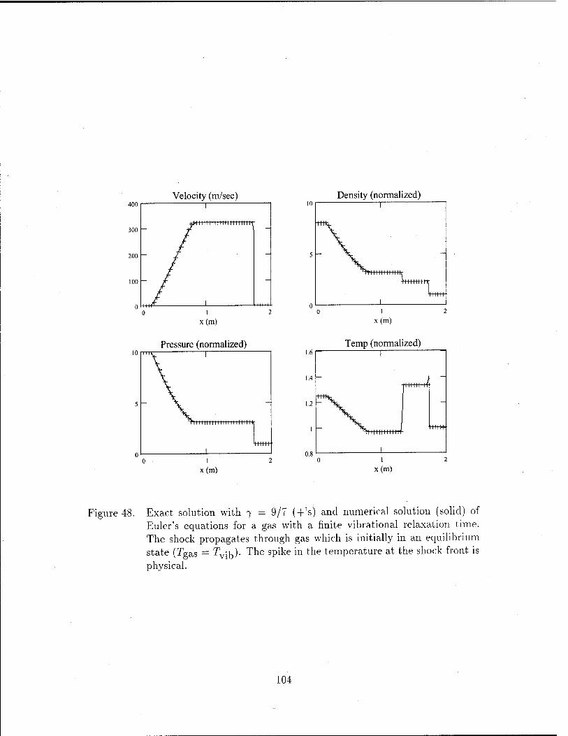
400 Velocity (m/sec)

300 -

200 -

mi iniiiiiiMi nut

_L

x(m)

Pressure (normalized)

x(m)

Density (normalized)

1.6

1.4

1.2

> L11111 11 K

x(m)

Temp (normalized)

HIHIHI'

11111111 It mm-

x(m)

Figure 48. Exact solution with 7 = 9/7 (+'s) and numerical solution (solid) of Euler's equations for a gas with a finite vibrational relaxation time. The shock propagates through gas which is initially .in an equilibrium state (Tgas = Tvj^). The spike in the temperature at the shock front is physical.

104

A close-up of the vibrational and gas temperature profiles in the shock front

region is shown in Figure 49. The gas temperature (solid) initially rises rapidly at

5 a 1) a. B

4M) 1 1 i i i

4UU

\

350

i

i i

JOi)

i i i

1.6 1.65 1.7 1.75 x(m)

1.8 .85

Figure 49. Gas temperature (solid) and vibrational temperature (dashed) in the shock front region for a shock propagating through gas in an equilibrium state.

the shock front to a value of 420K, then decreases gradually in the post-shock region

to a temperature of 400A" as energy is taken from the flow and transferred into the

vibrational modes. These post-shock temperatures are precisely those values pre-

dicted based on the Rankine-Hugoniot relations for a gas with a 7 of 7/5 and 9/7,

respectively, at a shock velocity of 571 m/sec. Due to the finite vibrational relax-

ation time, the vibrational temperature (clashed) rises gradually in the post-shock

region until the vibrational and translational/rotational modes achieve equilibrium.

The peak in the gas temperature corresponds precisely to the analytically predicted

temperature just behind the shock front for a gas with a 7 of 7/5 (i.e., a gas with

no vibrational modes). The equilibrium temperature corresponds precisely to the

analytically predicted temperature in the post-shock region for a gas with a 7 of 9/7

(i.e., full equilibration between translation, rotation and vibration). Longer vibra-

tional relaxation times result in a spike with a wider spatial width and vice-versa.

105

As mentioned previously, the value of the relaxation time constant .(r) used in this

calculation was equal to 20 times the value of the time step used in the integration of

the fluid equations {At). Therefore, the vibrational relaxation length shown in Fig-

ure 49 is not independent of the grid resolution. However, the peak gas temperature

and the final equilibrium temperature are independent of the grid resolution.

100 150 Distance (cm)

Figure 50. Numerically (solid) and analytically (dashed) determined shock velocity for the Riemann problem in which the shock propagates through gas with a finite vibrational relaxation time. The gas is initially is an equilibrium state.

As previously mentioned (Chapter III), the shock speed is another indicator

of the quality of the numerical solution, although it is not one of the variables di-

rectly obtained in the integration of the fluid equations. The shock speed can be

determined by tracking the spatial position of the shock front {? shock) in time {t),

then calculating the derivative of the trajectory from Vskock = dxsh0ck/dt. Further

details regarding the numerical determination of the shock speed are given in Ap-

pendix B. A comparison between the shock speed determined analytically (dotted)

and numerically (solid) is shown in Figure 50. Here, the shock speed determined

numerically is within approximately 0.5% of the analytic value (571 m/sec). The

106

small oscillations in the shock speed have an amplitude of less than 2 m/sec and are

caused (primarily) by the uncertainty with which the position of the shock front is

known at any instant in time. That is. the shock front position at any time is known

numerically only to within the spatial resolution of the solution, which is the interval

between adjacent nodes.

In this validation, the shock propagated into gas that was initially in an equi-

librium state. Both the flow parameters in the shock front region and the shock

velocity were found to be in good agreement with analytic values. In the next sec-

tion, a shock will be propagated into gas that is initially in a nonequilibrium state.

This is representative of the nonequilibrium conditions that may be present in a

neutral gas clue to the presence of a weakly ionized plasma,

4.2.3 Numerical Results. In this section, the experimental arrangement

depicted in Figure 47 will be modeled as shown in Figure 51. Here, a shock tube is

used to generate a shock, which then propagates into a gas with a nonequilibrium

store of vibrational energy. The low pressure side of the shock tube is divided into

High Pressure (P4)

T =T x gas vib

equilibrium region

Low Pressure (Px)

T =T 1 aas vib

equilibrium region

T <T u x gas * vib

nonequilibrium , region

Figure 51. Shock tube used to model the nonequilibrium vibrational relaxation effects. The pressure is continuous throughout the low pressure side of the shock tube.

two regions: an equilibrium region and a nonequilibrium region. The equilibrium

region is characterized by Tvib = Tgas and represents the region through which a

shock would propagate in the absence of a plasma, as depicted by the left half of

10<

Figure 47. The nonequilibrium region is characterized by Tvlb > Tgas and represents

the plasma region into which the nominal shock propagates, as depicted by the right

half of Figure 47. As the shock front passes into the nonequilibrium section, the

excess vibrational energy is released into the post-shock region. As this energy is

transferred to the other modes, it heats the gas. It will be shown that this release

of energy will accelerate the shock wave to a higher velocity.

The shock tube used in this nonequilibrium example is the same as that used in

the code validation (200 cm long with a diaphragm located at 80 cm). An equilibrium

region (characterized by equal gas and vibrational temperatures of 300A") will extend

20 cm to the right of the diaphragm, with an abrupt transition to a nonequilibrium

region (characterized by a vibrational temperature of 600A' and a gas temperature of

300A') at 100 cm. The vibrational energy corresponding to a vibrational temperature

of 600 A, as used in Equation 73, is equivalent to the vibrational energy corresponding

to a vibrational temperature of approximately 1700 A, as used in the usual definition

of specific vibrational energy (Equation 35). Since a vibrational temperature of

1700A" is considered typical of that encountered in a glow discharge in N2, the

present use of a vibrational temperature of 600A' is understandable. When the

diaphragm bursts, the shock forms and propagates at a velocity of 571 m/sec in

the equilibrium gas, as in the validation case previously discussed. The minimum

steady-state shock velocity {VCj), defined by the Chapman-Jouguet point (Chapter

II), under these conditions is 550 m/sec. Since the shock velocity will enter the

nonequilibrium region with a velocity greater than VCJ, no acceleration is expected

according to the common interpretation of the theory [27].

The numerical solution obtained under the given nonequilibrium conditions

is shown in Figure 52. The shock structure observed in this nonequilibrium case

is quite different from that observed in the equilibrium case. In the equilibrium

case, the density and pressure in a fluid element increased as the fluid element was

transported from the point just behind the shock front to the post-shock equilibrium

108

400

200

Velocity (m/sec)

*-^ i

x(m)

Pressure (normalized)

10

5 -


^ j

x(m)

Temp (normal ized) l.b I -" -\

1.4 -

1.2 -

1

1

—

x(m) x(m)

Figure 52. Numerical solution of Euler's equations for a gas with a finite vibrational relaxation time. The shock propagates through gas which is initially in a nonequilibrium state (Tgas = 600A',Tv^ = 300A).

region (Figure 48). In the nonequilibrium case, the density and pressure in a fluid

element decrease as the fluid element is transported from the point just behind the

shock front to the post-shock equilibrium region. In addition, in the equilibrium

case the gas temperature rises sharply across the shock front, then decreases as

equilibrium is approached. In the nonequilibrium case, the gas temperature rises

sharply across the shock front, then continues to rise as equilibrium is approached.

The vibrational and gas temperature profiles in the shock front region are

shown in Figure 53. Here the gas temperature (solid) rises sharply across the shock

109

E i-

/OO

600

500

1 1 1

/ /

/ / -

400

1

-

JUO 1 1.6 1.7

x(m)

Figure 53. Gas temperature (solid) and vibrational temperature (dashed) in the shock front region for a shock propagating through gas in a nonequilibrium state.

front to a value of approximately 450Ä', then rises more gradually until equilibrium

is achieved at a temperature of approximately 480Ä'. The vibrational temperature

(clashed), on the other hand, decreases gradually until equilibrium is reached. In

this case, energy is transferred from the vibrational modes into the translational

and rotational thermal modes. This energy transfer heats the gas and increases

the pressure in the equilibrium region above the equilibrium value obtained in the

previous case. The increased pressure, in turn, causes the shock front to accelerate

to a higher velocity.

The variation in the numerically determined shock velocity with distance is

shown in Figure 54 (solid). The shock accelerates rapidly upon entering the nonequi-

librium region, even though the initial shock velocity (571 m/sec) is greater than

VCJ-, the minimum steady-state velocity (550 m/sec). This is an apparent contradic-

tion to the commonly reported understanding of nonequilibrium shock theory. The

dashed line shown in Figure 54 is an analytic prediction of the new steady-state

shock speed in the nonequilibrium region. The numerically determined shock speed

110

80 100 120 140

x(cm)

Figure 54. Numerically determined shock velocity (solid) for the Riemann problem in which the shock propagates through gas initially in both equilibrium and nonequilibrium states. The shock velocities under equilibrium (dotted) and nonequilibrium (dashed) conditions are analytically determined. The velocity according to the Chapman-Jouguet regime is 550 m/sec. The nonequilibrium region starts at 100 cm.

is observed to converge to within 0.2% of the analytic value. The derivation of the

analytic prediction of the shock speed in the nonequilibrium region of the shock tube

is the subject of the next section. The time (distance) required to achieve the new

steady-state shock velocity depends on the characteristic vibrational relaxation time

(distance). If this time is short, then the energy is transferred quickly between the

various modes and the shock speeds up quickly. If this time is long, then the transfer

of energy takes place slowly. Independent of relaxation time, however, the eventual

steady-state shock speed converges to the same value.

4.24 Analytic Determination of Shock Speed. According to the theory

of shock propagation in nonequilibrium gases as discussed by Osipov, et al. [93],

which is based on the work of Landau [79] and Zel'Dovich [123], a shock propagating

into a medium at a velocity less than the minimum steady-state shock velocity, VCj

111

(defined by the Chapman-Jouguet point as discussed in Chapter II), will accelerate

until its velocity matches the minimum velocity; i.e., the shock will accelerate until

the downstream equilibrium flow conditions match those at the Chapman-Jouguet

point. Osipov's theory does not predict acceleration beyond VCJ. A shock entering a

nonequilibrium region with a velocity equal to or greater than VCj is also unacceler-

ated according to Bystrov, et al. [27]. It was observed that the computational results

from the present work did not support these claims in all cases. Computationally,

shocks with initial velocities below some value, Vcrit (where Vcr!t < \CJ), accelerated

to a steady-state velocity equal to VCj- in accordance with previous theory. How-

ever, shocks with initial velocities greater than Vcrit were observed to accelerate to

steady-state velocities greater than VCj, in apparent contradiction with the theory.

In addition, shock acceleration occurred even when the initial shock velocity was

greater than VCj, also in apparent contradiction with theory. It will be shown in

this section that the present numerical results are correct and that the previous un-

derstanding of the theory describing shock propagation in nonequilibrium gases has

been either incomplete or incorrect.

The foundation for the analytic determination of the steady-state shock ve-

locity in the nonequilibrium region rests on Emanuers development of the solution

to the Riemann problem [40:181-183]. Here, his notation is adopted and his devel-

opment refined to apply to nonequilibrium conditions. Emanuers development of

the Riemann solution is followed precisely up to lite point just beyond his equation

(10.2), with the chief result being

C'A

where C is the speed of sound, U is the flow velocity in the laboratory frame and

the subscripts 4 and 5 refer to the region of undisturbed high pressure gas and the

region between the contact surface and expansion fan, respectively. This equation

112

assumes that the flow between these two regions is isentropic, which is the case in

nonequilibrium relaxation as well, since the nonequilibrium gas will always be to

the right (upstream) of the original contact surface (Figure 51). The pressure and

velocity are continuous across the contact surface, thus P5 = P2 and V5 = V2. Using

this in Equation 74 and writing P2/P1 as (Pj/P^/qPi/Pi) results in

P2 PA fl4 ~l\ U2] *74

74-1

Px ' " Pi 1 — { 2 JcJ

where the subscript 1 denotes the undisturbed region in front of the shock and the

subscript 2 denotes the region between the shock front and the contact surface.

Equation 75 is the starting point for the extension of the analytic solution to the

nonequilibrium cases. It is important to understand that no assumptions have been

made regarding the equilibrium (or nonequilibrium) state of the gas in deriving

Equation 75.

In the usual Riemann problem, the known parameters are the pressures on

either side of the shock tube diaphragm (P4 and Pi), the speeds of sound on either

side of the diaphragm (C'4 and C\) and the gas types on either sides of the diaphragm

(74 and 71). Thus, the unknown variables in Equation 75 are the pressure ratio at the

shock front (P2/Pi) and the flow velocity of the gas just behind the shock front (U2).

The usual approach to the problem then uses the Rankine-Hugoniot relations (which

describe the relationship between shock Mach number and either pressure, density

or flow velocity ratios at the shock front) to write Equation 75 as a transcendental

equation with one unknown parameter. The solution is then determined by finding

the root to Equation 75. Once this value is known, the shock velocity, pressure

ratio at the shock front (P2/P1) and the flow velocity behind the shock {U2) are all

determined. In this approach to the problem, a gas in initial equilibrium has been

assumed. Where was this assumption made? It was made implicitly in the use of

the Rankine-Hugoniot relations, which were derived for a gas in initial equilibrium.

113

The shock adiabatics (discussed in Chapter II) could have been used (instead

of the Rankine-Hugoniot relations) to find the root of Equation 75. In this case, the

shock adiabatic corresponding to the final state of the gas (Equation 36) is used in

conjunction with a line of constant mass flux, which defines a shock velocity. The

intersection of these two curves then determines both the pressure ratio (P2/Pi) and

the flow velocity in the equilibrium region behind the shock front (U2) (see Figure

21). In this figure, the equilibrium region is defined as the point B. The pressure

ratio at this point (P2/Pi) can be read directly off the curve, while the flow velocity

at this point can be determined from the principle of conservation of mass flux (in

the shock front frame) by

where UB is flow velocity at the equilibrium point in the laboratory frame, V is the

specific volume and P is the pressure. In the present notation. Equation 75 can be

written as PR PA f74~l> UB]

274 74-1

PI PI 1 —

{ 2 J cü\ where the subscript B has replaced the subscript 2 in denoting the equilibrium region

behind the shock front, consistent with the notation previously adopted. Thus,

numerically, the problem becomes one of just finding a constant mass flux line with

the correct slope (shock velocity) such that the flow parameters at point B satisfy

Equation 77.

The same thing can be done for the case in which the gas is initially in a

nonequilibrium state, except that the shock adiabatic is given by Equation 36 with

Tvibl ^ Tga.Sl ■ Equation 75 remains valid, with the unknown parameters still being

P2/Pi and U2- Both of these unknowns can be found by finding the intersection

(point B) of the constant mass flux line (Equation 76) with the equilibrium state

adiabatic (Equation 36) such that the flow parameters at point B satisfy Equation

114

77. Thus, a simultaneous solution of three equations is required. This is exactly

what was done in the equilibrium case, with Tvibl = TgaSl in Equation 36.

800

>

700-

600-

500

1 1 1 1 ,

0 / y /

* /

ja / / / /

/

1

/ /

45°

1 1 1 400 500 600

V(.„ (m/sec) 700

Figure 55. Variation of the steady-state shock velocity {Vss) in the nonequilibrium region with the entrance shock velocity {Vin). The conditions in the nonequilibrium region remain fixed (T^ = 600A", Tgas = 300A', P = 760 torr). Shown are the shock velocity determined by the fluid code (boxes), by the nonequilibrium extension to the Landau/Zel'Dovich theory (solid) and by the old theory (clashed). The shock velocity corresponding to the Chapman-Jouguet condition is 550 m/sec.

Comparisons of the shock speeds determined by the different methods are

shown in Figure 55. The numerically determined steady-state shock speed in the

nonequilibrium region (boxes) agrees very well with the results from the present an-

alytical method (solid curve), with relative errors between the two less than 0.2%

under the present conditions. The commonly understood application of the clas-

sical theory is also shown (dashed). The shock velocity as the shock enters the

nonequilibrium region (Vin) is plotted along the ordinate, while the steady-state

shock velocity in the nonequilibrium region (Vss) is plotted along the abscissa. In

all cases, the nonequilibrium region was characterized by a vibrational temperature

of 600A, a gas temperature of 300A' and a pressure of 760 torr. This defined a

115

minimum steady-state velocity {VCJ) of 550 m/sec. corresponding to the Chapman-

Jouguet point. The classical theory predicts that for cases in which \]n < VCJ, the

steady-state velocity should be equal to VCJ. For cases in which Vin > VCJ, the

steady-state velocity should equal Vtn. The present theory predicts a steady-state

shock velocity equal to X'CJ only for shocks entering the nonequilibrium region with

a velocity less than a certain critical shock velocity, Vcrit, where Vcrit < VCJ-

The value of Vcrtt can be determined by using Equations 76 and 77. The mini-

mum steady-state shock velocity that allows a fluid element to reach the equilibrium

region is given by \'cj. Taking the point B to be equal to the point CJ (see Figure

25), these equations become

where UCJ is flow velocity at the Chapman-Jouguet point in the laboratory frame,

V is the specific volume and P is the pressure and

PA PC •J

Pi Pi

74 - 1\ UCJ

CA\

114 ■-,4-1

where the last equation has been rewritten by solving for PA/PI- Since the known

nonequilibrium initial conditions (Vu Pi,Tvibl) define the Chapman-Jouguet point

{PCJ^VCJ), the initial pressure ratio {PA/Pi) is determined. The shock velocity cor-

responding to this pressure ratio defines Vb, which is an entrance velocity threshold.

A shock entering the nonequilibrium region below this threshold will accelerate un-

til the steady-state velocity is equal to the Chapman-Jouguet velocity (VCJ). A

shock entering the nonequilibrium region with a velocity in excess of Vcrit will have a

steady-state velocity greater than VCj. For the parameters corresponding to Figure

55, Vera, (determined by Equations 78 and 79) corresponds to 445 m/sec, which is in

excellent agreement with the numerical results shown in this figure.

116

It has been reported by Bystrov, et al. [27] that the velocity of a shock in a

plasma depends on the velocity of the shock as it enters the plasma, the properties

of the plasma ahead of the shock front and the processes which occur behind the

shock front. Bystrov suggests that the post-shock release of nonequilibrium vibra-

tional energy cannot explain the observed shock variations in his experiment, based

on his belief that the steady-state shock velocity in such cases is determined by the

Chapman-Jouguet velocity. The results obtained in the present investigation sug-

gest that this belief is incorrect. As Figure 55 clearly shows, the final steady-state

shock velocity depends on the velocity of the shock as it enters the nonequilibrium

region. In addition, this velocity depends on Tvtbl, which varies with differing plasma

conditions in front of the shock. Finally, although full vibrational/translational equi-

libration was assumed in the present calculations, such need not be the case. For

cases in which only part of the nonequilibrium vibrational energy is released, the

shock velocity in the nonequilibrium (plasma) region will be less than that obtained

assuming full equilibration (i.e., the shock velocity depends on the processes which

occur behind the shock front). Therefore, the shock velocity behavior resulting from

nonequilibrium vibrational relaxation is consistent with all of the qualitative obser-

vations reported by Bystrov.

Hi

4.3 Analysis of Vibrational Kinetics

In the previous section it was shown that it is possible, in principle, for nonequi-

librium vibrational energy relaxation to increase the shock speed. In practice, how-

ever, two conditions must be satisfied in order for this to occur. First, an appreciable

amount of energy must be extracted from the vibrational mode in the post-shock

region. Second, this energy must be extracted quickly. In the calculations of the

previous section, both of these requirements were met. However, both the amount

of vibrational energy available for extraction and the time constant (r) at which this

energy was released were chosen without regard as to the physical properties (or lim-

itations) of an actual molecular gas. Rather, the intent of the previous calculations

was to examine the influence of vibrational energy relaxation given a gas which met

both requirements. In the present section, the ability of an actual gas to met the

stated conditions will be examined.

Pure molecular nitrogen will be used as the test gas in this analysis of the

vibrational kinetics. This choice was made based on the availability of experimental

data taken in pure N2 gas. In addition, since N2 comprises nearly 80% of air, the

substance through which all aerodynamic vehicles must fly, it seems reasonable to

use this gas as a starting point. In reality, of course, air is not made of pure molecular

nitrogen, but has many other constituents which can change the kinetic rates upon

which the present study is based. However, it will be assumed that air can be

simulated by pure molecular nitrogen well enough to permit order of magnitude

calculations of the relevant parameters.

4.3.1 How Much Energy Can Be Released? The maximum amount of

nonequilibrium vibrational energy which can be added to the flow in the post-shock

region depends on two things. These are the amount of energy initially contained in

the vibrational manifold for the gas in front of the shock and the amount of energy

contained in the vibrational manifold for the gas at equilibrium in the post-shock

118

region. The difference between these two is the energy added to the flow. In order

for vibrational energy relaxation to lead to significant variations in the flow field,

the amount of energy added to the flow behind the shock front must comprise an

appreciable fraction of the thermal energy already present in the flow in the post-

shock region (estimated to be approximately 10% or more).

o Tvib=Tgas=804K

Tgas=300K x

30 45 V level

60

Figure 56. Nonequilibrium (dashed) and equilibrium (solid) vibrational distribution functions in N2. The nonequilibrium distribution is representative of that obtained in a glow discharge plasma, while the equilibrium distribution is representative of that obtained in the equilibrium region downstream of a Mach 3 shock. The amount of energy added to the flow per molecule is approximately equal to the difference between the average energies of these two distributions.

As an example, consider the two vibrational distribution functions (VDFs)

shown in Figure 56. Here, a nonequilibrium VDF (clashed), representative of condi-

tions within a weakly ionized yV2 plasma region, can be compared to an equilibrium

VDF (solid), representative of conditions in the equilibrium region behind a shock

front. The average specific vibration energy corresponding to the nonequilibrium

VDF is approximately equivalent to the specific vibrational energy given by the

Equation 73 with a vibrational temperature of 600A'. The nonequilibrium VDF

119

shown here was calculated by solving the coupled set of rate equations for each vi-

brational level of Ar2 until a steady-state solution was obtained. The calculations

were performed using the same vibrational kinetics code discussed in Chapter II

[35]. The electron impact excitation of ground state molecules normally present in

a weakly ionized plasma was simulated in the rate equations by an excitation rate,

R N0 (Equation 39), which serves as a pump. This pump promoted ground vibra-

tional state molecules (i'=0) to the first excited state (i>=l) at a constant frequency

(v is the vibrational quantum number). The nonequilibrium VDF in Figure 56 is

characterized by a vibrational temperature, T™b, of 1900A, where T™ is based on

the relative populations of the v=0 and v=l state. The calculation assumed gas at a

pressure of 760 torr (1 atm) and a gas temperature of 300A". The equilibrium VDF is

a Maxwell-Boltzmann distribution with a characteristic temperature of 804A", which,

by the Rankine-Hugoniot relations, is the gas temperature just behind the shock for

a Mach 3 shock in N2. The maximum amount of energy per molecule which can

be extracted from the nonequilibrium VDF and added to the flow is the difference

between the average energies of these two distributions. Shocks with higher (lower)

Mach numbers will produce higher (lower) post-shock gas temperatures, resulting in

equilibrium distributions with a higher (lower) average energy than the one shown in

Figure 56. This leads to less (more) vibrational energy added to the flow for a given

nonequilibrium VDF. Likewise, higher (lower) pumping rates lead to nonequilibrium

VDFs with higher (lower) average energies, which allow more (less) energy to be

added to the flow for a given shock velocity.

The maximum amount of energy available for extraction per molecule can be

estimated by subtracting the average vibrational energy at equilibrium (approximat-

ing the equilibrium gas temperature in the post-shock region as the gas temperature

just behind the shock front) from the average steady-state nonequilibrium vibrational

energy: Anoneq eq /Qf\\ e = e1

H — e2 , (oO)

120

where tnoneq is the average energy of the steady-state nonequilibrium vibrational

distribution and eeq is the average energy of the equilibrium vibrational distribution.

The subscripts 1 and 2 refer to the regions in front of and behind the shock front,

respectively. The energy difference calculated from Equation 80 can be normalized

by the specific energy initially present in the translational and rotational modes at

the post-shock gas temperature {T2):

thermal 1 kB T<

7-1 M (si:

As stated previously, significant alterations to the flow field are estimated to occur

when the amount of energy added to the flow is approximately 10% (or more) of the

thermal energy already present in the flow.

-a N

O

to <

80 1 1 1 \ 4

60 M = 2/

40 / M = 3/_

20 - /^ s^ yS -

^^ ^^-^M = 5^

II

i l 1

500 1000 1500 2000

Figure 57. Maximum amount of vibrational energy (estimated) available for release into the post-shock region at four Mach numbers (shown as a % of the thermal energy initially present in the post-shock region). Energy flows from the vibrational modes to translation/rotation for positive values, and from translation/rotation to vibration for negative values.

An estimate of the maximum amount of nonequilibrium vibrational energy

available for release into the flow behind a shock has been determined over a range

121

of conditions which are realistically achievable in a glow discharge plasma (Figure

57). Here, steady-state nonequilibrium VDFs characterized by vibrational tempera-

tures (Tj°6) from 300A' to 2000A' were calculated in ;V2 at a pressure of 1 atm and

a gas temperature of 300A'. Positive values indicate that in order to reach equilib-

rium behind the shock front, energy will flow from the vibrational modes into the

translation/rotation modes. Negative values indicate that the reverse is true. As the

shock Mach number rises, so does the post-shock equilibrium gas temperature. Thus,

what was a vibrational energy source at one Mach number can become a vibrational

energy sink at a higher Mach number, all else being equal.

The vibrational energy represented in Figure 57 is the maximum amount of

energy available for release at a given T™b and shock speed. How much of this energy

is released depends on the time scale of interest. If the time scale of interest is very

long, nearly all of the energy can be released, while if the time scale is short, very

little may be released. How much vibrational energy can be released on a given time

scale is the subject of the next section.

4.3.2 How Fast Can the Energy Be Rekastdi In shock/plasma experiments

conducted to date with molecular gases, the experimental shock tubes are of the or-

der of 1 meter in length. Therefore, for the present analysis, the time scale of interest

will be the time it takes a shock of a given velocity to travel a length of 1 meter.

How much vibrational energy can be released into the flow during this time depends

on the kinetic rates of the vibration-vibration (XX) and vibration-translation (VT)

energy exchange processes. The temporal release of nonequilibrium vibrational en-

ergy, properly accounting for the VV and \'T energy exchange mechanisms, was

investigated with the use of the same vibrational kinetics code used previously to

calculate the steady-state nonequilibrium YDFs.

A steady-state nonequilibrium vibrational distribution function with realistic

parameters was used to represent the vibrational state of the gas in front of the shock

122

(T^b = 1900A'. Tga, = 300A", pressure = 1 atm). The passage of the fluid element

across the shock front was simulated by the increase in density and gas temperature

consistent with the Mach number of the shock. The increase in density and gas

temperature behind the shock lead to an increase in the VT rates, which results in

the release of vibrational energy into the flow. The amount of this energy release was

tracked throughout the time-dependent calculation, with the result shown in Figure

58 for a Mach 4 shock in N2- In this case, the maximum amount of vibrational

time (msec)

Figure 58. Amount of vibrational energy added to the flow (shown as a % of the thermal energy initially present in the post-shock region) for a Mach 4 shock in iYr

2. The initial nonequilibrium vibrational distribution (T™b = 1900A') was calculated for a gas at a temperature of 300A' and a pressure of 1 atm.

energy which can be released into the flow is approximately 18% of the thermal

energy initially present in the post-shock region (see Figure 57). A Mach 4 shock

(traveling in 300A' gas) can travel 1 meter in a time of 0.71 msec. In this time,

an amount of vibrational energy equal to approximately 10% of the thermal energy

initially present in the post-shock region can be released. This is the amount of

energy estimated to begin to cause interesting effects in the flow. It is seen from

123

Figure 58 that, under the present conditions, the maximum amount of energy will

be released into the flow in approximately 4 msec.

For a given nonequilibrium vibrational distribution, there appears to be an

optimum shock speed which defines the conditions under which the most vibrational

energy can be extracted and released into the flow behind a shock. A shock with a

low Mach number will take the longest time to traverse a given distance, therefore

providing more time during which energy will be extracted from the vibrational

manifold. However, the low Mach number also produces low gas temperature and

density jumps across the shock front, resulting in a long vibrational relaxation time

constant (re£r), since refj is inversely proportional to both density and VT rates (VT

rates increase with increasing gas temperature, as shown in Figure 26). Therefore,

although more time is available during which energy release can occur, the amount

of energy released on the time scale of interest is small. On the other hand, shocks

with high Mach numbers will have high density and temperature jumps, resulting in

shorter reffs and a quicker energy release. However, the higher shock speed means

that there will be less time during which the vibrational energy can be extracted. In

addition, the higher post-shock temperatures from the fast shocks result in higher

initial post-shock thermal energies. Thus, although the vibrational energy can be

extracted quickly, its relative contribution to the total thermal energy in the flow

may be minor.

4-4 Conclusion

The release of excess vibrational energy in the post-shock region results in

increases in the shock speed. Assuming that full equilibration among the various

thermal modes (translation, rotation, vibration) is achieved in the post-shock re-

gion, an analytic expression has been derived, from which the shock speed in the

nonequilibrium region can be determined for a Riemann shock problem. This ana-

lytic solution agrees well with results from a numerical solution to Eulers equations,

124

many of the plasma/shock experiments reported in the literature were conducted in

air, this may have been the case. However, while the increased VT rates would reduce

the vibrational energy transfer time, they would also reduce the amount of energy

contained within the vibrational manifold. So although the vibrational energy could

be transferred quicker, there would be less energy to transfer.

To further study the quantitative effects of nonequilibrium vibrational energy

transfer, a more detailed fluid approach would be required. In this refined study, each

vibrational level should be treated as a separate gas. Taking into account the VV

and VT energy exchange processes in this manner would eliminate the need for an

effective relaxation time constant (r), as used in the present analysis. Thus, the vari-

ations in flow parameters and shock speed could be more accurately tracked, leading

to a more refined assessment of the role of nonequilibrium vibrational relaxation.

Although the focus of this chapter was on post-shock energy addition in the

form of nonequilibrium vibrational relaxation, one cannot ignore the fact that the

shock phenomena which have been observed in molecular gases have been observed in

atomic gases as well ([33], [12] and [41], for example). Since such gases obviously lack

vibrational degrees of freedom, some other mechanism must be at work. Although

it is true that a weakly ionized plasma in an atomic gas may have processes such as

de-excitation of electronic states and recombination ongoing, the low number density

of the relevant species argues against these mechanisms being sufficiently strong to

account for the observed variations in shock velocity and shock structure.

126

V. Thermal Effects

5.1 Introduction

Anomalous behavior has been observed as a shock propagates through a plasma,

This behavior has not been observed when the shock propagates through a homo-

geneous neutral gas at a fixed temperature. In the shock experiments conducted

in a plasma, it is difficult to completely avoid heating of the neutral gas. That is.

experimentally it is difficult to create a plasma that does not heat the neutral gas.

Alternatively, one could try to heat the gas without creating a plasma (by the use

of a hot Ni-Cr wire placed down the tube centerline, for example). However, such

attempts may have difficulty in obtaining the same peak temperatures and/or a sim-

ilar radial temperature profile as observed when the heating is due to the plasma.

Another complication possibly introduced by this method is the presence of the as-

sociated heating apparatus in the shock tube, which may affect the gas flow and

complicate measurements of density, pressure, etc. In an attempt to isolate plasma

effects from thermal heating effects, pulsed discharges have been used. These devices

produce a plasma over a short temporal duration, with the premise being that the

neutral gas temperature doesn't change much during this time. However, difficulties

arise in the analysis of such pulsed devices due to the transient nature of the plasma.

A steady-state glow discharge is a much simpler system to analyze due to the absence

of significant variations in the plasma parameters.

Shock characterization and modification are conveniently classified according

to the method of initiating the shock. There are two common methods used to

generate a shock. The first uses a classical shock tube arrangement in which a

breakable diaphragm separates high and low pressure gas. When the diaphragm is

ruptured, the gas flows from high to low pressure, producing a shock in the process.

The experimental apparatus which produces a shock in this manner is commonly

called a shock tube, while the theoretical analysis of this problem is commonly

127

called the Riemann (or shock tube) problem [61]. The second method uses a burst

of energy to locally heat the gas in a small region of a tube. This heating leads to a

local increase in the pressure, which causes the gas to flow to regions of lower pressure.

The burst of energy is typically due to the discharge of an electrical capacitor. This

method of impulsively generating a shock is called a spark-initiated shock. A typical

Electrode

Shook wave / 7

Plasma-heated ( neutral gas j

Figure 59. Typical experimental arrangement in which a shock propagates into a plasma-heated gas.

experimental arrangement is shown in Figure 59. in which a shock (produced by a

spark discharge, as shown in this example) propagates into a plasma. A steady-

state glow discharge of limited spatial extent heats the neutral gas. In general,

the temperature of the gas throughout the heated region (and in the absence of a

shock) will be a function of position and time (i.e.. T = T{r,9,z,t), in cylindrical

coordinates). In the present analysis, symmetry in the 9 direction and steady-state

conditions will be assumed, thus T = T(r.: I. A shock is produced and propagates for

some distance in ambient gas before it enters the region containing the hot gas. Any

modifications to the shock due to the presence of t hermal inhomogeneities are termed

thermal effects. Although the plasma is comprised of ions, electrons and neutral

gas particles, the relative fraction of the charged specie are very small. Typical

ionization fractions in a glow discharge plasma are in the range 10-6 - 10-8 [98:3]

(i.e., approximately one electron/ion pair for every ten million neutral gas particles).

128

The minority of electrons and ions in the flow was the basis for the conclusion in

Chapter III that charged particles have an insignificant effect on the shock.

In this chapter shock modification due to thermal inhomogeneities will be ex-

amined using a two-dimensional computational fluid dynamics code written for this

purpose. This code simulates both the Riemann problem and the spark-initiated

shock problem, each of which has been used in shock propagation experiments in-

volving a plasma. Code details are given in the next section and in Appendix B.

Results will be presented which validate this code for both types of problems. The

code will then be used to study thermal effects on shock propagation, beginning

with a simple thermal discontinuity. A more general class of two-dimensional ther-

mal inhomogeneities is then treated and related to glow discharge conditions. The

assessment of thermal effects concludes with simulations of and comparisons to ex-

periments conducted by both Western [46] and Russian ([115], [52]) researchers.

5.2 Model Equations

The model equations used in this analysis are the two-dimensional Euler equa-

tions. These four equations (conservation of mass, conservation of x momentum,

conservation of y momentum and conservation of energy) are augmented by a fifth

equation in the case of a spark-initiated shock. This last equation is used to describe

the physical process of energy from the spark discharge coupling into the neutral

gas. This equation governs the temporal and spatial release of energy into the flow,

thereby producing a shock wave similar to that produced by a spark source. The

form of this equation is very similar to that used to describe either the release of

vibrational energy or the detonation of chemical energy in the flow. The latter anal-

ogy is adopted as the model describing the generation of a spark-initiated shock.

Accordingly, the fifth equation expresses the principal of conservation of chemical

energy. In the case of a Riemann (or shock tube) problem the use of a conservation

of chemical energy equation is not required.

129

The equations used to model the flow can be written as [62:69]

dU ÖE OF -. , -

at ox oy (82)

where U is the vector of conserved quantities, E and F are flux vectors, H is a vector

of sources due to axisymmetric geometry and Q is a vector of sources describing

energy addition to the flow for a spark-initiated shock. Each of these vectors are

defined below. The coefficient a is 1 for two-dimensional axisymmetric geometry

and 0 for two-dimensional planar geometry, while the coefficient ß is 1 for a spark-

initiated shock problem and 0 for a Riemann problem. The vector of conserved

variables [U) is defined as

P

pVr

U= pVy (S3)

P{HV

?+ *?) + *¥} P^chem

where p is the mass density of the gas, Vx is the flow velocity in the x direction,

Vy is the flow velocity in the y direction, 7 is the usual ratio of specific heats, kß is

Boltzmann's constant, T is the gas temperature, M is the mass of the gas particle

considered, and tchem is the specific chemical energy to be used in generating a shock

in the spark-discharge case. Each of the variables in U is a function of x, y and t;

i.e., p = p{x,y,t), Vx = Vx(x,y,t), etc. The flux vectors E and F are defined as

pVx

p(K2 + ¥) E = pVxVy (84)

ptchem ^x

130

and

F =

PVy

pYxVy

p (v? + ¥)

PCchem^y

(So)

the axisymmetric source vector // is defined as

pVXVy

H pVf

Ptchem y'y

hile the vector of sources used for the spark-initiated shock problem is defined as

(86)

Q =

o

0

Pf-cher.

Plche

1ST'

where r governs the temporal release of the chemical energy. The first equation in

82 expresses conservation of mass, the second and third equations describe the con-

servation of momentum in the x and ij directions, respectively. The fourth equation

expresses the conservation of directed kinetic energy and thermal energy, where the

former depends on the mass flow velocity and the latter depends on the number of

degrees of freedom possessed by the gas particle under consideration and the gas

temperature. As an example of the latter, consider an Argon atom (7 = 5/3) which

possesses three degrees of freedom. With \kßT of energy per degree of freedom its

131

specific thermal energy is |^, which is equivalent to zpt^ff- The fifth equation

in 82 describes the conservation of chemical energy.

These equations were solved using an explicit MacCormack method [82] com-

bined with a flux corrected transport [23] algorithm. Strang-type splitting [109]

was used in order to extend the one-dimensional MacCormack algorithm to two-

dimensions. The source terms represented by the right hand side of Equation 82

were handled by an implicit method suggested by Yee [120:36]. Further details re-

garding the numerical solution of Equation 82 are given in Appendix B.

The MacCormack scheme (with second-order accuracy) was chosen clue to both

its suitability for solving nonlinear Equations [62:192] and its relative programming

ease. However, the use of a second-order accurate method by itself would lead to

oscillations in the solution near shocks. The FCT method was adopted as a way to

get rid of these numerical oscillations by preventing them before they are allowed

to grow [61:127]. Of course, other methods could be used to accomplish the same

goal (Godunov method, artificial viscosity, etc.), however the MacCormack/FCT

method offers stability and sharp resolution for a relatively small effort in coding

[112]. Higher-order Godunov schemes like the Roe method produce more accurate

solutions than the MacCormack/FCT scheme, however they are more complicated

to code and more expensive to run [44:173]. Additionally, the FCT method is more

accurate than using artificial viscosity to clamp out the oscillations [44:173].

5.3 Code Validation

5.3.1 Riemann Problem. The Riemann problem was solved numerically

in two-dimensional planar geometry for a shock tube with a length of 50 cm and

a half-width of 2.5 cm. The diaphragm was located at 20 cm with respect to the

high pressure end of the tube. The working gas was Argon with an initial pressure

ratio (P4/Pi) and temperature ratio (TA/Ti) of 10.0 and 1.25, respectively. The two-

dimensional calculation was performed on a grid with 401 nodes in the x direction

132

Velocity (m/sec) Pressure (normalized)

x(m)


x(m)

Temp (normalized)

\

1

1 Milt

i 0.2 0.4

x(m)

Figure 60. Analytic ( + ) and numerical (solid curve) solution to the Riemann problem (Argon with P4/Pi = 10.0, T4/7\ = 1.25).

(along the tube axis) and 23 nodes in the y direction (across the tube). A comparison

between the analytic solution to the Riemann problem (symbols) and the numerical

solution to the Euler equations (solid curve) along the shock tube centerline is shown

in Figure 60. In this figure, the values of pressure, temperature and density have

been normalized to the respective upstream ambient value. The agreement is quite

good, with relative errors in the pressure being less than 1% throughout the flow field

except at the leading and trailing edges of the expansion fan, near the contact surface

and near the shock front. The relative errors in these regions are typically less than

5%, with the relative error at one or two nodes very near the shock front being much

higher (« 50%). As discussed previously in Chapters III and IV, the higher relative

errors near the shock front can be attributed to the MacCormack/FCT method,

which smears this region over approximately 3 spatial nodes. In general, the relative

133

error throughout the physical domain can be reduced by increasing the number of

grid nodes in the computational domain, accompanied (of course) by an increase

in the computational requirements (memory, CPU time). Increasing the number

of nodes does not prevent the MacCormack/FCT method from smearing the shock

front region, however, thus the high relative error in one or two bins near the shock

front will remain high. 4

The transverse symmetry of the solution is illustrated in Figure 61, where

the full two-dimensional density (top) and pressure (bottom) solutions are shown.

The primary features of a Riemann solution are also shown in this figure. In this

figure, the tube centerline is along y - 0, while the tube wall is along the maximum

y coordinate in the domain. The solution is observed to be independent of the

transverse position, as it should be in this validation problem. The density and

pressure in these plots have been normalized by their respective upstream values.

4 Again, the barely discernable ripples in the numerical solution in the regions of the expansion fan and contact surface are due to the graphic conversion utility program used and were not present in the raw numerical data.

134

Density

shock front

Pressure

-,10

shock front

Figure 61. Density (top) and pressure (bottom) from the two-dimensional numerical solution to the Riemann problem (Argon with P4/P1 = 10.0, T4/T1 = 1.25). The density and pressure have been normalized to their respective ambient values.

135

20 25 30 35 40

Distance (cm)

Figure 62. Analytic (dashed) and numerically determined (solid) shock speed alon^ the centerline (Argon with P4/P1 = 10.0, TAjTx = 1.25).

The numerically determined shock velocity can also be compared to the an-

alytic value. This is useful because unlike flow velocity, density, temperature or

pressure, the numerical value of the shock velocity is not a direct output of the so-

lution to the fluid equations, as mentioned previously in Chapters III and IV. The

shock speed can be determined by the temporal evolution of the shock front po-

sition, as described in Appendix B. Figure 62 shows the analytically determined

shock speed (straight line) compared to the numerically determined shock speed.

The diaphragm is located at 20 cm, so that at time t=0, the shock speed is zero. It

is observed that the numerical shock velocity undergoes a transition period (lasting

about 200 jusec under the present conditions) during which it speeds up. overshoots,

undershoots, then converges to the proper analytic value. The analytic shock speed

(under the present conditions) is Mach 1.597, which is approximately equivalent to

515 m/sec when the ambient gas temperature is 300 K. The small oscillations in the

shock speed have an amplitude of less than 1 m/sec and are caused (primarily) by

the uncertainty with which the position of the shock front is known at any instant

in time. That is, the shock front position at any time is known numerically only to

136

within the spatial resolution of the solution, which is the interval between adjacent

nodes.

5.3.2 Spark-Initiated Shock. In the Riemann problem, the existence of an

analytic solution provides a useful tool to assess the quality of the numerical solution.

In contrast, no analytic solution is known to exist in the case of a spark-initiated

shock wave. However, since such initiation techniques have been widely used in the

study of shock propagation in plasma, it is necessary to be able to suitably simulate

the generation and propagation of a shock wave under such conditions. In this case,

the lack of an analytic solution forces a comparison of the numerical solution to

experimental observations in order to validate the code. Fortunately, observations of

sufficient detail have been made [37] that allow a comparison to take place, at least

qualitatively. Although the cited reference lacks many of the specifics necessary

for a full quantitative comparison, the general nature and behavior of the reported

observations are extremely valuable.

The spark-initiated shock is produced by discharging electrical energy across

a spark gap. This energy deposition begins when a sufficiently high voltage breaks

down the gas. The resulting plasma completes the electrical circuit and a current

flows through the gas (plasma) across the spark gap, heating the gas in the process.

As an example, consider an infinitesimal volume of gas. If a current flows through

this test volume then the gas is heated, while the number density in the test volume

initially remains constant. This results in a rise in the gas pressure within the test

volume. Consider another test volume of gas through which no current flows and

consequently does not get heated. Between the two test volumes a pressure gradient

is created which makes the fluid flow in the direction of lower pressure. If the heating

occurs quickly enough, then a pressure gradient is created with sufficient strength to

generate a shock wave.

137

The experimentally measured density distributions of a shock pulse generated

by a spark discharge at five instants in time (1.0, 1.7, 2.9, 5.6 and 9.8 /usec cor-

responding to curves 1, 2, 3, 4 and 5, respectively) are shown in Figure 63 (left),

taken from [37]. Notable features of the pulse are the spreading of the shock en-

velope and the accompanying decrease in amplitude as time increases. The shock

velocity is reported to be approximately 2000 m/sec at 'early times' (no specific

time is mentioned), with the corresponding temperature in the central region to be

approximately 40,000 K. In the experimental device of [37] a capacitor is used to

store the electrical energy prior to its release. This capacitor (0.25 /.if) is charged to

a voltage of 10 KV, resulting in an energy release of 12.5 Joules. The results of a

experiment simulation

Figure 63. Spark-initiated shock density profile: experiment (left, from [37]) and simulation (right)

numerical calculation simulating a spark-initiated shock pulse are shown in Figure

63 (right). The calculation times for the simulation correspond to the times in the

experiment. Although the numerical simulation does not reproduce the experimen-

tal density measurements exactly, the general behavior of the shock pulse is in fair

agreement with measurements. The numerical simulation generates a shock pulse

138

whose amplitude decreases, and whose pulse width increases with time, consistent

with experimental observations.

£

x

1

0 1 i i i i 1 1 1 1 1 1

O 9

a B I

Xi 6

ID 5

CO 4 ^ 3 - Ü o 2

_ ^ CO

1 Y, i i i i 1 , 1 1 1 1 ~

u 0 1 2 3 4 5 6 7 8 9 10 11 li

time (microsec)

2000

1500

1000 -

3 4 5 6 7

x (mm) 9 10

Figure 64. Variation of shock front position with time (left) from experiment (boxes) and from simulation (solid). Shock front speed (right) from simulation.

The position of the shock front as a function of time also closely replicates the

observed data (Figure 64 (left)). The slope of this curve at any point in space (time)

is the velocity of the shock at that same point in space (time). The simulated shock

velocity is shown in Figure 64 (right) as a function of position. At a time of 0.15

//sec, the simulation predicts a shock velocity of 1700 m/sec and a temperature at

the origin of 40,460 K, both in good agreement with reported values. The numerical

simulation used an energy release of 3.92 Joules (assuming a tube radius of 10 cm),

which is nearly a factor of three less than the energy released in the experiment.

However, this difference might be explained by the difference in pressures between

the simulation and experiment (30 torr in the simulation compared to an unknown

pressure in the experiment) or by a different shock tube radius (which was not

reported). Furthermore, some of the 12.5 Joules released in the experiment is lost

clue to radiation and does not heat the gas. Nevertheless, the favorable comparison

139

between the simulation and the experiment lead to the conclusion that the present

numerical method used to generate and propagate a shock pulse is representative of

spark-initiated shocks reported in the literature.

In addition to the validation tests discussed previously, in which the gas flow

was primarily along the computational grid lines (both Riemann and spark-initiated

spark problems), the code's ability to handle flows in general directions was tested.

In these tests, a square computational grid comprised of 151 nodes in each direction

(x,y) was used to simulate a physical domain of 10 cm by 10 cm. Both small-

amplitude and large-amplitude pressure disturbances were generated at the center

of the domain, simulating point explosions of various strengths. In the former case,

acoustic disturbances were observed to propagate radially outward from the center in

all directions at nearly equal velocities (within 3% of the acoustic velocity). Pressure

contours for this simulation are shown in Figure 65. Here, the small-amplitude wave

has propagated for a time of 1.188-4 sec in Argon at an ambient temperature of

300A'. Although the physical domain was represented on a Cartesian grid, the

resulting pressure contours are nearly circular, indicating the pressure disturbances

propagate at nearly equal velocities in all directions. If the pressure disturbance

originating at the origin is large, shock waves will form. For this case, shock waves

were also observed to propagate radially outward from the center in all directions, at

(again) nearly equal velocities (a 3% spread in shock velocities was noted). In both

cases, the slowest signal propagation speed occurred in angular directions that were

at 45 degrees relative to the computational grid lines.

140

0.05 x(m)

Figure 65. Pressure contours resulting from the propagation of a small-amplitude wave originating from the center of the domain (x = 0.05, y = 0.05). The velocity of the leading edge of the pressure disturbance in any direction is within 3% of the speed of sound.

141

5.-1 Step Temperature Rise

A sharp discontinuity in the temperature offers the simplest example of the

effects of a thermal inhomogeneity on shock characteristics. In this section, an infinite

planar interface will be considered which separates gas 1 at a temperature 7\ from

gas 2 at a temperature T2. The ratio of the heat capacity at constant pressure (Cp)

to the heat capacity at constant volume (Cv) (also known as the adiabatic exponent)

will be denoted as 71 for gas 1 and y2 for gas 2. A shock will be propagated from gas

1 through the thermal discontinuity into gas 2, with the resulting modifications to

the shock characteristics to be examined. Two cases will be considered. The first is

for the case in which T2 > Tu while the second is for the case in which the inequality

is reversed. The former case leads to transmitted shock and a reflected rarefaction

wave, while the latter case leads to both a transmitted and reflected shock [118:78].

5.4-1 Riemann Problem.

54.I.I Reflected Rarefaction Wave. A comparison of the calculated

pressure and density profiles obtained for the case in which T\ = 300A' and T2 =

600A" (solid) and the exact Riemann solution in which Ti = T2 = 300Ä' (clashed)

at the same instant in time is shown in Figures 66 and 67. The interface between

T2 and 7\ was initially located at x=35 cm. Although a heated region exists on

the low pressure side of the shock tube, the pressure remains constant in this region

(upstream of the shock front). This is representative of the steady-state condition in

a glow discharge in which the pressure is maintained constant throughout the tube,

although the heated gas in the plasma region may occupy only a small part of the

tube. The relative positions of the two shock fronts indicate that the shock velocity

in the heated case is higher than the nominal shock velocity.

142

O' c

N ^ 7

CL,

4 - shock front _

reflected rarefaction wave

I

/ \zi:

10 20 30

x (cm)

40 50

Figure 66. Pressure distribution for a Riemann shock propagating into gas with a step rise in temperature (solid) and exact solution for gas at room temperature (clashed). The heated region starts at x = 35 cm.

-d N

c Q

7 -

6 -

5 -

4 -

3 -

2 -

1 -

contact surface

shock front

reflected rarefaction wave thermal contact surface

I I

10 20 30

x(cm) 50

Figure 67. Density distribution for a Riemann shock propagating into gas with a step rise in temperature (solid) and exact solution for gas at room temperature (dashed). The heated region starts at x = 35 cm.

143

A comparison between the nominal Riemann solution and the solution in the

present case reveals additional structure in the pressure and density profiles as the

shock propagates into the heated gas. These structures are the reflected rarefaction

wave and the thermal contact surface. The rarefaction wave has reflected off the

thermal interface and is traveling to the left. The thermal contact surface separates

gas that was initially on the left side of the thermal interface from the gas that was

initially on the right side of the thermal interface, and travels to the right. This is

analogous to the contact surface that forms in a Riemann shock, which separates

gas initially on the left side of the diaphragm from the gas initially on the right

side of the diaphragm. The thermal contact is not observed in the pressure plot,

just as the contact surface is not present in the pressure plot. The thermal contact

surface travels to the right, although at a lower velocity than the shock front velocity.

Note that both the pressure and density jump at the shock front (P2/P1 and p2/pi,

respectively) are lower in the heated gas than in the nominal case. This is clue to

the lower Mach number of the shock in the heated gas. The gas between the left end

of the shock tube and the rarefaction wave hasn't felt the influence of the thermal

discontinuity, so the numerical solution in this region agrees with the analytical

solution (with a slight deviation near the location of the diaphragm, x=0.2).

The increase in the shock front velocity as the shock propagates into the heated

region is shown in Figure 68. This figure also shows the analytic values of the shock

velocity for both the nominal (clotted) and heated gas (dashed) case. The Mach

number in the nominal case is 1.597 (515 m/sec), while in the heated case (solution

to equation 44) the Mach number is 1.492 (675 m/sec). The numerically determined

shock speed closely follows the analytical predictions.

The pressure ratio at the shock front (P2/Pi), as determined by the code, is

shown in Figure 69. The analytic values of the pressure ratio for both the nomi-

nal (2.94) and heated gas case (2.49) are also shown. The agreement between the

144

700

-a 0)

n.

o x:

x (cm)

Figure 68. Variation in the shock velocity as a Riemann shock propagates through gas with a step rise in temperature (solid). The analytic shock velocities calculated for gas at 300A" (dotted) and for a thermal jump to 600A" (clashed) are also shown. The heated region begins at x = 35 cm.

numerical solution and the analytic predictions serve as another indication that the

code is performing satisfactorily.

145

0.

x (cm)

Figure 69. Variation in pressure ratio at the shock front {P2/P1) as a Riemann shock propagates through gas with a step rise in temperature (solid). The analytic P2/Pi ratios for gas at 300Ä' (clotted) and for a thermal jump to 600Ä' (dashed) are also shown. The heated region begins at

x — 35 cm.

146

5.4-1-3 Reflected Shock Wave. A comparison between the solution

obtained for the case in which Tx = 600 A' and T2 = 300A' and the nominal Riemann

solution at the same instant in time is shown in Figures 70 and 71. The thermal

interface is located at x = 35 cm, as in the reflected rarefaction case. The relative

positions of the shock fronts in the two cases indicate that the shock velocity in

the cooled region is lower than the nominal shock velocity. This is shown explicitly

in Figure 72. The analytic values of the shock velocity for both the nominal (515

m/sec) and cooled gas case (392 m/sec) are also shown. In contrast to the case in

which T2 > Ti (leading to a reflected rarefaction), the case in which T2 < T\ leads

to a reflected shock. This reflected shock travels to the left, while the original shock

is transmitted through the thermal interface and travels to the right. The gas to the

left of the reflected shock has not yet been influenced by the presence of the thermal

interface, thus the numerical solution agrees with the analytic Riemann solution in

this region. Note that the pressure and density jumps at the shock front are greater

in the cool gas than in the nominal case. This is a direct result of the higher Mach

number of the shock in the cool gas, even though the shock front velocity is lower

in the cool gas as compared to the constant temperature case. The Mach number

of the shock in the nominal case is 1.597, while in the cool gas the Mach number

is 1.721 (solution to equation 1). The pressure ratio at the shock front (P2/Pi), as

determined by the code, is shown in Figure 73. This pressure ratio increases as soon

as the shock front enters the cool gas region, clue to the higher Mach number of the

shock in this same region. The analytic values of the pressure ratio for both the

nominal (2.94) and cooled gas case (3.45) are also shown in this figure.

147

u N

O C

U u «X

11

10

9

8

7 -

6 -

5 -

4 -

3 -

2 -

1 -

0

reflected shock

shock front

_L 0 20 30

x(cm) 40 50

Figure 70. Pressure distribution for a Riemann shock propagating into gas with a step decrease in temperature (solid) and exact solution for gas at 600A' (dashed). The cooled region starts at x = 35 cm.

N

O c

thermal contact surface

reflected shock

shock front

10 20 30

x(cm) 40 50

Figure 71. Density distribution for a Riemann shock propagating into gas with a step decrease in temperature (solid) and exact solution for gas at 600A" (dashed). The cooled region starts at x = 35 cm.

148

800

i) u o.

o o x;

x(cm)

Figure 72. Variation in the shock velocity as a Riemann shock propagates through gas with a step decrease in temperature (solid). The analytic shock velocities calculated for gas at 600A' (dotted) and for a thermal jump to 300A' (clashed) are also shown. The heated region begins at x = 35 cm

a.

x(cm)

Figure 73. Variation in pressure ratio at the shock front {P2/Pi) as a Riemann shock propagates through gas with a step decrease in temperature (solid). The analytic P2/Pi ratios for gas at 600A' (dotted) and for a thermal jump to 300A' (dashed) are also shown. The heated region begins at x = 35 cm.

149

5.4-2 Spark-Initiated Shock. In the previous section, the effect of a simple

planar thermal interface on a Riemann shock wave was evaluated for two cases:

T2 > T\ and T2 < 7\. The former case led to an increase in the shock speed and

the formation of a reflected rarefaction wave, while the latter case led to a decrease

in the shock speed and the formation of a reflected shock wave. Here, attention is

focused on a spark-initiated shock for the case in which T2 > Ti. thus an increase in

shock velocity and the formation of a reflected rarefaction wave are anticipated.

The structure resulting from a spark-initiated shock propagating into a heated

region is shown in Figures 74 and 75. The shock was generated by simulation of a

release of energy from a spark source located at the origin. The thermal interface

was initially located at x = 20 cm with the temperature in the heated region (T2)

being 600 A" and the temperature in the ambient region (7\) being 300A". The shock

pressure and density profiles obtained as the shock propagates through gas at a

uniform temperature of 300A', calculated for the same time, are also shown (clashed).

The additional structure in the pressure and density profiles are analogous to that

previously discussed in the Riemann example. The reflected rarefaction wave is

clearly discernible, as is the thermal contact surface and transmitted shock front.

The reflected rarefaction wave travels to the left, while the thermal contact surface

and shock front travel to the right.

The computed variation of the shock front velocity with distance corresponding

to the nominal and heated gas cases is depicted in Figure 76. Prior to the shock

entering the heated region the computed shock velocities are identical. As the shock

enters the heated region it accelerates to a new velocity. This new velocity is a

solution to Equation 44, where the relevant entrance velocity (Mi) is the velocity

of the shock just as it enters the heated region (approximately 520 m/sec in this

example). This is an important distinction between the Riemann shock (which

maintains a constant velocity in the absence of a thermal interface) and the spark-

initiated shock (which continues to slow clown as it propagates). Thus the velocity

150

of the spark-initiated shock initially decreases as it propagates away from the origin,

speeds up as it enters the heated region, then continues to slow down as it propagates

further down the tube.

151

2.5

T3 U N

1.5 -

1 1 1

/ /

/ /

1 /

/ t / / ; / t /

i f i /

/ / / / — ; /

' / / /

i v i (

i

i

10 20 30 x(m)

40 50

Figure 74. Pressure distribution for a spark-initiated shock propagating into gas with a step rise in temperature (solid) and into gas at room temperature (dashed). The heated region starts at x = 20 cm.

-a N

c u a

1.5 -

1 -

0.5 -

f '

f I • 1

10 20 30 x(m)

40 50

Figure 75. Density distribution for a spark-shock propagating into gas with a step rise in temperature (solid) and into gas at room temperature (clashed). The heated region starts at x = 20 cm.

152

x(cm)

Figure 76. Variation in shock speed as a spark-initiated shock propagates through gas at 300A' (dotted) and through a gas with a step increase in temperature (solid). The velocity of the shock as it enters the heated region (dot-dash) and the resulting solution of equation 44 (with T2 = 600A") (dash) are also shown. The heated region begins at x = 20 cm

153

5.5 Radial Temperature Profile

In the previous section a step increase (or decrease) in temperature was consid-

ered in which the change occurred at the same longitudinal coordinate in the shock

tube for every transverse location. In this section a transverse thermal profile will

be introduced in which the gas temperature maximum will be along the centerline

and decrease monotonically to the wall temperature. The temperature profile will

be discontinuous in the direction parallel to the shock tube axis at the point x0, as

in the previous examples. A prototypical temperature profile will be used, in which

T{x,y) To, if x < x0

(88) ^ To + 7i Cos (f §) , ifx>x0

where x is the axial coordinate, y is the transverse coordinate (in either axisymmetric

or planar geometry), Y is either the shock tube radius (in axisymmetric geometry)

or the half-width (planar geometry) and T0 is the ambient temperature. Since the

temperature in the heated region will always be greater than or equal to the ambient

temperature, reflected rarefaction waves will form, as opposed to the formation of

reflected shocks when the inequality is reversed. Propagation characteristics and

shock structure for both Riemann and spark-initiated shocks will be addressed.

5.5.1 Riemann Problem. In this section, the assumed temperature profile

as given by Equation 88 (with T0 = 300A', Ti = 300A' and x0 = 35 cm) will be ap-

plied to a Riemann problem in planar geometry, and the resulting shock structure in

the heated region will be examined. The imaginary diaphragm within the shock tube

was located at x = 20 cm, with the tube having a length of 50 cm and a half-width

of 2.5 cm. The initial pressure (P4/Pi) and temperature (T4/Ti) ratios were 10.0

and 1.25, respectively. Until the moment the shock front enters the heated region,

the shock characteristics are given by the standard Riemann solution. Beyond this

point, modifications to the shock structure become quickly evident. The variation

154

x (cm)

Figure 77. Variation in the centerline shock velocity as a Riemann shock propagates through a region with a radial thermal inhomogeneity (Equation 88) (solid). The analytic shock velocities calculated for gas at 300A' (clotted) and a thermal jump to 600A (dashed) are also shown. The heated region

begins at x — 35 cm.

in the shock front velocity along the centerline is shown in Figure 77 (curve 1). The

analytic shock velocity obtained for the Riemann problem in the absence of a heated

region, 515 m/sec (curve 2), and the solution to Equation 44 (with 7\ = 300A.

T2 = 600A\ and Mx = 1.597), 675 m/sec (curve 3). are also shown. After an ini-

tial transient, the shock velocity converges to the analytic value in the region where

the gas temperature is 300A', then rises steeply at the onset of the heated region,

attaining the velocity corresponding to the peak temperature jump. The center-

line shock velocity then slows down, during which time the shock velocity near the

wall increases. The apparent ringing (or oscillation) in the shock velocity damps

out at longer propagation distances, as the figure shows (note: the shock tube was

lengthened to 70 cm for this calculation in order to allow the shock velocity reach a

quasi-steady value).

The initially planar shock front begins to distort the moment the shock hits

the heated region. The portion of the shock near the centerline of the tube travels

155

through gas with a higher temperature than the portion of the shock near the tube

walls. As a result, the shock velocity near the centerline is initially higher than the

shock velocity near the wall. The corresponding Mach number of the shock near the

centerline is lower than the Mach number of the shock near the wall. As soon as the

shock front is distorted, a pressure gradient in the transverse direction arises which

attempts to lessen this distortion. This leads to a slowing down of the shock front

along the centerline and a speeding up of the shock front along the wall.

-o N

C <u Q

i

2

if ' '

- l\ 4 [

i

K 2_iy- v—'

1

i i i i 30 35 40

x(cm) 45 50

Figure 78. Density profiles near the shock front for a Riemann shock propagating into a region with a radial thermal inhomogeneity (equation 88) along the centerline (1), 3/4 of the distance to the wall (2) and along the wall (3). The analytic solution for gas at a uniform temperature of 300A' at the same instant in time (4) is also shown (Argon with P4/P1 = 10.0, TJT, = 1.25).

Density profiles in the shock front region are shown in Figure 78 for three

cuts down the shock tube: along the centerline (curve 1), 3/4 of the way to the wall

(curve 2) and along the tube wall (curve 3). The analytic Riemann solution (curve 4)

calculated for the same time as the other three curves (366 ^usec), but in the absence

of a heated region is also shown. A rarefaction wave can be seen at approximately

x = 34 cm. This rarefaction wave has reflected off the thermal interface and is

156

traveling to the left. The shock fronts of each of the three curves are located ahead

of the analytic solution, indicating that the shock velocity at each of these points is

greater than the nominal shock velocity. Note that the shock fronts in the heated

region (curves 1, 2 and 3) are not aligned with each other, indicating the shock front

is no longer planar, but curved. The sudden rise in the calculated density profiles

near x = 30 cm is clue to the arrival of the contact surface, which is a characteristic

feature of the Riemann solution.

The full two-dimensional planar solution for both density (top) and pressure

(bottom) are shown in Figure 79 at a time of 420 ^sec. In this figure, the centerline of

the tube is to the left with the wall to the right. Both the density and pressure have

been normalized to their respective ambient (unheated) values on the low pressure

side of the diaphragm. Some features of the present solution are similar to the

standard Riemann solution obtained previously (Figure 61), in which a heated region

was not present. In addition, the present solution has similarities to the solution

obtained when a step increase in temperature was present (Figures 66 and 67). At

the shock front both the density and pressure jumps are lower on the centerline as

compared to portions of the shock front closer to the wall. Both the normal contact

surface and the thermal contact surface are clearly seen in the density field. The

pressure is relatively constant in this region, except for the rarefaction wave which

is clearly discernible. These observations are consistent with the one-dimensional

results obtained previously. In front of the shock the pressure is constant, while the

density varies transversely in an inverse cosine fashion, with the minimum density

on the centerline (where the temperature is a maximum) and the maximum density

at the wall (where the temperature is a minimum). In the shock front region, a

local pressure maximum is observed at the wall, consistent with previous theoretical

results of a shock propagating through a radial thermal inhomogeneity [115:473]. A

local pressure minimum occurs near the centerline.

157

Density

contact surface

,3.853


shock front

Pressure


,3.743

shock front

Figure 79. Density (top) and pressure (bottom) in a Riemann shock propagating into a region with a radial thermal inhomogeneity (equation 88). The expansion fan is not shown. (Argon with P4/P1 = 10.0, T4/T1 = 1.25).

158

The transverse variation of the peak pressure in the shock front region is un-

derstandable when one considers the transverse variation in the shock Mach number

and the Rankine-Hugoniot relation governing the pressure jump at a shock front.

The shock velocity at every transverse position along the shock front was nearly

constant at the time these distributions were calculated. Therefore, the Mach num-

ber at every transverse location will be determined by the local gas temperature

at that same point. Since the temperature along the centerline is a maximum, the

shock Mach number along the centerline is a minimum. Conversely, the shock Mach

number along the wall is a maximum since the temperature along the wall is a mini-

mum. The Rankine-Hugoniot pressure relation then predicts that the pressure jump

on the centerline must be a minimum and the pressure jump along the wall must be

a maximum.

It was previously mentioned that the initially planar shock front distorts as

the shock propagates into a region of gas with a radial thermal gradient. This

distortion (or curvature) of the shock front does not continue unabated as the shock

propagates, but reaches a quasi-stationary state in which the curvature appears to

be relatively constant. This is consistent with previous numerical results [115:474].

The curvature of the shock front is most easily seen in plots of the pressure contours,

as shown in Figure 80, corresponding to the pressure surface plot shown in Figure 79.

The pressure peak in the shock front region observed in the surface plot is located in

the upper right hand corner of Figure 80, indicated by the closeness of the contour

curves.

Although the shock front shown in Figure 80 is clearly curved, it is less than one

might imagine. As a comparison. Figure 81 shows pressure contours calculated un-

der nearly identical conditions. In this figure the portion of the fluid dynamics code

that integrates the Euler equations in the transverse direction (transverse coupling)

was turned off. Without transverse coupling, the code is solving separate, uncoupled

one-dimensional Riemann problems where each shock propagates into a region with

159

a temperature increase of differing magnitude (Equation 88). The amount of curva-

ture in this case is much greater than the case in which the transverse coupling is

allowed (the normal computational fluid dynamics mode). Additionally, the shock

front curvature calculated with transverse coupling is relatively constant as the shock

propagates, while the curvature calculated without transverse coupling will continue

to increase as the shock propagates. In the normal computational mode, the trans-

verse pressure gradient created by the shock curvature essentially acts as a source

term in the Euler equations, seeking to equalize the pressure, density and velocity

along the y direction in an effort to make the shock front planar.

160

0.025

0.02

0.015

>

0.01

0.005 h

i

0.35 0.4 X

0.45 0.5

Figure 80. Pressure contours near the shock front for a Riemann shock propagating into a heated zone (equation $>§) with transverse coupling.

0.025

0.021-

0.015f.

>-

0.01 -

0.005

0.35 0.4 X

0.45 0.5

Figure 81. Pressure contours near the shock front for a Riemann shock propagating into a heated zone (equation 88) without transverse coupling.

161

5.5.2 Spark-Initiated Shock. In this section, the assumed temperature

profile as given by Equation 88 (with T0 = 300A', Tt - 300A' and ,r0 = 20 cm) will

be applied to an impulsively generated shock and the resulting shock structure in

the heated region will be examined. As in the examples considered previously, the

shock tube used here has a length of 50 cm and a half-width of 2.5 cm.

20 30 x(cm)

Figure 82. Variation in shock speed as a spark-initiated shock propagates through gas at room temperature (clotted) and through a region with a radial thermal inhomogeneity (equation 88) (solid). The velocity of the shock as it enters the heated region (dot-dashed) and the resulting solution of equation 44 (with T2 = 600A') (dashed) are also shown.

The computed shock velocity along the tube centerline as the shock propagates

through a gas with a radial temperature gradient (Equation 88) is shown in Figure

82 (curve 2). The variation of the shock velocity in the absence of a heated region

is shown for comparison (curve 1). Before entering the heated region, the two shock

velocities are the same, with the velocity just before entering the heated region

approximately 520 m/sec (curve 3). Upon entering the heated region, the shock front

quickly accelerates to a new velocity, but does not exceed 680 m/sec, the maximum

predicted velocity (curve 4). This maximum velocity was calculated based on the

solution to equation 44 (with T2 = 600A' and Vi = 520 m/sec). Note that the shock

162

velocity does not attain a constant value, as it did in the Riemann case presented

previously, although the oscillation exhibited in the Riemann case is still present.

Figure 83. Density profiles as a spark-initiated shock propagates through a gas with a radial thermal inhomogeneity (equation 88) along the centerline (1), 3/4 of the distance to the wall (2) and along the wall (3). The solution for gas at a uniform temperature of 300A" at the same instant in time (4) is also shown.

The longitudinal density profile corresponding to the present case is shown in

Figure 83 for points along the centerline (1), 3/4 of the distance to the wall (2)

and along the wall (3). The density profile computed at the same time for the

case in which the shock propagates through room temperature gas (4) is shown for

comparison. The shock fronts corresponding to the heated case have propagated

further than the shock front corresponding to the room temperature case, indicating

the higher shock velocity when the gas is hot. The shock front along the centerline is

slightly displaced from the other shock fronts in the heated case, indicating a slight

curvature in the shock front region. The reflected rarefaction wave is clearly visible,

as is also the thermal contact surface.

The full density (top) and pressure (bottom) profiles are shown in Figure 84 for

the case in which the gas is heated according to Equation 88. In front of the shock, the

163

pressure is constant while the density profile varies transversely in an inverse cosine-

fashion, as in the Riemann example considered previously. The thermal contact

surface is easily identifiable in the density plot, although it is much harder to pick

out from the pressure plot. Since the shock was generated by a spark discharge,

there is no contact surface as there was in the Riemann case. In the shock front

region, the peak pressure occurs at the wall and a minimum pressure occurs on the

centerline, consistent with the Riemann example considered previously.

The pressure maximum and minimum stem from the observation that the

entire shock front region propagates through the radial thermal inhomogeneity at a

constant velocity. The Mach number of the shock, however, is not constant since the

speed of sound is temperature dependent. Since the pressure jump at the shock front

(given by the Rankine-Hugoniot relation) increases with the shock Mach number (not

shock speed), the pressure jump at the wall must be greater than the pressure jump

on the centerline.

As a comparison to the case in which the shock propagates through gas with

a thermal inhomogeneity, the density and pressure profiles for the case in which the

shock travels through gas at a uniform temperature of 300K is shown in Figure 85.

The solution in this figure was calculated for the same instant in time as the solution

shown in Figure 84. Notice the lack of significant structure in this case, clue to the

lack of a thermal inhomogeneity in the ambient gas.

164

p I,

Density


shock front

1.788

0.044

Pressure


^2.937

shock front

0.941

Figure 84. Density (top) and pressure (bottom) in a spark-initiated shock propagating through gas with a radial thermal inhomogeneity (equation 88).

165

Density

shock front

1.599

0.044

Pressure

.2.252

shock front

Figure 85. Density (top) and pressure (bottom) in a spark-initiated shock propagating through gas at 300A'.

166

5.6 Comparison to Experiment

5.6.1 Riemann Problem.. Although there is quite a bit of literature report-

ing the use of Riemann-type shock tubes in investigating plasma/shock interactions

([27], [28], [41], [52], [54], [76], [77], [87], [89], [115]), there is very little literature

providing sufficient experimental details to permit a numerical simulation and com-

parison with experiment. The lack of details lies primarily in either the absence of

measured thermal profiles or the absence of enough information to allow the calcu-

lation of thermal profiles. Fortunately, both Voinovich [115] and Gridin [52] provide

experimentally measured transverse temperature profiles. Enough details are given

by Voinovich for a simulation and comparison of shock velocity, while Gridin [52]

provides enough details to compare (qualitatively, at least) density profiles.

5.6.1.1 Shock Velocity. Voinovich, et al. [115] uses a Riemann-type

shock tube to investigate the effect of a plasma on the propagation velocity of a

shock in air. A shock with a velocity of Mach 2.13 (approximately 752 m/sec at

300A') was generated and propagated into a plasma formed at one end of the shock

tube by a gas discharge (operated at a pressure of approximately 20 torr). The

shock velocity in the plasma under these conditions was found to be approximately

1100 m/sec (± 4%). The radial temperature profile in the plasma was measured by

various means, as shown in Figure 86. Curves 3 and 4 were determined by optical and

thermocouple measurements, respectively. Curves 1 and 2 correspond to Equations

89 and 90, respectively, representing the lower and upper limits of the measurement

error [115:472].

Tga,(r) = 500 + 580 Cos [— 7rr ,

'89)

Tgas(r) = 500 + 1136 Cos2 Q^) (90)

A simulation of Voinovich's experiment was run using the two-dimensional fluid

dynamics code in planar geometry on a grid with 963 nodes in the axial direction and

16/

1500

1000 f- TO

500 -

Figure 86. Radial distribution of gas temperature in a discharge in air [115]. The points are experimentally determined from optical measurements (3) and thermocouple measurements (4), while the curves correspond to equation 89 (1) and equation 90 (2).

23 nodes in the transverse direction. The initial pressure (P4/P1) and temperature

(T4/T1) ratios in the shock tube were 20.0 and 2.45, respectively. The working gas in

the experiment (air) was represented by pure molecular nitrogen in the simulation

(j = 7/5, molecular weight = 28). These parameters resulted in a shock velocity

of 752 m/sec (Mach 2.13) in the ambient gas (T = 300A'). The shock tube in

the simulation was 120 cm long with a half-width of 2.5 cm, while the imaginary

diaphragm was located at x = 50 cm. The gas temperature on the low pressure side

of the diaphragm was initialized to 300A', except for the region 60 cm < x < 90 cm,

which had a radial thermal profile given by the dashed curve fit to the temperature

measurements of Figure 86.

The variation of shock velocity along the centerline with distance is shown

in Figure 87 (solid). The measured shock velocity obtained under conditions cor-

responding to the experimental thermal profile of Figure 86 (dotted) and the ana-

lytic shock velocity obtained under ambient conditions, 752 m/sec (dashed) are also

168

1200 —

ä looo-

x (cm)

Figure 87. Variation in the shock velocity as a Riemann shock propagates through gas with a radial thermal inhomogeneity given by the clashed curve fit to data of Figure 86 (solid) compared to the experimentally measured shock velocity under the same conditions (dotted). The analytic shock velocity calculated for gas at 300A' (dashed) is also shown.

shown. The shock velocity determined from the simulation increases rapidly as the

shock initially enters the heated region, obtains a maximum velocity of nearly 1200

m/sec, then converges to a nearly constant velocity of 1100 m/sec, with small os-

cillations of less than 3 m/sec around this steady value. This compares extremely

well with the experimental shock velocity of 1100 m/sec (± 4%). As the shock

leaves the heated region, the shock velocity rapidly decreases, reaches a minimum

velocity of approximately 677 m/sec, then obtains a somewhat steady value of ap-

proximately 710 m/sec, with oscillations of ± 10 m/sec around this value. The peak

value of the numerically determined shock speed (1197 m/sec) is within 1% of the

shock speed determined analytically (Equation 44) for a thermal jump from 300A'

to 1250A' (1210 m/sec), where the latter temperature corresponds to the peak tem-

perature measured experimentally (Figure 86). The presence of an overshoot in the

shock speed as the shock enters the heated region is consistent with the numerical

results obtained previously for a Riemann shock propagating into a radial thermal

169

inhomogeneity (Figure 77). The velocity of the shock after leaving the heated region

(708 m/sec) is within 6% of the incident shock velocity. This is very close to the

experimental observation that the shock velocity after leaving the discharge region

is within 4% of the incident velocity [115:469].

Simulations were also run for thermal profiles corresponding to curve 1 (re-

sulting in a shock velocity of 1084 m/sec) and curve 2 (resulting in a shock velocity

of 1162 m/sec) of Figure 86. These results are in good agreement with computed

values reported by Voinovich of 1045 m/sec and 1120 m/sec. respectively, which were

calculated using a different numerical method, but under similar conditions.

170

5.6.1.2 Density Profile. Gridin, et al. [52] used a transverse pulsed

glow discharge in air, together with a Riemann-type shock tube to investigate shock/plasma

interactions. The discharge was pulsed in order to minimize gas heating effects. The

experimental arrangement is shown in Figure 88. The planar shock front, with a

velocity of 1250 m/sec, is incident onto the plasma region from the left. The plasma

was generated with the use of segmented cathodes (shown as the dots), while the

anode (not shown) was a solid conductor. An optical interferometer was used in

order to determine the temporal density variations during shock passage. The shock

tube had a cross section of 10 cm x 10 cm.

LH-40I Zenith

>>>>> UUUiA

>>>>>>

SW ; _„

ttrthfl I: M4

M,

yum jL

i VUlli

Figure 88. Schematic diagram of experimental setup used by Gridin [52]. LTI- 401 is a He-Ne laser, segmented cathodes are shown as clots and optical mirrors and optical objectives are labeled as M and O, respectively. The shock wave (SW) is incident onto the plasma region with a velocity of 1250 m/sec.

The experimentally determined variation in the gas temperature is shown in

Figure 89 for discharge run times of less than 1 msec. The thermal variation is with

respect to the ambient temperature, which was taken to be 300Ä'. According to

Gridin, the temperature varies from the ambient only near the cathode, in a localized

region approximately 3 cm in the transverse direction. For discharge run times

171

YYTFt 100 300 AT.K

A'

Figure 89. Experimentally determined temperature variation in the discharge region in air for discharge run times of less than 1 msec [52]. The segmented cathodes are located along the bottom while the solid anode is located at the top.

greater than 2 msec, the gas was rapidly heated to temperatures of approximately

2000A' [52:455].

A simulation of the experiment was carried out using the two-dimensional code

discussed previously. The simulated shock tube had a length of 240 cm and a full

width of 10 cm. The diaphragm was located at 100 cm, with the heated region

beginning at 120 cm and extending to the end of the shock tube. An initial pressure

and temperature ratio {PA I Pi and T4/Ti) of 100.0 and 5.0, respectively, was used in

the simulation, resulting in a shock velocity of 1247 m/sec through the ambient gas.

A transverse temperature distribution approximating that shown in Figure 89 was

used in the heated portion of the shock tube (Equation 91). The pressure throughout

the low pressure side of the shock tube was constant, consistent with experimental

172

observation [52:4551

T(x.y)

300A. for (100 cm < x < 120 cm)

(0 cm < y < 10 cm)

550A" - 250/v ^, for (120 cm < x < 240 cm) 3 cm or

300A',

(0 cm < y < 3 cm)

for (120 cm < x < 240 era)

(3 cm < y < 10 cm)

A simulated laser beam, with cross-sectional dimensions of 1 cm (.r) x 2 cm

(y), was used to sample the calculated density field in a manner similar to the

interferometer. This sampling, consisting of averaging the density over the cross-

sectional area of the laser beam, was calculated and recorded at each time step. The

simulated laser was located at the point x = 200 cm, y = 5 cm, corresponding to a

point half-way across the shock tube and SO cm from the start of the heated region.

The result of the simulation is shown in Figure 90 (left) for the case in which

the gas is heated according to Equation 91 (solid) and for the case in which the

gas has a uniform temperature of 300A' (dashed). Experimental results are shown

in Figure 90 (right) for the case in which the shock propagates through a plasma

(curve 2) and through gas at a uniform temperature (curve 1). Gridin's result from

a two-dimensional calculation using a Total Variation Diminishing (TVD) scheme

(curve 3) is also shown, as reported in [53]. The simulation from the present work

is very similar to Gridin's calculated result. Both exhibit a localized density peak

near the shock front, followed by a localized minimum, followed by a steady rise to

the density value obtained in the absence of a either a heated region (simulation) or

a plasma region (experiment). The results from both the present work and Gridin's

simulation do not produce the qualitative features as measured experimentally.

173

s o

o

c 4>

60 2 >

experiment

pxlOl7.cm-3

20 microsec ■

50 100 150 200

time (microsec) 250

Figure 90. Density variations in a shock wave obtained from simulation (left) for gas at an ambient temperature of 300Ä' (clotted) and for gas heated according to equation 91 (solid). Experimental density variations (right) were obtained for a shock in gas at a uniform temperature (1) and in a plasma (2) as reported by Gridin [52]. Gridin's numerical calculation taking into account thermal inhomogeneities (3) is also shown, as reported in [53].

A typical two-dimensional density field from the simulation is shown in Figure

91. The location of the thermal layer is clearly seen in front of the shock, confined

to the region 0 cm < y < 3 cm. The shock front region is curved slightly, due to the

transverse thermal inhomogeneity. Behind the shock front are regions in which the

density varies non-monotonically, eventually rising to the level consistent with the

contact discontinuity.

It is interesting to compare the results from previous simulations (Figure 90

[solid, left] and [curve 3, right]') to experimental measurements as reported by Klimov,

et al. [77] (who was, incidentally, a co-author with Gridin on [52] and [53]) as shown

174

contact surface

.4.931

shock front

0.575

thermal layer

Figure 91. Calculated density corresponding to a shock passing through a thermal layer. The thermal layer is confined to the region 0 cm < y < 3 cm.

in Figure 92. Here, the density variation is measured as a shock propagates through a

plasma (1) and through gas in the absence of a plasma (2). The experimental condi-

tions corresponding to Klimov's measurements are largely the same as those reported

by Gridin. In both cases the incident shock velocity was 1250 m/sec, the shock tubes

had the same cross-sectional area (10 cm x 10 cm) and both used a transverse pulsed

glow discharge in air. Additionally, both used a Michelson interferometer to measure

the density variations. The similarity between the previous simulations (taking into

account only thermal inhomogeneities) and l\limov*s measurement in plasma (1) is

striking.

It should be noted that Klimov's measurements were made in air at a pressure

of 2 torr and a current density of 100 mA/cm2, while GridhVs measurements were

made in air at a pressure of 12 torr and a current density of 30 mA/cm2. In addition,

175

)t10 cm"3

Pi 0.7

100 zoo t (microsec)

Figure 92. Density variation in a shock wave in air in the presence of a plasma (1) and in the absence of a plasma (2) (Ref: [77]).

the placement of the laser within the shock tube used by Klimov is not reported,

thus the density may have been measured in a different location from Gridin's mea-

surement .

176

5.6.2 Spark-Initiated Shock. A series of experiments conducted by Gan-

guly and Bletzinger [46] provides an opportunity to compare measurements to sim-

ulations. In these experiments, a spark-initiated shock was propagated into a glow

discharge plasma, Simulations of these experiments were performed using a fluid dy-

namics code (Appendix B) with a radial temperature profile calculated using input

parameters corresponding to the experimental conditions (Appendix D).

5.6.2.1 Experimental Setup. The experimental setup used by Gan-

guly and Bletzinger is shown in Figure 93 [46]. The cylindrical shock tube was

constructed of 5 cm diameter glass. A glow discharge was ignited and sustained in

the central portion of the tube, where the plasma is depicted as the cross-hatched

region in the figure. The longitudinal extent of the plasma was approximately 12 cm

while the radial extent of the luminous region of the plasma varied with discharge

current. The electrodes were thin-walled cylinders, each two inches in length with

a radius of 1/2 inch, with the cathode located closest to the spark gap. The shock

was produced by an abrupt discharge of electrical energy across the spark gap. All

distances and times were referenced to this longitudinal position and event, respec-

tively. Two lasers beams, with their corresponding slits and detectors, were located

along the shock tube at 30.2 and 42.2 cm. Both laser beams crossed the shock tube

within the plasma region. Neutral gas (of the type under investigation) entered the

shock tube through the gas inlet and was pumped out through the pump port. The

velocity of the gas through the central portion of the shock tube was of the order of

1 m/sec. The experimentally measured data is of two types: shock arrival time and

density variations. The arrival time of the shock at a given longitudinal station was

determined by the time at which a laser beam (located at a fixed position) was dis-

turbed by the passage of the shock front. The arrival time is referenced to the time

at which the capacitor was discharged which produced the shock. Density variations

were determined by use of a measurement technique called photo-acoustic deflection

spectroscopy (PADS) [46]. This technique (described in greater detail in Appendix

17:

Electrodes Wide Bandwidth

Spark Gap pumpPort / Laser \ Laser Microphone

./ /~/s \,f H 7* y 2P -

Detector Detector Gas Inlet

Figure 93. Spark-initiated shock experimental setup [46]

E) senses gradients in density which leads to a deflection of a laser beam that has

been placed in the path of the oncoming shock. Through the use of slits and detec-

tors, and with proper alignment of the equipment, this deflection can be measured.

Under ideal conditions, the deflection of the laser beam will be proportional to the

density gradient (in the direction transverse to the beam) integrated over the optical

path length of the beam. The equations describing the physics of PADS [96] were

applied to the numerically determined density fields at the simulated location of the

laser beams within the fluid dynamics code. Although a plasma was present in the

actual experiment, only a thermally heated region was used to represent the plasma

in the simulations.

5.6.2.2 Calculated Radial Temperature Profiles. In quantifying the

effect of a heated region on shock propagation, a temperature profile must be de-

fined. It would be most convenient to input into the fluid dynamics code the actual

experimentally determined temperature field. Given the absence of such data in the

present experiment, the temperature field must be calculated using the parameters

corresponding to the experimental conditions. This calculation was performed using

178

the method detailed in Appendix D, with input parameters provided by [46] and

[20], corresponding to the experimental conditions. Typical results for Argon at a

pressure of 30 torr are shown in Figure 94. with the discharge currents indicated. In

these calculations, the wall temperature was assumed to be maintained at a value of

300 A'. The calculated peak and average temperatures are shown in Figure 95 as a

800

3 2 7001— a. e

,u 600

1 1 140 mA

1 i

120mA^~^^

100 mA ^\ \. —

80 mA ^~^-~^^ \v

- 60 mA ' ~~-v^^^\^ >v >k —

40 mA ~~ ~-^ ^~\

20 mA ^~^~^^ ̂ \\\V\

i i i I ^~^^

0.4 0.6

r (normalized)

Figure 94. Calculated T(r) profiles in Argon (30 torr) at the indicated discharge currents [input parameters corresponding to data [46] and [20]].

function of the discharge current for Argon at a pressure of 30 torr (Twaii

The average temperature was defined as

= 300 A"

T = J-avg —

foRT(r)dr R

(92)

The use of an average temperature defined in this manner gave good results when

one-dimensional fluid calculations where compared to the measured shock arrival

time data.

179

20 40 60 80 100

current (ltiA)

Figure 95. Calculated Tpeak and Tavg in Argon (30 torr) at the indicated discharge currents [input parameters corresponding to data [46] and [20]].

The temperature throughout the shock tube was assumed to follow the relation

T{r,x) To, if -r < z0

Tcaic(r). if.r>.r0

(93)

where T0 is the ambient temperature (assumed to be 300A') and Tcaic(r) is the radial

temperature profile calculated according to the method discussed in Appendix D.

Using the experimental setup (Figure 93) as a guide, the point x0 was set equal to

27.2 cm, which corresponds to the farthest edge of the electrode closest to the spark

gap, which was approximately where the luminous plasma region began.

5.6.2.3 Shock Arrival Time Simulation vs Data. Before the shock

arrival times can be determined from a numerical simulation of the experiments, the

amount of energy to be released in the simulation of the spark discharge must be

determined. This energy is used to create the initial pressure pulse and subsequent

shock wave. The value of energy to be used in the simulation was determined by

requiring the arrival time of the shock front at 42.2 cm in the simulation (where

180

the gas was at a uniform temperature of 300A" throughout the tube) to equal the

experimentally determined arrival time of the shock front at the same location (in

the absence of a plasma). Once this value of energy was established, it was used

throughout all the simulations at the same pressure. Simulations at a different

pressure require the calibration procedure to be repeated.

750

time (|asec)

Figure 96. Shock arrival times at 42.2 cm in Argon at 30 torr [data (boxes) from [46], curves are simulations with Twau = 300A" (solid) and Twaii = 400A' (dotted)].

A comparison of the experimentally measured and numerically predicted arrival

times of the shock front in Argon (30 torr pressure) at 42.2 cm is shown in Figure 96.

The experimental error in the measurements is ±5^sec [20]. The boxes represent the

data while the solid curves have been calculated under conditions corresponding to

the experiment. All required inputs to the thermal model used to calculate Tca.ic(r)

(used in Equation 93) were known except one: the shock tube wall temperature in

the plasma region. In an effort to bound the theoretical prediction, this temperature

was assumed to be in the range 300A" to 400A' and a series of calculations were

carried out at each temperature. The curve corresponding to the longer arrival

times (solid) was calculated assuming Twaii = 300A', while the curve corresponding

181

to the shorter arrival times (dotted) was calculated assuming Twau = 400A'. The

general trend of the numerical calculations, based solely on the thermal effect, is in

good agreement with the experiment results. This is particularly true for the case

in which the assumed shock tube wall temperature is 300A".

410 420 430 440 450 460

time ()u,sec)

580 600 620 640 660 680 700

time (jusec)

Figure 97. Shock arrival times at 30.2 cm (left) and 42.2 cm (right) in Argon at 10 torr [data (boxes) from [20], simulations (solid curves) with Twau =

300 A"].

A similar comparison is made for the shock arrival times in Argon (10 torr

pressure) at both 30.2 and 42.2 cm (Figure 97). It is observed that the experimental

shock arrival times are earlier (up to tens of yusec) than the arrival times determined

from the simulation. The general trend of the calculated arrival times is in agreement

with the data, however, in that the shock arrival times decrease with increasing

current. This is easily explained by the steady increase in the temperature as the

current increases,-as shown in Figure 95.

It should be noted that there is uncertainty in the location of the start of the

heated region within the shock tube. In the present simulations, this location was

taken to be the edge of the cathode situated farthest away from the spark source (27.2

cm). If the start of the heated region were to be displaced to smaller distances, the

result would be to lower the shock arrival times in the simulation. Since the electrodes

182

are 5 cm long and made of metal (with a relatively high thermal conductivity) the

actual location of the heated region could be displaced toward the spark end of the

tube, possibly starting as early as 22.2 cm. In addition, the gas is flowing toward

the spark end of the tube with a velocity of the order of 1.0 m/sec. This flow

would tend to transport hot gas from the plasma region toward the spark end of

the tube, further complicating the precise determination of the start of the heated

region. None of these effects were included in the present simulations. Thus the

temperature distribution used in the simulations (Equation 93) is an idealization.

Experimental measurement of the actual temperature distribution (both radially

and longitudinally) within the shock tube would greatly reduce the uncertainties in

assessing the influence of thermal effects on shock propagation in a plasma.

5.6.2.4 Shock Velocity. The shock front arrival times calculated pre-

viously (shown in Figures 96 and 97) were based on the temperature profile given

in Equation 93. Although the radial temperature profile used in this equation was

determined in a reasonable manner, a calculation of shock front arrival times admits

significant uncertainties associated with the temperature field. These uncertainties

were pointed out in the last section and include the effects of a long, heated cathode

and the convective flow of hot gas through the shock tube, both of which were not in-

cluded in Equation 93. By calculating the average shock velocity within the positive

column of the glow discharge (where the radial temperature profile is independent

of the ;r coordinate) these uncertainties can be reduced or eliminated. The average

velocity in this region can be calculated from

vava = ^r (94> t-2 — n

where tx is the time the shock front passes location Xi and t2 is the time the shock

front passes location x2.

183

The average shock velocity in the plasma region of an Argon discharge at

pressures of 10 and 30 torr are shown in Figure 98. The data is represented by the

boxes while the solid curve represents the influence of the calculated thermal profile.

The comparison between the data and the prediction is generally very good. The

largest relative error in the thermal predictions at 30 torr (« 10%) occurs for the

highest discharge current. The largest relative error in the thermal predictions at 10

torr is less than 4%.

The agreement between the data and the simulations (based solely on the

influence of a thermally enhanced region to represent the plasma) is striking. It

should be emphasized that in all the simulations of the Ganguly experiments, the

values of the input parameters used in the code have been either experimentally

determined or are reasonable estimates of the experimental conditions. However, it

should be reiterated that experimental measurement of the radial and longitudinal

temperature profile would greatly reduce the uncertainties inherent in the present

thermal analysis.

184

u o u >

600 -

400 50 100

current (mA)

50 100 current (mA)

Figure 98. Average shock velocity in an Argon plasma at 30 torr (top) and 10 torr (bottom) [data (boxes) from [46], results from two-dimensional calculation (solid curve)].

185

5.6.2.5 Photo-Acoustic Deflection Signal: Simulation vs Data. The

photo-acoustic deflection technique senses changes in density gradients along the

optical path of the laser, as detailed in Appendix E. This deflection signal was

numerically synthesized using densities computed at points along the shock tube

corresponding to the experimental measurement locations. As in the simulations

predicting arrival times and average shock velocities, these simulations used radial

temperature profiles which were calculated under conditions corresponding to the

experiments. The results of applying the PADS technique to the numerically deter-

mined density fields at a laser location of 42.2 cm in Argon at a pressure of 30 torr

are shown in Figure 99 (left). The experimental signals as reported in [46] are shown

in Figure 99 (right). The comparison is quite favorable. As the discharge current

increases, both the time of arrival and the amplitude of the PADS signal decrease.

In addition, the width of the signal increases with increasing current. A double-

humped structure is observed in the simulation signal while two, and sometimes

three, localized peaks are observed in the experimental signal.

With proper alignment of the laser and associated optics, the PADS signal

voltage will be proportional to the voltage obtained under ambient conditions. The

detectors used in the experiment were intentionally misaligned so as to capture only

the compression portion of the shock pulse, therefore the laser beam deflection in only

one direction was observed [20]. Since the ambient voltage in this case would be zero,

another proportionality constant must be used in order to calibrate the PADS signal

from the numerical simulation. The proportionality constant used in the present

analysis was determined by taking the ratio of the peak signal amplitudes in the

zero current case (experiment peak signal/simulation peak signal). The numerically

determined signals shown in Figure 99 have been multiplied by this constant ratio,

so that the peak amplitude of the numerical signal matches the peak amplitude of

the experimental signal in the zero current case (by design).

186

c 00

o o.

1 1 1 1 1 1

1

3

fj\ lOOnA

rA ***„ 2

/^\ 60nA

;A «* | y \ 20nA 1

OnA / )- I i i i i i

680 700 720 740 760 780 800 820

time (|isec)

3V

E < •a

•a o u < Q. O

—V

*L

j^L

J-A.

JA

140 mA

100 mA

80 mA

60 mA

40 mA

A 20 mA

OmA 1™ iii|iiU|Hii|HH|iui|uu|iui|ini|iiu|ini|im|iin|i

680 700 720 740 760 780 800 820

Figure 99. Photo-acoustic deflection signal at 42.2 cm in an Argon plasma at 30 torr at the indicated discharge currents [simulation (left) and experiment (right)].

5.7 Conclusion

A convincing argument can be made that thermal effects go a long way in

explaining many of the observed plasma/shock phenomena. As a shock propagates

into a heated region, the shock speed increases, the shock front appears to dis-

perse (based on the transverse integrated nature of the both the interferometer and

photo-acoustic deflection measurement technique) and the shock strength decreases.

These observations are true for shocks in both molecular and rare gases, consistent

with experimental observation. In addition, simulations of several plasma/shock

187

experiments based solely on thermal effects have resulted in good agreement with

experimental measurements.

There are, however, several experimental observations that do not appear to

be explainable based solely on thermal inhomogeneities. First, in the more recent

experiments of Ganguly [45], it was observed that, under some conditions, the unique

structure in the shock front region (of which the data shown in Figure 99 can be

considered typical) was maintained for a length of approximately 12 cm beyond the

end of the plasma region, during which time the shock essentially propagated through

gas at room temperature. Numerical simulations of this experiment revealed that

the predicted shock structure had essentially relaxed to its nominal state after the

shock had traveled approximately 1 cm. In addition, in experiments conducted by

Klimov in a pulsed discharge [77], two interesting observations are noted. First, it was

observed that significant shock acceleration occurred on a time scale during which

little, if any, gas heating was reportedly present. Secondly, at longer time scales.

during which gas heating was reportedly present, no shock acceleration was observed.

Such observations, if accurately recorded, must point to some other mechanism at

work.

188

VI. Conclusions/Recommendations

The objective of the present research was to examine the influence of three

physical processes on shock propagation. Each of these processes has been re-

peatedly mentioned in the literature has having some role to play in the observed

plasma/shock anomalies. These processes are, in the order in which they were ex-

amined in this study:

• charged particle/neutral particle interactions

• post-shock energy release

• thermal inhomogeneities

6.1 Computational Codes

A suite of computational fluid dynamic codes was developed in order to ex-

amine each of the processes mentioned above separately. Although each of these

codes used the basic explicit MacCormack algorithm [82], in conjunction with a

flux corrected transport scheme [23], the particular algorithm used was selected and

modified as required on the basis of the the individual specifics of each process.

To examine ion-acoustic wave damping in a weakly-ionized plasma, the plasma

was modelled as a gas comprised of two fluids. The neutrals were treated as one fluid

and the electrons and ions were treated together as a single fluid. This treatment

is based on the assumption that the electric force strongly links the electrons and

ions together, resulting in the plasma remaining quasi-neutral at all points in the

flow. Ion-neutral collisions allowed for the transfer of momentum and energy between

the two fluids. The numerical algorithm described by Toth [112] was modified to

handle the additional source terms arising from the two-fluid treatment of the plasma.

Toth's algorithm was chosen for the two-fluid plasma problem due to its reported

success in handling magnetohydrodynamic processes, as well as the way it treats the

189

source terms. The code was validated with the aid of an analytic solution of the

Riemann problem, for the case in which the two fluids were uncoupled from each

other. In addition, a small-amplitude ion-acoustic wave was used to validate the code

by comparing the numerically determined wave speed with the analytic expression

for the ion-acoustic wave speed.

Nonequilibriumvibrational relaxation was examined with the MacCormack/FCT

algorithm reported by Fletcher [44], which was modified to include a vibrational en-

ergy equation, as well as source terms coupling this equation to the conservation

of energy equation for the fluid. Fletcher's algorithm was selected for this part of

the research due to its streamlined design, which resulted in short computational

run times. This code was validated by comparison of the numeric solution to the

analytic solution of the Riemann problem. In addition, the numerically determined

post-shock equilibrium flow parameters could be compared to analytic values of the

same.

The effect of thermal inhomogeneities in two spatial dimensions was examined

with a code which made use of both of the algorithms mentioned previously, as well as

an additional algorithm used to treat source terms separately. Strang-type operators

allowed splitting the multi-dimensional problem into consecutive applications of one-

dimensional fluid solvers. The MacCormack/FCT algorithm of Fletcher was applied

in the .T (longitudinal) direction and the MacCormack/FCT algorithm of Toth was

applied in the y (transverse) direction. The greater length of the shock tube in

the x direction necessitated a method which was very fast at handling the large

number of nodes in this direction (i.e., Fletcher's method). However, the boundary

conditions in the transverse direction were better handled by a method which uses

central differences (i.e., Toth's method). An implicit method (suggested by Yee

[120]) was used to handle the source terms related to the spark-initiated discharge

simulations. This two-dimensional code was validated for both the Riemann problem

(by comparison to the analytic solution) and the spark-initiated discharge problem

190

(by comparison to previously reported experiments). The code was further validated

by testing its ability to propagate both small and large-amplitude waves at equal

speeds in all directions (analogous to the way a stone dropped into a still body of

water generates ripples which propagate equally in all directions).

6.2 Charged Particle/Neutral Particle Interactions

Charged particle/neutral particle interactions were examined in both a steady-

state and time-dependent approach. A two fluid approximation was used in which

the neutral gas comprised one of the fluids and the electrons and ions were treated

as a single fluid. The electron temperature was treated as a constant and the elec-

tric field was assumed to be proportional to the electron pressure gradient. With

these restrictions, the results of both the steady and unsteady analyses were similar

and essentially reconfirmed the work of Ingard [65] and Avramenko [6]. Although a

precursor of charged particles in front of the neutral shock is predicted under con-

ditions typically encountered in a weakly ionized plasma, both the spatial extent of

this precursor and the particle density in it are insufficient to explain the experi-

mental observations . The fractional ionizations in such plasmas are extremely low

(10~6). resulting in insignificant feedback from the charged particle precursor into

the neutral component at the neutral shock front.

At higher fractional ionizations (10-3 - 10_1), variations in the neutral shock

parameters were evident. In these cases, the shock velocity increased, the shock

front dispersed and the density and pressure jumps behind the shock decreased.

Each of these is consistent with experimental observation, although these values of

fractional ionization are many orders of magnitude greater than that typical of the

weakly ionized glow discharges used in experiments. There has been, however, some

experimental evidence that additional ionization is present in the shock front region

([50], [32], [33]). If these measurements are accurate, then it may be possible for the

fractional ionization in the shock front region to be significantly greater than that

191

present in the quiescent plasma in front of the shock. In such a case, energy transfer

from the ion-acoustic wave to the neutral shock may become a relevant process,

resulting in a perturbation of the neutral flow. If some kinetic based plasma process

is at work in the shock front region, it may be possible for the fractional ionization in

this region to be altered. A kinetic based effect may not be predicted by a solution

method which uses the fluid equations as a basis. .Such is the case, for example, in

the phenomena of Landau waves in plasma physics, which describes the collisionless

clamping of waves [36:51]. This process, in which energy is transferred between the

particles and the wave, is a kinetic based effect and is not predicted when the plasma

is modeled by fluid equations. However, a similar process has yet to be proposed in

the study of plasma/shock interactions in weakly ionized gas.

The restriction imposed by treating the electron temperature as a constant can

be relaxed by solving the electron energy equation simultaneously with the other fluid

equations. Caution must be exercised, however, in any attempt to use the resulting

set of equations to simulate shock propagation into an active plasma region, clue to

the complexities linking the external circuit to the charged particles. Unfortunately,

most of the reported plasma/shock experiments involve propagating a shock into an

active plasma region.

6.3 Post-Shock Energy Release

The release of energy in the post-shock region was examined based on the

transfer of vibrational energy into the gas flow under nonequilibrium conditions.

Two requirements were defined in order for this energy transfer to have significant

influence on the shock parameters. First, the amount of energy added to the flow

must be an appreciable fraction of the thermal energy already present in the flow.

Second, this energy must be added to the flow on a time scale comparable to the

characteristic time of the shock parameter variation on interest. For example, in

order to influence the shock front region, the vibrational energy release must occur

192

on a time scale comparable to the transit time for a fluid element to cross the shock

front (« 1 /isec). In order to influence the shock speed, the vibrational energy release

must occur on a time scale comparable to the time required for the shock to travel

a characteristic distance definecl by the measurement technique. Initial estimates

(Chapter II) showed that under some nonequilibrium conditions both requirements

may be fulfilled. A more detailed analysis of the relaxation of vibrational energy

was undertaken in two phases. In the first phase, the influence of energy transfer on

shock propagation was examined for a design gas that met the requirements given

above, while in the second phase the ability of a real molecular gas (N2) to meet the

given requirements was studied.

Results from the first phase of study revealed that the shock speed increases

as energy is added to the post-shock region, regardless of the initial shock velocity.

In addition, a "■critical" shock speed {Vcrit) was found, with Vcrn always being less

than or equal to the Chapman-Jouguet velocity [Vcj). Shocks with initial velocities

below Vcrit accelerated in the nonequilibrium region, eventually converging to VCJ.

Shocks with initial velocities higher than Vcrit also accelerated, with the numerically

determined steady-state shock velocity converging to velocities greater than VCJ.

These velocities correlated closely with analytical values determined by a nonequi-

librium extension to the nominal analytic Riemann solution. This effect has not

been reported previously in the literature, to the knowledge of the author.

The second phase of the vibrational relaxation study focussed on the ability

of a real gas (iV2) to both contain a significant amount of energy in the vibrational

manifold and release it quickly into the post-shock region of the flow. These ar-

eas were analyzed with the use of a vibrational kinetics code, taking into account

vibration-vibration (VV) and vibration-translation (VT) energy exchange. The re-

sults of this study indicate that it is possible, under some conditions, for a significant

amount of vibrational energy to be available for release in the post-shock region. The

actual amount of vibrational energy which can be released depends on the plasma

193

conditions in front of the shock, which define Tvih and Tgas-, and the shock speed,

which together define the post-shock equilibrium temperature. The characteristic

time scale of this energy release is too long to explain variations in the flow parame-

ters near the shock front region. However, under some conditions, it was found that

an amount of energy approximately equivalent to 10% of the post-shock thermal

energy could be released into the flow on time scales comparable to the shock transit

time. This amount of energy would result in the shock speeding up, although further

calculations would be required to quantify the exact effect.

6.4 Thermal Inhomogentities

The effect of thermal inhomogeneities in the flow was explored by the numer-

ical solution to Euler's equations in two dimensions. This analysis revealed many

similarities between experimental measurements and numerical simulations of the

experiments. Consistent with experimental observations of shocks entering a weakly

ionized plasma, when a shock enters a heated region

• the shock speed increases

• nonmonotonic variations in the density appear

• the shock front smears

• slight curvature in the shock front appears

• the density and pressure jumps at the shock front are reduced

As a shock enters a heated region, it accelerates to a higher velocity. In sim-

ulations of the experiments of Ganguly [46] and Voinovich [115], the shock velocity

in the heated region (simulating the plasma zone) agreed well with experimental

measurements. In addition, the numerically determined variations in the gas density

in the shock front region were in fair agreement with density measurements based

on the photo-acoustic deflection method [46]. In these simulations, thermal effects

caused both a nonmonotonic structure in the predicted density variation and shock

194

front smearing, clue to slight shock front curvature in the thermal region. Slight

curvature of the shock front has been reported in the literature [77], along with the

claim that thermal inhomogeneities are not responsible for it. This claim appears to

have been made based on the perception that thermal inhomogeneities lead to ex-

cessive curvature. The present calculations indicate that this perception is incorrect,

as calculated values of shock front curvature were similar to measured values.

Thermal effects can also explain the observed decrease in the density and pres-

sure jumps at the shock front as a shock propagates into a plasma region. This is due

to the reduced Mach number in such a region. That is, although the shock velocity

increases in the heated region, its Mach number decreases, resulting in a decrease in

the density and pressure jumps at the shock front in such a region. For the same

reason, thermal effects also predict an increase in the shock standoff distance as an

object propagates into a heated region, since shock standoff distance increases with

decreasing Mach number [5:189].

In spite of the many similarities between numerical simulation and experimen-

tal observation, some measurements have been made which appear to be inexplain-

able based solely on thermal inhomogeneities. First, in the more recent experiments

of Ganguly [45], it was observed that, under some conditions, the unique structure

in the shock front region (of which the data shown in Figure 99 can be considered

typical) was maintained for a length of approximately L2 cm beyond the end of the

plasma region, during which time the shock essentially propagated through gas at

room temperature. Numerical simulations of this experiment revealed that the pre-

dicted shock structure had essentially relaxed to its nominal state after the shock had

traveled approximately 1 cm. In addition, in experiments conducted by Klimov in a

pulsed discharge [77], two interesting observations are noted. First, it was observed

that significant shock acceleration occurred on a time scale during which little, if

any, gas heating was reportedly present. Secondly, at longer time scales, during

195

which gas heating was reportedly present, no shock acceleration was observed. Such

observations, if accurately measured, must point to some other mechanism at work.

6.5 Recommendations

It is recommended that any further study of shock/plasma interactions based

on charged particle/neutral particle effects be undertaken within a kinetic framework,

rather a fluid approach. This recommendation is based on the similarities between

the many different studies of this effect, each of which has modeled the plasma as a

fluid and each of which has led to the same conclusion: the low degree of fractional

ionization present in the experiments do not allow significant coupling between the

charged and neutral species. Therefore, if charged particle effects are important in

shock/plasma interactions, the responsible mechanism must be tied to kinetic theory.

Kinetically, it may be possible for a small group of hot electrons to be present in

the flow, causing significant deviations of the distribution function from a Maxwell-

Boltzmann form. These hot electrons, if present, may be able to cause additional

ionization in front of the neutral shock due to their high mobility. A good starting

point for such a study might be one based on the work of Lu and Huang [80]. Here, a

shock in a fully ionized plasma in equilibrium was treated kinetically by solving the

Boltzmann equations for both ions and electrons, with the use of the BGK collision

operator [19]. An extension of their method to include neutrals in nonequilibrium

plasma conditions seems to be a reasonable approach to the present problem.

Post-shock energy addition in the form of vibrational energy relaxation could

be studied further, although the results of the present research indicate that the

contribution of this effect to the experimental observations is minor, at best. This

conclusion is based on the long time scales of the relaxation process in comparison

to the much shorter gas dynamic transit time. However, if this process is studied

further, it is recommended that each vibrational level be treated as a separate fluid,

with the vibration-vibration and vibration-translation processes coupling the conser-

196

vation equations together (see [56], for example). Such an approach eliminates the

need for an effective relaxation time (r), which is difficult to accurately determine

in nonequilibrium conditions.

Since thermal inhomogeneities have a significant influence on most, if not all,

of the experimentally measurable parameters, knowing the gas temperature in an

experiment is critical to discriminating thermal effects from other effects. Ideally,

the gas temperature field throughout the experimental apparatus should be known.

In this manner, it should be possible to distinguish the effects of thermal inhomo-

geneities on the shock parameters from the effects of other physical processes.

197

Appendix A. List of Symbols

Symbol Definition

.4 Anti-diffusive fluxes used in flux corrected transport

C Speed of sound

c Shock velocity

D Diffusive fluxes in flux corrected transport

E Fluxes in the Euler equations; Electric field

Ew Energy difference between the ground and first vibrational states

F Fluxes in the Euler equations

H Sources clue to axisymmetric geometry in the Euler equations

H(Z) Heaviside step function

J Current density

Mass flux

kß Boltzmann's constant

Lx x sweep Strang-type operator

Ly y sweep Strang-type operator

Ls Source Strang-type operator

M Mass of a particle; Mach number

N Number density

Nv Number density of the vth vibrational level

n Number density

P Pressure

Pin Rate of transfer of momentum in ion-neutral collisions

Pen Rate of transfer of momentum in electron-neutral collisions

Pv.v+i Rate at which molecules are promoted in a VT collision

Q Sources due to energy addition in the Euler equations

J

198

Symbol Definition

QT.'v+i1 Rate at which molecules are promoted in a VV collision

Qin Rate of transfer of energy in ion-neutral collisions

Qen Rate of transfer of energy in electron-neutral collisions

Qie Rate of transfer of energy in ion-electron collisions

q Elementary unit of charge

R Frequency at which molecules are promoted from the vibrational ground state

S Sources appearing in the Euler equations

T Temperature

T10 Characteristic vibrational temperature

t Time

U Conserved variables in the Euler equations

U Flow velocity

V Flow velocity; Specific volume

VCj Shock Velocity corresponding to the Chapman-Jouguet regime

Vera A critical shock velocity in a nonequilibrium vibrational gas

Vdrift Drift velocity of electrons in a glow discharge

Vshock Shock front velocity

V Flow velocity in a reference frame attached to the shock front

Via Ion-acoustic velocity

Vth Thermal velocity

t' Flow velocity

,T Longitudinal spatial coordinate

y Transverse spatial coordinate

199

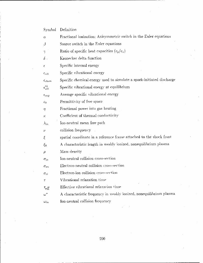
Symbol Definition

a Fractional ionization; Axisymmetric switch in the Euler equations

ß Source switch in the Euler equations

7 Ratio of specific heat capacities (cp/cv)

S Kronecker delta function

e Specific internal energy

evib Specific vibrational energy

echem Specific chemical energy used to simulate a spark-initiated discharge

eeLq

ih Specific vibrational energy at equilibrium

taVg Average specific vibrational energy

e0 Permittivity of free space

j] Fractional power into gas heating

K Coefficient of thermal conductivity

\in Ion-neutral mean free path

v collision frequency

£ spatial coordinate in a reference frame attached to the shock front

£0 A characteristic length in weakly ionized, nonequilibrium plasma

p Mass density

(Tin Ion-neutral collision cross-section

aen Electron-neutral collision cross-section

crei Electron-ion collision cross-section

T Vibrational relaxation time

reg- Effective vibrational relaxation time

u;* A characteristic frequency in weakly ionized, nonequilibrium plasma

ujin Ion-neutral collision frequency

200

Appendix B. Two-Dimensional Fluid Dynamics Code Description

B. 1 Introduction

The influence of thermal inhomogeneities on the propagation of shocks was

studied with the use of a computational fluid dynamics code. This code solves

the two-dimensional Euler equations using the explicit MacCormack scheme [82].

A flux corrected transport (FCT) algorithm [23] is used in conjunction with the

MacCormack scheme to reduce numerical oscillations that occur in regions of sharp

gradients, such as around shocks. Strang-type splitting operators [109] are used in

order to solve the differential equations in two spatial dimensions. This method is

commonly used in order to extend a one-dimensional method to higher dimensions.

The MacCormack scheme (with second-order accuracy) was chosen due to both

its suitability for solving nonlinear Equations [62:192] and its relative programming

ease. However, the use of a second-order accurate method by itself would lead to

oscillations in the solution near shocks. The FCT method was adopted as a way

to get rid of these numerical oscillations by preventing them before they are al-

lowed to grow [61:127]. Of course, other methods could be used to accomplish the

same goal (Godunov method [47], artificial viscosity, etc.), however the MacCor-

mack/FCT method offers stability and sharp resolution for a relatively small effort

in coding [112]. Higher-order Gondunov schemes like the Roe method [99] produce

more accurate solutions than the MacCormack/FCT scheme, however they are more

complicated to code and more expensive to run [44:173]. Additionally, the FCT

method is more accurate than using artificial viscosity to clamp out the oscillations

[44:173].

B.2 Nondimensionalization of Equations

The Euler equations describe the flow of an inviscid, compressible fluid. They

are given in a compact form in Equation 95 for two-dimensional axisymmetric (o = 1)

201

or planar (a = 0) geometries, where the vectors U,E,F,H and Q were defined in

Chapter V by Equations 83 through 87. The vectors on the left hand side of Equation

95 are the conserved variables (£■'") and the numerical fluxes {E and F). The vectors

on the right hand side are sources clue to axisymmetry (H) and energy addition (Q).

This latter source vector allows for the treatment of spark-initiated shocks (if ß = 1).

dU 8E OF T-t - /nr.

at ox ay

These equations are nondimensionalized so that the values of the variables will be

of order 1, making it convenient to analyze the results. Additionally, nondimension-

alization reduces the possibility of either an underflow or overflow error.

The parameters used to nondimensionalize the variables appearing in Equation

95 are the ambient density (p0), the ambient temperature (T0), the thermal velocity

at the ambient temperature (Vth = \TM ) and the lenStn of tne snock tube (L0).

Using these parameters, the nondimensional variables can be defined as

(96)

where the nondimensional variables are denoted with a prime.

B.3 Model Equations (nondimensional)

Using the nondimensional variables defined in above, the dimensional Euler

equations (Equation 95) can be transformed into a nondimensional system of equa-

tions: ?* + °* + aPL = _agl + ßQ (97) at' ox' ay'

*'=£. v' = JL y L0' *' = '&

p'=^ rpl T 1 - T0'

J — f-chf.m ^chem — V\

th

v* vth' V = ^ y Vth

202

with V defined as

U' =

p'

PX

PX

s{i{w 2 + v?) + ^'}

rt'f'

(981

where p' is the nondimensional mass density of the gas, V^ is the nondimensional flow

velocity in the x direction, Vy' is the nondimensional flow velocity in the y direction,

7 is the usual ratio of specific heats, V is the nondimensional gas temperature and

e'chem is the nondimensional specific chemical energy to be used in generating a shock

in the spark-discharge case. Each of the variables in U' is a function of x\ y' and t';

i.e., p' = p'{x',y'J'), V; = V^{x',y'J'), etc. The flux vectors E' and F' are defined

as

PX

P'(V? + T')

and

E' PXK

n'f' V r ^chem y x

(99)

F' =

PX

P'V^y

P> (v- + r)

n'f' V

(100)

203

the axisymmetric source vector H' is defined as

H> = - PV

n'e' V I ^chem ' y

ior

while the vector of sources used for the spark-initiated shock problem is defined as

Q' =

p'f\

p'f-\ y chem

:io2)

where r' governs the temporal release of the chemical energy. The first equation in

97 expresses conservation of mass, the second and third equations describe the con-

servation of momentum in the x and y directions, respectively. The fourth equation

expresses the conservation of directed kinetic energy and thermal energy, and the

fifth equation expresses the conservation of chemical energy.

Note that in the axisymmetric source vector (Equation 101) there appears to be

the possibility of a singularity when y' is zero (along the centerline). By application

of L'Hospital's rule to each element of the array, it can be shown that this is not the

case. While the use of symmetry arguments requiring such terms as f^, ^f, etc. to

be zero are necessary to accomplish this, such arguments are entirely justifiable in

the axisymmetric geometry.

Equation 97 can be modified to include viscosity and/or thermal conductivity

if desired. The modifications necessary to include these processes in the present code

204

are straightforward, although the construction of the analytic Jacobian matrices used

in the solution method can be tedious.

B.-{ Strang-Splitting Operators

The temporal and spatial integration of the two-dimensional Euler equations

can be written as a series of one-dimensional operations acting on the solution

[120:122]. The general formulation can be written as

U'n+2 = Lf 'I2 Lf L?f Lf Lf If if7'2 U'n (103)

where time is indexed by n. The vector of conserved variables at time tn is denoted -* 71 + 2

by U'n (Equation 98). The solution two time steps later is denoted by U' . The

operators L^' and Lf*' represent the temporal integration (over a time period of

At') and the one-dimensional spatial integration of the homogeneous fluid equations

containing the x' and y' derivatives, respectively. The operator Lf* represents the

temporal integration (over a time period of At') of the fluid equations assuming

the flow to be frozen (i.e., during this integration the fluid is not converted). The

symmetric sequence of operations given in Equation 103 is necessary in order to

maintain the second order accuracy contained in the individual operations themselves

[61]. Each of the operators will be described in detail in the sections to follow.

Yee [120:38] points out that such a method has advantages in that good algo-

rithms already exist that can handle each part of the problem well. In other words,

good numerical techniques already exist that integrate the homogeneous fluid equa-

tions and other good techniques exist which can integrate the ordinary differential

equations describing the source terms. Using an operator methodology is a quick

and simple way to combine the two types of problems with a reasonable hope for

success, and may even give better results than an algorithm which attempts to solve

both types of problems at once.

205

In practice, Equation 103 was split into two series of operations, with the

decision of which one to use determined by whether the time step n was odd or even:

V n+l

u- n+l

Ltt>/2 Ltf L$* Lf2 U'n for n odd

L?'2 Lf L$' Lf'2 it" for n even

(104)

(105)

This was done in order to have access to the solution after each time step, instead

of after every other time step. This may not be necessary, but in the original for-

mulation of the solution method it was thought that some parameters should be

as highly resolved in time as possible (e.g., shock position, integrated density and

PADS signal).

U""= Solution at time n+1

Ly Sweep

At' x' Figure 100. Application of Strang-type operators showing sequential sweeps of L

and Ly/' through the computational domain. L^f is first applied hor-

izontally to each j line, then Lf,1' is applied vertically to each i line

(adapted from [62:131]).

206

An illustration of the application of Strang-type operators is shown in Figure

100. Here, Equation 105 (specialized for the case in which no sources are present)

is applied to a known solution. The L*/' operator is applied to the known solution

first. A sweep of L^f is made down each j line throughout the domain. Then the

LY operator is applied to the intermediate solution, sweeping Lpf up each ■/ line

throughout the domain. On the next time cycle, the order of the x and y sweeps

will be interchanged.

B.4.I x Sweep Operator. The L**' operator solves the equation

f + ^ = 0 (106, at' ax'

using an algorithm given by Fletcher [44:153-173]. This algorithm combines a second-

order accurate MacCormack scheme with a flux corrected transport scheme. In

the notation that follows, primes will be dropped from the variables, with noncli-

mensional quantities implicitly assumed. Cell interfaces are located at a*;+i/2.j and

Zi-i/2.j, with a-i+i/2,j = (Xi,j +';r,-+i.j)/2. The subscript i + 1/2 refers to a quan-

tity centered on the cell interface at £i+1/2,j. The difference of conserved variables

in adjacent cells is given by AUi+i/2,j = Ui+\,3 - Lh,j- Both steps of the MacCor-

mack predictor-corrector method are first accomplished before applying the FCT

algorithm:

% = ^- + ^)-^A--^w) (108)

where a forward difference is used in the predictor (Equation 107) and a backward

difference is used in the corrector (Equation 108). This is consistent with the general

usage of the MacCormack method in which the flux E is differenced in the direction

of shock propagation in the predictor, and in the opposite direction in the corrector;

20<

i.e., in the problems investigated using this algorithm the shock always propagated

in the positive x direction, which was the direction in which the i index increased. In

Equations 107 and 108 the superscripts t and T refer to the time at the half step and

full step, respectively. Note that the calculation of El requires the half-step solution

Uf be decoded in order to determine the primitive variables, then constructed using

Equation 99.

The trademark of the FCT method is the use of diffusive and anti-diffusive

fluxes. The former is used to add numerical diffusion to the solution in order to

ensure stability and monotonicity, while the latter is used to eliminate the excessive

numerical diffusion where possible [112:84]. Following the predictor and corrector

steps, the FCT algorithm is applied to the solution in the following format:

Ufj = Ul + DV±1/2J - Dll/2J (109)

u-Jl = %-^lh + ^lh (no)

where the superscript d denotes the diffused solution and D and A are the diffusive

and corrected anti-diffusive fluxes, respectively.

The diffusive flux is defined as

flr+i/w = *r+i/2jAf?+1/2j- an)

where v is defined as

with e given by

and AUn is given by

1 1 U?+l/2J = g + 3(e!-+i/2.j)

A , /yn , yn '

'l+l^ ~ Ax { 2

'112)

113)

Af^i/2,^^-^- (114)

208

The value of the anti-diffusive flux is controlled by a limiter, with the intent to

prevent the appearance of new maxima or minima in the solution [112:85]. The flux

limiter is the key to the FCT method, as it "effectively allows the diffusion introduced

in the predictor stage to selectively annihilate the dispersive 'ripples"' generated

by the second-order accurate MacCormack algorithm [44:165]. The corrected (or

limited) anti-diffusive flux is defined as

Tn+l/2 n+1/2 n • /u°+1'2 | n+1/2 A ffd "+1/2 xf}d

where AUd is given by

The uncorrected anti-diffusive flux A is defined as

r+/2 _ „n+1/2 Atfi Ai+1/2J ~ /-li+l/2.jlAVi+l/2,

with // defined as

,,n — _ _ -(tn \ t-li+l/2,j - g glS+l/2,ji

115)

Wi+i,2j = vf+1J-ü!j, die)

sn+l/2 js clef|necl as

*£& = ^«(4-+i/2J-). (117

"n+/2 ?+V».AC7?\,,.. (118)

;ii9)

and with e given by Equation 113. The term AUT is given by

■ ^l^ = Ulu-Ul, (120)

The description of the L^' operator is now complete.

B.4.2 y Sweep Operator. The Lf*' operator solves the equation

8Ü' dF'

209

using a MacCormack predictor-corrector scheme in combination with a flux corrected

transport algorithm, as reported by Toth [112]. This method is different than the

algorithm represented by the Lf,f' operator discussed previously. It was found that

the algorithm presented here for Lpf' gave better results along the centerline and

wall of the shock tube than Fletcher's algorithm. Specifically, it was found that

the value of Vy' in these locations was not zero (or very close to zero, as compared

to values of V' in adjacent bins) when the L^' operator discussed previously was

adapted to the y direction. With the use of the algorithm reported by Toth however,

V' was zero (or very close to zero) for all points along the centerline and wall. More

on this subject can be found in the section on boundary conditions, contained in this

appendix.

Consistent with Toth's method, the flux vector F' (Equation 100) is rearranged

slightly, putting Equation 121 in strict conservation law form. Equation 121 is thus

transformed into ^ t

^ + ^L = S' (122) at' dy' ~

where U' remains unchanged, F[ is given by

F{ =

p'K W'„ P'V?

M{k{v? + \\ri) + +TT>}

P'<'., K

;i23)

210

and the new source vector S' is given by

j9_

dy'

0

0

-p'V

-ptT'Vl

0

;i24)

In the notation that follows, primes will be dropped with nondimensional quan-

tities implicitly assumed. Cell interfaces are located at l/ij-1/2 and t/j.j+1/2, with

yij+1/2 - (Vi.j + J/i,j+i)/2- The subscript j + 1/2 will refer to a quantity centered on

the cell interface at y;,;+i/2- The difference of conserved variables in adjacent cells is

given by AUt,j+i/2 = Ihj+i - Utj.

Toth's algorithm advances the solution from time n to time n + 1 in two steps:

a half step and a full step:

The half step:

u< 1,3

fld.

frn+1/2

Ui,j + A\j+l/2 - A"i-l/2

Ui,j ~ Atj+l/2 + A,j-l/2

;i25)

;i26)

:i27)

The full step:

U1-

U, D i-3

Unfl

Un- Ai pn+l/2 rh+l/2 , , A , r?n+l/2

Ui.j + 1/2 ~ JiJ-1/2) + ^"ij Ay

Ui,3 + Ui,j+l/2

ÜZ -A.

D n+1/2

hj

fn+l/2 Tn+l/2

ij-l/2

1+1/2 i.j-1/2

128)

129)

130)

211

where D and .4 refer to the diffusive flux and corrected anti-diffusive flux, respec-

tively, which are trademarks of the FCT method. The flux / used in Equations 125

and 128 is given by

Ji,j + l/2 - L iJ+1/2 Vj + l/2

A+l/2 rn+l/2 fi,j+l/2 - W,j+l/2vyt,J+1/

'131'

where U?J+1/2 = (UW + Uij)/2 and VyiJ+l/2 = (Vy„J+l + VViJ)/2. Note that Un

is used to compute the flux at time n + 1/2. The use of fluxes centered at the

cell interfaces in Equations 125 and 128 ensures the conservation property of the

Equations [112:84]. The source terms S appearing in Equations 125 and 128, are

second-order finite-differenced representations of those defined in equation 124.

The diffusive and anti-diffusive fluxes are defined in a manner analogous to

those given for the L^f operator. The diffusive fluxes are defined as

A"j+i/2 - ^+l/2Af/^+l /2

ftn+1/2 _ n+1/2 xfjn :i32)

where Un is used in computing the diffusion flux at time n + 1/2.

The value of the anti-diffusive flux is controlled by a limiter. with the intent

to prevent the appearance of new maxima or minima in the solution [112:85]. This

flux, called the corrected anti-diffusive flux, is defined as

An — an

^i,j+l/2 — bi,j+l/2 max 0, min{ |AiJ+1/2|, s^+1/2Acrij_1/2, slJ+l/2AUiJ+3/2

^+1/2 n+l/2 iJ+1/2'

tn+l/2 n • l\ 1 I "+1/2 \T~JD n+1/2 ,\fjD 0, min{\Ait j+1/2|, stJ+l/2AVitJ_l/2, t>iJ+1/2^ViJ+3/2 :i33)

212

where $?j+1/2 = sgn(±Ü?J+1/2) and <j"+{/2 = sgn(AlfJ+l/2). The term iiij+/2 is

labeled the uncorrected anti-diffusive flux and is defined as

-*n _, Ai,j+/2 = ^lj + l/2^Ui.j+l/2

The terms v and \x appearing in equations 132 and 134 are defined as

,,n _ ! , !/,ra x2 ,.1+1/2 _ I , If "+1/2 y2 ^i.j+1/2 - g + 2lS,j+l/2i ' Ui.j+l/2 - 6 ^ 3 ^,, + 1/2^

„n -1 ^^ -|2 .«+1/2 _ 1 _ I|Vn+l/2 V2 (ion /*«,j+l/2 - g _ glfc

i,j + l/2i - /Xi.j+l/2 - 6 6^^+1/2 J l1'3'^

W here 1 At. .„ „4.1 /o At vn fn+1/2 - _T/n+1/2 mfn

S,j+i/2 - 2^^+1/2< fcij+i/2 ^lwJ+i/2' {lou>

With these definitions the formulation of the Lp1' operator is complete.

B.4.3 Source Operator. The L^'l2 operator solves the equation

dÜ' dv aH' + ßQ' (13/

using an implicit method suggested by Yee [120:38]. First, however, remember that

Q' describes the energy density per unit time that is either lost or gained by the fluid

during the detonation process for a spark-initiated shock. For a Riemann shock, this

term will be zero. The axisymmetric source terms are contained in H', which will

be nonzero only in the axisymmetric geometry. Therefore, the Lf*'/'2 operator will

need to be used only if a spark-initiated shock problem is to be solved and/or the

geometry is axisymmetric. To start, rewrite Equation 137 using finite-difference

notation in which a half-time step is used on the left hand side and the right hand

213

side is represented by an average of the sources at each time:

U'n+> - U'n = Q'(Ü>n) + Q(rn+t) + H'(U'n) + H>(ü>n+") {m)

Af/2 9

This can be rewritten as

I -n+k

-U' 4

;n+2 H'(U> ) + H'(U> 2) + Q'(U' ) + Q'(U> jn+i

;i39)

r-tn+i The terms H'{U'n 2) and Q'iÜ1'^2) are functions of the conserved variables at the

1/2 time step and are thus unknown. In order to solve the equation, these terms are

linearized, using

H>(U'n+2 H'(U> ) + dW dÜ'

[U^-U^ 140)

and

Q'(U'nH Q'(U' ) + -» n V 141'

In these equations, the terms (j^j and f |^J are 5x5 Jacobian matrices, to be

evaluated at time step n. These Jacobians are of the usual form, i.e.

dU'

dU[

dQ'2

dU[

dQ's BU[

dQ'4

dU[

dQ'5

8Q\

dQ'2

dV2

dQ'z du'2

dQ'4

m du'

9Q\

dQ'2

din dQ'z

mi dQ'

aui dQ'2

di''4

dQ'A

■dU{

dQ'

£9i

dU's

din

dQ'4

dQ' dm am dui

142)

214

Carrying out the operations required in Equation 142 results in

and

w here

dcr_ du1

oooo o

0 0 0 0 0

0 0 0 0 0

0 0 0 0 £

0. 0 0 o -h

dw_ i_

y7

0 0 1 0 0

-V'V x y v; v; 0 0

-V'2

V 0 W 0 0

Mi -442 A43 TV; 0

-e'u V 0 cc7iem 0 K

'143)

144)

Mi

A42

A43

V' h-W? + K)-*>*

= iet .7-1

, )W + My '2\

(145)

(146)

(147)

with e't = \{V? + Vy'2) + -^zjT'. The derivations of these Jacobians are straightfor-

ward, but can be tedious. Note, again, the apparent possibility of a singularity in

Equation 144 along the centerline (y' = 0) in the axisvmmetric geometry. However,

it must be remembered that the axisymmetrir sources are zero along the centerline,

therefore the use of this Jacobian is limited to points away from the centerline.

Combining Equations 140 and 141 with Equation 139 results in

«• At' -» \ n

dH'

dU' +

dÜ1 Ab •,"+2 At' ,~..^n

9 H>{Ü>n) + Q>{Ü'n)) (148)

215

w here

Ml'n+h- = U'n+h - U'n (149)

and J is the 5x5 identity matrix. Equation 148 is the chief result of this section

and is the equation to which the Lf *'/2 operator is applied. With the solution U'

known at time step n, all terms in equation 148 are known except AW ". putting

this equation in the familiar form A X = B (where A and B are known). Equation •n+}-

148 is solved for AU' 2 at each interior grid node at every time step, using an LU

decomposition method with back

be found by use of Equation 149.

decomposition method with back substitution. Once AU' 2 is known, U' 2 can

B.5 Initial Conditions

The initial conditions used in the code depend on the type of problem to be

solved (Riemann or spark-initiated). In general, however, the initial values of the

primitive variables (p,T,Vr,Vy,echem) are defined in two stages. The first stage de-

fines the values of the variables for the nominal case, while the second stage modifies

the density and temperature to account for a heated region in the flow.

In the Riemann problem, the first stage amounts to specifying the values of the

variables on both sides of the diaphragm. In this case, all velocities and the chemical

energy at each grid node are specified to be zero, and the density and temperature

on the low and higher pressure sides of the shock tube are set equal to the values

determined from the input conditions. In the spark-initiated shock problem, the first

stage sets the density and temperature at each grid node to their ambient values,

and all velocities are set to zero. The chemical energy at each grid node throughout

the domain is set to zero, except for the grid points along the left edge of the shock

tube. These are set equal to the value determined from the input conditions. The

chemical energy along this edge of the shock tube simulates the explosive release of

energy from a spark discharge and leads to the development of a shock.

216

If no changes were made to these input conditions the computer would solve the

typical Riemann problem or generate and propagate a spark-initiated shock through

a homogeneous gas. To account for a heated region in the flow, the temperature is

adjusted at each grid point to the desired level. Since the pressure is assumed to be

a constant throughout the heated region, the density must also be adjusted by the

appropriate amount at each nodal point.

B.6 Boundary Conditions

Application of the correct boundary conditions is an important part of the

solution method used in the code. The boundary conditions applied to the model

equations are

along the wall (y = 0) and centerline (y = ywaii):

dy u dy dy V dy (150)

along the left (x = xiejt) and right ends (x = xright)-

^ = o ^ = o v; = o ^ = 0 %^ = o dx ox x Ox ox

where y is the transverse coordinate in the f or y direction, depending on whether

the geometry is axisymmetric or planar, respectively.

Since the solution to the problem is assumed to be independent of either the 0

(in the cylindrical case) or z (in the planar case) coordinate we can take advantage

of the symmetry and solve only half of the problem. The physical layout of the shock

tube (shown in Figure 101) illustrates how the geometry of the problem is represented

within the computer. The shock tube's centerline, wall and left and right ends are

shown. The x and y coordinates are indexed by i and j, respectively. The physical

boundaries of the shock tube within the grid are i = 2 (left edge), i = IL - 1 (right

edge), j = 2 (centerline) and j = JL-l (wall). Notice that the physical boundaries

of the shock tube do not lie at the edge of the computational boundaries. A row of

'ghost' nodes lies beyond the centerline and wall of the shock tube, while a column

217

of 'ghost' nodes lies to the left of the left edge of the tube and to the right of the

right edge of the tube. The use of ghost nodes at the boundaries was necessary in

order to incorporate the reflection boundary conditions [3:284], which are used in

the code. The flow parameters are defined at the grid nodes (indicated by the dots

at the intersections of the i and j lines) in the finite-difference form of the governing

equations.

computational domain ghost nodes

(UL) wall

left end

• • ,...*.

■<►■■#■

rh ♦—•

-/■

■#—#

(IL.JL) j=JL

• j=JL-l

# j=JL-2

right end

♦ ■••♦•/• ■#•••♦ •!■#■••#■••

ghost nodes' centerline

physical domain

i=IL-l i=IL

j=3

j=2

=11 ^ (IL,1)

Figure 101. Representation of the shock tube geometry used in the code.

When applied to the grid shown in Figure 101, the boundary conditions spec-

ified by Equation 150 become

218

Along tube wall: (i=2, IL-1)

Ti.JL = Ti.jL-2 VVi JL = -Vyt JL_2

Along tube centerline: (i=2, IL-1)

P(,l = Pi,3 Kru = r'xi.3 £chemtA = ^chem,*

Ti^i = Ti,3 \'ytl — —Vyti3

Along left end: (j = l, IL)

PlJ = P3,j •'i'lj = — *'^3,j ec/iemi,_, = (-chemtj

Tlj = r3J Vyi ^ = Vyjj

Along right end: (j=l, IL)

PlL,j = PlL-2,3 V'XIL.J = ~*XIL-2,J

echemILtJ — (-chemIL_2,3

TIL,J = TIL-2,j VyjLi> = Vy/L_2;

These boundary conditions were applied to the solution each time a Strang-

type operator {L^\ Zy'\ L^f'/2) was used, as well as at different points within the

algorithm represented by each operator.

B.7 Determination of Time Step

In explicit integration schemes the time step is limited by the Courant-Friedrichs-

Levy (CFL) criteria, which in one-dimensional takes the form (assuming a constant

grid spacing of Ax): (CFL)Ax ,iri '

At < — 151 — t\\' \ M rf \ \ I y x I i *~'s I max

where CFL is a number less than unity and Cs is the sound speed. Transforming this

equation to the nondimensional form required by the code and taking into account

both the discrete nature of the grid and the dimensional splitting of the integration

219

results in

,*,,, < „,,■„,, J^fl. (Aa<m,nij(^L (1,2) U V:r;,j I "+" L's,:.j ^ vl v

yi.j I 1" ^ s;,^

where C's = y/jT'.

Consistent with the algorithms represented by the L^' and Lpf' operators, a

CFL number of 0.4 was used [44:166], [112:85], resulting in a global time step At'

determined by

At' = 0.4 [{&t')x, (At')u]min (153)

The time step given by Equation 153 was determined based only on the CFL

criteria. The computation of flows in which physical processes like energy transfer

occur may require one to take into account the time scale of the process. In the

spark-initiated shock problem the variable r' determines the time scale associated

with the energy release used to generate the shock. Taking into account this time

scale, the calculation time step should be modified to be

At'<{{At')cFLAr')\min. (154)

In practice, r' was hardwired to be equal to 20 to 100 times the value of At\ thus

At1 was always determined by the CFL limit.

B.8 Code Flowchart

A brief flowchart of the main features of the code is shown in Figure 102.

The input file defines the problem to be solved, specifying whether the Riemann-

type problem or the spark-initiated shock problem is to be run. It also defines the

geometry (two-dimensional planar or axisymmetric). physical size of the shock tube

(length and width), type of gas, as well as the ambient pressure and temperature.

In addition, the size of the computational grid to be used is also specified. Finally,

220

Propagate Solution fn odd: equation (104)1 n even: equatk>n(105)]

Write Intermediate Data to Files

Met Stopping Criteria? No

Yes

Write Out Final Solution

| Stop |

Figure 102. Two-dimensional fluid dynamics code flowchart.

the input file determines whether the problem is to be run from scratch or initiated

from a restart file. If a restart file is not used, the code generates the geometric grid

and initializes all variables according to the input parameters. If a restart is used,

these actions are accomplished by reading in the appropriate values from a previous

simulation.

After the computational time step is determined (using Equation 154), the

solution at a known point in time is propagated according to either equation 104 or

105, depending on whether the value of the iteration counter is odd or even. After

each time step, some data is written to external files for post-processing and/or flow

visualization. If the stopping criteria is not met, the code increments the iteration

221

counter and loops back to establish a new computational time step, propagates the

solution to a new time, writes intermediate data, and then rechecks the stopping

criteria. The stopping criteria is based on one of three different conditions and

is determined by the input file. The code can either run for a certain number, of

iterations, or until a certain physical time is reached, or until the shock front along

the centerline reaches a particular location. These choices allow the user to select

the type of stopping criteria, most useful for the particular problem at hand. In any

case, if the stopping criteria is met the code exits the propagation loop, writes out

the final solution and stops.

B.9 Determination of Shock Velocity

Although not calculated directly by the code, the determination of the shock

velocity is such an important parameter in the analysis of shock propagation that

a, description of its calculation is warranted. While the code determines Vr and Vy,

these are average fluid velocities, not shock velocities. The determination of the

shock velocity is determined by an analysis of the position of the shock front as a

function of time.

After each time step, the location of the shock front along the centerline of the

shock tube is determined. This is accomplished by finding the first spatial bin in

which the nondimensional pressure, which is always initialized to unity, has a value

greater than 1.01. The search for this particular bin always starts from the right

end of the shock tube and proceeds to the left, which is the direction opposite of

the shock velocity. The value of 1.01 was found to be a good compromise between a

lower number (which would be subject to small numerical oscillations in front of the

shock and could place the computed shock front location slightly to the right of the

actual shock front location) and a larger number (which would place the computed

shock front location slightly to the left of the actual shock front location). Once

this bin was found, the x position corresponding to it and the time corresponding to

000

the calculation were written to an external file. The process of searching for the bin

containing the shock front was accomplished every time step. The data was written

to the external file only if the location of the shock front changed between consecutive

time steps. Thus, as the program runs, a temporal history is built describing the

location of the shock front. This file is post-processed to determine the shock velocity

by computing the slope of the position vs time curve (Vshock = j[)-

Care must be exercised in the calculation of this slope as the effects of a fi-

nite sized grid lead to some noise in the data. Through considerable effort a sat-

isfactorily method was found that was quite accurate in validation tests against

analytic (Riemann) solutions. The method consists of finding the slope of a line

defined by a linear least squares fit to a group of data points centered around the

time level of interest. For example, say that the shock velocity at a time level of

n (corresponding to a physical time of tn) is to be computed. From the exter-

nal data file, the values of the shock positions at ten data points before through

ten data points after the interested time level are extracted. These x locations

are labeled as xn_io, £n_9, xn-8 ...xn... .r„+8, xn+9l .r„+io, where the shock position

at time tn is xn. The times corresponding to these shock locations are labeled as

f n_io, f„_9, tn-s ...tn--- tn+8ltn+9, tn+l0. With these ordered pairs of data, a linear-

least squares fitting routine is used to draw a line through these points, from which

the slope can be determined, which defines the shock velocity at time tn. The shock

velocities at times in+i,tn+2, etc. are determined similarly. Notice that shock veloc-

ities cannot be determined for times that correspond to either the first or last ten

data points within the data set. In practice, this is a small restriction and is of little

consequence.

223

Appendix C. Two-Fluid Plasma Code Description

This appendix offers a short description of the plasma fluid code used in the

time-dependent calculations of Chapter III. The code, based on the MacCormack

method with flux corrected transport (FCT) as given by Toth, et al. [112], solves

the one-dimensional equations for a plasma in the two fluid approximation. The

assumptions upon which the two fluid approximation is based have already been

given in Chapter III and will not be repeated here.

The two fluid plasma equations (given by Equations 52 to 62) were nondimen-

sionalized so that the value of all variables was of the order of one. The density

and temperature of each component were nondimensionalized with. respect to the

respective upstream ambient values. For example, the ion density was normalized

with respect to the upstream ambient ion density, while the neutral density was

normalized with respect to the upstream ambient neutral density. Thus, although

the fractional ionization of the plasma may be very low (10~6, for example), the

computed density of both fluid components will be of order one. The flow velocities

of each component were normalized with respect to the upstream ambient thermal

velocity. Since the ions and neutrals were assumed to be in thermal equilibrium in

the upstream ambient conditions, the thermal velocity was the same in both cases.

The inputs to the code are divided into computational parameters and physical

parameters. The physical parameters are

• To - ambient heavy particle temperature (K)

• P0 - ambient heavy particle pressure (torr)

• 7 - heavy particle specific heat ratio (unitless)

• Te - electron temperature (K)

• a - fractional ionization (unitless)

224

• ain - ion/neutral collision cross-section (m2)

• aen - electron/neutral collision cross-section (m2)

• aei - electron/ion collision cross-section (m2)

• L - physical length of the shock tube (m)

• -P4/P1 - ratio of the high pressure to the low pressure for the shock tube

• T4/T1 - ratio of the heavy particle temperature in the high pressure side to the

heavy particle temperature in the low pressure side

• ;rdia " l°ca-tioii of the diaphragm (m)

These parameters are all self-explanatory. In all the calculations performed, aen and

aei were set to zero. Thus, only ion-neutral interactions were allowed to play a role

in the shock dynamics. Since a Riemann problem was used to generate the shock,

the parameters F4/P1 and T4/T1 determined the neutral shock speed for a given 7

(in the absence of ion/neutral interactions), while the computational parameters are

• NX - number of bins

• stopping criteria

• restart (Y/N)

• computer system (PC/UNIX)

The stopping criteria determined when the calculation would end, and could be

defined in one of three ways. The total number of time steps for the calculation

could be specified, or the time (in seconds) at which the calculation should end

could be specified or the final position of the shock front could be specified. The

restart capability allows the program to pick up the calculation at a previous point.

Once the inputs to the code were read in. all variables were initialized and the

code entered the main program loop. Here, the following steps were performed each

time iteration:

225

• calculate the time step

• calculate the source terms

• propagate the solution one time step

The time step was determined based on-the usual Courant-Friedrichs-Lewy

(CFL) criteria used in explicit computational fluid dynamics codes [3:76]. For the

neutral fluid, this amounts to

(CFL)Az ,1rp, (**)n < ,r\ ■ y h , (155)

l<- n+ I Vn | jmax

where Cn is the neutral sound speed and Vn is the neutral flow speed. The CFL num-

ber is determined by the numerical algorithm. For the present choice of algorithms,

Toth [112] recommends CFL < 0.5. In all calculations using the present code, CFL

was equal to 0.4. Whereas the sound speed (Cn) was used in determining At in the

neutral component, the ion-acoustic sound speed (Ci0) is used in determining At in

the plasma component. Thus, the time step for the plasma component is

(CFL)AJ ,ir_, (At), < \ ; • (156)

[t'ia+ \ vi |)max

When transformed to a computational grid, these become

m„<^Jß^-, (AOj<™J?J<fl£- (157)

where j indexes the spatial grid. The time step for the calculation was determined

by choosing the smallest time step meeting both criteria above. Thus,

At = [(A*)n, (At),-]min (158)

determines the computational time step for both components.

226

The source terms were calculated by use of Equations 55 through 62. These

source terms are divided into three types. Some source terms are a result of the form

of the Euler equations used in the calculation and are not connected with the plasma,

in any way (Equation 55). Some source terms are due to the ion/neutral collisions

(Equation 56), while others are a result of the presence of an electric field (Equation

62). Note that the last of these source terms affects only the ion fluid, as required.

With the time step and source terms determined, the solution is propagated

one time step using the algorithm reported by Toth [112], and previously reported in

Appendix B as the Lf* operator. A detailed description of this operator was given

there and will not be repeated here. However, a brief comment on the application

of the FCT will be made. Since there are two flow velocities in the plasma code, the

FCT scheme must be applied to each fluid separately, based on the flow velocity of

the appropriate component.

In practice, extensive use of the restart capability of the code was required.

Transients in the flow parameters near the diaphragm were observed at very early

times. With large values of the electron temperature and ion/neutral interaction

cross-section, these transients became very large and forced the calculation to end

prematurely clue to numerical oscillations. Allowing the shock to form and begin to

propagate away from the diaphragm before turning on the source terms clue to the

ion/neutral interaction and the electric field eliminated this problem.

227

Appendix D. Self-Consistent Model of Gas Heating in a Glow

Discharge

One of the difficulties in assessing the influence of thermal effects on shock

propagation in a plasma is the determination of the gas temperature at each point

in the shock tube. This is particularly true when experimental data, of various shock

wave parameters (density, pressure, velocity, etc) are reported, with no accompanying

gas temperature data. In the absence of such thermal data, the temperature profiles

must be calculated. In the general case, the time dependent energy equation should

be solved, which requires the simultaneous solution of a coupled set of equations

(conservation of mass, momentum and energy) in addition to a detailed knowledge

of the form of the heat source term. This level of detail is generally lacking in the

case of transient gas discharges. However, in the case of steady-state gas discharges

the problem is simplified considerably, and, generally speaking, enough experimental

data is available for a calculation to be carried out.

D.l Problem Statement

The steady-state heat conduction equation for a neutral gas heated by a gas

discharge is

V-(KVT) = -»7 (J-E) (159)

where K is the thermal conductivity (and is a function of temperature), T is the

neutral gas temperature, J is the current density and E is the electric field. The

objective is to solve this equation for the neutral gas temperature (as a function of

radial position) given the experimentally determined values of the electric field and

total current in the discharge. The difficulty lies in the treatment of the source term,

which is itself a function of the temperature. This difficulty will be addressed in the

next section. J • E represents the total power input to the electrons from the external

circuit. Some of this power is used to ionize the neutral gas to sustain the discharge,

228

some is used to excite bound electrons into higher energy states (thereby producing

radiation) and some is used to heat the gas through electron-neutral. The fraction

of the total power that goes into gas heating (?;), is a function of the EjN ratio

(ratio of the electric field to neutral number density) in the positive column of a gas

discharge. For rare gases, 77 can be considered to be the fraction of the power that

goes into momentum transfer collisions [66]. For molecular gases, 17 can be estimated

as the fraction of the total power that does not go into either ionization or electronic

excitation.

Anticipating the cylindrical geometry of the experimental arrangement, Equa-

tion 159 is cast in cylindrical coordinates, resulting in

cPT = _\_dT_ _ Qjj± _ l^ck fdT\2 (160)

dr2 r dr K K dT \dr)

where Q[r) = >][J ■ E\. Note that the possibility of a singularity exists in the first

term on the right hand side. By application of L'HospitaFs rule and by assuming

cylindrical symmetry, this term limits to -^ at small r. Therefore, two forms of

Equation 160 result, one valid for points very near the origin and the other valid for

points further removed from the origin:

d2T 1 Q{r) ld/c/tfT K K dT \dr / dr2 2

d2T ldT Q{r) Idn (dT'

dr2 r dr K K dT \ dr

for r % 0 (161]

for r 9^0 (162)

Computationally, Equation 161 is solved at the origin, while Equation 162 is solved at

every other point in the r domain. A standard Runga-Kutta fourth order technique

is used to integrate the differential equation in space.

229

D.2 Source Term

As mentioned previously, the difficulty in solving Equation 159 lies in the source

term. For a given temperature profile (T(r)) the source term is known, however T(r)

is not known a priori. Therefore an iterative computational scheme is used in which

an initial T[r) profile is assumed. Using this initial (or guess) T{r) profile to define

the source term, Equation 160 is solved for a new T(r) profile. This new T(r)

profile is then used to define a new source term, and the process is repeated until

convergence is achieved. Therefore, although the final temperature profile is not

known in the beginning, the functional form of the source term for a given T(r) is

known, and is used to determine the steady-state solution in a self-consistent manner

which conserves the total current in the discharge. The source term Q(r) is defined

as

Q(r) = ri(E/N)[J(r)-E] (163)

where r) (the fraction of the total power that goes into gas heating) has been written

explicitly as a function of the E/N ratio and the current density (J) is a function of

position.

The current density in the positive column (where the electrons are the ma-

jority charge carrier) can be defined as

J(r) = ne(r)qf- ^</<(^7j) (164)

where ne is the number density of electrons. </, is t he charge on an electron and I'dri/t

is the drift velocity of the electron in the applied E field. Vdrift is a function only of

E/N within the positive column of the discharge for a given gas (Figure 106). E/N

is a function of the electric field, (which is assumed to be constant over the discharge

tube radius [83]) and the neutral number density, which is a function of pressure and

230

temperature given the equation of state P = NkBT. Thus,

§(r) = jkBT(r) .(165)

where P has been assumed to be constant over the discharge tube radius. In the

shock tube experiments of [46], constant pressure was maintained in the shock tube,

thus this assumption is justified in steady-state numerical simulations of these ex-

periments. A zeroth order Bessel function is used as the functional form for ne(0), in

accordance with the standard theory of diffusion-dominated discharges in cylindrical

geometry [31]. Thus

ne(r) = ne(0)Jo(^2A05J (166)

where ne(0) is the on-axis electron number density and 2.405 is the first zero of J0.

Experimentally, the discharge current is measured, not the current density.

Therefore, the current density must be determined from the measured total current:

1= [^ [ J{r)r drcW (167) Jo Jo

where R is the discharge tube radius and / is the total discharge current. Since the

current density is a field quantity and the experimentally known parameter (total

current) is an integrated quantity, the determination of J must be done carefully.

Using Equations 164 through 166, Equation 167 can be written as

/ = J"" jRne(0)Jo (^2.405) qjdri/t (§kBT(r^j r clrd6. (168)

Solving this equation for ne(0) results in

ne(0) It IoR Jo (£2-405) qeVdrift (fkBT(r)) rdrclß'

231

For a given experimental condition (current and pressure assigned) ne(0) is a function

only of the temperature profile T{r)< which is the object of the calculation. Thus once

a T(r) profile is defined (either as an initial guess or as an intermediate solution in the

iterative computational process) the on-axis electron number density is determined

in a manner which ensures that the total current in the discharge remains a constant

(Equation 167 being used as a constraint). This value of ne(0) is then used in the

definition of the source term Q{r) and Equation 163 can be written as

Q(r) = V ( jkBT(r] ne(0)Jo (^2.405) qeV (pA*T(r)) • E

where the source is a function of only the temperature profile T(r).

170)

D.3 Boundary Conditions

The boundary conditions applied to the solution of Equation 160 are

—i-i = 0 at r = 0 dr

T(r) = Twall atr = # (171)

The first condition is due to symmetry while the second condition assumes that the

wall temperature (Twau) is fixed.

D.4 Solution Method

Equation 160 is solved for the temperature T(r), together with the use of Equa-

tion 170 describing the source term Q(r) and the boundary conditions as given by

Equation 171. The user supplied inputs to the calculation are divided into exper-

imentally determined parameters and computational parameters. Included in the

former are gas type, electric field in the positive column, discharge current, wall

temperature and tube radius, while the latter include the number of spatial bins

used to define the radial axis and the peak temperature to be used as the initial

232

guess of T(0). Specifying the gas type defines the thermal conductivity to be used in

the calculation, and a zeroth order Bessel function is used to define the initial guess

profile T(r) such that

Tguess(r) = Twa„ + [Tguess(0) - Twau] Jo (^2.40ö) (172)

The use of J0 as an approximation to the temperature profile is consistent with

[39] in which an analytic solution was determined for the case in which the current

density was assumed to follow a zeroth order Bessel function dependence. Once the

initial temperature profile is defined the source term (Equation 170) is specified at

all r values and Equation 160 is solved as a boundary value problem using a fourth

order Runga-Kutta scheme, with the integration proceeding from r = 0 to r = R.

The exact value of the initial on-axis temperature T(0) which satisfies the boundary

condition at r = R is not known a priori, therefore a shooting method is used to

adjust T(0) until T{R) is within a small epsilon of Twau (typically 100 fiK). During

the solution of the boundary value problem, the T{r) profile used to define the source

term Q[r) remains unchanged. After each solution of the boundary value problem

has been obtained, it is used in Equation 169 to determine a new value for the on-axis

electron number density (n0) and in equation 170 to determine the subsequent source

term. Equation 160 is re-solved with the updated source term as a boundary value

problem, again ensuring that T(R) is within a small epsilon of Twali. This process

is repeated until the T(r) profiles determined from consecutive iterations are very

nearly unchanged. In the present solution method, convergence is achieved when

T^-T^-1 <o.oi, (173)

where N denotes the Nth iteration in the cycle and T^ is defined as

R2 I" y« _rdx_ m ~~ ~ Jo W[r

i -i

Tf = ^ ^^r (174)

233

where TN{r) is the Nth solution to the boundary value problem. Tm is a density

weighted mean temperature, the use of which was motivated by its utility as reported

in the Russian literature ([41], [115]).

A summary of the solution algorithm is shown in Figure 103. In practice,

the method typically requires between 5 and 40 iterations to converge and generally

takes about 30 seconds to run on a 486 PC.

Get Input I, E,Twall,P,R

Assume T(r) Profile [equation 172]

Define n„(01 and Q(r) [equation 169 and 1/0]

Solve boundary value problem for T(r) by shooting method [equation 161,162 and 171]

Output Final T(r)

Figure 103. Thermal model solution algorithm

D.5 Input Parameters

The model used to determine the radial gas temperature profile requires a num-

ber of input parameters. These input parameters can be divided into two groups:

234

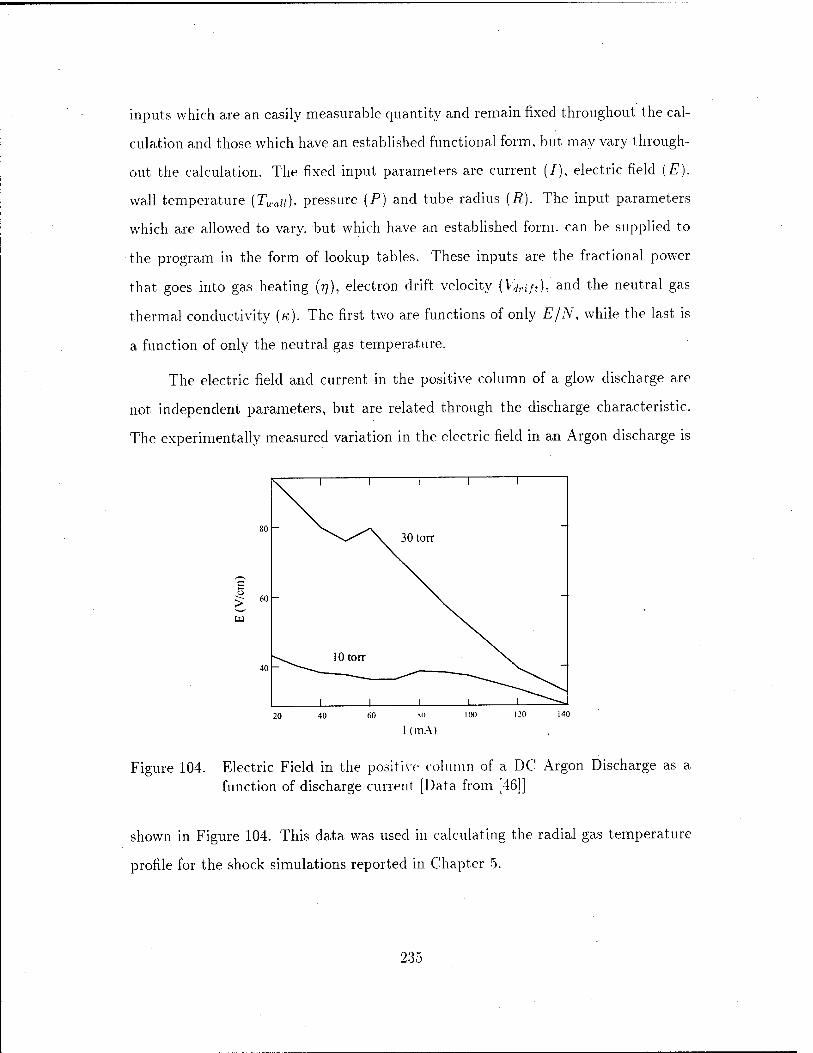
inputs which are an easily measurable quantity and remain fixed throughout the cal-

culation and those which have an established functional form, but may vary through-

out the calculation. The fixed input parameters are current (/), electric field (£),

wall temperature [TwaU), pressure (P) and tube radius {R). The input parameters

which are allowed to vary, but which have an established form, can be supplied to

the program in the form of lookup tables. These inputs are the fractional power

that goes into gas heating (77), electron drift velocity (Vdrift), and the neutral gas

thermal conductivity (K). The first two are functions of only E/N, while the last is

a function of only the neutral gas temperature.

The electric field and current in the positive column of a glow discharge are

not independent parameters, but are related through the discharge characteristic.

The experimentally measured variation in the electric field in an Argon discharge is

6

W

80

60 -

40 -

1 1 1 1 1

30 torr

10 torr

1 1 1 1 1 ^~^~-~^

40 120

(ITlA)

Figure 104. Electric Field in the positive column of a DC Argon Discharge as a function of discharge current [Data from [46]]

shown in Figure 104. This data was used in calculating the radial gas temperature

profile for the shock simulations reported in Chapter 5.

235

The data that can be supplied to the model in terms of lookup tables are

■i] (the fraction of the total power going into gas heating), Vdrift (drift velocity of

the electrons in the positive column due to the axial electric field) and K (thermal

conductivity of the neutral gas). The former two are shown in Figures 105 and

Figure 105. r\ (fractional power into gas heating) vs E/N in Argon (points were determined from numerical solution to Boltzmann's equation [97]; solid curve is a cubic spline fit to points)

106 as functions of E/N in Argon (E/N is in units of Townsend, where 1 Td = 1.0

xlO-17 Volt-cm2). The data points in these figures were extracted from a numerical

solution to the Boltzmann equation, using the Bolsig code [97]. Bolsig was run for a

broad E/N range (1-100 Td), with the resulting transport coefficients cross-checked

using an independent Boltzmann solver [17] to ensure accuracy. The solid curves

in these figures represent a cubic spline fit to the data points and were used in the

thermal model.

The thermal conductivity of Argon as a function of temperature is shown in

Figure 107. The points in this figure were taken from tables in [5] while the solid

curve is used in the thermal model to represent the thermal conductivity.

236

Figure 106. Vdrift (electron drift velocity) vs E/N in Argon (points were determined from numerical solution to Boltzmann's equation [97]; solid curve is a cubic spline fit to points)

_ 1 1 1 1 d" M o <l> C/3

g W) 0 06 -/ — M ^~* c? > o 3 -o o 0 04 — y^ —

U 03

(1) J3 H

0.02, W\ 1 1 i i- 500 1000 1500 2000

Gas Temperature (K) 2500

Figure 107. Thermal Conductivity in Argon [kg m/sec3/K

237

D.6 Test Cases and Typical Results

Results of the thermal model were compared to peak temperatures from pre-

vious calculations as reported in the literature. These comparisons are summarized

in Table 1. where the peak temperatures from the present model are listed in the

last column and the peak temperatures from previous calculations are listed in the

next to last column. The agreement between the two is quite good, with less than

1% relative difference. The other entries in this table define the parameters of the

calculation and are inputs into the present model (shown for clarity).

Table 1. Test Cases: Results of thermal model in Argon

Source I (mA) E (V/cm) R (cm) P (torr) Twall (K) r^*(K) ?S(K) [391 250 1.377 0.4 10 340 525 529

[39] 250 1.50 0.4 5 344 543 547

r (normalized)

Figure 108. Intermediate T(r) profiles corresponding to the 1=100 mA case in [46].

238

A typical sequence of intermediate T(r) profiles is shown in Figure 108 calcu-

lated for the 1=100 mA case in [46] (Argon, / = 100 mA, E = 51.5 V/cm, R = 2.5

cm. P = 30 torr). This case took 35 iterations through the algorithm to converge.

with the numbers shown in the figure corresponding to the iteration number. The

curve labeled 1 is the initial guess (a J0 Bessel function with a peak temperature of

950 K). The curve labeled 35 is the final converged solution. It is apparent there

is little deviation between the solutions of successive iterations as the converged

solution is approached.

W

Figure 109. Calculated E/N ratios along centerline (curve 1) and along the tube wall (curve 2) for an Argon discharge at 30 torr (input parameters from [46]).

Using the electric field values determined experimentally for an Argon discharge

at 30 torr (Figure 104) and the temperatures as determined by the thermal model,

the E/N ratios along the centerline and tube wall can be calculated (see Equation

165). The result is shown in Figure 109, where curve 1 represents the E/N ratio (in

239

units of Tel) along the centerline and curve 2 the same quantity along the tube wall.

The E/N ratio is not a constant, but can vary from a maximum of approximately

18 Td (on the centerline for a current of 60 mA) to a minimum of approximately 4

Td (at the wall for a current of 140 mA): a factor of more than 4. Since the wall

temperature in these calculations was assumed to be a constant (300A'). the E/N

ratio along the wall simply reflects the discharge characteristic as given in Figure

104. The calculation of the E/N ratio along the centerline, however, takes into

account both the discharge characteristic and the centerline temperature, each of

which varies with current.

The strength of the present thermal model is that all its inputs are parameters

which are either readily controlled or measured by the experimenter. Other thermal

models [[39], [41]] require the user to specify parameters over which the experimenter

has no control, such as the fraction of the total power going into gas heating (?/).

In the present model, 77 is determined at each radial location by the local value of

the E/N ratio, using the results from a Boltzmann equation solver in the process.

Additionally, the source term used in the calculation (RHS of equation 159) is con-

sistent at all times with the total discharge current. The algorithm upon which the

present thermal code is based should be applicable in cases in which the local (or 0-D

Boltzmann) model of the plasma holds and in which the wall temperature (-T^i)

of the discharge tube can be specified as a constant. While rwaji may continue to

rise over time until a true steady-state is achieved, it can be considered to be con-

stant over the time in which a shock propagates through the discharge. Therefore,

it should be applicable in the positive column of the discharge. Finally, the effect of

the convective flow of gas has not been included in this gas heating model.

240

Appendix E. Optical Diagnostics in Shock Tubes: A Short Tutorial

Optical measurements are frequently made in shock tubes clue to their non-

intrusive nature. That is, measurements can be made without inserting probes into

the shock tube that would otherwise interfere with the gaseous flow. Both den-

sity and density gradient measurement techniques have been used in investigating

plasma/shock interactions and each relies on a different physical principle. Under-

standing these principles is essential in order to compare the results of numerical

simulations to the measured data.

Although optical measurement techniques applied to shock waves are probably

well known in certain settings, it was a new field to the author, and as such provided

some difficulty in understanding the data reported in the literature. Accordingly, a

good measure of time was spent in researching the various techniques in an effort

to determine the manner in which the simulated data should be sampled in order

to provide a meaningful comparison to experimental results. The purpose of the

present appendix is not to replace the existing volumes of literature on the subject

of optical shock diagnostics, rather, the intent is to provide a short tutorial of two

optical techniques commonly employed and to provide enough references to send the

interested reader in the proper direction to get more information.

Although many optical methods are available for shock tube diagnostics, only

those methods used in experiments which were numerically simulated in the present

research will be discussed. These methods are optical interferometry and photo-

acoustic deflection spectroscopy (PADS). Using a Riemann problem as a basis, both

of these techniques will be addressed and a sample of the simulated data provided

by each will be shown.

241

E.l Optical Interferometry

HAU» SILVeRtD MIMOII

UCHT SOUftCC

^xn \

HALF ilLVCMO MMROR

COMPINSATMG «.AT«

PHOTOCHAMM

Figure 110. Typical Mach Zehnder interferometer used in shock tube diagnostics

[118].

According to Wright [118:49], the interferometer is 'undoubtably the best

method of obtaining quantitative information about the density profile of the flow in

a shock tube.' A Mach Zehnder interferometer is shown in Figure 110. A monochro-

matic light source of wavelength A is split into two legs, only one of which traverses

the shock tube. The other leg is designed to have the same optical path as the first,

using glass plates to compensate for the optical path difference and dispersion in-

troduced by the shock tube windows. Any density change from ambient {Ap) in the

shock tube portion of the path causes a change in the refractive index (An) at the

same location. That is, since the density and refractive index are related through

n = 1 + A/9, 1175)

242

where A' is known as the Gladstone Dale constant (see [118:41] for typical values),

the changes are also related, in that

An = A'A/r». (176)

The optical path length is increased by Y'An (where Y is the width of the shock

tube), which can be equated to an integral number of wavelengths (iVA). Thus, the

change in density can be determined by the number of fringes which are observed as

the shock passes, according to

N=J^-Ap. (177)

In general, the density change across the shock tube can be a function of position,

that is, A/9 = Ap(y), where y is the transverse coordinate. Such would be the case if

a transverse thermal gradient were present, for example. In this case, the number of

fringes observed would be determined by the integrated value of the density change

at each transverse position, given by

A' N=jJQ Ap(y)dy. (178)

Thus, one sees a difficulty emerging in that while the number of fringes can be

measured, the density change inferred from this measurement is a quantity averaged

over the width of the shock tube. Accordingly, the density that is reported in the

literature using this technique can be described as an average density, defined as

1 fy

i Jo

where t denotes time. In the two-dimensional numerical simulations of experiments

using the interferometry technique, Equation 179 was used to sample the computed

density field at each time step of the calculation.

243

-o m N

Q. 2 -

4 1 1 1

contact surface

3

shock front

/ \/

| —

2 -/ -

1 _^

1

1 1 1 400 600 800

time (usec)

Figure 111. Typical simulated signal resulting from the application of the interferometer measurement technique (equation 179) to a two-dimensional Riemann problem for a shock in gas at 300A'.

Using the Riemann problem as a basis, the temporal variation of the transverse-

averaged density (according to Equation 179) is shown in Figure 111. The shock tube

used in this example is 100 cm long with a width of 5 cm. The diaphragm is initially

located at 40 cm and Equation 179 was applied transversely at a longitudinal loca-

tion of 60 cm. The initial pressure and temperature ratios in the shock tube were

10.0 and 1.25, respectively, resulting in a Mach 1.6 shock in Argon. The tempera-

ture on the low pressure side of the diaphragm is 300A'. The sharp initial rise in

the curve is due to the passage of the shock wave front. The average density (nor-

malized by the upstream ambient density) rises to a level of 1.84, consistent with

the Rankine-Hugoniot relations under the given conditions. The density remains

relatively constant at this level until the passage of the contact surface. Ideally, the

rise associated with the contact surface would also be very steep, however numerical

dissipation from the computational algorithm causes this region to be diffuse. This

is typical of many computational algorithms in the contact surface region.

244

-o

o c

3 -

2 -

1 -

contact surface

thermal contact

shock surface front

400 600 800 time ((isec)

1000

Figure 112. Typical simulated signal resulting from the application of the interferometer measurement technique (equation 179) to a two- dimensional Riemann problem for a shock in gas with a radial thermal inhomogeneity.

As another example, the case in which a radial thermal inhomogeneity is

present will be considered. Here, the conditions are exactly the same as in the

previous example, except a heated region is present, starting 10 cm from the di-

aphragm on the low pressure side. The region is heated according to Equation 88

with To = 300A" and T\ = 200A'. The temporal variation in the average density is

shown in Figure 112. The rise in the density at the shock front is not as sharp as in

the previous example. This is due to the curvature of the shock front resulting from

the transverse thermal inhomogeneity. The density reaches a localized maximum,

then decreases until passage of the thermal contact surface (see Chapter V). Another

steady rise in the density is associated with the passage of the contact surface.

245

E.2 Photo-Acoustic Deflection Spectroscopy

The photo-acoustic deflection spectroscopy (PADS) technique also relies on the

principle of an index of refraction change caused by the passage of a shock wave,

but in a completely different way from the interferometer. In the PADS technique,

laser light traverses the shock tube at normal incidence to the tube walls, as shown

in Figure 113. A passing shock wave produces density gradients in the x direction

resulting in gradients in the index of refraction in the x direction as well. For

Figure 113. Deviation of a light beam by a refractive index gradient, as used by photo-acoustic deflection spectroscopy (adapted from [118]).

example, behind the shock the density is higher than in front of the shock, thus

the optical path length is greater in this region than in front of the shock. This

larger path length results in the wavefront being deflected from the normal. This

deflection is not limited to the wave front only, as the Poynting vector of the wave

is also deflected. Thus, the laser beam is deflected from the normal. The amount by

which the optical path length is changed can be expressed as [118:46]

dy = Y—dx, dx

(180)

246

thus small angular deflections (« dy/dx)ca,n be expressed as

t = Y%-. (181) ax

In general, the longitudinal gradient of the index of refraction can be a function

of position, thus V±n — Vj.n(y), where the symbol J_ indicates the gradient is to

be computed in the x direction, which is perpendicular to the initial direction of

the laser beam. This would happen in the case of a shock propagating through a

transverse thermal inhomogeneity, for example. In this case, Equation 181 would

become

B= /* V±n(y)dy, (182) Jo

which is, to within a constant of the order of unity, equivalent to the expression given

in [96:507]. Making use of the relationship between index of refraction and density

(Equation 175), Equation 182 becomes

6 = K [\±p(y)dy, (183) Jo

indicating the linear relationship between angular deflection and the integrated value

of the transverse density gradient.

Experimentally, it is common practice to use a single detector to measure the

laser beam deflection ([96], [46], [95], for example). This is made possible by use of

either a knife edge (as in [96]) or a slit (as in [46] and [95]), which blocks a portion of

the beam from the detector. According to [96], the voltage from the photodetector

in such an arrangement will be according to

AV = Vberf(\/20/0), (184)

where erf is the error function, V0 is the signal from the photodetector under ambient

conditions and <j> is the divergence angle from the laser, given as <f> = \/(nw0).

247

where w0 is the beam waist. For small deflection angles, the photodetector signal

is proportional to the deflection angle, as given by Equation 183. Notice, however,

that the beam deflection can be either positive or negative, according to whether

the integrated density gradient is either positive or negative. More information on

the photo-acoustic deflection technique can be found by in [7], [30], [67], [95], [100],

[104], [107] and [122].

c 3

I ca

C SP c/5 o

o u <

I 2 o

JS OH

T

6 -

4 -

2 -

shock front

contact surface

Lu 400 600 800

time (usec) 1000

Figure 114. Typical simulated signal resulting from the application of the photo- acoustic deflection measurement technique (equation 184) to a two- dimensional Riemann problem for a shock in gas at 300Ä".

As an example of this technique, consider a Riemann problem in which the

shock propagates into Argon at a uniform temperature of 300A". The shock tube

configuration is the same as given previously. The temporal variation of the photo-

acoustic signal, which has been assumed to be proportional to the laser deflection

angle given by Equation 183, is shown in Figure 114. The sharp spike at approxi-

mately 400 ^sec is due to passage of the shock wave front. The width of this signal

is an indication of the width of the shock front. Behind the shock front, the density

is relatively constant, as shown in Figure 111. The passage of the contact surface

results in another signal, starting at approximately 800 ^sec. This signal is broader

248

in time than that associated with the shock front. This is a result of the numerical

dissipation in the contact surface region mentioned previously in this appendix.

a 3

£ A-

•e C3

e 60

c7i

3 O

O

contact surface

shock front


400 600

time ((isec) 1000

Figure 115. Typical simulated signal resulting from the application of the photo- acoustic deflection measurement technique (equation 184) to a two- dimensional Riemann problem for a shock in gas with a radial thermal

inhomogeneity.

As a final example, consider the case in which the shock propagates into a

region with a transverse thermal inhomogeneity, defined exactly as before. The

temporal variation of the photo-acoustic signal in this case is shown in Figure 115.

Again, a sharp spike is present in the signal which is associated with passage of the

shock front. However, the structure of this spike is different in this case, due to the

curvature of the shock front in the presence of a thermal inhomogeneity. Broader

signals associated with the thermal contact surface and contact surface are also

shown.

249

Bibliography

1. Abe, Kanji and Gyo Sakaguchi. "Linear and Nonlinear Evolution of Double- humped Ion Distributions in Strong Unmagnetized Shock Structures," The Physics of Fluids, ££(12):3581-3589 (December 1985).

2. Aleksandrov, A.F., et al. "A possible mechanism for interaction of a shock wave with a decaying plasma in air," Sov. Phys. Tech. Phys., 37(4):468-469 (April 1986).

3. Anderson, Dale A., et al. Computational Fluid Mechanics and Heat Transfer. Hemisphere Publishing Corporation, 1984.

4. Anderson, Jr., John D. Introduction to Flight. New York: McGraw-Hill, Inc.,

1978.

5. Anderson, Jr., John D. Hypersonic and High-Temperature Gas Dynamics. New York: McGraw-Hill, Inc.. 1989.

6. Avramenko, R.F., et al. "Structure of a shock wave in a weakly ionized nonisothermal plasma," JETP Lett., ,^(9):463-466 (1981).

7. Azzeer, A.M., et al. "Optical probing of laser-induced shock waves in air," Appl. Phys. B, £3:307-310 (1996).

8. Bailey, William F. Collision induced dissociation of diatomic molecules. PhD dissertation, Air Force Institute of Technology. Wright-Patterson AFB, OH, 1978.

9. Baksht, F.G. and G.I. Mishin. "Effects of vibrational relaxation on the parameters of shock waves in a molecular gas plasma," Sov. Phys. Tech. Phys., 25(5):547-549 (May 1983).

10. Barkhudarov, E.M., et al. "Dissipation of a weak shock wave in a laser spark in air," Sov. Tech. Phys. Lett., iO(10):4<)8-499 (October 1984).

11. Basargin, I.V. and G.I. Mishin. "Probe studies of shock waves in the plasma of a transverse glow discharge," Sor. Tfch. Phys. Lett, 11 (ll):535-538 (1985).

12. Basargin, I.V. and G.I. Mishin. "Shock-wave propagation in the plasma of a transverse glow discharge in argon." Sov. Tech. Phys. Lett., 11 (2):Sö-S7

(1985).

13. Basargin, I.V. and G.I. Mishin. "Precursor of shock wave in glow-discharge plasma," Sov. Tech. Phys. Lett, 1-5(4):311-313 (1989).

14. Basargin, I.V. and G.I. Mishin. "Evolution of anomalous dynamic properties of a decaying glow-discharge plasma," Tech. Phys., ^l(7):742-744 (1996).

15. Beam, R.M. and R.F. Warming. "An Implicit Finite-Difference Algorithm for Hyperbolic Systems in Conservation Law Form," ./. Comp. Phys., 52:87-110 (1976).

250

16. Beclin, A.P. and G.I. Mishin. "Ballistic studies of the aerodynamic drag on a sphere in ionized air.1' Tech. Phys. Lett., 21{l):5-7 (January 1995).

17. Bennett, Eric, "Bolt — A Time - Dependent Bolzmann Solver." Unpublished, July 1996. Air Force Institute of Technology, Wright-Patterson AFB, OH.

18. Beran, Philip S., "Aero752 Lecture Notes." 1997. AERO 752 - Computational Aerodynamics, Air Force Institute of Technology, Wright-Patterson AFB, OH.

19. Bhatnagar, P.L., et al. "A Model for Collision Processes in Gases. I. Small Am- plitude Processes in Charged and Neutral One-Component Systems," Physical

Review, 94:511 (1954).

20. Bletzinger, Peter. Private Communication, 1997. Wright Laboratory (WL/POO), Wright-Patterson AFB, OH.

21. Bond, Jr., John W., et al. Atomic Theory of Gas Dynamics. Reading, Mass.: Addison-Wesley, 1965.

22. Bond, Jr., J.W. "Plasma Physics and Hypersonic Flight," Jet Propulsion, 228-235 (April 1958).

23. Boris, J.P. and D.L. Book. "Flux Corrected Transport I, SHASTA, a Fluid Transport Algorithm that Works," Journal of Computational Physics, 11:38-

69 (1973).

24. Bray, K.N.C. "Vibrational relaxation of anharmonic oscillator molecules: relaxation unber isothermal conditions," ./. Phys. B (Proc. Phys. Soc), 1:705 (1968).

25. Brown, Garry, "Hypersonic Flow Control." Plasma-Based Hypersonic Drag Reduction Workshop, Wright-Patterson AFB, OH, May 1996.

26. Buyanova, E.A., et al. "Stationary Shock Waves in a Nonequilibrium Diatomic Gas," Sov. J. Chem. Phys., 1 (12):2856-2860 (1984).

27. Bystrov, S.A., et al. "Propagation of Plane Shock Wave in Weakly Ionized Plasma," Sov. J. Plasma Phys., i5(5):324-326 (1989).

28. Bystrov, S.A., et al. "Precursor ahead of a shock front in an rf discharge plasma," Sov. Phys. Dokl, 35(l):39-40 (1990).

29. Cambel, Ali Bulent. Plasma Physics and Magnetofluiddynamics. New York: McGraw-Hill Book Co., 1963.

30. Casperson, Lee W. "Gaussian Light Beams in Inhomogeneous Media," Applied Optics, li?(10):2434-2441 (1973).

31. Cherrington, B.E. Gaseous Electronics and Gas Lasers. New York: Pergamon Press, 1979.

32. Chutov, Yu.I. "Experimental Investigation of Shock Waves in a Partially Ion- ized Discharge Plasma," Zhurnal Prikladnoi Mekhaniki i Tekhnicheskoi Fiziki,

11 (1)424-130 (1970).

251

33. Chutov, Yu.I. and V.N. Podolskii. "Shock Waves in a Gas-Discharge Plasma," Journal of Engineering Physics and Thermophysics, #2(5):504-509 (May 1992).

34. Chutov, Yu.I., et al. "Explosive waves in an evolving gas discharge," Sov. Tech, Phys. Lett., i7(2):101-102 (February 1991).

35. DeJoseph, Jr., CA., "N2 Kinetic Vibration Code." Private Communication, 1997. Wright Laboratory (WL/POO), Wright-Patterson AFB, OH.

36. Dendy, Richard. Plasma Physics: An Introductory Course, Cambridge: Cam- bridge University Press, 1993.

37. Dolgov. G.G. and S.L. MandeFshtam. "Density and temperature of a gas in a spark discharge," Zh. Eksperim. i Teor. Fiz., 1^:691-700 (1953).

38. Drabkina, S.I. "The theory of the development of a spark discharge column," Zh, Eksperim. i Teor. Fiz., 21:473^483 (1951).

39. Eden, J.G. and B.E. Cherrington. "Radial neutral gas temperature and density profiles in low-pressure argon discharges," ./. Appl. Phys., ^(ll):4920-4926 (November 1973).

40. Emanuel, G. Gasdynamics: Theory and Applications. New York: American Institute of Aeronautics and Astronautics, 1986.

41. Evtyukhin, N.V., et al. "On the Nature of Shock Wave Acceleration in Glow Discharge Plasma," Sou. J. Chem. Phys., 2(9):2080-2089 (1986).

42. Evtyukhin, N.V., et al. "Shock Waves in a Vibrationally Excited Gas," Sov. J. Chem. Phys., ^ (9):2100-2108 (1987).

43. Feynman, Richard P., et al. The Feynman Lectures on Physics, II. Reading, Massachusettes: Addison-Wesley Publishing Company, Inc., 1964.

44. Fletcher, C.A.J. Computational Techniques for Fluid Dynamics. Berlin: Springer-Verlag, 1991.

45. Ganguly, B.N., "Private Communication," 1997. Wright Laboratory (WL/POO), Wright-Patterson AFB, OH.

46. Ganguly, B.N. and P. Bletzinger. "Shock Wave Dispersion in Nonequilibrium Plasmas," AIAA Paper 96-4607 (1996).

47. Godunov, S.K., "A difference scheme for numerical computation of discontinuous solution of hydrodynamic equations." Math. Sbornik, 47:271-306 (in Russian). Translated in US Joint Publ. Res. Service, JPRS 7226 (1969).

48. Gordeev, V.P., et al. "Experimental Study of the Possibility of Reducing Su- personic Drag by Employing Plasma Technology," Fluid Dynamics, 31 (2):313~ 317 (1996).

49. Gordiets, Boris F., et al. Kinetic Processes in Gases and Molecular Lasers. New York: Gordon and Breach Science Publishers, 1988.

252

50. Gorshkov, V. A., et al. "Behavior of electron density in a wakly ionized nonequilibrium plasma with a propagating shock wave," Sov. Phys. Tech. Phys.,

S£(10):1138-1141 (October 1987).

51. Grachev, L.P., et al. "Interaction of a shock wave with a decaying plasma in an electrodeless microwave discharge," Sov. Phys. Tech. Phys., 30(5):586-588 (1985).

52. Gridin, A.Yu., et al. "Propagation of Shock Waves in a Nonuniform Transverse Pulsed Discharge," High Temperature, 32(4):454-457 (1994).

53. Gridin, A.Yu., et al. "Two-Dimensional Simulation of Shock Wave Propaga- tion in a Transverse Pulse Glow Discharge with a Heated Cathode Layer," High Temperature, S2(6):755-758 (1994).

54. Gridin, A.Yu., et al. "Structure of a shock wave in the plasma of a non- steady-state glow discharge with ultraviolet irradiation," 50t'. Tech. Phys. Lett., i£(4):295-297 (1990).

55. Gridin, A.Yu., et al. "Propagation of shock waves in the plasma of a glow discharge." Technical Physics, SS(3):238-240 (March 1993).

56. Gureev, K.G. and V.O. Zolotarev. "Evolution of the molecular vibrational distribution function and the structure of the flow in the relaxation zone behind a stationary shock front in a vibrationally excited molecular gas," Sov. Phys. Tech. Phys., 35(2):149 (February 1990).

57. Gurijanov, Evgeniy P. and Philip T. Harsha. "AJAX: New Directions in Hy- personic Technology," AIAA Paper 96-4609 (November 1996).

58. Harsha, Philip T. Private Communication, August 1997. Hypersonics Division, North American/Boeing.

59. Harten, A. "High Resolution Schemes for Hyperbolic Conservation Laws," Journal of Computational Physics, 5:357-393 (1983).

60. Hasegawa, Masaaki. "Amplification of Sound Waves in Partially Ionized Gases," Journal of the Physical Society of Japan, 57(1):193-199 (July 1974).

61. Hirsch, Charles. Numerical Computation of Internal and External Flows. New York: John Wiley and Sons, 1990.

62. Hoffmann, Klaus A. and Steve T. Chiang. Computational Fluid Dynamics for Engineers. Wichita, Kansas: Engineering Education System, 1993.

63. Ingard, Uno and Kenneth W. Gentle. "Longitudinal Waves in a Weakly Ionized Gas," The Physics of Fluids, 5:1396-1397 (1965).

64. Ingard, Uno and Michael Schulz. "Acoustic Wave Mode in a Weakly Ionized ' Gas," Physical Review, i55(l):106-lll (1967).

253

65. Ingard, Uno and Michael Schulz. "Ion Density and Electric-Field Perturbations Caused by an Acoustic-Wave Pulse in a Weakly Ionized Gas," Phys. Fluids,

li:106-lll (June 1967).

66. Ingold, John. Private Communication, 1997.

67. Jackson, W.B., et al. "Photothermal deflection spectroscopy and detection." Applied Optics, <2tf (8): 1333-1344 (1981).

68. Jaffrin, Michel Y. "Shock Structure in a Partially Ionized Gas," The Physics

of Fluids, £(4):606-625 (1965).

69. Jaffrin, Michel Y. and Ronald F. Probstein. "Structure of a Plasma Shock Wave," The Physics of Fluids, 7(10):1658-1674 (October 1964).

70. Jones, W.D., et al. An Introduction to the Linear Theories and Methods of Electrostatic Waves in Plasmas. New York: Plenum Press, 1985.

71. Kandebo, Stanley W. "'Air Spike' Could Ease Hypersonic Flight Problems," Aviation Week and Space Technology, ^2:66-67 (May 1995).

72. Keck, J.C. and G. Carrier. "Diffusion Theory of Nonequilibrium Dissociation and Recombination," Journal of Chemical Physics, 43:2284 (1965).

73. Klimov, A.I. Private Communication, April 1996. Flow Control Through Plasma Effects, Windows on Science Lecture, Wright-Patterson AFB, OH.

74. Klimov, A.L, et al. "Shock wave propagation in a decaying plasma," Sov. Tech, Phys. Lett.. £(5):240-241 (1982).

75. Klimov, A.I., et al. "Shock wave propagation in a glow discharge," Sov. Tech, Phys. Lett., 0(4):192-194 (1982).

76. Klimov, A.I. and G.I. Mishin. "Interferometric studies of shock waves in a gas-discharge plasma," Sov. Tech. Phys. Lett, l£(12):960-962 (1990).

77. Klimov, A.I., et al. "Propagation of shock waves in a non-steady-state discharge," Sov. Tech. Phys. Lett, J5(10):800-802 (1989).

78. Landau, L. and E. Teller. "Zur Theorie der Schalldispersion," Physik Z. Sow-

jetunion, b. 10(h. 1):34 (1936).

79. Landau, L.D. and E.M. Lifshits. Fluid Mechanics. London: Pergamon Press,

1959.

80. Lu, C.S. and A.B. Huang. "Shock-Wave Structure in a Partially Ionized Gas," The Physics of Fluids, !7(8):1527-1534 (August 1974).

81. Lusczek, Jr., Joseph J., et al., editors. Proceedings of the Hypersonics: The New Physics Conference, ASC-TR-97-5013, 1997.

82. MacCormack, R.W. "The Effect of Viscosity in Hypervelocity Impact Crater- ing," AI A A Paper 69-354 (1969).

254

83. Maksimov, A.I., et al. "Thermocouple measurements of the gas temperature in a glow discharge," Sov. J. Plasma Phys., j(2):194-197 (1978).

84. Millikan. Roger C. and Donald R. White. "Systematic^ of Vibrational Relax- ation," The Journal of Chemical Physics, 5P(12):3209-3213 (December 1963).

85. Mishin, G.I. "Shock waves in a weakly ionized nonisothermal plasma," Sov. Tech. Phys. Lett., n(3):112-114 (1985).

86. Mishin, G.I. Gas Dynamics, chapter Sonic and Shock Wave Propagation in Weakly Ionized Plasma. Commack, New York: Nova Science Publishers, Inc.,

1992.

87. Mishin, G.I. "Total pressure behind a shock wave in weakly ionized air," Sov.

Tech. Phys. Lett, £0(ll):857-859 (1994).

88. Mishin, G.I., et al. "Anomalous relaxation and instability of shock waves in gases," Sov. Tech. Phys. Lett, i?6(ll):1363-1368 (1981).

89. Mishin, G.I., et al. "Measurements of the pressure and density in shock waves in a gas discharge plasma," Sov. Tech. Phys. Lett., J7(8):602-604 (1991).

90. Mishin, G.I., et al. "Flow around a sphere moving supersonically in a gas- discharge plasma," Sov. Tech. Phys. Lett., i7(6):413-416 (1991).

91. Mott-Smith, H.M. "The Solution of the Boltzmann Equation for a Shock Wave," The Physical Review, £2(6):885-892 (June 1951).

92. Newell, Alan C., et al., "Can One Use A Plasma Sheath Around Hypersonic Vehicles to Improve Flight Characteristics?." Plasma-Based Hypersonic Drag Reduction Workshop, Wright-Patterson AFB, OH, May 1996.

93. Osipov, A.I. and A.V. Uvarov. "Kinetic and Gasdynamic Processes in Nonequilibrium Molecular Physics." Sov. Phys. Usp., 35(ll):903-923 (Novem- ber 1992).

94. Peterkin, Jr., Robert E. and Captain Dennis E. Lileikis, ^'Simulating Plasma- Magnetic Field Interactions for Boundary Layer Control in Hypersonic Flight." Plasma-Based Hypersonic Drag Reduction Workshop, Wright-Patterson AFB,

OH, May 1996.

95. Petzoldt, S., et al. "Surface laser damage thresholds determined by photacous- tic deflection," Appl. Phys. Lett., .>./(2I):200ö-2007 (1988).

96. Pini, R., et al. "Probe-beam deflection diagnostics of shock waves generated during laser drilling," Appl. Phys. B. 67:505-510 (1995).

97. Pitchford, L.C. and W.L. Morgan, "Bolsig Version 1.05 Electron Boltzmann Equation Solver," 1996. Freeware.

98. Raizer, Yu. P. Gas Discharge Physics. Berlin: Springer-Verlag, 1991.

99. Roe, P.L. "Approximate Riemann solvers, parameter vectors and difference schemes," Journal of Computational Physics, ^3:357-72 (1981).

255

100. Rose, A. and R. Gupta. "Application of photothermal deflection technique to flow-velocity measurements in a flame," Optics Letters, iö(ll):532-534 (1985).

101. Rukhadze, A.A., et al. "Propagation of Nonstationary Shock Waves in Vibra- tionally Excited Nitrogen," Soviet Physics'Lebedev Institute Report, (6):18-23

(1983)!

102. Sato, Masumi and Satoshi Arima. "Measurements of gas temperature in an argon positive column using acoustic wave propagation," ./. Phys. D: Appl. Phys., £5:1302-1306 (1990).

103. Schwartz, R.N., et al. "Calculation of Vibrational Relaxation Times in Gases," J. Chem. Phys., £0(1O):1591 (October 1952).

104. Sell, Jeffrey A., et al. "Laser beam deflection as a probe of laser ablation materials," Appl. Phys. Lett, 55(23):2435-2002437 (1989).

105. Serov, Yu.L. and I.P. Yavor. "Ablation during supersonic motion of an object in a plasma," Tech. Phys., ^0(3):24S-251 (March 1995).

106. Sessler, G.M. "Propagation of Longitudinal Waves in a Weakly Ionized Gas," The Physics of Fluids, 7(l):90-95 (January 1964).

107. Sigrist, Markus W. "Laser generation of acoustic waves in liquids and gases," J. Appl, Phys., 00(7):R83-R9O (1986).

108. Strang, G. Linear Algebra and Its Applications. New York: Academic Press,

1968.

109. Strang, G. "On the construction and comparison of difference schemes," SLAM J. Numer. Anal, 5(3):506-517 (1968).

110. Sutton, George W. and Arthur Sherman. Engineering Magnetohydrodynami.es. McGraw-Hill Book Company, 1965.

111. Tidman, D.A. "Structure of a Shock Wave in Fully Ionized Hydrogen," The Physical Review, m(6):1439-1446 (September 1958).

112. Toth, Gabor and Dusan Odstrcil. "Comparison of Some Flux Corrected Trans- port and Total Variation Diminishing Numerical Schemes for Hydrodynamic and Magnetohydrodynamic Problems," Journal of Computational Physics,

128:82-100 (1996).

113. Vidal, F., et al. "Ion Kinetic Simulations of the Formation and Propaga- tion of a Planar Collisional Shock Wave in a Plasma," The Physics of Fluids, 5(9):3182-31190 (September 1993).

114. Vincenti, Walter G. and Jr. Charles H. Kruger. Introduction of Physical Gas Dynamics. Malabar, Florida: Robert E. Krieger Publishing Company, 1965.

115. Voinovich, P.A., et al. "Propagation of Weak Shock Waves in Plasma of Lon- gitudinal Flow Discharge in Air," High Temperature, £0:468-475 (1991).

256

116. Vstovskii. G.V. and G.I. Kozlov. "Propagation of weak shock waves in a vibrationally excited gas," Sov. Phys. Tech. Phys.. 3i(8):911-914 (1986).

117. Wood, 2nd Lt, Brandon, "AEDC Tests." Unpublished, 1997. WL/POP (HyTech), Wright-Patterson AFB, OH.

118. Wright, John Keith. Shock Tubes. London: Methuen, 1961.

119. Yeager, General Chuck and Leo Janos. Yeager. New York: Bantam Books,

1985.

120. Yee, H.C. NASA TM-101088, 1989.

121. Yuschenkova, N.I., et al. "Mechanism for anomalous relaxation in shock waves in inert gases," Sov. Tech. Phys. Lett., 11 (5):215-217 (May 1985).

122. Zapka, W. and A.C. Tarn. "Noncontact optoacoustic determination of gas flow velocity and temperature simultaneously," Appl. Phys. Lett., ^0(12):1O15-1O17

(1982).

123. Zel'dovich, Ya. B. and Yu. P. Raizer. Physics of Shock Waves and High- Temperature Hydrodynamic Phyenomena, I. New York: Academic Press,

1966.

124. Zel'dovich, Ya. B. and Yu. P. Raizer. Physics of Shock Waves and High- Temperature Hydrodynamic Phyenomena, II. New York: Academic Press,

1966.

257

Vita

Major William M. Hilbun was born at Columbus AFB, MS on 12 SEP 62,

spending his youth among the rich farmlands of Mississippi. He graduated from

Tupelo High School in May 81 and entered the U.S. Air Force Academy as part of

the twenty-seventh class in June of the same year. He was graduated in May 85 with

a B.S. degree in physics and a commission as a 2nd Lieutenant in the U.S. Air Force.

His first tour of duty was with the 3246 Test Wing, Eglin AFB, FL as an infrared

(IR) test engineer, where he worked on the test and evaluation of IR guided missiles.

In May 89, he was reassigned to the Air Force Institute of Technology (AFIT) for

post-graduate studies in engineering physics. He graduated with a M.S. degree 18

months later, with his thesis work being in the area of numerical solutions to the

Boltzmann equation. Reassigned to the (then) Foreign Technology Division, Wright-

Patterson AFB, OH, Major Hilbun worked on designing, building and flight-testing

realistic re-entry vehicle decoys in support of the Strategic Defense Initiative. In

June 94, Major Hilbun entered AFIT to begin his doctoral studies in the field of

plasma aerodynamics. In October 97, he was reassigned to the Air Force Technical

Applications Center, Patrick AFB, FL. Major Hilbun is married to the former Kathi

Babbel, of Seattle, WA, and they have four children: Houston (7), Travis (5), Poiette

(4) and Tyler Davis (2).

Permanent address: 3630 Manassas Ave Melbourne, FL 32934

258

REPORT DOCUMENTATION PAGE Form Approved

OMB No. 0704-0188

Public reporting burden for this collection of information is estimated to average 1 hour per response, including the time for reviewing instructions, searching existing data sources, gathering end maintaining the data needed, and completing end reviewing the collection of information. Send comments regarding this burden estimate or any other espect of this collection of information, including suggestions for reducing this burden, to Washington Headquarters Services, Directorete for Informetion Operations and Reports, 1215 Jefferson Davis Highway, Suite 1204, Arlington, VA 22202-4302, and to the Office of Management and Budget, Paperwork Reduction Project (0704-0188), Weshington, DC 20503.

1. AGENCY USE ONLY (Leave blank! 2. REPORT DATE

October 1997

3. REPORT TYPE AND DATES COVERED

Final 4. TITLE AND SUBTITLE


6. AUTHOR(S)

William M. Hilbun, Major, USAF

5. FUNDING NUMBERS

7. PERFORMING ORGANIZATION NAME(S) AND ADDRESS(ES)

Department of Engineering Physics Air Force Institute of Technology Wright-Patterson AFB, OH, 45433-7542

8. PERFORMING ORGANIZATION REPORT NUMBER

AFIT/DS/ENP/97D-08

9. SPONSORING/MONITORING AGENCY NAME(S) AND ADDRESS(ES)

Wright Laboratory 2130 Eighth St., Ste. 1 Wright-Patterson AFB, OH, 45433-7542

10. SPONSORING/MONITORING AGENCY REPORT NUMBER

11. SUPPLEMENTARY NOTES

12a. DISTRIBUTION AVAILABILITY STATEMENT

Distribution Unlimited 12b. DISTRIBUTION CODE

13. ABSTRACT (Maximum 200 words!

An analysis and assessment of three mechanisms describing plasma/shock wave interactions was conducted under conditions typically encountered in a weakly ionized glow discharge. The mechanisms of ion-acoustic wave damping, post-shock energy addition and thermal inhomogeneities were examined by numerically solving the Euler equations with appropriate source terms adapted for each mechanism. Ion-acoustic wave damping was examined by modelling the partially ionized plasma as two fluids in one spatial dimension using the Riemann problem as a basis. Post-shock energy addition in the form of nonequilibrium vibrational energy relaxation was also examined in one spatial dimension using the Riemann problem as a basis. The influence of thermal inhomogeneities on shock wave propagation was examined in two spatial dimensions for both a Riemann shock and a shock generated by a spark discharge. Shocks were propagated through realistic thermal profiles with the resulting shock structure examined through the numerical application of various optical diagnostic techniques. Results from shock simulations indicate that ion-acoustic wave damping has an insignificant effect on the neutral flow at fractional ionization levels typical of glow discharges. Post-shock vibrational energy relaxation is also unable to effect the shock structure on the time scales of interest. An analysis of the effects of thermal inhomogeneities reveals that many of the observed plasma/shock anomalies can be explained based solely on this mechanism.

14. SUBJECT TERMS

shocks, weakly ionized plasma, ion-acoustic waves, vibrational relaxation, thermal inhomogeneities, fluid equations

15. NUMBER OF PAGES

274 16. PRICE CODE

17. SECURITY CLASSIFICATION OF REPORT

Unclassified

18. SECURITY CLASSIFICATION OF THIS PAGE

Unclassified

19. SECURITY CLASSIFICATION OF ABSTRACT

Unclassified

20. LIMITATION OF ABSTRACT

UL Standard Form 298 (Rev. 2-89) (EG) Prescribed by ANSI Std. 239.18 Designed using Perform Pro, WHS/DIOR, Oct 94

Shock Waves in Nonequilibrium Gases and Plasmas - DTIC

Documents

Transcript of Shock Waves in Nonequilibrium Gases and Plasmas - DTIC