Kinetic Theory of Gases
149
Kinetic Theory of Gases Prof.Dr. Shawky Mohamed Hassan
-
Upload
independent -
Category
Documents
-
view
3 -
download
0
Transcript of Kinetic Theory of Gases
Kinetic Theory of Gases
Prof.Dr. Shawky Mohamed Hassan
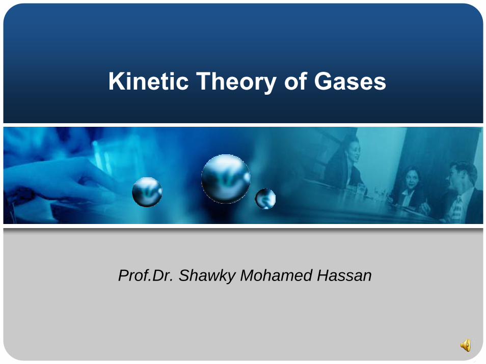
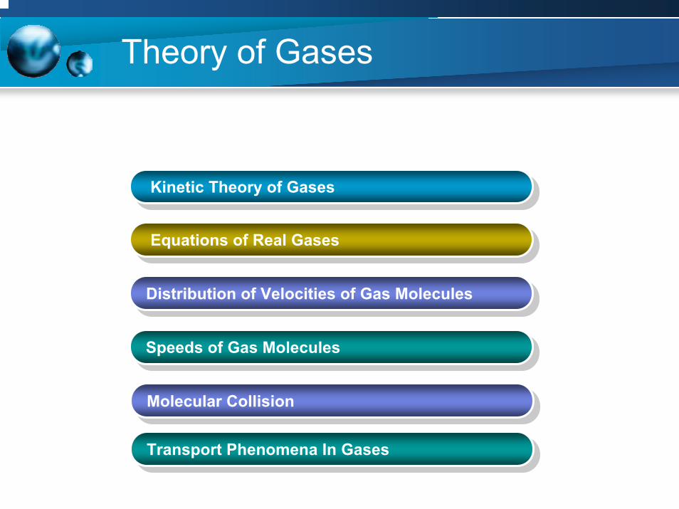
Theory of Gases
Kinetic Theory of GasesKinetic Theory of Gases
Equations of Real GasesEquations of Real Gases
Distribution of Velocities of Gas Molecules Distribution of Velocities of Gas Molecules
Speeds of Gas Molecules Speeds of Gas Molecules
Molecular CollisionMolecular Collision
Transport Phenomena In GasesTransport Phenomena In Gases
Properties of gases ( Flash animation )Properties of gases ( Flash animation )
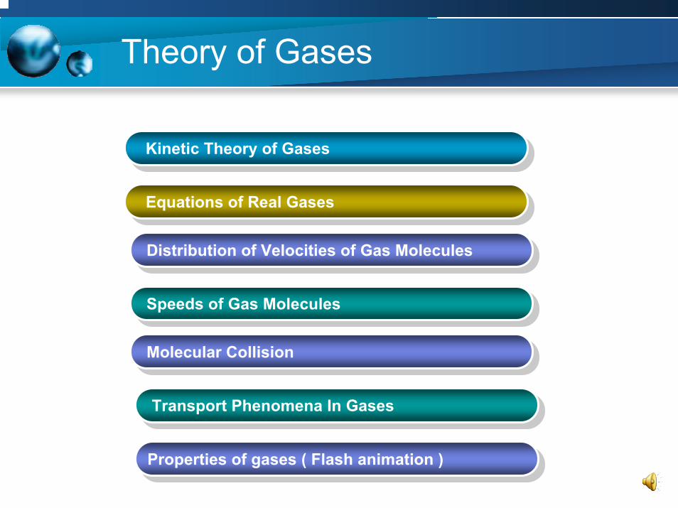
The Ideal Gas
CONTENTS
• The Ideal Gas
• Real Gases
• Distribution of Velocities of Gas Molecules
• Collision properties of gas molecules.
• Transport phenomena in gases.

Common Properties
(A) gas expands to fill its container and its volume is readily
contracts when pressure is applied.
(b) Two or more gases form homogeneous mixtures in all
proportions, regardless of how different gases may be.

Equation of State
• To define properly the state or conditions, of a gas, it is necessary to assign values to certain variable quantities –namely,
• temperature (T), volume (V), pressure (P) and quantity (n).
• The state can be specified by giving the values of any three of these variables,
• F(n,V,P,T) = 0 (1.1)
Equation of State
• Here F denotes some relationship between the variables.
• Particular forms of equations like Eq. (1.1) are called
equations of state. They can be obtained by;
(1)Fitting experimental n, V, P,T data to empirical
equations.
• Examples of these empirical equations are the followings:

Equation of State
• Law of Boyle PV = const. at const. T
• Law of Charles V/T = const. at const. P
• Law of Amontons P/T = const. at const. V
• Combined law PV/T = Const. n
• Principle of Avogadro V/n = const . at n and P
(2) Theoretical equations can be derived from models of
gases such as that proposed by the kinetic theory of
gases.
The Ideal-Gas Equation of State
• An ideal gas is defined as a gas that has the following
equation of state:
PV = nRT (1.2)
• Here R is a universal gas constant. Its units depend on
that used for P and V, since n and T have usually the units
models (mol) and degree Kelvin (K).
Note: R = PV / nT = work / nT = Energy / Mol x Kelvin

The Ideal-Gas Equation of State
A standard condition of temperature and pressure (STP)
• T = 273.15 K
• P = 101.32 k Pa (1 atm)
Using Eq.1.2 we have that;
• (The volume of one mol) = 0.022415 m3 at STP
_____________________________________________________________
Exercise
Determine the different values of R using Eq. 1.2.
V
THE MOLECULAR KINETIC THEORY OF GASES
• The properties of a prefect ideal gas can be rationalized
qualitatively in terms of a model in which the molecules of
the gas are in continuous chaotic motion.
• We shall now see how this model can be expressed
quantitatively in terms of the kinetic theory of gases.

Assumptions of the Theory
• Gases consist of discrete particles called molecules which
are of a negligible volume in comparison with that of the
container.
• The molecules are in continuous random (caotic,
Brownian) motion independent of each other (do not repel
or attract each other) and travel only in straight lines
between brief perfectly elastic collisions (no change in
kinetic energy).
Assumptions of the Theory
• The pressure of the gas is due to the collisions of
molecules.
• The kinetic energy due to the transitional motion of a mol
of gas molecules is equal to (3/2) RT.

Pressure of the Gas
• Consider N molecules of an ideal gas,
in a cubic container of side L (m).
• A typical molecule has mass m (kg), and
velocity u (ux, uy, uz) (ms-1)
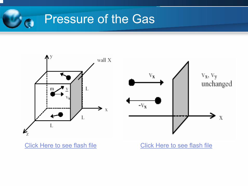
Pressure of the Gas
Click Here to see flash file Click Here to see flash file
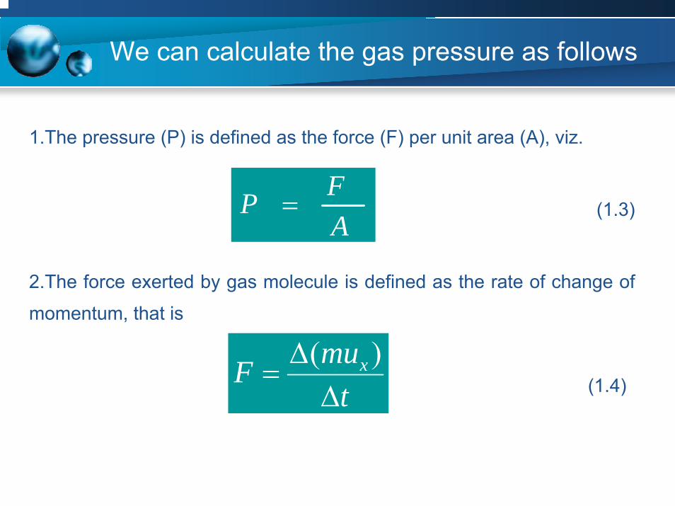
We can calculate the gas pressure as follows
1.The pressure (P) is defined as the force (F) per unit area (A), viz.
(1.3)
2.The force exerted by gas molecule is defined as the rate of change of
momentum, that is
(1.4)
AFP =
tmuF x
∆∆
=)(

We can calculate the gas pressure as follows
3. For one molecule in x direction, the momentum is mux, and change of momentum per collision = mux – (-mux)
= 2 mux (1.5)
4. Rate of change of momentum per molecule
per collision= change of momentum x number of collisions per second

We can calculate the gas pressure as follows:
•The number of collisions per second (1.6)
From Eqs. (1.1) – (1.5) we can find that the pressure on the wall A as
(1.7)
where V = L3 is the volume of the container.
•Now we can recognize that the pressure is the same for all walls of the
container. Thus we can discard the restriction “by side A”. We therefore
have
(1.8)
Lu x
2=
3
2
VmuP x
x =
1
2
VmuP x=

We can calculate the gas pressure as follows
•Now consider N molecules, instead of just one, the net pressure
becomes as
VmuNP avx )( 2
= (1.8)
We can calculate the gas pressure as follows
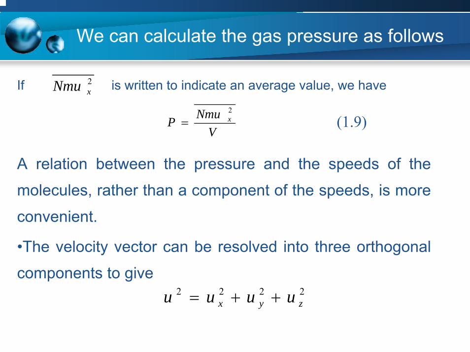
If is written to indicate an average value, we have
A relation between the pressure and the speeds of the
molecules, rather than a component of the speeds, is more
convenient.
•The velocity vector can be resolved into three orthogonal
components to give2222zyx uuuu ++=
(2.9)
(2.10)
VNmuP x
2
=
2xNmu
(1.9)
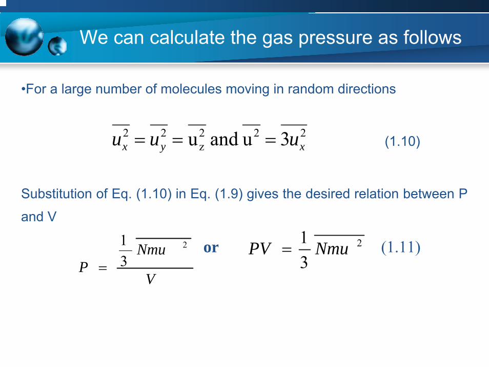
We can calculate the gas pressure as follows
•For a large number of molecules moving in random directions
(1.10)
Substitution of Eq. (1.10) in Eq. (1.9) gives the desired relation between P
and V
222z
22 3u and u xyx uuu ===
V
NmuP
2
31
=
2
31 NmuPV = (1.11)or
We can calculate the gas pressure as follows
• This important equation is as far as one can go to explain
the basis for the pressure of a gas from the four kinetic-
molecular postulates set out earlier.
• An additional postulate must be added to reach a result
that can be compared with the empirical ideal-gas laws.

Example 1.1
1 mol of O2 molecules is confined in a container and struck each of its walls each second. Calculate
(a) the total force that the molecules exert on the wall if their speed is 500 ms-1?and
(b) the pressure of the gas if the area of each wall is 20 cm2 and
(c) urms (root mean square speed) .
___________________________________________________
Solution
(a) According to Eq. (1.3) and (1.4) the force exerted by one molecule is
related to the rate of change of momentum. In 1s, the force exerted by N
molecule is
smuN
dtmuNF
12)(
=∆
∆=
smuN
dtmuNF
12)(
=∆
∆=
sxmskgxx
1))1002.6/()500)(mol 1032)(2)(1002.6( 231-1323 −−
=

Example 1.1
smuN
tmuNF
12)(
=∆
∆=
sxkgxxF
1)m.s 450)(mol 10022.6)(mol 1028)(2)(101( -1-123-1323 −
=∴= 4.2 kg.m.s-2 = 4.2 N
The corresponding pressure is
2-222 m N 4200
cm) 1/10)(cm (10N 2.4
=== − mAfP = 4200 Pa
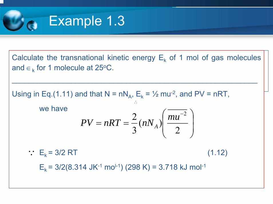
Example 1.3
Calculate the transnational kinetic energy Ek of 1 mol of gas molecules and ∈k for 1 molecule at 25oC.__________________________________________________________
Using in Eq.(1.11) and that N = nNA, Ek = ½ mu-2, and PV = nRT,
we have
Ek = 3/2 RT (1.12)
Ek = 3/2(8.314 JK-1 mol-1) (298 K) = 3.718 kJ mol-1
⎟⎟⎠
⎞⎜⎜⎝
⎛==
−
2)(
32 2munNnRTPV A
Q
∴
Example 1.3
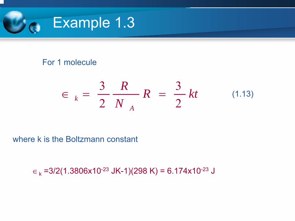
For 1 molecule
(1.13)
where k is the Boltzmann constant
∈k =3/2(1.3806x10-23 JK-1)(298 K) = 6.174x10⁻²³ J
ktRNR
Ak 2
323
==∈

Quiz 11.1 What do you understand by the terms?
(a) Chaotic motion (b) Elastic collision
(c) Ideal gas (d) Empirical Formula
1.2 State the following laws in words;
(a) T – V law, (b) T – P law,
(c) P – V law, (d) PVT law and
(e) P – n Principle.
1.3 What model of a gas was proposed by the kinetic
theory of gases.

Quiz 1
1.4 How are the following related?
(a) Torr and atm, (b) Pascal and atm,
(c) Force and pressure, (d) Pascal and joule,
(e) Gas const. and work ,and (f) Kinetic energy and
temperature.
1.5 Explain in terms of the kinetic theory of gases;
(a)Why two, given the freedom to mix, will always mix
entirely?

(b) How heating makes a gas expand at constant
pressure?.
(c) How heating a confined gas makes its pressure
increase?

Theory of Gases
Kinetic Theory of GasesKinetic Theory of Gases
Equations of Real GasesEquations of Real Gases
Distribution of Velocities of Gas Molecules Distribution of Velocities of Gas Molecules
Speeds of Gas Molecules Speeds of Gas Molecules
Molecular Collision
Transport Phenomena In Gases
Molecular Collision
Transport Phenomena In Gases
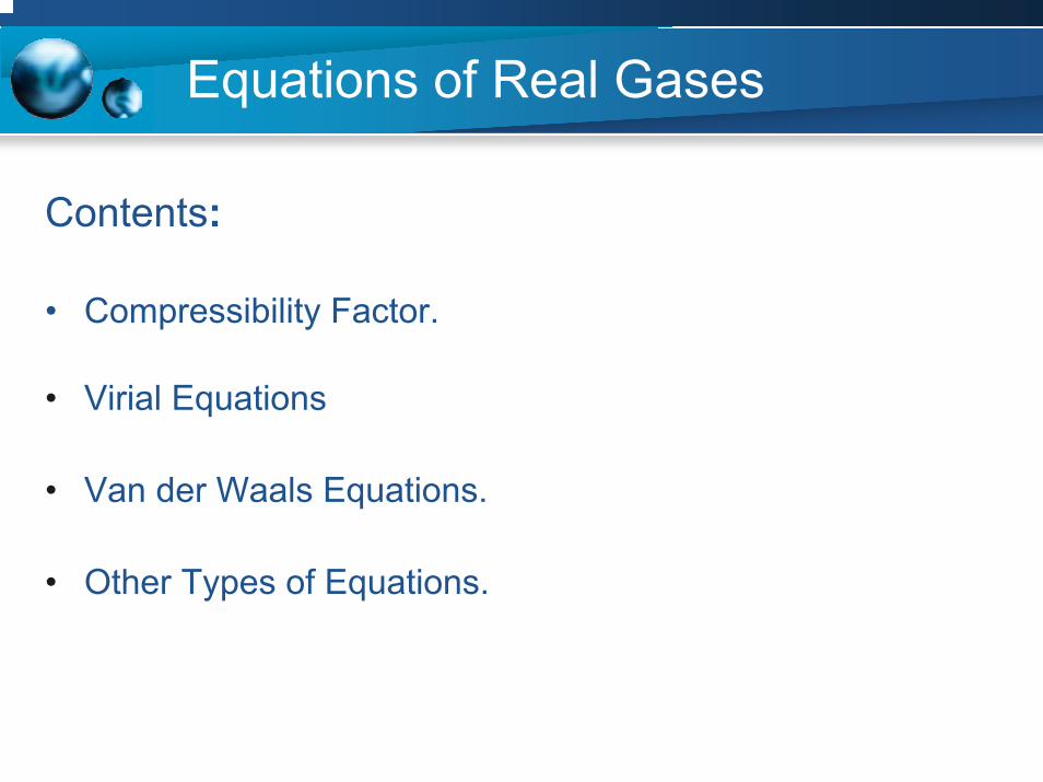
Equations of Real Gases
Contents:
• Compressibility Factor.
• Virial Equations
• Van der Waals Equations.
• Other Types of Equations.
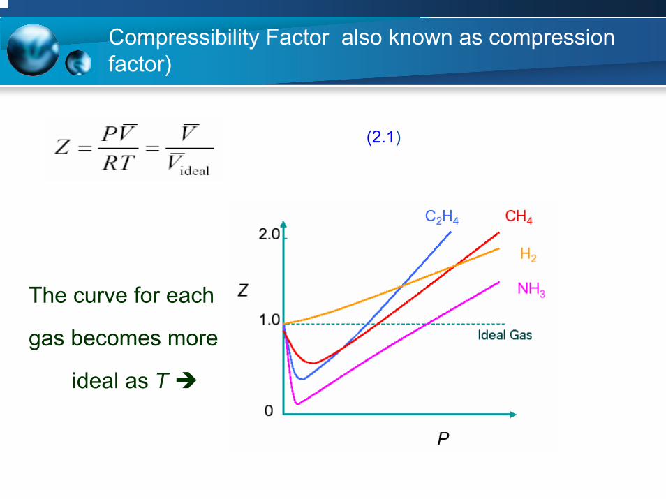
Compressibility Factor also known as compression factor)
(2.1)
The curve for each
gas becomes more
ideal as T
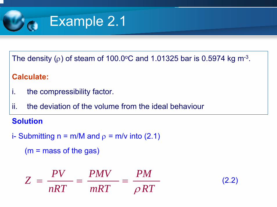
Example 2.1
The density (ρ) of steam of 100.0oC and 1.01325 bar is 0.5974 kg m-3.
Calculate:
i. the compressibility factor.
ii. the deviation of the volume from the ideal behaviour
Solution
i- Submitting n = m/M and ρ = m/v into (2.1)
(m = mass of the gas)
(2.2)RT
PMmRTPMV
nRTPVZ
ρ===
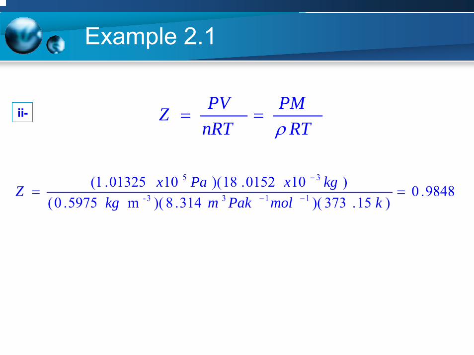
Example 2.1
RTPM
nRTPVZ
ρ==ii-
9848.0)15.373)(314.8)(m 5975.0(
)100152.18)(1001325.1(1133-
35
== −−
−
kmolPakmkgkgxPaxZ
Example 2.1
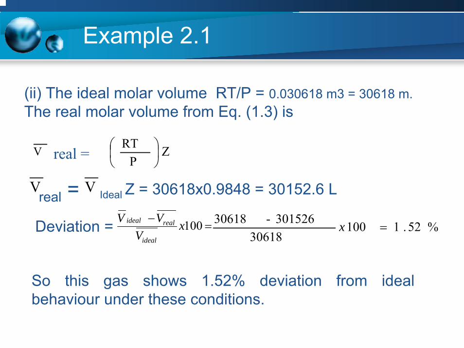
V ZP
RT⎟⎠⎞
⎜⎝⎛real =
Ideal Z = 30618x0.9848 = 30152.6 LVVreal =
%52.110030618
301526 - 30618=xDeviation =
(ii) The ideal molar volume RT/P = 0.030618 m3 = 30618 m.The real molar volume from Eq. (1.3) is
=− 100x
VVV
ideal
realideal
So this gas shows 1.52% deviation from ideal behaviour under these conditions.

Equations of Real Gases
Many equations of state have been proposed for real gases
(table 2.1), derived from different theoretical models or
based on different ideas about how to fit experimental
PVT data on an empirical equation.

Table 2.1 Some Two-Parameter Equations Suggested
to Describe the PVT Behavior of Gases.
Virial
Van der Waals
Berthelot
Dieterici P x e [na/(RTV)] (V-nb) = nR
Redlich-Knowing
.....''1 +++= PCPBnRTPV
andVC
VB
nRTPV .....1 2 +++=
nRTnbVV
anp =−⎟⎟⎠
⎞⎜⎜⎝
⎛+ )(2
2
nRT)nbV(V
aTnp 2
2=−⎟
⎟⎠
⎞⎜⎜⎝
⎛+
nRT)nbV(V
aTnp 2
2=−⎟
⎟⎠
⎞⎜⎜⎝
⎛+
Virial Equations
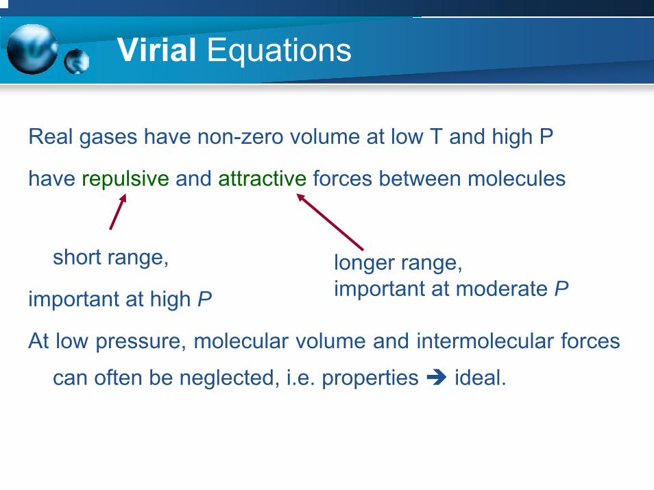
Real gases have non-zero volume at low T and high P
have repulsive and attractive forces between molecules
short range,
important at high P
At low pressure, molecular volume and intermolecular forces
can often be neglected, i.e. properties ideal.
longer range,important at moderate P
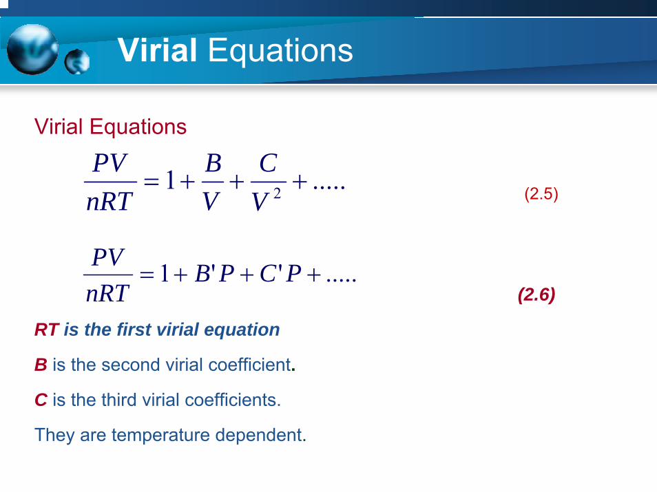
Virial Equations
Virial Equations
(2.5)
(2.6)
RT is the first virial equation
B is the second virial coefficient.
C is the third virial coefficients.
They are temperature dependent.
.....1 2 +++=VC
VB
nRTPV
.....''1 +++= PCPBnRTPV
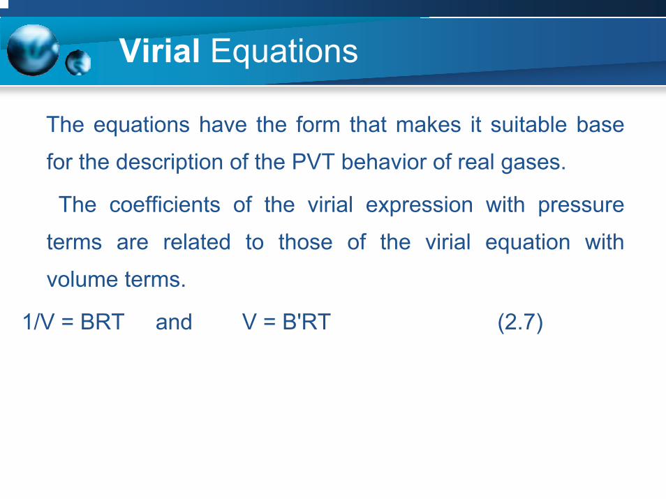
Virial Equations
The equations have the form that makes it suitable base
for the description of the PVT behavior of real gases.
The coefficients of the virial expression with pressure
terms are related to those of the virial equation with
volume terms.
1/V = BRT and V = B'RT (2.7)
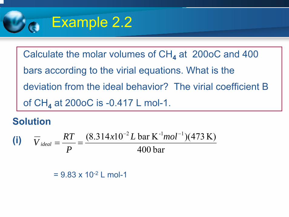
Example 2.2
Calculate the molar volumes of CH4 at 200oC and 400
bars according to the virial equations. What is the
deviation from the ideal behavior? The virial coefficient B
of CH4 at 200oC is -0.417 L mol-1.
Solution
(i)bar 400
K) 473)(Kbar 10314.8( 1-12 −−
==molLx
PRTV ideal
= 9.83 x 10⁻² L mol-1
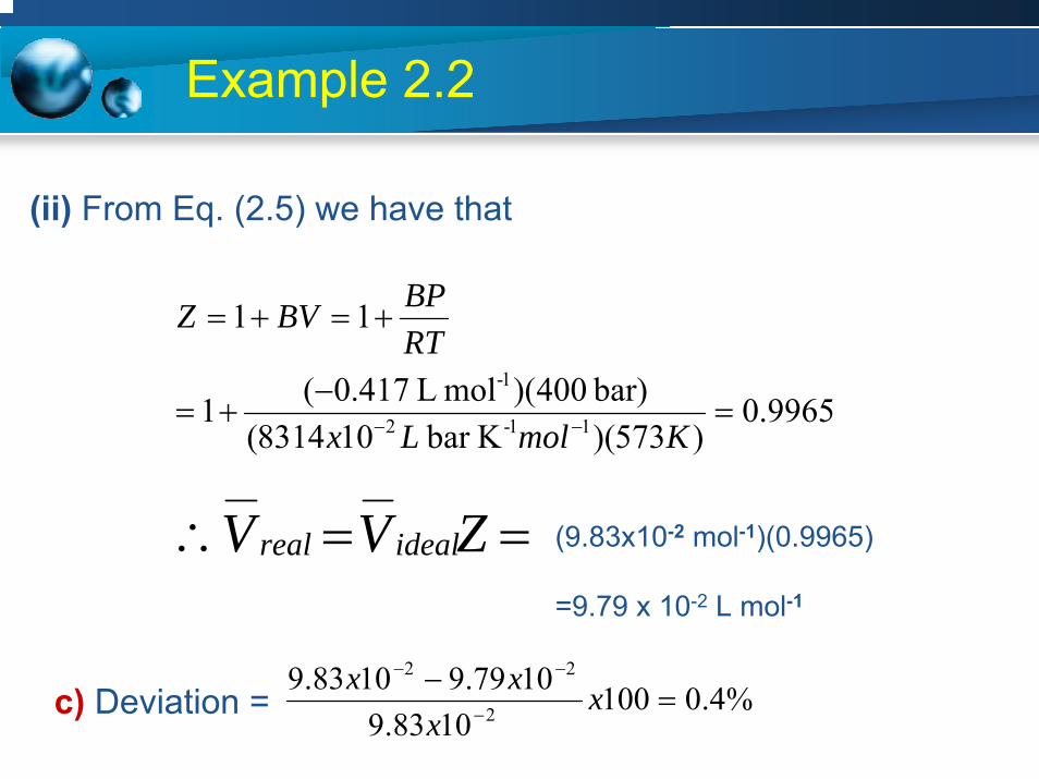
Example 2.2
(ii) From Eq. (2.5) we have that
9965.0)573)(Kbar 108314(
bar) 400)(mol L 417.0(1
11
11-2
1-
=−
+=
+=+=
−− KmolLx
RTBPBVZ
c) Deviation =
(9.83x10⁻² mol-1)(0.9965)
=9.79 x 10⁻² L mol-1
==∴ ZVV idealreal
%4.01001083.9
1079.91083.92
22
=−
−
−−
xx
xx
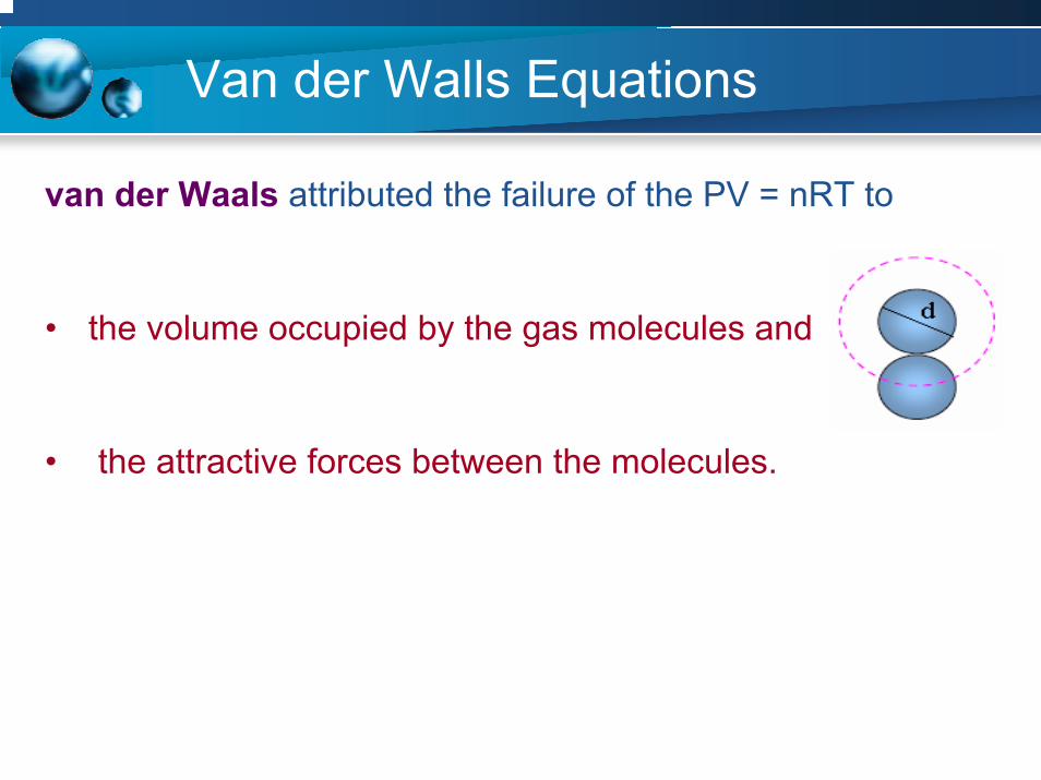
Van der Walls Equations
van der Waals attributed the failure of the PV = nRT to
• the volume occupied by the gas molecules and
• the attractive forces between the molecules.
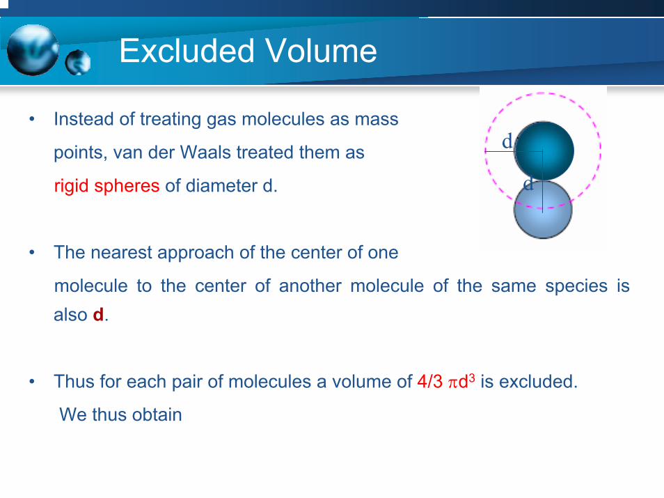
Excluded Volume
• Instead of treating gas molecules as mass
points, van der Waals treated them as
rigid spheres of diameter d.
• The nearest approach of the center of one
molecule to the center of another molecule of the same species is also d.
• Thus for each pair of molecules a volume of 4/3 πd3 is excluded.
We thus obtain
d
d

Excluded Volume
Thus we obtain that
Excluded volume per a molecule = Vexc
Vexc= ½ (4/3 πd3) = 4[1/8(4/3 πd3)] = 4[4/3 π(d/2)3]
The expression in brackets is the volume of a molecule.
Vexc= 4 times the actual volume of a molecule
Excluded volume for NA molecules = 4 times the actual volume of NA
molecules
Excluded Volume
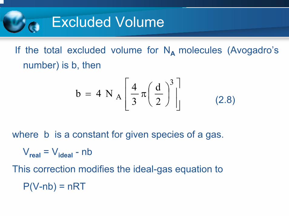
If the total excluded volume for NA molecules (Avogadro’s number) is b, then
(2.8)
where b is a constant for given species of a gas.
Vreal = Videal - nb
This correction modifies the ideal-gas equation to
P(V-nb) = nRT
⎥⎥⎦
⎤
⎢⎢⎣
⎡⎟⎠⎞
⎜⎝⎛π=
3
A 2d
34N 4b

Molecular Attraction
Van der Waals made the correction for attractive forces as follows.
• Attraction occurs between pairs of molecules,
• Molecular attraction decreases the number of collisions on the walls of
the container ( n/V )
• Attraction forces increases as the number of molecules increases in
the container (n/V )
• Attraction forces should proportional with
the square of the concentration of molecules, (n/v)2.
• Attractive forces = a(n/V)2
Molecular Attraction
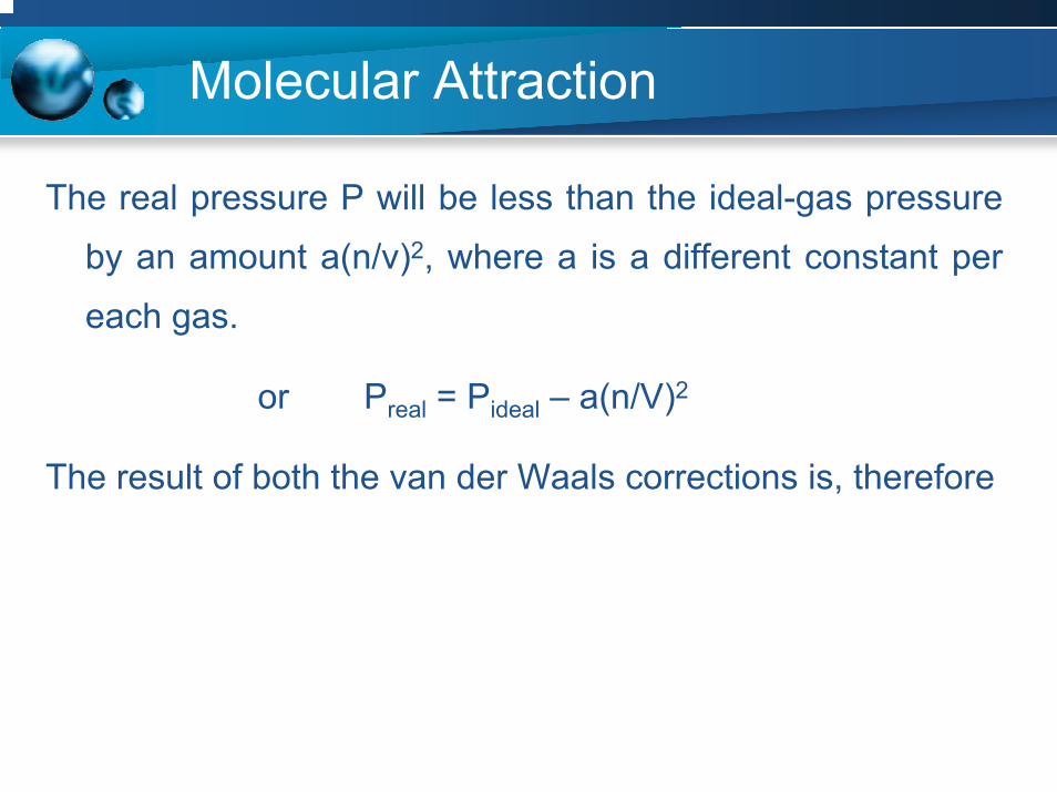
The real pressure P will be less than the ideal-gas pressure
by an amount a(n/v)2, where a is a different constant per
each gas.
or Preal = Pideal – a(n/V)2
The result of both the van der Waals corrections is, therefore
Molecular Attraction
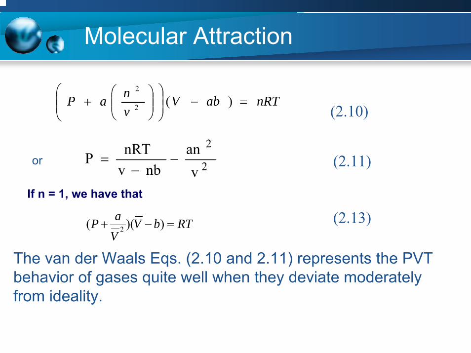
nRTabVvnaP =−⎟⎟
⎠
⎞⎜⎜⎝
⎛⎟⎟⎠
⎞⎜⎜⎝
⎛+ )(2
2
(2.10)
2
2
van
nbvnRTP −−
= (2.11)
(2.13)
The van der Waals Eqs. (2.10 and 2.11) represents the PVT behavior of gases quite well when they deviate moderately from ideality.
RTbVVaP =−+ ))(( 2
If n = 1, we have that
or
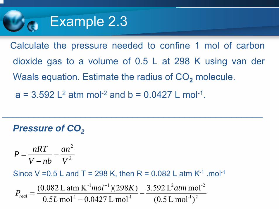
Example 2.3Calculate the pressure needed to confine 1 mol of carbon
dioxide gas to a volume of 0.5 L at 298 K using van der
Waals equation. Estimate the radius of CO2 molecule.
a = 3.592 L2 atm mol-2 and b = 0.0427 L mol-1.
__________________________________________________
Pressure of CO2
2
2
Van
nbVnRTP −−
=
Since V =0.5 L and T = 298 K, then R = 0.082 L atm K-1 .mol-1
21-
-22
1-1-
1-1
)mol L 5.0(mol L 592.3
mol L 0427.0mol 5.0)298)(K atm L 082.0( atm
LKmolPreal −
−=
−
Example 2.3
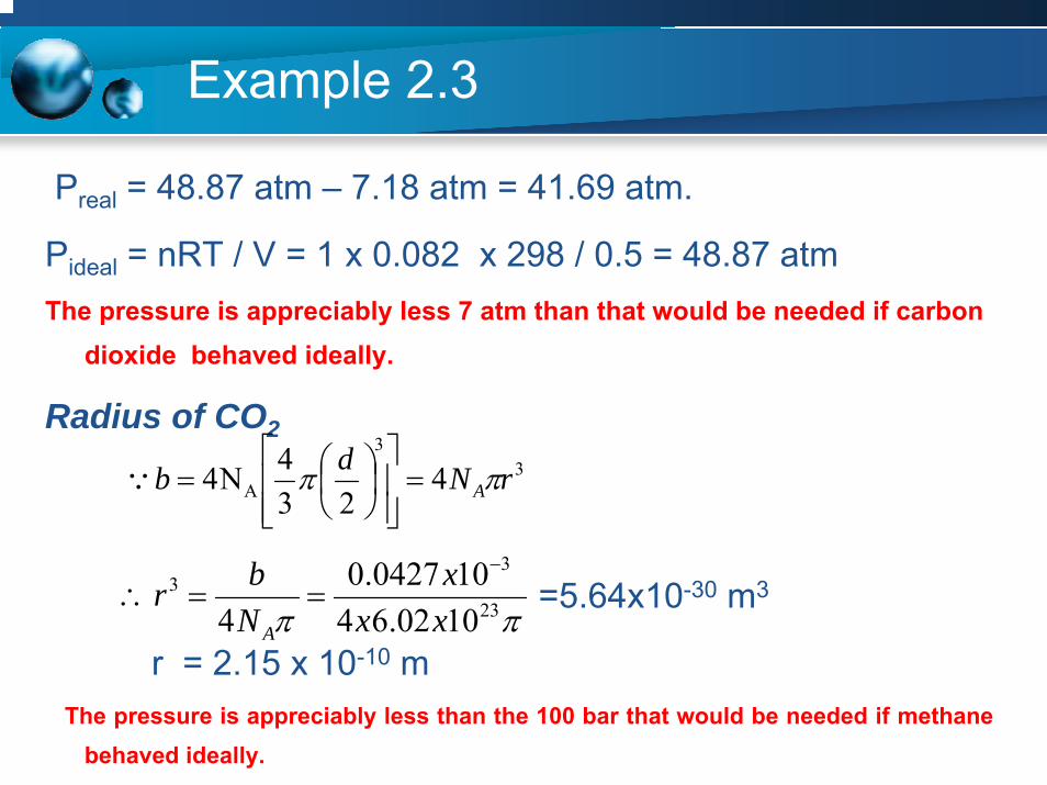
Preal = 48.87 atm – 7.18 atm = 41.69 atm.
Pideal = nRT / V = 1 x 0.082 x 298 / 0.5 = 48.87 atmThe pressure is appreciably less 7 atm than that would be needed if carbon
dioxide behaved ideally.
Radius of CO2
=5.64x10⁻³⁰ m3
r = 2.15 x 10⁻¹⁰ mThe pressure is appreciably less than the 100 bar that would be needed if methane
behaved ideally.
33
A 423
4N4 rNdb Aππ =⎥⎥⎦
⎤
⎢⎢⎣
⎡⎟⎠⎞
⎜⎝⎛=Q
ππ 23
33
1002.64100427.0
4 xxx
Nbr
A
−
==∴
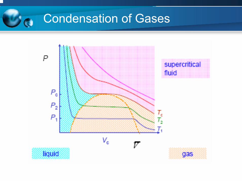
Condensation of Gases
The constants of van der Waals equation can be evaluated from critical-point data.
• Tc is the critical temperature which is defined as the highest temperature at which liquid and vapor can exist together (condensation of the gas is possible) .
• Pc is the pressure at which condensation of vapor to liquid occurs when the temperature is equal to Tc or the highest pressure at which liquid will boil when heated.
• Vc is the volume of a mol of the substance at Tc and Pc
The constants of van der Waals equation can be evaluated from critical-point data.
Tc, Pc and Vc are the critical constants of the gas.
Above the critical temperature the gas and liquid
phases are continuous, i.e. there is no interface.
Van der Waals equation, or any of the other two-
parameter equations of Table 2.1, cannot describe
the detained PV behavior of a gas in the region of
liquid-vapor equilibrium.
The constants of van der Waals equation can be evaluated from critical-point data.
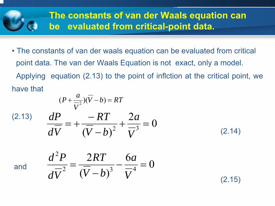
• The constants of van der waals equation can be evaluated from critical point data. The van der Waals Equation is not exact, only a model.
Applying equation (2.13) to the point of inflction at the critical point, we
have that
(2.13)
(2.14)
and
(2.15)
RTbVVaP =−+ ))(( 2
02)( 32 =+
−−
+=V
abV
RTVd
dP
06)(
2432
2
=−−
=V
abV
RTVdPd
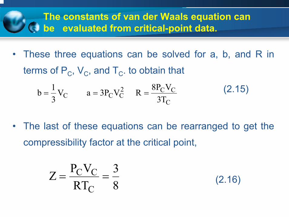
The constants of van der Waals equation can be evaluated from critical-point data.
• These three equations can be solved for a, b, and R in
terms of PC, VC, and TC. to obtain that
(2.15)
• The last of these equations can be rearranged to get the
compressibility factor at the critical point,
(2.16)
C
CC2CCC T3
VP8RVP3aV31b ===
83
RTVPZ
C
CC ==

The constants of van der Waals equation can be evaluated from critical-point data.
The values of a and b are often chosen so that the van der
Waals PV isotherm with a horizontal point of inflection
occurs at PC and TC.
This procedure can be followed by eliminating the VC term,
by using VC = 3b, from the other expression of Eq. (2.15).
The resulting expressions for a and b are
(2.17)C
CC
PRTbandTa8P 64
R 27
C
22
==

The constants of van der Waals equation can be evaluated from critical-point data.
Gas
H2 0.33
He 0.32
CH4 0.29
NH3 0.24
N2 0.29
O2 0.29
C
CC
RTVP

Example 2.5
Evaluate the van der Waals constants for O2 using
TC = -118.40C and PC = 50.1 atm.
________________________________________________
Using Eq. (2.17) gives that
2-2221-122
mol 360.1atm) 1.50(64
K) 8.154()K atm L )082.0(2764
27 atmLmolPTRaC
C ===−
2-222-1-1
C
C mol atmL 0317.0atm) 1.50(8
K) 8.154()mol K atm L 082.0(P8
RTb ===
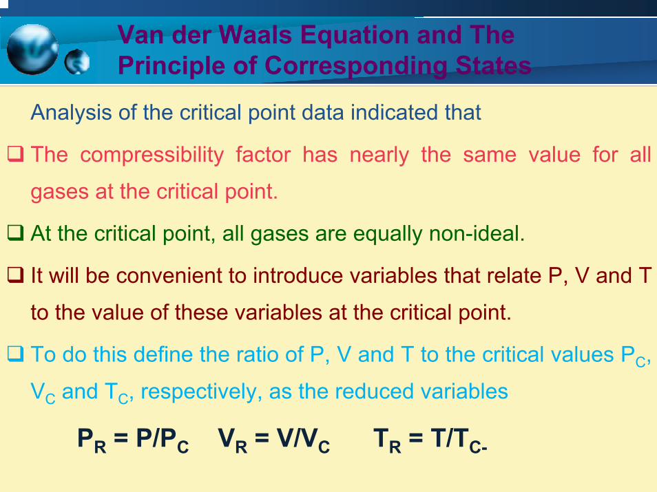
Van der Waals Equation and The Principle of Corresponding States
Analysis of the critical point data indicated that
The compressibility factor has nearly the same value for all
gases at the critical point.
At the critical point, all gases are equally non-ideal.
It will be convenient to introduce variables that relate P, V and T
to the value of these variables at the critical point.
To do this define the ratio of P, V and T to the critical values PC,
VC and TC, respectively, as the reduced variables
PR = P/PC VR = V/VC TR = T/TC-

Van der Waals Equation and The Principle of Corresponding States
J.H. Van der Waals pointed out
that, to fairly good approximation
at moderate pressures, all gases
follow the same equation of state
in terms of reduced variables.
He called this rule the principle of corresponding states.
This behavior is illustrated for a
number of different gases.
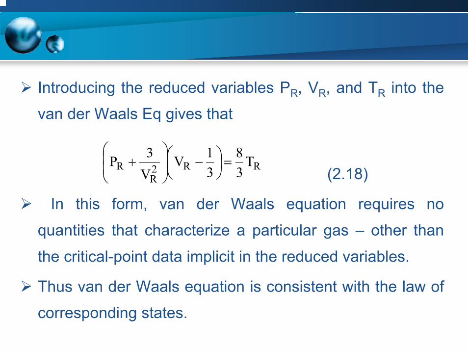
Introducing the reduced variables PR, VR, and TR into the
van der Waals Eq gives that
(2.18)
In this form, van der Waals equation requires no
quantities that characterize a particular gas – other than
the critical-point data implicit in the reduced variables.
Thus van der Waals equation is consistent with the law of
corresponding states.
RR2R
R T38
31V
V3P =⎟
⎠⎞
⎜⎝⎛ −⎟⎟⎠
⎞⎜⎜⎝
⎛+
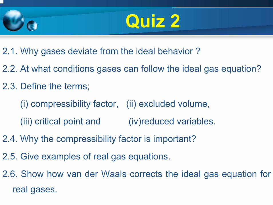
Quiz 22.1. Why gases deviate from the ideal behavior ?
2.2. At what conditions gases can follow the ideal gas equation?
2.3. Define the terms;
(i) compressibility factor, (ii) excluded volume,
(iii) critical point and (iv)reduced variables.
2.4. Why the compressibility factor is important?
2.5. Give examples of real gas equations.
2.6. Show how van der Waals corrects the ideal gas equation for
real gases.

Theory of Gases
Kinetic Theory of GasesKinetic Theory of Gases
Equations of Real GasesEquations of Real Gases
Distribution of Velocities of Gas Molecules Distribution of Velocities of Gas Molecules
Speeds of Gas Molecules Speeds of Gas Molecules
Molecular Collision
Transport Phenomena In Gases
Molecular Collision
Transport Phenomena In Gases
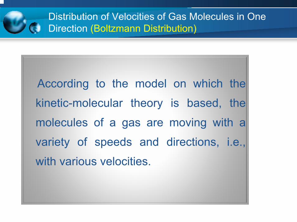
Distribution of Velocities of Gas Molecules in One Direction (Boltzmann Distribution)
According to the model on which the
kinetic-molecular theory is based, the
molecules of a gas are moving with a
variety of speeds and directions, i.e.,
with various velocities.
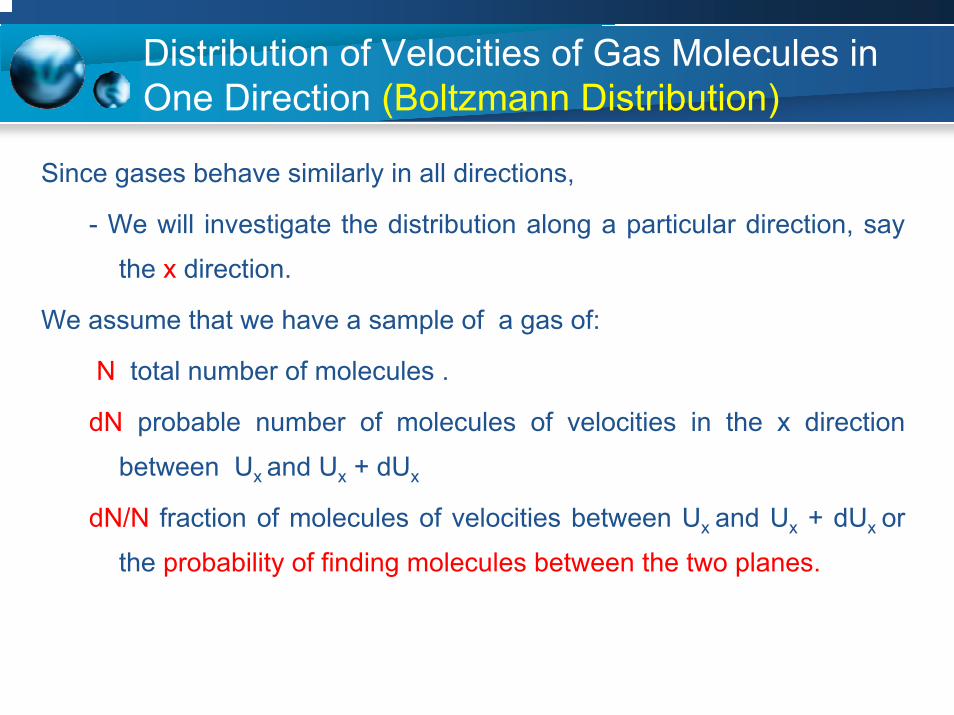
Distribution of Velocities of Gas Molecules in One Direction (Boltzmann Distribution)
Since gases behave similarly in all directions,
- We will investigate the distribution along a particular direction, say
the x direction.
We assume that we have a sample of a gas of:
N total number of molecules .
dN probable number of molecules of velocities in the x direction
between Ux and Ux + dUx
dN/N fraction of molecules of velocities between Ux and Ux + dUx or
the probability of finding molecules between the two planes.

Distribution of Velocities of Gas Molecules in One Direction (Boltzmann Distribution)
This is also the probability of finding molecules with velocity components between two planes

Distribution of Velocities of Gas Molecules in One Direction (Boltzmann Distribution)
The probability is expressed also as f(ux) dux component .
For each molecule ε = ½ mUx2
According to the Boltzmann distribution expression,
This constant can be evaluated by recognizing that integration of the right side of Eq. (3.1) over all possible values of ux, that is, from ux = -∞ to ux = +∞, must account for all the velocity points. Thus we can write
xkTmu due
NdN
x /)2/1( 2−α xkTmu duAe
NdN
x /)2/1( 2−=∴ (3.1)
∫+∞
∞−
− = 1du x/)2/1( 2 kTmu xeA (3.2)
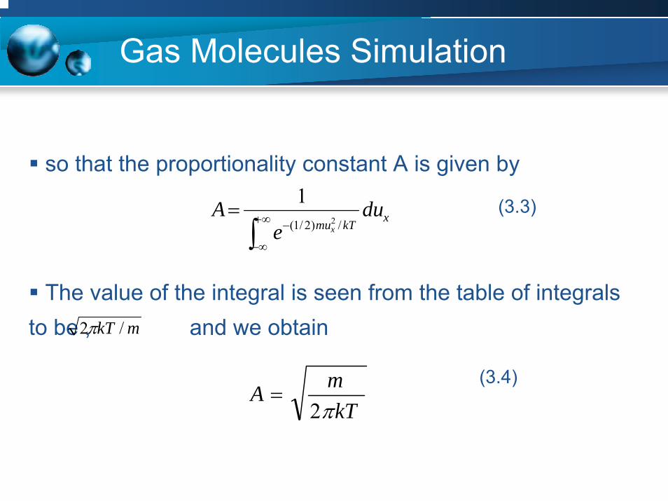
Gas Molecules Simulation
so that the proportionality constant A is given by
(3.3)
The value of the integral is seen from the table of integrals to be , and we obtain
(3.4)
xkTmudu
eA
x∫∞+
∞−
−=
/)2/1( 2
1
kTmAπ2
=
mkT /2π
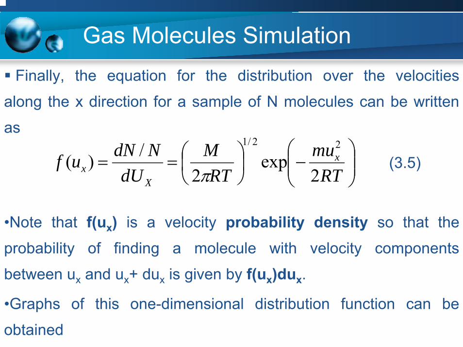
Gas Molecules SimulationFinally, the equation for the distribution over the velocities
along the x direction for a sample of N molecules can be written
as
(3.5)
•Note that f(ux) is a velocity probability density so that the
probability of finding a molecule with velocity components
between ux and ux+ dux is given by f(ux)dux.
•Graphs of this one-dimensional distribution function can be
obtained
⎟⎟⎠
⎞⎜⎜⎝
⎛−⎟
⎠⎞
⎜⎝⎛==
RTmu
RTM
dUNdNuf x
Xx 2
exp2
/)(22/1
π
Gas Molecules Simulation
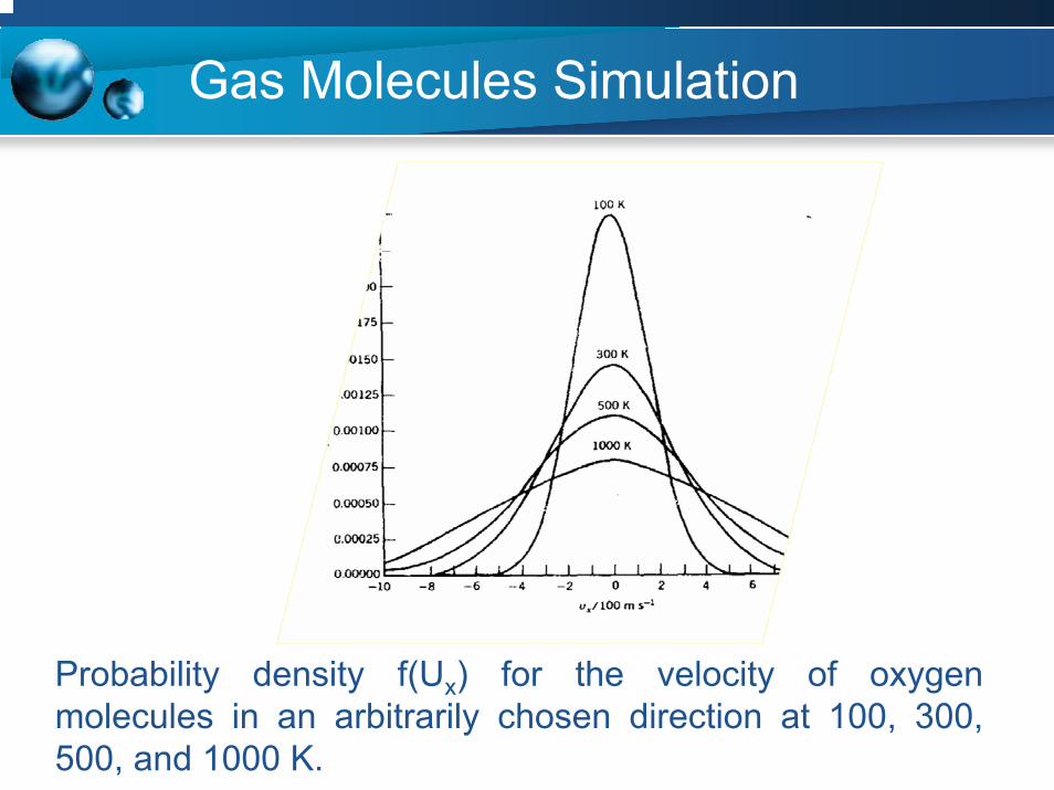
Probability density f(Ux) for the velocity of oxygen molecules in an arbitrarily chosen direction at 100, 300, 500, and 1000 K.

Example 3.1
Calculate the probability density for ux of N2 molecules at 300 K.
__________________________________________________
Using equation (3.5)
= 8.065 x 10⁻⁴ s m-1
⎟⎟⎠
⎞⎜⎜⎝
⎛−⎟
⎠⎞
⎜⎝⎛π
=RT2
muexpRT2
M)u(f2x
2/1
x
⎥⎦
⎤⎢⎣
⎡−⎥
⎦
⎤⎢⎣
⎡= −−
−
−− )300)(314.8(2)300)(mol 028.0(exp
)300)(314.8(2ol028.0
11
211-2/1
11
1-
KmolJKmsg
KmolJKgm
π
ExerciseCalculate the probability density of N2 at 0 and 600 K.

Maxwell – Boltzmann Distribution(in three dimensions)
The speed u of a molecule is related its component velocities by
(3.6)
Therefore, F(u) du is the probability of finding a molecule with a speed
between u and u + du .
The one-dimensional distribution can be combined to give the fraction of
the molecules that have velocity components between ux and ux+dux, ux
and u y+ duy and uz and uz + duz.
2z
2y
2x
2 uuuu ++=

Maxwell – Boltzmann Distribution(in three dimensions)
It is given analytically ;
f(ux, uy, uz) duxduy,duz =
(3.7)
The probability of finding a molecule with velocity
components between u and u+ du is given by
(3.8)
NdN
( ) zyxzyx dududuuuukTm
kTm
NdN
⎥⎦⎤
⎢⎣⎡ ++−⎟
⎠⎞
⎜⎝⎛=∴ 222
2/3
2exp
2π
dukT
mukT
muduuF ⎟⎟⎠
⎞⎜⎜⎝
⎛⎟⎠⎞
⎜⎝⎛=
2exp
24)(
22/32
ππ
Maxwell – Boltzmann Distribution(in three dimensions)
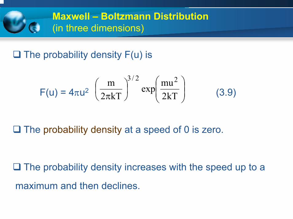
The probability density F(u) is
F(u) = 4πu2 (3.9)
The probability density at a speed of 0 is zero.
The probability density increases with the speed up to a
maximum and then declines.
⎟⎟⎠
⎞⎜⎜⎝
⎛⎟⎠⎞
⎜⎝⎛
π kT2muexp
kT2m 22/3
Maxwell – Boltzmann Distribution(in three dimensions)
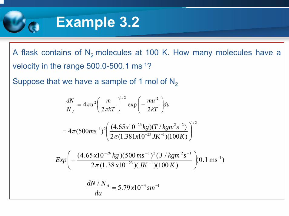
Example 3.2
A flask contains of N2 molecules at 100 K. How many molecules have a
velocity in the range 500.0-500.1 ms-1?
Suppose that we have a sample of 1 mol of N2
dukT
mukT
muNdN
A⎟⎟⎠
⎞⎜⎜⎝
⎛−⎟
⎠⎞
⎜⎝⎛=
2exp
24
22/12
ππ
2/1
123
222621
)100)(10381.1(2)/)(1065.4()500(4 ⎟⎟⎠
⎞⎜⎜⎝
⎛= −−
−−−
KJKxskgmTkgxms
ππ
)ms 1.0()100)()(1038.1(2
/()500)(1065.4( 1-123
122126
⎟⎟⎠
⎞⎜⎜⎝
⎛− −−
−−−
KJKxskgmJmskgxExp
π
141079.5/ −−= smxdu
NdN A
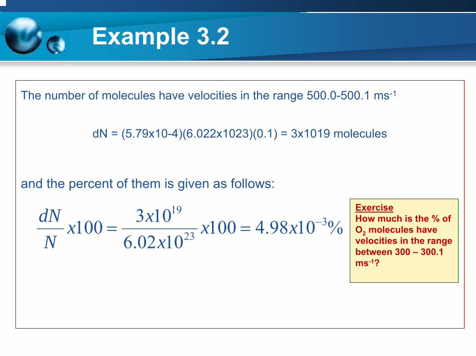
Example 3.2
The number of molecules have velocities in the range 500.0-500.1 ms-1
dN = (5.79x10⁻⁴)(6.022x10²³)(0.1) = 3x10¹⁹ molecules
and the percent of them is given as follows:
%1098.41001002.6
103100 323
19−== xx
xxx
NdN Exercise
How much is the % of O2 molecules have velocities in the range between 300 – 300.1 ms-1?
Theory of Gases
Kinetic Theory of GasesKinetic Theory of Gases
Equations of Real GasesEquations of Real Gases
Distribution of Velocities of Gas Molecules Distribution of Velocities of Gas Molecules
Speeds of Gas Molecules Speeds of Gas Molecules
Molecular Collision
Transport Phenomena In Gases
Molecular Collision
Transport Phenomena In Gases

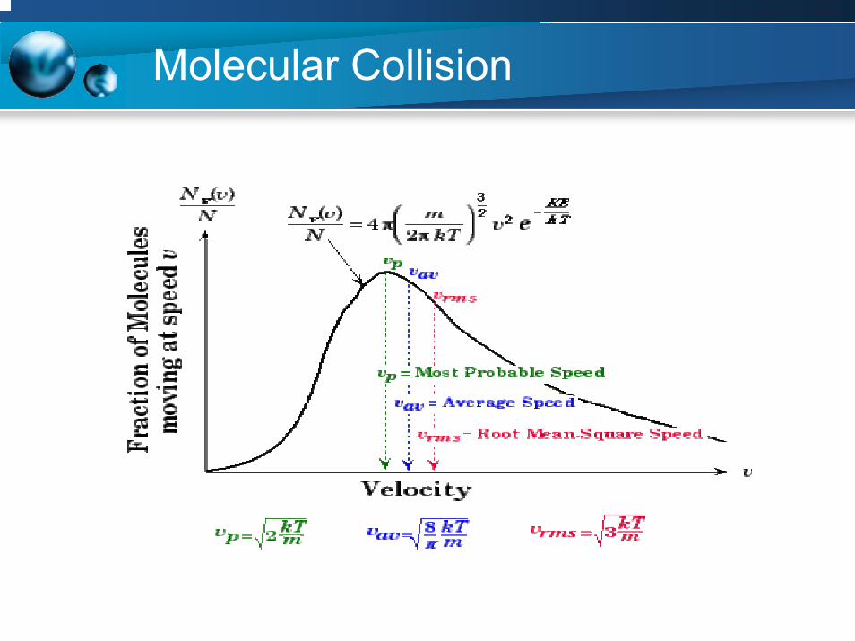
Speeds of Gas Molecules
The speed of gas molecules is of three types
• Most Probable Speed (up )
• Mean (average) Speed (ū)
• Root mean-square Speed (urms).
Speeds of Gas Molecules
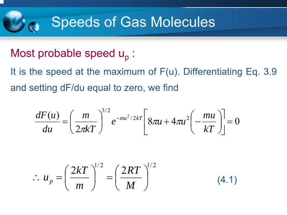
It is the speed at the maximum of F(u). Differentiating Eq. 3.9
and setting dF/du equal to zero, we find
(4.1)
0482
)( 22/2/3
2
=⎥⎦
⎤⎢⎣
⎡⎟⎠⎞
⎜⎝⎛−+⎟
⎠⎞
⎜⎝⎛= −
kTmuuue
kTm
duudF kTmu ππ
π
Most probable speed up :
2/12/1 22⎟⎠⎞
⎜⎝⎛=⎟
⎠⎞
⎜⎝⎛=∴
MRT
mkTup
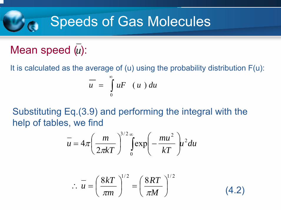
Speeds of Gas Molecules
It is calculated as the average of (u) using the probability distribution F(u):
∫∞
=0
)( duuuFu
Mean speed ( ):
Substituting Eq.(3.9) and performing the integral with the help of tables, we find
(4.2)
∫∞
⎟⎟⎠
⎞⎜⎜⎝
⎛−⎟
⎠⎞
⎜⎝⎛=
0
222/3
exp2
4 duukT
mukT
muπ
π
2/12/1 88⎟⎠⎞
⎜⎝⎛=⎟
⎠⎞
⎜⎝⎛=∴
MRT
mkTu
ππ
u

Speeds of Gas Molecules
Which is defined as the square root of
Substituting Eq. 3.9 and using tables again, we find
(4.3)
2/1
0
22/12 )()(⎥⎥
⎦
⎤
⎢⎢
⎣
⎡== ∫
∞
duuFuuurms
Root-mean square speed (urms):
2/12/1 33⎟⎠⎞
⎜⎝⎛=⎟
⎠⎞
⎜⎝⎛=
MRT
mkTurms
2u

Speeds of Gas Molecules
We can see that at any temperature
2/12/1 22⎟⎠⎞
⎜⎝⎛=⎟
⎠⎞
⎜⎝⎛=
MRT
mkTu p
From these three calculations,
2/12/1 88⎟⎠⎞
⎜⎝⎛=⎟
⎠⎞
⎜⎝⎛=
MRT
mkTu
ππ
2/12/1 33⎟⎠⎞
⎜⎝⎛=⎟
⎠⎞
⎜⎝⎛=
MRT
mkTurms
pu u >>rmsu
Molecular Collision

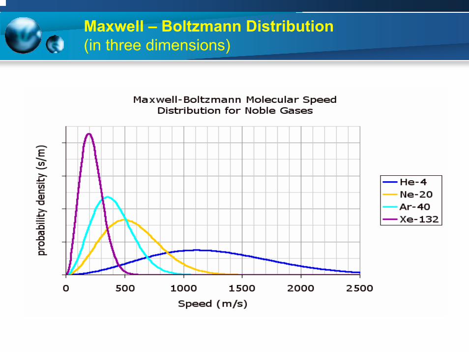
Speeds of Gas Molecules
Each of these speeds is proportional to (T/M)1/2 .
Each increases with temperature
Each decreases with molar mass. Lighter molecules therefore
move faster than heavier molecules on average, as shown in
the following table.
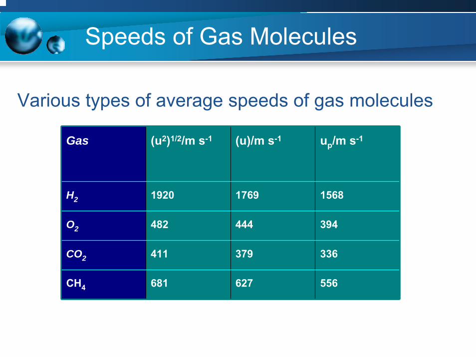
Speeds of Gas Molecules
Various types of average speeds of gas molecules
up/m s-1(u)/m s-1(u2)1/2/m s-1Gas
156817691920H2
394444482O2
336379411CO2
556627681CH4
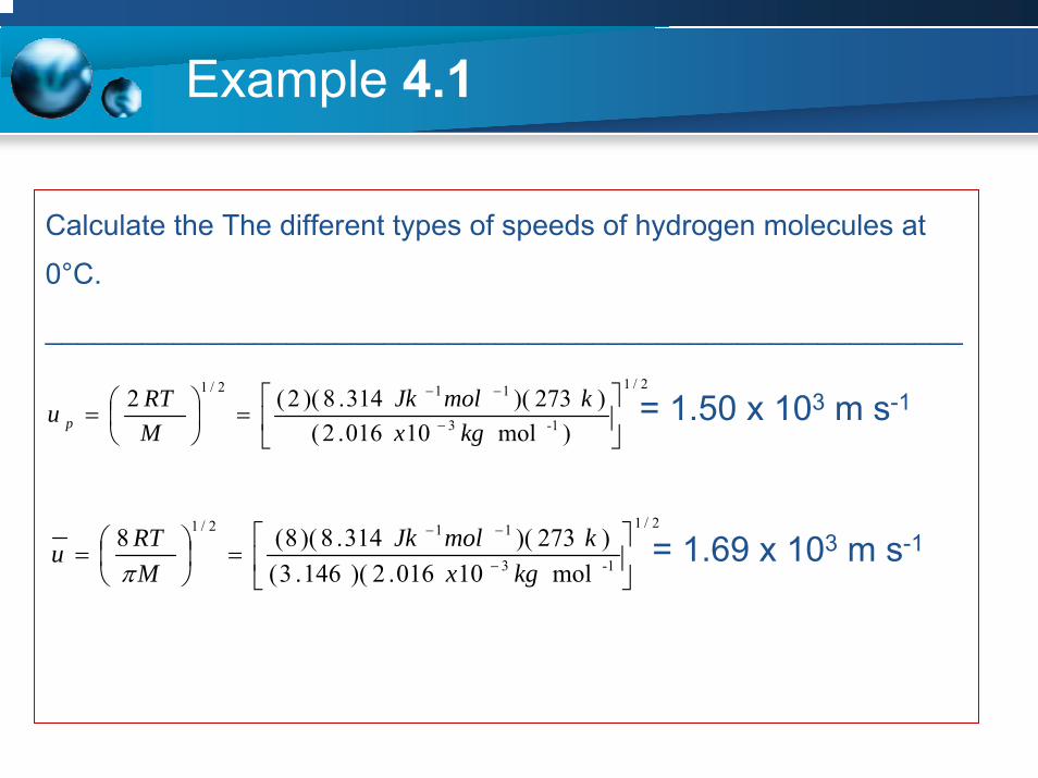
Example 4.1
Calculate the The different types of speeds of hydrogen molecules at
0°C.
_________________________________________________________
2/1
1-3
112/1
)mol 10016.2()273)(314.8)(2(2⎥⎦
⎤⎢⎣
⎡=⎟
⎠⎞
⎜⎝⎛= −
−−
kgxkmolJk
MRTu p
2/1
1-3
112/1
mol 10016.2)(146.3()273)(314.8)(8(8⎥⎦
⎤⎢⎣
⎡=⎟
⎠⎞
⎜⎝⎛= −
−−
kgxkmolJk
MRTuπ
= 1.50 x 10³ m s-1
= 1.69 x 10³ m s-1
Example 4.1
⎥⎦
⎤⎢⎣
⎡=⎟
⎠⎞
⎜⎝⎛= −
−−
1-3
2/1112/1
mol 1006.2)15.273)(314.8(33
kgxkmolJk
MRTurms
The root-mean square speed of a hydrogen molecule at 0°C is 6620 kmh-1, but at ordinary pressures it travels only an exceedingly short distance before colliding with another molecule and changing direction.
= 1.84 x 10³ m s-1
ExerciseHow many molecules have a velocity exactly equal to 500 ms-1?
ExerciseHow many molecules have a velocity exactly equal to 500 ms-1?

Theory of Gases
Kinetic Theory of GasesKinetic Theory of Gases
Equations of Real GasesEquations of Real Gases
Distribution of Velocities of Gas Molecules Distribution of Velocities of Gas Molecules
Speeds of Gas Molecules Speeds of Gas Molecules
Molecular Collision
Transport Phenomena In Gases
Molecular Collision
Transport Phenomena In Gases
Molecular Collision
COLLISION PROPERTIES
OF GAS MOLECULES

Molecular Collision
Two Gases
Mean Free PathOne Gas
COLLISION
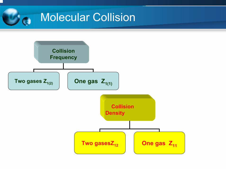
Molecular Collision
Collision Density
Two gasesZ12 One gas Z11
Collision Frequency
Two gases Z1(2) One gas Z1(1)
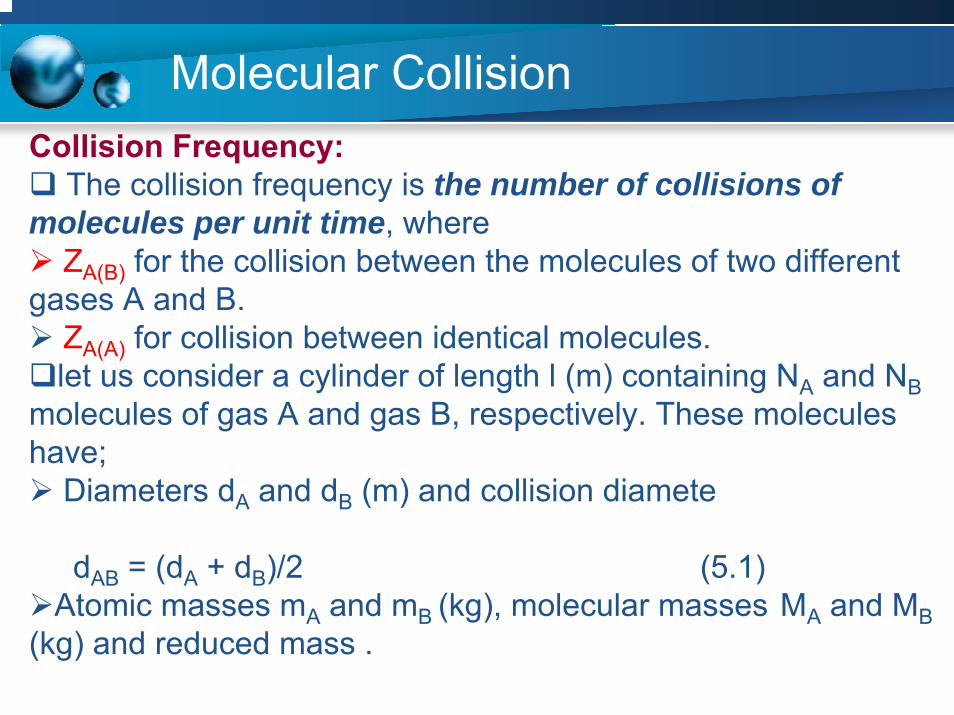
Molecular CollisionCollision Frequency:
The collision frequency is the number of collisions of molecules per unit time, where
ZA(B) for the collision between the molecules of two different gases A and B.
ZA(A) for collision between identical molecules.let us consider a cylinder of length l (m) containing NA and NB
molecules of gas A and gas B, respectively. These molecules have;
Diameters dA and dB (m) and collision diamete
dAB = (dA + dB)/2 (5.1)Atomic masses mA and mB (kg), molecular masses MA and MB
(kg) and reduced mass .
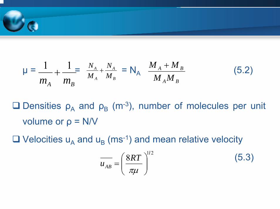
µ = = = NA (5.2)
Densities ρA and ρB (m-3), number of molecules per unit
volume or ρ = N/V
Velocities uA and uB (ms-1) and mean relative velocity
(5.3)
BA mm11
+B
A
A
A
MN
MN
+BA
BA
MMMM +
218
l
ABRTu ⎟⎟
⎠
⎞⎜⎜⎝
⎛=
πµ
Molecular Collision
Clickhere to
seeFlash
file
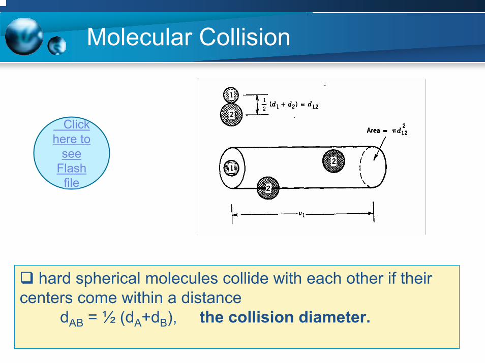
hard spherical molecules collide with each other if their centers come within a distance
dAB = ½ (dA+dB), the collision diameter.

Collision of different molecules
AAB ud 2π
Molecules of type B are stationary.
A molecule of type A will collide in unit time with all
molecules of type B that have their centers in a cylinder of
Volume =
A molecule of type A would undergo a
number of collisions =
per unit time.
BAABud ρπ 2
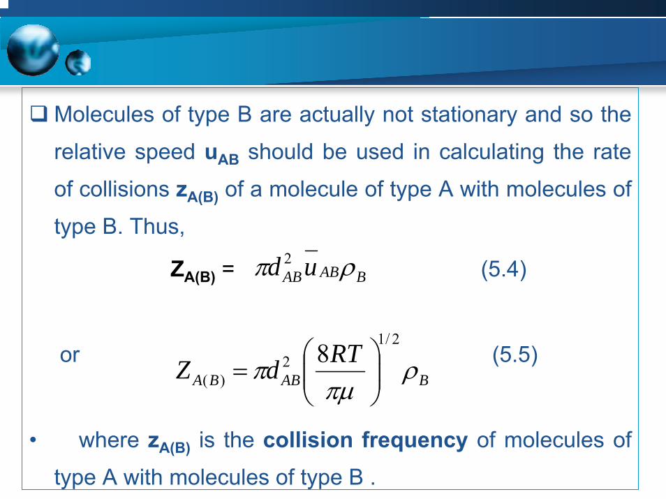
Molecules of type B are actually not stationary and so the
relative speed uAB should be used in calculating the rate
of collisions zA(B) of a molecule of type A with molecules of
type B. Thus,
ZA(B) = (5.4)
or (5.5)
• where zA(B) is the collision frequency of molecules of
type A with molecules of type B .
BABABud ρπ 2
BABBARTdZ ρπµ
π2/1
2)(
8⎟⎟⎠
⎞⎜⎜⎝
⎛=
Molecular Collision
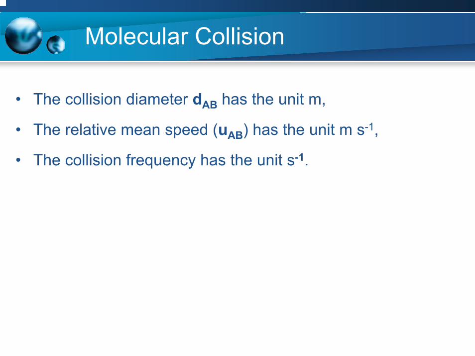
• The collision diameter dAB has the unit m,
• The relative mean speed (uAB) has the unit m s-1,
• The collision frequency has the unit s-1.

Collision Frequency of Identical Molecules
Now a molecule of type A is moving through molecules of
type A, rather than molecules of type B, Eq. (5.4)
becomes
(5.6)
Or (5.7)
AAAAA udZ ρπ 2)( =
BABBARTdZ ρπµ
π2/1
2)(
8⎟⎟⎠
⎞⎜⎜⎝
⎛=
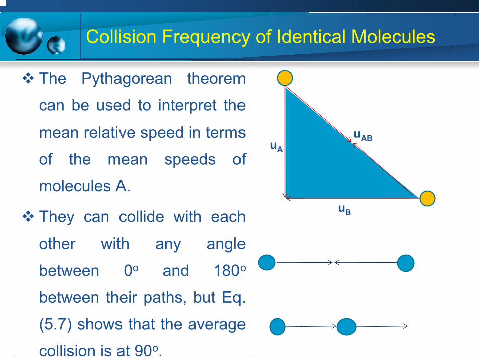
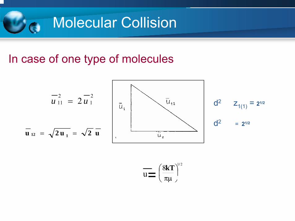
Collision Frequency of Identical Molecules
The Pythagorean theorem
can be used to interpret the
mean relative speed in terms
of the mean speeds of
molecules A.
They can collide with each
other with any angle
between 0o and 180o
between their paths, but Eq.
(5.7) shows that the average
collision is at 90o.
uABuA
uB
Molecular Collision
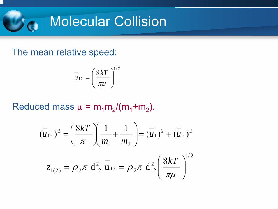
The mean relative speed:2/1
128
⎟⎟⎠
⎞⎜⎜⎝
⎛=
πµkTu
Reduced mass µ = m1m2/(m1+m2).
22
21
21
212 )()(118)( uu
mmkTu +=⎟⎟
⎠
⎞⎜⎜⎝
⎛+⎟
⎠⎞
⎜⎝⎛=π
2/1212212
2122)2(1
8d u d ⎟⎟⎠
⎞⎜⎜⎝
⎛==
πµπρπρ kTz
Molecular Collision
In case of one type of molecules
u 2u2u 112 ==
21
211 2 uu = z1(1) = 21/2��d2
= 21/2��d2
218 /kT⎟⎠⎞
⎜⎝⎛πµu=

Molecular Collision
The collision frequency z1(1) is thus ,
* The rate of collisions of a molecule of a gas with moleculesof the same gas.
* The number of collision of one molecule of a gas with molecules of the same gas per unit time per unit volume

Example 3.1
What is the mean relative speed of H2 molecules with respect
to O2molecules (or oxygen molecules with respect to hydrogen
molecules) at 298 ?

Example 3.1
The molecular masses are:
kg10x348.3mol10x022.6
mol kg10x016.2m 271-23
-131
−−
==
kg10x314.5mol 10x022.6
mol kg10x00.32m 261-23
-132
−−
==
271126127 10x150.3])kg10x314.5(0kg10x348.3[( −−−−−− =+=µ
1-17
1232/1
12 s 1824)10150.3(
)298)(10381.1(88 mkgx
kJkxkTu =⎥⎦
⎤⎢⎣
⎡=⎟⎟
⎠
⎞⎜⎜⎝
⎛= −
−−
ππµ

Example 3.1
Note that the mean relative speed is closer to the mean speed
of molecular hydrogen (1920 ms-1) than to that of molecular
oxygen (482 ms-1) .
Collision Density
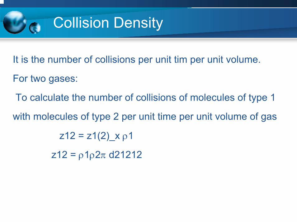
It is the number of collisions per unit tim per unit volume.
For two gases:
To calculate the number of collisions of molecules of type 1
with molecules of type 2 per unit time per unit volume of gas
z12 = z1(2)_x ρ1
z12 = ρ1ρ2π d21212
Collision Density
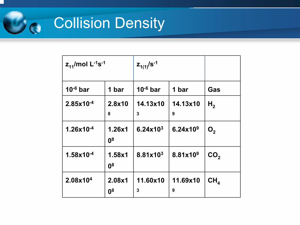
z11/mol L-1s-1 z1(1)/s-1
10-6 bar 1 bar 10-6 bar 1 bar Gas
2.85x10⁻⁴ 2.8x10⁸
14.13x10³
14.13x10⁹
H2
1.26x10⁻⁴ 1.26x10⁸
6.24x10³ 6.24x10⁹ O2
1.58x10⁻⁴ 1.58x10⁸
8.81x10³ 8.81x10⁹ CO2
2.08x10⁴ 2.08x10⁸
11.60x10³
11.69x10⁹
CH4
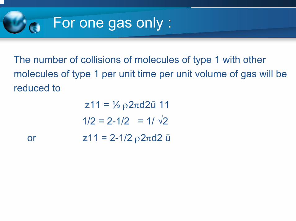
For one gas only :
The number of collisions of molecules of type 1 with other molecules of type 1 per unit time per unit volume of gas will bereduced to
z11 = ½ ρ2πd2ū 11 1/2 = 2-1/2 = 1/ √2
or z11 = 2-1/2 ρ2πd2 ū
For one gas only :
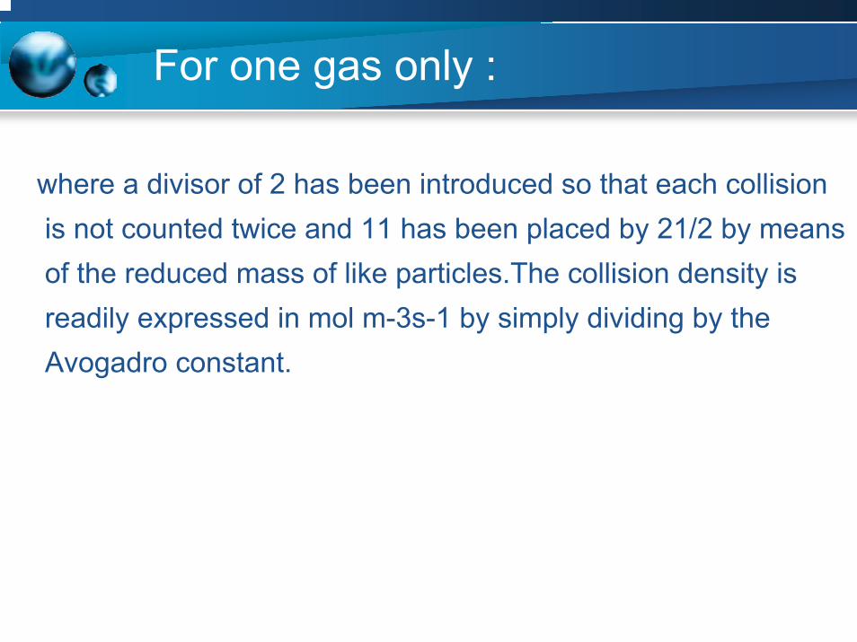
where a divisor of 2 has been introduced so that each collisionis not counted twice and 11 has been placed by 21/2 by meansof the reduced mass of like particles.The collision density isreadily expressed in mol m-3s-1 by simply dividing by theAvogadro constant.

For one gas only :
where a divisor of 2 has been introduced so that each
collision is not counted twice and 11 has been replaced by
21/2 by means of the reduced mass of like particles. The
collision density is readily expressed in mol m-3 s-1 by simply
dividing by the Avogadro constant.
For one gas only :
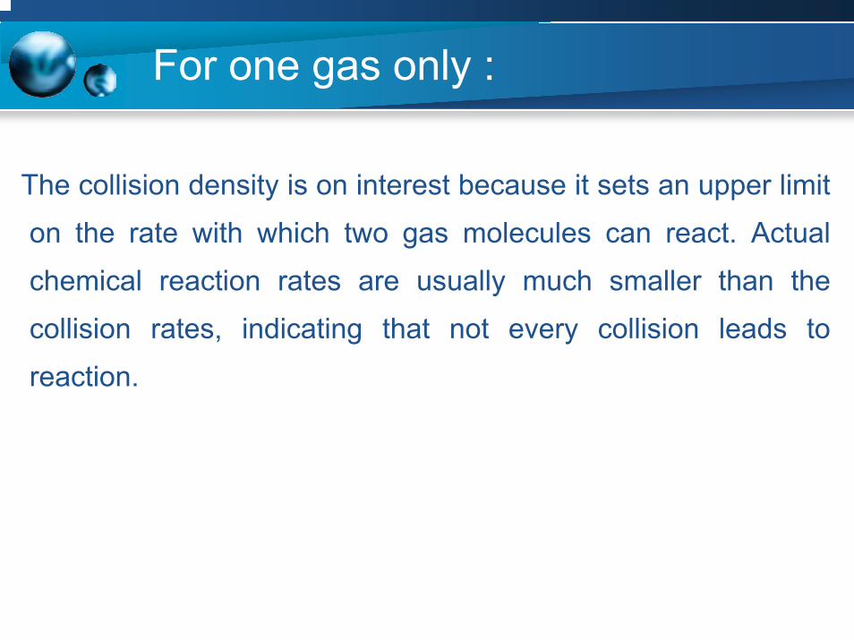
The collision density is on interest because it sets an upper limit
on the rate with which two gas molecules can react. Actual
chemical reaction rates are usually much smaller than the
collision rates, indicating that not every collision leads to
reaction.

For one gas only :
Collision frequencies z1(1) and collision densities z11 for four
gases are given in Table 3.1 at 25oC. The collision densities
are expressed in mol L-1 s-1 because it is easier to think about
chemical reactions in these units.
Example 3.2
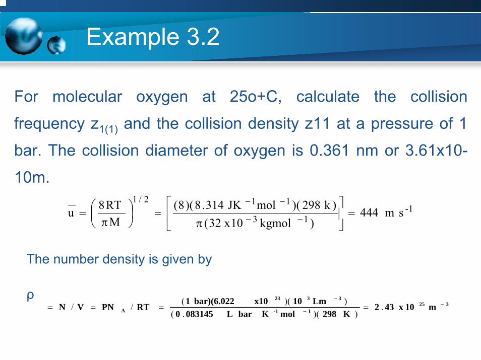
For molecular oxygen at 25o+C, calculate the collision
frequency z1(1) and the collision density z11 at a pressure of 1
bar. The collision diameter of oxygen is 0.361 nm or 3.61x10-
10m.
1-13
112/1s m 444
)kgmol10x32()k298)(molJK314.8)(8(
MRT8u =⎥
⎦
⎤⎢⎣
⎡
π=⎟
⎠⎞
⎜⎝⎛π
= −−
−−
The number density is given by
ρ325
1-1
3323
A m10x432K298molKbar L0831450
Lm10x10bar)(6.022 1RTPNVN −−
−
==== .))(.(
))((//
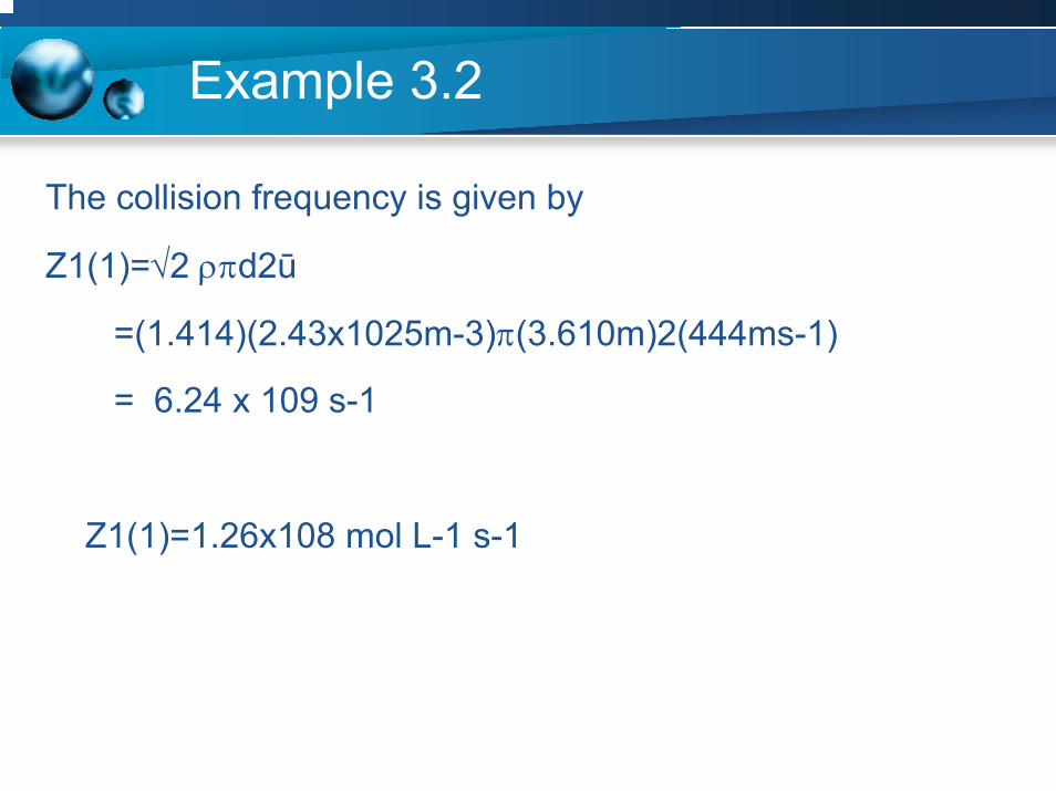
Example 3.2
The collision frequency is given by
Z1(1)=√2 ρπd2ū
=(1.414)(2.43x1025m-3)π(3.610m)2(444ms-1)
= 6.24 x 10⁹ s-1
Z1(1)=1.26x10⁸ mol L-1 s-1

Mean Free Path
• The mean free path λ is the average distance traveled between collisions.
• It can be computed by dividing the average distance traveled
per unit time by the collision frequency.
• For a molecule moving through like molecules.
22/1)1(1 d21
zu
ρπ==λ
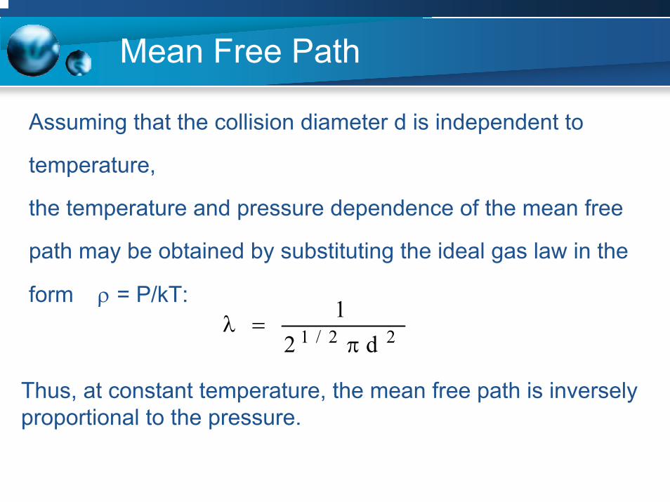
Mean Free Path
Assuming that the collision diameter d is independent to
temperature,
the temperature and pressure dependence of the mean free
path may be obtained by substituting the ideal gas law in the
form ρ = P/kT:
22/1 d21π
=λ
Thus, at constant temperature, the mean free path is inversely proportional to the pressure.
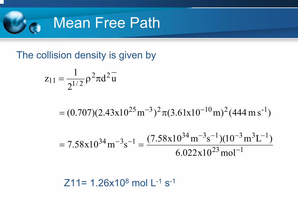
Mean Free Path
The collision density is given by
ud2
1z 222/111 πρ=
)s m 444()m10x61.3()m10x43.2)(707.0( -12102325 −− π=
123
13313341334
mol10x022.6)Lm10)(sm10x58.7(sm10x58.7 −
−−−−−− ==
Z11= 1.26x10⁸ mol L-1 s-1
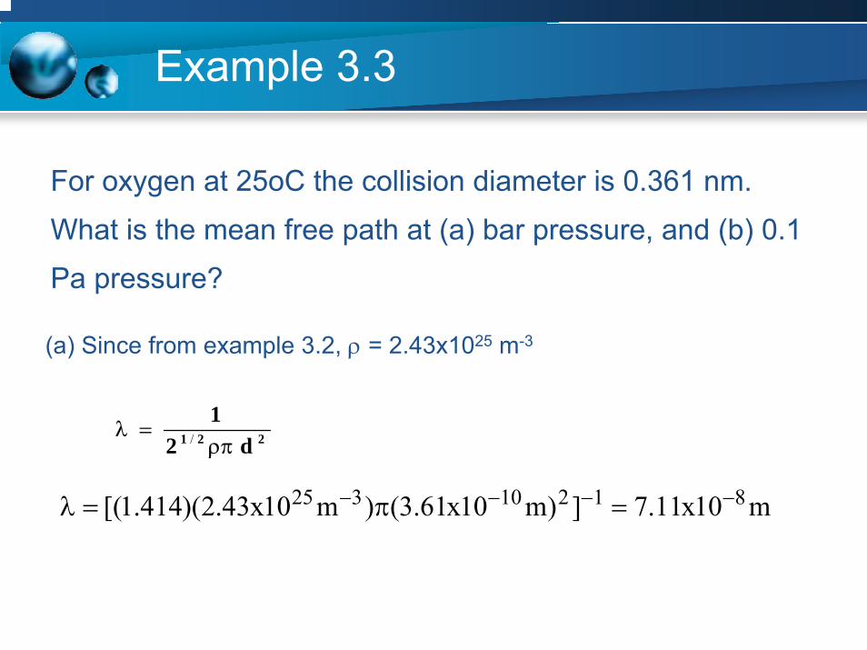
Example 3.3
For oxygen at 25oC the collision diameter is 0.361 nm.
What is the mean free path at (a) bar pressure, and (b) 0.1
Pa pressure?
(a) Since from example 3.2, ρ = 2.43x1025 m-3
221 d21ρπ
=λ /
m10x11.7])m10x61.3()m10x43.2)(414.1[( 81210325 −−−− =π=λ

Example 3.3
(b)
= 0.071 m = 7.1 cm
At pressure so low that the mean free path becomes
comparable with the dimensions of the containing vessel,
the flow properties of the gas become markedly different
from those at higher pressures.
3191-1
123A m10x432
K298molK J3148m10x0226Pa20
RTPN −
−
−
===ρ .))(.(
).)(.(
1319210 )]m10x43.3()m10x61.3)(14.3)(414.1[( −−−=λ

Theory of Gases
Kinetic Theory of GasesKinetic Theory of Gases
Equations of Real GasesEquations of Real Gases
Distribution of Velocities of Gas Molecules Distribution of Velocities of Gas Molecules
Speeds of Gas Molecules Speeds of Gas Molecules
Molecular Collision
Transport Phenomena In Gases
Molecular Collision
Transport Phenomena In Gases
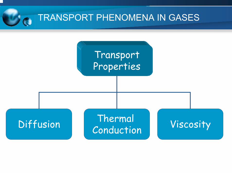
TRANSPORT PHENOMENA IN GASES
TransportProperties
Diffusion Thermal Conduction Viscosity

TRANSPORT PHENOMENA IN GASES
If a gas is not uniform with respect to• Composition• temperature, and • velocity,transport processes occur until the gas becomes uniform.Examples:
(1) Open a bottle of perfume at the front of a classroom:Good smell moves from front row to rear ( Diffusion).
(2) Metal bar, one end hot and one end cold:Heat flows from hot to cold end until temperaturebecomes (Thermal Conduction)
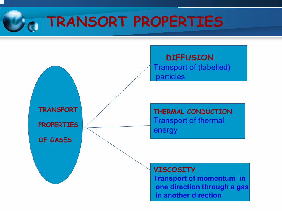
TRANSORT PROPERTIES
DIFFUSIONTransport of (labelled)particles
THERMAL CONDUCTIONTransport of thermal energy
VISCOSITYTransport of momentum inone direction through a gasin another direction
TRANSPORT
PROPERTIES
OF GASES

TRANSPORT PHENOMENA IN GASES
In each case,
Rate of flow ∞ Rate of change of some property with
distance, a so-called gradient
All have same mathematical form:
Flow of____(per unit area, unit time) = (___x gradient___)
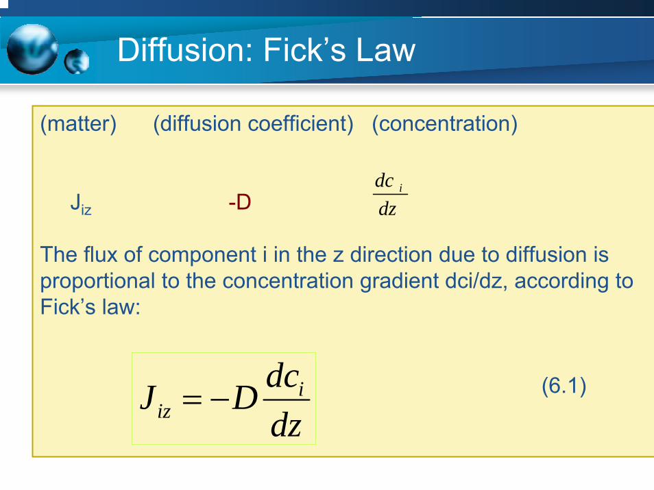
Diffusion: Fick’s Law
dtdn
AJ N
1=
(matter) (diffusion coefficient) (concentration)
Jiz -D
The flux of component i in the z direction due to diffusion is proportional to the concentration gradient dci/dz, according to Fick’s law:
(6.1)
dzdc i
dzdcDJ i
iz −=
Diffusion: Fick’s Law
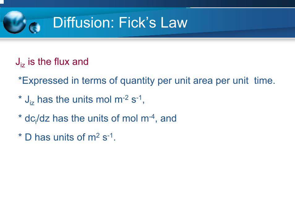
Jiz is the flux and
*Expressed in terms of quantity per unit area per unit time.
* Jiz has the units mol m-2 s-1,
* dci/dz has the units of mol m-4, and
* D has units of m2 s-1.

Diffusion: Fick’s Law
* The negative sign comes from the fact that if Ci increases in
the positive z direction dCi /dz is positive, but the flux is in the
negative z direction because the flow is in the direction of
lower concentrations

Determination of D for the diffusion of one gas into another
• The sliding partition is withdrawn for a
definite interval of time.
• From the average composition of one
chamber or the other, After a time
interval, D may be calculated.
Light gas
Slidingpartition
Heavy

Thermal Conduction: Fourier’s Law
Transport of heat is due to a gradient in temperature.
(heat) ( thermal conductivity) ( temperature)
qz
(6.2)
dzdTKq Tz −=∴
= - KT dzdT
K is the thermal conductivity.qz has the units of J m-2 s-1 anddT/dz has the units of K m-1, KT has the units of J m-1 s-1 K-1. The negative sign indicates that if dT/dz is positive, the flow
of heat is in the negative z direction, which is the direction toward lower temperature.

Thermal Conduction: Fourier’s Law
Viscosity: is a measure of the resistance that a fluid offers to
an applied shearing force.
• Consider what happens to the fluid between parallel
planes
• when the top plane is moved in the y direction at a
constant speed relative to the bottom plane while
maintaining a constant distance between the planes
(coordinate z)

Thermal Conduction: Fourier’s Law
• The planes are considered to be very large, so that edge
effects may be ignored.
• The layer of fluid immediately adjacent to the moving plane
moves with the velocity of this plane.
• The layer next to the stationary plane is stationary; in
between the velocity usually changes linearly with distance,.

Thermal Conduction: Fourier’s Law
The velocity gradient
Rate of change of velocity with respect to distance measured perpendicular to the direction of flow is represented by
duy/ dz
The viscosity η is defined by the equation
(6.3)dzdu
F yη−=
Thermal Conduction: Fourier’s Law
• F is the force per unit area required to move one plane
relative to the other.
• The negative sign comes from the fact that if F is in the +y
direction, the velocity uy decreases in successive layers away
from the moving plane and duy/dz is negative.

Thermal Conduction: Fourier’s Law
•The thermal conductivity is determined
by the hot wire method
• Determination of the rate of flow
through a tube, the torque on a disk that
is rotated in the fluid, or other
experimental arrangement.
• The outer cylinder is rotated at a
constant velocity by an electric motor.

Thermal Conduction: Fourier’s Law
• Since 1N = 1 kg m s-2, 1 Pa s = 1 kg m-1 s-1. A fluid has a
viscosity of 1 Pa s if a force of 1 N is required to move a
plane of 1 m2 at a velocity of 1 m s-1 with respect to a plane
surface a meter away and parallel with it.
• The cgs unit of viscosity is the poise, that is, 1 gs-1cm-1
0.1 Pa S = 1 poise.
Calculation of Transport Coefficients
To calculate the transport coefficients
D, KT, and η
even for hard-sphere molecules, needs to consider how
the Maxwell-Boltzmann distribution is disturbed by a
gradient of concentration, temperature or velocity.
Diffusion Coefficient
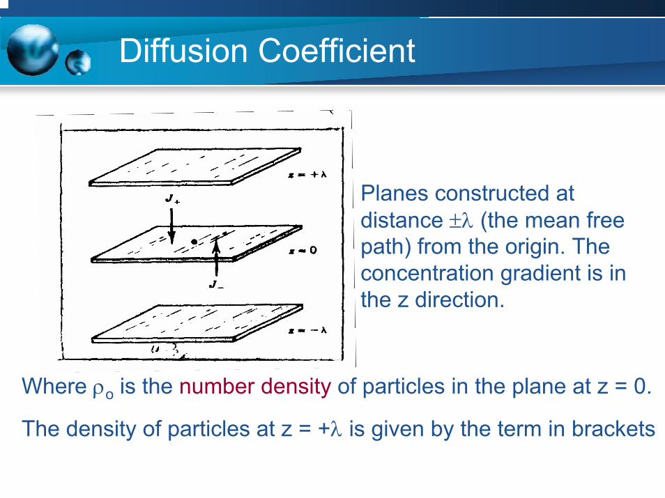
Planes constructed at distance ±λ (the mean free path) from the origin. The concentration gradient is in the z direction.
Where ρo is the number density of particles in the plane at z = 0.
The density of particles at z = +λ is given by the term in brackets
Diffusion Coefficient
• Consider the diffusion of molecules in a concentration gradient in the z direction and we are at z = 0.
• Imagine that we construct planes parallel to the xy plane at x = ±λ, where λ is the mean free path.
• We choose planes at the mean free path because molecules form more distant points will, on average, have suffered collisions before reaching z = 0.
Diffusion Coefficient
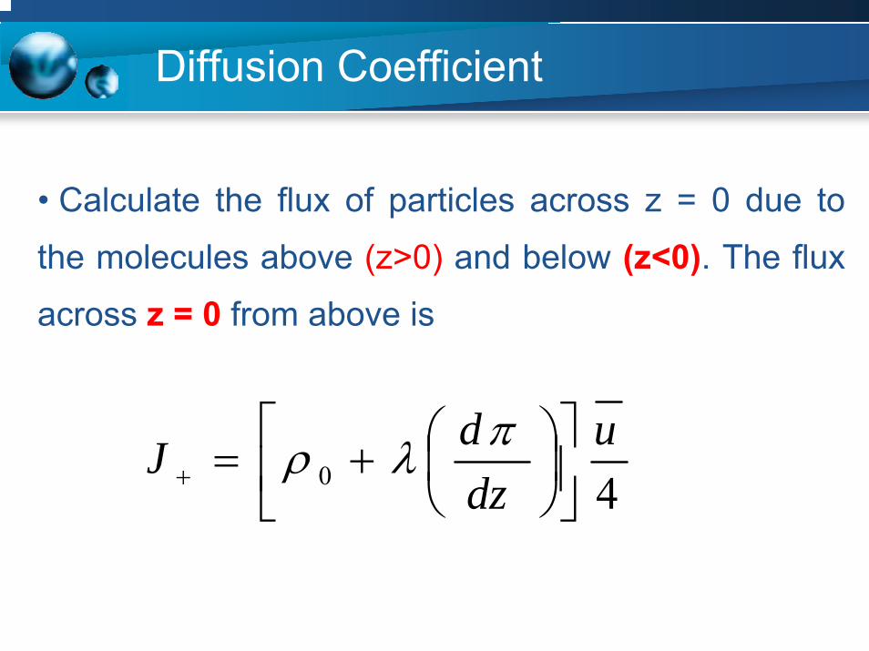
• Calculate the flux of particles across z = 0 due to
the molecules above (z>0) and below (z<0). The flux
across z = 0 from above is
40u
dzdJ ⎥
⎦
⎤⎢⎣
⎡⎟⎠⎞
⎜⎝⎛+=+
πλρ
Diffusion Coefficient
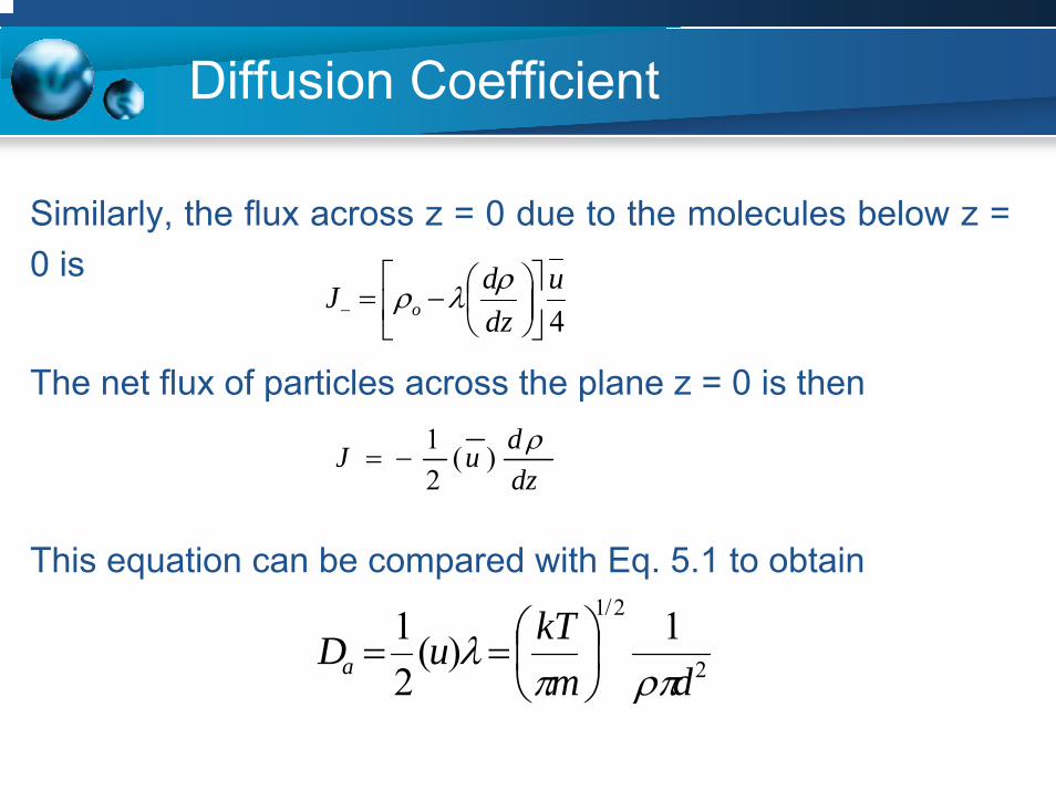
Similarly, the flux across z = 0 due to the molecules below z = 0 is
The net flux of particles across the plane z = 0 is then
This equation can be compared with Eq. 5.1 to obtain
4u
dzdJ o ⎥
⎦
⎤⎢⎣
⎡⎟⎠⎞
⎜⎝⎛−=−ρλρ
dzduJ ρ)(
21
−=
2
2/1 1)(21
dmkTuDa ρππ
λ ⎟⎠⎞
⎜⎝⎛==
Diffusion Coefficient
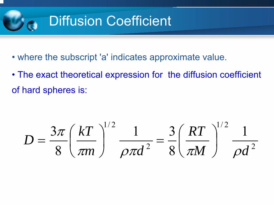
• where the subscript 'a' indicates approximate value.
• The exact theoretical expression for the diffusion coefficient
of hard spheres is:
2
2/1
2
2/1 1831
83
dMRT
dmkTD
ρπρπππ
⎟⎠⎞
⎜⎝⎛=⎟
⎠⎞
⎜⎝⎛=

Example 6.1
Predict D(O2,N2) of an equimolar mixture of O2 and N2 gases at 1.00 atm and 00C using dO2 = 0.353 nm and dN2 = 0.373 nm.____________________________________________________________________________________________________________________________________
RTPN
VnN
VN AA ===ρ 325
113
123
1069.2)273)(m 314.8(
10Pa)(6.022x 325.101( −−−
−
==∴ mxKmolPaK
molρ
= (0.353 nm + 0.373 nm)/2 = 0.363 nm),( 22 NOd2/1
1-3
11-
),( )mol kg 1000.32(K) 273)(JK 314.0(
83
22 ⎥⎦
⎤⎢⎣
⎡= −
−
xmold NO π
1251-3210 1059.1)mol 1064.2()1063.3(
1 −−−− = smx
kgxmxx
Example 6.1
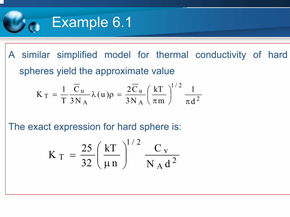
A similar simplified model for thermal conductivity of hard
spheres yield the approximate value
The exact expression for hard sphere is:
2
2/1
A
u
A
uT
d1
mkT
N3C2)u(
N3C
T1K
π⎟⎠⎞
⎜⎝⎛π
=ρλ=
2A
v2/1
TdN
Cn
kT3225K ⎟⎟
⎠
⎞⎜⎜⎝
⎛µ
=
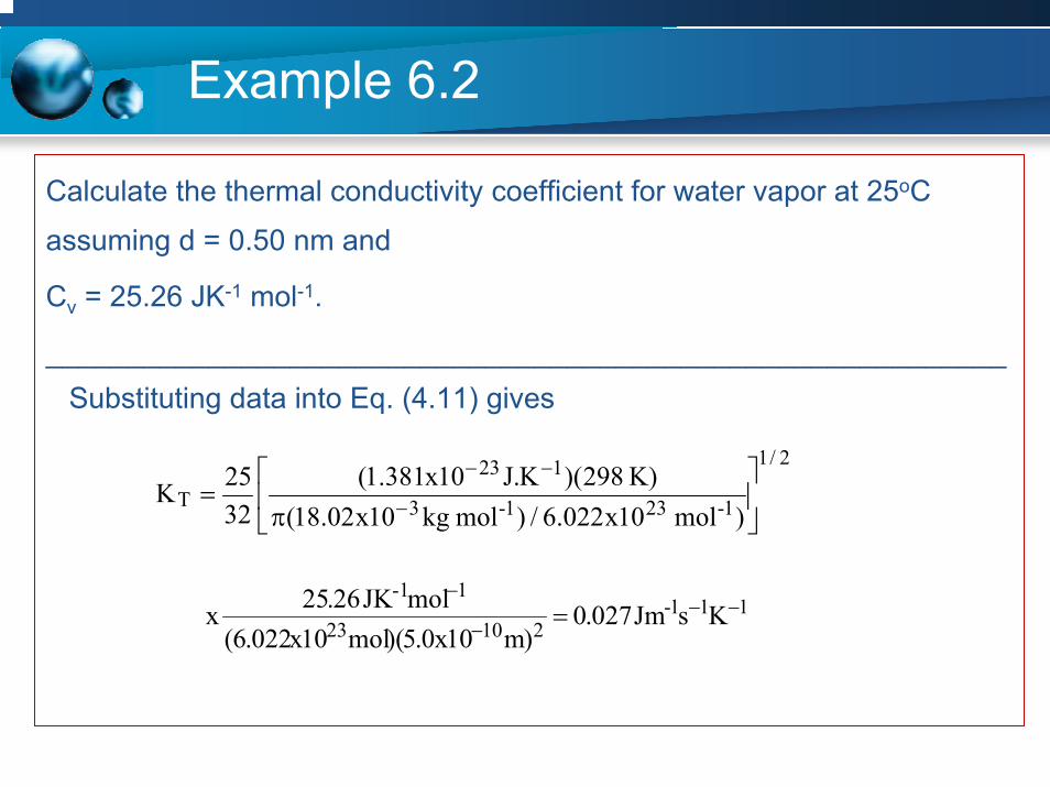
Example 6.2
Calculate the thermal conductivity coefficient for water vapor at 25oC
assuming d = 0.50 nm and
Cv = 25.26 JK-1 mol-1.
___________________________________________________________Substituting data into Eq. (4.11) gives
2/1
1-231-3
123T
)mol 10x022.6/)mol kg10x02.18(K) 298)(K.J10x381.1(
3225K ⎥
⎦
⎤⎢⎣
⎡
π= −
−−
111-21023
1-1KsJm 027.0
)m10x0.5)(mol10x022.6(molJK 26.25x −−
−
−=

Example 6.2
2
2/1
adm
mkT
32m)u(
31
π⎟⎠⎞
⎜⎝⎛π
=λρ=η
Finally, the approximate model for the viscosity of hard spheresyields:
whereas the exact expression for hard spheres is
2
2/1
dm
mkT
2323
⎟⎠⎞
⎜⎝⎛π
=η

Example 2
Note that this does not imply that real molecules are hard
spheres; in fact, we are forcing a model on the
experiment. Nevertheless, the results in Table 6.1 show
that a consistent set of molecular diameters result from
this analysis of the data.
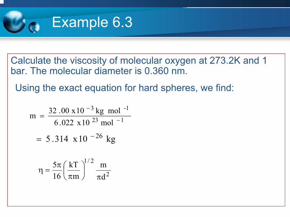
Example 6.3
Calculate the viscosity of molecular oxygen at 273.2K and 1 bar. The molecular diameter is 0.360 nm.
Using the exact equation for hard spheres, we find:
123
-13
mol10x022.6mol kg10x00.32m −
−=
kg10x314.5 26−=
2
2/1
dm
mkT
165
π⎟⎠⎞
⎜⎝⎛π
π=η
Example 3
29
262/1
26
123
)m10x360.0(kg10x314.5
)kg10x314.5()K2.273(JK10x380.1(
165
−
−
−
−−
π⎥⎦
⎤⎢⎣
⎡
ππ
=
= 1.926 x 10⁻⁵ kg m-1 s-1


![Chapter 22: Kinetic Theory of Warm Plasmas [version 1222.1.K]](https://static.fdokumen.com/doc/165x107/631d6102f7af5f2ec200e245/chapter-22-kinetic-theory-of-warm-plasmas-version-12221k.jpg)