J. Fluid Mech. (1999), vol. 389, pp. 391–411. Printed in the United Kingdom

c© 1999 Cambridge University Press

391

Kinetic theory of simple granular shear flows ofsmooth hard spheres

By J. M. M O N T A N E R O1, V. G A R Z O2,A. S A N T O S2 AND J. J. B R E Y3

1 Departamento de Electronica e Ingenierıa Electromecanica, Universidad de Extremadura,E-06071 Badajoz, Spain

2 Departamento de Fısica, Universidad de Extremadura, E-06071 Badajoz, Spain3 Fısica Teorica, Universidad de Sevilla, E-41080 Sevilla, Spain

(Received 4 June 1998 and in revised form 9 February 1999)

Steady simple shear flows of smooth inelastic spheres are studied by means of amodel kinetic equation and also of a direct Monte Carlo simulation method. Bothapproaches are based on the Enskog equation and provide for each other a test ofconsistency. The dependence of the granular temperature and of the shear and normalstresses on both the solid fraction and the coefficient of restitution is analysed. Quite agood agreement is found between theory and simulations in all cases. Also, simplifiedexpressions based on the analytical solution of the model for small dissipation areshown to describe fairly well the simulation results even for not small inelasticity. Acritical comparison with previous theories is carried out.

1. IntroductionIn rapid granular flows, particle interactions can be described as instantaneous

collisions and the motion of individual grains is analogous to the thermal motion ofmolecules in a gas. However, collisions between granular particles are inelastic andfrictional, so that the extension of the kinetic theory of molecular gases accounts forthese dissipation mechanisms (Jenkins & Savage 1983; Lun et al. 1984; Jenkins &Richman 1985; Goldshtein & Shapiro 1995; Brey, Dufty & Santos 1997a). In thesimplest versions, the grains are modelled as smooth, inelastic, hard spheres or disks.Inelasticity is characterized by means of a constant coefficient of normal restitution.In this way, generalizations of the Boltzmann and Enskog equations for inelasticparticles have been derived. From these kinetic equations, exact macroscopic balanceequations are easily obtained by taking appropriate velocity moments. Nevertheless,they only provide a true closed hydrodynamic description after explicit expressions forthe pressure tensor, the heat flux and energy source term are obtained. This requires,in general, solving the kinetic equation under consideration.

Almost all analytical studies of the Boltzmann and Enskog equations have beenrestricted to near equilibrium situations, for which approximate solutions to theequations have been found. Very little is known about solutions describing far fromequilibrium states. This is true for both molecular fluids and granular flows, but thedifficulties are even harder for the latter, since dissipation in collisions is coupled tospatial inhomogeneities in a rather non-trivial way. For instance, it is easily seen thata granular system with uniform boundaries at constant temperature develops spatialinhomogeneities spontaneously (Brey & Cubero 1998).

392 J. M. Montanero, V. Garzo, A. Santos and J. J. Brey

One of the simplest non-equilibrium states one can think of is simple or uniformshear flow. Macroscopically, it is characterized by a constant linear velocity profileand uniform density and temperature. This state has been extensively studied formolecular as well as for granular systems. Nevertheless, the nature of the state isquite different in each system. While for elastic fluids the temperature increasesmonotonically in time due to viscous heating, a steady state is possible for granularmedia when the effect of the viscosity is exactly compensated by the dissipation incollisions. It is precisely this steady state that we are interested in here.

Although steady simple shear flow has been the subject of many previous works,most of them are based on a Navier–Stokes description of the hydrodynamic fieldsand, therefore, they are restricted to small velocity gradients, which for this state isequivalent to small inelasticity. This was the method used by Lun et al. (1984) toget the rheological properties as functions of the coefficient of restitution and thedensity. On the other hand, the only general theory for arbitrary shear rate we areaware of was formulated by Jenkins & Richman (1988). They used a maximum-entropy approximation in the Enskog equation to get a closed set of equations for theelements of the pressure tensor. The equations are too complicated to be solved ingeneral, and additional approximations were introduced in order to analyse the limitsof dilute and dense systems. The theory predicts anisotropy of the pressure tensor,i.e. normal stress differences, an effect that cannot be derived from the Navier–Stokesapproximation. In this context, let us mention that Sela, Goldhirsch & Noskowicz(1996) have been able to obtain a perturbative solution of the Boltzmann equationup to Burnett order, i.e. transport equations to third order in the shear rate. At thisorder the normal stress differences show up.

The aim of this paper is to carry out a detailed study of the steady simple shear flowin the framework of the Enskog theory. Two complementary routes will be employed:a model kinetic equation and direct Monte Carlo simulations. Model kinetic equationsthat preserve the critical physical and mathematical properties of the original Enskogor Boltzmann equations are useful in order to allow a detailed analysis of granularflows. Here we will use a model for inelastic gases (Brey et al. 1997a) that hasbeen introduced very recently as an approximation of the Enskog equation or, moreprecisely, of a modified version of it, the so-called revised Enskog theory (RET) (vanBeijeren & Ernst 1973; Brey et al. 1997a). On the other hand, a very efficient numericalMonte Carlo simulation method has been proposed recently (Montanero & Santos1996, 1997a). It is an extension to the RET of the direct simulation Monte Carlomethod developed over the past twenty years for solving the Boltzmann equationfor molecular fluids (Bird 1994). The method is equally suitable for both elasticand inelastic collisions. Comparison between the model kinetic predictions and thesimulation results allows us to derive approximate expressions for the elements of thepressure tensor as explicit functions of the density and the coefficient of restitution.

The organization of the paper is as follows. In §2 the model kinetic equationis introduced and its derivation from the RET is briefly discussed. The model isparticularized for steady simple shear flow in §3, where a method to obtain numericallythe elements of the pressure tensor in the first Sonine approximation is discussed indetail. In the limit of small dissipation it is possible to derive explicit analyticalexpressions for these elements. Section 4 deals with the Monte Carlo simulation ofthe RET equation particularized for steady simple shear flow. The results are presentedand discussed in §5, where a simplified expression for the pressure tensor is introducedand seen to agree well with the simulations. The one-particle distribution functionis also considered. The rheological properties are compared with those derived from

Simply sheared granular flow 393

the well-known theory developed by Lun et al. (1984), while a comparison with themaximum-entropy approximation for the distribution function is also carried out.Finally, §6 provides a short summary and conclusions.

2. Description of the modelThe model kinetic equation we will use in the following was introduced as an

approximate representation of the revised Enskog theory (RET) for a dense gas ofsmooth inelastic hard spheres of mass m and diameter σ. Inelasticity in collisions isintroduced through a constant coefficient of normal restitution α. The RET gives anevolution equation for the single-particle distribution function, f(r, v, t) (Brey et al.1997a) (

∂

∂t+ v1 · ∇1

)f(r1, v1, t) = JE[r1, v1|f(t)], (2.1)

where JE is the Enskog collision operator

JE[r1, v1|f(t)] = σ2

∫dv2

∫dσΘ(g · σ)(g · σ)

[α−2f(2)(r1, r1 − σ, v′1, v′2, t)−f(2)(r1, r1 + σ, v1, v2, t)

]. (2.2)

Here,

f(2)(r1, r2, v1, v2, t) = χ[r1, r2|n(t)]f(r1, v1, t)f(r2, v2, t), (2.3)

with χ[r1, r2|n(t)] being the equilibrium pair correlation function as a functional ofthe non-equilibrium density field

n(r, t) =

∫dv f(r, v, t). (2.4)

Moreover, Θ is the Heaviside step function, σ is a unit vector, σ = σσ, g = v1 − v2

and

v′1 = v1 − 1 + α

2α(g · σ)σ, (2.5a)

v′2 = v2 +1 + α

2α(g · σ)σ (2.5b)

are the precollisional velocities yielding (v1, v2) as postcollisional ones. Balance equa-tions for number of particles, momentum and energy are derived from (2.1) bymultiplying by 1, mv1 and mv2

1/2, respectively, and integrating over v1. Defining theflow velocity u(r, t) and the local (granular) temperature T (r, t) in the standard way,

n(r, t)u(r, t) =

∫dv vf(r, v, t), (2.6)

32n(r, t)T (r, t) =

∫dv 1

2mV 2(r, t)f(r, v, t), (2.7)

where V (r, t) = v − u(r, t), results in

∂n

∂t+ ∇ · (nu) = 0, (2.8)

394 J. M. Montanero, V. Garzo, A. Santos and J. J. Brey

∂u

∂t+ u · ∇u+ (mn)−1∇ · P = 0, (2.9)

∂T

∂t+ u · ∇T +

2

3n

[P :∇u+ ∇ · q + (1− α2)ω

]= 0. (2.10)

The expressions for the pressure tensor, P , and the heat flux, q, contain both ‘kinetic’and ‘collisional transfer’ contributions,

P = Pk + Pc, q = qk + qc. (2.11)

They are given by

Pk(r, t) =

∫dvmVV f(r, v, t), (2.12)

qk(r, t) =

∫dvm

2V 2V f(r, v, t), (2.13)

Pc(r, t) =1 + α

4mσ3

∫dv1

∫dv2

∫dσΘ(g · σ)(g · σ)2σσF(r, σ, v1, v2, t), (2.14)

qc(r, t) =1 + α

4mσ3

∫dv1

∫dv2

∫dσΘ(g · σ)(g · σ)2(G · σ)σF(r, σ, v1, v2, t). (2.15)

In the above expressions, G = 12(v1 + v2)− u and we have introduced

F(r, σ, v1, v2, t) =

∫ 1

0

dλ f(2)(r − (1− λ)σ, r + λσ, v1, v2, t). (2.16)

A derivation of (2.14)–(2.16) for the elastic limit α = 1 is given in Appendix Bof Santos et al. (1998). The generalization to arbitrary coefficient of restitution isstraightforward. Finally, the term (1 − α2)ω in (2.10) describes the rate of energydissipation in collisions due to inelasticity. The explicit expression for ω is

ω(r, t) =m

8σ2

∫dv1

∫dv2

∫dσΘ(g · σ)(g · σ)3f(2)(r, r + σ, v1, v2, t). (2.17)

The complexity of the RET has limited its use to states near equilibrium. Even in theelastic limit α = 1, almost nothing is known about solutions corresponding to far fromequilibrium situations. This has lead to the introduction of model kinetic equations,in which the collision operator is replaced by a simpler form that, nevertheless, retainsthe relevant physical and mathematical properties of the original one. Here we willuse a model that has been proposed very recently (Dufty, Brey & Santos 1997).The model has already been applied to the study of both dissipative systems in thelow-density, or Boltzmann, limit (Brey, Ruiz-Montero & Moreno 1997b) and densesystems in the elastic limit (Santos et al. 1998). In this paper a dense dissipativesystem will be considered.

The starting point for the formulation of the model kinetic equation is to representthe collision operator JE as an expansion in a complete set of velocity polynomials,with a scalar product weighted with the local equilibrium distribution. The functionalform of the contribution in the subspace spanned by 1, v, and v2 is retained exactly. Onthe other hand, the contribution from the subspace orthogonal to that is approximatedby a single relaxation term plus a correction that takes into account that the Enskogcollision operator does not vanish for the local equilibrium distribution function. Thedetails of the reasoning and calculations leading to the model equation have been

Simply sheared granular flow 395

presented elsewhere (Dufty et al. 1997b; Santos et al. 1998). Therefore, we only reporthere the resulting equation:(

∂

∂t+ v · ∇

)f = −ζ (f − f`) +

1

Tf` [A :D(V ) + B · S(V )]− 1

nTf`

{V∇ : Pc

+( m

3TV 2 − 1

) [∇ · qc + Pc :∇u+ (1− α2)ω]}

, (2.18)

where

f`(r, v, t) = n( m

2πT

)1/2

exp(−mV 2/2T

)(2.19)

is the local equilibrium distribution function and

D(V ) = m(VV − 1

3V 2I), S(V ) =

(12mV 2 − 5

2T)V , (2.20)

A =1

2nT

∫dV D(V )JE[f`], B =

2m

5nT 2

∫dV S(V )JE[f`]. (2.21)

In (2.20) I denotes the unit tensor. The model equation (2.18) contains the effectivecollision frequency ζ. In practical applications it can be fixed by requiring that themodel reproduces some quantitative property of the (exact) Enskog equation, forinstance the value of a given transport coefficient. Let us stress that the model notonly reproduces by construction the form of the exact balance equations (2.8)–(2.10)following from the RET, but the expressions for the fluxes and the energy sourceterms are given by the same functionals of the distribution function as in the RET,cf. (2.14)–(2.17).

3. Solution of the model for simple shear flowAs stated in the Introduction, simple shear flow is characterized by a linear profile

of the flow velocity: u(r) = a · r, where the elements of the tensor a are aij = aδixδjy ,a being the constant shear rate. Otherwise, the number density n and the granulartemperature T are uniform. The temperature changes in time due to the competitionbetween two mechanisms: on the one hand, viscous heating and, on the other hand,energy dissipation in collisions. In the steady state, both mechanisms cancel eachother and the temperature remains constant. In that case, according to the energybalance equation (2.10), the shear stress Pxy and the sink term ω are related by

aPxy = −(1− α2)ω. (3.1)

This steady simple shear flow is the problem we want to analyse by means of thekinetic model described in §2, as well as by performing Monte Carlo simulations ofthe Enskog equation.

All the spatial dependence of the velocity distribution function occurs through thepeculiar velocity V = v− u(r): f(r, v)→ f(V ). Consequently, the kinetic model (2.18)becomes(

ζ − aVy ∂

∂Vx

)f(V ) = ζf`(V )

[1 +

1

nTζ

( m3T

V 2 − 1)Pkxya+

1

TζA :D(V )

]≡ ζf`(V ), (3.2)

where we have taken into account (3.1), that the pressure tensor is uniform and

396 J. M. Montanero, V. Garzo, A. Santos and J. J. Brey

that, by symmetry reasons, the heat flux q and the vector B vanish. For the collisionfrequency we will take the following:

ζ = 165π1/2nσ2χ(T/m)1/2 , (3.3)

so that the Enskog shear viscosity coefficient for elastic spheres is recovered (Duftyet al. 1997). The solution to (3.2) can be formally written as

f(V ) =

∫ ∞0

ds e−sf`(V +

s

ζa · V

). (3.4)

This solution is not complete, since we need to know the quantities T , Pkxy , and Aij

for given values of a, n, and α. The tensor Aij is determined entirely by the localequilibrium distribution f`, cf. (2.21), so that it only depends on T . Its non-zeroelements are

Axy = −4π

15(T/m)1/2nσ2χa

1 + α

2

[12(3α− 1) + 1

7(1 + α)a2

], (3.5)

Axx = Ayy = − 12Azz

= (T/m)1/2nσ2χ

∫dσ(σ2

x − 13)aσxσy

1 + α

2

{(1 + α)

π1/2aσxσye

−a2σ2xσ

2y

+erf (aσxσy)[

12(3α− 1) + (1 + α)a2σ2

xσ2y

]− 1

π1/2(1− α)e−a2σ2

xσ2y

aσxσy

}, (3.6)

where erf denotes the error function, a ≡ 12aσ(m/T )1/2 and we have taken into account

that χ(n) is a constant in our problem. The relationship between Pkxy and T is easily

found by multiplying both sides of (3.4) by mVxVy and integrating over velocity space.The result is

Pkxy = −nT a

ζ

(1 +

2a

3nTζP kxy − 2

Axy

a+ 2

Axx

ζ

). (3.7)

In order to close the problem, we need an extra condition. This is provided by (3.1),where P c

xy and ω are determined by replacing f by the right-hand side of (3.4) in theequations

P cij =

1 + α

4mσ3χ

∫dσσiσj

∫dV 1

∫dV 2Θ(σ · g)(σ · g)2f(V 1 + a · σ)f(V 2), (3.8)

ω =mσ2

8χ

∫dσ

∫dV 1

∫dV 2Θ(σ · g)(σ · g)3f(V 1 + a · σ)f(V 2), (3.9)

which follow from (2.14) and (2.17), respectively. Once Pkxy and T are known, the

remaining elements of the pressure tensor can be obtained. Their kinetic parts are

P kxx = nT

(1− 4a

3nTζP kxy + 2

Axx

ζ

), (3.10)

P kyy = nT

(1 +

2a

3nTζP kxy + 2

Axx

ζ

), (3.11)

P kzz = nT

(1 +

2a

3nTζP kxy − 4

Axx

ζ

). (3.12)

The corresponding collisional parts are evaluated using (3.8).

Simply sheared granular flow 397

Although the problem of solving the kinetic model for steady simple shear flow isclosed, the numerical integrations in (3.8) and (3.9) are very intricate. Thus, from apractical point of view, it is more convenient to take the first Sonine approximation(Chapman & Cowling 1970) for f in those equations, rather than the solution (3.4).This strategy proved to be useful in the elastic case (Santos et al. 1998) and, aswill be seen in §5, the agreement with Monte Carlo simulations is also good in theinelastic case. In the first Sonine approximation, f(V ) → f`(V ) [1 + C : D(V )/ 2T ],where

C =1

nTPk − I . (3.13)

With this approximation, the evaluation of P cij and ω is similar to that of the tensor

Aij . The result is

P cij = −1 + α

4nTn∗χ

∫dσ σiσj

{2

π1/2aσxσye

−a2σ2xσ

2y − (1 + 2a2σ2

xσ2y

)erfc (aσxσy)

− (σσ − 13I)

: C erfc (aσxσy)− 18

[(σσ − 1

3I)

: C]2 2

π1/2aσxσye

−a2σ2xσ

2y

}, (3.14)

ω = nTnσ2χ(T/m)1/2

∫dσ

{1

2π1/2

(1 + a2σ2

xσ2y

)e−a

2σ2xσ

2y

+ 14

(3 + 2a2σ2

xσ2y

)aσxσyerf (aσxσy)

+ 32

(σσ − 1

3I)

: C

[1

2π1/2e−a

2σ2xσ

2y + 1

2aσxσyerf(aσxσy)

]+ 3

32

[(σσ − 1

3I)

: C]2 1

π1/2e−a

2σ2xσ

2y

}. (3.15)

Here, n∗ ≡ nσ3 is the reduced number density. It is related to the solid fraction ν byν = 1

6πn∗. In summary, (3.7) and (3.10)–(3.12) allow one to express C as a function

of T ; when (3.14) and (3.15) are used in (3.1), one gets a closed equation for thetemperature T , that can be solved numerically.

It is interesting to consider the limit of low dissipation, in which case it is possibleto get analytical results and the Sonine approximation is not needed. To that end, weintroduce the perturbation parameter ε ≡ 1−α2 and perform a power series expansionaround ε = 0. The details of the calculation are presented in the Appendix and herewe only give the final results. First, the expression for the granular temperature isgiven through the ratio a/ζ (which measures the shear rate in units of the collisionfrequency) as

a

ζ= a1(1− α2)1/2 + a3(1− α2)3/2 + · · · . (3.16)

Next, the elements of the pressure tensor can be written as

1

nTPxx = 1 +

2π

3n∗χ+

(Pkxx,2 + P c

xx,2

)a2

1(1− α2) + · · · , (3.17)

1

nTPyy = 1 +

2π

3n∗χ+

(Pkyy,2 + P c

yy,2

)a2

1(1− α2) + · · · , (3.18)

398 J. M. Montanero, V. Garzo, A. Santos and J. J. Brey

1

nTPzz = 1 +

2π

3n∗χ+

(Pkzz,2 + P c

zz,2

)a2

1(1− α2) + · · · , (3.19)

ζ

a

1

nTPxy = Pk

xy,1 + P cxy,1 +

(Pkxy,3 + P c

xy,3

)a2

1(1− α2) + · · · . (3.20)

In these equations, a1, a3, Pkij,`, and P c

ij,` are dimensionless coefficients that depend onthe density and are explicitly given in the Appendix.

In what follows, we will use the Carnahan & Starling (1969) approximation for thedensity dependence of the pair correlation function at contact:

χ(ν) =1− 1

2ν

(1− ν)3. (3.21)

Of course, one could take any other approximation for χ since the simulation andtheory results depend on density only through the product νχ(ν).

4. Monte Carlo simulationRecently, Montanero & Santos (1996, 1997a) have proposed a simulation Monte

Carlo (ESMC) algorithm that solves the Enskog equation for a system of elastichard spheres, in the same spirit as the well-known DSMC method for solving theBoltzmann equation (Bird 1994). The extension of the ESMC method to deal withinelastic collisions is straightforward (Brey et al. 1997a). In the particular case ofsimple shear flow, the simulation method is especially easy to implement, due tothe fact that this state is homogeneous in the local Lagrangian frame. This is animportant advantage with respect to molecular dynamics simulations. In contrast, therestriction to this quasi-homogeneous state prevents us from analysing the possibleinstability of simple shear flow or the formation of microstructures.

The ESMC method, as applied to simple shear flow, proceeds as follows (Montanero& Santos 1997b). The one-particle distribution function is represented by the peculiarvelocities {V r} of a sample of N ‘simulated’ particles:

f(V , t)→ n1

N

N∑r=1

δ(V − V r(t)). (4.1)

The velocities are updated at integer times t = ∆t, 2∆t, 3∆t, . . ., where the time step ∆tis much smaller than the mean free time and the inverse shear rate. This is done intwo stages: free streaming and collisions. In the local Lagrangian frame, the particlesare subjected to the action of a non-conservative inertial force F = −ma · V . This isrepresented by the second term on the left-hand side of (3.2). Thus, the free-streamingstage consists of making V r → V r − a · V r∆t. In the collision stage, a sample of12Nwmax pairs is chosen at random with equiprobability, where wmax is an upper

bound estimate of the probability that a particle collides in the time interval betweent and t+ ∆t. For each pair rs belonging to this sample, the following steps are taken:(1) a given direction σrs is chosen at random with equiprobability; (2) the collisionbetween particles r and s is accepted with a probability equal to Θ(σrs · grs)wrs/wmax,where wrs = 4πσ2χnσrs ·grs∆t and grs = V r−V s−σa·σrs; (3) if the collision is accepted,postcollisional velocities are assigned to both particles: V r → V r− 1

2(1+α)(σrs ·grs)σrs,

V s → V s + 12(1 + α)(σrs · grs)σrs. In the case that in one of the collisions wrs > wmax,

the estimate of wmax is updated as wmax = wrs. Typically, the fraction of particles thatchange their velocities due to collisions is of the order of wmax. This particularization

Simply sheared granular flow 399

0.6

0.4

0.2

0 10 20 30 40 50 60 70 80

t/t0

h

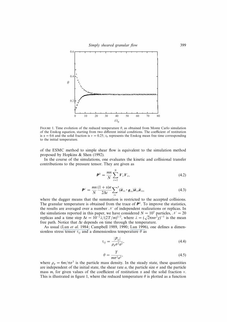
Figure 1. Time evolution of the reduced temperature θ, as obtained from Monte Carlo simulationof the Enskog equation, starting from two different initial conditions. The coefficient of restitutionis α = 0.6 and the solid fraction is ν = 0.25; t0 represents the Enskog mean free time correspondingto the initial temperature.

of the ESMC method to simple shear flow is equivalent to the simulation methodproposed by Hopkins & Shen (1992).

In the course of the simulations, one evaluates the kinetic and collisional transfercontributions to the pressure tensor. They are given as

Pk =mn

N

N∑r=1

V rV r, (4.2)

Pc =mn

N

(1 + α)σ

2∆t

∑rs

†(σrs · grs)σrsσrs, (4.3)

where the dagger means that the summation is restricted to the accepted collisions.The granular temperature is obtained from the trace of Pk . To improve the statistics,the results are averaged over a number N of independent realizations or replicas. Inthe simulations reported in this paper, we have considered N = 105 particles,N = 20replicas and a time step ∆t = 10−2λ/(2T/m)1/2, where λ = (

√2πnσ2χ)−1 is the mean

free path. Notice that ∆t depends on time through the temperature.As usual (Lun et al. 1984; Campbell 1989, 1990; Lun 1996), one defines a dimen-

sionless stress tensor τij and a dimensionless temperature θ as

τij =|Pij |ρpσ2a2

, (4.4)

θ =T

mσ2a2, (4.5)

where ρp = 6m/πσ3 is the particle mass density. In the steady state, these quantitiesare independent of the initial state, the shear rate a, the particle size σ and the particlemass m, for given values of the coefficient of restitution α and the solid fraction ν.This is illustrated in figure 1, where the reduced temperature θ is plotted as a function

400 J. M. Montanero, V. Garzo, A. Santos and J. J. Brey

4

3

2

02 4 6 8 10 12

(1–α2)–1

h

1

Figure 2. Plot of the reduced temperature θ versus the parameter (1 − α2)−1 for ν = 0.25, asobtained from simulation (circles), the numerical solution of the kinetic model (solid line), thesimplified solution of the model (dashed line) and the LSJC theory (dotted line).

of time for α = 0.6 and ν = 0.25, starting from two different initial conditions. It isevident that after a transient stage, a common steady state is reached. The durationof the transient stage is typically 30 collisions per particle.

5. ResultsIn this Section we will explore the dependence of τij and θ on the coefficient of

restitution α and the solid fraction ν. We will compare the results obtained fromMonte Carlo simulations with those from the kinetic model discussed in §2 and §3and with the well-known theory of Lun et al. (1984) (LSJC). In the latter theory, anapproach close to the Chapman–Enskog method is used, so that it is more justifiedin the ‘nearly elastic’ case.

First, we shall investigate the dependence of the relevant quantities on α for a givendensity. Recently, Goldhirsch & Tan (1996) have performed molecular dynamicssimulations of a dilute system of smooth inelastic disks and have found that thereduced temperature θ can be closely fitted by a linear function of (1 − α2)−1. Thesame result has been obtained from the solution of the kinetic model in the low-density limit by Brey et al. (1997b). Here we have observed the same behaviour fora finite density, both from the simulations and from the kinetic theory analyses. Asan illustrative example, we consider ν = 0.25. At this density, in the elastic case,the collisional contribution to the pressure is about twice the kinetic contribution.Figure 2 shows θ versus (1−α2)−1 as obtained from the simulations (circles), from thenumerical solution of the model (solid line), as described in §3, and from the LSJCtheory (dotted line). It is clear that the model has an excellent agreement with thesimulation results and also that θ is practically linear in (1− α2)−1. Thus, a very goodapproximation is

θ(ν, α) =θ1(ν)

1− α2+ θ2(ν). (5.1)

Simply sheared granular flow 401

0.9

0 0.2 0.4 0.6 0.71–α2

sii /h0.8

0.7

0.60.50.30.1

(c)

(b)

(a)

Figure 3. Plot of (a) τxx/θ, (b) τyy/θ and (c) τzz/θ versus 1−α2 for ν = 0.25. Symbols and lines havethe same meaning as in figure 2. Notice that in the LSJC theory the normal stresses are isotropic.

Consequently, the coefficients θ1,2(ν) in the model can be exactly obtained by com-paring the low-dissipation behaviour of (5.1) with (3.16). The results are

θ1 =25π

9216ν2χ2a21

, (5.2)

θ2 = − 25πa3

4608ν2χ2a31

. (5.3)

The function given by (5.1)–(5.3) is also plotted in figure 2 (dashed line). The factthat the dashed and the solid lines do not coincide exactly is due to the Sonineapproximation used to evaluate P c

ij and ω in the numerical solution of the model.While this approximation is consistent with the exact a1, it gives a small deviationfrom the exact a3. The LSJC theory overestimates the temperature, but it is alsoconsistent with a linear behaviour of the form (5.1). While the slope is exactly givenby (5.2), the line is shifted with respect to the simulation results. This is because theLSJC theory is based on a first-order (Navier–Stokes) Chapman–Enskog expansion,while the correct determination of θ2 requires going to third-order (super-Burnett).

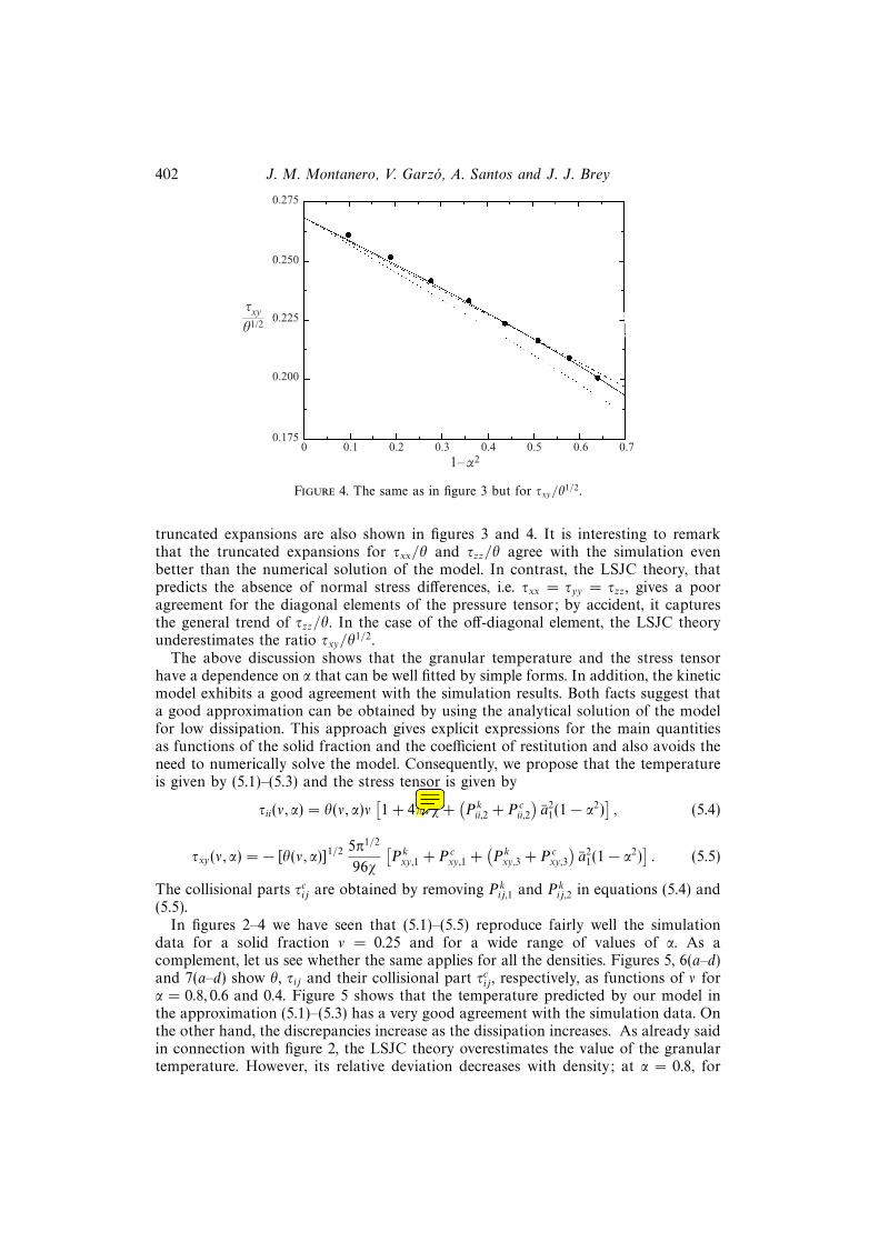
Apart from the temperature, the non-zero elements of the stress tensor, namelyτxx, τyy , τzz and τxy = τyx are the most relevant quantities. We have observed thatthe dependence of these elements on the coefficient of restitution is not well fittedby relations similar to that of (5.1). On the other hand, the solution of the modelin the low-density regime (Brey et al. 1997b) predicts that the ratios τii/θ, i =x, y, z, and τxy/θ

1/2 are linear functions of 1 − α2. Notice that τii/θ = νPii/nT andτxy/θ

1/2 = −(5π1/2/96χ)(ζ/nTa)Pxy . A natural question is whether the above simplebehaviours can be extended to dense systems. In figures 3 and 4 we plot τii/θand τxy/θ

1/2, respectively, as functions of 1 − α2 for ν = 0.25. The agreementof the model predictions with the simulation data is generally good, although thediscrepancies are larger than in the case of the temperature. We observe that theplotted quantities are indeed quasi-linear functions, especially in the case of thesimulation results. Consequently, one can obtain a good approximation by consideringthe low-dissipation expansions (3.17)–(3.20) truncated to the order 1 − α2. These

402 J. M. Montanero, V. Garzo, A. Santos and J. J. Brey

0.275

0 0.2 0.4 0.6 0.71–α2

sxy

h1/2

0.250

0.225

0.1750.50.30.1

0.200

Figure 4. The same as in figure 3 but for τxy/θ1/2.

truncated expansions are also shown in figures 3 and 4. It is interesting to remarkthat the truncated expansions for τxx/θ and τzz/θ agree with the simulation evenbetter than the numerical solution of the model. In contrast, the LSJC theory, thatpredicts the absence of normal stress differences, i.e. τxx = τyy = τzz , gives a pooragreement for the diagonal elements of the pressure tensor; by accident, it capturesthe general trend of τzz/θ. In the case of the off-diagonal element, the LSJC theoryunderestimates the ratio τxy/θ

1/2.The above discussion shows that the granular temperature and the stress tensor

have a dependence on α that can be well fitted by simple forms. In addition, the kineticmodel exhibits a good agreement with the simulation results. Both facts suggest thata good approximation can be obtained by using the analytical solution of the modelfor low dissipation. This approach gives explicit expressions for the main quantitiesas functions of the solid fraction and the coefficient of restitution and also avoids theneed to numerically solve the model. Consequently, we propose that the temperatureis given by (5.1)–(5.3) and the stress tensor is given by

τii(ν, α) = θ(ν, α)ν[1 + 4πνχ+

(Pkii,2 + P c

ii,2

)a2

1(1− α2)], (5.4)

τxy(ν, α) = − [θ(ν, α)]1/2 5π1/2

96χ

[Pkxy,1 + P c

xy,1 +(Pkxy,3 + P c

xy,3

)a2

1(1− α2)]. (5.5)

The collisional parts τcij are obtained by removing Pkij,1 and Pk

ij,2 in equations (5.4) and(5.5).

In figures 2–4 we have seen that (5.1)–(5.5) reproduce fairly well the simulationdata for a solid fraction ν = 0.25 and for a wide range of values of α. As acomplement, let us see whether the same applies for all the densities. Figures 5, 6(a–d)and 7(a–d) show θ, τij and their collisional part τcij , respectively, as functions of ν forα = 0.8, 0.6 and 0.4. Figure 5 shows that the temperature predicted by our model inthe approximation (5.1)–(5.3) has a very good agreement with the simulation data. Onthe other hand, the discrepancies increase as the dissipation increases. As already saidin connection with figure 2, the LSJC theory overestimates the value of the granulartemperature. However, its relative deviation decreases with density; at α = 0.8, for

Simply sheared granular flow 403

0.2 0.4 0.6 0.7ν

h

1

0.50.30.1

0.1

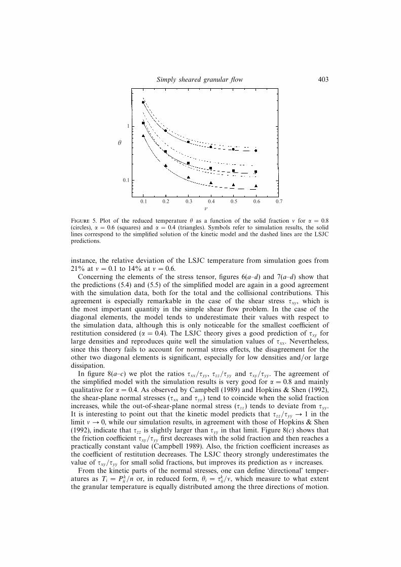
Figure 5. Plot of the reduced temperature θ as a function of the solid fraction ν for α = 0.8(circles), α = 0.6 (squares) and α = 0.4 (triangles). Symbols refer to simulation results, the solidlines correspond to the simplified solution of the kinetic model and the dashed lines are the LSJCpredictions.

instance, the relative deviation of the LSJC temperature from simulation goes from21% at ν = 0.1 to 14% at ν = 0.6.

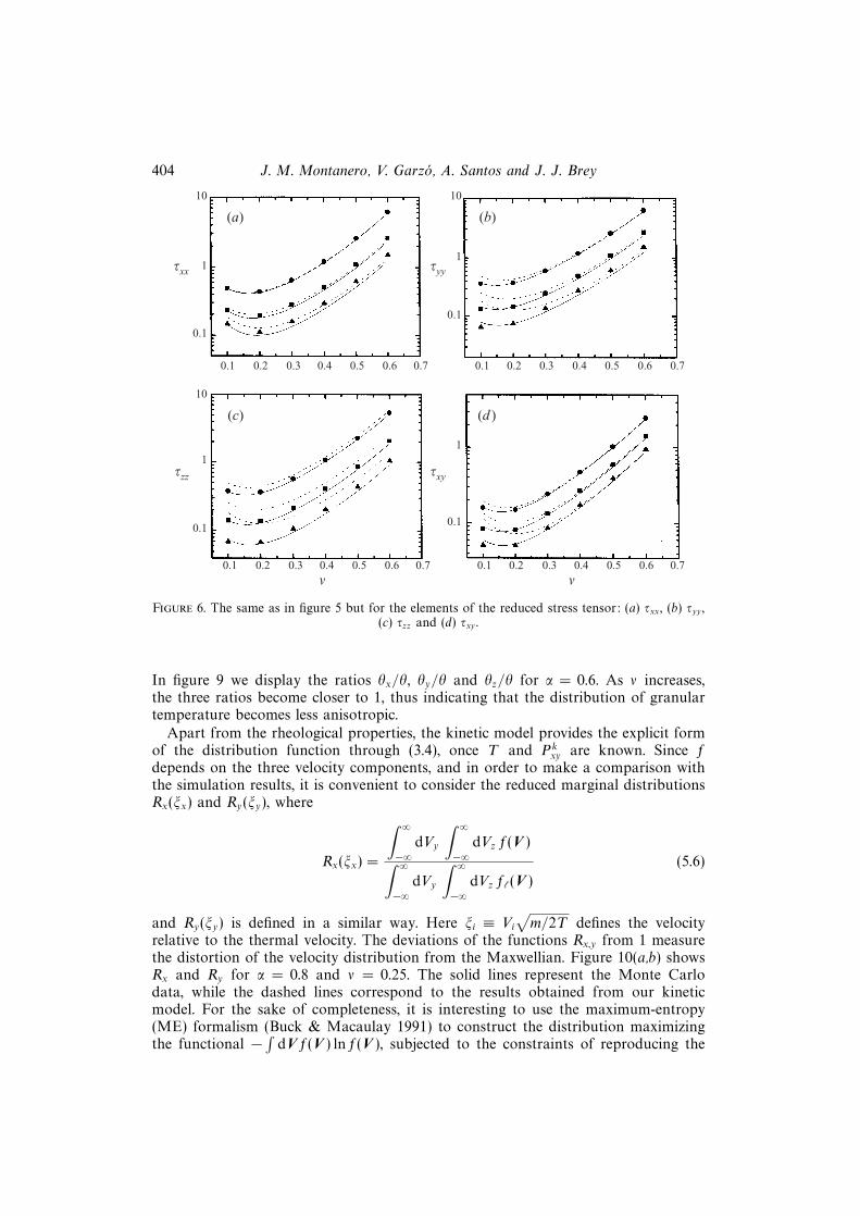
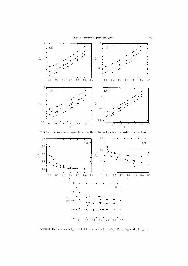
Concerning the elements of the stress tensor, figures 6(a–d) and 7(a–d) show thatthe predictions (5.4) and (5.5) of the simplified model are again in a good agreementwith the simulation data, both for the total and the collisional contributions. Thisagreement is especially remarkable in the case of the shear stress τxy , which isthe most important quantity in the simple shear flow problem. In the case of thediagonal elements, the model tends to underestimate their values with respect tothe simulation data, although this is only noticeable for the smallest coefficient ofrestitution considered (α = 0.4). The LSJC theory gives a good prediction of τxy forlarge densities and reproduces quite well the simulation values of τxx. Nevertheless,since this theory fails to account for normal stress effects, the disagreement for theother two diagonal elements is significant, especially for low densities and/or largedissipation.

In figure 8(a–c) we plot the ratios τxx/τyy , τzz/τyy and τxy/τyy . The agreement ofthe simplified model with the simulation results is very good for α = 0.8 and mainlyqualitative for α = 0.4. As observed by Campbell (1989) and Hopkins & Shen (1992),the shear-plane normal stresses (τxx and τyy) tend to coincide when the solid fractionincreases, while the out-of-shear-plane normal stress (τzz) tends to deviate from τyy .It is interesting to point out that the kinetic model predicts that τzz/τyy → 1 in thelimit ν → 0, while our simulation results, in agreement with those of Hopkins & Shen(1992), indicate that τzz is slightly larger than τyy in that limit. Figure 8(c) shows thatthe friction coefficient τxy/τyy first decreases with the solid fraction and then reaches apractically constant value (Campbell 1989). Also, the friction coefficient increases asthe coefficient of restitution decreases. The LSJC theory strongly underestimates thevalue of τxy/τyy for small solid fractions, but improves its prediction as ν increases.

From the kinetic parts of the normal stresses, one can define ‘directional’ temper-atures as Ti = Pk

ii /n or, in reduced form, θi = τkii/ν, which measure to what extentthe granular temperature is equally distributed among the three directions of motion.

404 J. M. Montanero, V. Garzo, A. Santos and J. J. Brey

10

1

0.1

0.1 0.2 0.3 0.4 0.5 0.6 0.7

10

1

0.1

0.1 0.2 0.3 0.4 0.5 0.6 0.7

10

1

0.1

0.1 0.2 0.3 0.4 0.5 0.6 0.7

1

0.1

0.1 0.2 0.3 0.4 0.5 0.6 0.7

(c)

(a)

(d )

(b)

m m

szz

sxx syy

sxy

Figure 6. The same as in figure 5 but for the elements of the reduced stress tensor: (a) τxx, (b) τyy ,(c) τzz and (d) τxy .

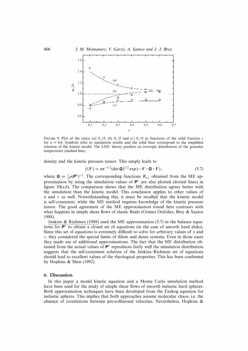
In figure 9 we display the ratios θx/θ, θy/θ and θz/θ for α = 0.6. As ν increases,the three ratios become closer to 1, thus indicating that the distribution of granulartemperature becomes less anisotropic.

Apart from the rheological properties, the kinetic model provides the explicit formof the distribution function through (3.4), once T and Pk

xy are known. Since fdepends on the three velocity components, and in order to make a comparison withthe simulation results, it is convenient to consider the reduced marginal distributionsRx(ξx) and Ry(ξy), where

Rx(ξx) =

∫ ∞−∞

dVy

∫ ∞−∞

dVz f(V )∫ ∞−∞

dVy

∫ ∞−∞

dVz f`(V )

(5.6)

and Ry(ξy) is defined in a similar way. Here ξi ≡ Vi√m/2T defines the velocity

relative to the thermal velocity. The deviations of the functions Rx,y from 1 measurethe distortion of the velocity distribution from the Maxwellian. Figure 10(a,b) showsRx and Ry for α = 0.8 and ν = 0.25. The solid lines represent the Monte Carlodata, while the dashed lines correspond to the results obtained from our kineticmodel. For the sake of completeness, it is interesting to use the maximum-entropy(ME) formalism (Buck & Macaulay 1991) to construct the distribution maximizingthe functional − ∫ dV f(V ) ln f(V ), subjected to the constraints of reproducing the

Simply sheared granular flow 405

10

1

0.1

0.1 0.2 0.3 0.4 0.5 0.6 0.7

10

1

0.1

0.1 0.2 0.3 0.4 0.5 0.6 0.7

10

1

0.1

0.1 0.2 0.3 0.4 0.5 0.6 0.7

1

0.1

0.1 0.2 0.3 0.4 0.5 0.6 0.7

(c)

(a)

(d )

(b)

m m

s czz

s cxx s c

yy

s cxy

0.010.01

Figure 7. The same as in figure 6 but for the collisional parts of the reduced stress tensor.

2.6

0.1 0.2 0.3 0.4 0.5 0.6 0.7

1.2

0.1 0.2 0.3 0.4 0.5 0.6 0.7

1.0

0.1 0.6 0.7

(c)

(a) (b)

m

sxxsyy

2.2

1.8

1.4

1.0

1.0

0.8

0.6

0.8

0.6

0.4

0.20.2 0.3 0.4 0.5

mm

szzsyy

sxysyy

Figure 8. The same as in figure 5 but for the ratios (a) τxx/τyy , (b) τzz/τyy and (c) τxy/τyy .

406 J. M. Montanero, V. Garzo, A. Santos and J. J. Brey

1.6

1.4

1.2

1.0

0.8

0.6

0.1 0.2 0.3 0.4 0.5 0.6 0.7

m

hih

(a)

(b)

(c)

Figure 9. Plot of the ratios (a) θx/θ, (b) θy/θ and (c) θz/θ as functions of the solid fraction νfor α = 0.6. Symbols refer to simulation results and the solid lines correspond to the simplifiedsolution of the kinetic model. The LSJC theory predicts an isotropic distribution of the granulartemperature (dashed line).

density and the kinetic pressure tensor. This simply leads to

f(V ) = nπ−3/2(detQ)1/2 exp (−V · Q · V ) , (5.7)

where Q ≡ 12ρ(Pk)−1. The corresponding functions Rx,y obtained from the ME ap-

proximation by using the simulation values of Pk are also plotted (dotted lines) infigure 10(a,b). The comparison shows that the ME distribution agrees better withthe simulation than the kinetic model. This conclusion applies to other values ofα and ν as well. Notwithstanding this, it must be recalled that the kinetic modelis self-consistent, while the ME method requires knowledge of the kinetic pressuretensor. The good agreement of the ME approximation found here contrasts withwhat happens in simple shear flows of elastic fluids (Gomez Ordonez, Brey & Santos1988).

Jenkins & Richman (1988) used the ME approximation (5.7) in the balance equa-tions for Pk to obtain a closed set of equations (in the case of smooth hard disks).Since this set of equations is extremely difficult to solve for arbitrary values of α andν, they considered the special limits of dilute and dense systems. Even in those casesthey made use of additional approximations. The fact that the ME distribution ob-tained from the actual values of Pk reproduces fairly well the simulation distributionsuggests that the self-consistent solution of the Jenkins–Richman set of equationsshould lead to excellent values of the rheological properties. This has been confirmedby Hopkins & Shen (1992).

6. DiscussionIn this paper a model kinetic equation and a Monte Carlo simulation method

have been used for the study of simple shear flows of smooth inelastic hard spheres.Both approximation techniques have been developed from the Enskog equation forinelastic spheres. This implies that both approaches assume molecular chaos, i.e. theabsence of correlations between pre-collisional velocities. Nevertheless, Hopkins &

Simply sheared granular flow 407

1.75

1.50

1.25

1.00

0.75

1.1

1.0

0.9

0.8

–2 –1 0 1 2

210–1–2

(b)

(a)

Rx

Ry

ny

nx

Figure 10. Reduced marginal distribution functions (a) Rx(ξx) and (b) Ry(ξy) for α = 0.8 andν = 0.25. The solid lines represent the simulation results, the dashed lines are the kinetic modelpredictions and the dotted lines are the results obtained from the maximum-entropy approximationby using the simulation values for Pk .

Shen (1992) found a remarkable agreement between Monte Carlo simulations basedon the Enskog equation and Newtonian molecular dynamics, as long as the systemremained as steady simple shear flow. To put the present work in a proper context, itis important to notice that we have restricted our considerations to states in which theonly gradient is the one associated with the simple shear flow. Therefore, the stabilityof the steady state has not been investigated. In particular, density and velocityfluctuations are not allowed in the implementation of the numerical simulation. Thismust be taken into account when comparing the results presented here with moleculardynamics simulations, especially for small values of the coefficient of restitution. Onthe other hand, no restriction has been imposed on the shear rate or the inelasticityof the system. The limitations for the density range of applicability of our results areonly those following from the Enskog equation, and there is no reason to expect thatin the inelastic case the equation holds for a narrower interval of density than in theelastic one.

We have focused on the dependence of the (reduced) granular temperature θ andthe (reduced) stress tensor τij on the coefficient of restitution α and the solid fraction

408 J. M. Montanero, V. Garzo, A. Santos and J. J. Brey

ν. The simulation results as well as the numerical solution of the kinetic model showthat θ can be fitted by a linear function of (1 − α2)−1, in agreement with moleculardynamics simulations for a dilute system (Goldhirsch & Tan 1996). In addition, τxx/θ,τyy/θ, τzz/θ and τxy/θ

1/2 are reasonably well represented by linear functions of 1− α2.The coefficients in those functions depend on ν and have been explicitly obtained froman exact low-dissipation analysis of the kinetic model. Comparison of these simplifiedexpressions with the simulation results shows a good quantitative agreement over awide range of values of α and ν. For the sake of completeness, we have also comparedwith the theory proposed by Lun et al. (1984), which is based on the Navier–Stokessolution of the Enskog equation. As expected, the agreement of this theory withsimulation is good only in the case of small inelasticity. The fact that θ and τij exhibita relatively simple dependence on α suggests that an excellent approximation couldbe obtained from the solution of the Enskog equation up to super-Burnett order.This is a feasible task, although much harder than the one carried out here from amodel kinetic equation.

Apart from the rheological properties, we have also obtained the velocity distri-bution function. While the kinetic model prediction is in good agreement with thesimulation, the distribution is better described by the anisotropic Gaussian derivedfrom the maximum-entropy (ME) method, once the simulation values of the elementsof the stress tensor are known. Jenkins & Richman (1988) used the ME method toget a set of nonlinear coupled equations for those elements, but these equations areso involved that they require further approximations. It is worth pointing out that, ingeneral, the ME approximation has been proved to give a quite poor description offar from equilibrium states of molecular systems (Gomez Ordonez et al. 1988). Thereis no reason to expect the situation to be different for granular flows. In the absenceof any other explanation we believe that the success of the ME for steady simpleshear granular flow is merely accidental. Nevertheless, the theory and simulationtechniques developed here can be applied in principle to any arbitrary problem, thusproviding a general scheme to study rapid granular flows. In this sense, the simpleshear flow problem studied in this paper illustrates that the combination of modellingand computer simulation is a very efficient way to study complex fluid states.

Partial support from the Direccion General de Investigacion Cientıfica y Tecnica(Spain) through grants PB97–1501 (J. M. M., V. G. and A. S.) and PB96–0534 (J. J. B.)is acknowledged.

Appendix. Low-dissipation limitIn this Appendix we derive the expressions for the main quantities in the low-

dissipation limit. In order to ease the notation, we define dimensionless quantities asfollows: V ∗ = (m/2T )1/2V , f∗ = n−1(m/2T )−3/2f, a∗ = a/ζ, P ∗ij = Pij/nT , A∗ij = Aij/ζ,

and ω∗ = ω/nTζ. The objective is to expand f∗, a∗, and P ∗ij in powers of ε1/2 ≡(1− α2)1/2:

f∗ = f∗` + f1ε1/2 + f2ε+ f3ε

3/2 + · · · , (A 1)

a∗ = a1ε1/2 + a3ε

3/2 + · · · , (A 2)

P ∗ij =(1 + 2

3πy)δij + Pij,1ε

1/2 + Pij,2ε+ Pij,3ε3/2 + · · · , (A 3)

where y ≡ n∗χ = ( 16π)−1νχ. For symmetry reasons, the expansion of P ∗xy has only odd

powers, while those of the normal stresses have only even powers. From a practical

Simply sheared granular flow 409

point of view, it is simpler to use a∗ as a perturbation parameter instead of ε. Thisallows us to take advantage of some of the results obtained in the elastic case with athermostat (Santos et al. 1998). Thus,

α = 1 + α2a∗2 + α4a

∗4 + · · · , (A 4)

f∗ = f∗` + f1a∗ + f2a

∗2 + f3a∗3 + · · · , (A 5)

ω∗ = ω0 + ω2a∗2 + · · · , (A 6)

P ∗ij =(1 + 2

3πy)δij + Pij,1a

∗ + Pij,2a∗2 + Pij,3a

∗3 + · · · , (A 7)

A∗ij = Aij,1a∗ + Aij,2a

∗2 + Aij,3a∗3 + · · · . (A 8)

Of course, both expansions are directly related, so that

a1 =1

(−2α2)1/2, a3 = − 1

16a1α2

(1 + 2

α4

α22

), (A 9)

f1 = f1a1, f2 = f2a21, f3 = f3a

31 + f1a3. (A 10)

The coefficients Aij,` are easily obtained from (3.5) and (3.6):

Axy,1 = −2π

15y, Axy,3 = − 2π

105y

(14α2 +

128π

25y2

), Axx,2 =

128π

1575y2. (A 11)

Let us start by obtaining the first-order coefficient f1. Inserting the expansion (A 5)into (3.2), one gets

f1(V∗) = −2

(1− 2Axy,1

)V ∗xV

∗y f∗`(V

∗). (A 12)

From here, by velocity integration, one easily finds

P kxy,1 = − (1− 2Axy,1

)= −

(1 +

4π

15y

). (A 13)

Also, the collisional part can be obtained from (3.8). The result is

P cxy,1 = −4π

15y

(1− 2Axy,1 +

16

5y

). (A 14)

From the balance equation (3.1) one readily gets

α2 =Pxy,1

2ω0

, ω0 = 58, (A 15)

where in the last equality we have made use of (3.9).Next, the second-order coefficient is

f2(V∗) =

[(1− 2Axy,1

) (1− 2

3V ∗2 − 2V ∗2y + 4V ∗2x V

∗2y

)+ 2Axx,2

(V ∗2 − 3V ∗2z

)]f∗`(V

∗).(A 16)

Finally,

f3(V∗) = 4V ∗xV

∗y

{(1− 2Axy,1

) [3V ∗2y − 2V ∗2x V

∗2y + 1

3

(V ∗2 − 5

2

)]+ Axy,3 − Axx,2 (V ∗2 − 3V ∗2z − 1

)}f∗`(V

∗). (A 17)

Equations (A 12), (A 16) and (A 17) give the explicit expression for the distributionfunction up to third order in a∗. Since the mathematical structure of these equations isequivalent to the one found in the elastic case by Santos et al. (1998), the calculation

410 J. M. Montanero, V. Garzo, A. Santos and J. J. Brey

of the corresponding contributions to the pressure tensor is similar. The results are

Pkxx,2 =

4

3

(1 +

4π

15y +

64π

525y2

), (A 18)

P kyy,2 = −2

3

(1 +

4π

15y − 128π

525y2

), (A 19)

Pkzz,2 = −2

3

(1 +

4π

15y +

256π

525y2

), (A 20)

P kxy,3 =

2

3

[1 +

68π

75y +

128π

75

(π

5− 1

7

)y2 +

256π2

1875

(π

3+

13

7

)y3

]. (A 21)

P cxx,2 =

16π

45y

[(1 +

36

35y

)(1− 2Axy,1

)+

144π

175y2 +

3

2Axx,2

]+π

3α2y, (A 22)

P cyy,2 =

16π

45y

[−(

1

2− 36

35y

)(1− 2Axy,1

)+

144π

175y2 +

3

2Axx,2

]+π

3α2y, (A 23)

P czz,2 =

16π

45y

[−(

1

2− 12

35y

)(1− 2Axy,1

)+

48π

175y2 − 3Axx,2

]+π

3α2y, (A 24)

P cxy,3 =

16π

45y

{[1

2− 6

35Axy,1y +

1

35y

] (1− 2Axy,1

)−256π

875y3 − 3

2Axx,2

(1 +

32

35y

)+

3

2Axy,3

}+

1

2α2P

cxy,1. (A 25)

Finally, knowledge of Pxy,3 allows us to get α4 from (3.1):

α4 =1

2ω0

[Pxy,3 − α2 (α2ω0 + 2ω2)

], (A 26)

where

ω2 =3

32+

7π

30y + π

(8

25+

π

18

)y2, (A 27)

as follows from (3.9). Inserting (A 26) into (A 9) one easily gets

a3 =a5

1

2ω0

(Pxy,3 +

ω2

a21

). (A 28)

In summary, (A 13), (A 14) and (A 18)–(A 25) give Pk,cij,`, with Aij,` and α2 given by

(A 11) and (A 15), respectively. The coefficients a1 and a3 are given by (A 9), (A 27)and (A 28).

REFERENCES

Beijeren, H. van & Ernst, M. H. 1973 The modified Enskog equation. Physica 68, 437–456.

Bird, G. 1994 Molecular Gas Dynamics and the Direct Simulation of Gas Flows. Clarendon.

Brey, J. J. & Cubero D. 1998 Steady state of a fluidized granular medium between two walls atthe same temperature. Phys. Rev. E 57, 2019–2029.

Brey, J. J., Dufty, J. W. & Santos, A. 1997a Dissipative dynamics for hard spheres. J. Statist. Phys.87, 1051–1066.

Simply sheared granular flow 411

Brey, J. J., Ruiz-Montero, M. J. & Moreno, F. 1997b Steady uniform shear flow in a low densitygranular gas. Phys. Rev. E 55, 2846–2856.

Buck, B. & Macaulay, V. A. 1991 Maximum Entropy in Action. Clarendon.

Campbell, C. S. 1989 The stress tensor for simple shear flows of a granular material. J. Fluid Mech.203, 449–473.

Campbell, C. S. 1990 Rapid granular flows. Ann. Rev. Fluid Mech. 22, 57–92.

Carnahan, N. F. & Starling, K. E. 1969 Equation of state for nonattracting rigid spheres. J. Chem.Phys. 51, 635–636.

Chapman, S. & Cowling, T. G. 1970 The Mathematical Theory of Non-Uniform Gases, 3rd Edn.Cambridge University Press.

Dufty, J. W., Brey, J. J. & Santos, A. 1997 Kinetic models for hard sphere dynamics. Physica A240, 212–220.

Goldhirsch, I. & Tan, M. L. 1996 The single-particle distribution function for rapid granular shearflows of smooth inelastic disks. Phys. Fluids 8, 1753–1763.

Goldshtein, A. & Shapiro, M. 1995 Mechanics of collisional motion of granular materials. Part1. General hydrodynamic equations. J. Fluid Mech. 282, 75–114.

Gomez Ordonez, J., Brey, J. J. & Santos, A. 1988 Velocity distribution of a dilute gas under uniformshear flow: Comparison between a Monte Carlo simulation method and the Bhatnagar-Gross-Krook equation. Phys. Rev. A 41, 810–815.

Hopkins, M. A. & Shen, H. H. 1992 A Monte Carlo solution for rapidly shearing granular flowsbased on the kinetic theory of dense gases. J. Fluid Mech. 244, 477–491.

Jenkins, J. T. & Richman, M. W. 1985 Kinetic theory for plane shear flows of a dense gas ofidentical, rough, inelastic, circular disks. Phys Fluids 28, 3485–3494.

Jenkins, J. T. & Richman, M. W. 1988 Plane simple shear of smooth inelastic circular disks: theanisotropy of the second moment in the dilute and dense limits. J. Fluid Mech. 192, 313–328.

Jenkins, J. T. & Savage, S. B. 1983 A theory for the rapid flow of identical, smooth, nearly elastic,spherical particles. J. Fluid Mech. 130, 187–202.

Lun, C. K. K. 1996 Granular dynamics of inelastic spheres in Couette flow Phys. Fluids 8, 2868–2883.

Lun, C. K. K., Savage, S. B., Jeffrey, D. J. & Chepurniy, N. 1984 Kinetic theories for granularflow: inelastic particles in Couette flow and slightly inelastic particles in a general flowfield. J.Fluid Mech. 140, 223–256.

Montanero, J. M. & Santos, A. 1996 Monte Carlo simulation method for the Enskog equation.Phys. Rev. E 54, 438–444.

Montanero, J. M. & Santos, A. 1997a Simulation of the Enskog equation a la Bird. Phys. Fluids9, 2057–2060.

Montanero, J. M. & Santos, A. 1997b Viscometric effects in a dense hard-sphere fluid. Physica A240, 229–238.

Santos A., Montanero, J. M., Dufty J. W. & Brey, J. J. 1998 Kinetic model for the hard-spherefluid and solid. Phys. Rev. E 57, 1644–1660.

Sela N., Goldhirsch, I. & Noskowicz, S. H. 1996 Kinetic theoretical study of a simple shearedtwo-dimensional granular gas to Burnett order. Phys. Fluids 8, 2337–2353.