Constant, constant, multi-tasking craziness": managing multiple working spheres
Upload
khangminh22Category
view
0download
0
arX
iv:m
ath/
0608
081v
1 [
mat
h.G
T]
3 A
ug 2
006
TRIANGULATIONS OF SPHERESAND DISCS
PANCHADCHARAM ELANGO
INSTITUTE OF MATHEMATICAL SCIENCS
FACULTY OF SCIENCE
UNIVERSITY OF MALAYA
DISSERTATION PRESENTED FOR THE
DEGREE OF MASTER OF SCIENCE
UNIVERSITY OF MALAYA
KUALA LUMPUR
(2002)

Acknowledgement
I would like to express my sincere thanks to my former supervisor, AssociateProfessor Dr. Thomas Bier, for his unlimited assistance and encouragementthroughout the course of my study and for helping me to complete my researchwork on time.
I would also like to express my sincere thanks to my present supervisor,Associate Professor Dr. Angelina Chin Yan Mui for taking on the task ofsupervising me after my former supervisor went on leave. Her guidance andvaluable suggestions helped me a lot to complete my thesis.
Many thanks also to the Head and all staff of the Institute of MathematicalSciences, University of Malaya for their assistance in numerous ways.
Finally, I wish to express my special thanks to my loving mother and dear-est wife for their encouragement to successfully complete my MSc studies.
Panchadcharam Elango, 2002.
i

Abstract
The main objective of this research is to find the different types of elliptictriangulations for planar discs and spheres. We begin in Chapter 1 with themandatory introduction. In the second chapter we define and study the notionof a patch, that is, a triangulation of a planar disc. By introducing a suitablenotion of degree for the vertex points, we focus on those patches with pointsof degrees ≤ 6. Such patches are called elliptic. We show that the ellipticpatches with precisely three points of degree four, denoted by (0, 3, 0), canbe classified. The number of vertex points of these patches are calculated,and we also describe their triangulation structures. From the classificationof patches of the type (0, 3, 0), we describe and find the number of vertexpoints for three other elliptic patches of types (0, 2, 2), (0, 1, 4), (0, 0, 6). Wealso describe an enlargement method for constructing patches (which we callthe generic construction method) and apply this method to derive formulasfor certain patches. In the third chapter we describe some configurations forconstructing elliptic spherical triangulations. These are the mutant configu-ration, the productive configuration and the self-reproductive configuration.We also describe the face-fullering and edge-fullering methods as well as theglueing of patches method for constructing triangulations and patches. Weshow that there are only 19 possible types of elliptic triangulations for spheresand determine the existence (as well as nonexistence) of all these types exceptfor a small number of cases.
ii
Abstrak
Tujuan utama penyelidikan ini adalah untuk mendapatkan jenis triangulasieliptik yang berbeza bagi cakera satahan dan sfera. Kita mula dalam Bab 1dengan pengenalan. Dalam Bab 2, kita menakrif dan mengkaji konsep tam-pal, iaitu, triangulasi bagi cakera satahan. Dengan memperkenalkan takrifyang sesuai bagi darjah sesuatu bucu, kita menumpu kepada tampal yangmempunyai bucu berdarjah ≤ 6. Tampal seperti ini dikatakan eliptik. Kitatunjukkan bahawa tampal eliptik dengan tiga bucu berdarjah empat, ditulissebagai (0, 3, 0), boleh diklasifikasikan. Bilangan bucu untuk tampal sepertiini didapati, dan kita juga memperihalkan struktur triangulasinya. Daripadaklasifikasi tampal jenis (0, 3, 0), kita memperihalkan dan cari bilangan bucubagi tiga lagi tampal eliptik jenis (0, 2, 2), (0, 1, 4), (0, 0, 6). Kita juga mem-berikan satu kaedah ‘pembesaran’ untuk membina tampal (yang dipanggilkaedah membina generik) dan gunakan kaedah ini untuk mendapatkan for-mula bagi beberapa tampal. Dalam Bab 3 kita memberikan beberapa kon-figurasi untuk membina triangulasi sfera eliptik. Ini termasuk konfigurasi“mutant”, konfigurasi produktif dan konfigurasi swa-produktif semula. Kitajuga menerangkan kaedah “face-fullering” dan “edge-fullering” serta kaedah“mengglu tampal” untuk membina triangulasi dan tampal. Kita tunjukkanbahawa hanya terdapat 19 kemungkinan untuk triangulasi eliptik bagi sferadan tentukan kewujudan (serta ketakwujudan) untuk semua jenis ini kecualibagi sebilangan kecil kes.
iii

Contents
1 Introduction 1
2 Triangulations of Discs (Patches) 42.1 Patches of Type (2, 0, 0) . . . . . . . . . . . . . . . . . . . . . 72.2 Patches of Type (0, 3, 0) . . . . . . . . . . . . . . . . . . . . . 7
2.2.1 Construction of Patches (0, 3, 0) with β4 = 1, 2, 3. . . . 102.2.2 Proof of Theorem 2.2.1 . . . . . . . . . . . . . . . . . . 17
2.3 Construction of certain patchesof types (0, 2, 2), (0, 1, 4), (0, 0, 6) 222.3.1 Type (1): (0, 2, 2, N)b′ with β5 = 2 and β4 = 2. . . . . 222.3.2 Type (2): (0, 2, 2, N)b′ with β5 = 2 and β4 = 1. . . . . 232.3.3 Type (3): (0, 2, 2, N)b′ with β5 = 2 and β4 = 0. . . . . 242.3.4 Type (4): (0, 1, 4, N)b′ with β5 = 4 and β4 = 1. . . . . 242.3.5 Type (5): (0, 1, 4, N)b′ with β5 = 4 and β4 = 0. . . . . 252.3.6 Type (6): (0, 0, 6, N)b′ with β5 = 6 and β4 = 0. . . . . 262.3.7 Type (7): (0, 2, 2, N)b′ with β5 = 2 and β4 = 2. . . . . 26
2.4 Some applications towards the classification of patches . . . . 272.5 Construction of Generic Patches . . . . . . . . . . . . . . . . . 41
2.5.1 Construction of Generic Patches with β4 ≥ 0 . . . . . . 412.5.2 Construction of Generic Patches with β5 ≥ 0 . . . . . . 422.5.3 Construction of Generic Patches with β4 > 0 and β5 > 0 44
2.6 Patches of Type (1, 1, 1) . . . . . . . . . . . . . . . . . . . . . 442.7 Some Known Patches . . . . . . . . . . . . . . . . . . . . . . 49
2.7.1 Triangular Boundary . . . . . . . . . . . . . . . . . . . 492.7.2 Rectangular Boundary . . . . . . . . . . . . . . . . . . 502.7.3 Pentagonal Boundary . . . . . . . . . . . . . . . . . . . 512.7.4 Hexagonal Boundary . . . . . . . . . . . . . . . . . . . 532.7.5 Heptagonal Boundary . . . . . . . . . . . . . . . . . . 552.7.6 Some Other Used Patches . . . . . . . . . . . . . . . . 56
iv

3 Elliptic Triangulations of Spheres 573.1 Mutant Configurations . . . . . . . . . . . . . . . . . . . . . . 59
3.1.1 Type M1 : . . . . . . . . . . . . . . . . . . . . . . . . 593.1.2 Type M2 : . . . . . . . . . . . . . . . . . . . . . . . . 59
3.2 Productive and Self-Reproductive Configurations . . . . . . . 603.2.1 Type P1 : . . . . . . . . . . . . . . . . . . . . . . . . . 613.2.2 Type P2 : . . . . . . . . . . . . . . . . . . . . . . . . . 613.2.3 Type A : . . . . . . . . . . . . . . . . . . . . . . . . . . 623.2.4 Type B1: . . . . . . . . . . . . . . . . . . . . . . . . . . 623.2.5 Type B2: . . . . . . . . . . . . . . . . . . . . . . . . . . 633.2.6 Type C : . . . . . . . . . . . . . . . . . . . . . . . . . . 643.2.7 Type D : . . . . . . . . . . . . . . . . . . . . . . . . . . 653.2.8 Types E1 and E2 : . . . . . . . . . . . . . . . . . . . . 653.2.9 Type E3 : . . . . . . . . . . . . . . . . . . . . . . . . . 673.2.10 Type G : . . . . . . . . . . . . . . . . . . . . . . . . . . 69
3.3 Fullering Constructions . . . . . . . . . . . . . . . . . . . . . . 703.3.1 Face-fullering of Triangulations . . . . . . . . . . . . . 703.3.2 Edge-fullering of Triangulations . . . . . . . . . . . . . 713.3.3 Edge-fullering of Patches . . . . . . . . . . . . . . . . . 72
3.4 Glueing of Patches . . . . . . . . . . . . . . . . . . . . . . . . 733.4.1 Method A . . . . . . . . . . . . . . . . . . . . . . . . . 733.4.2 Method B . . . . . . . . . . . . . . . . . . . . . . . . . 733.4.3 Method C . . . . . . . . . . . . . . . . . . . . . . . . . 743.4.4 Connected sum of triangulations . . . . . . . . . . . . . 74
3.5 Triangulations of type (0, 0, 12) . . . . . . . . . . . . . . . . . 743.5.1 0(6) type . . . . . . . . . . . . . . . . . . . . . . . . . . 743.5.2 1(6) type . . . . . . . . . . . . . . . . . . . . . . . . . . 753.5.3 2(6) type . . . . . . . . . . . . . . . . . . . . . . . . . . 753.5.4 3(6) type . . . . . . . . . . . . . . . . . . . . . . . . . . 763.5.5 4(6) type . . . . . . . . . . . . . . . . . . . . . . . . . . 763.5.6 5(6) type . . . . . . . . . . . . . . . . . . . . . . . . . . 76
3.6 Triangulations of type (0, 1, 10) . . . . . . . . . . . . . . . . . 763.7 Triangulations of type (0, 2, 8) . . . . . . . . . . . . . . . . . . 773.8 Triangulations of type (0, 3, 6) . . . . . . . . . . . . . . . . . . 773.9 Triangulations of type (0, 4, 4) . . . . . . . . . . . . . . . . . . 783.10 Triangulations of type (0, 5, 2) . . . . . . . . . . . . . . . . . . 79
3.10.1 N even . . . . . . . . . . . . . . . . . . . . . . . . . . 793.10.2 1(6) type . . . . . . . . . . . . . . . . . . . . . . . . . . 80
v

3.10.3 3(6) type . . . . . . . . . . . . . . . . . . . . . . . . . . 803.10.4 5(6) type . . . . . . . . . . . . . . . . . . . . . . . . . . 81
3.11 Triangulations of type (0, 6, 0) . . . . . . . . . . . . . . . . . . 813.11.1 N even . . . . . . . . . . . . . . . . . . . . . . . . . . . 823.11.2 1(6) type . . . . . . . . . . . . . . . . . . . . . . . . . . 823.11.3 3(6) type . . . . . . . . . . . . . . . . . . . . . . . . . . 823.11.4 5(6) type . . . . . . . . . . . . . . . . . . . . . . . . . . 83
3.12 Triangulations of type (1, 0, 9) . . . . . . . . . . . . . . . . . . 833.13 Triangulations of type (1, 1, 7) . . . . . . . . . . . . . . . . . . 843.14 Triangulations of type (1, 2, 5) . . . . . . . . . . . . . . . . . . 853.15 Triangulations of type (1, 3, 3) . . . . . . . . . . . . . . . . . . 853.16 Triangulations of type (1, 4, 1) . . . . . . . . . . . . . . . . . . 86
3.16.1 N odd . . . . . . . . . . . . . . . . . . . . . . . . . . . 863.16.2 0(6) type . . . . . . . . . . . . . . . . . . . . . . . . . . 873.16.3 2(6) type . . . . . . . . . . . . . . . . . . . . . . . . . . 873.16.4 4(6) type . . . . . . . . . . . . . . . . . . . . . . . . . . 88
3.17 Triangulations of type (2, 0, 6) . . . . . . . . . . . . . . . . . . 883.18 Triangulations of type (2, 1, 4) . . . . . . . . . . . . . . . . . . 903.19 Triangulations of type (2, 2, 2) . . . . . . . . . . . . . . . . . . 903.20 Triangulations of type (2, 3, 0) . . . . . . . . . . . . . . . . . . 91
3.20.1 N even . . . . . . . . . . . . . . . . . . . . . . . . . . . 913.20.2 1(6) type . . . . . . . . . . . . . . . . . . . . . . . . . . 923.20.3 3(6) type . . . . . . . . . . . . . . . . . . . . . . . . . . 1043.20.4 5(6) type . . . . . . . . . . . . . . . . . . . . . . . . . . 109
3.21 Triangulations of type (3, 0, 3) . . . . . . . . . . . . . . . . . . 1103.21.1 N odd . . . . . . . . . . . . . . . . . . . . . . . . . . . 1103.21.2 0(6) type . . . . . . . . . . . . . . . . . . . . . . . . . . 1113.21.3 2(6) type . . . . . . . . . . . . . . . . . . . . . . . . . . 1123.21.4 4(6) type . . . . . . . . . . . . . . . . . . . . . . . . . . 113
3.22 Triangulations of type (3, 1, 1) . . . . . . . . . . . . . . . . . . 1133.22.1 1(4) type . . . . . . . . . . . . . . . . . . . . . . . . . . 1133.22.2 3(4) type . . . . . . . . . . . . . . . . . . . . . . . . . . 121
3.23 Triangulations of type (4, 0, 0) . . . . . . . . . . . . . . . . . . 121Appendix 122
Bibliography 123
vi
List of Figures
2.1 Patch of type (2, 0, 0, m) with m = 9, r = 2, k = 2. . . . . . . . 72.2 Cutting the corner at x1. . . . . . . . . . . . . . . . . . . . . . 82.3 Patch P4[0, 0, 0] of type (0, 3, 0, N) with N = 12, β4 = 3. . . . . 102.4 The Patch Trg(Pk). . . . . . . . . . . . . . . . . . . . . . . . . 112.5 Identification of Base, Sediments and Core (k = 1) . . . . . . . 122.6 Identification of Top, Sediments and Core (k = 1, l = 3) . . . . 132.7 Identification of five parts . . . . . . . . . . . . . . . . . . . . 142.8 A belt around patch [o, l, k]. . . . . . . . . . . . . . . . . . . . 172.9 Cutting the corner at q. . . . . . . . . . . . . . . . . . . . . . 182.10 A strip of 2h1 − 1 triangles . . . . . . . . . . . . . . . . . . . . 202.11 A strip of triangles. . . . . . . . . . . . . . . . . . . . . . . . . 212.12 Patch with corner points 4, 5, 4, 5 . . . . . . . . . . . . . . . . 272.13 Patch with corner points 4, 4, 5, 5. . . . . . . . . . . . . . . . . 272.14 Patch with boundary points 4, 5, 5 . . . . . . . . . . . . . . . . 292.15 Boundary of a patch with two boundary points of degree 5 . . 312.16 Boundary of a patch with four boundary points of degree 5, one of degree 4. 332.17 Boundary of a patch with four boundary points of degree 5. . 352.18 Boundary of a patch with six boundary points of degree 5. . . 372.19 Boundary of a patch with boundary points 4, 5, 4, 5. . . . . . . 392.20 Patch with u = 1, v = 1. . . . . . . . . . . . . . . . . . . . . . 402.21 Generic patch with β4 = 1 of the patch (1, 1, 1, 2)4. . . . . . . 422.22 Generic patch with β5 = 1 of the patch (1, 1, 1, 2)4. . . . . . . 432.23 Generic patch with β4 = 1 and β5 = 1 of the patch (1, 1, 1, 2)4. 452.24 A patch of the type (1, 1, 1, 4)5. . . . . . . . . . . . . . . . . . 452.25 Rectangular strips of triangles. . . . . . . . . . . . . . . . . . . 462.26 Patch of the type A with k = 3 and m = 1. . . . . . . . . . . . 46
3.1 Mutant configuration of type M1. . . . . . . . . . . . . . . . . 593.2 Mutant configuration of type M2. . . . . . . . . . . . . . . . . 60
vii

3.3 Mutant configuration of type P1. . . . . . . . . . . . . . . . . 613.4 Productive configuration of type P2. . . . . . . . . . . . . . . . 613.5 Self-reproductive configuration of type A. . . . . . . . . . . . . 623.6 Self-reproductive configuration of type B1. . . . . . . . . . . . 633.7 Self-reproductive configuration of type B2. . . . . . . . . . . . 643.8 Self-reproductive configuration of type C. . . . . . . . . . . . . 643.9 Self-reproductive configuration of type D. . . . . . . . . . . . 653.10 Self-reproductive configuration of types E1 and E2. . . . . . . 663.11 Self-reproductive configuration of types E3. . . . . . . . . . . . 683.12 Self-reproductive configuration of types E3. . . . . . . . . . . . 693.13 Self-reproductive configuration of types G. . . . . . . . . . . . 693.14 Face-fullering of a triangulation . . . . . . . . . . . . . . . . . 713.15 Edge-fullering of a triangulation . . . . . . . . . . . . . . . . . 723.16 Glueing patches of type (1, 1, 1, N) by different methods . . . 733.17 Triangulation of type (0, 6, 0, 3). . . . . . . . . . . . . . . . . . 83
viii

List of Tables
2.1 Some patches with boundary length 3 . . . . . . . . . . . . . . 492.2 Some patches with boundary length 4 . . . . . . . . . . . . . . 502.3 Some patches with boundary length 5 . . . . . . . . . . . . . . 522.4 Some patches with boundary length 6 . . . . . . . . . . . . . . 542.5 Some patches with boundary length 7 . . . . . . . . . . . . . . 552.6 Some other known used patches . . . . . . . . . . . . . . . . . 56
3.1 Some triangulations of type (0, 0, 12) . . . . . . . . . . . . . . 753.2 Some triangulations of type (0, 1, 10) . . . . . . . . . . . . . . 773.3 Some triangulations of type (0, 2, 8) . . . . . . . . . . . . . . . 773.4 Some triangulations of type (0, 3, 6) . . . . . . . . . . . . . . . 783.5 Some triangulations of type (0, 4, 4) . . . . . . . . . . . . . . . 783.6 Some triangulations of type (0, 5, 2) . . . . . . . . . . . . . . . 793.7 Some triangulations of type (0, 6, 0) . . . . . . . . . . . . . . . 813.8 Some triangulations of type (1, 0, 9) . . . . . . . . . . . . . . . 843.9 Some triangulations of type (1, 1, 7) . . . . . . . . . . . . . . . 853.10 Some triangulations of type (1, 2, 5) . . . . . . . . . . . . . . . 853.11 Some triangulations of type (1, 3, 3) . . . . . . . . . . . . . . . 863.12 Some triangulations of type (1, 4, 1) . . . . . . . . . . . . . . . 863.13 Some triangulations of type (2, 0, 6) . . . . . . . . . . . . . . . 883.14 Some triangulations of type (2, 1, 4) . . . . . . . . . . . . . . . 903.15 Some triangulations of type (2, 2, 2) . . . . . . . . . . . . . . . 913.16 Some triangulations of type (2, 3, 0) . . . . . . . . . . . . . . . 913.17 Some triangulations of type (3, 0, 3) . . . . . . . . . . . . . . . 1103.18 Some triangulations of type (3, 1, 1) . . . . . . . . . . . . . . . 1143.19 Some triangulations of type (4, 0, 0) . . . . . . . . . . . . . . . 1213.20 Elliptic triangulations of spheres . . . . . . . . . . . . . . . . . 122
ix

Chapter 1
Introduction
A triangulation of a surface is a set V of points, a set E of 2-subsets of V anda set T of 3-subsets of V satisfying the following conditions:
(a) The union of elements of T is connected;
(b) Every 2-subset in E is contained in precisely two 3-subsets in T ;
(c) The union of elements of T containing a fixed point x has a boundaryconsisting of a single cycle, that is, they are of the form
xx1x2, xx2x3, . . . , xxn−1xn, xxnx1.
A point in V is called a vertex, a 2-subset in E is called an edge and a 3-subsetin T is called a triangle. In this thesis we shall investigate triangulations ofspheres and planar discs.
We begin by considering triangulations of planar discs in Chapter 2. Wecall such a triangulation a patch and show that a patch can be extended toa triangulation of a sphere. The degree of a vertex x in a patch P can bedefined as follows: If the point x is inside the patch P (that is, does not lie onthe boundary of the patch), then the number of triangles σ1, σ2, . . . , σd whichcontain x is denoted by d = d(x) and is called the degree of x. If the pointx is on the boundary of the patch P and is incident with exactly d′(x) edges(including the two boundary edges), then we define the degree of x as theinteger d = d′(x) + 2. Note that in this case x lies in d′(x) − 1 triangles. Apatch P is said to be elliptic if the degrees of all the points in P are not greaterthan 6, that is, d(x) ≤ 6 for all x ∈ P . For a patch P, we let αd = αd(P )
1

denote the number of points of P of degree d. By using Euler’s equation, weget
3α3 + 2α4 + α5 − α7 − 2α8 − . . .− (m− 6)αm = 6
which gives us the equation
3α3 + 2α4 + α5 = 6
in the case when P is an elliptic patch. This latter equation has only sevenpossible nonnegative solutions, that is,
(α3, α4, α5) = (2, 0, 0); (0, 3, 0); (1, 1, 1); (1, 0, 3); (0, 2, 2); (0, 1, 4); (0, 0, 6).
We call the 3-tuple (α3, α4, α5) the type of the patch P .The definition of patch first appeared in the literature in a paper by W. T.
Tutte [9]. B. Grunbaum and T.S. Motzkin [5] implicitly used patches of type(2, 0, 0) to construct and classify triangulations of spheres of the type (4, 0, 0).
In Section 2.1, we discuss patches of the type (2, 0, 0) and give a generalformula for the number of points of degree 6. In Section 2.2, we discuss patchesof the type (0, 3, 0) with some boundary conditions. We derive general formulasfor the number of points of degree 6 of this type of patches and describe thestructures of the patches with those boundary conditions. In Section 2.3,we construct certain patches of types (0, 2, 2), (0, 1, 4) and (0, 0, 6). We thenobtain further properties of patches of these types in Section 2.4 by using theclassification of patches of the type (0, 3, 0) obtained in Section 2.2. In Section2.5 we describe an enlargement process for constructing patches, which we callgeneric patches. We then use this construction method to construct patches ofthe type (1, 1, 1) in Section 2.6. In Section 2.7, the final section in Chapter 2,we give the construction of some well-known patches and some patches whichare used in Chapter 3 (including some of the type (1, 0, 3)).
In Chapter 3, we consider triangulations of spheres. The degree of a vertex xin a triangulation T of a sphere is the number of triangles σ1, σ2, . . . , σd whichcontain x and is denoted by d = d(x). A triangulation T is said to be ellipticif it does not contain any point with degree greater than 6, that is, d(x) ≤ 6for every x ∈ T. Again we use Euler’s equation to get
3α3 + 2α4 + α5 − α7 − 2α8 − . . .− (m− 6)αm = 12,
which reduces to3α3 + 2α4 + α5 = 12
2

in the elliptic case. There are 19 nonnegative solutions (a3, a4, a5) for thisequation. As in Chapter 2, we call (a3, a4, a5) the type of the triangulation T.It has been shown by Eberhard [3] that for each of the solution (a3, a4, a5),there exist a triangulation T and a nonnegative integer N = a6 ≥ 0 with theproperty
(α3(T ), α4(T ), α5(T ), α6(T )) = (a3, a4, a5, a6).
Our main contribution in Chapter 3 is to find, for each of the 19 types oftriangulations, all possible values of N = a6. A summary list of these 19 typesand what is known about the possible values of N are given in the appendix ofthis thesis. We also describe in Chapter 3 various methods to construct ellipticspherical triangulations such as the mutant, productive and self-reproductiveconfigurations, the fullering constructions and the glueing of patches method.
We remark here that some non-existence results on triangulations have beenobtained by Grunbaum [4]. Eberhard [3] and Bruckner [2] have determinedthe minimum values of N such that the triangulations of type (a3, a4, a5, N)exist for each of the 19 nonnegative solutions (a3, a4, a5).
Other references that deal with related aspects of triangulations are Bar-nette [1], Kuhnel and Lassmann [6], [7] and Negami [8].
3

Chapter 2
Triangulations of Discs(Patches)
Let P be a triangulation of the unit circle
D2 = {(s, t) ∈ R2 : s2 + t2 ≤ 1 } (2.1)
with boundary
S1 = {(s, t) ∈ R2 : s2 + t2 = 1 }. (2.2)
P will be called a patch. For any point x ∈ P , we define the degree d of xas follows: If the point x is in the interior Int(P ) of the patch P (that is, xdoes not lie on the boundary of P ), then the number of triangles σ1, σ2, . . . , σd
which contain x is denoted by d = d(x) and is called the degree of x. If thepoint x is not inside the patch but on the boundary of the patch P , that is,x /∈ Int(P ) and x ∈ P ∩S1 (denoted as x ∈ ∂P ), and x is incident with exactlyd′(x) edges (including the two boundary edges), we define the degree of x asthe integer d = d′(x) + 2. Note that in this case x lies in d′(x) − 1 triangles.We can easily see that d ≥ 3 if x ∈ Int(P ) and that d ≥ 4 if x ∈ ∂P. Fromnow on the degree of a point x ∈ P will be written as d(x) or just d.
A patch P is said to be elliptic if the degree of all the points in P is notgreater than 6, that is, d(x) ≤ 6 for all x ∈ P. Hereafter we use the word patchto refer to an elliptic patch unless otherwise stated.
Let αd be the number of points (lying on the boundary or not) of degree din a patch P . That is,
αd(P ) = αd = |{x ∈ P : d(x) = d}|. (2.3)
4

The collection of the αd is called the parameters of P. In this case we obtainthe equation
3α3 + 2α4 + α5 − α7 − 2α8 − ...− (m− 6)αm = 6 . (2.4)
This is a consequence of the fact that the given triangulation can be extendedto a triangulation of a sphere T by adding a patch Q. That is, T = P∪Q whereQ is another patch with b+1 points and boundary length b such that b pointslie on the boundary of Q and the remaining one point is in the interior of Qwith degree b. If γi denotes the corresponding parameter for this triangulationT , we have γ5 = α5 + b, γb = αb + 1, γd = αd for d 6= 5, b. Hence byEuler’s equation
∑
d≥3
(6− d)γd = 12,
we get∑
d≥3
(6− d)αd + (6− b) · 1 + b = 12,
that is,∑
d≥3
(6− d)αd = 6
which gives us (2.4). In the particular case of an elliptic triangulation, d(x) ≤ 6for all x ∈ P and there are only seven possible nonnegative solutions for (2.4):
(α3, α4, α5) = (2, 0, 0); (0, 3, 0); (1, 1, 1); (1, 0, 3); (0, 2, 2);
(0, 1, 4); (0, 0, 6). (2.5)
The 3-tuple (α3, α4, α5) in (2.5) will be called the type of the patch.
Let P be a patch with boundary length b, that is, b boundary edges. If weintroduce one new point opposite (on the outside) to each edge of the boundaryof P and connect these new points with each other and with the vertex pointsof the corresponding edges of P , we will get a strip of 2b new triangles aroundthe patch P. This strip of triangles is called a belt of P.
We note that if there exists a patch with b boundary points, with a given setof (nonnegative) parameters like (a3, a4, a5, a6), then we can also get anotherpatch with parameters (a3, a4, a5, a6 + b) by enlarging the first patch with abelt of points of degree six.
5

For each given number b ≥ 3 we may then ask for the list of 4-tuples(a3, a4, a5, a6) such that 3a3 + 2a4 + a5 = 6, 0 ≤ a6 ≤ b and such that thereexists a patch P with precisely b boundary points and an integer m ≥ 0satisfying
(α3(P ), α4(P ), α5(P ), α6(P )) = (a3, a4, a5, a6 + b ·m). (2.6)
If such a 4-tuple of nonnegative integers exists, we shall denote it by (a3, a4, a5,a6)b.
It is easy to see that the removal of all boundary points, and of all edgesand triangles of the boundary points from a patch P gives another patchP ′, or a 1-dimensional complex (that is, a graph), or a 0-dimensional complex(that is, just some points). The types of P and P ′ are not necessarily the same.
In what follows we use the usual terminology concerning patches. In par-ticular, we write that βk = m if there are precisely m points of degree k < 6on the boundary. We also say that a point x of degree k is almost on theboundary if x is not on the boundary, but is contained in a triangle which hasan edge of the boundary. In other words, a point is almost on the boundaryiff it lies opposite to a boundary edge.
We define the face numbers fi(P ) (i = 1, 2, 3) for a given patch P as fol-lows: Let f1(P ) be the number of points, f2(P ) the number of edges andf3(P ) the number of triangles for the given patch P. Let the parameters of Pbe (a3, a4, a5, a6)b (that is, P has boundary length b). Then we can get thefollowing relations involving the face numbers of P and its parameters.
f1(P ) = a3 + a4 + a5 + a6, (2.7)
f2(P ) = 3f1(P )− (3 + b), (2.8)
f3(P ) = 2f1(P )− (2 + b). (2.9)
Lemma 2.0.1 Let P be a patch with a boundary consisting of points of degree6 only. Then the removal of all the boundary points, and of all the edges andtriangles containing boundary points gives a new patch P ′ of the same type asP, or a graph, or just some points. If a patch P ′ is obtained, then the facenumbers of P ′ satisfy
f1(P′) = f1(P )− b, f2(P
′) = f2(P )− 3b, f3(P′) = f3(P )− 2b. (2.10)
6

We say that P ′ is obtained from P by peeling a belt of length b.
2.1 Patches of Type (2, 0, 0)
We first discuss a case in which the peeling of a belt may result in a graph.This may happen in the case of type (2, 0, 0), where a patch consists of aboundary of length b = 2k and of m = (k − 1) + 2kr points of degree 6, andtwo points of degree 3. Here k− 1 points constitute a graph that forms a pathof length k between the two points of degree 3. The other 2kr vertex pointsof degree 6 are arranged in r belts of equal length around this path. It hasbeen shown implicitly in [5] as a by-product of the classification of sphericaltriangulations of type (4, 0, 0, m) that each patch of type (2, 0, 0) has thisform. In other words, for each patch of type (2, 0, 0) there exist two integersk ≥ 2, r ≥ 0 such that the number of vertex points of degree 6 of the patchis m = 2kr + k − 1, and the length of the boundary of the patch is b = 2k.Hence the classification of patches of type (2, 0, 0) can essentially be deducedfrom the results in [5].
•
3333
3
����
�
•
3333
3
����
� •
3333
3
����
�
• •
3333
3 •
3333
3
����
� •
����
� •
•
3333
3 •
����
�
•
Figure 2.1: Patch of type (2, 0, 0, m) with m = 9, r = 2, k = 2.
2.2 Patches of Type (0, 3, 0)
In the following we assume that the patches under consideration have morethan 6 vertex points, and have β4 > 0.
If x1 is a vertex on the boundary of degree 4, then let x1x2x3 be the trianglecontaining x1. Let x4, x5, x6 be three points of (graphical) distance 2 from
7

the vertex x1 such that x2x4x5, x2x3x5, x3x5x6 form triangles and assume thatx4x6 do not form an edge. We may construct a new patch P ′ by replacing thefour triangles x1x2x3, x2x4x5, x2x3x5, x3x5x6 by a single triangle x4x5x6 (seeFigure 2.2). The patch P ′ satisfies
b′ = b− 3, β ′4 = β4 − 1. (2.11)
We will call the replacement of P by P ′ as cutting the corner at x1.
x6
x3
yyyyyyyyyyyx5
EEEE
EEEE
EEE
yyyy
yyyy
yyy • P′
x1 x2
�������� x4
Figure 2.2: Cutting the corner at x1.
If the patch is sufficiently large, it is clear that we can cut all (at most3) corners until we obtain a new patch P with β4 = 0. This means that allboundary points of P have degree 6. By peeling the belt around P we obtaina patch P0 that is also of type (0, 3, 0).
In particular, if β4 = 2, then there exists precisely one point q of degree4 that is not on the boundary of P . From the fact that P has finitely manyvertices, it is clear that there exists a minimal positive integer k > 0 such thatafter cutting corners and peeling the resulting belts k times there will resulta patch P which contains q on the boundary. In this case we say that q hasdistance k from the boundary. For the patches of type (0, 3, 0) with β4 = 2, wewrite [0, 0, k] if the point of degree 4 that is not on the boundary has distancek from the boundary.
In the case when β4 = 1, there exist precisely two points q, r of degree 4that are not on the boundary of P. From the fact that P has finitely manyvertices, it is clear that there exists a minimal positive integer l > 0 such thatafter cutting corners and peeling the resulting belts l times there will resulta patch P which contains (without loss of generality) q on the boundary, andboth q, r not on the boundary after l− 1 steps. In this case we say that q hasdistance l from the boundary. If r is also on the boundary after removing thel belts, we say that r also has distance l from the boundary. If r is not on theboundary after removing l belts, we use the previous case β4 = 2 to define thedistance k of the point r from the boundary.
8

For the patches of type (0, 3, 0) with β4 = 1 and b boundary points, wewrite P [0, l, k]b or just [0, l, k] if the two points of degree 4 that are not onthe boundary have distance l and k from the boundary respectively. We willprove the following:
Theorem 2.2.1 (i) If there exists a patch with parameters (0, 3, 0, N)b, withb boundary points, then the integer b is a multiple of three, that is, b = 3hfor some integer h.
(ii) There exists a patch with parameters (0, 3, 0, N)3h with β4 = 3 for allvalues of h ≥ 1 iff
N =
(
h+ 2
2
)
− 3. (2.12)
The distance between any two of the three points of degree 4 on the bound-ary is equal to h.
(iii) There exists a patch with parameters (0, 3, 0, N)3h, β4 = 2 and of theform [0, 0, k] with h = k + l for all values of l > 0 iff
N =
(
h+ k + 2
2
)
−
(
2k + 1
2
)
+
(
k
2
)
− 3. (2.13)
The lengths of the two boundary parts between the two points of degree 4on the boundary are h + l and 2h− l.
(iv) There exists a patch with parameters (0, 3, 0, N)3h with β4 = 1 iff
N =
(
h+ k + l + 2
2
)
− 3
(
k + 1
2
)
− 3
(
l + 1
2
)
− 3. (2.14)
This patch is of the form [0, l, k] where 0 < l ≤ k < h.
First we show the existence of patches of the types mentioned in parts (ii), (iii)and (iv) of Theorem 2.2.1.
9

2.2.1 Construction of Patches (0, 3, 0) with β4 = 1, 2, 3.
We first demonstrate that for each N of the form
N =
(
h + 2
2
)
− 3,
there exists a patch with parameters (0, 3, 0, N)b with b = 3h, β4 = 3.
This construction is obvious as a tessellation of an equilateral triangle byh layers of smaller equilateral triangles. This patch will be denoted by Ph =Ph[0, 0, 0] or P [0, 0, 0]3h. For an example with N = 12 (that is, of P4 =P4[0, 0, 0]), see Figure 2.3.
•88
88
����
•88
88
����
•88
88
����
•88
88
����
•88
88
����
•88
88
����
•88
88
����
•88
88
����
•88
88
����
•88
88
����
• • • • •
Figure 2.3: Patch P4[0, 0, 0] of type (0, 3, 0, N) with N = 12, β4 = 3.
For each N of the form
N =
(
h+ k + 2
2
)
−
(
2k + 1
2
)
+
(
k
2
)
− 3 (0 < k < h),
we show that there exists a patch with parameters (0, 3, 0, N)b of the form[0, 0, k] with b = 3h, β4 = 2. This patch will be denoted by Ph−k[0, 0, k]or just [0, 0, k]. We can construct this patch by using a truncation of thetriangular tessellation Ph above. For 0 < g ≤ k, we may regard Pg[0, 0, 0] asa subtriangulation of Pk[0, 0, 0] by including it in such a way that one of thepoints of degree 4 in Pg and in Pk are identical. We then define the truncatedtessellation Trg(Pk) as the remaining part of the triangulation, that is,
Trg(Pk) = Pk[0, 0, 0]\Pg[0, 0, 0]. (2.15)
The boundary edges of Pg[0, 0, 0] which are not boundary edges of Pk[0, 0, 0]will be called the upper boundary of Trg(Pk). The part of the boundary of Pk
consisting of the k edges on one straight line all not in Pg is called the lowerboundary of Trg(Pk). The two remaining parts of the boundary of Trg(Pk)are called the left and right edges of Trg(Pk) (see Figure 2.4).
10

• •
•lowerboundary
leftedges~~~~~~~ •
rightedges@@@@@@@
upperboundary
�{
_ C7
Figure 2.4: The Patch Trg(Pk).
We now construct Pl[0, 0, k] where l = h − k ≥ 2 as the union of fourportions. Let us denote the first portion, which consists of two disjoint butidentical parts, and which are to be called sediments, by Sα = Trl−2(Pl−1) forα = R,L. The second portion is the base B that is defined as B = Tr2l(P2l+k).The third portion, called the core, consists of only two triangles △1 ∪ △2
bordering a common edge. The last portion is called the top, and is definedto be a Pl−2. Then the construction is given by the union
Pl[0, 0, k] = B ∪ SR ∪ SL ∪ (△1 ∪△2) ∪ Pl−2.
Note that if l = 2, then SR = SL = P1 and Pl[0, 0, k] = B∪SR∪SL∪(△1∪△2).The upper boundary of the base B is identified with the two lower bound-
aries of the sediments, but separated in the center by two boundary edges of△1. Two of the three boundary edges of the top Pl−2 are identified with theupper boundaries of the sediments. Finally, the two remaining edges of thecore are identified with the right-side edge of SL and with the left-side edge ofSR.
We denote the subtriangulation consisting of the union of the last fourpieces, that is, SR ∪ SL ∪ (△1 ∪△2) ∪ Pl−2 by
Ql = SR ∪ SL ∪ (△1 ∪△2) ∪ Pl−2. (2.16)
In the case l = h − k = 1, we construct P1[0, 0, k] by taking the base asB = Tr2(P2+k) and the top as a triangle △ which connects the 3 points onthe upper boundary of B so that P1[0, 0, k] = B ∪△.
Now let l ≥ 1. The lower boundary of Pl[0, 0, k] is defined to be the lowerboundary of its base B. The rest of the boundary of Pl[0, 0, k] is called theupper boundary of Pl[0, 0, k].
It is not difficult to see that the length of the boundary of Pl[0, 0, k] is
(2l + k) + 2k + 2 + (l − 2) = 3(k + l) = 3h.
11
•88
88
����
•88
88
����
•88
88
����
•88
88
����
•88
88
����
• • • •88
88 •
����
• • •
•
•88
88
����
•88
88
����
•88
88
����
•88
88
����
•88
88
����
•88
88
����
•88
88
����
• • • • • • • •
•
,,,,
,,,,
��������
•
8888
8888
88
����
����
��•
,,,,
,,,,
��������
•55
555
•
5555
5
•
5555
5
•
5555
5
•
5555
5
•
5555
5
•
5555
5
• • • • • • • •
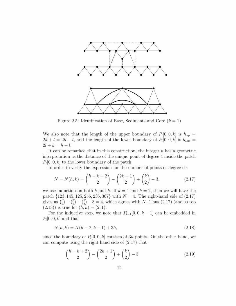
Figure 2.5: Identification of Base, Sediments and Core (k = 1)
We also note that the length of the upper boundary of Pl[0, 0, k] is hup =2k + l = 2h − l, and the length of the lower boundary of Pl[0, 0, k] is hlow =2l + k = h + l.
It can be remarked that in this construction, the integer k has a geometricinterpretation as the distance of the unique point of degree 4 inside the patchPl[0, 0, k] to the lower boundary of the patch.
In order to verify the expression for the number of points of degree six
N = N(h, k) =
(
h + k + 2
2
)
−
(
2k + 1
2
)
+
(
k
2
)
− 3, (2.17)
we use induction on both k and h. If k = 1 and h = 2, then we will have thepatch {123, 145, 125, 256, 236, 367} with N = 4. The right-hand side of (2.17)gives us
(
52
)
−(
32
)
+(
12
)
− 3 = 4, which agrees with N . Thus (2.17) (and so too(2.13)) is true for (h, k) = (2, 1).
For the inductive step, we note that Pl−1[0, 0, k − 1] can be embedded inPl[0, 0, k] and that
N(h, k) = N(h− 2, k − 1) + 3h, (2.18)
since the boundary of Pl[0, 0, k] consists of 3h points. On the other hand, wecan compute using the right hand side of (2.17) that
(
h+ k + 2
2
)
−
(
2k + 1
2
)
+
(
k
2
)
− 3 (2.19)
12

=
(
h+ k − 1
2
)
−
(
2k − 1
2
)
+
(
k − 1
2
)
− 3
+(3h+ 3k) − (4k − 1) + (k − 1)
=
(
h+ k − 1
2
)
−
(
2k − 1
2
)
+
(
k − 1
2
)
− 3 + 3h.
This verifies equation (2.17).
•SSSSSSSSSS •
kkkkkkkkkk
•
•
0000
00
������
•
@@@@
@@@@
~~~~
~~~~
•
0000
00
������
•<<
<<
����
•<<
<<
����
•<<
<<
����
•<<
<<
����
•<<
<<
����
•<<
<<
����
•<<
<<
����
• • • • • • • •
•
0000
00
������
•
@@@@
@@@@
~~~~
~~~~
•
0000
00
������
•<<
<<
����
•<<
<<
����
•<<
<<
����
•<<
<<
����
•<<
<<
����
•<<
<<
����
•<<
<<
����
• • • • • • • •
Figure 2.6: Identification of Top, Sediments and Core (k = 1, l = 3)
Assume that h > k ≥ l > 0. Then for each N of the form
N =
(
k + h+ l + 2
2
)
− 3
(
k + 1
2
)
− 3
(
l + 1
2
)
− 3,
it can be shown that there exists a patch with parameters (0, 3, 0, N)b withb = 3h, β4 = 1 which is of the form [0, l, k]. For the construction we firstassume that
l > max{2h− k − l, h+ k − 2l}. (2.20)
In this case we assemble the patch P [0, l, k]3h out of the following five parts:
C = P [0, 0, k − l]3(h−l); A = P [0, 0, 0]3(2h−k−l);
13

B = P [0, 0, 0]3(h+k−2l); Ql; R[0, 0, 0]6l.
Here R[0, 0, 0]6l is given by cutting off two smaller triangles P [0, 0, 0]3(2l+k−2h)
and P [0, 0, 0]3(3l−k−h) from the large triangle P [0, 0, 0]6l at two corners ofP [0, 0, 0]6l. That is,
R[0, 0, 0]6l := P [0, 0, 0]6l\(P [0, 0, 0]3(2l+k−2h)∪P [0, 0, 0]3(3l−k−h)). (2.21)
The boundary of the triangulation R[0, 0, 0]6l consists of altogether five edges,three of which are derived from the original boundary of the triangle P [0, 0, 0]6l,and the remaining two are new boundary edges. The part Ql is as defined in(2.16).
The left-hand side of the boundary of C = P [0, 0, k − l]3(h−l) is identifiedwith one side of the triangle A = P [0, 0, 0]3(2h−k−l); the right-hand side of theboundary of C is identified with one side of the triangle B = P [0, 0, 0]3(h+k−2l).The vertex of degree 4, that is, one of the meeting points of the left and right-hand side boundaries of C will be identified with the central point of degree4 of Ql. This point is also identified with one of the corners of the triangles Aand B. Parts of the boundaries of A and B are identified with the inner partsof the boundaries of Ql. This leaves three parts of the boundary of Ql withoutidentification, the top part which will be part of the boundary of the patch,and the two remaining inner parts Q ∩ R (refer to Figure 2.7). The centralpiece of the boundary of R[0, 0, 0]6l which is opposite to the corner point ofdegree four is identified with the union of the remaining two boundaries ofthe triangles A and B, namely, R ∩ (A ∪ B). The two new boundary parts ofR[0, 0, 0]6l are identified with the remaining inner parts of the boundary of Ql
as Q ∩ R (refer to Figure 2.7) and are easily seen to have the correspondinglengths 2l + k − 2h and 3l − k − h.
•
CA B
•
•
R
BBBBBBBBBBBBBBBBB
|||||||||||||||||
Q
Figure 2.7: Identification of five parts
14

By using parts (ii) and (iii) of Theorem 2.2.1, the number of points of degree6 of the parts C,A,B,Q,R can be seen to be as follows:
NA =
(
2h− k − l + 2
2
)
− 3 (2.22)
NB =
(
h+ k − 2l + 2
2
)
− 3 (2.23)
NC =
(
(h− l) + (k − l) + 2
2
)
−
(
2k − 2l + 1
2
)
+
(
k − l
2
)
− 3 (2.24)
NQ =
(
2l + 2
2
)
−
(
2l + 1
2
)
+
(
l
2
)
− 3 (2.25)
NR =
(
2l + 2
2
)
−
(
2l + k − 2h+ 1
2
)
−
(
3l − k − h+ 1
2
)
− 5 (2.26)
Note that the number of interior points of degree 6 in A,B are NA − 3(2h−k− l− 1), NB − 3(h+ k− 2l− 1), respectively. The number of interior pointsof degree 6 in C is NC − 3(h − l − 1) if k = l and NC − (3h − 3l − 2) ifk > l. The number of points of degree 6 in R except for those lying on thecommon boundary with Q, A, B is NR − 2l+3 whereas the number of pointsof degree 6 in Q except for those lying on the common boundary with R, A, Bis NQ−2(l−1). The number of points of degree 6 lying on each of the commonboundaries of R, A, B, C, Q are as follows:
N(R∩Q)l = 2l + k − 2h+ 1 (the left part of R ∩Q),
N(R∩Q)r = 3l − k − h + 1 (the right part of R ∩Q),
N(A∩R)\(R∩Q)l = 2h− k − l,
N(B∩R)\(A∩R)\(R∩Q)r = h+ k − 2l − 1,
N(A∩Q)\(A∩R) = 2h− k − l − 1,
N(B∩Q)\(A∩Q)\(B∩R) = h+ k − 2l − 1,
N(A∩C)\(A∩Q)\(A∩R) =
{
2h− k − l − 2, if k = l2h− k − l − 1, if k > l
,
N(B∩C)\(B∩Q)\(B∩R) = h+ k − 2l − 1.
Therefore the total number of points of degree 6 lying on the common bound-aries is
N =
{
6h− 4l − 4, if k = l6h− 4l − 3, if k > l
.
15

We also note that
2NA = (2h− k − l + 2)(2h− k − l + 1)− 6
= 4h2 + k2 + l2 − 4hk − 4hl + 2kl + 6h− 3k − 3l − 4,
2NB = (h+ k − 2l + 2)(h+ k − 2l + 1)− 6
= h2 + k2 + 4l2 + 2hk − 4hl − 4kl + 3h+ 3k − 6l − 4,
2NC = (h+ k − 2l + 2)(h+ k − 2l + 1)− (2k − 2l + 1)(2k − 2l)
+(k − l)(k − l − 1)− 6
= h2 − 2k2 + l2 + 2hk − 4hl + 2kl + 3h− 3l − 4,
2NQ = (2l + 2)(2l + 1)− 2l(2l + 1) + l(l − 1)− 6
= l2 + 3l − 4,
2NR = (2l + 2)(2l + 1)− (2l + k − 2h + 1)(2l + k − 2h)
−(3l − k − h+ 1)(3l − k − h)− 10
= −5h2 − 2k2 − 9l2 + 2hk + 14hl + 2kl + 3h+ l − 8.
It follows that for k = l, the number of points of degree 6 in this constructionis
N = (NA − 3(2h− k − l − 1)) + (NB − 3(h+ k − 2l − 1))
+(NC − 3(h− l − 1)) + (NR − 2l + 3)
+(NQ − 2(l − 1)) + N
=1
2(h2 − 2k2 − 2l2 + 2hk + 2hl + 2kl + 3h− 4).
If k > l, we also get the same N . Since(
h+ k + l + 2
2
)
− 3
(
k + 1
2
)
− 3
(
l + 1
2
)
− 3
=1
2[(h2 + hk + hl + h+ hk + k2 + kl + k + hl + kl + l2 + l
+2h+ 2k + 2l + 2)− (3k2 + 3k)− (3l2 + 3l)]− 3
=1
2(h2 − 2k2 − 2l2 + 2hk + 2hl + 2kl + 3h− 4),
we have the equality
N =
(
h+ k + l + 2
2
)
− 3
(
k + 1
2
)
− 3
(
l + 1
2
)
− 3. (2.27)
The various cases of smaller l, that is, those cases where (2.20) does nothold can be discussed in an analogous way.
16

Some preliminaries for the proof of Theorem 2.2.1
We remark that for any patch P with an interior point q ∈ P , the distanceof q to the boundary of P can be defined as the minimal number of trianglesthat are intersected by a topological path connecting q to the boundary of P.
If P is a patch such that all its boundary points have degree 6, with theexception of one point which has degree 4, then we may consider the union ofall triangles which are incident with the boundary of P. This union of triangles,as depicted in Figure 2.8 will be referred to as a belt around the patch.
•CCC
C{{{
{
•CCC
C{{{
{ •CCC
C{{{
{
•CCC
C{{{
{ •CCC
C{{{
{ •CCC
C{{{
{
•CCC
C •{{{
{ •CCC
C •{{{
{
•mmmmmmm •
QQQQQQQ
•QQQQQQQ •
mmmmmmm
•
•
1111
11
•mmmmmmm
1111
11 •
QQQQQQQ
• •
•
Figure 2.8: A belt around patch [o, l, k].
The following is an immediate consequence of our definitions.
Lemma 2.2.1 (i) If the boundary of the patch P and the interior of all thetriangles of a belt around P are removed, the remaining topological spaceis another (triangulated) patch P ′.
(ii) If q is an interior point of a patch P which has distance k to the boundary,then the distance of q to the boundary of P ′ is k − 1.
2.2.2 Proof of Theorem 2.2.1
Proof of part (i):
This is shown by induction on the number m = f1(P ) of points of the patchP . The theorem is true for m = 3, 6 since the patches with m = 3, 6 pointswhere three of the points have degree 4 are easily seen to be unique.
Assume that P is a patch of type (0, 3, 0, m− 3)b with m > 6 points. Fromthe description of the process of peeling the boundary, we may assume that the
17

boundary of the patch P contains a vertex point q of degree 4. Hence the pointq has precisely two adjacent points x, y which are both on the boundary of P .It is clear that d(x) = 4 or d(y) = 4 implies that m = 3, which contradictsour assumption that m > 6. Since the type of P is (0, 3, 0), it follows thatd(x) = d(y) = 6. Obviously xy is an interior edge of P, which is contained inthe triangle qxy, and so it must be contained in a second triangle xyz. Sinced(x) = d(y) = 6, it follows that the edges xz, yz are interior edges. There existtwo further points x′, y′ such that xx′, yy′ are boundary edges, which are thencontained in the triangles xx′z, yy′z respectively.
If the degree of z is d(z) = 4, then clearly x′y′ must be an edge on theboundary, and x′y′z must be a triangle. This implies that d(x′) = d(y′) = 5; acontradiction. Since P has parameters (0, 3, 0, m−3), it follows that d(z) = 6.This implies that x′ and y′ do not form an edge, and hence x′y′z is not atriangle.
y′
y
}}}}}}}}}}z
BBBB
BBBB
BBB
}}}}
}}}}
}}• P
′
q x
x′
Figure 2.9: Cutting the corner at q.
By cutting the corner at q, as explained in Section 2.9 (see Figure ??), wereplace the four triangles qxy, xx′z, yy′z, xyz by a single triangle x′y′z, therebyremoving the three points q, x, y and obtaining a patch P ′ which has d(z) = 4.Note that in P ′ the points x′, y′ are boundary points, but z is an interior point.Observe that the number of points, and the length of the boundaries of P andP ′ are related by the equations:
b′ = b− 3, m′ = m− 3. (2.28)
Since the number of vertex points of P ′ is m′ = m− 3 < m, it follows fromthe hypothesis of the induction that the length of the boundary b′ of the patchP ′ is a multiple of 3, that is, b′ = 3h′ for some positive integer h′. By (2.28)we see that the number b = 3 + 3h′ = 3(h′ + 1) is also a multiple of 3. Thisproves the first part of the theorem.
18

The existence of patches of the types mentioned in parts (ii), (iii) and (iv)of Theorem 2.2.1 have already been shown in Section 2.2.1. We are thus leftwith the task of showing the necessity part.
Proof of part (ii):
We prove the necessity part of part (ii) by induction on the boundary lengthb = 3h. The statement (ii) is clearly true for h = 1, since the only patch withboundary length 3 is a triangle.
Assume that the statement (ii) is true for any h′ < h. Let P be a patch withparameters (0, 3, 0, N)3h with β4 = 3, so that the boundary length is 3h > 1.
Take any pair x, y of the three boundary points of degree 4, and considerthat part of the boundary between them which does not contain the thirdpoint of degree 4. Assume that h1 is the length of this part of the boundary,which means that that part of the boundary has h1 edges and h1 + 1 vertexpoints. The lengths of the other two parts of the boundary between the pointsof degree four are denoted by h2, h3. Hence the overall length of the boundaryof the given patch is b = h1 + h2 + h3. By assumption, all inner points on thisboundary (that is, the points on the boundary other than the three of degree4) as well as the points inside the patch at distance one from this boundarypart must have degree 6. The segment x′y′ connecting the h1 points of degreesix which are of distance one from the boundary part of length h1 separatesthe boundary from the rest of the triangle, and the area between the boundaryand this segment consists of a strip of 2h1 − 1 triangles (refer to Figure 2.10).
By removing this strip from the patch, we obtain a smaller patch P ′ whichhas three boundary segments of lengths h1−1, h2−1, h3−1, and also containsthree boundary points of degree 4 on its boundary, namely, the third originalboundary point, and the two end points x′, y′. Hence the overall length of theboundary of P ′ is (using part (i))
3h′ = (h1 − 1) + (h2 − 1) + (h3 − 1) = h1 + h2 + h3 − 3 = b− 3.
By the inductive assumption, we have that
h1 − 1 = h2 − 1 = h3 − 1,
and hence h1 = h2 = h3. We denote this common quantity by h = hi.
19

•
h3−1
DD
DD
DD
DD
h2−1
yy
yy
yy
yy
x′
����
�==
=== •
����
��;;
;;;; •
����
��;;
;;;; y′
����
�==
===
x •h1
• • y
Figure 2.10: A strip of 2h1 − 1 triangles
Again by the inductive assumption, we see that for the patch P ′ with pa-rameters (0, 3, 0, N ′)3h′, we get for N ′ the equation
N ′ =
(
(h− 1) + 2
2
)
− 3.
Hence the total number of vertex points of degree 6 in P is
N = N ′ + (h1 + 1) =
(
(h− 1) + 2
2
)
− 3 + h+ 1 =
(
h+ 2
2
)
− 3.
This completes the proof of part (ii).
Proof of part (iii):
For the proof of (iii) we use induction on the integer l > 0. We may assumethroughout that k > 0. That is, one of the points of degree four is not on theboundary of the patch. Let x, y be the two boundary points of degree four, andassume that hl, hu are the lengths of the two boundary parts between x and y,that is, the number of edges of the two parts of the boundary between x and y.The triangles which are next to the boundary form a strip (refer to Figure 2.11)consisting of 2hl−1 or 2hu−1 triangles. After removing one of these strips fromthe patch, we get another patch of the kind [0, 0, k] or [0, 0, k−1], depending onwhich strip is removed. We choose the notation in such a way that removingthe boundary segment with hl edges gives rise to the remaining patch P ′ ofthe form [0, 0, k]. In this case we get two new points x′, y′ on the boundary ofP ′, which are of degree four. It is clear that removing the strip reduces thetotal boundary length by 3, hence we have b′ = b−3, that is, h′ = h−1. Fromk′ = k it follows that l′ = l − 1. Note that by the induction assumption of(iii), we get h′
l = 2h′ − l′ = 2h− 2 − l + 1 = 2h− l − 1. From Figure 2.11 we
20

easily infer that hl = h′l +1, that is, we have hl = 2h− l = h+ k. Clearly, this
implies that hu = 3h− hl = h+ l. Now we may use the inductive assumptionfor the formula on the number N ′ to complete the proof, remembering that inthe original patch, the points x′, y′ have degree 6 whereas the points x, y havedegree 4. Then
N = (hl + 1) +N ′
= (hl + 1) +
(
h′ + k′ + 2
2
)
−
(
2k′ + 1
2
)
+
(
k′
2
)
− 3
= (h+ k + 1) +
(
(h− 1) + k + 2
2
)
−
(
2k + 1
2
)
+
(
k
2
)
− 3
=
(
h + k + 2
2
)
−
(
2k + 1
2
)
+
(
k
2
)
− 3.
This completes the proof of part (iii).
•
DD
DD
DD
DD
yy
yy
yy
yy
x′
����
�==
=== •
����
��;;
;;;; •
����
��;;
;;;; y′
����
�==
===
x •h1
• • y
Figure 2.11: A strip of triangles.
Proof of part (iv):
Again we use induction on l > 0. Let P be a patch with parameters (0, 3, 0, N)3hwith β4 = 1 and of the form [0, l, k] where 0 < l ≤ k < h. If we remove alltriangles which are incident with the boundary from P , then we obtain a belt(refer to Figure 2.8) consisting of 2b−3 triangles. Removing this belt from P ,we obtain another patch P ′ of the form [0, l− 1, k − 1] which is easily seen tohave the boundary length b′ = b− 3.
By the induction assumption we have that the number of points of degree6 in P ′ is
N ′ =
(
h′ + k′ + l′ + 2
2
)
− 3
(
k′ + 1
2
)
− 3
(
l′ + 1
2
)
− 3.
21

Note that h′ = h− 1, l′ = l− 1, k′ = k − 1. Taking into consideration the factthat the boundary of P has one point of degree 4 and all other points of degree6, we obtain for the total number of points of degree 6 in P the expression
N = (N ′ + 1) + (b− 1)
= N ′ + 3h
= 3h+
(
h′ + k′ + l′ + 2
2
)
− 3
(
k′ + 1
2
)
− 3
(
l′ + 1
2
)
− 3
= 3h+
(
h+ k + l − 1
2
)
− 3
(
k
2
)
− 3
(
l
2
)
− 3
=
(
h + k + l + 2
2
)
− 3
(
k + 1
2
)
− 3
(
l + 1
2
)
− 3
This completes the proof of (iv).
2.3 Construction of certain patches
of types (0, 2, 2), (0, 1, 4), (0, 0, 6)
As a consequence of the above constructions, we can also construct certainpatches of types (0, 2, 2), (0, 1, 4) and (0, 0, 6). As defined earlier on, we let β5
be the number of points of degree 5 which are on the boundary. In this sectionwe only consider the following kinds of patches:
(i) (0, 2, 2) with β5 = 2;
(ii) (0, 1, 4) with β5 = 4;
(iii) (0, 0, 6) with β5 = 6.
2.3.1 Type (1): (0, 2, 2, N)b′ with β5 = 2 and β4 = 2.
We can construct this type from patches with parameters (0, 3, 0, N)3h, withβ4 = 3, of type Ph[0, 0, 0]. Here we take a patch of type Ph[0, 0, 0], remove asubpatch of type Pc−1[0, 0, 0] (2 ≤ c ≤ h) which contains one of the boundarypoints of degree four, and take the topological closure to obtain a new patchP ′ of type (0, 2, 2). The edge-distance between the two boundary points ofdegree five in P ′ is c− 1, and the edge-distance between a boundary point ofdegree four and one of degree five is h− c+ 1. The length of the boundary of
22

P ′ is b′ = (c− 1) + 2(h− c + 1) + h = 3h− c + 1. By Theorem 2.2.1(ii), thenumber of vertex points of degree 6 in Ph[0, 0, 0] and Pc−1[0, 0, 0] are
N =
(
h+ 2
2
)
− 3
and
Nc−1 =
(
(c− 1) + 2
2
)
− 3 =
(
c+ 1
2
)
− 3,
respectively. Therefore the number of vertex points of degree 6 in P ′ is
N = N −Nc−1 + (c− 2)− 2 =
(
h + 2
2
)
−
(
c
2
)
− 4.
2.3.2 Type (2): (0, 2, 2, N)b′ with β5 = 2 and β4 = 1.
We can construct this type from the patch with parameters (0, 3, 0, N)3h, withβ4 = 2, of type [0, 0, k]. Here we take a patch of type Ph−k[0, 0, k], remove asubpatch of type Pc−1[0, 0, 0] (c ≤ h−k+1) which contains one of the boundarypoints of degree four, and take the topological closure to obtain a new patchP ′ of type (0, 2, 2). Here c−1 is the number of edges on the boundary betweenthe boundary point of degree four on Ph−k[0, 0, k] and (either of) the boundarypoints of degree five of the new patch P ′. The length of the boundary of P ′ isb′ = 3h− c+1. The edge-distance between the two boundary points of degreefive is c − 1. By Theorem 2.2.1, the number of vertex points of degree 6 inPh−k[0, 0, k] and Pc−1[0, 0, 0] are
N =
(
h+ k + 2
2
)
−
(
2k + 1
2
)
+
(
k
2
)
− 3
and
Nc−1 =
(
(c− 1) + 2
2
)
− 3 =
(
c+ 1
2
)
− 3,
respectively. Therefore the number of vertex points of degree 6 in P ′ is
N = N −Nc−1 + (c− 2)− 2
=
(
h + k + 2
2
)
−
(
2k + 1
2
)
+
(
k
2
)
−
(
c
2
)
− 4.
23

2.3.3 Type (3): (0, 2, 2, N)b′ with β5 = 2 and β4 = 0.
We can construct this type from the patch with parameters (0, 3, 0, N)3h, withβ4 = 1, of type [0, l, k]. Here we take a patch of type P [0, l, k]3h, remove asubpatch of type Pc−1[0, 0, 0] (c ≤ h + 1) which contains one of the boundarypoints of degree four, and take the topological closure to obtain a new patchP ′ of type (0, 2, 2). Here c−1 is the number of edges on the boundary betweenthe boundary point of degree four on P [0, l, k]3h and (either of) the boundarypoints of degree five of the new patch P ′. The length of the boundary of P ′ isb′ = 3h− c+1. The edge-distance between the two boundary points of degreefive is c − 1. By Theorem 2.2.1, the number of vertex points of degree 6 inP [0, l, k]3h and Pc−1[0, 0, 0] are
N =
(
h + k + l + 2
2
)
− 3
(
k + 1
2
)
− 3
(
l + 1
2
)
− 3
and
Nc−1 =
(
c+ 1
2
)
− 3,
respectively. Therefore the number of vertex points of degree 6 in P ′ is
N = N −Nc−1 + (c− 2)− 2
=
(
h + k + l + 2
2
)
− 3
(
k + 1
2
)
− 3
(
l + 1
2
)
−
(
c
2
)
− 4.
2.3.4 Type (4): (0, 1, 4, N)b′ with β5 = 4 and β4 = 1.
We can construct this type from patches with parameters (0, 3, 0, N)3h, withβ4 = 3, of type Ph[0, 0, 0]. Here we take a patch of type Ph[0, 0, 0], removetwo subpatches of types Pc1−1[0, 0, 0], Pc2−1[0, 0, 0], each of which contains aboundary point of Ph[0, 0, 0] of degree four, and take the topological closureto obtain a new patch P ′ of type (0, 1, 4). Clearly we must have (c1 − 1) +(c2− 1) < h. By Theorem 2.2.1(ii), the number of vertex points of degree 6 inPh[0, 0, 0], Pc1−1[0, 0, 0] and Pc2−1[0, 0, 0] are
N =
(
h + 2
2
)
− 3,
Nc1−1 =
(
(c1 − 1) + 2
2
)
− 3 =
(
c1 + 1
2
)
− 3
24

and
Nc2−1 =
(
(c2 − 1) + 2
2
)
− 3 =
(
c2 + 1
2
)
− 3,
respectively. Therefore the number of vertex points of degree 6 in P ′ is
N = N −Nc1−1 −Nc2−1 + (c1 − 2)− 2 + (c2 − 2)− 2
=
(
h + 2
2
)
−
(
c12
)
−
(
c22
)
− 5.
Note that in the case c1+ c2− 2 = h, there is another kind of patch of type(0, 2, 2). This will be discussed below as type (7).
2.3.5 Type (5): (0, 1, 4, N)b′ with β5 = 4 and β4 = 0.
We can construct this type from patches with parameters (0, 3, 0, N)3h, withβ4 = 2, of type [0, 0, k]. Here we take a patch of type Ph−k[0, 0, k], remove twosubpatches of types Pc1−1[0, 0, 0] and Pc2−1[0, 0, 0], each of which contains oneof the boundary points of Ph−k[0, 0, k] of degree four, and take the topologicalclosure to obtain a new patch P ′ of type (0, 1, 4). Clearly we must have(c1 − 1) + (c2 − 1) < h. By Theorem 2.2.1, the number of vertex points ofdegree 6 in Ph−k[0, 0, k], Pc1−1[0, 0, 0] and Pc2−1[0, 0, 0] are
N =
(
h+ k + 2
2
)
−
(
2k + 1
2
)
+
(
k
2
)
− 3,
Nc1−1 =
(
(c1 − 1) + 2
2
)
− 3 =
(
c1 + 1
2
)
− 3
and
Nc2−1 =
(
(c2 − 1) + 2
2
)
− 3 =
(
c2 + 1
2
)
− 3,
respectively. Therefore the number of vertex points of degree 6 in P ′ is
N = N −Nc1−1 −Nc2−1 + (c1 − 2)− 2 + (c2 − 2)− 2
=
(
h + k + 2
2
)
−
(
2k + 1
2
)
+
(
k
2
)
−
(
c12
)
−
(
c22
)
− 5.
25

2.3.6 Type (6): (0, 0, 6, N)b′ with β5 = 6 and β4 = 0.
We can construct this type from patches with parameters (0, 3, 0, N)3h, withβ4 = 3, of type Ph[0, 0, 0]. Here we take a patch of type Ph[0, 0, 0], removethree subpatches of type Pc1−1[0, 0, 0], Pc2−1[0, 0, 0], Pc3−1[0, 0, 0], each of whichcontains one of the boundary points Ph[0, 0, 0, ] of degree four, and take thetopological closure to obtain a new patch P ′ of type (0, 6, 6). Clearly we musthave c1 + c2 − 2 < h, c1 + c3 − 2 < h, c2 + c3 − 2 < h. By Theorem 2.2.1, thenumber of vertex points of degree 6 in Ph[0, 0, k], Pc1−1[0, 0, 0], Pc2−1[0, 0, 0]and Pc3−1[0, 0, 0] are
N =
(
h + 2
2
)
− 3,
Nc1−1 =
(
(c1 − 1) + 2
2
)
− 3 =
(
c1 + 1
2
)
− 3,
Nc2−1 =
(
(c2 − 1) + 2
2
)
− 3 =
(
c2 + 1
2
)
− 3,
and
Nc3−1 =
(
(c3 − 1) + 2
2
)
− 3 =
(
c3 + 1
2
)
− 3,
respectively. Therefore the number of vertex points of degree 6 in P ′ is
N = N −Nc1−1 −Nc2−1 −Nc3−1 + (c1 − 2)− 2 + (c2 − 2)− 2
+(c3 − 2)− 2
=
(
h + 2
2
)
−
(
c12
)
−
(
c22
)
−
(
c32
)
− 6.
2.3.7 Type (7): (0, 2, 2, N)b′ with β5 = 2 and β4 = 2.
In contrast to type (1), the boundary points of degree 4 and 5 are arranged incyclic order at the corners as 4, 5, 4, 5.
This type can be constructed by glueing u reduced strips (refer to Figure2.12) consisting of 2v triangles.
26

•
////
///
������� •
////
///
������� •
////
///
������� •
�������
• •u=1,v=3
• •
•
////
///
������� •
////
///
������� •
////
///
������� •
�������
•
////
///
������� •
////
///
������� •
////
///
������� •
�������
• •u=2,v=3
• •
Figure 2.12: Patch with corner points 4, 5, 4, 5
2.4 Some applications towards the classifica-
tion of patches
We first consider patches of Type (1), that is, (0, 2, 2, m)b′ with β5 = 2 andβ4 = 2. Let us additionally assume that the four boundary points of degreeless than six are arranged in cyclic order such that the two points of degree 4precede the two points of degree 5 (refer to Figure 2.13).
Let us choose positive integers s, t, c, h such that the two points of degree 5are the end points of a boundary string of c− 1 edges, and such that the twopoints of degree 4 are the end points of a string of h edges. Let us assume thatthe remaining two pieces of the boundary between the two pairs of points ofdegrees 4 and 5 have lengths s and t (refer to Figure 2.13).
5
s
}}}}
}}}}
}}}}
c−15
t
AAAA
AAAA
AAAA
4h
4
Figure 2.13: Patch with corner points 4, 4, 5, 5.
Theorem 2.4.1 Under the assumptions on a patch P with arrangement ofboundary points 4, 4, 5, 5, and lengths as in Figure 2.13 (as stated in the pre-vious paragraph), we have the following:
(i) s = t;
(ii) c− 1 + s = h;
(iii) h ≥ c;
27
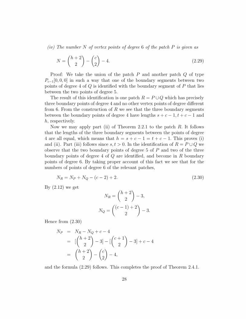
(iv) The number N of vertex points of degree 6 of the patch P is given as
N =
(
h+ 2
2
)
−
(
c
2
)
− 4. (2.29)
Proof: We take the union of the patch P and another patch Q of typePc−1[0, 0, 0] in such a way that one of the boundary segments between twopoints of degree 4 of Q is identified with the boundary segment of P that liesbetween the two points of degree 5.
The result of this identification is one patch R = P ∪Q which has preciselythree boundary points of degree 4 and no other vertex points of degree differentfrom 6. From the construction of R we see that the three boundary segmentsbetween the boundary points of degree 4 have lengths s+ c− 1, t+ c− 1 andh, respectively.
Now we may apply part (ii) of Theorem 2.2.1 to the patch R. It followsthat the lengths of the three boundary segments between the points of degree4 are all equal, which means that h = s + c − 1 = t + c − 1. This proves (i)and (ii). Part (iii) follows since s, t > 0. In the identification of R = P ∪Q weobserve that the two boundary points of degree 5 of P and two of the threeboundary points of degree 4 of Q are identified, and become in R boundarypoints of degree 6. By taking proper account of this fact we see that for thenumbers of points of degree 6 of the relevant patches,
NR = NP +NQ − (c− 2) + 2. (2.30)
By (2.12) we get
NR =
(
h+ 2
2
)
− 3,
NQ =
(
(c− 1) + 2
2
)
− 3.
Hence from (2.30)
NP = NR −NQ + c− 4
= [
(
h+ 2
2
)
− 3]− [
(
c+ 1
2
)
− 3] + c− 4
=
(
h+ 2
2
)
−
(
c
2
)
− 4,
and the formula (2.29) follows. This completes the proof of Theorem 2.4.1.
28

In the case of Type (2), that is, (0, 2, 2, m)b′ with β5 = 2 and β4 = 1, let uschoose positive integers s, t, c such that the two points of degree 5 are the endpoints of a boundary string of c− 1 edges and such that the boundary pointof degree 4 is one end point of two strings of s, t edges with second endpointof degree 5 (refer to Figure 2.14).
4
s
����
������
����
���
t
2222
2222
2222
2222
2
5c−1
5
Figure 2.14: Patch with boundary points 4, 5, 5
Theorem 2.4.2 Under the assumptions on a patch P of type (0, 2, 2, m)b′
with the lengths of the boundary segments as in Figure 2.14 (as stated in theprevious paragraph), we have the following:
(i) s+ t+ 2(c− 1), 2s− t+ (c− 1), 2t− s+ (c− 1) are multiples of 3;
(ii) There exist integers h, k, l such that
h =1
3(s+ t + 2(c− 1)), (2.31)
k =1
3(2s− t+ (c− 1)), (2.32)
l =1
3(2t− s+ (c− 1)), (2.33)
and such that the patch P has precisely
N =
(
h+ k + 2
2
)
−
(
2k + 1
2
)
+
(
k
2
)
−
(
c
2
)
− 4 (2.34)
vertex points of degree 6.
Proof: We take the union of the patch P and another patch Q of typePc−1[0, 0, 0] in such a way that one of the boundary segments between two
29

points of degree 4 of Q is identified with the boundary segment of P that liesbetween the two points of degree 5.
The result of this identification is one patch R = P ∪Q which has preciselytwo boundary points of degree 4, and it contains precisely one point of degree4 in its interior, since by assumption P ⊂ R is of type (0, 2, 2, m). Hence Ris a patch of type (0, 3, 0) with β4 = 2. We see that the total length of theboundary of R is s + t + 2(c − 1). By Theorem 2.2.1(i) it follows that thisboundary length is a multiple of 3. From
2t− s + (c− 1) = 3(t+ c− 1)− (s+ t + 2(c− 1)),
2s− t + (c− 1) = 3(s+ c− 1)− (s+ t+ 2(c− 1)),
it follows that the other two integers 2t− s+ (c− 1), 2s− t+ (c− 1) are alsomultiples of 3.
In the identification of R = P ∪Q we observe that the two boundary pointsof degree 5 of P and two of the three boundary points of degree 4 of Q areidentified, and become in R boundary points of degree 6. By taking properaccount of this fact we see that for the numbers of points of degree 6 of therelevant patches,
NR = NP +NQ − (c− 2) + 2. (2.35)
By referring to Figure 2.14 we see that the lengths of the two boundary seg-ments between the two boundary points of degree 4 are given as s+ c− 1 andt+ c− 1. By using part (iii) of Theorem 2.2.1 we may take
h+ l = t+ c− 1,
2h− l = s+ c− 1.
By adding these two equations we see that 3h = s+t+2(c−1). By subtractingthe second equation from twice the first we have that 3l = 2t−s+ c−1. Fromthe fact that k + l = h (by Theorem 2.2.1(iii)), we have
k =1
3(2s− t+ c− 1). (2.36)
By (2.13) we get
NR =
(
h + k + 2
2
)
−
(
2k + 1
2
)
+
(
k
2
)
− 3,
30

and by (2.12) we have
NQ =
(
(c− 1) + 2
2
)
− 3.
Hence from (2.35)
NP = NR −NQ + c− 4
= [
(
h+ k + 2
2
)
−
(
2k + 1
2
)
+
(
k
2
)
− 3]
−[
(
c+ 1
2
)
− 3] + c− 4
=
(
h+ k + 2
2
)
−
(
2k + 1
2
)
+
(
k
2
)
−
(
c
2
)
− 4,
and the formula (2.34) follows. This completes the proof of Theorem 2.4.2.
In the case of Type (3), that is, (0, 2, 2, m)b′ with β5 = 2 and β4 = 0, let uschoose positive integers s, c such that the two points of degree 5 are the endpoints of two boundary strings with c− 1 and s edges (refer to Figure 2.15).
5
s
5
c−1
Figure 2.15: Boundary of a patch with two boundary points of degree 5
Theorem 2.4.3 Under the assumptions on a patch P of type (0, 2, 2, m)b′
with the lengths of the boundary segments as in Figure 2.15 (as stated in theprevious paragraph), we have the following:
(i) s+ 2(c− 1), 2s+ (c− 1) are multiples of 3;
(ii) There exist integers h, k, l such that
h =1
3(s+ 2(c− 1)) (2.37)
31

and such that the patch P has precisely
N =
(
h+ k + l + 2
2
)
− 3
(
k + l
2
)
− 3
(
l + 1
2
)
−
(
c
2
)
− 4 (2.38)
vertex points of degree 6.
Proof: We take the union of the patch P and another patch Q of typePc−1[0, 0, 0] in such a way that one of the boundary segments between twopoints of degree 4 of Q is identified with the boundary segment of P that liesbetween the two points of degree 5 that contains c− 1 edges.
The result of this identification is one patch R = P ∪Q which has preciselyone boundary point of degree 4, and it contains precisely two points of degree4 in its interior, since by assumption P ⊂ R is of type (0, 2, 2, m). Hence Ris a patch of type (0, 3, 0) with β4 = 1. We see that the total length of theboundary of R is s+2(c−1). By Theorem 2.2.1(i) it follows that this boundarylength is a multiple of 3. That is, s+ 2(c− 1) = 3h for some integer h. From
2s+ (c− 1) = 3(s+ c− 1)− (s+ 2(c− 1)),
it follows that 2s+ (c− 1) is also a multiple of 3.In the identification of R = P ∪Q we observe that the two boundary points
of degree 5 of P and two of the three boundary points of degree 4 of Q areidentified, and become in R boundary points of degree 6. By taking properaccount of this fact we see that for the numbers of points of degree 6 of therelevant patches,
NR = NP +NQ − (c− 2) + 2. (2.39)
By part (iv) of Theorem 2.2.1 we see that there exist integers k, l where 0 <l ≤ k < h such that
NR =
(
h+ k + l + 2
2
)
− 3
(
k + l
2
)
− 3
(
l + 1
2
)
− 3.
By Theorem 2.2.1(ii),
NQ =
(
(c− 1) + 2
2
)
− 3.
32

Hence from (2.39)
NP = NR −NQ + c− 4
= [
(
h+ k + l + 2
2
)
− 3
(
k + l
2
)
− 3
(
l + 1
2
)
− 3]− [
(
c+ 1
2
)
− 3]
+c− 4
=
(
h+ k + l + 2
2
)
− 3
(
k + l
2
)
− 3
(
l + 1
2
)
−
(
c
2
)
− 4,
and the formula (2.38) follows. This completes the proof of Theorem 2.4.3.
In the case of Type (4), that is, (0, 1, 4, m)b′ with β5 = 4 and β4 = 1, letus choose positive integers r, s, t, c1, c2 such that the four points of degree 5are the end points of three boundary strings with c1 − 1, r, c2− 1 edges in thiscyclic order respectively (refer to Figure 2.16) and such that the two segmentsof the boundary containing the boundary point of degree 4 have s and t edgesrespectively (refer to Figure 2.16).
4t
GGGGGGGGGGGG
s
wwwwwwwwwwww
5
c1−1
5
c2−1
5 r 4
Figure 2.16: Boundary of a patch with four boundary points of degree 5, oneof degree 4.
Theorem 2.4.4 Under the assumptions on a patch P of type (0, 1, 4, m)b′with the lengths of the boundary segments as in Figure 2.16 (as stated in theprevious paragraph), we have the following:
(i) The integer r + s+ t+ 2(c1 − 1) + 2(c2 − 1) is a multiple of 3;
(ii) The equality
s+ c1 − 1 = t+ c2 − 1 = r + c1 + c2 − 2 (2.40)
holds;
33

(iii) The patch P has precisely
N =
(
h+ 2
2
)
−
(
c12
)
−
(
c22
)
− 5 (2.41)
vertex points of degree 6 where h = s+ c1 − 1.
Proof: We take the union of the patch P and two more patches Q1, Q2
of types Pc1−1[0, 0, 0], Pc2−1[0, 0, 0] respectively in such a way that one of theboundary segments between two points of degree 4 of Qi is identified with theboundary segment of P that lies between the two points of degree 5 whichcontain ci − 1 edges (i = 1, 2).
The result of this identification is one patch R = P ∪ Q1 ∪ Q2 which hasprecisely three boundary points of degree 4. Hence R is a patch of type (0, 3, 0)with β4 = 3. We see that the total length of the boundary of R is r + s+ t +2(c1− 1)+ 2(c2− 1). By Theorem 2.2.1(i) it follows that this boundary lengthis a multiple of 3.
In the identification of R = P ∪Q1∪Q2 we observe that the four boundarypoints of degree 5 of P and two of the three boundary points of degree 4 ofQ1, Q2 each are identified, and become in R boundary points of degree 6. Bytaking proper account of this fact we see that for the numbers of points ofdegree 6 of the relevant patches,
NR = NP +NQ1+NQ2
− (c1 − 2)− (c2 − 2) + 4. (2.42)
By Theorem 2.2.1(ii) we see that all three boundary parts of R between theboundary points of degree 4 are equal, that is,
s+ c1 − 1 = t + c2 − 1 = r + c1 − 1 + c2 − 1 = h,
which proves part (ii).For the number of vertex points of degree 6 of the patch R we see from
Theorem 2.2.1(ii) that
NR =
(
h+ 2
2
)
− 3.
We also have by Theorem 2.2.1(ii) that
NQ1=
(
(c1 − 1) + 2
2
)
− 3, NQ2=
(
(c2 − 1) + 2
2
)
− 3.
34

Hence from (2.42)
NP = NR −NQ1−NQ2
+ c1 + c2 − 8
= [
(
h+ 2
2
)
− 3]
−[
(
c1 + 1
2
)
− 3]− [
(
c2 + 1
2
)
− 3] + c1 + c2 − 8
=
(
h+ 2
2
)
−
(
c12
)
−
(
c22
)
− 5,
and the formula (2.41) follows. This completes the proof of Theorem 2.4.4.
In the case of Type (5), that is, (0, 1, 4, m)b′ with β5 = 4 and β4 = 0, let uschoose positive integers s, t, c1, c2 such that the four points of degree 5 are theend points of four boundary strings with s, c1 − 1, t, c2 − 1 edges in this cyclicorder respectively (refer to Figure 2.17).
5
c1−1
s5
c2−1
5t
5
Figure 2.17: Boundary of a patch with four boundary points of degree 5.
Theorem 2.4.5 Under the assumptions on a patch P of type (0, 1, 4, m)b′
with the lengths of the boundary segments as in Figure 2.17 (as stated in theprevious paragraph), we have the following:
(i) The integers
s+t+2(c1−1)+2(c2−1), 2s−t+(c1−1)+(c2−1), 2t−s+(c1−1)+(c2−1)
are multiples of 3;
(ii) There exist integers h, k, l such that
h =1
3(s+ t + 2(c1 − 1) + 2(c2 − 1)), (2.43)
k =1
3(2s− t+ (c1 − 1) + (c2 − 1)), (2.44)
l =1
3(2t− s+ (c1 − 1) + (c2 − 1)), (2.45)
35
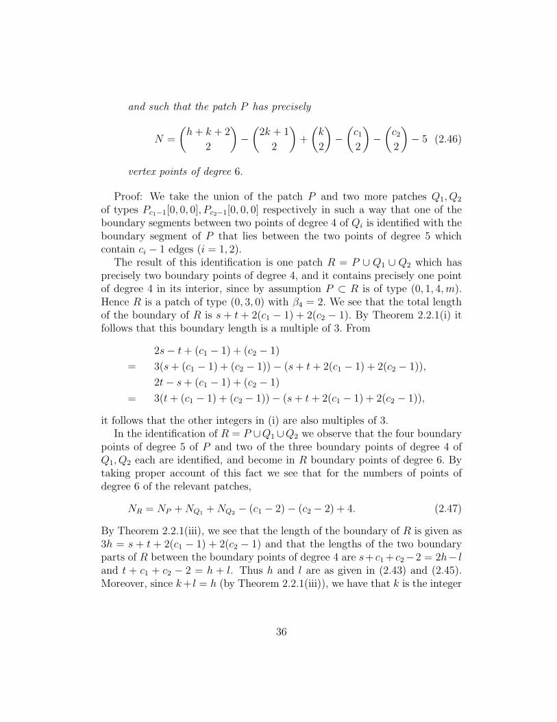
and such that the patch P has precisely
N =
(
h+ k + 2
2
)
−
(
2k + 1
2
)
+
(
k
2
)
−
(
c12
)
−
(
c22
)
− 5 (2.46)
vertex points of degree 6.
Proof: We take the union of the patch P and two more patches Q1, Q2
of types Pc1−1[0, 0, 0], Pc2−1[0, 0, 0] respectively in such a way that one of theboundary segments between two points of degree 4 of Qi is identified with theboundary segment of P that lies between the two points of degree 5 whichcontain ci − 1 edges (i = 1, 2).
The result of this identification is one patch R = P ∪ Q1 ∪ Q2 which hasprecisely two boundary points of degree 4, and it contains precisely one pointof degree 4 in its interior, since by assumption P ⊂ R is of type (0, 1, 4, m).Hence R is a patch of type (0, 3, 0) with β4 = 2. We see that the total lengthof the boundary of R is s + t + 2(c1 − 1) + 2(c2 − 1). By Theorem 2.2.1(i) itfollows that this boundary length is a multiple of 3. From
2s− t+ (c1 − 1) + (c2 − 1)
= 3(s+ (c1 − 1) + (c2 − 1))− (s+ t+ 2(c1 − 1) + 2(c2 − 1)),
2t− s+ (c1 − 1) + (c2 − 1)
= 3(t+ (c1 − 1) + (c2 − 1))− (s+ t + 2(c1 − 1) + 2(c2 − 1)),
it follows that the other integers in (i) are also multiples of 3.In the identification of R = P ∪Q1∪Q2 we observe that the four boundary
points of degree 5 of P and two of the three boundary points of degree 4 ofQ1, Q2 each are identified, and become in R boundary points of degree 6. Bytaking proper account of this fact we see that for the numbers of points ofdegree 6 of the relevant patches,
NR = NP +NQ1+NQ2
− (c1 − 2)− (c2 − 2) + 4. (2.47)
By Theorem 2.2.1(iii), we see that the length of the boundary of R is given as3h = s + t + 2(c1 − 1) + 2(c2 − 1) and that the lengths of the two boundaryparts of R between the boundary points of degree 4 are s+ c1+ c2−2 = 2h− land t + c1 + c2 − 2 = h + l. Thus h and l are as given in (2.43) and (2.45).Moreover, since k+ l = h (by Theorem 2.2.1(iii)), we have that k is the integer
36
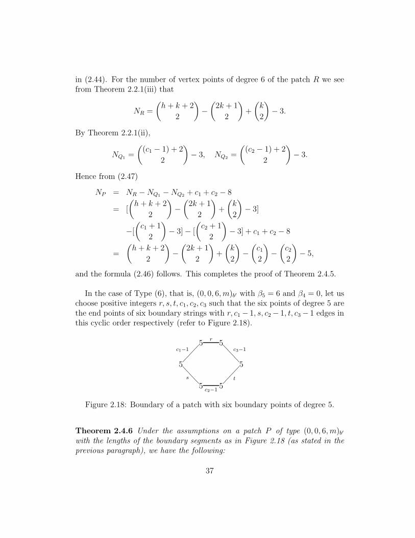
in (2.44). For the number of vertex points of degree 6 of the patch R we seefrom Theorem 2.2.1(iii) that
NR =
(
h + k + 2
2
)
−
(
2k + 1
2
)
+
(
k
2
)
− 3.
By Theorem 2.2.1(ii),
NQ1=
(
(c1 − 1) + 2
2
)
− 3, NQ2=
(
(c2 − 1) + 2
2
)
− 3.
Hence from (2.47)
NP = NR −NQ1−NQ2
+ c1 + c2 − 8
= [
(
h+ k + 2
2
)
−
(
2k + 1
2
)
+
(
k
2
)
− 3]
−[
(
c1 + 1
2
)
− 3]− [
(
c2 + 1
2
)
− 3] + c1 + c2 − 8
=
(
h+ k + 2
2
)
−
(
2k + 1
2
)
+
(
k
2
)
−
(
c12
)
−
(
c22
)
− 5,
and the formula (2.46) follows. This completes the proof of Theorem 2.4.5.
In the case of Type (6), that is, (0, 0, 6, m)b′ with β5 = 6 and β4 = 0, let uschoose positive integers r, s, t, c1, c2, c3 such that the six points of degree 5 arethe end points of six boundary strings with r, c1 − 1, s, c2− 1, t, c3− 1 edges inthis cyclic order respectively (refer to Figure 2.18).
5c1−1
����
���
r5
c3−1
====
===
5
s ====
=== 5
t��
����
�
5c2−1
5
Figure 2.18: Boundary of a patch with six boundary points of degree 5.
Theorem 2.4.6 Under the assumptions on a patch P of type (0, 0, 6, m)b′
with the lengths of the boundary segments as in Figure 2.18 (as stated in theprevious paragraph), we have the following:
37

(i) The integer r+ s+ t+ 2(c1 − 1) + 2(c2 − 1) + 2(c3 − 1) is a multiple of 3;
(ii) The equality
r + c1 + c3 − 2 = s+ c1 + c2 − 2 = t+ c2 + c3 − 2 (2.48)
holds;
(iii) The patch P has precisely
N =
(
h+ 2
2
)
−
(
c12
)
−
(
c22
)
−
(
c32
)
− 6 (2.49)
vertex points of degree 6 where h = r + c1 + c3 − 2.
Proof: We take the union of the patch P and three more patches Q1, Q2, Q3
of types Pc1−1[0, 0, 0], Pc2−1[0, 0, 0], Pc3−1[0, 0, 0] respectively in such a way thatone of the boundary segments between two points of degree 4 of Qi is identifiedwith the boundary segment of P that lies between the two points of degree 5which contain ci − 1 edges (i = 1, 2, 3).
The result of this identification is one patch R = P ∪ Q1 ∪ Q2 ∪ Q3 whichhas precisely three boundary points of degree 4. Hence R is a patch of type(0, 3, 0) with β4 = 3. We see that the total length of the boundary of R isr+ s+ t+2(c1− 1)+2(c2− 1)+2(c3− 1). By Theorem 2.2.1(i) it follows thatthis boundary length is a multiple of 3.
In the identification of R = P ∪ Q1 ∪ Q2 ∪ Q3 we observe that the sixboundary points of degree 5 of P and two of the three boundary points ofdegree 4 of Q1, Q2, Q3 each are identified, and become in R boundary pointsof degree 6. By taking proper account of this fact we see that for the numbersof points of degree 6 of the relevant patches,
NR = NP +NQ1+NQ2
+NQ3−(c1−2)−(c2−2)−(c3−2)+6. (2.50)
By Theorem 2.2.1(ii) we see that the length of the boundary of R is 3h =r + s + t + 2(c1 − 1) + 2(c2 − 1) + 2(c3 − 1) and that the lengths of the threeboundary parts of R between the boundary points of degree 4 are equal, thatis,
r + c1 + c3 − 2 = s + c1 + c2 − 2 = t + c2 + c3 − 2 = h,
38

which shows part (ii). For the number of vertex points of degree 6 of the patchR we have by Theorem 2.2.1(ii) that
NR =
(
h+ 2
2
)
− 3.
We also have by Theorem 2.2.1(ii) that
NQi=
(
(ci − 1) + 2
2
)
− 3, i = 1, 2, 3.
Hence from (2.50)
NP = NR −NQ1−NQ2
−NQ3+ c1 + c2 + c3 − 12
= [
(
h+ 2
2
)
− 3]− [
(
c1 + 1
2
)
− 3]− [
(
c2 + 1
2
)
− 3]− [
(
c3 + 1
2
)
− 3]
+c1 + c2 + c3 − 12
=
(
h+ 2
2
)
−
(
c12
)
−
(
c22
)
−
(
c32
)
− 6,
and the formula (2.49) follows. This completes the proof of Theorem 2.4.6.
Finally, in the case of Type (7), that is, (0, 2, 2, m)b′ with β5 = 2 and β4 = 2,where the boundary points of degree less than 6 are arranged in cyclic order as4, 5, 4, 5, let us choose positive integers u, v, s, t such that one of the boundarypoints of degree 4 has edge distances u and v from the two boundary pointsof degree 5 and such that the second boundary point of degree 4 has edgedistances s and t from the two boundary points of degree 5 (refer to Figure2.19).
5
u
�����������
4v
????
????
???
4
s
???????????
5
t
����
����
���
Figure 2.19: Boundary of a patch with boundary points 4, 5, 4, 5.
39

Theorem 2.4.7 Under the assumptions on a patch P of type (0, 2, 2, m)b′with the lengths of the boundary segments as in Figure 2.19 (as stated in theprevious paragraph), we have the following:
(i) The total length of the boundary b = u+ v + s+ t is an even number;
(ii) The equality
u = t, v = s (2.51)
holds;
(iii) The patch P has precisely
N = (u+ 1)(v + 1)− 4 (2.52)
vertex points of degree 6.
Proof: Clearly, u, v > 0. The proof proceeds by induction on the integeru+ v. If u+ v = 2 (that is, u = v = 1), it is easy to see that there is preciselyone patch P (refer to Figure 2.20) for which we clearly have b = 4 is even ands = t = 1, so that u = t, s = v holds. Also N = 0 = (2)(2)− 4 is immediatein this case.
5
�����������
4
????
????
???
4
???????????
5
����
����
���
Figure 2.20: Patch with u = 1, v = 1.
Assume now that u + v > 2, and that the statements (i), (ii) and (iii) arealready true for all patches of side lengths u′, v′ with w = u′+v′ < u+v. Thenfor any patch P under consideration with side lengths u and v, we have thatat least one of u, v is larger than one and, without loss of generality, we mayassume that u > 1.
Now we consider the boundary segment of P of length v, which lies betweena boundary point of degree 4 and a boundary point of degree 5. There are
40

precisely 2v triangles which are incident with this given boundary segment.These triangles form a reduced strip (refer to Figure 2.12). If we remove thisreduced strip from P, and then take the topological closure, since u > 1,we obtain a patch R which again has two boundary points of degree 4, andtwo boundary points of degree 5. These points are cyclically arranged on theboundary as 4, 5, 4, 5. For the new boundary point q of degree 4 of R, we seethat the boundary segments incident with it have edge lengths u−1 and v. Wealso see that the two other boundary segments of R have edge lengths t − 1and s. As the sum of (u − 1) and v is (u − 1) + v < u + v, we may applythe induction hypothesis to the patch R. This implies that its total boundarylength b′ = (u−1)+v+(t−1)+s is an even integer, and hence b = b′+2 is alsoeven. This proves part (i). In a similar way for the patch R we obtain v = sand u − 1 = t − 1, which implies that u = t, thus proving part (ii). Finally,the number of vertex points of degree 6 of R is N ′ = (u− 1 + 1)(v + 1)− 4 =u(v+ 1)− 4, and the number N of vertex points of degree 6 of the patch P isprecisely (v − 1) + 2 = v + 1 larger than N ′. Hence
N = N ′ + v + 1 = u(v + 1)− 4 + v + 1 = (u+ 1)(v + 1)− 4.
This proves part (iii).
2.5 Construction of Generic Patches
For this construction we consider the boundary points of degree four (β4) andof degree five (β5) of a known patch P. We can construct the new patch P ′
from the known patch P by putting a belt around the patch P and pushingout the boundary points of degree four or degree five or of both degrees out ofits original position.
2.5.1 Construction of Generic Patches with β4 ≥ 0
Let us consider a patch P with β4 = c, where c > 0. Then we can consider kboundary points of degree 4 (β4 = k), 1 ≤ k ≤ c, for this construction, andthus, construct c distinct patches P ′ from P. For the case of β4 = k, let usdenote the points of degree four on the boundary by a1, a2, . . . , ak. First weintroduce one new point opposite (on the outside) to each boundary edge ofthe patch P, and connect these new points with the vertex points of the cor-responding edges of P. Then we introduce two new points, say xi, yi opposite(on the outside) to the two edges which are connected with the point ai for
41

each i. Connect the new points xi, yi with each other and then connect themwith the point ai for each i. Now introduce k more new points opposite (onthe outside) to the edges of xiyi, for each i. Finally, connect all the new pointsby a belt. This gives the patch P ′. The patch P ′ is called a generic patch ofthe patch P with β4 > 0. Note that if β4 = 0 then we have a belt around thepatch P.
Lemma 2.5.1 Let P be a patch of the type (a3, a4, a5, a6)b with β4 ≥ 0. If wedo the generic construction on P, then we obtain a generic patch P ′ of the type(a3
′, a4′, a5
′, a6′)b′ with β4 ≥ 0. Here
(i) ai′ = ai for i = 3, 4, 5;
(ii) a6′ = a6 + b+ 3β4;
(iii) b′ = b+ 3β4.
Example: Consider the patch of type (1, 1, 1, 2)4 given by {123, 124, 134, 235}.It has a boundary point of degree four (β4 = 1). Then by the generic construc-tion described above we can get a patch (1, 1, 1, 9)7. This patch also containsa boundary point of degree four on its boundary (β4 = 1) (see Figure 2.21).
•>>
>>>
����
�
•==
===
����
� •==
===
����
�
• 5
MMMMMMMMM
qqqqqqqqq •
2
MMMMMMMMM
;;;;
;;;;
;;;; 3
qqqqqqqqq
����
����
����
1
• 4 •
Figure 2.21: Generic patch with β4 = 1 of the patch (1, 1, 1, 2)4.
2.5.2 Construction of Generic Patches with β5 ≥ 0
Let us consider a patch P with β5 = c, where c > 0. Then we can considerk boundary points of degree 5 (β5 = k), 1 ≤ k ≤ c, for this construction,
42

and thus, construct c distinct patches P ′ from the patch P. For the case ofβ5 = k, we introduce one new point opposite (on the outside) to each boundaryedge of the patch P and connect these new points with the vertex points ofthe corresponding edges of P. Then introduce k new points opposite (on theoutside) to the k points of degree five which are on the boundary of P , andconnect these new points to the corresponding points of degree five. Finally,connect all the new points by a belt. This gives the patch P ′. The patch P ′
is called a generic patch of the patch P with β5 > 0. Note that if β5 = 0 thenwe have a belt around the patch P.
Lemma 2.5.2 Let P be a patch of the type (a3, a4, a5, a6)b with β5 ≥ 0. If wedo the generic construction on P, then we obtain a generic patch P ′ of the type(a3
′, a4′, a5
′, a6′)b′ with β5 ≥ 0. Here
(i) ai′ = ai for i = 3, 4, 5;
(ii) a6′ = a6 + b+ β5;
(iii) b′ = b+ β5.
Example: Consider the patch of type (1, 1, 1, 2)4 given by {123, 124, 134, 235}.It has a boundary point of degree five (β5 = 1). Then by the generic construc-tion described for β5 > 0 we can get a patch (1, 1, 1, 7)5. This patch alsocontains a boundary point of degree five on its boundary (β5 = 1) (see Figure2.22).
• 5
IIIIIIII
uuuuuuuu •
2
IIIIIIII
6666
6666
666 3
uuuuuuuu
����
����
���
1
•
JJJJJJJJ 4 •
tttttttt
•
Figure 2.22: Generic patch with β5 = 1 of the patch (1, 1, 1, 2)4.
43

2.5.3 Construction of Generic Patches with β4 > 0 andβ5 > 0
Let us consider a patch P with β4 > 0 and β5 > 0. Then we can construct ageneric patch P ′ by considering two boundary points, one with degree four, saypoint a and the other with degree five, say point b. Consider the case β4 = 1and β5 = 1. First we introduce one new point opposite (on the outside) toeach boundary edge of the patch P, and connect these new points with thevertex points of the corresponding edges of P. Then introduce two new pointsopposite (on the outside) to the two edges which are connected with the pointa. Connect these two new points to each other (call this edge xy) and to thepoint a. Then introduce another new point opposite (on the outside) to theedge xy and connect this new point with the vertex points of the edge xy.Now introduce another new point opposite (on the outside) to the point b andconnect it with b. Finally, connect all the new points by a belt. This gives thepatch P ′. The patch P ′ is called a generic patch of the patch P with β4 = 1and β5 = 1. Note that we can generalize this construction for other values ofβ4 and β5.
Lemma 2.5.3 Let P be a patch of the type (a3, a4, a5, a6)b with β4 > 0 andβ5 > 0. If we do the generic construction on P, then we obtain a generic patchP ′ of the type (a3
′, a4′, a5
′, a6′)b′ with β4 > 0 and β5 > 0. Here
(i) ai′ = ai for i = 3, 4, 5;
(ii) a6′ = a6 + b+ 3β4 + β5;
(iii) b′ = b+ 3β4 + β5.
Example: Consider the patch (1, 1, 1, 2)4 given by {123, 124, 134, 235}. Ithas one point of degree four (β4 = 1), and one of degree five (β5 = 1) onits boundary. Then by the generic construction described above for β4 = 1and β5 = 1, we can get a patch with parameters (1, 1, 1, 10)8. This patch alsocontains one point of degree four and one of degree five on its boundary (seeFigure 2.23).
2.6 Patches of Type (1, 1, 1)
In this section we give the formulas for some patches of type (1, 1, 1), many ofwhich we obtain by using the generic construction method.
44

•@@
@@@
~~~~
~
•>>
>>>
����
� •>>
>>>
����
�
• 5
NNNNNNNNN
ppppppppp •
2
NNNNNNNNN
====
====
==== 3
ppppppppp
����
����
����
1
•
OOOOOOOOO 4 •
ooooooooo
•
Figure 2.23: Generic patch with β4 = 1 and β5 = 1 of the patch (1, 1, 1, 2)4.
1. Type A(
1, 1, 1, 2 [(k + 1
2)2 − 2 ] + km
)
(2k−1)+2m
for k ≥ 3, k odd and m ≥ 0.
This type of patch contains one point of degree 4 on its boundary (that is,β4 = 1) and one point of degree 5 which is almost on the boundary.
x •
•
ppppppppppp
B
MMMMMMMMMMMM z
AOOOOOOOOOOOOO
ooooooooooooo •
????
????
~~~~~~~
y •
Figure 2.24: A patch of the type (1, 1, 1, 4)5.
To construct a patch of this type, we first consider the patch P of the type(1, 1, 1, 4)5 (refer to Figure 2.24). Let A denote the part of the patch on theright-hand side of xzy and B the part of the patch on the left-hand side ofxzy. Now insert a rectangular strip of triangles of width m (m ≥ 1) whichhas 3(m + 1) points and 4m triangles in such a way that on side A all thevertex points of this strip have degree 6 and on side B, all the points have thesame original degree. This construction gives the patch (1, 1, 1, 4 + 3m)5+2m
for m ≥ 1. An illustration of the patch (1, 1, 1, 7)7 obtained by inserting therectangular strip with m = 1 to the patch (1, 1, 1, 4)5 is given in Figure 2.26.In a similar way we can construct patches of type A for other odd values ofk ≥ 3.
Patches of Types B to G as follows can be constructed in a similar manner.
45
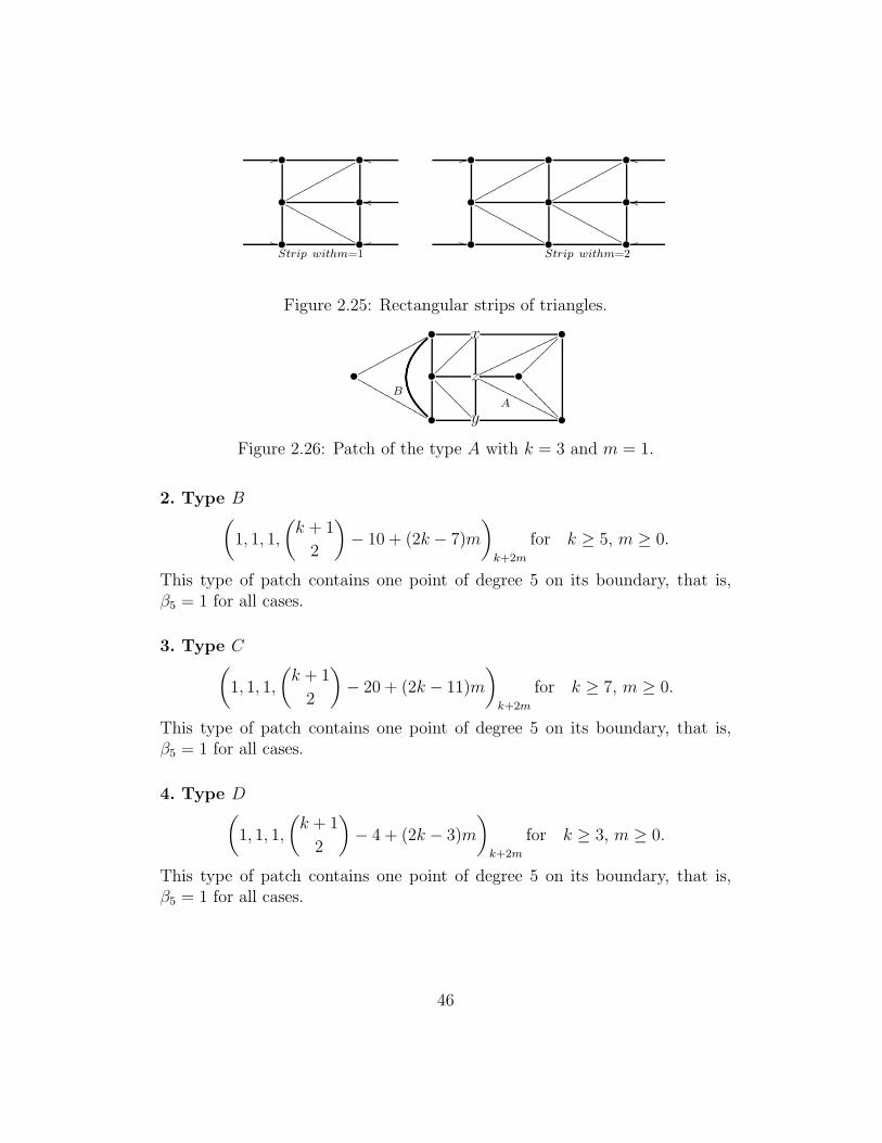
/• •
ppppppppppp o
•
NNNNNNNNNNN • oo
/•Strip withm=1
• o
/• •
ppppppppppp •
ppppppppppp o
•
NNNNNNNNNNN •
NNNNNNNNNNN •oo
/• •Strip withm=2
•o
Figure 2.25: Rectangular strips of triangles.
• x
~~~~
~~~ •
•
ppppppppppp
B
MMMMMMMMMMMM •
????
??? z
AOOOOOOOOOOOOO
ooooooooooooo •
????
????
~~~~~~~
• y •
Figure 2.26: Patch of the type A with k = 3 and m = 1.
2. Type B(
1, 1, 1,
(
k + 1
2
)
− 10 + (2k − 7)m
)
k+2m
for k ≥ 5, m ≥ 0.
This type of patch contains one point of degree 5 on its boundary, that is,β5 = 1 for all cases.
3. Type C(
1, 1, 1,
(
k + 1
2
)
− 20 + (2k − 11)m
)
k+2m
for k ≥ 7, m ≥ 0.
This type of patch contains one point of degree 5 on its boundary, that is,β5 = 1 for all cases.
4. Type D(
1, 1, 1,
(
k + 1
2
)
− 4 + (2k − 3)m
)
k+2m
for k ≥ 3, m ≥ 0.
This type of patch contains one point of degree 5 on its boundary, that is,β5 = 1 for all cases.
46

5. Type E(
1, 1, 1,
(
k + 1
2
)
− 40 + (2k − 15)m
)
k+2m
for k ≥ 10, m ≥ 0.
This type of patch contains one point of degree 5 on its boundary, that is,β5 = 1 for all cases.
6. Type F(
1, 1, 1,
(
k + 1
2
)
− 124 + (2k − 27)m
)
k+2m
for k ≥ 18, m ≥ 0.
This type of patch contains one point of degree 5 on its boundary, that is,β5 = 1 for all cases.
7. Type G(
1, 1, 1,
(
k + 1
2
)
− 76 + (2k − 21)m
)
k+2m
for k ≥ 14, m ≥ 0.
This type of patch contains one point of degree 5 on its boundary, that is,β5 = 1 for all cases.
8. Type H(
1, 1, 1,
(
k + 1
2
)
− 4
)
k
for k ≥ 3.
This type of patch can be constructed by using the generic construction methodwith β5 = 1 for (k−3) times from the patch (1, 1, 1, 2)3. These patches containone point of degree 5 on their boundary, that is, β5 = 1 for all cases.
9. Type I(
1, 1, 1,
(
k + 1
2
)
− 8
)
k
for k ≥ 4.
This type of patch can be constructed by using the generic construction methodwith β5 = 1 for (k−4) times from the patch (1, 1, 1, 2)4. These patches containone point of degree 5 on their boundary, that is, β5 = 1 for all cases.
47

10. Type J(
1, 1, 1,
(
k + 1
2
)
− 10
)
k
for k ≥ 5.
This type of patch can be constructed by using the generic construction methodwith β5 = 1 for (k−5) times from the patch (1, 1, 1, 5)5. These patches containone point of degree 5 on their boundary, that is, β5 = 1 for all cases.
11. Type K(
1, 1, 1,
(
k + 1
2
)
− 16
)
k
for k ≥ 6.
This type of patch can be constructed by using the generic construction methodwith β5 = 1 for (k−6) times from the patch (1, 1, 1, 5)6. These patches containone point of degree 5 on their boundary, that is, β5 = 1 for all cases.
12. Type L(
1, 1, 1,
(
k + 1
2
)
− 20
)
k
for k ≥ 7.
This type of patch can be constructed by using the generic construction methodwith β5 = 1 for (k−7) times from the patch (1, 1, 1, 8)7. These patches containone point of degree 5 on their boundary, that is, β5 = 1 for all cases.
13. Type M(
1, 1, 1,
(
k + 1
2
)
− 26
)
k
for k ≥ 8.
This type of patch can be constructed by using the generic construction methodwith β5 = 1 for (k−8) times from the patch (1, 1, 1, 10)8. These patches containone point of degree 5 on their boundary, that is, β5 = 1 for all cases.
14. Type N(
1, 1, 1,
(
k + 1
2
)
− 34
)
k
for k ≥ 9.
This type of patch can be constructed by using the generic construction methodwith β5 = 1 for (k−9) times from the patch (1, 1, 1, 11)9. These patches containone point of degree 5 on their boundary, that is, β5 = 1 for all cases.
48

15. Type O(
1, 1, 1,
(
k + 1
2
)
− 40
)
k
for k ≥ 10.
This type of patch can be constructed by using the generic construction methodwith β5 = 1 for (k − 10) times from the patch (1, 1, 1, 15)10. These patchescontain one point of degree 5 on their boundary, that is, β5 = 1 for all cases.
16. Type P(
1, 1, 1,
(
k + 1
2
)
− 44
)
k
for k ≥ 10.
This type of patch can be constructed by using the generic construction methodwith β5 = 1 for (k − 10) times from the patch (1, 1, 1, 11)10. These patchescontain one point of degree 5 on their boundary, that is, β5 = 1 for all cases.
2.7 Some Known Patches
2.7.1 Triangular Boundary
(a3, a4, a5, a6)3 patch P boundary remark
(0, 3, 0, 0)3 {123} 123 f3 = 1, β4 = 3(1, 0, 3, 0)3 {124, 134, 234} 123 f3 = 3, β5 = 3(1, 1, 1, 2)3 {125, 145, 245, 134, 234} 123 f3 = 5, β5 = 1
Table 2.1: Some patches with boundary length 3
49

2.7.2 Rectangular Boundary
(a3, a4, a5, a6)4 patch P boundary remark
(0, 1, 4, 0)4 {125, 145, 235, 345} 1234 f3 = 4β5 = 4
(0, 2, 2, 0)4 {123, 124} 1324 f3 = 2β4 = 2β5 = 2
(0, 2, 2, 2)4 {136, 145, 156, 236, 245, 256} 1423 f3 = 6β5 = 2
(0, 2, 2, 3)4 {127, 145, 157, 236, 267, 345, 356, 567} 1234 f3 = 8β5 = 1
(1, 0, 3, 2)4 {126, 135, 156, 245, 256, 345} 1243 f3 = 6β5 = 2
(1, 0, 3, 4)4 {123, 124, 134, 238, 247, 278 5678 f3 = 10346, 356, 358, 467} β5 = 1
(1, 1, 1, 2)4 {123, 124, 134, 235} 2435 f3 = 4β4 = 1β5 = 1
Table 2.2: Some patches with boundary length 4
50
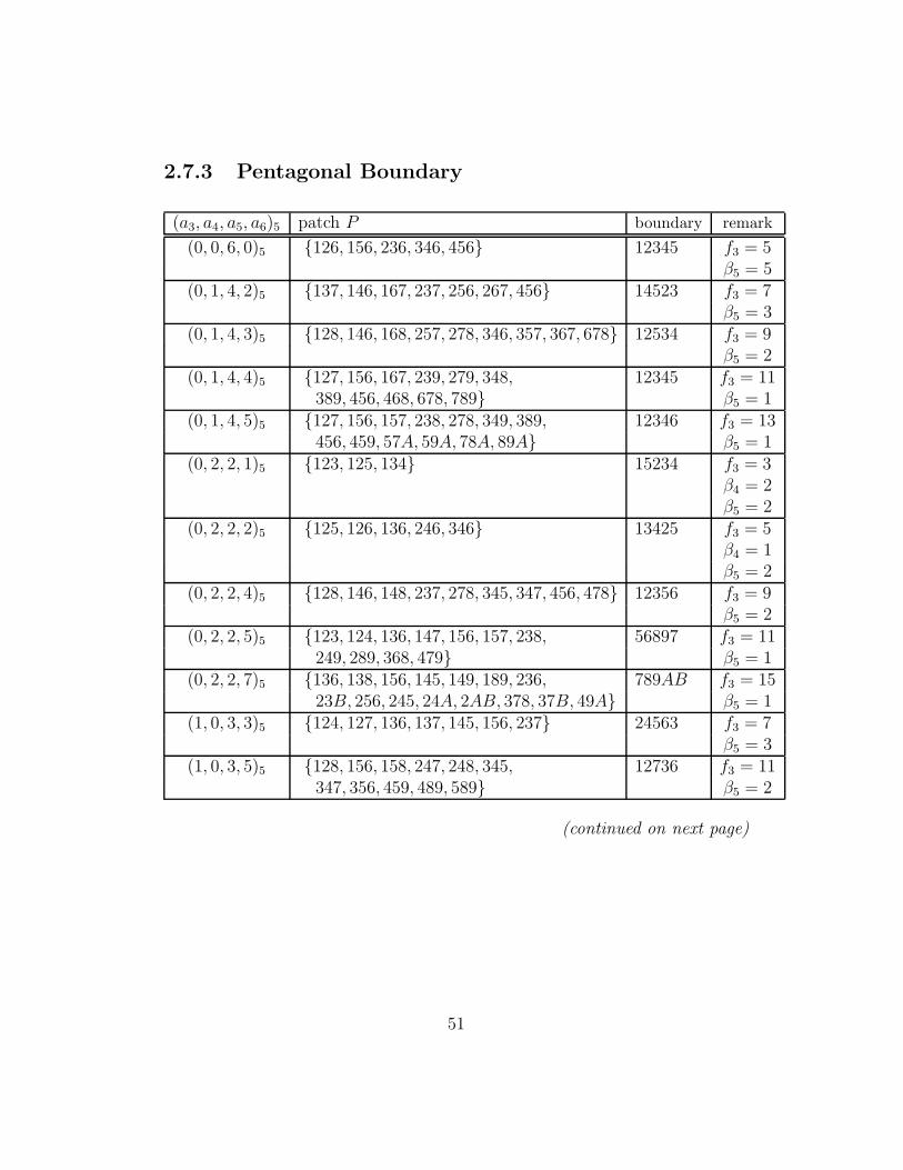
2.7.3 Pentagonal Boundary
(a3, a4, a5, a6)5 patch P boundary remark
(0, 0, 6, 0)5 {126, 156, 236, 346, 456} 12345 f3 = 5β5 = 5
(0, 1, 4, 2)5 {137, 146, 167, 237, 256, 267, 456} 14523 f3 = 7β5 = 3
(0, 1, 4, 3)5 {128, 146, 168, 257, 278, 346, 357, 367, 678} 12534 f3 = 9β5 = 2
(0, 1, 4, 4)5 {127, 156, 167, 239, 279, 348, 12345 f3 = 11389, 456, 468, 678, 789} β5 = 1
(0, 1, 4, 5)5 {127, 156, 157, 238, 278, 349, 389, 12346 f3 = 13456, 459, 57A, 59A, 78A, 89A} β5 = 1
(0, 2, 2, 1)5 {123, 125, 134} 15234 f3 = 3β4 = 2β5 = 2
(0, 2, 2, 2)5 {125, 126, 136, 246, 346} 13425 f3 = 5β4 = 1β5 = 2
(0, 2, 2, 4)5 {128, 146, 148, 237, 278, 345, 347, 456, 478} 12356 f3 = 9β5 = 2
(0, 2, 2, 5)5 {123, 124, 136, 147, 156, 157, 238, 56897 f3 = 11249, 289, 368, 479} β5 = 1
(0, 2, 2, 7)5 {136, 138, 156, 145, 149, 189, 236, 789AB f3 = 1523B, 256, 245, 24A, 2AB, 378, 37B, 49A} β5 = 1
(1, 0, 3, 3)5 {124, 127, 136, 137, 145, 156, 237} 24563 f3 = 7β5 = 3
(1, 0, 3, 5)5 {128, 156, 158, 247, 248, 345, 12736 f3 = 11347, 356, 459, 489, 589} β5 = 2
(continued on next page)
51

(continued from previous page)
(a3, a4, a5, a6)5 patch P boundary remark
(1, 0, 3, 6)5 {125, 159, 179, 238, 258, 346, 368, 12347 f3 = 13469, 479, 569, 56A, 58A, 68A} β5 = 1
(1, 0, 3, 7)5 {12A, 158, 15A, 237, 27A, 346, 367, 456, 12348 f3 = 15458, 569, 59A, 67B, 69B, 79A, 79B} β5 = 1
(1, 1, 1, 4)5 {127, 145, 157, 235, 257, 345, 346} 12364 f3 = 7β4 = 1
(1, 1, 1, 5)5 {125, 157, 167, 238, 258, 345, 358, 457, 467} 12346 f3 = 9β5 = 1
(1, 1, 1, 7)5 {126, 156, 158, 239, 269, 347, 379, 12348 f3 = 13457, 458, 56A, 57A, 679, 67A} β5 = 1
(1, 1, 1, 11)5 {125, 128, 134, 137, 145, 178, 245, ABCDE f3 = 21234, 239, 289, 376, 369, 67B, 69E, 6AB, β5 = 16AE, 78C, 7BC, 8CD, 89D, 9DE}
Table 2.3: Some patches with boundary length 5
52

2.7.4 Hexagonal Boundary
(a3, a4, a5, a6)6 patchP boundary remark
(0, 0, 6, 1)6 {123, 127, 134, 145, 156, 167} 234567 f3 = 6β5 = 6
(0, 0, 6, 2)6 {134, 135, 148, 234, 236, 247, 356, 478} 156278 f3 = 8β5 = 4
(0, 0, 6, 3)6 {146, 147, 169, 245, 247, 258, 356, 358, 172839 f3 = 10369, 456} β5 = 3
(0, 0, 6, 4)6 {129, 12A, 136, 139, 16A, 245, 249, 25A, 374586 f3 = 12379, 479, 58A, 68A} β5 = 2
(0, 0, 6, 6)6 {12A, 167, 16A, 23B, 2AB, 34C, 3BC, 458, 123457 f3 = 1648C, 567, 568, 689, 69A, 89C, 9AB, 9BC} β5 = 1
(0, 1, 4, 2)6 {126, 127, 136, 256, 346, 456} 134527 f3 = 6β4 = 1β5 = 3
(0, 1, 4, 3)6 {136, 138, 178, 234, 238, 278, 345, 356} 172456 f3 = 8β5 = 4
(0, 1, 4, 5)6 {128, 157, 158, 23A, 28A, 349, 39A, 456, 123467 f3 = 12459, 567, 589, 89A} β5 = 2
(0, 1, 4, 6)6 {129, 167, 169, 258, 259, 34A, 358, 35A, 128347 f3 = 14467, 46A, 59B, 5AB, 69B, 6AB} β5 = 2
(0, 2, 2, 2)6 {123, 124, 235, 146} 135246 f3 = 4β4 = 2β5 = 2
(0, 2, 2, 4)6 {126, 146, 147, 258, 268, 346, 358, 368} 125347 f3 = 8β4 = 1β5 = 1
(0, 2, 2, 5)6 {125, 159, 179, 258, 268, 345, 358, 368, 126347 f3 = 10459, 479} β5 = 2
(0, 3, 0, 3)6 {123, 125, 134, 236} 152634 f3 = 4β4 = 3
(0, 3, 0, 4)6 {125, 127, 147, 237, 346, 347} 152364 f3 = 6β4 = 2
(continued on next page)
53

(continued from previous page)
(a3, a4, a5, a6)6 patchP boundary remark
(0, 3, 0, 6)6 {126, 156, 157, 238, 268, 349, 389, 469, 123457 f3 = 10456, 689} β4 = 1
(1, 0, 3, 5)6 {129, 145, 159, 235, 259, 358, 368, 458, 123674 f3 = 10478, 678} β5 = 2
(1, 0, 3, 6)6 {145, 147, 158, 256, 258, 269, 346, 347, 182937 f3 = 12369, 45A, 46A, 56A} β5 = 3
(1, 0, 3, 7)6 {126, 156, 159, 26A, 28A, 347, 37A, 38A, 128349 f3 = 14457, 459, 56B, 57B, 67A, 67B} β5 = 2
(1, 0, 3, 8)6 {126, 156, 159, 237, 267, 378, 38A, 78B 123A49 f3 = 16458, 459, 48A, 56B, 58B, 67C, 6BC, 7BC} β5 = 2
(1, 0, 3, 9)6 {126, 15B, 16B, 237, 267, 34C, 37C, 49A, 1234A5 f3 = 1849C, 59A, 59B, 678, 68B, 7CD, 8CD, β5 = 178D, 89B, 89C}
(1, 1, 1, 5)6 {128, 145, 158, 256, 258, 345, 347, 356} 126374 f3 = 8β4 = 1β5 = 1
(1, 1, 1, 13)6 {123, 124, 134, 245, 258, 28G, 23G, 346, 7BEDAF f3 = 24369, 39G, 45C, 46C, 5BC, 57B, 578, β5 = 16CD, 69A, 6AD, 78F, 89G, 89F, 9AF,BCE,CDE}
Table 2.4: Some patches with boundary length 6
54
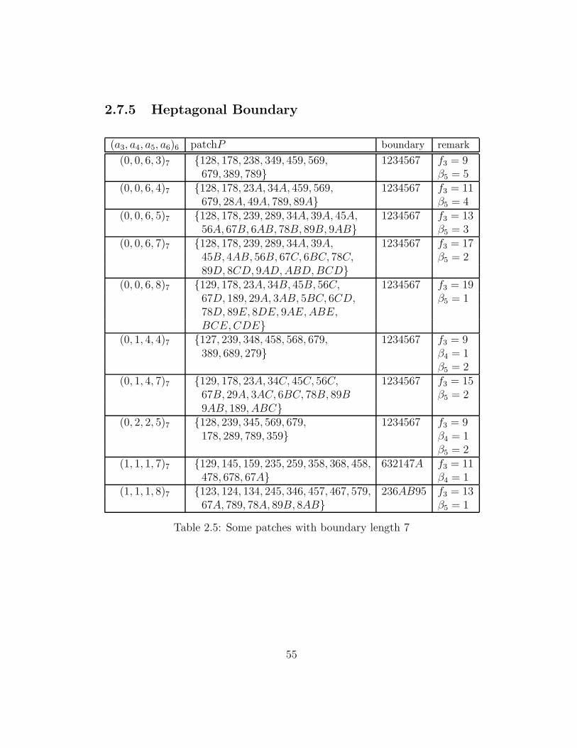
2.7.5 Heptagonal Boundary
(a3, a4, a5, a6)6 patchP boundary remark
(0, 0, 6, 3)7 {128, 178, 238, 349, 459, 569, 1234567 f3 = 9679, 389, 789} β5 = 5
(0, 0, 6, 4)7 {128, 178, 23A, 34A, 459, 569, 1234567 f3 = 11679, 28A, 49A, 789, 89A} β5 = 4
(0, 0, 6, 5)7 {128, 178, 239, 289, 34A, 39A, 45A, 1234567 f3 = 1356A, 67B, 6AB, 78B, 89B, 9AB} β5 = 3
(0, 0, 6, 7)7 {128, 178, 239, 289, 34A, 39A, 1234567 f3 = 1745B, 4AB, 56B, 67C, 6BC, 78C, β5 = 289D, 8CD, 9AD,ABD,BCD}
(0, 0, 6, 8)7 {129, 178, 23A, 34B, 45B, 56C, 1234567 f3 = 1967D, 189, 29A, 3AB, 5BC, 6CD, β5 = 178D, 89E, 8DE, 9AE,ABE,BCE,CDE}
(0, 1, 4, 4)7 {127, 239, 348, 458, 568, 679, 1234567 f3 = 9389, 689, 279} β4 = 1
β5 = 2(0, 1, 4, 7)7 {129, 178, 23A, 34C, 45C, 56C, 1234567 f3 = 15
67B, 29A, 3AC, 6BC, 78B, 89B β5 = 29AB, 189, ABC}
(0, 2, 2, 5)7 {128, 239, 345, 569, 679, 1234567 f3 = 9178, 289, 789, 359} β4 = 1
β5 = 2(1, 1, 1, 7)7 {129, 145, 159, 235, 259, 358, 368, 458, 632147A f3 = 11
478, 678, 67A} β4 = 1(1, 1, 1, 8)7 {123, 124, 134, 245, 346, 457, 467, 579, 236AB95 f3 = 13
67A, 789, 78A, 89B, 8AB} β5 = 1
Table 2.5: Some patches with boundary length 7
55

2.7.6 Some Other Used Patches
(a3, a4, a5, a6)6 patchP boundary remark
(0, 0, 6, 5)8 {123, 12A, 134, 14B, 1AB, 235, 367, 258964BA f3 = 12357, 346, 578, 679, 789} β5 = 4
(0, 0, 6, 12)8 {123, 125, 134, 146, 15I, 16I, 259, 46A, 234AGHF9 f3 = 2659C, 57C, 57I, 68D, 68I, 6AD, 78B, β5 = 278I, 7BC, 8BD, 9CF,ADG,BCE,BDE,CEF,DEG,EFH,EGH}
(1, 0, 3, 15)8 {126, 12E, 156, 159, 19D, 1DE, 26A, CDEFGHIJ f3 = 282A8, 28F, 2EF, 347, 37A, 3A8, 38H, β5 = 23HI, 34I, 457, 459, 49J, 4JI, 56B,57B, 67A, 67B, 8GH, 8GF, 9CD,9CJ}
(1, 1, 1, 10)8 {123, 124, 134, 23A, 25A, 257, 247, 5BDC6897 f3 = 1636A, 368, 348, 479, 489, 5AB, 6AC, β4 = 1ABC,BCD} β5 = 1
(1, 1, 1, 11)9 {123, 124, 236, 246, 356, 467, 569, 589, 1358CEA74 f3 = 17679, 79A, 89B, 9AB, 8BC,ABE, β5 = 1BCD,BDE,CDE}
(1, 1, 1, 11)10 {123, 124, 136, 234, 345, 358, 368, 1457DECB96 f3 = 16578, 689, 78A, 7AD, 89A, 9AB, β4 = 1ABC,ACD,CDE} β5 = 1
(1, 1, 1, 15)10 {123, 129, 19B, 234, 24A, 28A, 289, 1367FGHIEB f3 = 24346, 456, 45D, 4AD, 567, 57G, β4 = 15GH, 5DH, 7FG, 89A, 9AC, 9BC, β5 = 1ACD,BCE,CDI, CEI,DHI}
(1, 1, 1, 14)12 {123, 124, 136, 234, 345, 358, 368, 587, 1457BGHFED96 f3 = 20689, 78A, 7AB, 89A, 9AD,ADC, β4 = 1ABC,CDE,CEF,CFG,BCG, FGH} β5 = 1
Table 2.6: Some other known used patches
56

Chapter 3
Elliptic Triangulations ofSpheres
Let T be a triangulation of a sphere. For a point x ∈ T , the number of trianglesσ1, σ2, . . . , σd which contain x is denoted by d = d(x) and is called the degreeof x ∈ T. We can easily see that d ≥ 3. For a given triangulation T of a sphere,let us denote the face numbers of T by fi = fi(T ) (i = 1, 2, 3). That is, f1 isthe number of points, f2 the number of edges and f3 the number of trianglesin T. Then we have the following relation between the face numbers:
2f2(T ) = 3f3(T ). (3.1)
The integer χ(T ) = f1(T )−f2(T )+f3(T ) is called Euler’s characteristic. Nowfor d ≥ 3, define the nonnegative integer αd as the number of points in Twhich have degree equal to d, that is,
αd(T ) = αd = |{x ∈ T : d(x) = d }| . (3.2)
The tuple of numbers(α3, α4, α5, . . . , αm)
is called the parameters or the system of parameters of the triangulation. Fromthe definition of αd we obtain the equations
α3 + α4 + α5 + α6 + α7 + α8 + ...+ αm = f1(T ); (3.3)
3α3 + 4α4 + 5α5 + 6α6 + 7α7 + 8α8 + ... +mαm = 2f2(T ); (3.4)
3α3 + 4α4 + 5α5 + 6α6 + 7α7 + 8α8 + ... +mαm = 3f3(T ). (3.5)
By taking the combination 6(3.3)− 3(3.4) + 2(3.5) we easily get
3α3 + 2α4 + α5 − α7 − 2α8 − . . .− (m− 6)αm = 6χ(T ). (3.6)
57

In the case of spherical triangulations we get χ(T ) = 2 and equation (3.6)becomes
3α3 + 2α4 + α5 − α7 − 2α8 − . . .− (m− 6)αm = 12. (3.7)
A triangulation T is called elliptic if it does not contain any point withdegree greater than 6, that is, d(x) ≤ 6 for every x ∈ T. If T is an elliptictriangulation, equation (3.7) becomes
3α3 + 2α4 + α5 = 12. (3.8)
There are exactly 19 solutions (α3, α4, α5) for (3.8). These are
(0, 0, 12); (0, 1, 10); (0, 2, 8); (0, 3, 6); (0, 4, 4); (0, 5, 2); (0, 6, 0);
(1, 0, 9); (1, 1, 7); (1, 2, 5); (1, 3, 3); (1, 4, 1); (2, 0, 6);
(2, 1, 4); (2, 2, 2); (2, 3, 0); (3, 0, 3); (3, 1, 1); (4, 0, 0).
For any system of nonnegative integers (a3, a4, a5) which satisfies the equation3a3 + 2a4 + a5 = 12, it is known by an old result of Eberhard (1910) [3] thatthere exist nonnegative integer values N = a6 ≥ 0 and a triangulation T withthe property:
(α3(T ), α4(T ), α5(T ), α6(T )) = (a3, a4, a5, a6).
Let S be the following set of integral 4-tuples:
S = {(3, 1, 1, 2m)|m ≥ 0} ∪ {(4, 0, 0, 2m+ 1)|m ≥ 0}
∪ {(0, 0, 12, 1), (0, 1, 10, 0), (0, 1, 10, 1), (0, 4, 4, 1), (0, 5, 2, 1),
(0, 6, 0, 1), (1, 0, 9, 0), (1, 0, 9, 1), (1, 0, 9, 2), (1, 0, 9, 4), (1, 1, 7, 0),
(1, 1, 7, 1), (1, 2, 5, 0), (1, 4, 1, 0), (1, 4, 1, 1), (2, 0, 6, 1), (2, 1, 4, 0),
(2, 3, 0, 1), (2, 3, 0, 3), (2, 3, 0, 7), (2, 3, 0, 15), (2, 3, 0, 31), (3, 0, 3, 0),
(3, 0, 3, 2), (3, 0, 3, 4), (3, 0, 3, 12), (3, 1, 1, 1),
(3, 1, 1, 17), (4, 0, 0, 2). }
We shall show that if (a3, a4, a5, a6) is not contained in the set S, then thereexists an (elliptic) triangulation T of the sphere with the system of parameters
(α3(T ), α4(T ), α5(T ), α6(T )) = (a3, a4, a5, a6).
We remark that the nonexistence of triangulations (3, 1, 1, 2m) and (4, 0, 0,2m + 1) for m ≥ 0 have been shown by Grunbaum and Motzkin in [5] (seealso [4]).
We shall use the following constructive methods to find the elliptic sphericaltriangulations:
58

1. Mutant, productive and self-reproductive configurations.
2. Fullering constructions.
3. Glueing of Patches.
3.1 Mutant Configurations
A configuration is called mutant if adding (deleting) one or more points to(of) it changes the parameters of its triangulation in a certain way. We shalldescribe two types of mutant configurations where one point is added.
3.1.1 Type M1 :
Let X = {x, y, z} with a triangle xyz and assume that d(x) = d(y) =d(z) = 5. Then the insertion of a new point P and the replacement of xyzby pxy, pxz, pyz leads to a new triangulation T ′ with d′(x) = d′(y) = d′(z) =6, d′(P ) = 3 (refer to Figure 3.1). Hence
(α3(T′), α4(T
′), α5(T′), α6(T
′)) = (α3(T ) + 1, α4(T ), α5(T )− 3, α6(T ) + 3).
We say that X is a mutant configuration of type M1.
x(5)
����
����
����
�
7777
7777
7777
7
y(5)T
z(5)
−→
x(6)
4444
4444
4444
444
P (3)
xxxxxxxx
FFFFFFFF
y(6)T′
z(6)
Figure 3.1: Mutant configuration of type M1.
3.1.2 Type M2 :
Let X = {x, y, z} with a triangle xyz and assume that d(x) = d(z) =5, d(y) = 4. Then the insertion of a new point P and the replacement of
59

xyz by pxy, pxz, pyz leads to a new triangulation T ′ with d′(x) = d′(z) =6, d′(P ) = 3, d′(y) = 5 (refer to Figure 3.2). Hence
(α3(T′), α4(T
′), α5(T′), α6(T
′)) = (α3(T ) + 1, α4(T )− 1, α5(T )− 1, α6(T ) + 2).
We say that X is a mutant configuration of type M2.
x(5)
����
����
����
�
7777
7777
7777
7
y(4)T
z(5)
−→
x(6)
4444
4444
4444
444
P (3)
xxxxxxxx
FFFFFFFF
y(5)T′
z(6)
Figure 3.2: Mutant configuration of type M2.
3.2 Productive and Self-Reproductive Config-
urations
Let T be any triangulation with point set V. A subset of points X ⊂ V iscalled a productive configuration if it satisfies the following property:At least one point (say z) can be added to X and certain changes involvingtriangles of X∪{z} can be made to the triangulation T such that the number ofpoints of degree six is increased whereas the number of points of degrees 3,4,5remain unchanged.
A subset of points X ⊂ V is called a self-reproductive configuration if itsatisfies the following property:At least one point (say z) can be added to X and certain changes involvingtriangles of X ∪ {z} can be made to the triangulation T such that
(i) the number of points of degree six is increased whereas the number of pointsof degrees less than six remain unchanged;
(ii) the resulting new triangulation contains the original configuration as asubconfiguration.
60

3.2.1 Type P1 :
Let X = {p, x, q, y} with two triangles pxy, qxy and assume that d(p) = 4,d(q) = 5, d(x) = d(y) = 6. Then the insertion of a new point z and thereplacement of pxy, qxy by pxz, pyz, qxz, qyz leads to a new triangulation T ′
with d′(x) = d′(y) = d′(q) = 6, d′(p) = 5, d′(z) = 4 (refer to Figure 3.3).Hence
(α3(T′), α4(T
′), α5(T′), α6(T
′)) = (α3(T ), α4(T ), α5(T ), α6(T ) + 1).
We say that X is a productive configuration of type P1.
x(6)
�����
p(4)
????
?
q(5)
?????
y(6)
T����
�−→ x(6)
�����
p(5)
????
?
q(6)
?????
y(6)
T′����
�
Figure 3.3: Mutant configuration of type P1.
3.2.2 Type P2 :
v
����
����
@@@@
@@@ w
@@@@
@@@@
}}}}
}}}}
u
>>>>
>>>> P
����
����
@@@@
@@@@ x
����
����
zT
y
−→
v
����
����
@@@@
@@@ w
@@@@
@@@@
}}}}
}}}}
u
>>>>
>>>> P
����
����
@@@@
@@@@ x
����
����
zT′
y
qiiiiiiiiiiiiiiiiiii
Figure 3.4: Productive configuration of type P2.
Let X = {u, v, w, p, x, y, z} with six triangles upv, vpw, wpx, xpy, ypz, upzand assume that d(p) = d(v) = 6, d(u) = d(y) = 5 and d(w) = d(x) = d(z) =4. Then the insertion of a new point q and the replacement of upv, vpw byupq, uqv, pqw, qvw leads to a new triangulation T ′ with d′(u) = 6, d′(w) =5, d′(q) = 4 (refer to Figure 3.4). Hence
(α3(T′), α4(T
′), α5(T′), α6(T
′)) = (α3(T ), α4(T ), α5(T ), α6(T ) + 1).
61

We say that X is a productive configuration of type P2.Clearly, every self-reproductive configuration must contain at least one pro-
ductive configuration. We give a list of self-reproductive configurations withpoints of degree six or less each. These are of fundamental importance in theconstructions which follow.
3.2.3 Type A :
Let xyz be any triple of points in the triangulation T and assume that X ={x, y, z} forms a triangle in T with the degrees given as d(x) = 3, d(y) = 4,d(z) = 5. If we delete the triangle xyz from T, and add a point p and threenew triangles pxy, pxz, pyz then we get a new triangulation T ′ with the degreesd′(p) = 3, d′(x) = 4, d′(y) = 5, d′(z) = 6. The degrees of all the other points ofT remain the same. Hence T ′ = T ∪ {p} has the parameters
(α3(T′), α4(T
′), α5(T′), α6(T
′)) = (α3(T ), α4(T ), α5(T ), α6(T ) + 1).
We thus see that X is a productive configuration as well as self-reproductiveconfiguration, since in T ′ the configuration pxy is isomorphic to X (refer toFigure 3.5). Such a configuration X will be called a self-reproductive configu-ration of type A.
x(3)
����
����
����
�
7777
7777
7777
7
y(4)T
z(5)
−→
x(4)
4444
4444
4444
444
P (3)
xxxxxxxx
FFFFFFFF
y(5)T′
z(6)
Figure 3.5: Self-reproductive configuration of type A.
3.2.4 Type B1:
Let vwxyz be any five points of the triangulation T and assume that X ={v, w, x, y, z} contains exactly four triangles vxy, vxz, wxy, wxz of T such thatthe degrees of the points are given as d(v) = d(w) = d(x) = 4, d(y) = d(z) = 6.If we delete these given four triangles from T and add two new points p, q and
62

eight new triangles vpx, vpy, vqx, vqz, wpx, wpy, wqx, wqz then we get a newtriangulation T ′ with the degrees d′(p) = d′(q) = 4, d′(v) = d′(w) = 6. Thedegrees of the other points of T remain the same. Hence the triangulationT ′ = T ∪ {p, q} will have the parameters
(α3(T′), α4(T
′), α5(T′), α6(T
′)) = (α3(T ), α4(T ), α5(T ), α6(T ) + 2).
Thus X is a productive as well as self-reproductive configuration, since inT ′ the configuration pqvwx is isomorphic to X (refer to Figure 3.6). Such aconfiguration X will be called a self-reproductive configuration of type B1.
y
����
����
����
�
9999
9999
9999
9
v(4)
9999
9999
9999
9 x(4) w(4)
T
����
����
����
�
z
−→
y
6666
6666
6666
66
p
wwww
wwww
w
HHHHHHHHH
v(6)
GGGGGG
GGG
6666
6666
6666
66x(4) w(6)
vvvvvvvvv
T′
����
����
����
��
q
z
Figure 3.6: Self-reproductive configuration of type B1.
3.2.5 Type B2:
Let vwxy be any four points of the triangulation T and assume that X ={v, w, x, y} contains exactly two triangles vwx, vwy of T such that the degreesof the points are given as d(v) = d(w) = 4, d(x) = d(y) = 5. If we deletethese two triangles from T and add two new points p, q and six new trian-gles vqx, vpq, vpy, wqx, wpq, wpy then we get a new triangulation T ′ with thedegrees d′(p) = d′(q) = 4, d′(v) = d′(w) = 5, d′(x) = d′(y) = 6. Hence thetriangulation T ′ = T ∪ {p, q} will have the parameters
(α3(T′), α4(T
′), α5(T′), α6(T
′)) = (α3(T ), α4(T ), α5(T ), α6(T ) + 2).
Thus X is a productive as well as self-reproductive configuration, since inT ′ the configuration pwqv is isomorphic to X (refer to Figure 3.7). Such aconfiguration X will be called a self-reproductive configuration of type B2.
63

x(5)
����
����
����
�
8888
8888
8888
8
v(4)
7777
7777
7777
7 w(4)
T
����
����
����
�
y(5)
−→
x(6)
5555
5555
5555
55
q
wwwww
wwww
HHHHHHHHH
v(5)
7777
7777
7777
7 p w(5)
T′
����
����
����
�
y(6)
Figure 3.7: Self-reproductive configuration of type B2.
3.2.6 Type C :
Let vwxyz be any five points of the triangulation T and assume that X ={v, w, x, y, z} contains three triangles vwx, wxy, xyz of T such that the degreesof the points are given as d(w) = 4 and d(v) = d(x) = d(y) = d(z) = 5.
x(5)
||||
||||
||
CCCC
CCCC
CCz(5)
v(5)
CCCC
CCCC
CCy(5)
T
||||
||||
||
w(4)
−→
x(5)
����
����
���
BBBB
B z(6)
~~~~
~
p@@
@@@
�������������
v(5)
CCCC
CCCC
CCy(5)
T′
xxxxxxxxxx
w(5)
Figure 3.8: Self-reproductive configuration of type C.
If we delete the two triangles wxy, xyz from T, and add a point p with fournew triangles wpx, wpy, pxz, pyz then we get a new triangulation T ′ with thedegrees of points as d′(p) = 4, d′(w) = 5, d′(z) = 6 and the degrees of the otherpoints remain unchanged. Hence the new triangulation T ′ = T ∪ {p} has theparameters
(α3(T′), α4(T
′), α5(T′), α6(T
′)) = (α3(T ), α4(T ), α5(T ), α6(T ) + 1).
Thus X is a productive as well as self-reproductive configuration, since in T ′
the configuration pywvx is isomorphic to the configuration X (refer to Figure
64

??). Such a configuration X will be called a self-reproductive configurationof type C. Note that each such configuration of type C contains a pentagonaltriangle and a triangle of degrees 4, 5, 5.
3.2.7 Type D :
Let puvwxyz be any seven points in the triangulation T and assume that X ={p, u, v, w, x, y, z} has six triangles puv, pvw, pwx, pxy, pyz, pzu with degrees ofthe points given as d(p) = 6, d(w) = d(x) = d(y) = d(z) = 5, d(u) = 4, d(v) =6. If we delete the two triangles puv, pvw from T, and add one point q andfour new triangles pqu, pqw, quv, qvw, then we get a new triangulation T ′ withthe degrees of points as d′(q) = 4, d′(u) = 5, d′(w) = 6 and the degrees of theother points remain unchanged. Hence T ′ = T ∪ {p} has the parameters
(α3(T′), α4(T
′), α5(T′), α6(T
′)) = (α3(T ), α4(T ), α5(T ), α6(T ) + 1).
v(6)
4444
4444
4444
444
xxxx
xxxx
w(5)
FFFFFFFF
u(4)
FFFF
FFFF P (6)
x(5)
xxxxxxxx
z(5)T
y(5)
−→
v(6)
4444
4444
4444
444
xxxx
xxxx
w(6)
FFFFFFFF
q
lllllllllllllll
u(5)
FFFFF
FFF P (6)
x(5)
xxxxxxxx
z(5)T′
y(5)
Figure 3.9: Self-reproductive configuration of type D.
Thus X is a productive as well as self-reproductive configuration, since inT ′ the configuration pqwxyzu is isomorphic to the configuration X (refer toFigure 3.9). Such a configuration X will be called a self-reproductive configu-ration of type D.
3.2.8 Types E1 and E2 :
Let puvwxyz be any seven points in a triangulation T1 and assume that X ={p, u, v, w, x, y, z} contains six triangles puv, pvw, pwx, pxy, pyz, pzu with thedegrees of the points given as d(u) = d(x) = 4, d(v) = d(y) = 5, d(p) =d(w) = d(z) = 6. Also let another triangulation T2 be given with the set X
65

as above on seven points, where now the degrees are given as d(u) = d(w) =4, d(v) = d(z) = 6, d(x) = d(y) = 5, d(p) = 6.
v(5)
4444
4444
4444
444
xxxx
xxxx
w(6)
FFFFFFFF
u(4)
FFFF
FFFF P (6)
x(4)
xxxxxxxx
z(6)T1
y(5)
−→
v(6)
4444
4444
4444
444
xxxx
xxxx q
SSSSSSSSSSSSSSSS w(6)
FFFFFFFF
u(4)
FFFFF
FFF P (6)
x(5)
xxxxxxxx
z(6)T
′
1
y(5)
v(6)
4444
4444
4444
444
xxxx
xxxx
w(4)
FFFFFFFF
u(4)
FFFF
FFFF P (6)
x(5)
xxxxxxxx
z(6)T2
y(5)
−→
v(6)
4444
4444
4444
444
xxxx
xxxx
w(4)
FFFFFFFF
u(5)
FFFFF
FFF P (6)
qRRRRRRRRRRRRRRRR x(5)
xxxxxxxx
z(6)T′
2
y(6)
Figure 3.10: Self-reproductive configuration of types E1 and E2.
If we delete the two triangles pvw, pwx from T1, and add a point q and fournew triangles pqv, pqx, qvw, qxw then we get a new triangulation T ′
1 with thedegrees d′(q) = 4, d′(x) = 5, d′(v) = 6 and the degrees of the remaining pointsunchanged. Hence T ′
1 = T1 ∪ {q} has the parameters
(α3(T′1), α4(T
′1), α5(T
′1), α6(T
′1)) = (α3(T1), α4(T1), α5(T1), α6(T1) + 1).
Thus X is a self-reproductive configuration because the configuration pqvuzyxis isomorphic to the configuration X (in the triangulation T2) (refer to Figure3.10).
If we delete the two triangles pyz, pzu from T2, and add one point q and fournew triangles pqy, pqu, qyz, qzu then we get another new triangulation T ′
2 withthe degrees d′(q) = 4, d′(u) = 5, d′(y) = 6 and the degrees of the remainingpoints unchanged. Hence T ′
2 = T2 ∪ {q} has the parameters
(α3(T′2), α4(T
′2), α5(T
′2), α6(T
′2)) = (α3(T2), α4(T2), α5(T2), α6(T2) + 1).
66

Thus X is a self-reproductive configuration because the configuration pquvwxyis isomorphic to the configuration X in the triangulation T1 (refer to Figure3.10).
Hence from the given triangulation T1 we obtain a new triangulation T ′2
which has the parameters:
(α3(T′2), α4(T
′2), α5(T
′2), α6(T
′2)) = (α3(T1), α4(T1), α5(T1), α6(T1) + 2).
Since we can get the configuration X (in the triangulation T1) again after twosteps, X is called a self-reproductive configuration of types E1 and E2.
3.2.9 Type E3 :
Let puvwxyz be seven points in a triangulation T1 and assume that X ={p, u, v, w, x, y, z} contains six triangles puv, pvw, pwx, pxy, pyz, pzu with thedegrees of the points given as d(u) = d(x) = 4, d(v) = d(z) = 5, d(w) =d(y) = d(p) = 6.
Let a triangulation T2 be given with the set X as above on seven points,where now the degrees are given as d(u) = d(w) = 4, d(v) = d(y) = d(p) = 6,d(x) = d(z) = 5. Also let a triangulation T3 be given with the set X as aboveon seven points, where now the degrees are given as d(v) = 4, d(u) = d(x) =d(w) = d(z) = 5, d(p) = d(y) = 6.
If we delete the two triangles pvw, pwx from T1, and add a point q and fournew triangles pqv, pqx, qvw, qxw then we get a new triangulation T ′
1 with thedegrees d′(q) = 4, d′(x) = 5, d′(v) = 6 and the degrees of the remaining pointsunchanged. Hence T ′
1 = T1 ∪ {q} has the parameters
(α3(T′1), α4(T
′1), α5(T
′1), α6(T
′1)) = (α3(T1), α4(T1), α5(T1), α6(T1) + 1).
Thus X is a self-reproductive configuration because the set pqvuzyx is a con-figuration which is isomorphic to the configuration X in the triangulation T2
(refer to Figure 3.11).If we delete the two triangles pvw, puv from T2, and add one point q and
four new triangles puq, quv, pwq, qvw then we get a new triangulation T ′2 with
the degrees d′(q) = 4, d′(u) = 5, d′(w) = 5 and the degrees of the remainingpoints unchanged. Hence T ′
2 = T2 ∪ {q} has the parameters
(α3(T′2), α4(T
′2), α5(T
′2), α6(T
′2)) = (α3(T2), α4(T2)− 1, α5(T2) + 2, α6(T2)).
67
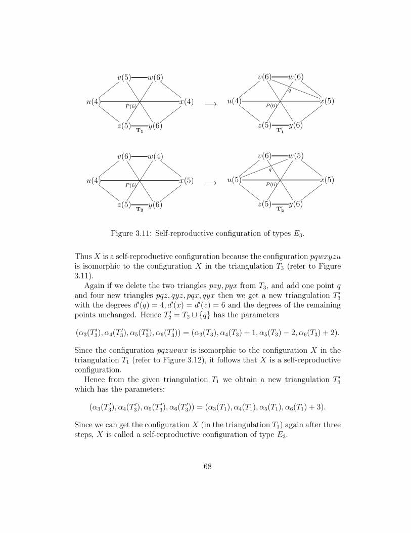
v(5)
4444
4444
4444
444
xxxx
xxxx
w(6)
FFFFFFFF
u(4)
FFFF
FFFF P (6)
x(4)
xxxxxxxx
z(5)T1
y(6)
−→
v(6)
4444
4444
4444
444
xxxx
xxxx
qSSSSSSSSSSSSSSSS w(6)
FFFFFFFF
u(4)
FFFFF
FFF P (6)
x(5)
xxxxxxxx
z(5)T
′
1
y(6)
v(6)
4444
4444
4444
444
xxxx
xxxx
w(4)
FFFFFFFF
u(4)
FFFF
FFFF P (6)
x(5)
xxxxxxxx
z(5)T2
y(6)
−→
v(6)
4444
4444
4444
444
xxxx
xxxx
w(5)
FFFFFFFF
q
lllllllllllllll
u(5)
FFFFF
FFF P (6)
x(5)
xxxxxxxx
z(5)T′
2
y(6)
Figure 3.11: Self-reproductive configuration of types E3.
Thus X is a self-reproductive configuration because the configuration pqwxyzuis isomorphic to the configuration X in the triangulation T3 (refer to Figure3.11).
Again if we delete the two triangles pzy, pyx from T3, and add one point qand four new triangles pqz, qyz, pqx, qyx then we get a new triangulation T ′
3
with the degrees d′(q) = 4, d′(x) = d′(z) = 6 and the degrees of the remainingpoints unchanged. Hence T ′
2 = T2 ∪ {q} has the parameters
(α3(T′3), α4(T
′3), α5(T
′3), α6(T
′3)) = (α3(T3), α4(T3) + 1, α5(T3)− 2, α6(T3) + 2).
Since the configuration pqzuvwx is isomorphic to the configuration X in thetriangulation T1 (refer to Figure 3.12), it follows that X is a self-reproductiveconfiguration.
Hence from the given triangulation T1 we obtain a new triangulation T ′3
which has the parameters:
(α3(T′3), α4(T
′3), α5(T
′3), α6(T
′3)) = (α3(T1), α4(T1), α5(T1), α6(T1) + 3).
Since we can get the configuration X (in the triangulation T1) again after threesteps, X is called a self-reproductive configuration of type E3.
68

v(4)
4444
4444
4444
444
xxxx
xxxx
w(5)
FFFFFFFF
u(5)
FFFF
FFFF P (6)
x(5)
xxxxxxxx
z(5)T3
y(6)
−→
v(4)
4444
4444
4444
444
xxxx
xxxx
w(5)
FFFFFFFF
u(5)
FFFFF
FFF P (6)
x(6)
xxxxxxxxq
kkkkkkkkkkkkkkkk
z(6)T
′
3
y(6)
Figure 3.12: Self-reproductive configuration of types E3.
3.2.10 Type G :
Let puvwxyz be any seven points in a triangulation T and assume that X ={p, u, v, w, x, y, z} contains six triangles puv, pvw, pwx, pxy, pyz, pzu with thedegrees of the points given as d(x) = d(v) = d(z) = d(p) = 6 and d(u) =d(w) = d(y) = 4.
v
0000
0000
0000
000
}}}}
}}}}
w(4)
BBBB
BBBB
B
���������������
u(4)
AAAA
AAAA P (6)
x
||||
||||
|
zT
y(4)
−→
v
;;;;
;;;;
;;;;
;;;;
;
}}}}
}}}}
w(6)
BBBB
BBBB
B
����
����
����
����
�q
jjjjjjjjjjjjjjjjj
su(6)
AAAA
AAAA P
r TTTTTTTTTTTTTTTTT x
||||
||||
|
zT′
y(6)
Figure 3.13: Self-reproductive configuration of types G.
If we delete the six triangles from T and add three new points q, r, s andtwelve new triangles upq, uqv, pqw, qvw, psw, psy, sxw, sxy, pur, pry, ruz, ryzthen we get a triangulation T ′ with the degrees d′(u) = d′(w) = d′(y) =6, d′(q) = d′(r) = d′(s) = 4 and the degrees of the remaining points unchanged.Hence T ′ = T ∪ {q, r, s} has the parameters
(α3(T′), α4(T
′), α5(T′), α6(T
′)) = (α3(T ), α4(T ), α5(T ), α6(T ) + 3).
Thus X is a productive and self-reproductive configuration, since in T ′ theconfiguration pqwsyru is isomorphic to the configuration X (refer to Figure3.13). Such a configuration X will be called a self-reproductive configurationof type G.
69

3.3 Fullering Constructions
Let T be a triangulation and let a, b be two integers such that 3 ≤ a < b andαd = 0 for d 6= a, b. The triangulation T is called a fullering triangulation if6 ∈ {a, b}.
Example: Note that
T = {156, 157, 167, 256, 258, 268, 357, 358, 378, 467, 468, 478}
is a triangulation with d(x) = 3 for x = 1, 2, 3, 4 and with d(x) = 6 forx = 5, 6, 7, 8. Hence T is a fullering triangulation.
3.3.1 Face-fullering of Triangulations
Let T be a triangulation with face numbers fk(T ) (k = 1, 2, 3). That is, f1(T )is the number of points, f2(T ) the number of edges and f3(T ) the number oftriangles in T. In this section we show that there exists a triangulation T1 withface numbers fk(T1) (k = 1, 2, 3) and parameters as follows:
f1(T1) = f1(T ) + f3(T ); f2(T1) = 3f2(T ); f3(T1) = 3f3(T ); (3.9)
αd(T1) = αd(T ) for d 6= 6 ; α6(T1) = α6(T ) + f3(T ). (3.10)
We also show that if T is a fullering (elliptic) triangulation, then T1 is also afullering (elliptic) triangulation.
For the construction of T1 we add one vertex point xσ for each triangleσ ∈ T to the vertex points of T : The set of vertices V1 of T1 is accordinglyV1 = V ∪ {xσ | σ is a triangle in T}. The new triangles for T1 will be all{x, xσ, xτ} where |σ ∩ τ | = 2 and x ∈ σ ∩ τ (see Figure 3.14).
We then obtain d1(x) = d(x) for points x ∈ T and d1(xσ) = 6 for thenew points xσ ∈ T1. Hence T1 possesses the property of being a fulleringtriangulation if T is a fullering triangulation and we also get (3.10). Thenumber of pairs {σ, τ} which are neighbours (that is, the pairs {σ, τ} with theproperty |σ ∩ τ | = 2) is the same as the integer f2(T ) (that is, the numberof edges of T ). Hence we obtain from (3.1) the equality f3(T1) = 2f2(T ) =3f3(T ), which verifies the third equation in (3.9). Applying (3.1) once morewe get
2f2(T1) = 3f3(T1) = 9f3(T ) = 6f2(T ).
70

⊡ ⊡
ooooooooo
•
MMMMMMMM
qqqqqqqq •??
????
⊡
MMMMMMMM ⊡
qqqqqqqq •
////
////
/
����
��
•
����
��•
OOOOOOOOO
qqqqqqqq
⊡ ⊡
Figure 3.14: Face-fullering of a triangulation
Cancelling the factor 2 from both ends of this equation, we arrive at the secondequation of (3.9). We may also verify the first equation of (3.9) by observingthat
2 = f1(T1)− f2(T1) + f3(T1) = f1(T1)− 3f2(T ) + 3f3(T )
= f1(T1)− 3f1(T ) + 6.
This gives us
f1(T1) = 3f1(T )− 4 = f1(T ) + 2f1(T )− 4 = f1(T ) + f3(T ).
This construction will be denoted by T1 = FF (T ) and will be called eitherthe face-fullering or the leapfrog of T.
3.3.2 Edge-fullering of Triangulations
In this section we construct a triangulation T2 with face numbers fk(T2) (k =1, 2, 3) and parameters as follows:
f1(T2) = f1(T ) + f2(T ); f2(T2) = 4f2(T ); f3(T2) = 4f3(T ); (3.11)
αd(T2) = αd(T ) for d 6= 6 ; α6(T2) = α6(T ) + f2(T ). (3.12)
As in the previous section it may be shown that if T2 is a fullering (elliptic)triangulation, then T2 is also a fullering (elliptic) triangulation.
For the construction of T2 we add a point xe for each edge e = xy of T. Hencethe point set V2 of T2 is just V2 = V ∪V E, where V E = {xe : e ∈ Edge(T )}.The new triangles of T2 are all {x, xe, xf} where e, f ⊂ σ and where x ∈ σ ∩ τfor some triangles σ, τ in T, together with triangles {xe, xf , xg} where {e, f, g}
71

are the edges of an old triangle (see Figure 3.15). Note that for the old verticesx ∈ V we get the same degree d2(x) = d(x), and for the new vertices xe weget the degree d2(xe) = 6. This construction will be denoted by T2 = EF (T )and will be called the edge-fullering of T.
⊡ •??
????
����
��
{{{{{{⊡
•
??????
????
?? •
����
��•
????
??
⊡ •??
????
����
��⊡ •
����
��
;;;;
;;
•
����
��•
????
?? •
����
��
⊡ •
{{{{
{{ ⊡
Figure 3.15: Edge-fullering of a triangulation
3.3.3 Edge-fullering of Patches
Let P be a patch with face numbers fk(P ) (k = 1, 2, 3). That is, f1(P )is the number of points, f2(P ) the number of edges and f3(P ) the number oftriangles in P . By using the same construction method as for the edge-fulleringof triangulations discussed in the previous section, it can be shown that thereexists a patch P2 with face numbers fk(P2) (k = 1, 2, 3) and parameters asfollows:
f1(P2) = f1(P )+f2(P ); f2(P2) = 2f2(P )+3f3(P ); f3(P2) = 4f3(P ); (3.13)
αd(P2) = αd(P ) for d 6= 6 ; α6(P2) = α6(P ) + f2(P ). (3.14)
Moreover, it can be shown that the boundary length b(P2) of P2 is twice thatof P, that is, b(P2) = 2b(P ).
This construction will be denoted by P2 = EF (P ) and will be called theedge-fullering of P.
72

3.4 Glueing of Patches
Let us consider two patches P : (α3, α4, α5, α6)b and P ′ : (α′3, α
′4, α
′5, α
′6)b′ . If
both patches have the same boundary length (that is, b = b′), then we canglue them to get a new patch (α3+α′
3, α4+α′4, α5+α′
5, (α6+α′6)+bm), where
m ≥ 0. The glueing can be done by using a circular strip of 2b triangles.We can also glue the patches by some special methods, which we describe
below:
3.4.1 Method A
Consider the patches of types (1, 1, 1,M)b and (1, 1, 1, N)b which contain apoint of degree five each on their boundary. If we glue these two patches bya belt, then we can get a triangulation of type (2, 2, 2,M + N + b). Thistriangulation can be arranged in such a way that the two points of degree 5are edge-related, that is, are connected by a sequence of edges (refer to Figure3.16(a)). Hence by inserting a new point of degree four between the twoexisting points of degree five, we obtain a triangulation of type (2, 3, 0,M +N + b+ 2).
•;;
;;;
����
� •;;
;;;
����
�P2 •
;;;;
;
����
�
•99
999 •
9999
9
����
� • •99
999
����
� •
����
�
•(a)
5P1
•
•
5555
5555
55 •99
999
P2
5
5555
5
����
�
•99
999
����
�
•
55555
(b)5
P1
•
•99
999
599
999
����
�P2 •
5555
5
����
�
•99
999 • •
����
�
5P1(c)
Figure 3.16: Glueing patches of type (1, 1, 1, N) by different methods
3.4.2 Method B
Consider the patches of types (1, 1, 1,M)b and (1, 1, 1, N)b which contain apoint of degree five each on their boundary. If we glue these two patcheswithout a belt, we can get a triangulation of type (2, 2, 2,M + N). Thenby inserting a point of degree 4 between the two points of degree 5 on theboundary, we get a triangulation of type (2, 3, 0,M +N + 2) (refer to Figure3.16(b)).
73

3.4.3 Method C
Consider the patch (1, 1, 1,M)b with one point of degree five almost on theboundary and the patch (1, 1, 1, N)b which contains a point of degree five onits boundary. If we glue these two patches, then we can get a triangulationof type (2, 2, 2,M + N) (refer to Figure 3.16(c)). This triangulation can bearranged in such a way that the points of degree five are edge-related. Henceby inserting a point of degree four between them, we get a triangulation oftype (2, 3, 0,M +N + 2).
3.4.4 Connected sum of triangulations
Let T1 be a triangulation with an inside triangle a1a2a3 (that is, the trianglea1a2a3 is not on the boundary of T1) with di the degree of ai (i = 1, 2, 3). LetT2 be another triangulation whose outside edges form a triangle b1b2b3 withd′i the degree of bi (i = 1, 2, 3). Then we can glue these two triangulations byidentifying the points ai and bi so that the degrees of these identified pointsbecome di = di + d′i − 2 (i = 1, 2, 3). This construction will be called theconnected sum of the triangulations T1 and T2.
3.5 Triangulations of type (0, 0, 12)
In this section we shall see that the triangulation (0, 0, 12, N) exists for allvalues of N except for N = 1. To construct triangulations of this type, we willconsider the following 6 cases: 0(6), 1(6), 2(6), 3(6), 4(6), 5(6).
3.5.1 0(6) type
There exists a triangulation T = (0, 0, 12, 0 + 6m) for all m ≥ 1. This can beconstructed as follows:Glueing of the patches (0, 0, 6, 3)6 and (0, 0, 6, 3)6 gives a triangulation T1 =(0, 0, 12, 6 + 6m) for all m ≥ 0. The construction of the patch (0, 0, 6, 3)6 isgiven in Table 2.4. The triangulation T1 = (0, 0, 12, 6 + 6m) for all m ≥ 0, isthe same as the triangulation T = (0, 0, 12, 0 + 6m) for all m ≥ 1. Hence, thetriangulation T gives all the values of the type 0(6) except the initial valueN = 0. For N = 0, the triangulation is given in Table 3.1 above.
74

N = a6 Triangulation0 {123, 134, 145, 156, 126, 238, 267, 278, 349, 389, 45A, 49A,
56B, 5AB, 67B, 78C, 7BC, 89C, 9AC, ABC }2 {123, 134, 145, 156, 126, 238, 287, 267, 349, 389, 45B, 49A,
4AB, 56D, 5BD, 67D, 89C, 78C, 9AC, ACE, 7CE,BDE, 7DE,ABE, }
3 {123, 126, 134, 145, 156, 23C, 2C7, 267, 3AB, 3BC, 34A,458, 48A, 589, 569, 679, 89F, 8AE, 8EF, 79F, ABE, BCD,7CD, EFD, 7DF, BED}
4 {123, 126, 16C, 13D, 1CD, 234, 245, 256, 34E, 3ED, 49E,489, 458, 567, 578, 67B, 6CB, 7AB, 78A, 89A, ABG, A9F,BCG, CDG, EDF, 9EF, DFG, AGF}
Table 3.1: Some triangulations of type (0, 0, 12)
3.5.2 1(6) type
There exists a triangulation T = (0, 0, 12, 1 + 6m) for all m ≥ 1. This can beconstructed as follows:Glueing of the patches (0, 0, 6, 3)6 and (0, 0, 6, 4)6 gives a triangulation T1 =(0, 0, 12, 7+6m) for all m ≥ 0. The construction of the patches (0, 0, 6, 3)6 and(0, 0, 6, 4)6 are given in Table 2.4. The triangulation T1 = (0, 0, 12, 7+ 6m) forall m ≥ 0 is the same as the triangulation T = (0, 0, 12, 1 + 6m) for all valuesof m ≥ 1. Hence, the triangulation T gives all the values of type 1(6) exceptthe initial value of N = 1. For N = 1, the triangulation does not exist as hasbeen shown by Grunbaum and Motzkin [5] (see also [4]).
3.5.3 2(6) type
There exists a triangulation T = (0, 0, 12, 2+6m) for all values of m ≥ 0. Thiscan be constructed as follows:Glueing m belts together with the triangulation (0, 0, 12, 2) gives the triangu-lation T : (0, 0, 12, 2+6m) for all m ≥ 0. The construction of the triangulation(0, 0, 12, 2) is given in Table 3.1 above.
75

3.5.4 3(6) type
There exists a triangulation T = (0, 0, 12, 3 + 6m) for all m ≥ 0. This can beconstructed as follows:Glueing of the patches (0, 0, 6, 1)6 and (0, 0, 6, 2)6 gives the triangulation T =(0, 0, 12, 3+6m) for all m ≥ 0. The construction of the patches (0, 0, 6, 1)6 and(0, 0, 6, 2)6 are given in Table 2.4.
3.5.5 4(6) type
There exists a triangulation T = (0, 0, 12, 4 + 6m) for all of m ≥ 0. This canbe constructed as follows:Glueing of the patches (0, 0, 6, 1)6 and (0, 0, 6, 3)6 gives the triangulation T =(0, 0, 12, 4+6m) for all m ≥ 0. The construction of the patches (0, 0, 6, 1)6 and(0, 0, 6, 3)6 are given in Table 2.4.
3.5.6 5(6) type
There exists a triangulation T = (0, 0, 12, 5 + 6m) for all m ≥ 0. This can beconstructed as follows:Glueing of the patches (0, 0, 6, 2)6 and (0, 0, 6, 3)6 gives the triangulation T =(0, 0, 12, 5+6m) for all m ≥ 0. The construction of the patches (0, 0, 6, 2)6 and(0, 0, 6, 3)6 are given in Table 2.4.
3.6 Triangulations of type (0, 1, 10)
In this section we show that the triangulation (0, 1, 10, N) exists for all valuesof N except for N = 0, 1. This can be constructed as follows:The triangulation T1 : (0, 1, 10, 3) as given in Table 3.2 below contains a self-reproductive configuration of type D, namely, X = {1, 3, 4, 6, 7, D, E}. Thisself-reproductive configuration gives the triangulation T : (0, 1, 10, N) for allN ≥ 3 from the triangulation T1.
For N = 2, the triangulation (0, 1, 10, 2) is given in Table 3.2. For N = 0, 1,the triangulations cannot be constructed as has been shown by Eberhard [3]and Bruckner [2]. This has been stated by Grunbaum [4] and is easy to prove.
76

N = a6 Triangulation2 {134, 137, 145, 167, 15D, 16D, 258, 25D, 269, 26D, 28B, 29B,
34A, 37C, 3AC, 458, 48A, 679, 79C, 8AB, 9BC, ABC}3 { 134, 137, 14E, 1ED, 16D, 167, 258, 25D, 269, 26D, 28B,
29B, 34A, 37C, 3AC, 458, 45E, 48A, 679, 79C, 8AB, 9BC,ABC, 5DE}
Table 3.2: Some triangulations of type (0, 1, 10)
3.7 Triangulations of type (0, 2, 8)
There exists a triangulation T : (0, 2, 8, N) for all N ≥ 0. This can be con-structed as follows:The triangulation T1 : (0, 2, 8, 0) as given in Table 3.3 below contains a self-reproductive configuration of type C, namely, X = {2, 3, 4, 5, 9}. This self-reproductive configuration gives the triangulation T : (0, 2, 8, m) for all m ≥ 0from the triangulation T1.
N = a6 Triangulation0 {126, 129, 149, 167, 147, 239, 235, 256, 349, 358, 348, 478,
56A, 58A, 67A, 78A}1 { 123, 12B, 13A, 178, 17A, 18B, 235, 259, 29B, 345, 34A,
456, 467, 47A, 569, 678, 689, 89B}
Table 3.3: Some triangulations of type (0, 2, 8)
3.8 Triangulations of type (0, 3, 6)
There exists a triangulation T : (0, 3, 6, N) for all N ≥ 0. This can be con-structed as follows:The triangulation T1 : (0, 3, 6, 0) as given in Table 3.4 below contains a self-reproductive configuration of type C, namely, X = {2, 3, 4, 6, 8}. This self-reproductive configuration gives the triangulation T : (0, 3, 6, N) for all N ≥ 0from the triangulation T1. Note that the triangulation T : (0, 3, 6, N) can beconstructed so that it contains a pentagonal triangle.
77

N = a6 Triangulation0 {123, 126, 167, 234, 246, 345, 458, 468, 678, 139, 179, 359,
589, 789}1 { 123, 126, 167, 234, 24A, 26A, 345, 458, 48A, 678, 68A,
139, 179, 359, 589, 789, }
Table 3.4: Some triangulations of type (0, 3, 6)
3.9 Triangulations of type (0, 4, 4)
In this section we show that the triangulation (0, 4, 4, N) exists for all valuesof N except for N = 1. We first show the existence of a triangulation T of thetype (0, 4, 4, N) for all N ≥ 4. This can be constructed as follows:
N = a6 Triangulation0 {125, 156, 127, 168, 178, 235, 237, 345, 347, 456, 478, 468 }2 {125, 156, 127, 178, 168, 259, 29A, 27A, 37A, 39A, 359, 345,
347, 456, 478, 468 }3 { 125, 156, 127, 178, 168, 259, 29A, 27A, 37A, 39A, 359,
35B, 34B, 347, 46B, 478, 468, 56B }4 { 125, 15C, 16C, 127, 178, 168, 259, 29A, 27A, 37A, 39A,
359, 35B, 34B, 347, 46B, 478, 468, 5BC, 6BC }
Table 3.5: Some triangulations of type (0, 4, 4)
The triangulation T1 : (0, 4, 4, 4) as given in Table 3.5 contains a self-reproductive configuration of types E1 and E2, namely, X = {1, 2, 3, 5, 9, B, C}.This self-reproductive configuration gives the triangulation T : (0, 4, 4, N) forall N ≥ 4 from the triangulation T1.
For N = 0, 2, 3, the construction of a triangulation of type (0, 4, 4, N) isalso given in Table 3.5. For N = 1, a triangulation of the type (0, 4, 4, 1) doesnot exist. This can be proven as follows:
LetX = {abcdefg} with the triangles abc, acd, ade, aef, afg, abg and degreed(a) = 6.Case (I): If the degrees of the points d, e are five, then there may be threenew points h, i, j and five triangles cdh, dhi, dei, eij, efj. This would give
78

the number of points f1 > 9, which contradicts the fact that the triangulation(0, 4, 4, 1) contains only 9 points.
Case (II): If the degrees of the points d, e are d(d) = 5, d(e) = 4, then theremay be two new points h and j and four triangles cdh, dhj, dej, efj. Thenthe points h, j must have either degrees 4 or 5. In both cases there may beone or more edges from these two points which are not connected with theother points of this construction. This would give the number of points in theconstruction as f1 > 9, which is again a contradiction.
Hence, the triangulation (0, 4, 4, 1) cannot be constructed.
3.10 Triangulations of type (0, 5, 2)
We will show that the triangulation (0, 5, 2, N) exists for all values of N exceptfor N = 1. To construct triangulations of this type we will consider two cases:(1) N even, (2) N odd.
N = a6 Triangulation0 {134, 145, 156, 167, 137, 234, 237, 245, 256, 267 }2 {137, 138, 156, 167, 158, 239, 237, 267, 259, 256, 348, 349,
459, 458 }3 { 128, 12A, 145, 148, 156, 16A, 237, 27A, 239, 289, 349,
356, 367, 345, 489, 67A }4 { 136, 138, 167, 189, 19A, 17A, 246, 267, 248, 289, 29B,
27B, 356, 358, 456, 458, 9AB, 7AB }
Table 3.6: Some triangulations of type (0, 5, 2)
3.10.1 N even
There exists a triangulation T : (0, 5, 2, 2m) for all m ≥ 0. This can be con-structed as follows:
The triangulation T1 : (0, 5, 2, 0) as given in Table 3.6 contains a self-reproductive configuration of type B1, namely, X = {1, 2, 5, 6, 7}. This self-reproductive configuration gives the triangulation T : (0, 5, 2, 2m) for allm ≥ 0from the triangulation T1.
79

N Odd
In this case we will consider three types: 1(6), 3(6), 5(6).
3.10.2 1(6) type
There exists a triangulation T : (0, 5, 2, 1 + 6m) for all m ≥ 1. This can beconstructed as follows:The triangulation T1 : (0, 5, 2, 4) as given in Table 3.6 above contains a self-reproductive configuration of type E3, namely, X = {1, 3, 6, 7, 8, 9, A}. Thisself-reproductive configuration gives a triangulation T2 : (0, 5, 2, 4 + 3h) forh ≥ 0 from the triangulation T1. Note that the triangulation T1 : (0, 5, 2, 4)can also be constructed as in the above N even case with m = 2.
If we let h = 1 + 2m for all m ≥ 0 in the triangulation T2 : (0, 5, 2, 4 + 3h),then we can get a triangulation (0, 5, 2, 7 + 6m) for all m ≥ 0, which is thesame as the triangulation T : (0, 5, 2, 1 + 6m) for all m ≥ 1.
The triangulation T gives all the values of type 1(6), except the initialvalue N = 1. For N = 1, the triangulation cannot be constructed. This canbe proven as follows:
LetX = {abcdefg} with the triangles abc, acd, ade, aef, afg, abg and degreed(a) = 6. Suppose without loss of generality that the point d has degree 5.There must be a new point (say h) which is connected to d. Otherwise, sinced(d) = 5, we would have the triangle def or dcb. But then e or c wouldhave degree 3 which contradicts the fact that the triangulation we want toconstruct cannot have any points of degree 3. We may assume, without lossof generality, that the points d, h, e form a triangle. Since d has degree 5, thepoints d, c, h cannot form a triangle. Thus there must exist at least one morenew point (say i) so that we would have the triangles dhi, dic; hence makingthe degree of d to be 5. But then there would be altogether at least 9 points inthis triangulation which contradicts the fact that the triangulation (0, 5, 2, 1)has only got 8 points.
Hence, the triangulation (0, 5, 2, 1) cannot be constructed.
3.10.3 3(6) type
There exists a triangulation T : (0, 5, 2, 3 + 6m) for all m ≥ 0. This can beconstructed as follows:
80

The triangulation T1 : (0, 5, 2, 3) as given in Table 3.6 above contains a self-reproductive configuration of type G, namely, X = {1, 2, 4, 5, 6, 8, A}. Thisself-reproductive configuration gives the triangulation T2 : (0, 5, 2, 3 + 3h) forh ≥ 0 from the triangulation T1. If we let h = 2m for all m ≥ 0 in the triangu-lation T2 : (0, 5, 2, 3+3h), then we can get the triangulation T : (0, 5, 2, 3+6m)for all m ≥ 0. The triangulation T gives all the values of type 3(6).
3.10.4 5(6) type
There exists a triangulation T : (0, 5, 2, 5 + 6m) for all m ≥ 0. This can beconstructed as follows:The triangulation T1 : (0, 5, 2, 2) as given in Table 3.6 above contains a self-reproductive configuration of type G, namely, X = {1, 2, 3, 4, 7, 8, 9}. Thisself-reproductive configuration gives the triangulation T2 : (0, 5, 2, 2 + 3h) forh ≥ 0, from the triangulation T1. If we let h = 1 + 2m for all m ≥ 0in the triangulation T2 : (0, 5, 2, 2 + 3h), then we can get the triangulationT : (0, 5, 2, 5 + 6m) for all m ≥ 0. The triangulation T gives all the values oftype 5(6).
3.11 Triangulations of type (0, 6, 0)
In this section we show that the triangulation (0, 6, 0, N) exists for all valuesof N except for N = 1. To construct this type of triangulation we will considertwo cases: (1) N even, (2) N odd.
N = a6 Triangulation0 {123, 126, 135, 156, 234, 246, 345, 456 }2 {127, 157, 237, 537, 238, 538, 248, 548, 126, 246, 156, 456 }3 { 123, 126, 135, 156, 234, 246, 345, 469, 479, 457, 578,
568, 689, 789}4 { 174, 179, 16A, 169, 26A, 27A, 237, 238, 248, 246, 456,
537, 538, 548, 569, 579 }
Table 3.7: Some triangulations of type (0, 6, 0)
81

3.11.1 N even
There exists a triangulation T : (0, 6, 0, 2m) for all m ≥ 0. This can be con-structed as follows:The triangulation T1 : (0, 6, 0, 0) as given in Table 3.7 above contains a self-reproductive configuration of type B1, namely, X = {1, 2, 3, 4, 5}. This self-reproductive configuration gives the triangulation T : (0, 6, 0, 2m) for all m ≥0.
N odd
In this case we will consider three types: 1(6), 3(6), 5(6).
3.11.2 1(6) type
There exists a triangulation T : (0, 6, 0, 1 + 6m) for all m ≥ 1. This can beconstructed as follows:The triangulation T1 : (0, 6, 0, 4) as given in Table 3.7 above contains a self-reproductive configuration of type G, namely, X = {2, 3, 4, 6, 7, 8, A}. Thisself-reproductive configuration gives the triangulation T2 : (0, 6, 0, 4 + 3h) forall h ≥ 0 from the triangulation T1. If we let h = 1 + 2m for all m ≥ 0 in thetriangulation T2 : (0, 6, 0, 4 + 3h), then we can get a triangulation (0, 6, 0, 7 +6m) for all m ≥ 0, which is the same as the triangulation T : (0, 6, 0, 1 + 6m)for all m ≥ 1.
The triangulation T gives all the values of type 1(6) except the initial valueof N = 1. For N = 1, the triangulation does not exist as has been shown byGrunbaum and Motzkin [5] (see also [4]).
3.11.3 3(6) type
There exists a triangulation T : (0, 6, 0, 3 + 6m) for all m ≥ 0. This can beconstructed as follows:Using the construction of the connected sum of the triangulations (0, 6, 0, i)and (0, 6, 0, i) or (0, 6, 0, i+3) for all i = 3h where h ≥ 0, we get a triangulationT1 : (0, 6, 0, 3h) for all h ≥ 0.
For example, we can construct the triangulation (0, 6, 0, 3) by the connectedsum of the triangulations (0, 6, 0, 0) and (0, 6, 0, 0). This is illustrated in Figure3.17.
82

9
����
����
����
����
����
����
����
���
����������������������
4444
4444
4444
4444
4444
4444
4444
4444
4444
6
����������
8888
8888
8888
8888
8888
8888
8888
888
////
////
////
////
////
//
1
~~~~
~~
////
////
//
5555
5555
5555
5555
5
2
~~~~
~~
OOOOOOOOOOO
4
qqqqqqqqqq
WWWWWWWWWWWWWWWWWWWWW 3
@@@@
@@
7
[[[[[[[[[[[[[[[[[[[[[[[[[[[[[[[[[[[[[[[[ 5
NNNNNNNNNN
8
Figure 3.17: Triangulation of type (0, 6, 0, 3).
If we let h = 1 + 2m for all m ≥ 0 in the triangulation T1 : (0, 6, 0, 3h),then we can get the triangulation T : (0, 6, 0, 3 + 6m) for all m ≥ 0. Thetriangulation T gives all the values of type 3(6).
3.11.4 5(6) type
There exists a triangulation T : (0, 6, 0, 5 + 6m) for all m ≥ 0. This can beconstructed as follows:The triangulation T1 : (0, 6, 0, 2) as given in Table 3.7 above contains a self-reproductive configuration of type G, namely, X = {1, 2, 3, 4, 6, 7, 8}. Thisself-reproductive configuration gives a triangulation T2 : (0, 6, 0, 2 + 3h) forall h ≥ 0, from the triangulation T1. If we let h = 1 + 2m for all m ≥ 0in the triangulation T2 : (0, 6, 0, 2 + 3h), then we can get the triangulationT : (0, 6, 0, 5 + 6m) for all m ≥ 0. The triangulation T gives all the values oftype 5(6).
3.12 Triangulations of type (1, 0, 9)
We will show that the triangulation (1, 0, 9, N) exists for all values of N exceptfor N = 0, 1, 2 and possibly N = 4.
First we show that the triangulation T : (1, 0, 9, N) exists for all N ≥ 6.This can be constructed as follows:By glueing the patches (1, 0, 3, i)6 for i = 5, 6, 7, 8, 9 and (0, 0, 6, j)6 for j =1, 2, 3, 4, 6,we can get a triangulation T1 : (1, 0, 9, k+6m) for k = 6, 7, 8, 9, 10, 11
83

N = a6 Triangulation3 {128, 12D, 139, 13D, 18B, 19B, 235, 256, 268, 23D, 357,
379, 456, 457, 46A, 47C, 4AC, 68A, 79C, 8AB, 9BC,ABC }
6 { 123, 12G, 16G, 134, 145, 156, 23C, 2C7, 267, 26G, 3AB,3BC, 34A, 458, 48A, 589, 569, 679, 89F, 8AE, 8EF, 79F,ABE, BCD, 7CD, EFD, 7DF, BED}
Table 3.8: Some triangulations of type (1, 0, 9)
and form ≥ 0 (here k = i+j). The triangulation T1 is the same as the triangu-lation T : (1, 0, 9, N) for all N ≥ 6. The construction of the patches (1, 0, 3, i)6for i = 5, 6, 7, 8, 9 and (0, 0, 6, j)6 for j = 1, 2, 3, 4, 6 are given in Table 2.4.
The triangulation T gives all the values of N, except the initial values ofN = 0, 1, 2, 3, 4, 5. For N = 0, 1, 2, the triangulations cannot be constructedas has been shown by Eberhard [3] and Bruckner [2]. This has been stated byGrunbaum [4] and is easy to prove. For N = 3, the triangulation (1, 0, 9, 3)is given in Table 3.8 above. It is not known yet whether the triangulation(1, 0, 9, 4) exists. For N = 5, the triangulation (1, 0, 9, 5) can be constructedas follows:
Glueing of the patches (0, 0, 6, 0)5 and (1, 0, 3, 5)5 gives a triangulation T1 :(1, 0, 9, 5 + 5m) for all m ≥ 0. The construction of the patches (0, 0, 6, 0)5and (1, 0, 3, 5)5 are given in Table 2.3. If we let m = 0 in the triangulationT1 : (1, 0, 9, 5 + 5m), then we can get the triangulation (1, 0, 9, 5).
3.13 Triangulations of type (1, 1, 7)
There exists a triangulation T : (1, 1, 7, N) for all N ≥ 2. This can be con-structed as follows:The triangulation T1 : (1, 1, 7, 2) as given in Table 3.9 below contains a self-reproductive configuration of type C, namely, X = {2, 3, 9, A, B}. This self-reproductive configuration gives the triangulation T : (1, 1, 7, N) for all N ≥ 2from the triangulation T1.
The triangulation (1, 1, 7, N) for N = 0, 1 cannot be constructed. This hasbeen shown by Eberhard [3] and Bruckner [2], and is stated in Grunbaum [4].
84

N = a6 Triangulation2 {124, 12A, 1AB, 147, 17B, 245, 235, 23A, 359, 3AB, 39B, 456,
468, 478, 568, 589, 789, 79B }3 {124, 12A, 1AB, 147, 17B, 245, 235, 23A, 359, 3AC, 39C, 456,
468, 478, 568, 589, 789, 79B, 9BC, ABC }
Table 3.9: Some triangulations of type (1, 1, 7)
3.14 Triangulations of type (1, 2, 5)
In this section we show that there exists a triangulation T : (1, 2, 5, N) for allN ≥ 1. This can be constructed as follows:The triangulation T1 : (1, 2, 5, 1) as given in Table 3.10 below contains a self-reproductive configuration of type C, namely, X = {1, 2, 4, 5, 6}. This self-reproductive configuration gives the triangulation T : (1, 2, 5, N) for all N ≥ 1from the triangulation T1.
The triangulation (1, 2, 5, 0) cannot be constructed as has been shown byEberhard [3] and Bruckner [2], and stated in [4].
N = a6 Triangulation1 {125, 156, 128, 189, 169, 235, 237, 278, 345, 348, 378, 456,
489, 469 }2 {12A, 16A, 128, 189, 169, 235, 237, 25A, 278, 345, 348, 378,
456, 489, 469, 56A }
Table 3.10: Some triangulations of type (1, 2, 5)
3.15 Triangulations of type (1, 3, 3)
In this section we show that the triangulation (1, 3, 3, N) exists for all valuesof N ≥ 0.
First we show that there exists a triangulation T : (1, 3, 3, N) for all N ≥ 3.This can be constructed as follows:The construction method of the triangulations of type (0, 3, 6) as given in Sec-tion 3.8 shows that there exists a triangulation T1 : (0, 3, 6, m) for all m ≥ 0which contains a pentagonal triangle. By using the mutant configuration of
85

N = a6 Triangulation0 {126, 127, 134, 137, 146, 235, 237, 256, 345, 456 }1 {125, 128, 137, 138, 156, 167, 234, 238, 245, 347, 456, 467 }2 {128, 189, 149, 134, 137, 127, 286, 256, 237, 235, 345, 456,
469, 689 }
Table 3.11: Some triangulations of type (1, 3, 3)
type M1 on the triangulation T1 : (0, 3, 6, m) for all m ≥ 0, we can get a trian-gulation (1, 3, 3, m+ 3) for all m ≥ 0, which is the same as the triangulationT : (1, 3, 3, N) for all N ≥ 3.
For N = 0, 1, 2, the triangulations (1, 3, 3, N) are given in Table 3.11 above.
3.16 Triangulations of type (1, 4, 1)
We show that the triangulation (1, 4, 1, N) exists for all values of N except forN = 0, 1. To construct triangulations of this type, we will consider two cases:(1) N odd, (2) N even.
N = a6 Triangulation2 {123, 124, 148, 138, 235, 245, 358, 456, 467, 478, 568, 678 }3 {125, 128, 134, 145, 189, 139, 256, 267, 238, 237, 389, 347,
467, 456 }4 {123, 134, 127, 145, 156, 167, 234, 249, 289, 278, 45A, 49A,
56A, 67A, 78A, 89A }10 { 129, 12C, 15C, 15D, 189, 18D, 239, 23G, 24C, 24G, 346,
34G, 36A, 39A, 456, 45C, 567, 57D, 67E, 78B, 7BE, 89F,8BF, 9AF, ABE, ABF, 78D, 6AE }
Table 3.12: Some triangulations of type (1, 4, 1)
3.16.1 N odd
There exists a triangulation T : (1, 4, 1, 1 + 2m) for all m ≥ 1. This can beconstructed as follows:
86

The triangulation T1 : (1, 4, 1, 3) as given in Table 3.12 above contains a self-reproductive configuration of type B1, namely, X = {2, 4, 5, 6, 7}. This self-reproductive configuration gives a triangulation T2 : (1, 4, 1, 3 + 2m) for allm ≥ 0 from the triangulation T1. The triangulation T2 : (1, 4, 1, 3 + 2m) form ≥ 0 is the same as the triangulation T : (1, 4, 1, 1 + 2m) for m ≥ 1.
The triangulation T gives all the odd values of N, except the initial valueof N = 1. For N = 1, the triangulation cannot be constructed (see Eberhard[3] and Bruckner [2], or Grunbaum [4]).
N even
We will divide the even case into 3 types: 0(6), 2(6), 4(6).
3.16.2 0(6) type
There exists a triangulation T : (1, 4, 1, 0 + 6m) for all m ≥ 1. This can beconstructed as follows:The triangulation T1 : (1, 4, 1, 3) as given in Table 3.12 above contains a self-reproductive configuration of type G, namely, X = {1, 2, 3, 5, 6, 7, 8}. Thisself-reproductive configuration gives a triangulation T2 : (1, 4, 1, 3+ 3h) for allh ≥ 0 from the triangulation T1. If we let h = 1 + 2m in the triangulationT2 : (1, 4, 1, 3 + 3h), then we can get a triangulation (1, 4, 1, 6 + 6m) for allm ≥ 0, which is the same as the triangulation T : (1, 4, 1, 0+6m) for all m ≥ 1.
The triangulation T gives all the values of type 0(6), except the initial valueof N = 0. For N = 0, the triangulation cannot be constructed (see Eberhard[3] and Bruckner [2], or Grunbaum [4]).
3.16.3 2(6) type
There exists a triangulation T : (1, 4, 1, 2 + 6m) for all m ≥ 0. This can beconstructed as follows:The triangulation T1 : (1, 4, 1, 2) as given in Table 3.12 contains a triangle withdegrees 4, 4, 4. Therefore, we can construct a triangulation T2 : (1, 4, 1, 2+3h)for all h ≥ 0, by taking the connected sum with the copies of the triangulationT3 : (0, 6, 0, 3) (as given in Table 3.7). If we let h = 2m for all m ≥ 0in the triangulation T2 : (1, 4, 1, 2 + 3h), then we can get the triangulationT : (1, 4, 1, 2 + 6m) for all m ≥ 0. The triangulation T gives all the values oftype 2(6).
87

3.16.4 4(6) type
There exists a triangulation T : (1, 4, 1, 4 + 6m) for all m ≥ 2. This can beconstructed as follows:Glueing of the patches (1, 1, 1, 13)6 and (0, 3, 0, 3)6 gives a triangulation T1 :(1, 4, 1, 16 + 6m) for all m ≥ 0. The construction of the patch (1, 1, 1, 13)6 isgiven in Table 2.4. The patch (0, 3, 0, 3)6 can be constructed from Theorem2.2.1(ii) with the substitution of h = 2. The triangulation T1 : (1, 4, 1, 16+6m)for all m ≥ 0 is the same as the triangulation T : (1, 4, 1, 4+6m) for all m ≥ 2.The triangulation T gives all the values of type 4(6), except the initial valuesof N = 4, 10. For N = 4, 10, the triangulations are given in Table 3.12 above.
3.17 Triangulations of type (2, 0, 6)
In this section we show that the triangulation (2, 0, 6, N) exists for all valuesof N except for N = 1.
N = a6 Triangulation0 {124, 127, 135, 137, 145, 236, 237, 246, 356, 458, 468, 568 }2 {123, 126, 134, 145, 159, 169, 267, 278, 23A, 28A, 348, 38A,
457, 478, 567, 569 }3 {146, 149, 156, 157, 178, 189, 236, 238, 256, 25A, 278, 27A,
346, 34B, 389, 39B, 49B, 57A }
Table 3.13: Some triangulations of type (2, 0, 6)
First we show that there exists a triangulation T = (2, 0, 6, N) for all N ≥ 4.This can be constructed as follows:The construction method of the triangulations of type (1, 1, 7) as given inSection 3.13 shows that there exists a triangulation T1 : (1, 1, 7, m) for allm ≥ 2 which contains a self-reproductive configuration of type C; hence itcontains a triangle of degrees 4, 5, 5. If we insert a new point x of degreed(x) = 3 into this triangle, then we can get a triangulation (2, 0, 6, N) for allN ≥ 4.
For N = 0, 2, 3, the construction of the triangulations (2, 0, 6, N) are givenin Table 3.13 above. For N = 1, the triangulation cannot be constructed. Wecan prove this as follows:
88

Let X = {abcdefg} with the triangles abc, acd, ade, aef, afg, abg and letthe degrees of the points a, d be d(a) = 6, d(d) = 5. We consider the followingtwo cases:Case (I): Suppose that the degrees of the points e, c are three. Then thedegree of the remaining points b, g, f must be five. Suppose that bcd, defform triangles. Since d(b) = 5, we cannot have the triangle dbg. Thus weintroduce a new point h so that dhb forms a triangle. Since d has degree 5, wecannot form any more triangles involving d. In order for the construction to beof type (2, 0, 6, 1), h must have degree 5 and we must have another point i sothat hib forms a triangle. But then gbi will also form a triangle contradictingthe fact that b has degree 5.
Suppose without loss of generality that only bcd forms a triangle. Since dhas degree 5, there must be a new point h so that dhb and edh form triangles.Since d(b) = 5, we must also have the triangle hbg. Since d(g) = 5, there mustbe a new point i so that hig and fgi form triangles. If we were to introducenew points in this construction, we would not be able to get a triangulationof the type (2, 0, 6, 1) which has only 9 points. But then f would only havedegree 3 which is also a contradiction.
Suppose now that bcd and def do not form triangles. Then d must beconnected to two new points h, i so that the triangles dhi, edh, cdi are formed.In order for the triangulation to be of type (2, 0, 6, 1), the points h and i musthave degree 5. Thus more triangles involving h and imust be formed. However,any other triangle formed involving h or i will result in c or e having degreemore than 3; a contradiction.
Case (II): Suppose that d(e) = 5 and d(c) = 3. Then there must be twonew points h, i and the triangles edh, hei, ief . Since d(c) = 3, we must thenhave the triangles bcd, hdb. In order for the triangulation to be of the type(2, 0, 6, 1), b must have degree 5 and we must have the triangle hbg. Since wedo not want to introduce anymore new points in this construction and h hasdegree 5, the triangle hif must be formed. Thus d(i) = 3 and it follows thatf, g must have degree 5. But in order for f, g to have degree 5, we have tointroduce at least another new point; thus giving rise to a triangulation not ofthe form (2, 0, 6, 1).
Hence, the triangulation (2, 0, 6, 1) cannot be constructed.
89

3.18 Triangulations of type (2, 1, 4)
We show that the triangulation (2, 1, 4, N) exists for all values of N except forN = 0.
N = a6 Triangulation1 {123, 126, 136, 234, 248, 268, 345, 357, 367, 457, 478, 678, }2 {126, 128, 134, 137, 178, 146, 235, 237, 256, 278, 345, 459,
469, 569 }3 {125, 128, 135, 139, 178, 179, 246, 24A, 25A, 268, 345, 346,
367, 379, 45A, 678 }
Table 3.14: Some triangulations of type (2, 1, 4)
First we show that there exists a triangulation T : (2, 1, 4, N) for all N ≥ 3.This can be constructed as follows:The triangulation T1 : (1, 2, 5, N) for all N ≥ 1 contains a self-reproductiveconfiguration of type C and hence contains a triangle of degrees 4, 5, 5. Theconstruction of the triangulation T1 : (1, 2, 5, N) for all N ≥ 1 is given inSection 3.14. If we apply the mutant configuration of type M2 to the tri-angle of degrees 4, 5, 5 in the triangulation T1, then we can get a triangu-lation (2, 1, 4, N + 2) for all N ≥ 1, which is the same as the triangulationT : (2, 1, 4, N) for all N ≥ 3.
For N = 1, 2, the construction of the triangulations (2, 1, 4, N) are given inTable 3.14 above. For N = 0, the triangulation cannot be constructed (seeEberhard [3] and Bruckner [2], or Grunbaum [4]).
3.19 Triangulations of type (2, 2, 2)
In this section we show that there exists a triangulation T : (2, 2, 2, N) for allN ≥ 0. This can be constructed as follows:The triangulation T1 : (2, 2, 2, 0) as given in Table 3.15 below contains aself-reproductive configuration of type A, namely, X = {1, 2, 3}. This self-reproductive configuration gives the triangulation T : (2, 2, 2, N) for all N ≥ 0.
90

N = a6 Triangulation0 {123, 124, 146, 135, 156, 234, 345, 456 }1 {127, 137, 237, 124, 146, 135, 156, 234, 345, 456 }2 {127, 137, 278, 378, 238, 124, 146, 135, 156, 234, 345, 456 }
Table 3.15: Some triangulations of type (2, 2, 2)
3.20 Triangulations of type (2, 3, 0)
In this section we show that the triangulation (2, 3, 0, N) exists for all valuesof N except for N = 1 and possibly N = 3, 7, 15, 31.
N = a6 Triangulation0 {123, 124, 134, 235, 245, 345 }13 {123, 12G, 134, 14K, 15G, 15K, 23E, 267, 26G, 27E, 389,
38E, 349, 49A, 45A, 45K, 56A, 56G, 67D, 6AD, 78B,78E, 7BD, 89F, 8BF, 9AC, 9CF, ACD, BCF, BCH,BDH, CDH }
Table 3.16: Some triangulations of type (2, 3, 0)
To construct triangulations of this type we will consider two cases: (1) Neven, (2) N odd.
3.20.1 N even
There exists a triangulation T : (2, 3, 0, 2m) for all m ≥ 0. This can be con-structed as follows:The triangulation T1 : (2, 3, 0, 0) as given in Table 3.16 above contains aself-reproductive configuration of type B1, namely, X = {1, 2, 3, 4, 5}. Thisself-reproductive configuration gives the triangulation T : (2, 3, 0, 2m) for allm ≥ 0.
N odd
In this case we will consider three types: 1(6), 3(6), 5(6).
91

3.20.2 1(6) type
To construct this type, we will consider the triangulations of the form (2, 3, 0,X+Y m) with Y = 24, 30, 48, 60 and all possible values ofX. The least commonmultiple of 24, 30, 48, 60 is 240. Therefore the values of N in this 1(6) type willbe N = 1, 7, 13, 19, 25, 31, 37, 43, . . . , 217, 223, 229, 235. For the construction ofthese types we will consider the following cases:
Case 1
There exists a triangulation T = (2, 3, 0, 1 + 24m) for all m ≥ 1. This can beconstructed as follows:Using the edge-fullering construction on the triangulation (2, 3, 0, 2h), for allh ≥ 0, we can get a triangulation T1 = (2, 3, 0, 9 + 8h) for all h ≥ 0, thatis, EF (2, 3, 0, 2h) = (2, 3, 0, 9 + 8h). The construction of the triangulation(2, 3, 0, 2h) for all h ≥ 0 is given in Section 3.20.1. If we substitute h = 2+3mfor m ≥ 0 in T1 = (2, 3, 0, 9+8h), then we can get a triangulation (2, 3, 0, 25+24m) for m ≥ 0, which is the same as the triangulation T = (2, 3, 0, 1 + 24m)for m ≥ 1.
The triangulation T gives all the values of the case 1(24) except the initialvalue of N = 1. For N = 1 the triangulation cannot be constructed. We canprove this as follows:
Let X = {abcdefg} with the triangles abc, acd, ade, aef, afg, abg so thatthe degree of the point a is d(a) = 6. This construction contains f1 ≥ 7 pointswhich is a contradiction, since the triangulation (2, 3, 0, 1) contains only 6points. Hence, the triangulation (2, 3, 0, 1) cannot be constructed.
Case 2
There exists a triangulation T = (2, 3, 0, 7 + 30m) for all m ≥ 1. This can beconstructed as follows:Glueing of the patches (1, 1, 1, 4 + 3h)5+2h and (1, 1, 1, 11 + 7h)5+2h by themethod C (as explained in Section 3.4) gives a triangulation T1 = (2, 3, 0, 17+10h) for all h ≥ 0. The patch (1, 1, 1, 4 + 3h)5+2h is of type A with k = 3, and(1, 1, 1, 11 + 7h)5+2h is of type D with k = 5 (types A and D are as given inSection 2.6).
If we let h = 2+ 3m for m ≥ 0 in the triangulation T1 = (2, 3, 0, 17+ 10h),then we can get a triangulation (2, 3, 0, 37 + 30m) for m ≥ 0, which is the
92
same as the triangulation T = (2, 3, 0, 7 + 30m) for m ≥ 1. The triangulationT gives all the values of the case 7(30), except the initial value of N = 7. Wehave not been able to construct a triangulation of the type (2, 3, 0, 7).
Case 3
There exists a triangulation T = (2, 3, 0, 19+ 24m) for all m ≥ 1. This can beconstructed as follows:Glueing of the patches (1, 1, 1, 11 + 3h)9+2h and (1, 1, 1, 14 + 5h)9+2h by themethod C (as explained in Section 3.4) gives a triangulation T1 = (2, 3, 0, 27+8h) for all h ≥ 0. The patch (1, 1, 1, 11 + 3h)9+2h can be constructed from thepatch (1, 1, 1, 5+ 3h′)5+2h′ with the substitution of h′ = 2+ h where the patch(1, 1, 1, 5+3h′)5+2h′ is of type C with k = 5 and (1, 1, 1, 14+5h)9+2h is of typeA with k = 5 (types A and C are as given in Section 2.6).
If we let h = 2 + 3m for m ≥ 0 in the triangulation T1 = (2, 3, 0, 27 + 8h),then we can get a triangulation (2, 3, 0, 43 + 24m) for m ≥ 0, which is thesame as the triangulation T = (2, 3, 0, 19+24m) for m ≥ 1. The triangulationT gives all the values of the case 19(24), except the initial value of N = 19.For N = 19, the triangulation (2, 3, 0, 19) can be constructed by glueing of thepatches (1, 1, 1, 5)5 and (1, 1, 1, 7)5 via method A (as explained in Section 3.4).The construction of the patches (1, 1, 1, 5)5 and (1, 1, 1, 7)5 are given in Table2.3.
Case 4
There exists a triangulation T = (2, 3, 0, 13+ 48m) for all m ≥ 1. This can beconstructed as follows:Glueing of the patch (1, 1, 1, 18 + 7h)7+2h with itself by using the method A(as explained in Section 3.4) gives a triangulation T1 = (2, 3, 0, 45 + 16h) forall h ≥ 0. The patch (1, 1, 1, 18+7h)7+2h is of type C with k = 7 where type Cis as given in Section 2.6. If we let h = 1+ 3m for m ≥ 0 in the triangulationT1 = (2, 3, 0, 45 + 16h), then we can get a triangulation (2, 3, 0, 61 + 48m) form ≥ 0, which is the same as the triangulation T = (2, 3, 0, 13 + 48m) form ≥ 1. The triangulation T gives all the values of the case 13(48), except theinitial value of N = 13. For N = 13, the triangulation (2, 3, 0, 13) is given inTable 3.16.
93

Case 5
There exists a triangulation T = (2, 3, 0, 31+ 60m) for all m ≥ 1. This can beconstructed as follows:Glueing of the patches (1, 1, 1, 25 + 7h)9+2h and (1, 1, 1, 35 + 11h)9+2h, by us-ing the method A (as explained in Section 3.4) gives a triangulation T1 =(2, 3, 0, 71 + 20h) for all h ≥ 0. The patch (1, 1, 1, 25 + 7h)9+2h is of type Bwith k = 9 and (1, 1, 1, 35 + 11h)9+2h is of type C with k = 9 (types B and Care as given in Section 2.6). If we let h = 1+3m for m ≥ 0 in the triangulationT1 = (2, 3, 0, 71+20h), then we can get a triangulation of type (2, 3, 0, 91+60m)for m ≥ 0, which is the same as the triangulation T = (2, 3, 0, 31 + 60m) form ≥ 1. The triangulation T gives all the values of the case 31(60), exceptthe initial value of N = 31. As for the case N = 7, we have not been able toconstruct a triangulation of the type (2, 3, 0, 31).
Case 6
There exists a triangulation T = (2, 3, 0, 43+ 60m) for all m ≥ 1. This can beconstructed as follows:Glueing of the patches (1, 1, 1, 14+3h)11+2h and (1, 1, 1, 56+15h)11+2h, by themethod A (as explained in Section 3.4) gives a triangulation T1 = (2, 3, 0, 83+20h) for all h ≥ 0. The patch (1, 1, 1, 14 + 3h)11+2h can be constructed fromthe patch (1, 1, 1, 5+3h′)5+2h′ with the substitution of h′ = 3+h. The patches(1, 1, 1, 5 + 3h′)5+2h′ and (1, 1, 1, 56 + 15h)11+2h are of type C with k = 5and k = 11 respectively (type C is as given in Section 2.6). If we let h =1 + 3m for m ≥ 0 in the triangulation T1 = (2, 3, 0, 83 + 20h), then we canget a triangulation (2, 3, 0, 103 + 60m) for m ≥ 0, which is the same as thetriangulation T = (2, 3, 0, 43 + 60m) for m ≥ 1. The triangulation T gives allthe values of the case 43(60), except the initial value of N = 43. For N = 43,the triangulation (2, 3, 0, 43) can be constructed by using the same method asdescribed in case 3 above, with the substitution of m = 1.
From the six cases above, we have considered all possible values of N whereN ≡ 1(6), except the values 55(240), 79(240), 85(240), 133(240), 175(240),181(240), 199(240), 229(240). To determine whether triangulations exist forthese other values, we will consider triangulations of the form (2, 3, 0, X+14m)and (2, 3, 0, Y +28m) for some values of X and Y. The least common multipleof 14, 28, 240 is 1680. Therefore the values of N in this range are in the setN ′ = {a+240m | a+240m ≤ 1680; a = 55, 79, 85, 133, 175, 181, 199, 229; m ≥
94
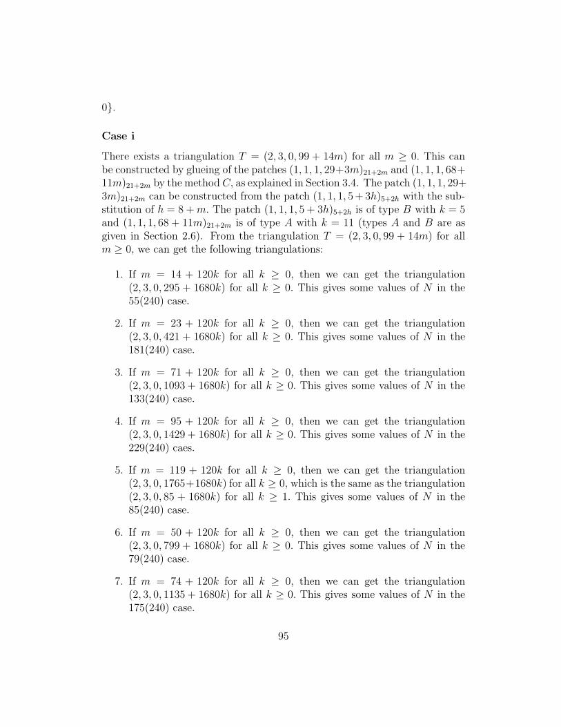
0}.
Case i
There exists a triangulation T = (2, 3, 0, 99 + 14m) for all m ≥ 0. This canbe constructed by glueing of the patches (1, 1, 1, 29+3m)21+2m and (1, 1, 1, 68+11m)21+2m by the method C, as explained in Section 3.4. The patch (1, 1, 1, 29+3m)21+2m can be constructed from the patch (1, 1, 1, 5+ 3h)5+2h with the sub-stitution of h = 8 +m. The patch (1, 1, 1, 5 + 3h)5+2h is of type B with k = 5and (1, 1, 1, 68 + 11m)21+2m is of type A with k = 11 (types A and B are asgiven in Section 2.6). From the triangulation T = (2, 3, 0, 99 + 14m) for allm ≥ 0, we can get the following triangulations:
1. If m = 14 + 120k for all k ≥ 0, then we can get the triangulation(2, 3, 0, 295 + 1680k) for all k ≥ 0. This gives some values of N in the55(240) case.
2. If m = 23 + 120k for all k ≥ 0, then we can get the triangulation(2, 3, 0, 421 + 1680k) for all k ≥ 0. This gives some values of N in the181(240) case.
3. If m = 71 + 120k for all k ≥ 0, then we can get the triangulation(2, 3, 0, 1093 + 1680k) for all k ≥ 0. This gives some values of N in the133(240) case.
4. If m = 95 + 120k for all k ≥ 0, then we can get the triangulation(2, 3, 0, 1429 + 1680k) for all k ≥ 0. This gives some values of N in the229(240) caes.
5. If m = 119 + 120k for all k ≥ 0, then we can get the triangulation(2, 3, 0, 1765+1680k) for all k ≥ 0, which is the same as the triangulation(2, 3, 0, 85 + 1680k) for all k ≥ 1. This gives some values of N in the85(240) case.
6. If m = 50 + 120k for all k ≥ 0, then we can get the triangulation(2, 3, 0, 799 + 1680k) for all k ≥ 0. This gives some values of N in the79(240) case.
7. If m = 74 + 120k for all k ≥ 0, then we can get the triangulation(2, 3, 0, 1135 + 1680k) for all k ≥ 0. This gives some values of N in the175(240) case.
95

8. If m = 110 + 120k for all k ≥ 0, then we can get the triangulation(2, 3, 0, 1639 + 1680k) for all k ≥ 0. This gives some values of N in the199(240) case.
Case ii
There exists a triangulation T = (2, 3, 0, 257 + 28m) for all m ≥ 0. Thiscan be constructed by glueing of the patches (1, 1, 1, 161 + 15m)25+2m and(1, 1, 1, 94 + 13m)25+2m by the method C, as explained in Section 3.4. Thepatch (1, 1, 1, 161+15m)25+2m can be constructed from the patch (1, 1, 1, 71+15h)13+2h with the substitution of h = 6+m. The patch (1, 1, 1, 71+15h)13+2h
is of type C with k = 13 and (1, 1, 1, 94+ 13m)25+2m is of type A with k = 13(types A and C are as given in Section 2.6). From the triangulation T =(2, 3, 0, 257 + 28m) for all m ≥ 0, we can get the following triangulations:
1. If m = 11 + 60k for all k ≥ 0, then we can get the triangulation(2, 3, 0, 565 + 1680k) for all k ≥ 0. This gives some values of N in the85(240) case.
2. If m = 23 + 60k for all k ≥ 0, then we can get the triangulation(2, 3, 0, 901 + 1680k) for all k ≥ 0. This gives some values of N in the181(240) case.
3. If m = 47 + 60k for all k ≥ 0, then we can get the triangulation(2, 3, 0, 1573 + 1680k) for all k ≥ 0. This gives some values of N inthe 133(240) case.
4. If m = 59 + 60k for all k ≥ 0, then we can get the triangulation(2, 3, 0, 1909 + 1680k) for all k ≥ 0, which is the same as the trian-gulation (2, 3, 0, 229 + 1680k) for all k ≥ 1. This gives some values of Nin the 229(240) case.
Case iii
There exists a triangulation T = (2, 3, 0, 143 + 28m) for all values of m ≥ 0.This can be constructed by glueing of the patches (1, 1, 1, 57+ 11m)13+2m and(1, 1, 1, 71+15m)13+2m by the method A, as explained in Section 3.4. The patch(1, 1, 1, 57+11m)13+2m can be constructed from the patch (1, 1, 1, 24+11h)7+2h
with the substitution of h = 3+m. The patch (1, 1, 1, 24+11h)7+2h is of type Dwith k = 7 and (1, 1, 1, 71+ 15m)13+2m is of type C with k = 13 (types C and
96
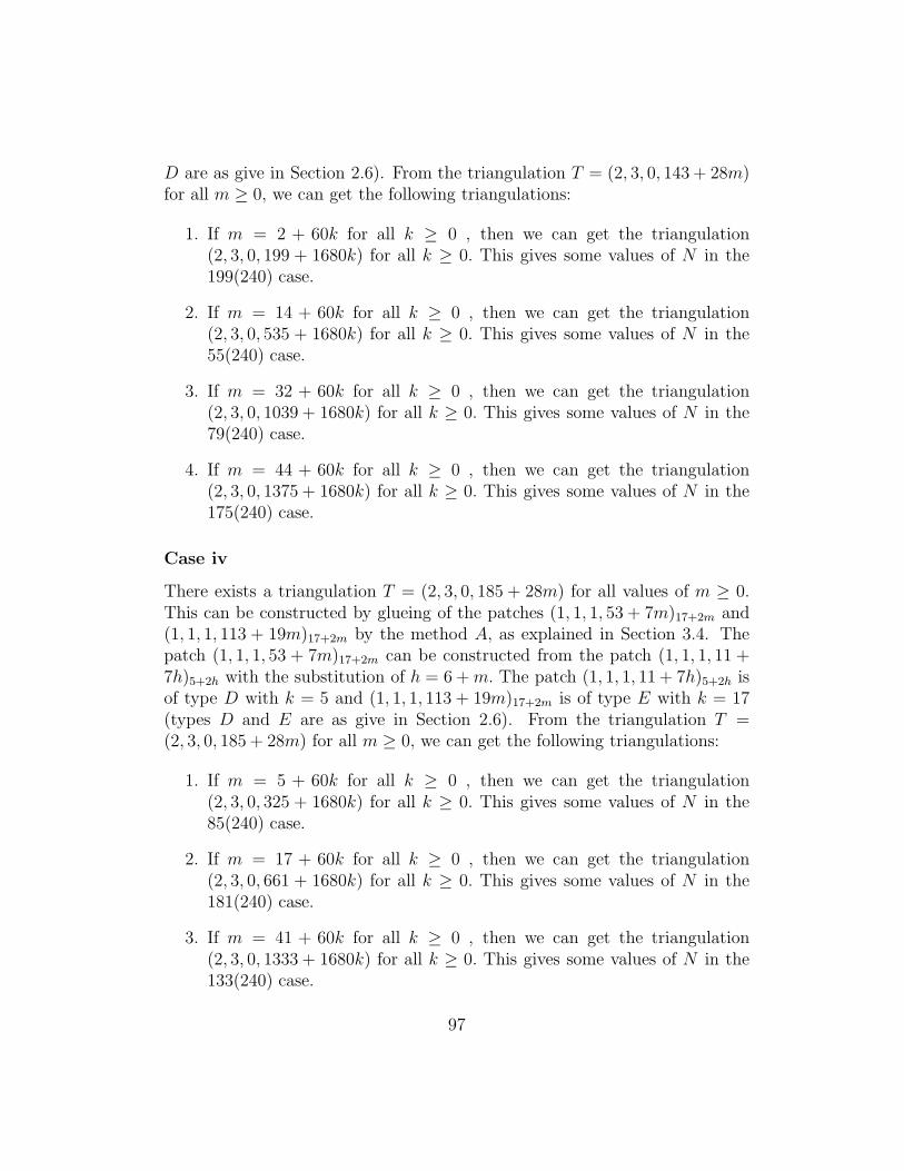
D are as give in Section 2.6). From the triangulation T = (2, 3, 0, 143 + 28m)for all m ≥ 0, we can get the following triangulations:
1. If m = 2 + 60k for all k ≥ 0 , then we can get the triangulation(2, 3, 0, 199 + 1680k) for all k ≥ 0. This gives some values of N in the199(240) case.
2. If m = 14 + 60k for all k ≥ 0 , then we can get the triangulation(2, 3, 0, 535 + 1680k) for all k ≥ 0. This gives some values of N in the55(240) case.
3. If m = 32 + 60k for all k ≥ 0 , then we can get the triangulation(2, 3, 0, 1039 + 1680k) for all k ≥ 0. This gives some values of N in the79(240) case.
4. If m = 44 + 60k for all k ≥ 0 , then we can get the triangulation(2, 3, 0, 1375 + 1680k) for all k ≥ 0. This gives some values of N in the175(240) case.
Case iv
There exists a triangulation T = (2, 3, 0, 185 + 28m) for all values of m ≥ 0.This can be constructed by glueing of the patches (1, 1, 1, 53 + 7m)17+2m and(1, 1, 1, 113 + 19m)17+2m by the method A, as explained in Section 3.4. Thepatch (1, 1, 1, 53 + 7m)17+2m can be constructed from the patch (1, 1, 1, 11 +7h)5+2h with the substitution of h = 6 +m. The patch (1, 1, 1, 11 + 7h)5+2h isof type D with k = 5 and (1, 1, 1, 113 + 19m)17+2m is of type E with k = 17(types D and E are as give in Section 2.6). From the triangulation T =(2, 3, 0, 185 + 28m) for all m ≥ 0, we can get the following triangulations:
1. If m = 5 + 60k for all k ≥ 0 , then we can get the triangulation(2, 3, 0, 325 + 1680k) for all k ≥ 0. This gives some values of N in the85(240) case.
2. If m = 17 + 60k for all k ≥ 0 , then we can get the triangulation(2, 3, 0, 661 + 1680k) for all k ≥ 0. This gives some values of N in the181(240) case.
3. If m = 41 + 60k for all k ≥ 0 , then we can get the triangulation(2, 3, 0, 1333 + 1680k) for all k ≥ 0. This gives some values of N in the133(240) case.
97

4. If m = 53 + 60k for all k ≥ 0 , then we can get the triangulation(2, 3, 0, 1669 + 1680k) for all k ≥ 0. This gives some values of N in the229(240) case.
Case v
There exists a triangulation T = (2, 3, 0, 167+28m) for all m ≥ 0. This can beconstructed by glueing of the patches (1, 1, 1, 46+9m)17+2m and (1, 1, 1, 119+19m)17+2m by the method C, as explained in Section 3.4. The patch (1, 1, 1,119+19m)17+2m can be constructed from the patch (1, 1, 1, 100 + 19h)15+2h withthe substitution of h = 1 + m. The patch (1, 1, 1, 100 + 19h)15+2h is of typeC with k = 15 and the patch (1, 1, 1, 46 + 9m)17+2m is of type A with k = 9(types A and C are as given in Section 2.6). From the triangulation T =(2, 3, 0, 167 + 28m) for all m ≥ 0, we can get the following triangulations:
1. If m = 14 + 60k for all k ≥ 0, then we can get the triangulation(2, 3, 0, 559 + 1680k) for all k ≥ 0. This gives some values of N in the79(240) case.
2. If m = 26 + 60k for all k ≥ 0, then we can get the triangulation(2, 3, 0, 895 + 1680k) for all k ≥ 0. This gives some values of N in the175(240) case.
3. If m = 44 + 60k for all k ≥ 0, then we can get the triangulation(2, 3, 0, 1399 + 1680k) for all k ≥ 0. This gives some values of N inthe 199(240) case.
4. If m = 56 + 60k for all k ≥ 0, then we can get the triangulation(2, 3, 0, 1735 + 1680k) for all k ≥ 0, which is the same as the trian-gulation (2, 3, 0, 55 + 1680k) for all k ≥ 1. This gives some values of Nin the 55(240) case.
Case vi
There exists a triangulation T = (2, 3, 0, 263+28m) for all m ≥ 0. This can beconstructed by glueing of the patches (1, 1, 1, 35+3m)25+2m and (1, 1, 1, 201+23m)25+2m by the method A, as explained in Section 3.4. The patch (1, 1, 1, 35+3m)25+2m can be constructed from the patch (1, 1, 1, 2+ 3h)3+2h with the sub-stitution of h = 11+m. The patch (1, 1, 1, 2+3h)3+2h is of type D with k = 3and (1, 1, 1, 201 + 23m)25+2m is of type F with k = 25 (types D and F are as
98

given in Section 2.6). From the triangulation T = (2, 3, 0, 263 + 28m) for allm ≥ 0, we can get the following triangulations:
1. Ifm = 2+60k for all k ≥ 0, then we can get the triangulation (2, 3, 0, 319+1680k) for all k ≥ 0. This gives some values of N in the 79(240) case.
2. If m = 14 + 60k for all k ≥ 0, then we can get the triangulation(2, 3, 0, 655 + 1680k) for all k ≥ 0. This gives some values of N in the175(240) case.
3. If m = 32 + 60k for all k ≥ 0, then we can get the triangulation(2, 3, 0, 1159 + 1680k) for all k ≥ 0. This gives some values of N inthe 199(240) case.
4. If m = 44 + 60k for all k ≥ 0, then we can get the triangulation(2, 3, 0, 1495 + 1680k) for all k ≥ 0. This gives some values of N inthe 55(240) case.
Case vii
There exists a triangulation T = (2, 3, 0, 147+28m) for all m ≥ 0. This can beconstructed by glueing of the patches (1, 1, 1, 20+3m)15+2m and (1, 1, 1, 110+23m)15+2m by the method A, as explained in Section 3.4. The patch (1, 1, 1, 20+3m)15+2m can be constructed from the patch (1, 1, 1, 5+3h)5+2h with the substi-tution of h = 5+m. The patches (1, 1, 1, 5+3h)5+2h and (1, 1, 1, 110+23m)15+2m
are of type B with k = 5 and k = 15 respectively (type B is as given in Section2.6). From the triangulation T = (2, 3, 0, 147+28m) for all m ≥ 0, we can getthe following triangulations:
1. Ifm = 1+60k for all k ≥ 0, then we can get the triangulation (2, 3, 0, 175+1680k) for all k ≥ 0. This gives some values of N in the 175(240) case.
2. If m = 19 + 60k for all k ≥ 0, then we can get the triangulation(2, 3, 0, 679 + 1680k) for all k ≥ 0. This gives some values of N in the199(240) case.
3. If m = 31 + 60k for all k ≥ 0, then we can get the triangulation(2, 3, 0, 1015 + 1680k) for all k ≥ 0. This gives some values of N inthe 55(240) case.
99

4. If m = 49 + 60k for all k ≥ 0, then we can get the triangulation(2, 3, 0, 1519 + 1680k) for all k ≥ 0. This gives some values of N inthe 79(240) case.
Case viii
There exists a triangulation T = (2, 3, 0, 135 + 28m) for all m ≥ 0. This canbe constructed by glueing of the patches (1, 1, 1, 39+7m)13+2m and (1, 1, 1, 81+19m)13+2m by the method A, as explained in Section 3.4. The patch (1, 1, 1, 39+7m)13+2m can be constructed from the patch (1, 1, 1, 11+7h)5+2h with the sub-stitution of h = 4+m. The patch (1, 1, 1, 11+7h)5+2h is of type D with k = 5and (1, 1, 1, 81 + 19m)13+2m is of type C with k = 13 (types C and D are asgiven in Section 2.6). From the triangulation T = (2, 3, 0, 135 + 28m) for allm ≥ 0, we can get the following triangulations:
1. If m = 10 + 60k for all k ≥ 0, then we can get the triangulation(2, 3, 0, 415 + 1680k) for all k ≥ 0. This gives some values of N in the175(240) case.
2. If m = 28 + 60k for all k ≥ 0, then we can get the triangulation(2, 3, 0, 919 + 1680k) for all k ≥ 0. This gives some values of N in the199(240) case.
3. If m = 40 + 60k for all k ≥ 0, then we can get the triangulation(2, 3, 0, 1255 + 1680k) for all k ≥ 0. This gives some values of N inthe 55(240) case.
4. If m = 58 + 60k for all k ≥ 0, then we can get the triangulation(2, 3, 0, 1759 + 1680k) for all k ≥ 0, which is the same as the trian-gulation (2, 3, 0, 79 + 1680k) for all k ≥ 1. This gives some values of Nin the 79(240) case.
Case ix
There exists a triangulation T = (2, 3, 0, 159 + 28m) for all m ≥ 0. Thiscan be constructed by glueing of the patches (1, 1, 1, 62 + 11m)15+2m and(1, 1, 1, 80+15m)15+2m by the method A, as explained in Section 3.4. The patch(1, 1, 1, 62+11m)15+2m can be constructed from the patch (1, 1, 1, 51+11h)13+2h
with the substitution of h = 1 + m. The patches (1, 1, 1, 51 + 11h)13+2h and(1, 1, 1, 80+15m)15+2m are of type E with k = 13 and k = 15 respectively (type
100

E is as given in Section 2.6). From the triangulation T = (2, 3, 0, 159 + 28m)for all m ≥ 0, we can get the following triangulations:
1. If m = 40 + 60k for all k ≥ 0, then we can get the triangulation(2, 3, 0, 1279 + 1680k) for all k ≥ 0. This gives some values of N inthe 79(240) case.
2. If m = 52 + 60k for all k ≥ 0, then we can get the triangulation(2, 3, 0, 1615 + 1680k) for all k ≥ 0. This gives some values of N inthe 175(240) case.
3. If m = 10 + 60k for all k ≥ 0, then we can get the triangulation(2, 3, 0, 439 + 1680k) for all k ≥ 0. This gives some values of N in the199(240) case.
4. If m = 22 + 60k for all k ≥ 0, then we can get the triangulation(2, 3, 0, 775 + 1680k) for all k ≥ 0. This gives some values of N in the55(240) case.
Case x
There exists a triangulation T = (2, 3, 0, 377 + 28m) for all m ≥ 0. Thiscan be constructed by glueing of the patches (1, 1, 1, 238 + 21m)41+2m and(1, 1, 1, 137+7m)41+2m by the method C, as explained in Section 3.4. The patch(1, 1, 1, 137+7m)41+2m can be constructed from the patch (1, 1, 1, 18+7h)7+2h
with the substitution of h = 17+m. The patch (1, 1, 1, 18+7h)7+2h is of type Bwith k = 7 and (1, 1, 1, 238+21m)41+2m is of type A with k = 21 (types A andB are as given in Section 2.6). From the triangulation T = (2, 3, 0, 377+28m)for all m ≥ 0, we can get the following triangulations:
1. If m = 17 + 60k for all k ≥ 0, then we can get the triangulation(2, 3, 0, 853 + 1680k) for all k ≥ 0. This gives some values of N in the133(240) case.
2. If m = 29 + 60k for all k ≥ 0, then we can get the triangulation(2, 3, 0, 1189 + 1680k) for all k ≥ 0. This gives some values of N inthe 229(240) case.
3. If m = 41 + 60k for all k ≥ 0, then we can get the triangulation(2, 3, 0, 1525 + 1680k) for all k ≥ 0. This gives some values of N inthe 85(240) case.
101

4. If m = 53 + 60k for all k ≥ 0, then we can get the triangulation(2, 3, 0, 1861 + 1680k) for all k ≥ 0, which is the same as the trian-gulation (2, 3, 0, 181 + 1680k) for all k ≥ 1. This gives some values of Nin the 181(240) case.
Case xi
There exists a triangulation T = (2, 3, 0, 137 + 28m) for all m ≥ 0. Thiscan be constructed by glueing of the patches (1, 1, 1, 51 + 11m)13+2m and(1, 1, 1, 71+15m)13+2m by the method A, as explained in Section 3.4. The patch(1, 1, 1, 51+11m)13+2m is of type E with k = 13 and (1, 1, 1, 71+15m)13+2m isof type C with k = 13 (types C and E are as given in Section 2.6). From thetriangulation T = (2, 3, 0, 137 + 28m) for all m ≥ 0, we can get the followingtriangulations:
1. If m = 17 + 60k for all k ≥ 0, then we can get the triangulation(2, 3, 0, 613 + 1680k) for all k ≥ 0. This gives some values of N in the133(240) case.
2. If m = 29 + 60k for all k ≥ 0, then we can get the triangulation(2, 3, 0, 949 + 1680k) for all k ≥ 0. This gives some values of N in the229(240) case.
3. If m = 41 + 60k for all k ≥ 0, then we can get the triangulation(2, 3, 0, 1285 + 1680k) for all k ≥ 0. This gives some values of N inthe 85(240) case.
4. If m = 53 + 60k for all k ≥ 0, then we can get the triangulation(2, 3, 0, 1621 + 1680k) for all k ≥ 0. This gives some values of N inthe 181(240) case.
Case xii
There exists a triangulation T = (2, 3, 0, 161+28m) for all m ≥ 0. This can beconstructed by glueing of the patches (1, 1, 1, 46+9m)17+2m and (1, 1, 1, 113+19m)17+2m by the method C, as explained in Section 3.4. The patch (1, 1, 1, 46+9m)17+2m is of type A with k = 9 and (1, 1, 1, 113+19m)17+2m is of type E withk = 17 (types A and E are as given in Section 2.6). From the triangulationT = (2, 3, 0, 161+ 28m) for all m ≥ 0, we can get the following triangulations:
102

1. If m = 59 + 60k for all k ≥ 0, then we can get the triangulation(2, 3, 0, 1813 + 1680k) for all k ≥ 0, which is the same as the trian-gulation (2, 3, 0, 133+ 1680k) for all k ≥ 1. This gives some values of Nin the 133(240) case.
2. If m = 23 + 60k for all k ≥ 0, then we can get the triangulation(2, 3, 0, 805 + 1680k) for all k ≥ 0. This gives some values of N in the85(240) case.
3. If m = 11 + 60k for all k ≥ 0, then we can get the triangulation(2, 3, 0, 469 + 1680k) for all k ≥ 0. This gives some values of N in the229(240) case.
4. If m = 35 + 60k for all k ≥ 0, then we can get the triangulation(2, 3, 0, 1141 + 1680k) for all k ≥ 0. This gives some values of N inthe 181(240) case.
Case xiii
There exists a triangulation T = (2, 3, 0, 233 + 28m) for all m ≥ 0. Thiscan be constructed by glueing of the patches (1, 1, 1, 94 + 13m)25+2m and(1, 1, 1, 137 + 15m)25+2m by the method C, as explained in Section 3.4. Thepatch (1, 1, 1, 137+15m)25+2m can be constructed from the patch (1, 1, 1, 107+15h)21+2h with the substitution of h = 2+m. The patch (1, 1, 1, 107+15h)21+2h
is of type F with k = 21 and (1, 1, 1, 94 + 13m)25+2m is of type A withk = 13 (types A and F are as given in Section 2.6). From the triangulationT = (2, 3, 0, 233+ 28m) for all m ≥ 0, we can get the following triangulations:
1. If m = 29 + 60k for all k ≥ 0, then we can get the triangulation(2, 3, 0, 1045 + 1680k) for all k ≥ 0. This gives some values of N inthe 85(240) case.
2. Ifm = 5+60k for all k ≥ 0, then we can get the triangulation (2, 3, 0, 373+1680k) for all k ≥ 0. This gives some values of N in the 133(240) case.
3. If m = 41 + 60k for all k ≥ 0, then we can get the triangulation(2, 3, 0, 1381 + 1680k) for all k ≥ 0. This gives some values of N inthe 181(240) case.
4. If m = 17 + 60k for all k ≥ 0, then we can get the triangulation(2, 3, 0, 709 + 1680k) for all k ≥ 0. This gives some values of N in the229(240) case.
103

From the above 13 cases we found triangulations for all values of N in N ′
except for the values 55, 79, 85, 181, 229. We can construct the triangulationsfor these values as follows:
1. The triangulation (2, 3, 0, 55) exists. This can be constructed by glue-ing of the patches (1, 1, 1, 19)9 and (1, 1, 1, 25)9 by the method A, asexplained in Section 3.4. The patch (1, 1, 1, 19)9 is of type M with k = 9and (1, 1, 1, 25)9 is of type L with k = 9 (types M and L are as given inSection 2.6).
2. The triangulation (2, 3, 0, 79) exists. This can be constructed by glueingof the patches (1, 1, 1, 26)11 and (1, 1, 1, 40)11 by the method A, as ex-plained in Section 3.4. The patch (1, 1, 1, 26)11 is of type O with k = 11and (1, 1, 1, 40)11 is of type M with k = 11 (types O and M are as givenin Section 2.6).
3. The triangulation (2, 3, 0, 85) exists. This can be constructed by glueingof the patch (1, 1, 1, 37)9 with itself (that is, (1, 1, 1, 37)9 and (1, 1, 1, 37)9)by the method A, as explained in Section 3.4. The patch (1, 1, 1, 37)9 isof type I with k = 9 (type I is as given in Section 2.6).
4. The triangulation (2, 3, 0, 181) exists. This can be constructed by glueingof the patch (1, 1, 1, 83)13 with itself (that is, (1, 1, 1, 83)13 and (1, 1, 1,83)13) by the method A, as explained in Section 3.4. The patch (1, 1, 1,83)13 is of type I with k = 13 (type I is as given in Section 2.6).
5. The triangulation (2, 3, 0, 229) exists. This can be constructed by glue-ing of the patches (1, 1, 1, 31)23 and (1, 1, 1, 196)23 by the method B,as explained in Section 3.4. The patch (1, 1, 1, 31)23 is of type A withk = 3, m = 9 and (1, 1, 1, 196)23 is of type E with k = 19, m = 2 (typesA and E are as given in Section 2.6).
3.20.3 3(6) type
To construct this type, we will consider the triangulations of the form (2, 3, 0,X + Y m) with Y = 6, 12, 18, 24, 30, 36 and all possible values of X. Theleast common multiple of 6, 12, 18, 24, 30, 36 is 360. Therefore the valuesof N to consider in this 3(6) type are {3 + Y m | 3 + Y m ≤ 360, Y =6, 12, 18, 24, 30, 36; m ≥ 0}. For the constructions we will consider the fol-lowing cases:
104

Case 1
The triangulation (2, 3, 0, 21 + 12m) exists for all m ≥ 0, by glueing of thepatches (0, 3, 0, 16)12 and (2, 0, 0, 5)12. The patch (0, 3, 0, 16)12 can be con-structed from the patch given in Theorem 2.2.1(iii) with h = 4, k = 2 andthe patch (2, 0, 0, 5)12 is a special case of patches of the type (2, 0, 0) withk = 6, r = 0 (as discussed in Section 2.1).
Case 2
The triangulation (2, 3, 0, 33 + 18m) exists for all m ≥ 0, by glueing of thepatches (0, 3, 0, 25)18 and (2, 0, 0, 8)18. The patch (0, 3, 0, 25)18 can be con-structed from the patch given in Theorem 2.2.1(ii) with h = 6 and the patch(2, 0, 0, 8)18 is a special case of patches of the type (2, 0, 0) with k = 9, r = 0(as discussed in Section 2.1).
Case 3
The triangulation (2, 3, 0, 57 + 18m) exists for all m ≥ 0, by glueing of thepatches (0, 3, 0, 49)18 and (2, 0, 0, 8)18. The patch (0, 3, 0, 49)18 can be con-structed from the patch given in Theorem 2.2.1(iv) with h = 6, k = 4, l = 2and the patch (2, 0, 0, 8)18 is a special case of patches of the type (2, 0, 0) withk = 9, r = 0 (as discussed in Section 2.1).
Case 4
The triangulation (2, 3, 0, 93 + 30m) exists for all m ≥ 0, by glueing of thepatches (0, 3, 0, 79)30 and (2, 0, 0, 14)30. The patch (0, 3, 0, 79)30 can be con-structed from the patch given in Theorem 2.2.1(iii) with h = 10, k = 2 andthe patch (2, 0, 0, 14)30 is a special case of patches of the type (2, 0, 0) withk = 15, r = 0 (as discussed in Section 2.1).
Case 5
The triangulation (2, 3, 0, 141 + 30m) exists for all m ≥ 0, by glueing of thepatches (0, 3, 0, 127)30 and (2, 0, 0, 14)30. The patch (0, 3, 0, 127)30 can be con-structed from the patch given in Theorem 2.2.1(iv) with h = 10, k = 4, l = 4and the patch (2, 0, 0, 14)30 is a special case of patches of the type (2, 0, 0) withk = 15, r = 0 (as discussed in Section 2.1).
105

Case 6
The triangulation (2, 3, 0, 129 + 30m) exists for all m ≥ 0, by glueing of thepatches (0, 3, 0, 115)30 and (2, 0, 0, 14)30. The patch (0, 3, 0, 115)30 can be con-structed from the patch given in Theorem 2.2.1(iv) with h = 10, k = 6, l = 2and the patch (2, 0, 0, 14)30 is a special case of patches of the type (2, 0, 0) withk = 15, r = 0 (as discussed in Section 2.1).
Case 7
The triangulation (2, 3, 0, 165 + 30m) exists for all m ≥ 0, by glueing of thepatches (0, 3, 0, 151)30 and (2, 0, 0, 14)30. The patch (0, 3, 0, 151)30 can be con-structed from the patch given in Theorem 2.2.1(iv) with h = 10, k = 8, l = 6and the patch (2, 0, 0, 14)30 is a special case of patches of the type (2, 0, 0) withk = 15, r = 0 (as discussed in Section 2.1).
From the above seven cases, we found triangulations of the type (2, 3, 0, N)for all N ≡ 3(6) except for the case N ≡ 27(180) and the values N =3, 9, 15, 39, 63, 99, 135. We next find triangulations for the case N ≡ 27(180).To do this, we will consider the following cases:
Case (i)
The triangulation T = (2, 3, 0, 27 + 1260m) exists for all m ≥ 1. This can beconstructed as follows:Glueing of the patches (0, 3, 0, 301)42 and (2, 0, 0, 20)42 gives a triangulationT1 = (2, 3, 0, 321 + 42h) for h ≥ 0. The patch (2, 0, 0, 20)42 is a special caseof patches of the type (2, 0, 0) with k = 21, r = 0 (as discussed in Section2.1) and the patch (0, 3, 0, 301)42 is as given in Theorem 2.2.1(iv) with h =14, k = 12, l = 10. If we substitute h = 23 + 30m in the triangulation T1 =(2, 3, 0, 321 + 42h), then we can get the triangulation (2, 3, 0, 1287 + 1260m)for m ≥ 0 which is the same as the triangulation T = (2, 3, 0, 27 + 1260m)for m ≥ 1. The triangulation T gives all the values of the 27(1260) case,except the initial value 27. For N = 27 the triangulation (2, 3, 0, 27) can beconstructed as follows:Glueing of the patches (1, 1, 1, 4 + 3m)5+2m and (1, 1, 1, 11 + 7m)5+2m by themethod C, as explained in Section 3.4, gives a triangulation (2, 3, 0, 17+10m)for m ≥ 0. If m = 1, then we can get the triangulation (2, 3, 0, 27). The patch
106
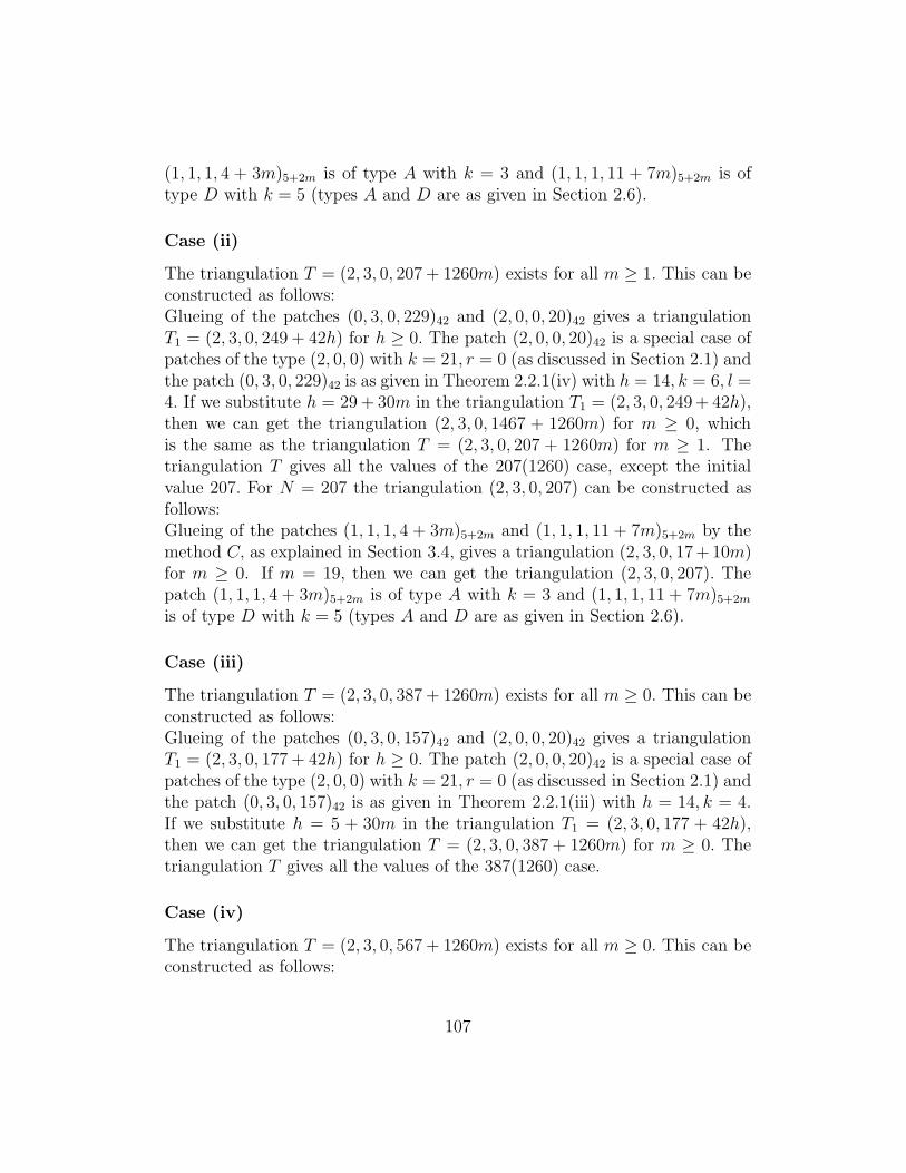
(1, 1, 1, 4 + 3m)5+2m is of type A with k = 3 and (1, 1, 1, 11 + 7m)5+2m is oftype D with k = 5 (types A and D are as given in Section 2.6).
Case (ii)
The triangulation T = (2, 3, 0, 207 + 1260m) exists for all m ≥ 1. This can beconstructed as follows:Glueing of the patches (0, 3, 0, 229)42 and (2, 0, 0, 20)42 gives a triangulationT1 = (2, 3, 0, 249 + 42h) for h ≥ 0. The patch (2, 0, 0, 20)42 is a special case ofpatches of the type (2, 0, 0) with k = 21, r = 0 (as discussed in Section 2.1) andthe patch (0, 3, 0, 229)42 is as given in Theorem 2.2.1(iv) with h = 14, k = 6, l =4. If we substitute h = 29+ 30m in the triangulation T1 = (2, 3, 0, 249+ 42h),then we can get the triangulation (2, 3, 0, 1467 + 1260m) for m ≥ 0, whichis the same as the triangulation T = (2, 3, 0, 207 + 1260m) for m ≥ 1. Thetriangulation T gives all the values of the 207(1260) case, except the initialvalue 207. For N = 207 the triangulation (2, 3, 0, 207) can be constructed asfollows:Glueing of the patches (1, 1, 1, 4 + 3m)5+2m and (1, 1, 1, 11 + 7m)5+2m by themethod C, as explained in Section 3.4, gives a triangulation (2, 3, 0, 17+10m)for m ≥ 0. If m = 19, then we can get the triangulation (2, 3, 0, 207). Thepatch (1, 1, 1, 4 + 3m)5+2m is of type A with k = 3 and (1, 1, 1, 11 + 7m)5+2m
is of type D with k = 5 (types A and D are as given in Section 2.6).
Case (iii)
The triangulation T = (2, 3, 0, 387 + 1260m) exists for all m ≥ 0. This can beconstructed as follows:Glueing of the patches (0, 3, 0, 157)42 and (2, 0, 0, 20)42 gives a triangulationT1 = (2, 3, 0, 177 + 42h) for h ≥ 0. The patch (2, 0, 0, 20)42 is a special case ofpatches of the type (2, 0, 0) with k = 21, r = 0 (as discussed in Section 2.1) andthe patch (0, 3, 0, 157)42 is as given in Theorem 2.2.1(iii) with h = 14, k = 4.If we substitute h = 5 + 30m in the triangulation T1 = (2, 3, 0, 177 + 42h),then we can get the triangulation T = (2, 3, 0, 387 + 1260m) for m ≥ 0. Thetriangulation T gives all the values of the 387(1260) case.
Case (iv)
The triangulation T = (2, 3, 0, 567 + 1260m) exists for all m ≥ 0. This can beconstructed as follows:
107

Glueing of the patches (0, 3, 0, 169)42 and (2, 0, 0, 20)42 gives a triangulationT1 = (2, 3, 0, 189 + 42h) for h ≥ 0. The patch (2, 0, 0, 20)42 is a special case ofpatches of the type (2, 0, 0) with k = 21, r = 0 (as discussed in Section 2.1) andthe patch (0, 3, 0, 169)42 is as given in Theorem 2.2.1(iv) with h = 14, k = 2, l =2. If we substitute h = 9 + 30m in the triangulation T1 = (2, 3, 0, 189 + 42h),then we can get the triangulation T = (2, 3, 0, 567 + 1260m) for m ≥ 0. Thetriangulation T gives all the values of the 567(1260) case.
Case (v)
The triangulation T = (2, 3, 0, 747 + 1260m) exists for m ≥ 0. This can beconstructed as follows:Glueing of the patches (0, 3, 0, 265)42 and (2, 0, 0, 20)42 gives a triangulationT1 = (2, 3, 0, 285 + 42h) for h ≥ 0. The patch (2, 0, 0, 20)42 is a special case ofpatches of the type (2, 0, 0) with k = 21, r = 0 (as discussed in Section 2.1)and the patch (0, 3, 0, 265)42 is from the patch given in Theorem 2.2.1(iv) withh = 14, k = 10, l = 6. If we substitute h = 11+ 30m in the triangulation T1 =(2, 3, 0, 285+42h), then we can get the triangulation T = (2, 3, 0, 747+1260m)for m ≥ 0. The triangulation T gives all the values of the 747(1260) case.
Case (vi)
The triangulation T = (2, 3, 0, 927 + 1260m) exists for all m ≥ 0. This can beconstructed as follows:Glueing of the patches (0, 3, 0, 277)42 and (2, 0, 0, 20)42 gives a triangulationT1 = (2, 3, 0, 297 + 42h) for h ≥ 0. The patch (2, 0, 0, 20)42 is a special case ofpatches of the type (2, 0, 0) with k = 21, r = 0 (as discussed in Section 2.1)and the patch (0, 3, 0, 277)42 is from the patch given in Theorem 2.2.1(iv) withh = 14, k = 8, l = 8. If we substitute h = 15 + 30m in the triangulation T1 =(2, 3, 0, 297+42h), then we can get the triangulation T = (2, 3, 0, 927+1260m)for m ≥ 0. The triangulation T gives all the values of the 927(1260) case.
Case (vii)
The triangulation T = (2, 3, 0, 1107 + 1260m) exists for all m ≥ 0. This canbe constructed as follows:Glueing of the patches (0, 3, 0, 205)42 and (2, 0, 0, 20)42 gives a triangulationT1 = (2, 3, 0, 225 + 42h) for h ≥ 0. The patch (2, 0, 0, 20)42 is a special case ofpatches of the type (2, 0, 0) with k = 21, r = 0 (as discussed in Section 2.1) and
108

the patch (0, 3, 0, 205)42 is as given in Theorem 2.2.1(iv) with h = 14, k = 8, l =2. If we substitute h = 21+ 30m in the triangulation T1 = (2, 3, 0, 225+ 42h),then we can get the triangulation T = (2, 3, 0, 1107 + 1260m) for m ≥ 0. Thetriangulation T gives all the values of the 1107(1260) case.
Case (i) to (vii) above give triangulations for all the values of the 27(180)case. The remaining values of N to consider are N = 3, 9, 15, 39, 63, 99, 135.
1. The triangulation (2, 3, 0, 9) can be constructed as follows: Glueing ofthe patches (1, 1, 1, 2+3m)3+2m and (1, 1, 1, 2+ 3m)3+2m by the methodA, as explained in Section 3.4, gives a triangulation (2, 3, 0, 9 + 8m) form ≥ 0. If m = 0, then we can get the triangulation (2, 3, 0, 9). Thepatch (1, 1, 1, 2 + 3m)3+2m is of type D with k = 3 (type D is as givenin Section 2.6).
2. The triangulation (2, 3, 0, 39) can be constructed by glueing of the patches(1, 1, 1, 12)7 and (1, 1, 1, 18)7 by the method A, as explained in Section3.4. The patch (1, 1, 1, 12)7 is of type K with k = 7 and (1, 1, 1, 18)7 isof type J with k = 7 (types J and K are as given in Section 2.6).
3. The triangulation (2, 3, 0, 63) can be constructed by glueing of the patches(1, 1, 1, 11)9 and (1, 1, 1, 41)9 by the method A, as explained in Section3.4. The patch (1, 1, 1, 11)9 is given in Table 2.6 and (1, 1, 1, 41)9 is oftype H with k = 9 (type H is as given in Section 2.6).
4. The triangulation (2, 3, 0, 99) can be constructed by glueing of the patches(1, 1, 1, 40)11 and (1, 1, 1, 46)11 by the method A, as explained in Section3.4. The patch (1, 1, 1, 40)11 is of type M with k = 11 and (1, 1, 1, 46)11is of type L with k = 11 (types K and L are as given in Section 2.6).
5. The triangulation (2, 3, 0, 135) can be constructed by glueing of thepatches (1, 1, 1, 33)13 and (1, 1, 1, 87)13 by the method A, as explainedin Section 3.4. The patch (1, 1, 1, 33)13 is of type E with k = 11, m = 1and (1, 1, 1, 87)13 is of type H with k = 13 (types E and H are as givenin Section 2.6).
We have not been able to construct triangulations for the case N = 3, 15.
3.20.4 5(6) type
The triangulation T = (2, 3, 0, 5 + 6m) for all m ≥ 0 can be constructed byglueing of the patches (2, 0, 0, 2)6 and (0, 3, 0, 3)6. The patch (2, 0, 0, 2)6 is a
109

special case of patches of the type (2, 0, 0) with k = 3, r = 0 (as discussedin Section 2.1) and the patch (0, 3, 0, 3)6 is as given in Theorem 2.2.1(ii) withh = 2. The triangulation T gives all the values of the 5(6) type.
3.21 Triangulations of type (3, 0, 3)
In this section we show that the triangulation (3, 0, 3, N) exists for all valuesof N except for N = 0, 2 and possibly N = 4, 12.
N = a6 Triangulation1 {125, 127, 135, 136, 146, 147, 247, 235, 346, 234 }3 {123, 129, 138, 148, 145, 237, 256, 267, 259, 348, 346, 367,
159, 456 }6 {123, 134, 145, 15B, 12B, 237, 27C, 2AC, 2AB, 345, 356,
367, 569, 689, 678, 789, ABC, 59B, 79C, 9BC }8 {12B, 128, 15B, 15C, 189, 19C, 237, 23E, 27B, 28E, 348,
34A, 37A, 38E, 456, 459, 46A, 489, 56B, 59C, 67B, 67D,6AD, 7AD }
Table 3.17: Some triangulations of type (3, 0, 3)
To construct triangulations of this type we will consider two cases: (1) Nodd, (2) N even.
3.21.1 N odd
There exists a triangulation T : (3, 0, 3, 2m + 1) for all m ≥ 0. This can beconstructed as follows:
In Section 3.23 it will be shown that the triangulation T1 : (4, 0, 0, 2n) existsfor each n ≥ 2. This triangulation has a point of degree 3 adjacent to threepoints, say x, y, z of degree 6. If we remove this point of degree three, then thedegrees of the points x, y, z will become 5, that is, we will get three points ofdegree 5. Hence, we will get the triangulation T : (3, 0, 3, 2m+ 1) for m ≥ 0.
N even
In this case we will consider three types: 0(6), 2(6), 4(6).
110

3.21.2 0(6) type
To construct triangulations of this type, we will consider two sub-types: 0(12),6(12).
Case 1: 0(12) type
There exists a triangulation T : (3, 0, 3, 0 + 12m) for all m ≥ 3. This can beconstructed as follows:Glueing of the patches (1, 0, 3, 31)12 and (2, 0, 0, 5)12 gives a triangulation(3, 0, 3, 36 + 12m) for m ≥ 0, which is the same as the triangulation T :(3, 0, 3, 0 + 12m) for m ≥ 3. The patch (1, 0, 3, 31)12 can be constructedby using the edge-fullering construction on the patch (1, 0, 3, 7)6, that is,EF (1, 0, 3, 7)6 = (1, 0, 3, 31)12 where (1, 0, 3, 7)6 is given in Table 2.4.The patch(2, 0, 0, 5)12 is a special case of patches of the type (2, 0, 0) with k = 6, r = 0(as discussed in Section 2.1).
The triangulation T gives all the values of the 0(12) type, except the initialvalues N = 0, 12, 24. For N = 0, the triangulation cannot be constructed ashas been shown by Eberhard [3] and Bruckner [2] (see also Grunbaum [4]).We have not been able to construct a triangulation for the case N = 12. ForN = 24, the triangulation (3, 0, 3, 24) can be constructed by using the edge-fullering construction on the triangulation (3, 0, 3, 3), that is, EF (3, 0, 3, 3) =(3, 0, 3, 24). The construction of the triangulation (3, 0, 3, 3) is given in Table3.17.
Case2: 6(12) type
We will divide this type into two more sub-types: 6(24) and 18(24).
Case 2.1: 6(24) type
There exists a triangulation T : (3, 0, 3, 6 + 24m) for all m ≥ 1. This can beconstructed as follows:Glueing of the patches (1, 0, 3, 27)8 and (2, 0, 0, 3)8 gives a triangulation T1 :(3, 0, 3, 30 + 8h) for h ≥ 0. If h = 3m, then we can get the triangulation(3, 0, 3, 30 + 24m) for m ≥ 0, which is the same as the triangulation T :(3, 0, 3, 6 + 24m) for m ≥ 1. The patch (1, 0, 3, 27)8 can be constructed byusing the generic construction method for β5 = 1 three times on the patch(1, 0, 3, 6)5. The patch (1, 0, 3, 6)5 is given in Table 2.3 whereas the patch(2, 0, 0, 3)8 is a special case of patches of the type (2, 0, 0) with k = 4, r = 0
111

(as discussed in Section 2.1). The triangulation T gives all the values of the6(24) type, except the initial value of N = 6. For N = 6, the triangulation isgiven in Table 3.17 above.
Case 2.2: 18(24) type
There exists a triangulation T : (3, 0, 3, 18 + 24m) for all m ≥ 0. This can beconstructed as follows:Glueing of the patches (1, 0, 3, 15)8 and (2, 0, 0, 3)8 gives a triangulation T1 :(3, 0, 3, 18 + 8h) for h ≥ 0. If h = 3m, then we can get the triangulationT : (3, 0, 3, 18 + 24m) for m ≥ 0. The construction of the patch (1, 0, 3, 15)8is given in Table 2.6 and (2, 0, 0, 3)8 is a special case of patches of the type(2, 0, 0) with k = 4, r = 0 (as discussed in Section 2.1). The triangulation Tgives all the values of the 18(24) type.
3.21.3 2(6) type
There exists a triangulation T : (3, 0, 3, 2 + 6m) for all m ≥ 1. This can beconstructed as follows:Glueing of the patches (1, 0, 3, 12)6 and (2, 0, 0, 2)6 gives a triangulation T1 :(3, 0, 3, 14 + 6m) for m ≥ 0, which is the same as the triangulation T :(3, 0, 3, 2 + 6m) for m ≥ 2. The patch (1, 0, 3, 12)6 can be constructed fromthe patch (1, 0, 3, 6)5 by using the generic construction method with β5 = 1.The patch (1, 0, 3, 6)5 is given in Table 2.3 whereas (2, 0, 0, 2)6 is a special caseof patches of the type (2, 0, 0) with k = 3, r = 0 (as discussed in Section 2.1).The triangulation T gives all the values of the 2(6) type, except the two initialvalues of N = 2, 8. For N = 8, the triangulation is given in Table 3.17 above.For N = 2, the triangulation (3, 0, 3, 2) cannot be constructed. We can arguethis as follows:
Let X = {abcdefg} with the triangles abc, acd, ade, aef, afg, abg and letthe degree of the point a be d(a) = 6.
Case (I): Suppose that the points b, c, d, e, f, g all have degree < 6. If a pointh of degree 6 is included in this construction, then we may assume (withoutloss of generality) that h is adjacent to e and d, and there must be 5 moretriangles hfg, hef, hcd, hbc, hbg. But then the points b, c, d, e, f, g will havedegree 4. Thus the triangulation (3, 0, 3, 2) cannot be constructed in this case.
112

Case (II): Suppose without loss of generality that the point e has degree 6.Let h be another point to be added to this construction (so that h has degree3 or 5). Suppose first that h is adjacent to e. Without loss of generality, wemay assume that hed forms a triangle. Since h has degree 3 or 5 and we donot want to add any new points to this construction, the point e will end uphaving degree 3 or 4; a contradiction. Suppose now that h is not adjacent toe. Again, since h has degree 3 or 5 and we do not want to add any new pointsto this construction, the point e will end up having degree 2, 3 or 4 which isalso a contradiction.
Hence the triangulation (3, 0, 3, 2) cannot be constructed.
3.21.4 4(6) type
There exists a triangulation T : (3, 0, 3, 4 + 6m) for all m ≥ 1. This can beconstructed as follows:Glueing of the patches (1, 0, 3, 8)6 and (2, 0, 0, 2)6 gives a triangulation (3, 0, 3,10 + 6h) for h ≥ 0, which is the same as the triangulation T : (3, 0, 3, 4 + 6m)for m ≥ 1. The construction of the patch (1, 0, 3, 8)6 is given in Table 2.4 and(2, 0, 0, 2)6 is a special case of patches of the type (2, 0, 0) with k = 3, r = 0(as discussed in Section 2.1).
The triangulation T gives all the values of the 4(6) type, except the initialvalue of N = 4. We have not been able to construct a triangulation for thecase N = 4.
3.22 Triangulations of type (3, 1, 1)
It is known by Grunbaum and Motzkin [5] (see also [4]) that the triangulation(3, 1, 1, 2m) does not exist for all m ≥ 0. In this section we show that thetriangulation (3, 1, 1, N) exists for all odd values of N except for N = 1 andpossibly N = 17. We will consider two types: 1(4) and 3(4).
3.22.1 1(4) type
To construct triangulations of this type, we will consider two sub-types: 1(8)and 5(8).
113

N = a6 Triangulation3 {124, 126, 135, 145, 138, 168, 235, 245, 237, 267, 367, 368 }5 {123, 126, 137, 158, 178, 156, 239, 249, 24A, 26A, 349,
345, 357, 456, 46A, 578 }9 {124, 12C, 134, 13B, 1AC, 1AB, 234, 235, 25C, 357, 37B,
568, 56C, 587, 678, 679, 69D, 6CD, 79B, 9AE, 9BE, 9AD,AEB, ACD }
Table 3.18: Some triangulations of type (3, 1, 1)
1(8) type
We will divide this type into three sub-types, namely, 1(24), 9(24), 17(24).
Case 1: 1(24)
There exists a triangulation T : (3, 1, 1, 1 + 24m) for all m ≥ 1. This can beconstructed as follows:Glueing of the patches (1, 1, 1, 5)6 and (2, 0, 0, 2)6 gives a triangulation T1 :(3, 1, 1, 7+ 6h) for h ≥ 0. If h = 3+ 4m for m ≥ 0, then we can get the trian-gulation (3, 1, 1, 25 + 24m) for m ≥ 0, which is the same as the triangulationT : (3, 1, 1, 1 + 24m) for m ≥ 1. The construction of the patch (1, 1, 1, 5)6is given in Table 2.4 and (2, 0, 0, 2)6 is a special case of patches of the type(2, 0, 0) with k = 3, r = 0 (as discussed in Section 2.1).
The triangulation T gives all the values of the 1(24) sub-type, except theinitial value of N = 1. For N = 1, the triangulation cannot be constructed ashas been shown by Eberhard [3] and Bruckner [2] (see also Grunbaum [4]).
Case 2: 9(24)
There exists a triangulation T : (3, 1, 1, 9 + 24m) for all m ≥ 1. This can beconstructed as follows:Glueing of the patches (1, 1, 1, 13)6 and (2, 0, 0, 2)6 gives a triangulation T1 :(3, 1, 1, 15 + 6h) for h ≥ 0. If h = 3 + 4m for m ≥ 0, then we can getthe triangulation (3, 1, 1, 33 + 24m) for m ≥ 0, which is the same as thetriangulation T : (3, 1, 1, 9 + 24m) for m ≥ 1. The construction of the patch(1, 1, 1, 13)6 is given in Table 2.4 and (2, 0, 0, 2)6 is a special case of patches ofthe type (2, 0, 0) with k = 3, r = 0 (as discussed in Section 2.1).
114

The triangulation T gives all the values of the 9(24) sub-type, except theinitial value of N = 9. For N = 9, the triangulation is given in Table 3.18above.
Case 3: 17(24)
To construct this 17(24) sub-type, we will consider 5 cases: 17(120), 41(120),65(120), 89(120), 113(120).
Case 3.1: 41(120)
There exists a triangulation T : (3, 1, 1, 41+ 120m) for all m ≥ 1. This can beconstructed as follows:Glueing of the patches (1, 1, 1, 72)20 and (2, 0, 0, 9)20 gives a triangulationT1 : (3, 1, 1, 81 + 20h) for h ≥ 0. If h = 4 + 6m for m ≥ 0, then we canget the triangulation T : (3, 1, 1, 161 + 120m) for m ≥ 0 which is the same asthe triangulation T : (3, 1, 1, 41+120m) for m ≥ 1. The patch (1, 1, 1, 72)20 canbe constructed from the patch (1, 1, 1, 10)8 by using the generic constructionmethod with β4 = 1 repeatedly for four times. The construction of the patch(1, 1, 1, 10)8 is given in Table 2.6. The patch (2, 0, 0, 9)20 is a special case ofpatches of the type (2, 0, 0) with k = 10, r = 0 (as discussed in Section 2.1).The triangulation T gives all the values of the 41(120) case, except the initialvalue N = 41. For N = 41, the triangulation (3, 1, 1, 41) can be constructedas follows:By glueing the patches (1, 1, 1, 35)14 and (2, 0, 0, 6)14, we can get the triangu-lation (3, 1, 1, 41). The patch (1, 1, 1, 35)14 can be constructed from the patch(1, 1, 1, 10)8 by using the generic construction method with β4 = 1 twice.The construction of the patch (1, 1, 1, 10)8 is given in Table 2.6. The patch(2, 0, 0, 6)14 is a special case of patches of the type (2, 0, 0) with k = 7, r = 0(as discussed in Section 2.1).
Case 3.2: 89(120)
There exists a triangulation T : (3, 1, 1, 89+ 120m) for all m ≥ 0. This can beconstructed as follows:Glueing of the patches (1, 1, 1, 15)10 and (2, 0, 0, 4)10 gives a triangulation T1 :(3, 1, 1, 19 + 10h) for h ≥ 0. If h = 7 + 12m for m ≥ 0, then we can getthe triangulation T : (3, 1, 1, 89 + 120m) for m ≥ 0. The construction of the
115

patch (1, 1, 1, 15)10 is given in Table 2.6 and (2, 0, 0, 4)10 is a special case ofpatches of the type (2, 0, 0) with k = 5, r = 0 (as discussed in Section 2.1).The triangulation T gives all the values of the 89(120) case.
Case 3.3: 113(120)
There exists a triangulation T : (3, 1, 1, 113 + 120m) for all m ≥ 0. This canbe constructed as follows:Glueing of the patches (1, 1, 1, 29)10 and (2, 0, 0, 4)10 gives a triangulation T1 :(3, 1, 1, 33 + 10h) for h ≥ 0. If h = 8 + 12m for m ≥ 0, then we can get thetriangulation T : (3, 1, 1, 113 + 120m) for m ≥ 0. The patch (1, 1, 1, 29)10 canbe constructed from the patch (1, 1, 1, 10)8 by using the generic constructionmethod with β5 = 1 twice. The construction of the patch (1, 1, 1, 10)8 is givenin Table 2.6. The patch (2, 0, 0, 4)10 is a special case of patches of the type(2, 0, 0) with k = 5, r = 0 (as discussed in Section 2.1). The triangulation Tgives all the values of the 113(120) case.
For the construction of the 17(120) and 65(120) cases, we will considertriangulations of the form (3, 1, 1, X + 14N) and (3, 1, 1, Y + 20N) for somevalues ofX and Y. The least common multiple of the numbers 14, 20, 120 is 840.Therefore, we have to consider the following 14 sub-cases: 17(840), 137(840),257(840), 377(840), 497(840), 617(840), 737(840), 65(840), 185(840), 305(840),425(840), 545(840), 665(840), 785(840).
Case (i): 17(840)
There exists a triangulation T : (3, 1, 1, 17+ 840m) for all m ≥ 1. This can beconstructed as follows:Glueing of the patches (1, 1, 1, 25)14 and (2, 0, 0, 6)14 gives a triangulation T1 :(3, 1, 1, 31 + 14h) for h ≥ 0. If h = 59 + 60m for m ≥ 0, then we can getthe triangulation (3, 1, 1, 857 + 840m) for m ≥ 0, which is the same as thetriangulation T : (3, 1, 1, 17 + 840m) for m ≥ 1. The patch (1, 1, 1, 25)14 canbe constructed from the patch (1, 1, 1, 11)10 by using the generic constructionmethod with β4 = 1 and β5 = 1. The construction of the patch (1, 1, 1, 11)10is given in Table 2.6. The patch (2, 0, 0, 6)14 is a special case of patches of thetype (2, 0, 0) with k = 7, r = 0 (as discussed in Section 2.1). The triangulationT gives all the values of the 17(840) case, except for the initial value N = 17.We have not been able to construct a triangulation for the case N = 17.
116

Case (ii): 185(840)
There exists a triangulation T : (3, 1, 1, 185 + 840m) for all m ≥ 0. This canbe constructed by substituting h = 11 + 60m for m ≥ 0 in the triangulationT1 : (3, 1, 1, 31 + 14h), which is as given in the construction of case (i) above.The triangulation T gives all the values of the 185(840) case.
Case (iii): 377(840)
There exists a triangulation T : (3, 1, 1, 377 + 840m) for all m ≥ 0. This canbe constructed as follows:Glueing of the patches (1, 1, 1, 35)14 and (2, 0, 0, 6)14 gives a triangulation T1 :(3, 1, 1, 41 + 14h) for h ≥ 0. If h = 24 + 60m for m ≥ 0, then we can get thetriangulation T : (3, 1, 1, 377 + 840m) for m ≥ 0. The patch (1, 1, 1, 35)14 canbe constructed from the patch (1, 1, 1, 10)8 by using the generic constructionmethod with β4 = 1 twice. The construction of the patch (1, 1, 1, 10)8 is givenin Table 2.6. The patch (2, 0, 0, 6)14 is a special case of patches of the type(2, 0, 0) with k = 7, r = 0 (as discussed in Section 2.1). The triangulation Tgives all the values of the 377(840) case.
Case (iv): 545(840)
There exists a triangulation T : (3, 1, 1, 545 + 840m) for all m ≥ 0. This canbe constructed by substituting h = 36 + 60m for m ≥ 0 in the triangulationT1 : (3, 1, 1, 41+ 14h), which is as given in the construction of case (iii) above.The triangulation T gives all the values of the 545(840) case.
Case (v): 257(840)
There exists a triangulation T : (3, 1, 1, 257 + 840m) for all m ≥ 0. This canbe constructed as follows:Glueing of the patches (1, 1, 1, 41)14 and (2, 0, 0, 6)14 gives a triangulation T1 :(3, 1, 1, 47 + 14h) for h ≥ 0. If h = 15 + 60m for m ≥ 0, then we can get thetriangulation T : (3, 1, 1, 257 + 840m) for m ≥ 0. The patch (1, 1, 1, 41)14 canbe constructed from the patch (1, 1, 1, 14)12 by using the generic constructionmethod with β5 = 1 twice. The construction of the patch (1, 1, 1, 14)12 is givenin Table 2.6. The patch (2, 0, 0, 6)14 is a special case of patches of the type(2, 0, 0) with k = 7, r = 0 (as discussed in Section 2.1). The triangulation Tgives all the values of the 257(840) case.
117

Case (vi): 425(840)
There exists a triangulation T : (3, 1, 1, 425 + 840m) for all m ≥ 0. This canbe constructed by substituting h = 27 + 60m for m ≥ 0 to the triangulationT1 : (3, 1, 1, 47 + 14h), which is as given in the construction of case (v) above.The triangulation T gives all the values of the 425(840) case.
Case (vii): 305(840)
There exists a triangulation T : (3, 1, 1, 305 + 840m) for all m ≥ 0. This canbe constructed as follows:Glueing of the patches (1, 1, 1, 61)14 and (2, 0, 0, 6)14 gives a triangulation T1 :(3, 1, 1, 67 + 14h) for h ≥ 0. If h = 17 + 60m for m ≥ 0, then we can getthe triangulation T : (3, 1, 1, 305 + 840m). The patch (1, 1, 1, 61)14 can beconstructed from the patch (1, 1, 1, 11)10 by using the generic constructionmethod with β5 = 1 repeatedly for four times. The construction of the patch(1, 1, 1, 11)10 is given in Table 2.6. The patch (2, 0, 0, 6)14 is a special case ofpatches of the type (2, 0, 0) with k = 7, r = 0 (as discussed in Section 2.1).The triangulation T gives all the values of the 305(840) case.
Case (viii): 737(840)
There exists a triangulation T : (3, 1, 1, 737 + 840m) for all m ≥ 0. This canbe constructed as follows:Glueing of the patches (1, 1, 1, 101)14 and (2, 0, 0, 6)14 gives a triangulationT1 : (3, 1, 1, 107 + 14h) for h ≥ 0. If h = 45 + 60m for m ≥ 0, then we can getthe triangulation T : (3, 1, 1, 737+ 840m) for m ≥ 0. The patch (1, 1, 1, 101)14can be constructed from the patch (1, 1, 1, 2)3 by using the generic constructionmethod with β5 = 1 repeatedly for 11 times. The patch (1, 1, 1, 2)3 is given inTable 2.1 whereas the patch (2, 0, 0, 6)14 is a special case of patches of the type(2, 0, 0) with k = 7, r = 0 (as discussed in Section 2.1). The triangulation Tgives all the values of the 737(840) case.
Case (ix): 65(840)
There exists a triangulation T : (3, 1, 1, 65+ 840m) for all m ≥ 1. This can beconstructed as follows:If we substitute h = 57+60m for m ≥ 0 in the triangulation T1 : (3, 1, 1, 107+14h), which is as given in the construction of case (viii) above, then we canget the triangulation (3, 1, 1, 905 + 840m) for m ≥ 0 which is the same as the
118

triangulation T : (3, 1, 1, 65 + 840m) for m ≥ 1. The triangulation T gives allthe values of the 65(840) case, except the initial value of N = 65. For N = 65,the triangulation T : (3, 1, 1, 65) can be constructed as follows:Glueing of the patches (1, 1, 1, 11)10 and (2, 0, 0, 4)10 gives a triangulation(3, 1, 1, 15 + 10h) for h ≥ 0. If h = 5, then we can get the triangulation(3, 1, 1, 65). The construction of the patch (1, 1, 1, 11)10 is given in Table 2.6whereas (2, 0, 0, 4)10 is a special case of patches of the type (2, 0, 0) withk = 5, r = 0 (as discussed in Section 2.1).
Case (x): 617(840)
There exists a triangulation T : (3, 1, 1, 617 + 840m) for all m ≥ 0. This canbe constructed as follows:Glueing of the patches (1, 1, 1, 65)14 and (2, 0, 0, 6)14 gives a triangulation T1 :(3, 1, 1, 71 + 14h) for h ≥ 0. If h = 39 + 60m for m ≥ 0, then we can get thetriangulation T : (3, 1, 1, 617 + 840m) for m ≥ 0. The patch (1, 1, 1, 65)14 canbe constructed from the patch (1, 1, 1, 15)10 by using the generic constructionmethod with β5 = 1 repeatedly for four times. The construction of the patch(1, 1, 1, 15)10 is given in Table 2.6. The patch (2, 0, 0, 6)14 is a special case ofpatches of the type (2, 0, 0) with k = 7, r = 0 (as discussed in Section 2.1).The triangulation T gives all the values of the 617(840) case.
Case (xi): 785(840)
There exists a triangulation T : (3, 1, 1, 785 + 840m) for all m ≥ 0. This canbe constructed by substituting h = 51 + 60m for m ≥ 0 in the triangulationT1 : (3, 1, 1, 71 + 14h), which is as given in the construction of case (x) above.The triangulation T gives all the values of the 785(840) case.
Case (xii): 137(840)
There exists a triangulation T : (3, 1, 1, 137 + 840m) for all m ≥ 0. This canbe constructed as follows:Glueing of the patches (1, 1, 1, 61)14 and (2, 0, 0, 6)14 gives a triangulation T1 :(3, 1, 1, 67 + 14h) for h ≥ 0. If h = 5 + 60m for m ≥ 0, then we can get thetriangulation T : (3, 1, 1, 137 + 840m) for m ≥ 0. The patch (1, 1, 1, 61)14 canbe constructed from the patch (1, 1, 1, 11)10 by using the generic constructionmethod with β5 = 1 repeatedly for four times. The construction of the patch
119

(1, 1, 1, 11)10 is given in Table 2.6. The patch (2, 0, 0, 6)14 is a special case ofpatches of the type (2, 0, 0) with k = 7, r = 0 (as discussed in Section 2.1).The triangulation T gives all the values of the 137(840) case.
Case (xiii): 497(840)
There exists a triangulation T : (3, 1, 1, 497 + 840m) for all m ≥ 0. This canbe constructed as follows:Glueing of the patches (1, 1, 1, 29)14 and (2, 0, 0, 6)14 gives a triangulation T1 :(3, 1, 1, 35 + 14h) for all h ≥ 0. If h = 33 + 60m for m ≥ 0, then we canget the triangulation T : (3, 1, 1, 497 + 840m). The patch (1, 1, 1, 29)14 canbe constructed from the patch (1, 1, 1, 15)10 by using the generic constructionmethod with β4 = β5 = 1. The construction of the patch (1, 1, 1, 15)10 is givenin Table 2.6. The patch (2, 0, 0, 6)14 is a special case of patches of the type(2, 0, 0) with k = 7, r = 0 (as discussed in Section 2.1). The triangulation Tgives all the values of the 497(840) case.
Case (xiv): 665(840)
There exists a triangulation T : (3, 1, 1, 665 + 840m) for all m ≥ 0. This canbe constructed by substituting h = 45 + 60m for m ≥ 0 in the triangulationT1 : (3, 1, 1, 35 + 14h), where T1 is as given in the construction of case (xiii)above. The triangulation T gives all the values of the 665(840) case.
From the 14 cases above, we have shown the existence of triangulations ofthe type (3, 1, 1, N) where N ≡ 17(24) andN ≡ 65(24), except forN = 17. Wehave not been able to show the existence (or non-existence) of a triangulationof the type (3, 1, 1, 17).
5(8) type
There exists a triangulation T : (3, 1, 1, 5 + 8m) for all m ≥ 1. This can beconstructed as follows:Glueing of the patches (1, 1, 1, 10)8 and (2, 0, 0, 3)8 gives a triangulation (3, 1, 1,13+ 8m) for m ≥ 0 which is the same as the triangulation T : (3, 1, 1, 5+ 8m)for m ≥ 1. The construction of the patch (1, 1, 1, 10)8 is given in Table 2.6 and(2, 0, 0, 3)8 is a special case of patches of the type (2, 0, 0) with k = 4, r = 0 (asdiscussed in Section 2.1). The triangulation T gives all the values of the 5(8)
120

type, except the initial value N = 5. For N = 5, the triangulation (3, 1, 1, 5)is given in Table 3.18.
3.22.2 3(4) type
The triangulation (3, 1, 1, 3+4m) exists for all m ≥ 0. This can be constructedby glueing of the patches (1, 1, 1, 2)4 and (2, 0, 0, 1)4. The construction of thepatch (1, 1, 1, 2)4 is given in Table 2.2 and (2, 0, 0, 1)4 is a special case of patchesof the type (2, 0, 0) with k = 2, r = 0 (as discussed in Section 2.1). Thetriangulation T gives all the values of the 3(4) type.
3.23 Triangulations of type (4, 0, 0)
In this section we show that triangulations of the type (4, 0, 0, N) exist forall even values of N except for N = 2. In the case N = 2 or N is odd,Grunbaum and Motzkin [5] (see also [4]) have shown that triangulations ofthe type (4, 0, 0, N) do not exist. A triangulation T : (4, 0, 0, 2m) for m ≥ 3can be constructed as follows:By taking two copies of the patch (2, 0, 0, k−1)2k and glueing them with b > 0belts, we can get the triangulation T1 = (4, 0, 0, 2(k − 1) + b · 2k). Here k ≥ 2is the edge distance between the points of degree 3 of the patch.
The triangulation T1 is the same as the triangulation T = (4, 0, 0, 2m) forall m ≥ 3. The patch (2, 0, 0, k − 1)2k is a special case of patches of thetype (2, 0, 0) with r = 0 (refer to Section 2.1). For N = 4, the triangulation(4, 0, 0, 4) is as given in Table 3.19 below.
N = a6 Triangulation0 {123, 124, 134, 234 }4 {124, 126, 145, 135, 137, 167, 246, 348, 345, 367, 368, 468 }6 {126, 127, 137, 138, 146, 148, 235, 237, 259, 269, 345, 348,
45A, 46A, 569, 56A }10 {125, 12B, 15B, 256, 236, 23C, 2BC, 367, 347, 34D, 3CD,
47D, 5AB, 58A, 568, 689, 679, 789, 78D, 8AD, ABE,AEC, ACD, BCE }
Table 3.19: Some triangulations of type (4, 0, 0)
121

Appendix
Triangulation Values of N where the type Ttype (T ) (i) exists (ii) does not exist (iii) is not known
yet to exist(0, 0, 12, N) 0, 2, 3, 4, . . . 1 −(0, 1, 10, N) 2, 3, . . . 0, 1 −(0, 2, 8, N) 0, 1, 2, . . . − −(0, 3, 6, N) 0, 1, 2, . . . − −(0, 4, 4, N) 0, 2, 3, 4, . . . 1 −(0, 5, 2, N) 0, 2, 3, 4, . . . 1 −(0, 6, 0, N) 0, 2, 3, 4, . . . 1 −(1, 0, 9, N) 3, 5, 6, 7, . . . 0, 1, 2 4(1, 1, 7, N) 2, 3, . . . 0, 1 −(1, 2, 5, N) 1, 2, . . . 0 −(1, 3, 3, N) 0, 1, 2, . . . − −(1, 4, 1, N) 2, 3, . . . 0, 1 −(2, 0, 6, N) 0, 2, 3, . . . 1 −(2, 1, 4, N) 1, 2, . . . 0 −(2, 2, 2, N) 0, 1, 2, . . . − −(2, 3, 0, N) N 6= 1, 3, 7, 15, 31 1 3, 7, 15, 31(3, 0, 3, N) N 6= 0, 2, 4, 12 0, 2 4, 12(3, 1, 1, N) N odd, N 6= 1, 17 N even, N = 1 17(4, 0, 0, N) N even, N 6= 2 N odd, N = 2 −
Table 3.20: Elliptic triangulations of spheres
122

Bibliography
[1] D.W.Barnette, 2-Connected Spanning Subgraphs of Planar 3-ConnectedGraphs, J. Comb. Theory, Ser. B 61 (1994), 210–216.
[2] M.Bruckner, Vielecke und Vielflache, Leipzig (1900).
[3] V.Eberhard, Zur Morphologie der Polyeder, Leipzig (1891).
[4] B. Grunbaum, Convex Polytopes, London - New York - Sydney: Inter-science of Publishers (John Wiley) (1967).
[5] B. Grunbaum and T.S. Motzkin, The number of hexagons and the simplic-ity of geodesics on certain polyhedra, Canadian Journal of Mathematics15 (1963), 744–751.
[6] W. Kuhnel and G. Lassmann, The unique 3-neighborly 4-manifold withfew vertices, J. Comb.Theory, Ser. A 35 (1983), 173–184.
[7] W. Kuhnel and G. Lassmann, The rhombidodecahedral tessellation of 3-space and a particular 15-vertex triangulation of the 3-dimensional torus,Manuscr. Math. 49 (1984), 61–77.
[8] S. Negami, Uniqueness and Faithfulness of Embedding of ToroidalGraphs, Discrete Mathematics 44 (1983), 161–180.
[9] W. T. Tutte, A census of planar triangulations, Canadian Journal ofMathematics 14 (1962), 21–38.
123
Copyright © 2022 FDOKUMEN