arX

iv:a

stro

-ph/

9707

093v

1 8

Jul

199

7

The Formation of Galactic Disks

H.J. Mo, Shude Mao and Simon D.M. White

Max-Planck-Institut fur Astrophysik

Karl-Schwarzschild-Strasse 1, 85748 Garching, Germany

ABSTRACT

We study the population of galactic disks expected in current hierarchical

clustering models for structure formation. A rotationally supported disk with

exponential surface density profile is assumed to form with a mass and angular

momentum which are fixed fractions of those of its surrounding dark halo. We

assume that haloes respond adiabatically to disk formation, and that only stable

disks can correspond to real systems. With these assumptions the predicted

population can match both present-day disks and the damped Lyα absorbers

in QSO spectra. Good agreement is found provided: (i) the masses of disks

are a few percent of those of their haloes; (ii) the specific angular momenta of

disks are similar to those of their haloes; (iii) present-day disks were assembled

recently (at z ≤ 1). In particular, the observed scatter in the size-rotation

velocity plane is reproduced, as is the slope and scatter of the Tully-Fisher

relation. The zero-point of the TF relation is matched for a stellar mass-to-light

ratio of 1 to 2 h in the I-band, consistent with observational values derived from

disk dynamics. High redshift disks are predicted to be small and dense, and

could plausibly merge together to form the observed population of elliptical

galaxies. In many (but not all) currently popular cosmogonies, disks with

rotation velocities exceeding 200 km/s can account for a third or more of the

observed damped Lyα systems at z ∼ 2.5. Half of the lines-of-sight to such

systems are predicted to intersect the absorber at r ∼> 3 h−1kpc and about 10%

at r > 10 h−1kpc. The cross-section for absorption is strongly weighted towards

disks with large angular momentum and so large size for their mass. The galaxy

population associated with damped absorbers should thus be biased towards

low surface brightness systems.

Subject headings: galaxies: formation - galaxies: structure - galaxies: spiral -

cosmology: theory - dark matter

– 2 –

1. INTRODUCTION

An important goal of cosmology is to understand how galaxies form. In standard

hierarchical models dissipationless dark matter aggregates into larger and larger clumps as

gravitational instability amplifies the weak density perturbations produced at early times.

Gas associated with such dark haloes cools and condenses within them, eventually forming

the galaxies we see today. These two aspects of galaxy formation are currently understood

at very different levels. Gravitational processes determine the abundance, the internal

structure and kinematics, and the formation paths of the dark haloes, can be simulated

in great detail using N-body methods. Well-tested analytic models are now available for

describing these properties of the halo population. The growth of the dark haloes is not

much affected by the baryonic components, but determines how they are assembled into

nonlinear units. Gas cools and collects at the centre of each dark halo until it produces an

independent self-gravitating unit which can form stars, heating and enriching the rest of

the gas, and perhaps even ejecting it from the halo. These star-formation and feedback

processes are not understood in detail and can be modeled or simulated only crudely.

Furthermore, as haloes merge to form groups and clusters of galaxies, the cluster members

interact and merge both with each other and with the intracluster gas. It will not soon be

possible to simulate galaxy formation ab initio. At least the star-formation and feedback

processes must be put in ad hoc based on observations of real galaxies.

In a first exploration of the galaxy population expected in this hierarchical picture

White & Rees (1978) calculated the expected luminosity function. The observed

characteristic luminosity of galaxies could be reproduced provided (i) that feedback prevents

efficient conversion of gas into stars in early objects, and (ii) that merging of galaxies is

inefficient as groups and clusters of galaxies build up. The models appeared to overproduce

faint galaxies. The formation of galaxy disks within this scheme was studied by Fall &

Efstathiou (1980). They showed that if galactic spin is produced by tidal torques acting

at early times, then extended massive haloes are necessary if disks as large as those

observed are to form by the present day. They also found that plausible initial angular

momentum distributions for the gas could lead to near-exponential density profiles for the

final disk. More recent analytic work has refined the calculation of global properties of

galaxies, for example the distributions of luminosity, colour, morphology and metallicity

can all be calculated explicitly in currently popular cosmogonies (e.g. White & Frenk 1991;

Kauffmann, White & Guiderdoni 1993; Cole et al 1994; Baugh et al 1997). There has,

however, been relatively little work on the internal structure of galaxies. Kauffmann (1996b)

studied the accumulation, star-formation and chemical enrichment histories of individual

disks, linking them to damped Lyα absorbers at high redshift, but she did not consider the

scatter in angular momentum for disks of a given mass and the resulting scatter in their

– 3 –

present-day properties. Dalcanton, Spergel & Summers (1997, hereafter DSS) considered

the latter issue in some detail, but did not tie their model explicitly to its cosmogonical

context or consider its implications for disk evolution. There have also been surprisingly

few well-resolved simulations of galaxy formation from initial conditions which properly

reflect the hierarchical model. So far all have failed to produce viable models for observed

spirals because excessive transfer of angular momentum from gas to dark matter results in

overly small disks (e.g. Navarro & Steinmetz 1997).

In the present paper, we again address the problem of disk formation in hierarchical

cosmogonies, formulating a simple model based on four key assumptions: 1) the mass of

a disk is some fixed fraction of that of the halo in which it is embedded; 2) the angular

momentum of the disk is also a fixed fraction of that of its halo; 3) the disk is a thin

centrifugally supported structure with an exponential surface density profile; and 4) only

dynamically stable systems can correspond to real galaxy disks. We derive the abundance

of haloes in any specific cosmogony from the Press-Schechter formalism, we model their

density profiles using the precepts of Navarro, Frenk & White (1996, 1997 hereafter NFW),

and we assume their angular momentum distribution to have the near-universal form

found in N-body simulations. (See Lacey & Cole 1996 for a summary of how well these

analytic models fit simulation results.) Our four assumptions are then sufficient to predict

the properties of the disk population, once values are assumed for the mass and angular

momentum fractions and the redshift of disk formation. A mass-to-light ratio for the disk

stars must also be assumed in order to compare with the luminosities of observed disks.

Our assumptions are similar to those of DSS but differ in detail. We calculate many of the

same properties as they do, but in addition we address broader issues such as the evolution

of disks, the dependence of the disk population on cosmological parameters, and the link

with QSO absorption lines.

The outline of our paper is as follows. Section 2 presents our modelling assumptions in

detail. To clarify the scaling of disk properties with model parameters, we first treat haloes

as singular isothermal spheres and neglect the gravitational effects of the disks. We then

consider the more realistic NFW profiles and include the gravitational effects of the disks.

In Sections 3 to 5, we describe the predicted properties of present-day disks, we discuss

TF relations, we compare high redshift disks with QSO absorption line systems, and we

study the effect of a nonrotating central bulge. Finally in Section 6, we discuss other issues

related to our model.

2. MODELS FOR DISKS IN HIERARCHICAL COSMOGONIES

– 4 –

2.1. The cosmogonies

In cold dark matter cosmogonies the evolution of the dark matter is determined by

the parameters of the background cosmological model and by the power spectrum of the

initial density fluctuations. The relevant cosmological parameters are the Hubble constant

H0 = 100h km s−1 Mpc−1, the total matter density Ω0, the mean density of baryons Ωb,0,

and the cosmological constant ΩΛ,0. The last three are all expressed in units of the critical

density for closure. The power spectrum P (k) is specified in CDM models by an amplitude,

conventionally quoted as σ8, the rms linear overdensity at z = 0 in spheres of radius 8h−1

Mpc, and by a characteristic scale Γ = Ω0h/R, where R is the current radiation density

in units of the standard value corresponding to a T = 2.73K black-body photon field and

equilibrium abundances of three massless neutrinos. For such cosmogonies the abundance

of haloes as a function of mass and redshift can be calculated quite accurately using the

Press-Schechter formalism, while their radial density profiles can be calculated as a function

of these same variables using the results of Navarro et al (1997). We give some details of

how we implement these formalisms in the Appendix.

In the main body of this paper we will compare results for four different CDM

cosmogonies. These are specified by particular values of the parameter set (Ω0, ΩΛ,0, h, Γ, σ8).

We do not explicitly need to assume a value for the baryon density Ωb,0, although for

consistency we should require Ωb,0 > mdΩ0 where md is the ratio of disk mass to halo mass

adopted (and assumed universal) in our models. This ensures that the disk mass is less

than the total initial baryon content of the halo. Our four cosmogonies are:

1. the standard cold dark matter model (SCDM), with Ω0 = 1, ΩΛ,0 = 0, h = 0.5,

Γ = 0.5, and σ8 = 0.6;

2. a COBE-normalized cold dark matter model (CCDM), which has the same

parameters as SCDM, except that σ8 = 1.2;

3. a τCDM model, with Ω0 = 1, ΩΛ,0 = 0, h = 0.5, Γ = 0.2, and σ8 = 0.6; and

4. a ΛCDM model, with Ω0 = 0.3, ΩΛ,0 = 0.7, h = 0.7, Γ = 0.2, and σ8 = 1.0.

The τCDM model could be realised if the τ -neutrino were unstable to decay into other

neutrinos and had a mass and lifetime satisfying mτ tτ ≈ 17 keV yr (Efstathiou et al

1992). On the relevant scales the power spectrum in this model is quite similar to that

of a mixed dark matter (MDM) model with 20 per cent of the critical density in stable

neutrinos. The values of σ8 adopted for τCDM and ΛCDM are consistent both with the

observed abundance of rich clusters (see e.g. White, Efstathiou & Frenk 1993; Mo, Jing

& White 1996) and with observed anisotropies in the cosmic microwave background (see

– 5 –

e.g. White & Scott 1996), whereas the value for SCDM is consistent only with the cluster

normalization and that for CCDM only with the COBE normalization.

2.2. Non-self-gravitating disks in isothermal spheres

Many of the properties we predict for galaxy disks can be understood using a very

simple model in which dark haloes are treated as singular isothermal spheres and the

gravitational effects of the disks themselves are neglected. We will examine the limitations

of this rather crude treatment in section 2.3.

For a singular isothermal sphere the density profile is just,

ρ(r) =V 2

c

4πGr2, (1)

where the circular velocity Vc is independent of radius. Based on the spherical collapse

model (Gunn & Gott 1972; Bertschinger 1985; Cole & Lacey 1996), we define the limiting

radius of a dark halo to be the radius r200 within which the mean mass density is 200ρcrit,

where ρcrit is the critical density for closure at the redshift z when the halo is identified.

Thus, the radius and mass of a halo of circular velocity Vc seen at redshift z are

r200 =Vc

10H(z); M =

V 2c r200

G=

V 3c

10GH(z), (2)

where

H(z) = H0

[

ΩΛ,0 + (1 − ΩΛ,0 − Ω0)(1 + z)2 + Ω0(1 + z)3]1/2

(3)

is the Hubble constant at redshift z. The redshift dependence of halo properties, and so

of the disks which form within them, is determined by H(z). In order to understand this

dependence better, Figure 1 shows H(z)/H0 as a function of z for open and flat cosmologies

with various Ω0. H(z) increases more rapidly with z in universes with larger Ω0. For a

given Ω0, the increase is more rapid for an open universe than for a flat universe. At z ∼> 1,

the ratio H(z)/H0 is about twice as large in an Einstein-de Sitter universe as in a flat

universe with Ω0 = 0.3. As a result of this difference, the properties of high redshift disks

will depend significantly on Ω0 and ΩΛ,0.

We assume that the mass which settles into the disk is a fixed fraction md of the halo

mass. The disk mass is then

Md =mdV

3c

10GH(z)≈ 1.7 × 1011h−1M⊙

(

md

0.05

)(

Vc

250 km s−1

)3[

H(z)

H0

]−1

. (4)

– 6 –

Except in Section 5 where we investigate the effects of including a central bulge, we

distinguish only halo and disk components, and we assume the disks to be thin, to be in

centrifugal balance, and to have exponential surface density profiles,

Σ(R) = Σ0 exp (−R/Rd) . (5)

Here Rd and Σ0 are the disk scalelength and central surface density, and are related to the

disk mass through

Md = 2πΣ0R2d. (6)

If the gravitational effect of the disk is neglected, its rotation curve is flat at the level Vc

and its angular momentum is just

Jd = 2π∫

VcΣ(R)R2dR = 4πΣ0VcR3d = 2MdRdVc. (7)

We assume this angular momentum to be a fraction jd of that of the halo, i.e.

Jd = jdJ, (8)

and we relate J to the spin parameter λ of the halo through the definition

λ = J |E|1/2G−1M−5/2, (9)

where E is the total energy of the halo. Equations (7)-(8) then imply that

Rd =λGM3/2

2Vc|E|1/2

(

jd

md

)

. (10)

The total energy of a truncated singular isothermal sphere is easily obtained from the virial

theorem by assuming all particles to be on circular orbits:

E = −GM2

2r200= −MV 2

c

2. (11)

On inserting this into equation (10) and using equations (2) and (6) we get

Rd =1√2

(

jd

md

)

λr200 ≈ 8.8h−1 kpc

(

λ

0.05

)

(

Vc

250 km s−1

) [

H

H0

]−1 ( jd

md

)

, (12)

and

Σ0 ≈ 4.8 × 1022h cm−2mH

(

md

0.05

)

(

λ

0.05

)−2 (Vc

250 km s−1

)

[

H(z)

H0

](

md

jd

)2

, (13)

– 7 –

where mH is the mass of a hydrogen atom. Using equations (5), (12) and (13), we can also

obtain the limiting radius, Rl, at which the disk surface density drops below some critical

hydrogen column Nl (which must be less than Σ0/mH):

Rl ≈ Rd

5.5 + ln

(

md

0.05

)

(

md

jd

)2 (λ

0.05

)−2 (Vc

250 km s−1

)

H(z)

H0

(

Nl

2 × 1020h cm−2

)−1

.

(14)

This radius depends on r200, λ and jd/md primarily through the scalelength, Rd.

Equations (4) and (12)-(14) give the scalings of disk properties with respect to a variety

of physical parameters. These properties are completely determined by the values of Vc,

md, jd, λ and H(z); other cosmological parameters, such as z, Ω0 and ΩΛ,0, affect disks

only indirectly through H(z). Since H(z) increases with z, disks of given circular velocity

are less massive, smaller and have higher surface densities at higher redshifts. At a given

redshift, they are larger and less compact in haloes with larger λ, because they contract less

before coming to centrifugal equilibrium. We will approximate the distribution of λ by

p(λ) dλ =1√

2πσλ

exp

[

− ln2(λ/λ)

2σ2λ

]

dλ

λ, (15)

where λ = 0.05 and σλ = 0.5. This function is a good fit to the N-body results of Warren

et al (1992; see also Cole & Lacey 1996; Steinmetz & Bartelmann 1995) except possibly

at very small λ; note that it is narrower than the distribution used by DSS. Since the

dependence of p(λ) on M and P (k) is weak, we will not consider it further. This model for

p(λ) is plotted as the dotted curve in Figure 10. The distribution peaks around λ = 0.04,

and has a width of about 0.05. Its 10, 50 and 90 percent points are near λ = 0.025, 0.05,

and 0.1, respectively. Thus we see from equations (12) and (13) that about 10% of disks of

given circular velocity will be more than twice the size of the typical disk, and so have less

than a quarter the typical surface density, while about 10% will be less than half the typical

size, and so have more than four times the typical surface density. (The latter 10% may be

unstable – see Section 3.2.)

Disk masses are, of course, directly proportional to md, the fraction of the halo mass we

assume them to contain. For simplicity we will assume this fraction to be the same for all

disks, but even in this case it is unclear what value of md is appropriate. A plausible upper

limit is the baryon fraction of the Universe as a whole, fB ≡ Ωb,0/Ω0, but the efficiency

of forming disks could be quite low, implying that md could be substantially smaller than

fB. Taking a Big Bang nucleosynthesis value for the baryon density, Ωb,0 = 0.015h−2 (e.g.

Walker et al 1991, but see Turner 1996) gives an upper limit on md in the range 0.05 to 0.1

for the cosmological models we consider (see Section 2.1).

– 8 –

If the specific angular momentum of the material which forms the disk is the same as

that of the halo, then jd/md = 1. This has been the standard assumption in modelling disk

formation since the work of Fall & Efstathiou (1980), but it is unclear if it is appropriate,

particularly if the the efficiency of disk formation, md/fB, is significantly less than unity.

Even when this efficiency is high, numerical simulations of spiral galaxy formation have

tended to find jd/md values well below unity (e.g. Navarro & White 1994; Navarro &

Steinmetz 1997). Equation (12) shows that disk sizes are directly proportional to jd/md,

and we will find below that values close to unity are required to fit observed spirals. This

agrees with the fact that the simulations did indeed produce galaxies with too little angular

momentum. Most of our discussion will assume jd = md, but we will comment on the

effects of changing md and jd independently.

The disk of our own Galaxy has a mass of about 6 × 1010M⊙. Its scalelength

and circular velocity (measured at the solar radius, R⊙ ∼ 8 kpc) are Rd ∼ 3.5 kpc and

Vc ∼ 220 km s−1 (see Binney & Tremaine 1987, p17). Since the Milky Way appears to be

a typical Sbc galaxy, it is interesting to see whether a disk with these parameters is easily

accommodated. Equation (4) together with Figure 1 implies that Milky Way-like disks

cannot form at z > 1 in a universe with Ω0 ∼ 1; for our nucleosynthesis value of fB the

disk mass for Vc = 220 km s−1 is too small even if disks are assumed to form with maximal

efficiency. The constraints are weaker for a low-Ω0 universe, because fB is larger and H(z)

increases less rapidly with z. A similar conclusion can be derived from Rd. At high redshift

the disk scalelength for Vc = 220 km s−1 is too small to match the observed value unless

λ ≫ 0.05. Such high values of λ are associated with only a small fraction of haloes, and so

late formation is required for the bulk of the disk population. As we will see later these

constraints become stronger in more realistic models.

If we assume that all disks have the same stellar mass-to-light ratio, Υd ≡ Md/Ld (in

solar units), we can cast equation (4) into a form similar to the TF relation:

Ld = A(

Vc

250 km s−1

)α

, (16)

where α = 3 is the slope, and

A = 1.7 × 1011h−1L⊙Υ−1d

(

md

0.05

)

[

H(z)

H0

]−1

(17)

is the ‘zero-point’. Notice that λ does not appear in these equations. As a result, all the

disks assembled at a given time are predicted to lie on a scatter-free TF relation despite

the fact that there is substantial scatter in their scale radii and surface densities. The

zero-point of this TF relation can, however, depend on the redshift of assembly, being lower

– 9 –

at higher redshifts if the product Υ(z)H(z) is larger. For I-band luminosities the observed

value of α is very close to 3 (Willick et al 1995; 1996; Giovanelli et al 1997). Since stellar

population synthesis models suggest that Υd should vary rather little in this band, we

can take this as confirmation of the approximate validity of our assumption that md is

independent of Vc. The zero-point of the observed TF relation corresponds to a value of

A of about 5 × 1010h−2L⊙ (Giovanelli et al 1997). Since the expected value of the disk

mass-to-light ratio is Υd ≈ 1.7h (Bottema 1997, see section 3.4), comparison with equation

(17) again suggests that late assembly epochs are required; for the appropriate values of md

the predicted zero-point would be too low if disks formed at high redshift.

The limiting radius Rl which we defined in equation (14) is chosen to be relevant to the

damped Lyα absorption lines seen in QSO spectra. Such systems have HI column densities

of NHI ∼> 2 × 1020 cm−2, comparable to those of present-day galactic disks (see Wolfe 1995

for a review). For given Vc and λ disks are smaller at higher redshifts. As a result the

cross-section for damped Lyα absorption decreases with z. As one can see from equation

(14), the limiting radius for damped absorption is roughly Rl = 5.5Rd. For Vc ∼ 200 km s−1

and λ ∼ 0.05, we find Rl between 5 and 10 h−1kpc at z ∼ 3 for Ω0 between 1 and 0.3. Given

the distribution of dark haloes as a function of λ and Vc, it is clearly possible to calculate

the total cross-section for damped absorption along a random sightline, as well as the

distributions of λ, Vc, NHI and impact parameter (i.e. the distance between the centre of

the absorbing disk and the sightline to the QSO) for the systems actually seen as damped

absorbers. We discuss this in detail in section 4.

The model presented in this subsection is limited both because the dark haloes formed

by dissipationless hierarchical clustering are only very roughly approximated by singular

isothermal spheres, and because the gravitational effects of the disks are often not negligible.

Despite this, most of the characteristic properties of this model are retained with only

rather minor modifications in the more realistic model which we discuss next.

2.3. Self-gravitating disks in haloes with realistic profiles

In a recent series of papers Navarro, Frenk & White (1995; 1996; 1997, hereafter NFW)

used high-resolution numerical simulations to show that the equilibrium density profiles of

dark matter haloes of all masses in all dissipationless hierarchical clustering cosmogonies

can be well fit by the simple formula:

ρ(r) = ρcritδ0

(r/rs)(1 + r/rs)2, (18)

– 10 –

where rs is a scale radius, and δ0 is a characteristic overdensity. The logarithmic slope of

this profile changes gradually from −1 near the centre to −3 at large radii. As before (and

following NFW) we define the limiting radius of a virialised halo, r200, to be the radius

within which the mean mass density is 200ρcrit. The mass within some smaller radius r is

then

M(r) = 4πρcritδ0r3s

[

1

1 + cx− 1 + ln(1 + cx)

]

, (19)

where x ≡ r/r200, and

c ≡ r200

rs(20)

is the halo concentration factor. The total mass of the halo is given by equation (19) with

x = 1. Using equations (18)-(20), we can obtain a relation between the characteristic

overdensity and the halo concentration factor,

δ0 =200

3

c3

ln(1 + c) − c/(1 + c). (21)

We can obtain the total energy of the truncated halo as before by assuming all particles

to be on circular orbits, calculating their total kinetic energy, and then using the virial

theorem. This yields

E = −G(4πρcritδ0r

3s)

2

2rs

[

1

2− 1

2(1 + c)2− ln(1 + c)

1 + c

]

= −GM2

2r200fc, (22)

where

fc =c

2

1 − 1/(1 + c)2 − 2 ln(1 + c)/(1 + c)

[c/(1 + c) − ln(1 + c)]2≈ 2

3+(

c

21.5

)0.7

. (23)

The approximation for fc given above is accurate to within 1% for the relevant range

5 < c < 30 (to about 3% for 0 < c < 50). Comparing equation (22) with equation (11), we

see that the total energy for an NFW profile differs from that for an isothermal sphere by

the factor, fc, which depends only on the concentration factor.

If the gravitational effects of the disk were negligible, its rotation curve would simply

follow the circular velocity curve of the unperturbed halo, V 2c (r) = GM(r)/r. This curve

rises to a maximum at r ≈ 2rs and then falls gently at larger radii (see NFW). In fact, disk

formation alters the rotation curve not only through the direct gravitational effects of the

disk, but also through the contraction it induces in the inner regions of the dark halo. We

analyse this effect by assuming that the halo responds adiabatically to the slow assembly of

the disk, and that it remains spherical as it contracts; the angular momentum of individual

dark matter particles is then conserved and a particle which is initially at mean radius, ri,

ends up at mean radius, r, where

GMf (r)r = GM(ri)ri. (24)

– 11 –

In this formula M(ri) is given by the NFW profile (19) and Mf (r) is the total final mass

within r. [See Barnes & White (1984) for a test of this adiabatic model.] The final mass is

the sum of the dark matter mass inside the initial radius ri and the mass contributed by

the exponential disk. Hence

Mf (r) = Md(r) + M(ri)(1 − md), (25)

where, as before, md, is the fraction of the total has in the disk, and

Md(r) = Md

[

1 −(

1 +r

Rd

)

e−r/Rd

]

. (26)

Here we implicitly assume that the baryons initially had the same density profile as the

dark matter, and those which do not end up in the disk remain distributed in the same way

as the dark matter. For a given rotation curve, Vc(R), the total angular momentum of the

disk can be written as

Jd =∫ r200

0Vc(R)RΣ(R)2πRdR = MdRdV200

∫ r200/Rd

0e−uu2Vc(Rdu)

V200du, (27)

where V200 ≡ Vc(r200) is unaffected by disk formation. In practice we can set the upper

limit of integration to infinity because the disk surface density drops exponentially and

r200 ≫ Rd. Substituting equation (22) into equation (9) and writing Jd = jdJ , we can use

the argument of Section 2.2 to obtain

Rd =1√2

(

jd

md

)

λr200f−1/2c fR(λ, c, md, jd) (28)

where

fR(λ, c, md, jd) = 2

[

∫

∞

0e−uu2 Vc(Rdu)

V200

du

]−1

. (29)

Comparing equation (28) with equation (12) we see two effects that cause the disk

scalelength to differ from that in a singular isothermal sphere; the factor f−1/2c comes from

the change in total energy resulting from the different density profile, while the factor

fR(λ, c, md, jd) is due both to the different density profile and to the gravitational effects of

the disk.

The rotation velocity Vc(r) is a sum in quadrature of contributions from the disk and

from the dark matter:

V 2c (r) = V 2

c,d(r) + V 2c,DM(r), (30)

where

V 2c,DM(r) = G [Mf (r) − Md(r)] /r, (31)

– 12 –

and Vc,d(r) is the rotation curve which would be produced by the exponential disk alone.

Note that when calculating the latter quantity the flattened geometry of the disk has to be

taken into account (Binney & Tremaine 1987, p77). For a given set of parameters, V200,

c, λ, md and jd, equations (25), (26), (28) and (30) must be solved by iteration to yield

the scale length, Rd, and the rotation curve, Vc(R). For example, we can start with a

guess for Rd by setting fR = 1 in equation (28). We can then obtain Md(r) from equation

(26). Substituting this into equation (25) and using equation (24), we can solve for ri

as a function of r and so obtain Mf(r) from equation (25). With this and with V 2c,d(r)

calculated for the assumed Rd, we can get the disk rotation curve from equations (30) and

(31). Inserting this into equation (29) and using equation (28) we then obtain a new value

for Rd. In practice this iteration converges rapidly, so that accurate values for both Rd and

Vc(r) are easily obtained.

It is useful to have a fitting formula for fR which allows this iterative procedure to be

avoided. We find that the following expression has sufficient accuracy:

fR ≈(

λ′

0.1

)−0.06+2.71md+0.0047/λ′

(1 − 3md + 5.2m2d)(1 − 0.019c + 0.00025c2 + 0.52/c), (32)

where λ′ ≡ (jd/md)λ. We will see in Section 3.1 that the rotation curves predicted by our

procedure typically reach a maximum near 3Rd and in much of the discussion which follows

we will use the value at this point to characterise their amplitude. As a result, it is also

useful to have a fitting formula for the dimensionless coefficient fV (λ, c, md, jd) in

Vc(3Rd) =(

GM

r200

)1/2

fV = V200fV . (33)

We find

fV ≈(

λ′

0.1

)−2.67md−0.0038/λ′+0.2λ′

(1 + 4.35md − 3.76m2d)

1 + 0.057c − 0.00034c2 − 1.54/c

[−c/(1 + c) + ln(1 + c)]1/2.

(34)

The approximations in (32) and (34) are accurate to within 15% for 5 < c < 30,

0.02 < λ′ < 0.2 and 0.02 < md < 0.2.

3. THE SYSTEMATIC PROPERTIES OF DISKS

3.1. Rotation curves

According to the model set out in Section 2.3 the shape of a disk’s rotation curve

depends on the concentration of its halo, c, on the fraction of the halo mass which it

– 13 –

contains, md, and on its angular momentum as specified by the parameter combination

λ′ = (jd/md)λ. For given values of these three parameters the amplitude of the rotation

curve and its radial scale are set by any single scale parameter, either for the halo (M ,

r200, or V200) or for the disk (Md, Rd, or Σ0). Figure 2 shows examples chosen to illustrate

how changes in md, λ′ and c affect the shape of the rotation curve of a disk of fixed mass.

Curves for other disk masses can be obtained simply by scaling both axes by M1/3d . In all

cases the rotation curves are flat at radii larger than a few disk scalelengths. At smaller

radii the shape of the curves depends strongly on the spin parameter. For small values of λ′

the disk is more compact, and its self-gravity is more important. The rotation velocity then

increases rapidly near the centre to a peak near R ∼ 3Rd, thereafter dropping gradually

towards a plateau at larger radii. For large λ′, the disk is much more extended and its

self-gravity is negligible. The rotation velocity then increases slowly with radius in the inner

regions.

Since the surface density of a disk is roughly proportional to (λ′)−2, these results

imply a correlation between disk surface brightness and rotation curve shape which is very

reminiscent of the observational trends pointed out by Casertano & van Gorkom (1991).

Our predicted rotation curves also become more peaked at small radii for larger values of

md, again because of the larger gravitational effect of the disk. Rotation curves as peaked

as that shown in the lower left panel of Figure 2 are not observed. As we will discuss

below, this is probably because such disks are violently unstable. Halo concentration

affects rotation curves in the obvious way; more strongly peaked curves are found in more

concentrated haloes. Combining these trends we conclude that slowly increasing rotation

curves are expected for low-mass disks in haloes with large λ′ and small c. Since c is smaller

for more massive haloes (see NFW), we would predict slowly rising rotation curves to occur

preferentially in giant galaxies. In fact, the opposite is observed. This is almost certainly

a result of the greater influence of the bulge in giant systems. A final trend which is clear

from Figure 2 is that at fixed disk mass more strongly peaked curves have larger maximum

rotation velocities. A similar trend can be seen in the observational data (e.g. Persic and

Salucci 1991).

3.2. Disk instability

The modelling of the last two sections can lead to disks with a very wide range of

properties. Not all of these disks, however, are guaranteed to be physically realisable.

In particular, those in which the self-gravity of the disk is dominant are likely to be

dynamically unstable to the formation of a bar. There is an extensive literature on such

– 14 –

bar instabilities [see Christodoulou, Shlosman & Tohline (1995) and references therein]. For

our purposes the most relevant study is that of Efstathiou, Lake & Negroponte (1982) who

used N-body techniques to investigate global instabilities of exponential disks embedded

in a variety of haloes. They found the onset of the bar instability for stellar disks to be

characterised by the criterion,

ǫm ≡ Vmax

(GMd/Rd)1/2 ∼< 1.1, (35)

where Vmax is the maximum rotation velocity of the disk. The appropriate instability

threshold for gas disks is lower, ǫm ∼< 0.9, as discussed in Christodoulou et al (1995). In our

model,

ǫm ≈ 1

21/4

(

λ′

md

)1/2

f−1/4c f

1/2R fV . (36)

Thus, disks are stable if

λ′ ∼> λ′

crit =√

2ǫ2m,critmdf

1/2c f−1

R f−2V , (37)

where ǫm,crit ≈ 1 is the critical value of ǫm for disk stability. If the effect of disk self-gravity

on Rd and Vc is weak, then λ′

crit ∼ md. Figure 3 shows λ′

crit as a function of md for our

NFW models. Results are shown for ǫm,crit = 0.8, 1, and 1.2, in order to bracket the critical

values of ǫm discussed above. In practice we will normally adopt ǫm,crit = 1 as a fiducial

value. The dependence of λ′

crit on halo concentration is weak, because for a given md, the

dependences of Vmax and Rd on c are opposite. Since halo mass and assembly time affect

λ′

crit only through c, we expect disk stability to be almost independent of these parameters.

As one can see from Figure 3, it is a useful rough approximation to take λ′ > md as the

condition for stability. Thus in Figure 2 the top two disks are marginally stable, the lower

left disk is strongly unstable and the lower right disk is stable.

Disk galaxies are common and appear to be stable. If we take account of the expected

distribution of λ (equation 15) and the likelihood that jd ≤ md, then the results in Figure 3

suggest that md values of 0.05 or less will be needed to ensure that most haloes host stable

disks rather than the descendants of unstable disks.

3.3. Disk scalelengths and formation times

For a given cosmogony our assumptions determine the joint distribution of disk size

and rotation speed once values are adopted for the mass and angular momentum fractions,

md and jd, and for the disk formation redshift. This distribution can be compared directly

– 15 –

with observation provided our size measure, Rd, can be identified with the exponential

scalelength of observed luminosity profiles. This seems reasonable since there is no evidence

that the mass-to-light ratio of the stellar populations in real disks are a strong function of

radius. In our simplified model the disk “formation redshift” is just the time at which the

arguments of Section 2 are applied. We make no attempt to follow the actual formation

and evolution of disks, and we assume that all disks form at the same time. This formation

redshift should be interpreted as the epoch when the material actually observed was

assembled into a single virialised object.

Figure 4 compares predicted distributions of Rd as a function of Vc with observational

data for a large sample of nearby spirals. The four panels give predictions for formation

redshifts of 0 and 1, and for two different cosmogonies, SCDM and ΛCDM; predictions for

CCDM and τCDM are similar to those for SCDM. As a characteristic measure of rotation

speed for our model galaxies we use the value of Vc at 3Rd. As discussed in §2.3 this is

always close to the maximum of the rotation curve. The solid line in each panel is the

Rd-Vc relation for critical disks (i.e. those with λ′ = λ′

crit) for the case md = 0.05; stable

disks must lie above this line. Since λ′

crit ≈ 0.05 in this case, and since, in general, we

expect jd ≤ md, implying λ′ ≤ λ, at most half of all dark haloes will contain stable disks

for md ≥ 0.05 (see the discussion around equation 15). The short-dashed line in each

panel is the corresponding critical line for md = 0.025. In this case about 90 percent of

the dark haloes can host stable disks under the optimistic assumption that jd = md. The

critical lines would be even lower if md < 0.025, but values of λ below 0.025 are rare, and

so such compact disks will not be abundant unless jd is often substantially smaller than

md. Finally, the long-dashed lines in Figure 4 show Rd-Vc relations for md = jd = 0.05

and λ = 0.1. For these parameters disk self-gravity is negligible and the line is almost

unaltered for md = jd = 0.025. Fewer than 10 percent of the dark haloes have λ ≥ 0.1 in

the λ-distribution of equation (15). Thus for jd ≤ md very few disks are expected to lie

above these long-dashed lines. The slopes and relative amplitudes of all the theoretical lines

in Figure 4 can easily be understood from the scalings in equation (12).

The data points in Figure 4 are the observational results of Courteau and coworkers

(Courteau 1996; 1997; Broeils & Courteau 1996) for present-day normal spirals. For a

formation redshift of zero, the observed distribution lies comfortably below the long dashed

lines and above the short dashed lines in both cosmologies. A significant fraction of the

disks lie below the solid lines, particularly for ΛCDM, suggesting that these disks must

have md < 0.05 in order to be stable. For this formation redshift it seems relatively easy to

reproduce the observed distribution in both cosmogonies. For a formation redshift of 1, in

contrast, the observed points clearly lie too high relative to the predictions of the SCDM

model (and similarly for CCDM and τCDM). Observed disks are too big to have formed

– 16 –

at z ∼ 1 in a high density universe, unless there is some way for jd to be substantially

larger than md. The observed points also lie rather high for z = 1 in ΛCDM, but here the

discrepancy is marginal provided that jd ∼ md is indeed a realistic expectation. It is clear

that substantial transfer of angular momentum from baryons to dark matter, resulting in

jd ≪ md, would lead to unacceptably small disks for any assembly redshift in all of the

cosmogonies we consider. Note that although the observed disks of Figure 4 apparently

formed late, this does not mean that disks were not present in large numbers at high

redshift; early disks should, however, be significantly smaller than present-day objects of

the same Vc.

For the cosmogonies considered here, the comoving number density of galaxy-sized

haloes is expected to peak at z ∼ 1 and then to decline gradually at lower redshift. The

peak density is comparable to the number density of galaxies observed today. Thus, as

can be seen explicitly from more detailed semi-analytic modelling (e.g. Kauffmann et al

1993) these models do indeed predict enough haloes to house the observed population of

disks. Late formation thus appears viable both in terms of the structural properties and

the abundance of disks in CDM-like models.

3.4. Disk surface densities

For a given cosmogony the distributions of M (the halo mass) and λ are known as a

function of redshift [see equations (A5) and (15)], and furthermore the halo concentration

factor, c, can be calculated from M and z (we neglect any scatter in c, see the Appendix).

For any particular formation redshift, we can therefore generate Monte-Carlo samples of

the halo distribution in the M-λ plane, and, using specific values for md and jd, transform

these into Monte-Carlo samplings of the disk population. Figure 5 shows the distribution of

disks in the Vc-Σ0 plane for SCDM with md = 0.025, 0.5 and 0.1, jd = md and a formation

redshift of zero. Unstable disks with ǫm < 1 are excluded. The instability criterion leads

to an upper cutoff in the central surface luminosity density Σ0. For the simple isothermal

sphere model of §2.2 this upper cutoff can be written as

Σcrit ∝md

(λ′crit)

2H(z)Vc ∝

Vc

λ′crit

H(z) ∝ Vc

mdH(z), (38)

where we have used λ′

crit ≈ md (see equation 37). Thus Σcrit is larger for higher z, for higher

Vc and for lower md. The last two dependences are clearly seen in Figure 5.

To compare the distributions of Figure 5 with real data we need to assume a stellar

mass-to-light ratio for the disks. Throughout this article we will use the values found

– 17 –

for high surface brightness disks by Bottema (1997). From disk dynamics, he inferred

ΥB = (1.79 ± 0.48) for h = 0.75. Since B − I = 1.7 for a typical disk galaxy (McGaugh &

de Blok 1996), and (B − I)⊙ = 1.33, we obtain ΥI = (1.7± 0.5)h. Solid squares in Figure 5

correspond to median values for the Courteau data in Figure 4. We have converted from Vc

to LI using the Tully-Fisher relation of Giovanelli et al (1997; equation 39), and from LI

to Σ0 using equation (6) and ΥI = 1.7h. Error bars join the upper and lower 10% points

of the distribution in each Vc bin. The typical central surface brightnesses found in this

way are similar to the “standard” value advocated by Freeman (1970). For md = 0.05, the

median central surface density for disks at z = 0 in SCDM appears to be about a factor

of 2 too faint compared with the observed value. However, this discrepancy should not

be over-interpreted since low surface brightness galaxies are probably underrepresented in

Courteau’s sample. In addition, the model prediction has substantial uncertainties. For a

given Vc, the predicted disk surface density is proportional to H(z), and so a formation

redshift of 0.5 would increase the predictions by a factor of 1.8. Furthermore, the upper

cutoff of the disk surface density distribution depends sensitively on the value of ǫm,crit (cf.

equation 35). For a given md, Σcr ∝ ǫ−4m,crit; a 20% decrease in ǫm,crit would thus increase the

upper cutoff on Σ0 by a factor of two.

Despite these uncertainties, Figure 5 suggests that md ∼< 0.05 is preferred. Notice that

this conclusion is independent of the Rd-Vc analysis of the last section which suggested

similar values for md. It is interesting that the abundance of both high and low surface

density galaxies is predicted to increase as md decreases. This is a consequence of the

wider range of λ values which produce stable disks when md is small. There is currently

considerable debate about the relative abundance of low-surface-brightness (LSB) galaxies.

Our results confirm those of Dalcanton et al (1997); hierarchical models can relatively easily

produce a spread which appears broad enough to be consistent with the observations. We

note that an additional uncertainty in any detailed comparison comes from the fact that

the star formation efficiency in disks may well vary strongly as a function of surface density.

This would further complicate the conversion between disk mass and disk light.

3.5. Tully-Fisher relations

In one of the most complete recent studies of the Tully-Fisher relation for nearby

galaxies Giovanelli et al (1997) put together a homogeneous set of HI velocity profiles and

I-band photometry for a set of 555 spiral galaxies in 24 clusters. By careful adjustment of

the relative zero-points of the different clusters they derived a TF relation in the (Cousin)

– 18 –

I-band,

MI − 5 log h = −(21.00 ± 0.02) − (7.68 ± 0.13)(log W − 2.5), (39)

where W is the inclination-corrected width of the HI line profile, and, to a good

approximation, is twice the maximum rotation velocity. When comparing with our models

we will assume W = 2Vc(3Rd) ( see §2.3). Giovanelli et al find a mean scatter around this

relation of 0.35 magnitudes, but point out that the scatter is actually magnitude-dependent;

it increases significantly with decreasing velocity width. A nearly identical Tully-Fisher

relation was derived independently by Shanks (1997), but the zero-point of the TF relation

in Willick et al (1996) is fainter by about 0.5 mag.

In order to derive luminosities for the disks in our models we need to specify their

stellar mass-to-light ratio. Unfortunately, the appropriate value for this quantity is quite

uncertain; here we will again use the value ΥI = 1.7h which Bottema (1997) derived for the

disks of high surface brightness spirals. For a given mass-to-light ratio, the magnitude of a

disk galaxy can be calculated as

MI = M⊙,I − 2.5 logLI

L⊙,I

= 4.15 − 2.5 logMd

M⊙

+ 2.5 log(ΥI), (40)

where we have used M⊙,V = 4.83, and (V − I)⊙ = 0.68 (Bessel 1979, Table II). Note that

in the observed TF relation MI is the total absolute magnitude of the galaxy, whereas for

our models we are estimating the absolute magnitude of the disk alone; we are therefore

implicitly assuming that the bulge luminosity can be neglected for the galaxies under

consideration (but see §5 below).

With these assumptions, we can generate a Monte-Carlo disk catalogue, as in §3.4,

and plot MI versus Vc(3Rd) (≈ W/2). Figure 6 shows such plots for stable disks with a

formation redshift of z = 0 in SCDM and ΛCDM. Here we assume md = jd = 0.05. For

each cosmogony, the three panels show results for three choices of ǫm,crit, the critical value of

ǫm for disk instability (equations 35 to 37). As one can see, the plots are similar in all cases.

The zero point for the SCDM model is lower than that for the ΛCDM model for the reasons

to be discussed in more detail in section 3.5.3. The scatter is slightly larger for smaller

values of ǫm,crit, because disks are then stable for smaller λ values where disk self-gravity is

more important. By fitting plots such as these we can clearly derive TF relations for our

models, and so can compare their slope, scatter and zero-point with those of the observed

Tully-Fisher relation.

– 19 –

3.5.1. Tully-Fisher slopes

We begin by considering the slopes of the model relations. The solid lines in Figure

6 are the linear regressions of MI on Vc for each Monte-Carlo sample of simulated data.

It is clear that in all cases the slope is close to α = 3 (where α is defined in equation

16), and is consistent with the observed value of Giovanelli et al which we indicate with

a dashed line. Although there is clearly very good agreement, it is important to realise

that this is a consequence of choosing to compare with the observed I-band data. In fact,

the observed slope is quite dependent on the photometric band used. For example, in the

B-band it is about α = 2.5 (Strauss & Willick 1995 and references therein). This difference

arises because the colours of disk galaxies vary systematically with their luminosity; fainter

galaxies show proportionately more star formation and are bluer. Stellar population

models suggest that the stellar mass-to-light ratios of disks must vary quite strongly with

luminosity in the B-band (being smaller for the fainter, bluer galaxies) but could plausibly

be constant at I. For this reason the I-band TF relation does indeed appear to be the most

appropriate one to compare with our models.

In the models the slight deviation of the slope from α = 3 is caused by the fact that

massive haloes are less concentrated than low-mass haloes. To see this, we recall NFW’s

discovery that the concentration factor of a halo is determined by its formation time zf ;

massive haloes form later and so are less concentrated (see the Appendix). Since the

value of f in equation (A10) is small, we have δzf− δc ∝ σ(fM). For galactic haloes,

σ(fM) ≫ 1 in all the cosmogonies considered here, and so δzf− δc ≈ δzf

∝ (1 + zf ).

Writing the rms mass fluctuation defined in equation (A4) as σ2(r0) ∝ r−(3+neff )0 , we have

(1 + zf ) ∝ (fM)−(3+neff )/6. On galactic scales, the effective power index neff ∼ −2 for our

CDM models, so that more massive haloes have lower values of zf , and so also of c. The

value of α is slightly larger for SCDM, because neff is slightly larger in this case. As shown

by Navarro et al (1997), if neff differs substantially from −2, then α can be very different

from 3. The effect of changing the amplitude of the fluctuation spectrum is negligible,

and the slope is also insensitive to changes in md, jd, and the formation redshift of disks,

provided none of these parameters varies with Vc. The observed slope of the TF relation is

thus a generic prediction of hierarchical models with CDM-like fluctuation spectra.

3.5.2. Tully-Fisher scatter

The observed scatter in the TF relation is quite small; Giovanelli et al (1997) quote

0.35 magnitudes as an overall measure of scatter, while Willick et al (1995,1996) find 0.4

– 20 –

magnitudes to be typical. It is clear from Figure 6 that we do indeed predict a small scatter,

but it is important to understand why. In the model of Section 2.2 the gravitational effect

of disks is neglected, all haloes of the same mass have identical singular isothermal density

profiles, and all disks have the same md and Υd. With these assumptions the TF relation

has no scatter even though the broad λ-distribution leads to a wide range of disk sizes and

surface brightnesses. In the more realistic model of Section 2.3, scatter in the TF relation

can arise from two effects. For given disk and halo masses, the maximum rotation is larger

for more compact disks, i.e. for those residing in more slowly spinning haloes. As a result,

the scatter in the λ-distribution of haloes translates into a scatter about the predicted TF

relation. This is the source of scatter in Figure 6; this scatter remains small because the

stability requirement eliminates the most compact systems. In addition, even for given Md,

M and λ, the disk rotation velocity will be larger in more concentrated haloes. Thus any

scatter in c will produce scatter in the TF relation. We now examine the consequences of

these two effects in detail.

The solid curves in Figure 7 show the scatter about the mean model TF relations as a

function of λl, an assumed lower limit on λ for the haloes allowed to contribute observable

disks. For given md, this function is sensitive neither to cosmological parameters nor to

the redshift of disk formation. The scatter increases as haloes with lower values of λ are

included, because disk self-gravity becomes important for such systems. It increases with

md, because the contribution of a disk to the rotation velocity is then larger at fixed λ. It is

clear that the predicted scatter can be made sufficiently small, provided disks with large md

and small λ are excluded. The arrows next to each curve in Figure 7 show the smallest value

of λ for which disks with the given value of md are stable (here we conservatively require

ǫm > 0.8). It is clear that the predicted scatter is smaller than observed if md ∼> 0.025. For

even smaller md, a larger range of λ is allowed for stable disks, leading to a larger scatter.

This is a consequence of the deviation between the NFW profile and an isothermal sphere.

Since only about 10 percent of haloes have λ < 0.025, the increased scatter in this case is

due to a relatively small number of compact outliers.

The distribution of the halo concentration factor at fixed mass is poorly known. In

the simulations of NFW, the rms scatter in c is ∆c/c ≈ 25%. To demonstrate the effect of

such scatter on the predicted TF relation, the dashed curves in Figure 7 show the predicted

scatter if we assume a 25% rms uncertainty in the concentration parameter of haloes of

a given mass. (Note: NFW show that the scatter in c is uncorrelated with λ.) If this

variability in halo profiles is indeed realistic, it is clear from Figure 7 that it adds relatively

little scatter to the TF relation. As NFW point out, this is in conflict with the conclusions

of Eisenstein & Loeb (1996) from an analytic assessment of the expected variation in halo

profiles. In summary, the analysis of this section suggests that it may not be difficult

– 21 –

for hierarchical models to produce a disk population with Tully-Fisher scatter within the

observed limits. We note, however, that we have not included the bulge contribution to the

luminosity of the galaxies or possible variations in Υd. Both presumably act to increase the

TF scatter.

3.5.3. The Tully-Fisher zero-point

The zero-point of the predicted TF relation depends weakly on the distribution of

λ and on our stability requirement. On the other hand, it depends strongly on md, the

fraction of the halo mass in disks, on Υd, the stellar mass-to-light ratio of the disks, and

on z, the redshift at which disk material is assembled within a single dark halo. Figure

8 shows the values of Υdh−1 required to reproduce the observed zero-point of the I-band

TF relation (equation 39) as a function of md. Zero-points are calculated for stable disks

with ǫm > 1 (the results are very similar for ǫm > 0.8 or > 1.2). In all cases the required

mass-to-light ratio is approximately proportional to md. The three arrows in each panel

show the values of md at which 10%, 50% and 90% of the haloes can host stable disks.

Stable disk galaxies are common and there are no obvious observational counterparts

for a large number of “failed” unstable disks. The z = 0 lines in this figure thus suggest

Υd < 1h in the I-band for the CCDM model, whereas for SCDM, ΛCDM and τCDM the

upper limit gets progressively weaker. This trend is a consequence of the steadily decreasing

concentration of haloes of given mass along this sequence, which results in a corresponding

decrease in the maximum rotation velocity. The same trend can be seen quite clearly in

Figure 6. The maximum allowed mass-to-light ratio is even smaller for higher assembly

redshifts, because disks are then less massive for a given Vc. The horizontal dotted lines

in Figure 8 bracket the ±1σ range derived by Bottema (1997) from his analysis of the

dynamics of observed disks. This range takes account of the fact that some (dim) disks

may have as much as half of their mass in gas. As one can see, in order to reproduce the

Tully-Fisher zero-point with ΥI in the allowed range, normal disks could form at high z

only if md is large, while for low formation redshifts md < 0.05 is possible. For md > 0.05

most haloes cannot host stable disks, so we infer that normal spiral disks must form late

with an effective assembly redshift close to zero. A reasonable zero-point then requires

md ∼> 0.03, in good agreement with the values obtained above from the observed sizes and

surface brightnesses of disks. Finally we note that because disk self-gravity is less important

for larger values of λ, somewhat higher mass-to-light ratios are needed if LSB galaxies are

to fit on the same Tully-Fisher relation as normal spirals.

– 22 –

4. HIGH REDSHIFT DISKS AND DAMPED LYMAN ALPHA SYSTEMS

Damped Lyα absorption systems (DLS), corresponding to absorbing clouds with a

neutral column density, NHI ∼> 2 × 1020 cm−2, are seen in the spectra of many high redshift

QSOs. Their abundance varies very roughly as n(z) ∼ 0.03(1 + z)1.5 over the redshift range

1.5 < z < 4, and their total HI content is a few tenths of a percent of the critical density,

about the same the total mass in stars in the local universe (see e.g. Storrie-Lombardi

et al 1996). Over the last decade Wolfe and his collaborators have used a wide range of

observational indicators, most recently the velocity structure in the associated metal lines,

to argue that these systems correspond to large equilibrium disks with Vc ∼> 200 km s−1, the

extended and gas-rich progenitors of present-day spirals (Wolfe et al 1986; Lanzetta, Wolfe

& Turnshek 1995; Wolfe 1995; Prochaska & Wolfe 1997, but see Jedamzik & Prochaska

). Early theoretical studies showed that the total HI content of these systems can be

reproduced in some but not all hierarchical cosmologies, provided systems with circular

velocities well below 200 km/s are allowed to contribute (Mo & Miralda-Escude 1994;

Kauffmann & Charlot 1994; Ma & Bertschinger 1994; Klypin et al 1995). A detailed study

of the standard CDM cosmology by Kauffmann (1996b) concluded that disks in all haloes

down to Vc ∼ 50 km/s must contribute, once a realistic model for star formation is included.

Numerical simulations by Gardner et al (1997) led these authors to a similar conclusion,

while higher resolution simulations by Haehnelt, Steinmetz & Rauch (1997) showed that

the kinematic data of Prochaska & Wolfe (1997) can be reproduced by nonequilibrium

disks in low mass haloes and so do not require large Vc. These simulations did not include

star formation. The cross-sections they imply should be viewed with caution since their

resolution is quite poor and their underlying physical assumptions lead to a substantial

underprediction of the sizes of present-day disks.

Our models allow a more detailed study of the sizes and cross-sections of high redshift

disks than does that of Kauffmann (1996b). Figure 9 shows how the predicted abundance

of absorbers at z = 2.5 rises as disks within lower and lower mass haloes are allowed to

contribute. We parametrize the mass of the smallest contributing halo by Vl, the rotation

velocity of its central disk measured at 3Rd and averaged over the λ-distribution of stable

disks. This abundance refers to absorbers with NHI > Nl and is calculated from

n(z) =π

2(1 + z)3 dl

dz

∫

dλp(λ)∫

∞

Nl

dNHI

N3HI

∫

∞

Ml

dMnh(M, z)R2d(M, λ, z)

× N20 (M, λ, z)(1 + 2x1)e

−2x1Θ(ǫm − ǫm,crit), (41)

where l(z) is the proper distance at redshift z, nh(M, z)dM is the comoving number

density of galactic haloes given by equation (A5), N0 is the central column density

of the disk, Nl = 2 × 1020 cm−2 is the minimum HI column density for a DLS, and

– 23 –

x1 = −ln [min(1, NHI/N0)]. The step function, Θ(x) = 1 for x > 0 and Θ(x) = 0 for x ≤ 0,

ensures that only stable disks are used. For this plot we assume md = jd = 0.05 and

ǫm,crit = 1. We also assume that all baryons at the outer edge of the absorbing region are

in the form of HI gas, and that the column density never drops below Nl at smaller radii.

This may be unrealistic at low redshift because star formation may substantially reduce

the mass of HI gas. The horizontal dotted lines show a ±2σ range for the observed DLS

abundance at z = 2.5, taken from Storrie-Lombardi et al (1996). The lower limit on Vl

needed to reproduce the observations can be read off immediately. This limit varies quite

strongly between cosmogonies. For τCDM, which has the smallest power on galactic scales,

one has to include disks with rotation velocities smaller than 50 km s−1. This confirms

the result found earlier for the MDM model which has a similar power spectrum (Mo &

Miralda-Escude 1994; Kauffmann & Charlot 1994; Ma & Bertschinger 1994; Klypin et

al 1995). For the other three models, about one third of the observed systems can arise

in disks with Vc ∼> 200 km s−1, and two thirds or more in disks with Vc ∼> 100 km s−1. It

may not be difficult to accommodate disks with Vc as large as suggested by Wolfe and

collaborators, although these will be predicted to be much smaller at z = 2.5 than nearby

disks with the same circular velocity.

It is interesting that the total cross-section of rotationally supported stable disks

with Vc ∼> 100 km s−1 can already explain the observations. Unless the formation of such

disks is prevented, they should give rise to a large fraction of the observed DLS. Some

absorbers may correspond to unstable disks, but the abundance of this population should

be relatively small; such disks are compact and so have small cross-sections. Figure 10

shows the cross-section weighted distribution of the spin parameter for disks at z = 2.5.

Comparing this with the unweighted λ-distribution (shown as the dot-dashed curve),

we see that absorption comes primarily from disks with large λ. For md = jd = 0.05,

λcrit ≈ 0.05, and less than 20% of DLS are produced by unstable systems (assuming, of

course, that instability does not change the cross-section). The value of n(z) for stable

disks is maximised for md ∼ 0.05, but varies little for md (= jd) in the range from 0.025

to 0.07. The abundance is smaller both for larger and for smaller md, in the first case

because the number of stable disks is small, and in the second because the amount of gas is

small. This range is similar to the one we inferred in earlier sections from the properties of

local disk galaxies. As shown by Haehnelt et al (1997) many DLS may be produced by gas

which has not fully settled into centrifugal equilibrium. We are implicitly assuming that

the cross-section for damped absorption does not vary strongly, at least on average, over

this settling period.

It is also instructive to look at the predicted distribution of the impact parameter b,

defined as the distance between the line-of-sight and the centre of a disk which produces a

– 24 –

DLS. This distribution can be written as

P (b)db ∝ db∫

dλp(λ)∫

∞

Ml

dMnh(M, z)F [N0(M, λ, z)/Nl, b, Rd(M, λ, z)]Θ(ǫm − 1), (42)

where Ml is the lower limit on halo mass, and F is the distribution of b for a disk with

scalelength Rd and central surface density N0 observed at a random inclination angle.

The function F can be obtained from simple Monte-Carlo simulations. The solid curves

in Figure 11 show P (b) at z = 2.5, with Ml chosen to reproduce the observed abundance

of DLS. For τCDM, this distribution is narrow and peaks at quite small values of b; DLS

at large impact parameters are rare in this model. For the other three models, however,

the upper quartile of the distribution is at ∼ 5 h−1kpc, so systems with relatively large

impact parameter do occur. Not surprisingly, they tend to be associated with high-Vc disks,

as can be seen from the dashed curves. At present, there are very few measurements of

the impact parameter for a high redshift DLS. Djorgovski et al (1996) have identified a

galaxy responsible for a DLS at z = 3.15, and for this case the impact parameter is about

13 h−1kpc (for q0 = 0.1). An observation by Lu et al (1997) suggests that this is indeed a

rotating disk, with Vc ∼ 200 km s−1. As one can see from Figure 11, for this Vc, the observed

impact parameter is not exceptionally large. One cannot draw any statistical conclusions

from a single event, but if systems like this turn out to be common the τCDM model would

be disfavored.

It is worth noting that this consistency with the observational results requires that

md be in the range 0.025 to 0.07, and that little angular momentum be transferred to

the dark halo during disk formation. Significant angular momentum loss would produce

smaller disks. Haloes with smaller Vc would then have to be included in order to match

the observed abundance. In this case, typical DLS would be predicted to have smaller Vc

and smaller b, but to have larger column densities. Substantial star formation would be

required to reduce the column densities to the observed values, contradicting, perhaps, the

low metal abundances measured in high redshift DLS.

The galaxies responsible for DLS are likely to be easier to identify at lower redshift. It

is therefore interesting to give predictions for such systems. As an example, we show the

impact parameter distribution for DLS at z = 1 in Figure 12. Results are shown only for

SCDM and ΛCDM; those for CCDM and τCDM are similar. The redshift is chosen to be

typical for the low-redshift DLS observed by, for example, Steidel et al (see Steidel 1995).

In computing this distribution we have used only disks with Vc = 100 − 300 km s−1. This

choice is based on the fact that disks with smaller Vc are difficult to identify, while those

with larger Vc are rare. An upper limit on Vc has to be imposed in our calculation, because

massive haloes are likely to host elliptical galaxies or galaxy clusters which contain only a

small amount of HI gas. The median and the upper quartile of the distribution are at about

– 25 –

7 and 10 h−1kpc, respectively (see the solid curves). Larger impact parameters are expected

for samples biased towards galaxies with larger Vc (see the dashed curves). As before, of

course, these predictions assume that star formation has not substantially reduced the gas

column near the damped absorption boundary. Some decrease in impact parameter may

therefore be expected by z = 1. However, the absorption cross-section of an exponential

disk depends only logarithmically on md, and so Figure 12 will not change much provided

star formation is only moderately efficient in the outer galaxy. On the other hand, the HI

mass in a DLS decreases in proportion to md, so that systems observed at lower redshift

may have systematically lower column densities and so give rise to a smaller cosmic density

parameter in HI. These trends are indeed observed (Wolfe 1995), and arise naturally in

models which take star formation into account (Kauffmann & Charlot 1994; Kauffmann

1996b).

To see what kind of disks produce DLS at low redshifts, we can examine the

cross-section weighted distribution of the spin parameter. This distribution depends only

weakly on z, so that Figure 10 is still relevant. Notice again the strong bias towards

the large λ tail. As discussed in §3, the disks which form in haloes with large λ have

large size and low surface densities. We thus expect that galaxies selected as DLS will be

biased towards low surface densities. As noted by McGaugh & de Blok (1996) and others,

the star formation rates in such galaxies are low, giving rise to low surface brightnesses,

and producing a relatively small reduction in their cross-section for damped absorption.

The impact parameter distribution of Figure 12 may then apply. There are now some

observations of galaxies responsible for low redshift DLS. Steidel et al (see Steidel 1995)

find the typical impact parameter for such systems to be 5-15 h−1kpc. There are also

indications that these galaxies tend to be blue, with low surface brightness (Steidel 1995)

and low chemical abundance (Pettini et al 1995). All these points seem to agree well with

our expectations. Obviously, more such data will provide stringent constraints on disk

formation models of the kind we propose here.

5. THE EFFECT OF A CENTRAL BULGE

So far we have considered galaxies to contain only disk and halo components. In reality,

most spirals also contain a bulge. For a galaxy of Milky Way type or later, the bulge mass

is less than 20 percent that of the disk, so its dynamical effects are small. For earlier-type

spirals, however, the bulge makes up a larger fraction of the stellar mass, and its effects may

be significant. In this section we use a simple model to assess how our results are affected

by the presence of a central bulge. We assume bulges to be point-like, to have a mass which

– 26 –

is mb times that of the halo, and to have negligible angular momentum. Further, we assume

either that the specific angular momentum of the disk is the same as that of its dark halo

(so that jd = md as usually assumed above), or that the total specific angular momentum of

the stellar components is equal to that of the halo (so that jd = md + mb). The second case

may be appropriate if angular momentum transfer to the halo is negligible, if low angular

momentum gas forms the bulge, and if high angular momentum gas settles into the disk.

Under these assumptions it is straightforward to extend the model of Section 2.2 to

include the bulge. Equation (25) becomes

Mf (r) = Md(r) + M(ri)(1 − md − mb) + Mb, (43)

and V 2c,DM in equations (30) and (31) is replaced by V 2

c,DM(r)+V 2c,b(r), where V 2

c,b(r) = GMb/r

is the contribution to the circular velocity from the bulge. With these changes, the procedure

of Section 2.2 can be applied as before to obtain the disk scalelength, Rd, and the rotation

curve, Vc(R).

In Figure 13 we show the predicted rotation curves when disk and bulge masses

are equal. Results are shown for the two cases mentioned above, namely jd = md and

jd = md + mb = 2md. The same total halo mass and concentration are adopted as in the

top left panel of Figure 2. The rotation curves now diverge at small radius because of

our unrealistic assumption of a point-like bulge. In the case where jd = 2md the disk is

substantially more extended, and the value of Vc at given radius is slightly lower, than in

the case where jd = md.

To see the effect of the central bulge more clearly, we compare values of Rd and Vc(3Rd)

for the two cases, Mb = Md and Mb = 0. Figure 14 shows how the relative values vary

with md + mb. This figure assumes λ = 0.05 and c = 10, but in fact the ratios are quite

insensitive to λ and c. As one can see, for jd = md the values of Rd and Vc do not change

much even when half of the accreted gas is put into the central bulge. On the other hand,

for jd = 2md, the disk scalelength increases by a factor of two, and the rotation velocity

drops significantly below that for Mb = 0. This case produces similar results to those for

λ = 0.1 and Mb = 0.

The results in Figure 14 have some interesting implications. If disks have the same

specific angular momentum as their dark haloes, and if the luminosity of a galaxy is

proportional to its total stellar mass, then the zero-point of the TF relation is almost

independent of the mass of the bulge. Even in the extreme case where Md = Mb and disks

have twice the specific angular momentum of their haloes, the disk rotation velocity for

given Md + Mb is only reduced by about 20 percent provided md + mb ∼< 0.1. If disk and

bulge had the same mass-to-light ratio, this would change the zero-point of the TF relation

– 27 –

by about −0.8 mag, but since the stellar mass-to-light ratio of bulges is undoubtedly higher

than that of disks, the actual change would be smaller. In practice, most of the galaxies

used in applications of the TF relation have bulge-to-disk ratios much smaller than one, so

we expect the effects of the bulges to produce rather little scatter in the TF relation.

6. DISCUSSION

In this paper, we have formulated a simple model for the formation of disk galaxies.

Although many of the observed properties of spirals and damped Lyα absorbers seem

relatively easy to explain, it is important to keep in mind our underlying assumptions.

These leave open a number of difficult physical questions. We have assumed that all galaxy

haloes have the universal density profile proposed by NFW. This appears relatively safe

since the original NFW claims have been confirmed by a number of independent N-body

simulations (e.g. Tormen et al 1996; Cole & Lacey 1996; Huss et al 1997). More significantly

we assume that all disks have masses and angular momenta which are fixed fractions of

those of their haloes. Successful models require Md/M ∼> 0.05 and Jd/J ≈ Md/M . These

relations are not produced in a natural way by existing simulations of hierarchical galaxy

formation. While it is common to find all the gas associated with galactic haloes within

condensed central objects (so that Md ∝ M), the gas usually loses most of its angular

momentum to the dark matter during galaxy assembly. This results in Jd/J ≪ Md/M and

produces disks which are too small (Navarro & Benz 1991; Navarro & White 1994; Navarro

& Steinmetz 1997). The resolution of this problem may be related to the well-known need

to introduce strong feedback in order to get a viable hierarchical model for galaxy formation

(e.g. White & Rees 1978; White & Frenk 1991; Kauffmann et al 1993). Such feedback is

not included in the simulations, but is required in hierarchical models to suppress early

star formation in small objects, thus ensuring that gas remains at late times to form

large galaxies and the observed intergalactic medium. Disks may then form from gas

which remains diffuse and so loses little angular momentum during protogalactic collapse.

Unfortunately, while such effects may solve the angular momentum problem, they call into

question the proportionality between disk mass and halo mass. The disk/halo mass ratios

required by our models are, in any case, much less than the observed baryon mass fractions

in rich galaxy clusters, so substantial inefficiency in assembling the galaxies is necessary in

any consistent model.

There are several interesting theoretical issues that are not addressed in this paper.

As is well known, disk galaxies, especially LSB galaxies, have lower correlation amplitudes

than ellipticals (see e.g. Davis & Geller 1976; Jing, Mo & Borner 1993; Mo, McGaugh

– 28 –

& Bothun 1994). Since hierarchical clustering predicts little correlation between the spin

parameter of a halo and its large-scale environment, this observed clustering difference

cannot be considered a consequence of disk galaxies being associated with haloes with

large λ. However, as discussed above, disk galaxies, especially LSBs, form late in our

model. On the other hand, elliptical galaxies, and in particular cluster ellipticals, form at

relatively high redshifts in hierarchical models (Kauffmann 1996a). Since for given mass,

haloes at low redshift are less correlated than those at high redshift (Mo & White 1996),

the morphology dependence of clustering can arise as a consequence of the morphology

dependence of formation time. This effect is seen quite clearly in the detailed semianalytic

galaxy formation models of Kauffmann et al (1993) and Kauffmann, Nusser & Steinmetz

(1997). Local environmental effects may also lead to morphological segregation; for example,

extended disks may be destroyed in a high density environment by tidal effects and gas

stripping (Moore et al 1996). Detailed modelling is clearly needed for any quantitative

comparison with observation.

In this paper we have considered the formation of disk galaxies only. It is interesting

to examine how other populations might fit into such a scenario. Earlier semianalytic

modelling has shown that many of the global properties of giant ellipticals can be

understood if they formed by mergers between disk systems which themselves formed at

early times in overdense “protocluster” regions. As we have seen, high redshift disks should

be substantially denser and more compact than present-day disks of similar mass. This may

go a long way towards explaining the high densities of observed ellipticals. Some bulges and

ellipticals may also form in dark haloes with low spin where any disk would be too dense

to be stable. Such “spheroidal” systems may have systematically different properties from

those which formed by mergers. We intend to return to a number of these issues in future

papers.

We are grateful to S. Courteau for providing the data plotted in Figure 4.

We thank Luiz da Costa for helpful discussions. This project is partly supported

by the “Sonderforschungsbereich 375-95 fur Astro-Teilchenphysik” der Deutschen

Forschungsgemeinschaft.

– 29 –

REFERENCES

Bardeen J., Bond J.R., Kaiser N., Szalay A.S., 1986, ApJ, 304, 15

Barnes J., White S.D.M. 1984, MNRAS, 211, 753

Baugh C.M., Cole S., Frenk C.S., Lacey C.G. 1997, preprint (astro-ph/9703111)

Bertschinger, E. 1985, ApJS, 58, 39

Bessel M.S., 1979, PASP, 91, 589

Binney J., Tremaine S., 1987, Galactic Dynamics. Princeton Univ. Press, Princeton, NJ

Bothun G., Impey C., McGaugh S., 1997, preprint (astro-ph/9702156)

Bottema, R. 1997, preprint (astro-ph/9706230)

Broeils A.H., Courteau S., 1996, preprint (astro-ph/9610264)

Carroll S.M., Press W.H., Turner E.L., 1992, ARAA, 30, 499

Casertano S. Van Gorkom J., 1991, AJ, 101, 1231

Christodoulou D.M., Shlosman I., Tohline J.E., 1995, ApJ, 443, 551

Cole S., Aragon-Salamanca A., Frenk C.S., Navarro J.F., Zepf S. E., 1994, MNRAS, 271,

781

Cole S., Lacey C., 1996, preprint (astro-ph/9510147 v3)

Courteau S., 1996, ApJS, 103, 363

Courteau S., 1997, ApJS, 1in press

Dalcanton J.J., Spergel D.N., Summers, F.J., 1997, ApJ, 482, 659 (DSS)

Davis M., Geller M., 1976, ApJ, 208, 13

Djorgovski S.G., Pahre M.A., Bechtold J., Elston R., 1996, Nature, 382, 234

Efstathiou G., Bond J.R., White S.D.M., 1992, MNRAS, 258, 1P

Efstathiou G., Lake, G., Negroponte, J., 1982, MNRAS, 199, 1069

Eisenstein, D.J., Loeb, A., 1996, ApJ, 459, 432

Fall S.M., Efstathiou G., 1980, MNRAS, 193, 189

Gardner J.P., Katz N., Weinberg D.H., Hernquist L., 1997, preprint (astro-ph/9705118)

Giovanelli R., Haynes M.P., da Costa L.N., Freudling W., Salzer J.J., Wegner G., 1997,

preprint (astro-ph/9612072)

Gunn J., Gott R., 1972, ApJ, 176, 1

– 30 –

Haehnelt M. G., Steinmetz M., Rauch, M., 1997, preprint (astro-ph/9706201)

Huss A., Jain B., Steinmetz M., 1997, preprint (astro-ph/9703014)

Jedamzik, K., Prochaska, J.X. 1997, preprint (astro-ph/9706290)

Jing Y.P., Mo H.J. & Borner G., 1991, A&A, 252, 449.

Katz N., Gunn J., 1991, ApJ, 377, 365

Kauffmann G., Charlot S., 1994, ApJ, 430, L97

Kauffmann G., White S.D.M., Guiderdoni B., 1994, MNRAS, 267, 981

Kauffmann G. 1996a, MNRAS, 281, 487

Kauffmann G. 1996b, MNRAS, 281, 475

Kauffmann G., Nusser A., Steinmetz M., 1997, MNRAS, 286, 795

Klypin A., Borgani S., Holtzman J., Primack. J., 1995, ApJ, 444, 1

Lacey C., Cole S., 1993, MNRAS, 262, 627

Lacey C., Cole S., 1995, preprint (astro-ph/9510147)

Lanzetta K.M., Wolfe A. M., Turnshek D. A., 1995, ApJ, 440, 435L

Lu L., Sargent W.L.W., Barlow T.A., 1997, preprint (astro-ph/9701116)

Ma C.P., Bertschinger E., 1994, ApJ, 434, L5

McGaugh S.S., 1994, Nature, 367, 538

McGaugh S.S., de Blok W.J.G., 1996, preprint (astro-ph/9612070)

Mo H.J., Jing Y.P., White S.D.M., 1996, MNRAS, 282, 1096

Mo H.J., McGaugh S.S., Bothun G.D., 1994, MNRAS, 267, 129

Mo H.J., Miralda-Escude J., 1994, ApJ, 430, L25

Mo H.J., White S.D.M., 1996, MNRAS, 282, 347

Moore B., Katz N., Lake G., Dressler A., Oemler, A. Jr., 1996, Nature, 379, 613

Navarro J.F., Benz W. 1991, ApJ, 380, 320

Navarro J.F., White S.D.M., 1994, MNRAS, 267, 401

Navarro J.F., Frenk C. S., White S.D.M., 1995, MNRAS, 275, 720

Navarro J.F., Frenk, C. S., White, S.D.M., 1996, ApJ, 462, 563

Navarro J.F., Frenk, C. S., White, S.D.M., 1997, in press (preprint, astro-ph/9611107)

(NFW)

– 31 –

Navarro J.F., Steinmetz M., 1997, 478, 13

Pettini M., King D.L., Smith L.J., Hunstead R.W., 1995 in QSO Absorption Lines, ed. G.

Meylan, Springer: Berlin, p.71

Press W.H., Schechter P., 1974, ApJ, 187, 425 (PS)

Prochaska J.X., Wolfe A.M., 1997, ApJ, submitted

Percic, M., Salucci, P., 1991, ApJ, 285, 307

Shanks T., 1997, preprint (astro-ph/9702148)

Sprayberry D., Bernstein G.M., Impey C.D., Bothun G.D., 1995, ApJ, 438, 72

Steidel C.C., 1995, in QSO Absorption Lines, ed. G. Meylan, Springer: Berlin, p.137

Steinmetz M., Bartelmann M., 1995, MNRAS, 272, 570

Steinmetz M., Muller E., 1995, MNRAS, 276, 549

Storrie L.J., McMahon R.G., Irwin M.J., 1996, MNRAS, 283, L79

Strauss, M., Willick, J.A., 1995, Phys. Reports, 261, 271

Toomre A., 1964, ApJ, 139, 1217

Tormen G., Bouchet F.R., White S.D.M., 1997, MNRAS, 286, 865

Turner, M.S. 1996, preprint (astro-ph/9610158)

Walker T. P., Steigman, G., Schramm, D. N., Olive, K. A., Kang, H.-S. 1991, ApJ 376, 51

Warren M.S., Quinn P.J., Salmon J.K., Zurek W.H., 1992, ApJ, 399, 405

White M., Scott D., 1996, Comments on Astrophysics, 8, No. 5

White S.D.M., 1995, Les Houches

White S.D.M., Efstathiou G., Frenk C., 1993, MNRAS, 262, 1023

White S.D.M., Frenk C.S., 1991, ApJ, 379, 52

White S.D.M., Rees M.J., 1978, MNRAS, 183, 341

Williams R.E., et al, 1996, AJ, 112, 1335

Willick J.A., Courteau S., Faber S.M., Burstein D., Dekel A., Kolatt T., 1996, ApJ, 457,

460

Willick J.A., Courteau S., Faber S.M., Burstein D., Dekel A., 1995, ApJ, 446, 12

Wolfe A., Turnshek, D.A., Smith, H.E., Cohen, R. D., 1986, ApJS, 61, 249

Wolfe A., 1995, in QSO Absorption Lines, ed. G. Meylan, Springer: Berlin, p.13

– 32 –

Zwaan M.A., van der Hulst J.M., de Blok W.J.G., McGaugh S.S., 1995, MNRAS, 273, L35

A. Cosmogonies

We assume that the universe is dominated by cold dark matter (CDM). The initial

power spectrum is

P (k) ∝ kT 2(k), (A1)

with

T (k) =ln(1 + 2.34q)

2.34q

[

1 + 3.89q + (16.1q)2 + (5.46q)3 + (6.71q)4]−1/4

(A2)

and

q ≡ k

Γh Mpc−1 (A3)

(see Bardeen et al 1986). Following Efstathiou et al (1992), we have introduced a shape

parameter, Γ, for the power spectrum. The RMS mass fluctuation in top-hat windows with

radius r0, σ(r0), is defined by

σ2(r0) =1

2π2

∫

∞

0

dk

kk3P (k)W 2(kr0), (A4)

where W (x) is the Fourier transform of the top-hat window function. The power spectrum,

P (k), is normalized by specifying σ8 ≡ σ(8 h−1Mpc).

We use the Press-Schechter formalism (Press & Schechter 1974) to calculate the mass

function of dark haloes. In this formalism, the comoving number density of dark haloes,

with mass in the range M → M + dM , at redshift z is

nh(M, z)dM = −(

2

π

)1/2 ρ0

M

δz

σ(r0)

d lnσ(r0)

d lnMexp

[

− δ2z

2σ2(r0)

]

dM

M, (A5)

where ρ0 is the mean matter density of the universe at present time; M is the mass of the

halo, related to the initial comoving radius r0 of the region from which the halo formed

(measured in current units) by M = 4π3ρ0r

30, δz is the threshold linear overdensity for

collapse at redshift z. According to the spherical collapse model,

δz = (1 + z)δcg(a0)

g(a), (A6)

This preprint was prepared with the AAS LATEX macros v4.0.

– 33 –

where δc ≈ 1.68 (see NFW); g(a) is the linear growth factor at the expansion factor a

corresponding to the redshift z (a0, the present value of a, is taken to be 1):

g(a) =5

2Ω[

Ω4/7 − ΩΛ + (1 + Ω/2)(1 + ΩΛ/70)]−1

(A7)

(see Carroll, Press & Turner 1992), with

Ω ≡ Ω(a) =Ω0

a + Ω0(1 − a) + ΩΛ,0(a3 − a), (A8)

ΩΛ ≡ ΩΛ(a) =a3ΩΛ,0

a + Ω0(1 − a) + ΩΛ,0(a3 − a). (A9)

To put the NFW density profile in a cosmological context, we need to calculate the

concentration factor c defined in equation (20). For this density profile, c is related to the

characteristic overdensity, δ0, by equation (21). The appropriate value of c depends on halo

formation history and on cosmology. NFW proposed a simple model for c based on halo

formation time. The formation redshift zf of a halo identified at z = 0 with mass M is

defined as the redshift by which half of its mass is in progenitors with mass exceeding fM ,

where f < 1 is a constant. According to the formula given by Lacey & Cole (1993) based

on the Press-Schechter formalism, the halo formation time is then defined implicitly by

erfc

(δzf− δc)

√

2[σ2(fM) − σ2(M)]

=1

2. (A10)

NFW found that the characteristic overdensity of a halo at z = 0 is related to its formation

redshift zf by

δ0(M, f) = C(f)Ω0 [1 + zf (M, f)]3 , (A11)

where the normalization C(f) depends on f . We will take f = 0.01 as suggested by the

N-body results of NFW. In this case C(f) ≈ 3 × 103. Thus, for a halo of given mass at

z = 0, one can obtain the concentration factor c from equations (A6)-(A11). In practice, we

first solve zf from equation (A10) and insert the value of zf into equation (A11) to get δ0,

we then use this value of δ0 in equation (21) to solve for c. The distribution of c is not well

known. In the simulations of NFW, the scatter in c is ∆c/c ≈ 0.25.

Equations (A10)-(A11) can be easily extended to calculate concentrations for haloes

identified at z > 0. In this case, we just replace δc in equation (A10) by δz, and Ω0 in

equation (A11) by Ω(a)/(1 + z)3, where a is the scale factor at z.

– 34 –

Fig. 1.— The Hubble constant (in units of its present value) as a function of redshift for flat

(Ω0 + ΩΛ,0 = 1) and open models with various Ω0.

– 35 –

Fig. 2.— Rotation curves for disk galaxies formed in haloes with an initial density

distribution described by the NFW profile. The shape of the rotation curves depends only on

the concentration parameter, c, the fraction of mass in the disk, md, and the spin parameter,

λ′ ≡ (jd/md)λ. The total mass of a halo determines both the disk scalelength and the

amplitude of the rotation curve. Four panels are shown for different sets of c, md and λ′.

The disk mass is assumed to be Md = 5×1010h−1M⊙. The rotation velocities induced by the

disk and the dark matter are shown using long-dashed and short-dashed lines, respectively,

while the total rotation velocity is shown by a solid line. The rotation velocity induced

by the disk reaches a peak at about two disk scalelengths. The rotation velocity at r200 is

indicated by thick horizontal bars and is identical to the rotation velocity at all radii for a

singular isothermal sphere with the same mass. The upper left panel should be viewed as

the reference panel. Only one parameter is varied between this panel and any other. Notice

how the prominence and amplitude of the peak in the rotation curve change between panels.

– 36 –

Fig. 3.— Critical values of λ′ (≡ λjd/md) for disk instability as a function of md. Results are

shown for three choices of ǫm. For a given md, disks are stable if λ′ > λ′

crit. The dependence

on halo concentration, c, is weak, and is shown only for ǫm = 1.

– 37 –

Fig. 4.— Model predictions for Rd as a function of Vc for stable disks assembled at z = 0 and

at z = 1 in the SCDM and ΛCDM models. The solid lines give the relations for critical disks

when md = 0.05, while short-dashed lines give the corresponding relations for md = 0.025.

Stable disks must lie above the line for the relevant value of md. The long-dashed lines

correspond to md = jd and λ = 0.1; at most 10% of disks should lie above these lines. The

data points are the observational results of Courteau (1996; 1997) for a sample of nearby

normal spirals.

– 38 –

Fig. 5.— The distribution of central surface density for disks at z = 0 in the SCDM model.

Results are shown assuming md = jd and for md = 0.025, 0.05 and 0.1. Only stable disks

with ǫm > 1 are plotted. The squares with error bars refer to the observational data from

Figure 4. The circular velocities have been converted to a luminosity using the Tully-Fisher

relation of Giovanelli et al (1997), and this in turn has been converted into a mass using

ΥI = 1.7h (Bottema 1997). The square is plotted at the median value in each bin and the

ends of the error bars mark the upper and lower 10% points of the distributions.

– 39 –

Fig. 6.— Tully-Fisher (TF) relations for stable disks at z = 0 in the SCDM and ΛCDM

cosmogonies. Monte Carlo samples of the predicted luminosity-rotation velocity distribution

are shown for three choices of ǫm. We have converted stellar mass (in the model) into I-band

luminosity using Υ = 1.7h (Bottema 1997). The solid lines give the linear regressions of

absolute magnitude against log Vc. The dashed lines show the observed TF relation as given

by Giovanelli et al (1997)

– 40 –

Fig. 7.— The scatter about the mean TF relation as a function of λl, the lower limit on λ for

the haloes included in the relation. The solid curves show results which ignore the scatter

caused by variations of the halo concentration, c, while the dashed curves show assume an

rms scatter of 25% in c. Three curves are shown for three different disk mass fractions,

md = 0.1, 0.05 and 0.025 (from top to bottom). The horizontal line shows the observed

scatter for normal disk galaxies, as given by Willick et al (1996). The arrows mark the

critical values of λ; disks are stable only for larger λ values.

– 41 –

Fig. 8.— The mass-to-light ratio required to reproduce the observed zero-point of the TF

relation as given by Giovanelli et al (1997). Stable disks with ǫm > 1 are used. Results are

shown for two assembly redshifts, z = 0 (solid lines) and z = 1 (dashed lines). The horizontal

lines bracket the values of ΥI allowed by dynamical studies of disks (Bottema 1997). The

arrows indicate the values of md at which 90%, 50% and 10% of haloes can host stable disks.

– 42 –

Fig. 9.— Logarithm of the predicted abundance of damped Lyα systems at z = 2.5 as a

function of Vl, the rotation velocity of the least massive disks allowed to contribute. Only

stable disks are assumed to give rise to damped Lyα systems (i.e. disks with ǫm > 1). The

horizontal lines show the ±2σ range of the observed abundance as given by Storrie-Lombardi

et al (1996).

– 43 –

Fig. 10.— The cross-section (c-s) weighted distribution of halo spin at z = 2.5. Notice

that this distribution depends only weakly on cosmogony; the curves corresponding to our

four cosmogonies can barely be distinguished. The unweighted λ-distribution, as given by

equation (15), is shown as the dot-dashed curve.

– 44 –

Fig. 11.— The distribution of impact parameter for damped systems in stable disks at

z = 2.5. The solid curves show the results when the mass of the smallest contributing disks

is chosen so that the predicted abundance of absorbers is equal to the observed value. The

dashed curves show the results when only disks with large Vc are selected.

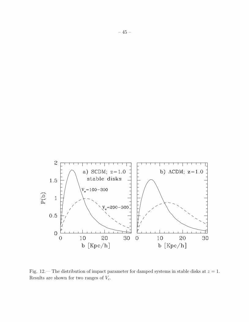
– 45 –

Fig. 12.— The distribution of impact parameter for damped systems in stable disks at z = 1.

Results are shown for two ranges of Vc.

– 46 –

Fig. 13.— Rotation curves for disk galaxies with central bulges (cf. Figure 2). The disk

and the bulge are assumed to have the same mass, 2.5× 1010h−1M⊙. The circular velocities

induced by the disk, the bulge and the dark matter are shown by long-dashed, dotted and

short-dashed lines, respectively. The total circular velocity is shown by the solid line. In

the top panel, the disk is assumed to have twice as much specific angular momentum as the

dark matter, while in the bottom panel the two specific angular momenta are assumed to be

the same. The central cusps in these rotation curves reflect our unrealistic assumption of a

point-mass bulge.

– 47 –

Fig. 14.— Disk scalelength, Rd, and disk rotation velocity, Vc(3Rd), in a model where the

mass of the central bulge (Mb) is equal to that of the disk (Md), as functions of the total

stellar mass fraction, md + mb. Results are shown in units of the values when Mb is set

to zero, We have assumed λ = 0.05 and c = 10. The solid curves show the results for

jd = md + mb, while the dashed curves show those for jd = md. The two dotted lines give a

rough indication of the scatter in the observed TF relation.