
Relativistic pseudopotential calculations for electronic excited states
Upload
khangminh22Category
view
0download
0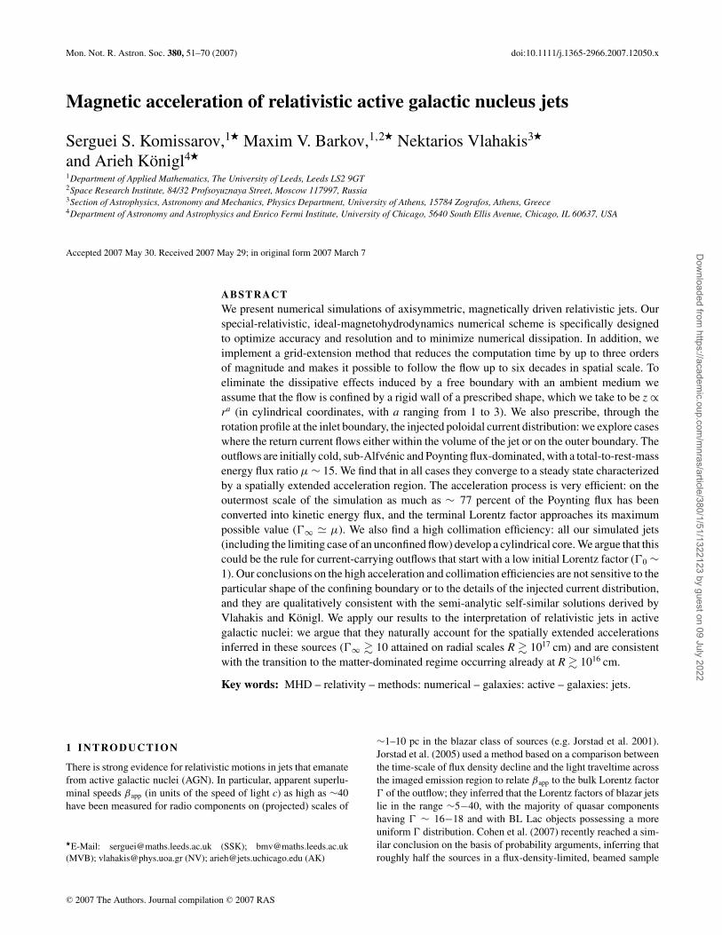
Mon. Not. R. Astron. Soc. 380, 51–70 (2007) doi:10.1111/j.1365-2966.2007.12050.x
Magnetic acceleration of relativistic active galactic nucleus jets
Serguei S. Komissarov,1� Maxim V. Barkov,1,2� Nektarios Vlahakis3�
and Arieh Konigl4�1Department of Applied Mathematics, The University of Leeds, Leeds LS2 9GT2Space Research Institute, 84/32 Profsoyuznaya Street, Moscow 117997, Russia3Section of Astrophysics, Astronomy and Mechanics, Physics Department, University of Athens, 15784 Zografos, Athens, Greece4Department of Astronomy and Astrophysics and Enrico Fermi Institute, University of Chicago, 5640 South Ellis Avenue, Chicago, IL 60637, USA
Accepted 2007 May 30. Received 2007 May 29; in original form 2007 March 7
ABSTRACTWe present numerical simulations of axisymmetric, magnetically driven relativistic jets. Ourspecial-relativistic, ideal-magnetohydrodynamics numerical scheme is specifically designedto optimize accuracy and resolution and to minimize numerical dissipation. In addition, weimplement a grid-extension method that reduces the computation time by up to three ordersof magnitude and makes it possible to follow the flow up to six decades in spatial scale. Toeliminate the dissipative effects induced by a free boundary with an ambient medium weassume that the flow is confined by a rigid wall of a prescribed shape, which we take to be z ∝ra (in cylindrical coordinates, with a ranging from 1 to 3). We also prescribe, through therotation profile at the inlet boundary, the injected poloidal current distribution: we explore caseswhere the return current flows either within the volume of the jet or on the outer boundary. Theoutflows are initially cold, sub-Alfvenic and Poynting flux-dominated, with a total-to-rest-massenergy flux ratio µ ∼ 15. We find that in all cases they converge to a steady state characterizedby a spatially extended acceleration region. The acceleration process is very efficient: on theoutermost scale of the simulation as much as ∼ 77 percent of the Poynting flux has beenconverted into kinetic energy flux, and the terminal Lorentz factor approaches its maximumpossible value (�∞ � µ). We also find a high collimation efficiency: all our simulated jets(including the limiting case of an unconfined flow) develop a cylindrical core. We argue that thiscould be the rule for current-carrying outflows that start with a low initial Lorentz factor (�0 ∼1). Our conclusions on the high acceleration and collimation efficiencies are not sensitive to theparticular shape of the confining boundary or to the details of the injected current distribution,and they are qualitatively consistent with the semi-analytic self-similar solutions derived byVlahakis and Konigl. We apply our results to the interpretation of relativistic jets in activegalactic nuclei: we argue that they naturally account for the spatially extended accelerationsinferred in these sources (�∞ � 10 attained on radial scales R � 1017 cm) and are consistentwith the transition to the matter-dominated regime occurring already at R � 1016 cm.
Key words: MHD – relativity – methods: numerical – galaxies: active – galaxies: jets.
1 I N T RO D U C T I O N
There is strong evidence for relativistic motions in jets that emanatefrom active galactic nuclei (AGN). In particular, apparent superlu-minal speeds βapp (in units of the speed of light c) as high as ∼40have been measured for radio components on (projected) scales of
�E-Mail: [email protected] (SSK); [email protected](MVB); [email protected] (NV); [email protected] (AK)
∼1–10 pc in the blazar class of sources (e.g. Jorstad et al. 2001).Jorstad et al. (2005) used a method based on a comparison betweenthe time-scale of flux density decline and the light traveltime acrossthe imaged emission region to relate βapp to the bulk Lorentz factor� of the outflow; they inferred that the Lorentz factors of blazar jetslie in the range ∼5−40, with the majority of quasar componentshaving � ∼ 16−18 and with BL Lac objects possessing a moreuniform � distribution. Cohen et al. (2007) recently reached a sim-ilar conclusion on the basis of probability arguments, inferring thatroughly half the sources in a flux-density-limited, beamed sample
C© 2007 The Authors. Journal compilation C© 2007 RAS
Dow
nloaded from https://academ
ic.oup.com/m
nras/article/380/1/51/1322123 by guest on 09 July 2022
52 S. S. Komissarov et al.
have a value of � close to the measured βapp. They further deducedthat the maximum Lorentz factor in their sample of 119 AGN jetsis ∼32, close to the value of ∼40 inferred for the jets observed byJorstad et al. (2001, 2005).
The presence of relativistic bulk motions in blazar jets has beenindependently indicated by measurements of rapid variations in thetotal and polarized fluxes (e.g. Hartman et al. 2001; Bach et al. 2006;Rebillot et al. 2006; Villata et al. 2006). There is also evidence thatthe relativistic speeds persist to large scales. For example, apparentsuperluminal component motions have been measured in the 3C120 jet out to projected distances from the source of at least 150 pc(Walker et al. 2001), and it has been argued that the spectral proper-ties of the heads of extended (up to several hundred kiloparsecs) jetscan be explained in the context of a relativistic flow that is deceler-ated to subrelativistic speeds at the termination shock that advancesinto the ambient medium (Georganopoulos & Kazanas 2003).
The main source of power of AGN jets is the rotational energy ofthe central supermassive black hole (e.g. Lovelace 1976; Blandford& Znajek 1977) and/or its accretion disc (e.g. Blandford 1976). Thenaturally occurring low-mass density and hence high magnetiza-tion of black hole magnetospheres suggests that the relativistic jetsoriginate directly from the black hole ergosphere, whereas the discsurface launches a slower, possibly non-relativistic wind that sur-rounds and confines the highly relativistic flow. This picture findssupport in recent numerical simulations (e.g McKinney & Gammie2004; De Villiers et al. 2005). However, this issue is far from settledand one cannot rule out the inner part of accretion disc as a base ofa relativistic outflow (e.g. Vlahakis & Konigl 2004). The theory ofrelativistic, magnetically driven jets from black holes (and neutronstars) predicts highly magnetized flows, with the Poynting flux dom-inating the total energy output. At the jet emission site this energyhas to be transferred to particles. This transfer may have the form ofmagnetic dissipation (e.g. Blandford 2002; Lyutikov & Blandford2003) but the still commonly held view is that the Poynting energy isfirst converted into bulk kinetic energy and only subsequently chan-nelled into radiation through shocks and other dissipative waves(e.g. Blandford & Rees 1974; Begelman, Blandford & Rees 1984).The jet radiative efficiency is still one of the key debatable issues inthe theory of Poynting-dominated outflows. In principle, slow mag-netic dissipation in an expanding jet may also facilitate the gradualconversion of Poynting flux into bulk kinetic energy (Drenkhahn &Spruit 2002).
When the inertia of the plasma is negligibly small its dynam-ics is well described by the approximation of force-free electrody-namics (or magnetodynamics; e.g. Komissarov 2002; Komissarov,Barkov & Lyutikov 2007). The equations of magnetodynamics aremuch simpler than those of magnetohydrodynamics (MHD), whichis what prompted their application to the study of the magnetic ac-celeration of relativistic jets (e.g. Blandford 1976, 2002; Narayan,McKinney & Farmer 2007). The solutions of these equations de-scribe trans-Alfvenic flows whose drift velocity approaches thespeed of light at infinity, the location of the fast critical point inthese models. However, within this framework it is impossible toaccount for the conversion of Poynting flux into plasma kinetic en-ergy and to study the issue of the acceleration efficiency.
The next simplest approximation that can be used to address theissue of Poynting-to-kinetic energy conversion is ideal MHD. Inthis case one can obtain exact semi-analytic solutions, although, be-cause of the complexity of the problem, this can only be done whenthe system possesses a high degree of symmetry. This approachwas pioneered by Blandford & Payne (1982), who constructednon-relativistic semi-analytic solutions for steady-state, cold, self-
similar (in the spherical radial coordinate) disc outflows. These so-lutions were generalized to the (special) relativistic MHD (RMHD)regime by Li, Chiueh & Begelman (1992) and Contopoulos (1994).They were further investigated by Vlahakis & Konigl (2003a,b),who also considered the effect of thermal forces during the earlyphases of the acceleration.1 Solutions with similar properties werederived in Beskin & Nokhrina (2006) by linearizing about a force-free solution for a paraboloidal field geometry.
A key property of the relativistic solutions derived in the afore-mentioned studies is the extended nature of the acceleration region:the bulk of the (poloidal) acceleration is effected by magnetic pres-sure gradients (associated with the azimuthal magnetic field compo-nent) and takes place beyond the classical fast-magnetosonic point(a singular point of the Bernoulli equation). Vlahakis & Konigl(2003a) interpreted this behaviour (which was dubbed the ‘mag-netic nozzle’ effect by Li et al. 1992; see also Camenzind 1989)in terms of the distinction between the classical and the modifiedfast-magnetosonic surfaces (e.g. Bogovalov 1997). They pointed outthat the latter surface, which is the locus of the fast-magnetosonicsingular points of the combined Bernoulli and trans-field (or Grad–Shafranov) equations, is the true causality surface (or ‘event hori-zon’) for the propagation of fast waves when the shape of the fieldlines is obtained from the solution of the trans-field equation (withthe classical surface playing this role only when the shape of the fluxsurfaces is pre-determined). They argued that, in this case, the accel-eration continues all the way to (and possibly even past) the modifiedfast-magnetosonic surface, which can lie well beyond the classicalone.2 Another general property of the cold MHD solutions is that, inthe current-carrying regime (where the poloidal components of thecurrent density and the magnetic field are antiparallel) they collimate(asymptotically) to cylinders. Furthermore, the asymptotic Lorentzfactor corresponds to a rough equipartition between the Poyntingand kinetic energy fluxes.
The continuation of the acceleration process beyond the classi-cal fast-magnetosonic surface is evidently a general characteristicof steady-state MHD solutions that applies also to non-relativisticjets (e.g. Vlahakis et al. 2000). This behaviour should, however, bemore clearly discerned in observations of relativistic flows, wherethe proper speed �β can increase by a large factor between theclassical and the modified singular surfaces. In contrast, the mag-netic acceleration of non-relativistic flows is almost complete at theclassical fast point. This striking difference has a very simple ori-gin. For non-relativistic flows the criticality condition at the classicalfast-magnetosonic point implies equipartition between the magneticenergy and the kinetic energy of poloidal motion. The kinetic en-ergy can therefore increase by at most a factor of 2 beyond thispoint. However, relativistic flows remain magnetically dominatedat the fast-magnetosonic point, which means that there is an am-ple remaining supply of magnetic energy that can be used for flowacceleration downstream of this point (e.g. Komissarov 2004).
In the case of AGN there have indeed been indications from agrowing body of data that the associated relativistic jets undergo
1 Vlahakis & Konigl (2003a) focused on flows whose initial poloidal velocitycomponent is sub-Alfvenic, corresponding to the poloidal magnetic fieldcomponent dominating the azimuthal field component at the top of the disc,whereas Vlahakis & Konigl (2003b) discussed the super-Alfvenic case inwhich the azimuthal component is dominant at the base of the flow. In thispaper we only consider outflows of the first type.2 In the radially self-similar solutions presented in Vlahakis & Konigl(2003a), the modified fast-magnetosonic surface formally lies at an infinitedistance from the origin.
C© 2007 The Authors. Journal compilation C© 2007 RAS, MNRAS 380, 51–70
Dow
nloaded from https://academ
ic.oup.com/m
nras/article/380/1/51/1322123 by guest on 09 July 2022
Magnetic acceleration of AGN jets 53
the bulk of their acceleration on scales that are of the order of thoseprobed by very long baseline radio interferometry. In one line ofreasoning, the absence of bulk-Comptonization spectral signaturesin blazars has been used to infer that jet Lorentz factors �10 areonly attained on scales � 1017 cm (Sikora et al. 2005). There havealso been explicit inferences of component acceleration based onradio proper motion and X-ray emission measurements for the jetsin the quasars 3C 345 (Unwin et al. 1997) and 3C 279 (Piner et al.2003). Extended acceleration in the 3C 345 jet has been indepen-dently indicated by the higher apparent speeds of jet componentslocated further away from the nucleus (Lobanov & Roland 2005)and by the observed luminosity variations of the moving compo-nents (Lobanov & Zensus 1999). Similar effects in other blazars(e.g. Homan et al. 2001) suggest that parsec-scale acceleration torelativistic speeds may be a common feature of AGN jets. Vlahakis& Konigl (2004) argued that these observations are most naturallyinterpreted in terms of magnetic driving and employed self-similarrelativistic jet solutions to generate model fits to the 3C 345 data insupport of this conclusion.
While the semi-analytic solutions have been useful in indicatingbasic properties of the magnetic acceleration process and in pro-viding valuable clues to the interpretation of the observational data,more general solutions are needed to confirm these results and togain a fuller understanding of the generation of relativistic jets inAGN. In particular, numerical simulations are needed to find outwhether the self-similar model captures the essential properties ofoutflows that obey realistic boundary conditions and that are notrequired to be in a steady state. Among the questions that such sim-ulations could answer are: (1) Do disc outflows in fact approach asteady state, and, if they do, is that state stable? (2) Is the accelerationindeed generally extended, and to what extent does the asymptoticstate of the self-similar solutions approximate the far-field behaviourof more realistic outflows? (3) Do any new traits emerge when therestrictions imposed by the self-similarity assumption are removed?Of particular interest is the question of the ability of the magneticdriving mechanism to accelerate outflows to high Lorentz factorswith high efficiency over astrophysically relevant distance scales.Another important question is whether highly relativistic flows canbe strongly collimated by purely magnetic stresses. There have beenlingering doubts over these issues in the literature (see Section 5.1),and although they have already received tentative answers, a fullnumerical study could help to settle them once and for all.
Although there have already been several reported simulationsof the formation of jets in black hole accretion flows using rela-tivistic (in fact, general relativistic) MHD codes, so far they haveprovided only partial answers to the above questions. The exist-ing calculations indicate that magnetic acceleration indeed operatesover several decades in radius and can accelerate jets to relativisticspeeds. However, the extended nature of the acceleration typicallyresults in the bulk Lorentz factor reaching only a small fraction of itspotential asymptotic value by the time the simulation is terminated.For example, in the longest jet simulated to date, which extendedto ∼104 times the gravitational radius rg of the central black hole(McKinney 2006), the Lorentz factor on the largest computed scalewas ∼10, which is just ∼ 10−2 to 10−3 of the estimated asymptoticvalue. This impressive simulation deals with an extremely complexsystem of which the jet is only one component, the other being theblack hole, the accretion disc, the disc corona, the low-speed ‘walljet’ and their surroundings. Ultimately, this is the kind of simulationone wants to carry out in order to fully understand the dynamics ofAGN outflows. However, they are also very challenging from thecomputational point of view. One major concern is that, in view of
the extended nature of its acceleration, the jet is particularly vulner-able to numerical diffusion and dissipation. These numerical effectsmay partly explain why the quantity �∞ in the above-cited paper,which is the same as our µ (equation 15) and should be a field lineconstant, in fact decreases by about one order of magnitude alonga mid-level field line in the simulated jet (see fig. 7 in McKinney2006).
In this paper we address the above questions through numericalsimulations specifically designed for investigating the key aspects ofideal MHD acceleration of relativistic jets. In the first place, we usea numerical scheme based on a linear Riemann solver (Komissarov1999) that does not need a large artificial diffusion for numericalstability. This distinguishes it from most other schemes for RMHD,including those that are based on HLL, KT and similar flux prescrip-tions (e.g. Koide, Shibata & Kudoh 1999; Del Zanna, Bucciantini &Londrillo 2003; Gammie, McKinney & Toth 2003; Duez et al. 2005;Shibata & Sekuguchi 2005; Anderson et al. 2006a; Anninos, Fragile& Salmonson 2006; Anton et al. 2006). Simple one-dimensionaltests suggest that this should lead to a noticeably greater accuracyin two-dimensional problems that involve stationary flows that arealigned with the computational grid (Komissarov 2006). Secondly,instead of studying jet propagation through some ambient medium,we consider the case of a flow in a funnel with solid walls. Thisallows us to avoid the errors that would otherwise be caused by nu-merical mass diffusion and dissipation at the interface. Finally, weemploy elliptical (or spherical) coordinates adapted to the chosenparaboloidal (or conical) shape of the funnel. This allows us to havethe jet well resolved everywhere (using a fixed number of grid pointsacross the funnel) and to benefit from the close alignment of the flowwith the computational grid. These careful measures in conjunctionwith a grid-extension method enable us, for the first time, to trackthe acceleration and collimation processes to their completion.
We describe the basic equations in Section 2 and the numericalcalculations in Section 3. The simulation results are presented inSection 4 and discussed in Section 5. We summarize in Section 6.
2 BA S I C E QUAT I O N S
Since most of the acceleration takes place far away from the source,we assume that the space–time is flat. Moreover, the flow is describedin an inertial frame at rest relative to the source. In this case we canwrite the system of ideal RMHD as follows. The continuity equation(
1
c
)∂t (
√−gρut ) + ∂i (√−gρui ) = 0, (1)
where ρ is the rest-mass density of matter, uν is its 4-velocity, andg is the determinant of the metric tensor; the energy–momentumequations(
1
c
)∂t
(√−gT tν
) + ∂i
(√−gT iν
) =√−g
2∂ν(gαβ )T αβ, (2)
where Tκν is the total stress–energy–momentum tensor; the induc-tion equation(
1
c
)∂t (Bi ) + ei jk∂ j (Ek) = 0, (3)
where ei jk = √γ εi jk is the Levi–Civita tensor of the absolute space
(ε123 = 1 for right-handed systems and ε123 = −1 for left-handedones) and γ is the determinant of the spatial part of the metric tensor(γ ij = gij); the solenoidal condition
∂i (√
γ Bi ) = 0. (4)
C© 2007 The Authors. Journal compilation C© 2007 RAS, MNRAS 380, 51–70
Dow
nloaded from https://academ
ic.oup.com/m
nras/article/380/1/51/1322123 by guest on 09 July 2022

54 S. S. Komissarov et al.
The total stress–energy–momentum tensor, Tκν , is a sum of thestress–energy momentum tensor of matter
T κν(m) = wuκuν
c2 + pgκν, (5)
where p is the thermodynamic pressure and w is the enthalpy perunit volume, and the stress–energy momentum tensor of the elec-tromagnetic field
T κν(e) = 1
4π
[Fκα Fν
α − 1
4
(Fαβ Fαβ
)gκν
], (6)
where Fνκ is the Maxwell tensor of the electromagnetic field. Theelectric and magnetic fields are defined as measured by an observerstationary relative to the spatial grid, which gives
Bi = 1
2ei jk Fjk (7)
and
Ei = Fit . (8)
In the limit of ideal MHD
Ei = − ei jkvj Bk
c, (9)
where vi = ui/ut is the usual 3-velocity of the plasma.We use an isentropic equation of state
p = Qρs, (10)
where Q = constant and s = 4/3. Since we are interested in themagnetic acceleration of cold flows, we make Q very small, so thegas pressure is never a dynamical factor. This relation enables us toexclude the energy equation from the integrated system. However,the momentum equation remains intact, including the non-linearadvection term. Therefore, if the conditions for shock formationwere to arise, our calculation would capture that shock.3
2.1 Field line constants
The poloidal magnetic field is fully described by the azimuthal com-ponent of the vector potential,
Bi = 1√γ
εi jφ ∂Aφ
∂x j. (11)
For axisymmetric solutions Aφ = �/2π, where �(xi), the so-called magnetic flux function, is the total magnetic flux enclosed bythe circle xi= constant (xi being the coordinates of the meridionalplane). Stationary and axisymmetric ideal MHD flows have fivequantities that propagate unchanged along the magnetic field linesand thus are functions of � alone. These are k, the rest-mass energyflux per unit magnetic flux; �, the angular velocity of magnetic fieldlines; l, the total angular momentum flux per unit rest-mass energyflux; µ, the total energy flux per unit rest-mass energy flux and Q,the entropy per particle. For cold flows (Q = 0, w = ρc2) we have
k = ρup
Bp, (12)
3 Since entropy is fixed the compression of our shocks would be the same asfor continuous compression waves. This gives a higher jump in density forthe same jump in pressure than in a proper dissipative shock. Fortunately,we do not need to contend with this issue in practice as shocks do not formin our simulations.
� = vφ
r− vp
r
B φ
Bp, (13)
l = − I
2πkc+ ruφ (14)
and
µ = � (1 + σ ) , (15)
where up = �vp is the magnitude of the poloidal component of the4-velocity, Bp is the magnitude of the poloidal component of themagnetic field, r is the cylindrical radius,
I = c
2r B φ (16)
is the total electric current flowing through a loop of radius r, σ isthe ratio of the Poynting flux to the matter (kinetic plus rest-mass)energy flux, and
�σ = − �I
2πkc3(17)
is the Poynting flux per unit rest-mass energy flux. (Here and inthe rest of the paper we use a hat symbol over vector indices toindicate their components in a normalized coordinate basis.) Fromequation (15) it follows that the Lorentz factor � cannot exceed µ.
3 N U M E R I C A L S I M U L AT I O N S
To maintain a firm control over the jet’s confinement and to pre-vent complications related to numerical diffusion of the dense non-relativistic plasma from the jet’s surroundings, we study outflowsthat propagate inside a solid funnel of a prescribed shape.4 Specifi-cally, we consider axisymmetric paraboloidal funnels
z ∝ ra,
where z and r are the cylindrical coordinates of the funnel wall.This suggests the utilization of a system of coordinates in whichthe funnel wall is a coordinate surface. For a conical jet (a = 1) weuse spherical coordinates, whereas for jets with a > 1 we employelliptical coordinates {ξ , η, φ}, where
ξ = r z−1/a (18)
and
η2 = r 2
a+ z2 (19)
(see Appendix A for details).5
We use a Godunov-type numerical code based on the schemedescribed in Komissarov (1999). To reduce numerical diffusion we
4 In real astrophysical systems, the shape of the boundary is determinedby the spatial distribution of the pressure or the density of the confiningambient medium (e.g. Blandford & Rees 1974; Konigl 1982; Komissarov1994). The effective ambient pressure distributions implied by the adoptedfunnel shapes are considered in Section 5.2.5 The equations are dimensionalized in the following manner. The unit oflength, L, is such that ηi = 1 L, where the subscript i refers to the inletboundary. The unit of time is T = L/c. The unit of mass is M = L3B2
0/4πc2,where B0 is the dimensional magnitude of the η component of magnetic fieldat the inlet (so the dimensionless magnitude of B η at the inlet is
√4π). In
applications, L is the length-scale of the launch region (e.g. the radius of theevent horizon if the jet originates in a black hole), T is the light crossing timeof that region and B0 is the typical strength of the poloidal magnetic field atthe origin.
C© 2007 The Authors. Journal compilation C© 2007 RAS, MNRAS 380, 51–70
Dow
nloaded from https://academ
ic.oup.com/m
nras/article/380/1/51/1322123 by guest on 09 July 2022
Magnetic acceleration of AGN jets 55
applied parabolic reconstruction instead of the linear one of the origi-nal code. Our procedure, in brief, was to calculate minmod-averagedfirst and second derivatives and use the first three terms of theTaylor expansion for spatial reconstruction. This simple procedurehas resulted in a noticeable improvement in the solution accuracyeven though the new scheme is still not third-order accurate becauseof the non-uniformity of the grid.
The grid is uniform in the ξ direction (the polar angle directionwhen we use spherical coordinates), where in most runs it has atotal of 60 cells. To check the convergence, some runs were repeatedwith a doubled resolution. The cells are elongated in the η direction(the radial direction when we use spherical coordinates), reflectingthe elongation of the funnel. For very elongated cells we observednumerical instability, so we imposed an upper limit of 40 on thelength/width ratio.
To speed up the simulations, we implemented a sectioning ofthe computational grid as described in Komissarov & Lyubarsky(2004). In each section, which is shaped as a ring, the numericalsolution is advanced using a time-step based on the local Courantcondition. It is twice as large as the time-step of the adjacent innerring and twice as small as the time-step of the adjacent outer ring.This approach is particularly effective for conical flows but less sofor highly collimated, almost cylindrical configurations.
3.1 Boundary conditions
3.1.1 Inlet boundary
We treat the inlet boundary, ηi = 1, as a surface of a perfectlyconducting rotator and consider two rotation laws,
� = �0 (20)
and
� = �0
[1 − 3
(ξ
ξj
)2
+ 2
(ξ
ξj
)3]
, (21)
where ξ j marks the jet boundary. The angular velocity profile isdirectly related to the distribution of the return electric current inthe jet (see equation 28 below). In fact, the current is driven bythe electric field associated with the rotating poloidal field, andcharge conservation requires the circuit to eventually close. In thecase of constant � the return current flows over the jet boundary.For the rotation law (21) it is distributed over the jet body as avolume current, the current changing sign at ξ � ξ j/2. Thus, wecover the two generic types of electric current distribution. Thesolid-body rotation law provides a very good description of thebehaviour of magnetic field lines that thread the horizon of a blackhole. This choice is therefore entirely appropriate for the black holetheory of relativistic AGN jets. The differential rotation law is moresuitable to the accretion disc theory, although it admittedly does notcorrespond to a realistic velocity field (which is hard to model giventhe limitations of our numerical technique).
The condition of perfect conductivity allows us to fix the az-imuthal component of the electric field and the η component of themagnetic field:
Eφ = 0, B η = B0 at η = ηi . (22)
From the first of these conditions we derive
vξ = vη
B ηB ξ (23)
and (using equation 13)
vφ = r� + vη
B ηB φ . (24)
We have also experimented with non-uniform distributions of themagnetic field, in particular with B η decreasing with ξ . The resultswere not significantly different as the field distribution downstreamof the inlet underwent a rapid rearrangement that restored the trans-verse force balance.
On the assumption of a cold (i.e. zero thermal energy) jet, theflow at the inlet boundary is necessarily super-slow-magnetosonic.This means that both the density and the radial component of thevelocity can be prescribed some fixed values:
ρ = ρ0, vη = vp0 .
In the simulations we used vp0 = 0.5 c, which was a choice ofconvenience. On one hand, this value is sufficiently small to insurethat the flow at η = 1 is sub-Alfvenic and hence that the Alfven andfast-magnetosonic critical surfaces are located downstream of theinlet boundary. On the other hand, it is large enough to promote arapid settlement to a steady state (keeping in mind that the speedof a steady-state flow remains constant along the symmetry axis).Because of the sub-Alfvenic nature of the inlet flow, we cannot fixthe other components of the magnetic field and the velocity – theyare to be found as part of the global solution. Following the standardapproach we extrapolate B φ and B ξ from the domain into the inletboundary cells. We then compute vφ and vξ from equations (23) and(24).
In the case of differential rotation the magnitude of the angularvelocity is chosen in such a way that the Alfven surface of the jetis near the jet origin, its closest point being located at a distance of∼1.5 times the initial jet radius from the inlet surface. In the caseof solid-body rotation the Alfven surface almost coincides with thelight cylinder, whose radius rlc ≡ c/� is only 50 per cent larger thanthe initial jet radius.
The inlet density is chosen so that all jets have very similar val-ues of µ and σ . In particular, for the models with uniform � wehave µmax � 18, and for the models with non-uniform � we haveµmax � 12.
3.1.2 Other boundaries
The computational domain is always chosen to be long enoughfor the jet to be super-fast-magnetosonic when it approaches theoutlet boundary η = η0. This justifies the use of radiative boundaryconditions at this boundary (i.e. we determine the state variables ofthe boundary cells via extrapolation of the domain solution).
At the polar axis, ξ = 0, we impose symmetry boundary condi-tions for the dependent variables that are expected to pass throughzero there,
f (−ξ ) = − f (ξ ).
These variables include B ξ , B φ , u ξ and uφ . For other variables weimpose a ‘zero second derivative’ condition,
∂2 f /∂ξ 2 = 0,
which means that we use linear interpolation to calculate the valuesof these variables in the boundary cells.
We do this in order to improve the numerical representation ofa narrow core that develops in all cases as a result of the magnetichoop stress. Within this core the gradients in the ξ direction are verylarge and the usual zero-gradient condition, f (−ξ ) = f (ξ ), results
C© 2007 The Authors. Journal compilation C© 2007 RAS, MNRAS 380, 51–70
Dow
nloaded from https://academ
ic.oup.com/m
nras/article/380/1/51/1322123 by guest on 09 July 2022
56 S. S. Komissarov et al.
in increased numerical diffusion in this region. We have checkedthat this has a noticeable effect only on the axial region and that theglobal solution does not depend on which of these two conditionsis used.
At the wall boundary, ξ = ξ j, we use a reflection condition,
f (ξj + �ξ ) = − f (ξj − �ξ ),
for B ξ and u ξ and a zero-gradient condition for all other variables.
3.2 Initial set-up
The initial configuration corresponds to a non-rotating, purelypoloidal magnetic field with approximately constant magnetic pres-sure across the funnel. The plasma density within the funnel is set toa small value so that the outflow generated at the inlet boundary caneasily sweep it away. In order to speed this process up the η compo-nent of velocity inside the funnel is set equal to 0.7 c, whereas theξ component is set equal to zero.
3.3 Grid extensions
The inner rings of the grid, where the grid cells are small and so isthe time-step, are the computationally most intensive regions of thesimulation domain. If we kept computing these inner rings duringthe whole run then we would not be able to advance very far from thejet origin. Fortunately, the trans-sonic nature of the jet flow allowsus to cease computations in the inner region once the solution theresettles to a steady state. To be more precise, we cut the funnel alongthe ξ -coordinate surfaces into overlapping sectors with the intentionof computing only within one sector at any given time, starting withthe sector closest to the inlet boundary. Once the solution in the‘active’ sector settles to a steady state we switch to the subsequentsector, located further away from the inlet. During the switch thesolution in the outermost cells of the active sector is copied into thecorresponding inner boundary cells of the subsequent sector. Duringthe computation within the latter sector these inner boundary cellsare not updated. Surely, this procedure is justified only when the flowin a given sector cannot communicate with the flow in the precedingsector through hyperbolic waves, and thus we need to ensure thatthe Mach cone of the fast-magnetosonic waves points outward atthe sector interfaces. This condition can be written as
(�vη)4 − (�vη)2
(b2
4πw/c2+ c2
s
1 − c2s /c2
)
+ c2s
1 − c2s /c2
(B η)2
4πw/c2
(1 − r 2
r 2lc
)> 0, (25)
where c2s = spc2/w (see equation 10) and b = (B2 − E2)1/2 is the
magnetic field magnitude in the fluid frame (see Appendix B fordetails). In the cold limit this reduces to
vη >
[1 −
(vξ
c
)2
−(
vφ
c
)2]1/2
cf, (26)
where cf = b/(4πρ + b2/c2)1/2 is the isotropic fast speed in the fluidframe. Thus, the jet has to be superfast in the η direction at the sectorinterfaces. In Figs 1–3 the location of the surface where vη = cf isshown by a thick solid line: to the right-hand side of this line vη > cf.One can see that the transition to the superfast regime occurs wellinside the first sector. (Note that when vη > cf the inequality 26 issatisfied.)
In these simulations we normally used four or five sectors, witheach additional sector being 10 times longer than the preceding
one. This technique has enabled us to reduce the computationaltime by up to three orders of magnitude, depending on the funnelgeometry. Although the grid extension can in principle be continuedindefinitely, there are other factors that limit how far along the jetone can advance in practice. First, once the paraboloidal jets becomehighly collimated the required number of grid cells along the jet axisincreases, and each successive sector becomes more expensive thanthe previous one. Secondly, computational errors due to numericaldiffusion gradually accumulate in the downstream region of the flowand the solution becomes progressively less accurate (see Fig. 4).
4 R E S U LT S
Models A, B, C and D have geometrical power indices a = 1, 3/2, 2and 3, respectively. Further classification is based on the rotationlaw: models A1–D1 have non-uniform rotation, whereas modelsA2–D2 have uniform rotation.
Models with different power indices but the same rotation lawshow remarkably similar properties. Thus, it is sufficient to showonly one of them in greater detail. For this purpose we selectedmodels C1, C2 and A2.
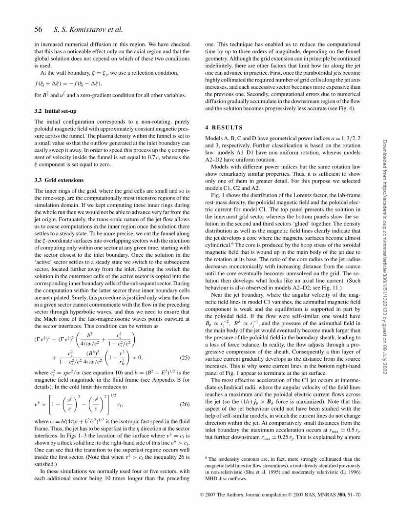
Fig. 1 shows the distribution of the Lorentz factor, the lab-framerest-mass density, the poloidal magnetic field and the poloidal elec-tric current for model C1. The top panel presents the solution inthe innermost grid sector whereas the bottom panels show the so-lution in the second and third sectors ‘glued’ together. The densitydistribution as well as the magnetic field lines clearly indicate thatthe jet develops a core where the magnetic surfaces become almostcylindrical.6 The core is produced by the hoop stress of the toroidalmagnetic field that is wound up in the main body of the jet due tothe rotation at its base. The ratio of the core radius to the jet radiusdecreases monotonically with increasing distance from the sourceuntil the core eventually becomes unresolved on the grid. The so-lution then develops what looks like an axial line current. (Suchbehaviour is also observed in models A2–D2; see Fig. 11.)
Near the jet boundary, where the angular velocity of the mag-netic field lines in model C1 vanishes, the azimuthal magnetic fieldcomponent is weak and the equilibrium is supported in part bythe poloidal field. If the flow were self-similar, one would haveBp ∝ r−2
j , B φ ∝ r−1j , and the pressure of the azimuthal field in
the main body of the jet would eventually become much larger thanthe pressure of the poloidal field in the boundary sheath, leading toa loss of force balance. In reality, the flow adjusts through a pro-gressive compression of the sheath. Consequently a thin layer ofsurface current gradually develops as the distance from the sourceincreases. This is why some current lines in the bottom right-handpanel of Fig. 1 appear to terminate at the jet surface.
The most effective acceleration of the C1 jet occurs at interme-diate cylindrical radii, where the angular velocity of the field linesreaches a maximum and the poloidal electric current flows acrossthe jet (so the (1/c) jp × Bφ force is maximized). Note that thisaspect of the jet behaviour could not have been studied with thehelp of self-similar models, in which the current lines do not changedirection within the jet. At comparatively small distances from theinlet boundary the maximum acceleration occurs at rmax � 0.5 rj,but further downstream rmax � 0.25 rj. This is explained by a more
6 The isodensity contours are, in fact, more strongly collimated than themagnetic field lines (or flow streamlines), a trait already identified previouslyin non-relativistic (Shu et al. 1995) and moderately relativistic (Li 1996)MHD disc outflows.
C© 2007 The Authors. Journal compilation C© 2007 RAS, MNRAS 380, 51–70
Dow
nloaded from https://academ
ic.oup.com/m
nras/article/380/1/51/1322123 by guest on 09 July 2022
Magnetic acceleration of AGN jets 57
Figure 1. Model C1. Left-hand panels show log10 �ρ (colour), where �ρ is the jet density as measured in the laboratory frame, and magnetic field lines.Right-hand panels show the Lorentz factor (colour) and the current lines. The thick solid line in the top-left-hand panel denotes the surface where the flowbecomes superfast in the η direction. The top panels show the solution for the first grid sector, whereas the bottom panels show the combined solution for thesecond and third grid sectors.
effective collimation in the inner region of the jet than at the jetboundary (see discussion following equation 29 in Section 5.1).
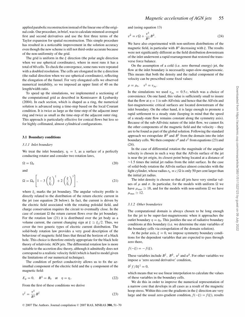
A careful inspection of the velocity field in the lower right-handpanel of Fig. 1 reveals an additional region of effective accelerationnear the jet axis for z � 103. This acceleration, however, is unphys-ical as it is caused by numerical diffusion/dissipation in the corethat results from large gradients of the flow variables that developthere. The gradual growth of errors in this region is clearly seen inFig. 4, which shows the flow constants as functions of � at vari-ous distances from the source. Beyond z = 104 the errors becomeunacceptably large and this makes further continuation of the so-lution via grid extension meaningless. We note in this connectionthat, even in the absence of exact analytic solutions, the existence offlow constants makes the jet problem a very useful one for testingRMHD codes and assessing their performance.
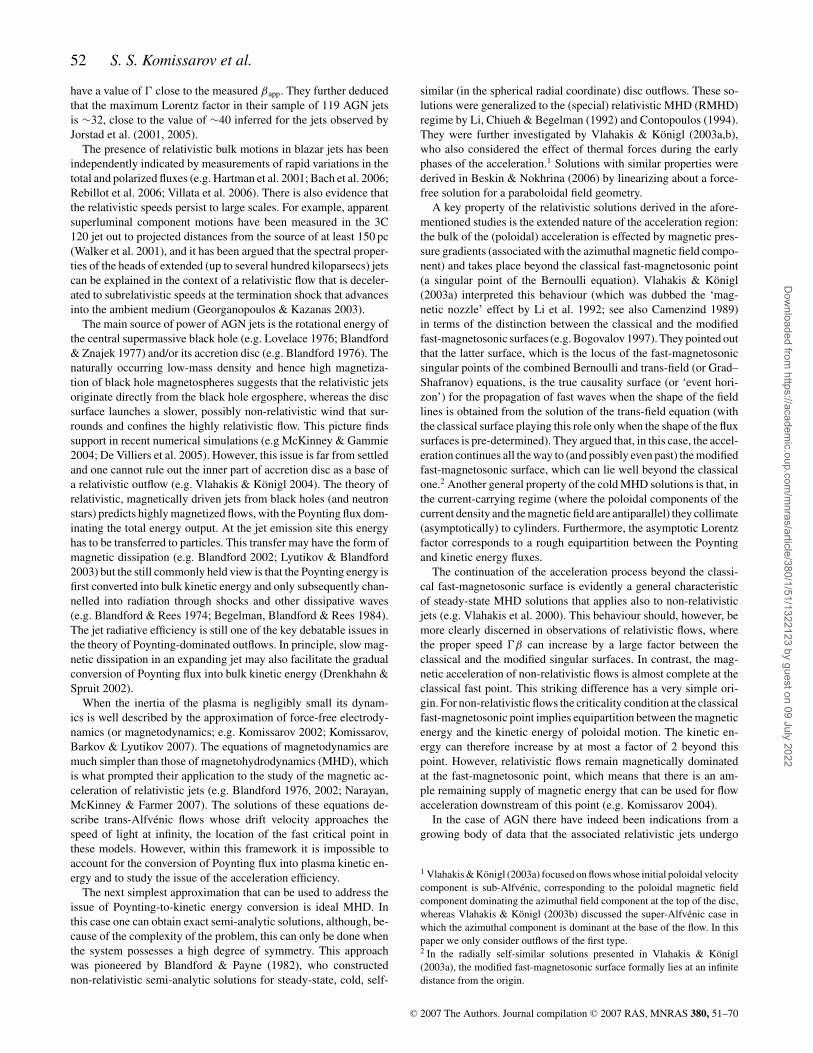
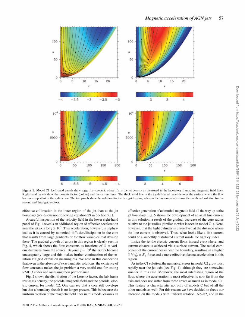
Fig. 2 shows the distribution of the Lorentz factor, the lab-framerest-mass density, the poloidal magnetic field and the poloidal elec-tric current for model C2. One can see that a core still developsbut that a boundary sheath is no longer present. This is because theuniform rotation of the magnetic field lines in this model ensures an
effective generation of azimuthal magnetic field all the way up to thejet boundary. Fig. 5 shows the development of an axial line currentin this solution, a result of the gradual decrease of the core radiusrelative to the jet radius (similar to what is seen in model C1). Note,however, that the light cylinder is unresolved at the distance wherethe line current is observed. Thus, what looks like a line currentcould be a smoothly distributed current inside the light cylinder.
Inside the jet the electric current flows inward everywhere, andcurrent closure is achieved via a surface current. The radial com-ponent of the current peaks near the boundary, resulting in a higher(1/c) jp × Bφ force and a more effective plasma acceleration in thisregion.
As in the C1 solution, the numerical errors in model C2 grow mostrapidly near the jet axis (see Fig. 4), although they are somewhatsmaller in this case. Moreover, the most interesting region of theflow, where the acceleration is most effective, is now far from theaxis and does not suffer from these errors as much as in model C1.This feature is characteristic not only of models C but of all theother models as well. For this reason we have decided to focus ourattention on the models with uniform rotation, A2–D2, and in the
C© 2007 The Authors. Journal compilation C© 2007 RAS, MNRAS 380, 51–70
Dow
nloaded from https://academ
ic.oup.com/m
nras/article/380/1/51/1322123 by guest on 09 July 2022
58 S. S. Komissarov et al.
Figure 2. Same as Fig. 1, but for Model C2.
rest of this section we present results mainly for these solutions.This choice is further motivated by the fact that models with a non-uniform rotation do not seem to exhibit any significant differenceswith respect to the uniform-rotation models besides those that wehave already described.
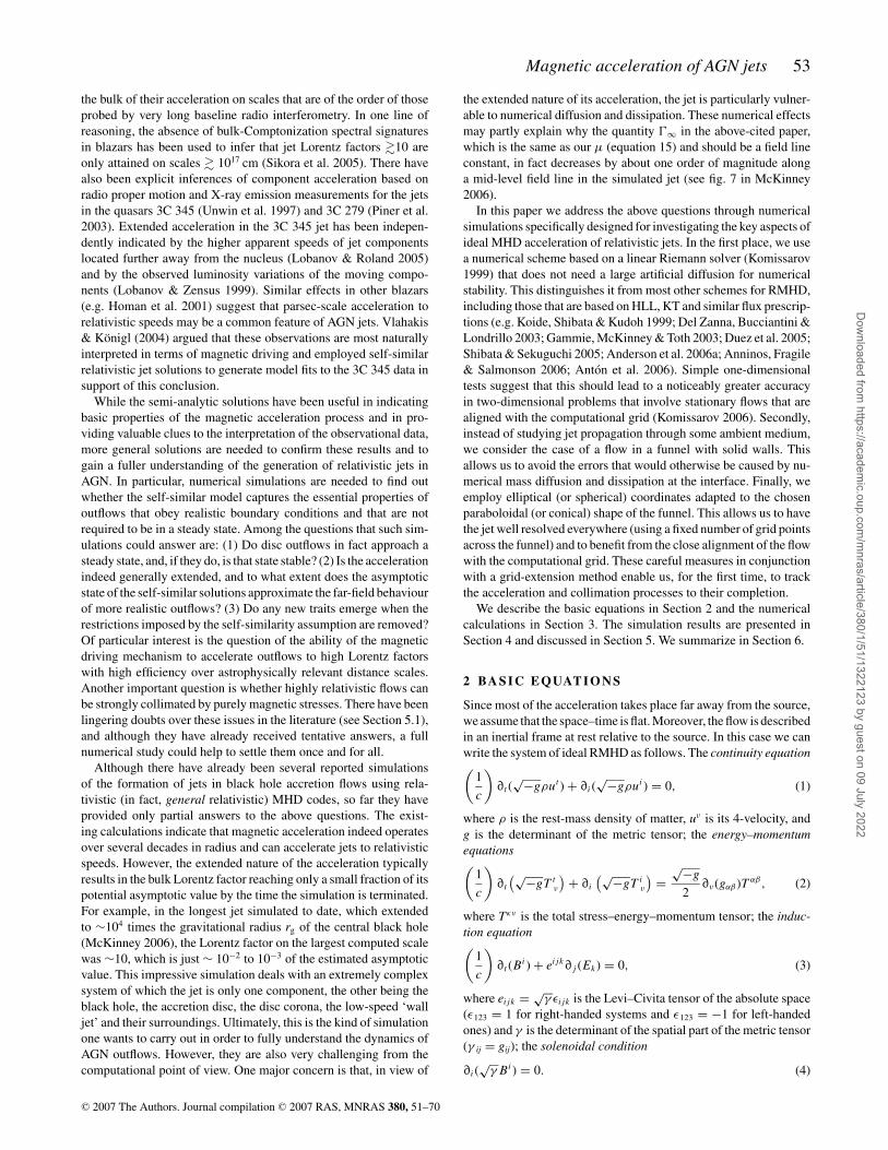
Given the results of previous analytical and numerical studies,which suggested poor self-collimation of relativistic magnetizedflows (see references in Section 5.1), one could have expected themagnetic flux surfaces to almost mirror the imposed shape of the jetboundary. However, our results indicate that the outflows collimatesignificantly faster, and that this property is manifested not only byjets with paraboloidal boundaries but also by the ones that are con-fined by a conical wall (see Fig. 3). Fig. 6 shows the magnetic fluxsurfaces and the coordinate surfaces ξ = constant for models A2and C2. In both cases the magnetic flux surfaces clearly do not di-verge as fast as the coordinate surfaces. This effect is further demon-strated by Fig. 7, which shows the evolution of the magnetic fluxdistribution across these jets (as well as the jet of model C1) withdistance from the origin. It is seen that the magnetic flux becomesprogressively more concentrated towards the symmetry axis as theflow moves further downstream.
The left-hand and middle panels of Fig. 8 show the evolution ofµ, �σ and � along selected magnetic surfaces for models C1 and
C2. For model C1 this flux surface is in the middle part of the jet,where the flow accelerates most rapidly; it encloses approximatelyone-third of the total magnetic flux in the jet. For model C2 thissurface is near the jet boundary, enclosing ∼5/6 of the total mag-netic flux in the jet. One can see that µ remains very nearly constanton the surfaces, indicating that the flow has reached a steady stateand that the computational errors that we have described above arefairly small. The Lorentz factor at first grows linearly with cylin-drical radius but then enters an extended domain of logarithmicgrowth. The linear behaviour was previously found in the magnet-ically dominated regime of self-similar solutions (e.g. Vlahakis &Konigl 2003a), whereas the logarithmic behaviour was shown tocharacterize the acceleration in the asymptotic matter-dominatedzone (e.g. Begelman & Li 1994). The range of Lorentz factors inthe solutions derived in this paper is evidently too narrow to allowus to probe the linear growth regime, but we expect that this couldbe done in our forthcoming paper where we consider higher �∞flows.
The magnetization function σ eventually becomes less than 1,signalling a transition to the matter-dominated regime. The right-hand panel of Fig. 8 shows the evolution of µ, �σ and � alongthe magnetic flux surface of model A2 that again encloses ∼5/6of the total magnetic flux in the jet. This conical jet also exhibits
C© 2007 The Authors. Journal compilation C© 2007 RAS, MNRAS 380, 51–70
Dow
nloaded from https://academ
ic.oup.com/m
nras/article/380/1/51/1322123 by guest on 09 July 2022
Magnetic acceleration of AGN jets 59
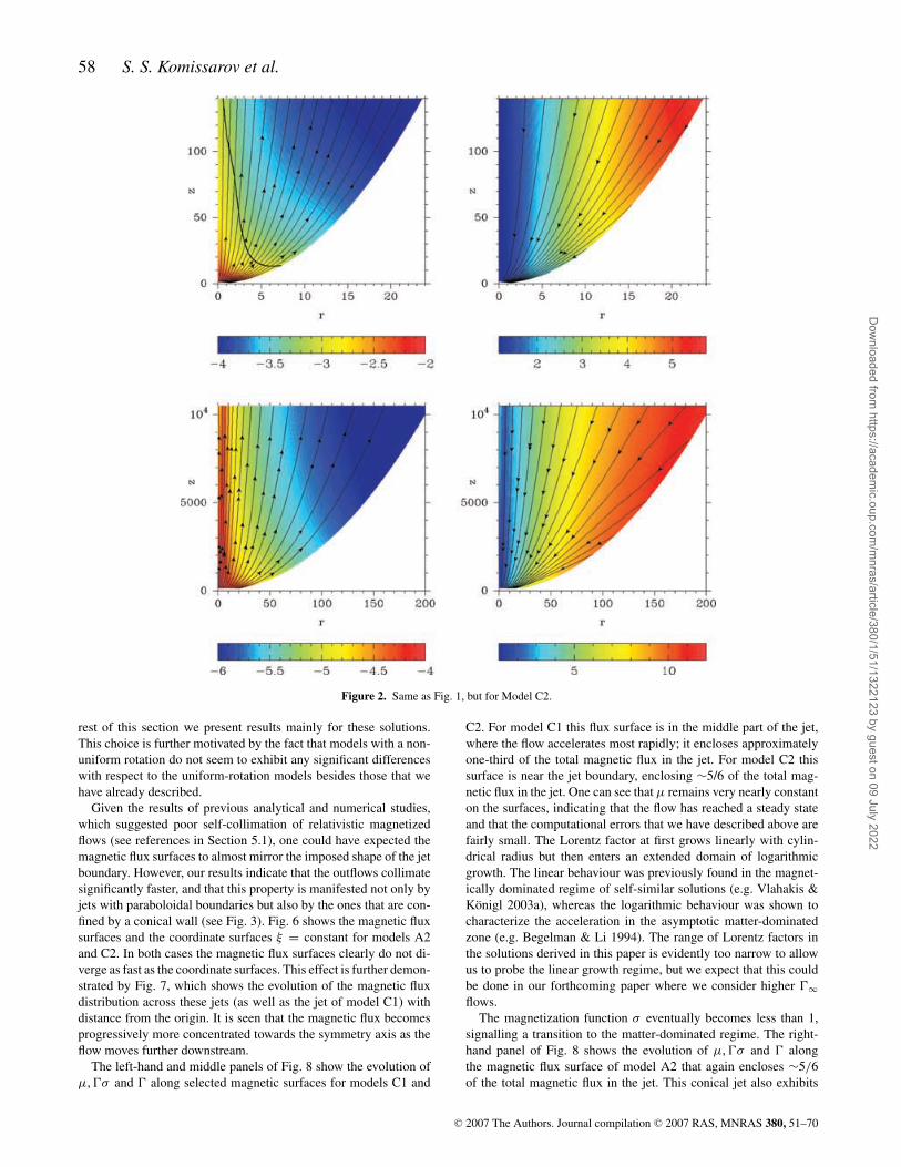
Figure 3. Same as Fig. 1, but for Model A2.
a very effective initial acceleration and a transition to a matter-dominated regime. In this case the growth of the Lorentz factorsaturates when it reaches � � 10, a value that corresponds to anacceleration efficiency �/µ of 77 per cent. Although the set-up of ourconical jet model most closely evokes the conical flow geometriesthat have in previous works produced very inefficient accelerations(see Section 5.1), the results displayed in Fig. 8 demonstrate thatthis case is not inherently different from the other ones. We discussthe reasons for this in Section 5.1. It is also worth noting that, whileour choice of flux surfaces in Fig. 8 was arbitrary, the behaviouralong these surfaces is fairly representative. To demonstrate this weshow in Fig. 9 the variation of the same parameters across the jetsat large distances from the inlet. One can see that the jets are matterdominated throughout the entire cross-section.
Fig. 10 compares the growth rates of � in models A2–D2. Thenumerical errors in these models are less restrictive than in modelsA1–D1 and make it possible to extend the simulations to largerspatial scales. Each of the plotted curves corresponds to the magneticsurface near the jet boundary that encloses ∼5/6 of the total magneticflux. The left-hand panel shows � as a function of the cylindricalradius normalized by the light cylinder radius. The most interestingfeature of this figure is the very similar growth of � for all models.In fact, up to r ∼ 10−50 rlc the curves for models A2, C2 and
D2 are almost identical. In model B2 the Lorentz factor increasessomewhat more slowly. Further inspection reveals another anomalyof model B2 – in contrast to the C2 and D2 cases, where the highestLorentz factor is found at the jet boundary, the fastest accelerationin the B2 solution occurs somewhat off the boundary. The reasonfor these anomalies is not clear but it may have something to dowith the curvature of magnetic field lines – given the lower value ofthe power-law index a, model B2 retains a higher curvature at largerradii than models C2 and D2. The reason why the model D curveis significantly shorter than the other is that the strong collimationof the jet rapidly renders the computation prohibitively expensivein this case.
Since more rapidly collimated jets reach the same cylindricalradius at a larger distance from the source, the similar growth ratesof the Lorentz factor with cylindrical radius imply a faster growthwith spherical radius for less collimated jets. This is exactly whatwe see in the right-hand panel of Fig. 10 – the conical jet of the A2model reaches a Lorentz factor of 10 at a distance from the originthat is almost 100 times shorter than that of the paraboloidal jet ofmodel C2.
Fig. 11 compares the magnitudes of the different magnetic fieldcomponents in models A2–C2 near the far end of the jet (η = 103).At this distance the jet radius is almost 103 larger than the light
C© 2007 The Authors. Journal compilation C© 2007 RAS, MNRAS 380, 51–70
Dow
nloaded from https://academ
ic.oup.com/m
nras/article/380/1/51/1322123 by guest on 09 July 2022
60 S. S. Komissarov et al.
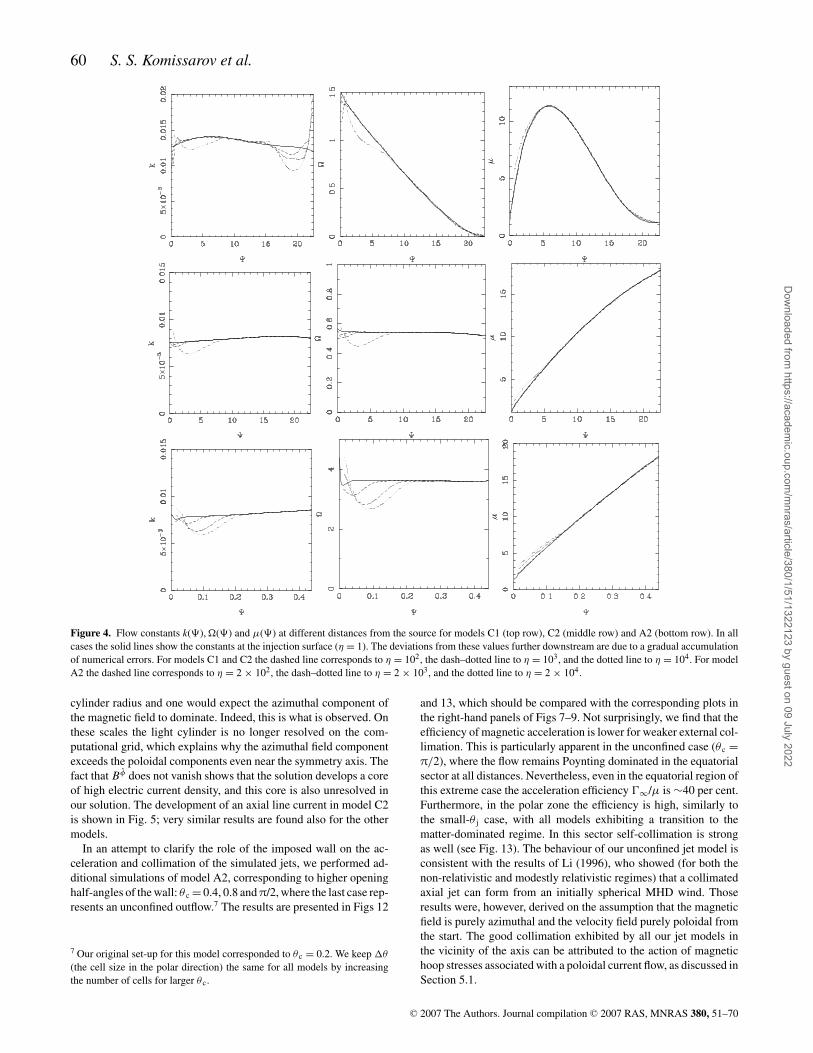
Figure 4. Flow constants k(�), �(�) and µ(�) at different distances from the source for models C1 (top row), C2 (middle row) and A2 (bottom row). In allcases the solid lines show the constants at the injection surface (η = 1). The deviations from these values further downstream are due to a gradual accumulationof numerical errors. For models C1 and C2 the dashed line corresponds to η = 102, the dash–dotted line to η = 103, and the dotted line to η = 104. For modelA2 the dashed line corresponds to η = 2 × 10², the dash–dotted line to η = 2 × 10³, and the dotted line to η = 2 × 10⁴.
cylinder radius and one would expect the azimuthal component ofthe magnetic field to dominate. Indeed, this is what is observed. Onthese scales the light cylinder is no longer resolved on the com-putational grid, which explains why the azimuthal field componentexceeds the poloidal components even near the symmetry axis. Thefact that B φ does not vanish shows that the solution develops a coreof high electric current density, and this core is also unresolved inour solution. The development of an axial line current in model C2is shown in Fig. 5; very similar results are found also for the othermodels.
In an attempt to clarify the role of the imposed wall on the ac-celeration and collimation of the simulated jets, we performed ad-ditional simulations of model A2, corresponding to higher openinghalf-angles of the wall: θ c = 0.4, 0.8 and π/2, where the last case rep-resents an unconfined outflow.7 The results are presented in Figs 12
7 Our original set-up for this model corresponded to θ c = 0.2. We keep �θ
(the cell size in the polar direction) the same for all models by increasingthe number of cells for larger θ c.
and 13, which should be compared with the corresponding plots inthe right-hand panels of Figs 7–9. Not surprisingly, we find that theefficiency of magnetic acceleration is lower for weaker external col-limation. This is particularly apparent in the unconfined case (θ c =π/2), where the flow remains Poynting dominated in the equatorialsector at all distances. Nevertheless, even in the equatorial region ofthis extreme case the acceleration efficiency �∞/µ is ∼40 per cent.Furthermore, in the polar zone the efficiency is high, similarly tothe small-θ j case, with all models exhibiting a transition to thematter-dominated regime. In this sector self-collimation is strongas well (see Fig. 13). The behaviour of our unconfined jet model isconsistent with the results of Li (1996), who showed (for both thenon-relativistic and modestly relativistic regimes) that a collimatedaxial jet can form from an initially spherical MHD wind. Thoseresults were, however, derived on the assumption that the magneticfield is purely azimuthal and the velocity field purely poloidal fromthe start. The good collimation exhibited by all our jet models inthe vicinity of the axis can be attributed to the action of magnetichoop stresses associated with a poloidal current flow, as discussed inSection 5.1.
C© 2007 The Authors. Journal compilation C© 2007 RAS, MNRAS 380, 51–70
Dow
nloaded from https://academ
ic.oup.com/m
nras/article/380/1/51/1322123 by guest on 09 July 2022

Magnetic acceleration of AGN jets 61
Figure 5. Development of the line current in model C2. The figure shows theazimuthal magnetic field at η = 200, 400, 800, 1600, 3200 and 6400 (frombottom to top). The solution at η = 6400 is plotted as squares.
5 D I S C U S S I O N
5.1 Theoretical aspects of the problem
Over the years there have been persistent doubts in the literature re-garding the ability of magnetic forces to accelerate flows to relativis-tic speeds. In particular, several published studies have concludedthat MHD acceleration of relativistic flows is inherently inefficient.This conclusion, however, is erroneous and can be attributed tothe adoption of a conical (split-monopole) flow geometry in thesestudies. For example, in the work of Michel (1969) a simplified con-ical geometry was used in which the full system of RMHD equa-tions was not satisfied, whereas the results of Beskin, Kuznetsova& Rafikov (1998) were based on a perturbative analysis around aquasi-conical flow. The conical flow geometry is unfavourable foracceleration for the following reason. Well outside the light cylinder,where r� vφ and v � c, equations (23) and (24) imply
r B φ = −1
c�Bpr 2. (27)
Figure 6. Poloidal magnetic field lines (solid) and ξ = constant coordinate lines (dashed) for models C2 (left-hand panel) and A2 (right-hand panel). In allmodels the magnetic field lines show faster collimation than the coordinate lines.
From this equation and equation (16) one finds that
I = −1
2�Bpr 2, (28)
where Bp is the magnitude of the poloidal magnetic field. If themagnetic surfaces are conical then Bp ∝ r−2, and thus the poloidalelectric current flows parallel to the magnetic field lines. In this casethe component of the Lorentz force along the poloidal magnetic fieldlines, (1/c) jp × Bφ , simply vanishes. More general treatments of theproblem, based on exact semi-analytic solutions for axisymmetric,highly magnetized, steady outflows under the assumption of radialself-similarity (Li et al. 1992; Vlahakis & Konigl 2003a,b, 2004),have demonstrated that magnetic acceleration in non-conical ge-ometries can be quite efficient, typically resulting in a rough asymp-totic equipartition between the Poynting and matter energy fluxes.A similar conclusion was reached on the basis of a perturbativeanalysis around a parabolic flow (Beskin & Nokhrina 2006). Theseresults have indicated that the correct paradigm should, in fact, bethat magnetic acceleration is generally a rather efficient mechanismfor producing relativistic flows.
In this paper we have for the first time verified the proposedparadigm by means of numerical simulations of highly magnetized,relativistic flows. We have focused on the parameter regime that ismost relevant to AGN jets. In a future paper (Komissarov et al., inpreparation) we will present additional simulations that will demon-strate that this paradigm also applies to flows with terminal Lorentzfactors that are as high as those inferred in gamma-ray burst sources.
One of the interesting outcomes of this study is the highly effectiveacceleration even in the case where the shape of the outer boundaryis conical. Although the acceleration efficiency in conical steadyflows is – as explained above – tiny, our results show that magneticsurfaces of conical jets are not conical but rather paraboloidal (seeFigs 6 and 7), so Bpr2 is not constant. Fig. 14 shows the evolutionof the function
S = πr 2 Bp
�= πr 2 Bp∫
Bp ·dS(29)
along a typical magnetic surface for models C2 and A2. It is seen thatin both cases S undergoes a significant decrease with distance fromthe source. In fact, this decrease is faster in the conical boundarymodel, which is reflected in the more rapid acceleration in this case(see Fig. 10). The direct relationship between the function S and theacceleration efficiency can be readily shown by combining equations
C© 2007 The Authors. Journal compilation C© 2007 RAS, MNRAS 380, 51–70
Dow
nloaded from https://academ
ic.oup.com/m
nras/article/380/1/51/1322123 by guest on 09 July 2022
62 S. S. Komissarov et al.
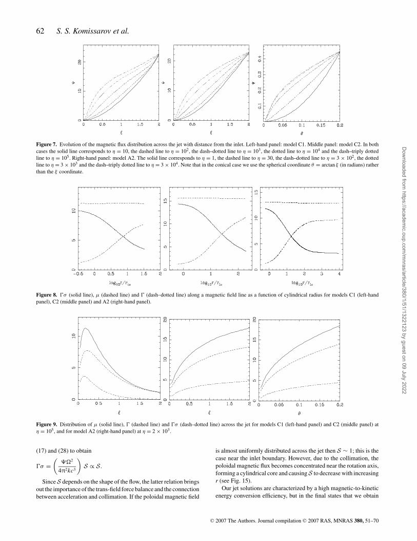
Figure 7. Evolution of the magnetic flux distribution across the jet with distance from the inlet. Left-hand panel: model C1. Middle panel: model C2. In bothcases the solid line corresponds to η = 10, the dashed line to η = 102, the dash–dotted line to η = 103, the dotted line to η = 104 and the dash–triply dottedline to η = 105. Right-hand panel: model A2. The solid line corresponds to η = 1, the dashed line to η = 30, the dash–dotted line to η = 3 × 10², the dottedline to η = 3 × 10³ and the dash–triply dotted line to η = 3 × 10⁴. Note that in the conical case we use the spherical coordinate θ = arctan ξ (in radians) ratherthan the ξ coordinate.
Figure 8. �σ (solid line), µ (dashed line) and � (dash–dotted line) along a magnetic field line as a function of cylindrical radius for models C1 (left-handpanel), C2 (middle panel) and A2 (right-hand panel).
Figure 9. Distribution of µ (solid line), � (dashed line) and �σ (dash–dotted line) across the jet for models C1 (left-hand panel) and C2 (middle panel) atη = 105, and for model A2 (right-hand panel) at η = 2 × 10³.
(17) and (28) to obtain
�σ =(
��2
4π2kc3
)S ∝ S.
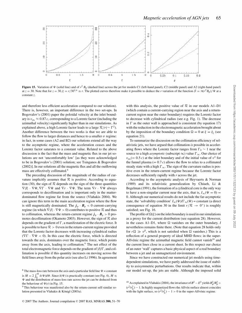
SinceS depends on the shape of the flow, the latter relation bringsout the importance of the trans-field force balance and the connectionbetween acceleration and collimation. If the poloidal magnetic field
is almost uniformly distributed across the jet then S ∼ 1; this is thecase near the inlet boundary. However, due to the collimation, thepoloidal magnetic flux becomes concentrated near the rotation axis,forming a cylindrical core and causingS to decrease with increasingr (see Fig. 15).
Our jet solutions are characterized by a high magnetic-to-kineticenergy conversion efficiency, but in the final states that we obtain
C© 2007 The Authors. Journal compilation C© 2007 RAS, MNRAS 380, 51–70
Dow
nloaded from https://academ
ic.oup.com/m
nras/article/380/1/51/1322123 by guest on 09 July 2022
Magnetic acceleration of AGN jets 63
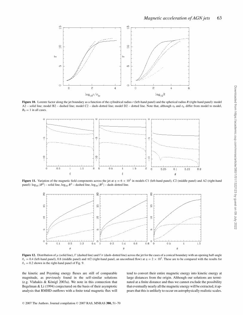
Figure 10. Lorentz factor along the jet boundary as a function of the cylindrical radius r (left-hand panel) and the spherical radius R (right-hand panel): modelA2 – solid line; model B2 – dashed line; model C2 – dash–dotted line; model D2 – dotted line. Note that, although r0 and rlc differ from model to model,R0 = 1 in all cases.
Figure 11. Variation of the magnetic field components across the jet at η = 6 × 10³ in models C1 (left-hand panel), C2 (middle panel) and A2 (right-handpanel): log10 |Bφ | – solid line, log10 B η – dashed line, log10 |B ξ | – dash–dotted line.
Figure 12. Distribution of µ (solid line), � (dashed line) and �σ (dash–dotted line) across the jet for the cases of a conical boundary with an opening half-angleθ c = 0.4 (left-hand panel), 0.8 (middle panel) and π/2 (right-hand panel, an unconfined flow) at η = 2 × 10³. These are to be compared with the results forθ c = 0.2 shown in the right-hand panel of Fig. 9.
the kinetic and Poynting energy fluxes are still of comparablemagnitude, as previously found in the self-similar solutions(e.g. Vlahakis & Konigl 2003a). We note in this connection thatBegelman & Li (1994) conjectured on the basis of their asymptoticanalysis that RMHD outflows with a finite total magnetic flux will
tend to convert their entire magnetic energy into kinetic energy atlarge distances from the origin. Although our solutions are termi-nated at a finite distance and thus we cannot exclude the possibilitythat eventually nearly all the magnetic energy will be extracted, it ap-pears that this is unlikely to occur on astrophysically realistic scales.
C© 2007 The Authors. Journal compilation C© 2007 RAS, MNRAS 380, 51–70
Dow
nloaded from https://academ
ic.oup.com/m
nras/article/380/1/51/1322123 by guest on 09 July 2022
64 S. S. Komissarov et al.
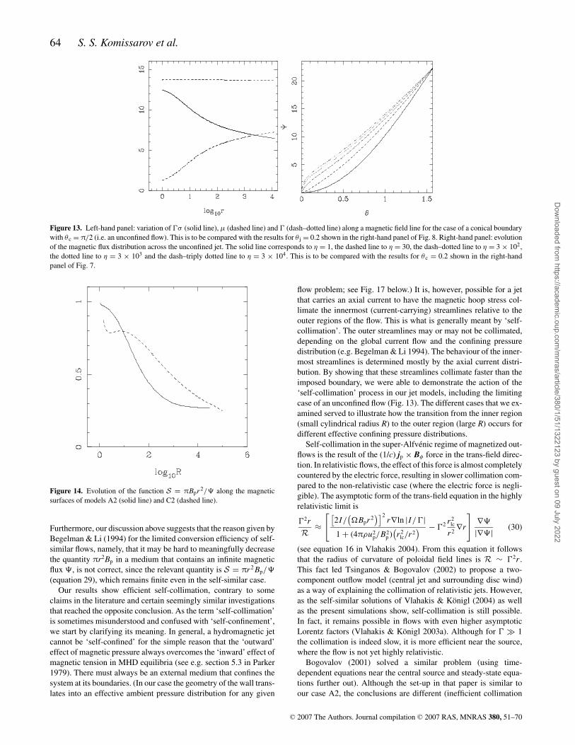
Figure 13. Left-hand panel: variation of �σ (solid line), µ (dashed line) and � (dash–dotted line) along a magnetic field line for the case of a conical boundarywith θ c = π/2 (i.e. an unconfined flow). This is to be compared with the results for θ j = 0.2 shown in the right-hand panel of Fig. 8. Right-hand panel: evolutionof the magnetic flux distribution across the unconfined jet. The solid line corresponds to η = 1, the dashed line to η = 30, the dash–dotted line to η = 3 × 10²,the dotted line to η = 3 × 10³ and the dash–triply dotted line to η = 3 × 10⁴. This is to be compared with the results for θ c = 0.2 shown in the right-handpanel of Fig. 7.
Figure 14. Evolution of the function S = πBpr2/� along the magneticsurfaces of models A2 (solid line) and C2 (dashed line).
Furthermore, our discussion above suggests that the reason given byBegelman & Li (1994) for the limited conversion efficiency of self-similar flows, namely, that it may be hard to meaningfully decreasethe quantity πr2Bp in a medium that contains an infinite magneticflux �, is not correct, since the relevant quantity is S = πr 2 Bp/�
(equation 29), which remains finite even in the self-similar case.Our results show efficient self-collimation, contrary to some
claims in the literature and certain seemingly similar investigationsthat reached the opposite conclusion. As the term ‘self-collimation’is sometimes misunderstood and confused with ‘self-confinement’,we start by clarifying its meaning. In general, a hydromagnetic jetcannot be ‘self-confined’ for the simple reason that the ‘outward’effect of magnetic pressure always overcomes the ‘inward’ effect ofmagnetic tension in MHD equilibria (see e.g. section 5.3 in Parker1979). There must always be an external medium that confines thesystem at its boundaries. (In our case the geometry of the wall trans-lates into an effective ambient pressure distribution for any given
flow problem; see Fig. 17 below.) It is, however, possible for a jetthat carries an axial current to have the magnetic hoop stress col-limate the innermost (current-carrying) streamlines relative to theouter regions of the flow. This is what is generally meant by ‘self-collimation’. The outer streamlines may or may not be collimated,depending on the global current flow and the confining pressuredistribution (e.g. Begelman & Li 1994). The behaviour of the inner-most streamlines is determined mostly by the axial current distri-bution. By showing that these streamlines collimate faster than theimposed boundary, we were able to demonstrate the action of the‘self-collimation’ process in our jet models, including the limitingcase of an unconfined flow (Fig. 13). The different cases that we ex-amined served to illustrate how the transition from the inner region(small cylindrical radius R) to the outer region (large R) occurs fordifferent effective confining pressure distributions.
Self-collimation in the super-Alfvenic regime of magnetized out-flows is the result of the (1/c) jp × Bφ force in the trans-field direc-tion. In relativistic flows, the effect of this force is almost completelycountered by the electric force, resulting in slower collimation com-pared to the non-relativistic case (where the electric force is negli-gible). The asymptotic form of the trans-field equation in the highlyrelativistic limit is
�2r
R ≈[[
2I/(�Bpr 2
)]2r∇ln |I/�|
1 + (4πρu2p/B2
p )(r 2
lc/r 2) − �2 r 2
lc
r 2∇r
]∇�
|∇�| (30)
(see equation 16 in Vlahakis 2004). From this equation it followsthat the radius of curvature of poloidal field lines is R ∼ �2r .This fact led Tsinganos & Bogovalov (2002) to propose a two-component outflow model (central jet and surrounding disc wind)as a way of explaining the collimation of relativistic jets. However,as the self-similar solutions of Vlahakis & Konigl (2004) as wellas the present simulations show, self-collimation is still possible.In fact, it remains possible in flows with even higher asymptoticLorentz factors (Vlahakis & Konigl 2003a). Although for � 1the collimation is indeed slow, it is more efficient near the source,where the flow is not yet highly relativistic.
Bogovalov (2001) solved a similar problem (using time-dependent equations near the central source and steady-state equa-tions further out). Although the set-up in that paper is similar toour case A2, the conclusions are different (inefficient collimation
C© 2007 The Authors. Journal compilation C© 2007 RAS, MNRAS 380, 51–70
Dow
nloaded from https://academ
ic.oup.com/m
nras/article/380/1/51/1322123 by guest on 09 July 2022
Magnetic acceleration of AGN jets 65
Figure 15. Variation of � (solid line) and of r2 Bp (dashed line) across the jet for models C1 (left-hand panel), C2 (middle panel) and A2 (right-hand panel)at z = 30. Note that for z = 30, ξ = r/301/a ∝ r. The plotted curves therefore make it possible to deduce the r variation of the function S = π(r2 Bp)/� at aconstant z.
and therefore less efficient acceleration compared to our solution).There is, however, an important difference in the two set-ups. InBogovalov’s (2001) paper the poloidal velocity at the inlet bound-ary is vp0 ≈ 0.87 c, corresponding to a Lorentz factor (including theazimuthal velocity) significantly higher than in our simulations. Asexplained above, a high Lorentz factor leads to a large R/r (∼ �2).Another difference between the two works is that we are able tofollow the flow to larger distances and hence to a smaller σ regime:in fact, in some cases (A2 and B2) our solutions extend all the wayto the asymptotic regime, where the acceleration ceases and theLorentz factor saturates to a constant value. Related to the abovediscussion is the fact that the mass and magnetic flux in our jet so-lutions are not ‘uncomfortably low’ [as they were acknowledgedto be in Bogovalov’s (2001) solution; see Tsinganos & Bogovalov(2002)]. In our solutions all the magnetic flux and all the outflowingmass are effectively collimated.8
The preceding discussion of the magnitude of the radius of cur-vature implicitly assumes that R is positive. According to equa-tion (30), the sign of R depends on the sign of the three quantities∇|I| · ∇�, ∇� · ∇� and ∇r · ∇�. The term ∇r · ∇� alwayscorresponds to decollimation and is important only in the matter-dominated flow regime far from the source (Vlahakis 2004). Wecan ignore this term in the main acceleration region where the flowis still magnetically dominated. The jp · Bp < 0 current-carryingregime (in which ∇|I| · ∇� > 0) contributes to positive R and thusto collimation, whereas the return-current regime jp · Bp > 0 pro-motes decollimation (Okamoto 2003). However, the sign of R alsodepends on the gradient of �, a manifestation of the electric force. Itis possible to haveR > 0 even in the return-current regime providedthat the Lorentz factor decreases with increasing cylindrical radius(∇� · ∇� < 0). In this case the electric force, which is directedtowards the axis, dominates over the magnetic force, which pointsaway from the axis, leading to collimation.9 The net effect of thetotal electromagnetic force depends on the gradient of |I|/�, and col-limation is possible if this quantity increases on moving across thefield lines away from the polar axis (see also Li 1996). In agreement
8 The mass-loss rate between the axis and a particular field line � = constant
is M = 2∫ �
0k(�)d�. Since k(�) is practically constant (see Fig. 4), M ∝
� and the distribution of mass-loss rate across the jet can be deduced fromthe behaviour of �(r) in Fig. 15.9 This behaviour was manifested also by the return-current self-similar so-lution presented in Vlahakis & Konigl (2003a).
with this analysis, the positive value of R in our models A1–D1(which contain a current-carrying region near the axis and a return-current region near the outer boundary) requires the Lorentz factorto decrease with cylindrical radius (see e.g. Fig. 1). The decreasein � as the outer wall is approached is consistent (by equation 17)with the reduction in the electromagnetic acceleration brought aboutby the imposition of the boundary condition � = 0 at ξ = ξ j (seeequation 21).
To summarize the discussion on the collimation efficiency of rel-ativistic jets, we have argued that collimation is possible in acceler-ating flows where the Lorentz factor ranges from �0 ∼ 1 near thesource to a high asymptotic (subscript ∞) value �∞. Our choice ofvp0 (= 0.5 c) at the inlet boundary and of the initial value of vη forthe funnel plasma (= 0.7 c) allows the flow to relax to a collimatedsteady state with a high �∞. The sign of the curvature radius is pos-itive even in the return-current regime because the Lorentz factordecreases sufficiently rapidly with r across the jet.
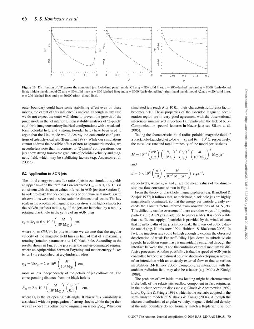
According to the asymptotic analysis of Heyvaerts & Norman(1989) and its relativistic generalization by Chiueh, Li &Begelman (1991), the formation of a cylindrical core is the only wayto have a non-singular current near the axis, that is, I∞(� = 0) =0. Although our numerical results do not include the far-asymptoticstate, the ‘solvability condition’ I∞(�)/�∞(�) = constant (a directconsequence of equation 30 in the limit r/R → 0+) is roughlysatisfied; see Fig. 16.
The profile of�(ξ ) on the inlet boundary is used in our simulationsas a proxy for the current distribution (see equation 28). However,in the cases A1–D1, where � vanishes on the outer boundary, Inevertheless remains finite there. (Note that equation 28 holds onlyfor r� vφ , which is not satisfied when � vanishes.) This is areflection of a general property of ideal MHD flows: in the super-Alfvenic regime the azimuthal magnetic field cannot vanish10 andthe current lines close in a current sheet. In this respect our choiceof an outer ‘wall’ captures a basic physical aspect of a real boundarybetween a jet and an unmagnetized environment.
Since we have constructed our numerical jet models using time-dependent simulations, we have partly addressed the issue of stabil-ity to axisymmetric perturbations. Our results indicate that, withinour model set-up, the jets are stable. Although the imposed solid
10 As explained in Vlahakis (2004), the invariance of B2 − E2 yields B2φ /B2
p >
(r2/r2lc) − 1. In highly magnetized flows the Alfven surface almost coincides
with the light surface, so (r2/r2lc) − 1 > 0 in the super-Alfvenic regime.
C© 2007 The Authors. Journal compilation C© 2007 RAS, MNRAS 380, 51–70
Dow
nloaded from https://academ
ic.oup.com/m
nras/article/380/1/51/1322123 by guest on 09 July 2022
66 S. S. Komissarov et al.
Figure 16. Distribution of I/� across the computed jets. Left-hand panel: model C1 at η = 80 (solid line), η = 800 (dashed line) and η = 8000 (dash–dottedline); middle panel: model C2 at η = 80 (solid line), η = 800 (dashed line) and η = 8000 (dash–dotted line); right-hand panel: model A2 at η = 20 (solid line),η = 200 (dashed line) and η = 20 000 (dash–dotted line).
outer boundary could have some stabilizing effect even on thesemodes, the extent of this influence is unclear, although in any casewe do not expect the outer wall alone to prevent the growth of thepinch mode in the jet interior. Linear stability analyses of ‘Z-pinch’equilibria (magnetostatic cylindrical configurations with a weak uni-form poloidal field and a strong toroidal field) have been used toargue that the kink mode would destroy the concentric configura-tions of astrophysical jets (Begelman 1998). While our simulationscannot address the possible effect of non-axisymmetric modes, wenevertheless note that, in contrast to ‘Z-pinch’ configurations, ourjets show strong transverse gradients of poloidal velocity and mag-netic field, which may be stabilizing factors (e.g. Anderson et al.2006b).
5.2 Application to AGN jets
The initial energy-to-mass flux ratio of jets in our simulations yieldsan upper limit on the terminal Lorentz factor �∞ = µ � 16. This isconsistent with the mean values inferred in AGN jets (see Section 1).In order to make further comparisons of our numerical models withobservations we need to select suitable dimensional scales. The keyscale in the problem of magnetic acceleration is the light cylinder (orthe Alfven surface) radius, rlc. If the jets are launched by a rapidlyrotating black hole in the centre of an AGN then
rlc � 4rg = 6 × 10¹³
(M
108 M�
)cm,
where rg ≡ GM/c2. In this estimate we assume that the angularvelocity of the magnetic field lines is half of that of a maximallyrotating (rotation parameter a � 1.0) black hole. According to theresults shown in Fig. 8, the jets enter the matter-dominated regime,where an equipartition between Poynting and matter energy fluxes(σ � 1) is established, at a cylindrical radius
req � 30 rlc � 2 × 10¹⁵
(M
108 M�
)cm,
more or less independently of the details of jet collimation. Thecorresponding distance from the black hole is
Req � 2 × 10¹⁶
(M
108 M�
)(�j
0.1
)−1
cm,
where �j is the jet opening half-angle. If blazar flux variability isassociated with the propagation of strong shocks within the jet thenwe can expect this behaviour to originate on scales �Req. When our
simulated jets reach R � 10 Req, their characteristic Lorentz factorbecomes ∼10. These properties of the extended magnetic accel-eration region are in very good agreement with the observationalinferences summarized in Section 1 (in particular, the lack of bulk-Comptonization spectral features in blazar jets; see Sikora et al.2005).
Taking the characteristic initial radius poloidal magnetic field ofa black hole-launched jet to be r0 = rg and B0 = 105 G, respectively,the mass-loss rate and total luminosity of the model jets scale as
M = 10−2
(k�
0.2
)(B0
105 G
)2 (r0
rg
)2 (M
108 M�
)2
M� yr−1
and
E = 6 × 1045
(µ
10
)(M
10−2 M� yr−1
)erg s−1,
respectively, where k, � and µ are the mean values of the dimen-sionless flow constants shown in Fig. 4.
From the theory of black hole magnetospheres (e.g. Blandford &Znajek 1977) it follows that, at their base, black hole jets are highlymagnetically dominated, so that the energy per particle greatly ex-ceeds the Lorentz factor inferred from observations of AGN jets.This difficulty can be overcome if there are other ways of injectingparticles into AGN jets in addition to pair cascades. It is conceivablethat a sufficient supply of particles is provided by the winds of starsthat lie in the paths of the jets as they make their way out of the galac-tic nuclei (e.g. Komissarov 1994; Hubbard & Blackman 2006). Infact, the injection rate could be high enough to explain the observeddeceleration of weak Fanaroff–Riley I jets down to subrelativisticspeeds. In addition some mass is unavoidably entrained through theinterface between the jet and the confining external medium via dif-fusive processes. Another possibility is that the speed of AGN jets iscontrolled by the dissipation at oblique shocks developing as a resultof an interaction with an unsteady external flow or due to variousinstabilities (McKinney 2006). Compton-drag interaction with theambient radiation field may also be a factor (e.g. Melia & Konigl1989).
The problem of low initial mass loading might be circumventedif the bulk of the relativistic outflow component in fact originatesin the nuclear accretion disc (see e.g. Ghosh & Abramowicz 1997;Livio, Ogilvie & Pringle 1999), which is the scenario adopted in thesemi-analytic models of Vlahakis & Konigl (2004). Although thechosen distributions of angular velocity, magnetic field and densityat the inlet boundary do not formally match a Keplerian disc, our
C© 2007 The Authors. Journal compilation C© 2007 RAS, MNRAS 380, 51–70
Dow
nloaded from https://academ
ic.oup.com/m
nras/article/380/1/51/1322123 by guest on 09 July 2022
Magnetic acceleration of AGN jets 67
solutions can be interpreted in the context of disc-driven outflows.Taking �K(r0) to be the Keplerian angular velocity at the referencedistance r0, we find that
rlc = 5 × 10¹⁴
(M
108 M�
)(r0
10 rg
)3/2 [�K(r0)
�
]cm
and that σ ≈ 1 is reached at a distance
Req � 1017
(rlc
5 × 1014 cm
)(�j
0.1
)−1
cm.
The mass-loss rate and jet power are
M = 10−2
(k�
0.2
)(B0
104 G
)2 (r0
10 rg
)2 (M
108 M�
)2
M� yr−1
and
E = 6 × 1045
(µ
10
)(M
10−2 M� yr−1
)erg s−1,
respectively. The striking differences in the velocity profile betweensimulated jets with solid-body rotation and with differential rotation(see Figs 1 and 2 for models C1 and C2, respectively) suggests(taking into account relativistic beaming effects) that it might bepossible to distinguish between jets launched directly from a blackhole and those that emanate from the surface of an accretion discin cases where the transverse structure of the jet can be resolved.One would, however, need to verify that these differences remainnoticeable for more realistic disc rotation laws and surface fielddistributions.
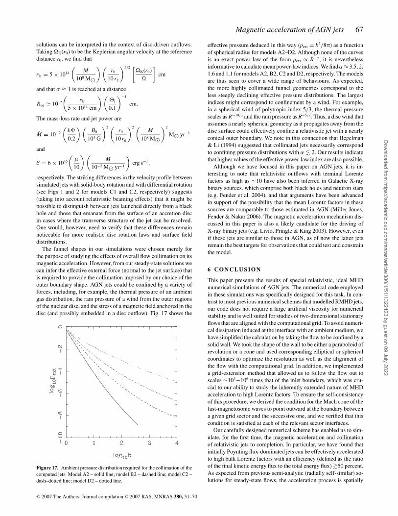
The funnel shapes in our simulations were chosen merely forthe purpose of studying the effects of overall flow collimation on itsmagnetic acceleration. However, from our steady-state solutions wecan infer the effective external force (normal to the jet surface) thatis required to provide the collimation imposed by our choice of theouter boundary shape. AGN jets could be confined by a variety offorces, including, for example, the thermal pressure of an ambientgas distribution, the ram pressure of a wind from the outer regionsof the nuclear disc, and the stress of a magnetic field anchored in thedisc (and possibly embedded in a disc outflow). Fig. 17 shows the
Figure 17. Ambient pressure distribution required for the collimation of thecomputed jets. Model A2 – solid line; model B2 – dashed line; model C2 –dash–dotted line; model D2 – dotted line.
effective pressure deduced in this way (pext = b2/8π) as a functionof spherical radius for models A2–D2. Although none of the curvesis an exact power law of the form pext ∝ R−α , it is neverthelessinformative to calculate mean power-law indices. We find α ≈ 3.5, 2,1.6 and 1.1 for models A2, B2, C2 and D2, respectively. The modelsare thus seen to cover a wide range of behaviours. As expected,the more highly collimated funnel geometries correspond to theless steeply declining effective pressure distributions. The largestindices might correspond to confinement by a wind. For example,in a spherical wind of polytropic index 5/3, the thermal pressurescales as R−10/3 and the ram pressure as R−5/2. Thus, a disc wind thatassumes a nearly spherical geometry as it propagates away from thedisc surface could effectively confine a relativistic jet with a nearlyconical outer boundary. We note in this connection that Begelman& Li (1994) suggested that collimated jets necessarily correspondto confining pressure distributions with α � 2. Our results indicatethat higher values of the effective power-law index are also possible.
Although we have focused in this paper on AGN jets, it is in-teresting to note that relativistic outflows with terminal Lorentzfactors as high as ∼10 have also been inferred in Galactic X-raybinary sources, which comprise both black holes and neutron stars(e.g. Fender et al. 2004), and that arguments have been advancedin support of the possibility that the mean Lorentz factors in thesesources are comparable to those estimated in AGN (Miller-Jones,Fender & Nakar 2006). The magnetic acceleration mechanism dis-cussed in this paper is also a likely candidate for the driving ofX-ray binary jets (e.g. Livio, Pringle & King 2003). However, evenif these jets are similar to those in AGN, as of now the latter jetsremain the best targets for observations that could test and constrainthe model.
6 C O N C L U S I O N
This paper presents the results of special relativistic, ideal MHDnumerical simulations of AGN jets. The numerical code employedin these simulations was specifically designed for this task. In con-trast to most previous numerical schemes that modelled RMHD jets,our code does not require a large artificial viscosity for numericalstability and is well suited for studies of two-dimensional stationaryflows that are aligned with the computational grid. To avoid numeri-cal dissipation induced at the interface with an ambient medium, wehave simplified the calculation by taking the flow to be confined by asolid wall. We took the shape of the wall to be either a paraboloid ofrevolution or a cone and used corresponding elliptical or sphericalcoordinates to optimize the resolution as well as the alignment ofthe flow with the computational grid. In addition, we implementeda grid-extension method that allowed us to follow the flow out toscales ∼104−106 times that of the inlet boundary, which was cru-cial to our ability to study the inherently extended nature of MHDacceleration to high Lorentz factors. To ensure the self-consistencyof this procedure, we derived the condition for the Mach cone of thefast-magnetosonic waves to point outward at the boundary betweena given grid sector and the successive one, and we verified that thiscondition is satisfied at each of the relevant sector interfaces.
Our carefully designed numerical scheme has enabled us to sim-ulate, for the first time, the magnetic acceleration and collimationof relativistic jets to completion. In particular, we have found thatinitially Poynting flux-dominated jets can be effectively acceleratedto high bulk Lorentz factors with an efficiency (defined as the ratioof the final kinetic energy flux to the total energy flux) �50 percent.As expected from previous semi-analytic (radially self-similar) so-lutions for steady-state flows, the acceleration process is spatially
C© 2007 The Authors. Journal compilation C© 2007 RAS, MNRAS 380, 51–70
Dow
nloaded from https://academ
ic.oup.com/m
nras/article/380/1/51/1322123 by guest on 09 July 2022

68 S. S. Komissarov et al.
extended. We have found that our simulated jets invariably settle to asteady state, which suggests (although we did not explore this issueexplicitly) that the resulting flow configurations are not inherentlyunstable (at least not to axisymmetric perturbations – although it isconceivable that the imposed rigid wall has a stabilizing influencein this regard – and excluding by design any effects of a direct in-teraction with an ambient medium). The properties of the derivedfinal configurations were found to be qualitatively very similar tothose of the self-similar AGN jet solutions of Vlahakis & Konigl(2004) and to not depend sensitively either on the imposed shapeof the outer boundary or on the distribution of the injected poloidalcurrent at the inlet boundary. (We explored boundaries with scal-ings, in cylindrical coordinates, ranging from z ∝ r to z ∝ r3, andcurrent distributions that closed either within the volume of the jetor on its outer boundary.)
We provided a physical explanation of the basic acceleration pro-cess and of the variations in the detailed behaviour among the dif-ferent flow configurations that we simulated. We argued that therobustness of the acceleration process can be attributed to the factthat the bulk of the outflow initially follows paraboloidal trajectories,including the case of a conical outer boundary. We highlighted theconnection between the collimation of the flow, which is manifestedin the curved streamlines, and the acceleration process. The colli-mation in the current-carrying regime is essentially due to magnetichoop stress associated with the azimuthal magnetic field componentBφ . The collimation induces a reduction in the magnitude of r2Bp
(where Bp is the poloidal field component) along the poloidal stream-lines, which corresponds to a decrease in the Poynting flux alongthe flow and therefore results in acceleration (driven by the gradientof the magnetic pressure associated with Bφ). Previous claims inthe literature that magnetic acceleration of relativistic flows is inef-ficient were all based on the assumption that the streamlines havea split-monopole geometry (or very nearly so), which is a singularcase in which by fiat r2Bp remains constant (or close to a constant)along the flow.
Our solutions also revealed that the collimation efficiency of rela-tivistic jets can be high if they are accelerated from an initial Lorentzfactor �0 ∼ 1. We argued that published results in the literature thatclaimed otherwise in fact had a significantly higher �0. Once theflow attains a high Lorentz factor the collimation process slows downon account of the increased inertia and of the growth of the electricforce, which almost completely balances the transverse magneticforce. Nevertheless, the current-carrying central region of our sim-ulated jets collimates much faster than the imposed boundaries andattains a cylindrical shape by the time the terminal Lorentz factor isattained, again in full agreement with the semi-analytic self-similarsolutions (which also assumed �0 ∼ 1). In simulated outflows wherethe current returns through the jet we found that the flow is effec-tively collimated also in the outer, return-current region (in this caseby the electric force, which dominates the transverse magnetic forcethat acts to decollimate the flow in this regime). The efficient electro-magnetic collimation in all of our computed jet models is evidentlythe reason why the presence of a rigid outer boundary does not in-duce recollimation shocks in the outflow even for the most rapidlyconverging wall shape (r ∝ z3).
In validating the basic features of the simplified semi-analyticsolutions, our numerical results go a long way towards establish-ing an ‘MHD acceleration and collimation paradigm’ for relativis-tic astrophysical jets. In this contribution we applied this modelto AGN jets, for which there is already significant observationalevidence of extended, �0.1 pc-scale acceleration (possibly contin-uing to ∼1−10 pc) to Lorentz factors �10. We demonstrated that,
for plausible physical parameters, our simulated jets can reproducethese observations (see also Vlahakis & Konigl 2004). We notedthat these results could potentially apply also to the jets observedin Galactic X-ray binary sources. In a future publication we willpresent simulation results for even higher initial magnetizations thatcould be used to model the ultrarelativistic jets in gamma-ray burstsources.
Future investigations will need to examine some of the complicat-ing factors left out of the present study. In particular, the simplifyingwall boundary condition will have to be replaced by the interactionof the outflow with its environment. Furthermore, the questions ofstability and energy dissipation will have to be addressed. In fact,given the potentially destructive role of the kink mode, fully three-dimensional relativistic simulations will ultimately need to be car-ried out. In addition, the response of the jet to non-steady conditionsat the source – a potential cause of observed variability – will be aninteresting topic for study.
AC K N OW L E D G M E N T S
We thank Mitch Begelman and Anatoly Spitkovsky for helpful com-ments and Jonathan McKinney for useful correspondence. We alsoacknowledge extensive suggestions by the referee. This researchwas funded by PPARC under the rolling grant ‘Theoretical As-trophysics in Leeds’ (SSK and MVB). NV acknowledges partialsupport by the European Social Fund and National Resources –(EPEAEK II) PYTHAGORAS. AK was partially supported by aNASA Theoretical Astrophysics Programme grant.
R E F E R E N C E S
Anderson M., Hirschmann E. W., Liebling S. L., Neilsen D., 2006a, Class.Quantum Gravity, 23, 6503
Anderson J. M., Li Z.-Y., Krasnopolsky R., Blandford R. D., 2006b, ApJ,653, L33
Anninos P., Fragile P. C., Salmonson J. D., 2005, ApJ, 635, 723Anton L., Zanotti O., Miralles J. A., Martı J. M., Ibanez J. M., Font J. A.,
Pons J. A., 2006, ApJ, 637, 296Bach U., Krichbaum T. P., Kraus A., Witzel A., Zensus J. A., 2006, A&A,
452, 83Begelman M. C., 1998, ApJ, 493, 291Begelman M. C., Li Z.-Y., 1994, ApJ, 326, 269Begelman M. C., Blandford R. D., Rees M. J., 1984, Rev. Mod. Phys., 56,
255Beskin V. S., Nokhrina E. E., 2006, MNRAS, 367, 375Beskin V. S., Kuznetsova I. V., Rafikov R. R., 1998, MNRAS, 299, 341Blandford R. D., 1976, MNRAS, 176, 465Blandford R. D., 2002, in Gilfanov M., Sunyeav R., Churazov E., eds, Light-
houses of the Universe. Springer-Verlag, Berlin, p. 381Blandford R. D., Payne D. G., 1982, MNRAS, 199, 883Blandford R. D., Rees M. J., 1974, MNRAS, 169, 395Blandford R. D., Znajek R. L., 1977, MNRAS, 179, 433Bogovalov S. V., 1997, A&A, 323, 634Bogovalov S. V., 2001, A&A, 371, 1155Camenzind M., 1989, in Belvedere G., ed., Accretion Disks and Magnetic
Fields in Astrophysics. Kluwer, Dordrecht, p. 129Chiueh T., Li Z.-Y., Begelman M. C., 1991, ApJ, 377, 462Cohen M. H., Lister M. L., Homan D. C., Kadler M., Kellermann K. I.,
Kovalev Y. Y., Vermeulen R. C., 2007, ApJ, 658, 232Contopoulos J., 1994, ApJ, 432, 508De Villiers J.-P., Hawley J. F., Krolik J. H., Hirose S., 2005, ApJ, 620, 878Del Zanna L., Bucciantini N., Londrillo P., 2003, A&A, 400, 397Drenkhahn G., Spruit H. C., 2002, A&A, 391, 1141Duez M. D., Liu Y. T., Shapiro S. L., Stephens B. C., 2005, Phys. Rev. D,
72, 024028
C© 2007 The Authors. Journal compilation C© 2007 RAS, MNRAS 380, 51–70
Dow
nloaded from https://academ
ic.oup.com/m
nras/article/380/1/51/1322123 by guest on 09 July 2022
Magnetic acceleration of AGN jets 69
Fender R., Wu K., Johnston H., Tzioumis T., Jonker P., Spencer R., van derKlis M., 2004, Nat, 427, 222
Gammie C. F., McKinney J. C., Toth G., 2003, ApJ, 589, 444Georganopoulos M., Kazanas D., 2003, ApJ, 589, L5Ghosh P., Abramowicz M. A., 1997, MNRAS, 292, 887Hartman R. C. et al., 2001, ApJ, 553, 683Heyvaerts J., Norman C., 1989, ApJ, 347, 1055Homan D. C., Ojha R., Wardle J. F. C., Roberts D. H., Aller M. F., Aller H.
D., Hughes P. A., 2001, ApJ, 549, 840Hubbard A., Blackman E. G., 2006, MNRAS, 371, 1717Jorstad S. G., Marscher A. P., Mattox J. R., Wehrle A. E., Bloom S. D.,
Yurchenko A. V., 2001, ApJS, 134, 181Jorstad S. G. et al., 2005, AJ, 130, 1418Koide S., Shibata K., Kudoh T., 1999, ApJ, 522, 727Komissarov S. S., 1994, MNRAS, 266, 649Komissarov S. S., 1999, MNRAS, 303, 343Komissarov S. S., 2002, MNRAS, 350, 1431Komissarov S. S., 2004, MNRAS, 350, 1431Komissarov S. S., 2006, in Hughes P. A., Bregman J. N., eds, AIP Conf. Proc.
Vol. 856, Relativistic Jets: The Common Physics of AGN, Microquasarsand Gamma Ray Bursts. Springer, Heidelberg, p. 129
Komissarov S. S., Lyubarsky Y. E., 2004, MNRAS, 349, 779Komissarov S. S., Barkov M., Lyutikov M., 2007, MNRAS, 374, 415Konigl A., 1982, ApJ, 261, 115Li Z.-Y., 1996, ApJ, 473, 873Li Z.-Y., Chiueh T., Begelman M. C., 1992, ApJ, 394, 459Livio M., Ogilvie G. I., Pringle J. E., 1999, ApJ, 512, 100Livio M., Pringle J. E., King A. R., 2003, ApJ, 593, 184Lobanov A. P., Roland J., 2005, A&A, 431, 831Lobanov A. P., Zensus J. A., 1999, ApJ, 521, 509Lovelace R. V. E., 1976, Nat, 262, 649Lyutikov M., Blandford R. D., 2003, online-only reference (astro-
ph/0312347)McKinney J. C., 2006, MNRAS, 368, 1561McKinney J. C., Gammie C. F., 2004, ApJ, 611, 977Melia F., Konigl A., 1989, ApJ, 340, 162Michel F. C., 1969, ApJ, 158, 727Miller-Jones J. C. A., Fender R. P., Nakar E., 2006, MNRAS, 367, 1432Narayan R., McKinney J. C., Farmer A. J., 2007, MNRAS, 375, 548Okamoto I., 2003, ApJ, 589, 671Parker E. N., 1979, Cosmical Magnetic Fields. Clarendon, OxfordPiner B. G., Unwin S. C., Wehrle A. E., Zook A. C., Urry C. M., Gilmore
D. M., 2003, ApJ, 588, 716Rebillot P. F. et al., 2006, ApJ, 641, 740Shibata M., Sekuguchi Y. I., 2005, Phys. Rev. D, 72, 044014Shu F. H., Najita J., Ostriker E. C., Shang H., 1995, ApJ, 455, L155Sikora M., Begelman M. C., Madejski G. M., Lasota J.-P., 2005, ApJ, 625,
72Tsinganos K., Bogovalov S., 2002, MNRAS, 337, 553Unwin S. C., Wehrle A. E., Lobanov A. P., A. Z. J., Madejski G. M., Aller
M. F., 1997, ApJ, 480, 596Villata M. et al., 2006, A&A, 453, 817Vlahakis N., 1998, PhD thesis, Univ. CreteVlahakis N., 2004, ApJ, 600, 324Vlahakis N., Konigl A., 2003a, ApJ, 596, 1080Vlahakis N., Konigl A., 2003b, ApJ, 596, 1104Vlahakis N., Konigl A., 2004, ApJ, 605, 656Vlahakis N., Tsinganos K., Sauty C., Trussoni E., 2000, MNRAS, 318, 417Walker R. C., Benson J. M., Unwin S. C., Lystrup M. B., Hunter T. R.,
Pilbratt G., Hardee P. E., 2001, ApJ, 556, 756
A P P E N D I X A : E L L I P T I C C O O R D I NAT E S
We assume that the jet boundary satisfies the power law
z ∝ ra, (A1)
where {r, z} are cylindrical coordinates. Then the condition that thejet boundary be a coordinate surface suggests we choose
ξ = r z−1/a (A2)
as one of the spatial coordinates. The other coordinate, η, is definedin such a way that the coordinate system becomes orthogonal. Theorthogonality condition
∇ξ · ∇η = 0 (A3)
leads to a partial differential equation for η,
∂η
∂r− 1
a
r
z
∂η
∂z= 0, (A4)
which allows separable solutions. The requirement η = 0 for(r, z) = (0, 0) leads to
η2 = r 2
a+ z2. (A5)
Thus, the η coordinate lines are ellipses with semi-axes η and√aη. The remaining spatial coordinate is the usual azimuthal
angle φ.Conversion from elliptical to cylindrical coordinates involves
solving a transcendental equation for z:
z2 + ξ 2
az2/a − η2 = 0. (A6)
In the general case this equation has no analytic solutions, but forcertain values of the power-law index a it reduces to simpler equa-tions:
a = 3/2, y3 + 2
3ξ 2 y2 − η2 = 0, where y = z3/2; (A7)
a = 1, z2 + ξ 2z2 − η2 = 0; (A8)
a = 2, z2 + ξ 2
2z − η2 = 0; (A9)
a = 3, y3 + ξ 2
3y − η2 = 0, where y = z2/3. (A10)
The metric tensor in these coordinates is diagonal with compo-nents
gξξ = a2z2(1+a)/a
D, (A11)
gηη = a2η2
D, (A12)
gφφ = r 2, (A13)
gtt = −1, (A14)
where D = a2z2 + r2. Its determinant is
g = −a4r 2η2z2(1+a)/a
D2. (A15)
The non-vanishing derivatives of these components are
gξξ,ξ = − 1
D32a2r z(3+2a)/a[2a2z2 + r 2(1 + a)], (A16)
gξξ,η = 1
D32a5η3z(2+2a)/a, (A17)
gηη,ξ = 1
D32a4(a − 1)r z(1+2a)/aη2, (A18)
C© 2007 The Authors. Journal compilation C© 2007 RAS, MNRAS 380, 51–70
Dow
nloaded from https://academ
ic.oup.com/m
nras/article/380/1/51/1322123 by guest on 09 July 2022
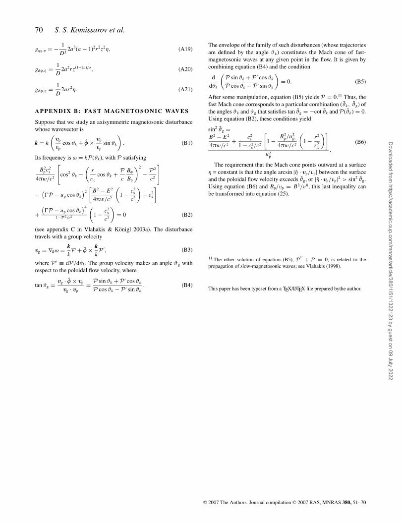
70 S. S. Komissarov et al.
gηη,η = − 1
D32a3(a − 1)2r 2z2η, (A19)
gφφ,ξ = 1
D2a2r z(1+2a)/a, (A20)
gφφ,η = 1
D2ar 2η. (A21)
A P P E N D I X B : FA S T M AG N E TO S O N I C WAV E S
Suppose that we study an axisymmetric magnetosonic disturbancewhose wavevector is
k = k
(vp
vpcos ϑk + φ × vp
vpsin ϑk
). (B1)
Its frequency is ω = kP(ϑk), with P satisfying
B2p c2
s
4πw/c2
[cos2 ϑk −
(r
rlccos ϑk + P
c
Bφ
Bp
)2
− P2
c2
]
− (�P − up cos ϑk
)2[
B2 − E2
4πw/c2
(1 − c2
s
c2
)+ c2
s
]
+(�P − up cos ϑk
)4
1−P2/c2
(1 − c2
s
c2
)= 0 (B2)
(see appendix C in Vlahakis & Konigl 2003a). The disturbancetravels with a group velocity
vg = ∇kω = kkP + φ × k
kP ′, (B3)
where P ′ ≡ dP/dϑk . The group velocity makes an angle ϑg withrespect to the poloidal flow velocity, where
tan ϑg = vg · φ × vp
vg · vp= P sin ϑk + P ′ cos ϑk
P cos ϑk − P ′ sin ϑk. (B4)
The envelope of the family of such disturbances (whose trajectoriesare defined by the angle ϑ k) constitutes the Mach cone of fast-magnetosonic waves at any given point in the flow. It is given bycombining equation (B4) and the condition
d
dϑk
(P sin ϑk + P ′ cos ϑk
P cos ϑk − P ′ sin ϑk
)= 0. (B5)
After some manipulation, equation (B5) yields P = 0.11 Thus, thefast Mach cone corresponds to a particular combination (ϑk, ϑg) ofthe angles ϑ k and ϑg that satisfies tan ϑg = −cot ϑk and P(ϑk) = 0.Using equation (B2), these conditions yield
sin2 ϑg =B2 − E2
4πw/c2+ c2
s
1 − c2s /c2
[1 − B2
p /u2p
4πw/c2
(1 − r 2
r 2lc
)]u2
p
.
(B6)
The requirement that the Mach cone points outward at a surfaceη = constant is that the angle arcsin |η · vp/vp| between the surfaceand the poloidal flow velocity exceeds ϑg, or |η · vp/vp|2 > sin2 ϑg.Using equation (B6) and Bp/vp = B η/vη, this last inequality canbe transformed into equation (25).
11 The other solution of equation (B5), P ′ ′ + P = 0, is related to thepropagation of slow-magnetosonic waves; see Vlahakis (1998).
This paper has been typeset from a TEX/LATEX file prepared bythe author.
C© 2007 The Authors. Journal compilation C© 2007 RAS, MNRAS 380, 51–70
Dow
nloaded from https://academ
ic.oup.com/m
nras/article/380/1/51/1322123 by guest on 09 July 2022
Copyright © 2022 FDOKUMEN