ACCELERATION ALGORITHMS FOR PROCESS ... - ShareOK

ACCELERATION ALGORITHMS FOR

PROCESS DESIGN

SIMULATIONS

by

ANOUSHTAKIN ARMAN ff

Bachelor of Science in

Chemical Engineering

Oklahoma State University

Stillwater, Oklahoma

May, 1985

Submitted to the Faculty of the Graduate College of the

Oklahoma State University in partial fulfillment of

the requirements for the Degree of

MASTER OF SCIENCE December, 1986

ACCELERATION ALGORITHMS FOR

PROCESS DESIGN

SIMULATIONS

Thesis Approved:

Dean of the Graduate C:o ege

1263914

ii

ABSTRACT

Direct Substitution Methods for convergence in simulation

software are often slow and time consuming. Convergence can

be speeded up using an acceleration algorithm. Three accel

eration algorithms were tested on MAXISIM, a chemical pro

cess design simulation package developed at Oklahoma State

University. The algorithms tested were Wegstein's Method,

Dominant Eigenvalue Method (DEM), and the General Dominant

Eigenvalue Method (GDEM). Eight process models were tested

ranging from non-oscillatory to very oscillatory systems

using a variety of combinations of chemical process units at

different conditions.

The best result was found using GDEM, ranging from no

improvement for the very oscillatory systems to over 90 %

reduction in the number of iterations in the case of a non

oscillatory system. An average saving of 45 % in cpu time

can be achieved for a typical process model.

iii

ACKNOWLEDGEMENTS

I wish to express my sincere gratitude to all the people

who helped me in this work at Oklahoma State University. In

particular, I am indebted to my principal adviser, Dr. Ruth

C. Erbar for her guidance, encouragement, and moral support

to continue on the path of education. I am also thankful to

Dr. J. Wagner and Dr. M. Seapan for taking on the task and

the responsibility as my committee members.

The presence and the help of Danny Friedemann and Carlos

Ruiz on computers was especially appreciated. Also my deep

est appreciation goes to the School of Chemical Engineering

at Oklahoma State University for the financial support I

received during the course of this work.

lV

TABLE OF CONTENTS

Chapter Page

I . INTRODUCTION. . . • • . • . . . . . . . . . . . • . . • . . . • . . . . . . . • . . . 1

II. LITERATURE SURVEY:NUMERICAL METHODS............. 5

Direct Substitution..................... 5 Wegstein's Method....................... 6 Dominant Eigenvalue Method.............. 8 General Dominant Eigenvalue Method ...... 11 Newton and. Quasi-Newton's Methods ..•.... 14

II I. DISCUSSION AND RESULTS.......................... 17

IV. SUMMARY, CONCLUSIONS, AND RECOMMENDATIONS .....•. 46

Summary and Conclusions .....••..•....... 46 Recommendations for Further Study ....... 49

L I TE RA TURE C I TED . • . . • . . . • . . . • • . • • . . . . . • . • • . . • . . . . . . . . . • 50

APPEND I XES . . . . . . . . . . . . . • . . • . • . . • . . . . . . . . . • . . • • . • • . . . . . . 52

APPENDIX A - BEHAVIOR OF THE MATRIX NEAR THE SOL UTI ON • ..••.•.•.•....••..••.....•

APPENDIX B - OPTIMIZING THE PERFORMANCE OF THE WEGSTEIN'S METHOD. . ...............

APPENDIX c - OPTIMIZING THE DEM • ••••••••••••••.•

APPENDIX D - FLOWCHART OF THE GDEM ACCELERATION

53

56

60

ALGORITHM. . • • . • . . • . • • • • • • . • . . . • . • . • 6 3

APPENDIX E - COMPOSITION AND THE CONDITIONS OF THE INPUT STREAMS IN THE PROCESS MODELS .........••.......... 65

APPENDIX F - CHARACTERISTICS OF THE DISTILLATION UNIT IN MODEL 7 . . . . . . . . . . . . . . . . . . . . 6 6

APPENDIX G - CHARACTERISTICS OF THE DISTILLATION UNIT IN MODEL 8 (A) ................ 67

v

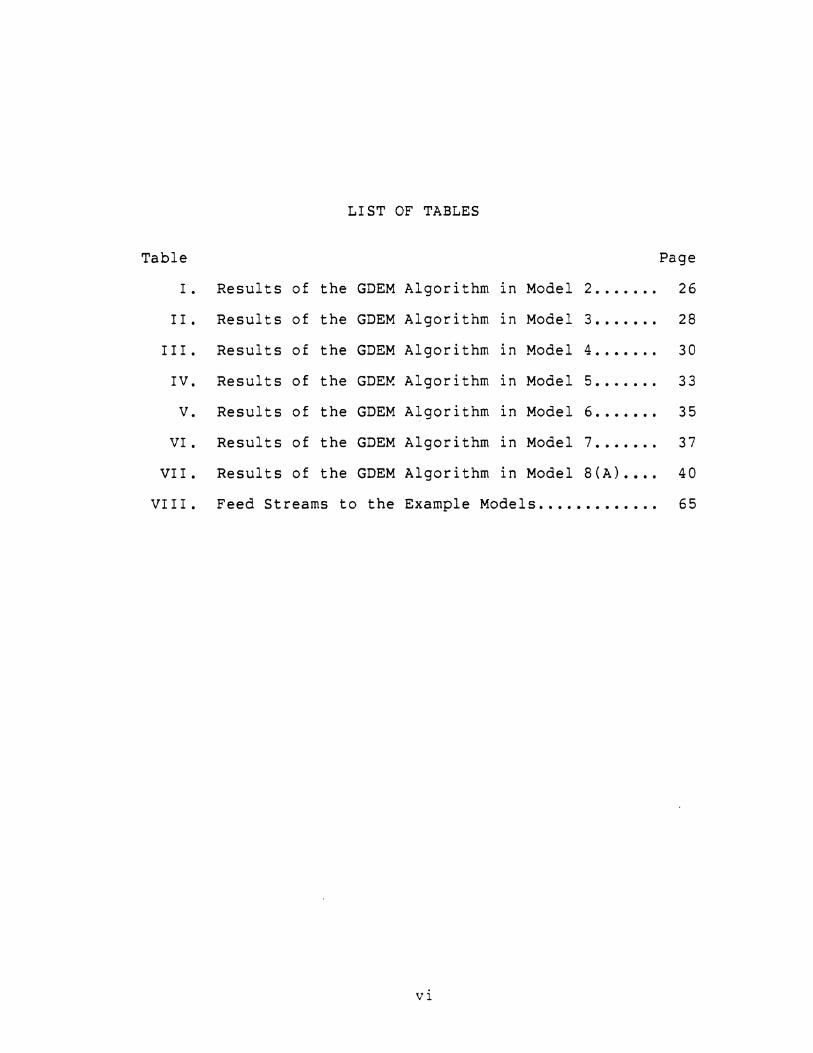
LIST OF TABLES

Table Page

I. Results of the GDEM Algorithm in Model 2 ••••••• 26

II. Results of the GDEM Algorithm in Model 3 ••••••• 28

I I I. Results of the GDEM Algorithm in Model 4 ••••••• 30

IV. Results of the GDE~ Algorithm in Model 5 ••••••• 33

v. Results of the GDEM Algorithm in Model 6 ••••••• 35

VI. Results of the GDEM Algorithm in Model 7 ••••••• 37

VII. Results of the GDEM Algorithm in Model 8 (A) •••• 40

VI I I. Feed Streams to the Example Models ••••••••••••. 65

Vl

LIST OF FIGURES

Figure Page

1. Sequential Modular Architecture................... 2

2. Graphical Illustration of the Wegstein's Method... 7

3. The Pipe Network •••.•.•..••...•••••.•••..•.•.••..• 18

4. Comparison of the Three Methods in the. Pipe Network............................... 21

5. A Typical Chemical Process Model ..••••.••..•••..•. 22

6. Comparison of the Three Methods in Model 2 •..•..•. 23

7. A Heat Exchange Dominated System ..•••...••••.•.... 27

8. A Heat and Mass Dominated System ..•....•.•.•.•..•. 29

9. A Stream Divider Dominated System •......•....•..... 32

10. A Flash Dominated System.......................... 34

11. System Containing a Distillation Column ••.......•. 36

12. System With Four Flash Drums in Series ....•.....•. 38

13. Oscillatory Behavior of Flash Drums in Series •.... 41

14. Distillation Column Replacing Flashes in Series ... 42

15. Stability of Stream# 4 in Model 8 (B) ....•..•.... 43

16. History of the Sum of the Mass of Stream #3 ....... 54

17. Oscillatory History of the Sum of the Mass 0 f s t ream # 4 ... 0 • • • • • • • • • • • • • •••• ., • • • • e • • • • • • • • • • • 55

18. Optimizing q in the Bounded Wegstein •..•...•...... 57

19. The Effect of Temperature on the Convergence of Wegstein....................................... 58

20. Wegstein Applied Every Other Iteration ............ 59

21. Orbach and Crowe's DEM Applied at Different AA ... 61

vii

22. Orbach and Crowe's DEM Applied at Different Damping Factors................................... 62

23. Flowchart for the GDEM Algorithm ..••.••.•..••..... 64

Vlll

LIST OF SYMBOLS

A - Linearized approximation to F

E - Accuracy desired

F(X) - Feed stream

FR - Calculated feed of a broken recycle stream

H - The negative inverse of the Jacobian matrix

I - The identity matrix

PR - Calculated product of a broken recycle stream

T - The transpose matrix

W - Weighting matrix

X - Feed stream to a process unit

e - An arbitrary point near n

n - Number of iterations performed

o - The initial guess

s - The absolute solution ·1'-

v - Number of coefficients to estimate ,f"- j

- Damping factor in DEM

- Eigenvalue of A

- Forward difference operator ,,

_,P-j - jth eigencoefficient of A

- Estimated value

- Temperature, F

- Pressure, psia

- Stream number

ix

CHAPTER I

INTRODUCTION

A steady state process design simulation is a mathemati

cal model representing a process. The independent variables

or the specified conditions are identified and the dependent

variables are calculated.

In a process simulation with no recycle streams the cal

culation is usually straight forward. The calculations on

each process unit are done individually and sequentially and

the process is completed in one iteration (Figure l(A)).

However a process with one or more recycle streams necessi

tates the use of an iterative procedure for convergence.

The convergence criterion is usually a specified tolerance

in the change of properties and/or rates between two sequen

tial iterations on the recycle stream (9). Most process

simulators use the sequential modular architecture to estab

lish a logical method for solving for the unknown variables

in the system.

Sequential modular architecture is a concept where the

recycle streams are conceptually broken and treated as prod

ucts, PR, of the originating unit and feeds, FR, to the des-

tination unit. The calculations are performed sequentially

as if no recycle stream exists. This procedure is repeated

1

IPl l F2

Fl = x1 ;l A 1-j--X2-~1 B r-l--x-3-->~~---J

Fl Xl

FRl (estlmated)

FF Xl ~

(A) Process With no Recycle

1' Pl

AI 1---X2--*~

[F3 • Rl

J,F2 _

B ~-I -X3-~> __ I _c--'J P2 >

(B) Process Containing a Recycle Stream

TPl

A ~---1 -X2=---'~>I

FRl (calculated) t F2 t

B I~--=X3,.----:,.t)~ c I PZ )

(C) Process Containing a Recycle Stream Conceptually Broken into Feeds and Products

Fn - External Feed Streams Pn - External Product Streams Xn - Internal Product/Feed Streams

FRn - Recycle Streams

Figure 1. Sequential Modular Architecture

2

3

until the feed and the product agree within a set tolerance

(Figures l(B and C)).

In many instances the process of convergence to the set

tolerance becomes a very time consuming one involving mil

lions of calculations and thus the incentive to use an

acceleration algorithm to accelerate the convergence or

reduce the number of calculations becomes great. The vari

ables for the acceleration algorithm can be the individual

mass flow rates of the components in any stream in the pro

cess, the temperature, pressure, quality or any other prop

erty of the stream that is changing with every iteration.

These variables almost always have a non-linear dependent

relationship with respect to each other that can be likened

to a set of non-linear dependent equations. An example is

the relationship of the feed stream of the process simula

tion to the product streams.

The relationship between the feed, X, and a product

stream, F(X), can be mathematically represented as

F(X) = X (1-1)

In a steady state process simulation the function, F, is

usually too complex to be expressed mathematically. The

problem is to find Xs such that

F(X) = Xs (1-2)

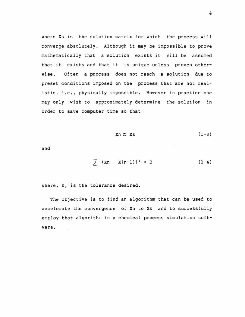
4

where Xs is the solution matrix for which the process will

converge absolutely. Although it may be impossible to prove

mathematically that a solution exists it will be assumed

that it exists and that it is unique unless proven other

wise. Often a process does not reach a solution due to

preset conditions imposed on the process that are not real

istic, i.e., physically impossible. However in practice one

may only wish to approximately determine the solution in

order to save computer time so that

Xn ~ Xs (1-3)

and

~ (Xn- X(n-1)) 2 < E (1-4)

where, E, is the tolerance desired.

The objective is to find an algorithm that can be used to

accelerate the convergence of Xn to Xs and to successfully

employ that algorithm in a chemical process simulation soft-

ware.

CHAPTER II

LITERATURE SURVEY

NUMERICAL METHODS

In recent years there has been a great deal of research

in the area of acceleration algorithms. However, only a few

of these methods will be discussed below. The advantage of

having an automatic means of accelerating the solution in a

computer simulation must be obvious to the reader. A few

specific questions that should be kept in mind when discuss

ing numerical methods are 1) When will the acceleration be

applied ? 2) Is the algorithm stable ? and 3) How much com

puter time can be saved ?

Direct Substitution {D.S.)

In direct substitution the previous value of X is substi

tuted in the function vector

X(n+l) = F(Xn) (2-1)

This method is not really an acceleration algorithm at all

and is often very slow to converge. However, direct substi

tution is very stable especially where oscillatory behavior

exists in the system.

5

6

Weastein's Method

Wegstein's method for multivariable programs is a secant

method approximation first proposed by Aitkin (1) where the

new estimate for Xn is estimated as follows

X(n+l) = Xn- F(Xn)(Xn-X(n-1)) I (F(Xn-F(Xn-1))) (2-2)

Aitkin's method was later modified by Wegstein (14) and

Kliesh (9) until Graves (8) proposed the following equiva

lent expression for X(n+l) where the function, F, has been

linearized (Figure 2).

X(n+l) = (1-g) F(Xn) + g Xn (2-3)

where

g = s I (s-1) (2-4)

and

s = (F(Xn) - FX(n-1)) I (Xn- X(n-1)) (2-5)

The advantage of the Graves expression is that a limit

can be set on the parameter g . Note that if Xn = X(n+l) or

if s = l the calculation of X(n+l) becomes impossible. For

various values of g the characteristics of the Wegstein are

g = 0

g < 0

q > 0

successive substitution

can speed convergence but

also introduces instability

slow, stable convergence.

7

F(X)

Xn-1 Xn Xs +

X

Figure 2. Graphical Illustration of the Wegstein's Method

8

All accelerating algorithms assume a linearity of the

matrix near the solution. Although this may be a good

assumption in most cases there are exceptions to this rule

(APPENDIX A}. Note that Wegstein's method is applied to

every variabie in the matrix separately. Thus , ignoring

the interaction between the variables is the biggest defi

ciency of the method. This characteristic of the method can

lead to an oscillatory behavior that can result in the div

ergance of the solution.

The oscillatory behavior of the Wegstein can be partially

corrected by setting an upper and a lower limit on the value

of q •

q (min.} < q < q (max.}

Called the bounded Wegstein,

introducing a damping factor

behavior of the method and

this method is similar to

to counter the oscillatory

thus assure the convergence.

Another detriment of the method is that there are no spe

cific criteria to help determine when the acceleration

should be used.

next chapter.

These problems will be discussed in the

Dominant Eigenvalue Method (DEM}

If the iteration is approximated by a first order Taylor

9

series expansion of equation 2-1 about an arbitrary point,

Xe, in the neighborhood of Xn the linear matrix becomes

X(n+1) = A Xn + b (2-6)

where

A = ( 6 F I ~ X) @ X = Xe (2-7)

and

b = F(Xe) - A Xe (2-8)

Orbach and Crowe's DEM (11) is a convergence scheme based on

the assumption that the largest eigenvalue in A dominates

the solution. It is necessary at this point to introduce a

few definitions. From equation 2-6 the function F(X) can

be expressed as AXn where the eigenvalues of X are defined

such that they satisfy the equality, AXn = Axn where X is

called the eigenvector, ~ is called the eigenvalue of X,

and all the eigenvalues of X are called the eigenrow of X.

If the eigenvalues, )\ j, of A are labeled in descending

order of the absolute magnitude, the only necessary and suf

ficient condition for convergence would be that

(2-9)

where, A 1, is the dominant eigenvalue (7).

The solution to equation 2-6 is in general

n Xn - Xs = A (Xo - Xs) (2-10)

and 1n particular

m

Xn - Xs = L j=l

10

n

Cj Zj A j (2-11)

where Xo is the initial guess and Xs is X at the solution

if all A j are distinct. Here

and T

Cj = Wj

Xs = (I - A) - 1 b

T (Xo - Xs) I (Wj

(2-12)

z j) (2-13)

and Zj and Wj are the eigenvectors and eigenrows of A j.

In a monotonic convergence near the solution equation

2-11 becomes approximately a geometric progression of the

solution of the form

n

Xn - Xs = C1 Zl A 1 (2-14)

From equation 2-14 it can be shown that n-1

6 Xn :: Xn - X(n-1) = C1 Z1 ( ( A 1) - 1 ) A 1 (2-15)

and that the ratio of the two norms becomes

I A 1 I = II A Xn II I II A X(n-:) II (2-16)

Combining equations 2-14 and 2-15 the apparent solution

becomes

X ( n + 1 ) = X ( n -1 ) + 0{ ( Xn - X ( n -1 ) ) I ( 1 - A 1 ) ( 2 -1 7 )

11

where tX is the damping factor i nt reduced to the equation to

suppress oscillation. Note that if A 1 is close to unity

the correction becomes very large and convergence very slow.

Also if A 1 < 0 the correction falls between Xn and X(n-1).

The only

being -1 A 1

necessary condition in DEM for convergence

< 1 . The stability of the method would then

be directly proportional to the stability of A 1 . Orbach

and Crowe (11) recommended the percentage change of A as a

measure of stability for the algorithm where

6 A = (A n - A (n-1)) 100 I A (n-1) (2-18)

Thus the criteria for acceleration become that I A 11< 1 and

that two successive eigenvalues differ by no less than a

preset value, AA.

General Dominant Eigenvalue Method (GDEM)

Crowe and Nishio (5) proposed a more effective conver

gence promotion also based on the eigenvalues of the solu-

tion matrix. Starting with the basic linear form of equa-

tion 2-6 in terms of the forward differences

Xn = A X(n-1) (2-19)

The characteristic equation of A is

m

IAI-At='l ~j j=O

12

m-j

~ = 0 (2-20)

where m is the dimension of the matrix and/"' j 1s the eigen

coefficient. Also,

j

/j = (-1) l. Ail f.i2 ••• "ij (2-21)

where

1 < j < m

1 < il < i2 < ••• < ij < m

and

~0 = 1

From the Cayley-Hamilton theorem (10), A satisfies equation

2-20 so that m m-j

2 ~ j A A X(n-m) = 0 j=O

Repeated use of equations 2-19 and 2-22 gives

m

~ /j Ax(n-j) = 0

j=O

(2-22)

(2-23)

If the eigenvalues are labeled in ascending order of magni-

tude and if we assume that only v of them were large enough

to dominate the iteration, it then follows that

m

L /j AX(n-j) = 0

j=v+l

(2-24)

13

The iteration is thus confined to a v dimensional sub-

space. An approximation to equations 2-22 and 2-23 gives

where

....

v

~ ~ J A X(i-j) = 0 jf;,O /

i = n , (n+l) , ...

(2-25)

and~ J is an approximation to the real value of ~ j.

Also~ j is estimated by taking the derivative of the square

norm with respect to~ k and setting them equal to zero.

Thus

where

and

v

} ;. . bj k = 0 foo ./ J

k = 1 ,2 , ... ,v

bij = <A X(n-j) , A X(n-k) >

The inner product, < X,Y >, is defined by

T

< X,Y >=X Wy

(2-26)

(2-27)

(2-28)

where W is the weighting matrix, usually the identity ,..

matrix. Xs is the limit to convergence as Xn approaches

infinity.

Thus equation 2-25 becomes

o- Oo ,.. Xs - X(n+l) = "f. A Xi

i=n+l L A X( i-j)

i=n+l .(2-29)

14

Rearranging equation 1-29

v v

{s = Z, / j X ( n + 1- j) I l; j J=O j=O

(2-30)

For V = 1, equation 2-30 reduces to

Xs = Xn + A Xn I ( 1 + /" 1 ) (2-31)

where

bOl I bll (2-32)

A

Orbach and Crowe used A 1 = (bOO I bll)ll 2 from the Cauch-

y-Schwartz inequality , .. ... 1/-1 rl I < (2-33)

for convergence. Thus with GDEM we have avoided the use of

a damping factor and can use the full promotion step of the

accelerator. A similar criterion for acceleration was used ,..

for GDEM as for DEM where, Ll~ is defined

,.. " .... l::t)" = (_/"n -,r(n-1)) 100// (n-1) (2-34)

Newton and Quasi-Newton Methods

The classical approach to solving non-linear simultaneous

equations is the Newton method where the solution of the

equations of the form

F(X) = 0 (2-35)

is

X(n+l) = Xn- Jn-l F(Xn) (2-36)

15

where Ji is the Jacobian matrix of the first partial deriva

tives, ( ~ F(X)/ ~X), evaluated at Xn (4). As was men

tioned earlier the exact value of the Jacobian is almost

never known in a process simulation. Therefore the Jacobian

is usually approximated by the first difference of the

matrix.

Quasi-Newton methods emerge as techniques to evaluate and

update the Jacobian. In the Broyden's Method (2) the Jaco

bian is updated as follows;

H(n+l) = Hn- ((Hn Yn- Qn) Pn I Pn Yn )

where

Hn =- Jn- 1

Pn = Hn Qn

Qn = X(n+l) - Xn

and

Yn = F(X(n+1)) - F(Xn)

(2-37)

(2-38)

(2-39)

(2-40)

(2-41)

Soliman (13) describes variations to equation 41 which

are simpler, more efficient, and require less computer stor

age. These variations of Quasi-Newton methods can be

divided into two categories. One in which the Jacobian is

assumed to be the identity matrix and the other where the

Jacobian is approximated by the first difference of the

matrix. In the first category of the Quasi-Newton methods

the improvement over the eigenvalue methods is not consider-

16

able. In the second category, although there is a consider

able improvement made in convergence, there are however two

disadvantages. 1) m iterations are necessary to determine

the first approximation to the Jacobian. Thus for a fifty

variable matrix fifty iterations will be required before a

next guess could be made. 2 ) Considerable amount of com

puter time and storage will be necessary to store and invert

the Jacobian. For these reasons Quasi-Newton methods will

not be discussed as suitable candidates for the acceleration

algorithm.

CHAPTER III

DISCUSSION AND RESULTS

To give the reader a sense of the relative strength of

the acceleration algorithms a simple nonlinear classical

problem called the Pipe Network was chosen. The algorithms

tested were the Bounded Wegstein, DEM, and GDEM against

Direct Substitution (DS). Process Model 1 or the pipe net-

work consists of 5 horizontal pipes with 5 nodes (Figure 3).

The pressure drop is given by the fanning equation (3)

Pi - Pj = Fm ~ Urn 2 L 12 D (3-1)

where, Fm is a dimensionless moody friction factor, ;0 is

the liquid density, Urn is the mean velocity and L and D are

the length and diameter of the pipe respectively.

flow rate, Q, where

Q = ( 1T D 2 I 4 ) Urn

Equation 3-1 becomes

Pi - Pj = 8 Fm .f Q2 L I TT 2 D5

= c L Q2 I Ds

Given a

(3-2)

(3-3)

(3-4)

where, C is a constant. Note Fm can be assumed constant in

highly turbulent regions (i.e. low C values).

17

MODEL 1

~--------------~~2 _________ 3

4 5

Cl2 = C23 = 3.7326E-4

Cl4 = C45 = C52 = 5.905E-5

Pl = 50 P3 = 0

Initial estimates of pressures are

P2 = 20 , P4 = 40 , PS = 30

Figure 3. Tne Pipe Network

18

19

Let

Cij = C Lij I Dij 5 (3-5)

then

I Pi - Pj I= Cij Qij 2 (3-6)

where Qij is the flow rate between the nodes i and J. Equa

tion 3-6 can be rearranged and since the sum of the flow

rates is zero at any node,

Qij = (Pi- Pj) (1 I (Cij I Pi-Pj )) 1 1 2 = 0 (3-7)

Equation 3-7 can be rearranged to give

Pj = { Aij Pi I 2. Aij (3-8)

where

Aij = (Cij I Pi - Pj ) 1 / 2 (3-9)

The trial and error computation is performed as follows.

An estimate of Aij is made using the previous values of the

pressure at the nodes using equation 3-9. Then a new esti

mate of the pressure can be made by using equation 3-8.

Fi = Pj - A .. o· I l J • l 1 L Ai j (3-10)

where Fi approaches zero as the solution converges. The

error is estimated by the equation;

E = F2 2 + F4 2 + F5 2 (3-11)

20

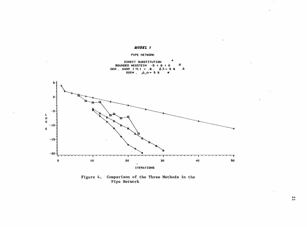
The results of each method is plotted in Figure 4. Weg-

stein's and DEM were optimized for best results (APPENDIX B

and C). The results basically duplicate the findings of

Soliman (13) where GDEM shows the best convergence of the

problem.

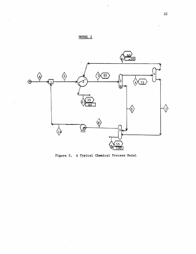
The first step in finding the best acceleration algorithm

is to find a typical chemical process ~odel that can be rep

resentative of the type of models used in chemical engineer

ing. All the che~ical process models were tested using

MAXISIM, a process design simulation package developed at

Oklahoma State University (6). Process Model 2 is such a

model, actually part of a real process system modified for

our purposes (Figure 5). For Wegstein's method Q is damped ,...

between 0 and -5, for DEM. 0(, = 0. 9 and A A = 5%, and for ,..

GDEM A~= 5%. The stream accelerated is # 3 where the

error or the tolerance in the process simulations is defined

as

E = A X I = L (X(i,n)- X(i,n-1)) 2 (3-12)

The results of the model 2 calculations are plotted in Fig-

ure 6. Again GDEM shows the best results. In fact the best

for GDEM were obtained using ...

results AJA = 1%. The percent-

in the eigencoefficient, 1\

is in reality a age change A)" ' measure of how accurate the next estimate will be. For

" example, a large A~ means the acceleration will be

5

0

-5 L 0 G

-to E

-15

-20

0 tO

MODEL t

PIPE NETWORK

DIRECT SUBSTITUTION BOUNDED WEGSTEIN -5 < 0 < 0

+

OEM . DAMP I 0(. I m • 9 A ).. a 5 :110

GDEM . 4/-'-• 5 :110 *

20 30

ITERATIONS

J]

A

Figure 4. Comparison of the Three Methods in the Pipe Network

T --.----~r--.--,--y--r-.~

40 50

N ,_.

22

MODEL 2

Figure 5. A Typical Chemical Process Model

L 0 G

E

JIODEL 2

STREAM f 3

DIRECT SUBSTITUTION + BOUNDED WEGSTEIN -5 < 0 < 0 -It

OEM • DAMP C C( I • • 9 • tl A • 5 X 0 GDEM • Jj ~ • 5 X 6

2 "1 0.0

~ -2.5

-5.0

-7.5i ~ 1 u a I o u a I u u 1 a u u a u u u a u 1 u 1 a a a a u ; ; 1 u ; ; u a u u s u I ; a u a ; o 0 u 1 I

0 5 10 15 20 25

ITERATIONS

Figure 6. Comparison of the Three Methods in Hodel 2

N w

24

attempted before the eigenvalue has stabilized. Conse-

quently the estimate will be less accurate as opposed to

' that from a smaller ~-~ which means the acceleration will be

delayed several iterations but the estimate will be more

accurate. This is a question of trade off which will be

discussed later in more detail.

In Chapter I some of the individual variables mentioned

which could be used 1n an acceleration algorithm were the

individual mass flow rates, the system temperature, pres-

sure, quality, enthalpy, and entropy , etc •. Gibbs theorem

(12) states that all the properties of a system are com

pletely determined given the composition and two independent

variables in the system. The simulation package, MAXISIM

has a built in flash operation that can determine the sys

tem's condition completely given the composition, tempera-

ture, and pressure. Since all process unit operations on

MAXISIM are performed isobarically (i.e. at constant pres

sure) this leaves only one independent variable that could

be used in the acceleration algorithm. Therefore, the log-

ical choice for the individual variables in the acceleration

algorithm were the individual flow rates and the stream

temperature. Note that to have increased the variables in

the acceleration by another independent variable would have

over defined the system causing thermodynamic inconsisten-

cies.

The logical steps of how a typical acceleration algorithm

like GDEM would interact with the main simulation software

25

1s shown in the form of a flowchart in APPENDIX D. The com-

position and the conditions of the feed streams to the chem

ical simulations are listed in APPENDIX E.

At this point several questions needed to be answered.

1) How to choose the stream to be accelerated ? 2} Is there ,..

an optimum value for AJA? , and 3} How GDEM would perform

against a more oscillatory system ?

Table I shows the results of Model 2 computations. The

best result was a convergence in 11 iterations " with A)'"=

1%. Almost a 50% reduction in number of iterations and 45 %

reduction in computer time over direct substitution. Six

more models each with some specific characteristics were

chosen to further test GDEM •

Model 3 is basically a heat exchanger dominated system

where only heat is transfered to the feed stream (Figure 7).

Although Model 3 shows no oscillation, very little mass is

recycled to the heat exchanger reducing the effect of the

acceleration resulting in only a 15% reduction in number of

iterations (Table II}.

Model 4 is a combination of heat and mass transfer domi-

nated system where only one stream is recycled through the

heat exchanger and another recycled through a flash opera-

tion (Figure 8). This model shows a surprising degree of

oscillation such that acceleration could not be attempted

resulting in no improvement over D.S. (Table III).

26

TABLE I

RESULTS OF THE GDEM ALGORITHM IN MODEL 2

A.

STREAM ! A p- (!) ITERATIONS

2 5 13

2 1 11

3 5 12

3 1 11

4 5 13

6 5 21

7 5 14

10 5 13

10 1 11

Tolerance = lE-4

Direct Substitution = 21 Iterations

Method = GDEM

27

Figure 7. A Heat Exchange Dominated System

STREAM !

2

8

TABLE II


5

5

Tolerance = 1E-5


Method = GDEM

28

ITERATIONS

11

11

29

MODEL 4

Figure 8. A Heat and Mass Dominated System

STREAM .!

2

4

6

10

.TABLE III


5

5

5

5

Tolerance = 1E-5


Method = GDEM

30

ITERATIONS

14

14

14

14

31

Model 5 is a stream divider dominated system with only

one recycle stream through a flash operation (Figure 9). A

stream divider is the simplest form of an unit operation

where all the characteristics of the stream remain intact

while the mass flow rate is divided. In Model 5, the stream

has been divided into a 10% to 90% ratio in mass flow rate.

The non-oscillatory behavior of this model lends itself very

nicely to acceleration algorithms. The results of Model 5

calculations are tabulated in Table IV with almost a 90%

reduction in the number of iterations compared to direct

substitution.

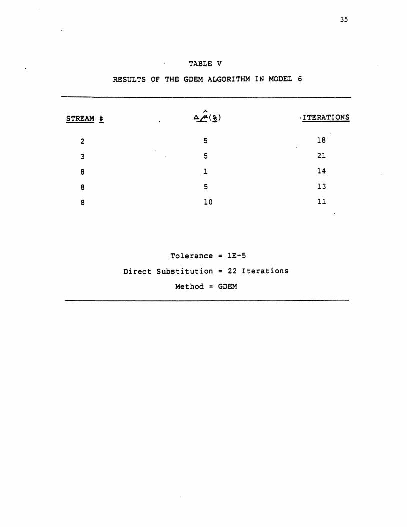
Model 6 is a purely flash dominated system with only one

recycle stream (Figure 10). Also a very typical chemical

process model, the 'best results for Model 6 were obtained A

accelerating the recycle stream and A~= 10% with a conver-

gence in 11 iterations with a 50% saving in the number of

iterations (Table V).

Model 7 introduces a distillation column connected to

three flashes with one recycle stream (Figure 11). This

model like Model 4 showed a surprising degree of oscillation

which translates into zero improvement in convergence over

D.S. (Table VI). Note that Process Model 7 is not a realis-

tic representation of a process system and is introduced

here purely for academic reasons to test GDEM against oscil-

latory systems.

Model B(A) is a more complicated system with 6 recycle

32

MODEL 5

Figure 9. A Stream Divider Dominated System

STREAM !

3

3

6

6

TABLE IV


5

1

5

1

Tolerance = lE-5


Method = GDEM

33

ITERATIONS

10

10

12

12

34

MODEL 6

Figure 10. A Flash Dominated System

35

TABLE V


II>

STREAM ! A_e(!) ·ITERATIONS

2 5 18

3 5 21

8 1 14

8 5 13

8 10 11

Tolerance = 1E-5


Method = GDEM

36

MODEL 7

Figure 11. System Containing a Distillation Column

*APPENDIX F

STREAl~ !

10 10

TABLE VI


Tolerance = lE-5 Direct Substitution = 15 Iterations

Method = GDEM

37

ITERATIONS

15 15

38

MODEL 8(A)

Figure 12. System With Four Flash Drums in Series

39

strea~s (Figure 12). This model would normally be used in

the latter stages of a typical design process. A closer look

at Model 8(A) will reveal that units 5, 7, 8, and 9 are con-

nected in series simulating a distillation column where the

heat source for the reboiler duty is supplied by feed stream

#2 at heat exchanger unit 2. It was not very surprising to

find that this model also was very oscillatory because of

the high degree of complexity of the model (Table VII).

Figure 13 shows the oscillatory behavior of stream #4 in

Model 8(A).

The assumption of linearity near the solution is an impor-

tant condition for acceleration algorithms. In the case of

Model 8(A) this condition was not met therefore it is no ~

surprise that the % change in eigencoefficient, ~~ , was

very unstable which means that no acceleration could have

been attempted.

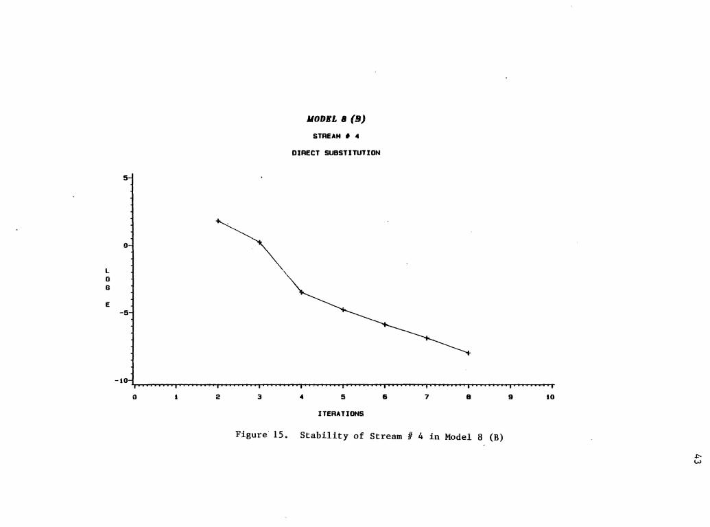
Flash units 5, 7, 8, and 9 can be replaced with a distil

lation column of equal characteristics (i.e. the same sepa-

ration of the light and heavy key components) and heat

exchanger unit 2 can be replaced with a heater/cooler unit

removing heat of equal duty as the reboiler in the distilla-

tion column. Thus Model 8(B) is created from Model 8(A)

where the distillation column has replaced the flash opera-

tions 5, 7, 8, and 9 (Figure 14). With D.S. Model 8(B) con

verges in only 8 iterations as opposed to 33 for Model B(A).

The quick convergence of the system renders the acceleration

algorithm useless (Figure 15). However, note that the

40

TABLE VII

RESULTS OF THE GDEM ALGORITHM IN MODEL 8(A)

STREAM!

10

16

1

1

Tolerance = lE-4


Method = GDEM

ITERATIONS

33

33

2.5

0.0

-2.5 L 0 G

J/ODBL B (A)

STREAM f -4

DIRECT SUBSTITUTION

• ~ool \ v \ -7.5

-SO.Oi V I I I I I I I • • I 1 • 1 1 • • • • 1 1 1 ; a o a 8 1 11 1 1 1 ; ; e ; a 1 ; a ; 1 ; ; e ; e 6 1 1 1 I ; 1 1 1 ; 1 1 1 1 I

0 5 so 15 20 25 30

ITERATIONS

Figure 13. Oscillatory Behavior of Flash Drums in Series

..... ....

42

MODEL 8(B)

~--T"'------1* 5

Figure 14. Distillation Column Replacing Flashes in Series

*APPENDIX G

** -112.43 KBTU/Hr

l 0 G

E

JIODEL B (B)

STREAM f 4

DIRECT SUBSTITUTION

5

0

\

-5

-101 ~~~O~OTO~i~O~O~O~iTO,j~O~i~OTO~O~rT,j~O~O~O~OTO~O~O~O~OTjTO~O~O~i~OTO~O~O~OrTjTO~O~O~OrTOTO~O~O~O~jTOTO~O~O~i~OTO~O~O~jrTOTO~O~O~OTOTOTO~O~jrrCTITS~i~OrTITiTI~S~jrr>TOTO~O~O~ITOTO~O~jrrOTITO~O~I~OTOTITO~j

0 1 2 3 ... 5 6 7 8 9 10

ITERATIONS

Figure 15. Stability of Stream II 4 in Model 8 (B)

~ w

44

information about the reboiler duty and the column charac

teristics about Model 8(B) were known only after Model 8(A)

had converged to a solution. although Model 8(A) and S(B)

have similar separation characteristics, Model 8(B) shows

much less oscillation because the flash operations imbeded

in the distillation column converge iteratively before the

next operation can be performed. Secondly heater/coolers

have a fixed heat load unlike heat exchangers that can have

variable heat loads that change with changing flow rates.

It was found from the example process models that there

are no clear cut criteria to determine the best stream for

acceleration.

worked best.

In most cases the outermost recycle stream

One exception to this rule was found in pro-

cess model 5 where a branched stream had a slight advantage

over the recycle stream. Note that the roles could easily

have been reversed in favor of the recycle stream if some of

the preset conditions in the system were changed. Also in

" most cases a value of A,P- = 1 % seemed to work best although

again an exception was found in process model ,..

6 where Af =

10 % gave the best results.

The reduction in cpu time (computer time) is not always

proportional to the reduction in the number of iterations.

As the system approaches convergence the cpu time for each

iteration usually decreases. Therefore, the actual saving

in computer time will always be a little less than the pro-

portional reduction in the number of iterations. For exam-

ple, as was said earlier in Model 2 for a 50 % reduction in

45

the number of iterations, the actual reduction in cpu time

was only 45 %. However, the reduction in iterations should

serve as a good indicator for the actual saving in cpu time.

It should also be said that including the temperature as an

independent variable in the acceleration does not constitute

a significant saving in the number of iterations. However,

it should not slow convergence either because in all the

systems studied the stream temperature has converged rapidly

and did not dominate the ~alculations of the eigenvalue.

Note that if for some reason the temperature in an hypothet

ical process did not stabilize quickly in a stream with a

small flow rate (ie. 10 total moles/hr) the shear size of

the temperature (ie. 200 deg.F) could actually dominate the

eigenvalue and maybe even slow convergence.

CHAPTER IV

SUMMARY, CONCLUSIONS, AND RECOMMENDATIONS

Summary and Conclusions

In a mixture of chemical compounds the interaction

between the different components is very complex and nonli

near. Wegstein's method becomes ineffective as a tool for

acceleration because each individual component is treated

independently of others. Furthermore, there are no logical

criteria for when the acceleration should be applied. It

has been shown that much better results can be obtained if

the stream to be accelerated is treated as a matrix rather

than a series of unknown equations. DEM and GDEM are meth

ods of acceleration based on the eigenvalue of this matrix.

The improvement over Wegstein is two fold. 1) The interac

tion among the components is considered. 2) The criterion

for acceleration is based solely on the stability of the

eigenvalue.

The best results were for GDEM ranging from zero improve

ment for a very oscillatory system to over 90 % reduction in

the number of iterations in the case of an non-oscillatory

system. Model 2 which represented a typical chemical pro

cess had a reduction of almost 50 % in the number of itera

tions.

46

47

To understand why there is such a large difference in

improvement from one system to another, it must be first

understood what makes one system more oscillatory than

another. Of course if the system were understood completely

there would be no need for an acceleration algorithm. How-

ever, there are several guidelines that can help in under-

standing this oscillatory behavior. For example, oscilla-

tion usually increases with increasing number of recycle

streams in the system and/or if the system contains complex

operations like distillation towers as opposed to simple

operations like stream dividers. Other guidelines are more

subtle, like how the unit operations are arranged and the

system preset conditions.

Automation in the acceleration program can be achieved if

a suitable stream can be chosen for acceleration with an

"' appropriate value for ~~ . The distinction between the

advantages in acceleration of one stream over another is

usually based on a prior knowledge or experience with pro-

cess systems. Without such prior knowledge the outermost

recycle stream can be chosen as a suitable candidate for

"" acceleration. It was also found that a value of 1 % for Af

worked best for most systems. "" Higher values for /Jf' can be

chosen only at the risk of oscillating the system at each

acceleration.

In conclusion the best results were based on the GDEM

using a recycle stream for acceleration with an acceleration ,..

criterion of f1i = 1 %achieving a reduction of 50 % in the

48

number of iterations which approximately corresponds to a 45

% reduction in cpu time. Therefore, we highly recommend the

use of the GDEM algorithm to significantly reduce the com

puter usage and cost. We also found GDEM to be highly suit

able and effective as an acceleration algorithm for process

design simulations. It's use is also not confined to the

convergence of process systems but can also be used anywhere

a convergence parameter is needed to be determined itera

tively requiring ten or more iterations, a common character

istics for many chemical equilibria calculations.

49

Recommendations for Further Study

1. Quasi-Newton Methods can be as an alternative to the

GDEM if methods for updating the Jacobian, starting with the

identity matrix can be improved. Soliman (13) recommends

that the convergence can be improved if Pn = -F(Xn) and

Ho =I.

2. Convergence may be improved if instead of starting the

Jacobian as Ho = ~ F(Xn) I~ (Xn) or Ho =I, a partially

determined Ho is used based on a certain criterion. This

criterion might be the highest mass percent of the compo

nents in the stream or the components in the mid-range

between the lightest and the heaviest components.

LITERATURE CITED

1. Aitken, A.C., "On Bernouli's Numerical Solution of Algebraic Equations," Proc. Royal Soc. Edinburgh, 46, 289-305 (1925).

2. Broyden, C.J., "A Class of Methods for Solving Nonlinear Simultaneous Equations," Math. Comp., 19, 577-593 (1965).

3. Carnahan, B., Luther, H.A., and Wilkes, J.O., Numerical Methods," John Wiley, 5, (1969) •.

"Applied 310-320

4. Conte, S.D., and Boor, C.D., "Elementary Numerical Analysis: An Algorithmic Approach," MacGraw Hill Book Company, 79, 223-226 (1980).

5. Crowe, C.M., and Nishio, M., "Convergence promotion in the Simulation of Chemical Processes - the General Dominant Eigenvalue Method," AICHE J., 21, 528-533 (1975).

6. Erbar, J.H., Revised by Erbar, R.C., "MAXISIM,'' SCI 2701 Fox Ledge Lane, RR5, Stillwater, OK. 74074, Tel. (405) 377-4279 (1984).

7. Faddeeva, V.N., "Computational Methods of Linear Algebra," Dover Publications, Inc., New York, 60-62 (1959).

8. Graves, T.R., "An Evaluation of Convergence Acceleration Methods for Chemical Process Recycle Calculations," Ph.D. Thesis, Oklahoma State University, Stillwater (1972).

9. Kliesch, H.C., "An Analysis of Steady State Process Simulations : Formulation and Convergence," Ph.D. Thesis, Tulane University, New Orleans, La. (1967).

10. Noble, B., "Applied Linear Algebra," Prentice- Hall, Englewood Cliffs, N.J., 372-374 (1969).

11. Orbach, 0., and Crowe, C.M., "Convergence Promotion in the Simulation of Chemical Processes With Recycle - the Dominant Eigenvalue Method," Can. J. Chern. Eng., 49, 509-513 (1971).

50

51

12. Smith, J.M., and Van Ness, H.C., "Introduction to Chemical Engineering Thermodynamics," Third Edition, MacGraw- Hill Book Company, 39-40 (1975).

13. Soliman, M.A., "Quasi-Newton Methods for Convergence Acceleration of Cyclic Systems," Can. J. Chern. Eng., 57, 643-647 (1979).

14. Wegstein, J.H., "Accelerating Convergence of Iterative Processes," Comm. Assoc. Comput. Mach., 1 (6), 9-13 (1958).

APPENDIXES

52

APPENDIX A

BEHAVIOR OF THE MATRIX

NEAR THE SOLUTION

The assumption of linearity near the solution is a criti

cal assumption for convergence of a system. As an example,

Figure 16 shows the total mass of stream # 3 in model 2

( See.model 2 discussion on page 17 ). The total mass at a

given iteration is divided by the final mass for easy com

parison.

As can be seen the total mass follows a predictable curve

and is non-oscillatory while approaching linearity near the

solution.

cillatory.

However, not all process simulations are non-os

This is specially true in a series of flashes

with connecting recycle streams simulating a distillation

tower. Figure 17 showes such an oscillatory behavior in

stream # 4, model 8. Note that although it may appear that

the stream is approaching linearity near the solution ,in

actuality the oscillation still exists in a smaller scale

until the whole system converges at iteration # 30.

53

X N

I X s

MODEL 1

STREAM II 3

DIRECT SUBSTITUTION

t .0

O.B

0.7 ~~,-~----~~~~-r-T~--~~~~~~r-r-T-T-~~~~~~~-r-T~~-,~~~~~r-T

0 5 tO 15 20

ITERATIONS

Figure 16. History of the Sum of the Hass of Stream II 3

VI +:--

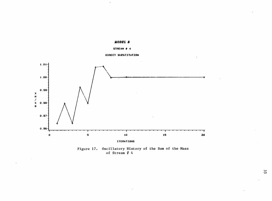
X N I X s

JIODBL B

STREAM • 4

DIRECT SUeSTITUTION

1.01

1.00 ~

0.99

0.98

0.97

0.96~~~~~~---r~-?-.~-,~~~~r-----T-~~,-~~~-r-r-r-r-,~-,~~~~r-r-~T-T

0 5 10 15

ITERATIONS

Figure 17. Oscillatory History of the Sum of the Mass of Stream II 4

20

lJl lJl

APPENDIX B

OPTIMIZING THE PERFORMANCE

OF THE WEGSTEIN'S METHOD

In the optimization of the Wegstein's method model 2 was

used throughout the test. The optimization of the bounded

Wegstein was made by trying to answer the following three

questions. l)What is the best range for q ? 2)How does

including the temperature of the stream affect the conver

gence of the matrix ? And finally 3)Will applying the Weg

stein at every iteration help improve convergence ?

Figures 18, 19, and 20 show that for model 2 the best

range for q is between -5 and 0 • They also show that

including the temperature as a variable in the matrix and

applying Wegstein every other iteration will help improve

the convergence of the method.

56

JIODEL 2

STREAM f 6

DIRECT SUBSTITUTION +

-5 < Q < 0 ~ -5 < Q < 5 0 -10 < Q < 0 ~

5.0

2.5

0.0 L 0 G

-2.5 E

-5.0

-7.5 ljiiliiiUiijilliii iiijiiiiiiillilliiiliililiiliil6 Djiiiiliilljiibiliilli81iliililjiliii iilljfiiiiiiiij

0 2 3 4 5 6 7 B 9 10

ITERATIONS

Figure 18. Optimizing q in the Bounded Wegstein

V1 '-1

L 0 G

E

JIODEL 2

STREAM f 3

DIRECT SUBSTITUTION +

-5 < 0 < 0 (TEMPERATURE INCLUDED) * -5 < 0 < 0 (TEMPERATURE NOT INCLUDEDI D

5.0

2.5

0.0

-2.5

-5.0

-7.5~~,-~~~~-r-r-r~-T-T~~~~~~r-r-r-~T-~,-~~~-r-r-r~~~~-,~~r-r-r-~~

0 5 10 15

ITERATIONS

Figure 19. The Effect of Temperature on the Convergence of Wegstein

20

Vl w

. ·~ 2.5

~ _o.o

L 0 -2.5 G

E -5.0

-7.5

-10.0 T

0

JIODEL 2

STREAM I 6

DIRECT SUBSTITUTION ~

-5 <a< 0 ITEHP.INCLUDED) APPLIED EVERY ITERATION ~ -5 <a < 0 (TEHP.INCLUDED) APPLIED EVERY OTHER ITERATION 0

5 10 15

ITERATIONS

Figure 20. Wegstein Applied Every Other Iteration

20

VI '-0

APPENDIX C

OPTIMIZING THE DEM

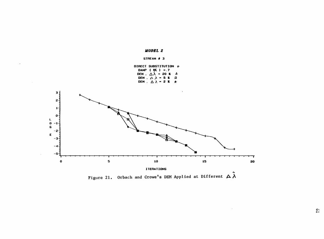
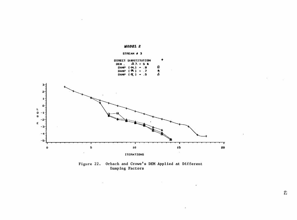
The Orbach and Crowe's DEM ·was optimized based on st-ream

# 3 in model 2. Figure 21 showes no significant difference I florA~ in the range of 2 to 20 %. In Figure 22 a damping

factor of 0.9 shows a slight improvement in convergence.

These findings are in agreement with-the findings of Orbach

and Crowe ( 11) •

60

3-

2

0 l 0 -t G

-2 E

-3

-4

-5 ..,.. 0 5

JIODEL 2

STREAM I 3

DIRECT SUBSTITUTION ~

DAMP I tit I • . 7 OEM . b.A • 20 I A OEM t). )I a 5 I ll OEM, A).,- 2 I fro

so

ITERATIONS

15

~

Figure 21. Orbach and Crowe's DEM Applied at Different ~A

20

0\ .......

3

2

0 L 0 -1 G

-2 E

-3 l -l -5

0

JIODBL 2

STREAM f 3

DIRECT SUBSTITUTION ~ OEM, ,A.). .. 5.

DAMP 1~1 • .9 0 DAMP (Gr.) • .7 !\-DAMP IG(. I • .5 .::\

5 10 15

ITERATIONS

Figure 22. Orbach and Crowe's DEM Applied at Different Damping 'Factors

20

a• N

APPENDIX D

FLOWCHART OF THE GDEM

ACCELERATION ALGORITHM

The following flowchart shows how the series of logical

steps are taken that determines if, how, and when the GDEM

acceleration should be applied (Figure 23) • The first step

is the execution of all unit operations in series. Next if

a recycle stream exists then an iterative procedure would be

followed, otherwise the results are printed and the program

stops. If the pressure is zero very likely the stream is

empty and a warning statement is printed. The contents of

the stream to be accelerated are stored in an array. Three

sets of arraies will be required to store the pressure,

temperature, and the stream composition. In the third iter-

" ation the criteria for the acceleration is checked. If A_lt A

< 1 % and 0 < ~ 2 < 1 are true then the acceleration is

attempted. Stepping back the array is needed to discard the

old stream and enter the new stream values. The flash oper-

ation is necessary after each acceleration to correct the

quality and other thermodynamic properties of the stream.

The simulation is again checked for convergence. If it has

not converged the cycle is repeated until convergence is

achieved.

63

64

Acceleration Flowchart

Iteration • 0

Yes Warning /

I

Yes

No

. xs • Xn +Axn I l •J-'2

No

Figure 23. Flowchart for the GDEM Algorithm

APPENDIX E

COMPOSITION AND CONDITIONS OF THE INPUT

STREAMS IN THE PROCESS MODELS

TABLE VIII

FEED STREAMS TO THE EXAMPLE MODELS

~ ~ (1bmo1e/hr)

C2H6 = 100

N-C4H10 = 80

N-C5H12 = 60

N-C6Hl4 = 40

temperature = 100 (F)

pressure = 100 (psia)

65

FEED B (1bmo1e/hr) ---N2 = 3.47

CH4 = 204.75

C02 = .554

C2H6 = 24.59

C3H8 = 17.47

IC4H10 = 3.457

NC4H10 = 5.224

IC5H12 = 1.689

NC5H12 = 1. 214

NC8H18 = 1.4776

temperature = 100 (F)

pressure = 485 (psia)

APPENDIX F

CHARACTERISTICS OF THE DISTILLATION

!:TXT # : COUNT ?~TES Fn~M BOTTOM UP !IJUMBER OF PLATES IN COLUMN NUMBER OF FEED PI..ATES ~ruMBER OF PRODUCTS

" ... 2

NUMBER OF SIDE CCOLE.!;:S/HEATERS t)

FEED STREAM FEED NO NO PlriTE 1 7

' , 10 8 .;.

PRODUCT STREAM DRAW NO ~0 PLATE

2 14 3

CONDENSER rtPE-TOTL qEBQILER TYPE -PART

DRAW RATE

!),.~41)00

HH+*

cmm8JSER/DISTILLATE SPECiF:CATIONSD:ST!L!..ATE RATE0.64000 iD/Fl

REBOILER:BOTTOMS SPES!FICATIONS-REBOILER DUTY 6. 00 f~:BTULB

UNIT IN MODEL 7

CONVERGENCE PARAI1EiERS NO OF ALLOt~ABLE CONSTANT MOLAL OIJEli:FLQW !TEPf~TIGlS (' t'IAX ALLOWABLE ITERATIONS 2C= MAX DaTA T PER PLATE :o.:;c);j MAX FRACTIONAL LIQ CHANGE PER F-LATE (1, 400

PLATE SPACING TOP SECTION BOT SECTION

24.00 IN 24.;)0 IN

ESTIMATED LIQ RATE LEAVING TOP PL::TE!CCNDENSE~ r:~.:::o = ESTIMATED BOTTOMS RATE 0.:?60 (81Fl

CCLt;MN PRESSURES ;~ ESiiMATED TEMPSATURES P~PSlAl T(DEG Fi

COND8JSER 100. CrO -! 1. :JO TOP p1_~TE ! ':•:. ·)0 FEBO!:..~~· :;:(. ·:·r:· 23.~ •. ~·~)

66

APPENDIX G

CHARACTERISTICS OF THE DISTILLATION

UNIT MODEL S(B)

UNIT OPERATION NO 1 IS A DIST UNITf9*

STREAM FLOW RAiES ARE LB-MOLS STREAM NO 6 7 8

NAME COMPO~JENT

CH4 10.0867 8.4816 1.6051 C2H6. 6.8303 1.4787 5.3516 C3H8 10.6636 0.3238 10.3398 IC4H10 2.7996 0.0183 2.7813 NC4H10 4.5195 0.0161 4.5034 !CSH12 1. o001 :).1)1)12 1.S989 ·~tSH12 1.1680 r), 0005 1.1675 ':C8H18 1.4766 0.1)01)0 1.4766 .. ,., ,.4 .. 1).0466 1).04~4 1),001: .~,,

l..w• (l,Ooo4 f), (•384 0.0280

TOTAL 39.:~:'4 !0.+039 :a.a:3:

T,DEG F -2i),l)f) .. _ ....

- :.•; 1 .jl) 86.5-1-:- per• I II I ...t.N 4:'5,1)0 ~15.00 3!5.t)(\ H,f .. BTU -87.77 32.1)6 -5.~0

S.Y..BT!J/R 1. 7234 0.4061 1.5564 110L ~~EIGHT ·H.6576 19.21:0 49. 75t::: D,LB/FT3 33.7287 1.5420 32.2753 L/F 1MOLARl ! . ·:·i)f)00 1),(\t)l)f)f) l. 0f)c)QI)

MINIMUM ~lUMBER OF STAGES = MINIMUM REFLUX RATE =

NO STAGES REFLUX CONCENSER IN COLUMN RATE DUTY (INC REBl LB-MOLS 10E3KBTU

8.04 1.02 c. (11b 5.36 1.27 r), 019 4.02 I "TQ

A, Ill l I '\ ')24 3.2: 2.74 i:\. (t::3 2.68 -+.-+: '). :•49

67

i. ~1 0.92 ~B-MO:...S

REBOI LEP FEED TRA 'r :JIJTY F'EBO!LER

10E3KBTU =7FA'1 !

o. r:o ~ C• .lo

0.1.::: . ., . ~~'='

i}, !38 • ... .. ( 1,147 • r:

1 ·~ 1;, 1-~: -. -

~ VITA

ANOUSHTAKIN ARMAN

Candidate for the Degree of

Master of Science

Thesis: ACCELERATION ALGORITHMS SIMULATIONS

Major Field: Chemical Engineering

Biographical:

FOR PROCESS DESIGN

Personal Data: Born in Shiraz, Iran, February 20, 1960, The son of Badry Wilfong and Jalil Arman.

Education: Graduated from Cairo American College, Cairo Egypt, in May, 1977; received Bachelor of Science degree in Chemical Engineering from Oklahoma State University in May, 1985 and completed requirements for the Master of Science degree at Oklahoma State University in December, 1986.

Professional Experience: Lab assistant in the chemical and the metallurgical lab, Quality Control Department, Mercury Marine, Stillwater, Oklahoma, May, 1980 to June, 1982.

ACCELERATION ALGORITHMS FOR PROCESS ... - ShareOK

Documents

Transcript of ACCELERATION ALGORITHMS FOR PROCESS ... - ShareOK