arX

iv:0

706.

0897

v1 [

hep-

ph]

6 J

un 2

007

IFIC/07-28

SU 4252-831

Exact relativistic beta decay endpoint spectrum

S. S. Masood,1, ∗ S. Nasri,2, † J. Schechter,3, ‡

M. A. Tortola,4, § J. W. F. Valle,5, ¶ and C. Weinheimer6, ∗∗

1Department of Physics, 2700 Bay Area Blvd.,

University of Houston Clear Lake, Houston, TX 77058, USA

2Institute for Fundamental Theory, University of Florida, Gainesville, FL, USA

3Department of Physics, Syracuse University, Syracuse, NY 13244-1130, USA

4Departamento de Fısica and CFTP, Instituto Superior Tecnico

Avenida Rovisco Pais 1, 1049-001 Lisboa, Portugal

5AHEP Group, Institut de Fısica Corpuscular – C.S.I.C./Universitat de Valencia

Edificio Institutos de Paterna, Apartado: 22085, E–46071 Valencia, Spain

6Institut fur Kernphysik, Westfalische Wilhelms-Universitat Munster

Wilhelm-Klemm-Str. 9; D-48149 Munster, Germany

(Dated: February 13, 2013)

Abstract

The exact relativistic form for the beta decay endpoint spectrum is derived and presented in

a simple factorized form. We show that our exact formula can be well approximated to yield

the endpoint form used in the fit method of the KATRIN collaboration. We also discuss the

three neutrino case and how information from neutrino oscillation experiments may be useful in

analyzing future beta decay endpoint experiments.

PACS numbers: 14.60 Pq, 13.30 -a, 23.40 -s, 23.40 Bw

Keywords:

∗Electronic address: masood@uhcl.edu†Electronic address: snasri@ufl.edu‡Electronic address: schechte@phy.syr.edu§Electronic address: mariam@cftp.ist.utl.pt¶Electronic address: valle@ific.uv.es∗∗Electronic address: weinheimer@uni-muenster.de

1

I. INTRODUCTION

The discovery of neutrino oscillations [1, 2, 3, 4, 5] probes the neutrino squared mass

differences and mixing angles [6], but leaves open the issue of what is the absolute scale of

neutrino mass. The latter has important cosmological implications in the cosmic microwave

background and large scale structure in the Universe, as already indicated by the sensitivities

reached, for example, by the recent WMAP-3 [7], the 2dF Galaxy Redshift Survey [8] and

Sloan Digital Sky Survey results [9]. One expects even better sensitivities in the next

generation of cosmological observations [10, 11]. Interesting as these may be, there are

essentially only two ways to get insight into the absolute scale of neutrino mass in the

laboratory: searches for neutrinoless double beta decay [12] and investigations of the beta

spectra near their endpoints [13, 14, 15, 16, 17, 18]. For the latter direct search for the

neutrino mass a very low beta endpoint is crucial: tritium was used in the most sensitive

spectrometer experiments [14, 15] and rhenium in the up-coming cryobolometer experiments

[19].

Currently a next generation tritium beta-decay experiment is being prepared, scaling up

the size and precision of previous experiments by an order of magnitude, and increasing

the intensity of the tritium beta source: the KArlruhe TRItium Neutrino experiment KA-

TRIN [13, 16, 17, 18]. Such an improved sensitivity experiment will probe neutrino masses

ten times smaller than the current limits and therefore play a crucial role in probing for

direct effects of neutrino masses.

Prompted by the prospects that high sensitivities can be achieved in the next generation

of high precision neutrino mass searches from tritium beta decay experiments [16, 17] we

reexamine the accuracy of the kinematical formulae used in the determination of neutrino

masses from the shape of the endpoint spectrum. We also discuss the interplay of neutrino

oscillation data and the expectations for the beta decay endpoint counting rates for the

different types of neutrino mass spectra.

II. RELATIVISTIC BETA DECAY KINEMATICS

In what follows we label the relativistic momenta and energies involved in tritium beta

decay according to

3H(0, M) →3 He+(p′, E ′) + e−(pe, Ee) + νe(pν, Eν). (1)

2

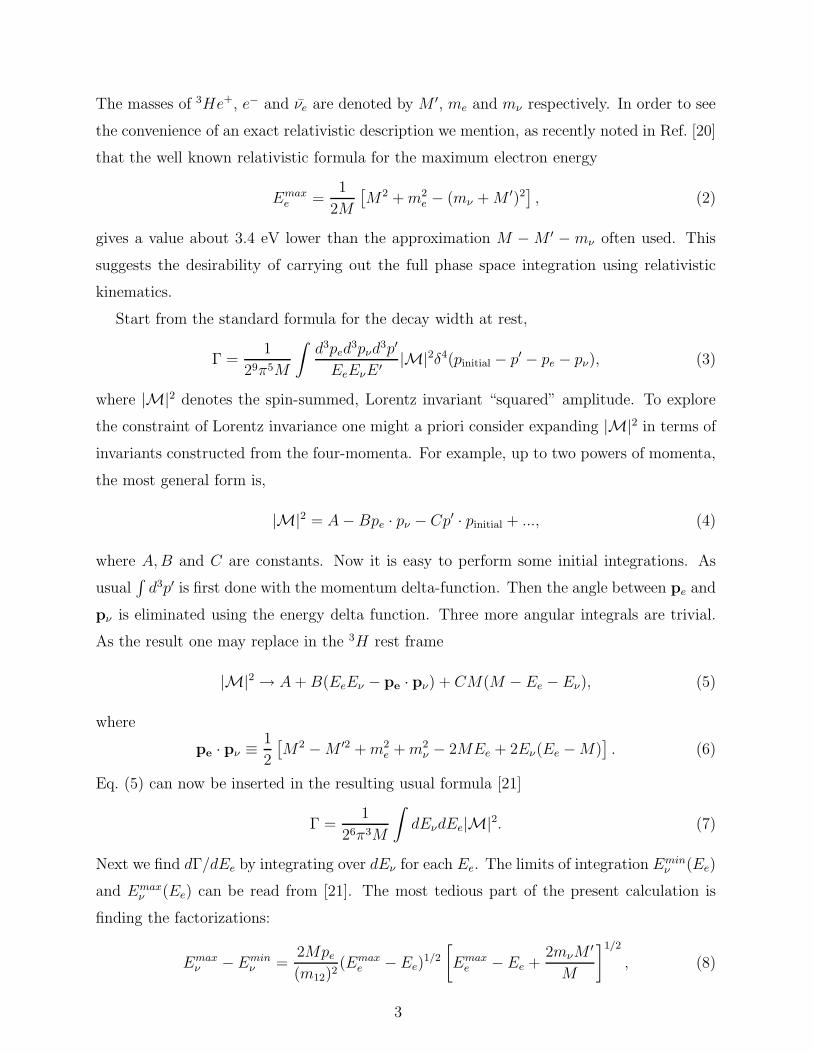
The masses of 3He+, e− and νe are denoted by M ′, me and mν respectively. In order to see

the convenience of an exact relativistic description we mention, as recently noted in Ref. [20]

that the well known relativistic formula for the maximum electron energy

Emaxe =

1

2M

[

M2 + m2e − (mν + M ′)2

]

, (2)

gives a value about 3.4 eV lower than the approximation M − M ′ − mν often used. This

suggests the desirability of carrying out the full phase space integration using relativistic

kinematics.

Start from the standard formula for the decay width at rest,

Γ =1

29π5M

∫

d3ped3pνd

3p′

EeEνE ′|M|2δ4(pinitial − p′ − pe − pν), (3)

where |M|2 denotes the spin-summed, Lorentz invariant “squared” amplitude. To explore

the constraint of Lorentz invariance one might a priori consider expanding |M|2 in terms of

invariants constructed from the four-momenta. For example, up to two powers of momenta,

the most general form is,

|M|2 = A − Bpe · pν − Cp′ · pinitial + ..., (4)

where A, B and C are constants. Now it is easy to perform some initial integrations. As

usual∫

d3p′ is first done with the momentum delta-function. Then the angle between pe and

pν is eliminated using the energy delta function. Three more angular integrals are trivial.

As the result one may replace in the 3H rest frame

|M|2 → A + B(EeEν − pe · pν) + CM(M − Ee − Eν), (5)

where

pe · pν ≡ 1

2

[

M2 − M ′2 + m2e + m2

ν − 2MEe + 2Eν(Ee − M)]

. (6)

Eq. (5) can now be inserted in the resulting usual formula [21]

Γ =1

26π3M

∫

dEνdEe|M|2. (7)

Next we find dΓ/dEe by integrating over dEν for each Ee. The limits of integration Eminν (Ee)

and Emaxν (Ee) can be read from [21]. The most tedious part of the present calculation is

finding the factorizations:

Emaxν − Emin

ν =2Mpe

(m12)2(Emax

e − Ee)1/2

[

Emaxe − Ee +

2mνM′

M

]1/2

, (8)

3

Emaxν + Emin

ν =2M

(m12)2(M − Ee)

[

Emaxe − Ee +

mν

M(M ′ + mν)

]

, (9)

wherein:

(m12)2 = M2 − 2MEe + m2

e. (10)

The importance of the factorization is that it makes the behavior at the endpoint Ee = Emaxe

transparent. Then we have the exact relativistic result,

dΓ

dEe=

1

(2π)3

pe

4(m12)2

√

y

(

y +2mνM ′

M

)

[A + CM(M − Ee) +

+BMMEe − m2

e

(m12)2

(

y +mν

M(M ′ + mν)

)

− CM2

(m12)2(M − Ee)

(

y +mν

M(M ′ + mν)

)

],(11)

where y = Emaxe − Ee.

As it stands, this formula is based only on the kinematical assumption in Eq. (4). It

obviously vanishes at the endpoint y = 0 as√

y. Note that all other terms are finite at

y = 0. The overall factor√

y(y + 2mνM ′/M) gives the behavior of dΓ

dEe

extremely close to

y = 0 for any choice of A, B and C, but departs from dΓ

dEe

away from the endpoint.

Dynamics is traditionally put into the picture [22] by examining the spin sum for a

4-fermion interaction wherein the nuclear matrix element is assumed constant. This is

presented as a non- Lorentz invariant term,

|M|2 = BEeEν . (12)

We will see that this is excellently approximated in our fully relativistic model by,

A = C = 0, B 6= 0. (13)

A more accurate treatment of the underlying interaction might give rise to small admixtures

of non-zero A and C as well as other unwritten coefficients in Eq. (4) above.

The form for the spectrum shape near the endpoint that results from putting A = C = 0

in Eq. (11) is

dΓ

dEe

=peMB

(2π)34(m12)4(MEe − m2

e)

√

y

(

y +2mνM ′

M

)

[

y +mν

M(M ′ + mν)

]

. (14)

Note that if we had employed the non-relativistic form given in Eq. (12) the net result would

be a replacement of an overall factor in Eq. (14) according to,

(MEe − m2e) → (MEe − E2

e ). (15)

4

The difference of these two factors yields the contribution of the pe · pν term. It is really

negligible near the endpoint region since it is proportional to p2e and is suppressed like

p2e/(MEe) compared to unity. We have checked that the result of our calculation with just

the EeEν term agrees with the calculation of Ref. [23], though their result looks much more

complicated, as they did not present it in the simpler factorized form given here.

Note that only the two rightmost factors vary appreciably near the endpoint of Eq. (14).

If we further approximate M ′/M → 1 and M ′+mν

M→ 1 the endpoint shape is well described

bydΓ

dEe

α (y + mν)√

y(y + 2mν). (16)

Now we compare with the formula used in the experimental analysis [15]

dΓ

dEeα (E0 − Vi − E)

√

(E0 − Vi − E)2 − m2ν . (17)

This agrees with the above approximation in Eq. (16) if one identifies

(E0 − Vi − E) = y + mν . (18)

Note that E is the non-relativistic energy given by E = Ee − me. Furthermore, E0 − Vi is

identified with our (M − M ′ − me − δEmaxe ). δEmax

e is defined by,

Emaxe = M − M ′ − mν − δEmax

e , (19)

and was shown in [20] to be independent of mν to a good approximation. Thus we see that

the exact relativistic endpoint structure obtained here may be well approximated by the

form used in the experimental analysis.

Often, authors express results in terms of a variable, x, which from our discussion may

be seen to be the same as,

x = −y − mν = Ee − Emaxe − mν . (20)

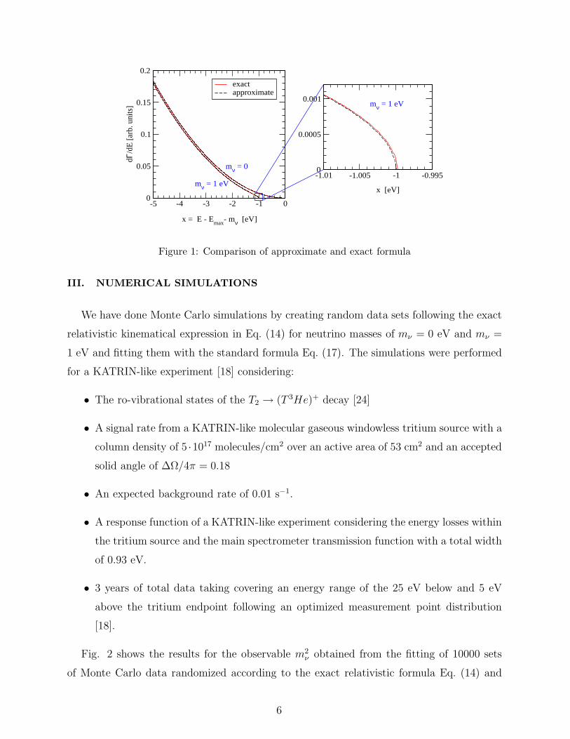
In Fig. 1, dΓ/dEe as computed from the exact formula, Eq. (14) is compared with its approx-

imate analog as a function of x. As can be seen, the differences between the approximate

and exact formulae are tiny.

It may be worthwhile to remark that the exact relativistic kinematical expression in

Eq. (14) is no more complicated than the approximation one ordinarily uses.

5

-5 -4 -3 -2 -1 0

x = E - Emax

- mν [eV]

0

0.05

0.1

0.15

0.2

dΓ/d

E [

arb.

uni

ts]

exactapproximate

-1.01 -1.005 -1 -0.9950

0.0005

0.001

mν = 0

mν = 1 eV

mν = 1 eV

x [eV]

Figure 1: Comparison of approximate and exact formula

III. NUMERICAL SIMULATIONS

We have done Monte Carlo simulations by creating random data sets following the exact

relativistic kinematical expression in Eq. (14) for neutrino masses of mν = 0 eV and mν =

1 eV and fitting them with the standard formula Eq. (17). The simulations were performed

for a KATRIN-like experiment [18] considering:

• The ro-vibrational states of the T2 → (T 3He)+ decay [24]

• A signal rate from a KATRIN-like molecular gaseous windowless tritium source with a

column density of 5 ·1017 molecules/cm2 over an active area of 53 cm2 and an accepted

solid angle of ∆Ω/4π = 0.18

• An expected background rate of 0.01 s−1.

• A response function of a KATRIN-like experiment considering the energy losses within

the tritium source and the main spectrometer transmission function with a total width

of 0.93 eV.

• 3 years of total data taking covering an energy range of the 25 eV below and 5 eV

above the tritium endpoint following an optimized measurement point distribution

[18].

Fig. 2 shows the results for the observable m2ν obtained from the fitting of 10000 sets

of Monte Carlo data randomized according to the exact relativistic formula Eq. (14) and

6

Figure 2: Results on the observable m2ν from the fitting of 10000 sets of Monte Carlo data ran-

domized according to the exact relativistic formula Eq. (14) and to a fitting routine based on the

standard formula Eq. (17), for neutrino masses of 0 eV (left) and 1 eV (right). The rms values

of the Gaussian-like distributions correspond to the expected statistical uncertainty ∆m2ν,stat for a

KATRIN-like experiment.

to a fitting routine using the standard formula Eq. (17), assuming neutrino masses of 0 eV

(left) and 1 eV (right). The rms values of the Gaussian-like distributions correspond to

the expected statistical uncertainty ∆m2ν,stat for a KATRIN-like experiment. Clearly the

mean value of the fit results for the neutrino mass squared m2ν does not show any significant

deviation from the starting assumption of mν = 0 eV or mν = 1 eV, respectively. This

establishes that the exact relativistic formula Eq. (14) can be well approximated by the

standard equation (17) for the precision needed for the next generation tritium experiment

KATRIN. This is probably due to the fact that KATRIN is investigating the last 25 eV

below of the beta spectrum below its endpoint only, where the recoil corrections are nearly

independent on the electron energy.

7

IV. THREE NEUTRINO CASE

Of course, the most interesting application is to the case of three neutrinos with different

masses, m1, m2 and m3. Then there will be a different endpoint energy, Emaxi corresponding

to each one. The effective endpoint factor in the good approximation of Eq. (16) is the

weighted sum,

Feff (Ee) =3

∑

i=1

|K1i|2(yi + mi)[yi(yi + 2mi)]1/2θ(yi), (21)

where yi(Ee) = Emaxi −Ee and the K1i are the elements of the 3x3 lepton mixing matrix [25,

26]. We note that the further good approximation that the quantity δEmaxe is independent

of the neutrino mass, gives the useful relation

yi − yj = mj − mi. (22)

Now let the unindexed quantity y stand for the yi with the smallest of the neutrino masses.

Using Eq. (22) allows us to write the explicit formula for the case (denoted “normal hierar-

chy”) where m1 is the lightest of the three neutrino masses as:

FNH(y) = |K11|2(y + m1)[y(y + 2m1)]1/2 (23)

+ |K12|2(y + m1)[(y + m1 − m2)(y + m1 + m2)]1/2θ(y + m1 − m2)

+ |K13|2(y + m1)[(y + m1 − m3)(y + m1 + m3)]1/2θ(y + m1 − m3).

In the other case of interest (denoted “inverse hierarchy”) we have:

FIH(y) = |K13|2(y + m3)[y(y + 2m3)]1/2 (24)

+ |K11|2(y + m3)[(y + m3 − m1)(y + m3 + m1)]1/2θ(y + m3 − m1)

+ |K12|2(y + m3)[(y + m3 − m2)(y + m3 + m2)]1/2θ(y + m3 − m2).

where m3 is the lightest of the three neutrino masses. From these equations we may easily

find the counting rate in the energy range from the appropriate endpoint up to ymax as

proportional to the integral

nNH(ymax) =

∫ ymax

0

dyFNH(y), (25)

or, for the “inverse hierarchy” case, as proportional to,

nIH(ymax) =

∫ ymax

0

dyFIH(y). (26)

8

We note that, as stressed in ref. [20], information on neutrino masses and mixings ob-

tained from neutrino oscillation experiments is actually sufficient in principle to predict

n(ymax) as a function of a single parameter (up to a twofold ambiguity). Thus, in princi-

ple, suitably comparing the predicted values of n(ymax) with results from a future endpoint

experiment may end up determining three neutrino masses.

To see how this might work out we make an initial estimate using the best fit values [6]

of neutrino squared mass differences,

A ≡ m22 − m2

1 = 7.9 × 10−5eV 2, (27)

B ≡ |m23 − m2

2| = 2.6 × 10−3eV 2,

and the weighting coefficients,

|K11|2 = 0.67, (28)

|K12|2 = 0.29,

|K13|2 = 0.04.

Currently |K13|2 is consistent with zero and is only bounded. For definiteness we have

taken a value close to the present upper bound. However, we have checked that the effect

of putting it to zero is very small. Now, from the two known differences in Eq. (27) we

can for each choice of m3 (considered as our free parameter) find the masses m1 and m2,

subject to the ambiguity as to whether m3 is the largest (NH) or the smallest (IH) of the

three neutrino masses. Of course we hope that future long baseline neutrino oscillation

experiments [27, 28, 29, 30] might eventually determine whether nature prefers the NH or

the IH scenario.

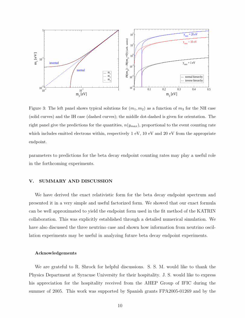
Fig. 3 shows typical solutions for the mass set (m1, m2) in terms of the free parameter

m3. Very large values of m3 would fall within the sensitivity of upcoming cosmological

tests [10, 11]. In the right panel of Fig. 3 we display the predicted values of n(ymax) for

each possible mass scenario and the choices of (1,10,20) eV for ymax. These quantities are

proportional to the electron counting rate in the energy interval from the endpoint (for

each mass scenario) to ymax eV below the endpoint. The different values of ymax reflect,

of course, different experimental sensitivities. The main point is that, for sufficiently large

m3 values, the counting rate is seen to distinguish the different possible neutrino mass sets

from each other. We hope that the present method of relating observed neutrino oscillation

9

10-2

10-1 1

m3 [eV]

10-2

10-1

1

mi [

eV]

m1

m2

m3

normal

inverted

0 0.1 0.2 0.3 0.4 0.5

m3 [eV]

10-3

10-2

10-1

100

101

102

n(m

3)

- n

(m3=

0)

[arb

. u

nit

s]

normal hierarchyinverse hierarchy

ymax

= 1 eV

ymax

= 10 eV

ymax

= 20 eV

Figure 3: The left panel shows typical solutions for (m1,m2) as a function of m3 for the NH case

(solid curves) and the IH case (dashed curves); the middle dot-dashed is given for orientation. The

right panel give the predictions for the quantities, n(ymax), proportional to the event counting rate

which includes emitted electrons within, respectively 1 eV, 10 eV and 20 eV from the appropriate

endpoint.

parameters to predictions for the beta decay endpoint counting rates may play a useful role

in the forthcoming experiments.

V. SUMMARY AND DISCUSSION

We have derived the exact relativistic form for the beta decay endpoint spectrum and

presented it in a very simple and useful factorized form. We showed that our exact formula

can be well approximated to yield the endpoint form used in the fit method of the KATRIN

collaboration. This was explicitly established through a detailed numerical simulation. We

have also discussed the three neutrino case and shown how information from neutrino oscil-

lation experiments may be useful in analyzing future beta decay endpoint experiments.

Acknowledgements

We are grateful to R. Shrock for helpful discussions. S. S. M. would like to thank the

Physics Department at Syracuse University for their hospitality. J. S. would like to express

his appreciation for the hospitality received from the AHEP Group of IFIC during the

summer of 2005. This work was supported by Spanish grants FPA2005-01269 and by the

10

EC RTN network MRTN-CT-2004-503369. The work of J.S. is supported in part by the

U.S. DOE under Contract no. DE-FG-02-85ER 40231. S.N. was supported by the DOE

Grant DE-FG02-97ER41029.

[1] Super-Kamiokande collaboration, S. Fukuda et al., Phys. Lett. B539, 179 (2002),

[hep-ex/0205075].

[2] SNO collaboration, Q. R. Ahmad et al., Phys. Rev. Lett. 89, 011301 (2002), [nucl-ex/0204008].

[3] KamLAND collaboration, T. Araki et al., Phys. Rev. Lett. 94, 081801 (2004).

[4] For a review see T. Kajita, New J. Phys. 6, 194 (2004).

[5] K2K collaboration, M. H. Ahn et al., Phys. Rev. Lett. 90, 041801 (2003), [hep-ex/0212007].

[6] For an uptaded review see M. Maltoni, T. Schwetz, M. A. Tortola and J. W. F. Valle, New

J. Phys. 6, 122 (2004), hep-ph/0405172 (v5); previous works by other groups are referenced

therein.

[7] WMAP collaboration, D. N. Spergel et al., astro-ph/0603449.

[8] M. Colless et al., Mon. Not. R. Astron. Soc 328, 1039 (2001).

[9] SDSS collaboration, M. Tegmark et al., Phys. Rev. D 69, 103501 (2004), [astro-ph/0310723].

[10] J. Lesgourgues and S. Pastor, Phys. Rep. 429, 307 (2006), [astro-ph/0603494].

[11] S. Hannestad, Ann. Rev. Nucl. Part. Sci. 56, 137 (2006), [hep-ph/0602058].

[12] S. R. Elliott and P. Vogel, Ann. Rev. Nucl. Part. Sci. 52, 115 (2002), [hep-ph/0202264].

[13] KATRIN collaboration, A. Osipowicz et al., hep-ex/0109033.

[14] V. M. Lobashev, Nucl. Phys. A719, 153 (2003).

[15] C. Kraus et al., Eur. Phys. J. C40, 447 (2005), [hep-ex/0412056].

[16] G. Drexlin for the KATRIN collaboration, Nucl. Phys. Proc. Suppl. 145, 263 (2005).

[17] C. Weinheimer, Nucl. Phys. Proc. Suppl. 168, 5 (2007)

[18] KATRIN collaboration, J. Angrik et al., FZKA-7090 (KATRIN design report 2004).

[19] A. Monfardini et al., Prog. Part. Nucl. Phys. 57, 68 (2006), [hep-ex/0509038].

[20] S. S. Masood, S. Nasri and J. Schechter, Int. J. Mod. Phys. A21, 517 (2006), [hep-ph/0505183].

[21] Particle Data Group, S. Eidelman et al., Phys. Lett. B592, 1 (2004).

[22] J. D. Bjorken and S. D. Drell, Relativistic Quantum Mechanics (McGraw-Hill, N.Y., 1964).

[23] C.-E. Wu and W. W. Repko, Phys. Rev. C27, 1754 (1983).

[24] A. Saenz, S. Jonsell and P. Froelich, Phys. Rev. Lett. 84, 242 (2000).

11

[25] J. Schechter and J. W. F. Valle, Phys. Rev. D22, 2227 (1980).

[26] Particle Data Group, W. M. Yao et al., J. Phys. G33, 1 (2006).

[27] C. Albright et al., hep-ex/0008064, Report to the Fermilab Directorate.

[28] M. Apollonio et al., hep-ph/0210192, CERN Yellow Report on the Neutrino Factory.

[29] P. Huber, M. Lindner and W. Winter, Nucl. Phys. B645, 3 (2002), [hep-ph/0204352].

[30] Muon Collider/Neutrino Factory, M. M. Alsharoa et al., Phys. Rev. ST Accel. Beams 6,

081001 (2003), [hep-ex/0207031].

12