Relativistic Methods for Calculating Electron Paramagnetic ...

HAL Id: hal-02483183https://hal.archives-ouvertes.fr/hal-02483183

Submitted on 18 Feb 2020

HAL is a multi-disciplinary open accessarchive for the deposit and dissemination of sci-entific research documents, whether they are pub-lished or not. The documents may come fromteaching and research institutions in France orabroad, or from public or private research centers.

L’archive ouverte pluridisciplinaire HAL, estdestinée au dépôt et à la diffusion de documentsscientifiques de niveau recherche, publiés ou non,émanant des établissements d’enseignement et derecherche français ou étrangers, des laboratoirespublics ou privés.

Relativistic Methods for Calculating ElectronParamagnetic Resonance (EPR) Parameters

Hélène Bolvin, Jochen Autschbach

To cite this version:Hélène Bolvin, Jochen Autschbach. Relativistic Methods for Calculating Electron Paramagnetic Res-onance (EPR) Parameters. Springer. Handbook of Relativistic Quantum Chemistry, Springer BerlinHeidelberg, pp.1-39, 2015, �10.1007/978-3-642-41611-8_12-1�. �hal-02483183�

https://hal.archives-ouvertes.fr/hal-02483183

https://hal.archives-ouvertes.fr

Chapter 0Relativistic methods for calculating ElectronParamagnetic Resonance (EPR) parameters

Helene Bolvin and Jochen Autschbach

Abstract Basic concepts for calculating electronic paramagnetic resonance are dis-cussed, with a focus on methods that are suitable for molecules containing heavyelements. Inclusion of relativistic effects is essential in such calculations. Selectedexamples are presented to illustrate practical applications of these theoretical meth-ods

Preliminaries: Units, Notation, Acronyms

The reader is assumed to be familiar with basic concepts of quantum mechanics– including relativistic methods covered in other chapters – and basic concepts ofcomputational chemistry. SI units are employed. Nuclear motion is not considered;the focus is on electronic structure and the resulting magnetic properties. The sym-bols · and× indicate inner and outer products, respectively, for vectors and matricesor tensors. Bold-italic notation such as r, S,µ is used for vectors and vector opera-tors, while upright-bold such as a,G,µ is used for matrices and rank-2 tensors.

The following acronyms are used occasionally in the text:

AO atomic orbital (basis function or actual AO)CAS complete active spaceDFT Density Functional Theory (usually KS, ‘pure’ and generalized KS variants)EM electro-magneticGIAO gauge-including atomic orbitalHF Hartree-FockHFC hyperfine coupling

Please address correspondence to either one of the authors. Helene Bolvin, Laboratoire de Physiqueet de Chimie Quantiques, Universite Toulouse 3, 118 Route de Narbonne, 31062 Toulouse, France,e-mail: [email protected]. Jochen Autschbach, Department of Chemistry, Uni-versity at Buffalo, State University of New York, e-mail: [email protected]

1

2 Helene Bolvin and Jochen Autschbach

KS Kohn-ShamMO molecular orbitalNR non-relativistic (calculation excluding any relativistic effects)PV principal value (of a tensor)PAS principal axis system (of a tensor)QM quantum mechanical (e.g. in reference to Dirac, Schrodinger Eqs.)SO spin-orbit (usually means calculation also includes SR effects)SOS sum over statesSR scalar relativistic (relativistic calculation without SO effects)WFT wave-function theoryZFS zero-field splitting

0.1 Introduction and Background: EPR parameters and SpinHamiltonians

Many of the chemical species encountered in the laboratory and in everyday lifehave non-degenerate closed shell ground states. But there are also many exceptions,such as open shell metal complexes, stable radicals, and most atoms. In the absenceof external electromagnetic (EM) fields, such species may afford a degenerate elec-tronic ground state and degenerate excited states. Species with closed-shell groundstates may also afford degenerate excited states such as excited spin triplets. Theterm degeneracy means that an electronic state λ with energy Eλ may have dλ statecomponents |λ, a〉, with a = 1 . . . dλ, such that each |λ, a〉 and any linear com-bination thereof is a solution to the field-free quantum mechanical (QM) equationdescribing the system (e.g. Schrodinger equation, Dirac equation, approximate two-component relativistic QM methods, as discussed elsewhere in this Handbook) withthe same energy Eλ. The index λ may simply be a number counting the energylevels of the system, or it may be a spectroscopic symbol characterizing a state ofinterest, or a symmetry label, or a combination thereof. The discussion excludescases of accidental degeneracy.

Electron paramagnetic resonance (EPR) [1–4] is a primary tool for studying de-generate and nearly degenerate electronic states experimentally. An external mag-netic field B splits the degeneracy (Zeeman effect) to yield a new set of states. EMradiation of a suitable frequency may then induce transitions among them and allowto measure the energy splittings spectroscopically. The parameters extracted fromthe spectra (vide infra) contain a wealth of information about the electronic structureand molecular structure.

To illustrate the effect utilized in EPR spectroscopy, consider a single unpairedelectron and – first – neglect spin-orbit (SO) coupling. This situation represents aspin doublet (a two-fold degenerate state) with spin quantum number S = 1/2. Ifthere is no external magnetic field, the two possible orientations of the spin projec-tion onto a quantization axis (MS = ±1/2) have the same energy. Associated withthe spin angular momentum vector S is a magnetic dipole moment µe = −geβeS,

0 Electron Paramagnetic Resonance Parameters 3

with βe = eh/(2me) being the Bohr magneton and ge the free electron g-value or g-factor with a current experimental value [5] of 2.002 319 304 361 53 (53). The Diracequation predicts ge = 2 exactly. Therefore, ge = 2 is used occasionally in the fol-lowing. The small differences in the values of ge are due to quantum electrodynamiccorrections.

For S = 1/2 the magnetic moment associated with the spin has two projectionsonto a quantization axis. If a static external magnetic field is applied, the directionof B defines the quantization axis. With the field present, the quantized projectionsof µe do not have the same energy. In classical physics, the energy of a magneticdipole µ in a magnetic fieldB is

E = −µ ·B (0.1)

The lowest energy is for µ andB being anti-parallel, and the highest energy is for µand B being parallel. This is the physical mechanism that keeps a compass needlepointing toward the magnetic north pole. Quantum mechanically, a semi-classicalZeeman Hamiltonian that describes such an effect for a quantized spin magneticmoment is

HZ = geβeS ·B (0.2)

with S being the spin vector operator. The negative sign in (0.1) is canceled by thenegative sign relating µe to the spin. One may choose a coordinate system such thatB is oriented along the z axis, with amplitudeB0. The Hamiltonian (0.2) then reads

HZ = geβeB0Sz (0.3)

The eigenvalues are those of Sz times geβeB0, i.e. ±(1/2)geβeB0. The magneticfield lifts the degeneracy of the spin doublet. A transition from the lower energylevel (B and S ‘anti-parallel’) to the higher one (B and S ‘parallel’) requires anenergy of

∆E = hν = geβeB0 (0.4)

In the equation above, ν is the frequency of EM radiation used to induce the tran-sition. The frequency is approximately 28 GHz / T. In a typical EPR spectrometer,B0 is 0.34 T (3,400 Gauss), which translates to a free electron spin-1/2 resonancefrequency of about 9.5 GHz. This is radiation in the X-band microwave region ofthe EM spectrum. For general spin values S, the degeneracy of the projection is2S + 1. A magnetic field splits these into 2S + 1 individual states. Absorption of aphoton of EM radiation entails conservation of angular momentum. The photon hasan angular momentum of h, corresponding to one atomic unit (au), and thereforethe selection rule is that transitions with ∆MS = 1 are allowed.

One may repeat the calculation for the spin IK of some nucleus no.K, by substi-tuting the electron spin magnetic dipole moment by the nuclear spin magnetic dipolemoment µK = gKβNIK . Here, gK is the g-factor for a given nuclear isotope, andβN = eh/(2MP ) is the nuclear magneton, with MP being the proton mass. Thelatter is approximately 2000 times greater than the electron mass, and thereforethe associated transition energies for nuclear spins are in the radio-frequency range


(tens of MHz) at magnetic field strengths used in EPR spectrometers. Transitionsbetween nuclear spin projections are observed directly in nuclear magnetic reso-nance (NMR). At EPR spectrometer field strengths, the energy splitting for nucleartransitions is very small and one may assume equal Boltzmann populations of thenuclear spin projection states in the absence of other magnetic fields. However, thereis a magnetic coupling of electronic and nuclear magnetic moments called hyperfinecoupling (HFC). Hyperfine coupling gives rise to hyperfine structure of EPR spectrawhen nuclei with non-zero spin are present.

There is another type of fine structure that can be observed in EPR experimentsfor systems with S ≥ 1. For a given magnetic field strength B0, the 2S + 1 spinprojections with differentMS would be expected to be equally spaced energetically,meaning that any of the possible 2S allowed transitions with ∆MS = 1 give res-onances at the same frequency. However, at lower field strengths the spectra mayexhibit 2S distinct features at lower field strengths [1], which indicates unequal en-ergetic separations of the MS components in the presence of the field. This finestructure can be traced back to a removal of the degeneracy of the spin multipletalready at zero field. The effect is therefore called zero field splitting (ZFS). A spinS ≥ 1 implies that there are two or more unpaired electrons. The physical originof ZFS is a magnetic interaction between pairs of electrons, either directly (a dipo-lar spin-spin interaction arising from relativistic corrections to the electron-electroninteraction) or mediated via SO coupling (which has one- and two-electron contri-butions). The ZFS can therefore be associated with relativistic effects. For systemswith heavy elements, as well as for many lighter systems, the SO contribution toZFS is the dominant one.

The observed electronic magnetic moment resulting from an electronically de-generate state may differ from what is expected based solely on the spin quantumnumber. For instance there may be an orbital degeneracy present in an electronicstate, meaning that the observed magnetic moment is not only due to an electronspin but also due to an orbital angular momentum. The interaction with the externalfield can be expressed via the total angular momentum J , which is obtained fromthe vector addition of the quantized spin and orbital angular momenta, S and L. Asan example, the S = 1/2, L = 1 (2P ) ground state of the fluorine atom has a totalangular momentum quantum number J = 3/2, with total spin and orbital angularmomentum parallel, giving a 4-fold degenerate state (MJ ranging from +3/2 to−3/2) whose components split in the presence of a magnetic field. Transitions inthe EPR experiment may be observed for ∆MJ = 1. Instead of Equation (0.4), thetransition frequencies are determined by

∆E = hν = gJβeB0 (0.5)

with gJ = 4/3 for the fluorine 2P3/2 state, instead of 2. Here, gJ is the Lande g-factor; the experimentally observed g-factor obtained from matching the measuredresonance frequency with Equation (0.5) for known field strengthB0 is very close tothis number. The large difference of gJ from the free-electron ge = 2 arises becausethe state reflects not only a spin doublet but also an orbital triplet.


In the absence of orbital degeneracy, an orbital magnetic moment and deviationsof observed g-factors from the free electron value may arise because of SO coupling.For organic doublet radicals with only light elements, S = 1/2,MS = ±1/2 arebasically good quantum numbers. However, even in this situation the observed g-factors may differ from 2 (typically ranging from 1.9 to 2.1) because of SO coupling.Because of the small deviations, it is sometimes preferred to report g-shifts ∆g =g−ge (often in units of parts per thousand (ppt)), in analogy to NMR chemical shifts.Since SO coupling is a relativistic effect, the presence of g-shifts for orbitally non-degenerate states directly indicates relativistic effects. If SO coupling is strong, Sand MS may not be good quantum numbers at all. In this case, g-shifts can becomevery large even in the absence of orbital degeneracy (meaning an absence of orbitalangular momentum in the corresponding scalar relativistic (SR) state). A case inpoint is the doublet ground state of NpF6 for which the observed [6] g-factor is−0.6.

To summarize: A degenerate paramagnetic electronic state gives rise to a moreor less complicated pattern of EPR resonances. Given the potential influence of SOcoupling, orbital angular momenta, and ZFS, the spectrum is usually interpretedand quantified by invoking the concept of a pseudo-spin S rather than the actualelectron spin S. The value of S defines the degeneracy, 2S + 1, of the state that issplit by the magnetic field into components with different MS . The various effectsdiscussed above can be included in a phenomenological pseudo-spin Hamiltonian,which, in lowest order, reads

HS = βeB · g · S + IK · aK · S + S · d · S (0.6)

The parameters in the Hamiltonian are determined by requiring that the transitionswith ∆MS = 1 between its eigenstates reproduce the observed spectrum. Thespin Hamiltonian is designed such that its elements within the set of fictitious spineigenstates are the same as the matrix elements of the true Hamiltonian within theset of true eigenstates. It supposes a correspondence between pseudo-spin and trueeigenstates, up to a phase factor common to all the vectors. While this assignmentcan be rather arbitrary, the basic requirement is that the spin Hamiltonian in thefictitious space transforms in coherence as the real Hamiltonian does in the realspace, either by time inversion or by the spatial symmetries of the molecule. [7]

On the right-hand side of Equation (0.6) are, from left to right, the pseudo-spinoperators for the Zeeman interaction, the HFC interaction, and the ZFS. Only thepseudo-spin related to the electronic state is treated quantum mechanically. Thenuclear spin and external magnetic field are parameters. In Equation (0.6), g, aK ,and d are 3 × 3 matrices parametrizing the various interactions. The fact that theyare written in matrix form reflects the possibility that the observed interactions maybe anisotropic. For example, observed g-factors for a molecule with axial symmetrymay be very different if the magnetic field is oriented along the axial direction orperpendicular to it. Higher order terms requiring additional sets of parameters inEquation (0.6) may be required to reflect the full complexity of an EPR spectrum,as discussed in Section 0.3.


The matrices g and aK are often referred to as the g-‘tensor’ and the HFC ‘ten-sor’. It was pointed out in the book by Abragam & Bleaney [4] that they are infact not proper rank-2 tensors. Following a suggestion by Atherton [1], one mayrefer to them as the Zeeman coupling matrix (g) and the HFC matrix (aK) instead.The g-factor observed for a magnetic field in the direction of a unit vector u in thelaboratory coordinate system is given by

gu = ±(u · ggT · u)1/2 (0.7)

(superscript T indicating a matrix transpose). One may define a hyperfine couplingassociated with a particular quantization direction chosen for the pseudo-spin in asimilar way. The corresponding objects G = ggT and AK = aKaTK are rank-2tensors whose eigenvalues and eigenvectors define the squares of the principal val-ues (PVs) of g and aK and a principal axis system (PAS) of each of the interactions.For example, the principal g-factors correspond to the g-factors that are observedwhen the direction of the magnetic fieldB coincides with one of the principal axes.Section 0.4 addresses the question of the signs of the PVs of the Zeeman and HFCinteraction in more detail.

Section 0.2 sketches different computational relativistic methods by which toobtain the EPR parameters in the spin Hamiltonian of Equation (0.6) from first prin-ciples. As already mentioned, SO coupling plays an important role. HFC can also bestrongly impacted by SR and SO relativistic effects. Selected illustrative examplesare presented in Section 0.5.

0.2 Computational methods for EPR parameter calculations

0.2.1 Representation of the pseudo-spin Hamiltonian in anab-initio framework

Equation (0.6) and generalizations thereof presents some conceptual challengeswhen addressing the problem by relativistic or non-relativistic (NR) molecular quan-tum mechanics. The reason is that the pseudo-spin operator S may have little incommon with the electron spin operator S if SO coupling or ZFS are strong, or ifthe orbital angular momenta are not quenched. What can be done instead followsroughly the following sequence [3], if a calculation starts out with a pure spin-multiplet (i.e. from a NR or SR reference without orbital degeneracy) and if effectsfrom SO coupling can be dealt with as a perturbation:

• Define a Hamiltonian H0 for the system in the absence of external EM fields andfind its eigenstates with energies Eλ, spin degeneracies dλ, and correspondingorthonormal QM eigenfunctions |λ, a〉.

• Consider a perturbation: a homogeneous external fieldB for the Zeeman interac-tion, the hyperfine magnetic field from a nuclear spin magnetic moment µK , or


spin-dependent perturbations. Define a corresponding perturbation HamiltonianH′. The effects from SO coupling may also be absorbed into H′. The perturba-tions are assumed to be weak enough such that one can identify the eigenstatesof H0 + H′ corresponding to a multiplet λ of H0 of interest. Diagonalization ofthe matrix H0 + H′ representing the Hamiltonian in the complete set (or a largesubset) of eigenstates of H0, or finding a selected number of eigenfunctions andeigenvalues with techniques such as the Davidson or Lanczos algorithms, wouldgive the eigenfunctions and energies for the perturbed system. Typically, therewould be a mixing among eigenvectors belonging to a multiplet λ as well assome admixture from components of other multiplets.

• Instead, select a multiplet λ with degeneracy dλ of interest corresponding to H0,and seek a dλ × dλ matrix representation Heff of an effective Hamiltonian Heffwith the following properties: (i) the eigenvalues of Heff are the same as thoseof H0 + H′ for the perturbed multiplet λ. (ii) The eigenvectors of Heff describehow the components of the unperturbed multiplet mix under the perturbation.There are various ways by which Heff can be calculated. A well-known approachis by perturbation theory as an approximation to second order, which gives for amatrix element related to the multiplet λ:

〈λa|Heff|λa′〉 = δaa′Eλ + 〈λa|H(a)|λa′〉−∑µ6=λ

dµ∑b=1

〈λa|H(b)|µb〉〈µb|H(c)|λa〉Eλ − Eµ

(0.8)Here, H(a), H(b), and H(b) are parts of H′ such that the overall matrix element(minus the δaa′Eλ part) affords terms that are linear in B or IK , or bi-linear inelectron spin operators.

• Apart from a constant shift on the diagonal, the matrix representation of thepseudo-spin Hamiltonian, Equation (0.6), written in terms of |MS 〉 pseudo-spinprojects is then supposed to have the same elements as those of Heff. For theZeeman interaction, the contribution to Heff should be linear in B. Then, H(a)

and H(b) are the Zeeman operator (in a suitable relativistic form) and H(c) addi-tionally considers SO effects. If H(a) and H(b) are instead QM operators linearin IK describing the nuclear hyperfine field, a mapping onto the HFC part of thepseudo-spin Hamiltonian can be made. Finally, if H(a) is the dipolar spin-spininteraction operator, and H(b) and H(c) represent SO interactions, one obtains aneffective Hamiltonian quadratic in the electron spin which represents ZFS.

In the previous approach, the matching between real and fictitious states is madeaccording to |λ,M〉 ≡ |S ,MS 〉 since the model space is a spin multiplet; it sup-poses a similarity between the real spin and the pseudo-spin. This is only valid inthe weak SO limit but the procedure permits the calculation of the spin Hamiltonianparameters for all values of the pseudo-spin S [8]. Equation (0.8) misses quadraticcontributions which may be important [9].

The value of the pseudo-spin S defines the size of the model space. If the stateof interest, usually the ground state, is d-fold degenerate or nearly degenerate, Sis chosen such that d = 2S + 1. In the case of weak SO coupling and a spatially


non degenerate state 2S+1Γ where Γ is a non degenerate irreducible representation(irrep) of the system’s point group, the SO coupling with the excited states splits thespin degeneracy. This ZFS splitting is on the order of a few cm−1 and gives the finestructure to the EPR spectra. In some cases, the ZFS splitting may be on the orderof several ten cm−1 and high-field high-frequency EPR (HF-HF EPR) is necessaryto detect the transitions between these components. In this case, one usually takesS = S. When the ground state is spatially degenerate or if there are very low lyingexcited states, there are large orbital contributions to the magnetic moment and thechoice of the spin Hamiltonian becomes more complicated and must be treated caseby case.

For systems where SO coupling is strong, a close correspondence of a degenerateelectronic state of interest with an electron spin multiplet may simply not exist.A corresponding QM method used to determine the electronic states may alreadyinclude SO coupling in some form, possibly along with a spin-spin interaction term.In this case, the ZFS effects are included in the electronic spectrum. It is shown nexthow the pseudo-spin Hamiltonian parameters for the Zeeman and HFC interactionscan be extracted from such QM calculations. For further discussion see Section 0.3.

When the SO coupling is large, the degeneracy of the states is related to sym-metry. For odd-electron systems, the degeneracy is even due to Kramers’ theorem.Four-fold degenerate irreps only appear in the cubic and icosahedral groups, alongwith six-fold in the latter. Therefore, except for highly symmetric molecules, theground-state of Kramers systems is modeled using S = 1/2. For even-electronsystems, if there is a high-order rotation axis, states may be doubly degenerate andS = 1/2 represents a non-Kramers doublet. Only cubic and icosahedral groupsmay have higher degeneracies. Therefore, the states of even-electron systems with aheavy elements are usually non-degenerate or in the case of symmetry, can be con-sidered as non-Kramers doublets. In lanthanide and actinide complexes, the termof the free ion 2S+1LJ is split due to the environment of the ligands. This splittingis usually on the order of some tens of cm−1 for lanthanides since the 4f orbitalsare mostly inner-shell and interact weakly with the environment. The splitting ofthe free ion term of an actinide is larger since the 5f orbitals interact more withthe ligands, even forming covalent bonds for the early actinides; it can be on theorder of several hundred cm−1. Therefore, in the case of heavy elements, states areat the most doubly degenerate or nearly degenerate and there are usually no EPRtransitions with excited states, except for cubic systems.

An ab-initio calculation provides the 2S + 1 quasi-degenerate wave functions|λ, a〉a=1,2S+1 in the absence of external magnetic field, defining the model space,and the corresponding energies Ea. Let

HZ = −βeµ ·B (0.9)

be the Zeeman operator, with µ being a corresponding dimensionless time-oddQM magnetic moment operator. The Zeeman interaction is characterized by thethree matrices of the magnetization operator (µu)a,b = 〈λ, a|µu|λ, b〉 with a, b ∈[1, 2S + 1] and u = x, y, z being defined in the physical space. Hyperfine matrices


can be defined analogously. These matrices are further discussed in Sections 0.3 and0.4.

The approach is outlined in this section for the Zeeman interaction and a dou-blet of Kramers states (S = 1/2). In this case, there is no ZFS and the spinHamiltonian reduces to the Zeeman term. In the basis of the pseudo-spin projec-tion eigenfunctions |MS 〉, the operator Sk (k = x, y, z) is represented by a matrixSk = (1/2)σk, with σk being one of the 2 × 2 Pauli spin matrices. The magneticfield vector is expressed in terms of its components as B = (B1, B2, B3). Thematrix representation of the spin Hamiltonian for the Zeeman interaction then reads

H =∑k

hkSk with hk = βe∑l

Blglk (0.10)

The eigenvalues are easily obtained as ± the square roots of the eigenvalues of H2,which is already diagonal because of SkSl + SlSk = (δkl/2) ( 1 0

0 1 ):

H2 =1

4

(∑k h

2k 0

0∑k h

2k

)(0.11)

Therefore, the energy difference ∆E for the two spin projections is2[(1/4)

∑k h

2k]1/2 = [

∑k h

2k]1/2, i.e.

∆E = βe

[∑k,l

BkBl∑m

gkmglm

]1/2= βe

[∑k,l

BkBlGkl

]1/2(0.12)

In the previous equation, Gkl is an element of the tensor G introduced below Equa-tion (0.7).

Next, consider a quantum mechanical framework with a doublet state with twowavefunction components,ψ1, ψ2, assumed to be orthonormal for convenience. Fur-ther, for the time being it is assumed that the doublet components ψ1 and ψ2 have thetime reversal properties of a Kramers pair. In the basis {ψ1, ψ2}, the QM Zeemanoperator can also be expressed with the help of the spin-1/2 matrices, as

H′ =∑k

h′kSk withh′1 = −2βe Re〈ψ2|µ|ψ1〉 ·Bh′2 = −2βe Im〈ψ2|µ|ψ1〉 ·Bh′3 = −2βe〈ψ1|µ|ψ1〉 ·B

(0.13)

Note that 〈ψ1|µ|ψ1〉 ·B = −〈ψ2|µ|ψ2〉 ·B because of the time reversal symmetry.As with the pseudo-spin Hamiltonian, one can calculate twice the square root of theeigenvalues of H′2 to obtain the energy splitting in the presence of a magnetic field.The result can be rearranged as follows:

∆E =[∑

k

h′k2]1/2

= βe

[2∑k,l

BkBl

2∑a=1

2∑b=1

〈ψa|µk|ψb〉〈ψb|µl|ψa〉]1/2

(0.14)


A factor 1/2 enters inside the square root when the double sum is introduced, toavoid double counting of contributions. By comparison of Equations (0.14) and(0.12), one finds for the elements of the tensor G:

Gkl = 2

2∑a=1

2∑b=1

〈ψa|µk|ψb〉〈ψb|µl|ψa〉 (0.15)

At this point, the assumption that ψ1 and ψ2 transform as a Kramers pair can bedropped, because any linear combination obtained from {ψ1, ψ2} by unitary trans-formation gives the same tensor G from Equation (0.15). Therefore, a computationof G can utilize a pair of doublet wavefunction components without imposing timereversal symmetry explicitly. The reader is reminded that the definition of the mag-netic moment operator components in Equation (0.15) excludes pre-factors of βe.As written, Equation (0.15) assumes a complete one-particle basis set to representψ1 and ψ2, such that there is no dependence of the results on the gauge origin chosenfor the external magnetic field. In calculations with finite basis sets, an origin depen-dence can be avoided by adopting a distributed gauge origin such a gauge-includingatomic orbitals (GIAOs). When distributed origin methods are not available, cal-culations of magnetic properties of complexes with one paramagnetic metal centeroften place the metal center at the gauge origin.

The eigenvectors of G represent the molecule-fixed PAS of the Zeeman inter-action, sometimes referred to as the ‘magnetic axes’ of the system under consider-ation [10]. The square roots of the eigenvalues are absolute values of the principalg-factors. The signs of the g-factors are not obtained directly. For further discussion,see Section 0.4.

The tensor A plays an analogous role for HFC as G plays for the Zeeman in-teraction. Therefore, after a QM operator FK has been defined for the hyperfineinteraction as follows:

HHFC = FK · µK = gKβN FK · IK (0.16)

the HFC tensor for a Kramers doublet can be calculated via

Akl = 2(gKβN )22∑a=1

2∑b=1

〈ψa|FKk|ψb〉〈ψb|FKl|ψa〉 (0.17)

For hyperfine coupling, a natural choice for the gauge origin of the hyperfine fieldis the nucleus for which the HFC tensor is calculated.

A different route has been proposed [11] for calculating G for arbitrary valuesof S , which is briefly discussed in Section 0.3. The expression given in Equation(0.45) is the same as (0.15) for S = 1/2. As for the S = 1/2 case, the expressionfor G of Equation (0.45) should be adaptable for calculations of HFC.


0.2.2 Wavefunction based methods for EPR calculations

Popular starting points for wavefunction-based computations of EPR parame-ters are complete active space self consistent field (CASSCF) calculations andrelated restricted and generalized active space approaches [12], often followedby perturbation-theory (PT) based treatments of dynamic correlation on top ofCASSCF. For the latter, second-order perturbation theory (CASPT2) [13] and n-electron valence state perturbation theory (NEVPT) [14] are in relatively widespreaduse. Limitations arise from an insufficient description of spin polarization with thesize of active spaces commonly achievable in these types of calculations, which isdetrimental for HFC calculations. g-factors, ZFS parameters, and magnetic suscepti-bilities, on the other hand, can be obtained with good accuracy. Recently developedcombinations of active-space methods with density matrix renormalization group(DMRG) techniques allow for larger active spaces, which is beneficial for treatingelectron correlation as well as spin polarization. ‘Proof of concept’ calculations ofHFC appear promising [15]. Linear response methods have also been developedfor multi-configurational SCF wavefunctions in order to generate spin polarizationsuitable for HFC calculations without the need of very large active spaces [16]. Inprinciple, multi-reference coupled-cluster (MRCC) methods should be suitable forEPR parameter calculations. To the authors’ knowledge, relativistic MRCC calcu-lations have not been used to predict EPR parameters at the time of writing thisarticle.

Relativistic effects have been / can be included in wavefunction-based EPR cal-culations in a variety of ways, for instance: (i) by using all-electron SR Hamiltoniansor SR effective core potentials (ECPs) to generate wavefunctions for a range of elec-tronic states, followed by treatment of SO coupling via state-interaction (SI), [17](ii) by including SR and SO effects either via an all-electron Hamiltonian [18] orwith ECPs from the outset, (iii) by calculating SR components of a spin-multipletand treatment of SO coupling as a perturbation in the EPR step [3]. In case (ii), SOeffects are treated fully variationally whereas in case (i) a SO Hamiltonian matrixis calculated in a limited basis of active-space wavefunctions and subsequently di-agonalized. Approach (iii) is applicable in the weak SO coupling limit. Note thatwithout application of specialized techniques the use of a relativistic ECP for agiven atom prevents calculations of the HFC for the same atom because the innercore nodal structure of the valence orbitals is needed. An order-by-order treatmentof SO coupling via perturbation theory is also viable, for instance based on four-component relativistic perturbation theory [19] after separation of SR and SO com-ponents of the QM operators.

0.2.3 Hartree-Fock and Kohn-Sham methods for EPR calculations

The approaches to obtaining EPR parameters outlined above assume that the wave-function components of a degenerate state of interest are available explicitly from


a calculation. With single-reference methods such as Hartree-Fock (HF) theory andKohn-Sham (KS) Density Functional Theory (DFT) and generalized KS methods,the usual approach in the absence of strong SO coupling is to start from a spin-unrestricted SR calculation. For brevity, HF theory is considered as a special caseof a generalized KS hybrid functional from here on. The use of a spin-unrestrictedsingle-determinant reference typically leads to spin contamination: while the spin-unrestricted KS reference can be designed as an eigenfunction of Sz it is notnecessarily an eigenfunction of S2. Regarding DFT, Perdew et al. have pointedout that some degree of spin contamination is good because the KS reference isnot the true wavefunction [20]. Spin polarization is generated straightforwardly inspin-unrestricted calculations but can be severely over- or under-estimated. Single-reference KS methods with approximate functionals are often not suited to representdegenerate states. The calculation then results in breaking of spin or spatial symme-try of the wavefunction, or both. Projection techniques can be used to restore lostsymmetries.

In the absence of orbital degeneracy, the components of a pseudo-spin dou-blet can often be treated reasonably well by standard spin-unrestricted KS meth-ods for the purpose of calculating EPR spin Hamiltonian parameters. In a SR orNR framework, the g-factors then simply become equal to ge, while the isotropicaverage of the HFC matrix, the isotropic HFC constant, is calculated from averag-ing gKβN 〈ψ|FKk|ψ〉 over k, with |ψ〉 being the MS = +1/2 component of thedoublet. There is also extensive literature on utilizing the same expectation valueapproach within single-reference correlated wavefunction methods. Extensions totreat cases with S > (1/2), and ways for additional inclusion of SO coupling viafirst-order perturbation theory, have been devised. The reader can find details inReferences 21–27 and citations to original literature provided therein.

Some of the KS methods that are currently in use for relativistic EPR parame-ter calculations with SO coupling being included variationally [28–30] employ twodifferent approaches. The first utilizes a variant of Equation (0.13), but within asingle-electron framework where the many-electron wavefunctions are replaced byone-electron orbitals. In the second approach, three separate SCF cycles are typi-cally performed, with different quantization axes of spin, magnetic moment, or totalangular momentum, and the quantization axis is identified with the directional index‘k’ of Equations (0.10) and (0.13).

The first approach [28, 30] as it was devised and implemented in a two-component relativistic form is quasi spin-restricted and limited to Kramers dou-blets. An SCF calculation is performed with the unpaired electron distributed overtwo degenerate frontier orbitals, with occupations of 1/2 each. In the absence of SOcoupling, these would be an α and β spin pair of orbitals with identical spatial com-ponents. The method has some resemblance to restricted open-shell HF (ROHF) butis not the same. After the SCF step, one of these orbitals, say ϕ, is chosen to rep-resent the component φ1 of the Kramers pair of orbitals. Its conjugate φ2 is thenconstructed from φ1. Written explicitly in terms of real (R) and imaginary (I) partsof the two spin components of the SCF orbital ϕ, the Kramers pair is


φ1 =

(ϕRαϕRβ

)+ i

(ϕIαϕIβ

)(0.18a)

φ2 =

(−ϕRβϕRα

)+ i

(ϕIβ−ϕIα

)(0.18b)

For calculations of g-factors, the matrix elements of the Zeeman operator are thencalculated as in Equation (0.13), but with the orbital pair {φ1, φ2}, and then pro-cessed similar to Equations (0.14), (0.15) to yield the g-factor. Alternatively, the h′kof Equation (0.13) are directly identified with the hk terms of Equation (0.10), andthe g-matrix elements can be extracted from the calculation results without detourvia G. HFC matrix elements can be calculated in an analogous way. However, dueto the lack of spin polarization the performance of the quasi-restricted approachis unsatisfactory for the latter. The performance for g-factors has frequently beensatisfactory.

Regarding the ‘three SCF cycles’ techniques, van Wullen and co-workers haveprovided a justification for their use in KS calculations [31]. The approach is illus-trated for HFC [30]: The expectation value of the HFC part of the EPR spin Hamil-tonian taken with a Kohn-Sham determinant calculated with a spin-quantization axisu

E(u) =∑i

ni〈ϕui |IK · a · S |ϕu

i 〉 =∑k,l

aklIKk∑i

ni〈ϕui |Sl|ϕu

i 〉 (0.19)

with k, l ∈ {x, y, z}. The ϕui are assumed to be orbitals obtained from a ‘gen-

eralized collinear’ KS calculation with selected spin-quantization axis u, and theni are the occupation numbers. Assume next that u is along the Cartesian direc-tion k, that the orbitals are Sk eigenfunctions, that the electron spin S is the sameas the pseudo-spin S , and that the KS determinant is a solution corresponding to〈Sk〉 = MS = S = S . One then finds

∑i ni〈ϕki |Sl|ϕki 〉 = S δkl, such that

E(k) = S∑l

aklIKl (0.20)

Instead, calculate an analogous expectation value, but this time with the QM hy-perfine operator gKβN F · IK and with the actual relativistic generalized-collineartwo-component KS orbitals,

E(k) = gKβN∑l

∑i

ni〈ϕki |FKl|ϕki 〉IKl (0.21)

One can now map the result (0.20) for the pseudo-spin onto the result (0.21) calcu-lated by KS, which gives

akl =gKβN

S

∑i

ni〈ϕki |FKl|ϕki 〉 (0.22)


An analogous approach is possible for calculations of g-factors, which gives withthe QM Zeeman operator −βeµ ·B

gkl = − 1

S

∑i

ni〈ϕki |µl|ϕki 〉 (0.23)

Both for the Zeeman and HFC matrices, one can form the rank-2 tensors AK andG afterwards and diagonalize them in order to obtain the PAS. As with variationalwavefunction methods, GIAO basis sets are sometimes employed in order to gener-ate Zeeman coupling matrices that are strictly origin invariant.

Within the generalized-collinear KS framework, it is also possible to obtain el-ements of the ZFS tensor d, from the magnetic anisotropy of the KS energy withrespect to the spin quantization axis u. With the pseudo-spin Hamiltonian and aMS = S pseudo-spin eigenfunction, one obtains

EZFS(u) = S (S − 1

2)u · d · u (0.24)

As for the other parts of the EPR spin Hamiltonian, the result of a QM calculationof E(u) for different directions of u can then be mapped onto Equation (0.24).The approach was first introduced in References 31, 32, where the reader can findcomments regarding some subtleties leading to the S (S − 1/2) factor instead ofS 2. For weak SO coupling, E(u) can also be calculated by perturbation theory.In this case, the ‘sum over states’ (SOS) - like equation (0.8) can be interpreted asthe result of a double perturbation of the energy by SO coupling and the dipolarZFS interaction, and a KS coupled-perturbed analog can be devised instead. Fordetails, see Reference 31. In cases where SO coupling dominates the ZFS, and forspin triplets, there is another KS route: Starting with a closed-shell reference state,one calculates energy differences between the reference and a triplet state of interestby time-dependent linear response (‘time-dependent DFT’) within a framework thatincludes SO coupling variationally or as a perturbation.

0.2.4 Operators for the Zeeman and HFC interactions

In principle, the Zeeman and hyperfine operators that are used in QM calculations ofEPR parameters should match the Hamiltonian used for calculating the wavefunc-tions or KS orbitals in order to avoid picture-change errors. For further details, thereader is referred to the chapters in this Handbook that are concerned with details ofrelativistic calculations of NMR parameters within various relativistic frameworks,because derivatives of the Zeeman and hyperfine operators with respect to the ex-ternal field components and the nuclear spin magnetic moment components, respec-tively, are needed for those calculations. In order to render this chapter somewhatself-contained, for illustration, the Zeeman and hyperfine one-electron operators areprovided here for the NR case, for the two-component zeroth-order regular approx-


imation (ZORA), and for the four-component case in its standard notation wherediamagnetism is not explicit. For brevity, field-dependent two-electron operatorsare not listed.

Assuming point nuclei for the hyperfine terms, the gauge origin for the exter-nal field coinciding with the coordinate origin, and Coulomb gauge for the nuclearand external vector potential, the nonrelativistic Zeeman (Z) and HFC one-electronoperators read

NR : hZ =βeh

[(r × p) + hσ] ·B

= βe[L+ 2S] ·B (0.25a)

hHFCK =

2βeh

µ0

4π[rKr3K× p] · µK (0.25b)

+ βeµ0

4π[σ · {µK(∇ · rK

r3K)− (µK ·∇)

rKr3K}] (0.25c)

Curly brackets, {· · · }, in the operator expressions indicate that derivatives are onlytaken inside the operator, not of functions to its right hand side. As elsewhere in thischapter, µK = gKβNIK . Further, rK is the electron-nucleus distance vector andrK its length. The Zeeman operator is a sum of contributions from orbital and spinangular momentum. Likewise, in the hyperfine operator there is the ‘Paramagneticnuclear Spin – electron Orbital’ (PSO) term in Equation (0.25b) which is indepen-dent of the electron spin, and there is the electron spin dependent sum of the Fermicontact (FC) and spin dipole (SD) operators in Equation (0.25c). The usual expres-sions for the FC and SD operators are obtained by taking the derivatives of rK/r3K ,which gives

NR : hFCK = βe

µ0

4π

8π

3δ(rK)σ · µK (0.26a)

hSDK = βe

µ0

4π

3(σ · rK)(µK · rK)

r5K(0.26b)

The ‘contact’ part of the name of the FC operator refers to the presence of the Diracδ-distribution.

Due to the fact that code for calculating matrix elements of these operators withGaussian-type atomic orbital (AO) basis functions is rather widely available, nonrel-ativistic operators are sometimes used in relativistic calculations of EPR parameters.For the Zeeman operator, the relativistic corrections from the operator are likelysmall because it samples the valence and outer regions of light and heavy atoms.The hyperfine operators are to be used in relativistic calculations only with caution,because of the singular behavior evident from Equations (0.26a, 0.26b). Due to theirlocal nature it is possible to use them for light nuclei in a system that also containsheavy elements, because then the relativistic effects are not generated around thenucleus for which the HFC is calculated. It may also be possible to generate esti-mates of a heavy-element HFC if the relevant orbitals have high angular momentum


and the HFC is dominated by the PSO mechanism. It is certainly not physicallymeaningful to use the nonrelativistic hyperfine operators in other relativistic scenar-ios such as HFC tensors of heavy alkali metal atoms or for small radicals containingmercury (see Section 0.5).

When adopting the two-component ZORA framework, the operators relevant forthe Zeeman and HFC interactions read

ZORA : hZ =βe2h

[K(r × p) + (r × p)K] ·B (0.27a)

+βe2σ ·{B(∇ · Kr)− (B ·∇)Kr

}(0.27b)

hHFCK =

βeh

µ0

4π[KrKr3K× p+

rKr3K× pK] · µK (0.27c)

+βeµ0

4π[σ · {µK(∇ · KrK

r3K)− (µK ·∇)

KrKr3K}] (0.27d)

The function K = 2mec2/(2mec

2 − V ) is a ‘relativistic kinematic factor’ that typ-ically shows up in equations derived within the ZORA framework. Formally, theNR limit is obtained for K → 1. In this case, (0.27a) becomes the orbital Zeeman(OZ) operator, (0.27b) becomes spin Zeeman, (0.27c) becomes PSO, and (0.27d)becomes FC+SD. It therefore makes sense to adopt the same terminology with two-component methods such as ZORA, Douglas Kroll Hess (DKH) beyond first order,and other approximate or formally exact two-component methods that afford oper-ators of similar structure. In the vicinity of heavy nuclei, K is very different fromunity which generates the desired relativistic effects. It is noted that for point nucleiwith a charge below 118 there is no ‘contact’ term (i.e. a delta distribution) [33],because it is suppressed by K → 0 for rK → 0 in the operator. Above 118 theZORA method breaks down for hyperfine effects because the singularities of s1/2and p1/2 orbitals at the nucleus become too strong. [33] With extended nuclei, thebehavior is more realistic.

The one-electron Zeeman and hyperfine operators in the four-component (Dirac)framework involve the 4× 4 Dirac α matrices:

Dirac : hZ =ce

2r ×α ·B (0.28)

hHFCK =

ceµ0

4π

rKr3K×α · µK (0.29)

Unlike the NR and two-component versions, the operators do not explicitly includederivative terms. However, the derivative terms are implicitly contained in the for-malism because of the relation between the large (upper) and small (lower) compo-nents of the electronic wavefunctions or orbitals.

For HFC that is nominated by s orbitals (heavy alkali metals and Hg in particu-lar), finite nucleus effects can be large. There are different ways to treat finite nuclearvolume effects [34]. Due to the ubiquity of Gaussian-type basis functions in quan-tum chemical calculations, the spherical Gaussian nuclear model is in widespread


use. Here, the charge distribution ρK of nucleus A is ‘smeared out’ by a Gaussianfunction as

ρK(R) = ZK

(ξKπ

)3/2

e−ξK |R−RK |2 (0.30)

The exponent ζK is inversely proportional to the mean square radius 〈R2K 〉 of the

nucleus:ζK =

3

2〈R2K〉

(0.31)

The root mean square nuclear radius is, in turn, related to the nuclear mass MK (inamu) as follows:

〈R2K 〉1/2 = (0.863M

1/3K + 0.570) fm (0.32)

The electron-nucleus attraction term for nucleus A with charge ZK in the Hamilto-nian for point nuclei,

V pointK = − 1

4πε0

ZKrK

(0.33a)

changes to

V gauss.K = − 1

4πε0

ZKrK

P (1/2, r2K) (0.33b)

with r2K = ζKr2K . Further,

P (a, x) =1

Γ (a)

∫ x

0

ta−1e−t (0.34)

is the lower incomplete Gamma function ratio. Assuming as a first approximationthat the magnetization density of the nucleus can also be described by a sphericalGaussian, the vector potential for a point nucleus,

ApointK =

µ0

4π

µK × rKr3K

(0.35a)

changes to

Agauss.K =

µ0

4π

µK × rKr3K

P (3/2, r2K) (0.35b)

The presence of the incomplete Gamma function terms in the expressions servesto dampen the inverse powers of rK such that the resulting potential and vectorpotential remain finite as rK → 0. In calculations, there are two effects: The first oneis via the potential (0.33b) and affects the electron spin and orbital magnetizationsaround the nucleus. The second one is the modification of the hyperfine operators


by (0.35b). In combination, they tend to reduce the magnitude of hyperfine couplingconstants.

0.3 Higher-order EPR parameters, and mapping of ab-initio topseudo-spin functions

This section focuses on ZFS and the Zeeman interaction as examples. The HFCcan be treated in an analogous fashion as the Zeeman interaction as far as higherorder pseudo-spin Hamiltonian terms are concerned. For a unified formalism andexamples see Reference 35.

The larger the pseudo-spin S , the more degrees of freedom there are. Higher-order of spin operators are then added to the spin Hamiltonian to describe the sup-plementary degrees of freedom. Higher orders include terms with polynomials oforder l, m and n in the components of S , B and I respectively, symbolically de-noted here as a term of order S lBmIn where l, m and n are non-negative integersand l + m + n is even to preserve time even parity of the Hamiltonian. An excep-tion concerns the description of non-Kramers doublets. This point is presented inSection 0.5. The expansion is limited to l ≤ 2S since all matrix elements of theoperators with l > 2S are zero. The ZFS term corresponds to m = n = 0

HZFSS = HZFS(2) + HZFS(4) + · · · (0.36)

where HZFS(l) is a term of order l even in S . The term linear in the magnetic field,with m = 1 and n = 0 is the Zeeman term

HZS = HZ(1) + HZ(3) + · · ·= βe(µ(1) + µ(3) + · · · ) ·B

(0.37)

where µ(l) is a term of order l odd in S . The next term with m = 2 describes thequadratic contribution in the magnetic field. This term is usually negligible due thesmallness of the magnetic interaction. [36]

According to the irreducible tensor operator decomposition, the preceding termscan be written as

HZFS(l) =

l∑m=−l

al,mTl,m(S ) (0.38)

and

µu(l) =

l∑m=−l

bul,mTl,m(S ) (0.39)

where µu(l) is the component of µl in direction u and Tlm are the tesseral combina-tions of the spherical-tensor operators Tl,m


Tl,m(S ) = 1√2[(−1)m Tl,m(S ) + Tl,−m(S )]

Tl,−m(S ) = i√2[(−1)m+1 Tl,m(S ) + Tl,−m(S )]

(0.40)

with 0 ≤ m ≤ l. Equation 0.39 becomes for l = 1

µu(1) = bu1,1Sx + bu1,−1Sy + bu1,0Sz (0.41)

with u = x, y, z. This defines nine parameters bu1,m corresponding to the elements ofthe g matrix. Equation 0.41 corresponds to the first term of Equation 0.6 and appearsfor all values of S ≥ 1/2. The third term of Equation 0.6 appears for S ≥ 1

HZFS(2) = a2,21√2(S 2

x − S 2y ) + a2,−2

1√2(SxSy + SySx) + a2,1

1√2(SxSz + SzSx)

+a2,−11√2(SySz + SzSy) + a2,0

1√6(2S 2

z − S 2x − S 2

y )

(0.42)The five parameters a2,m defines the symmetric and traceless d tensor. The cubicterm in S contributes to the Zeeman interaction for S ≥ 3/2,

µu(3) =

3∑m=−3

bu3,mT3,m(S ) (0.43)

All T3,m(S ) can be expressed as a product of 3 spin components Su defining athird-rank tensor g′.

HZ(3) = βeB · g′ · S 3 (0.44)

where g′ is a third-rank tensor.In the case of weak SO coupling, the |λ, a〉 wave functions correspond closely

to the SR components |λ′, a〉. Without SO coupling, the |λ′, a〉 functions are the2S + 1 spin components of the real spin and degenerate. These |λ′,M〉 behaveproperly under all spin operations, time inversion and spatial symmetries of themolecule and can be assigned to the pseudo-spin states |λ′,MS〉 ≡ |S ,MS〉. As ithas been shown in Section 0.2.1, the spin Hamiltonian parameters can be calculatedin this case by a perturbative approach using wave functions which do not includeSO effects.

In the case where SO coupling is included in the QM calculation, the assignmentof the |λ, a〉 functions to pseudo-spin functions becomes more difficult. There arecurrently two types of methods to calculate the spin Hamiltonian parameters fromthe Ea and the three matrices µu of the electron magnetic moment represented inthe basis of |λ, a〉 calculated by the ab-initio methods. i) either by projecting theZeeman matrices using the Irreducible Tensor Operators algebra. [10] Since theselatter operators form a basis of orthogonal and linearly independent matrices, eachmatrix has a unique expansion in this basis set. ii) or by mapping the matrix elementsof the real and pseudo-spin matrices one by one once the correspondence betweenthe real and pseudo-spin states is performed.

For the projection technique, one considers first that the term linear in S is thedominant one in the HZS operator and the tensor G = g gT can be calculated as [11]


G =6

S (S + 1)(2S + 1)A (0.45)

where the tensor A (not to be confused with A of Equation (0.17)) is defined as

Ak,l =1

2tr(µk µl) (0.46)

The diagonalization of G provides the absolute values of the g factors gi = ±√Gi

with i = X,Y, Z. Eq. 0.45 is equivalent to Eq. 0.15 in the case S = 1/2.The matching technique consists in rotating the three matrices µk (k = x, y, z)i) in the Euclidean space of spatial coordinates Rk,l

µl′

=∑k

Rk,l′µk with k = x, y, z and l′ = x′, y′, z′ (0.47)

where R is a 3*3 rotation matrix of the Cartesian coordinates.ii ) in the Hilbert space generated by |λ, a〉 (a = 1, 2S + 1).

(µk)′ = R† · µk · R for all k = x, y, z (0.48)

whereR is a rotation in the (1 + 2S )2 Hilbert spaceThese rotations are performed in order to put the three matrices µk (k = x, y, z)

to suit the matrices of the spin Hamiltonian. The rotations in coordinate space mayrotate the real space in the principal axis of the D or A for example. Then the rota-tions in the Hilbert space of wave functions may diagonalize the µZ matrix, makeµX real and µY imaginary. No information is lost during these transformations. Inthe final form, one can fit the spin Hamiltonian parameters on the matrix elementsof the µ′k (k = x′, y′, z′) matrices. The deviation through the fitting procedure canbe evaluated and scores the propensity of the model to reproduce the ab-initio data.But this procedure need some symmetry in order to find the proper rotations.

For the calculation of the ZFS parameters, one needs the assignment of the com-bination of the |λ, a〉 to the pseudo-spin states |S ,M 〉. One must find a rotationR in the model space such the transformed wavefunctions fulfill the time inversionproperties Θ|λ,M 〉 = (±1)(S−M )|λ,−M 〉. The real Hamiltonian, including theinteractions attributed to the ZFS, is diagonal in the basis of the |λ, a〉 if SO cou-pling and the dipolar two-electron spin-spin interaction are included variationally inthe ground state. In the new basis set, it becomes

HZFS = R† ·E · R (0.49)

where E is the diagonal matrix with Ea,b = Eaδa,b. Then, these matrix el-ements match the matrix elements of the pseudo-spin matrix HZFS

M ,M ′ =

〈S ,M |HZFSS |S ,M 〉If SO coupling is weak, the |λ, a〉 derives mostly of a pure spin state 2S+1Γ

with components |λ′,M〉 where M is the projection on the quantification axis ofthe real spin. This assignment is easily performed using the effective Hamiltonian


technique [37] briefly outlined in Sec. 0.2.1.

P|λ, a〉 =∑M

Ci,M |λ′,M〉 (0.50)

where P is the projector on the pure spin space. The effective Hamiltonian in thistarget space is

HZFSeff = C−1 ·E · C (0.51)

where Ci,M = Ci,M . Ci,M is not an orthogonal matrix since it is a projector. Thewave functions |λ′,M〉 satisfy all the properties of transformations of spin with timeinversion and spin operators since they are eigenfunctions for a real spin. Equations0.49 and 0.51 are closely related. In the case of weak SO coupling, C is close tobeing orthogonal and the effective Hamiltonian procedure is a convenient way toobtain the rotationR, eventually using an orthogonalization procedure. This proce-dure is applicable for all values of S while for large values of S the determinationof R becomes more complicated due to the increase of the number of degrees offreedom.

The spin Hamiltonian is designed in order to reduce as much as possible thenumber of parameters to fit the EPR spectra. In the case of high S , many of thespin Hamiltonian parameters are negligible. In the case of weak SO coupling, theZeeman interaction is almost isotropic and the magnetic anisotropy arises from theZFS term. The determination of the ZFS tensor is then the key step of the fitting.

In the case of S = 1, without any spatial symmetry, the three |λ, a〉 are not de-generate and are not magnetic to first order 〈λ, a|µu|λ, a〉 = 0. Magnetic propertiesarise from the off-diagonal matrix elements. The spin Hamiltonian expressed in theprincipal axis of the d tensor with an isotropic Zeeman interaction writes

HS = βegB · S + dXS 2X + dY S 2

Y + dZS 2Z

= βegB · S +D(S 2Z − 1

3S (S + 1))

+ E(S 2X − S 2

Y )(0.52)

In the basis set{|0X〉 = 1√

2(−|1, 1〉+ |1,−1〉), |0Y 〉 = i√

2(|1, 1〉+ |1,−1〉), |0Z〉 = |1, 0〉

}where |0u〉 is the spin state with M = 0 in the direction u

HS |0X〉 |0Y 〉 |0Z〉〈0X | 1

3D − E −iβegBZ iβegBY〈0Y | iβegBZ 1

3D + E −iβegBX〈0Z | −iβegBY iβegBX − 2

3D

(0.53)

Fig. 0.1 represents the variation of the energy of the three states as a function ofB for the three directions X , Y and Z for g = 2, D = 10 cm−1 and E = 1cm−1. The largest magnetization (slope of the E = f(B) curve) is obtained for|0X〉 and |0Y 〉 when the field is applied along Z since |0X〉 and |0Y 〉 are the closestand the Zeeman interaction couples them in this direction. When D < 0, these twostates are lower than |0Z〉 and the ground state is magnetic along Z; smaller is E,


0 2 4 6 8 10

B (T)

-10

0

10

E (

cm

-1)

B \\ X

0 2 4 6 8 10

B (T)

-10

0

10

E (

cm

-1)

B \\ Y

0 2 4 6 8 10

B (T)

-10

0

10

E (

cm

-1)

B \\ Z

Fig. 0.1 Energy versus magnetic field for S = 1 as solution of Eq. 0.53 for g = 2, D = −10cm−1 and E = 1 cm−1

larger the magnetic interaction between these states is. This corresponds to an axialmagnetization in direction Z.

The spin Hamiltonian of Equation 0.52 is widely used for S = 3/2 systems aswell. It will be shown in Section 0.5 that the cubic term in S is negligible in thecase of weak SO coupling. In the basis of the |S ,M 〉, its matrix is

HS |3/2〉 |1/2〉 | − 1/2〉 | − 3/2〉〈3/2| D + 3

2βegBZ

√3

2βeg (BX − iBY )

√3E 0

〈1/2|√3

2βeg (BX + iBY ) −D + 1

2βegBZ βeg (BX − iBY )

√3E

〈−1/2|√3E βeg (BX + iBY ) −D − 1

2βegBZ

√3

2βeg (BX − iBY )

〈−3/2| 0√3E

√3

2βeg (BX + iBY ) D − 3

2βegBZ

(0.54)The energies from diagonalization of this spin Hamiltonian are plotted as functionsof B for g = 2, D = −10 cm−1 and E = 1 cm−1 on Fig. 0.2. The two Kramersdoublets |±1/2〉 and |±3/2〉 are split by an energy 2

√D2 + 3E2. WithD < 0, the

|±3/2〉 doublet is the lowest. WhenE = 0, the |±3/2〉 doublet is purely axial alongZ with a magnetization of 3/2g while the |±1/2〉 doublet has a magnetization 1/2galong Z and g along X and Y . The E parameter induces some | ± 1/2〉 componentin the ground state in zero field and couples the two doublets through the Zeemaninteraction. The magnetization becomes less axial. When D is large, the secondKramers doublet may not be detected by EPR, even with HF-HF EPR. In this case,the ground Kramers doublet can be modeled with a restricted model space withS = 1/2 ; the spin Hamiltonian is then pure Zeeman and the g matrix is purelyaxial gZ = 3g and gX = gY = 0 for D < 0 and gZ = g and gX = gY = 2g forD > 0.

Most cases with large values of S are in the weak SO coupling limit with Sclose to the real spin S of the spin-free state. When there is no very low lyingstate, the orbit contribution arises through second-order coupling with the excitedstates, the Zeeman interaction is almost isotropic and the anisotropic behavior ofthe magnetization arises from the D tensor. In this case, whatever the value of S is,the effective Hamiltonian technique permits a simple assignment between the ’real’wave functions to the pseudo-spin components.


0 2 4 6 8 10

B (T)

-20

-10

0

10

20

E (

cm

-1)

B \\ X

0 2 4 6 8 10

B (T)

-20

-10

0

10

20

E (

cm

-1)

B \\ Y

0 2 4 6 8 10

B (T)

-20

-10

0

10

20

E (

cm

-1)

B \\ Z

Fig. 0.2 Energy versus magnetic field for S = 3/2 as solution of Eq. 0.54 for g = 2, D = −10cm−1 and E = 1 cm−1

0.4 Signs of EPR g-factors and hyperfine couplings

In the Zeeman term of Eq. 0.6, the matrix g links the pseudo-spin operator S , whichacts in the spin space, with the magnetic field, which acts in the physical space. Ro-tations in each of the two spaces are a-priori disconnected and, consequently, thematrix g is not a tensor. It is rather arbitrary since any rotation in the spin spaceaffects the g matrix but gives the same electronic magnetic moment µ, which isthe physical observable coupling to the magnetic field. The g-factors are calculatedas the square roots of the principal values of the G tensor of Equation 0.15, whichtherefore determines the absolute values of the g-factors but does not provide anyinformation about their sign. Experimentally, the g-factors are deduced from Equa-tion 0.7. Conventional EPR does not provide the sign of the g-factors. In the weakSO limit, they are close to ge ' 2 and they are positive.

Let X,Y, Z denote the magnetic axes of a system. Pryce has shown [38] thatthe sign of the product gXgY gZ determines the direction of the precession of themagnetic moment around the magnetic field. Experimentally, this sign has beenmeasured for octahedral compounds where the three factors are identical. Negativesigns were deduced relative to the sign of the hyperfine coupling [39] for PaCl2–

6as well as [40] for UF–

6. The sign of gXgY gZ was found to be negative as well for[NpO2(NO3)3]− [41].

The sign of gXgY gZ defines the sign of the Berry phase of a pseudo-spin appliedin an applied magnetic field. [42] In the case of S = 1/2,

µXµY µZ = i gXgY gZI2 (0.55)

where µu represents the electron magnetic moment µu in the basis of the doubletstate components, as defined in Section 0.2.1, and I2 is the 2 × 2 identity matrix.This product of matrices is invariant by rotation in the Hilbert spin space and there-fore does not need any assignment between the two physical wave functions withthe |S ,M 〉 pseudo-spin eigenfunctions. Eq. 0.55 is easily calculated ab-initio andgives access to the sign of the product of the three g-factors.


In the case of symmetric molecules, the degree of arbitrariness of the matrix gcan be reduced by imposing symmetry constraints on the pseudo-spin. More specif-ically, the pseudo-spin may be required to behave under spatial rotations θ as a spinoperator, up to a multiplicative function. [43] The two physical kets |λ, 1〉 and |λ, 2〉span an irrep Γ of the point group of the molecule, while the two components |α〉and |β〉 of a spin S = 1/2 span an irrep ΓS . If one can find a real scalar function φsuch

|λ, 1〉 = φ |α〉|λ, 2〉 = θ|λ, 1〉 = φ |β〉 (0.56)

the two |λ, 1〉 and |λ, 2〉 are properly defined for the rotations of the molecule. Thisimplies that Γ = Γφ⊗ΓS with Γφ being the irrep of φ. Since the pseudo-spin and themultiplet are supposed to have the same degeneracy, Γφ must be a one-dimensionalsymmetry species. For example, in the case of the octahedral AnXq–

6 complexeswith 5f1 configuration, the ground state is of symmetry E5/2u and ΓS = E1/2g .It follows that Γφ = A2u since E5/2u = A2u ⊗ E1/2g: the decomposition of Eq.(0.56) is uniquely defined and one can determine the signs of the g-factors. [44]. Bysymmetry, the three principal g-factors are equal and their sign is equal to the signof the product.

The case of the neptunyl ion, NpO2+2 , is different. [45] The free ion is linear and

has a non-zero principal g‖-factor in the direction ‖, parallel to the molecular axis.The components g⊥ perpendicular to the axis are zero, however. This means thatgXgY gZ = 0, i.e. this product conveys no information about the sign of g‖. InD∞h,the ground state of neptunyl is E5/2u and ΓS = E1/2g . There is, however, no one-dimensional irrep satisfyingE5/2u = Γ⊗E1/2g and therefore the decomposition asin Eq. (0.56) is not possible. With equatorial ligands, the symmetry of the neptunylis lowered, either toD3h, e.g. in [NpO2(NO3)3]−, or toD4h, e.g. in [NpO2Cl4]2−. Inboth cases, the two equatorial g⊥-factors are equal and g‖ has the sign of the productof the three g-factors. This sign is experimentally negative for the first complex. [41]According to Eq. 0.55, ab-initio calculations give a negative sign for the nitratecomplex but a positive sign for the chloride. The ground state of [NpO2(NO3)3]− isof symmetry E1/2, and in the D3h double group ΓS = E1/2. The scalar φ functionbelongs either to A′1 or to A′2 since E1/2 = A′1(2) ⊗ E1/2. The decomposition ofEquation 0.56 leads in both cases to the same negative sign of g‖ < 0, but one ofthe solutions gives g⊥ > 0 while the other one gives g⊥ < 0. In this case, the useof symmetry arguments does not produce a unique sign of g⊥. In the same way, theground state of [NpO2Cl4]2− is of symmetry E3/2u, ΓS = E1/2g , and φ belongs toeither B1u or B2u. Both solutions give g‖ > 0 but one gives g⊥ > 0 while the otherone gives g⊥ < 0. Therefore, the individual signs of the g-factors of these neptunylcomplexes can not be determined. It has been proposed [43] that the sign of g-factorsin the case of an arbitrarily distorted complex could be determined by consideringan adiabatic distortion of the complex towards a symmetric system for which thesigns are well defined. But the analysis above shows that even in symmetrical cases,the signs of individual g-factors may not be unique.

While the sign of the product of the three g-factors can be related to an ob-servable, namely the sense of the precession of the magnetic moment around the


magnetic field, it appears that it is not possible in general to determine a specificsign of each individual g-factor, even in the case of molecules with high symmetry.Anyhow, the decomposition of Eq. 0.56 permits constructing a set of doublet com-ponents which behave as the components of a spin under the symmetry operationsof a molecule.

0.5 Selected case studies

In this section, selected examples are presented where EPR parameters have beencalculated with relativistic two-step complete active space (CAS) wavefunctionmethods (treating SO coupling by state interaction) and KS methods, drawing fromthe authors’ research.

In the CAS approaches, first, the wave functions are calculated in the absence ofmagnetic fields and, in a second step, EPR parameters are deduced from the wavefunctions. In two-step approaches, the quality of the wave function depends on thequality of the basis set, on the size of the active space, on the introduction of thedynamical correlation, and on the number of states included in the state interactionfor the calculation of the SO coupling. In all cases, for a metal in nd(f)l configura-tion, minimal active space includes the l electrons in the 5(7) nd(f) orbitals. Sucha minimal active space is often sufficient for the description of f elements as far asg-factors and ZFS is concerned. In order to get accurate HFC interactions, the activespaces must allow for spin polarization to take place. For transition metals, also forZFS and g-factors the active spaces should be increased with some correlating or-bitals, namely the double shell nd′ orbitals and some orbitals of the ligands, namelythe orbitals the most involved in the bonding with the metal ion. Except for lan-thanides, the inclusion of the dynamical correlation with perturbation theory tendsto improve the results. For the state interaction, all the states with the same spin asthe ground term of the free ion arising from the nd(f)l configuration are usuallyincluded. The lowest states with S ± 1 should often be included as well.

Once the wave functions are calculated, the model space must be chosen. In thecase of Kramers doublets, the spin Hamiltonian comprises only the Zeeman termlinear in S and the g-factors are calculated according to Equation 0.15. It is il-lustrated below with the example of neptunyl NpO2+

2 . For non-Kramers doublets,a ZFS parameter must be added as shown below for the plutonyl PuO2+

2 . The caseS = 1 is illustrated with a complex of Ni(II) where the pseudo-spin is very closeto the real spin. Two examples are presented for S = 3/2 : a complex of Co(II)with a ZFS splitting and a octahedral complex of Np(IV) without ZFS splitting butwith a large third-order term in the pseudo-spin Hamiltonian. Finally, the S = 2case is illustrated with a high-spin complex of Fe(VI) where there is a low lyingSF state. These calculations are all based on the second-order DKH operator withSO coupling treated by an atomic mean-field integral procedure. This section con-cludes with selected examples for hyperfine coupling extracted from KS calcula-tions, where the relativistic effects are treated with the help of ZORA.


The neptunyl ion NpO2+2 is a linear complex of Np6+ in 5f1 configuration. [45]

The 5f orbitals split due the interaction with the two oxygen atoms, the three or-bitals of symmetry σ and π are antibonding and are destabilized. The remainingfour orbitals, δ and φ, are non bonding and are occupied with the single elec-tron. The ground state is of symmetry E5/2u of the D∞h group and is close tothe MJ = ±5/2 components of the J = 5/2 term of the free ion. Results are sum-marized in Table 0.1 g‖ = ±4.23 is close to the 2gJJ = 30/7 value of the free ionlimit for a |5/2,±5/2〉 doublet. The spin and orbital contributions to the g-factorsare determined by turning off the orbital and spin term respectively in the Zeemaninteraction. The orbital contribution is the largest and opposite to the spin one, as itis the case for the free ion where spin and orbit are in opposite direction since theopen shell is less than half filled and L > S.

The g-factors of the ground state of NpO2+2 were measured by EPR spectroscopy

in the solid state diluted either in CsUO2(NO3)3 or in Cs2UO2Cl4. The g-factors ofthe excited states were deduced from the absorption bands in a magnetic field. In thefirst environment, three nitrate ligands are in the equatorial plane of NpO2 leadingto a local D3h symmetry while in the latter, there are four chloride with a local D4h

symmetry. In the first complex, the φ orbitals split by interaction with the orbitals ofthe equatorial ligands and their orbital moment is partially quenched. It gives rise toa magnetic moment in the equatorial direction (see Table 0.1) dominated by the spincontribution; in this case, spin and orbit are opposite. In D4h, the δ orbitals split bymixing with the orbitals of the ligands quenching their orbital moment. One obtainsagain a magnetic moment in the equatorial plane almost as large as the axial one.It should be noticed that in this case, the spin and orbital contributions of the axialcomponent have the same sign, and are therefore additive. The main effect of theenvironment is to affect the ratio of δ and φ orbitals in the ground state and it is thisratio which determines the magnetic properties. The effect of the ligands is so largein the chloride environment that there is no relationship anymore with the propertiesof the free actinyl ion.

As pointed out already, even-electron systems may have doubly degenerate statesin presence of rotational symmetry, or almost degenerate states with a small energygap. In this case, the pseudo-spin is S = 1/2. But, while in the spin space thekets behave as Θ|1/2,±1/2〉 = ±|1/2,∓1/2〉 under time reversal, with Θ beingthe time-reversal operator, in the real space Θ|λ, a〉 = |λ, a〉 since there is an evennumber of electrons. The states |λ, a〉 have no magnetic moment but the magnetic

Table 0.1 Calculated and experimental g-factors for NpO2+2 and PuO2+

2 . gS and gL are the spinand orbital contributions to the calculated g-factors. Data taken from References 45, 46.

NpO2+2 [NpO2(NO3)3]– [NpO2Cl4]2– PuO2+

2 [PuO2(NO3)3]–

‖ ⊥ ‖ ⊥ ‖ ⊥ ‖ ⊥ ‖ ⊥calc g ± 4.24 0.00 -3.49 ± 0.23 1.76 ± 1.50 6.09 0.00 5.92 0.00

gL ± 5.76 0.00 -4.69 ∓ 0.63 1.72 ∓ 2.42 9.90 0.00 9.62 0.00gS ∓ 1.52 0.00 1.20 ± 0.86 0.04 ± 0.92i -3.80 0.00 -3.68 0.00

exp 3.36;3.405 0.20;0.205 1.32;1.38 1.30 5.32 0.00


moment arises from the coupling between the two states 〈λ, a|µ|λ, b〉 6= 0 if a 6= b.It follows that the spin Hamiltonian takes the following form

HS = g‖βeSzBz +∆Sx (0.57)

assigning the |1/2,±1/2〉 ≡ 1√2(|λ, a〉±i|λ, b〉). The second term of Equation 0.57

is a ZFS term linear in S and is not even with time reversal. In this equation, x and ydo not refer to spatial directions and the Hamiltonian is not invariant under rotations.g‖ is a number. Although ill defined for symmetries, this Hamiltonian is used to fitEPR spectra of non Kramers systems and its parameters can be determined fromab-initio calculation.

The plutonyl ion PuO2+2 is the analog of NpO2+

2 with a 5f2 configuration. Theground state is of 4g symmetry, close to the MJ = ±4 of the ground free ion 3H4

term. The calculated g-factor (see Table 0.1) is close to 2gJJ = 6.4 of the free ion.The equatorial component is zero and the spin and orbital contributions to the axialcomponent have opposite signs. The EPR spectrum of plutonyl has been measureddiluted in a diamagnetic crystal, forming [PuO2(NO3)3]– clusters. The equatorialmoment remains zero, even with the lowering of the symmetry since there is aneven number of electrons in the molecule. In this case, the splitting of the φ orbitalshas less effect than in neptunyl since the configuration of the ground state remainsmostly φ1δ1.

In the complex [Ni(II)(HIM2−py)2(NO3)]+, the Ni(II) ion (3d8 configuration)is in a pseudo-octahedral environment. Magnetization measurements, HF-HF-EPRstudies, and frequency domain magnetic resonance spectroscopy (FDMRS) studiesindicated the presence of a very large Ising-type anisotropy with an axial ZFS pa-rameterD = −10.1±0.1cm−1 and a rhombic ZFS parameter ofE = 0.3±0.1cm−1

[47]. The spectrum is fitted with an isotropic giso = 2.17. In an octahedral ligandfield, the SR ground state is a 3A2g with a t62ge

2g configuration. This state is orbitally

non-degenerate and triply degenerate for the spin. With SO coupling, it becomesa T2 state and remains triply degenerate. A distortion of the octahedral environ-ment removes this degeneracy, creating three non-degenerate states. SO coupling isdominated by coupling to a 3T2g state with configuration t52ge

3g . The latter is triply

degenerate in octahedral symmetry and also splits in three states when the symme-try is lowered. The model space consists in the three states arising from the ground3A2g state and S = 1.

According to SO-CASPT2 calculations, the 3T2g state splits in three componentsat 7750, 10088 and 10504 cm−1 above the energy of the ground state. This largesplitting is at the origin of the large ZFS in this molecule. According to Equation0.51, one gets D = −11.53 cm−1 and E = 0.48 cm−1. The directions of theprincipal axes of the d tensor are depicted on Fig. 0.3. The norms of the projectionsof the model wave functions in the target space P|λ, a〉 are 0.99 and their overlapabout 10−4. It follows that the matrix C is close to being orthogonal, and close tothe rotation matrix R of Equation 0.49. Equations 0.49 and 0.51 provide similarresults.


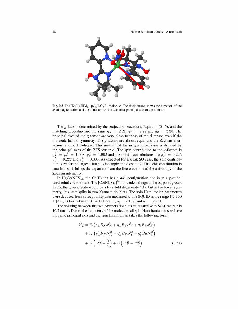
Fig. 0.3 The [Ni(II)(HIM2−py)2(NO3)]+ molecule. The thick arrows shows the direction of theaxial magnetization and the thiner arrows the two other principal axes of the d tensor.

The g-factors determined by the projection procedure, Equation (0.45), and thematching procedure are the same gX = 2.21, gY = 2.22 and gZ = 2.30. Theprincipal axes of the g tensor are very close to those of the d tensor even if themolecule has no symmetry. The g-factors are almost equal and the Zeeman inter-action is almost isotropic. This means that the magnetic behavior is dictated bythe principal axes of the ZFS tensor d. The spin contribution to the g-factors isgSX = gSY = 1.998, gSZ = 1.992 and the orbital contributions are gLX = 0.225gLY = 0.222 and gLZ = 0.306. As expected for a weak SO case, the spin contribu-tion is by far the largest. But it is isotropic and close to 2. The orbit contribution issmaller, but it brings the departure from the free electron and the anisotropy of theZeeman interaction.

In HgCo(NCS)4, the Co(II) ion has a 3d7 configuration and is in a pseudo-tetrahedral environment. The [Co(NCS)4]2– molecule belongs to the S4 point group.In Td, the ground state would be a four-fold degenerate 4A2, but in the lower sym-metry, this state splits in two Kramers doublets. The spin Hamiltonian parameterswere deduced from susceptibility data measured with a SQUID in the range 1.7-300K [48]; D lies between 10 and 11 cm−1, g‖ = 2.168, and g⊥ = 2.251.

The splitting between the two Kramers doublets calculated with SO-CASPT2 is16.2 cm−1. Due to the symmetry of the molecule, all spin Hamiltonian tensors havethe same principal axis and the spin Hamiltonian takes the following form

HS = βe

(g⊥BXSX + g⊥BY SY + g‖BZSZ

)+ βe

(g′⊥BXS 3

X + g′⊥BY S 3Y + g′‖BZS 3

Z

)+D

(S 2Z −

5

4

)+ E

(S 2X − S 2

Y

)(0.58)


The matrix g′ is reduced to its diagonal elements. The ZFS tensor d is calculatedby the effective Hamiltonian technique ; the Z axis lies along the C2 axis, and D =8.1 cm−1 and E = 0. The validity of the effective Hamiltonian procedure canbe assessed by the projection of the |λ, a〉 on the |λ′,M〉, more than 0.99 and theoverlap between the projected vectors, less than 10−4. The projection techniqueprovides the tensor A defined in Eq. 0.45 leading to g‖ = 2.173 and g⊥ = 2.255.The matching technique permits the determination of both linear and cubic terms: one gets g‖ = 2.178, g′‖ = −0.002, g⊥ = 2.263, g′⊥ = −0.004. The Zeemaninteraction is mostly isotropic and the cubic term is negligible. The two techniquesgive close but not similar g-factors due to the neglect of the cubic term in the firstone. These values are in very good agreement with the experimental ones. The spin(orbital) contributions are for g⊥ 1.992 (0.271), for g′⊥ -0.0002 (-0.004), for g‖1.989 (0.189) and for g′‖ -0.0002 (-0.002). The spin contribution is again the largest,isotropic and close to 2. The orbital one is more anisotropic and provides the onlycontribution to the cubic term. As it was the case for the Ni(II) complex, in theweak SO limit, the anisotropy of the magnetic property is determined by the ZFSinteraction.

Another description is to consider the two Kramers doublets independently, eachbeing described by a S = 1/2. One gets for the first Kramers doublet g1‖ = 2.18and g1⊥ = 4.50 and for the second one g2‖ = 6.52 and g2⊥ = 0.1. This descriptiondoes not give information on the second order Zeeman interaction between the twoKramers doublets. But in the case of a large ZFS, the transition between the twoKramers doublets can not be induced even using HFHF EPR and one only deter-mines the magnetic properties of the ground Kramers doublet. In this scheme, themagnetic anisotropy is described by the Zeeman interaction.

Another example for S = 3/2 is the NpCl2–6 cluster diluted in Cs2ZrCl6. The

Np4+ ion has a 5f3 configuration and is in an octahedral environment. The groundstate is a quartet F3/2u (using Mulliken’s notation, or Γ8 in Bethe’s notation) [49].In the principal axis system, the spin Hamiltonian takes the form

HS = βegS ·B + βeg′(BXS 3

X +BY S 3Y +BZS 3

Z

)(0.59)

Due to the cubic symmetry, HZ(1) is isotropic, HZ(3) is invariant by ’changing ’ theaxis by permutation X ←→ Y ←→ Z but is not isotropic. There are two de-grees of freedom, the two scalar g and g′ which were deduced from EPR measure-ments as g = −0.516 and g′ = 0.882. These two numbers define the magnetizationof the two pairs of Kramers doublets, 〈±3/2|µu| ± 3/2〉 = ∓( 3

2g + 278 g′) and

〈±1/2|µu| ± 1/2〉 = ∓( 12g + 1

8g′). The matching technique permits to find the

rotation R in the model space which assign the |λ, a〉 to the |S ,M 〉. One can findtwo possible assignments as was already pointed out by Bleaney, corresponding tothe permutation

{Ψ3/2 ↔ Ψ−1/2;Ψ−3/2 ↔ Ψ1/2

}. One of the solutions transforms

under rotations as a spin S = 3/2 while the other one does not. The solution givenabove fitting the EPR spectrum does not. From calculations one gets g = −0.406and g′ = 0.785. The spin and orbital contributions are 0.027 and -0.460 for g and-0.250 and 1.285 for g′. The accordance with the experimental values is reasonable.


The spin and orbital contributions are opposite, the orbital one being the largest asin the free ion. The cubic term is by far non negligible, it is larger than the linearone, and opposite in sign. Due to the high symmetry of the complex, there is noZFS. However, the cubic term plays an essential role for the Zeeman interaction.

When the complex is distorted, one gets two Kramers doublets with differentenergies. The two g-tensors are not collinear. Two pseudo-spins models can be used:Either one considers two distinct S = 1/2 each with its own g-tensor, and thetwo g-tensors are not collinear. The two spin spaces are coupled through 2nd orderZeeman interaction. It is usually the way one describes the low-energy spectra oflanthanide ions. Another way is to describe the model space as an S = 3/2 case.The g and g′ tensor are not collinear in general, and even if this space is morecomplete that the previous description, the parameters are less intuitive.

In the [FeLCl] complex with L=β-diketiminate, the Fe(II) is in 3d6 high-spinconfiguration with a S = 2 ground state. EPR measurements in the X band givesa quasidegenerate MS = ±2 ground doublet with an axial g = 10.9 and a smallsplitting of ∆ = 0.35 cm−1 . The next component of the spin quintet are estimatedto be higher than 150 cm−1 [50]. In a pure spin quintet, the MS = ±2 compo-nents have a g-factor of 6. The experimental value shows that there is a large orbitalcontribution due a partially quenching of the orbital moment and a low lying state.The CASPT2 calculation shows that without SO coupling the first excited state isanother spin quintet lying 516 cm−1 above the ground state. With the SO coupling,the spin quintet becomes a ground doublet split by 0.34 cm−1 and the other com-ponents are 118, 132 and 180 cm−1 above. The g-factors of the ground doubletmodelled with a S = 1/2 are given in Table 0.2. The magnetization is along theFe-Cl bond with g = 10.9 in perfect accordance with the experimental value. Thespin contribution of 7.99 is the expected value for a spin quintet and one noticesa large orbital contribution due to the low lying quintet state. The five componentsissued from the spin quintet may be modelled with a S = 2 pseudo-spin. In thecase where all the matrices are collinear, the spin Hamiltonian is the following

HS = βe

(gXBXSX + gYBY SY + gZBZSZ

)+ βe

(g′XBXS 3

X + g′YBY S 3Y + g′ZBZS 3

Z

)+D

(S 2Z − 2

)+ E(S 2

X − S 2Y ) +D′

(S 4Z −

34

5

)+ E′

(S 4X − S 4

Y

)(0.60)

The matrices g′ and d′ are reduced to their diagonal elements. All the spin parame-ters have been determined. Z is along the Fe−Cl axis. The g-factors and their spinand orbital contributions are summarized in Table 0.2. For the ZFS tensors, one findsD= -58.0 cm−1, E = 2.0 cm−1, D′ = 3.3 cm−1 and E′ = 0.1 cm−1. The tensor ofsecond order is largely dominant. While the rhombic term E models the splittingbetween the two MS = ±2 components, the parameter D′ of the term of fourthorder is necessary to model the whole spectrum of energy of the five pseudo-spin


Table 0.2 g-factors of FeLCl calculated with two model spaces S = 1/2 and S = 2 . gS and gL

are the spin and orbital contributions.

S = 1/2 S = 3/2g g g′

x y z x y z x y zcalc g 0.0 0.0 10.903 2.104 1.983 3.108 -0.0154 -0.013 -0.094

gS 0.0 0.0 7.994 2.000 1.965 2.000 -0.016 -0.012 0.000gL 0.0 0.0 2.909 0.104 0.018 1.108 0.002 -0.001 -0.094

exp 0.0 0.0 10.9

Table 0.3 Isotropic 199Hg HFC constants, in units of MHz, calculated with different relativisticmethods. a

HgF HgAgNR PN 9 173 2 068ZORA PN 21 958 3 404ZORA FN 19 171 3 0944-component PN 18 927 3 6904-component FN 16 895 3 285Expt. 22 163 2720

a PN = point nucleus, FN = finite nucleus (spherical Gaussian model), ZORA =zeroth-order regular approximation 2-component method. For citations of the

original data see Table 3 of Reference 51.

components. It should be noticed that, due to the large coupling with the excitedspin quintet, the projection of the five wave function in the target space is reducedto 0.89 and 0.95. For the Zeeman interaction, as in Co(NCS)4, the linear term islargely dominant and the cubic one is negligible. The spin contribution is isotropicand close to 2 while the orbital contribution is very important in the Z direction,larger than 1, and negligible in the two other ones.

Electronic EPR parameters can be calculated in many different cases. In transi-tion metal complexes, the pseudo-spin is usually the spin of the ground state. In thecase of a large ZFS, the model space can be reduced to the lower components andeffective values of g-factors are measured and calculated. When the pseudo-spin isequal to the spin, the spin contribution to the g-factor is isotropic and close to 2. Theanisotropy of g arises from orbital contributions. For large values of the pseudo-spin, the higher order terms, in S 3 for the Zeeman interaction and in S 4 the ZFSinteraction are much smaller than the S and S 2 terms. Except in the case of a lowlying excited state, the anisotropy of the magnetic properties arises from the ZFStensor, the g-factors being almost isotropic.

In the case of complexes with heavy elements, the pseudo-spin is rarely largerthan 2. Usually, the spin and orbital components are in opposite directions for lessthan filled open shells and in the same direction otherwise, as a reminiscence of thefree ion. But in the case of the quenching of some orbitals due to the interactionwith the ligands, this rule can be skewed for actinides.


-2000

-1200

-400

0

0.25 0.5 0.75 1 1.25

Ais

o / M

Hz

SO scaling factor λ

NpF6

PBE

HF

Fig. 0.4 237Np HFC constant of NpF6 versus scaling of SO Hamiltonian integrals in the groundstate calculation (λ = 0 means SR, λ = 1 means full SO). HF and DFT calculations (PBE func-tional) of Ref. 30 utilizing Eq. (0.22).

Regarding HFC, there are few examples highlighting the role of relativistic ef-fects and finite nuclear volume effects better than 199Hg. Table 0.3 lists a collectionof calculated (DFT, with a hybrid functional for NR and ZORA and a non-hybridfunctional for the 4-component calculations) and experimental data for the radicalsHgH and HgF. The increase of the Hg HFC from NR to relativistic calculations,in particular for HgH, is rather spectacular. The effect is mainly due to SR effectsfrom the relativistic increase of the spin density at the Hg nucleus. The effects froma finite nuclear volume are also very large, roughly on the order of 10% relative tothe total, and decrease the HFC. SO effects on mercury HFC constants tend to berelatively minor because it is dominated by contributions from the Hg 6s orbital.

The situation is different for the 5f1 complex 237Np and 19F HFC constants ofNpF6. Experimentally, the isotropic HFC constants were found to be −1995 MHzfor 237Np and−73 MHz for 19F. For Np, the HFC tensor is isotropic due to the octa-hedral symmetry of the complex. For 19F, there are two unique tensor components,a‖ in the direction of the Np–F axes and a degenerate pair of a⊥ perpendicular to theNp–F axes, with a‖ = −132, a⊥ = −42 MHz experimentally. The unpaired elec-tron is described at the SR level by a non-bonding Np 5f orbital of δ symmetry withrespect to the Np–F axes. Without SO coupling, the isotropic Np HFC is calculatedto be much too small in magnitude, by a factor of 3 to 5 depending on the compu-tational method. Spin polarization is responsible for the residual Np HFC and mostof the fluorine HFC at the SR level. Under the SO interaction, there is a very dom-inant contribution to the Np HFC from the PSO mechanism. This mechanism canbe interpreted as follows: Via SO coupling, the unpaired spin at Np creates a para-magnetic orbital current density in the 5f shell which then interacts magneticallywith the nuclear spin. The NMR shielding tensors for diamagnetic molecules afforda similar mechanism, except that a paramagnetic orbital current density is inducedby the external magnetic field rather than via an unpaired spin and SO coupling.

Figure 0.4 shows the 237Np HFC constant for NpF6 calculated with HF theory andDFT using Equation (0.22). The horizontal axis indicates a parameter λ used to scalethe SO Hamiltonian integrals in the ground state calculations, meaning that λ = 0


gives the SR limit. The fact that the data exhibit significant curvatures show thatSO effects beyond first order are important and reduce the HFC magnitude. Indeed,calculations where SO coupling is treated with a linear-response method (to producethe PSO mechanism) over-estimate the Np HFC by 15% or more, depending on thefunctional used for the calculations. Further details and citations of prior studieswhere such SO scaling has been used can be found in Reference 30.

For 19F, CASSCF calculations recently indicated [52] that without SO couplingthe HFC tensor anisotropy is not correctly predicted. With SO coupling, the cal-culations predict a‖ to be twice as large in magnitude as a⊥, with the latter closeto experiment. The magnitude of the calculated a‖ appears to be underestimated.However, the measurements were performed on a solid, with NpF6 diluted in a UF6host crystal, while the calculations were for an isolated molecule. It is presentlyunknown precisely how solid state packing affects the fluorine HFC tensors.

The CAS calculations of g-tensors and ZFS discussed above were performedwith the MOLCAS suite of programs. For the benefit of the reader, details of thecomputations are given here. NpO2+

2 , [NpO2(NO3)3]−, [NpO2Cl4]2−, PuO2+2 and

[PuO2(NO3)3]–: Results are given with ano.rcc basis sets of TZP quality at the SO-CASPT2 level with CAS(7,10) comprising the 7 5f orbitals and the two bonding σand π orbitals. The environment is described by ECP and point charges. The stateinteraction for the calculation of the SO coupling is performed with 6 spin doublets.[Ni(II)(HIM2−py)2(NO3)]+: Results are given with ano.rcc basis sets of TZP qual-ity on the Ni and DZP on the ligands at the SO-CASPT2 level with CAS(8,10)comprising the 8 3d electrons within a double shell of d orbitals. The state interac-tion for the calculation of SO coupling is performed with 10 triplets and 15 singlets.Similar calculations are published in reference [53]. HgCo(NCS)4: Calculationsare performed with ano.rcc basis sets of TZP quality for the [Co(NCS)4]2– com-plex. The complex is embedded in point charges describing the rest of the crystal.Hg2+ ions are described by ECPs and other ions by point charges within a radiusof 10 A. The cluster is described at the SO-CASPT2 level with 10 spin quartetsand 40 spin doublets using a CAS(7,5) (7 electrons in the 5 3d orbitals). NpCl2–

6 :Calculations are performed with ano.rcc basis sets of TZP quality for the [NpCl6]2–

complex. The complex is embedded in point charges and model potentials describ-ing the rest of the crystal. Hg2+ ions are described by ECPs and other ions by pointcharges. The cluster is described at the SO-CASPT2 level with 35 quartets and 84doublets using a CAS(3,7) (3 electrons in the 7 5f orbitals). [LFeCl]: Results aregiven with ano.rcc basis sets of TZP quality on the Fe and DZP on the ligands atthe SO-CASPT2 level with CAS(6,5) comprising the 6 3d electrons within the 5 3dorbitals. The state interaction for the calculation of SO coupling is performed with5 quintets, 15 triplets and 10 singlets.


0.6 Summary

There is a large variety of techniques available for ab-initio calculations of EPR pa-rameters. Nonetheless, it can be a complicated task to extract EPR spin Hamiltonianparameters from ab-initio calculations if SO coupling is strong, if the degeneracy ofthe state of interest is higher than two-fold, or for non-Kramers doublets. In the limitof weak SO coupling, the effective Hamiltonian technique is well established. Forstrong SO coupling, the wavefunctions should include SO coupling variationally orvia state interaction. KS methods can be an effective alternative to wavefunctionbased methods.

Acknowledgements J.A. acknowledges support of his research on EPR and NMR parametersof open-shell heavy metal complexes by the U.S. Department of Energy, Office of Basic EnergySciences, Heavy Element Chemistry program, under grant DE-FG02-09ER16066.

Key words: Electron paramagnetism, electron paramagnetic resonance, spinHamiltonian, spin orbit coupling, hyperfine coupling, electron g-factor, Zeemaninteraction, electron spin, nuclear spin, finite nucleus effects

References

1. N.M. Atherton, Principles of Electron Spin Resonance. Ellis Horwood series in physicalchemistry (Prentice Hall, New York, 1993)

2. P.H. Rieger, Electron spin resonance. Analysis and interpretation (The Royal Society ofChemistry, Cambridge, UK, 2007)

3. J.E. Harriman, Theoretical foundations of electron spin resonance (Academic Press, NewYork, 1978)

4. A. Abragam, B. Bleaney, Electron paramagnetic resonance of transition ions (ClarendonPress, Oxford, 1970)

5. P.J. Mohr, B.N. Taylor, D.B. Newell, Rev. Mod. Phys. 84, 1527 (2012)6. J.E. Butler, C.A. Hutchison, Jr., J. Chem. Phys. 74(6), 3102 (1981)7. J.S. Griffith, Mol. Phys. 12, 359 (1967)8. F. Neese, E.I. Solomon, Inorg. Chem. 37, 6568 (1998)9. H. Bolvin, ChemPhysChem 7, 1575 (2006)

10. L.F. Chibotaru, L. Ungur, J. Chem. Phys. 137, 064112 (2012)11. L.F. Chibotaru, Adv. Chem. Phys. 153, 397 (2013)12. B.O. Roos, P.R. Taylor, P.E.M. Siegbahn, Chem. Phys. 48, 157 (1980)13. K. Andersson, P.A. Malmqvist, B.O. Roos, A.J. Sadlej, K. Wolinski, J. Phys. Chem. 94, 5483

(1990)14. C. Angeli, R. Cimiraglia, J.P. Malrieu, J. Chem. Phys. 117, 9138 (2002)15. T.N. Lan, Y. Kurashige, T. Yanai, J. Chem. Theory Comput. 10, 1953 (2014)16. B. Fernandez, P. Jørgensen, J. Byberg, J. Olsen, T. Helgaker, H.J.A. Jensen, J. Chem. Phys.

97(5), 3412 (1992)17. P.A. Malmqvist, B.O. Roos, Chem. Phys. Lett. 155, 189 (1989)18. M.S. Vad, P.M. N., A. Nørager, H.J.A. Jensen, J. Chem. Phys. 138, 214106 (2013)19. W. Kutzelnigg, Z. Phys. D 15, 27 (1990)20. J.P. Perdew, A. Ruzsinszky, L.A. Constantin, J. Sun, G.I. Csonka, J. Chem. Theory Comput.

5(4), 902 (2009)


21. L.A. Eriksson, in Encyclopedia of Computational Chemistry, ed. by P. von Rague Schleyer(Wiley, Chichester, UK, 1998), pp. 952–958

22. S. Patchkovskii, G. Schreckenbach, in Calculation of NMR and EPR Parameters. Theory andApplications, ed. by M. Kaupp, M. Buhl, V.G. Malkin (Wiley-VCH, Weinheim, 2004), pp.505–532

23. M. Kaupp, F.H. Kohler, Coord. Chem. Rev. 253(19-20), 2376 (2009)24. F. Neese, Coord. Chem. Rev. 253(5-6), 526 (2009)25. T. Helgaker, S. Coriani, P. Jørgensen, K. Kristensen, J. Olsen, K. Ruud, Chem. Rev. 112, 543

(2012)26. J. Autschbach, T. Ziegler, Coord. Chem. Rev. 238/239, 83 (2003)27. J. Autschbach, in Relativistic Methods for Chemists, Challenges and Advances in Com-

putational Chemistry and Physics, vol. 10, ed. by M. Barysz, Y. Ishikawa (Springer,Dordrecht, 2010), chap. 12, pp. 521–598. URL http://dx.doi.org/10.1007/978-1-4020-9975-5_12

28. E. van Lenthe, P.E.S. Wormer, A. van der Avoird, J. Chem. Phys. 107, 2488 (1997)29. E. Malkin, M. Repisky, S. Komorovsky, P. Mach, O.L. Malkina, V.G. Malkin, J. Chem. Phys.

134(4), 044111 (2011)30. P. Verma, J. Autschbach, J. Chem. Theory Comput. 9, 1932 (2013)31. S. Schmitt, P. Jost, C. van Wullen, J. Chem. Phys. 134(19), 194113 (2011)32. C. van Wullen, J. Chem. Phys. 130(19), 194109 (2009)33. J. Autschbach, J. Chem. Phys. 136, 150902 (2012)34. L. Visscher, K. Dyall, At. Data Nucl. Data Tables 67(2), 207 (1997)35. W. Van den Heuvel, A. Soncini, Phys. Rev. Lett. 109, 073001 (2012)36. C. Rodowicz, Nukleonika 58, 341 (2013)37. R. Maurice, R. Bastardis, C. de Graaf, N. Suaud, T. Mallah, N. Guihery, J. Chem. Theory

Comput. 11, 2977 (2009)38. M.H.L. Pryce, Phys. Rev. Lett. 3, 375 (1959)39. J.D. Axe, H.J. Stapleton, C.D. Jefries, Phys. Rev. 121, 1630 (1961)40. P. Rigny, P. Plurien, J. Phys. Chem. Solids 28, 2589 (1967)41. J.C. Eisenstein, M.H.L. Pryce, J. Res. Natl. Bur. Stand. Sect. A 69A, 217 (1965)42. L.F. Chibotaru, L. Ungur, Phys. Rev. Lett. 109, 246403 (2012)43. L. Chibotaru, A. Ceulemans, H. Bolvin, Phys. Rev. Lett. 101, 033003 (2008)44. F.P. Notter, H. Bolvin, J. Chem. Phys. 130, 184310 (2009)45. F. Gendron, D. Paez Hernandez, F.P. Notter, B. Pritchard, H. Bolvin, J. Autschbach, Chem.

Eur. J. 20, 7994 (2014)46. F. Gendron, B. Pritchard, H. Bolvin, J. Autschbach, Inorg. Chem. 53, 8577 (2014)47. G. Rogez, J.N. Rebilly, A.L. Barra, L. Sorace, G. Blondin, N. Kirchner, M. Duran, J. van

Slageren, S. Parsons, L. Ricard, A. Marvilliers, T. Mallah, Angew. Chem. 44, 1876 (2005)48. D. Nelson, L.W. ter Haar, Inorg. Chem. 32, 182 (1993)49. D. Paez Hernandez, H. Bolvin, J. Electron. Spectrosc. Relat. Phenom. 194, 74 (2014)50. H. Andres, E.L. Bominaar, J.M. Smith, N.A. Eckert, P.L. Holland, E. Mnck, J. Am. Chem.

Soc. 124, 3012 (2002)51. J. Autschbach, J. Phil. Trans. A 372, 20120489 (2014)52. K. Sharkas, J. Autschbach, J. Chem. Theory Comput. p. in press. http://dx.doi.org/

10.1021/ct500988h53. L. Chibotaru, L. Ungur, J. Chem. Phys. 137, 064112 (2012)

Relativistic Methods for Calculating Electron Paramagnetic ...

Documents

Transcript of Relativistic Methods for Calculating Electron Paramagnetic ...