Calculating two-point resistances in distance-regular resistor ...

arX

iv:c

ond-

mat

/061

1683

v1 [

cond

-mat

.sta

t-m

ech]

27

Nov

200

6

Calculating two-point resistances in

distance-regular resistor networks

M. A. Jafarizadeha,b,c ∗, R. Sufiania,c, S. Jafarizadehd †

aDepartment of Theoretical Physics and Astrophysics, Tabriz University, Tabriz 51664, Iran.

bInstitute for Studies in Theoretical Physics and Mathematics, Tehran 19395-1795, Iran.

cResearch Institute for Fundamental Sciences, Tabriz 51664, Iran.

dDepartment of Electrical and computer engineering, Tabriz University, Tabriz 51664, Iran.

June 29, 2018

∗E-mail:[email protected]

†E-mail:[email protected]

1

http://arxiv.org/abs/cond-mat/0611683v1

Two-point resistance 2

Abstract

An algorithm for the calculation of the resistance between two arbitrary nodes in an

arbitrary distance-regular resistor network is provided, where the calculation is based on

stratification introduced in [1] and Stieltjes transform of the spectral distribution (Stielt-

jes function) associated with the network. It is shown that the resistances between a

node α and all nodes β belonging to the same stratum with respect to the α (Rαβ(i) , β

belonging to the i-th stratum with respect to the α) are the same. Also, the analytical

formulas for two-point resistances Rαβ(i) , i = 1, 2, 3 are given in terms of the the size of the

network and corresponding intersection numbers. In particular, the two-point resistances

in a strongly regular network are given in terms of the its parameters (v, κ, λ, µ). More-

over, the lower and upper bounds for two-point resistances in strongly regular networks

are discussed.

Keywords:two-point resistance, association scheme, distance-regular net-

works, Stieltjes function

PACs Index: 01.55.+b, 02.10.Yn


1 Introduction

A classic problem in electric circuit theory studied by numerous authors over many years is

the computation of the resistance between two nodes in a resistor network (see, e.g., [2]).

Besides being a central problem in electric circuit theory, the computation of resistances is

also relevant to a wide range of problems ranging from random walks (see [3]), the theory of

harmonic functions [4], to lattice Greens functions [5, 6, 7, 8, 9]. The connection with these

problems originates from the fact that electrical potentials on a grid are governed by the same

difference equations as those occurring in the other problems. For this reason, the resistance

problem is often studied from the point of view of solving the difference equations, which is

most conveniently carried out for infinite networks. In the case of Greens function approach,

for example, past efforts [2], [23] have been focused mainly on infinite lattices. Little attention

has been paid to finite networks, even though the latter are those occurring in real life. In this

paper, we take up this problem and present a general formulation for computing two-point

resistances in finite networks. Particularly, we show that known results for infinite networks

are recovered by taking the infinite-size limit.

The study of electric networks was formulated by Kirchhoff [11] more than 150 years ago

as an instance of a linear analysis. Our starting point is along the same line by considering the

Laplacian matrix associated with a network. The Laplacian is a matrix whose off-diagonal en-

tries are the conductances connecting pairs of nodes. Just as in graph theory where everything

about a graph is described by its adjacency matrix (whose elements is 1 if two vertices are

connected and 0 otherwise), everything about an electric network is described by its Laplacian.

The author of [12], has been derived an expression for the two-point resistance between two

arbitrary nodes α and β of a regular network in terms of the matrix entries L−1αα, L

−1ββ and

L−1αβ , where L

−1 is the pseudo inverse of the Laplacian matrix. Here in this work, based on

stratification introduced in [1] and spectral analysis method, we introduce an procedure for


calculating two-point resistances in distance-regular resistor networks in terms of the Stieltjes

function Gµ(x) associated with the adjacency matrix of the network and its derivatives. Al-

though, we discuss the case of distance-regular networks, but also the method can be used for

any arbitrary regular network. It should be noticed that, in this way, the two-point resistances

are calculated straightforwardly without any need to know the spectrum of the network. Also,

it is shown that the resistances between a node α and all nodes β belonging to the same stra-

tum with respect to the α (Rαβ(i) , β belonging to the i-th stratum with respect to the α) are

the same. We give the analytical formulas for two-point resistances Rαβ(i) , i = 1, 2, 3 in terms

of the network’s characteristics such as the size of the network and its intersection array. In

particular, the two-point resistances in a strongly regular network are given in terms of the

network’s parameters (v, κ, λ, µ). Moreover, we discuss the lower and upper bounds for two-

point resistances in strongly regular networks. From the fact that, the two-point resistances on

a network depend on the corresponding Stieltjes function Gµ(x) and that Gµ(x) is written as a

continued fraction, the two-point resistances on an infinite-size network can be approximated

with those of the corresponding finite-size networks.

The organization of the paper is as follows. In section 2, we give some preliminaries such

as association schemes, distance-regular networks, stratification of these networks and Stieltjes

function associated with the network. In section 3, two-point resistances in distance-regular

networks are given in terms of the Stieltjes function and its derivatives. Also, the resistances

Rαβ(i) , for i = 1, 2, 3 are given in terms of the network’s intersection array. In particular, two-

point resistances in a strongly regular network are given in terms of the network’s parameters,

also lower and upper bounds for the two-point resistances in these networks are discussed. Sec-

tion 4 is devoted to calculating two-point resistances Rαβ(i) for i = 1, 2, 3 in some important

examples of distance-regular networks, such as complete network, strongly regular networks

(distance-regular networks with diameter 2), e.g. Petersen and normal subgroup scheme net-

works [1], d-cube (d dimensional hypercube) and Johnson networks. The paper is ended with a


brief conclusion and an appendix containing a table for two-point resistances Rαβ(i) , i = 1, 2, 3

of some important distance-regular resistor networks with size less than 70.

2 Preliminaries

In this section we give some preliminaries such as definitions related to association schemes,

corresponding stratification, distance-regular networks and Stieltjes function associated with

the network.

2.1 Association schemes

First we recall the definition of association schemes. The reader is referred to Ref.[13], for

further information on association schemes.

Definition 2.1 (Symmetric association schemes). Let V be a set of vertices, and let Ri(i =

0, 1, ..., d) be nonempty relations on V (i.e., subset of V ×V ). Let the following conditions (1),

(2), (3) and (4) be satisfied. Then, the relations {Ri}0≤i≤d on V × V satisfying the following

conditions

(1) {Ri}0≤i≤d is a partition of V × V

(2) R0 = {(α, α) : α ∈ V }

(3) Ri = Rti for 0 ≤ i ≤ d, where Rt

i = {(β, α) : (α, β) ∈ Ri}

(4) For (α, β) ∈ Rk, the number pki,j =| {γ ∈ X : (α, β) ∈ Ri and (γ, β) ∈ Rj} | does not

depend on (α, β) but only on i, j and k,

define a symmetric association scheme of class d on V which is denoted by Y = (V, {Ri}0≤i≤d).

Furthermore, if we have pkij = pkji for all i, j, k = 0, 2, ..., d, then Y is called commutative.

The intersection number pkij can be interpreted as the number of vertices which have relation

i and j with vertices α and β, respectively provided that (α, β) ∈ Rk, and it is the same for

all element of relation Rk. For all integers i (0 ≤ i ≤ d), set ki = p0ii and note that ki 6= 0,


since Ri is non-empty. We refer to ki as the i-th valency of Y .

Let Y = (X, {Ri}0≤i≤d) be a commutative symmetric association scheme of class d, then

the matrices A0, A1, ..., Ad defined by

(Ai)α,β =

1 if (α, β) ∈ Ri

0 otherwise, (2-1)

are adjacency matrices of Y such that

AiAj =d

∑

k=0

pkijAk. (2-2)

From (2-2), it is seen that the adjacency matrices A0, A1, ..., Ad form a basis for a commutative

algebra A known as the Bose-Mesner algebra of Y .

Definition 2.2 (P -polynomial property) Y = (X, {Ri}0≤i≤d) is said to be P -polynomial (with

respect to the ordering R0, ..., Rd of the associate classes) whenever for all integers h, i, j (0 ≤

h, i, j ≤ d),

phij = 0 if one of h, i, j is greater than the sum of the other two,

phij 6= 0 if one of h, i, j equals the sum of the other two. (2-3)

It is shown in [14] that in the case of P-polynomial schemes, Ai = Pi(A) (0 ≤ i ≤ d), where

Pi is a polynomial with real coefficients and degree exactly i. In particular, A multiplicatively

generates the Bose-Mesner algebra.

Finally the underlying graph of an association scheme Γ = (V,R1) is an undirected con-

nected graph, where the set V and R1 consist of its vertices and edges, respectively. Obviously

replacing R1 with one of other relation such as Ri, for i 6= 0, 1 will also give us an underlying

graph Γ = (V,Ri) (not necessarily a connected graph ) with the same set of vertices but a new

set of edges Ri.


2.2 Stratifications

For a given vertex α ∈ V , let Ri(α) := {β ∈ V : (α, β) ∈ Ri} denote the set of all vertices

having the relation Ri with α. Then, the vertex set V can be written as disjoint union of Ri(α)

for i = 0, 1, 2, ..., d, i.e.,

V =d⋃

i=0

Ri(α). (2-4)

We fix a point o ∈ V as an origin of a distance regular graph (the underlying graph of an

association scheme), called reference vertex. Then, the relation (2-4) stratifies the underlying

graph into a disjoint union of associate classes Ri(o). With each associate class Ri(o) we

associate a unit vector in l2(V ) defined by

|φi〉 =1√κi

∑

α∈Ri(o)

|α〉, (2-5)

where, |α〉 denotes the eigenket of α-th vertex at the associate class Ri(o) and κi = |Ri(o)| is

called the i-th valency of the graph (i.e., κi = p0i,i). The closed subspace of l2(V ) spanned by

{|φi〉} is denoted by Λ(G). Since {|φi〉} becomes a complete orthonormal basis of Λ(G), we

often write

Λ(G) =∑

i

⊕C|φi〉. (2-6)

Let Ai be the adjacency matrix of a graph Γ = (V,R) for reference state |φ0〉 (|φ0〉 = |o〉, with

o ∈ V as reference vertex), we have

Ai|φ0〉 =∑

β∈Ri(o)

|β〉. (2-7)

Then by using unit vectors |φi〉 (2-5) and (2-7), we have

Ai|φ0〉 =√κi|φi〉. (2-8)

2.3 Distance-regular graphs

Here in this section we consider some set of important graphs called distance regular graphs,

where the relations are based on distance function defined as follows: A finite sequence


α0, α1, ..., αn ∈ V is called a walk of length n (or of n steps) if αk−1 ∼ αk for all k = 1, 2, ..., n.

For α 6= β let ∂(α, β) be the length of the shortest walk connecting α and β, therefore ∂(α, β)

gives the distance between vertices α and β hence it is called the distance function and we

have ∂(α, α) = 0 for all α ∈ V and ∂(α, β) = 1 if and only if α ∼ β. Therefore, the distance

regular graphs become metric spaces with the distance function ∂.

An undirected connected graph Γ = (V,R1) is called distance regular graph if it is the

underlying graph of a P -polynomial association scheme with relations defined as: (α, β) ∈ Ri

if and only if ∂(α, β) = i, for i = 0, 1, ..., d, where d :=max{∂(α, β) : α, β ∈ V } is called the

diameter of the graph. Usually in distance regular graphs, the relations Ri are denoted by Γi.

Now, in any connected graph, for every β ∈ Ri(α) we have

R1(β) ⊆ Ri−1(α) ∪ Ri(α) ∪ Ri+1(α). (2-9)

Hence in a distance regular graph, pij1 = 0 (for i 6= 0, j is not {i−1, i, i+1}). The intersection

numbers of the graph are defined as

ai = pii1, bi = pii+1,1, ci = pii−1,1 . (2-10)

The intersection numbers (2-10) and the valencies κi satisfy the following obvious conditions

ai + bi + ci = κ, κi−1bi−1 = κici, i = 1, ..., d,

κ0 = c1 = 1, b0 = κ1 = κ, (c0 = bd = 0). (2-11)

Thus all parameters of the graph can be obtained from the intersection array {b0, ..., bd−1; c1, ..., cd}.

It should be noticed that, for distance-regular graphs, the unit vectors |φi〉 for i = 0, 1, ..., d

defined as in (2-5), satisfy the following three-term recursion relations

A|φi〉 = βi+1|φi+1〉+ αi|φi〉+ βi|φi−1〉, (2-12)

where, the coefficients αi and βi are defined as

αk = κ− bk − ck, ωk ≡ β2k = bk−1ck, k = 1, ..., d, (2-13)


i.e., in the basis of unit vectors {|φi〉, i = 0, 1, ..., d}, the adjacency matrix A is projected to

the following symmetric tridiagonal form:

A =

α0 β1 0 ... ... 0

β1 α1 β2 0 ... 0

0 β2 α3 β3. . .

...

.... . .

. . .. . .

. . . 0

0 . . . 0 βd−1 αd−1 βd

0 ... 0 0 βd αd

. (2-14)

In Ref. [20], it has be shown that, the coefficients αi and βi can be also obtained easily by

using the Lanczos iteration algorithm. Hereafter, we will refer to the parameters αi and ωi in

(2-13) as QD (Quantum decomposition) parameters.

One should notice that, in distance regular graphs stratification is reference state indepen-

dent, namely we can choose every vertex as a reference state, while the stratification of more

general graphs may be reference dependent.

2.4 Stieltjes function associated with the network

It is well known that, for any pair (A, |φ0〉) of a matrix A and a vector |φ0〉, it can be assigned

a measure µ as follows

µ(x) = 〈φ0|E(x)|φ0〉, (2-15)

where E(x) =∑

i |ui〉〈ui| is the operator of projection onto the eigenspace of A corresponding

to eigenvalue x, i.e.,

A =∫

xE(x)dx. (2-16)

It is easy to see that, for any polynomial P (A) we have

P (A) =∫

P (x)E(x)dx, (2-17)


where for discrete spectrum the above integrals are replaced by summation. Therefore, using

the relations (2-15) and (2-17), the expectation value of powers of adjacency matrix A over

starting site |φ0〉 can be written as

〈φ0|Am|φ0〉 =∫

Rxmµ(dx), m = 0, 1, 2, .... (2-18)

The existence of a spectral distribution satisfying (2-18) is a consequence of Hamburgers the-

orem, see e.g., Shohat and Tamarkin [[15], Theorem 1.2].

Obviously relation (2-18) implies an isomorphism from the Hilbert space of the stratification

onto the closed linear span of the orthogonal polynomials with respect to the measure µ. It is

well known that [20] for distance-regular graphs we have

|φi〉 = Pi(A)|φ0〉, (2-19)

where Pi is a polynomial with real coefficients and degree i. Now, substituting (2-19) in (2-12),

we get three term recursion relations between polynomials Pj(A), which leads to the following

three term recursion between polynomials Pj(x)

xPk(x) = βk+1Pk+1(x) + αkPk(x) + βkPk−1(x) (2-20)

for k = 0, ..., d− 1, with P0(x) = 1.

Multiplying by β1...βk we obtain

β1...βkxPk(x) = β1...βk+1Pk+1(x) + αkβ1...βkPk(x) + β2k .β1...βk−1Pk−1(x). (2-21)

By rescaling Pk as Qk = β1...βkPk, the spectral distribution µ under question is characterized

by the property of orthonormal polynomials {Qk} defined recurrently by

Q0(x) = 1, Q1(x) = x,

xQk(x) = Qk+1(x) + αkQk(x) + β2kQk−1(x), k ≥ 1. (2-22)


If such a spectral distribution is unique, the spectral distribution µ is determined by the

identity

Gµ(x) =∫

R

µ(dy)

x− y=

1

z − α0 − β21

z−α1−β22

z−α2−β23

z−α3−···

=Q

(1)d−1(x)

Qd(x)=

d−1∑

l=0

Al

x− xl, (2-23)

where, xl are the roots of polynomial Qd(x). Gµ(z) is called the Stieltjes/Hilbert transform of

spectral distribution µ or Stieltjes function and polynomials {Q(1)k } are defined recurrently as

Q(1)0 (x) = 1, Q

(1)1 (x) = x− α1,

xQ(1)k (x) = Q

(1)k+1(x) + αk+1Q

(1)k (x) + β2

k+1Q(1)k−1(x), k ≥ 1, (2-24)

respectively. The coefficients Al appearing in (2-23) are calculated as

Al = limz→xl

(z − xl)Gµ(z). (2-25)

(for more details see Refs.[15, 16, 17, 18].)

3 Two-point resistances in regular resistor networks

A classic problem in electric circuit theory studied by numerous authors over many years, is

the computation of the resistance between two nodes in a resistor network (see, e.g., [2]). The

results obtained in this section show that, there is a close connection between the techniques

introduced in section 2 such as Hilbert space of the stratification and the Stieltjes function

and electrical concept of resistance between two arbitrary nodes of regular networks and these

techniques can be employed for calculating two-point resistances.

For a given regular graph Γ with n vertices and adjacency matrix A, let rij = rji be the

resistance of the resistor connecting vertices i and j. Hence, the conductance is cij = r−1ij = cji

so that cij = 0 if there is no resistor connecting i and j. Denote the electric potential at the

i-th vertex by Vi and the net current flowing into the network at the i-th vertex by Ii (which


is zero if the i-th vertex is not connected to the external world). Since there exist no sinks

or sources of current including the external world, we have the constraint∑n

i=1 Ii = 0. The

Kirchhoff law statesn∑

j=1,j 6=i

cij(Vi − Vj) = Ii, i = 1, 2, ..., n. (3-26)

Explicitly, Eq.(3-26) reads

L~V = ~I, (3-27)

where, ~V and ~I are n-vectors whose components are Vi and Ii, respectively and

L =∑

i

ci|i〉〈i| −∑

i,j

cij |i〉〈j| (3-28)

is the Laplacian of the graph Γ with

ci ≡n∑

j=1,j 6=i

cij , (3-29)

for each vertex α. Hereafter, we will assume that all nonzero resistances are equal to r, then

the off-diagonal elements of −L are precisely those of 1rA, i.e.,

L =1

r(κI − A), (3-30)

with κ = deg(α), for each vertex α. It should be noticed that, L has eigenvector (1, 1, ..., 1)t

with eigenvalue 0. Therefore, L is not invertible and so we define the psudo-inverse of L as

L−1 =∑

i,λi 6=0

λ−1i Ei, (3-31)

where, Ei is the operator of projection onto the eigenspace of L−1 corresponding to eigenvalue

λi. Following the result of [12] and that L−1 is a real matrix, the resistance between vertices

α and β is given by

Rαβ = 〈α|L−1|α〉 − 2〈α|L−1|β〉+ 〈β|L−1|β〉. (3-32)

In this paper, we will consider distance-regular graphs as resistor networks. Then, the diag-

onal entries of L−1 are independent of the vertex, i.e., L−1αα = L−1

ββ for all α, β ∈ V . Therefore,


from the relation (3-32), we can obtain the two-point resistance between two arbitrary nodes

α and β as follows is written as

Rαβ = 2(L−1αα − L−1

αβ). (3-33)

Now, let α and β be two arbitrary nodes of the network such that β belongs to the l-th

stratum with respect to α, i.e., β ∈ Rl(α) (we choose one of the nodes, here α, as reference

node). Then, for calculating the matrix entries L−1αα and L−1

βα in (3-32), we use the Stieltjes

function to obtain

L−1αα = r〈α| 1

κI −A|α〉 = r

∫

R−{κ}

dµ(x)

κ− x= r

d−1∑

i,i 6=0

Ai

κ− xi= r lim

y→κ(Gµ(y)−

A0

y − κ) (3-34)

and

L−1βα = r〈β| 1

κI − A|α〉 = r√

κl〈φl|

1

κI −A|α〉 = r√

κl〈α| Pl(A)

κI −A|α〉

=r√κl

∫

R−{κ}

dµ(x)

κ− xPl(x) =

r√κl

∑

i,i 6=0

AiPl(xi)

κ− xi, (3-35)

where, we have considered x0 = κ (κ is the eigenvalue corresponding to the idempotent E0).

Then, by using (3-33), the two-point resistance Rαβ(l) in the network is given by

Rαβ(l) =2r√κl(√κl lim

y→κ(Gµ(y)−

A0

y − κ)−

∑

i,i 6=0

AiPl(xi)

κ− xi). (3-36)

For evaluating the term∑

i,i 6=0AiPl(xi)κ−xi

in (3-36), we need to calculate

Im :=∑

i,i 6=0

Aixmi

κ− xi, for m = 0, 1, ..., l. (3-37)

To do so, we write the term (3-37) as

Im =∑

i,i 6=0

Aixmi

κ− xi=

∑

i,i 6=0

Ai((xi − κ)m −∑ml=1(−1)lCm

l κlxm−l

i )

κ− xi

= −∑

i,i 6=0

Ai(xi − κ)m−1 −m∑

l=1

(−1)lCml κ

l∑

i,i 6=0

Aixm−li

κ− xi, (3-38)

that is, we have

Im = −m−1∑

l=0

(−1)lCm−1l κl

∑

i,i 6=0

Aixm−l−1i −

m∑

l=1

(−1)lCml κ

lIm−l. (3-39)


Therefore, Im can be calculated recursively, if we able to calculate the term∑

i,i 6=0Aixm−l−1i

for l = 0, 1, ..., m− 1 appearing in (3-38). For example, for m = 1, we obtain

I1 =∑

i,i 6=0

Aixiκ− xi

= −∑

i,i 6=0

Ai + κI0 = −1 + A0 + κ∑

i,i 6=0

Ai

κ− xi. (3-40)

In order to evaluation of the sum∑

i,i 6=0Aixki , we rescale the roots xi as ξxi, where ξ is some

nonzero constant. Then, we will have

1

ξGµ(x/ξ) =

∑

i

Ai

x− ξxi+

A0

x− ξx0. (3-41)

Now, we take the m-th derivative of (3-41) to obtain

∂m

∂ξm(1

ξGµ(x/ξ)) = m!(

∑

i,i 6=0

Aixmi

(x− ξxi)m+1+

A0xm0

(x− ξx0)m+1), (3-42)

where, at the limit of the large x, one can obtain the following simple form

limx→∞

∂m

∂ξm(1

ξGµ(x/ξ)) = m!(

∑

i,i 6=0Aixmi + A0x

m0

xm+1) (3-43)

Therefore, we obtain

∑

i,i 6=0

Aixmi =

1

m!limx→∞

[xm+1 ∂m

∂ξm(1

ξGµ(x/ξ))]−A0x

m0 . (3-44)

3.1 Two-point resistances up to the third stratum

In this subsection we give analytical formulas for two-point resistances Rαβ(i) , i = 1, 2, 3, in

terms of intersection numbers.

It should be noticed that, for two arbitrary nodes α and β such that β ∈ R1(α), we have

P1(x) =x√κ. Therefore, by using (3-35) and (3-40) we obtain

L−1βα =

r

κ

∑

i,i 6=0

Aixiκ− xi

=−rκ

∑

i,i 6=0

Ai + r∑

i,i 6=0

Ai

κ− xi. (3-45)

Therefore, by using (3-33), we obtain the following simple result for all β ∈ R1(α)

Rαβ(1) =2r

κ

∑

i,i 6=0

Ai =2r

κ(1− A0) =

2r

κ(1− 1

v), (3-46)


where, v is the number of vertices of the graph, and in the last equality we have used the fact

that for regular graphs, we have

A0 =1

v. (3-47)

In the following, we give analytical formulas for calculating two-point resistances Rαβ(2) and

Rαβ(3) , where Rαβ(2)(Rαβ(3)) denotes the mutual resistances between α and all β ∈ R2(α) (all

β ∈ R3(α)).

By using (2-22) and that Pk = Qk√ω1...ωk

, we have P2(x) =1√ω1ω2

(x2 −α1x−ω1). Then, from

(3-35) after some simplifications we obtain for β ∈ R2(α)

L−1αβ(2) =

r√ω1ω2κ2

(−∑

i,i 6=0

Aixi + (α1 − κ)∑

i,i 6=0

Ai + κ(κ− α1 − 1)∑

i,i 6=0

Ai

κ− xi). (3-48)

By substituting α1 = κ− b1 − c1 in κ(κ− α1 − 1), we obtain

κ(κ− α1 − 1) = κ(b1 + c1 − 1) = κb1. (3-49)

Then, the coefficient of the term∑

i,i 6=0Ai

κ−xiin (3-48) is

rκb1√ω1ω2κ2

=rκb1√κb1c2κ2

= r

√

κb1c2κ2

= r. (3-50)

Therefore, (3-48) can be written as

L−1αβ(2) =

r√ω1ω2κ2

(−∑

i,i 6=0

Aixi + (α1 − κ)∑

i,i 6=0

Ai) + r∑

i,i 6=0

Ai

κ− xi, (3-51)

where, the sum∑

i,i 6=0Aixi can be calculated by using (3-44). It can be easily shown that

limx→∞

[x2∂

∂ξ(1

ξGµ(x/ξ))] = ad−2 − bd−1, (3-52)

where, ad−2 and bd−1 are the coefficients of xd−2 and xd−1 in Q(1)d−1 and Qd, respectively. From

the recursion relations (2-22) and (2-24), one can see that ad−2 = bd−1 = −(α1 + ... + αd).

Therefore, from (3-44) and (3-52) we obtain

∑

i,i 6=0

Aixi = −A0κ = −κv. (3-53)


Then, by using (3-32) and (3-51), one can write Rαβ(2) as follows

Rαβ(2) =2r√ω1ω2κ2

{(κ− α1)−2κ− α1

v}, (3-54)

where, by using (2-11) and (2-13), we obtain the following main result in terms of the inter-

section numbers of the graph

Rαβ(2) =2r

b0b1{b1 + 1− b0 + b1 + 1

v}. (3-55)

Now, consider β ∈ R3(α). Then, by using (2-22) and Pk = Qk

β1...βkwe obtain P3(x) =

1√ω1ω2ω3

(x3 − (α1 + α2)x2 − (ω1 + ω2 − α1α2)x+ α2ω1). As above, after some calculations, we

obtain for β ∈ R3(α)

L−1αβ(3) =

r√ω1ω2ω3κ3

{κ2

v− 2(ad−3 − bd−2 + b2d−1 − bd−1ad−2)− (α1 + α2 − κ)

κ

v−

(κ2−κ(α1+α2)−ω1−ω2+α1α2)(v − 1

v)+(κ3−κ2(α1+α2)−κ(ω1+ω2−α1α2)+α2ω1)

∑

i,i 6=0

Ai

κ− xi}.

(3-56)

Again, by substituting α1, α2, ω1 and ω2 from (2-13), we have

1√ω1ω2ω3κ3

(κ3 − κ2(α1 + α2)− κ(ω1 + ω2 − α1α2) + α2ω1) =κb1b2√

κb1c2b2c3κ3= 1. (3-57)

Therefore, (3-56) can be written as follows

L−1αβ(3) =

r√ω1ω2ω3κ3

{κ2

v− 2(ad−3 − bd−2 + b2d−1 − bd−1ad−2)− (α1 + α2 − κ)

κ

v−

(κ2 − κ(α1 + α2)− ω1 − ω2 + α1α2)(v − 1

v)}+ r

∑

i,i 6=0

Ai

κ− xi. (3-58)

In (3-56), we have used the following equality

limx2→∞

[x3∂2

∂ξ2(1

ξGµ(x/ξ))] = 2(ad−3 − bd−2 + b2d−1 − bd−1ad−2), (3-59)

where, ad−3 and bd−2 are the coefficients of xd−3 and xd−2 in Q(1)d−1 and Qd, respectively. From

the recursion relations (2-22) and (2-24), one can see that ad−3 =∏d

i<j=1 αiαj−(ω1+ ...+ωd−1)

and bd−2 = ad−3 − ωd. Therefore, we have ad−3 − bd−2 + b2d−1 − bd−1ad−2 = ωd.


Then, by using (3-32), Rαβ(3) is given by

Rαβ(3) =2r√

ω1ω2ω3κ3{ωd+(α1+α2−2κ)

κ

v+(κ2−κ(α1+α2)−ω1−ω2+α1α2)(

v − 1

v)}. (3-60)

In terms of the intersection numbers of the graph, we obtain the following main result

Rαβ(3) =2r

b0b1b2{bd−1cd + b2 − b0 + c2 + b1b2 −

(b0 + 1)(b2 + c2) + b1(b0 + b2)

v}. (3-61)

3.2 Two-point resistances in infinite regular networks

As the results (3-33) and (3-44) show, the two-point resistances on a network depend only

on the Stieltjes function Gµ(x) corresponding to the network. Clearly, each Stieltjes function

corresponding to an infinite network has a unique representation as an infinite continued

fraction as follows

Gµ(x) =∫

R

µ(dy)

x− y=

1

z − α0 − β21

z−α1−β22

z−α2−β23

z−α3−···

, (3-62)

where, the sequence α0, α1, ...; β1, β2, ... never stops. It is well known that all infinite continued

fraction expansions as in (3-62) can be approximated with finite ones. Therefore, the two-

point resistances on an infinite-size resistor network can be approximated with those of the

corresponding finite-size networks.

In the following section, we give some examples of finite resistor networks such that at the

limit of the large size of the networks, we obtain some infinite regular networks. Then, we

approximate the infinite networks with finite ones as illustrated above.

4 Examples

In this section we calculate two-point resistances Rαβ(i) , for i = 1, 2, 3 by using (3-46), (3-55)

and (3-61), in some important distance-regular networks with diameters d = 1, d = 2 and

d > 2, respectively..


4.1 Complete network Kn

The complete network Kn is the simplest example of distance-regular networks. This network

has n vertices with n(n− 1)/2 edges, the degree of each vertex is κ = n− 1 also the network

has diameter d = 1. The intersection array of the network is {c0; b1} = {n − 1; 1}. Clearly,

this graph has only two strata Γ0(α) = α and R1(α) = {β : β 6= α}. Then, the only two-point

resistance is Rαβ(1) which is given by using (3-46) as follows

Rαβ(1) =2r

v − 1(1− 1

v) =

2r

vfor all β ∈ Γ1(α). (4-63)

4.2 Strongly regular networks

One of the most important distance regular networks are those with diameter d = 2, called

strongly regular networks. A network with v vertices is strongly regular with parameters

v, κ, λ, µ whenever it is not complete or edgeless and

(i) each vertex is adjacent to κ vertices,

(ii) for each pair of adjacent vertices there are λ vertices adjacent to both,

(iii) for each pair of non-adjacent vertices there are µ vertices adjacent to both.

For a strongly regular network, the intersection array is given by

{c0, c1; b1, b2} = {κ, κ− λ− 1; 1, µ}. (4-64)

One can notice that, if we consider networks with diameter two and maximum degree κ

and α ∈ V , then α has at most κ neighbors, and at most κ(κ− 1) vertices lie at distance two

from α. Therefore

v ≤ 1 + κ+ κ2 − κ = κ2 + 1, or κ ≥√v − 1, (4-65)

where, in the following by using the inequality (4-65), we will obtain upper bounds for two-

point resistances in strongly regular networks. To do so, first we calculate two-point resistances

for these networks.


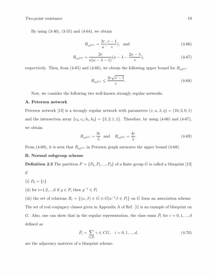
By using (3-46), (3-55) and (4-64), we obtain

Rαβ(1) =2r

κ(v − 1

v), and (4-66)

Rαβ(2) =2r

κ(κ− λ− 1)(κ− λ− 2κ− λ

v), (4-67)

respectively. Then, from (4-65) and (4-66), we obtain the following upper bound for Rαβ(1)

Rαβ(1) ≤ 2r√v − 1

v. (4-68)

Now, we consider the following two well-known strongly regular networks.

A. Petersen network

Petersen network [13] is a strongly regular network with parameters (v, κ, λ, η) = (10, 3, 0, 1)

and the intersection array {c0, c1; b1, b2} = {3, 2; 1, 1}. Therefore, by using (4-66) and (4-67),

we obtain

Rαβ(1) =3r

5and Rαβ(2) =

4r

5. (4-69)

From (4-69), it is seen that Rαβ(1) in Petersen graph saturates the upper bound (4-68).

B. Normal subgroup scheme

Definition 2.3 The partition P = {P0, P1, ..., Pd} of a finite group G is called a blueprint [13]

if

(i) P0 = {e}

(ii) for i=1,2,...,d if g ∈ Pi then g−1 ∈ Pi

(iii) the set of relations Ri = {(α, β) ∈ G ⊗ G|α−1β ∈ Pi} on G form an association scheme.

The set of real conjugacy classes given in Appendix A of Ref. [1] is an example of blueprint on

G. Also, one can show that in the regular representation, the class sums Pi for i = 0, 1, ..., d

defined as

Pi =∑

γ∈Pi

γ ∈ CG, i = 0, 1, ..., d, (4-70)

are the adjacency matrices of a blueprint scheme.


In [1], it has been shown that, if H be a normal subgroup of G, the following blueprint

classes

P0 = {e}, P1 = G− {H}, P2 = H − {e}, (4-71)

define a strongly regular network with parameters (v, κ, λ, η) = (g, g − h, g − 2h, g − h) and

the following intersection array

{c0, c1; b1, b2} = {g − h, h− 1; 1, g − h}, (4-72)

where, g := |G| and h := |H|. It is interesting to note that in normal subgroup scheme,

the intersections numbers and other parameters depend only on the cardinalities of the group

and its normal subgroup. By using (2-13), the QD parameters are given by {α1, α2;ω1, ω2} =

{g − 2h, 0; g − h, (g − h)(h− 1)}. Also, from (4-71), it is seen that |Γ2(α)| = h− 1. Then, by

using (4-66) and (4-67), we obtain

Rαβ(1) =2r(g − 1)

g(g − h), and Rαβ(2) =

2r

(g − h). (4-73)

One should notice that, the maximum degree κ for normal subgroup scheme is κmax = g−2

(h = 2), which can be appear in networks with even cardinality such as dihedral group.

Therefore, for normal subgroup scheme (strongly regular networks with parameters (g, g −

h, g − 2h, g − h)), we have

κ ≤ g − 2, (4-74)

and therefore, by using (4-65), (4-78) and (4-75) (κ = g − h), we obtain upper and lower

bounds for Rαβ(1) and Rαβ(2) as follows

2r(g − 1)

g(g − 2)≤ Rαβ(1) ≤ 2r

√g − 1

g,

2r

g − 2≤ Rαβ(2) ≤ 2r√

g − 1. (4-75)

As an example, we consider the dihedral group G = D2m, where its normal subgroup is

H = Zm. Therefore, the blueprint classes are given by

P0 = {e}, P1 = {b, ab, a2b, ..., am−1b}, P2 = {a, a2, ..., a(m−1}, (4-76)


which form a strongly regular network with parameters (2m,m, 0, m) and the following inter-

section array

{c0, c1; b1, b2} = {m,m− 1; 1, m}. (4-77)

By using (4-78), we obtain

Rαβ(1) =r(2m− 1)

m2, and Rαβ(2) =

2r

m. (4-78)

4.3 Cycle network Cv

A cycle network or cycle is a network that consists of some number of vertices connected in

a closed chain. The cycle network with v vertices is denoted by Cv with κ = 2. For odd

v = 2m+ 1, the intersection array is given by

{c0, ..., cm; b1, ..., bm} = {2, 1, ..., 1; 1, ..., 1, 1}, (4-79)

where, for even v = 2m, we have

{c0, ..., cm; b1, ..., bm} = {2, 1, ..., 1, 2; 1, ..., 1, 2} (4-80)

and the network consists of m + 1 strata. We consider v = 2m (the case v = 2m + 1 can be

considered similarly). Then, by using the recursion relations (2-22) and (2-24) one can obtain

the following closed form for the Stieltjes function

Gµ(x) =1

m

T ′m(x/2)

Tm(x/2), (4-81)

where, Tk(x) are Tchebyshev polynomials of the first kind.

By using (3-46), (3-55) and (3-61) we obtain

Rαβ(1) = r(2m− 1

2m), Rαβ(2) = 2r(

m− 1

m), and Rαβ(3) = 3r(

2m− 3

2m), (4-82)

respectively. From (4-82), one can easily deduce that

Rαβ(k) = kr(2m− k

2m) k = 1, 2, ..., m. (4-83)


At the limit of the large m, the cycle network tend to the infinite line network and the

Stieltjes function (4-81) reads as

Gµ(x) =1√

x2 − 4. (4-84)

Then, for A0 we have

A0 = limx→2

((x− 2)Gµ(x)) = 0. (4-85)

Therefore, by using (3-46), (3-55) and (3-61) we obtain

Rαβ(1) = r, Rαβ(2) = 2r, Rαβ(3) = 3r. (4-86)

In fact, it can be easily shown that

Rαβ(k) = kr, k = 1, 2, ... (4-87)

where, this result could be obtained from (4-83), for large m.

As (4-83) indicates, for m larger than ∼ 70 the difference |Rαβ(k) − kr| is equal to ∼ 0.01,

where for m larger than ∼ 100 we have |Rαβ(k) −kr| ∼ 0. Therefore, the finite resistor network

C2m, with m ∼ 100 is a good approximation for the infinite line resistor network.

4.4 d-cube

The d-cube, i.e. the hypercube of dimension d, also called Hamming cubes, is a network with

2d nodes, each of which can be labeled by an d-bit binary string. Two nodes on the hypercube

described by bitstrings ~x and ~y are are connected by an edge if |~x − ~y| = 1, where |~x| is the

Hamming weight of ~x. In other words, if ~x and ~y differ by only a single bit flip, then the two

corresponding nodes on the graph are connected. Thus, each of the 2d nodes on the d-cube

has degree d. For the d-cube we have d+ 1 strata with

κi =d!

i!(d− i)!, 0 ≤ i ≤ d− 1. (4-88)


The intersection numbers are given by

bi = d− i, 0 ≤ i ≤ d− 1; ci = i, 1 ≤ i ≤ d. (4-89)

Then, by using (3-46), (3-55) and (3-61), we obtain

Rαβ(1) =2d − 1

d2d−1r, Rαβ(2) =

2d−1 − 1

(d− 1)2d−2r, and

Rαβ(3) =r

d(d− 1)(d− 2){2

d(d2 − 2d+ 2)− 3d(d− 1)− 2

2d−1}. (4-90)

From (4-90) one can see that, at the limit of the large dimension d, the two-point resistances

Rαβ(i) , i = 1, 2, 3 tend to zero. Since Rαβ(1) tend to zero for d larger than ∼ 200. Therefore,

the finite d-cube with d larger than ∼ 200 is a good approximation for the infinite hypercube

resistor network.

4.5 Johnson network

Let n ≥ 2 and d ≤ n/2. The Johnson network J(n, d) has all d-element subsets of {1, 2, ..., n}

such that two d-element subsets are adjacent if their intersection has size d−1. Two d-element

subsets are then at distance i if and only if they have exactly d− i elements in common. The

Johnson network J(n, d) has v = n!d!(n−d)!

vertices, diameter d and the valency κ = d(n − d).

Its intersection array is given by

bi = (d− i)(n− d− i), 0 ≤ i ≤ d− 1; ci = i2, 1 ≤ i ≤ d, (4-91)

Then, by using (3-46), (3-55) and (3-61), we obtain

Rαβ(1) =2(n!− d!(n− d)!)

d(n− d)n!r,

Rαβ(2) =2r

d(d− 1)(n− d)(n− d− 1){d(n−d)− (n−2)+

d!(n− d)!(n− 2− 2d(n− d))

n!} and

Rαβ(3) =2r

d(d− 1)(d− 2)(n− d)(n− d− 1)(n− d− 2){d2(n− 2d+ 1)+


(3n−2d(n−d)−10)d(n− d)d!(n− d)!

n!+ [d2(n−d)2−d(n−d)(3n−9)−4(d−1)(n−d−1)+

2(n− 2)(n− 4)](1− d!(n− d)!

n!)}. (4-92)

It could be noticed that for a give d, the result (4-92) show that, at the limit of the large

dimension n, the two-point resistances Rαβ(i) , i = 1, 2, 3 tend to zero. Since Rαβ(1) tend to

zero for n larger than ∼ 200. Therefore, the finite Johnson network J(n, d) with n larger than

∼ 200 is a good approximation for the infinite Johnson resistor network.

5 Two-point resistances in more general networks

Although, we discussed through the paper only the case of distance-regular networks, but

also the method can be used for any arbitrary regular network. For calculating two-point

resistances, we need only to know the Stieltjes function Gµ(x). For two arbitrary nodes α and

β of the network, we choose one of the nodes, say α, as reference vertex. Then, the Stieltjes

function Gµ(x) can be calculated by using the recursion relations (2-22) and (2-24), where, as

it has be shown in [20], the coefficients αi and βi, for i = 1, ..., d in the recursion relations are

obtained by applying the Lanczos algorithm to the adjacency matrix of the network and the

reference vertex |α〉. In fact, the adjacency matrix of the network takes a tridiagonal form in

the orthonormal basis {|φi〉, i = 0, 1, ..., d} produced by Lanczos algorithm and so we obtain

again three term recursion relations as (2-22). But, in general, the basis produced by Lanczos

algorithm do not define a stratification basis, in the sense that, a vertex ket |β〉 of the network

may be appear in more than one of the base vectors |φi〉. In these cases, if d is equal to

v (the number of vertices of the network), one can write each vertex ket |β〉 uniquely as a

superposition of the base vectors |φi〉 and calculate two-point resistance Rαβ by calculating

the entries 〈φi|L−1|α〉 for all i = 0, 1, ..., d as illustrated through the paper. In the most cases,

d is less than v. In these cases, we need to obtain some additional orthonormal base vectors

{|ψi〉, i = 1, .., v − d − 1} such that the new bases are orthogonal to the subspace spanned


by {|φi〉, i = 0, 1, ..., d}. One can obtain some such additional base vectors, by choosing

a normalized vector orthogonal to the subspace spanned by {|φi〉, i = 0, 1, ..., d} as a new

reference state and applying the Lanczos algorithm to the adjacency matrix of the network

and the new reference state. If the number of the new orthonormal base vectors still be less

than v−d−1, we choose another normalized reference state orthogonal to the subspace spanned

by all previous orthonormal bases and apply the Lanczos algorithm to the adjacency matrix

and the new chosen reference state. By repeating this process until to obtain v orthonormal

basis, one can solve a system of v equations with v unknowns to write each vertex ket β as

superposition of the v orthonormal bases.

6 Conclusion

The resistance between two arbitrary nodes in a distance-regular resistor network was obtained

in terms of the Stieltjes transform of the spectral measure or Stieltjes function associated with

the network and its derivatives. It was shown that the resistances between a node α and all

nodes β belonging to the same stratum with respect to the α are the same. Also, explicit an-

alytical formulaes for two-point resistances Rαβ for β belonging to the first, second and third

stratum with respect to the α were driven in terms of the size of the network and the corre-

sponding intersection numbers. In particular, the two-point resistances in a strongly regular

network with parameters (v, κ, λ, µ) were given in terms of these parameters. Moreover, the

lower and upper bounds for two-point resistances in strongly regular networks was discussed. It

was discussed that, the introduced method can be used not only for distance-regular networks,

but also for any arbitrary regular network by employing the Lanczos algorithm iteratively.


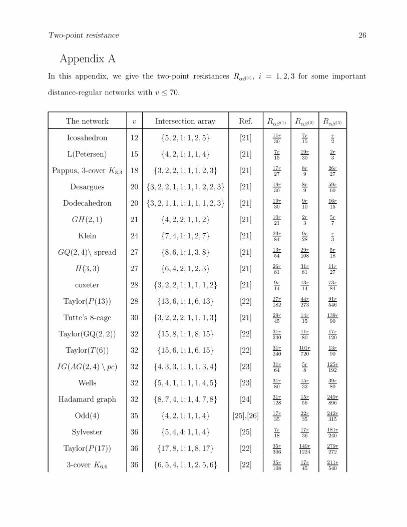
Appendix A

In this appendix, we give the two-point resistances Rαβ(i) , i = 1, 2, 3 for some important

distance-regular networks with v ≤ 70.

The network v Intersection array Ref. Rαβ(1) Rαβ(2) Rαβ(3)

Icosahedron 12 {5, 2, 1; 1, 2, 5} [21] 11r30

7r15

r2

L(Petersen) 15 {4, 2, 1; 1, 1, 4} [21] 7r15

19r30

2r3

Pappus, 3-cover K3,3 18 {3, 2, 2, 1; 1, 1, 2, 3} [21] 17r27

8r9

26r27

Desargues 20 {3, 2, 2, 1, 1; 1, 1, 2, 2, 3} [21] 19r30

8r9

59r60

Dodecahedron 20 {3, 2, 1, 1, 1; 1, 1, 1, 2, 3} [21] 19r30

9r10

16r15

GH(2, 1) 21 {4, 2, 2; 1, 1, 2} [21] 10r21

2r3

5r7

Klein 24 {7, 4, 1; 1, 2, 7} [21] 23r84

9r28

r3

GQ(2, 4)\ spread 27 {8, 6, 1; 1, 3, 8} [21] 13r54

29r108

5r18

H(3, 3) 27 {6, 4, 2; 1, 2, 3} [21] 26r81

31r81

11r27

coxeter 28 {3, 2, 2, 1; 1, 1, 1, 2} [21] 9r14

13r14

73r84

Taylor(P (13)) 28 {13, 6, 1; 1, 6, 13} [22] 27r182

44r273

91r546

Tutte’s 8-cage 30 {3, 2, 2, 2; 1, 1, 1, 3} [21] 29r45

14r15

139r90

Taylor(GQ(2, 2)) 32 {15, 8, 1; 1, 8, 15} [22] 31r240

11r80

17r120

Taylor(T (6)) 32 {15, 6, 1; 1, 6, 15} [22] 31r240

101r720

13r90

IG(AG(2, 4) \ pc) 32 {4, 3, 3, 1; 1, 1, 3, 4} [23] 31r64

5r8

125r192

Wells 32 {5, 4, 1, 1; 1, 1, 4, 5} [23] 31r80

15r32

39r80

Hadamard graph 32 {8, 7, 4, 1; 1, 4, 7, 8} [24] 31r128

15r56

249r896

Odd(4) 35 {4, 2, 1; 1, 1, 4} [25],[26] 17r35

22r35

242r315

Sylvester 36 {5, 4, 4; 1, 1, 4} [25] 7r18

17r36

181r240

Taylor(P (17)) 36 {17, 8, 1; 1, 8, 17} [22] 35r306

149r1224

279r272

3-cover K6,6 36 {6, 5, 4, 1; 1, 2, 5, 6} [22] 35r108

17r45

211r540


The network v Intersection array Ref. Rαβ(1) Rαβ(2) Rαβ(3)

SRG\ spread 40 {9, 6, 1; 1, 2, 9} [27] 13r60

11r45

r4

Ho− Si2(x) 42 {16, 5, 1; 1, 1, 6} [25] 41r126

8r21

34r105

Mathon (Cycl(13, 3)) 42 {13, 8, 1; 1, 4, 13} [28] 41r273

89r546

91r13

GO(2, 1) 45 {4, 2, 2, 2; 1, 1, 1, 2} [23] 22r45

32r45

4r5

3-cover GQ(2, 2) 45 {6, 4, 2, 1; 1, 1, 4, 6} [23] 44r135

107r270

221r540

Hadamard graph 48 {12, 11, 6, 1; 1, 6, 11, 12} [22] 47r288

23r132

565r3168

IG(AG(2, 5) \ pc) 50 {5, 4, 4, 1; 1, 1, 4, 5} [23] 49r125

12r25

123r250

Mathon (Cycl(16, 3)) 51 {16, 10, 1; 1, 5, 16} [28] 25r204

89r680

68r510

GH(3, 1) 52 {6, 3, 3; 1, 1, 2} [29] 51r156

11r26

23r52

Taylor(SRG(25, 12)) 52 {25, 12, 1; 1, 12, 25} [22] 51r650

319r3900

13r156

3-cover K9,9 54 {9, 8, 6, 1; 1, 3, 8, 9} [22] 53r243

13r54

239r972

Gosset,Tayl(Schlafli) 56 {27, 10, 1; 1, 10, 27} [22] 55r756

289r3780

49r630

Taylor(Co-Schlafli) 56 {27, 16, 1; 1, 16, 27} [22] 55r756

227r3024

11r144

Perkel 57 {6, 5, 2; 1, 1, 3} [25],[30] 56r171

22r57

68r171

Mathon(Cycl(11, 5)) 60 {11, 8, 1; 1, 2, 11} [28] 59r330

32r165

r5

Mathon(Cycl(19, 3)) 60 {19, 12, 1; 1, 6, 19} [28] 59r570

187r1710

3151r570

Taylor(SRG(29, 14)) 60 {29, 14, 1; 1, 14, 29} [22] 59r870

214r3045

29r406

GH(2, 2) 63 {6, 4, 4; 1, 1, 3} [29] 62r189

76r189

271r504

H(3, 4),Doob 64 {9, 6, 3; 1, 2, 3} [22] 7r32

r4

25r96

Locally Petersen 65 {10, 6, 4; 1, 2, 5} 64r325

73r325

49r156

Doro 68 {12, 10, 3; 1, 3, 8} 67r408

145r816

253r1020

Doubled Odd(4) 70 {4,3,3,2,2,1,1; 1,1,2,2,3,3,4} [22] 69r140

68r105

869r1260

J(8, 4) 70 {16, 9, 4, 1; 1, 4, 9, 16} [22] 69r560

337r2520

691r5040


References

[1] M. A. Jafarizadeh and S. Salimi, J. Phys. A : Math. Gen. 39, 1-29 (2006)

[2] J. Cserti, Am. J. Phys. 68, 896 (2000)(Preprint cond-mat/9909120).

[3] P. G. Doyle and J. L. Snell, RandomWalks and Electric Networks (The Carus Mathemat-

icalMonograph series 22) (Washington, DC: The Mathematical Association of America))

pp 83149 (Preprint math.PR/0001057)(1984)

[4] B. van der Pol, The finite-difference analogy of the periodic wave equation and the po-

tential equation Probability and Related Topics in Physical Sciences (Lectures in Applied

Mathematics vol 1) ed M Kac (London: Interscience) pp 23757 (1959)

[5] S. Katsura, T. Morita, S. Inawashiro, T. Horiguchi and Y. Abe, Lattice Greens function:

introduction J. Math. Phys. 12, 8925 (1971)

[6] D. R. Hofstadter, Phys. Rev. B 14, 2239 (1976).

[7] M.I. Molina, Phys. Rev. B 73, 014204 (2006).

[8] B. Kyung, S. S. Kancharla, D. Snchal, and A.-M. S. Tremblay, M. Civelli and G. Kotliar,

Phys. Rev. B 73, 165114 (2006)

[9] S. B Wilkins et al., Phys. Rev. B 73, 060406 (R) (2006)

[10] J.Cserti J, G. David and P. Attila, Am. J. Phys. 70, 1539 (2002)

[11] G. Kirchhoff, Phys. Chem. 72 497508 (1847)

[12] F. Y. Wu, J. Phys. A: Math. Gen. 37, 6653 (2004).

[13] R. A. Bailey, Association Schemes: Designed Experiments, Algebra and Combinatorics (

Cambridge University Press, Cambridge, 2004).


[14] E. Bannai and T. Ito, Algebraic Combinatorics I: Association schemes, Ben-

jamin/Cummings, London (1984).

[15] J. A. Shohat, and J. D. Tamarkin, The Problem of Moments, American Mathematical

Society, Providence, RI (1943).

[16] A. Hora, and N. Obata, Fundamental Problems in Quantum Physics, World Scientific,

284(2003).

[17] T. S. Chihara (1978), An Introduction to Orthogonal Polynomials, Gordon and Breach,

Science Publishers Inc.

[18] A. Hora, and N. Obata, Quantum Information V, World Scientific, Singapore (2002).

[19] A. Hora and N. Obata, An Interacting Fock Space with Periodic Jacobi Parameter Ob-

tained from Regular Graphs in Large Scale Limit, to appear in: Quantum Information V,

Hida, T., and Saito , K., Ed., World Scientific, Singapore (2002).

[20] M. A. Jafarizadeh, S. Salimi and R. Sufiani, e-print quan-ph/0606241.

[21] W. H. Haemers, E. Spence, Linear and Multilinear Algebra 39, 91-107 (1995)

[22] E. R. van Dam, W. H. Haemers, J. H. Koolen and E. Spence, Journal of combinatorial

theory, Series A 113, 1805-1820 (2006)

[23] E. R. van Dam and W. H. Haemers, J. Algebraic Combin.15, 189-202 (2002)

[24] E. R. van Dam, Linear Algebra Appl. 396, 303-316 (2005)

[25] A. E. Brouwer and W. H. Haemers, European J. Combin. 14, 397-407(1993)

[26] T. Huang and C. Liu, Graphs Combin. 15,195-209 (1999)

[27] J. Degraer and K. Coolsaet, Discrete Math. 300, 71-81 (2005)


[28] R. Mathon, Congr. Numer. 13, 123-155 (1975)

[29] W. H. Haemers, Linear Algebra Appl. 236, 256-278 (1996)

[30] K. Coolsaet and J. Degraer, Des. Codes Cryptogr. 34, 155-171 (2005)

Calculating two-point resistances in distance-regular resistor ...

Documents

Transcript of Calculating two-point resistances in distance-regular resistor ...