
A Continuum Electrostatic Approach for Calculating ... - CORE
277
AC ONTINUUM E LECTROSTATIC A PPROACH FOR C ALCULATING T HE B INDING E NERGETICS OF M ULTIPLE L IGANDS DISSERTATION submitted to the Faculty of Biology, Chemistry and Geoscience of the University of Bayreuth, Germany for obtaining the degree of Doctor of Natural Sciences presented by Timm Essigke Bayreuth 2007
-
Upload
khangminh22 -
Category
Documents
-
view
1 -
download
0
Transcript of A Continuum Electrostatic Approach for Calculating ... - CORE

A CONTINUUM ELECTROSTATIC
APPROACH FOR CALCULATING THE
BINDING ENERGETICS OF MULTIPLE
LIGANDS
D I S S E R T A T I O N
submitted to
the Faculty of Biology, Chemistry and Geoscience
of the University of Bayreuth, Germany
for obtaining the degree of
Doctor of Natural Sciences
presented by
Timm Essigke
Bayreuth 2007


Die vorliegende Arbeit wurde in dem Zeitraum von Januar2004 bis Dezember 2007 an der Universitat Bayreuth unter derLeitung von Professor G. Matthias Ullmann erstellt.
Vollstandiger Abdruck der von der Fakultat Biologie, Chemieund Geowissenschaften der Universitat Bayreuth genehmigtenDissertation zur Erlangung des akademischen Grades Doktorder Naturwissenschaften (Dr. rer. nat.).
Erster Prufer: Prof. Dr. G. Matthias UllmannZweiter Prufer: Prof. Dr. Holger DobbekDritter Prufer: Prof. Dr. Thomas HellwegPrufungsvorsitz: Prof. Dr. Jurgen Senker
Tag der Einreichung: 20.12.2007Zulassung zur Promotion: 09.01.2008Annahme der Dissertation: 24.01.2008Auslage der Arbeit: 24.01.2008 - 06.02.2008Kolloquium: 20.02.2008

A CONTINUUM ELECTROSTATIC
APPROACH FOR CALCULATING THE
BINDING ENERGETICS OF MULTIPLE
LIGANDS


SUMMARY
Complex biomolecules like proteins or nucleic acids can transiently bind various ligands, e.g.,electrons, protons, ions or larger molecules. This property is the key to enzymatic catalysis,regulation and energy transduction in biological systems. Interactions between different lig-and binding sites can lead to complex titration behaviors, which can be explained based on amicrostate description of the system. Previous approaches to calculate the binding behavior ofmultiple ligand, only treated sites with one or no ligand bound by using a binary state vectorto describe the system. Also only one or two ligand types, i.e., protons or electrons, were usedfor the calculation.
In this thesis, I derive a more general formulation of the theory of ligand binding to biomole-cules. For each site any number of charge forms and rotamer forms are allowed as well asany number of ligands and any number of ligand types can be bound. Charge and rotamerforms of sites can be parameterized by measurements on model reactions in solution or byquantum chemical calculations. An energy function is described, consistently combiningexperimentally determined contributions and those, which can be calculated by continuumelectrostatics, molecular mechanics and quantum chemistry. Programs (i.e., QMPB and PerlMolecule) were developed to perform calculations based on the generalized ligand bindingtheory. The class library Perl Molecule was developed to write powerful Perl programs, whichperform the necessary processing steps, e.g., for the conversion of a pdb-file into the inputrequired for energy calculations. The generated input contains all experimentally determinedor molecular mechanically and quantum chemically obtained parameters. The energy calcu-lations are performed by the program QMPB, which uses other programs for the continuumelectrostatics calculations to solve the linearized Poisson-Boltzmann equation. The computa-tions scale linearly with the total number of sites of the system and can easily be performed inparallel. From the obtained energies, microscopic ligand binding probabilities can be calcu-lated as function of chemical potentials of ligands in solution, e.g., by a Monte Carlo program.Additionally, microscopic and macroscopic equilibrium constants can be computed.
The usefullness and correctness of the new approach based on a generalized ligand bind-ing theory is demonstrated by a number of studies on diverse examples. Because variousgroups used Lysozyme as benchmark system for continuum electrostatics, it is chosen totest if previously obtained results can be reproduced with QMPB. Different quantum chemicalapproaches are applied to the benzoquinone system for parameterizing a site with several pro-tonation and reduction forms. A complex site is also the CuB center in Cytochrome c oxidase,which is studied to decide if multiple protonation forms of the coordinating histidines are in-volved in the reaction mechanism. Factors influencing the reduction potential of the electrontransfer protein ferredoxin are analyzed using the programs Perl Molecule and QMPB. Here,
7

8 Summary
in particular conformational changes of a peptide bond in the vicinity of the [2Fe-2S] centerare of interest. The protonation form of a neighboring glutamate turns out to influence thereduction potential strongly. Protonation and phosphorylation studies on the protein HPrlead to the development of a four-microstate model to explain conformational changes on ahistidine, which can be observed by experiment, molecular dynamics simulation and elec-trostatic calculations. The phosphorylation and protonation state dependent conformationalchange can be related to the dual role of the protein in regulation and phosphate-transfer.The new microstate description does not only allow to analyze thermodynamic properties butalso paved the road for the study of the kinetics of charge transfer.

ZUSAMMENFASSUNG
Komplexe Biomolekule, wie Proteine oder Nukleinsauren, sind in der Lage, vorubergehendverschiedene Liganden zu binden, wie z. B. Elektronen, Protonen, Ionen oder großere Mo-lekule. Diese Eigenschaft ist der Schlussel zur enzymatischen Katalyse, zur Regulation undzur Energietransduktion in biologischen Systemen. Die Interaktionen verschiedener Ligan-denbindungsstellen konnen zu komplexem Titrationsverhalten fuhren, das basierend auf ei-ner Mikrozustandsbeschreibung des Systems erklart werden kann. Fruhere Ansatze, das Bin-dungsverhalten von mehreren Liganden zu berechnen, behandelten nur Bindungsstellen, dieentweder einen oder keinen Liganden gebunden hatten, so dass ein binarer Zustandsvektorzur Beschreibung des Systems benutzt werden konnte. Außerdem wurden nur ein oder zweiLigandentypen, wie z. B. Elektronen oder Protonen, fur die Rechnung zugelassen.
In der vorliegenden Arbeit leite ich eine generellere Formulierung der Ligandenbindungstheo-rie fur Biomolekule her. Fur jede Bindungsstelle sind eine beliebige Anzahl von Ladungs-und Rotamerformen moglich und es konnen eine beliebige Anzahl von Liganden und ei-ne beliebige Anzahl von Ligandentypen gebunden werden. Ladungs- und Rotamerformenvon Bindungsstellen konnen durch Messungen von Modellreaktionen in Losung oder durchquantenchemische Rechnungen parameterisiert werden. Eine Energiefunktion wird beschrie-ben, die experimentell bestimmte Beitrage, sowie Beitrage aus Kontinuumselektrostatik-,Molekularmechanik- und Quantenchemierechnungen konsistent kombiniert. Hierzu wurdenProgramme, insbesondere QMPB und Perl Molecule, entwickelt, die es ermoglichen, Berech-nungen basierend auf der generalisierten Ligandenbindungstheorie durchzufuhren. Die Klas-senbibliothek Perl Molecule wurde entwickelt, die es erlaubt, leistungsfahige Perl-Programmezu schreiben. Diese Programme fuhren die Schritte durch, die notwendig sind, um z. B. ei-ne PDB-Datei in die fur Energieberechnungen benotigten Eingabe-Dateien umzuwandeln. Dieso erzeugten Eingabe-Dateien enthalten alle Parameter, die entweder experimentell bestimmtoder uber Molekularmechanik- und Quantenchemierechnungen ermittelt wurden. Die Ener-gieberechnungen werden von dem Programm QMPB durchgefuhrt, das andere Programmefur die Kontinuumselektrostatik-Rechnungen benutzt, die die linearisierte Poisson-BoltzmannGleichung losen. Die mit QMPB durchgefuhrten Rechnungen skalieren linear mit der totalenAnzahl von Bindungsstellen des Systems und konnen einfach parallel ausgefuhrt werden. Vonden ermittelten Energien konnen, z. B. mit Hilfe eines Monte Carlo Programmes, mikrosko-pische Wahrscheinlichkeiten fur die Ligandenbindung errechnet werden. Diese Wahrschein-lichkeiten sind abhangig von den chemischen Potentialen der Liganden in Losung. Zusatzlichkonnen mikroskopische und makroskopische Gleichgewichtskonstanten berechnet werden.
Der Nutzen und die Richtigkeit des hier beschriebenen neuen Ansatzes, basierend auf ei-ner allgemeineren Ligandenbindungstheorie, wird anhand von einigen Untersuchungen an
9

10 Zusammenfassung
einer Reihe von Beispielen demonstriert. Da schon verschiedene Gruppen Lysozym als Test-system fur Kontinuumselektrostatikrechnungen genutzt haben, wird es auch in der vorliegen-den Arbeit verwendet, um die Reproduzierbarkeit alterer Ergebnisse mit QMPB zu uberprufen.Unterschiedliche quantenchemische Methoden wurden auf das Benzochinon-System zur Pa-rameterisierung als Bindungsstelle mit mehreren Protonierungs- und Reduktionsformen an-gewendet. Eine komplizierte Bindungsstelle stellt auch das CuB Zentrum von Cytochrom cOxidase dar. Es wird untersucht, ob mehrere Protonierungsformen der koordinierenden Hi-stidine am Reaktionsmechanismus beteiligt sind. Mit den Programmen Perl Molecule undQMPB werden Faktoren analysiert, die das Reduktionspotential des Elektronenubertrager-Proteins Ferredoxin beeinflussen. In diesem Zusammenhang sind besonders konformationel-le Anderungen einer Peptidbindung in der Nahe des [2Fe-2S] Zentrums von Interesse. Eshat sich herausgestellt, dass die Protonierungsform eines benachbarten Glutamates einengrossen Einfluss auf das Reduktionspotential hat. Untersuchungen der Protonierung undPhosphorylierung des Proteins HPr fuhren zur Entwicklung eines Vierzustandsmodells. Damitkonnen konformationelle Anderungen eines Histdins erklart werden, die experimentell, in Mo-lekulardynamiksimulationen und in Elektrostatikrechnungen beobachtet werden konnen. Dievom Phosphorylierungs- und Protonierungszustand abhangigen konformationellen Anderungenkonnen mit den zwei Aufgaben des Proteins in der Regulation und im Phosphattransfer in Ver-bindung gebracht werden. Die neue Mikrozustandsbeschreibung erlaubt es nicht nur, ther-modynamische Eigenschaften zu analysieren, sondern bereitet auch den Weg fur kinetischeUntersuchungen von Ladungstransfers.

PREFACE
Acknowledgements
This thesis was done in the last four years in the group of Professor G. Matthias Ullmannat the University of Bayreuth. Matthias has been a friend and mentor for almost the last10 years. After raising my interest in computational biochemistry and biophysics, he con-tinuously supported me as undergraduate student at Free University Berlin and The ScrippsResearch Institute, La Jolla, USA, as researcher in Rebecca Wade’s group in Heidelberg and ashis graduate student here in Bayreuth in the last years. I am particularly grateful to Matthiasfor also sticking by me in difficult times. His contribution of countless ideas, suggestions andadvice was so valueable to my work, that I can not thank him enough. I am also grateful forhis contribution of the programs SMT and GMCT to the toolchain developed in this thesis. Heprovided me with excellent working conditions and substantial computation time, which wasimportant for many applications.
Eva-Maria Krammer tremendously helped during my work. She was the first to test my pro-grams Perl Molecule and QMPB by herself on the bacterial photosynthetic reaction center.On one hand, the complex system challenged my programs, previously only tested on muchsmaller proteins, and on the other hand using the programs without having in mind howthey work in detail highlighted several bugs and pitfalls which could then be removed. Manysuggestions of her helped to improve the programs. Our aim to parameterize ubiquinonefor the reaction center led to a broad study of quantum chemical methods applied to benzo-quinone, duroquinone and ubiquinone. Eva conducted an intense literature research and rannumerous Gaussian calculations of which I can only discuss a small fraction in the applica-tion section of this work. I am very grateful to her for proofreading my thesis and the manysuggestions and corrections she made. Eva’s encouragements and exemplary diligence werea great motivation.
With Thomas Ullmann I had many valueable discussions profitting from his detailed literatureknowledge, his insights obtained from running countless calculations with MEAD and ADFand his studies of the source code of these programs to extend them. In many respects heis picking up and extending my work. For example he does studies with sidechain rotamersusing QMPB which are much more advanced than my initial tests. Thomas implemented asophisticated membrane model into MEAD, which allows to study membrane proteins in avery realistic environment including membrane potentials. To use the new helper programsfor solving the Poisson-Boltzmann equation only little changes in a script generated by QMPBwere required. I am also thankful for his good company at our core hours during night shift.
11

12 Preface
With Punnagai Munusami I was collaborating to test and use Perl Molecule and QMPB onher system Cytochrome c oxidase. A part of this work is reported in the applications section.Punnagai is clearly our Gaussian expert and contributed many helpful suggestions to thequinone project of Eva and me. I appreciated the many discussions we had.
Mirco Till is using QMPB to calculate microstate energies as basis for kinetic studies withDMC. Therefore, his work builds up on mine and extends it into a new direction. The appli-cation on gramicidin A is briefly discussed and other applications, e.g., on the reaction centerwith Eva will follow. I am grateful, that he backed me up in case of computer and networkproblems. Redundancy is particularly important on OSI layer 8. I enjoyed our computer andprogramming related discussions.
All the other present and former group members also had their contributions adding theirscientific skills and making every day more fun: Dr. Elisa Bombarda brought a lot of vi-tality into our sometime too quite group. She did the groundwork for including membranepotentials into electrostatic computations as it was implemented by Thomas for QMPB. FrankDickert was always helpful with his superb technical skills and a driving force for most groupactivities. He provided the protein of his diploma project, cytochrome c2, as my second testcase for QMPB after lysozyme. Edda Kloppmann saved me a lot of work providing the LATEXstyle files for this document. In the last months I miss our discussions. Dr. Torsten Beckerwas always a pleasant office mate, helping with his physical knowledge, intuition and humor.The program DMC, he develops together with Mirco, is breaking new ground in simulatinglong range charge transfer. Dr. Astrid Klingen’s study on the histidine treatment procedurein Multiflex was helpful for a better comparison. Supervising the bachelor thesis of ThomasWeinmaier was an instructive experience. I am grateful for his work creating a SWIG interfacefor MEAD and his suggestions of a number of informatics books. I thank Siriporn Promsri forthe clock (Fig. 4.6) stimulating some good ideas. I miss the discussions about ferredoxin, itsreductase and other topics with Veronica Dumit and I am looking forward to her joining ourgroup again. I am happy, that Silke Wieninger is the first member of a new generation of PhDstudents in our group, who will solve all the remaining problems.
Not only inside the group my thesis was supported by a number of inspiring collaborations,but we also had a very fruitful collaboration with Nadine Homeyer and Professor HeinrichSticht (University of Erlangen) on the regulatory and phosphate transfer protein HPr. Researchwas a perfect team play, where results of one group guided the next steps of the other group.I very much enjoyed our constructive and motivating discussions.
Thanks to Sabrina Fortsch and Alexander Dotor for proofreading and making helpful sugges-tions on the informatics chapter.
I would not have come to this point without Professor Ernst-Walter Knapp (Free UniversityBerlin) supporting me during my studies and guiding me into this interesting field of research.Likewise I am deeply grateful for Dr. Rebecca Wade’s (EML Research gGmbH) support anddiscussions during my time in Heidelberg. The research I did with her on ferredoxin andother proteins highlighted shortcomings of previous programs. Therefore, it was the startingpoint for my thesis work.
My thesis substantially builds up on theoretical works of Professor Donald Bashford and hisgroup. His MEAD library was the basis for electrostatic programs I developed to be run byQMPB. I am thankful, that he realized even before the “open source revolution” that scientific

Preface 13
progress requires liberal licenses like the GPL, which allow that code is distributed and ex-tended free of charge for everyone on the internet. Professor Louis Noodleman and his groupdid pioneering work on combining quantum chemical and Poisson-Boltzmann calculations,which formed a good basis for my studies.
I acknowledge the progress ADF has made in the last years in particular in terms of speedand scaleability. I am grateful to Dr. Stan van Gisbergen for providing us with this superbsoftware package. I appreciate very much the work of the CHARMM and Gaussian developers,who’s programs were of great value during this work. Special thanks also to Dr. NicolasCalimet for writing and providing Hwire for hydrogen placement and to the developers of VMDfor molecular visualization. Several figures in this work were made with VMD, sometimesin combination with povray. Other figures were drawn with xfig, xmgrace, dia, inkscapeand chemtool. Typesetting was done with LATEX using Kile, KBibTex, KBib and Kpdf. Mostprogramming I did in Perl. I deeply appreciate the great work Dr. Larry Wall and many Perldevelopers contributing by CPAN packages to this work. Alike I acknowledge the work of thedevelopers of C++ and the GNU compiler. I appreciated doing all my work on Linux, deeplygrateful to Dr. Linus Torvalds and to many other kernel developers, the GNU Foundationand the Debian project for their great distribution. It was fun and a pleasant distraction toresearch which features this operation system can provide for us. It is impossible to thank allopen source developers for their programs explicitly which were helpful for my thesis.
I acknowledge the support of the compute center of the University of Bayreuth, in particularI thank Dr. Bernhard Winkler for running our compute cluster and backup.
Last but not least, I want to deeply thank my parents Jutta and Walter Essigke for theircontinuous support and encouragement. They gave me the freedom to choose my way andfollow my interests but never failing to be on my side if I needed their advice.

14 Preface
Typesetting Conventions
Italics are used for:
• Expressions in other languages than English (e.g., i.e., etc.)
• Organisms (Bacillus subtilis, Escherichia coli, E. coli)
• Equation symbols (∆∆GBorn, 〈xi(lm, {µλ})〉)
Constant width is used for:
• Class, object, method or attribute names
• Words taken from input and output files
Sans serif is used for:
• Program names (QMPB. Perl Molecule, Multiflex)

Preface 15
Publications
1. What Determines the Redox Potential of Ferredoxins?Timm Essigke, G. Matthias Ullmann, Rebecca C. WadeIn: Proceedings of the 13th International Conference on Cytochromes P450, MonduzziEditore, Bologna: 25-30, 2003
2. Calculation of the Redox Potential of Iron-Sulfur ProteinsTimm Essigke, Rebecca C. Wade and G. Matthias UllmannJ. Inorg. Biochem., 96(1),127, 2003
3. Formation and Characterization of an All-Ferrous Rieske Cluster and Stabilization of the[2Fe− 2S]0 Core by ProtonationEllen J. Leggate, Eckhard Bill, Timm Essigke, G. Matthias Ullmann and Judy HirstProc. Natl. Acad. Sci. USA, 101(30), 10913-10918, 2004
4. Effect of HPr Phosphorylation on Structure, Dynamics, and Interactions in the Course ofTranscriptional ControlNadine Homeyer, Timm Essigke, Heike Meiselbach, G. Matthias Ullmann and HeinrichStichtJ. Mol. Model., 13(3), 431-444, 2007
5. Effects of Histidine Protonation and Phosphorylation on Histidine-Containing Phospho-carrier Protein Structure, Dynamics, and Physicochemical PropertiesNadine Homeyer1, Timm Essigke1, G. Matthias Ullmann and Heinrich StichtBiochemistry, 46(43), 12314-12326, 2007
6. Investigating the Mechanisms of Photosynthetic Proteins Using Continuum Electrostat-icsG. Matthias Ullmann, Edda Kloppmann, Timm Essigke, Eva-Maria Krammer, Astrid R.Klingen, Torsten Becker, Elisa BombardaSubmitted to Photosyn. Res., 2007
7. Does Deprotonation of CuB Ligands Play a Role in the Reaction Mechanism of Cy-tochrome c Oxidase?M. Punnagai, Timm Essigke, and G. Matthias UllmannSubmitted to J. Am. Chem. Soc., 2007
8. Simulating the Proton Transfer in Gramicidin A by a Sequential Dynamical Monte CarloMethodMirco S. Till, Torsten Becker, Timm Essigke, and G. Matthias UllmannIn preparation for J. Phys. Chem., 2007
1Authors equally contributed

16

CONTENTS
Summary 7
Zusammenfassung 9
Preface 11
Acknowledgements . . . . . . . . . . . . . . . . . . . . . . . . . . . . . . . . . . . . . . . 11
Typing Conventions . . . . . . . . . . . . . . . . . . . . . . . . . . . . . . . . . . . . . . . 14
Publications . . . . . . . . . . . . . . . . . . . . . . . . . . . . . . . . . . . . . . . . . . . 15
1 Introduction 23
1.1 Techniques of Biomolecular Simulation . . . . . . . . . . . . . . . . . . . . . . . . 24
1.1.1 Molecular Mechanics . . . . . . . . . . . . . . . . . . . . . . . . . . . . . . . 24
1.1.2 Quantum Chemistry . . . . . . . . . . . . . . . . . . . . . . . . . . . . . . . . 25
1.1.3 Continuum Electrostatics . . . . . . . . . . . . . . . . . . . . . . . . . . . . . 25
1.2 Programs for Ligand Binding Studies . . . . . . . . . . . . . . . . . . . . . . . . . . 26
1.3 Aim of this Work . . . . . . . . . . . . . . . . . . . . . . . . . . . . . . . . . . . . . . 27
1.4 Outline of the Thesis . . . . . . . . . . . . . . . . . . . . . . . . . . . . . . . . . . . 28
2 Concepts and Theoretical Methods for Calculations of Ligand Binding Energetics 31
2.1 Concepts of Ligand Binding Reactions . . . . . . . . . . . . . . . . . . . . . . . . . 32
2.1.1 Microscopic and Macroscopic Equilibrium Constants . . . . . . . . . . . . 32
2.1.2 Chemical Potential and the Progress of a Chemical Reaction . . . . . . . . 35
2.1.3 Microstate Energy, Binding Free Energy and Reaction Free Energy . . . . 36
2.1.4 The Protonation Reaction . . . . . . . . . . . . . . . . . . . . . . . . . . . . . 38
2.1.5 The Reduction Reaction . . . . . . . . . . . . . . . . . . . . . . . . . . . . . . 39
2.2 Continuum Electrostatics . . . . . . . . . . . . . . . . . . . . . . . . . . . . . . . . . 41
2.2.1 The First Maxwell Equation . . . . . . . . . . . . . . . . . . . . . . . . . . . . 41
2.2.2 The Coulomb Equation . . . . . . . . . . . . . . . . . . . . . . . . . . . . . . 42
17

18 Contents
2.2.3 The Poisson Equation . . . . . . . . . . . . . . . . . . . . . . . . . . . . . . . 43
2.2.4 The Poisson-Boltzmann Equation . . . . . . . . . . . . . . . . . . . . . . . . 44
2.2.5 The Linearized Poisson-Boltzmann Equation . . . . . . . . . . . . . . . . . . 45
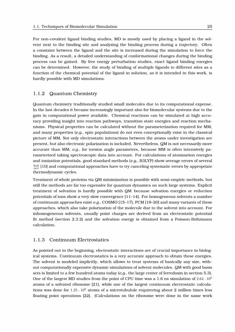
2.2.6 Solving the LPBE Numerically . . . . . . . . . . . . . . . . . . . . . . . . . . 45
2.3 Quantum Chemistry . . . . . . . . . . . . . . . . . . . . . . . . . . . . . . . . . . . . 51
2.3.1 Introduction to Density Functional Theory . . . . . . . . . . . . . . . . . . . 52
2.3.2 Charge Fitting . . . . . . . . . . . . . . . . . . . . . . . . . . . . . . . . . . . 55
2.4 Molecular Modeling . . . . . . . . . . . . . . . . . . . . . . . . . . . . . . . . . . . . 56
2.4.1 Molecular Mechanics . . . . . . . . . . . . . . . . . . . . . . . . . . . . . . . 56
2.4.2 Database Derived Force Fields or Statistical Potentials . . . . . . . . . . . . 58
2.4.3 Geometrical considerations . . . . . . . . . . . . . . . . . . . . . . . . . . . . 60
2.5 Summary . . . . . . . . . . . . . . . . . . . . . . . . . . . . . . . . . . . . . . . . . . 62
3 A Generalized Theory for Calculations of Ligand Binding Energetics 63
3.1 Towards an Energy Function for Ligand Binding . . . . . . . . . . . . . . . . . . . 64
3.1.1 The Grand Canonical Partition Function . . . . . . . . . . . . . . . . . . . . 64
3.1.2 The Microstate Energy Function . . . . . . . . . . . . . . . . . . . . . . . . . 65
3.1.3 Calculation of Properties Based on the Partition Function . . . . . . . . . . 67
3.1.4 Approximating Probabilities of Microstates . . . . . . . . . . . . . . . . . . . 68
3.2 Continuum Electrostatics at Atomic Detail . . . . . . . . . . . . . . . . . . . . . . . 71
3.2.1 Point Charges . . . . . . . . . . . . . . . . . . . . . . . . . . . . . . . . . . . . 71
3.2.2 Dielectric Boundaries . . . . . . . . . . . . . . . . . . . . . . . . . . . . . . . 72
3.2.3 Born Energy . . . . . . . . . . . . . . . . . . . . . . . . . . . . . . . . . . . . 72
3.2.4 Background Energy . . . . . . . . . . . . . . . . . . . . . . . . . . . . . . . . 73
3.2.5 Homogeneous Transfer Energy . . . . . . . . . . . . . . . . . . . . . . . . . . 74
3.2.6 Heterogeneous Transfer Energy . . . . . . . . . . . . . . . . . . . . . . . . . 76
3.2.7 Interaction Energy . . . . . . . . . . . . . . . . . . . . . . . . . . . . . . . . . 77
3.3 Intrinsic Energies based on Quantum Chemical Data . . . . . . . . . . . . . . . . 78
3.3.1 Energy Correction . . . . . . . . . . . . . . . . . . . . . . . . . . . . . . . . . 79
3.3.2 Energy of Free Ligands . . . . . . . . . . . . . . . . . . . . . . . . . . . . . . 80
3.4 Intrinsic Energies based on Experimental and Molecular Mechanics Data . . . . 82
3.4.1 Non-Ligand Binding Reference Rotamer Form . . . . . . . . . . . . . . . . . 83
3.4.2 Ligand Binding Reference Rotamer Form . . . . . . . . . . . . . . . . . . . . 83
3.4.3 Non-Ligand Binding Non-Reference Rotamer Form . . . . . . . . . . . . . . 85
3.4.4 Ligand Binding Non-Reference Rotamer Form . . . . . . . . . . . . . . . . . 85

Contents 19
3.5 Comparison to Previously Used Energy Functions . . . . . . . . . . . . . . . . . . 86
3.5.1 Calculations based on Experimental Data . . . . . . . . . . . . . . . . . . . 86
3.5.2 Calculations based on Quantum Chemical Data . . . . . . . . . . . . . . . 92
3.6 Summary . . . . . . . . . . . . . . . . . . . . . . . . . . . . . . . . . . . . . . . . . . 94
4 Development of Software for Ligand Binding Studies 97
4.1 General Considerations on Scientific Software Development . . . . . . . . . . . . 99
4.1.1 Aims of Scientific Software Development . . . . . . . . . . . . . . . . . . . . 100
4.1.2 Modularization and Object-Oriented Programming . . . . . . . . . . . . . . 100
4.1.3 Unified Modeling Language . . . . . . . . . . . . . . . . . . . . . . . . . . . . 102
4.1.4 Optimization, Scaleability and Parallelization . . . . . . . . . . . . . . . . . 103
4.2 Algorithms Contributed to Other Projects . . . . . . . . . . . . . . . . . . . . . . . 106
4.2.1 A State Vector Iterator for SMT . . . . . . . . . . . . . . . . . . . . . . . . . . 107
4.2.2 A State Vector Cache for DMC . . . . . . . . . . . . . . . . . . . . . . . . . . 110
4.2.3 Accelerating Titration Calculations using Adaptive Mesh Refinement . . . 113
4.3 QMPB - A Program for Calculating Binding Energetics of Multiple Ligands . . . . 119
4.3.1 Aims and General Concepts for the Development of QMPB . . . . . . . . . . 119
4.3.2 Overview of a Program Run . . . . . . . . . . . . . . . . . . . . . . . . . . . . 120
4.3.3 The Input File . . . . . . . . . . . . . . . . . . . . . . . . . . . . . . . . . . . . 121
4.3.4 The job.sh Script . . . . . . . . . . . . . . . . . . . . . . . . . . . . . . . . . 125
4.3.5 The Output Files . . . . . . . . . . . . . . . . . . . . . . . . . . . . . . . . . . 127
4.3.6 Hierarchy and Collabortation of Objects . . . . . . . . . . . . . . . . . . . . 130
4.4 Extensions to the MEAD Library and Suite of Programs . . . . . . . . . . . . . . . 135
4.4.1 Dielectric Boundary Calculations with Pqr2SolvAccVol . . . . . . . . . . . . 135
4.4.2 Electrostatic Energy Calculations with My 3Diel Solver . . . . . . . . . . . . 137
4.4.3 Electrostatic Energy Calculations with My 2Diel Solver . . . . . . . . . . . . 137
4.4.4 A Programming Interface to the MEAD Library using SWIG . . . . . . . . . 138
4.4.5 Extensions to the MEAD Library and Additional Programs . . . . . . . . . . 139
4.5 Multiflex2qmpb - A Simple Generator for QMPB Input Files . . . . . . . . . . . . . 141
4.6 Perl Molecule - A Class Library for Preparing Ligand Binding Studies . . . . . . . 145
4.6.1 Introduction and Overview . . . . . . . . . . . . . . . . . . . . . . . . . . . . 145
4.6.2 Example: Replacing Multiflex2qmpb by Perl Molecule . . . . . . . . . . . . 147
4.6.3 Class Hierarchy and Ontology of Perl Molecule . . . . . . . . . . . . . . . . 149
4.6.4 Example: Modeling with Perl Molecule . . . . . . . . . . . . . . . . . . . . . 165
4.6.5 More Features of Perl Molecule . . . . . . . . . . . . . . . . . . . . . . . . . . 172

20 Contents
4.7 Summary . . . . . . . . . . . . . . . . . . . . . . . . . . . . . . . . . . . . . . . . . . 173
5 Examples for Ligand Binding Studies 175
5.1 Lysozyme as Test Case for QMPB . . . . . . . . . . . . . . . . . . . . . . . . . . . . 175
5.2 Effects of Protonation and Phosphorylation on HPr . . . . . . . . . . . . . . . . . . 176
5.2.1 The Biological Role of HPr . . . . . . . . . . . . . . . . . . . . . . . . . . . . . 176
5.2.2 Phosphorylation of Ser46 . . . . . . . . . . . . . . . . . . . . . . . . . . . . . 178
5.2.3 Protonation of His15 . . . . . . . . . . . . . . . . . . . . . . . . . . . . . . . . 180
5.2.4 Phosphorylation of His15 . . . . . . . . . . . . . . . . . . . . . . . . . . . . . 184
5.2.5 Conclusions and Biological Implications of the Project . . . . . . . . . . . . 187
5.3 The Reduction Potential of Ferredoxin . . . . . . . . . . . . . . . . . . . . . . . . . 188
5.3.1 Previous Structural and Theoretical Work . . . . . . . . . . . . . . . . . . . 188
5.3.2 Different Calculation Approaches . . . . . . . . . . . . . . . . . . . . . . . . 190
5.3.3 Advantages of Using Perl Molecule and QMPB . . . . . . . . . . . . . . . . . 197
5.3.4 Conclusions . . . . . . . . . . . . . . . . . . . . . . . . . . . . . . . . . . . . . 199
5.4 Protonation Probability Calculations in Cytochrome c Oxidase . . . . . . . . . . . 200
5.5 Reduction and Protonation Reactions of Quinones . . . . . . . . . . . . . . . . . . 202
5.6 Proton Transfer Through the Gramicidin A Channel . . . . . . . . . . . . . . . . . 208
6 Conclusions and Outlook 211
Nomenclature 215
Abbreviations and Acronyms 219
Equation Symbols 225
Bibliography 231
Appendices 249
A File Types and Formats 251
A.1 Coordinate Containing Files . . . . . . . . . . . . . . . . . . . . . . . . . . . . . . . 251
A.1.1 The PDB File . . . . . . . . . . . . . . . . . . . . . . . . . . . . . . . . . . . . 251
A.1.2 The PQR File . . . . . . . . . . . . . . . . . . . . . . . . . . . . . . . . . . . . 252
A.1.3 The Extended PQR File . . . . . . . . . . . . . . . . . . . . . . . . . . . . . . 252
A.1.4 The FPT File . . . . . . . . . . . . . . . . . . . . . . . . . . . . . . . . . . . . . 253
A.1.5 The Extended FPT File . . . . . . . . . . . . . . . . . . . . . . . . . . . . . . . 253

Contents 21
A.2 Charge Set Files . . . . . . . . . . . . . . . . . . . . . . . . . . . . . . . . . . . . . . 254
A.2.1 The ST File . . . . . . . . . . . . . . . . . . . . . . . . . . . . . . . . . . . . . 254
A.2.2 The EST File . . . . . . . . . . . . . . . . . . . . . . . . . . . . . . . . . . . . 254
A.2.3 The XST File . . . . . . . . . . . . . . . . . . . . . . . . . . . . . . . . . . . . 256
A.2.4 The FST File . . . . . . . . . . . . . . . . . . . . . . . . . . . . . . . . . . . . 257
A.3 Grid Files . . . . . . . . . . . . . . . . . . . . . . . . . . . . . . . . . . . . . . . . . . 257
A.4 Sites Files . . . . . . . . . . . . . . . . . . . . . . . . . . . . . . . . . . . . . . . . . . 258
A.4.1 The Multiflex Sites File . . . . . . . . . . . . . . . . . . . . . . . . . . . . . . . 258
A.4.2 The Perl Molecule Charge Sites File . . . . . . . . . . . . . . . . . . . . . . . 258
A.4.3 The Perl Molecule Rotamer Sites File . . . . . . . . . . . . . . . . . . . . . . 259
A.5 Force Field . . . . . . . . . . . . . . . . . . . . . . . . . . . . . . . . . . . . . . . . . 259
A.5.1 The CHARMM Topology File . . . . . . . . . . . . . . . . . . . . . . . . . . . 259
A.5.2 The Hwire Parameter File . . . . . . . . . . . . . . . . . . . . . . . . . . . . . 260
A.5.3 The Dunbrack Rotamer Library File . . . . . . . . . . . . . . . . . . . . . . . 261
A.5.4 The Bondi Radii File . . . . . . . . . . . . . . . . . . . . . . . . . . . . . . . . 262
A.6 The QMPB Input File . . . . . . . . . . . . . . . . . . . . . . . . . . . . . . . . . . . 262
A.6.1 The General Block . . . . . . . . . . . . . . . . . . . . . . . . . . . . . . . . . 262
A.6.2 An Instance of a QMsite . . . . . . . . . . . . . . . . . . . . . . . . . . . . . . 263
A.6.3 An Instance of a MMsite . . . . . . . . . . . . . . . . . . . . . . . . . . . . . . 265
A.6.4 An Instance of a Modelsite . . . . . . . . . . . . . . . . . . . . . . . . . . . . 266
B Manual Pages 269
B.1 QMPB . . . . . . . . . . . . . . . . . . . . . . . . . . . . . . . . . . . . . . . . . . . . 269
B.2 Pqr2SolvAccVol . . . . . . . . . . . . . . . . . . . . . . . . . . . . . . . . . . . . . . . 271
B.3 My 3Diel Solver . . . . . . . . . . . . . . . . . . . . . . . . . . . . . . . . . . . . . . . 272
B.4 My 2Diel Solver . . . . . . . . . . . . . . . . . . . . . . . . . . . . . . . . . . . . . . . 274
B.5 Multiflex2qmpb . . . . . . . . . . . . . . . . . . . . . . . . . . . . . . . . . . . . . . . 275

22

CHAPTER 1
INTRODUCTION
Computational biochemistry is an emerging field at the crosspoint of biochemistry, compu-tational chemistry and biophysical chemistry. While bioinformatics traditionally has a focuson statistical and algorithmic analysis of sequence data, computational biochemistry studiesare usually based on structural data. Many techniques, especially molecular dynamics, de-veloped closely linked to biophysical protocols of structure refinement, e.g., based on NMRspectroscopy or x-ray crystallography. However, the detailed computational analysis of phys-ical properties and dynamics of molecules soon became a discipline on its own, independentof the structure determination process.
As second origin, computational chemistry and quantum chemistry developed as branch ofphysical chemistry. The initial focus was the calculation of properties and reactions of smallorganic and inorganic molecules. With the exponential increase of computational power inthe last decades, the size of the systems under investigation could grow and soon biologicalsystems were of interest.
As a third origin, biochemistry and molecular biology developed so many powerful techniquesto accumulate a wealth of data on many interesting biomolecules. However, often the resultsare hard to interpret, because there are numerous counter acting effects. For example, somesmall mutations may hinder a protein to fold. Alternatively, mutations, which are expected tohave a large effect may have only little influence on the rest of the protein. Thus replacing acharged sidechain by another with opposite charge may have little effect, because the alteredcharge is compensated by other groups. It is a logical desire to plan expensive experiments onthe computer before performing them in the lab and to use computer programs to guide theinterpretation of experimental results, especially when structural data is already available.
The size of biomolecules, their stabilization based on many weak interactions, i.e., hydrogenbonds and van-der-Waals interactions, and dependence on their native environment, an ionicaqueous solution, raised new challenges for the field of computational biochemistry. Forexample, typical quantum chemical models of an active site of an enzyme consisting of onlya few atoms in vacuum turned out to be inadequate to describe the intricate energetics inproteins. The influence of the environment and solvent was found to be crucial to be modeledaccurately. The dominant long reaching physical interaction at the scale of molecules isthe electrostatic interaction and therefore electrostatics are most important to describe theenvironment. Thus, also this work is centered on the computation of electrostatic energies.
23

24 Introduction
After giving a short overview about the methods used in this work, i.e., molecular mechan-ics, quantum chemistry and continuum electrostatics, I will focus on approaches suited forcalculation of ligand binding energetics. Finally, the aim of the thesis will be formulated indetail.
1.1 Techniques of Biomolecular Simulation
1.1.1 Molecular Mechanics
Maybe the most widely known method is molecular mechanics (MM), which describes mole-cules by classical potentials. Building blocks of molecules are parameterized from experimen-tal and quantum chemical data allowing to build a multitude of molecules without additionalparameterization. Energies of different structures and different conformations can be qualita-tively and in many cases also quantitatively computed. The energy function is cheap enoughto compute long-time dynamics of proteins (typically 10 ns, in exceptions 1 ms). Molecularmechanics energy minimizations and molecular dynamics (MD) simulations including experi-mentally determined constraints, e.g., electron densities in x-ray crystallography or NOE andJ-coupling data in NMR spectroscopy, are an essential step of many structure refinement pro-tocols. Also theoretical structure predictions, e.g., homology modeling or threading, often useMD for the final refinement. For protein folding by MD, the timespans which can be coveredin the simulation are problematic, but significant progress has been made by a world-widedistributed computing effort [1–6].
Calculations of proteins in vacuum were done in the past (and are still done for refinementwith experimental constraints), but generally can lead to undesired behavior like unfolding ofthe protein. More realistic simulations describe the biomolecule in a box of explicitly modeledwater molecules, leading to more reliable and stable results. However, as a drawback a majorpart of the computational time is spent for simulating water instead of the molecule of interest.Conciderable efforts have been made in development of implicit solvent models (based onsolving the Poisson-Boltzmann equation or an approach called Generalized Born). Still it isconsidered much more reliable to do simulations in a water box.
A drawback of MD is that chemical reactions can not be simulated (no bond-forming andbond-breaking). A semi-classical method was developed, empirical valence bond (EVB, [7, 8]),which parameterizes the chemical reactions by additional force field terms obtained fromquantum mechanics and experiment. The method is fast and good results have been obtained.However the major part of the work using this approach is the parameterization, which hasto be re-done for each reaction. Other methods use semi-empirical or ab initio quantummechanical (QM) methods to describe the chemical reaction and couple the calculation toMD simulations of the rest of the protein and the solvent (QM/MM, [9]). In this approach,the choice of the boundaries between the QM and the MM part seems to be crucial, becauseboundary errors seem to be unavoidable.
Usually, no chemicals can leave or enter a MD simulation during the run since the canonicalor the isothermal-isobaric ensembles are used. Grand canonical MD allows the number ofparticles to change, however it suffers form slow convergence. Therefore, it is rarely used.
1.1. Techniques of Biomolecular Simulation 25
For non-covalent ligand binding studies, MD is mostly used by placing a ligand in the sol-vent next to the binding site and analyzing the binding process during a trajectory. Oftena constaint between the ligand and the site is increased during the simulation to force thebinding. As a result, a detailed understanding of conformational changes during the bindingprocess can be gained. By free energy perturbation studies, exact ligand binding energiescan be determined. However, the study of binding of multiple ligands to different sites as afunction of the chemical potential of the ligand in solution, as it is intended in this work, ishardly possible with MD simulations.
1.1.2 Quantum Chemistry
Quantum chemistry traditionally studied small molecules due to its computational expense.In the last decades it became increasingly important also for biomolecular systems due to thegain in computational power available. Chemical reactions can be simulated at high accu-racy providing insight into reaction pathways, transition state energies and reaction mecha-nisms. Physical properties can be calculated without the parameterization required for MM,and many properties (e.g., spin populations) do not even conceptionally exist in the classicalpicture of MM. Not only electrostatic interactions between the atoms under investigation arepresent, but also electronic polarization is included. Nevertheless, QM is not necessarily moreaccurate than MM, e.g., for torsion angle parameters, because MM is often intensively pa-rameterized taking spectroscopic data into account. For calculations of atomization energiesand ionization potentials, good standard methods (e.g., B3LYP) show average errors of severalkcalmol [10] and computational approaches have to try canceling systematic errors by appropriatethermodynamic cycles.
Treatment of whole proteins via QM minimization is possible with semi-empiric methods, butstill the methods are far too expensive for quantum dynamics on such large systems. Explicittreatment of solvation is hardly possible with QM because solvation energies or reductionpotentials of ions show a very slow convergence [11–14]. For homogeneous solvents a numberof continuum approaches exist e.g., COSMO [15–17], PCM [18–20] and many variants of theseapproaches, which also take polarization of the molecule due to the solvent into account. Forinhomogeneous solvents, usually point charges are derived from an electrostatic potentialfit method (section 2.3.2) and the solvation energy is obtained from a Poisson-Boltzmanncalculation.
1.1.3 Continuum Electrostatics
As pointed out in the beginning, electrostatic interactions are of crucial importance in biolog-ical systems. Continuum electrostatics is a very accurate approach to obtain these energies.The solvent is modeled implicitly, which allows to treat systems of basically any size, with-out computationally expensive dynamic simulations of solvent molecules. QM with good basissets is limited to a few hundred atoms today (e.g., the large center of ferredoxin in section 5.3).One of the largest MD studies from the point of CPU time was a 1.6 ns simulation of 2.64 · 106
atoms of a solvated ribosome [21], while one of the largest continuum electrostatic calcula-tions was done for 1.25 · 106 atoms of a microtubulule requirering about 2 million times lessfloating point operations [22]. (Calculations on the ribosome were done in the same work

26 Introduction
with 88 · 103 and 95 · 103 atoms for the 30S and 50S subunits, but no timings were reported.)Certainly, the studies are not compareable, but the example should clearly show, that contin-uum electrostatic calculations are orders of magnitude less demanding than MD simulationson systems of similar size even looking for cutting-edge applications.
By continuum electrostatics, free energies are obtained directly (assuming no dramatic changesin the dynamics of the protein upon binding of the ligand), while MD simulations require en-semble averaged free energy calculations, which depend strongly on how well the conforma-tional space is sampled (i.e., how long the trajectory is and how easily the energy barriers canbe overcome at the simulated temperature). However, while MD includes structural flexibilityas part of the method, continuum electrostatics only allows for discrete structural changes.In this work, I distinguish conformational changes, which are global changes of the wholemolecule (i.e., independently determined structures) and rotameric changes, which are localchanges of a part of the molecule (i.e., different occupancies of a sidechain). While confor-mational changes lead to an exponential increase of computational time, rotamers can beadded at only linear cost. The continuum electrostatic approach is a coarser approximationthan MD, only including flexibility by the value of the dielectric constant and by a numberof discrete conformers and rotamers, but it has not to be worse than MD, if electrostaticinteractions are crucial and changes in the dynamics of the system are not.
1.2 Programs for Ligand Binding Studies Based on Continuum
Electrostatic Calculations
A number of implementations of solvers for the linearized Poisson-Boltzmann (PB) equationhave been written in a number of groups. Examples are the PB solver in UHBD of McCammonet al. [23, 24], DelPhi of Honig et al. [25–29], APBS of Baker and Holst [22] and MEAD of Bash-ford et al. [30, 31]. APBS and MEAD are freely available under the GNU Public License (GPL),while the other programs have proprietary licenses. APBS is probably the most advanced PBsolver at the moment, providing a solver for the non-linearized and the linearized equation.It uses multi-grid-level methods and is fine-grained parallelized scaling up to thousands ofCPUs [22].
The PB solvers calculate solvation energies for pre-generated or selected sites. The process ofgenerating or selecting sites and combining the energies appropriately is usually a disciplineof another set of programs. Multiflex is a program provided together with the MEAD library,which allows to calculate the shift, when a model compound with experimentally measuredpKa value is transferred into the protein environment. For UHBD and APBS scripts exist, whichperform a similar function. MCCE of Gunner et al. is based on DelPhiand has many powerfulfeatures [32, 33]. In my work, Perl Molecule was written for the structure preparation stepand QMPB for the calculation of energies.
Analytical calculation of titration curves is only possible for very small systems. For largersystems Monte Carlo programs are often used. Also here, each group tends to use their ownprogram. Donald Bashford originally used Paul Beroza’s program MCTI for Multiflex. In thegroup of Ernst-Walter Knapp Karlsberg is developed and used [34]. In our group, Matthias

1.3. Aim of this Work 27
Ullmann’s program CMCT is used in combination with Multiflex and GMCT in combinationwith QMPB.
1.3 Aim of this Work
Intense research in several groups has shown the power of a continuum electrostatic approachin calculating protonation and reduction probabilities in many biological systems [13, 35–44].However, we found a number of shortcomings in the available programs, which are based ona too focussed view in the underlying theory. The most striking problem for pKa calculationswith Multiflex is, that each site can only be protonated or not. This binary description workssurprisingly well for most acidic and basic amino acids, e.g., placing the bound proton inthe middle between the carboxylate oxygens, however, the limitation becomes obvious forthe amino acid histidine, for which the two tautomers can not be well described by a singlestructure. The ”histidine titration problem” could be solved specifically by some externalhelper program, yet it remained for all other sites, which should be better described by anumber of protonated forms. Another problem was, that not only protonation of sites was ofinterest to study, but also the reduction of sites, especially when reduction and protonationwere coupled. Multiflex was never intended to be used for studies with different ligand types,i.e., protons and electrons, and therefore such studies were not straight forward.
In the last years it became more and more obvious, that the completely static approximationof protein structures, only including some flexibility implicitly by the choice of the dielectricconstant, is not fully satisfactioning. In some proteins the protonation probability of im-portant residues could be adjusted by the choice of a certain hydrogen bond network, i.e.,rotating protons of hydroxyl groups appropriately. For Multiflex the hydrogen placement stepis required previous to the calculation of the protonation probability introducing a significantbias [45]. Also the orientation of histidine rings and asparagine and glutamine head groupswere found to be important to include properly since they can often not be assigned withcertainty by x-ray crystallography [46, 47]. Others have found, that the best agreement withexperimental pKa values in some small proteins could be obtained, when setting the dielectricconstant of the protein as high as 20 [48]. Including a discrete set of sidechain rotamers,however, even better agreement could be obtained using a realistic dielectric constant like 4[33].
With the increasing computational power available, it is feasible to study larger systems by PBcalculations. While in the beginning the methods were mainly tested on small proteins likelysozyme or BPTI [27, 32, 33, 35, 46, 48–52], nowadays the aim is to study big proteins, e.g.,involved in photosynthesis [53–57] or the respiratory chain [58–60]. Unlike for small proteins,many cofactors and metal centers need to be included in the calculations, which before mustbe parameterized by quantum chemical calculations. Multiflex is not able to include suchsites in a physically consistent way and the ”histidine titration problem” became even morepressing for many such sites. Not only more than one proton can bind to many cofactors, butalso different ligand types and different rotameric forms need to be considered.
It was found, that it is time to remove all these problems and limitations by a theory, whichis general enough to handle all present and forseeable future applications. Therefore, in thisthesis a theoretical model should be build, which can handle sites binding any number of

28 Introduction
ligands. The ligands can be of the same type or of any number of different types. It should bepossible to describe sites by any number of rotamer forms, allowing e.g., hydrogen rotamersof hydroxyl groups or different rotamers of a complete sidechain. Any number of ligand typesshould be possible to include in a calculation, allowing not only to study protonation andreduction reactions, but also the binding of ions or other ligand molecules. It should bepossible to study sites parameterized by quantum chemical calculations, in combination withsites parameterized by experimental data on model compounds.
The generalized theory should be implemented into a program, which does not impose un-necessary constraints and the computational effort should remain reasonable even for largesystems. The new program should be tested and applied to a number of systems of scientificinterest.
1.4 Outline of the Thesis
Chapter 1 aims to position the field of computational biochemistry in the scientific scenery,first, and then briefly reviews the strength and weaknesses of the most important meth-ods. Next some of the available programs for ligand binding studies by PB electrostaticsare mentioned. Discussing their limitations leads to the main aim of the work, devel-oping a theory and appropriate programs to remove the encountered technical problemsfor future studies.
Chapter 2 gives an introduction to the physical chemistry of ligand binding. The linearizedPoisson-Boltzmann equation is derived, which is the basis of the continuum electrostat-ics calculations in this work, and it is outlined how it can be solved numerically. Also thephysical background of quantum chemistry, in particular DFT, and classical methods asmolecular mechanics is given.
Chapter 3 gives a statistical mechanical description of ligand binding. A general energy func-tion is described, which is specified in detail for sites parameterized by quantum chemi-cal calculations and sites parameterized by experiments on model compounds. Finally, itis attempted to compare the new approach with those used in earlier works. Describingthe generalized theory, this chapter forms the core of the work.
Chapter 4 concentrates on the informatics aspects. After an introductory section, algorithmsare discussed, which were developed aside from the main project. They are described fortwo purposes: First they give the reader a pleasant access to algorithmic thinking andsecondly they turned out to be valueable for programs building up on my main work.In particular, the adaptive mesh refinement algorithm is considered as an importantconceptional approach, which will help to limit the computational cost related to studieswith many ligand types. The program QMPB is described, which implements the core ofthe theory described in the previous chapter. Since QMPB concentrates on the energycalculations, it depends on extensive input preparation by an additional program. Forthis purpose, Perl Molecule was written, which is also described in this chapter.
Chapter 5 demonstrates the abilities of the generalized theory and its implementation inQMPB and Perl Molecule on a number of examples. First, it is tested, if the new setof programs is able to reproduce results on lysozyme obtained with the previously used

1.4. Outline of the Thesis 29
programs. Then a number of projects are described, which were mostly done in collabo-ration with other group members, but also external partners. The effects of protonationand phosphorylation on the regulatory protein HPr were studied. The investigationson factors influencing the reduction potential of ferredoxin were driving the develop-ments and many features were tested on this system. The application to the CuB centerof Cytochrome c oxidase is an example for a site with many microstates. The surveyof quantum chemical methods for calculating solvation energies of quinones highlightsproblems, which can occur in parameterizing sites theoretically. Finally, the long rangeproton transfer through gramicidin A is an example for kinetic studies, which can buildon the thermodynamic data calculated based on the approach described in this work.
Chapter 6 draws the conclusions of my work and points to present and future applications.
The reference section of the thesis contains a nomenclature to explain the meaning of terms asthey are used in the text and the Perl Molecule ontology. However, no general definitions areattempted. A collection of abbreviations and acronyms as well as a list of equation symbolsare given. A bibliography closes this reference part of the work. Appendix A documents thefile formats used by the described programs and appendix B includes the manual pages tothe written programs.

30

CHAPTER 2
CONCEPTS AND THEORETICAL METHODS FOR
CALCULATIONS OF LIGAND BINDING
ENERGETICS
In this work, methods and programs for calculating energies of ligand binding reactions arepresented. This chapter gives a survey of the physico-chemical concepts and theoretical meth-ods used in this work.
Section 2.1 gives an introduction into the thermodynamic description of chemical reactions.For many binding reactions, electrostatic energies are the most important contribution tothe microstate energy. Electrostatic energies are calculated using continuum electrostaticmethods, which are introduced in section 2.2. To introduce the underlying physical picture, Iderive the Linearized Poisson-Boltzmann Equation (LPBE) from the first Maxwell equation. Anumerical method used for solving the LPBE is discussed.
The continuum electrostatic approach allows to calculate the energy for transferring a set ofatoms from one dielectric environment into another one. In spite of being very powerful forthe calculations described here, the continuum electrostatic computations rely on parameter-ization. In part, parameters can be obtained from experiment, e.g., measurements of bindingconstants of model reactions and structure determination by x-ray crystallography or NMRspectroscopy. In part, parameters have to be calculated by quantum chemistry or classicalmechanics, e.g., energies of formation and vibration, partial charges or conformational androtameric energies. Therefore, these two theoretical approaches are introduced in section 2.3and section 2.4, respectively.
For many quantum chemical applications Density Functional Theory (DFT), was found tobe superior to many ab initio methods in both accuracy and computation time. Therefore,DFT is introduced in section 2.3.1. It is primarily used for calculating energies of formation,vibrational energies and electrostatic potentials for fitting partial charges. The energetics ofmodel reactions in vacuum and rotamer energies can be derived by quantum mechanical (QM)calculations.
Also for larger structural changes, conformational and rotameric energies can be calculatedby molecular mechanics (MM) force fields (section 2.4.1). Having a good force field parameter-ization, calculation of energies by MM is computationally less demanding and not necessarily
31

32 Concepts and Theoretical Methods for Calculations of Ligand Binding Energetics
less accurate than calculation of energies by QM. However, the simulation of chemical reac-tions is not possible with standard MM methods.
For specific tasks even coarser methods can be used. The sidechains of proteins were foundto adopt specific rotamers most of the time. Therefore, additional sidechain rotamers can begenerated by using rotamer databases (section 2.4.2) instead of running molecular dynamics(MD) simulations based on a MM force field. Another common task is to place hydrogen atoms,which are usually missing in structures obtained from x-ray crystallography. Most hydrogenpositions are well defined based on geometric criteria and others can be placed taking possiblehydrogen bonds into account (section 2.4.3).
2.1 Concepts of Ligand Binding Reactions
In this section equilibrium constants (section 2.1.1) and chemical potentials (section 2.1.2)are introduced in general. Emphasis is put on the difference of microscopic properties (basedon a microstate description used in this work) and macroscopic properties usually obtainedfrom experiment. The difference between (standard) reaction free energy and (standard) bind-ing free energy is pointed out (section 2.1.3). The cases of proton and electron binding (sec-tion 2.1.4 and section 2.1.5, respectively) are discussed in detail, because of their fundamentalimportance in biochemistry.
2.1.1 Microscopic and Macroscopic Equilibrium Constants
In this work, chemical reactions like
M + νλλ Mλνλ . (2.1)
are analyzed. A molecule M reacts with νλ ligand molecules of type λ to form a complex Mλνλ .M and λ are reactants and Mλνλ is the product of the reaction. νλ is the stoichiometric factor.It is not necessary to distinguish reactions forming a covalent bond between the molecule andthe ligand and binding reactions, where the complex is formed by a non-covalent interaction.
If the reaction eq. 2.1 is in thermodynamic equilibrium, it can be described by an equilibriumconstant K:
K =[Mλνλ ][M ][λ]νλ
(2.2)
Here [M ] and [λ] denote the activity of the reactants and [Mλνλ ] denotes the activity of theproduct. Only activities instead of concentrations will be used in this work. The activity[Λ] = γΛcΛ
cΛ◦of chemical species Λ (of molecule M as well as any ligand type λ) is given by the
concentration cΛ times the activity coefficient γΛ relative to the standard concentration cΛ◦.
cΛ◦ has the same units as cΛ, so that [Λ] is a unit-less quantity. Also the equilibrium constant
K is unit-less.

2.1. Concepts of Ligand Binding Reactions 33
K0001
K0010
K1011
K0111
G (10)O
G (11)O
G (01)O
G (00)O
Figure 2.1. Schematic representation of the equilibria between different microstates ofthe system. In this example, a molecule has two distinct, interacting binding sites for aligand. Each site can be in an unbound form (empty circle) or a bound form (black circle),which results into four microstates of the system. At standard conditions the system is fullydescribed by four standard energies (G◦(00), G◦(10), G◦(01) and G◦(11)) or four microscopicequilibrium constants (K10
00, K0100, K
1110 and K11
01). Many experimental techniques, however,would only measure two macroscopic equilibrium constants, i.e., for the binding of the firstand the second ligand molecule.If the sites would not interact, the equilibrium constants the K10
00 and K1101 as well as K01
00
and K1110 would be the same, because the binding energy to the first site is independent of
the form of the second site.
The free energy of the reaction ∆G depends on the standard reaction free energy ∆G◦ and theactivity of reactants and products:
∆G = ∆G◦ +RT ln[Mλνλ ]
[M ][λ]νλ(2.3)
R is the universal gas constant and T is the absolute temperature.
In equilibrium (∆G = 0), the standard reaction free energy ∆G◦ can be directly obtained fromthe equilibrium constant K:
∆G◦ = −RT lnK (2.4)
The equations above are general for a macroscopic system. For a molecule M with more thanone ligand binding site (for the same or different types of ligands λ), the stoichiometry of theproduct Mλνλ usually does not describe an unique microstate. Fig. 2.1 shows the stepwisebinding of ligands to a molecule with two interacting ligand binding sites. In the fully unboundform ~x1 = (00), both binding sites are empty (empty circles). If a ligand (black circle) binds,it can bind in two distinct, tautomeric forms ~x2 = (10) and ~x3 = (01). The fully bound form~x4 = (11) has both binding sites filled with ligand molecules. At standard conditions, i.e., the

34 Concepts and Theoretical Methods for Calculations of Ligand Binding Energetics
ligands having an activity of one, each of the four microstates has a standard energy (G◦(00),G◦(10), G◦(01) and G◦(11), respectively). ~x is the state vector of the respective microstate,which will be introduced formally in section 3.1.1. Equilibrium constants can be defined foreach of the four microscopic reactions:
K1000 =
[(10)][(00)][λ]
K1110=
[(11)][(10)][λ]
K0100 =
[(01)][(00)][λ]
K1101=
[(11)][(01)][λ]
(2.5)
or generally
K�♦ =
[�][♦][λ]
. (2.6)
Here K�♦ is a particular microscopic equilibrium constant, were ♦ is a particular reactant
microstate and � the product microstate of a molecule M . The notation [♦], [�] and [λ] referto the activity of the reactant state, the product state and the ligand λ. The standard reactionfree energies of the microscopic reactions are:
∆G(10)◦(00) = G◦(10)−G◦(00) = −RT lnK10
00
∆G(11)◦(10) = G◦(11)−G◦(10) = −RT lnK11
10
∆G(01)◦(00) = G◦(01)−G◦(00) = −RT lnK01
00
∆G(11)◦(01) = G◦(11)−G◦(01) = −RT lnK11
01 (2.7)
or generally
∆G�◦♦ = G◦(�)−G◦(♦) = −RT lnK�
♦. (2.8)
Selecting one of the four microstates as reference state and setting its energy to a fixed value(e.g., G◦(00) = 0), the remaining three microscopic reaction free energies can be determinedfrom the given microscopic equilibrium constants. The energies of tautomeric microstates(e.g., G◦(10) and G◦(01)) are usually different, except e.g., if the tautomers can be intercon-verted by a symmetry operation.
If the binding of ligand λ is measured by techniques like potentiometry of calorimetry, twomacroscopic equilibrium constants K1 and K2 would be obtained. The macroscopic equi-librium constants can be expressed in terms of microscopic equilibrium constants or, usingeq. 2.7 and β = 1
RT , in terms of microscopic standard free energies:
K1 =[(10)] + [(01)]
[00][λ]= K10
00 +K0100 =
e−βG◦(10) + e−βG
◦(01)
e−βG◦(00)(2.9)
K2 =[(11)]
[(10)][λ] + [(01)][λ]=
K1110K
1101
K1110 +K11
01
=e−βG
◦(11)
e−βG◦(10) + e−βG◦(01)(2.10)
Macroscopic constants describe the equilibrium between the macrostate with (Nλ-1) and Nλ
ligands bound, not the equilibrium for individual sites or between microstates of the molecule.

2.1. Concepts of Ligand Binding Reactions 35
It is obvious, that the two macroscopic equilibrium constants are not sufficient, to describethe microscopic energetics of a system of two interacting binding sites, which has four mi-crostates. However, for a system with one binding site, microscopic and macroscopic equilib-rium constant coincide and the energetics can be fully described by a macroscopic equilibriumconstant.
The formalism introduced here, can easily be extended to any number of sites. However, it canbe shown, that the number of parameters, which can be extracted from the titration1 curves ofall Nsite,i individual sites (in conformer i) is Nsite,i
2 −Nsite,i + 1, but the number of independentmicroscopic constants is 2Nsite,i−1 [61]. However the system has 2Nsite,i microstates, assumingonly two forms (bound or unbound) per site. For Nsite,i > 3 sites, it follows that the energeticsof the system can not be measured anymore, even not by methods monitoring the binding ofligands to individual sites (as NMR or IR). Macromolecules of biological interest usually havemany more sites and the description of a binding site with only two forms is not sufficientin many cases. The computational approach, described in this work, calculates microstateenergies (section 3.1.2), from which microscopic and macroscopic equilibrium constants canbe obtained (section 3.1.3).
2.1.2 Chemical Potential and the Progress of a Chemical Reaction
In cases of biological interest, reactions typically occur in a mixed solvent, usually an aqueouselectrolyte. Each chemical species Λ (including biomolecules M and Nligand ligand types λ) hasa chemical potential µΛ. At equilibrium conditions reaction 2.1 can be written as
µM + νλµλ = µMλνλ(2.11)
The chemical potential µΛ can be calculated from the standard chemical potential µ◦Λ and theactivity [Λ]:
µΛ = µ◦Λ +RT ln[Λ] (2.12)
The standard chemical potential µ◦Λ is the chemical potential at standard conditions, i.e.,activity [Λ] = 1. The chemical potential is related to the Gibbs free energy of the system as canbe seen from the total differential:
dG = V dP − SdT +∑Λ
µΛdnΛ (2.13)
1Titration is a procedure to determine the amount of some unknown substance by quantitative reaction with ameasured volume of a solution of precisely known concentration. Usually, a known number of ligand moleculesλ is added to a known number of molecules M (the number of molecules is usually known as product of volumeand concentration of solutions of M and λ). The population of ligand molecules in the bulk solvent (macroscopictechniques as calorimetry or potentiometry) or in a certain binding site (microscopic techniques as NMR or IR) ismeasured as function of the logarithm of ligand concentration. For systems with a single binding site, these curvesare sigmoidal and the inflection point can be used to determine the equilibrium constant and standard free energy ofbinding. For systems with more than one binding site, these curves can be non-monotonic and the inflection pointscan not be associated with individual physical binding sites.

36 Concepts and Theoretical Methods for Calculations of Ligand Binding Energetics
At constant temperature T and pressure P the change in Gibbs free energy ∂G with changingnumber of particles ∂nΛ is the chemical potential:
µΛ =(∂G
∂nΛ
)T ,P ,nι 6=Λ
(2.14)
During chemical reactions reactants are consumed and products are formed leading to achanging number of particles nΛ. The change in energy is proportional to the stoichiometricfactor νΛ of component Λ. The number of particles nΛ and the stoichiometric factor νΛ arerelated by the progress variable (or extent of reaction) ξ: dnΛ = νΛdξ. The reactant state (ξ = 0)is marked by ♦ and the product state (ξ = 1) by �. The total differential, eq. 2.13, can bewritten for the reactant and product state at constant temperature and pressure as:
dG♦ = −∑Λ
µ♦Λ(ν♦
Λdξ) (2.15)
dG� =∑Λ
µ�Λ(ν�
Λdξ) (2.16)
The negative sign in the reactant state is due to the fact, that dG♦ decreases, if the reactionprogresses and dξ increases. The free energy during the reaction can be described as sum ofthe energies of the reactant state and the product state as function of the common progressvariable ξ:
∆Greac =dG� + dG♦
dξ=∑Λ
ν�Λµ
�Λ −
∑Λ
ν♦Λµ
♦Λ (2.17)
Substituting with eq. 2.12, the reaction free energy can be written as:
∆Greac =∑Λ
ν�Λµ◦�Λ −
∑Λ
ν♦Λµ◦♦Λ +RT
∑Λ
ν�Λ ln[Λ]� −RT
∑Λ
ν♦Λ ln[Λ]♦
=∑Λ
ν�Λµ◦�Λ −
∑Λ
ν♦Λµ◦♦Λ +RT ln
∏Λ[Λ]�ν
�Λ∏
Λ[Λ]♦ν♦Λ
(2.18)
Since the standard free energy is
∆G◦ =∑Λ
ν�Λµ◦�Λ −
∑Λ
ν♦Λµ◦♦Λ (2.19)
and using eq. 2.3, the equilibrium constant K�♦ of the reaction can be written in a more general
form than eq. 2.6:
K�♦ =
∏Λ[Λ]�ν
�Λ∏
Λ[Λ]♦ν♦Λ
(2.20)
2.1.3 Microstate Energy, Binding Free Energy and Reaction Free Energy
Generally binding reactions (as Fig. 2.1) are not only studied under standard conditions, butthe chemical potential µλ of the ligands λ is varied to obtain titration curves. The energy ofeach microstate changes with changing thermodynamic variables, in particular the chemical

2.1. Concepts of Ligand Binding Reactions 37
potential of the ligands {µλ}. The nth microstate energy in conformation i can be written as:
Gmicro(~xi,n, {µλ}) = G◦(~xi,n) +Nligand∑λ
νλ(~xi,n)µλ (2.21)
The microstate energy Gmicro(~xi,n, {µλ}) is identical to the standard free energy G◦(~xi,n) at stan-dard conditions, i.e., when the activity [λ] = 1 and µλ = 0. At non-standard conditions eachligand type λ contributes with its chemical potential µλ times the stoichiometric factor νλ(~xi,n)of free ligands λ to the energy. The stoichiometric factor can be chosen freely for the referencemicrostate and has to be given relative to that value for each other microstate.
The binding free energy is the difference in microstate energy between a particular unboundmicrostate and a particular bound microstate:
∆Gbind(~xi,1, ~xi,2, {µλ}) = Gmicro(~xi,2, {µλ})−Gmicro(~xi,1, {µλ})
= G◦(~xi,2)−G◦(~xi,1) +Nligand∑λ
(νλ(~xi,2)− νλ(~xi,1))µλ (2.22)
= ∆G◦(~xi,1, ~xi,2)−Nligand∑λ
Nλµλ
Nλ is the number of ligands bound during the reaction, i.e., it is the negative of the differencein number of free ligands (stoichiometric factors).
Using these definitions (and omitting the conformer index i), the microscopic reaction of amolecule M and ligands λ can be studied. The reaction passes from an reactant form ♦ to aproduct form �. The reaction free energy can be calculated from eq. 2.18:
∆Greac =νMµ◦�M +Nligand∑λ
νλ�µ◦λ − νMµ◦♦M −
Nligand∑λ
νλ♦µ◦λ
+RT ln[M ]�νM
[M ]♦νM+RT
Nligand∑λ
νλ� ln[λ]� −RT
Nligand∑λ
νλ♦ ln[λ]♦ (2.23)
Here, each sum over all chemical species Λ (in eq. 2.18) is replaced by a term for the moleculeM and a sum over all ligand types λ. The standard chemical potential µ◦λ of ligand λ isindependent of the progress of the reaction ξ, but the stoichiometric factor changes due tothe different number of bound ligand molecules (Nλ = νλ
♦ − νλ�). Instead, the standard
chemical potential of molecule M is different in reactant form ♦ and product form �, becauseit contains the energy of the bound ligands. The stoichiometric factor νM of molecules M isconstant during the progress of the reaction ξ (usually νM is chosen to be one).
The chemical potential of the ligand λ can be expressed by eq. 2.12 for the reactant andproduct form. The number of ligand molecules of type λ in the bulk solvent should be largecompared to the number of ligand molecules bound or released upon the reaction. Therefore,the reaction causes a negligible change in the activity of λ, so that [λ]� ≈ [λ]♦ ≡ [λ]. Thus, the

38 Concepts and Theoretical Methods for Calculations of Ligand Binding Energetics
reaction free energy in eq. 2.23 simplifies to:
∆Greac = νM (µ◦�M − µ◦♦M ) +RT ln
[M ]�νM
[M ]♦νM−Nligand∑λ
Nλµλ (2.24)
The difference in binding free energy of molecule M equals the difference in standard freebinding energy and the change in free ligands of type λ as given in eq. 2.22:
∆Gbind(M) =νM (µ◦�M − µ◦♦M ) +
Nligand∑λ
νλ�µλ
� −Nligand∑λ
νλ♦µλ
♦
=∆G◦(M)−Nligand∑λ
Nλµλ (2.25)
Comparing eq. 2.24 and eq. 2.25, the difference between the reaction free energy ∆Greac of thesystem and the binding free energy ∆Gbind(M) for molecule M becomes obvious:
∆Gbind(M) = ∆Greac −RT ln[M ]�νM
[M ]♦νM(2.26)
The difference is due to different equilibrium conditions: The binding reaction is in equilib-rium, ∆Gbind(M) = 0, if ∆Greac = RT ln [M ]�νM
[M ]♦νM, which does not require ∆Greac to be zero. This
equation is used for titration calculations, i.e., to study ligand binding to molecule M as func-tion of the bulk concentration (or chemical potential) of all ligand types λ. The applicationsection will focus on proton and electron binding reactions (i.e., calculation of protonationand reduction probabilities). Therefore, these two ligands are discussed in detail in the nextsections. However, the theory and programs presented here are also suited to study, e.g., wa-ter binding or binding of biological important ions like Na+, K+ or Ca++. The study of complex(organic) molecules as ligands (e.g., drug binding to receptors) may be hampered by internaldegrees of freedom of the ligand or the surface area dependent non-electrostatic part of thesolvation energy, which are difficult to include.
2.1.4 The Protonation Reaction
For describing the chemical potential of protons two quantities are defined, the pH and thepKa value. The pH is the negative decadic logarithm of the activity of protons in solution [H+]:
pH ≡ − lg[H+] (2.27)
The pKa value is defined as the negative decadic logarithm of the equilibrium constant
pKa ≡ − lgKa (2.28)
of the deprotonation (dissociation) reaction of a protonated acid
HAKa
A− +H+ (2.29)

2.1. Concepts of Ligand Binding Reactions 39
the equilibrium constant is given by
Ka =[A−][H+]
[HA](2.30)
Combining the four equations for a single titrateable group leads to the Henderson-Hasselbalchequation:
pH = pKa + lg[A−][HA]
(2.31)
Since all equations in this work are based on binding reactions, eq. 2.29 and eq. 2.30 have tobe rewritten for the protonation of an acid, described by the equilibrium constant Kb:
A− +H+ Kb
HA; Kb =[HA]
[A−][H+]=
1Ka
(2.32)
From the above definition of the pKa value (and logb x = logb a · loga x), the standard bindingfree energy (eq. 2.4) of protonating a group A− is:
∆G◦(AH −A−) = −RT lnKb = RT lnKa = −RT ln 10 pKa (2.33)
The chemical potential relative to standard chemical conditions ([H+]◦ = 1; pH◦ = 0; µ◦H+ =RT ln[H+]◦ = RT ln 1 = 0), can be obtained from eq. 2.12:
µH+ = µ◦H+ +RT ln[H+] = −RT ln 10 pH (2.34)
If the reaction in eq. 2.1 is the binding of single proton to an acid, eq. 2.25 can be written as
∆G(AH −A−) = ∆G◦(AH −A−)− µH+ = RT ln 10(pH− pKa) (2.35)
The standard binding free energy ∆G◦(AH − A−) can be expressed as a pKa value (eq. 2.33).The chemical potential of protons µH+ is described by the pH (eq. 2.34).
2.1.5 The Reduction Reaction
In a redox reaction electrons are transferred from an electron donor Bred to an electron accep-tor A+
ox:
A+ox +Bred
Kredox Ared +B+
ox; Kredox =[Ared][B+
ox][A+
ox][Bred](2.36)
The reaction can be divided into two half-reactions, such as
A+ox + e− Ared (2.37)
Bred B+ox + e− (2.38)
One half-reaction oxidizes Bred and gains an electron, the other half-reaction reduces A+ox us-
ing an electron. Each half reaction can be physically separated as to form an electrochemical

40 Concepts and Theoretical Methods for Calculations of Ligand Binding Energetics
cell, which allows in experiment to replace the redox partner of a protein by an electrodesystem, by convention the standard hydrogen electrode (or an electrode system which is cal-ibrated relative to the standard hydrogen electrode). The standard hydrogen electrode (SHE)does the oxidation half-reaction
H2(g) 2H+ + 2e−, (2.39)
in which H+ in solution at pH = 0, 25◦C, and 1 atm is in equilibrium with H2 gas that is incontact with a platinized platin electrode.
The free energy in an electrochemical cell reaction is related to the electrical work done on thesystem ∆G(Ared − A+
ox) = Welec. The electrochemical cell does electrical work −Welec, which isequal to the product of the charge transferred reversible (F ) times the potential difference E ofthe electrodes:
∆G(Ared −A+ox) = −F∆E and ∆G◦(Ared −A+
ox) = −F∆E◦ (2.40)
Here F is the Faraday constant, the electrical charge of 1 mol electrons ( 1F = 96485 Cmol =
96.485 kJmol·V = 23.045 kcal
mol·V );
The free energy of the reduction half-reaction, eq. 2.37, is according to eq. 2.3:
∆G(Ared −A+ox) = ∆G◦(Ared −A+
ox) +RT ln[Ared]
[A+ox][e−]
(2.41)
= ∆G◦(Ared −A+ox) +RT lnKred (2.42)
With eq. 2.40 the Nernst equation for eq. 2.37 is obtained:
∆E = ∆E◦ − RT
FlnKred (2.43)
The reduction potential E is proportional to the activity of electrons. It should be measuredunder equilibrium conditions, i.e., ∆G(Ared −A+
ox) = 0 and therefore (eq. 2.40) ∆E = 0.
E = −RTF
ln[e−] = E◦ − RT
Fln
[Ared][A+
ox](2.44)
The reduction potential E is proportional to the negative natural logarithm of the activity ofelectrons in solution [e−] in analogy to the pH.
The standard reduction potential E◦ of the standard hydrogen electrode (SHE) is E◦SHE =−RTF ln[e−]◦ = 0V . The standard reduction potential is usually given relative to the SHE: ∆E◦ =E◦ − E◦SHE = E◦. From eq. 2.40 and eq. 2.41 results:
E◦ = − 1F
∆G◦(Ared −A+ox) =
RT
FlnKred (2.45)
For a molecule with a single redox active site, the midpoint potential E◦ is proportional tothe natural logarithm of the equilibrium constant for reducing the molecule. The midpointpotential is analogous to the pKa value, which is the decadic logarithm of the equilibriumconstant for protonating the molecule.

2.2. Continuum Electrostatics 41
The change in chemical potential relative to standard chemical conditions ([e−]◦ = 1; pH◦ = 0;µ◦e− = 0), can be obtained from eq. 2.12 to be proportional to the activity of electrons. Rewritingeq. 2.44, one sees that the chemical potential and the reduction potential are proportional aswell:
µe− = RT ln[e−] = −FE (2.46)
If the reaction in eq. 2.1 is the binding of electrons to an oxidized molecule, eq. 2.25 can bewritten as
∆G(Ared −A+ox) = ∆G◦(Ared −A+
ox)− µe− = −F(E − E◦) (2.47)
The standard reduction potential E◦ is proportional to the standard binding free energy∆G◦(Ared−A+
ox) (eq. 2.45) and the reduction potential E is proportional to the chemical poten-tial of electrons (eq. 2.46).
2.2 Continuum Electrostatics
For the binding reactions studied in this work, the binding free energy is strongly dependendon the electrostatic energy of the ligand in the bulk solvent and in the binding site, since pri-marily charged, small ligands are studied. Electrostatic interactions are the most far reachinginteractions in molecular systems, often leading to strong cooperativity or anti-cooperativityin binding of charged ligands.
To study these effects, a continuum electrostatic model is used, which gives a rather accu-rate description of the electrostatic interactions. This model partitions space into dielectricregions and assigns dielectric constants to them. It can be combined with an atomic picture(section 3.2), in the region of interest, i.e., in the biomolecule. However, the bulk solvent canbe treated as a continuum, leading to dramatic savings in the computational cost to deter-mine the energy of microstates compared to other methods, which treat the solvent explicitly.The description of a system in the grand canonical ensemble (section 3.1.1) works seamlessly,while it can be problematic for other methods like MD.
This section derives the Linearized Poisson-Boltzmann Equation (LPBE), which is used in thecomputations, from the first Maxwell equation. The derivation is thought to be useful tounderstand the physical picture and the approximations included in the model. It is alsodiscussed how the LPBE can be solved computationally. Here, SI units are used instead ofthe e.s.u.-c.g.s units commonly found in electrostatic literature.
2.2.1 The First Maxwell Equation
All continuum electrostatic equations can be derived from the first Maxwell equation (Gauss’slaw) under certain boundary conditions (e.g., [62]).
Gauss’s law in differential form is:
~∇ · ~D = ρ (2.48)

42 Concepts and Theoretical Methods for Calculations of Ligand Binding Energetics
The divergence ~∇ in cartesian coordinates at a point ~r = (rx, ry, rz) in an Euclidean space is~∇~r = ∂rx
∂x + ∂ry∂y + ∂rz
∂z . The divergence of the electric displacement field (electric flux density) ~Dequals the free electric charge density ρ. This equation can be read: The source of an electricfield is a charge.
Gauss’s law in integral form is:
φ =∮S~Dd ~A =
∫V
ρdV (2.49)
The electric displacement field ~D integrated over a surface S equals the free electric chargedensity ρ inside the volume V enclosed by the surface S. d ~A = ~ndA are infinitesimal surfacearea elements described by the surface normal vector ~n and planar elements of area A ap-proximating the surface S. The total charge in a volume V is determined by the net flow ofelectric flux φ across the surface S.
In linear isotropic materials2, the displacement field ~D is the sum of electric field ~E andpolarization density ~P = χeε0
~E:
~D = ε0~E + ~P = (1 + χe)ε0
~E = ε ~E (2.50)
χe is the electrical susceptibility of the material, ε0 is the electrical permittivity of vacuum andε is the electrical permittivity of the material. The permittivity (ε, ε0) has units of farad permeter (F/m) or coulomb squared per joule meter (C2/Jm). In contrast the relative permittivityor dielectric constant εr = ε
ε0is unit-less. In non-dispersive, isotropic media, ε = ε0εr is a
time-independent scalar, simplifying eq. 2.48 to:
~∇ · ε ~E = ρ (2.51)
The electrostatic potential ϕ(~r) at a point is the gradient of the electric field that occurs whenthe magnetic field is time invariant (~∇× ~E = 0):
~E = −∇ϕ(~r) (2.52)
2.2.2 The Coulomb Equation
The description of charges by charge distributions ρ is very general. Originating from the 18th
and 19th century, when the existence of atoms was still under discussion, it is also today agood description of electron density inside matter. However, for many applications a descrip-tion of charges as point charges q is conceptionally easier, i.e., it is closer to the classicalchemical view of atoms as charged particles building up molecules. To merge both descrip-tions, point charges q can be seen as Gaussian charge distributions ρ with a volume V smallcompared to the system of interest and the integral over the volume of the charge distribution
2Linear materials are those which show a proportionality between ~D and ~E. In isotropic media the electricalpermittivity ε is a scalar constant. In anisotropic media it is a second rank tensor causing birefringence, which canbe measured by polarimetry. Applications of this property are, e.g., measurements of sugar concentrations or tomodify the optical properties of polymers in liquid crystal displays by an external electric field.

2.2. Continuum Electrostatics 43
equals the point charge:∫V
ρdV = q (2.53)
The electrostatic field in distance ~r of a point charge q is determined by measuring the elec-trostatic potential ϕ(~r) (eq. 2.52). The dielectric medium is assumed to be infinite and homo-geneous with a permittivity of ε. Due to the spherical symmetry of the electrostatic field ~E thestrength only depends on the distance ~r. Therefore a spherical surface A at radius ~r aroundthe central point charge is used for integration. Combining eq. 2.49 and eq. 2.50, the totalflux through the surface is the electrical field integrated over the surface. Since the surfacevector is d ~A = ~n ·dA, the electrical field ~E can be replaced by its radial (orthogonal) componentEr = ~E · ~n, which is constant and can be taken out of the integral:
φ = −∮Sε ~Ed ~A =
∮Sε ~E · ~ndA =
∮SεErdA = εEr
∮SdA (2.54)
The integral over the surface A of a sphere is∮S dA = 4π~r2. Since the only charge inside the
sphere is the point charge, Gauss’s law (eq. 2.49) and eq. 2.53 gives
Er · 4π~r2 =q
εand Er =
14π~r2
q
ε. (2.55)
Thus, the Coulomb law was derived from Gauss’s law. By integrating eq. 2.55 the Coulombpotential can be obtained
ϕ(~r) =1
4π|~r|q
ε(2.56)
The electrostatic energy Welec is the work needed to bring a point charge q2 from infinity intothe distance ~r of another charge q1:
Welec,2 = q2ϕ(~r) (2.57)
Inserting the Coulomb potential eq. 2.56, the Coulomb energy is
Welec,2 =q1q2
4πε|~r|. (2.58)
The Coulomb energy is for example used in molecular mechanics force fields (section 2.4.1).
2.2.3 The Poisson Equation
The Coulomb potential eq. 2.56 is only valid in a homogeneous dielectric and for point charges.A more general equation for the electrostatic potential, Poisson’s equation, can be obtainedcombining eq. 2.51 and eq. 2.52. It is also valid if space is partitioned in several dielectricregions. For each region there is a electrical permittivity ε, so that ε(~r) is a function in spacereturning the electrical permittivity at point ~r.
~∇ε(~r)~∇ϕ(~r) = −ρ (2.59)

44 Concepts and Theoretical Methods for Calculations of Ligand Binding Energetics
In vacuum, the equation simplifies to ~∇2ϕ(~r) = ∆ϕ(~r) = − ρε0
, in a homogeneous dielectric itsimplifies to ~∇2ϕ(~r) = −ρε . The Poisson equation is often used to include a solvent descriptioninto quantum mechanical calculations (section 2.3), e.g., the Polarizable Continuum Model(PCM) [18–20].
2.2.4 The Poisson-Boltzmann Equation
The Poisson equation (eq. 2.59) assumes a fixed charge distribution. However, a biomoleculeis usually solvated by an ionic solution. The mobile ions are assumed to arrange around themolecule according to a Boltzmann distribution and the electrostatic field of the molecule.Thereby the ions in turn modify the electrostatic field, the molecule is exposed to. Such asystem is described by the Poisson-Boltzmann equation (PBE).
The charge distribution of the solution ρ(~r) consists of two parts, the fixed charges of themolecule ρf(~r) and the mobile charges of the ions ρm(~r)
ρ(~r) = ρf(~r) + ρm(~r) (2.60)
The charge distribution of the molecule ρf(~r) is normally represented by point charges qa atthe nuclei of the atoms. The mobile charges of the ions ρm(~r) are distributed according toBoltzmann statistics. The mean concentration 〈cλ(~r)〉 of ions of type λ at the position ~r is
〈cλ(~r)〉 = cbulk,λ exp(−Wλ(~r)
kBT
), (2.61)
where cbulk,λ is the bulk concentration of the ionic species λ andWλ(~r) is the potential of meanforce experienced by the ion of type λ at position ~r. For a dilute solution, the potential of meanforce is
Wλ(~r) = zλe0ϕ(~r), (2.62)
where zλ is the charge number (or valency) of the ion of type λ and e0 is the elementary charge.The charge density ρm(~r) is given by a sum over the charge density of all Niontype ionic speciesin the solution
ρm(~r) =Niontype∑
λ
cbulk,λNAzλe0 exp(−zλe0ϕ(~r)
kBT
). (2.63)
Combining eq. 2.59, eq. 2.60 and eq. 2.63 leads to the Poisson-Boltzmann equation (PBE):
~∇ε(~r)~∇ϕ(~r) = −ρf(~r)−Niontype∑
λ
cbulk,λNAzλe0 exp(−zλe0ϕ(~r)
kBT
)(2.64)
PBE solvers exist for molecular systems (e.g., as option in the program APBS [63]), howeverthe complicated exponential dependence of electrostatic potential and charge distribution doesnot allow an efficient calculation of ligand binding energetics (section 3).

2.2. Continuum Electrostatics 45
2.2.5 The Linearized Poisson-Boltzmann Equation
The PBE can be linearized for small electrostatic potentials, which fulfill e0ϕ(~r)kBT
< 1. Theexponential can be approximated by an expansion to the linear term:
Niontype∑λ
cbulk,λNAzλe0 exp(−zλe0ϕ(~r)
kBT
)≈Niontype∑
λ
cbulk,λNAzλe0−Niontype∑
λ
cbulk,λzλ2NAe02
kBTϕ(~r) (2.65)
The first term of the expansion vanishes because of the electroneutrality of the solution
Niontype∑λ
cbulk,λzλe0 = 0. (2.66)
Experimental conditions are usually described by a ionic strength I instead of the exact con-centration of all Niontype types of ions:
I =12
Niontype∑λ
cbulk,λzλ2 (2.67)
By introducing the inverse Debye length
κ(~r) =
√2I
NAe02
ε(~r)kBT, (2.68)
and writing κ2(~r) = ε(~r)κ2(~r) the linearized Poisson-Boltzmann equation (LPBE) is obtained:
~∇ε(~r)~∇ϕ(~r) = −ρf(~r) + κ2(~r)ϕ(~r) (2.69)
2.2.6 Solving the LPBE Numerically
For a few simple geometries analytical solutions of the LPBE, eq. 2.69, exist [64, 65]. For irreg-ular geometries, the LPBE can be solved by numerical methods. Most often, finite differencemethods [26] are used for solving the PBE or LPBE, but also boundary element methods [66]or multi-grid-level based methods [22, 63, 67–69] can be used. The principle idea of finitedifference methods is to replace a differential operator
∇f(x) = limh→0
f(x+ h)− f(x)h
(2.70)
by a quotient of finite differences, assigning h a fixed (non-zero) value. The approximationapproaches the exact result, as h goes to zero. An equation of N independent variables istherefore mapped onto a N-dimensional lattice where the difference between two consecutivegrid points is h. By finite differences every linear differential equation becomes a system oflinear equations, which can be solved by numeric algorithms.
To solve the PBE or LPBE for molecular systems, the flowchart in Fig. 2.2 is followed. Thedescription focusses on the implementation in MEAD, so different Poisson-Boltzmann solversmay vary in details.
46 Concepts and Theoretical Methods for Calculations of Ligand Binding Energetics
Read in
Calculate Surface
Map Molecule
to Grid
Assign Boundary
Potential
Calculate Energy
Converged?
Focussing?
Calculate Potential
no
no
yes
yes
Figure 2.2. Solving the LPBE by finite difference methods. First, all parameters for thecalculation are read (e.g., coordinates, charges, radii, dielectric constants and grid defini-tions). Then the surface of the molecule is calculated as dielectric boundary. Accordingto the boundaries, dielectric constants are mapped onto the grid. The atomic charges areinterpolated onto neighboring grid points. Electrostatic potentials are assigned to the gridpoints based on an initial guess. It is important, that the initial potentials at the bound-aries of the grid are a good guess, because they are constant during the calculation. Thefinite difference formulation of the LPBE (eq. 2.76) is solved by an iterative scheme, untilthe electrostatic potential does not change significantly anymore between two subsequentiterations. The computations require on one hand a large initial grid to minimize the errordue to the approximated boundary potential, on the other hand a fine final grid is requiredto minimize the error due to the finite difference approximation. Both requirements canusually not be fulfilled directly due to a limited amount of memory. Therefore, consecutivelysmaller and finer grids are calculated using the previous grid to define the potentials at theboundaries. This method is called focussing. Finally, electrostatic energies are calculatedas product of charge and electrostatic potential.

2.2. Continuum Electrostatics 47
Figure 2.3. Surface calculation in MEAD. The solvent accessible surface (red line) ofthe two atoms (white circle) is calculated by a ’rolling ball’ (blue circle). The surface ofthe Stern layer is shown by the green line.
Read in: The coordinates of the atoms, charges and radii of the molecule are read in (pqr-file(s)). The grid definitions are read consisting of the center of the grid (in the coordinatesystem of the molecule), the number of grid points per dimension and the grid spacing.Consecutively finer grids may be specified for focussing (see below). Dielectric constantsεr for each dielectric region and other parameters of the LPBE like temperature T andionic strength I are given as input.
Calculate Surface: Based on the coordinates and radii of atoms surfaces are calculated foreach dielectric region. MEAD calculates an analytical surface description, which is in-dependent of a particular grid definition [70]. The surface can be stored and loaded indifferent runs (section 4.4.1).
The boundary between the protein dielectrics and the solvent dielectrics is defined by thesolvent accessible surface of the protein [71]. The solvent accessible surface is typicallycalculated using the ’rolling ball’ algorithm using a sphere (of solvent) of a particularradius to ’probe’ the surface of the molecule (Fig. 2.3). The choice of the ’probe radius’does have an effect on the observed surface area, as using a smaller probe radius detectsmore surface details and therefore reports a larger surface. The probe radius is an inputparameter, which by default approximates the radius of a water molecule by a value of1.4 A.
Map Molecule to Grid: All physical properties of the system, i.e., charge, electrostatic poten-tial, electrical permittivity and ion accessability, are mapped onto a grid. The charges aremapped to the grid by an interpolation scheme, e.g., the fraction of the charge qa (~ra) as-signed to the nearest grid point at ~rp is given by qp = qa(1− rax−rpx
h )(1− ray−rpyh )(1− raz−rpz
h ),where rax is the x-component of the vector ~ra, etc. and h the grid spacing (mesh size).Analogous other neighboring grid points get the remaining fraction of the charge as-signed according to their distance.
The spatial dependent electrical permittivity ε(~rp) = εpε0 is defined on a grid, which isshifted by half a grid unit compared to the charge grid (ε1...ε6 in Fig. 2.4). Therefore, eachanalytical surface is used to assign the dielectric constant of the region, if the point is

48 Concepts and Theoretical Methods for Calculations of Ligand Binding Energetics
3
5
4
h
ε1
ε5
ε3
1
ε4
ε2
ε 6
6
2 qp
pp
ϕ
ϕ
ϕ
ϕ
ϕ
ϕ
ϕ
K
Figure 2.4. Solving the LPBE by a finite difference method. The charge distribu-tion ρ(~r) is represented by point charges, which are mapped onto a grid by fractionalcharges (here fractional charge qp at grid point p). The ion accessibility Kp decides ifthe modified and squared inverse Debye length κ2(~r) has to be calculated for the point~rp. The dielectric constant εr(~r) is discretized on a grid, which is shifted by half a gridspacing h with respect to the grid of point charges. The electrostatic potential ϕp iscalculated on the charge grid with one grid spacing distance to qp.
inside the surface. Points, which are outside of all surfaces, get the dielectric constantof the solvent assigned.
A ion accessibility Kp is defined on a grid, which marks if the modified and squaredinverse Debye length κ2(~r) needs to be calculated for the particular grid point p. Thevalue of κ2(~r) changes throughout the calculation due to the changing distribution ofmobile ions. However, the spacial region, in which the ions can move, is fixed during thecalculation. Kp is zero within the molecule and within a solvent exclusion layer (Sternlayer), which is by default a 2 A thick skin around the protein. It is calculated from theatomic radii of the molecule increased by, e.g., 2 A and not from the analytical surfacedescription. The Stern layer ensures that mobile ions keep a layer of solvent molecules,i.e., that they do not desolvate comming close to the protein, which would require anadditional energy contribution. In the volume elements that are partially occupied bythe protein, the ion accessibility Kp at the center grid point is the average of the ionaccessibilities K1 . . .K6 of the associated grid lines. This averaging smooths the stepbetween the area where κ2(~r) is calculated and where it is not calculated.
Assign Boundary Potential: In order to perform a calculation, the electrostatic potential ϕpon the grid needs to be initialized. A reasonable starting point is the Debye-Huckel

2.2. Continuum Electrostatics 49
expression
ϕp =
Natom∑aqa exp
(−κa|~rp − ~ra|
)εwε0|~rp − ~ra|
, (2.71)
where ϕp is the potential at the grid point p with coordinate ~rp; qa is the fixed partialcharge of atom a; κa is the inverse Debye length (defined as the squareroot of κ2
a ineq. 2.73 at the position of ~ra of atom a), and εw is the dielectric constant of the solution.
It is important that the potential at the outer boundaries of the grid is given accurateenough by the initial approximation since these potential values will not change duringthe calculation. For that reason, it is important that the distance between the proteinand the outer boundary of the grid is large enough (at least 10 A).
Calculate Potential: Each value of ϕp on the grid represents an average of the continuousfunction over the volume surrounding the given point ϕ(~r). For example, the potentialϕp is given by
∫ϕ(~r)d~r over those grid points which lie closer to the grid point p than any
other grid point, i.e., the integral is taken over a cube of side h centered at the point p.The integration of the LPBE (eq. 2.69) over the volume gives∫
~∇ε(~r)~∇ϕ(~r)d~r −∫κ2(~r)ϕ(~r)d~r +
∫ρ(~r)d~r = 0 (2.72)
The second integral∫κ2(~r)ϕ(~r)d~r is approximated by κ2
pϕph3, where
κ2p = Kpκ2(~rp) (2.73)
is the Debye-Huckel parameter κ2(~rp) (eq. 2.68) times the ion accessibility function Kpassociated with grid point p at position ~rp. The third term is the charge inside the volumeelement around grid point p, qp. The first term can be transformed to a surface integral(Gauss’s theorem). Thus, finally∮
Sε(~r)~∇ϕ(~r)d ~A− κ2
pϕph3 + qp = 0 (2.74)
is obtained. d ~A is the surface normal representing the area of the cube. A finite differenceexpression for the first term gives
∮Sε(~r)~∇ϕ(~r)d ~A =
6∑i=1
εiε0(ϕi − ϕp)h2
h=
6∑i=1
εiε0(ϕi − ϕp)h, (2.75)
where ϕp is the potential at the grid point p and ϕi (i = 1 . . . 6) is the potential at the sixneighboring grid points; εp is the associated dielectric constant (see Fig. 2.4). The finitedifference expression for ϕp can be obtained from eq. 2.74 and eq. 2.75:
ϕp =
(6∑i=1
εiε0ϕi
)+ qp
h(6∑i=1
εiε0
)+κ2
ph2
(2.76)

50 Concepts and Theoretical Methods for Calculations of Ligand Binding Energetics
Thus, the potential at a given position depends on the potential at the neighboring posi-tions of the grid.
Converged: The finite difference expression (eq. 2.76) defines a linear set of equations for theelectrostatic potential at each grid point ϕp as a function of the electrostatic potential ofthe neighboring grid points and initial parameters. A number of numerical algorithmsexist to solve a set of linear equations. The most simple are the Jacobian and Gauss-Seidel algorithms, but the Successive Over-Relaxation (SOR) algorithm can show a muchfaster convergence if the relaxation parameter is know or can be estimated well [28, 72,73].
Equation 2.76 is iterated as long as the potential between two subsequent iteration stepsdoes not change significantly anymore (convergence criterion).
Focussing: In order to obtain a sufficient precision and numerical stability of the calculatedpotentials, the grids used in the calculation should have a resolution of at least 0.25 A.Even for relatively small proteins the number of grid points needed at this resolution tocover the protein and an adequate part of the solvent would require a prohibitive amountof memory for practical calculations. Therefore, the grid is refined in several steps. Onestarts with a grid that is large enough to hold the whole protein and has a distance ofat least 10 A between the protein and the outer boundary of the grid. The center of thegrid is usually chosen as the geometric center of the protein. This grid will have a cruderesolution (e.g., 2.0 A). Once the potential of this grid is converged, it can be used toinitialize a finer grid (e.g., 1.0 A), which is embedded in the cruder grid. This procedure,called focussing [29], is repeated until a sufficiently fine grid (less than 0.25 A) can beused. The finer grids are centered on the center of interest, i.e., the set of atoms that formthe site. The computational cost of focussing is usually less than solving the LPBE onceper focussing step, because the convergence is improved in the ith iteration by betterinitial values on the electrostatic potential grid obtained by the (i− 1)th iteration.
Calculate Energy: Once the potential at the finest grid is converged, electrostatic energies(eq. 2.57) can be calculated by multiplying the charges with the potential at the pointof the charges. Since the potential is only known at the grid points, which do usuallynot coincide with the location of the charges of interest, the potential at the position ofthe charges is interpolated from the grid. It is important, that all the charges used forcalculating the electrostatic potential, are situated within the finest grid. Details on thecalculation of Born and background energies are given in section 3.2.3 and section 3.2.4,respectively. Born energies (as discussed in section 3.2.3) can not be calculated by thefinite difference approach, because point charges are mapped to fractional charges onthe nearest grid points by an interpolation scheme (see Map Molecule to Grid). The elec-trostatic energy, calculated by a set of point charges times the electrostatic potential onthe grid, includes also an interaction energies between the point charges and their frac-tional charges. These artificial grid energies cancel exactly, when calculating differencesin Born energy in two different environments with the same grid definitions. Therefore,the homogeneous and heterogeneous transfer energies (section 3.2.5 and section 3.2.6)are free of grid artefacts.

2.3. Quantum Chemistry 51
2.3 Quantum Chemistry
Quantum chemistry (here synonymously used with quantum mechanics, QM) is the founda-tion of most chemical structure based theoretical studies. Molecular mechanics (MM) heavilydepends on QM for the parameterization of force fields. Electrostatic calculations are basedon either force field charges (which were determined by QM) or charges directly calculated byQM.
In this work, QM is used to calculate energies of formation, Hvac,i(jk) and vibrational energies,Gvib,i(jk). Other common uses of QM, like the calculation of transition state energies (i.e.,kinetic studies of chemical reactions, reaction pathways) or the calculation of excited statesof molecules (i.e., to simulate or interpret spectroscopic data) were not done and are thereforenot discussed.
For a fixed set of atomic coordinates the energy can be calculated by adopting the wave func-tions of the electrons or the electron density in an iterative procedure until self-consistency isreached. This procedure is called single point or self consistent field (SCF) calculation.
A second run type is geometry optimization: Based on single point calculations the Jaco-bian (matrix of first derivatives) is calculated and the atomic coordinates are changed. Thisprocedure is iterated to make the gradient vanish, i.e., to reach a (local) minimum of atomic co-ordinates and electron distribution. However, this procedure might lead to oscillations (whichusually can be overcome changing some parameters) or a structure which is a saddle point inthe energy landscape. Negative frequencies in a subsequent frequency calculation indicate asaddle point, while a structure with only positive frequencies is in an energy minimum. How-ever, usually one aims for a global minimum, but there is no method to ensure that the globalminimum is reached. The best approximation is to start from several different structures andtake the lowest energy minimum.
However, the parts of biomolecular systems, one wants to treat quantum mechanically, areoften so large, that an exhaustive conformational study is not affordable. Often even thefrequency calculations to exclude saddle points are not feasible. Fortunately, good structuraldata of biomolecules is often available, which is used as starting point. If the structure onlychanges within the experimental error during the geometry optimization, it is an indicationfor a reasonable result. At best the results can be verified using multiple independentlydetermined experimental structures.
The third run type, discussed here, is a frequency or normal mode calculation (calculation ofthe Hessian, the matrix of second derivatives). Here two variants are common: If an analyticalexpression for the second derivative of the energy function is available, frequencies can becalculated analytically. However, if the analytical second derivative is not available (which isthe case for the exchange correlation functions I use), the Hessian has to be approximatednumerically. For a harmonic approximation, the cost is 6 Natom times the cost of a singlepoint calculation, where Natom is the number of atoms of the molecule. Therefore, harmonicfrequency calculations of 20-30 atoms are feasible, however over 100 atoms, which are oftenused in geometry optimization for a reasonable model, are out of reach for frequency calcula-tions. In this work, frequency calculations are mostly used for calculating vibrational energychanges, ∆Gvib,i(jk) due to ligand binding on small model systems and it is assumed thatthese energy differences are transferable to larger systems.

52 Concepts and Theoretical Methods for Calculations of Ligand Binding Energetics
Except the energy, an outcome of any single point calculation or geometry optimization is anelectronic distribution, which is equivalent to a charge distribution (of known total charge).This charge distribution is mapped to atom centered point charges, usually used in MM andelectrostatics calculations. This mapping is not at all unique, thus different approaches (out-lined in section 2.3.2) are possible. In the following, an introduction into density functionaltheory and charge fitting methods will be given [74, 75].
2.3.1 Introduction to Density Functional Theory
Conventional ab initio methodology, involves solving Schrodinger’s equation [76–78]
HΨ = EΨ (2.77)
by a variational ansatz. Assuming the energy function, described by the Hamiltonian H isknown, the wavefunction Ψ is searched, for which the energy E is minimal. Therefore, one hasto work with a 3 Ne-dimensional wavefunction Ψ for an Ne-electron system (e.g., in Hartree-Fock (HF) and post-HF methods), which is conceptionally complicated and computationallycostly.
In density functional theory (DFT), instead of the 3 Ne-dimensional wavefunction, a simplethree-dimensional electron density ρ(~r) is used. The Hohenberg-Kohn theorem [79] states,that the total energy of a system in its ground state is a functional of the system’s electronicdensity, ρ(~r), and any density, ρ′(~r), other than the true density will necessarily lead to ahigher energy. DFT requires only minimizing the energy functional E[ρ(~r)]. Unfortunately, theexact nature of the energy functional is not known. The Kohn-Sham approach [80] partitionedthe functional in the following manner:
E[ρ(~r)] = U [ρ(~r)] + T [ρ(~r)] + EXC [ρ(~r)] (2.78)
Here, U [ρ(~r)] is the classical electrostatic energy, T [ρ(~r)] the kinetic energy of a system ofnoninteracting electrons and EXC [ρ(~r)] the exchange and correlation (XC) term, which is thedifference between T [ρ(~r)] and the true electronic kinetic energy of the system.
The classical electrostatic energy, U [ρ(~r)], is the sum of electron-nucleus attraction and electron-electron repulsions:
U [ρ(~r)] =(Natom∑
a
∫−Zaρ(~r)|~r − ~ra|
d~r
)+
12
∫ ∫ρ(~r)ρ(~r′)|~r − ~r′|
d~rd~r′, (2.79)
where ρ(~r) and ρ(~r′) are single-electron densities at the position ~r and ~r′, respectively. Thenucleus a at position ~ra has a charge of Za.
Kohn and Sham expressed the charge distribution ρ(~r) of an Ne-electron system (with Nα spinup electrons and Nβ spin down electrons) as the sum of the square moduli of singly occupied,orthonormal Kohn-Sham (KS) molecular orbitals,
ρ(~r) = ρα(~r) + ρβ(~r) =∑ϑ=α,β
ρϑ(~r) =∑ϑ=α,β
Nϑ∑i
|Ψϑ,i(~r)|2. (2.80)

2.3. Quantum Chemistry 53
The kinetic energy, T [ρ(~r)], can be defined as
T [ρ(~r)] =∑ϑ=α,β
Nϑ∑i
∫Ψϑ,i(~r)
−∇2
2Ψϑ,i(~r)d~r. (2.81)
Following the Hohenberg-Kohn theorem, the energy functional is minimized by the true groundstate density, ρ(~r). The energy functional E[ρ(~r)] must be stationary with respect to any arbi-trary variation in either of the spin densities, i.e.,
δE[ρ(~r)]δρα(~r)
=δE[ρ(~r)]δρβ(~r)
= 0 (2.82)
This condition yields the one-electron KS equations,
{−∇2
2−(Natom∑
a
Za
|~r − ~ra|
)+∫
ρ(~r′)|~r − ~r′|
d~r′ +δEXC [ρ(~r)]δρϑ(~r)
}Ψϑ,i(~r) = εiΨϑ,i(~r), ϑ = α, β (2.83)
For practical DFT calculations, with an initial guess at the total spin densities, ρα(~r) and ρβ(~r)the KS equations are constructed and solved. The resulting set of KS spin-orbitals, Ψϑ,i(~r),are then used to generate new guesses at ρα(~r) and ρβ(~r). This procedure is repeated untilself-consistency is achieved, meaning the same densities and KS orbitals are regenerated.
The KS treatment shifts the problem of an unknown total energy functional, E[ρ(~r)], to anunknown XC energy functional EXC [ρ(~r)], but surprisingly simple approximations of EXC [ρ(~r)]can give fairly accurate results.
The Local Spin Density Approximation (LSDA) [81] approximates EXC [ρ(~r)] by
EXC [ρ(~r)] =∫ρ(~r)εXC [ρα(~r), ρβ(~r)]d~r, (2.84)
where εXC [ρα(~r), ρβ(~r)] is the XC energy density at a point ~r in space. The XC potentials,vXC,ϑ(~r), are given by
vXC,ϑ(~r) =δEXC [ρ(~r)]δρσ(~r)
= ρ(~r)dεXC [ρα(~r), ρβ(~r)]
dρσ(~r)+ εXC [ρα(~r), ρβ(~r)]. (2.85)
The heart of the LSDA is the approximation that a particular point in space of an inho-mogeneous distribution of electrons with densities ρα(~r) and ρβ(~r) has the same values ofεXC [ρα(~r), ρβ(~r)], vXC,α(~r) and vXC,β(~r) as any point in a homogeneous distribution of electronsof the exact same densities ρα(~r) and ρβ(~r). The value of εXC [ρα(~r), ρβ(~r)] has been determinedfor a large number of homogeneous gases of interacting electrons by means of quantum MonteCarlo methods [82, 83]. I use the parameterization of Vosko, Wilk and Nusair (VWN) [81].
Even with the crude approximation of LSDA, DFT is able to provide quantitatively accurategeometries, charge distributions and vibrational spectra on a wide variety of systems, sur-passing HF and challenging post-HF methods. However, LSDA systematically overestimatesbinding energies, which limits its use for thermochemical applications such as computationof atomization energies or heats of reactions. Also hydrogen-bond strength are overestimatedleading to distorted geometries for systems, where such interactions are important, like inbiomolecules.

54 Concepts and Theoretical Methods for Calculations of Ligand Binding Energetics
For such applications, gradient-corrected XC energy functionals are available, trying to correctfor the shortcomings of LSDA:
EXC [ρ(~r)] =∫ρ(~r)εXC [ρα(~r), ρβ(~r),∇ρα(~r),∇ρβ(~r)]d~r (2.86)
The XC energy density εXC [ρα(~r), ρβ(~r),∇ρα(~r),∇ρβ(~r)], now not only contains the charge den-sities ρα(~r) and ρβ(~r), but also their gradients. By this, the conceptual simplicity of LSDAis lost, leading to various models, which have been proposed. Gradient-corrected XC func-tionals are computationally more expensive since the derivatives of ρα(~r) and ρβ(~r) need tobe evaluated. Fortunately, it is often not necessary to include gradient corrections in theSCF procedure, but only include them to calculate energies and forces. Gradient correctionsare thus simply treated in a perturbative fashion, rendering gradient-corrected DFT calcula-tions as inexpensive as their LSDA counterparts. I use the gradient-corrected exchange andcorrelation energy functional of Perdew and Wang [84, 85].
The KS equation can be solved numerically in a basis-set-free approach [86], but for practicalapplications the KS orbitals, {Ψi}, are usually expressed as a linear combination of atom-centered basis functions,
Ψi(~r) =Nb∑µ
Cµiχµ(~r), (2.87)
where {χµ} forms a linear combination of atomic orbital (LCAO) basis consisting of Nb func-tions. {Cµi} are the expansion coefficients for the ith KS orbital. In the Amsterdam DensityFunctional (ADF, [87–89]) package Slater-type orbitals (STOs) are used instead of the com-mon Gaussian-type orbitals (GTOs). STOs describe better the shape of atomic and molecularorbitals and can only be approximated as linear combination of GTOs. Therefore, a lowernumber of basis functions and a faster convergence is expected.
Each atomic orbital is usually represented by a number of basis functions, given by the ζ
value. The relatively high basis sets TZP and TZ2P(+) of ADF are used. Both are core double-ζ,valence triple-ζ basis sets, meaning that the core atomic orbitals are repesented by two STOsand the valence orbitals are represented by three STOs. TZP adds one polaization functionand TZ2P is a doubly polarized basis set. The TZ2P+ basis sets for the transition metals Sc-Zn are nearly identical to TZ2P except for a better description of the d-space (4 d-functionsinstead of 3). In agreement with Szilagyi and Winslow [90] I found that consistent resultscould only be obtained with the TZ2P(+) basis set for iron-sulfur clusters.
For Gaussian calculations the 6-31G [91] and 6-311G [92] basis sets are used. Accordingto the nomenclature of Pople and co-workers, both basis sets represent the core orbitals bya contraction of six primitive GTOs (PGTOs) and the inner part of the valence orbitals is acontraction of three PGTOs. In case of the 6-31G basis set, the outer part of the valenceorbitals is represented by one PGTO. In case of the 6-311G basis set, the valence basis issplit into three functions represented by three, one and one PGTOs, respectively. To eachbasis set diffuse and/or polarization functions can be added. Diffuse functions denoted by +add diffuse s- and p-functions on heavy atoms only, while ++ indicates that also diffuse s-functions are added on hydrogen atoms. A single d-type polarization function is marked by *

2.3. Quantum Chemistry 55
(6-31G(d) or 6-31G*). A single d-type and a single p-type polarization function is marked by **(6-31G(d,p) or 6-31G**).
2.3.2 Charge Fitting
The electron density ρ(~r) is equivalent to a charge distribution for a known total charge, butthis charge distribution does not suit the atomic model of a force field. Also for electrostaticcalculations usually atom centered point charges are used. In principle, the QM charge dis-tribution could be used directly in electrostatic calculations, but the QM grid is usually muchlarger than the molecule and would therefore cross dielectric boundaries leading to artefacts.
It is sufficient to find a set of point charges, which reproduces the electrostatic potential of thecharge distribution. Most applications use a single partial charge at the atomic center, butalso a few partial charges per atom can be used [13]. Unlike the charge distribution, atomicpoint charges are not an observable. The mapping between the charge distribution and a setof point charges is not unique. In this process an under determined set of equations has tobe solved. Additional constraints, like conservation of monopole, dipole and higher multipolesincreases the number of equations even further.
In the CHELPG (CHarges from ELectrostatic Potentials using a Grid based method) scheme byBreneman and Wiberg [93], atomic charges are fitted to reproduce the molecular electrostaticpotential (MEP) at a number of points around the molecule. As a first step of the fitting pro-cedure, the MEP is calculated at a number of grid points spaced 0.3 A apart and distributedregularly in a cube. The dimensions of the cube are chosen so that the molecule is located atthe center of the cube, adding 2.8 A between the molecule and the end of the box in all threedimensions. All points falling inside the van-der-Waals radius of the molecule are discardedfrom the fitting procedure. After evaluating the MEP at all valid grid points, atomic chargesare derived that reproduce the MEP by a least-square method using Lagrange multipliers. Theonly additional constraint in the fitting procedure is that the sum of all atomic charges equalsthat of the overall charge of the system. CHELPG charges are frequently considered superiorto Mulliken charges as they depend much less on the underlying theoretical method used tocompute the wavefunction (and thus the MEP). Unlike the CHELP scheme, CHELPG is lessdependent on the orientation of the molecule.
The required matrix inversion is performed by a Gauss-Jordan elimination procedure in theoriginal implementation. However, this procedure gives little indication of how close the matrixto be inverted is to being singular. Mouesca et al. [37] used a singular value decomposition(SVD) analysis instead to understand how unique and well-defined the point charge fit is andwhat are the expected uncertainties. This implementation is used, if not stated otherwise.
Behera and Ullmann [94] implemented the algorithm alternatively using the Lagrange mul-tiplier technique or the technique of generalized inverse. The singular value decomposition(SVD) is used for solving the set of linear equations. The program, by now part of ADF, pro-vides many options to constrain multipoles or charges of atoms and charge groups. Multipleconformations can be taken into account. Atomic charges may depend strongly on the confor-mation of the molecule. Representative atomic charges for flexible molecules should thereforebe derived as average values over several conformers.
56 Concepts and Theoretical Methods for Calculations of Ligand Binding Energetics
One of the weak points of CHELPG (and other approaches based on fitting the MEP) is thetreatment of larger systems, in which some of the innermost atoms are located far away fromthe points at which the MEP is evaluated. In such a situation, variations of the innermostatomic charges will not lead to significant changes of the MEP outside of the molecule andfitting of these atomic charges will therefore not result in meaningful results.
Swart [95] et al. developed a method to fit charges based on an atomic multipole expansion.For that purpose, the total density is written as a sum of atomic densities, from the atomicdensities a set of atomic multipoles is defined and the atomic multipoles are reconstructed bydistributing charges over all atoms. Their multipole derived charges (MDC) reproduce both theatomic and molecular multipole moments. This method was extended by Thomas Ullmann(unpublished) to allow additional constraints, like setting charges or groups of charges tocertain values. Additional to the RMSD values, Hodgkin indices were introduced as qualitymeasure.
2.4 Molecular Modeling
The methods described in this section use a coarser view on molecular systems. Instead of cal-culating molecular structures and properties based on very little knowledge, e.g., parametersfor the XC functions in DFT, the methods discussed here heavily depend on parameteriza-tion. To keep the number of parameters reasonable, the methods take sever approximations.Only positions of nuclei are studied, ignoring all electronic degrees of freedom. Atoms or evencomplete residues are the building blocks of the model.
Modern molecular mechanics force fields (i.e., for biopolymers) parameterizes each atom typedifferently dependend on its hybridization and surrounding atoms. Therefore, despite the sim-ple physical model, a huge number of parameters are required. Database derived force fieldstry to exploit the information contained in the over 45000 structures of biomolecules stored inthe PDB database to derive energetic information based on statistics. For some purposes likehydrogen placement, even some geometric and first-principle chemical considerations as wellas coarse upper and lower boundaries of parameters are sufficient to obtain a limited numberof structures.
2.4.1 Molecular Mechanics
For molecular dynamics (MD), force fields were derived, which describe molecular energies byclassical potentials. Atoms are represented as spheres with fixed radii and (partial) charges.Electrons are not represented explicitly, so that chemical reactions can usually not be sim-ulated. Bonds, angles, torsions and improper torsions are represented by simple potentialswith an equilibrium distance and a stiffness. The non-bonded terms, i.e., the Lennard-Jonesand Coulomb potential are only calculated between all atoms that do not share a bond or bondangle. The interaction between atoms that share a torsion is sometimes scaled by a factor.The Lennard-Jones potential models the van-der-Waals attraction and the Pauli repulsion.The electrostatic energy is calculated by a Coulomb potential (eq. 2.56).

2.4. Molecular Modeling 57
1.4 1.5 1.6 1.7
r [Å]
0
1
2
3
4
5
6
7
8
9E
[kc
al/m
ol]
-180 -120 -60 0 60 120 180φ [degrees]
0
0.1
0.2
0.3
E [
kcal
/mo
l]
3.5 4.0 4.5 5.0 5.5 6.0 6.5
r [Å]
0
0.2
0.4
0.6
E [
kcal
/mo
l]
0 1 2 3 4 5 6 7 8
r [Å]
0
1
2
3
4
5
6
E [
kcal
/mo
l]
-15 -10 -5 0 5 10 15 ω [degrees]
0
1
2
3
4
5
6
E [
kcal
/mo
l]
100 105 110 115 120 125 130θ [degrees]
0
1
2
3
4
5
E [
kcal
/mo
l]
Coulomb Potential
Improper Torsion Potential
Lennard−Jones Potential
Bond Angle Potential
Torsion Potential
Bonding Potential
������������
������������
q q21
A
B C
D
AB
C
D
Figure 2.5. Energy terms in a force field. The dependence of the force field energy asfunction of the bond length, bond angle, improper torsion angle, torsion angle or distancein the Lennard-Jones and Coulomb term are shown.
For many model building and minimization jobs, CHARMM [96–99] was used, which has anenergy function like:
E =Nb∑
kb(r − r0)2 +Nθ∑
kθ(θ − θ0)2 +Nω∑
kω(ω − ω0)2
+Nφ∑
kφ(1− cos(nφ− δ)) +∑i<j
4εij
[(σijr
)12
−(σijr
)6]+∑i<j
qiqjεr
(2.88)
The bond length r, bond angle θ and improper torsion angle ω have an equilibrium distanceor equilibrium angle r0, θ0 and ω0, respectively. The potentials are associated with a forceconstant kb, kθ and kω, respectively (Fig. 2.5). The improper torsion angle is given for fouratoms A, B, C, and D, where A-B-C define a plane and atom D is bound to atom B. Theangle between the bond B-D and the plane is the improper torsion angle, which is used tofix stereo isomers and ensure ring planarity. The dihedral (or torsion) angle is defined byfour sequentially bonded atoms A-B-C-D, described by a cosine dependence in eq. 2.88. Theperiodicity of the angle is n, the phase shift δ and the barrier height kφ. The next term is theLennard-Jones potential, which is combined of the Pauli repulsion (term to the 12th power)and the van-der-Waals attraction (term to the 6th power). σij = 1
2 (σi + σj) is the zero pointdistance (i.e., ELJ = 0 for r = σij ) and εij = √εiεj is the depth of the potential (energy minimumat r ≈ 1.122σ). The last term is the Coulomb potential, which is the product of the charge of theatom pair divided by the distance and the electrical permittivity of a homogeneous medium.
All information needed in eq. 2.88 is given in so-called parameter and topology files. Atom-types are defined, which represent an atom in a particular environment, e.g., a carbonylcarbon in a peptide bond. For each atomtype interacting with another atomtype, the parame-

58 Concepts and Theoretical Methods for Calculations of Ligand Binding Energetics
terfile tabulates, e.g., equilibrium distances and angles or stiffnesses of the harmonic poten-tial. A topology file defines the bond topology of molecules and assigns charges to atoms. InCHARMM, sets of atoms are grouped to so called ”charge groups” with an integer total charge.These charge groups can be used as building blocks, maintaining an integer charge of thesystem.
The art of designing a force field is to combine experimental (e.g., data from vibrational spec-troscopy, NMR data or crystallographic data for the equilibrium distances and angles) andtheoretical data (from QM geometry optimization, normal mode analysis and charge fitting) toobtain a consistent set of parameters, which are transferable and able to reproduce experi-mental results within their regime of applicability. Unfortunately, the derivation of force fieldparameters is often not straight forward, nevertheless attempts are made to automate thistask [100].
This indirect and iterative scheme of force field generation requires also special care, whenusing force field data for other applications, like electrostatics. Often only the charges areused, while radii are taken from other sources. The reason is, that (polar) hydrogen radiiare often reduced. For the definition of dielectric boundaries in the electrostatic calculations,more realistic radii are preferred. When rotamers are included to incorporate a discrete flexi-bility into the electrostatic calculations one has to notice that the energy function is changedcompared to the original force field due to the different radii used. Attention has to be paid todefine the rotamers correctly, so that all energy terms are constant, which are not included.For example, in a molecule consisting of the sequentially bonded atoms A-B-C-D-E, a torsionangle change between atoms B and C (rotating atom A) requires, that atoms B, C and D arefixed. Bonded interactions between atom A and atom E are constant, so that atom E can berotated independent of atom A. If the molecule is branched, one has to follow all branchesand include the atoms in the same way, i.e., atoms bound to B (except C) have to rotate inthe same way as A, atoms bound to C have to be fixed and atoms bound to D can rotateconcertedly with E. In simple cases, i.e., hydrogen rotamers, the bonded energy terms can bepre-calculated and taken from a lookup table as function of the dihedral angle (section 5.3).Non-bonded interactions have to be calculated separately and included by an interaction en-ergy (section 3.2.7). Also at the boundary of parts explicitly treated by QM and classical parts,artefacts from non-bonded energies of neighboring atoms have to be avoided (section 3.3.1).
2.4.2 Database Derived Force Fields or Statistical Potentials
Molecular mechanics and also DFT are based on a physical model describing the system inatomic or even electronic detail. The physical model is described in terms of mathematicalequations, which contain parameters, which can be adapted to fit to experimental results.Larger systems are constructed from small building blocks, which were parameterized indetail. Database derived force fields assume that a structural database contains all informa-tion needed to parameterize a force field. The structural information is broken into buildingblocks (usually on a per-amino-acid basis) and analyzed statistically. For a sufficiently largeensemble of microstates, in which the probability of microstates is Boltzmann distributed, therelative energy of each microstate can be directly obtained from its probability:
∆G = −RT ln〈x〉 (2.89)

2.4. Molecular Modeling 59
B
A
C
DA’ E
D’
D"
Figure 2.6. Rotamer of A in a molecule A-B-C-D-E. Atom A is rotated to position A’ bychanging the torsion angle between atom B and C. Atoms marked by a box (B, C and D aswell as D’ and D”) must have fixed coordinates. Atom E can be rotated independent of thebonded terms of atom A.
For 〈x〉 being the probability of a certain configuration, the energy ∆G can be directly obtainedinverting the Boltzmann distribution. The advantage of a statistical potential is that it con-verts a wealth of experimental data directly into an energy function. However, it is alwaysquestionable how well a Boltzmann distribution is represented by a database, which might bebiased. Also, the lack of a detailed physical model hampers a further analysis to improve theunderstanding of the system.
For a statistical analysis it is necessary to cluster the experimentally found rotamers into alimited number of discrete rotamers. To include rotamers of protein side-chains into contin-uum electrostatic calculations, such a discretization is also necessary. A continuous, timedependent treatment of protein flexibility as in molecular dynamics is much more costly. Forthe sampling of a complex conformational space a statistical treatment based on a discreteconformational space is much more efficient, since no time has to be spend to overcomeintermediate barriers. Indeed, the main advantage of a dynamics simulation, to obtain time-dependent information on the progress of the system, is lost. In this work, the focus is onthermodynamics, finding a low energy ensemble, not on kinetics, looking at the time evolutionof the system. Therefore, rotamers from a rotamer database are well suited for the purpose ofthis work. The internal energies of the rotamers might be taken from the rotamer database,but also could be pre-calculated by molecular mechanics.
Many rotamer libraries have been parameterized over the last decades [101]. They differin resolution and the number of proteins included in the analysis as well as details of thestatistical treatment. The rotamer library of Dunbrack and Cohen [102] is one of the largesand is widely used. The authors provide a backbone independent and a backbone dependentlibrary, i.e., a library where the probability of the sidechain rotamers is given dependent on theφ- and ψ-angles of the backbone. The database (in ASCII format) is freely available from thewebpage of the authors and can be used to generate sidechain rotamers within Perl Molecule(section 4.6).
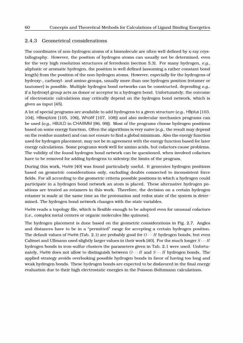
60 Concepts and Theoretical Methods for Calculations of Ligand Binding Energetics
2.4.3 Geometrical considerations
The coordinates of non-hydrogen atoms of a biomolecule are often well defined by x-ray crys-tallography. However, the position of hydrogen atoms can usually not be determined, evenfor the very high resolution structures of ferredoxin (section 5.3). For many hydrogen, e.g.,aliphatic or aromatic hydrogen, the position is well defined (assuming a rather constant bondlength) from the position of the non-hydrogen atoms. However, especially for the hydrogens ofhydroxy-, carboxyl- and amino-groups, usually more than one hydrogen position (rotamer ortautomer) is possible. Multiple hydrogen bond networks can be constructed, depending e.g.,if a hydroxyl group acts as donor or acceptor in a hydrogen bond. Unfortunately, the outcomeof electrostatic calculations may critically depend on the hydrogen bond network, which isgiven as input [45].
A lot of special programs are available to add hydrogens to a given structure (e.g., HBplus [103,104], HBexplore [105, 106], Whatif [107, 108]) and also molecular mechanics programs canbe used (e.g., HBUILD in CHARMM [96, 99]). Most of the programs choose hydrogen positionsbased on some energy function. Often the algorithms is very naive (e.g., the result may dependon the residue number) and can not ensure to find a global minimum. Also the energy functionused for hydrogen placement, may not be in agreement with the energy function based for laterenergy calculations. Some programs work well for amino acids, but cofactors cause problems.The validity of the found hydrogen bond network can be questioned, when involved cofactorshave to be removed for adding hydrogens to sidestep the limits of the program.
During this work, Hwire [40] was found particularly useful. It generates hydrogen positionsbased on geometric considerations only, excluding doubts connected to inconsistent forcefields. For all according to the geometric criteria possible positions in which a hydrogen couldparticipate in a hydrogen bond network an atom is placed. These alternative hydrogen po-sitions are treated as rotamers in this work. Therefore, the decision on a certain hydrogenrotamer is made at the same time as the protonation and redox state of the system is deter-mined. The hydrogen bond network changes with the state variables.
Hwire reads a topology file, which is flexible enough to be adopted even for unusual cofactors(i.e., complex metal centers or organic molecules like quinone).
The hydrogen placement is done based on the geometric considerations in Fig. 2.7. Anglesand distances have to be in a “permitted” range for accepting a certain hydrogen position.The default values of Hwire (Tab. 2.1) are probably good for O · · ·H hydrogen bonds, but evenCalimet and Ullmann used slightly larger values in their work [40]. For the much longer S · · ·Hhydrogen bonds in iron-sulfur clusters the parameters given in Tab. 2.1 were used. Unfortu-nately, Hwire does not allow to distinguish between O · · ·H and S · · ·H hydrogen bonds. Theapplied strategy avoids overlooking possible hydrogen bonds in favor of having too long andweak hydrogen bonds. These hydrogen bonds are expected to be disfavored in the final energyevaluation due to their high electrostatic energies in the Poisson-Boltzmann calculations.

2.4. Molecular Modeling 61
D
HA Xd1
d2
α
ε
LP
XALP
D Hζ
Figure 2.7. Hydrogen bond criteria of Hwire. Donor atom (D), acceptor atom (A), hydrogenatom (H) and lone pair (LP) geometries are described by two distances and three angles. Thedistance d1 is between the proton (H) and the acceptor (A), the distance d2 is between thedonor (D) and the acceptor (A). α is the angle between donor (D), hydrogen (H) and acceptor(A). ε is the angle between the hydrogen (H), the acceptor (A) and any of the acceptor lonepairs (LP), if they exist. The angle ζ is defined for hydrogen bonds involving a sp2 acceptoror donor. ζ is defined as angle of the hydrogen bond with respect to the plain LP, A, X (or X’,D, H for a donor).
Default value Value used
0 ≤ d1 ≤ 2.5 3.8
0 ≤ d2 ≤ 3.9 4.5
α ≥ 120.0 110.0
ε ≤ 45.0 180.0
ζ ≤ 45.0 180.0
Table 2.1. Hwire parameters given as default and used in this work. Distances d1 and d2
are given in A, angles α, ε and ζ are given in degree.

62 Concepts and Theoretical Methods for Calculations of Ligand Binding Energetics
2.5 Summary
In section 2.1, chemical reactions in terms of equilibrium constants and chemical potentialswere introduced. Microscopic and macroscopic binding constants were distinguished and itwas found that both microstates and macrostates can be described by microscopic energies.However, it was also shown that a macroscopic description is not sufficient to describe theenergetics of a system with more than one ligand binding site.
Section 2.1.2 introduced chemical potentials as a useful concept to describe chemical reac-tions. The common description of acid-base equilibria in terms of solution pH and dissociationconstant of the acid (pKa value, section 2.1.4) were introduced. It was shown, that an analo-gous description of redox equilibria in terms of reduction potential of the solution and stan-dard reduction potential of the redox active group (section 2.1.5) can be given. For moleculeswith a single proton or electron binding site the titration behavior can be described by thecommonly known Henderson-Hasselbalch and Nernst equations, respectively. For moleculeswith more binding sites a statistical mechanics description in terms of chemical potentialsand binding free energies will be introduced in section 3.1.
An important contribution to the energy function is the electrostatic energy term, which iscalculated using a continuum electrostatics approach. Therefore, the linearized Poisson-Boltzmann equation (LPBE) was derived from the first Maxwell equation (section 2.2) andit was outlined, how the LPBE can be solved numerically by finite difference methods (sec-tion 2.2.6). More details will be given in section 3.2.
Quantum chemistry (QM), especially Density Functional Theory (DFT), was introduced (sec-tion 2.3), because it is required for optimizing structures, calculating energies of formationand vibration of reactants and products and as basis for the fitting of charges. QM derivedenergy terms will be used as part of the energy function in particular in section 3.3. Theenergetics of small structural changes like rotamer energies may be described by QM, butthey can be calculated faster and not necessarily less accurate by molecular mechanics (MM,section 2.4.1 and section 3.4). Instead to obtain conformational energies describing largerstructural changes, either available experimental values or energies calculated by MM can beused, while QM calculations are usually too costly. Other classical mechanic models, i.e., thedescription of rotamers by a library (section 2.4.2) or the placement of hydrogens based ongeometric criteria (section 2.4.3), were briefly discussed, because they are used for structurepreparation (section 4.6) for subsequent ligand binding energy calculations.

CHAPTER 3
A GENERALIZED THEORY FOR CALCULATIONS
OF LIGAND BINDING ENERGETICS
In the previous chapter, a rigorous statistical mechanics description of ligand binding wasavoided, because the aim was to give only a flavor of the problems to be studied. Now, theligand binding will be described in the grand canonical ensemble (section 3.1.1) and it willbe shown how microscopic and macroscopic properties can be calculated from the grandcanonical partition function (section 3.1.3). In practice, the calculation of the grand canonicalpartition function is often not affordable and therefore an approximate treatment based onMonte Carlo calculations (section 3.1.4) is introduced. An energy function for the microstateenergy composed of contributions for each instances of each sites is given (section 3.1.2).Since this energy function is dominated by electrostatic energy contributions, the continuumelectrostatic model is described in more detail, i.e., it is formulated to become applicable formolecular calculations (section 3.2). Energy contributions are defined for a concise descrip-tion of energies of instances of sites (in section 3.3 and section 3.4).
I will refer to sites as sets of atoms described by different coordinates (rotamers) or directlyinvolved in binding of one or more ligands (of potentially different types). Electrostatic inter-actions between sites are described in the model, but not electronic interactions. For practicalreasons, sites should be as small as possible, but the partial charges of the atoms should addup to an integer charge and π-bonds should not be divided. Due to binding of ligands, thecharges and coordinates of sites change. The different combinations of charge forms and ro-tamer forms are called instances. Larger structural changes, which can not be well describedby rotamers, can be included as conformers. Usually, conformers are based on differentstructures obtained at potentially different chemical or physical conditions. A more detaileddiscussion can be found in section 3.2.2.
Two possible descriptions of sites will be introduced. One description is based on experimen-tally determined binding energies of model compounds in solution. The effect of transferringthe site from the model compound environment into the protein environment is calculated(section 3.4). The other description is based on quantum chemical calculations (section 3.3).It can be used, if no experimental data is available or if the site is too complex for an accurateexperimental description. Such experimental problems determining energies for model com-pounds can arise e.g., from strong electronic coupling between the ligands binding to the sitehindering a decomposition of the microstates (as it is the case for benzoquinone, section 5.5),
63

64 A Generalized Theory for Calculations of Ligand Binding Energetics
or from instability of the site outside of the protein hindering synthesis of model compounds(as it is the case for the iron-sulfur center of ferredoxin, section 5.3).
The physical description of the system is general in respect to the number of sites, the numberof instances per site, the number of ligands in the system and the number of ligands binding toeach single site. Sites described by model compounds or by quantum mechanical calculationscan be mixed. This physical model allows for titration calculations in a high-dimensionalchemical potential space. It is implemented in the program QMPB (section 4.3), which scaleslinearly with the number of instances and number of CPUs due to a suitable formulation ofthe energy function in this chapter.
At the end of this chapter, the energy function is compared with the functions used in pre-vious works. It is shown that the previous formulations only cover the special case of twoinstances per site (section 3.5). The limitations of the previous model are underlined, e.g.,leading to serious approximations for including rotamers. The previous treatment of sitesby quantum chemistry was hampered by the lack of appropriate programs resulting in anexponential growth of computational cost with the number of instances and the inability tocombine the quantum chemical treatment with the model compound based treatment of sites(i.e., calculation of interaction energies with acceptable computational cost).
3.1 Towards an Energy Function for Ligand Binding
Section 2.1 introduced chemical reactions in terms of equilibrium constants and chemicalpotentials. Microscopic and macroscopic equilibrium constants can be calculated from mi-crostate energies. The connection between the microstate and the macrostate is formed by thethe grand canonical partition function (section 3.1.1). A suitable microstate energy functionis described in section 3.1.2. How to calculate probabilities and equilibrium constants fromthe grand canonical partition function is discussed in section 3.1.3.
3.1.1 The Grand Canonical Partition Function
To describe ligand binding energetics the grand canonical ensemble was chosen, which allowsligand molecules to enter and leave the system during simulation. The macroscopic state ofthe system is defined by a set of thermodynamic variables {µλ}:
{µλ} ={T , V , µ1, . . . , µλ, . . . , µNligand
}, (3.1)
where T is the absolute temperature, V the volume and µλ the chemical potential of ligandtype λ (λ = 1 . . . Nligand). The temperature T is a simple variable in the calculations. Moderatechanges of the temperature do not affect the calculations significantly, since the temperatureenters the calculation inverse in the thermodynamic β (β = 1
RT ) or the inverse Debye lengthκ(~r) (eq. 2.68). A larger effect is the dependence of the electrical permittivity ε(~r) on the tem-perature, i.e., the dielectric constants have to be adopted accordingly. The volume V has notto be further defined, since the electrostatic model usually considers a single macromolecularcomplex (molecule) in an infinite implicit solvent. This model describes well a highly dilute

3.1. Towards an Energy Function for Ligand Binding 65
solute. Since the chemical potentials µλ (section 2.1.2) of all ligand types λ are the mostimportant in the set of thermodynamic variables, the symbol {µλ} was chosen.
The grand canonical partition function Ξ is the sum of the partition functions of all conforma-tions i, Ξi, for a given set of thermodynamic variables {µλ}:
Ξ({µλ}) =Nconf∑i
Ξi({µλ}) (3.2)
The grand canonical partition function Ξi of conformation i is a Boltzmann weighted sum ofNmicro,i energies of the ensemble of microstates Gmicro(~xi,n, {µλ}) (characterized by their statevector ~xi,n and a set of thermodynamic variables {µλ}):
Ξi({µλ}) =Nmicro,i∑
n
σ(~xi,n, {µλ}) exp(−βGmicro(~xi,n, {µλ})
)(3.3)
Here, σ(~xi,n, {µλ}) is the symmetry number (degeneracy factor).
There are Nmicro,i =∏Nsite,ij Ninstance,i,j microstates, where Nsite,i is the number of sites in con-
former i and Ninstance,i,j is the number of instances in site j of conformer i (Ninstance,i,j is gen-erally any natural number, but in the titration theory with a binary state vector, section 3.5,it is two).
The symmetry number σ(~xi,n, {µλ}) for the microstate with energy Gmicro(~xi,n, {µλ}) is equal toone as long as all microstates are represented explicitly, what is assumed in the following.For achiral molecules, there might be several isoenergetic microstates, which can be trans-ferred into each other by symmetry operations. In this cases, the symmetry number has to betaken into account. Proteins have many chirality centers and therefore impose a chiral envi-ronment onto ligand molecules. In calculations of ligand molecules in solution (e.g., quinonein solution, section 5.5) the symmetry number might be important [109]. Also a symmet-ric ligand might have multiple isoenergetic microstates in the unbound form, which becomenon-isoenergetic upon binding to the protein (section 3.3).
Each microstate n of conformation i is characterized by an individual state vector ~xi,n
~xi,n =(x1i,n, . . . , x
ji,n, . . . , x
li,n, . . . , x
Nsite,ii,n
)(3.4)
Instances k ≡ xji,n and m ≡ xli,n are the values of the state vector ~xi,n at the position j and l,respectively. I will refer to instance k and m of site j and l as jk and lm, respectively.
3.1.2 The Microstate Energy Function
The microstate energy Gmicro(~xi,n, {µλ}) was introduced in section 2.1.3 as sum of the standardenergy of the microstate G◦(~xi,n) and the stoichiometric factor νλ times the chemical potentialµλ summed over the Nligand ligand types λ (eq. 2.21). It was pointed out, that the stoichiometricfactor is relative to a freely chosen reference state. Here, I set the reference state as the(hypothetic) fully unbound state, i.e., that Nλ(~xi,n) is the number of bound ligands of type λ to

66 A Generalized Theory for Calculations of Ligand Binding Energetics
the molecule. The conformational energy Gconf,i is the energy of conformer i.
Gmicro(~xi,n, {µλ}) = Gconf,i +G◦(~xi,n)−Nligand∑λ
Nλ(~xi,n)µλ (3.5)
For practical calculations it is not feasible to calculate all possible microstates separately, i.e.,the standard energy of each microstate G◦(~xi,n). I assume, that the standard energy can besplit into a sum of contributions of each instance k of site j, the intrinsic energy Gintr,i(jk), anda contributions due to the interaction with each instance m of each other site l, the interactionenergy Ginter,i(jk, lm):
G◦(~xi,n) =Nsite,i∑j
Gintr,i(jk) +12
Nsite,i∑j
Nsite,i∑l 6=j
Ginter,i(jk, lm). (3.6)
This assumption of additivity is true, if a MM force field or electrostatic energies calculated bythe Poisson equation or LPBE (section 3.2) are used. The number of bound ligands Nλ(~xi,n) =∑Nsite,ij nλ,i(jk) can also be split into contributions of each site, so that nλ,i(jk) is the number
of ligands of type λ bound to instance jk. Therefore, the microstate energy can be written as
Gmicro(~xi,n, {µλ}) = Gconf,i+Nsite,i∑j
(Gintr,i(jk)−
Nligand∑λ
nλ,i(jk)µλ
)+
12
Nsite,i∑j
Nsite,i∑l 6=j
Ginter,i(jk, lm). (3.7)
By exploiting the assumed additivity as in eq. 3.7, the computational cost reduces from
O
(∑Nconfi
∏Nsite,ij Ninstance,i,j
)(for eq. 3.5) to O
(∑Nconfi
∑Nsite,ij Ninstance,i,j
)(for eq. 3.7). For
example, a system with two conformers and 11 sites with 10 instances each, has 2 · 1011
microstates, but the formulation in eq. 3.7 reduces the computational cost to calculating2 · 11 · 10 = 220 intrinsic energies, which is assumed to be the time determining step (i.e., solv-ing the LPBE). The double sum of the interaction energy does not contribute significantly tothe computational cost, since it is a simple multiplication, as will be shown in section 3.2.7.Both, the matrix of Gintr,i(jk) values and the tensor of Ginter,i(jk, lm) values can be stored andlooked up upon calculating the microstate energy Gmicro(~xi,n, {µλ}) in a separate step.
Each conformation i has a user defined conformational energy Gconf,i. The conformationalenergy can be calculated by a MM force field (section 2.4) or it can be used to weight differentexperimental structures according to experimental results. When calculating the conforma-tional energy, it is important to exclude all energy contributions, which enter the calculation ofthe microstate energy by other terms, i.e., electrostatic interactions between sites or rotamerenergies.
The intrinsic energy Gintr,i(jk) describes the energy of instance k of site j in a different envi-ronment (e.g., the environment of a model compound or in vacuum) and the energy for trans-ferring the instance of the site from the different environment into the protein environment(section 3.2.5). It contains the energy due to interaction of instance jk with the background(charge) set of atoms, i.e., all atoms not belonging to any site. The intrinsic energy Gintr,i(jk)is defined differently for sites which are parameterized based on QM calculations (section 3.3)or based on experimental results (section 3.4).

3.1. Towards an Energy Function for Ligand Binding 67
The interaction energy Ginter,i(jk, lm) describes the interaction of the current instance k of sitej with instance m ≡ xli,n of any other site l according to the state vector ~xi,n of microstate n.The factor 1
2 is to correct for double counting the interaction of instance jk with instance lm
and instance lm with instance jk, because the double sum runs twice over all Nsite,i sites.
It would be possible to use microstate energies Gmicro(~xi,n, {µλ}) as in eq. 3.3 directly. However,numerical errors might result, if the exponential of the energy approaches the precision ofthe number representation in a computer. Therefore, it is useful to define a reference stateGmicro(ref, {µλ}) such, that Gmicro(~xi,n, {µλ}) has small values (i.e., for the most contributingspecies in the statistical average, eq. 3.10):
∆Gmicro(~xi,n, {µλ}) = Gmicro(~xi,n, {µλ})−Gmicro(ref, {µλ}) (3.8)
This shift of the zero point of the microstate energies does not change the relative populationof the microstates to each other. It only reduces the numerical error significantly.
3.1.3 Calculation of Properties Based on the Partition Function
Microstate n in conformer i has for a given set of thermodynamic variables {µλ} a population(or probability) of
〈~xi,n({µλ})〉 =σ(~xi,n, {µλ})
Ξi({µλ})exp(−βGmicro(~xi,n, {µλ})
)(3.9)
The symmetry number σ(~xi,n, {µλ}) was discussed in section 3.1.1. The probability 〈x(jk, {µλ})〉of site j being in instance k can be calculated using a delta function δi,n(jk), which is one, ifxji,n = k and zero otherwise:
〈x(jk, {µλ})〉 =Nconf∑i
Nmicro,i∑n
δi,n(jk)〈~xi,n({µλ})〉 (3.10)
or for a particular conformation i
〈xi(jk, {µλ})〉 =Nmicro,i∑
n
δi,n(jk)〈~xi,n({µλ})〉 (3.11)
By changing the chemical potential µλ of ligand type λ (in the set of thermodynamic variables{µλ}), the population of instance k of site j varies, leading to probability curves (or titrationcurves) for this instance.
The uptake of ligand λ is the total average number 〈Xλ〉 of ligands of type λ bound to themolecule. It is given by the sum of the probabilities of each microstate 〈~xi,n〉 multiplied by thetotal number of ligands of type λ Nλ(~xi,n), bound in the particular microstate:
〈Xλ〉 =Nconf∑i
Nmicro,i∑n
Nλ(~xi,n)〈~xi,n〉 (3.12)
In general, as stated in section 2.1.1, microscopic and macroscopic equilibrium constants canbe determined from microscopic free energies. The microscopic equilibrium constant for the

68 A Generalized Theory for Calculations of Ligand Binding Energetics
reaction, where microstate n = 1 is the reactant state and microstate n = 2 is the productstate, is given by:
K~xi,2
~xi,1= exp
(−β(G◦(~xi,2)−G◦(~xi,1))
)(3.13)
The Nλth macroscopic equilibrium constant of ligand type λ is given by:
KNλ =
∑Nconfi
∑Nmicro,in δ
(Nλ(~xi,n)− 1
)exp(−β(Gconf,i +G◦(~xi,n))
)∑Nconfi
∑Nmicro,in δ
(Nλ(~xi,n)
)exp(−β(Gconf,i +G◦(~xi,n))
) (3.14)
The delta function δ(Nλ(~xi,n)) is defined to be one, if the microstate with state vector ~xi,n hasNλ bound ligands of the type λ and zero otherwise.
3.1.4 Approximating Probabilities of Microstates
Most of the equations in section 3.1.3 depend on the knowledge of all Nmicro,i microstateenergies in each of the Nconf conformers to calculate the partition function Ξ:
Nconf ·Nmicro,i =Nconf∑i
Nsite,i∏j
Ninstance,i,j (3.15)
An example in section 3.1.2 showed, that this number is very large already for moderatesystems. Except for very small systems, the partition function can not be calculated explicitly(by programs as SMT, implemented by Matthias Ullmann). A number of schemes exist [27,36, 110–113] to approximate the probability 〈~xi,n({µλ})〉 of a microstate without evaluatingthe partition function. In this work, the Metropolis Monte Carlo (MMC) method is used.The Adaptive Mesh Refinement (AMR, section 4.2.3) method can focus the MMC calculationson regions in chemical potential space, which are of interest since the probabilities are notconstant. AMR can also reduce the number of instances, which need to be sampled, andfinally the state vector length by removing instances, which are known not to be populated ina certain part of chemical potential space.
A property of the Boltzmann distribution in the grand canonical partition function is, thatmicrostates with low energy contribute exponentially more than microstates with high energy.Therefore, a sampling method, which finds an ensemble of low energy microstates, is able toobtain a good approximation of the probability of microstates significantly contributing in thegrand canonical partition function. A Monte Carlo (MC) method with importance sampling (asimplemented by Matthias Ullmann in the program GMCT) is suitable for this purpose.
For a given set of thermodynamic variables {µλ} and for a random conformation i an initialstate vector ~xi,n is generated randomly. In a MC move, the instance m of a randomly-chosensite j is changed to a randomly-chosen instance k. The energy change between instance m

3.1. Towards an Energy Function for Ligand Binding 69
State Vector
Random Inital
Conformation and
Equilibrate
as Arithmetic Average
over Saved State Vectors
Calculate Probabily
Accept new
Instance k
Save
State Vector
yes
no
yes
Calculate
new oldG (x) − G (x)
Choose new
Conformer
Accept new
Conformer
Return to old
Conformer
Conformer
Different
i
Metropolisyes
no yes
MC moves
More
MC scans
More
no
yes
no no
Choose new
Site j
Choose new
Instance k
Calculate
G (j ,j )∆ i km
Return to old
Instance m
Metropolis
Figure 3.1. Flowchart of the Metropolis Monte Carlo procedure to approximate the proba-bility of microstates. The probability of all instances is calculated from a pre-defined numberof low energy microstates instead of calculating the statistical average from the ensemble ofall possible microstates (eq. 3.10). The procedure is described in the text. The equilibrationstep is equivalent to the loop over the number of MC scans, except that the protonationstate vectors are not saved.
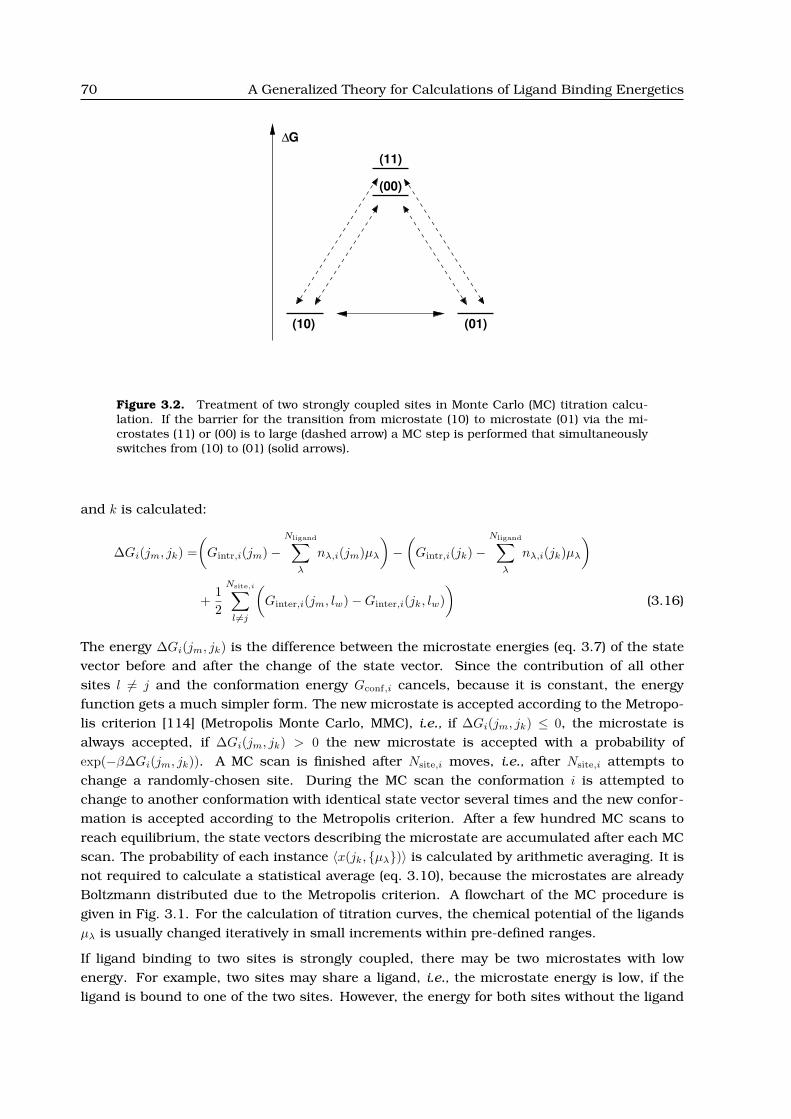
70 A Generalized Theory for Calculations of Ligand Binding Energetics
(00)
(11)
(10) (01)
∆G
Figure 3.2. Treatment of two strongly coupled sites in Monte Carlo (MC) titration calcu-lation. If the barrier for the transition from microstate (10) to microstate (01) via the mi-crostates (11) or (00) is to large (dashed arrow) a MC step is performed that simultaneouslyswitches from (10) to (01) (solid arrows).
and k is calculated:
∆Gi(jm, jk) =(Gintr,i(jm)−
Nligand∑λ
nλ,i(jm)µλ
)−(Gintr,i(jk)−
Nligand∑λ
nλ,i(jk)µλ
)
+12
Nsite,i∑l 6=j
(Ginter,i(jm, lw)−Ginter,i(jk, lw)
)(3.16)
The energy ∆Gi(jm, jk) is the difference between the microstate energies (eq. 3.7) of the statevector before and after the change of the state vector. Since the contribution of all othersites l 6= j and the conformation energy Gconf,i cancels, because it is constant, the energyfunction gets a much simpler form. The new microstate is accepted according to the Metropo-lis criterion [114] (Metropolis Monte Carlo, MMC), i.e., if ∆Gi(jm, jk) ≤ 0, the microstate isalways accepted, if ∆Gi(jm, jk) > 0 the new microstate is accepted with a probability ofexp(−β∆Gi(jm, jk)). A MC scan is finished after Nsite,i moves, i.e., after Nsite,i attempts tochange a randomly-chosen site. During the MC scan the conformation i is attempted tochange to another conformation with identical state vector several times and the new confor-mation is accepted according to the Metropolis criterion. After a few hundred MC scans toreach equilibrium, the state vectors describing the microstate are accumulated after each MCscan. The probability of each instance 〈x(jk, {µλ})〉 is calculated by arithmetic averaging. It isnot required to calculate a statistical average (eq. 3.10), because the microstates are alreadyBoltzmann distributed due to the Metropolis criterion. A flowchart of the MC procedure isgiven in Fig. 3.1. For the calculation of titration curves, the chemical potential of the ligandsµλ is usually changed iteratively in small increments within pre-defined ranges.
If ligand binding to two sites is strongly coupled, there may be two microstates with lowenergy. For example, two sites may share a ligand, i.e., the microstate energy is low, if theligand is bound to one of the two sites. However, the energy for both sites without the ligand

3.2. Continuum Electrostatics at Atomic Detail 71
bound or both with a ligand bound may be significantly higher. The energy difference may belarge enough to make the transfer of the ligand from one site to the other unlikely, if one ofthe intermediate states has to be passed through (Fig. 3.2). The problem can be avoided bychanging the instance of both sites simultaneously - a so-called double-move. The move isalso accepted according to the Metropolis criterion. In analogy, triple-moves are possible forthe case that three sites couple strongly.
3.2 Continuum Electrostatics at Atomic Detail
In section 2.2 continuum electrostatics was introduced by deriving the Poisson, Poisson-Boltzmann (PBE) and linearized Poisson-Bolzmann (LPBE) equation from Gauss’s law. It wasalso discussed, how the PBE and LPBE can be solved numerically. The treatment was usuallybased on the general concept of a charge distribution ρ(~r), but in the context of the Coulombequation (section 2.2.2) also point charges q were introduced.
This section concentrates on the atomic description within the continuum electrostatic model,focussed to be useful for the calculation of contributions to the microstate energy function(section 3.1.2). It is explained, why additivity of electrostatic potentials is required (sec-tion 3.2.1), how boundaries are defined for rotamers and conformers and what the conse-quences of the two descriptions of molecular flexibility are (section 3.2.2). The conceptsof Born and background energies are introduced (section 3.2.3 and section 3.2.4) and it isshown how they can be used to calculate transfer energies from homogeneous and heteroge-neous environments into the protein (section 3.2.5 and section 3.2.6). Finally, the electrostaticinteraction energy, as it is used in eq. 3.7, is introduced (section 3.2.7).
3.2.1 Point Charges
For practical calculations on molecular systems, usually a point charge qa is associated withthe coordinate of each atom a:
ρ(~r) =Natom∑
a
qa(~ra) (3.17)
The values of point charges are often taken from MM force fields (section 2.4.1) and have non-integer values (partial charges) to describe correctly dipoles and higher multipoles. However,sets of atoms - so-called charge groups - have an integer charge. Since systems with non-integer charge are usually physically not meaningful, care has to be taken when dividing thesystem into smaller sub-systems (i.e., sites) ensuring that each fraction always has an integercharge (i.e., each instance). Integer charges can be assured, when always only completecharge groups (or several charge groups at once) are transferred from one sub-system toanother. If charges are calculated quantum chemically (section 2.3), attention has to be payedfor including only complete charge groups into the calculation. Else the quantum chemicallyderived charges are not compatible to the force field charge group approach.
Electrostatic energies (as charge times electrostatic potential, eq. 2.57) are additive when theelectrostatic potential ϕ(~ra) is calculated by the Poisson equation or LPBE. The non-linearizedPBE, however, is not additive due to the exponential term of the Boltzmann distribution,

72 A Generalized Theory for Calculations of Ligand Binding Energetics
but this additivity is retrieved by linearization in the LPBE. The calculation of the microstateenergy, eq. 3.7, contains electrostatic energy terms for each instance of each site, thus it is ofcrucial importance to evaluate the potentials ensuring additivity. Due to this additivity, thecomputational cost for calculating the electrostatic energy contributions is drastically reduced(section 3.1.2). Hence, the computational cost using the PBE is prohibitive for ligand bindingstudies on usual proteins or a probably small error is made assuming the same additivity forthe PBE.
3.2.2 Dielectric Boundaries
In section 2.2.6, it was pointed out that the result of electrostatic calculations depend criticallyon the dielectric boundaries. The method to calculate solvent accessible surfaces based onatom coordinates and radii was described. For the interior of the surfaces a different dielectricconstant is assigned compared to the solvent.
In section 3.1.2, I introduced conformers and assigned them a conformer energy, Gconf,i. Adifferent conformation has a significantly different protein structure. Therefore, it must havedifferent dielectric boundaries in the continuum electrostatics calculations. All instances ofall sites have to be calculated separately for each set of dielectric boundaries, thus the compu-tational cost multiplies by the number of conformations. Instead, a common set of dielectricboundaries is defined by the coordinates of all atoms of the protein in all their instances (i.e.,all rotamer forms and with all ligands bound) so that an additional (rotamer) instance addsonly a single calculation of the LPBE. However, rotamers are a coarser approximation due tothe common set of dielectric boundaries. Therefore, the choice between conformers and ro-tamers is sometimes a trade-off. For small ligands, small changes between the rotamers (i.e.,hydrogen rotamers) and buried sites with the same dielectric constant as the backgroundset, the approximation by the common set of dielectric boundaries is good. In other cases itdepends on the system.
3.2.3 Born Energy
The Coulomb energy eq. 2.58 became infinity if the distance between the central point of thecharge distribution and the point of the potential measurement became zero in a homoge-neous dielectric. In case of the Poisson equation (eq. 2.59) the dielectric media is generallynot homogeneous, but the electrical permittivity ε depends on the point in space ~r. The dielec-tric boundaries ~∇ε(~r) shield the electrostatic field (eq. 2.52), so that the electrostatic energyρϕ(~r; ρ) is finite. The electrostatic field ϕ(~r; ρ) acting back on the charge distribution ρ is calledreaction field. The electrostatic energy due to the interaction of a charge distribution ρ withits reaction field is called Born energy. Usually for molecular systems, the charge distributionρ is described by (partial) point charges qa at positions ~ra of atoms a: The Born energy istherefore written as:
GBorn =12
Natom∑a
qaϕ(~ra; ρ) (3.18)

3.2. Continuum Electrostatics at Atomic Detail 73
The electrostatic potential ϕ(~ra; ρ) at the center of an atom a, depends on one hand on theposition ~ra of the atom, on the other hand on the charge distribution ρ of this and all otheratoms (given by their partial charge and position).
The factor 12 originates from the linear response approximation: The Born energy is related to
the work charging a cavity from qi = 0 to qf within a uncharged macroscopic dielectric body.The reaction field acting back at the inducing charge is assumed to be proportional to q andof opposite sign:
ρ = Cq; C < 0 (3.19)
The work of charging from qi = 0 to qf is then
Welec =∫ qf
0
ρdq
=∫ qf
0
Cqdq
=C
2qf
2
=12ϕfqf < 0,
(3.20)
where ϕf is the reaction field potential (or back potential) at the end of the charging process.The effective charging work does not equal the charge times the potential, but only half of it.The missing work is the energy cost of polarizing the polarizable media [115].
3.2.4 Background Energy
Additionally to the charge distribution ρ of the atom set of interest, there might be fixedcharges Qa in the system leading to the so-called background energy:
Gback =Natom∑
a
Qaϕ(~ra; ρ) (3.21)
The electrostatic potential ϕ(~ra; ρ) at the point of a background charge Qa, depends on onehand on the position ~ra of the background charge, on the other hand on the charge distribu-tion ρ of all atoms of the atom set of interest.
An electrostatic energy is generally the sum of Born and background energy:
Welec = GBorn +Gback (3.22)
A very important property of the background energy is that it is symmetric: With ρq being thecharge distribution of charges qa at the positions ~ra and ρQ being the charge distribution ofcharges Qb at the positions ~rb the following is valid:
Natom∑a
qaϕ(~ra, ρQ) =Natom∑b
Qbϕ(~rb; ρq) (3.23)

74 A Generalized Theory for Calculations of Ligand Binding Energetics
∆G (j )homotrans,i k
ε = 4
ε = 80
jk
w
pε = 4
jk
p
Figure 3.3. Calculation of a homogeneous transfer energy ∆Ghomotrans,i(jk). εp is thedielectric constant of the protein and εw is the dielectric constant of the solvent, e.g., water.
This property is independent of the background energy being calculated from the Poisson,Poisson-Boltzmann or the linearized Poisson-Boltzmann equation.
The linear response approximation relates the Born energy to the work of charging a cavity(section 3.2.3). However, for isolated systems (i.e., the thermodynamic cycles described below)the charge has to remain constant (conservation of charge). Instead, the difference in elec-trostatic energy due to transferring the charge of instance k of site j in conformer i from onepoint in space to another is the objective of the calculations. In this work, the destination of allcharge transfers is the heterogeneous protein system, which consists of at least two dielectricregions (the protein and the aqueous solvent), but two types of transfer energies can be distin-guished, dependent on the source of the charge transfer: The source can be a homogeneousenvironment with same dielectric constant as the site or a heterogeneous environment, wherethe site is part of a model compound embedded in a different dielectric region (e.g., aqueoussolvent).
3.2.5 Homogeneous Transfer Energy
The source of the charge transfer is a homogeneous dielectric environment (Fig. 3.3). Theheterogeneous transfer energy is the sum of Born and background energy for transferringinstance jk of conformer i:
∆Ghomotrans,i(jk) = ∆GBorn,homotrans,i(jk) +Gback,homotrans,i(jk) (3.24)
The difference in Born energy is calculated as:
∆GBorn,homotrans,i(jk) = GBorn,protein,i(jk)−GBorn,homo,i(jk)
=12
Natom,i,jk∑a
qa,i(jk)ϕprotein(~ra,i; ρi(jk))− 12
Natom,i,jk∑a
qa,i(jk)ϕhomo(~ra,i; ρi(jk))
=12
Natom,i,jk∑a
qa,i(jk)[ϕprotein(~ra,i; ρi(jk))− ϕhomo(~ra,i; ρi(jk))]
(3.25)

3.2. Continuum Electrostatics at Atomic Detail 75
∆ solv,i kG (j )
ε = 1
jk
v
jk
ε = 1v
ε = 80w
Figure 3.4. Calculation of a solvation energy ∆Gsolv,i(jk). εv is the dielectric constant ofvacuum and εw is the dielectric constant of the solvent, e.g., water.
There are Natom,i,jk partial charges qa,i(jk) of instance k of site j, which interact with the elec-trostatic potential ϕprotein(~ra,i; ρi(jk)) in the protein environment and with the electrostatic po-tential ϕhomo(~ra,i; ρi(jk)) in the homogeneous dielectric. The electrostatic potentials are due to
the charge distribution ρi(jk) =Natom,i,jk∑
aqa,i(jk).
In the calculations described here, there are no background charges present in the homoge-neous dielectric, but only in the protein environment. Therefore, the background energy ofinstance k of site j in conformer i is:
Gback,homotrans,i(jk) = Gback,protein,i(jk)
=Nback,i∑a
Qprotein,a,iϕprotein(~ra,i; ρi(jk))(3.26)
The background (charge) set of the protein has Nback,i charges Qprotein,a,i, which interact withthe electrostatic potential ϕprotein(~ra,i; ρi(jk)) of instance jk, identical to the potential calcu-lated for the Born energy. The background charge set is constant for all sites of a particularconformer i. Therefore, calculating the background energy only requires additional multipli-cations.
For the special case, where the homogeneous dielectric is vacuum, the electrostatic energy iscalled solvation energy (Fig. 3.4):
∆Gsolv,i(jk) = ∆GBorn,homotrans,i(jk) +Gback,homotrans,i(jk) (3.27)
The solvation energy is the difference in energy of a molecule in vacuum and in a given solvent(described by a dielectric constant εr). Born calculated the solvation energy of spherical ions ina homogeneous solvent analytically [116]. Therefore the energy difference due to the differencein the electric field in different media is called Born solvation energy.
In fact, the solvation energy discussed here is only the electrostatic part. A full solvationenergy would include the work for creating a cavity for the atoms in the solute. This workis largely entropy dependent and can only be estimated from the surface area and someempirical factor [117, 118]. In the titration calculations only the difference in solvation energybetween charge forms is calculated. The boundaries are kept constant so that the cavity doesnot change and therefore there is no associated work to be done.

76 A Generalized Theory for Calculations of Ligand Binding Energetics
G (j )∆ heterotrans,i kε = 80w
pε = 4
jk
ε = 4
ε = 80
j
w
p
k
Figure 3.5. Calculation of a heterogeneous transfer energy. εp is the dielectric constant ofthe protein and εw is the dielectric constant of the solvent, e.g., water.
3.2.6 Heterogeneous Transfer Energy
The source of the charge transfer is a heterogeneous dielectric environment (Fig. 3.5). Usuallya model compound in solution is used as reference point. The transfer of a subset of charges(those belonging to instance k of site j) of the model compound into the protein environmentis calculated. The coordinates (rotamer form) remain the same. The heterogeneous transferenergy is the sum of Born and background energy:
∆Gheterotrans,i(jk) = ∆GBorn,heterotrans,i(jk) + ∆Gback,heterotrans,i(jk) (3.28)
The difference in Born energy is calculated as:
∆GBorn,heterotrans,i(jk) = GBorn,protein,i(jk)−GBorn,model,i(jk)
=12
Natom,i,jk∑a
qa,i(jk)ϕprotein(~ra,i; ρi(jk))− 12
Natom,i,jk∑a
qa,i(jk)ϕmodel(~ra,i; ρi(jk))
=12
Natom,i,jk∑a
qa,i(jk)[ϕprotein(~ra,i; ρi(jk))− ϕmodel(~ra,i; ρi(jk))]
(3.29)
There are Natom,i,jk partial charges qa,i(jk) of instance k of site j, which interact with the elec-trostatic potential ϕprotein(~ra,i; ρi(jk)) in the protein environment and with the electrostatic po-tential ϕmodel(~ra,i; ρi(jk)) in the heterogeneous dielectric environment of the model compound.
The electrostatic potential is due to the charge distribution ρi(jk) =Natom,i,jk∑
aqa,i(jk) of the atoms
a in instance k of site j in conformer i.
Usually there are background charges present in the model compound, i.e., charges which arenot transferred into the protein environment. The protein has a different set of backgroundcharges, which are identical to those discussed for the homogeneous transfer energy. The
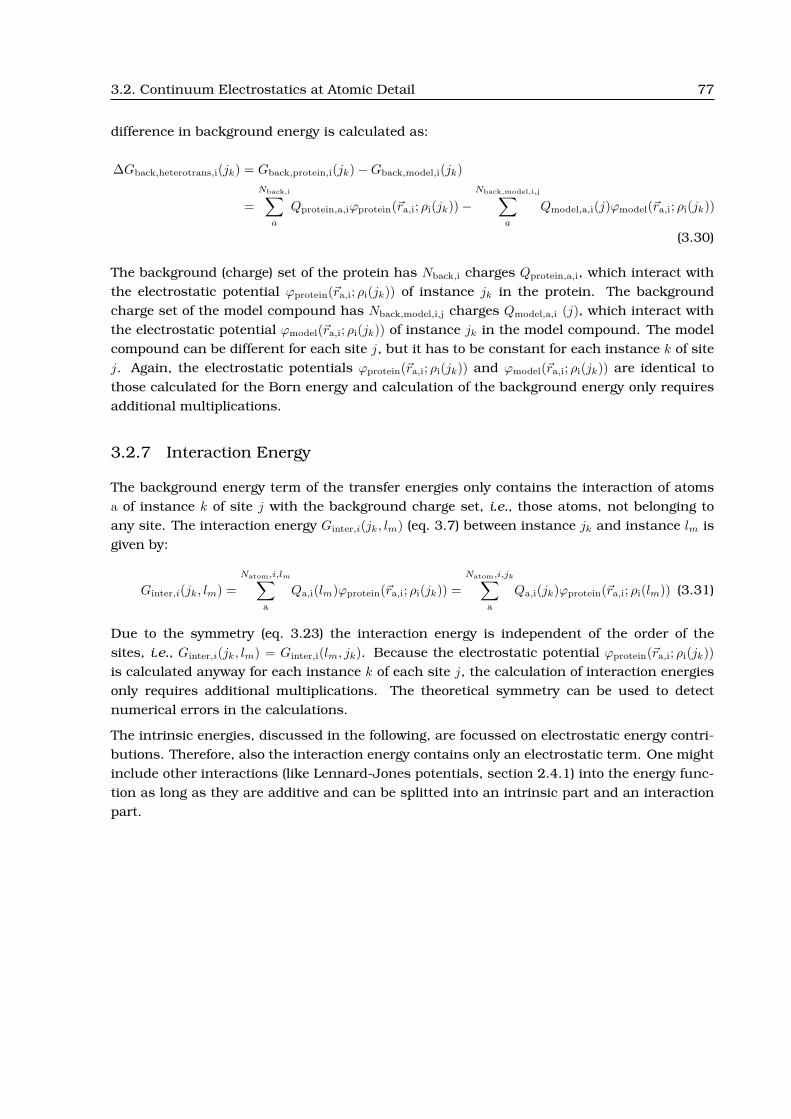
3.2. Continuum Electrostatics at Atomic Detail 77
difference in background energy is calculated as:
∆Gback,heterotrans,i(jk) = Gback,protein,i(jk)−Gback,model,i(jk)
=Nback,i∑a
Qprotein,a,iϕprotein(~ra,i; ρi(jk))−Nback,model,i,j∑
a
Qmodel,a,i(j)ϕmodel(~ra,i; ρi(jk))
(3.30)
The background (charge) set of the protein has Nback,i charges Qprotein,a,i, which interact withthe electrostatic potential ϕprotein(~ra,i; ρi(jk)) of instance jk in the protein. The backgroundcharge set of the model compound has Nback,model,i,j charges Qmodel,a,i (j), which interact withthe electrostatic potential ϕmodel(~ra,i; ρi(jk)) of instance jk in the model compound. The modelcompound can be different for each site j, but it has to be constant for each instance k of sitej. Again, the electrostatic potentials ϕprotein(~ra,i; ρi(jk)) and ϕmodel(~ra,i; ρi(jk)) are identical tothose calculated for the Born energy and calculation of the background energy only requiresadditional multiplications.
3.2.7 Interaction Energy
The background energy term of the transfer energies only contains the interaction of atomsa of instance k of site j with the background charge set, i.e., those atoms, not belonging toany site. The interaction energy Ginter,i(jk, lm) (eq. 3.7) between instance jk and instance lm isgiven by:
Ginter,i(jk, lm) =Natom,i,lm∑
a
Qa,i(lm)ϕprotein(~ra,i; ρi(jk)) =Natom,i,jk∑
a
Qa,i(jk)ϕprotein(~ra,i; ρi(lm)) (3.31)
Due to the symmetry (eq. 3.23) the interaction energy is independent of the order of thesites, i.e., Ginter,i(jk, lm) = Ginter,i(lm, jk). Because the electrostatic potential ϕprotein(~ra,i; ρi(jk))is calculated anyway for each instance k of each site j, the calculation of interaction energiesonly requires additional multiplications. The theoretical symmetry can be used to detectnumerical errors in the calculations.
The intrinsic energies, discussed in the following, are focussed on electrostatic energy contri-butions. Therefore, also the interaction energy contains only an electrostatic term. One mightinclude other interactions (like Lennard-Jones potentials, section 2.4.1) into the energy func-tion as long as they are additive and can be splitted into an intrinsic part and an interactionpart.

78 A Generalized Theory for Calculations of Ligand Binding Energetics
∆GQM,i
∆G intr,i
∆ ∆G (j )solv,i kG (j )solv,i m
ε = 1
ε = 80 ε = 80
ε = 1
ε = 4 ε = 4
j
j
j
j
w
p
v v
w
v
p
m
m
k
k
v
ε = 1
ε = 1
Figure 3.6. Intrinsic energy calculation based on QM calculations. The energy differencebetween two instances k and m of a quantum center j in vacuum ∆GQM,i = (Hvac,i(jk) +Gvib,i(jk) + Gfree,i(jk)) − (Hvac,i(jm) + Gvib,i(jm) + Gfree,i(jm)) can be calculated by QM (sec-tion 2.3). The solvation energies ∆Gsolv,i(jm) = ∆GBorn,homotrans,i(jm) + Gback,homotrans,i(jm) −Gcorr,i(jm) and ∆Gsolv,i(jk) = ∆GBorn,homotrans,i(jk) + Gback,homotrans,i(jk) − Gcorr,i(jk) can becomputed by continuum electrostatics (section 3.2.5). The energy difference between thetwo instances in the protein is the difference of their intrinsic energy ∆Gintr,i = Gintr,i(jk) −Gintr,i(jm) (eq. 3.32).
3.3 Intrinsic Energies based on Quantum Chemical Data
The method of calculating so-called absolute1 intrinsic energies, described here, allows toobtain microstate energies of sites for which no specific experimental values are available.Instead quantum mechanical (QM) calculations are used to parameterize the site. The proce-dure follows the thermodynamic cycle in Fig. 3.6.
Often it is difficult to synthesize model compounds with the same geometry as in the protein.Especially metal clusters are often instable, when they are extracted from the protein envi-ronment. The organic scaffold synthesized to stabilize the cluster and adjust its geometry isoften so complex and non-protein like (very aromatic and hydrophobic) that it is questionablehow well it is suited as model compound. Experiments with these model compounds are oftenmade in complex organic solvents and not in water, which may lead to additional complica-tions for the transferability of the results. In other cases as heme proteins, the puckering ofthe porphyrin or the out-of-plane position of the iron due to the fifth and sixth ligand mayplay an important role, which is hard to reproduce in synthetic model compounds. Further,a site may bind several ligands and there is a strong electronic coupling between the lig-and binding sites. An example is quinone (section 5.5), which binds two electrons and twoprotons. Despite remarkable experimental attempts to characterize this biological important
1Absolute is used here in contrast to the relative intrinsic energy, where the shift in energy of an instance iscalculated relative to the energy of the instance in a model compound in solution. Certainly, the underlying quantummechanical calculations are not based on first principles, but the basis sets (section 2.3.1) and exchange correlationfunctions (section 2.3.1) are tuned to obtain chemically reasonable results. Furthermore, each standard reductionpotential is (by definition) relative to the potential of the standard hydrogen electrode and each pKa value is relativeto the solvation energy of the proton. Both (closely related) values have to be measured and calculations are relativeto these values.

3.3. Intrinsic Energies based on Quantum Chemical Data 79
system, there is still no complete picture. In other cases, the sites are only stable for a shorttime (as phosphoserine and phosphohistidine, section 5.2) or have many tautomers (e.g., nu-cleic acids), that it is impossible to obtain pure microstates in experiment. As discussed insection 2.1, there are also sever limitations on the number of microstate energies which areexperimentally obtainable from microscopic equilibrium constants.
For the method described here, only the (experimental) standard chemical potential of eachligand type in solution is needed, i.e., the standard chemical potential of electrons and protonsto characterize all proton and electron binding sites. Each instance of the site is parameter-ized by quantum chemical and continuum electrostatic calculations. The clear benefit is theindependence of specific experimental data, but the disadvantage is that errors in the QMmethods or the charge fitting enter the calculations, often leading to less accurate resultsas relative calculations, when appropriate experimental data is available. Rotameric or tau-tomeric instances of sites can be parameterized in exactly the same way.
The absolute intrinsic energy Gintr,i(jk) (in eq. 3.7) for an instance k of site j in conformer i isthe sum of a homogeneous transfer energy (section 3.2.5) and energy terms, which can mostlybe calculated by QM (section 2.3), i.e., Born energy ∆GBorn,homotrans,i(jk)(eq. 3.25) and background energy Gback,homotrans,i(jk) (eq. 3.26), the QM energy of formationHvac,i(jk), the vibrational energy Gvib,i(jk), an energy correction Gcorr,i(jk) and an energy ofunbound ligand molecules Gfree,i(jk):
Gintr,i(jk) = ∆GBorn,homotrans,i(jk)+Gback,homotrans,i(jk)+Hvac,i(jk)+Gvib,i(jk)−Gcorr,i(jk)+Gfree,i(jk)
(3.32)
The energy of formation (total bonding energy) Hvac,i(jk) is the energy of the site and all boundligands given by the QM program after geometry optimization. The vibrational energy Gvib,i(jk)can be obtained by QM frequency calculations.
3.3.1 Energy Correction
If the quantum region is covalently bound to the protein, there are electrostatic interactionsin the Poisson-Boltzmann energies between bonded atoms or those sharing a bond angle.These interactions would be excluded in normal force field calculations (section 2.4.1) becausethey depend on the electronic structure, i.e., orbital geometries and can not be describedproperly by the Coulomb equation. Instead force fields include extra bonded and angle terms,which coarsely model these interactions. In case of relative ligand binding energy calculations,model compounds are defined, which include bonded atoms and those sharing a bond angle.Therefore, these critical electrostatic energies are canceled by subtracting the backgroundenergy of the site in the model compound and in the protein. For absolute ligand bindingenergy calculations this interaction energy can be calculated and the results corrected by
Gcorr,i(jk) =Natom∑a
Nbond a,angle a,i∑A
Qprotein,A,iϕprotein(~ra,i; qa,i(jk)), (3.33)
where A are those Nbond a,angle a,i atoms (with charge Qprotein,A,i) of the background set, whichare in bond or in angle relationship with atom a of the quantum region (Fig. 3.7). The cor-

80 A Generalized Theory for Calculations of Ligand Binding Energetics
Q1 M1
M2
M2
M2
Q2
Q2
Q2
QM MM
Figure 3.7. Correction for interactions between the quantum region (QM) and the regiondescribed by force field charges (MM). The atoms marked Q1 and M1 are covalently bound inthe protein, but belong to the QM and MM region, respectively. The atoms Q2 are covalentlybound to Q1 and the atoms M2 are covalently bound to M1. The electrostatic interactionbetween the bonded atoms Q1 and M1 (red), as well as the electrostatic interactions betweenthe atoms having a bond angle, i.e., Q2 −M1 (green) and M2 −Q1 (blue), would be excludedin a force field. The additional electrostatic interactions in the intrinsic energy Gintr,i(jk) canbe canceled by a correction term Gcorr,i(jk), which is calculated by additional electrostaticcalculations only containing the appropriate atoms.
rection energy can also be given as input to avoid repetitive calculation or to include alsoother energy terms like the Lennard-Jones term, which is assumed to be constant betweeninstances.
3.3.2 Energy of Free Ligands
The bulk solvent in the calculations is a mixture of water, ions and ligands. The modelcombines calculations of transfer energies in an implicit continuum model with explicit ligandmolecules considered upon ligand binding. If the intrinsic energy of each instance Gintr,i(jk)(eq. 3.32) contains also the energy of formation and vibrational terms of the ligands boundto the instance (Hvac,i(jk) and Gvib,i(jk), respectively) as well as electrostatic energy terms(∆GBorn,homotrans,i(jk), Gback,homotrans,i(jk) and Gcorr,i(jk)), than the electrostatic energy terms,the energy of formation, as well as vibrational, translational and entropic terms of the freeligands need to be considered, too. The energy of unbound ligand molecules, Gfree,i(jk) ineq. 3.32, accounts for those energy terms:
Gfree,i(jk) =Nligand∑λ
νλ,i(jk)µ◦λ =Nligand∑λ
(νλ,i(j)− nλ,i(jk)
)µ◦λ (3.34)

3.3. Intrinsic Energies based on Quantum Chemical Data 81
The stoichiometric factor νλ,i(jk), i.e., the number of explicit unbound ligands, can be definedby the number of ligands bound to a particular instance jk, nλ,i(jk), and a reference numberof ligands νλ,i(j). The number of bound ligands is identical with nλ,i(jk) in eq. 3.7.
The reference number of ligands νλ,i(j) can be freely chosen shifting the reference point inenergy, however only a few choices have a physical meaning associated. νλ,i(j) may be themaximal number of ligands λ site j can bind, so that nλ,i(jk) = νλ,i(j) in the fully bound form.An alternative useful definition could be that νλ,i(j) equals the maximum number of ligandsλ, which can bind to the protein at the same time or that νλ,i(j) equals the total number ofligands λ in the simulation. The advantage of the first definition is, that the number of bindingsites of the molecule for a certain ligand λ is not required for having a pool of ligands largeenough to fill all binding sites. Also the total number of ligands of type λ in the system isproblematic, because it depends on the chemical potential µλ of ligand type λ in the bulk. Bythe first definition only the number of ligands nλ,i(jk) of type λ bound to a certain instance jkis necessary. To parameterize the instance jk with nλ,i(jk) ligands bound by QM calculations,the composition of ligands and their orientation is required anyway. This definition makes theinput for instances of sites easier transferable between different systems.
The standard chemical potential µ◦λ of a single unbound ligand (νλ = 1) of type λ is given asinput µ◦λ = G◦λ − RT lnσ(λ). Here, σ(λ) is the symmetry factor of ligand λ in bulk solution (seediscussion in section 3.1.1). For electrons, protons and spherical ions σ(λ) = 1. For othermolecules σ(λ) may have different values, i.e., σ(H2O) = 2, σ(H3O
+) = 3, σ(HPO2−4 ) = 12 etc..
The last example takes the four oxygens the proton can be bound to into account as well asthe three isoenergetic rotamers the proton can have in each of the four bound forms.
The standard chemical potential µ◦λ has to be calculated in analogy to the site (eq. 3.32).In particular, the terms Hvac and Gvib have to be calculated by the same QM method. Thesolvation energy may be calculated by continuum electrostatic methods or experimentallyobtained. The background energy term, correction energy term and interaction energy termare usually zero for a ligand.
The standard chemical potential µ◦H+ of a single free proton can be calculated as:
µ◦H+ = Hvac(H+) + ∆GBorn(H+) +Gtrans(H+) + ∆(PV )− T [S(H+)] (3.35)
Hvac(H+) is the energy of formation of the proton. Dependent on the definition of the zero-point in energy of the QM program it might be zero (Gaussian) or not (ADF). The Born solvationenergy of the proton ∆GBorn(H+) = −260.5kcal
mol can be calculated from the experimentally mea-sured potential of the standard hydrogen electrode [119]. The translational energy of a protonGtrans(H+) = 3
2kBT and the energy change due to the volume change in the gas phase reac-tion ∆(PV ) = kBT are estimated from the ideal gas approximation. The entropic portion ofthe gas-phase free energy of the proton T [S(H+)] = 7.8kcal
mol is derived from the Sackur-Tetrodeequation.
The standard chemical potential µ◦e− of a single free electron can be calculated from the ex-perimental potential of the standard hydrogen electrode ∆SHE ≈ −4.43V [120]:
µ◦e− = F∆SHE (3.36)

82 A Generalized Theory for Calculations of Ligand Binding Energetics
∆G intr,i
∆Gmodel
∆G (j )heterotrans,i k∆G (j )heterotrans,i m
mj
mj kj
kjε = 80
ε = 4
ε = 80w
ε = 4
ε = 80
ε = 4
ε = 80
ε = 4p
w w
p
p
w
p
Figure 3.8. Intrinsic energy calculation relative to a model compound (without ro-tamers). The energy difference ∆Gmodel between two charge forms jm and jk of a modelcompound is known in solution. The heterogeneous transfer energies ∆Gheterotrans,i(jk) and∆Gheterotrans,i(jm) can be computed by continuum electrostatics (section 3.2.6). The energydifference between the two charge forms in the protein is the difference of their intrinsicenergy Gintr,i(jk) (eq. 3.37).
3.4 Intrinsic Energies based on Experimental and
Molecular Mechanics Data
Using the thermodynamic cycle shown in Fig. 3.8, relative intrinsic energy calculations al-low to obtain microstate energies for experimentally well characterized sites. Model com-pounds have been synthesized, which are geometrically and chemically similar to the site inthe protein environment. Equilibrium constants have been measured, which allow to calcu-late microstate energies of the model compound in solution. For example, the sidechain andbackbone pKa values of all amino acids are measured in tripeptides and dipeptides, respec-tively. These results can be used to calculate the pKa shift for the amino acids in the proteinenvironment by electrostatic methods. Such calculations generally show good agreement withmeasurements of apparent pKa values in the protein. Also for other ligands such calculationscan be done. Unlike the absolute intrinsic energy calculations, relative intrinsic energy cal-culations do not depend on computationally expensive quantum mechanical calculations anderrors in the charge model seem to cancel out quite well.
Relative intrinsic energies can be calculated for sites with more than one rotamer form bymolecular (or quantum) mechanics. Rotamers allow to include sidechain flexibility and differ-ent hydrogen bond networks (due to rotation of hydroxyl groups) into continuum electrostaticcalculations. Sites may bind ligands and have multiple rotamer forms.
The relative intrinsic energy Gintr,i(jk) for an instance k of site j is the sum of a transfer energy(section 3.2.5 or section 3.2.6), the energy of a model compound in the same instance (charge

3.4. Intrinsic Energies based on Experimental and Molecular Mechanics Data 83
and rotamer form) ∆Gmodel(jk) and the internal energy of the rotamer form ∆Grotamer(jk):
Gintr,i(jk) = ∆GBorn,i(jk) + ∆Gback,i(jk) + ∆Gmodel(jk) + ∆Grotamer(jk) (3.37)
The model energy ∆Gmodel(jk) is the ligand binding energy of the model compound relative to areference charge form. For a site binding a single proton, the model energy of the protonatedform is ∆Gmodel(protonated) = −RT ln 10pKa,model and the model energy of the deprotonatedform is ∆Gmodel(deprotonated) = 0 (or ∆Gmodel(protonated) = 0 and ∆Gmodel(deprotonated) =RT ln 10pKa,model, respectively). The energy of formation, vibrational and entropic terms aswell as the energy associated with the unbound ligand are all hidden in the experimentalmodel energy.
The differences in Born energy ∆GBorn,i(jk) and background energy ∆Gback,i(jk) are the dif-ference in electrostatic energy of the site in the model compound environment and in theprotein environment. For sites having different charge forms heterogeneous transfer energies(section 3.2.6) and for sites having different rotamer forms homogeneous transfer energies(section 3.2.5) are calculated, respectively. For sites having both, different charge and ro-tamer forms, both transfer energies are computed.
In theory, each rotamer form would have a slightly different model energy. Usually, therotamer form is not determined together with the model energy, but the model energy ismeasured for an ensemble of rotamers in solution. Therefore, it is probably the best approx-imation to attribute the model energy to the rotamer with the lowest internal energy (whichis therefore the most populated in the experimental ensemble) and calculate the intrinsic en-ergies of all instances relative to this rotamer form. This reference rotamer has a rotamerenergy ∆Grotamer(jk) = 0 and all non-reference rotamers have a rotamer energy relative to thereference rotamer.
3.4.1 Non-Ligand Binding Reference Rotamer Form
Site j has several rotamer forms, but only one charge form, and instance k is chosen to be thereference rotamer form. Therefore, the intrinsic energy is set to zero
Gintr,i(jk) = 0 (3.38)
and the energy of all other rotamers is given relative to this instance.
In Fig. 3.9, instance jk = q1r1 would be a reference rotamer form without model compound, ifonly the red thermodynamic cycle would be calculated.
3.4.2 Ligand Binding Reference Rotamer Form
Site j has several charge forms and one or more rotamer forms. The rotamer form of instancek is chosen to be the reference rotamer for the site j. There has to be one reference instanceper charge form, but all reference instances have to belong to the same rotamer form. Theintrinsic energy
Gintr,i(jk) = ∆GBorn,heterotrans,i(jk) + ∆Gback,heterotrans,i(jk) + ∆Gmodel(jk) (3.39)

84 A Generalized Theory for Calculations of Ligand Binding Energetics
∆Gmodel
∆Grotamer
∆Gheterotrans,i ∆Gheterotrans,i
intr,i 1 2G (q r )∆
intr,i 2 1G (q r )∆
ligand bindingenergy
rotamerenergy
ε = 80w
ε = 80w
pε = 4
pε = 4pε = 4
pε = 4
ε = 80w
pε = 4
ε = 80w ε = 80w
pε = 4 pε = 4
∆Ghomotrans,i
∆Ghomotrans,i
qq2r1
q1
r1
r1q r12
1
q1r2
q1r1
q1r2
G (q r )intr,i 1 1
Figure 3.9. Thermodynamic cycles for relative energy calculations. The red cycle de-scribes the calculation of rotamer energies, the yellow cycle describes the calculation ofligand binding energies. The site j with chargeset q1 and coordinate set r1 is the refer-ence instance for both charges and rotamers (thick frame). The intrinsic energy of theinstance is Gintr,i(jref) = Gintr,i(q1r1) = 0, if all other instances differ only in the coor-dinate set (e.g., q1r2, section 3.4.1). If also other chargeforms exist (e.g., q2r1), the in-trinsic energy of the instance is Gintr,i(jref) = Gintr,i(q1r1) = ∆Gheterotrans,i(q1r1). If theinstance is in the reference rotamer form, but not the reference chargeform, the intrin-sic energy is Gintr,i(q2r1) = ∆Gheterotrans,i(q2r1) + ∆Gmodel (section 3.4.2). If the instanceis not the reference rotamer, but no other chargeforms exist, the intrinsic energy isGintr,i(q1r2) = ∆Ghomotrans,i(q1r2) − ∆Ghomotrans,i(q1r1) + ∆Grotamer(jk) (section 3.4.3). If theinstance is not the reference rotamer and other chargeforms exist, the intrinsic energy isGintr,i(q1r2) = ∆Ghomotrans,i(q1r2)−∆Ghomotrans,i(q1r1)+∆Grotamer(jk)+∆Gheterotrans,i(q1r1). Theequation can be simplified following the dashed arrow (section 3.4.4).

3.4. Intrinsic Energies based on Experimental and Molecular Mechanics Data 85
contains a heterogeneous transfer energy (section 3.2.6) and a model energy ∆Gmodel(jk),which is zero for the reference charge form. The rotamer energy ∆Grotamer(jk) is always zeroin a reference rotamer form.
In Fig. 3.9, instance jk = q1r1 would be a reference rotamer form with model compound, if theyellow (and maybe the red) thermodynamic cycle would be calculated.
3.4.3 Non-Ligand Binding Non-Reference Rotamer Form
Site j has several rotamer forms, but only one charge form, and instance k is not chosen tobe the reference rotamer form.
A homogeneous transfer energy (section 3.2.5) of instance jk relative to the reference rotamerjref is calculated. The model energy ∆Gmodel(jk) is zero. The rotamer energy ∆Grotamer(jk) is thedifference in internal energy of instance k relative to the reference rotameric form. Therefore,the intrinsic energy is given by
Gintr,i(jk) =∆GBorn,homotrans,i(jk)−∆GBorn,homotrans,i(jref) +Gback,homotrans,i(jk) (3.40)
−Gback,homotrans,i(jref) +Grotamer(jk)−Grotamer(jref).
In Fig. 3.9, instance jk = q1r2 would be a non-reference rotamer form without model com-pound, if only the red thermodynamic cycle would be calculated. The difference in homoge-neous transfer energy between instance q1r2 and jref = q1r1 needs to be calculated.
3.4.4 Ligand Binding Non-Reference Rotamer Form
Site j has several rotamer forms and several charge forms. Instance k is not chosen to be thereference rotamer form.
The difference in homogeneous transfer energy (section 3.2.5) of instance jk relative to thereference rotamer jref plus the heterogeneous transfer energy (section 3.2.6) of instance jref
has to be calculated:
∆GBorn,i(jk) = GBorn,protein,i(jk)−GBorn,homo,i(jk) +GBorn,homo,i(jref)−GBorn,model,i(jref)(3.41)
∆Gback,i(jk) = Gback,protein,i(jk)−Gback,model,i(jref) (3.42)
The energies GBorn,protein,i(jref) and Gback,protein,i(jref) would occur for the homogeneous trans-fer energy with a negative sign and for the heterogeneous transfer with a positive sign andtherefore cancel out. The model energy ∆Gmodel(jref) is specified for the the model compoundin the reference rotameric form. The rotamer energy ∆Grotamer(jk) is the difference in internalenergy of instance k relative to the reference rotameric form. Hence, the intrinsic energy canbe written as
Gintr,i(jk) = ∆GBorn,i(jk) + ∆Gback,i(jk) + ∆Gmodel(jref) +Grotamer(jk)−Grotamer(jref). (3.43)

86 A Generalized Theory for Calculations of Ligand Binding Energetics
In Fig. 3.9, instance jk = q1r2 would be a non-reference rotamer form with model compound,if both the red and the yellow thermodynamic cycle would be calculated. The difference inhomogeneous transfer energy between instance q1r2 and jref = q1r1 and the heterogeneoustransfer energy of instance q1r1 needs to be calculated.
3.5 Comparison to Previously Used Energy Functions
3.5.1 Calculations based on Experimental Data
In this work, a state vector ~xi,n (eq. 3.4) was introduced, which allows a varying numberof instances k ≡ xji,n for each site j. Many binding events, however, can be described by twoforms, a bound form and an unbound form only. Previous works used a binary state vector, sothat k = 0 in the unbound form and k = 1 in the bound form. For a protein with Nsite,i bindingsites and two forms each, the total number of microstates is Nmicro,i = 2Nsite,i . The contributionof a site to the microstate energy was described as an energy difference between bound andunbound form instead of energies associated with each individual instance. Instead of thegeneral description by chemical potentials and energies, specific formulations were used aspH and pKa or E and E◦ [121, 122]. In fact, the program used before (Multiflex), is only thoughtto be used for pKa calculations. Standard reduction potential calculations have to be done inpKa-units. The user has to keep track of the different ligand types and recalculate energiesfor subsequent titration calculations. Therefore, only pKa calculations will be discussed here.
Multiflex allows only relative pKa calculations (relative to a model compound, section 3.4) ina two dielectric environment (protein and solvent). Instead of the intrinsic energy Gintr,i(jk)(eq. 3.37) an intrinsic pKa value is calculated:
pKa,intr,i(j) = pKa,model(j)−1
RT ln 10
(∆∆GBorn,i(j) + ∆∆Gback,i(j)
)(3.44)
The pKa value describes the deprotonation equilibrium of an acid (section 2.1.4) at site j.The double differences in Born and background energy, describes first the difference betweenthe model compound environment and the protein environment in the heterogeneous transfer(section 3.2.6) and second the difference between the protonated j� and deprotonated j♦
charge form.
∆∆GBorn,i(j) = ∆GBorn,heterotrans,i(j�)−∆GBorn,heterotrans,i(j♦) (3.45)
∆∆Gback,i(j) = ∆Gback,heterotrans,i(j�)−∆Gback,heterotrans,i(j♦) (3.46)
The model pKa value, pKa,model(j), is the experimental pKa value of a model compound of sitej in aqueous solution. The intrinsic pKa value, pKa,intr,i(j) is here directly the pKa value ofsite j if all other sites are in their reference state.
Microstate energies are calculated relative to a reference state, which is chosen to be theneutral protonation form. The protein is not divided into a background charge set and theinteraction energy of instances of sites, but the background energy includes all interactionsof site j with all other sites in their reference charge form.

3.5. Comparison to Previously Used Energy Functions 87
O O
O
O
O
O
O
−
O
H+ H
H
H
Figure 3.10. A carboxylic acid has different tautomers and rotamers in the protonatedform.
The interaction energy ∆∆Ginter,i(j, l) between sites j and l can be written as double differenceof interaction energies Ginter,i(jk, lm) (eq. 3.31):
∆∆Ginter,i(j, l) =(Ginter,i(j�, l�)−Ginter,i(j♦, l�)
)−(Ginter,i(j�, l♦)−Ginter,i(j♦, l♦)
)(3.47)
The microstate energy can be written (using equations from section 2.1.4) as:
Gmicro(~xi,n,pH) = Gconf,i +Nsite,i∑j
[xji,n − xji,ref ]
[RT ln 10
(pH− pKa,intr,i(j)
)]
+12
Nsite,i∑j
Nsite,i∑l 6=j
[xji,n − xji,ref ][x
li,n − xli,ref ]∆∆Ginter,i(j, l)
(3.48)
As in eq. 3.7, Gconf,i is the conformational energy. The first sum runs over all sites to calculatethe difference of intrinsic pKa value (intrinsic energy) and pH (chemical potential of protons inthe bulk solvent) and the second sum adds the interaction energy with all other sites. Sitesonly contribute to the microstate energy, if they are in a different protonation form than inthe reference state and interaction energy is only added if both sites are not in their referenceform. The sign of the contribution is positive if the site in the reference form (xji,ref and xli,ref ,respectively) is deprotonated and the site in the form of interest is deprotonated, which isthe case for bases. Acids have a protonated reference form and the contribution is negative.In the generalized formulation this complexity arising from the filter function ([xji,n − xji,ref ]and [xli,n − xli,ref ], respectively) is avoided, because the energies are not calculated relative toa physical reference state. Instead an artificial state is chosen as reference state, where allatoms belonging to instances of sites are uncharged.
Treatment of Carboxyl-, Amine-, Hydroxyl- and Thiol-Groups
In the last two decades, the approach described above was successfully used for many appli-cations [13, 35–44], even though the calculation of pKa values with a single protonated form isstrictly only valid for sites with no tautomers or rotamers. Since no amino acid strictly fulfillsthis requirement for proton binding (Fig. 3.10 and Fig. 3.11), a single average charge distri-bution (set of partial charges) describes the bound form and another the unbound form of thesite. The carboxyl-group of acidic amino acid sidechains (i.e., aspartate and glutamate) and

88 A Generalized Theory for Calculations of Ligand Binding Energetics
N
N
N
N
N
N
+
H
H
H
H+
+
H
H
−tautomer
−tautomerδ
ε
Figure 3.11. Histidine has two tautomers in the singly protonated form (protonated on Nδ1or Nε2 with pKa values of 7.0 and 6.6 in solution, respectively). The doubly protonated formis shown as well. The doubly deprotonated form has a pKa value of about 14.0 in solutionand can therefore be excluded for most calculations.
the C-terminus can be described by a single protonated form, where the proton has a positionbetween the two oxygens (as the first tautomer in Fig. 3.10). The average charge distributionavoids the problem of the two tautomers and the rotameric forms, where the protonated acidis a hydrogen bond donor. Also the basic amino acids, i.e., lysine and the N-terminus canbe described by a amine-group with or without positive charge and arginine can be describedby a charged or uncharged guanidinium group. For hydroxyl- and thiol-groups (of cystein,tyrosine, serine and threonine), however, this method is problematic, since the calculated pKa
values of neighboring titrateable groups depends strongly on the presence of hydrogen bonds.The orientation of the hydrogen atom has to be assigned before the pKa calculations introduc-ing a bias if different hydrogen bond networks are possible [45]. Certainly, different hydrogenbonds would also affect, the pKa value of the hydroxyl- and thiol-groups, but usually thesegroups were not considered as titrateable due to their high pKa value. However, to studyproton-transfer (section 5.6) this approximation is not sustainable.
Treatment of Histidine
The amino acid, for which the shortcomings of the approach using a binary state vector be-comes most obvious is histidine (Fig. 3.11). The imidazole ring of histidine has two tautomersin the singly protonated form, which have the proton located on one or the other side ofthe imidazole ring. Therefore, the hydrogen bonding pattern is clearly different and also thetautomers have different pKa values. The doubly deprotonated form has a pKa value, whichis too high to be populated under physiological conditions. The solution of Bashford and

3.5. Comparison to Previously Used Energy Functions 89
coworkers [123] treats the tautomers as conformers, i.e., performing a continuum electro-static calculations of the complete protein for the δ- and ε-tautomer separately. Once theprotonation of the δ-tautomer at Nε2 is permitted to yield the doubly protonated form andonce the protonation and of the ε-tautomer at Nδ1 is permitted to yield the doubly protonatedform. Postprocessing of the calculated energies (by an additional program) is done to obtain abinary state vector with two bits for histidine. The fully deprotonated form, which was nevercalculated, but exists in the state vector, was assigned an arbitrary high energy to avoid pop-ulation in the titration calculations. All interaction energies with histidine have to be modifiedto be correct for the modified physical model. For N histidines 2 + N Multiflex calculations(titrating all residues) are necessary. The results are correct in the physiological pH range,but the methodology is computational expensive for many histidines and non-intuitive. It isnot transferable with acceptable effort to other sites like quinones (section 5.5).
Treatment of Rotamers
The insufficiency of the approach doing calculations with a binary state vector became evenmore evident, when You and Bashford included rotamer forms into the pKa value calcula-tions [51]. Effectively, the You and Bashford treatment of rotamers, calculates a thermody-namic average pKa,intr,i for a site, when all other sites are in their reference form. It wouldbe correct to include the rotamer forms equivalently to the charge forms as independent mi-crostates. This would allow to adopt the rotamer population to the charge forms of surround-ing sites. However, such a treatment is not possible with a binary state vector and requires amore general physical model, as it is described in this work.
For inclusion of rotamers into pKa calculations, eq. 3.44 is extended by You and Bashford [51](β = 1
RT ):
pKa,intr,i(j) = pKa,model(j)−1
RT ln 10lnNrotamer,i,j∑
r
[exp(−β∆Genv,i(j♦
r,protein))
− exp(−β∆Genv,i(j�
r,protein))
− exp(−β∆Genv,i(j♦
r,model))
+ exp(−β∆Genv,i(j�
r,model))]
(3.49)
The protonated j� and unprotonated j♦ form of site j in rotamer r are calculated in the proteinenvironment jprotein and model environment jmodel. The free energy ∆Genv,i is given as thesum of Born ∆GBorn,i, background ∆Gback,i and a non-electrostatic, charge form independentenergy ∆Grotamer:
∆Genv,i = ∆GBorn,i + ∆Gback,i + ∆Grotamer (3.50)

90 A Generalized Theory for Calculations of Ligand Binding Energetics
The Born and background energies are calculated as homogeneous transfer energies (sec-tion 3.2.5):
∆GBorn,i(j♦r,protein) = ∆GBorn,homotrans,i(j♦
r,protein) = GBorn,protein,i(j♦r )−GBorn,homo,i(j♦
r )
∆GBorn,i(j�r,protein) = ∆GBorn,homotrans,i(j�
r,protein) = GBorn,protein,i(j�r )−GBorn,homo,i(j�
r )
∆GBorn,i(j♦r,model) = ∆GBorn,homotrans,i(j♦
r,model) = GBorn,model,i(j♦r )−GBorn,homo,i(j♦
r )
∆GBorn,i(j�r,model) = ∆GBorn,homotrans,i(j�
r,model) = GBorn,model,i(j�r )−GBorn,homo,i(j�
r )
∆Gback,i(j♦r,protein) = Gback,homotrans,i(j♦
r,protein) = Gback,protein,i(j♦r )
∆Gback,i(j�r,protein) = Gback,homotrans,i(j�
r,protein) = Gback,protein,i(j�r )
∆Gback,i(j♦r,model) = Gback,homotrans,i(j♦
r,model) = Gback,model,i(j♦r )
∆Gback,i(j�r,model) = Gback,homotrans,i(j�
r,model) = Gback,model,i(j�r )
The Born energy needs the additional subtraction of the potential of the site in a homogeneousdielectric ϕhomo(~ra,i; ρi(jr)) with dielectric constant of the interior of the site. This term isneeded to remove grid artefacts, which were canceled in the single-rotamer calculation by thedifference of protein and model compound energy.
Additionally to the terms in eq. 3.50, one might need to consider an additional term ∆Gselfback,i,which is the homogeneous transfer energy of the background charges of the protein
ρi,j,r,protein =Ni,j,r,protein∑
a
Qa,i(jr,protein) (3.51)
or model compound
ρi,j,r,model =Ni,j,r,model∑
a
Qa,i(jr,model), (3.52)
which changes due to the changing boundary with rotamer r of site j. If the boundary changessignificantly, one might even need to include the surface area dependent non-electrostatic partof the solvation energy.
∆Gselfback,i is computed as:
∆Gselfback,i(j♦r,protein) = ∆Gselfback,i(j�
r,protein) (3.53)
=12
Ni,j,r,protein∑a
Qa,i(jr,protein)[ ϕprotein(~ra,i; ρi,j,r,protein)
−ϕhomo(~ra,i; ρi,j,r,protein)]

3.5. Comparison to Previously Used Energy Functions 91
∆Gselfback,i(j♦r,model) = ∆Gselfback,i(j�
r,model) (3.54)
=12
Ni,j,r,model∑a
Qa,i(jr,model)[ ϕmodel(~ra,i; ρi,j,r,model)
−ϕhomo(~ra,i; ρi,j,r,model)]
The electrostatic potentials have to be calculated on a grid, which has to be larger than theprotein, but should be as fine as the grid of the finest focussing step of the site. Practicalcalculations on such a grid are not feasible due to memory requirements and computationalcost. For small changes of the dielectric boundary, this term is small, that I excluded it frommy calculation scheme assuming a combined dielectric boundary. In fact, in many cases, thegroups are buried and the dielectric boundary is unchanged. In cases, where the change issignificant, conformers can be used.
Despite the problematic inclusion of the rotamer energy into the intrinsic pKa value, thecalculation scheme including a molecular mechanics energy ∆Grotamer and a thermodynamiccycle using homogeneous transfers is very similar to the approach I describe in this work.However, my distinction between reference and non-reference rotamers avoids computationof GBorn,model,i(jr) and Gback,model,i(jr) for each non-reference rotamer in each charge form. Forcalculations with many rotamer forms and charge forms per site this optimization can lead toa significant saving in processor time.
Other Works to Include Protein Flexibility into Electrostatic Calculations
While methods for calculating protonation probabilities in proteins by continuum electrostaticmethods exist in a number of groups (Honig, Gunner, McCammon, Bashford, Wade, Vriend,Knapp, Ullmann and other), there are relatively few attempts to include protein flexibility.
Nielsen et al. [46] developed a method to calculate pKa values combining Whatif [107], DelPhi[28] and the package of Yang et al. [27]. Hydrogen atoms were placed and optimized bydifferent protocols and His, Asn and Gln were allowed to “flip”, i.e., rotate by 180◦ aroundthe χ2, χ2 and χ3 torsion angle, respectively. A threshold-accepting algorithm combined withtree search methods to optimize the global hydrogen bond network [108] was found to bethe preferable hydrogen placement method. The hydrogen placement problem was treated asprecursory step independent of the outcome of the pKa calculations. In another work [47]the authors used two structures (for strongly interacting groups four structures) per sitewith globally optimized hydrogen bond networks to compute Born and background energies.Therefore, the hydrogen bond network was always optimal to stabilize a certain protonationstate, however the energy to convert the system from a hydrogen bond network optimal forone protonation state to a hydrogen bond network optimal for another protonation state wasnot included into the microstate energy.
Maybe the most advanced method, multiconformational continuum electrostatics (MCCE),was developed in the group of Marilyn Gunner [32, 33]. Their energy function does not onlyinclude electrostatic terms, i.e., Born, background and interaction energy, but also a non-electrostatic contribution to the intrinsic energy and interaction energy and an entropy cor-rection. Their method allows to include hydrogen rotamers and tautomers. Singly-protonatedhistidine is described by two tautomers with the same model pKa value [32]. The method was
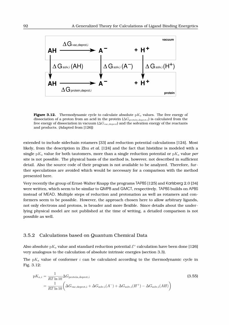
92 A Generalized Theory for Calculations of Ligand Binding Energetics
A− + H+
A− + H+
G∆ protein,deprot,i
G vac,deprot,i∆
(AH)G∆ solv,i G∆ solv,i (A ) − G∆ solv,i (H ) +
AH
vacuum
AH
protein
Figure 3.12. Thermodynamic cycle to calculate absolute pKa values. The free energy ofdissociation of a proton from an acid in the protein (∆Gprotein,deprot,i) is calculated from thefree energy of dissociation in vacuum (∆Gvac,deprot) and the solvation energy of the reactantsand products. (Adapted from [126])
extended to include sidechain rotamers [33] and reduction potential calculations [124]. Mostlikely, from the description in Zhu et al. [124] and the fact that histidine is modeled with asingle pKa value for both tautomers, more than a single reduction potential or pKa value persite is not possible. The physical basis of the method is, however, not described in sufficientdetail. Also the source code of their program is not available to be analyzed. Therefore, fur-ther speculations are avoided which would be necessary for a comparison with the methodpresented here.
Very recently the group of Ernst-Walter Knapp the programs TAPBS [125] and Karlsberg 2.0 [34]were written, which seem to be similar to QMPB and GMCT, respectively. TAPBS builds on APBSinstead of MEAD. Multiple steps of reduction and protonation as well as rotamers and con-formers seem to be possible. However, the approach chosen here to allow arbitrary ligands,not only electrons and protons, is broader and more flexible. Since details about the under-lying physical model are not published at the time of writing, a detailed comparison is notpossible as well.
3.5.2 Calculations based on Quantum Chemical Data
Also absolute pKa value and standard reduction potential E◦ calculation have been done [126]very analogous to the calculation of absolute intrinsic energies (section 3.3).
The pKa value of conformer i can be calculated according to the thermodynamic cycle inFig. 3.12:
pKa,i =1
RT ln 10∆Gprotein,deprot,i (3.55)
=1
RT ln 10
(∆Gvac,deprot,i + ∆Gsolv,i(A−) + ∆Gsolv,i(H+)−∆Gsolv,i(AH)
)

3.5. Comparison to Previously Used Energy Functions 93
The solvation energies (section 3.2.5) ∆Gsolv,i(A−) and ∆Gsolv,i(AH) can be calculated by con-tinuum electrostatics methods (e.g., with Solvate or Solinprot). The solvation energy of a proton∆Gsolv,i(H+) (identical with ∆GBorn(H+) = −260.5kcal
mol in eq. 3.35) can be calculated from theexperimentally measured potential of the standard hydrogen electrode. The gas phase depro-tonation energy ∆Gvac,deprot,i is calculated from:
∆Gvac,deprot,i = ∆Hvac,deprot,i + ∆Gvib,deprot,i +Gtrans(H+) + ∆(PV )− T [S(H+)] (3.56)
∆Hvac,deprot,i = Hvac,i(A−) + Hvac,i(H+) − Hvac,i(AH) is the difference in energy of formation invacuum of the dissociated (deprotonated and hydrogen ion) and associated (protonated) sys-tem. ∆Gvib,deprot,i is the change in vibrational energy between the protonated and deprotonatedform. Both terms can be calculated as by QM methods (section 2.3). The translational energyof a proton Gtrans(H+), the energy change due to the volume change in the gas phase reaction∆(PV ) and the entropic portion of the gas-phase free energy of the proton T [S(H+)] can beestimated as in eq. 3.35.
The standard reduction potential E◦ is calculated by a similar approach:
E◦ =1F
(∆Gvac,redox,i + ∆Gsolv,i(Aox) + ∆Gsolv,i(e−)−∆Gsolv,i(A−red)
)(3.57)
In the calculation of the free energy difference of the molecule in vacuum ∆Gvac,redox,i the en-tropic (or vibrational) energy contributions are usually neglected and assumed to be identicalwith ∆Hvac,redox,i, which can be calculated by QM methods as before. The solvation energyof the oxidized and reduced form, ∆Gsolv,i(Aox) and ∆Gsolv,i(A−red), respectively, can be calcu-lated by continuum electrostatics methods as before. The solvation energy of the electron∆Gsolv,i(e−) = µ◦e− is given in eq. 3.36.
Despite the well established theory, there was no program before QMPB to solve the multiplesite titration problem, i.e., calculate interaction energies of multiple sites. First approacheswere ignoring the protein (solvation of the center in water with Solvate) or treating the proteinas independent of pH and E (with Solinprot). A protonation state of the protein was determinedby normal Multiflex calculations assuming a certain charge form of the quantum center. Evenif the calculation was repeated for all charge forms of the quantum center and a consensusprotonation state of the protein could be found, the calculations used an inconsistent physicalpicture, because the solvation energies for the quantum center were calculated in a dielectricof vacuum, but the Multiflex calculations were done in a dielectric environment of the protein.The additional dielectric boundary could not be included due to the limitation of Multiflex totwo dielectric regions (the protein and the solvent). The effect on the calculated pKa valueswithin the protein might be small since the same mistake is done in both charge forms, if theprotein sites are sufficiently far away from the quantum center and not interacting strongly.
I extended Multiflex to deal with three dielectric regions (Multiflex3D, section 4.4.5), to over-come this problem. Multiflex3D allows to compute intrinsic energies and interaction energiesaccording to the lower part of the thermodynamic cycle in Fig. 3.13. The upper part of thethermodynamic cycle shows the vacuum calculation of two protonation forms by QM methods.The solvation energy is calculated for transferring the quantum center in a vacuum dielectricregion into water. A model pKa value is calculated via the upper thermodynamic cycle, whichcan be used as input for Multiflex3D together with appropriate boundary definitions.

94 A Generalized Theory for Calculations of Ligand Binding Energetics
∆Gvac,deprot,i
∆Gwater,deprot,i
∆ heterotrans,iG (AH)
∆ solv,iG (AH)
a,intr,ipK
a,model,ipK
∆ solv,iG (A )
∆ heterotrans,iG (A )
AH A−
−
−
ε = 4
ε = 80
ε = 1
ε = 80
ε = 4
ε = 1
ε = 80
ε = 1ε = 1
ε = 80
ε = 1 ε = 1v v
AH
−AAH
−Aw
v v
w
w w
v
p
v
p
Figure 3.13. Thermodynamic cycles to calculate intrinsic pKa values and interac-tion energies with Multiflex3D. The upper cycle calculates deprotonation energies in wa-ter (∆Gwater,deprot,i) from dissociation energies in vacuum (∆Gvac,deprot,i) and solvation en-ergies (e.g., obtained with Solvate). The model pKa value is obtained as pKa,model,i =
1RT ln 10
∆Gwater,deprot,i. It can be used together with the QM derived charges to calculate theintrinsic pKa values, pKa,intr,i, and the interaction energy matrix ∆∆Ginter,i(j, l), eq. 3.47.
In principle, treatment of rotamers (or tautomers) is possible by the same method [41], if theyare stable within the QM geometry optimization. The QM energies include the torsional energydifferences of the rotamers and solvation energy calculations are carried out for each rotamer.The quantum center has to be chosen such, that the rotamer differences do not affect theboundary between the quantum region and the protein (see section 3.3).
However, no matter if Multiflex or Multiflex3D is used, the framework of the binary state vectoronly allows for two rotamer or charge forms, which is generally not enough. If only a singlesite is used (to avoid the multiple site titration problem) more rotamer or charge forms can beincluded in the calculation of the grand canonical partition function, but the calculation hasto be done manually.
3.6 Summary
This chapter introduced an energy function for computing ligand binding energetics. Theenergy function is more general than previous formulations allowing for
• any number of sites

3.6. Summary 95
• any number of instances, i.e., the combinations of charge forms and rotamer forms
• any number of ligands in the system
• any type of ligands in the system
• any number of ligands binding to a particular site
• any type of ligands binding to a particular site.
Sites can be either parameterized by experimental data or by quantum mechanical (QM) calcu-lations. The system is described by a grand canonical ensemble of microstates (section 3.1.1),which are a function of a set of thermodynamic variables and a state vector. The thermody-namic variables of highest importance are the chemical potentials of all the ligand types inthe bulk solvent. The state vector is a vector of integer values of a length equal to the numberof sites. The integer values identify a particular instance of a site.
The microstate energy is written in a form, which is convenient for computation and paral-lelization exploiting a required additivity of the energy terms. The microstate energy containsthree terms (section 3.1.2): The first term accounts for conformational, i.e., global structuralchanges. The second term is the energy of each site summed over all sites, splitted into achemical potential dependent energy term and an intrinsic energy. The intrinsic energy ofthe site is the energy of the particular instance selected by the state vector for the site, if thechemical potential of all ligands is zero and if all atoms belonging other sites have a chargeof zero. The definition of this artificial state as reference state leads to a significant simplifi-cation of the equations compared to previous formulations. The third term is a double sumcalculating the pairwise interaction energy of a particular instance of a site with the instancesof all other sites according to the state vector. This formulation of the microstate energy isconvenient, because the intrinsic energies and interaction energies can be tabulated once andlooked up many times for all combinations of instances of sites in any state vector and forany set of chemical potentials. The calculation of intrinsic energies and interaction energiesis independent of the calculation of instances of the same site and all other sites. Therefore,the calculations can be easily performed in parallel.
The probability of a particular microstate (and therefore a particular state vector) can in prin-ciple be calculated for a given set of thermodynamic variables from the partition function(section 3.1.3). By varying the thermodynamic variables, microscopic titration curves can becalculated and microscopic as well as macroscopic equilibrium constants can be obtained. Inpractice, it is computationally not feasible to calculate the partition function for larger sys-tems, but the probability of instances of sites have to be approximated, e.g., by a MetropolisMonte Carlo method (section 3.1.4).
Currently, the effect of the protein (and other sites in the protein) on a particular site isdescribed purely by continuum electrostatics. Already section 2.2 described how generallyelectrostatic potentials and electrostatic energies can be calculated from a given charge dis-tribution and sets of dielectric boundaries. However, section 3.2 is oriented more towardspractical calculations in molecular systems. The Born energy is defined as the interaction ofa point charge with its reaction field and the background energy is due to the interaction offixed charges of the protein with the electrostatic potential due to partial charges of atoms inthe site. The interaction energy is due to the interaction of pairs of point charges of different

96 A Generalized Theory for Calculations of Ligand Binding Energetics
sites. In practice, always energies for transferring a set of charges from a simpler dielec-tric environment into the protein environment are calculated. I differentiated homogeneousand heterogeneous transfer energies, dependent on the initial dielectric environment beinghomogeneous, i.e., described by a single dielectric constant, or being a two dielectric environ-ment, i.e., described by a dielectric constant for the molecule and a dielectric constant for thesolvent.
Intrinsic energies can be calculated by two methods, either by QM calculations or by usingexperimental data. The second method calculates the shift of the binding constant in theprotein relative to experimental conditions (relative intrinsic energy), while the first methodaims to obtain the binding constant with little prior knowledge (in contrast named absoluteintrinsic energy). The calculation of absolute intrinsic energies (section 3.3) involves calculat-ing the energy of formation and the energy of vibration of the instance of the site in vacuumby QM methods. Then, the site is transferred into the protein, but thereby energy contri-butions are calculated which are normally excluded in force fields. However, this error canbe corrected exactly by a correction term. The energy of free ligands needs to be included,which is governed by the standard chemical potential of each ligand. For electrons, it is theexperimental value of the potential of the standard hydrogen electrode, for larger ligands itmay include an experimental solvation energy and additional terms, which may be calculatedby QM methods and estimated by thermodynamic considerations. The calculation of relativeintrinsic energies (section 3.4) is governed by the experimentally determined binding energyand the energy shift due to transferring the instance of the site from a system describing theexperimental conditions into the protein environment. It is assumed, that the experimentalbinding energy can be described by a single rotamer with lowest rotamer energy in solution.All other rotamers of the site are calculated relative to this reference rotamer. Also sites, whichdo not titrate may have multiple rotamers.
Previous energy functions described the state vector only by two instances, bound and un-bound. This required approximations to describe titrateable groups in proteins and fails formore complicated cases as histidine or if rotamers should be included. In case of histidine asolution was found, which is correct in the physiological pH-range, but computationally costly.For rotamers thermodynamic average intrinsic pKa,intr,i were calculated for the site, when allother sites are in their reference form. Even more complicated systems, which bind morethan one ligand (e.g., electrons and protons) could not be treated. The choice of a better, how-ever artificial, reference state simplified the equations. Previous absolute energy calculationsrequired to calculate the contributions by separate programs and do the energy calculationmanually. For systems with more than one ligand binding site, the multiple site titrationproblem could not be solved properly. The required software was not available and a manualcalculation was much too time consuming. In part, the problem was solved by developingMultiflex3D. However it inherited the same limits of a binary state vector from Multiflex. Sinceoften sites, which are calculated by QM methods are those, which are too complex to obtainreliable experimental data because of too many possible instances, the limits of a binary statevector became even more pressing. Additionally, the programs available were thought to beused only for a single ligand type, a proton. Including more ligand types is possible, but getsincreasingly difficult for the user. A program based on the more generalized ligand bindingtheory, which is described in this chapter, should free from such limits.

CHAPTER 4
DEVELOPMENT OF SOFTWARE FOR LIGAND
BINDING STUDIES
The ability of a site in a biomolecule to bind a particular ligand is strongly influenced byits local environment. Therefore, most theoretical ligand binding studies are based on thedetailed knowledge of a three dimensional structure of the biomolecule, as it can be ob-tained by x-ray crystallography or NMR spectroscopy. The data is stored in the PDB database[127, 128] in pdb-files (appendix A.1.1). Besides other information these files contain thenames of atoms and their cartesian coordinates. Some information required for electrostaticcalculations is however missing, i.e., the charges and radii of the atoms. Crystal structuresof biomolecules usually lack hydrogen atoms, which need to be added by some theoreticalmethod (section 2.4.3). NMR structures contain different molecular models, which need to beseparated and certain models be selected for the calculation. Several other steps are usuallyrequired to prepare a structure as stored in a pdb-file, before it can be used for continuumelectrostatic calculations. All these steps are usually performed by sets of shell scripts andsmall helper programs for very specialized tasks. For modeling purposes, larger programslike CHARMM might be used, which often raise additional barriers due to their requirementson preceding structure preparation steps. Finally, the pqr-file (section A.1.2) and other inputrequired for the electrostatic calculations can be generated. In our group, Multiflex by DonaldBashford was usually used to calculate intrinsic pKa values and interaction energies, storedin *.pkint and *.W files, respectively. These files were read by a Monte Carlo program, CMCT,to calculate protonation probability curves.
All these programs were replaced during my work. Multiflex can be replaced by QMPB (sec-tion 4.3), which implements the ligand binding theory described in the previous chapter. Dueto its more general concept it offers many more possibilities to the user than the previouslyused program. However, QMPB was designed to be very simplistic to allow understanding eachstep of the calculation and therefore depends even more on pre-processing the input data asMultiflex does. To give new users the possibility to become familiar with QMPB, the programMultiflex2qmpb was written (section 4.5), which performs all necessary tasks to convert theinput for Multiflex into input suited for QMPB. Despite useful as a drop-in replacement formigrating older projects to use QMPB and to verify that old results can be reproduced withQMPB, using Multiflex2qmpb limits the user largely to the features of Multiflex. To unleashthe full power of QMPB a object library, called Perl Molecule (section 4.6), was written, whichallows to write simple but powerful scripts to perform all pre-processing tasks from a pdb-file
97

98 Development of Software for Ligand Binding Studies
hwire
other
Perl Molecule
GMCT / SMT / DMC
gint.dat, W.dat
qmpb −b
job.sh
qmpb −a
Q
M
P
B
qmpb.in
multiflex2qmpb
CMCT
*.pkint, *.W
M
U
L
T
I
F
L
E
X
*.pqr
scripts, tools,
CHARMM
*.pdb
Figure 4.1. Data flow between different programs used in this work. The old chain of pro-grams (marked in red) uses shell scripts to convert a pdb-file into an input suitable for cal-culations with Multiflex. Titration curves are calculated by the Monte Carlo program CMCT.QMPB (in green) implements a more general titration theory replacing Multiflex. GMCT re-places CMCT for titration calculations. The input for Multiflex can be converted by Multi-flex2qmpb or Perl Molecule into an input suitable for QMPB. Perl Molecule can also be usedto convert the structural data directly into an input suitable for calculations with QMPB.External programs (cyan) can be used as plug-ins for Perl Molecule.
to the input files required by QMPB. Perl Molecule has a plug-in interface to some externalprograms like Hwire for specialized tasks. The Monte Carlo program CMCT, was replaced byGMCT by Matthias Ullmann, capable of calculating ligand binding probabilities of sites withmore than two instances. If the total number of instances is small enough, an analytical eval-uation of the statistical average is also possible with the program SMT by Matthias Ullmann.To simulate transfer reactions, the program DMC by Mirco Till and Torsten Becker can useenergies calculated by QMPB. For an overview, Fig. 4.1 compares the old (in red) and new (inyellow and green) chain of programs.
In this chapter, section 4.1 gives an introduction into scientific software development includ-ing object oriented programming terminology and concepts of parallelization. Section 4.2discusses algorithms, I devised for programs developed by others in the group, i.e., a statevector representation as a mixed radix number (as it is suitable for iterators as in SMT, sec-tion 4.2.1) and a state vector representation as a tree structure (as it is suitable for a cache inDMC, section 4.2.2). The adaptive mesh refinement (AMR, section 4.2.3) algorithm is an ideaabout speeding up titration calculations, especially for large numbers of ligand types, whichonly became possible by the generalized theory introduced in this work.

4.1. General Considerations on Scientific Software Development 99
In section 4.3, my program QMPB is discussed implementing the core of the theory. It uses aset of programs based on the MEAD object library by Donald Bashford [31] for the electrostaticcalculations. These programs and some modifications to the MEAD library are discussed insection 4.4. The pre-processor programs Multiflex2qmpb and Perl Molecule are described insection 4.5 and section 4.6.
4.1 General Considerations on Scientific Software Development
The previous chapters derive a conceptional model of ligand binding based on thermodynamicconsiderations (Fig. 4.2). This model describes the system in terms of a continuum electro-static approach as a set of dielectric regions with fixed and mobile charges (section 2.2). Math-ematically the system is described by the linearized Poisson-Boltzmann equation (eq. 2.69),which can be solved numerically by discretization on a grid (section 2.2.6). Additionally, en-ergy contributions are identified, which can in part be computed by quantum chemical orclassical force field calculations (section 2.3 and section 2.4, respectively). In part the energycontributions rely on experimental results on small model compounds. All these terms I com-bined into a consistent physical picture (described in chapter 3). For practical applications,it is necessary to develop computer programs, which calculate the energy terms and combinethem properly according to the physical picture. In this chapter these computer science as-pects of my work are discussed. In particular, the next section formulates my aims duringsoftware development and the following sections discuss in more detail, how some of theseaims can be achieved.
Figure 4.2. Building scientific models. The real system is casted into a conceptional modelbased on scientific knowledge. Using mathematics a mathematical model is derived, whichcan be either solved analytically or discretize to be solved numerically. The discrete modelis implemented in programs, which can be run on a computer. By numerical calculationsor from the analytical solution of the mathematical model results are obtained for the modelsystem. These results can be compared with experimental data on the real system to obtaina deeper understanding.

100 Development of Software for Ligand Binding Studies
4.1.1 Aims of Scientific Software Development
Three pairs of aims are crucial in scientific software development (in order of decreasing im-portance):
Usefullness and Correctness
First, a program has to fulfill its purpose, else it is not usefull. Therefore, the underlying(physical) theory has to be implemented correctly. One can formulate a requirements catalogor usage scenarios to define the purposes of the software and later validate if they are fulfilled.To check the physical theory and the correct implementation, one can design test systems,which either are simple enough, that they can be calculated (at least in parts) manually orthere are other programs available which provide a subset of the functionality and can beused for testing. A problem in particular with scientific software is that it is a tool for ongoingresearch. Often the later use is different from initial intention, because applications becomeinteresting, which could not be forseen at the time of development. Therefore, introduction ofunnecessary limits should be avoided.
Maintainability and Modularization
Second, since the programs should be usefull for many years of research and almost certainlywill be modified over time, the program has to be written in a maintainable way from thebeginning. As for any larger piece of software, a modular design has several advantages. Pri-marily, breaking a large program into modules allows to manage them fairly independent. Fornew programmers it is easier to understand the software by starting with the most importantparts and leaving those aside, which are currently not of interest to them. In particular, thefast understandability for new programmers is important for scientific software, since usu-ally there is no maintainer, which does changes on the code according to the demands of theusers, but the users have to extend the software themselves if the demands for their currentproject exceed the current capabilities of the program.
Performance and Scalability
The third aim of particular importance for scientific software is performance and scalabilityof the code. Many scientific computational projects are limited by the available CPU time.Often a single computation requires days, weeks or sometimes even CPU-years to finish.Instead, ordinary software mostly waits for user input. Often approximations can not beused, which would be closer to the physical picture of the system, because the computationaltime would increase dramatically. Therefore, development of scientific software is always atrade-off between the accuracy of the model and the necessary CPU time.
4.1.2 Modularization and Object-Oriented Programming
A modularization of the code should lead to separate data structures and code acting on thedata. The module should provide an interface to the rest of the program (called applicationprogramming interface, API), which should remain constant over time. The reorganization of

4.1. General Considerations on Scientific Software Development 101
the data structures in the module as well as the algorithms acting on the data may changeover time, but such changes remain local to the module and do not require changes on therest of the program as long as the API remains the same. Ideally, new functionality can beadded by extending or replacing a single module instead of changing the whole program. Oneshould avoid large data structures which contain information about all aspects of the system,which are passed to most subroutines (resembling global variables). It should be clear, wheredata structures are generated, extended or modified and were they are deleted. Otherwise it isvery hard for a new programmer to understand the program. A large number of subroutinesmodifying the data complicates debugging. Also necessary changes on the data structures ata later point in time would require changes in all subroutines acting on the data.
Most modern programming languages provide concepts of modularization. However, the or-ganization of the modules depends largely on the developer, i.e., many modules tend to becollections of subroutines grouped by some aspect. Not necessarily a module is defining adata structure and providing all subroutines acting on this data structure. It depends on thediscipline of the programmer, if the data structures are only manipulated by routines fromthe module or if the data is also modified by other parts of the code. Since the 1990s, object-oriented programming (OOP) is widely accepted as a programming paradigm, which facilitatesand emphasizes the development of modular, manageable and reuseable software. OOP shiftsthe view on a program from a list of instructions given to the computer to a set of cooperatingobjects. Each object has its own data structure (called attributes) and subroutines (calledmethods) acting on the internal data. The internal data should not be modified by other ob-jects directly, but only by accessor methods provided by the object (encapsulation). However,how much encapsulation is enforced depends on the programming language. Each object isdefined by its class - it is a particular instance of a class. For example, each instance of atitrateable site in QMPB is described by an instance of a site class. There is a site objectfor each combination of charge form and rotamer form of the site. Subclasses can be derivedfrom classes to define more specialized versions. The subclass inherits all attributes andmethods (collectively called members) from the parent class, but can add additional membersor redefine them. In QMPB for example, instances can be objects of the MMsite, QMsite orModelsite class. The three classes inherit everything common from a parent class site,but for example the method computing the intrinsic energy is implemented differently (over-written). The feature of analogous methods1 with the same name, but different behavior iscalled polymorphism. The site class is called abstract, because no object can be instantiateddirectly. However, due to the class hierarchy each instance, which is an object of the MMsite
or QMsite class, is at the same time an object of the site class.
The decision how to separate a domain of interest into classes and the way objects of theseclasses interact is to a certain degree arbitrary. It should reflect the view of the programmer(and possibly also the user) on the domain of interest. The degree of modularization alsodepends on the size of the overall software project. For a rather simple program, the numberof classes should be small to avoid the introduction of unnecessary overhead and complexitydue to object interactions. For a larger project, however, more classes need to be introduced,to keep each class small and manageable.
1In most OOP languages methods have to be virtual to be overwritten. Since in Perl all methods are by defaultvirtual, I do not differentiate between virtual and non-virtual methods.

102 Development of Software for Ligand Binding Studies
Figure 4.3. Graphical symbols used in UML class diagrams.
4.1.3 Unified Modeling Language
An abstract model of an object oriented software system can be described graphically by theunified modeling language (UML). UML is a standardized specification language for objectmodeling. UML is officially defined by the Object Management Group (OMG) in the UMLmetamodel [129]. UML 2.0 specifies 13 types of diagrams and a large number of concepts,with associated graphical symbols (see [130]). Some of the diagrams in this chapter follow theUML standard more closely and others are more individual. Here, a short summary is givenfor graphical elements taken from UML.
Class diagrams show the static relationship between classes or objects. They use the followingconcepts and graphical representations (Fig. 4.3):
Class: Box with class name in the first line in a bold font. Abstract classes have a class namein a bold-italic font. The box may be splitted into three parts with the class name in thefirst part, the attributes in the second part and the methods in the third part. Abstractmethods are also given in a bold-italic font (Fig. 4.13 and Fig. 4.20).
Generalization: The generalization (“is a” relationship) between two classes is symbolizedby an arrow with an empty head. The head is pointing towards the parent class. Forexample a QMsite “is a” site in QMPB (Fig. 4.13).
Package: A package (or module, here usually identical with a class) is depicted by a box witha tab (Fig. 4.21).
Dependency: The dependency of a package (or class) is symbolized by a dashed arrow withstick head. The head is pointing towards the package (Fig. 4.21).
Association: The association between instances of two classes (objects) is indicated by a line.The order of the association can be noted by numbers near the ends of the line. Theobjects “know” (e.g., store references) about each other (Fig. 4.19).

4.1. General Considerations on Scientific Software Development 103
Aggregation: The aggregation or composition of objects (“has a” relationship) can be sym-bolized by an arrow with a lozenge as head. The head points towards the aggregationclass, the tail towards the component class. The order of the association can be noted bynumbers near the ends of the arrow (Fig. 4.19). A component in a composition has zeroto one (0..1) or exactly one (1) aggregation class, while a component in an aggregationcan have any number (*) of aggregation classes.
Sequence diagrams (Fig. 4.14) show the sequential interaction between different objects in thecoarse of time. A sequence diagram allows the specification of simple runtime scenarios in agraphical manner. The diagram shows the name of the participating processes (or objects bytheir names or class names) in the top row. Parallel vertical lines originate from each process.The line is dashed if the process is not active and a slim box if it is active. Horizontal arrowsindicate the messages exchanged between the processes in the order in which they occur.Solid arrows indicate method calls (method name above the arrow) and dashed arrows markthe return of a method call. Boxes with loop in the upper left corner indicate loop structures(an action is performed a given number of times). Dog-eared boxes indicate notes for furtherexplanation, which are linked by dotted (non-vertical) lines to the points in the diagram towhich they belong.
4.1.4 Optimization, Scaleability and Parallelization
Time consuming parts of the program have to be optimized by the developer to run as fastas possible. Optimizing the code for speed often includes explicitly storing partial resultsin separate variables to look them up instead of recalculating them. Easily the number ofvariables used in such a subroutine exceeds the number of variables a reader of the codecan remember and keep track of (e.g., the sor routine of MEAD). Such subroutines tend toget long, because breaking into several pieces would require function calls, which are timeconsuming for the CPU. Also cascaded loops to work on high-dimensional data structures aremuch faster than method calls to objects manageing parts of the data. So readability andmanageability of the code is sacrificed for a gain in execution time. Fortunately, only a fewpercent of the code of any program are such time-critical routines. Therefore, one usually canwrite most of the program in a manageable style as described before and only the parts whichare known to be the time-critical (or were found to be time-critical by profiling a prototype)have to be written in a style optimized for performance. Furthermore, it can be considered - asit is done for QMPB - to write the non-time-critical part of the program in a scripting languageas Perl or Python, which is easy to program and maintain and only write the time-critical partsin a lower level, but faster language like FORTRAN, C or C++. Using different languages, onecan find an optimal trade-off between development time and runtime. Ideally, an interfacefor the scripting language to the lower level routines is written (section 4.4.4), but also helperprograms can be called from the scripting language to speed up the calculations.
Often the gain from a performance oriented style of programming and a programming lan-guage, which produces faster executing binary code, is small compared to the performanceimpact of a better algorithm. Every non-trivial problem can be solved in different ways - bydifferent algorithms - and often the intuitive approach is not the fastest. For example, manyproblems naturally imply a recursive algorithm (i.e., processing a tree-like data structure),however an iterative algorithm might be faster. Often even experts fail to predict, which al-

104 Development of Software for Ligand Binding Studies
S
p
Figure 4.4. Speedup of a parallel algorithm dependent on the number of processors used.The speedup is defined as S(p) = T1
Tp, where p is the number of processors used, T1 is the
execution time of the sequential algorithm and Tp is the execution time of the parallel al-gorithm. In the first phase (red) the speedup is linear with the number of processors, e.g.,when doubling the number of processors, the execution time halves. The second phase(green) shows a logarithmic speedup, which asymptotically approaches a minimum execu-tion time. The third phase (cyan) shows a speedup decreasing with number of processors.Adding more processors increases the execution time.
gorithm performs better. Therefore, it is necessary to implement and benchmark the mostpromissing candidates. Section 4.2.1 gives an example, where the reformulation of an algo-rithm gave a performance increase.
Most scientific programs are tested with a small system, but for the research work they willrun with increasingly larger systems. The behavior of the code with increasing number ofelements in its data structures (e.g., number of atoms or number of grid points) is describedas its scalability or complexity of the time-limiting algorithm. The complexity is characterizedby the Landau or “Big O” notation. The symbol O is used to describe an asymptotic upperbound for the magnitude of a function in terms of another, usually simpler, function. Oneusually aims for a linear scaling, i.e., the CPU-time spent is proportional to the number ofelements (O(N)), but unfortunately many algorithms show a behavior of O(N2) or worse, e.g.,O(exp(N)) or O(N !). For example using the Poisson-Boltzmann equation for ligand bindingcalculations would show an exponential scaling behavior with the number of sites since allmicrostates need to be calculated explicitly. The approximation by the linearized Poisson-Boltzmann equation (section 2.2.5) leads to a linear scaling behavior with the total numberof instances. Section 4.2.2 shows an example of a cache, where the time for a cache lookupcould be converted from an exponential dependence on the cache size into a constant value(independent of the cache size).

4.1. General Considerations on Scientific Software Development 105
Additionally to increasing the performance and scalability of a program by better algorithms,parallelization is a technique widely used in scientific computing to reduce the run-time ofprograms. Unlike the previous approaches, which reduce the CPU time directly, here only thewallclock time, the user has to wait, is reduced by dividing the problem into sub-problems,which can be solved at the same time on different CPUs. In an ideal case the wallclock timereduces to the run time on a single CPU divided by the number of CPUs, i.e., doubling thenumber of processors doubles the execution speed (linear speedup, Fig. 4.4). In exceptionalcases the speedup may even be better due to the distribution of the data over the cache ofseveral processors (super linear speedup). However, usually the CPUs need to communicatepartial results leading to a logarithmic scaling behavior (from a certain number of CPUs on)or even worse, increasing the number of CPUs might increase the execution time, because theslowdown by the required communication dominates over the theoretically increased speed ofsolving the problem.
Generally one can distinguish fine grained and coarse grained parallelizations. For examplethe Poisson-Boltzmann solver APBS [22, 63, 67–69] shows a fine grained parallelization. Eachpoint of the grid, on which the (L)PBE is solved, can in principle be associated with a singleCPU. The fine grained parallelization allows to solve the PBE on thousands of CPUs [22]at once, allowing for grid sizes too large to fit into the memory of any available computer.However, each CPU has to communicate the electrostatic potential at the grid points at theboundaries of its subgrid with the CPUs responsible for the neighboring subgrids at eachiteration step until consistency is reached. Therefore, such a fine grained parallelizationhas a significant communication overhead. Multiflex and QMPB instead are examples for acoarse grained parallelization, allowing to solve the LPBE for each instance on a separateCPU. For larger biological systems, the total number of instances is in the order of severalhundred or thousand, usually exceeding the number of available CPUs. Unlike for the finegrained parallelization, the calculations are completely independent and do not require anycommunication during the calculation. Only at the end the partial results have to be gatheredand combined by QMPB. Therefore, calculations of ligand binding energetics belong to theclass of “embarrassingly parallel” [131] applications.
There are different approaches to realize the parallelization of programs, also dependent on theunderlying computer hardware. At the time of the mainframe computers, symmetric multi-processing (SMP, Fig. 4.5 A) was common, using several CPUs on the same mainboard sharingthe memory. Mostly due to the high cost, such systems were replaced by non-uniform mem-ory architectures (NUMA, Fig. 4.5 B), which had processor boards with SMP processors andmemory. Direct access to the memory of other processor boards was possible, however witha much higher latency. Nowadays, most supercomputers are computer clusters, often us-ing “standard” computer hardware and rather slow networks connecting the compute nodes.However, the other techniques are still used. For example the NUMA architecture is realizedin modern AMD processors, where each processor has an own main memory on the main-board and the processors can access the memory of the other processors. SMP machines withmore than two CPUs usually were very expensive, but recently they became much cheaper(and therefore more wide-spread) with the modern multi-core CPUs or the Cell processorswith multiple synergistic processing elements (SPE). At the same time, single computers andcomputer clusters are connected to form a global computational “grid”. The “grid” provides amuch larger number of CPUs than any available cluster, however connected over a network

106 Development of Software for Ligand Binding Studies
Memory Memory Memory
Bus or Crossbar
NL Bus
L Bus L Bus
A B
Figure 4.5. Multiprocessor computer architectures. A: Symmetric multiprocessing (SMP)architecture. All processors (red) are connected by a bus or crossbar switch with eachother and the shared memory (blue). B: Non-uniform memory architecture (NUMA). Eachprocessor or a set of SMP processors are connected to their own memory by a local bus(L Bus). The processors can also access the memory of other processors via an non-localbus (NL Bus), which usually has higher latency and lower bandwidth than the local bus.Compute clusters replace the non-local bus by network hardware and require a messagepassing system, which is implemented in software.
(the internet) with a much higher latency and lower bandwith than the already relatively slownetworks of compute clusters.
For SMP machines, parallelization with threads and shared memory is most efficient, howeverit is generally non-applicable for non-SMP machines or clusters of SMP machines. For parallelcomputing on different computers (as in a cluster) a network socket has to be opened and amessaging system has to be established to perform interprocess communication (IPC). Someprograms rely on their own message passing layer (e.g., GAMESS [132, 133], Gaussian [134]),which can be optimized for the special IPC pattern of the application. However, most parallelprograms either use PVM (parallel virtual machine) or MPI (message passing interface) for theirIPC. At least for MPI there is a grid-enabled version integrating components of the globustoolkit. The current version of QMPB casts off the problem of parallelization to a helperprogram and therefore allows the user to adopt for the local computing environment. QMPBgenerates a shell script with calls to programs based on the MEAD library, which can beexecuted in parallel. The distribution of the jobs (as well as distribution of input data if nonetwork file system can be used) is the task for the helper program. Currently, the helperprogram splits the shell script generated by QMPB into chunks dependent on the numberof processors and submits the parts as independent jobs to a queuing system managing theresources of a compute cluster. The same approach could be taken to submit to a queuingsystem managing grid resources.
4.2 Algorithms Contributed to Other Projects
Before discussing the larger programs QMPB and Perl Molecule, I will discuss three algorithmsI contributed to software projects of others in the group. The first two algorithms deal withthe same entity, the state vector, but use two fundamentally different data structure. Bothare optimized for their purpose. They are a nice example how a better algorithm (including

4.2. Algorithms Contributed to Other Projects 107
the right choice of data structure) can lead to a significant improvement in performance andscaleability of a program. The third algorithm contains a new idea about the way titrationcalculations are performed, which offers the potential of significant time saving. The potentialis especially large for high-dimensional titration calculations, which just became available bythe generalized titration theory as it is implemented in QMPB.
The first algorithm describes the state vector as an array (or vector) of integers (section 4.2.1).The algorithm offers an efficient way to increment the state vector, as it is done in programscalculating the partition function, eq. 3.3, explicitly (i.e., SMT).
The second algorithm describes the state vector as a tree data structure (section 4.2.2). Thealgorithm is very efficient in searching for a particular state vector, i.e., for looking up pre-calculated microstate energies, which form a cache in DMC to speed up the application.
The third algorithm optimizes the computation of titration curves especially for calculationswith many ligand types (section 4.2.3). Usually, the titration curves are calculated by scanningthe chemical potentials of all ligand types over a pre-defined range. Usually, sites only titratein a relatively small part of the chemical potential space. The basic idea of the algorithm is tofocus the computational effort on these interesting parts.
4.2.1 A State Vector Iterator for SMT
An iterator is a common pattern in OOP [135], but similar constructions can also be writtenin procedural languages [136]. The core of an iterator is a function (or method) which returnsthe next value, e.g., of a list, each time the function is called. A simple example is the foreachstatement in Perl:
1 foreach $val ( @l ist ) {
2 . . .
3 }
Foreach element of the list, the code block enclosed by the foreach loop is processed. Eachiteration the variable $val is pointing to another element of the list (in the order given by thelist). The iterator requires two components: First, it needs an access method for the currentelement (in the example by setting the variable) and second a element traversal method, whichmoves the iterator from the current element to the next element of the list. Therefore, theiterator needs an internal variable, which points to the current element of the list. Usually,there is also a method to check if the iterator is exhausted, i.e., if the iterator is beyond thelast element of the list and the loop has to be ended.
An advantage of an iterator compared to a normal iteration (e.g., using a for loop) is thatthe complete list does not need to exist at any time, if the next element of the list can becalculated from the current element. In case of state vectors, systems often have so manymicrostates, that it is impossible to store all possible state vectors in a list in memory. Usingan iterator, only the memory for storing the current state vector and a vector containingthe largest instances number for each site (called maximum-state-vector) is needed. Thenext state vector can be calculated by the iterator based on this information. The iterator isexhausted, if the current state vector equals the maximum-state-vector.

108 Development of Software for Ligand Binding Studies
Figure 4.6. The clock shown in the picture uses a roll counter (totalisator) for presentingthe date. Each wheel of the mechanical counter has a different number of figures to present.There are 31 days of a month, 12 months in a year and 7 days in a week. Therefore,it presents a mixed radix system. Similar counters found in mileage counters in cars orelectricity meters can be used as a thought model for the incrementing scheme discussedhere.
An OOP implementation of a state vector iterator, would probably have a constructor definingthe first and the last state vector. The first state vector can be omitted to start at a statevector, where instance zero is chosen for all sites. The last state vector is the maximum-state-vector. The length (number of sites) of the first state vector has to be the same asfor the maximum-state-vector. An access method has to be written, returning the currentstate vector. A traversal method iterates from the current to the next state vector until themaximum-state-vector is reached and the iterator is therefore exhausted. The current statevector would be a private variable of the object.
Perl allows to create local variables within functions, which persist multiple calls to the func-tion. Such a variable allows to store the state of the iterator (the current state vector) also ina procedural context, not only in an object oriented context [136].
Since the iterator should also be implemented in C, the algorithm does not use this Perlspecific feature. C would require to store the state of the iterator in a global variable, whichis generally considered as bad style of programming for good reasons [137]. Instead, it waschosen to pass the current state vector as a reference to each call of the iterator function.The iterator function increments the current state vector (by changing its value) and returnsTRUE on success or FALSE on error, especially if the iterator is exhausted. The maximum-state-vector is also passed as reference to the function each time, but is never changed.
Previous works were describing the system by a binary state vector. Therefore, the naturalrepresentation of a state vector in a computer is a bit vector with the length equal to thenumber of sites. Incrementing the state vector was equal to counting in a binary numeralsystem from zero to the maximum-state-vector. The generalized titration theory allows anarbitrary (positive integer) number of instances for each site. The number of instances isusually different between two sites. To describe the state vector as number anyway, insteadof a standard positional numeral system (as the binary, decimal or hexadecimal system), a

4.2. Algorithms Contributed to Other Projects 109
mixed radix numeral system has to be used. A standard numeral system has a constantbase for all positions (e.g., 1 for the binary system, 10 for the decimal system or 16 for thehexadecimal system). A mixed radix system allows to have a different base for each position(e.g., 7 days per week, 24 hours per day, 60 minutes per hour or Fig. 4.6). Here, the maximum-state-vector gives the basis for each position (site).
The algorithm of binary counting and incrementing the state vector as mixed radix number isbasically the same: Start at the lowest power position (conventionally printed the right-most)and increment the value of the state vector by one. If the value is larger than the base, setit (and the values at all lower power positions) to zero and increment the next higher powerposition by one.
1 sub inc x {
2 my $x = shift ;
3 my $max = shift ;
4 my $l = $#{$max} ; # length of state vector
5 die ” State vector with largest instance number for each s i te is undefined ! ” i f ( $l < 0 ) ;
6 i f ($#{$x} < 0) { # i n i t state vector
7 $$x [ $ ] = 0 foreach ( 0 . . $l ) ;
8 return 1; # nul l state vector
9 } else {
10 foreach my $site ( 0 . . $l ) {
11 i f ( $$x [ $site ] < $$max[ $site ] ) {
12 $$x [ $site ]++;
13 return 1; # valid state vector
14 } else {
15 $$x [ $site ] = 0;
16 }
17 } #foreach
18 return 0; # no more state vectors
19 }
20 }
21 . . .
22 while ( inc x (\@x, \@max) ) {
23 . . .
24 }
25 . . .
The algorithm is shown here in the Perl implementation as function inc x. The function mightbe called in a while loop giving a reference to an array for the current state vector x and areference to an array for the maximum-state-vector max as parameters. max has to be pre-defined, otherwise the program terminates (via die) in the function inc x. If x is not defined,the state vector is initialized with as many array elements set to zero as the maximum-state-vector has and returned as valid state vector (return value of function 1). If x is defined,the foreach loop starts to run over all sites. If the instance of a given site is lower thanthe maximum number of instances (given in the maximum-state-vector), the position of thestate vector (instance number) is incremented and the state vector returned (return value offunction 1), otherwise it is set to zero. If the foreach loop runs through all positions of thestate vector without being able to increment a position (and returning with 1), the iterator is

110 Development of Software for Ligand Binding Studies
exhausted and zero is returned. This leads to a termination of the while loop in the callingroutine.
For a maximum-state-vector of (1 2 3) the algorithm gives:
(0 0 0), (0 0 1), (0 0 2), (0 0 3),
(0 1 0), (0 1 1), (0 1 2), (0 1 3),
(0 2 0), (0 2 1), (0 2 2), (0 2 3),
(1 0 0), (1 0 1), (1 0 2), (1 0 3),
(1 1 0), (1 1 1), (1 1 2), (1 1 3),
(1 2 0), (1 2 1), (1 2 2), (1 2 3)
The view on the state vector as a mixed radix number also allows to convert each state vectorinto a unique decimal number: The vector (1 1 3) for example, consists of the instances 3(i.e., (0 0 3)), 4 (i.e., (0 1 0)) and 12 (i.e., (1 0 0)), therefore it has the decimal value 19.As another example, the vector (1 2 2) consists of the the instances 2 (i.e., (0 0 2)), 8 = 2 ·4 (i.e., (0 2 0)) and 12 (i.e., (1 0 0)), therefore it has the decimal value 22. The number ofmicrostates (and associated state vectors) is Nmicro,i =
∏Nsite,ij Ninstance,i,j, so the above example
has 2 · 3 · 4 = 24 microstates with decimal state vector numbers of 0 to 23.
In programs calculating the partition function (eq. 3.3) explicitly (i.e., SMT) this algorithm isused. In Perl this algorithm is about 10 times faster than an algorithm previously used. InC the advantage reduces to a factor of 2, probably due to automatic optimizations of thecompiler. In SMT, however, generation of the state vectors is not the time limiting step, suchthat the main advantage lies in simplicity and readability of the code.
4.2.2 A State Vector Cache for DMC
Caches are ubiquitous in computer science. If slow operations have to be done multipletimes, it is usually faster to store the results and look them up the second time they areneeded. All modern CPUs have an integrated cache memory which stores temporary results toavoid transfer to the compareably slow main memory (RAM). Harddisks have a cache of RAMintegrated to avoid reading data multiple times from the disk. SCSI controllers (especiallyRAID controllers) often have a substantial amount of memory for the same purpose. Cachesare also common in software. For example, most web browsers cache the last visited webpageson the local harddisk to avoid downloading them again from the internet. It is also commonto have caching proxy servers in the local network storing e.g., webpages downloaded by oneuser and providing them to all users on the network. Thereby, network latency and costs forthe internet connection are reduced.
In DMC the calculation of sets of rates need to be redone very often (for fixed thermodynamicvariables) to find the most probable next reaction. Since evaluation of the rates leading awayfrom a current microstate is the time limiting step in the DMC calculations, the program canbe accelerated if evaluation of the rates is replaced by a lookup of a set of rates for a previouslycalculated microstate. However, this lookup needs to be fast compared to the evaluation ofthe rates. The obvious approach would be to define a hash, where the state vector is thekey and the set of rates is the value. In C, lacking a hash as a part of the core language,one would probably construct a chained list containing the state vector and the set of rates

4.2. Algorithms Contributed to Other Projects 111
in each element of the list. In the worst case, a program using this data structure wouldrequire to pass through all elements of the list, comparing the state vector stored with thecurrent state vector, to decide that the current state vector is not cached and therefore theset of rates for the current microstate must be evaluated. The cost for this procedure wouldincrease linearly with the number of elements cached up to the number of microstates ofthe system (O(Nmicro,i)) and quadratically with the length of the state vector (O(Nsite,i ·Nsite,i))With some optimizations, i.e., progressing to the next element of the list as soon as the firstinstance in the stored microstate vector and the current microstate vector does not match, onecould yield a scaling behavior similar to O(Nsite,i lnNsite,i). Usually, the number of microstates,which need to be cached, is much larger than the number of sites (even squared), so thatthe O(Nmicro,i) term is the most critical. Converting each state vector into a single numberas shown before, would reduce the number of comparisons to one per microstate, but stillO(Nmicro,i) comparisons would be needed. An advantage of this approach is its linearity, i.e.,it would be easy to store the state vector number (or the state vector as a string, if stringcomparison is sufficiently fast) and the energy in a database as cache. Such a databasecan be significantly larger than a cache in memory. However it would require a lot of diskoperations, which are orders of magnitude slower than operations in memory.
A tree representation solves the previously discussed problems and thus was implemented byMirco Till. A tree in computer science is an acyclic graph. It has a single root node at the top,which is connected to a number of inner nodes below, called its child nodes. Each child nodehas a single parent node (superior node). Inner nodes are organized in levels, where the nodesof the bottommost level are called leaf nodes. An example of a tree structure can be the filesystem of any computer. The root node / has a number of inner nodes, which are directoriesin case of the file system (e.g., /usr, /bin, /lib). Directories can contain directories (e.g.,/usr/bin, /usr/lib, /usr/share/doc). Files are leaf nodes (e.g., /usr/bin/tcsh). Incase of the state vector representation as tree, the number of levels of the tree equals thenumber of sites plus a level of leaf nodes storing the set of rates of each microstate. Eachnode can have as many child nodes as this site can have instances. If a child node with acertain instance number is not present, it means that the current state vector was not usedbefore and the set of rates needs to be computed and the appropriate branch needs to beadded to the tree.
Fig. 4.7 shows the example from the last section in tree representation. The maximum-state-vector is again (1 2 3), so the first site can have two, the second three and the third fourchild nodes. In practice, one would allocate memory for an array of references (pointers)for each potential child node. To find the set of rates {k} associated with a microstate en-ergy Gmicro(000), one follows the reference of array element zero at each level ending up at aleaf node containing the set of rates leading away from this microstate. For the set of rates{k}(Gmicro(113)), one follows the reference of array element one on the first two levels, on thethird level one follows the reference of array element three to the leaf node containing theset of rates. In any case one needs to follow as many references as there are sites to get toa previously computed set of rates. In case one is looking for a set of rates, which is notstored, a reference is not defined at the position the state vector deviates from an alreadyknown state vector, e.g., looking for the state vector 101 would fail at the second level. Insteadof scaling with O(Nmicro,i), the algorithm scales with O(Nsite,i). As result, the computationaleffort remains small independent of the size of the cache.
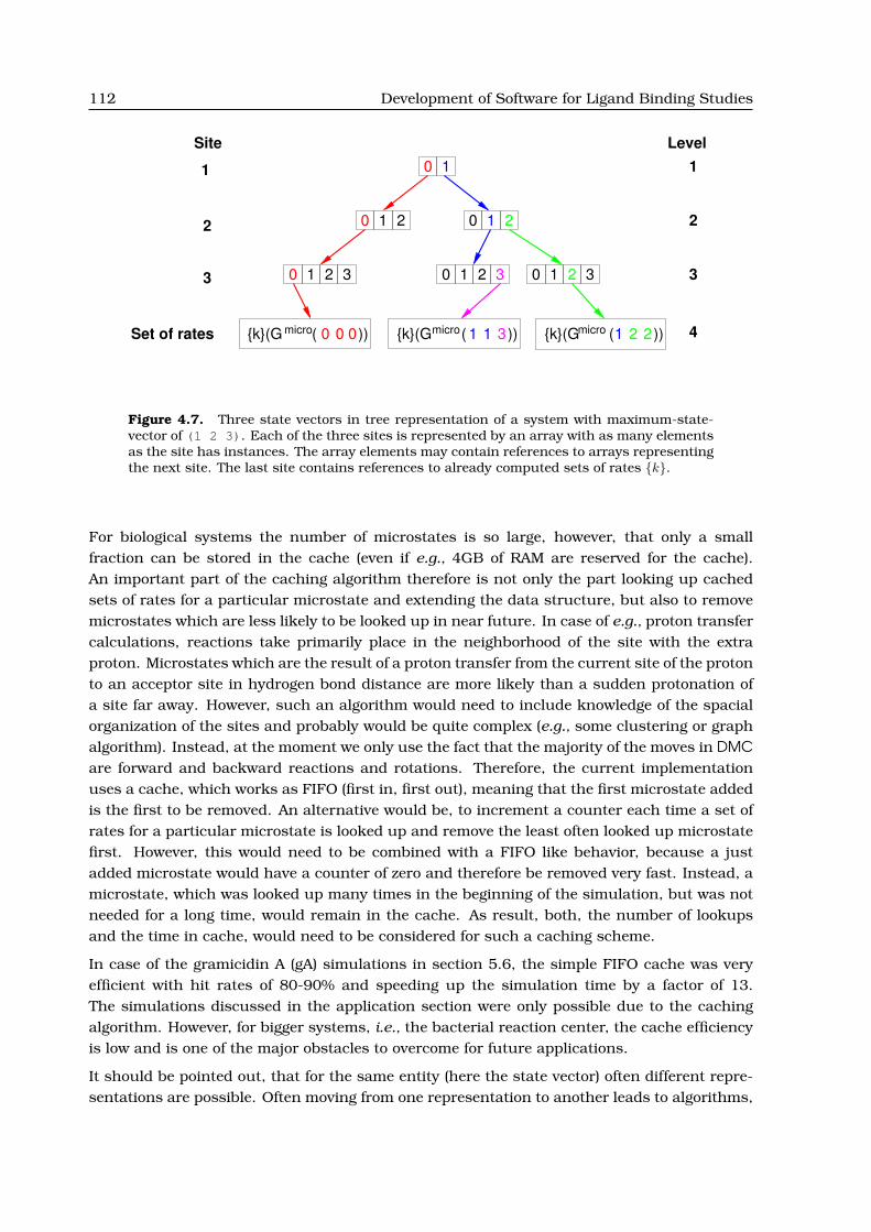
112 Development of Software for Ligand Binding Studies
0 1
1 20 0 1 2
1 2 30 10 2 3 10 32
Site
1
2
3
Set of rates
Level
4
3
2
1
micro 0 0 0{k}(G ( micro 1 1{k}(G ( 3 micro 1 2 2{k}(G ()) )) ))
Figure 4.7. Three state vectors in tree representation of a system with maximum-state-vector of (1 2 3). Each of the three sites is represented by an array with as many elementsas the site has instances. The array elements may contain references to arrays representingthe next site. The last site contains references to already computed sets of rates {k}.
For biological systems the number of microstates is so large, however, that only a smallfraction can be stored in the cache (even if e.g., 4GB of RAM are reserved for the cache).An important part of the caching algorithm therefore is not only the part looking up cachedsets of rates for a particular microstate and extending the data structure, but also to removemicrostates which are less likely to be looked up in near future. In case of e.g., proton transfercalculations, reactions take primarily place in the neighborhood of the site with the extraproton. Microstates which are the result of a proton transfer from the current site of the protonto an acceptor site in hydrogen bond distance are more likely than a sudden protonation ofa site far away. However, such an algorithm would need to include knowledge of the spacialorganization of the sites and probably would be quite complex (e.g., some clustering or graphalgorithm). Instead, at the moment we only use the fact that the majority of the moves in DMCare forward and backward reactions and rotations. Therefore, the current implementationuses a cache, which works as FIFO (first in, first out), meaning that the first microstate addedis the first to be removed. An alternative would be, to increment a counter each time a set ofrates for a particular microstate is looked up and remove the least often looked up microstatefirst. However, this would need to be combined with a FIFO like behavior, because a justadded microstate would have a counter of zero and therefore be removed very fast. Instead, amicrostate, which was looked up many times in the beginning of the simulation, but was notneeded for a long time, would remain in the cache. As result, both, the number of lookupsand the time in cache, would need to be considered for such a caching scheme.
In case of the gramicidin A (gA) simulations in section 5.6, the simple FIFO cache was veryefficient with hit rates of 80-90% and speeding up the simulation time by a factor of 13.The simulations discussed in the application section were only possible due to the cachingalgorithm. However, for bigger systems, i.e., the bacterial reaction center, the cache efficiencyis low and is one of the major obstacles to overcome for future applications.
It should be pointed out, that for the same entity (here the state vector) often different repre-sentations are possible. Often moving from one representation to another leads to algorithms,

4.2. Algorithms Contributed to Other Projects 113
which are much better suited for a particular purpose. In the example given here, the depen-dence of the algorithm with the number of microstates could be completely removed. In theapplication to gA, the system was modeled by 11 sites with 10 instances each (section 5.6).Instead of a search in 1011 microstates for an identical state vector, only 10 pointers need tobe dereferenced. Instead of - in the worst case - 1011 · 10 comparisons of elements of the cur-rent state vector with the elements of all possible state vectors in a complete cache, only 10comparisons are necessary, no matter how large the cache is.
4.2.3 Accelerating Titration Calculations using Adaptive Mesh Refinement
I developed an algorithm to speed up titration calculations, only afterwards noticing the pre-vious work by Berger, Oliger and Coella [138, 139], who developed a similar algorithm totrace particle movement in time. Their adaptive mesh refinement (AMR) algorithm becameimportant in the astrophysics, fluid dynamics and high-energy physics communities.
In section 3.1.3, the calculation of probabilities and equilibrium constants was described.It was pointed out, that an analytical evaluation of the partition function is only possiblefor small systems with not much more than 20 sites. Probabilities of such systems can becalculated, e.g., with the program SMT. For larger systems the probabilities have to be ap-proximated, e.g., by a Monte Carlo procedure (section 3.1.4) as implemented in the programGMCT. Usually, the probabilities for a known set of thermodynamic variables (i.e., chemi-cal potentials) are not the aim of the calculations, but the dependence of the probability onvarying chemical potentials. Therefore, the chemical potentials have to be scanned within areasonable range and the probabilities calculated at each point. For a fine resolution of thetitration curves, especially in the region were a particular site titrates, one needs to samplethe chemical potential range in fine steps. The number of points, at which the probabilitiesneed to be calculated increases exponentially with the number of chemical potentials takeninto account (number of ligand types in the calculation). Already for 1-dimensional protona-tion probability calculations on a small protein in a range of pH 0 to 14 with a step size of 0.1pH units and standard values for the number of MC scans and MC moves (section 3.1.4), theMonte Carlo titration is slower than the electrostatic calculations with QMPB. The discrepancyincreases exponentially with the number of ligand types (QMPB scales linear and GMCT scalesexponential).
The computational time of Perl Molecule and QMPB is in the order of seconds. The compu-tational effort of solving the PBE with the MEAD based helper programs scales with the totalnumber of instances of the system for a particular conformer i, where the total number ofinstances is the number of instances of each site Ninstance,i,l summed over all Nsite,i sites:
O
(Nsite,i∑l
Ninstance,i,l
)(4.1)
Each computation takes in the order of minutes per instance (but may be run in parallel). Thecomputational effort of the Monte Carlo titrations scales instead
O
(Nligand∏λ
(Nsite,i ·Nscans ·Nsteps,λ)), (4.2)

114 Development of Software for Ligand Binding Studies
-500
-450
-400
-350
-300
-250
-200
-150
-100
-50
0
E
0 2 4 6 8 10 12 14
pHC
PU
1
CP
U2
CP
U3
CP
U4
CP
U5
CP
U6
CP
U7
Figure 4.8. Speeding up titration calculations by splitting up chemical potential space.Each subrange of chemical potentials can be calculated on a different processor. In thisexample, the interesting part of the titration curve is only calculated by CPU4, while theother processors only calculate constant values.
so that each computation is in the order of 10 minutes for one ligand type λ (Nligand= 1). Theeffort however increases exponentially with the number of ligand types Nligand, that computa-tions with more than two or three ligand types become unfeasible.
The number of MC scans Nscans can not be reduced without reducing sampling quality andthe number of increments in chemical potential Nsteps,λ is defined by chemical potential rangeand step size. The step size needs to be sufficiently fine in regions where a site titrates.The number of sites Nsite,i in a conformer i depends on the system and equals the numberof MC moves Nmoves (section 3.1.4). Certainly, since the result for a given set of chemicalpotentials is calculated completely independent of the calculation for another set of chemicalpotentials, the calculations are embarrassingly parallel and can be easily split over manyprocessors (Fig. 4.8). However, by this method one can only expect a linear speedup, so thatthe wallclock time is divided by the number of processors used.
The adaptive mesh refinement (AMR) approach, however, tries to reduce the execution timedue to a better algorithm. The primary idea, is that most sites only titrate in a relatively smallregion of chemical potential space and they can be described by a single instance in largeregions of chemical potential space (Fig. 4.9).
If it would be known a priori, that a site only populates a single instance in a given regionof chemical potential space, all other instances could be excluded from the titration calcula-tions. Most sites bind only one (or a few) ligand types and do not interact strongly with sitesbinding other ligands (i.e., a protein with a redox site may have some protonateable residuessurrounding the redox site and they interact by electrostatics strongly, but protonateableresidues far away from the redox site are independent of the reduction potential and may onlydepend on the pH). Therefore, these sites titrate only in one dimension and are constant inthe other dimensions. Taking this fact into account could help reducing the number of pointsin chemical potential space, which are needed to describe the titration behavior of a particular

4.2. Algorithms Contributed to Other Projects 115
-500
-450
-400
-350
-300
-250
-200
-150
-100
-50
0
E
0 2 4 6 8 10 12 14
pH
A
-500
-450
-400
-350
-300
-250
-200
-150
-100
-50
0
E
0 2 4 6 8 10 12 14
pH
B
-500
-450
-400
-350
-300
-250
-200
-150
-100
-50
0
E
0 2 4 6 8 10 12 14
pH
C
Figure 4.9. Examples for titration curves. A: A protonateable site with only little depen-dence on the reduction potential. B: A redox site with a strong dependence on the pH. C:A site with different rotamer forms, which strongly depend on both the pH and reductionpotential. At low pH and reduction potential the instance plotted here is populated to about75% (cyan), at high pH and reduction potential it is only populated about 25% (yellow). Inthe other areas it is populated about 50%.
site. Therefore, such an algorithm could reduce the exponential scaling with number of ligandtypes to a scaling with lower power for most sites.
To introduce the AMR algorithm, Fig. 4.10 shows how an arbitrary step function of twovariables can be approximated. Given a computational method, which allows to calculatef(x, y) = z, where z is either zero (red) or one (blue), the function can be successively betterdescribed by partitioning space. Here, I chose to half the range of both variables in each step,so that squares (or rectangles) of decreasing sizes are obtained. In higher dimensions, spacewould be partitioned in cubes (or cuboids). Other geometrical forms (i.e., triangles) are pos-sible as well, but rectangles (or cuboids) are particularly easy to compute in cartesian space.Each time the step function has the same value at the four corner points of the rectangle (gen-erally 2Nligand vertices of the hypercube), the interior of the rectangle is assumed to be constantwith this value. The rectangle is excluded from further partitioning. As can be seen in thefigure, the algorithm approaches relatively fast to a mesh with fine resolution in the vicinity ofthe step. It is obvious from the figure, that the number of points of an equally spaced grid withthe same resolution as the finest mesh is much larger. Calculating all points on the equallyspaced grid would therefore require many more evaluations of the function f(x, y), which isassumed to be time consuming.
However, for a step function, AMR may lead to wrong results as shown in Fig. 4.10 H, whenthe function has critical points, which are closer than the coarsest grid. In most cases,such mistakes can however be seen, when critically inspecting the plots. For the applicationdiscussed here, the calculation of titration curves, the function is not a step function, but acontinuous function. The protonation probability is a real number between zero and one ateach point and the transition between the extrema has a finite width. One defines a tolerance(unimportant difference in probability), which is accepted for the vertices of the cube to varyand still considering the region as constant. For a given tolerance and assumed sigmoidaltitration behavior between the extrema, a chemical potential range can be estimated, which isconsidered safe (not to miss critical points) for the coarsest grid.
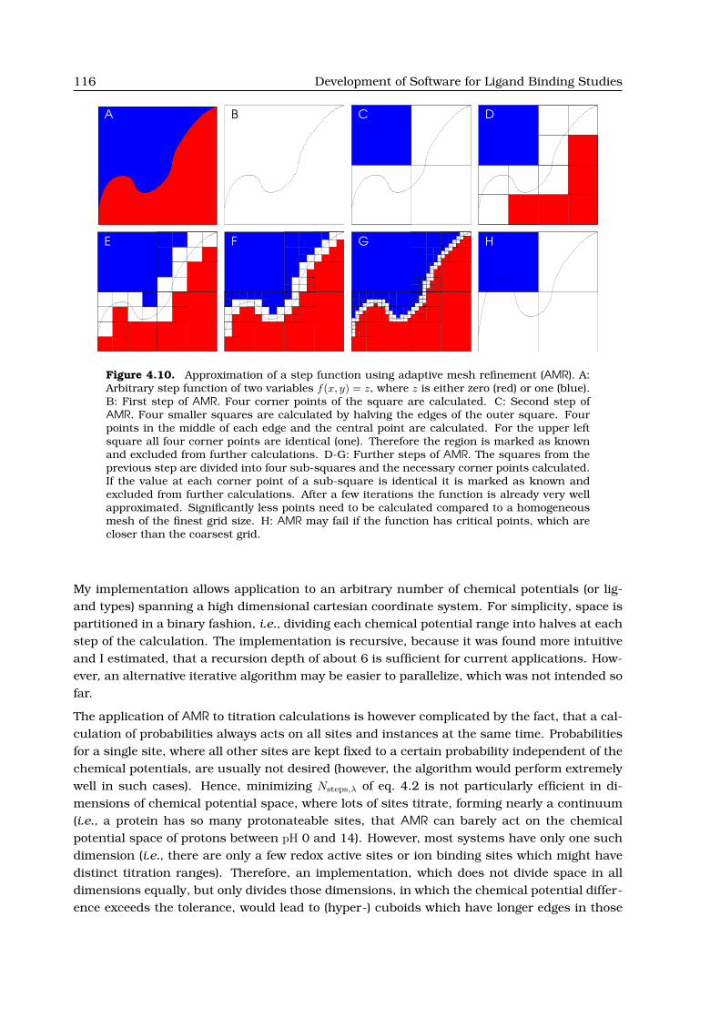
116 Development of Software for Ligand Binding Studies
A B C D
E F G H
Figure 4.10. Approximation of a step function using adaptive mesh refinement (AMR). A:Arbitrary step function of two variables f(x, y) = z, where z is either zero (red) or one (blue).B: First step of AMR. Four corner points of the square are calculated. C: Second step ofAMR. Four smaller squares are calculated by halving the edges of the outer square. Fourpoints in the middle of each edge and the central point are calculated. For the upper leftsquare all four corner points are identical (one). Therefore the region is marked as knownand excluded from further calculations. D-G: Further steps of AMR. The squares from theprevious step are divided into four sub-squares and the necessary corner points calculated.If the value at each corner point of a sub-square is identical it is marked as known andexcluded from further calculations. After a few iterations the function is already very wellapproximated. Significantly less points need to be calculated compared to a homogeneousmesh of the finest grid size. H: AMR may fail if the function has critical points, which arecloser than the coarsest grid.
My implementation allows application to an arbitrary number of chemical potentials (or lig-and types) spanning a high dimensional cartesian coordinate system. For simplicity, space ispartitioned in a binary fashion, i.e., dividing each chemical potential range into halves at eachstep of the calculation. The implementation is recursive, because it was found more intuitiveand I estimated, that a recursion depth of about 6 is sufficient for current applications. How-ever, an alternative iterative algorithm may be easier to parallelize, which was not intended sofar.
The application of AMR to titration calculations is however complicated by the fact, that a cal-culation of probabilities always acts on all sites and instances at the same time. Probabilitiesfor a single site, where all other sites are kept fixed to a certain probability independent of thechemical potentials, are usually not desired (however, the algorithm would perform extremelywell in such cases). Hence, minimizing Nsteps,λ of eq. 4.2 is not particularly efficient in di-mensions of chemical potential space, where lots of sites titrate, forming nearly a continuum(i.e., a protein has so many protonateable sites, that AMR can barely act on the chemicalpotential space of protons between pH 0 and 14). However, most systems have only one suchdimension (i.e., there are only a few redox active sites or ion binding sites which might havedistinct titration ranges). Therefore, an implementation, which does not divide space in alldimensions equally, but only divides those dimensions, in which the chemical potential differ-ence exceeds the tolerance, would lead to (hyper-) cuboids which have longer edges in those

4.2. Algorithms Contributed to Other Projects 117
Figure 4.11. Benchmarks of AMR with different tolerance values. The quality of thetitration curves is not much effected up to a tolerance of 30%, however the run-time canbe significantly reduced. A: full Monte Carlo, 100% run-time B: AMR with tolerance of 2%,80% run-time C: AMR with tolerance of 5%, 72% run-time D: AMR with tolerance of 10%,70% run-time E: AMR with tolerance of 30%, 54% run-time F: AMR with tolerance of 50%,49% run-time
dimensions, which are less crowded. Probably, other n-dimensional space filling tessellations(honeycombs) can be found, which faster approximate titration curves, however it has to beseen, if the computational effort to compute these polytopes does not slow down the AMRprocedure too much.
Another approach reducing the basis of eq. 4.2, is minimizing other factors, in particularNsite,i. The computational effort can be reduced by removing instances which are not popu-lated in the next coarser grid (therefore enhancing the sampling of the other instances). Inparticular for sites with many instances, it is often the case that only very few instances arein fact populated, but the other instances could not be excluded a priori. If a site is onlyrepresented by a single instance in a certain region of chemical potential space, the site canbe removed (by modifying the intrinsic energies of all other instances of all other sites bythe interaction energy with this instance) for finer grid calculations necessary for other sites.Removing sites reduces the length of the state vector (i.e., Nsite,i). In particular for calcu-lations including rotamers it is common, that (rotameric) instances adopt a fixed ratio overlarge ranges of chemical potential space (Fig. 4.9 C). The state vector length could be reducedby such sites using a mean-field approximation (calculating mean interaction energies as de-scribed in section 5.2). Furthermore, for short state vectors a statistical evaluation of thepartition function (by SMT) is more efficient than the Monte Carlo approximation scheme (inGMCT). The AMR algorithm can easily switch between the methods as soon as the state vectoris shorter than a pre-defined threshold value.

118 Development of Software for Ligand Binding Studies
Due to the multi-faced dependence of the performance of the algorithm on the system it wasnot possible to derive an analytical expression for the complexity of the algorithm. Two bordercases can be formulated: First, all instances are equally populated through space. Withoutmean-field approximation, this would lead to a complexity identical to eq. 4.2. Due to theoverhead of AMR some additional penalty would be added to the linear scanning of chemicalpotential space. Second, no instance is populated through space. It is sufficient to calculatethe vertices of the coarsest grid, i.e.,
O
(Nsite,i ·Nscans · 2Nligand
). (4.3)
More realistic scenarios perform between these two border cases. Very preliminary bench-marks of a test-implementation have shown, that a factor of two can easily be obtained fortwo dimensional titration calculations compared to sequential scanning of chemical potentialspace. In this test, space was partitioned in squares, not in probably more efficient rectangles.One dimension was the pH range of 0 to 14, which was covered to a large degree by protonate-able sites, so that AMR could not perform very well in this dimension. The second dimensionwas the reduction potential of a single site, however AMR could not take much advantage outof this fact due to the strictly squared (not rectangular) partitioning scheme. Therefore, it isvery likely, that AMR will perform much better with a rectangular partitioning scheme andmore, but less populated dimensions. The current implementation introduces a large over-head by using GMCT (and SMT) as external helper programs and generating new input filesfor each square. A significant performance impact can probably be gained by implementingthe algorithm together with the probability calculations in a single program (or using SWIG,section 4.4.4). However, interestingly the calculations have shown, that the tolerance can bechosen quite high (as 30%) without changing the titration curves significantly (Fig. 4.11), butreducing the run-time exponentially. The exponential dependence is probably due to the fact,that the ranges in which a site is considered to titrate get smaller. Therefore, larger squarescan be used to approximate the titration curves and less smaller cubes are needed.
Another limitation of the current implementation is, that an evenly spaced grid is used, ap-propriate for the finest mesh resolution. This choice was made to ease the implementation,which was focussed on saving processor time. However, one of the advantages of AMR, thereduced memory consumption, is not exploited. For three dimensions, 64 points of double (8byte) per dimension and 500 instances (in total) already 1GB of memory would be consumed.Since such a system is rather small, it can be estimated, that not unrealistic systems (fivedimensions, 128 points, 5000 instances) could easily require petabytes of memory - threeto four orders of magnitude beyond what is currently commonly available as disk space andfive to six orders of magnitude beyond what is currently available as memory. Therefore, ex-ploiting the conceptionally inherent memory saving capabilities of AMR using a sparse matrix(sparse tensor) or graph algorithm for storing probability values, may be as required for futureapplications as the processor time saving capabilities.
A project, which Eva-Maria Krammer already started, is the competitive binding of differentinhibitors instead of Coenzyme Q to the bacterial reaction center in addition to her studieson electron and proton binding to the protein and its cofactors. This application will requirenot only to include the chemical potentials of protons and electrons, but also of CoenzymeQ and its inhibitors into the ligand binding calculations. Titrations in such a four or higher

4.3. QMPB - A Program for Calculating Binding Energetics of Multiple Ligands 119
dimensional system will be very time-consuming and barely doable without AMR. Here, AMRis expected to perform much better, because only a few proton and electron binding sites inthe vicinity will depend on the cofactor or inhibitor being bound. Similarly, the binding ofinhibitors will only depend on the protonation or redox state of a few sites of the protein.
4.3 QMPB - A Program for Calculating Binding Energetics of
Multiple Ligands
QMPB allows to calculate intrinsic energies and interaction energies of sites with multipleinstances and multiple ligand types. It performs energy calculations based on the theory dis-cussed in chapter 3. Calculations for a particular site can be based on experimental resultson model compounds or on results of quantum chemical calculations. The flexibility of QMPBeven allows to combine sites of both types in a single calculation. Model compounds can befreely defined to optimally fit the experimental setup by the calculation. The current versionis able to deal with three dielectric regions, unlike Multiflex, which had only two. More dielec-tric regions are planned for the future. QMPB uses external helper programs (discussed insection 4.4) to solve the LPBE to calculate electrostatic energies.
4.3.1 Aims and General Concepts for the Development of QMPB
My primary aim when designing QMPB was to make it as transparent to the user as possible.Each step should be understandable and repeatable in small parts by the user. This trans-parency was felt to be necessary after having a more monolithic program, Multiflex, whichwas often used as a black box, sometimes leading to mistakes. Also the theory, introducedin chapter 3, needed to be tested carefully. The transparent and modular design allowedThomas Ullmann for example to replace the helper programs for the electrostatic calculationsby versions, which included a new membrane model and membrane potentials.
An important aim was also to provide linear scalability with the total number of instances,i.e., the number of independent PBE calculations, which need to be done to solve the prob-lem. Since these calculations are independent, the parallel execution on different processorsshould be possible. Because MEAD is the PBE solver primarily used in the group, it waschosen as basis to develop the helper programs discussed in section 4.4. Other PBE solversas APBS could be used, if someone desires and develops analogous helper programs. In fact,most of the processor time is spend by these helper programs, so that the runtime of QMPBitself is negligible. Therefore, to obtain a linear scaling with the number of processors, itwas sufficient to allow running the helper programs in parallel. Also it was not required towrite QMPB completely in C++ (as MEAD is written in), but to use the - especially for stringprocessing, which is a major part of QMPB - more convenient and flexible language Perl.
QMPB requests an input file in a rather general, human readable format. However, the inputfile will usually not be written by the user, because it can be very long for proteins withmany sites. Instead pre-processors (section 4.5 and section 4.6) should generate the inputfile, which should only be controlled and in exceptional cases modified or extended by theuser. The input file includes a large number of other files, mostly pqr-files containing thecoordinates and charges of instances. Also these files are generated by the pre-processor

120 Development of Software for Ligand Binding Studies
Stop
Startqmpb.in
pqr−files
pqr−files
fpt−fileogm−files
job.sh
my_2diel_solver
my_3diel_solver
pqr2SolvAccVol
Read input files
Write input for PB solver Read output of PB solver
Sum up and write output
out−files
yes noPreprocessor mode
run−qmpb
gintr.dat W.datqmpb.sum
Compute Nodes
Figure 4.12. Conceptional flowchart of QMPB. QMPB (green box) is called twice, oncein a pre-processor mode to set up the calculations by the PB solver programs (left half ofthe figure) and once to post-process the output files of the PB solver programs and writegintr.dat and W.dat (right half of the figure). The PB solver calculations can be done inparallel. run-qmpb splits up the job.sh shell script (generated by QMPB) and runs the partson different computers. The figures in this section are color coded (main program - green,site master - cyan, site - yellow, job.sh - pink).
programs. Therefore, a large part of the knowledge how to set up QMPB calculations properlybecame part of the pre-processors. This division leaves QMPB only with its core function toread and validate the input, prepare the helper programs to run, collect the output of thehelper programs and sum up the intrinsic energies according to the thermodynamic cycles insection 3. The intrinsic energies and the interaction energies are each written to a file, whichcan be read by other programs (e.g., GMCT, SMT, DMC) to perform the titration or (electron-or proton-) transfer calculations.
4.3.2 Overview of a Program Run
The considerations in section 4.3.1 lead to a three-step design: First, QMPB is run in a pre-processor mode (left half of Fig. 4.12). It reads the input file (qmpb.in and pqr-files) andgenerates the input for the helper programs solving the PBE (i.e., pqr-files, ogm-files for thegrid definition and a extended fpt-file to calculate the interaction energy). QMPB writes a shellscript (job.sh), doing calls to the helper programs (section 4.4).
Second, this shell script (job.sh) is executed. Optionally, the shell script can be split intoparts and submitted to different computers (i.e., via a queuing system of a compute cluster).

4.3. QMPB - A Program for Calculating Binding Energetics of Multiple Ligands 121
The approach chosen here completely separates off the questions concerning parallelizationand distributed computing. In QMPB no assumptions need to be made about the computingenvironment. Instead an external program can be adopted for the particularities of the site.Currently, an additional Perl program (run-qmpb) fulfills this function.
Third, QMPB is run in a post-processor mode (right half of Fig. 4.12). It reads the input file(qmpb.in and pqr-files) and the output files (out-files) generated by the helper programs.Intrinsic energies are computed according to the thermodynamic cycles in section 3. Threefiles are written: one for the intrinsic energies (gintr.dat), one for the interaction energies(W.dat) and a summary file (qmpb.sum). The summary file contains all the contributions tothe intrinsic energies and is usefull for the user to understand the calculations as they areperformed by QMPB.
4.3.3 The Input File
This section outlines the input file of QMPB placing emphasis on the general structure, closelyreflecting the object structure discussed in the next section, and leaving a full explanation foreach possible input option to appendix A.6. The aim of defining the input file format wasto allow access to the full functionality of QMPB. Since it was thought to be written by pre-processors, it was not important to be very compact. Instead it should be well readable bythe user to check and modify input options. The input is structured into a block with generaloptions and blocks for each instance of each site. The options are mostly given as key=value
pairs, where the value can sometimes be a space separated list of values. The order of theparameters in a block and the order of blocks is arbitrary. I refer to line numbers of thegiven examples in the following, however the line numbers are generally not important for theprogram. All energies are given in units of kcal
mol .
The General Block
The general block may contain options similar to the following example:
1 meadpath = /home/essigke/bin
2 T = 300
3 I = 0.1
4 backfi le = background . pqr
5 MGMcenter = ON CENT OF INTR
6 MGMpoints = 131
7 MGMspace = 0.2
8 OGMcenter = ON GEOM CENT ON CENT OF INTR
9 OGMpoints = 131 131
10 OGMspace = 1 0.2
11 epsin1 = 1
12 epsin2 = 4
13 Ligand Labels = proton electron
Line 1 in the example defines the path to the helper programs (section 4.4), then some param-eters for the Poisson-Boltzmann solver are given (absolute temperature T and ionic strengthI). Line 4 gives the name of the background pqr-file. It contains the coordinates, charges and
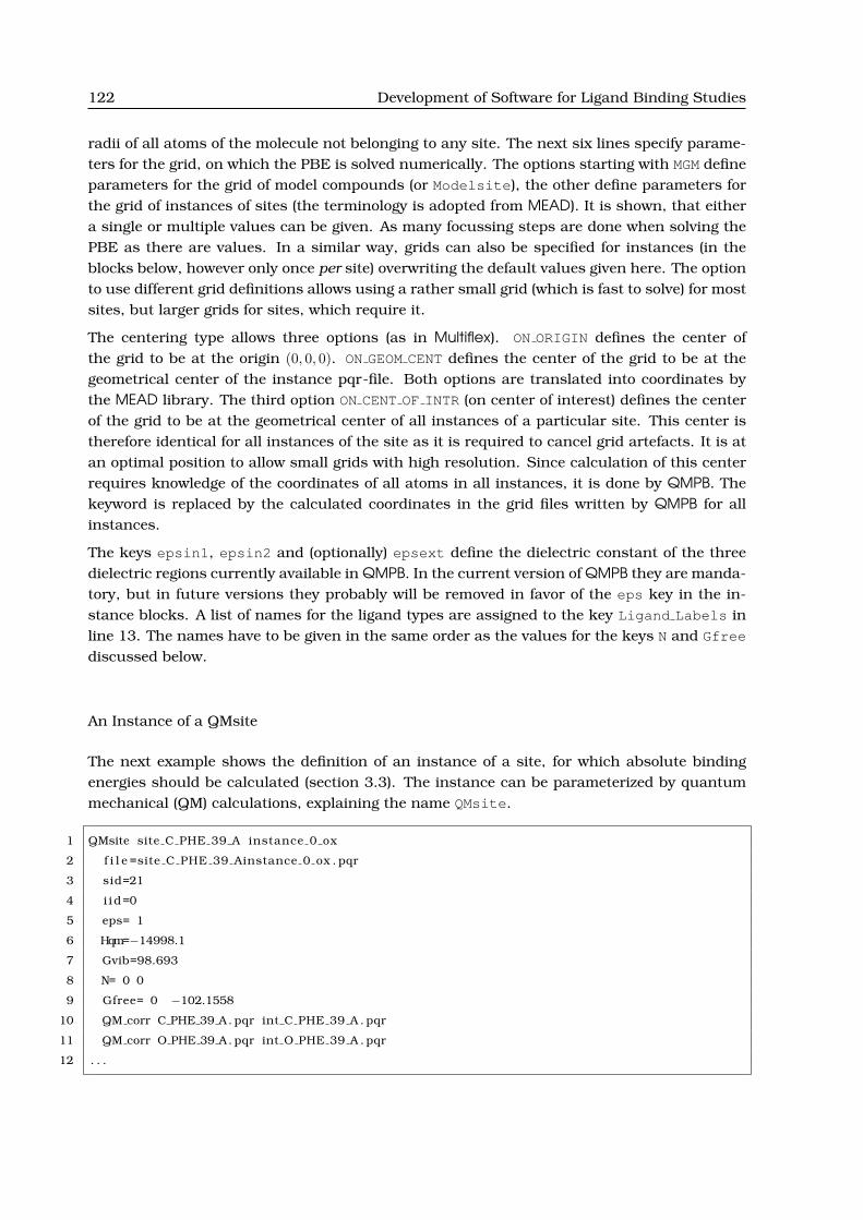
122 Development of Software for Ligand Binding Studies
radii of all atoms of the molecule not belonging to any site. The next six lines specify parame-ters for the grid, on which the PBE is solved numerically. The options starting with MGM defineparameters for the grid of model compounds (or Modelsite), the other define parameters forthe grid of instances of sites (the terminology is adopted from MEAD). It is shown, that eithera single or multiple values can be given. As many focussing steps are done when solving thePBE as there are values. In a similar way, grids can also be specified for instances (in theblocks below, however only once per site) overwriting the default values given here. The optionto use different grid definitions allows using a rather small grid (which is fast to solve) for mostsites, but larger grids for sites, which require it.
The centering type allows three options (as in Multiflex). ON ORIGIN defines the center ofthe grid to be at the origin (0, 0, 0). ON GEOM CENT defines the center of the grid to be at thegeometrical center of the instance pqr-file. Both options are translated into coordinates bythe MEAD library. The third option ON CENT OF INTR (on center of interest) defines the centerof the grid to be at the geometrical center of all instances of a particular site. This center istherefore identical for all instances of the site as it is required to cancel grid artefacts. It is atan optimal position to allow small grids with high resolution. Since calculation of this centerrequires knowledge of the coordinates of all atoms in all instances, it is done by QMPB. Thekeyword is replaced by the calculated coordinates in the grid files written by QMPB for allinstances.
The keys epsin1, epsin2 and (optionally) epsext define the dielectric constant of the threedielectric regions currently available in QMPB. In the current version of QMPB they are manda-tory, but in future versions they probably will be removed in favor of the eps key in the in-stance blocks. A list of names for the ligand types are assigned to the key Ligand Labels inline 13. The names have to be given in the same order as the values for the keys N and Gfree
discussed below.
An Instance of a QMsite
The next example shows the definition of an instance of a site, for which absolute bindingenergies should be calculated (section 3.3). The instance can be parameterized by quantummechanical (QM) calculations, explaining the name QMsite.
1 QMsite site C PHE 39 A instance 0 ox
2 f i l e =site C PHE 39 Ainstance 0 ox . pqr
3 sid=21
4 i id=0
5 eps= 1
6 Hqm=−14998.1
7 Gvib=98.693
8 N= 0 0
9 Gfree= 0 −102.1558
10 QM corr C PHE 39 A . pqr int C PHE 39 A . pqr
11 QM corr O PHE 39 A. pqr int O PHE 39 A . pqr
12 . . .

4.3. QMPB - A Program for Calculating Binding Energetics of Multiple Ligands 123
Line 1 specifies the type of site, a unique label for the site and a unique label for the instance.These labels should be intuitive for the user, facilitating a quick understanding of the inputand output files, where these labels are reused. Line 2 sets the name of the pqr-file, whichis defining the coordinates, charges and radii of atoms belonging to the instance of the site.Line 5 defines the dielectric constant of the region of the site. The optional keys sid andiid (line 3 and 4) associate the site and instance with unique numbers. They are usedfor sorting the output, which is usefull for post-processing scripts, but also comparison ofdifferent calculations. If the keys sid and iid are omitted, they are automatically generatedby QMPB. Line 6 and 7 define the quantum chemical energy of the instance (Hqm, total bondingenergy or energy of formation, Hvac,i(jk) in eq. 3.32) and the vibrational energy (Gvib, which isGvib,i(jk) in eq. 3.32), respectively. Line 8 and 9 give the number of bound ligands of each type(N, which is nλ,i(jk) in eq. 3.7 and eq. 3.34) and the standard chemical potentials for all ligandtypes (Gfree, which is µ◦λ in eq. 3.34). Line 10 and the following lines are for calculatingthe correction energy (Gcorr,i(jk) in eq. 3.32). Section 3.5.2 explains, why this correction isnecessary. The first pqr-file in each QM corr line specifies an atom in the QMsite (named Q1or Q2 in Fig. 3.7) and the second pqr-file specifies the atoms outside of this site, with which itartificially interacts (M1 and M2 in Fig. 3.7). Alternatively to the QM corr lines, a line with thekey Gcorr and the correction energy as value, can be given. Calculating the correction energyis very expensive and usually redundant in repetitive calculations.
An Instance of a MMsite - Non-Ligand Binding Reference Rotamer Form
Section 3.4 describes the calculation of energies of instances of sites relative to a reference.Four types of such instances were distinguished. The energy of the non-ligand binding ref-erence rotamer form is defined to be zero. Nevertheless, the electrostatic energy in the het-erogeneous environment of the molecule compared to a homogeneous dielectric is required bynon-reference rotamer forms. Therefore the energy is calculated.
1 MMsite s i te HT1 ALA 1 A instance 0 C
2 f i l e =s i te HT1 ALA 1 Ainstance 0 C. pqr
3 sid=0
4 i id=0
5 re f=se l f
6 eps= 4
7 N= 0 0
8 Gmm=0.3299
As for the QMsite, line 1 specifies the type of site, a unique label for the site and a uniquelabel for the instance. The name MMsite was chosen in contrast to QMsite. Often the energiesof rotamers of this type of site (given in line 8) are obtained from a molecular mechanics (MM)force field. Line 2-4 and 6-7 are analogous to the QMsite. The key ref in line 5 has the valueself, indicating that the reference instance of this instance is the instance itself, neitheranother MMsite nor a Modelsite.

124 Development of Software for Ligand Binding Studies
An Instance of a MMsite - Non-Ligand Binding Non-Reference Rotamer Form
The next example shows the input for an instance, which takes the previous example asreference rotamer:
1 MMsite s i te HT1 ALA 1 A instance 1 A
2 f i l e =s i te HT1 ALA 1 Ainstance 1 A. pqr
3 sid=0
4 i id=1
5 re f=instance 0 C
6 Gmm=0.3355
The key ref in line 5 now has the value instance 0 C, which is the instance label of theprevious example instance. By that the program knows, that it should use instance 0 C
as reference instance for instance 1 A. The rotamer energy in line 6 is different from thereference instance. Note, that certain keys can only be given to the reference instance, not tonon-reference instances.
An Instance of a MMsite - Ligand Binding Reference Rotamer Form
In the previous examples, instances of type MMsite only differed in their coordinates (rotamerform), not in the number of ligands bound (charge form). In this case, the ligand bindingis described by a model compound in solution, for which ligand binding energies are known(e.g., from experiment).
1 MMsite s i te CE LYS 4 A instance 0 p ROT −5
2 f i l e =s i te CE LYS 4 Ainstance 0 p ROT −5.pqr
3 sid=1
4 i id=0
5 re f=model instance 0 p ROT −5
6 Gmm=0.0316
The key ref in line 5 now has the value model instance 0 p ROT -5, which is the instancelabel of the instance of a Modelsite. If the site only exists in a single rotamer form, the optionnohomo should be given for the MMsite. This option avoids the calculation of the instance ina homogeneous dielectric, which is only needed for rotamers.
An Instance of a Modelsite
The next example shows how to specify a model compound:
1 Modelsite s i t e CE LYS 4 A model instance 0 p ROT −5
2 f i l e =model s i t e CE LYS 4 Ainstance 0 p ROT −5.pqr
3 sid=1
4 i id=0
5 re f=instance 0 p ROT −5
6 Gmodel=−14.2665506152
7 eps= 4
8 N= 1 0

4.3. QMPB - A Program for Calculating Binding Energetics of Multiple Ligands 125
The input is very similar to a non-ligand binding reference rotamer form of a MMsite. Thetype of site is now Modelsite. A rotamer energy Gmm is not specified, because it is specifiedfor the associated MMsite given by the key ref. Instead, the energy of the model compound insolution is specified with the key Gmodel. It is important, that all Modelsite instances of a site(due to different charge forms) are in the same rotamer form. The file specifying the Modelsitehas to contain all atoms (with identical coordinates, charges and radii) as the associatedMMsite, but usually contains additional atoms, which were present when determining themodel energy in solution. The dielectric boundaries are calculated from all atoms in thisfile. The additional atoms contribute with their charges as background charge set to theelectrostatic energy.
An Instance of a MMsite - Ligand Binding Non-Reference Rotamer Form
Finally, there might be rotamer form, which takes a ligand binding rotamer form as reference:
1 MMsite s i te CE LYS 4 A instance 1 p ROT 24
2 f i l e =s i te CE LYS 4 Ainstance 1 p ROT 24.pqr
3 sid=1
4 i id=1
5 re f=instance 0 p ROT −5
6 Gmm=0.6172
The input is analogous to a non-ligand binding non-reference rotamer form, but the key ref
now points to instance instance 0 p ROT -5. The distinction, necessary for the differentcalculation schemes can only be made by analyzing the ref value of the reference instance.If it is self it is a non-ligand binding non-reference rotamer form, instead if a Modelsite
instance is specified, it is a ligand binding non-reference rotamer form.
4.3.4 The job.sh Script
From the input file QMPB produces a file job.sh, when it is run in pre-processor mode. Hereare the lines defined by the input blocks given as examples above (splitted lines are markedby a backslash):
1 #!/ bin/sh
2 /home/essigke/bin/pqr2SolvAccVol epsin1 region > pqr2SolvAccVol epsin1 region . out
3 /home/essigke/bin/pqr2SolvAccVol epsin2 region > pqr2SolvAccVol epsin2 region . out
4 /home/essigke/bin/my 3diel solver −eps1set epsin1 region −eps2set epsin2 region −T 300 \
5 −ionicstr 0.1 −epsin1 1 −epsin2 4 −fpt s i t e −epshomo 1 site C PHE 39 A instance 0 ox \
6 background > site C PHE 39 A instance 0 ox . out
7 /home/essigke/bin/my 3diel solver −eps1set epsin1 region −eps2set epsin2 region −T 300 \
8 −ionicstr 0.1 −epsin1 1 −epsin2 4 C PHE 39 A int C PHE 39 A > C PHE 39 A . out
9 /home/essigke/bin/my 3diel solver −eps1set epsin1 region −eps2set epsin2 region −T 300 \
10 −ionicstr 0.1 −epsin1 1 −epsin2 4 O PHE 39 A int O PHE 39 A > O PHE 39 A. out
11 . . .
12 /home/essigke/bin/my 3diel solver −eps1set epsin1 region −eps2set epsin2 region −T 300 \
13 −ionicstr 0.1 −epsin1 1 −epsin2 4 −fpt s i t e −epshomo 4 site HT1 ALA 1 A instance 0 C \
14 background > site HT1 ALA 1 A instance 0 C . out

126 Development of Software for Ligand Binding Studies
15 /home/essigke/bin/my 3diel solver −eps1set epsin1 region −eps2set epsin2 region −T 300 \
16 −ionicstr 0.1 −epsin1 1 −epsin2 4 −fpt s i t e −epshomo 4 site HT1 ALA 1 A instance 1 A \
17 background > site HT1 ALA 1 A instance 1 A . out
18 . . .
19 /home/essigke/bin/my 3diel solver −eps1set epsin1 region −eps2set epsin2 region −T 300 \
20 −ionicstr 0.1 −epsin1 1 −epsin2 4 −fpt s i t e −epshomo 4 \
21 site CE LYS 4 A instance 0 p MAX ROT −5 background > \
22 site CE LYS 4 A instance 0 p MAX ROT −5.out
23 /home/essigke/bin/my 2diel solver −epsin 4 −T 300 −ionicstr 0.1 \
24 site CE LYS 4 A instance 0 p MAX ROT −5 \
25 site CE LYS 4 A model instance 0 p MAX ROT −5 back2d > \
26 site CE LYS 4 A instance 0 p MAX ROT s−5 2d . out
27 /home/essigke/bin/my 3diel solver −eps1set epsin1 region \
28 −eps2set epsin2 region −T 300 −ionicstr 0.1 −epsin1 1 −epsin2 4 −fpt s i t e \
29 −epshomo 4 site CE LYS 4 A instance 1 p MAX ROT 24 background > \
30 site CE LYS 4 A instance 1 p MAX ROT 24 . out
31 . . .
The first two lines calculate the analytical surface representation for the two dielectric re-gions of the QMsite instances (epsin1 region) and protein (epsin2 region) including thebackground.pqr file and all QMsite and MMsite instances using the helper program Pqr2-SolvAccVol. More detailed information on the calculation of analytical surfaces and properboundary definitions is given in section 4.4.1.
Lines 4-10 show the calculation steps invoked by the given input fragment for an instanceof a QMsite. The first call of My 3Diel Solver (section 4.4.2) calculates the Born energy of theinstance in the three dielectric environment defined by the two solute regions epsin1 region
and epsin2 region and the solvent. Additionally, the Born energy is calculated in a homo-geneous dielectric of one (vacuum), due to the epshomo parameter. The background energy iscalculated as the interaction of the electrostatic potential of the instance with all charges in thebackground.pqr file. Additionally, interaction energies are calculated for all atoms of all in-stances of all other sites according to the extended fpt-file site.fpt generated by QMPB. Thefile format is described in appendix A.1.5. All energy contributions are stored in the output fileof My 3Diel Solver. To calculate the energy correction discussed in section 3.3.1, the next callsof My 3Diel Solver are made. The same boundary definitions as before are used, but the twopqr-files are those given by the QM corr option in the input file. Here, only the backgroundenergy due to the interaction of the electrostatic potential of the atom in the first pqr-fileϕprotein(~ra,i; qa,i(jk)) with the charges of the atoms Qprotein,A,i in the second pqr-file is of interest.Therefore, it is neither necessary to do a vacuum calculation to cancel grid artefacts in theBorn energy (by the option epshomo as in line5), nor interaction energy calculations accordingto an extended fpt-file (by the option fpt as in line 5). Lines 12-17 call My 3Diel Solver twiceto calculate the rotamer instances of a MMsite without model compound. Except that thecalculation in the homogeneous dielectric is done with the dielectric constant of the protein,the program calls are analogous to the calculation of the QMsite instance. Lines 19-30 showthe calculations for the MMsite with model compound. Again, the calls of My 3Diel Solver areanalogous. However, for the instance of the model compound My 2Diel Solver (section 4.4.3)is called. Since for every site the model compound has different dielectric boundaries they are

4.3. QMPB - A Program for Calculating Binding Energetics of Multiple Ligands 127
not calculated with Pqr2SolvAccVol in advance. The first pqr-file is identical in the calculationof the associated MMsite and in the calculation on the model compound. The second pqr-filecontains all atoms, which were present in the file specified in the QMPB input, but the chargesof the atoms found in the pqr-file of the MMsite are set to zero to calculate the backgroundenergy.
4.3.5 The Output Files
In a third step, after generation and execution of the job.sh script, QMPB is run in post-processor mode. The input file and all the output files generated by the helper programsare read. The electrostatic energy terms are extracted from the output files and properlyadded with the energies specified in the QMPB input file according to the equations given inchapter 3. The file qmpb.sum contains all energy contributions to the intrinsic energy in areadable format. For the example instance of a QMsite, page 122, the following informationis given:
1 s i te C PHE 39 A instance 0 ox
2
3 Born Energy :
4 Site in ThreeDielectric 15283.6
5 Site in Homogeneous Die lectr ic 15439.8
6 Difference : −156.199999999999
7 Background Energy :
8 Site in ThreeDielectric −21.6103
9
10 QM Energies :
11 Total Bonding Energy : −14998.1
12 Vibrational Energy : 98.693
13 Energy of free ligands : −102.1558 (2 ligand types )
14
15 Error correction for 1−2 and 1−3 interaction with protein : −47.5910176
16
17 Sum: −15131.7820824
The Born energy was calculated in a homogeneous and three dielectric environment (lines5 and 4). The given energies contain grid artefacts, which are canceled by calculating thedifference (line 6). The background energy in the three dielectric environment is given (line8). This energy contains the artefacts due to bonded and angle interactions which shouldbe excluded. The correction energy is given in line 15 and subtracted from the sum. Thequantum mechanical energy contributions (bonding energy, line 11 and vibrational energy,line 12) as well as the energy of free ligands (line 13) were given in the input file. Finally, allcontributions are summed up and the intrinsic energy is given (line 17).
Next, the calculation on two rotamer forms by instances of a MMsite was discussed on pages123–124. The qmpb.sum file gives the following information:
1 s i te HT1 ALA 1 A instance 0 C
2
3 Reference Rotameric Form without Modelsite !

128 Development of Software for Ligand Binding Studies
4
5 Born Energy :
6 Site in ThreeDielectric 137.608
7
8 Background Energy :
9 Site in ThreeDielectric 0.653352
10
11 Intr ins ic Model Energy : 0
12
13 Sum of contributions : 0
14 s i te HT1 ALA 1 A instance 1 A
15
16 Born Energy :
17 Site in ThreeDielectric 129.958
18 Site in Homogeneous Die lectr ic 146.483
19 Site in ThreeDielectric in reference rotameric form 137.608
20 Site in reference rotameric form in homogeneous d ie l ec t r i c 154.142
21 Difference 0.00899999999998613
22
23 Background Energy :
24 Site in ThreeDielectric 0.505013
25 Site in ThreeDielectric in reference rotameric form0.653352
26 Difference −0.148339
27
28 Molecular Mechanics Energy :
29 Site 0.3355
30 Site in reference rotameric form 0.3299
31 Difference 0.00559999999999999
32
33 Sum of contributions : −0.133739000000014
Lines 1 to 13 describe the reference rotamer instance. By definition the intrinsic energy iszero. However, for the non-reference rotamer instance (lines 14 - 33) the calculated Bornand background energies are given for both instances. Double differences in Born (line 21),differences in background (line 26) and differences in rotamer energies (line 31) are calculatedand summed up. Line 33 gives the intrinsic energy of the non-reference instance.
Finally, here are the lines of the qmpb.sum file referring to the two instances of the MMsite
with model compound (pages 124–125):
1 s i te CE LYS 4 A instance 0 p MAX ROT −5
2
3 Reference Rotameric Form!
4
5 Born Energy :
6 Site in ThreeDielectric 129.152
7 Modelsite in TwoDielectric 128.427
8 Difference 0.724999999999994

4.3. QMPB - A Program for Calculating Binding Energetics of Multiple Ligands 129
9
10 Background Energy :
11 Site in ThreeDielectric −0.746759
12 Modelsite in TwoDielectric −0.774909
13 Difference 0.02815
14
15 Intr ins ic Model Energy : −14.2665506152
16
17 Sum of contributions : −13.5134006152
18 s i te CE LYS 4 A instance 1 p MAX ROT 24
19
20 Born Energy :
21 Site in ThreeDielectric 216.191
22 Site in Homogeneous Die lectr ic 234.968
23 Modelsite in reference rotameric form 128.427
24 Site in reference rotameric form in homogeneous d ie l ec t r i c 148.139
25 Difference 0.935000000000031
26
27 Background Energy :
28 Site in ThreeDielectric −0.741824
29 Modelsite in TwoDielectric −0.774909
30 Difference 0.0330849999999999
31
32 Intr ins ic Model Energy : −14.2665506152
33
34 Molecular Mechanics Energy :
35 Site 0.6172
36 Site in reference rotameric form 0.0316
37 Difference 0.5856
38
39 Sum of contributions : −12.7128656152
Line 1 to 17 and line 18 to 39 give the energy contributions of the two instances of theMMsite. The Modelsite is not mentioned in a separate section, but their energies are givenin the sections of each instance, where they are needed for the calculation. For the referenceMMsite (line 1 - 17) the intrinsic energy (line 17) is calculated as sum of the energy of themodel compound (line 15) and the difference in Born and background energy (line 8 and13, respectively) between the instance and the model instance. For the non-reference rotamerinstance (line 18 - 39), the double difference in Born energy (line 25) is calculated according toeq. 3.41 and the difference in background energy (line 30) is calculated according to eq. 3.42,which can be derived form Fig. 3.9. The difference in rotamer energy (line 37) is calculatedand the terms are summed up to obtain the intrinsic energy (line 39)
The intrinsic energies are tabulated in the file gintr.dat:
1 # siteID instID s i te labe l inst label intr ins ic energy proton electron
2 1 1 s i te HT1 ALA 1 A instance 0 C 0.000 0 0
3 1 2 s i te HT1 ALA 1 A instance 1 A −0.134 0 0

130 Development of Software for Ligand Binding Studies
4 2 1 s i te CE LYS 4 A instance 0 p MAX ROT −5 −13.513 1 0
5 2 2 s i te CE LYS 4 A instance 1 p MAX ROT 24 −12.713 1 0
6 . . .
7 22 1 s i te C PHE 39 A instance 0 ox −15131.782 0 0
The first two columns give the site and instance number (sid and iid) incremented by oneas it is required for SMT and GMCT. QMPB usually starts counting at zero (as in the input file)and gives these numbers also as default output format. The next two columns give the siteand instance label as they were given in the input file. The fifth column contains the intrinsicenergy and all following columns give the number of bound ligands for each ligand type.
The third output file W.dat contains all the interaction energies (each line had to be splittedover two lines):
1 # siteID1 instID1 si te lab1 instlab1 \
2 siteID2 instID2 si te lab2 instlab2 symmetrized energy interaction energy error
3 1 1 s i te HT1 ALA 1 A instance 0 C \
4 1 1 s i te HT1 ALA 1 A instance 0 C 0.000 0.000 0.000
5 1 1 s i te HT1 ALA 1 A instance 0 C \
6 1 2 s i te HT1 ALA 1 A instance 1 A 0.000 0.000 0.000
7 . . .
8 1 1 s i te HT1 ALA 1 A instance 0 C \
9 2 1 s i te CE LYS 4 A instance 0 p MAX ROT −5 0.108 0.109 0.001
10 1 1 s i te HT1 ALA 1 A instance 0 C \
11 2 2 s i te CE LYS 4 A instance 1 p MAX ROT 24 0.110 0.110 0.000
12 . . .
13 1 1 s i te HT1 ALA 1 A instance 0 C \
14 22 1 s i te C PHE 39 A instance 0 ox −0.053 −0.053 0.000
15 . . .
The W.dat file contains the pairwise interaction energies of each instance (specified by siteand instance number and site and instance label) with each other instance (specified by thesame four attributes). The calculated interaction energy is given in column 10. Since eachinteraction energy is calculated twice (as electrostatic potential of site 1 times charge of site2 and electrostatic potential of site 2 times charge of site 1) this redundancy can be used forerror estimation. The symmetrized interaction energy (column 9) is the arithmetic average ofthe two interaction energies and the error (column 11) is the difference between the interactionenergy and the symmetrized interaction energy.
4.3.6 Hierarchy and Collabortation of Objects
QMPB uses the object-oriented programming (OOP) paradigm to structure the code internally.As mentioned in section 4.1, QMPB has an abstract site class. From this abstract classQMsite, MMsite and Modelsite classes are derived (Fig. 4.13). The advantage of the ab-stract definition of a site is that all common properties of the three derived classes can beimplemented at a central place and be used and potentially modified by the derived classes.These classes are instantiated, generating an object for each instance of a site. To manageall the site objects I developed a class called site master. It provides methods to the main

4.3. QMPB - A Program for Calculating Binding Energetics of Multiple Ligands 131
program for the different steps of the QMPB calculation. The methods usually delegate thework to appropriate methods of the site class. Due to the OOP approach, the site master
class does not need to differentiate between objects of type QMsite and MMsite, but can in-stead rely that the object will act according to its type, e.g., if the method print G is invoked,due to the polymorphism different methods are called and the energy is computed differentlyfor QMsite and MMsite objects. The sequence of the different calculation steps is shown inFig. 4.14. Additionally, there is a pqr class, which encapsulates the contense of a pqr-file inan object. It allows reading, writing and limited modification of pqr-files. The pqr objects areoften helper objects for objects derived from one of the site classes.
The site master class
The site master class represents a QMPB calculation on a single conformer. Objects areconstructed by the method read input, which takes a QMPB input file as most importantparameter (Fig. 4.14). The input file is parsed and objects of the other classes are constructedaccording to the input file. A major part of the code in the site master object is dedicatedto these two steps. Other public methods, i.e., methods accessed by the main program,are write MEAD and read MEAD, which generate the input for and reads the output file ofthe MEAD based helper programs (section 4.4). In fact, site master only iterates over thegenerated site objects and triggers them to do the write and read operations for their partic-ular instance. The method write output generates the output files gintr.dat, W.dat andqmpb.sum also by initiating each instance to write its data into the files.
The site class
The site class is an abstract base class for the QMsite, MMsite or Modelsite classes (Fig. 4.13).It implements methods common to instances of all types of sites. The constructor new takesa hash with the options given for the instance as parameter. This hash is previously filledby the input file parsing routines of site master. The constructor does the validation forthe options, which are common to all sites. Each derived class overwrites the constructorto include validation for the options particular to its class. The constructor also generates apqr object from the filename given in the input file, describing the coordinates, charges andradii of atoms belonging to this instance. The methods write job and read job are calledby site master write MEAD and read MEAD (Fig. 4.14). Besides a number of accessor andhelper methods, the class implements the abstract method print G, which is supposed to beoverwritten implementing the calculation of the intrinsic energy and the generation of appro-priate lines for the qmpb.sum and gintr.dat files for each derived class. The method print W
implements the generation of the instance specific part of the W.dat file.
The QMsite class
Objects of the QMsite class represent instances of a site, for which the intrinsic energy (sec-tion 3.3) should be calculated based on parameters obtained by quantum chemical methods.The constructor checks for the QMsite specific options, i.e., the quantum mechanical energy(Hqm), the vibrational energy (Gvib) and an array of standard chemical potentials for all ligandtypes (Gfree). Optionally, a correction energy (Gcorr) can be defined or calculated from a

132 Development of Software for Ligand Binding Studies

4.3. QMPB - A Program for Calculating Binding Energetics of Multiple Ligands 133
set of pqr-files given in the input following the tag QM corr. The method write job calls themethod of the site class and extends it with calls to the helper program My 3Diel Solver foreach pqr-file specified using the QM corr tag. The method read job similarly calls the methodof the site class and extends it by reading all the output files generated by the additional cal-culations and by calculating the correction energy. The method print G implements eq. 3.32and eq. 3.34 to calculate the absolute intrinsic energy.
The MMsite class
Objects of the MMsite class represent instances of a site, for which the relative intrinsic energyshould be calculated. The constructor checks for the rotamer energy (Gmm). Section 3.4 andsection 4.3.3 distinguished four different types of instances, which are all described by thissingle class. The distinction between the four types is done according to the value of theref key in the QMPB input file as discussed before. In the program, the instance labelsare replaced by references (pointers) to the appropriate objects. During the calculation ofthe intrinsic energy by the method print G, the references are used for calling the accessormethods of the reference site. Also the calculation scheme depends on the type of referenceand sometimes on the type of the reference of the reference object. If the MMsite objectrepresents a reference instance with model compound, it (mostly) manages its associatedModelsite object by itself after construction by the site master object. Therefore somemethods are extended compared to the site class.
The Modelsite class
Objects of the Modelsite class represent instances (in particular charge forms) of model com-pounds used by MMsite objects to calculate energies based on experimental model energies(Gmodel) and heterogeneous transfer energies. The electrostatic energy of a model compoundsis calculated in a two dielectric environment using the helper program My 2Diel Solver, notMy 3Diel Solver as it is used for QMsite and MMsite objects. Therefore the method write job
is overwritten. The background pqr-file as well as the dielectric boundaries are particular foreach Modelsite. Due to the different program and the background energy term the methodread job is also overwritten. The method print G is not implemented, since Modelsite ob-jects do not contribute directly to the output files. Instead, print G of the associated MMsite
Figure 4.13. Class diagram of QMPB including attributes and methods. The site masterclass (cyan) is a container class, which manages objects derived from the site class (1 −∗ association with a site class, instantiate dependency with derived classes). The siteclass is an abstract base class, which contains the common attributes and methods ofsites (generalization). QMsite, MMsite and Modelsite classes are derived from the siteclass. The QMsite class has some attributes specific for instances of quantum chemicallyparameterized sites, e.g., Hqm stores Hvac,i(jk) (section 3.3). The intrinsic energy is computedin print G according to eq. 3.32. Instead, the MMsite class implements print G to computeeq. 3.37. Dependent, if ligands are bound or if it is a non-ligand binding site, the MMsitemay use a Modelsite object to represent the instance of the site in the model compoundenvironment (1− 0 . . . 1 association). Both, the site master and the site class use the pqrclass as helper class to represent pqr-files (use dependency). The figures in this section arecolor coded (main program - green, site master - cyan, site - yellow, job.sh - pink).

134 Development of Software for Ligand Binding Studies
read input
write MEAD
new
run job.sh
print G
print W
write output
read MEAD
gintr.dat and
qmpb.sum
are produced
write job
read job
QMPB input
is read
job.sh
is written
MEAD output
is produced
MEAD output
is read
W.dat
is produced
masterjob.sh
:site_objects:site
program:main
sequence diagram QMPB
loop s (0,total number of instances)
loop s (0,total number of instances)
loop s (0,total number of instances)
loop s (0,total number of instances)
Figure 4.14. Sequence diagram of a QMPB run. The main program is slightly differenthere, since it runs in a single step the pre-processor part, the job.sh script and the post-processor part. Unlike the version discussed in the rest of the work, it is slightly simpler,but does not allow parallel execution of the job.sh script. The order of the method calls ofthe site master object as well as the calls to the polymorphic methods of all the QMsiteand MMsite objects are specified. The steps were input and output files are produced andprocessed are specified. The figures in this section are color coded (main program - green,site master - cyan, site - yellow, job.sh - pink).

4.4. Extensions to the MEAD Library and Suite of Programs 135
object accesses the energies via provided accessor methods and includes them into the calcu-lation.
The pqr class
Objects of the pqr class are an object-oriented representation of a pqr-file. The objects areusually constructed by reading a pqr-file. The class provides a number of methods to accessthe data, for example get charge returns the total charge of the pqr-file, get coord returnsall coordinates as (x, y, z)-triples or coord exists checks if an atom with given coordinatesis present in the pqr-file. The data can be manipulated (e.g., delete atom deletes a speci-fied atom or set charge sets the charge of a specified atom to a given value). Finally, themanipulated data can be written to a pqr-file again.
4.4 Extensions to the MEAD Library and Suite of Programs
Donald Bashford developed an object-oriented library for Molecular Electrostatics at AtomicDetail (MEAD [30]), i.e., a Poisson-Boltzmann solver suited for biological applications. Heprovides a number of programs based on this library, i.e., Solvate and Solinprot to calculatehomogeneous transfer energies (section 3.2.5) into a two dielectric environment or a threedielectric environment, respectively, and Multiflex to do relative pKa calculations (involvingcalculations of heterogeneous transfer energies, section 3.2.6). The theory underlying Multi-flex in comparison to QMPB is discussed in section 3.5. For QMPB the available programswere not suited. Therefore, the programs Pqr2SolvAccVol, My 3Diel Solver and My 2Diel Solverwere developed as helper programs for QMPB (section 4.4.1, section 4.4.2 and section 4.4.3,respectively). Calls of these programs with proper command line parameters and input filesare written to the file job.sh in the pre-processor run of QMPB. The output files of the helperprograms are parsed in the post-processor run of QMPB to obtain the electrostatic energies.Besides, these additions to MEAD a number of further extensions were made, which are sum-marized in section 4.4.5.
4.4.1 Dielectric Boundary Calculations with Pqr2SolvAccVol
To define the boundaries between dielectric regions, solvent accessible surfaces have to becalculated. This process is rather slow for complicated molecules with many atoms. MEADimplements an algorithm to calculate analytical surface representations [70]. From the ana-lytical surface, a grid representation can be calculated according to the parameters given forthe grid. The analytical representation is independent of grid parameters, so that the sameanalytical surface can be used to discretize grids of different center, size and resolution forfocussing steps or for different sites. This discretization is very fast compared to the analyticalsurface calculation.
For each conformation in QMPB, all instances of all sites have to be calculated with identicaldielectric boundaries. My 3Diel Solver is run independently for each instance. If the analyticalrepresentation of the surface would be calculated at each run, it would noticeably contributeto the overall runtime. Therefore, Pqr2SolvAccVol was written, which takes the coordinates

136 Development of Software for Ligand Binding Studies
of all atoms belonging to a dielectric region (in form of a pqr-file), calculates the analyticalrepresentation of the solvent accessible volume and writes it to disk. Runs of My 3Diel Solvercheck if a file is present containing the analytical surface representation and read it insteadof calculating the surface. The SolvAccVol class of MEAD provides methods to read and writethe analytical surface in plain text or binary format, but so far no program was using thesemethods.
It is important for the discretization step, that the surfaces are calculated properly. If thecoordinates used to define the analytical volume contain cavities, which are large enoughfor a water molecule, MEAD assigns the grid points in the volume of the cavity the dielectricconstant of the solvent. This feature is required for water filled cavities in proteins. However,when molecules are described by more than two dielectric regions this feature can lead tomistakes. For example, having a QMsite defining a dielectric region, the protein region andthe aqueous solution, one may calculate the region of the QMsite by the atoms belonging toinstances of this site and the protein region by all other atoms of the protein. This would leadto a cavity in the protein volume, where the QMsite is located. Since the solvent accessiblesurface algorithm calculates in one case an outer surface of the QMsite, but in the other casean inner surface according to the protein atoms, the two surfaces are not identical. Whencombining the surfaces to discretize the dielectric constants on a grid, there may be gridpoints which are neither in the volume of the region of the QMsite nor in the volume of theprotein. Therefore, MEAD will assign the dielectric constant of the solvent, nevertheless, thevolume between the two surfaces is too small to fit a water molecule. This error significantlycontributes to the calculated electrostatic energies. However, the correct way to perform suchcalculations requires to give the dielectric regions a hierarchy. The highest order dielectricregion is calculated from the atoms in this region. The lower dielectric region include allatoms in its dielectric region, but also all atoms in higher order dielectric regions. QMPB,which is currently only able to deal with three dielectric regions including the solvent, takesthe region with dielectric constant of epsin1 as higher order region. The region with dielectricconstant of epsin2 is the lower order region, which gets all atoms of the higher order regionalso included for boundary definition.
Another important issue concerning boundary definitions is, that all instances of a site haveto be in one dielectric region with constant boundaries. If the boundaries would change, theinteraction with all instances of all other sites would need to be recalculated. Instead of thelinear scaling with number of instances, one would obtain an exponential scaling behavior.This requirement leads to boundaries, which cover the site with the ligand bound in all pos-sible ligand binding positions. For sites with rotamer instances, the boundaries also cover allrotamer forms. For sites, which are buried in a region of the protein with homogeneous di-electric constant, this approximation has no side effect. However, for sites next to the surface,an error is made by increasing the volume of the protein region. For small ligands like protonsor hydroxyl group rotamers (Fig. 4.16), this error is not serious. However, for large ligandsor sidechain rotamers, it has to be checked carefully, if the approximation is still valid. Ifthe approximation is not acceptable, the instances have to be treated as different conformers,leading to a computational effort, which can only be afforded for very few instances. Espe-cially, it grows exponentially, when different sites are treated by conformers.
QMPB defines the dielectric regions by including all instances of each site into the pqr-fileused to calculate the analytical surface representation with Pqr2SolvAccVol.

4.4. Extensions to the MEAD Library and Suite of Programs 137
Figure 4.15. Simple example for the correct definition of dielectric boundaries. Two atoms(in green) have the same dielectric constant and a third atom (cyan) has a different dielec-tric constant. If MEAD calculates the dielectric regions separately, one obtains the cyan andgreen volumes. However, calculating one dielectric region for the three atoms, would resultin the volume including the regions marked in cyan, red and green. The red volume, whichshould belong to the molecule would be assigned with the dielectric constant of the solventin the separate calculation. This leads to errors in the calculation. Therefore, dielectricregions have to follow a hierarchy, i.e., the cyan is the highest order dielectric region includ-ing only the cyan atom and the lower order (green) dielectric region has to include all threeatoms.
4.4.2 Electrostatic Energy Calculations with My 3Diel Solver
For QMsite and MMsite objects, QMPB uses My 3Diel Solver to solve the LPBE. Two dielectricregions for the solute can be specified by a pqr-file (eps1set and eps2set). If an analyticalsurface file generated by Pqr2SolvAccVol exists, it is read instead of calculating the analyticalsurface. The three dielectric constants are specified by epsin1, epsin2 and epsext. The pqr-file containing the atoms of the instance and the background pqr-file are read to calculatethe Born and background energy in the heterogeneous environment. If the option epshomo
is given, additionally the Born energy in a homogeneous environment with given dielectricconstant is calculated.
The option fpt specifies an extended fpt-file (appendix A.1.4). It contains the site and instancenumber, the cartesian coordinates and the charge of each atom belonging to an instanceof a site. My 3Diel Solver uses this information to calculate the interaction energy with thecurrent instance by multiplying its potential with the charge. The energies are given in theoutput file per instance summing up the energies of all atoms belonging to the same instance.The resulting interaction energies are tabulated as site and instance number followed by theinteraction energy.
4.4.3 Electrostatic Energy Calculations with My 2Diel Solver
For Modelsite objects, QMPB uses My 2Diel Solver to solve the LPBE. One dielectric region forthe solute (with dielectric constant epsin) and one dielectric region for the solvent (with dielec-tric constant epsext) are present. The dielectric boundaries are defined by the backgroundpqr-file, while the instance pqr-file is identical to the file used for calculating the electrostaticenergy in the three dielectric environment by My 3Diel Solver.
Unlike for My 3Diel Solver pre-calculating dielectric boundaries is not helpfull, since the bound-aries are different for each site. Since the model compound only contains the isolated site, no

138 Development of Software for Ligand Binding Studies
Figure 4.16. Boundary definitions for rotamers. Here, a hydroxyl group is shown (oxygenred, hydrogen white) with its dielectric boundary. The dielectric boundary is constant forall three rotamer instances. For clarity this figure exaggerates the error made by unitingthe dielectric boundary compared to a single rotamer. In fact, the atom radius of oxygenis taken to be 1.5 A, while the bond length is only 1.0 A and the radius of hydrogen is1.2 A. Therefore, the surface is rather spherical with a bulge at the hydrogen position.Additionally, the hydroxyl groups are often not as isolated as shown here, but are smallprotrusions in the protein surface.
interaction energy needs to be calculated via an fpt file. However, the background energy iscalculated as interaction of the site with charges in the model compound, which do not belongto the site and may only be present in the model compound.
In Multiflex, the model compounds were generated automatically by including all atoms inthe residue of the site and the atoms forming the peptide bond with the previous and nextresidue. However, this automatic generation depends on the atom names, which are differentin different force fields. For sites, which are not amino acids, this pattern matching failed.QMPB instead requires to specify a pqr-file for the model compound in the input. Therefore, itis possible to define arbitrary model compounds as they were used to determine the bindingenergy.
4.4.4 A Programming Interface to the MEAD Library using SWIG
After the current version of QMPB was finished, Thomas Weinmaier and I developed a pro-gramming interface between MEAD and Perl or Python [73]. The interface was generated usingthe program SWIG (Simplified Wrapper and Interface Generator [140]), which largely auto-mates the generation of the interface module from the header files of a C or C++ program.However, due to the complexity of MEAD and language specifics some adoptions were neces-sary. Unlike the rudimentary interface to Python which existed before in MEAD, our interfaceis complete in the sense, that all classes and methods are available.
To demonstrate the abilities of the interface, Solvate, Solinprot, My 3Diel Solver and My 2-Diel Solver were implemented in Perl using the interface to the C++ classes of MEAD. Theygave identical results as the programs completely written in C++. No performance differencecould be measured between accessing methods of the MEAD library from C++ programs orPerl programs.
Besides its great value in writing tools using the MEAD library in more convenient high-levellanguages as Perl or Python, it is planned that future versions of QMPB will use this interface toavoid writing the job.sh script and the necessary input files. Instead, a single call to QMPBwould perform all necessary calculations without additional IO. Such a design avoids the

4.4. Extensions to the MEAD Library and Suite of Programs 139
redundant reading of the input file and the parsing of the output files of the helper programs.However, the parallelization can no longer be separated into an additional helper program, butbecomes an integral part of QMPB. Also the replacement of the Poisson-Boltzmann solver byanother one (like APBS) is not as simple anymore, but requires a plug-in interface structure.
4.4.5 Extensions to the MEAD Library and Additional Programs
Extended PQR Format
Earlier versions of MEAD could not deal with a chain label column in pqr-files. However,it is very common for larger proteins to have more than one chain. This lead to identicalhash keys in the internal data structures of MEAD. A work-around was to increment theresidue number by thousand for every chain. For calculations within the generalized titrationtheory (section 3.1.2) it was found usefull to store also conformer-ids, site-ids and instance-ids. Therefore, the pqr-file format (appendix A.1.2) was extended by four columns (integer)to accommodate these values (appendix A.1.3). The MEAD internal atom hashes use thesevalues for key generation. Due to its object oriented design, all MEAD programs profit fromthis modification.
Multiflex3D - Multiflex Using a Three Dielectric Environment
Before QMPB was written, Multiflex3D was developed as an extended version of Multiflex, whichuses the ThreeValueDielectricByAtoms class instead of the TwoValueDielectricByAtomsclass of MEAD. Multiflex is written for protonation energy calculations in a protein in solvent.It does not allow to have a third dielectric region (e.g., vacuum) for a center calculated by QM.Multiflex3D allows such a dielectric region. Therefore, it is possible to treat centers, whichare calculated absolute (QMsite objects in QMPB) together with sites, which are calculatedrelative. For the relative calculations still only two instances are possible. For the absolutecalculation only a single instance can be treated at once, but multiple runs of Multiflex3D andSolinprot and manual calculations also allow treatment of multiple instances in a physicallycorrect way.
My NDiel Solver - A LPBE Solver for an Arbitrary Number of Dielectric Regions
The programs My 2Diel Solver and My 3Diel Solver are the helper programs for QMPB for calcu-lations in a two and three dielectric environment. Future versions of QMPB should be able tooperate with an arbitrary number of dielectric environments. To enable MEAD to perform suchcalculations the classes NDielByFile and NElectrolyteByFile were added. My NDiel Solveris a program using these classes, which can be a general replacement for My 2Diel Solver andMy 3Diel Solver but also perform calculations for systems with a higher number of dielectricregions.
Instead of specifying the dielectric regions by eps1set and eps2set and the dielectric con-stants by epsin1 and epsin2 as parameters, a file with the same name as the backgroundpqr-file, but with the ending .diel is read. It contains the number of dielectric regions inthe first line and then a pqr-file, the dielectric constant and the solvent probe radius in each

140 Development of Software for Ligand Binding Studies
following line. The pqr-files are used to calculate the analytical surface representation usingthe given probe radius. If a file containing the analytical surface representation already exists(e.g., from a Pqr2SolvAccVol run) this file is read (and the probe radius ignored). When map-ping the analytical surface onto a grid, the specified dielectric constant is used. The dielectricregions are given with descending priority, i.e., if a grid point is contained in two or moredielectric regions, the dielectric constant of the first is assigned.
The following example defines a protein with a region treated quantum chemically, surfaceatoms with a higher dielectric constant than the core of the protein (due to higher mobility,i.e., side chain rotamers on the surface, not treated explicitly), water cavities with a lowerdielectric constant than the bulk solvent, a low dielectric membrane core and high dielectricmembrane head groups:
1 6
2 qm region 1 0.5
3 surface atoms 20 1.4
4 whole protein 4 1.4
5 water cav i t ies 10 2.0
6 inner membrane 2 0.5
7 whole membrane 20 1.4
The ion exclusion layer (Stern layer) can also be specified in a flexible way. A file with thesame name as the background pqr-file, but with the ending .ely is read as well. It con-tains the number of electrolyte environments as first line and then a line for each electrolyteenvironment (pqr-file) and the ion exclusion layer thickness.
The following example defines a membrane protein. For the protein an ion exclusion layer of2 A is used. The membrane head groups are permeable for ions, but the core is not. Here theboundaries of the ion exclusion layer and the membrane core coincide.
1 2
2 whole protein 2.0
3 inner membrane 0.0
Write Eps- Visualization of Dielectric Regions
As discussed for Pqr2SolvAccVol, MEAD implements methods to calculate the dielectric re-gions of the protein. It turned out, that for more than one solute dielectric region, specialcare needs to be taken to define the dielectric boundaries properly. For detailed analysis,Write Eps was written, which writes the surfaces as they are computed by Pqr2SolvAccVolinto an OpenDX file. Reading routines for this file format are available in various 3D viewerprograms. For example, VMD [141] allows to visualize OpenDX volumetric data together withmolecules. Unlike other surface calculation routines available in VMD or other programs,using Write Eps the exact surfaces are represented as they are used in the electrostatic calcu-lations (Fig. 4.17).

4.5. Multiflex2qmpb - A Simple Generator for QMPB Input Files 141
Figure 4.17. Dielectric regions in rubredoxin. The iron-sulfur cluster and some importantresidues in the surrounding are shown in ball-and-stick representation. These atoms weretreated by QM calculations and assigned a dielectric constant of one in the electrostatic cal-culations. The surface of their dielectric region is shown in red. The rest of the protein wastreated classically and was assigned a dielectric constant of four. The dielectric boundaryto the solvent is shown in white.
4.5 Multiflex2qmpb - A Simple Generator for QMPB Input Files
The program Multiflex2qmpb converts the input files as they were needed to run Multiflex intoan input file for QMPB. The major goal, when writing the program, was to ease repeatingMultiflex calculations with QMPB. To replicate Multiflex calculations was thought to be usefulfor me to test the program QMPB and for Multiflex users to migrate their projects to the newprogram.
Multiflex2qmpb is essentially limited to the functionality of Multiflex only allowing for relativeenergy calculations using a model compound. The model compounds are defined by regularexpressions as in Multiflex, even though they can be adopted to different force fields moreeasily. Multiflex2qmpb can read st-files (appendix A.2.1) in the same format as Multiflex con-taining a model pKa value and charges for two instances.
Additionally, sites with more than two instances and different ligands are possible. Therefore,est-files (appendix A.2.2) were introduced, specifying model energies and charges of two ormore instances. The est-files were useful to test, whether the ”histidine titration problem”

142 Development of Software for Ligand Binding Studies
(section 3.5.1) could be solved by QMPB. Multiflex required 2 + N runs for N histidine andan additional helper program to combine the separate files of intrinsic pKa values (*.pkint)and interaction energies (*.W) into a single file of each type, which were suited for protona-tion probability calculations. QMPB instead allows a direct calculation of intrinsic energiesand interaction energies of the three instances of any number of histidines in a single run.Analogously, other sites may contain any number of instances in QMPB adding only a compu-tational cost proportional to the number of instances. With Multiflex treatment of such sites isnot possible with an acceptable effort.
Since the beginning Multiflex2qmpb was only thought as an intermediate step until a programwas available enabling the full power of QMPB. Now, the class library Perl Molecule can beused to easily write such programs (section 4.6). As a transitional solution, Multiflex2qmpb iskept rather simple. It takes the base of a filename, e.g., <molname>, as only parameter andwrites the QMPB input file to the standard output (appendix B.5). Analogously to Multiflexa <molname>.pqr, <molname>.sites, <molname>.ogm and <molname>.mgm are parsed andprocessed into several output files required for QMPB. The file formats are described in theappendix. The default behavior of Multiflex2qmpb can be influenced by modifying the headerof the script:
1 my %global = (
2 T => ”300” ,
3 I => ” 0.1 ” ,
4 backf i le => ”back . pqr ” ,
5 workdir => ”qmpb” ,
6 meadpath => ”$ENV{ ’MEADPATH’}/bin ” ,
7 epsin1 => ”1” ,
8 epsin2 => ”4”
9 ) ;
10
11 # Atoms included in model compound of previous and next residue :
12 my @prev res = qw(C O) ;
13 #my @next res = qw(N HN CA) ; # CHARMM nomenclature , should include HA
14 #my @next res = qw(N H CA) ; # for lysozym example
15 my @next res = qw(N HN CA HA) ; # f u l l CHARMM
16 my @next PRO = qw(N CD HD1 HD2 CA HA) ;
17 my @next GLY = qw(N HN CA HA1 HA2) ;
18 my @aminoacid = qw(ALA CYS ASP GLU PHE GLY HIS ILE LYS LEU MET ASN PRO GLN ARG SER THR VAL
19 TRP TYR HSP HSE HSD HIE HID ) ;
20 my $conv = − 1.371783713;
The hash %global contains parameters, which set key-value-pairs in the general block ofthe QMPB input file (section 4.3.3). Using Multiflex2qmpb sites must only contain atoms of asingle residue (as in Multiflex). Model compounds are build by including all atoms belongingto the residue of the site and the atoms specified in @prev res and @next res of the previousand next residue (according to residue number), respectively. The definition can be adopted tothe atom name nomenclature used in the <molname>.pqr file. In case of proline and glycineas next residues the CHARMM charge group includes a different set of atoms, which can beadjusted by the arrays @next PRO and @next GLY, respectively. For everything, which is not

4.5. Multiflex2qmpb - A Simple Generator for QMPB Input Files 143
an amino acid, e.g., cofactors, the model compound is build by only including all atoms of theresidue. No additional atoms are added to the model compound from the previous and nextresidue. Therefore, the array @aminoacid defines all residue names used for amino acids.The example contains a number of residue names for histidine which can occur dependent onthe programs used for preparing the pqr-file. The variable $conv contains the factor used forconverting from the model pKa value found in st-files into the model energies required for theQMPB input file.
The programming of Multiflex2qmpb is rather straightforward. First, the <molname>.sites
file is read by the function read sites. The file has a column format with a residue numberin the first column and the base name of a st-file or est-file in the second column. In a thirdcolumn Multiflex2qmpb allows an optional chain label, which would be ignored by Multiflex.Using the base filename from the second column an est-file is searched and if that fails itis tried to find an st-file. Therefore, the new est-files are favored over st-files with the samename which remained in the project directory. If an est-file or st-file file is found it is readby the subroutines read est or read st, respectively. The function read sites returns thecontense of the st-files and est-files stored in a high dimensional hash together with theresidue numbers of the sites and the chain labels. Analogously, the contense of the files<molname>.pqr, <molname>.ogm and <molname>.mgm are read into hashes by the functionsread pqr and read grid. Next, in the procedure write back pqr a copy of the pqr-file datastructure is made and all atoms present in a site are removed. The data is written into apqr-file with a filename given as value to the backfile key of the %global hash. In thefollowing of the main program, all key-value-pairs of the %global hash as well as the QMPBinput parameters for specifying the grid dimensions and the Ligand Labels are written tothe standard output. The Ligand Labels default to ”proton” for st-files and must be givenin est-files. Finally, for each site the procedure print site is called. This procedure writesthe QMPB input for each instance of the site to the standard output. It generates pqr-files foreach instance and the model compound of each instance using the procedures write site
and write model. The procedure write model generates the model compounds according tothe rules discussed above using the arrays @prev res, @next res, @next PRO, @next GLY and@aminoacids. The program flow is summarized in Fig. 4.18.
Figure 4.18. Conceptional flowchart of Multiflex2qmpb. The subroutines new sites,write back and print site are shown in greater detail than the rest of the programto reflect the description in the text. The program reads the files <molname>.pqr,<molname>.sites, <molname>.ogm and <molname>.mgm. The file <molname>.sites con-tains a line for each site, specifying the residue number, a filename and optionally a chainlabel. The filenames correspond to est-file or st-file, which are read by Multiflex2qmpb.Then, the program writes a background pqr-file containing all atoms of the <molname>.pqrfile not present in any site. The general block of the QMPB input file is written followedby a block for each instance of a MMsite and a Modelsite generated by the subroutineswrite site and write model called form the procedure print site.

144 Development of Software for Ligand Binding Studies
pqr = read_pqr
<molname>.pqr
ogm = read_grid
<molname>.ogm
mgm = read_grid
<molname>.mgm
read_est
<filename>.est
read_st
<filename>.st
back_pqr−>
delete (atom)
More
sites
back_pqr = clone (pqr)
More
instances
sites = new_sites
est
exists
exists
st
die with
error message
sites
More
write_back_pqr
(<molname>.sites)
(<resno>, <filename>, <chain>) = read line
sites
More More
atoms
back_pqr−>write_pqr(global{backfile})
end
print_site
write_site
write_model
<molname>
start with
of QMPB input
yes
yes
yes
no
no
no
yes yes
no
no
yes
no
no
yes
write general block

4.6. Perl Molecule - A Class Library for Preparing Ligand Binding Studies 145
4.6 Perl Molecule - A Class Library for Preparing Ligand Binding
Studies
4.6.1 Introduction and Overview
Perl Molecule is a class library to convert pdb-files or pqr-files into QMPB input. It should pro-vide all options needed to convert one or more pdb-files as they can be downloaded from thePDB database [127, 128] into calculation setups for QMPB. For crystal structures, hydrogenatoms need to be added. Some parts of the structure may be deleted, i.e., water molecules oradditives in the crystallization medium, but also maybe some domains of the protein. Someresidues may need to be renamed, e.g., the naming of cofactors often differs in crystal struc-tures from different authors. Sometimes one may want to transfer some parts of one structureinto another one, e.g., there is a low resolution structure with a particular ligand bound anda high resolution structure without ligand or with another ligand bound. Therefore, the lig-and of the low resolution structure might be copied into the high resolution structure for thecalculations.
These pre-processing steps were done previously by shell scripts (using SED, AWK and GREPextensively) and specialized helper programs. A problem with this method is that these shellscripts are very error prone. Easily atoms are removed (or not removed), because the regularexpression patterns were not exact enough (or did not match). These scripts are usually nottransferable between different crystal structures, because small differences make some stepsfail. Since the shell tools and most of the helper programs do not use any topological infor-mation on the molecules, but instead work on a per line (or per ATOM record) basis, certainoperations are complicated and the programs can not sufficiently guide the user. The helperprograms used in the shell scripts were often written with a particular application in mind.Therefore, they fail for pdb-files with “unusual” content. For example, I often had problemswith crystal structures, where different occupancies for sidechains were given. Some pro-grams ignored all occupancies except one, others did not work at all. Some programs evenhad problems with molecules consisting of more than one chain or simply the chain labelcolumn in the pdb-file. Additional pre- and post-processing was necessary to split the oc-cupancies or chains into separate files, apply the programs to each of them and afterwardsto combine the results. Since independent programs were responsible for the steps, ofteninformation had to be removed and later added again. Usually it was not practical, to auto-matically store and load this information, but it was removed once and the user had to takecare to add it in a later step. CHARMM [96–99] allows many modeling tasks, but it requires alot of pre-processing to convert a (non-trivial) pdb-file into a format, which is readable by theprogram. Unfortunately, many programs do not read or write pdb-file format properly, so thatadjustments on the files were often necessary passing the information from one to the nextprogram.
In most cases all these steps are not necessary anymore, if a rather simple program is writtenusing my Perl Molecule library. It stores the molecular data in a detailed data structure rep-resenting the chemical view on the molecule. Each biomolecular complex can be in differentconformers (globally different structures), consists of one or more chains, which in turn con-sist of residues. The residues are build up from atoms, which have coordinates and charges.

146 Development of Software for Ligand Binding Studies
Due to this hierarchical structure (Fig. 4.19), operations like removing or renaming a residueor a chain need to act on one object only. If a chain is deleted, for example, automatically allresidues in the chain and all atoms in each residue are deleted. Perl Molecule is aware of thetopology of the molecule, i.e., which atom is bonded to which other atoms. Since instancesshould always have an integer charge in the PBE model, the program keeps track of chargegroups, i.e., sets of atoms having in total an integer charge. Therefore, if an atom is part ofan instance all other atoms belonging to the charge group are automatically included in theinstance. If an instance will belong to a QMsite in QMPB, Perl Molecule can automaticallyselect the atoms which are necessary for computing the correction energy (Fig. 3.7). For eachatom Q1, which has bonded atoms not belonging to the QMsite, these bonded atoms M1 andthe atoms bonded to these atoms M2 (i.e., atoms in an angle relationship with the atom inthe QMsite, which themselves do not belong to the QMsite) are selected. By the same methodatoms Q2, which are bonded to the atom Q1 at the QMsite boundary and belong to theQMsite are searched. For these atoms, atoms M1 outside the QMsite in an angle relationshipare searched and selected.
These examples show, that Perl Molecule exploits chemical and physical knowledge imple-mented in the program to assist the user setting up QMPB calculations. Perl Molecule aimsto gain the knowledge necessary to make its decisions from existing data. For example, thetopological information and the information about charge groups is required also for molecu-lar mechanics packages like CHARMM. A considerable effort has been made to parameterizeamino acid residues, DNA and RNA bases and common cofactors in so-called topology files.Therefore, Perl Molecule is able to read CHARMM topology files to exploit this information.
For specific tasks Perl Molecule can use external programs. For example, for adding hydro-gens to the structure, Hwire (section 2.4.3) can be used. It is favored over similar programs,because it places hydrogens only based on geometrical criteria and not based on an energyfunction. Energy functions for hydrogen placement are generally different from the energyfunction of QMPB and would therefore lead to an inconsistent physical model. If differenthydrogen rotamers are possible, for each a hydrogen atom is placed. Perl Molecule includesthese atoms as rotamer instances. The rotamer energy (torsional and internal electrostaticenergy) is taken from a potential energy file (appendix A.4.3), which was pre-computed by amolecular mechanics program like CHARMM. The current module interfacing Perl Moleculeand Hwire is quite complex, because it has to split the structure and reconstruct it after run-ning Hwire because the program can not treat occupancies (or rotamers in general) properly.Also some other shortcomings of Hwire were found, which could have been avoided in an ownimplementation (for example it is not possible to have different hydrogen bonding criteria e.g.,for hydrogen bonds involving oxygen and sulfur). Tabulation of potential energies as functionof the torsion angle is only feasible for simple cases, e.g., the single torsion angle of a hydroxylgroup. For complex rotamers with multiple torsion angles, such tabulation is space and timeconsuming. It is easier to read the force field parameters and calculate the energy functioninside a module of Perl Molecule, but this feature is not implemented yet.
For side chain rotamers, Perl Molecule can read the Dunbrack rotamer database (section 2.4.2and appendix A.5.3) and convert the probability of the rotamer form into an estimate of itsenergy.

4.6. Perl Molecule - A Class Library for Preparing Ligand Binding Studies 147
Charge forms can not only be specified by the st-file format of Multiflex (for backward com-patibility), but also by the est-file format allowing multiple instances for a residue, the xst-fileformat, allowing sites consisting of multiple residues and in the fst-file format, allowing com-binations of rotamer forms and charge forms for multiple residues. Charge set file formatsare documented in appendix A.2. Except the st-file format, all file formats can be used forcharacterizing QMsite and MMsite objects in QMPB. The large number of different file formatsis usefull to allow on one hand very general definitions of simple sites (like histidine), on theother hand very complex sites (like the CuB center in Cytochrome c oxidase, section 5.4).
Perl Molecule can write input files for QMPB exploiting all its features. Future versions ofQMPB may use Perl Molecule objects directly making the intermediate step of writing inputfiles and pqr-files optional. Perl Molecule might be extended to also become usefull as pre-processor for other programs like DMC or even CHARMM.
4.6.2 Example: Replacing Multiflex2qmpb by Perl Molecule
Since Perl Molecule is a class library and not a monolithic program, I decided to illustrate itsuse by two example applications.
Here, a simple program is shown, which reads a pqr-file, topology file and a sites file andwrites a QMPB input. Therefore, it is very similar in function to Multiflex2qmpb, but it usesthe Perl Molecule library. Features, like the topological information, instances described byQMsite objects in QMPB or the more advanced charge form file formats (xst-files and fst-files,additionally to st-files and est-files) can be used.
1 #!/ usr/bin/per l −w
2 use s t r i c t ;
3 use error messages ;
4 use molecule3 ;
5
6 error messages : : set blab ( 2 ) ;
7 #################################
8 # DHC2 chain A
9 #################################
10 my $mol = molecule−>add (undef , ’dhc2 ’ ) ;
11 $mol−>read pqr ( ’dhc2 mod. pqr ’ ) ;
12 ####################################
13 #
14 my %topology = (
15 method => ’ topology ’ ,
16 fo rce f i e ld => ’charmm ’ ,
17 f i l e => ’ top all27 prot na frank . inp ’ ,
18 patch => [
19 ’ACEX 28 ’ ,
20 ’CT3 97 ’ ,
21 ]
22 ) ;
23 #
24 $mol−>setup charge groups(\%topology ) ;

148 Development of Software for Ligand Binding Studies
25 $mol−>setup graph(\%topology ) ;
26 # assign addit ional charges from . st /. est f i l e s
27 #
28 $mol−>setup charge sites ( ’ dhc2 a . s i tes ’ ) ;
29 $mol−>setup sites ;
30 # qmpb general options :
31 my %qmpb = (
32 meadpath => ’$MEADPATH/bin ’ ,
33 T => $mol−>get T ,
34 I => 0.1 ,
35 backfi le => ’ background . pqr ’ ,
36 OGMpoints => [61 , 61, 131, 131] ,
37 OGMspace => [4.0 , 1.0 , 0.5 , 0.2] ,
38 MGMpoints => 131,
39 MGMspace => 0.2 ,
40 epsin1 => 1,
41 epsin2 => 4,
42 ) ;
43 # write qmpb input
44 $mol−>write qmpb (\%qmpb) ;
The first two lines of the Perl program turn on warnings and make the syntax checking morestrict. These two lines are generally adviceable in Perl programs. Then in line 3, the Perl Mole-cule module error messages is loaded, which is dealing with error messages. It is used in line6 by calling the procedure set blab. This procedure currently sets the verbosity of the outputof Perl Molecule in a range of 0 to 5. The value of two is an intermediate level, at which usefullinformation and warnings are given as it is usefull for production runs. Higher levels areprimarily for debugging Perl Molecule based programs. Line 4 loads the module containing themolecule class. The molecule class contains all chemical objects in a hierarchical structure,which will be discussed in detail in section 4.6.3. For the current program, all methods belongto this class. For more advanced programs, methods of the other classes need to be accesseddirectly, as it will be shown in section 4.6.4. In line 10 an empty object of the molecule classis constructed. The first parameter of the constructor add is a reference to the superior object.In this case, the molecule object is the root node of the hierarchy and the parameter is set toundef. The second parameter specifies a label for the object, in this case the molecule name.In this example, the molecule is Diheme cytochrome c2 (DHC2), which was studied by FrankDickert [142]. However, analogous programs are used by other group members for much morecomplex proteins like Cytochrome c oxidase (section 5.4) or the bacterial reaction center. Line11 reads the pqr-file into the Perl Molecule data structure. In lines 24 and 25 the chargegroups and topological information (in form of a graph) are constructed from the informationprovided in a topology file (methods setup charge groups and setup graph, respectively).Lines 14 to 22 serve to define a hash, which is given as parameter to the methods. The keymethod defines by the value topology that the information is given in form of a topology file.Then, the key forcefield specifies with the value charmm, that a CHARMM-type topology fileshould be read. If reader modules would be available, one could for example specify AMBER[143] or GROMACS [144] to use the topology files of other force fields. Next, the key file
specifies the topology file to read. The key patch allows to specify patches, especially for the N-

4.6. Perl Molecule - A Class Library for Preparing Ligand Binding Studies 149
and C-terminus of each chain, for additional atoms and bonding topology. The patch option isnot yet as advanced as in CHARMM, where patches can include multiple residues. Currently,such complex patches are also not required, because in CHARMM they are mostly used toassign non-standard charges to groups of atoms. In Perl Molecule, non-standard charges canfor example be assigned by xst-files (maybe with only one instance). Incompleteness in thebonding topology due to missing patches was so far not found to be problematic since onlystatic structures were used. Line 28 calls the the method setup charge sites, which getsa sites file as parameter (section A.4.2). For each st-file or est-file specified therein, a chargeset is created with as many charge forms as specified in the file. The more advanced chargeset file formats (xst-files and fst-files) have to be specified in a form similar as it is done in theexample in section 4.6.4. setup sites in line 29 creates objects internally, which representinstances and sites. In this example it is a rather simple process, in which each charge setis described by a site and each charge form by an instance. In general, it is more complex,when including coordinate sets and rotamer forms. Then, all permutations between chargeforms and rotamer forms must be generated. Also the size of the site must be increased, if theatoms of the coordinate set and the charge set only partially overlap, so that the site containsall atoms of both sets and possibly additional atoms to complete charge groups. Finally, inline 44 write qmpb writes the QMPB input file. All information necessary for QMsite andMMsite blocks is given in the charge set files. Modelsite blocks are generated as required.The model compounds are not generated as in Multiflex or Multiflex2qmpb by pattern matchingof atom names, but using the topological and charge group information known by Perl Mole-cule. Currently, the rule is that a model compound is the residue containing the site (or allresidues belonging to the site) and the charge groups of atoms, which are bound to atoms ofthe residues.
For relative binding energy calculations, four cases were distinguished in section 3.4 andsection 4.3.3, if there are rotamer forms. Perl Molecule can generate the input appropriately,because it knows, if there are multiple charge forms (i.e., if it is a ligand binding or non-ligandbinding site). The reference rotamer form is selected to be the rotamer form with lowest torsionenergy. Therefore, Perl Molecule also can differentiate reference and non-reference rotamerforms. The choice of the reference rotamer form to be the one with lowest torsion energyis reasonable, since usually the rotamer form is not determined together with the bindingenergy. Instead the binding energy is measured for an ensemble of structures of the modelcompound. It can be assumed, that the rotamer with lowest energy is populated most andtherefore contributes most to the measured binding energy.
The QMPB input also has a general block, where parameters for the helper programs arespecified, e.g., grid parameters and dielectric constants. The required parameters for thisblock are given as a Perl hash in lines 31 to 42 and passed to the method write qmpb asparameter.
4.6.3 Class Hierarchy and Ontology of Perl Molecule
Currently, Perl Molecule consists of 34 classes and about 10000 lines of code. So it is signifi-cantly more complex than QMPB with 6 classes and about 2000 lines of code. This complexitynaturally sets a limit to the detail at which the classes can be described here. I review theclasses and discuss the most important methods a bit more in detail.

150 Development of Software for Ligand Binding Studies
Figure 4.19. The composition hierarchy diagram shows the taxonomic dependence ofclasses in the ontology of Perl Molecule. The arrows with lozenge point towards the aggrega-tion class and the other end to the components. The numbers give the order of association.The lines indicate important associations, which are no compositions. The classes are colorcoded in this section.
Perl Molecule implements an ontology2, i.e., a number of concepts are described by classes.Already in the introduction to this section it was pointed out, that biomolecular complexes(here just called molecules) can be seen in a hierarchical way. A molecule is described bya set of conformers, each conformer consists of chains, each chain consists of residues andeach residue consists of atoms. Such a relationship of complex objects can be modeled bycomponent objects, where each object is usually part of another object (composition). Manyoperations (methods) act with a cascaded semantic, i.e., deleting a residue deletes also allatoms, which are part of the residue.
2 An ontology is “A systematic arrangement of all of the important categories of objects or concepts which existin some field of discourse, showing the relations between them. When complete, an ontology is a categorizationof all of the concepts in some field of knowledge, including the objects and all of the properties, relations, andfunctions needed to define the objects and specify their actions. A simplified ontology may contain only a hierarchicalclassification (a taxonomy) showing the type subsumption relations between concepts in the field of discourse. Anontology may be visualized as an abstract graph with nodes and labeled arcs representing the objects and relations.
Note: The concepts included in an ontology and the hierarchical ordering will be to a certain extent arbitrary,depending upon the purpose for which the ontology is created. This arises from the fact that objects are of varyingimportance for different purposes, and different properties of objects may be chosen as the criteria by which objectsare classified. In addition, different degrees of aggregation of concepts may be used, and distinctions of importancefor one purpose may be of no concern for a different purpose.” (From The Collaborative International Dictionary ofEnglish v.0.48)

4.6. Perl Molecule - A Class Library for Preparing Ligand Binding Studies 151
The Container Class
To realize a composite pattern [135], a general abstract class container (Fig. 4.20) was writ-ten. It implements the methods to manage a set of container objects it stores. Each containerobject has one reference to the superior3 container object it is part of. The methods add anddelete call the constructor and destructor internally, but also call methods of the superiorobject to add or delete the current object. There are methods for moving the object from onecontainer to another or to join the components of two containers into one. The members aregenerally referred to by a name (label), but unlike hashes in Perl, the container class keepstrack of their order. By default, the order is the order in which the components were added,but there are also methods for sorting the components. There are various accessor methodsfor the components (e.g., by label, by index in the current order or by index number specificfor a particular object type). There is an foreach iterator method, which allows operations,e.g., saying “foreach atom in chain A...” instead of having a method in the chain class, whichiterates over all residues and all atoms in each residue.
The container class is general and can be used for many applications. For example it wouldmake sense to derive the class site master in QMPB from this class, because a major func-tion of this class is to manage site objects. (This requires, that also the site class is derivedfrom the container class, even it contains no further objects as it also is the case e.g., forcoordinate and charge classes in Perl Molecule).
The MMcontainer Class
From the container class the MMcontainer class is derived (Fig. 4.20), which adds somemethods usefull to all molecular modeling child classes. For example, the method printsta-
tistics is implemented here, which iterates over the object composition to gain informationas how many atoms are in a residue and how many residues with how many atoms in totalare in a chain etc. It also provides a general write method, which allows writing all atomscontained (indirectly) in an object to a file in various pdb or pqr formats.
The Molecule Class
The root of the ontological tree of Perl Molecule is the molecule class (Fig. 4.21). It describesa biomolecular complex by a number of discrete conformers. In Perl Molecule, it provides aninterface to the objects it is build up from by cascading or delegating method calls. A numberof methods were already described in the previous section. In the next section, some moreadvanced operations are shown, which require to call methods of other classes as well. Fromthe 47 methods of this class only a few can be discussed briefly: The methods read pdb andread pqr aim to be very flexible reading routines for the two file formats. They should beable to handle many of the various versions of the file formats different programs produce.Internally, a hash of the data is generated from each ATOM or HETATM line and passed to themethod setup (defined in the MMcontainer class), which generates appropriate objects ateach level of the Perl Molecule ontological hierarchy. The methods write pdb and write pqr
3In the code, the instance variable inferior is used, looking from the leaves down to the roots of the tree.Consistently, the abstract method superior type returns the classname of the inferior class for all derived classes.It seems that the biology oriented study left its traces...

152 Development of Software for Ligand Binding Studies
Figure 4.20. From the abstract container class most Perl Molecule classes are derived.The Perl module Clone is used by the copy method. The abstract MMcontainer class isderived from the container class.

4.6. Perl Molecule - A Class Library for Preparing Ligand Binding Studies 153
Figure 4.21. The molecule class is derived from the MMcontainer class. It contains objectsof the conformer class. Classes which are imported are linked by an arrow originating atthe class name.

154 Development of Software for Ligand Binding Studies
call the method write for each atom with parameters appropriate for the two file formats.The method add hydrogen includes the code for splitting the molecule into parts, which canbe processed by Hwire and joining the parts after the run of the external program into asingle molecular structure. The method add radii constructs an object of the class bondi
to read radii from file and then iterates over all atoms by calling their method set radius
with the method get element of the bondi object as parameter. The method read rotamers
creates rotamer library objects of the dunbrack class. Using this class, the backbone and non-backbone dependent rotamer library of Dunbrack [101, 102] can be read and used to generatesidechain rotamers. The method setup topology is called by the methods setup graph
and setup charge groups to construct an object from the topology class, which containsa method of the pattern read charmm or read amber for each supported force field topologyformat.
The Conformer Class
The conformer class describes a discrete global conformation of the molecule (Fig. 4.22). Inthe generalized ligand binding theory, all instances of all sites have to be recomputed for eachconformer. In contrast, for rotamers only additional instances need to be calculated, whichrequires a significantly lower computational effort. However, due to the approximations madefor rotamers, they are only valid for small local structural changes.
Each conformer can contain components of different classes. For the molecular description itcontains one or more objects of the chain class. The ligand binding sites of the moleculeare stored in objects of the site class in the conformer object. Coordinate and chargesets are stored in objects of the coordinate set and charge set class and charge groupsare stored in objects of the charge group class. Since a site, coordinate set, charge set orcharge group can extend multiple chains, but is always associated with a particular con-former, the branching of the ontological graph at this point is reasonable. Most functionalityof the conformer class is inherited from the container and MMcontainer classes. It pro-vides some methods for cascading calls to components. The most important method maybe isconformer::write qmpb4, which is called by the method molecule::write qmpb. It checksthe elements of the %qmpb hash for completeness and writes them into the general section ofa QMPB input file in a subdirectory with the conformer name. For each instance of each siteinstance::write qmpb is called.
The Chain Class
The chain class represents a particular polymer chain in a certain conformation (Fig. 4.22).It only contains objects of the residue class. All its functionality is inherited from thecontainer and MMcontainer classes.
The Residue Class
The residue class represents a particular residue in a polymer chain (Fig. 4.22). It onlycontains objects of the atom class. Most of its functionality is inherited from the container
4I will use the shorthand notation class::method to refer to a method of a particular class. If no class is specified,I refer to the class discussed in the current paragraph.

4.6. Perl Molecule - A Class Library for Preparing Ligand Binding Studies 155
Figure 4.22. The conformer, chain and residue class are derived from the MMcontainerclass. The three class contain objects of the chain, residue and atom class, respectively,and other classes. Classes which are imported are linked by an arrow originating at theclass name.

156 Development of Software for Ligand Binding Studies
and MMcontainer classes. The residue class has a number of methods dealing with dihe-dral angles and rotamers of the side chain: The method dihedral by atomlabels calculatesthe dihedral angle between four atoms of this residue. If the atom has multiple coordinates,only the first coordinate is taken into account. The label “-C” refers to the carbonyl carbonof the previous residue, which is resolved by the topology graph. The dihedral is computedby the method vector::get torsion. The method gen sidechain generates recursively ahash of sidechain atom names as keys and references to the objects as values. The methodstarts at a given atom and includes all atoms into the hash, which are bound to this atomunless they are either in a hash of excluded atoms or already in the hash of found sidechainatoms. For example, starting at the atom “CB” and excluding the atom “CA”, the methodwould find the sidechain of each amino acid except glycine and proline based on topologicalinformation. The method set dihedral by atomlabels changes the dihedral angle betweentwo atoms given by their atom labels. The method takes a hash of sidechain atoms as gen-erated by gen sidechain and the target dihedral angle as further parameters. First, therotation matrix is calculated by vector::get rotation matrix. Then for each atom in thehash of sidechain atoms the torsion matrix is applied using vector::my change tor matrix.The method generate rotamers is called by the method of same name of the molecule class.The method allows to generate all rotamers in a rotamer library using the methods discussedfor this class.
The Atom Class
The atom class represents a particular atom in a residue (Fig. 4.23). It contains objects of thecoordinate and charge class. The atom radius is assumed to be fixed for a given atom andnot variable in different instances. Some of its functionality is inherited from the container
and MMcontainer classes, but also a substantial amount of functionality is added by overthirty additional methods. The setup method is overwritten, because a number of instancevariables are set, an object of the coordinate class generated for each coordinate of the atomand an object of the charge class generated (via the add charge method) for each charge. Thewrite method is called by the methods molecule::write pdb and molecule::write pqr aswell as by many other methods which need to write parts of the structure in pdb or pqrformat. The write method itself is mainly concerned about printing a line for each in-stance the atom is associated with. The actual formated printing is done by the methodwrite pdb. The method setup bonded creates a hash of atoms bonded to this atom. Thisinformation is used by methods iterating through the topology of the molecule. The methodsetup charge groups, called by the method molecule::setup charge groups, constructs anew object, if it does not yet exist, of the chargegroup class as component of the conformer
object to which the atom object belongs. It calls the method chargegroup::setup members
for the charge group defined in the topology object and adds the current atom by themethod chargegroup::add atom. The method atom::setup sites is called by the methodmolecule::setup sites to create objects of the site class from rotamer forms and chargeforms. A new object of the site class is constructed, if the site of the atom is undefined,but a charge set or coordinate set is defined for the atom. Each atom contained in thecharge set or coordinate set is added to the new site by the method site::add atom.If an atom already belongs to another site, the two sites are joined to a larger site. Fi-nally, the method site::setup is called. The setup rotamers method adds the atom to a

4.6. Perl Molecule - A Class Library for Preparing Ligand Binding Studies 157
Figure 4.23. The atom class is derived from the MMcontainer class. It contains objects ofthe coordinate and charge class. Classes which are imported are linked by an arrow orig-inating at the class name. An atom object uses the attributes site, charge set, coord setand chargegroup to store references to the objects of the respective classes to which itbelongs.

158 Development of Software for Ligand Binding Studies
Figure 4.24. The coordinate and charge class are derived from the container class.Classes which are imported are linked by an arrow originating at the class name. The mostimportant attributes are for the coordinate class the three cartesian coordinates x, y andz and for the charge class the charge q.
coordinate set and its coordinate objects to a rotamer form object. If a atom does not yetbelong to a coordinate set object, but has more than one object of the coordinate classas component, the method checks if any bound atom or atom bound to a bound atom (anglerelationship) already belongs to a coordinate set. If so, the atom is added by the add atom
method to the coordinate set. If no coordinate set is found, a new coordinate set ob-ject is constructed as component of the conformer object to which the atom belongs. Theatom is added via add atom as before. For each coordinate object of the atom it is checkedif a rotamer form with same occupancy tag already exists for the coordinate set. Other-wise it is created by the method coordinate set::add form. The coordinate is added bythe method rotamer form::add coordinate. A rotamer energy is either computed from theprobability of the occupancy as given for crystal structures or looked up from pre-calculatedforce-field energies according to a calculated torsion angle and assigned to the rotamer form
by the method set energy.
The Coordinate Class
The coordinate class represents a particular coordinate of an atom (Fig. 4.24). Functionalityis inherited from the container class, even it is not thought to contain any components.However, it uses the methods of the parent class for adding itself to and deleting itself fromthe superior atom object. The most important attributes are the three cartesian coordinatesx, y and z, but also the occupancy and bfactor are stored as they were given in the pdb-file.The method get energy by occupancy calculates an energy by inverting the equation of the
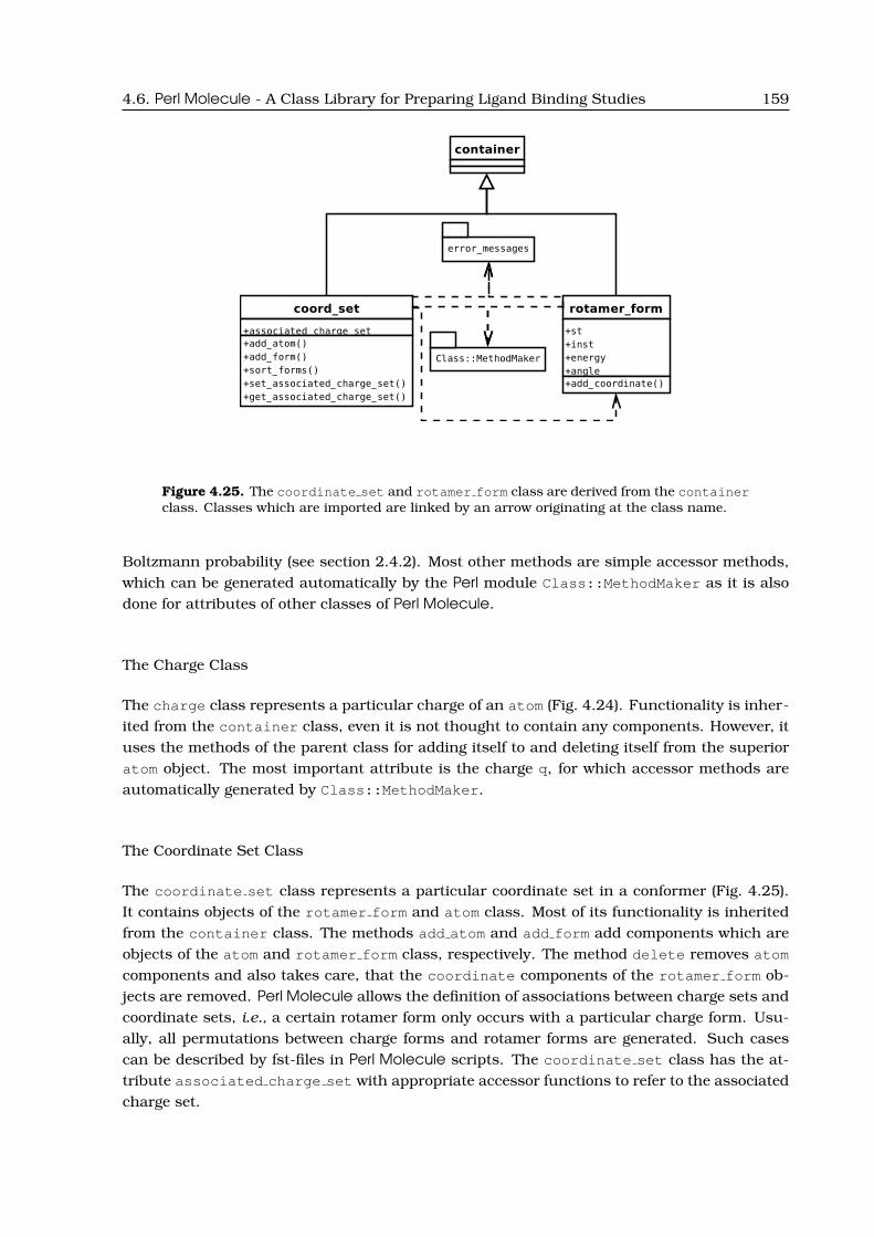
4.6. Perl Molecule - A Class Library for Preparing Ligand Binding Studies 159
Figure 4.25. The coordinate set and rotamer form class are derived from the containerclass. Classes which are imported are linked by an arrow originating at the class name.
Boltzmann probability (see section 2.4.2). Most other methods are simple accessor methods,which can be generated automatically by the Perl module Class::MethodMaker as it is alsodone for attributes of other classes of Perl Molecule.
The Charge Class
The charge class represents a particular charge of an atom (Fig. 4.24). Functionality is inher-ited from the container class, even it is not thought to contain any components. However, ituses the methods of the parent class for adding itself to and deleting itself from the superioratom object. The most important attribute is the charge q, for which accessor methods areautomatically generated by Class::MethodMaker.
The Coordinate Set Class
The coordinate set class represents a particular coordinate set in a conformer (Fig. 4.25).It contains objects of the rotamer form and atom class. Most of its functionality is inheritedfrom the container class. The methods add atom and add form add components which areobjects of the atom and rotamer form class, respectively. The method delete removes atom
components and also takes care, that the coordinate components of the rotamer form ob-jects are removed. Perl Molecule allows the definition of associations between charge sets andcoordinate sets, i.e., a certain rotamer form only occurs with a particular charge form. Usu-ally, all permutations between charge forms and rotamer forms are generated. Such casescan be described by fst-files in Perl Molecule scripts. The coordinate set class has the at-tribute associated charge set with appropriate accessor functions to refer to the associatedcharge set.

160 Development of Software for Ligand Binding Studies
Figure 4.26. The charge set and charge form class are derived from the container class.Classes which are imported are linked by an arrow originating at the class name.
The Rotamer Form Class
The rotamer form class represents a particular rotamer form in a coordinate set (Fig. 4.25).It contains objects of the coordinate class. Most of its functionality is inherited from thecontainer class. The attribute energy contains the rotamer energy of the form. The methodadd coordinate adds objects of the coordinate class as components.
The Charge Set Class
The charge set class represents a particular charge set in a conformer (Fig. 4.26). It containsobjects of the charge form and atom class. Most of its functionality is inherited from thecontainer class. Like the coordinate set class, it has the add atom and add form methodsto add its components. It has the attribute associated coord set and accessor functions torefer to the associated coordinate set.
The Charge Form Class
The charge form class represents a particular charge form in a charge set (Fig. 4.26). Itcontains objects of the charge class. Most of its functionality is inherited from the containerclass. The method setup initializes the two attributes st and inst, which are a reference to ast file, est file, xst file or fst file object and an instance number, respectively. Themethod get is called with a accessor method name of the object stored in st and an instancenumber as parameters. It returns the result of the accessor method call for the instance inst.The method add charge adds objects of the charge class as components.
The Chargegroup Class
The chargegroup class represents a particular charge group in a conformer (Fig. 4.27). It con-tains objects of the chargegroup member class. Most of its functionality is inherited from the

4.6. Perl Molecule - A Class Library for Preparing Ligand Binding Studies 161
Figure 4.27. The chargegroup and chargegroup member class are derived from thecontainer class. Classes which are imported are linked by an arrow originating at theclass name.
container class. The method setup members is called by the method atom::setup charge-
groups. It constructs an object of the chargegroup member class for each atom returnedby the functions topology::get chargegroup or topology::get patch chargegroup. Themethod also initializes the attributes of the new chargegroup member object via the providedaccessor methods. The method add atom associates an atom object with this chargegroup
object by setting the chargegroup variable of the atom object to point to this chargegroup
object. The chargegroup member object, which is the representation of an atom in a charge-
group, is linked with the atom object by calling the set atom method. If the chargegroup
belongs to a site, the atom is set to belong to the same site.
The Chargegroup Member Class
The chargegroup member class represents a particular atom in a chargegroup (Fig. 4.27).Functionality is inherited from the container class, even it is not thought to contain anycomponents. However, it uses the methods of the parent class for adding itself to and deletingitself from the superior chargegroup object. The most important attribute is atom, whichis a reference to the atom object, which is associated with the chargegroup member object.Additionally, each instance contains variables to store information contained about the atomin the topology file, i.e., the charge, the element, the mass and type. The attribute charge
is used to assign charges to atoms read from a pdb-file. The attribute element is used to lookup atom radii based on the chemical element. The other attributes are currently not used.For attributes accessor methods are automatically generated by Class::MethodMaker.
The Site Class
The site class represents a particular site in a conformer. It contains objects of the instanceand atom class (Fig. 4.28). Most of its functionality is inherited from the container and

162 Development of Software for Ligand Binding Studies
Figure 4.28. The site and instance class are derived from the MMcontainer class. Theinstance member class is derived from the container class. Classes which are importedare linked by an arrow originating at the class name.
MMcontainer classes. The add atom method adds the given atom to the site. The methodrecursively also adds all atoms, which are in the same charge group as the atom, makingsure, that a site always has an integer charge. A site can be associated with objects ofthe coordinate set and charge set class to which the atom objects belongs. If all atomobjects only belong to a single set, each instance object can be associated with a particularrotamer form or charge form object. In general, a site may be associated with a set of bothtypes, because different atom objects belong to different charge set and coordinate set
objects. Then, instance objects have to be generated as all permutations of rotamer form
and charge form objects unless the coordinate set and charge set are associated (seeabove). Each permutation can be described by a unique vector in analogy to a state vector ofa microstate. The length of the vector equals the sum of the number of coordinate set andcharge set objects associated with the site. The maximum value at each position of the vectorequals the number of rotamer form or charge form objects of the particular coordinate set
or charge set object represented by the position. All permutations are generated in themethod site::setup using an object of the combinatorics class as helper. For each vec-tor an object of the instance class is created and for each atom component in the site
object an instance member object is created. The instance member object stores a partic-ular combination of coordinate and charge for a single atom. The instance object storesinstance member objects, one for each atom in the site.
The Instance Class
The instance class represents a particular instance in a site. It contains objects of theinstance member class (Fig. 4.28). By that, an instance represents a particular combinationof coordinates and charges for a set of atoms. Most of its functionality is inherited from thecontainer and MMcontainer classes. The methods write and write model write a pqr-filefor the particular instance of a site and for the associated model compound. A number of

4.6. Perl Molecule - A Class Library for Preparing Ligand Binding Studies 163
helper methods are used, which finally call the method atom::write pdb with appropriateparameters. The model compound includes all atoms of the site, all atoms of each residue,which has atoms belonging to the site, and the atoms of charge groups bonded to an atomeither belonging to the site or to an included residue. The method write qmpb writes theQMPB input file section for the instance.
The Instance Member Class
The instance member class represents a particular combination of a coordinate and acharge for a single atom (Fig. 4.28). Functionality is inherited from the container class,even it is not thought to contain any components. However, it uses the methods of the par-ent class for adding itself to and deleting itself from the superior instance object. The mostimportant attributes are a reference each to the associated coordinate and charge object,which are set in the setup method.
Other Classes
Additionally to the classes discussed above, there are other classes, which mostly are objectoriented representation of files. Usually, a file of the appropriate type is parsed and thecontense is provided to other objects by accessor methods. The classes st file, est file,xst file and fst file read the different charge set file formats (Fig. 4.29). The topology
class reads topology files (currently only of CHARMM); the potential class reads files withstored rotamer energies based on torsion potentials; the dunbrack class reads the backbonedependent and backbone independent rotamer database of Dunbrack [101, 102]; the bondi
class reads atom radii from a file (Fig. 4.30) and the charge sites class reads a file containingthe sites, for which different charge forms based on st-files (appendix A.2.1) and est-files(appendix A.2.2) should be applied.
Some classes encapsulate mathematical routines, i.e., the vector class simplifies vector al-gebra, the combinatorics class contains functions to generate state vectors (especially theiterator discussed in section 4.2) and the kabsch class is a SWIG interface (section 4.4.4) tocoordinate superimposition routines by Matthias Ullmann. The kabsch class is used in com-bination with fst-files, ensuring that the atoms bonded to atoms outside the atom set givenin the fst-file are superimposing with minimal root-mean-square deviation. The associatedcoordinate and charge sets in fst-files are usually generated by QM geometry optimizationand charge fitting, which may change the coordinates of the link atoms. It is common, thatthe files are transferred between different crystal structures, where the sites are at differentcoordinate positions.
A third group of classes contain information, which did not fit into any other class. ThePhysCond class encapsulates variables and constants, which reflect the physical conditionsof the calculation. Currently it only contains accessor functions for the absolute temperatureand the gas constant. The module error messages contains some procedures to adjust theverbosity of the output generated by Perl Molecule.

164 Development of Software for Ligand Binding Studies
Figure 4.29. The classes reading different charge set file formats. The files are increasinglycomplex, so that each class can inherit functionality from the classes reading the less com-plex charge set files. Classes which are imported are linked by an arrow originating at theclass name.

4.6. Perl Molecule - A Class Library for Preparing Ligand Binding Studies 165
Figure 4.30. Classes reading different file formats and representing the contense. Classeswhich are imported are linked by an arrow originating at the class name.
4.6.4 Example: Modeling with Perl Molecule
In section 4.6.2 a simple example was given how to replace Multiflex2qmpb by Perl Mole-cule. In section 4.6.3 all the classes of Perl Molecule were discussed in a systematic way.Here, a more complex example is given, which starts with the crystal structure 1CZP [145]of Anabaena ferredoxin as it can be downloaded from the PDB database [127, 128]. Thecrystallographic unit cell contains two molecules (named chain A and chain B), which wererefined independently. The [2Fe-2S] centers are given without chain label in residues FES 599and 699. Since the crystal structure has a very high resolution of 1.17 A, a number of atomsare refined with more than one occupancy. Most interestingly, a peptide bond next to the iron-sulfur center is seen in this (partially) reduced structure in two different orientations (called“CO-in” and “NH-in”) forming an additional hydrogen bond in the NH-in orientation. Sincethis so-called “peptide flip” was not observed in the fully oxidized structure it was assumed,that NH-in structure is characteristic for the reduced form. Results of this study are reportedin section 5.3.
In this script, the structural information contained in the pdb-file is divided into four conform-ers (chain A and B for the two molecules mol-1 and mol-2; occupancy A and B for the peptideorientation CO-in and NH-in, leading to the four structures “mol-1 CO-in”, “mol-1 NH-in”,“mol-2 CO-in” and ”mol-2 NH-in“). The iron-sulfur center, the four ligating cysteins and thebackbone atoms forming the first layer of hydrogen bonds with the iron-sulfur center weregeometry optimized quantum chemically in the oxidized and two reduced forms (reduction ofFe1 and Fe2, respectively). Based on the QM calculations, charges were fitted to the nucleiof the atoms. In the calculation shown here, the charges are stored in xst-files. Alternatively,fst-files can be used analogously including the coordinate changes during the QM geometryoptimization.

166 Development of Software for Ligand Binding Studies
1 #!/ usr/bin/per l −w
2 use s t r i c t ;
3 use error messages ;
4 use molecule3 ;
5 use x s t f i l e ;
6
7 error messages : : set blab ( 2 ) ;
8 #################################
9 # 1CZP
10 #################################
11 my $mol = molecule−>add (undef , ’1CZP ’ ) ;
12 $mol−>read pdb ( ’1CZP.pdb ’ ) ;
The first lines are identical to the example in section 4.6.2. In line 5 the xst file packageis included since it will be needed later. Line 11 creates an empty object of the moleculeclass with the name 1CZP. In the next line it is filled by reading the pdb-file using the methodread pdb. At this point in the previous example the method read pqr was used to read thepqr-file. Currently, the object structure of Perl Molecule contains one molecule with oneconformer and three chains. The pdb-file contains the two molecules with chain labels Aand B. The atoms of the iron-sulfur centers and all crystallographic water molecules have nochain label and are therefore stored in a third chain with label X. The next step is to move theiron-sulfur centers into their respective molecule and delete all remaining water molecules inchain X.
13 # move FES599 from chain X to chain A
14 my $res = $mol−>get residue ( ’FES 599 ’ ) ;
15 my $chain = $mol−>get chain ( ’A ’ ) ;
16 $res−>move( $chain ) ;
17 ## move FES699 from chain X to chain B
18 $res = $mol−>get residue ( ’FES 699 ’ ) ;
19 $chain = $mol−>get chain ( ’B ’ ) ;
20 $res−>move( $chain ) ;
21 # rename FES699 to FES599
22 $res−>set labe l ( ’FES 599 ’ ) ;
23 # delete chain X
24 $chain = $mol−>get chain ( ’X ’ ) ;
25 $chain−>delete ;
Therefore, in line 14 and 18 the method get residue is called for the residues FES 599 andFES 699. It is one of the helper methods provided by the molecule class which does notrequire, that the user of Perl Molecule knows the conformer and chain labels in which theresidues are stored or even the object tree structure underlying Perl Molecule. If the ontologyis extended by adding or removing levels of the taxonomy, scripts using the method will stillwork. Since the molecule class does not contain any residues directly, it recurses throughthe object tree until it reaches objects of the chain class and checks if they contain a residue
object with the given label. If none or more than one object with the given label is found theprogram stops with an error message. On success a reference to the residue is returned. The

4.6. Perl Molecule - A Class Library for Preparing Ligand Binding Studies 167
method get chain used in lines 15 and 19 is analogous to get residue. It recurses untilit finds a chain with the given label and returns a reference to it. In line 16 and 20 themethod move of the residue objects are called with the reference of the destination chain
as parameter. The method move was implemented in the container class and inheritedto all derived classes. The residue object removes itself from its superior chain containerclass by calling member delete and adds itself to the chain class given as parameter by themethod member add. If a member with same label exists in the destination container class(member exists returns TRUE) the method returns FALSE, else it returns a reference to theobject (in the shown script it is not checked for the return value). For consistency in line 22the residue FES 699 of chain B is renamed into FES 599 as the iron-sulfur center is calledin chain A. In line 24 a reference to chain X containing all the water molecules is obtainedand in line 25 the chain is deleted. The method delete (also provided by the container
class) removes the object by recursively deleting all objects it contains. In the next step, themolecule in chain with label B is moved into a separate conformer with label ”mol-2 CO-in“.
26 # move chain B into new conformer
27 my $conf = conformer−>add ($mol , ’mol−2 CO−in ’ ) ;
28 $chain = $mol−>get chain ( ’B ’ ) ;
29 $chain−>move( $conf ) ;
30 # rename chain B to chain A
31 $chain−>set labe l ( ’A ’ ) ;
Therefore, in line 27 a new empty conformer object is created with the label ”mol-2 CO-in“and the molecule as container class. In line 28 again the get chain method is used to obtaina reference to the chain object with label B (mol-2) and move it into the new conformer (line29). Here the same move method of the container class is used as it was used before tomove residues. The only chain in conformer ”mol-2 CO-in“ should carry the label A, which ischanged using the set label method (line 31).
In the following a CHARMM topology file should be read and used to define charge groupsand the molecular topology graph. The topology file uses the CTER patch, which calls theC-terminal carboxyl oxygens OT1 and OT2.
32 # set O and OXT to OT1 and OT2
33 $mol−>rename atom ( ’A ’ , ’TYR 98 ’ , ’O ’ , ’OT1 ’ ) ;
34 $mol−>rename atom ( ’A ’ , ’TYR 98 ’ , ’OXT ’ , ’OT2 ’ ) ;
35 # set a l l HIS to HSP
36 $mol−>rename residue ( ’A ’ , ’HIS ’ , ’HSP ’ ) ;
Therefore, the atoms O and OXT are renamed in both conformers using the method rename -
atom. The method takes the chain label, residue label and the old and new atom name asparameters. Internally it recurses through the object structure and calls rename for eachobject of type atom. The rename method of the atom class returns immediately if the chain,residue or old atom label do not match, else it uses the set label method to set the newatom label. The CHARMM topology file contains a residue HSP, which is a doubly protonatedhistidine. Since the hydrogen placement procedure in the following has to place both the ε-and δ-proton, all histidine residues have to be named HSP. The method rename residue inline 36 is analogous to rename atom in recursing through the object tree and renaming allresidues, which match the given parameters.

168 Development of Software for Ligand Binding Studies
The hydrogen adding procedure will add rotateable hydrogen (e.g., in hydroxyl groups) asmany times as there are hydrogen bond acceptors in the vicinity (according to geometriccriteria). To assign energies for the different rotamers, potential energies were calculated andstored as function of the torsion angle. The method setup rotamer sites (line 37) reads a filecharmm.potentials (see appendix A.4.3), which contains the residue names and four atomsdefining the dihedral angle of the torsion together with a file name, in which the pre-computedtorsion angles and energies are stored. Those files are read and stored into potential objects.
37 $mol−>setup rotamer sites ( ’charmm. potentials ’ ) ;
38 my %topology = (
39 method => ’ topology ’ ,
40 fo rce f i e ld => ’charmm ’ ,
41 f i l e => [
42 ’ top all27 prot na . r t f ’ ,
43 ’ fes . r t f ’
44 ] ,
45 patch => [
46 ’NTER 1 ’ ,
47 ’CTER 98 ’ ,
48 ]
49 ) ;
50 $mol−>setup charge groups(\%topology ) ;
51 $mol−>setup graph(\%topology ) ;
52 $mol−>setup rotamers ;
53 $mol−>setup sites ;
The lines 38 to 51 are analogous to the simpler example. An object of the topology classis generated and used to define charge groups (via chargegroup and chargegroup member
objects). The topology object is also used to construct the graph of bonded atoms to definethe topology of the molecule. In line 52 the method setup rotamers is called, which con-structs coordinate set and rotamer form objects by calling setup rotamers for each atom(described in detail in the section about the atom class). At this point only rotamer form
objects are created for the sidechains with different occupancies and for the backbone sec-tion including the peptide flip. Energies of the rotamers are calculated from the occupancyvalues interpreted as probabilities. The method molecule::setup sites calls the methodatom::setup sites for each atom object. The method atom::setup sites constructs a site
object and generates instance and instance member objects via calling the site::setup
method. (Also these methods were described in more detail before.)
In the next step, the two rotamer forms for the peptide flip (CO-in and NH-in) should beseparated into conformers. Since two conformers are already present (from mol-1 and mol-2), this leads to four conformers (”mol-1 CO-in“, ”mol-1 NH-in“, ”mol-2 CO-in“ and ”mol-2NH-in“).
54 # coordinate set N ALA 45 A is peptide f l i p , I separate the two rotamer forms
55 # into two conformers
56 # conf 0 ( id : 0) −> mol−1 CO−in ( coordinate set N ALA 45 A only
57 # rotamer form A 1CZP .pdb )
58 # −> mol−1 NH−in ( coordinate set N ALA 45 A only

4.6. Perl Molecule - A Class Library for Preparing Ligand Binding Studies 169
59 # rotamer form B 1CZP .pdb )
60 # conf mol−2 CO−in ( id : 1) −> mol−2 CO−in ( coordinate set N ALA 45 A only
61 # rotamer form A 1CZP .pdb )
62 # −> mol−2 NH−in ( coordinate set N ALA 45 A only
63 # rotamer form B 1CZP .pdb )
64 $conf = $mol−>copy conformer (0 , ’mol−1 NH−in ’ ) ;
65 $conf−>delete rotamer form ( ’N ALA 45 A ’ , ’A 1CZP.pdb ’ ) ;
66 $conf = $mol−>get re f by type id (0 , ’ conformer ’ ) ;
67 $conf−> delete rotamer form ( ’N ALA 45 A ’ , ’B 1CZP.pdb ’ ) ;
68 $conf = $mol−>copy conformer (1 , ’mol−2 NH−in ’ ) ;
69 $conf−>delete rotamer form ( ’N ALA 45 A ’ , ’A 1CZP.pdb ’ ) ;
70 $conf = $mol−>get re f by type id (1 , ’ conformer ’ ) ;
71 $conf−>delete rotamer form ( ’N ALA 45 A ’ , ’B 1CZP.pdb ’ ) ;
72 $mol−>get member ( ’0 ’ )−>set labe l ( ’mol−1 CO−in ’ ) ;
The method copy conformer copies in line 64 the first conformer (mol-1, index 0) into anew conformer (with label ”mol-1 NH-in“) within the same molecule. From conformer ”mol-1 NH-in“ the rotamer form CO-in with label A 1CZP.pdb of the coordinate set with labelN ALA 45 A is deleted (delete rotamer form in line 65). In line 66 a reference to the con-former with index 0 is obtained and used in line 67 to delete the rotamer form NH-in withlabel B 1CZP.pdb. The conformer with index 1 (and label ”mol-2 CO-in“, line 27) is processedanalogously. Finally, in line 72 the label for conformer 0 (default, since no label is given inthe pdb-file) is changed to ”mol-1 CO-in“. As result, the molecule object has four conformers,where ”mol-1 CO-in“ and ”mol-1 NH-in“ originate from chain A (mol-1) and ”mol-2 CO-in“ and”mol-2 NH-in“ originate from chain B (mol-2). ”mol-1 CO-in“ and ”mol-2 CO-in“ contain thepeptide flip in the orientation CO-in, which had the occupancy label A. ”mol-1 NH-in“ and”mol-2 NH-in“ contain the peptide flip in the orientation NH-in, which had the occupancylabel B.
The next step is to add hydrogens using the external program Hwire.
73 # mult iple hydrogens as occupancies/s i tes
74 my %param = (
75 method => ’ instance x ’ ,
76 program => ’ hwire ’ ,
77 binary => ’ /home/essigke/bin/hwire −f ’ ,
78 hwire parameter => {
79 par => [
80 ’charmm22 hpath. dat ’ ,
81 ’ fes . dat ’
82 ] ,
83 d1max => ’ 3.8 ’ ,
84 d2max => ’ 4.5 ’ ,
85 alpha => ’110 ’ ,
86 epsilon => ’60 ’ ,
87 zeta => ’60 ’ ,
88 hydrogens => ’ on ’ ,
89 rotamers => ’ on ’ ,
90 lonepairs => ’ o f f ’ ,

170 Development of Software for Ligand Binding Studies
91 patch => [
92 ’NTER 1 A ’ ,
93 ’CYS FE1 41 A ’ ,
94 ’CYS FE1 46 A ’ ,
95 ’CYS FE2 49 A ’ ,
96 ’CYS FE2 79 A ’
97 ]
98 } ,
99 ) ;
100 $mol−>add hydrogen(\%param ) ;
101 $mol−>setup charge groups(\%topology ) ;
102 $mol−>setup graph(\%topology ) ;
103 $mol−>setup rotamers ;
104 $mol−>setup sites ;
In lines 74 to 99 a hash is filled, which can be passed to the method add hydrogen in line100, which performs the addition of hydrogens. Since there are so many programs availablefor this purpose, all with their strength and weaknesses, I assumed that it would be usefullto have this part of Perl Molecule variable by a plug-in infrastructure (similar to the potentialusage of different topology file formats). Currently, only Hwire is available, which was dis-cussed with some of its parameters in section 2.4.3. A problem of Hwire is, that it can not dealproperly with rotamers as they originate here from sidechains with multiple occupancies. Theadd hydrogen method therefore generates separate conformers, lets Hwire add hydrogens toeach of them and finally joins the conformers to retrieve the rotamers with hydrogens added.The generation of conformers from rotamers requires to deal with the different combinationsof rotamers in a structure. Internally, add hydrogen uses the combinatorics class, whichprovides different methods of generating state vectors. Usually one wants to use the methodcombinatorics::full x, which generates a complete set of state vectors. For example, astructure with rotamers in five coordinate set objects and three rotamer form objects each,would lead to 35 = 243 conformations to which hydrogens have to be added (or 972 for the fourconformations of 1CZP). For such a large number of structures, hydrogen adding would bevery time consuming. The method combinatorics::instance x generates a structure foreach instance (or rotamer form in this case), leading to three conformers in the previous ex-ample (with state vectors (00000), (11111) and (22222)). The method combinatorics::site x
generates a structure for each site (coordinate set) in each instance rotamer form, while allother sites are in their reference instance. In the example, it would lead to eleven structures((3−1) ·5+1 = 11, with state vectors of e.g., (00000), (10000), (20000), (01000), (02000) . . . ). For the1CZP structure, it was found that the instance x method is sufficient, since the sidechainswith different occupancies are well separated on the surface of the protein. However, for otherstructures this method may not be sufficient. Probably the best way to determine whichmethod to use, if it can not be decided by quick visual inspection, is to try the different meth-ods in a test calculations. If the methods including more conformers do not increase thenumber of hydrogen positions for rotateable hydrogen, the cheaper method is sufficient. Usu-ally, Hwire will place rotateable hydrogens in slightly different positions, which complicatesthis analysis. To remove these artefacts, the method molecule::remove close rotamers isprovided, which takes a threshold dihedral angle as parameter. All rotamer forms and associ-

4.6. Perl Molecule - A Class Library for Preparing Ligand Binding Studies 171
ated hydrogen coordinates are deleted, which are closer than the threshold dihedral angle toan accepted rotamer form.
After adding hydrogen, the new atoms have to be assigned to the present charge groups andthe molecular topology has to be updated to include the bonds to the hydrogen (line 101 and102). New coordinate sets are created due to hydrogen rotamers or existing coordinate setsget more rotamer forms due to a combination of, e.g., sidechain occupancies and hydrogenrotamers. Therefore setup rotamers is called again (line 103). Since the coordinate set
and rotamer form objects changed, the site, instance and instance member objects haveto be adjusted by setup sites (line 104).
The pdb-file does not contain any information on the atom radii, unlike the pqr-file in theprevious example. Therefore, the radii are assigned from a file. Also different charge formshave to be assigned to protonateable groups of the protein and the reduction forms of theiron-sulfur center.
105 # setup bondi ( assign radi i to atoms )
106 %param = (
107 method => ’ bondi ’ ,
108 f i l e => ’ bondi . rad ’
109 ) ;
110 $mol−>add radii (\%param ) ;
111 #
112 # assign addit ional charges from . st /. est f i l e s , include as instances
113 # assign energies for instances based on model pK or ADF energy
114 #
115 $mol−>setup charge sites ( ’ vFdx . s i tes ’ ) ;
116 #
117 # setup xst − est f i l e s containing mult iple residues from mult iple chains
118 foreach my $conf label (qw( ’mol−1 CO−in ’ ’mol−1 NH−in ’ ’mol−2 CO−in ’ ’mol−2 NH−in ’ ) ) {
119 my $xst name = ”1CZP ” . $conf label . ” . xst ” ;
120 my $xst = xs t f i l e3−>new( $xst name ) ;
121 my $conf = $mol−>get member ( $conf label ) ;
122 $xst−>setup ( $conf ) ;
123 }
124 $mol−>setup sites ;
The method add radii in line 110 takes also a hash as parameter. The hash (line 106 to109) contains analogously to the topology hash a key method and a key file. The method
allows extensions for other methods or file formats to determine radii (e.g., from some forcefield, PARSE radii [146], van-der-Waals radii etc.). Currently only a single file format used forBondi [147] radii is available (appendix A.5.4). In line 115 the method setup charge sites
is used to define charge set and charge form objects as in the previous example. By thismethod only charge sets can be defined, which are not larger than one residue, because thesites file is residue based. Future versions may change the sites file to allow also to specify xst-files and fst-files. A different xst-file should be used for each of the four conformers. It is donein this example (line 118 to 123) by iterating over the conformer labels, constructing a xst-filename, reading the file by constructing a xst object and passing a conformer object (selectedby the label) to the xst::setup method. In line 124 the method setup sites is called to
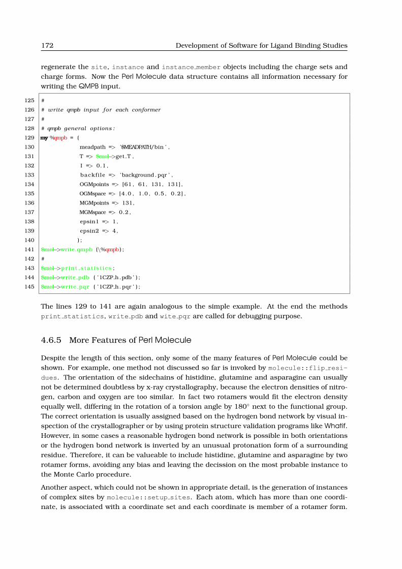
172 Development of Software for Ligand Binding Studies
regenerate the site, instance and instance member objects including the charge sets andcharge forms. Now the Perl Molecule data structure contains all information necessary forwriting the QMPB input.
125 #
126 # write qmpb input for each conformer
127 #
128 # qmpb general options :
129 my %qmpb = (
130 meadpath => ’$MEADPATH/bin ’ ,
131 T => $mol−>get T ,
132 I => 0.1 ,
133 backfi le => ’ background . pqr ’ ,
134 OGMpoints => [61 , 61, 131, 131] ,
135 OGMspace => [4.0 , 1.0 , 0.5 , 0.2] ,
136 MGMpoints => 131,
137 MGMspace => 0.2 ,
138 epsin1 => 1,
139 epsin2 => 4,
140 ) ;
141 $mol−>write qmpb (\%qmpb) ;
142 #
143 $mol−>pr in t s ta t i s t i c s ;
144 $mol−>write pdb ( ’1CZP h.pdb ’ ) ;
145 $mol−>write pqr ( ’1CZP h. pqr ’ ) ;
The lines 129 to 141 are again analogous to the simple example. At the end the methodsprint statistics, write pdb and wite pqr are called for debugging purpose.
4.6.5 More Features of Perl Molecule
Despite the length of this section, only some of the many features of Perl Molecule could beshown. For example, one method not discussed so far is invoked by molecule::flip resi-
dues. The orientation of the sidechains of histidine, glutamine and asparagine can usuallynot be determined doubtless by x-ray crystallography, because the electron densities of nitro-gen, carbon and oxygen are too similar. In fact two rotamers would fit the electron densityequally well, differing in the rotation of a torsion angle by 180◦ next to the functional group.The correct orientation is usually assigned based on the hydrogen bond network by visual in-spection of the crystallographer or by using protein structure validation programs like Whatif.However, in some cases a reasonable hydrogen bond network is possible in both orientationsor the hydrogen bond network is inverted by an unusual protonation form of a surroundingresidue. Therefore, it can be valueable to include histidine, glutamine and asparagine by tworotamer forms, avoiding any bias and leaving the decission on the most probable instance tothe Monte Carlo procedure.
Another aspect, which could not be shown in appropriate detail, is the generation of instancesof complex sites by molecule::setup sites. Each atom, which has more than one coordi-nate, is associated with a coordinate set and each coordinate is member of a rotamer form.

4.7. Summary 173
Bonded atoms with more than one coordinate are assigned to the same coordinate set, e.g.,using the occupancy information given in a pdb-file. Charge sets are usually defined by one ofthe charge set file types (st-file, est-file, xst-file or fst-file). Upon generation of sites, coordinatesets and charge sets are combined. It is possible that a charge set contains atoms of differentcoordinate sets and a coordinate set contains atoms of different charge sets. Since sites haveto have an integer charge, not only the atoms belonging to coordinate sets and charge setsare included, but all atoms belonging to the same charge group as any atom of one of thesets. It is possible, that the atoms, which were included due to charge groups also belong toadditional coordinate sets or charge sets, which need to be added to the site. The method actsaccording to these rules until a consistent set of atoms for the site can be found. Then, allcoordinate sets and charge sets are combined by generating instances for all permutations ofrotamer forms and charge forms. Therefore, sites constructed from many coordinate sets andcharge sets can have very many instances. Without assistance by the program, it would bevery hard for a human to make the right choice of atoms to ensure that all rules are fulfilledand that all permutations of coordinates and charges are included in the subsequent QMPBcalculations.
The feature to generate sidechain rotamers based on a rotamer database, is also not shownin one of the examples, but it will be discussed in section 5.3.3. More capabilities shouldbe relatively easy to add to Perl Molecule because of the detailed class hierarchy and thechemical and physical knowledge already implemented. Needs of future projects will drive thedevelopment on Perl Molecule.
4.7 Summary
To make the theory developed in the previous chapter applicable for larger biomolecules, aset of programs was developed. QMPB is the program to compute intrinsic energies and inter-action energies. The intrinsic energy contains contributions, which can be obtained experi-mentally, by molecular mechanical or quantum chemical calculations and have to be given asinput to QMPB. Furthermore, pqr-files are required for each instance specifying coordinatesand charges for each atom of the site. QMPB interprets its input file to set up continuumelectrostatic calculations to compute transfer energies. A LPBE solver is not implemented inQMPB, but the program uses a set of external programs to perform the calculations. Thisapproach has the advantage, that on one hand, the PB solver can be easily exchanged byreplacing the programs, on the other hand parallelization of the time consuming step solvingthe LPBE, does not need to be done within QMPB. Instead, QMPB writes a shell script, whichcan be executed directly and performs the calls to the PB solver sequentially. Alternatively,a additional program is used splitting the shell script into program calls to be executed ondifferent computers. The program can also use an existing queuing system to distribute theworkload on a compute cluster. Therefore it is easily possible to optimize the program forthe local computing environment without modifying QMPB directly. In a second run, QMPBcollects the output of the helper programs, calculates the intrinsic energies and interactionenergies and writes them into suitable files for further processing.
During development of QMPB, it was an aim to keep the program as transparent as possible.Splitting the calculation in several steps with extensive input and output files and making

174 Development of Software for Ligand Binding Studies
the electrostatic calculations repeatable without recomputing the rest of the systems allowsthe user to follow every step. This transparency is valueable teaching students and simplifiesextensions to the program as the progress of research requires them.
For small systems the output of QMPB can be used to solve the grand canonical partitionfunction, e.g., by the program SMT. For larger systems, the probability of instances can beapproximated, e.g., by the Monte Carlo program GMCT. In practice, probabilities of instancesat a fixed set of chemical potentials are not of as much interest as the titration behavior of asite, when changeing the chemical potentials. Therefore, each chemical potential is scannedin small steps over a wide range, which in most cases is computationally more demandingthan solving the LPBE. In fact, QMPB scales linearly with the number of instances, while theMonte Carlo algorithm has an exponential scaling behavior with the number of ligand types,i.e., dimensions in which the chemical potential needs to be varied. Since for many biologicalquestions studies with many ligand types are of great interest and the generalized titrationtheory and QMPB do not impose limits in this respect anymore, future applications will cer-tainly require such high-dimensional titration calculations. The adaptive mesh refinementalgorithm (AMR) is an approach to reduce the computational cost. The basic idea is to ex-clude instances, which do not titrate in a region of chemical potential space on a coarse gridfor calculations on finer grids. This reduces the number of points, at which probabilities needto be calculated and reduces the state vector length for analytical or Monte Carlo calculationsfor the remaining sites.
QMPB relies on a large number of input files, which can be complex for certain sites. Manualgeneration of these input files is tedious and error prone. Shell scripts written for this purposesuffer from readability, reliability and reueseability. One source of these problems is thelack of complex data structures in shell script, another the inherent complexity to process abiomolecular structure to generate input for electrostatic calculations. A significant amountof chemical and physical knowledge is required to set up the calculations in a meaningfulway, e.g., knowledge of the topology of the molecule is required to choose the right atoms forsites. Since all instances of a site should have an integer charge, charge groups - known fromforce fields - are a helpful concept to group atoms. Sites may be complex containing severalsets of atoms changing their coordinates in a concerted way (rotamer forms of a coordinateset) and sets of atoms changeing their charge (charge forms of a charge set). All permutationsof rotamer forms and charge forms need to be generated as instances. To ease these andother tasks, the class library Perl Molecule was written. It implements an ontology following acommon hierarchical view on biomolecules. By reading topological descriptions of moleculesand other parameter files, sufficient information is gathered to guide the user through theprocess of input preparation. However, it was felt too inflexible to write a single program forthis purpose, because biomolecules are too complex to cover all cases. Future developmentsor just different opinions of different users are likely to change the protocol. Therefore PerlMolecule is a class library, which allows the user to write powerful Perl scripts with littleeffort, but sufficient flexibility for a large variety of use cases.

CHAPTER 5
EXAMPLES FOR LIGAND BINDING STUDIES
5.1 Lysozyme as Test Case for QMPB
The use of hen egg white lysozyme (HEWL) as test case for protein electrostatics has a longhistory [27, 32, 33, 35, 46, 48–52]. HEWL is a small enzyme of 129 residue length and 21titrateable residues (1 histidine, 2 glutamate, 7 aspartate, 3 tyrosine and 7 lysine, C-terminalleucine). Most titrateable residues are solvent exposed and their pKa values were experi-mentally determined. Therefore, the protein was often used as benchmark system, assumingthat a low RMSD between the calculated and experimental pKa values is a good measure forthe quality of a method in predicting pKa values. However, the studies have shown, thatrather simple methods using a high dielectric constant for the protein (20 and higher [48, 50])give lower RMSD values than physically more sophisticated methods using lower dielectricconstants [32]. In contrast, the buried active site residues can be predicted better with lowdielectric constants and a physically better model. The reason is that for a small protein mosttitrateable residues are on the surface and are very flexible. This flexibility is hard to ac-count for by continuum electrostatics, especially if crystal structures are used showing onlya single rotamer. Implicitly a higher dielectric constant accounts for this flexibility and re-duces the RMSD. Nevertheless, little can be learned from such a model, because usually themost important residues are buried at least partially and have to be in a specific orientation.Georgescu et al. [33] have shown, that as good RMSD pKa values can be achieved with adielectric constant of 4, if sidechain rotamers generated by a rotamer database were takeninto account. In their calculation the RMSD gets worse for higher dielectric constants as onewould expect for a model taking flexibility into account.
Donald Bashford, the author of the MEAD package, used HEWL as test enzyme for his programMultiflex. He provides the input data for his early work [35] and scripts to run his programsand to reproduce his results. I provide the same example as test case for Multiflex2qmpb andQMPB to compare to Multiflex.
Fig. 5.1 shows that the titration curves obtained with Multiflex and Karlsberg [34] are identicalwith those obtained with Multiflex2qmpb, QMPB and GMCT within sampling errors of theMonte Carlo procedure. Therefore, the new programs can replace the old programs, but addadditional functionality, which is demonstrated in the following example applications.
175

176 Examples for Ligand Binding Studies
0 2 4 6 8 10 12 14pH
0
0.2
0.4
0.6
0.8
1<
x>
Figure 5.1. Titration curves of titrateable residues in lysozyme calculated with the old setof programs Multiflex and Karlsberg (black) as well as calculated with the new set of programsMultiflex2qmpb, QMPB and GMCT (red). The curves are identical within the sampling errorof the Monte Carlo procedures.
5.2 Effects of Serine Phosphorylation and Histidine Protonation
and Phosphorylation on HPr
This project was done in collaboration with Nadine Homeyer, Heike Meiselbach and HeinrichSticht (University of Erlangen). The results are published [148, 149].
In both publications, the molecular dynamics simulations and most of the structural analysiswere performed by Nadine Homeyer in the group of Heinrich Sticht, while the protonationprobability calculations (using QMPB) and the calculations using the microstate model weredone by me. Matthias Ullmann contributed by helpful suggestions, discussion and formula-tion of the manuscripts.
5.2.1 The Biological Role of HPr
The histidine-containing phosphocarrier protein (HPr) is involved in the regulation of a num-ber of processes associated with carbohydrate uptake and consumption in various bacterialspecies. It plays a central role in the phosphoenolpyruvate:sugar phosphotransferase system
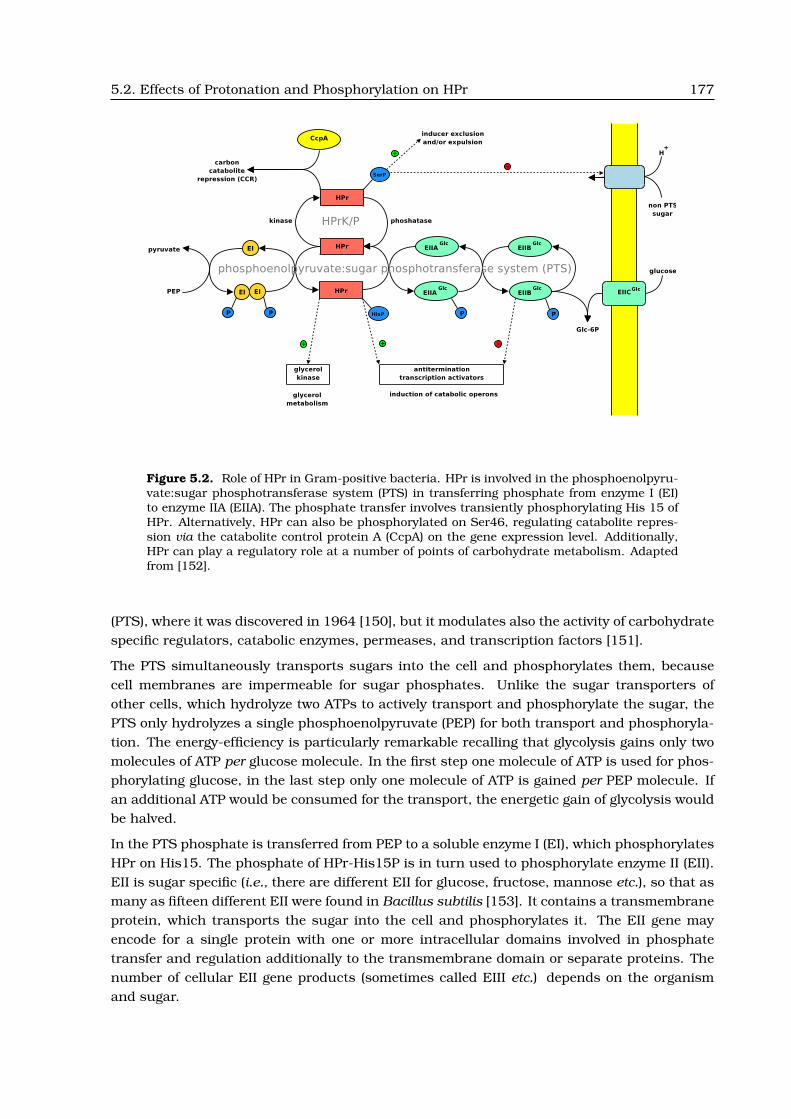
5.2. Effects of Protonation and Phosphorylation on HPr 177
Figure 5.2. Role of HPr in Gram-positive bacteria. HPr is involved in the phosphoenolpyru-vate:sugar phosphotransferase system (PTS) in transferring phosphate from enzyme I (EI)to enzyme IIA (EIIA). The phosphate transfer involves transiently phosphorylating His 15 ofHPr. Alternatively, HPr can also be phosphorylated on Ser46, regulating catabolite repres-sion via the catabolite control protein A (CcpA) on the gene expression level. Additionally,HPr can play a regulatory role at a number of points of carbohydrate metabolism. Adaptedfrom [152].
(PTS), where it was discovered in 1964 [150], but it modulates also the activity of carbohydratespecific regulators, catabolic enzymes, permeases, and transcription factors [151].
The PTS simultaneously transports sugars into the cell and phosphorylates them, becausecell membranes are impermeable for sugar phosphates. Unlike the sugar transporters ofother cells, which hydrolyze two ATPs to actively transport and phosphorylate the sugar, thePTS only hydrolyzes a single phosphoenolpyruvate (PEP) for both transport and phosphoryla-tion. The energy-efficiency is particularly remarkable recalling that glycolysis gains only twomolecules of ATP per glucose molecule. In the first step one molecule of ATP is used for phos-phorylating glucose, in the last step only one molecule of ATP is gained per PEP molecule. Ifan additional ATP would be consumed for the transport, the energetic gain of glycolysis wouldbe halved.
In the PTS phosphate is transferred from PEP to a soluble enzyme I (EI), which phosphorylatesHPr on His15. The phosphate of HPr-His15P is in turn used to phosphorylate enzyme II (EII).EII is sugar specific (i.e., there are different EII for glucose, fructose, mannose etc.), so that asmany as fifteen different EII were found in Bacillus subtilis [153]. It contains a transmembraneprotein, which transports the sugar into the cell and phosphorylates it. The EII gene mayencode for a single protein with one or more intracellular domains involved in phosphatetransfer and regulation additionally to the transmembrane domain or separate proteins. Thenumber of cellular EII gene products (sometimes called EIII etc.) depends on the organismand sugar.

178 Examples for Ligand Binding Studies
In Gram-negative bacteria the PTS regulation is particularly well studied for the glucose trans-port of Escherichia coli [154]. Here, phosphorylated EIIAGlc activates adenylate cyclase, whichproduces cAMP as a ligand for the catabolite gene activator protein. It enhances transcrip-tion of catabolic genes in the absence of glucose. Dephosphorylated EIIAGlc, occurring in thepresence of glucose, inhibits the influx of lactose into the bacterium and thus prevents theinduction of the lac operon.
In Gram-positive bacteria, carbon catabolite repression (CCR) operates by phosphorylation ofHPr at Ser46 by the ATP dependent kinase/phosphatase HPrK/P [155–158]. At high levelsof ATP as in glycolysing bacteria, the kinase activity of HPrK/P is dominant, producing HPr-Ser46P, which is only slowly phosphorylated by EI. Therefore, the PTS is down-regulated dueto a depletion of unphosphorylated HPr. At low levels of ATP, the phosphatase activity ofHPrK/P becomes dominant, dephosphorylating HPr and therefore up-regulating the PTS.
Additionally to this direct regulation of the PTS, HPr-Ser46P binds to the transcriptional reg-ulator catabolite control protein A (CcpA) to convert it into its DNA-binding-competent confor-mation. CcpA binds to operator-like catabolite responsive element (cre) sequences, which arecommon motifs in front of many operons involved in carbohydrate degradation. Experimentaldata indicate, that the expression of 8% of all B. subtilis genes is regulated by CcpA [159, 160].Thus, HPr-Ser46P is directly involved in regulation of gene expression.
Also HPr-His15P is involved in regulation. The antiterminator proteins of the bgl-sac familyare regulated by phosphorylation at conserved histidine residues in the PTS regulatory do-mains (PRDs). Transcription of several operons involved in carbohydrate utilization appearsto be controlled by this mechanism. HPr was also shown to allosterically stimulate glycogenphosphatase in E. coli. In Gram-positive bacteria, glycerol kinase is activated by phosphory-lation at a histidine by HPr-His15P coordinating glycerol utilization with utilization of othercarbon sources [161].
HPr is an α-β protein. The core is formed by a four-stranded, antiparallel β-sheet, which isconnected by two long helices (α1, α3) and one short helix (α2). The two phosporylation sitesof His15 and Ser46 are shown in Fig. 5.3.
The aim of the project was to study the structure, dynamics and physicochemical propertiesof Ser46 phosphorylation and His15 protonation and phosphorylation to draw conclusionshow HPr performs its regulatory functions.
5.2.2 Phosphorylation of Ser46
The first part of the study analyzed HPr-Ser46P in solution and its complex formation withCcpA [148]. The major part of the work was performed by Nadine Homeyer in the group ofHeinrich Sticht, who did structural studies, MD simulations, and in silico alanine scanning.Their results are summarized here only in brief. An important question within this project,however, was the protonation state of the phosphate bound to HPr, which I calculated bycontinuum electrostatics using my program QMPB.
Until now, there is no experimentally determined pKa value for HPr to compare the resultsdirectly. However, studies on model peptides containing phosphoserine gave a pKa value of5.96 [163]. Since due to the protein environment, the pKa value might shift significantly, it

5.2. Effects of Protonation and Phosphorylation on HPr 179
His15Arg17
Ser46NT
CT
Figure 5.3. Structure of HPr. The backbone is colored by a gradient from N-terminus (red)to the C-terminus (blue). Important residues are shown. The figure was prepared with VMDbased on the crystal structure 1PTF [162].
could not be ruled out a priori, that the phosphate group could also be singly protonated atneutral pH.
MD simulations were done staring from models 1 and 16 of the NMR structure 1JEM [164].Therefore, the phosphorylation on His15 was removed and modeled onto Ser46. The phos-phate was assumed to be doubly negative charged, unprotonated or singly negative charged,singly protonated. During the MD simulation it was observed, that the sidechain of Asn43and the phosphate oxygens are frequently within hydrogen bonding distance (48% and 66% ofthe time for 1JEM - 1 and 1JEM - 16, respectively, using a donor-acceptor distance of smallerthan 2.2 A and an O · · ·H − N angle larger than 150◦ as hydrogen bond criteria). In the al-ternative, non-hydrogen-bonded conformation Ser46P was observed in an orientation, wherethe phosphate group is pointing towards the solvent and does not form any intramolecularinteractions. We assumed, that the hydrogen bond may have an influence on the apparentpKa value of the phosphate group. Therefore, I performed calculations of the apparent pKa
value with and without hydrogen bond present from snapshots of the MD trajectories startedassuming full deprotonation or single protonation of the phosphate. The results are shown inTab. 5.1.
It is evident, that my results of the protonation probability calculations depend to a significantdegree on the input structure. Calculations based on structures taken from the trajectorywhere protonation was assumed, led to results with increased protonation probability, i.e.,a higher apparent pKa value. If the hydrogen bond with Asn43 is present, the deprotonatedform is stabilized, leading to lower apparent pKa values. Such a biasing of pKa calculations

180 Examples for Ligand Binding Studies
Structure - hydrogen-bonded non-hydrogen-bonded
Model MD time (ps) pKa MD time (ps) pKa
doubly deprotonated Ser46P in MD trajectory
1JEM - 1 1000 5.4 1500 6.2
4000 5.7 5500 6.2
1JEM - 16 2000 5.9 2800 6.1
3500 6.0 5000 5.9
singly protonated Ser46P MD trajectory
1JEM - 1 2300 6.0 500 6.8
2800 6.2 1000 6.8
1JEM - 16 1600 6.6 500 6.6
2300 6.0 1000 6.3
Table 5.1. Calculated apparent pKa values of HPr-Ser46P. The structures are snapshots ofMD simulations started assuming a doubly deprotonated and singly protonated phosphate,respectively. The snaphosts were chosen to have a hydrogen bond between Asn43 (HD22)and one of the phosphate oxygens present or not.
by MD simulation was observed by others before [165]. Nevertheless, this bias is such small,that the calculated pKa value varies in less than one unit from the value for the model peptide.Assuming, that the snapshots are representative for the ensemble, one can conclude that thedoubly deprotonated form is predominant at neutral pH.
Analysis of the sequence of HPr proteins revealed, that the asparagine forming the hydrogenbond during the MD simulation is strictly conserved within the Gram-positive bacteria thatpossess HPrK/P and CcpA, but no conserved residue is present in Gram-negative bacteria.Therefore, it was assumed, that Asn43 plays an important role in CCR via Ser46 phosphory-lation. Structural analysis and MD simulations of the interaction of HPr-Ser46P with CcpAindicated, that Asn43 might be important for fixation of the phosphate group in a conforma-tion consistent with binding. Thus, the form with hydrogen bond is the binding-competentform. In the bound form, however the hydrogen bond between phosphate group and Asn43is not present, but the intramolecular hydrogen bond is replaced by intermolecular interac-tions. The role of several residues in the binding interface between the proteins were studiedby alanine scanning giving insight into the discrimination of CcpA between different phospho-rylation states at His15 and Ser46 of HPr.
5.2.3 Protonation of His15
The second part of the study [149] investigated the protonation and conformational changeof His15 in HPr. Unphoshorylated His15 was found in two conformations, a CLOSED confor-

5.2. Effects of Protonation and Phosphorylation on HPr 181
mation, where His15(Nδ1) is in short distance to Arg17(N) and an OPEN conformation, wherethe histidine sidechain points into the solvent. The structures obtained with the OPEN con-formation were determined at low pH (1FU0 at pH 4.2 [152] and 1PTF at pH 5.0 [162]), whilethe CLOSED conformations were found in structures around pH 7 [164, 166–171]. However,it was unclear, if the conformational change of His15 is correlated with a protonation of theimidazole ring.
I performed protonation probability calculations on OPEN and CLOSED structures separatelybased on different crystal and NMR structures. The CLOSED structures are primarily proto-nated on Nε2 in the singly-protonated form and have an apparent pKa value of about 4. TheOPEN structures are primarily protonated on Nδ1 in the singly-protonated form and have anapparent pKa value of below 7 (Tab. 5.2). We aimed to decompose the apparent pKa value ofHis15 into Born, background and interaction energy (as discussed in section 3.2). However,the interaction energy is a tensor containing the interaction of a particular instance of a site(here His15), with all other instances of all other sites. Instead, for the energy decomposi-tion, a single energy is required, which represents the mean-field according to the probability〈xi(lm, {µλ})〉 of the instances m of other sites l in conformer i at a particular set of ther-modynamic variables {µλ}. I formulated a mean-field interaction energy 〈Ginter,i(jk, {µλ})〉 forinstance k of site j (here His15) as:
〈Ginter,i(jk, {µλ})〉 =Nsite,i∑l 6=j
Ninstance,i,l∑m
Ginter,i(jk, lm)〈xi(lm, {µλ})〉 (5.1)
This formulation is similar to the Tanford-Roxby approximation [110], but here the probabil-ity 〈xi(lm, {µλ})〉 is either taken from the statistical average (eq. 3.11) or approximated by aMonte Carlo procedure (section 3.1.4). Tanford and Roxby approximated the probability inan iterative scheme until self-consistency was reached. Due to the dependence on the pH (orthermodynamic variables {µλ} in general), the mean-field approximation is only exact for thepH equal to the pKa value.
From the energy decomposition shown in Tab. 5.2 it is obvious, that for the CLOSED confor-mation a significant contribution to the apparent pKa value is due to the mean-field interac-tion energy. For the OPEN conformation this contribution is close to zero. The Born energy ispositive and depends more on the structure than on the His15 conformation. The backgroundenergy is positive for the CLOSED conformation and negative for the OPEN conformation. Ananalysis of the change in mean-field interaction energy of His15 per residue revealed, that itis clearly dominated by the interaction with Arg17, so that the contribution can be attributedto the hydrogen bond between His15(Nδ1) and Arg17(N) in the CLOSED conformation.
In parallel, MD simulations were started from OPEN and CLOSED structures in different pro-tonation states. Nadine Homeyer found, that the CLOSED structures in the singly-protonatedform and OPEN structures in the doubly-protonated form were stable in the simulations.Doubly-protonated CLOSED structures instead changed the histidine conformation into OPEN,while singly-protonated OPEN structures changed the histidine conformation into CLOSED(Fig. 5.4).
To include the conformational change into the protonation probability calculations, I derived afour microstate model shown in Fig. 5.5. The reference state is the singly-protonated CLOSEDform, I assigned a microstate energy of zero (∆Gmicro,1 = 0). The doubly-protonated CLOSED

182 Examples for Ligand Binding Studies
Structure ∆∆GBorn ∆∆Gback 〈∆Ginter〉 ∆Gmodel Sum pKapp Conformation
2HPR 1.6 0.1 1.2 -9.1 -6.2 4.5 CLOSED
1KA5 2.2 1.8 0.7 -9.1 -4.3 3.2 CLOSED
1KKM 1.6 0.3 1.3 -9.1 -5.9 4.2 CLOSED
1PTF 1.6 -1.4 0.1 -9.6 -9.3 6.8 OPEN
1FU0 A 2.4 -2.2 -0.1 -9.6 -9.5 6.8 OPEN
1FU0 B 1.2 -0.7 -0.1 -9.6 -9.3 6.4 OPEN
Table 5.2. Energy decomposition of apparent pKa values into Born ∆∆GBorn, background∆∆Gback, model ∆Gmodel, and mean-field interaction 〈∆Ginter〉 energy difference of His15tautomers in kcal
mol. The mean-field interaction energy is calculated using probabilities at the
pH equal to the apparent pKa value. For 1PTF and 1FU0 the protonation reaction at Nε2(doubly-protonated minus δ-protonated), for the other structures the protonation reactionat Nδ1 (doubly-protonated minus ε-protonated) is decomposed. The model energy ∆Gmodel
is calculated from the model pKa value as ∆Gmodel= -RT ln 10 pKa,model with pKa,model of 7.0and 6.6 for Nε2 and Nδ1, respectively.
form has a microstate energy of ∆Gmicro,2 = RT ln 10 (pH- pKapp1), where pKapp1 is the apparentpKa value of the CLOSED conformation calculated before. The singly-protonated OPEN formhas a microstate energy ∆Gmicro,3 = ∆Gconf , with a conformational energy ∆Gconf containingthe torsional energy of the χ1 and χ2 angles of His15, but also all other strains in the structurebuilding up or relaxing upon the conformational change. Finally, the doubly-protonated OPENform has a microstate energy ∆Gmicro,4 = ∆Gconf+ RT ln 10(pH- pKapp2), where pKapp2 is theapparent pKa value of the OPEN conformation calculated before.
The population of each microstate n is calculated by
〈xn(∆Gconf ,pH)〉 =exp(−∆Gmicro,n
RT
)∑4m=1 exp
(−∆Gmicro,m
RT
) (5.2)
and the probability of the CLOSED conformation equals
〈pCLOSED(∆Gconf ,pH)〉 = 〈x1(∆Gconf ,pH)〉+ 〈x2(∆Gconf , pH)〉. (5.3)
The resulting probability of the CLOSED conformation and population of the four microstatesare plotted in Fig. 5.6 A and C-F, respectively. The values pKapp1 = 4.5 (2HPR - CLOSED) andpKapp2 = 6.8 (1PTF - OPEN) used for the plots were obtained from calculations at atomic detailfor the highest resolution crystal structures available. The conformational energy ∆Gconf wasestimated from the experimental pKa values of Bacillus subtilis (5.4) and Enterococcus faecalis(6.1) of His15 HPr by setting 〈pCLOSED(∆Gconf , 5.4)〉 = 0.5 and 〈pCLOSED(∆Gconf , 6.1)〉 = 0.5, re-spectively. Solving the equation leads to conformational energies ∆Gconf of 1.8 kcal
mol and 0.7kcalmol , respectively (marked by dashed lines in Fig. 5.6). At pH 7 and positive conformational en-ergy, the singly-protonated and CLOSED microstate (Fig. 5.6 C) is favored, while at lower pH

5.2. Effects of Protonation and Phosphorylation on HPr 183
Figure 5.4. Orientation of His15 in dependence of the protonation form during MD simu-lations done by Nadine Homeyer. The His15(Nδ1)-Arg17(N) distance is plotted as function ofthe simulation time. A: Simulations of CLOSED structures, which show an opening motionin the doubly-protonated form (gray), while they are stable in the singly-protonated form(black). B: Simulations of OPEN structures, which show a closing motion in the singly-protonated form (black), while they are stable in the doubly-protonated form (gray).
the doubly-protonated and OPEN microstate (Fig. 5.6 F) is favored. In order to populate thetwo remaining microstates (CLOSED, doubly-protonated and OPEN, singly-protonated), verylarge positive conformational energies stabilizing the CLOSED conformation in the doubly-protonated form or negative conformational energies ∆Gconf stabilizing the OPEN conforma-tion are required.
Thus, we obtain a simple picture of our system from this model. His15 of HPr has twoconformations: A CLOSED conformation with a low apparent pKa value, which is populatedin the singly-protonated form and an OPEN conformation with a high apparent pKa value,which is populated in the doubly-protonated form. The experimental pKa value describes amixture of both conformations, which causes that the pKa value is in between the values forthe OPEN and the CLOSED conformation. The CLOSED to OPEN transition in the singly-protonated form requires His15 to adopt a less favorable conformation with higher energy,but this energy is compensated by protonation of this residue.

184 Examples for Ligand Binding Studies
R
R R
R
∆G micro,2
∆G micro,1 ∆G micro,3
∆G micro,4
∆ confG
∆ confG’
app,1 app,2RT ln 10 (pH − pK )RT ln 10 (pH − pK )
H H+ +
Figure 5.5. Thermodynamic cycle with schematic pictures of the four microstates in asimple model. The moiety R is a hydrogen in His15 HPr or a phosphate group in His15PHPr. The relative population of histidine tautomers is not included in the figure.
The model explains very well the observations from experiment and MD simulations showinga pH or protonation state dependence for observing the OPEN and CLOSED conformation.
5.2.4 Phosphorylation of His15
Structures for phosphorylated His15 are only available at pH 7.4 (1JEM [164]) and 7.5 (1PFH[167]) showing a CLOSED conformation. It was unclear, if the phosphorylated form wouldalso show a conformational transition at lower pH. Taking into account the experimentalpKa values of 7.7-8.3 [172] for His15P, the imidazole ring has to be assumed to be predomi-nantly protonated (positively charged) in the experimental structures, which lead to CLOSEDto OPEN transitions in the unphosphorylated form. We applied the same methods as beforeto study HPr-His15P.
The apparent pKa values calculated for seven models taken from the 25 NMR structuresin the 1JEM ensemble of phosphorylated HPr are in the range from 5.8 to 7.3 (Tab. 5.3),which is considerably lower than the experimental results. However, the snapshots fromMD simulations (by Nadine Homeyer) on phosphorylated HPr showed significantly higher pKa
values in excellent agreement with experiment. Therefore, we concluded, that the lower pKa
values result from local inaccuracies of the analyzed structures due to lack of direct NOEdistance restraints for the phosphate group. Additionally, neither electrostatic interactionsnor water molecules were included in the NMR refinement, which might cause problems forthe highly charged phosphate group. The MD simulation led to a refinement of the structure.

5.2. Effects of Protonation and Phosphorylation on HPr 185
−4
−2
0
2
4
∆G
co
nf
0 2 4 6 8 10 12 14
pH
−4
−2
0
2
4
∆G
co
nf
0 2 4 6 8 10 12 14
pH
1.0
0.0
<x>
−4
−2
0
2
4
∆G
co
nf
0 2 4 6 8 10 12 14
pH
−4
−2
0
2
4
∆G
co
nf
0 2 4 6 8 10 12 14
pH
−4
−2
0
2
4
∆G
co
nf
0 2 4 6 8 10 12 14
pH
−4
−2
0
2
4
∆G
co
nf
0 2 4 6 8 10 12 14
pH
−4
−2
0
2
4
∆G
co
nf
0 2 4 6 8 10 12 14
pH
−4
−2
0
2
4
∆G
co
nf
0 2 4 6 8 10 12 14
pH
−4
−2
0
2
4
∆G
co
nf
0 2 4 6 8 10 12 14
pH
−4
−2
0
2
4
∆G
co
nf
0 2 4 6 8 10 12 14
pH
CLOSED OPEN
His15
His15P
A B
C D E F
G H I J
His15 His15P
protonation
form
His His His His+ +
Figure 5.6. Probability plots of the four microstate model of His15 (A, C-F) and His15P(B, G-J). Apparent pKa values of 4.6 and 6.8 were used for His15 in CLOSED and OPENconformation, respectively. For His15P the respective values were 8.0 and 7.0. The confor-mational energy ∆Gconf is given in kcal
mol. A: Probability of the CLOSED conformation (both
protonation forms) of His15. B: Probability of the CLOSED conformation (both protonationforms) of His15P. C-F: Protonation of the CLOSED (C,D) and OPEN (E,F) conformation ofHPr-His15 in dependence on the two different protonation forms (denoted as His and His+,respectively). G-J: Probability of the CLOSED (G,H) and OPEN (I,J) conformation of HPr-His15P in dependence on the two different protonation forms (denoted as His and His+,respectively).

186 Examples for Ligand Binding Studies
Model ∆∆GBorn ∆∆Gback 〈∆Ginter〉 ∆Gmodel Sum pKapp d1
1 -2.6 1.9 0.9 -9.6 -9.4 6.9 3.57
2 -2.1 1.9 1.8 -9.6 -8.0 5.8 3.60
3 -2.2 1.8 0.9 -9.6 -9.1 6.6 2.21
13 -2.2 1.3 0.4 -9.6 -10.1 7.3 2.21
14 -2.1 1.4 1.2 -9.6 -9.1 6.6 2.20
16 -2.2 1.4 1.0 -9.6 -9.5 6.9 2.92
22 -2.0 1.8 0.9 -9.6 -8.9 6.5 2.20
MD 5200 ps -3.3 1.8 -0.5 -9.6 -11.7 8.5 1.91
MD 5934 ps -2.6 1.7 -0.5 -9.6 -11.1 8.1 1.88
MD 8300 ps -3.3 2.4 -0.5 -9.6 -11.1 7.9 4.50
MD 8600 ps -2.4 1.5 -0.5 -9.6 -11.0 7.9 4.60
Table 5.3. Protonation of the imidazole of His15P in seven models of the 1JEM ensembleand four snapshots from the MD simulation. The energy (in kcal
mol) is decomposed as be-
fore. The shortest distance (d1 in A) between a phosphate group oxygen and Arg17 amidehydrogen is given.
Interestingly, a hydrogen bond of the phosphate group oxygen with the backbone of Arg17 orAla16 is present in about 70% of the structures collected during the MD simulation. There-fore, we were analyzing if the presence of the hydrogen bond has an effect on the calculatedapparent pKa value, but this was not the case.
The four microstate model was also applied to HPr-His15P to test whether a correct descrip-tion can be obtained. The apparent pKa value for the CLOSED conformation was set to pKapp1
= 8.0, which was calculated before for the structures after MD simulation and is in excellentagreement with experiment. In a hypothetical OPEN conformation, the imidazole ring willshow no major interactions with the rest of the protein, and therefore pKapp2 = 7.0 is approx-imated by the model pKa value for phosphohistidine in aqueous solution. It can be assumedthat the conformational energy ∆Gconf of HPr-His15P is in the same range as for HPr-His15since this energy term is primarily the torsion energy around χ1 and χ2 of the histidine sidechain, which should not be strongly affected by the phosphorylation. The same analysis as forHis15 showed, that His15P is always in the CLOSED conformation in the range of conforma-tional energy estimated before (region between dashed lines in Fig. 5.6 B). Also the probabilitycalculations on the four microstates (Fig. 5.6 G-J) showed that the OPEN conformations re-quire a negative conformational energy to be populated. It is remarkable, that the same fourmicrostate model can explain both the pH dependent conformational change of HPr-His15 andthe conformational rigidity of HPr-His15P.

5.2. Effects of Protonation and Phosphorylation on HPr 187
Figure 5.7. Conformation of His15 and Arg17 in three HPr-containing complexes. A: HPr-EI, B: HPr-EIIAGlc and C: HPr-CcpA. Taken from [149].
5.2.5 Conclusions and Biological Implications of the Project
We have studied the phosphorylation of HPr at Ser46 and His15 as well as the protonationstate dependent conformational equilibrium of unphosphorylated His15.
HPr-Ser46P can have two conformations, characterized by the presence of a hydrogen bond ofone of the phosphate oxygens with the sidechain of Asn43. The phosphate group is predomi-nantly doubly-deprotonated at neutral pH, independent of the presence of the hydrogen bondand other structural variations. The hydrogen bond was found to be important in the bindingprocess of HPr to CcpA to fulfil the regulatory function.
HPr-His15 has two experimentally observed conformations, we termed CLOSED and OPENand characterized by the distance of His15(Nδ1) and Arg17(N). The conformations are coupledto a specific protonation form of His15 as it could be seen by MD simulations. We calcu-lated significantly different apparent pKa values for the CLOSED and OPEN conformationand found that the measured values are a mixture of both. We derived a four microstatemodel which allows to estimate the conformational energy based on our calculated and themeasured pKa values. The estimated positive conformational energies explain a direct tran-sition from the singly-protonated CLOSED to the doubly-protonated OPEN conformation ofHis15.
For HPr-His15P a hydrogen bond of one of the phosphate oxygens with Arg17(N) was ob-served in the MD simulation to be present only from time to time. The hydrogen bond has nosignificant influence onto the protonation probability of the imidazole ring. The 1JEM struc-ture, however, contains artefacts from the NMR structure refinement method, which had tobe removed by MD simulations, before reliable apparent pKa values could be calculated. Theobserved structures of His15P show a conformation very similar to the CLOSED conforma-tion of HPr-His15. Both the MD simulations and the electrostatic calculations based on thefour microstate model showed that a OPEN conformation is not adopted. Additionally, thefour microstate model states, that such a conformational transition could only be observedfor negative conformational energies, but not for the range of positive conformational energiesestimated from calculations on HPr-His15.

188 Examples for Ligand Binding Studies
The biological role of conformational rigidity of His15P on one hand and conformational flex-ibility of His15 on the other hand can be understood by studying the available complexes ofHPr with EI, EIIA and CcpA shown in Fig. 5.7. HPr-His15 is found to be primarily in thesingly-Nε2-protonated CLOSED conformation at pH7 appropriate for complex formation withEI and primed to accept the phosphate at Nδ1. HPr-His15P is rigid in the CLOSED confor-mation, as it is also retained in the complexes of HPr with various structurally different EIIAproteins [173–175]. Phosphate transfer from EI to HPr and further onto EIIA can be accom-plished without larger structural rearrangements of His15P. While the OPEN conformationdoes not seem to play a role in phosphate transfer within the PTS, it is important for theregulatory function of HPr accomplished by binding to CcpA. In this complex His15 adopts anOPEN conformation, which is stabilized by a hydrogen bond to the side chain of Asp296 ofCcpA. In contrast, HPr phosphorylated on His15 was found not to bind to CcpA, probably dueto the electrostatic repulsion between the phosphate group and Asp296. The conformationalflexibility of HPr-His15 might be essential to fulfill its dual role as phosphotransfer-proteinand as regulator.
5.3 The Reduction Potential of Ferredoxin
I started to calculate absolute reduction potentials of small iron-sulfur proteins, i.e., on theferredoxin of the cyanobacterium Anabaena, in the group of Rebecca Wade. Despite of ex-cellent crystallographic data, the project turned out to be very complicated. Many problemsarose, which in part could be solved by developing Perl Molecule and QMPB. Here, I takeferredoxin also as an example to show key features of my programs.
5.3.1 Previous Structural and Theoretical Work
The vegetative ferredoxin (Fdx) from the cyanobacterium Anabaena is a small α/β protein witha single chain of 98 amino acids (Fig. 5.8). It contains a [2Fe-2S] iron-sulfur center coordi-nated by four cystein. Its biological function is to transfer electrons from photosystem I toferredoxin-NADP-oxidoreductase (FNR). The reduction of NADP requires two electrons, whichare transported in two subsequent steps by two Fdx molecules. Fdx is biochemically andbiophysically very well characterized. Nevertheless, potential redox state dependent confor-mational changes and electron transfer mechanisms are subjects of debate.
The structure of Fdx and analogous proteins is well known for many years [176–178]. In1999 Morales et al. [145] published the crystal structure of oxidized (at 1.3 A resolution, PDBcode 1QT9) and reduced (at 1.17 A resolution, PDB code 1CZP) Anabaena Fdx. Interestingly,they observed a single conformation in the oxidized structure, but two conformations in thereduced structure. The conformational change can be characterized by a rotation of the pep-tide bond linking Cys46 and Ser47, but requires also some changes of the backbone betweenAla45 and Thr48 as well as the sidechains of Ala45, Cys46 and Ser47. In the reduced struc-ture the additional conformation has a hydrogen bond formed between the amide hydrogen,Ser47 (HN), and S*2 of the bridging sulfurs (NH-in). A conformation, where the carbonyl oxy-gen, Cys46 (O), is pointing inside the [2Fe-2S] cluster binding loop is observed in both theoxidized (1QT9) and reduced structure (1CZP, CO-in). The occupancy of the CO-in conforma-

5.3. The Reduction Potential of Ferredoxin 189
S*1 S*2
Fe1
Fe2
Cys79
Cys41 Cys46
Cys49
Figure 5.8. Cartoon representation of the structure of ferredoxin. The [2Fe-2S] cluster andthe ligating cysteines are shown in ball-and-stick representation.
tion in the two crystallographically independent molecules in the unit cell, mol-1 and mol-2of 1CZP, was 0.60 and 0.45, respectively. It was assumed by the crystallographers, that theNH-in conformation is characteristic for the reduced state and therefore only 40 to 55 % of themolecules were reduced by soaking with dithionite. The small discrepancy between the twoindependent molecules in the unit cell was attributed to different crystal packing conditionsand accessibility for dithionite. An alternative interpretation could be, that in the oxidizedform only the CO-in conformation is energetically accessible, but in the reduced form CO-inand NH-in are about equi-energetic. Thus the structure 1CZP could be fully reduced.
57Fe Mossbauer spectroscopy has shown that the [2Fe-2S] cluster contains two ferric Fe3+
in the oxidized form and a localized mixed valence Fe2+/Fe3+ in the reduced form [179].Temperature-dependent proton NMR of the homologous spinach Fdx has identified as Fe2+
the iron being the closest one to the molecular surface [180, 181], which is called Fe1 in caseof the structure 1CZP.
The reduction potential of Fdx was measured by several groups using different methods lead-ing to discrepancies of about 60 meV. An overview is given in Tab. 5.4. Attempts to calculatereduction potentials were already made by other groups [38, 187], but only based on oxidizedcrystal structures at lower resolution. Stephens et al. [187] calculated the reduction potential

190 Examples for Ligand Binding Studies
∆Gredox[kcalmol ] E [mV]
measured reduction potentials
Bohme & Schrautemeier [182] -92.17 ± 0.23 -433 ± 10
Salamon & Tollin [183] -92.24 ± 0.46 -430 ± 20
Hurley et al. [184] -92.01 ± 0.35 -440 ± 15
Vidakovic et al. [185] -92.79 ± 0.23 -406 ± 10
Vidakovic et al. [185] -92.03 ± 0.23 -439 ± 10
Hurley et al. [186] -93.30 ± 0.07 -384 ± 3
previous calculations
Stephens et al. [187] -96.00 -267
Stephens et al. [187] -87.10 -653
Li et al. [38] -80.13 -955
Table 5.4. Previously measured and calculated reduction potentials of ferredoxin
of vegetative Fdx relative to the experimental value of heterocyst Fdx using the PDLD methodand the MD-PDLD method. The approach of Li et al. [38] is very similar to the one used here,but based on the structure 1FXA [176] at 2.5 A and using a ionic strength of I = 50 mM.
Pizzitutti et al. [188] has performed MD simulations based on the structure 1CZP and usingthe charges derived by Li et al. to calculate free energy profiles of the conformational change.They found, that the activation barrier of the CO-in to NH-in transition is modulated by thedistance between the residues Ser47 and Glu94. For short distances the CO-in conformeris favored in the reduced form, whereas for large distances the NH-in conformer is favored.The hydrogen bond between Ser47 (Oγ) and Cys46 (O) was found to be essential to lock inthe NH-in conformer. The results were interpreted in terms of their implications on electrontransfer. Morales et al. [189] calculated the electron delocalization between the iron-sulfurcluster, Ser47, Phe65 and Glu94, proposing that Phe65 acts as intermediate carrier receivingthe reducing electron prior to its transfer to FNR.
5.3.2 Different Calculation Approaches
Conciderable effort has been made to synthesize [2Fe-2S] clusters [190]. However, the iron-sulfur complex is very instable in aqueous solution outside the protein environment that largearomatic groups and organic solvents as DMF or acetonitrile are required for stabilization.Due to the aromatic groups most of the synthetic model compounds differ in their electronicstructure from the protein and thus the measured reduction potentials between -1.13 and-1.73 V are significantly different to the values in the protein [191, 192]. Since the model

5.3. The Reduction Potential of Ferredoxin 191
Cys79
Cys49
Cys41
Cys46S*2
Fe1Fe2
S*1
Figure 5.9. The [2Fe-2S] cluster and the ligating cystein are shown in ball-and-stick repre-sentation as it was used as small model.
compounds are quite large for treatment by QM methods, they were not considered a goodchoice for relative reduction potential calculations. Hence, so called absolute calculationsbased on QM calculations were performed.
The Small Model of the Iron-Sulfur Cluster
The small model is very similar to the one used by Li et al. [38]. It includes the [2Fe-2S]center, and the four coordinating histidines up to Cβ (Fig. 5.9). The Cβ atoms were fixed inspace. The starting geometry was taken from the PDB file 1CZP of both molecules, mol-1and mol-2. The two molecules were taken as an internal error estimate for the computationalmethods applied. Since both structures were determined independently from the same crystalstructure, the chemical conditions were identical and only the physical environment due tocrystal packing is slightly different. Therefore, very similar energies were expected to beobtained from the different starting geometries. The geometry optimization was done by ADFfor the oxidized form and two reduced forms (reduced on Fe1 and Fe2). Since Fe1, S*2 andthe sidechain of Cys46 were refined in two alternative positions in the two conformers, intotal twelve geometry optimizations were required for each basis set. Here the results of thebasis sets TZP and TZ2P(+) are reported. The TZP basis set was also used by Li et al. [38],but TZ2P(+) was found to work better as also reported by Szilagyi [90]. Charges were fit to theatomic coordinates by the CHELPG implementations of Mouesca et al. [37] and Behera et al.[94] as well as the MDC method as implemented by Swart et al. [95] and Thomas Ullmann(unpublished). I limit the discussion to the results obtained with the program of Mouesca,since for the large model also no clear improvement was found by the other charge fittingmethods.
In Tab. 5.5 the relative QM energies of the small model after geometry optimization are given.Despite the high symmetry of the model, the energies of the cluster reduced on Fe1 tend to belower with the TZP basis set. For the CO-in conformer of molecule mol-2, however, the energy

192 Examples for Ligand Binding Studies
1CZP mol-1 mol-2
ox red Fe1 red Fe2 ox red Fe1 red Fe2
CO-in TZP 0.0 114.0 114.4 0.0 114.2 113.9
NH-in TZP 0.0 113.6 114.7 0.0 114.1 115.3
CO-in TZ2P(+) 0.0 113.7 113.7 0.0 114.9 114.9
NH-in TZ2P(+) 0.0 114.2 114.2 0.0 114.6 115.9
Table 5.5. Quantum chemical energies (in kcalmol
) relative to the oxidized form of the smallmodel of the iron-sulfur cluster relative to the oxidized form.
for reducing on Fe2 is lower. Using the higher basis set TZ2P(+), usually the same energy isobserved for reducing both irons as one would expect for a nearly symmetric molecule. Theexception of the 1.3 kcal
mol higher energy of the NH-in conformer of molecule mol-2 might be,because the system is convergence to a higher energy minimum, not the global minimum.Generally, the results using the higher basis set seem to be more stable and therefore morereliable.
The reduction potentials in the protein were calculated with Perl Molecule and QMPB. All glu-tamate, aspartate, histidine, arginine, lysine and tyrosine were allowed to titrate with stan-dard pKa,model values [121]. The dielectric constants were set to one for the QM region, 4 forthe rest of the protein and 80 for water. The ionic strength was I = 100mM. The reductionpotentials calculated for the small center (Tab. 5.6) are generally much lower than the exper-imental results, but slightly closer to experiment than the results of Li et al. (Tab. 5.4). Thereduction potentials calculated with the TZ2P(+) basis set are lower than their counterpartscalculated with the TZP basis set. The NH-in conformation is always favorable over the CO-inconformation.
In summary, the small model is not suited for calculating accurate reduction potentials. It isassumed, that the different electronic polarization of the two irons due to the different proteinenvironment, which is not included in this model, is the reason for the discrepancy to theexperiment. The charge model is too symmetric to be a good description for a system withlocalized Fe2+/Fe3+ as observed by Mossbauer spectroscopy. Therefore, a larger model wasmade, including the first layer of hydrogen bonds to the iron-sulfur cluster.
The Large Model of the Iron-Sulfur Cluster
The distribution of hydrogen bonds is highly asymmetric for the sulfurs coordinating the twoiron. The sulfurs of Cys41 and Cys46 as well as the bridging sulfur S*1 are stabilized by twostrong hydrogen bonds. The bridging sulfur S*2 has one permanent strong hydrogen bondand an additional strong hydrogen bond in the NH-in structure. The sulfurs of Cys49 andCys79 coordinating Fe2 are only stabilized by one strong hydrogen bond each. The potentialhydrogen bonds of the sidechains of Thr48 and Thr78 are considered as weak, because otherrotamers of the hydroxyl group are possible and tend to be more likely. Therefore, already by
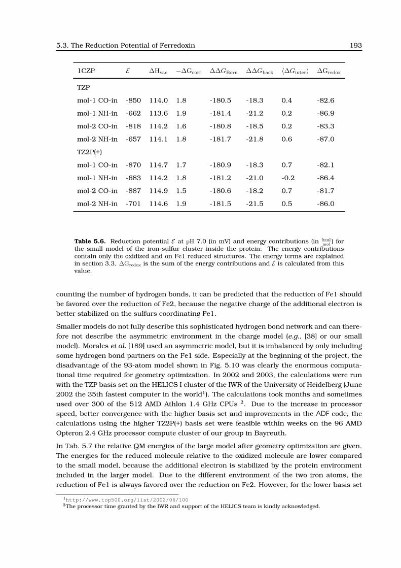
5.3. The Reduction Potential of Ferredoxin 193
1CZP E ∆Hvac −∆Gcorr ∆∆GBorn ∆∆Gback 〈∆Ginter〉 ∆Gredox
TZP
mol-1 CO-in -850 114.0 1.8 -180.5 -18.3 0.4 -82.6
mol-1 NH-in -662 113.6 1.9 -181.4 -21.2 0.2 -86.9
mol-2 CO-in -818 114.2 1.6 -180.8 -18.5 0.2 -83.3
mol-2 NH-in -657 114.1 1.8 -181.7 -21.8 0.6 -87.0
TZ2P(+)
mol-1 CO-in -870 114.7 1.7 -180.9 -18.3 0.7 -82.1
mol-1 NH-in -683 114.2 1.8 -181.2 -21.0 -0.2 -86.4
mol-2 CO-in -887 114.9 1.5 -180.6 -18.2 0.7 -81.7
mol-2 NH-in -701 114.6 1.9 -181.5 -21.5 0.5 -86.0
Table 5.6. Reduction potential E at pH 7.0 (in mV) and energy contributions (in kcalmol
) forthe small model of the iron-sulfur cluster inside the protein. The energy contributionscontain only the oxidized and on Fe1 reduced structures. The energy terms are explainedin section 3.3. ∆Gredox is the sum of the energy contributions and E is calculated from thisvalue.
counting the number of hydrogen bonds, it can be predicted that the reduction of Fe1 shouldbe favored over the reduction of Fe2, because the negative charge of the additional electron isbetter stabilized on the sulfurs coordinating Fe1.
Smaller models do not fully describe this sophisticated hydrogen bond network and can there-fore not describe the asymmetric environment in the charge model (e.g., [38] or our smallmodel). Morales et al. [189] used an asymmetric model, but it is imbalanced by only includingsome hydrogen bond partners on the Fe1 side. Especially at the beginning of the project, thedisadvantage of the 93-atom model shown in Fig. 5.10 was clearly the enormous computa-tional time required for geometry optimization. In 2002 and 2003, the calculations were runwith the TZP basis set on the HELICS I cluster of the IWR of the University of Heidelberg (June2002 the 35th fastest computer in the world1). The calculations took months and sometimesused over 300 of the 512 AMD Athlon 1.4 GHz CPUs 2. Due to the increase in processorspeed, better convergence with the higher basis set and improvements in the ADF code, thecalculations using the higher TZ2P(+) basis set were feasible within weeks on the 96 AMDOpteron 2.4 GHz processor compute cluster of our group in Bayreuth.
In Tab. 5.7 the relative QM energies of the large model after geometry optimization are given.The energies for the reduced molecule relative to the oxidized molecule are lower comparedto the small model, because the additional electron is stabilized by the protein environmentincluded in the larger model. Due to the different environment of the two iron atoms, thereduction of Fe1 is always favored over the reduction on Fe2. However, for the lower basis set
1http://www.top500.org/list/2002/06/1002The processor time granted by the IWR and support of the HELICS team is kindly acknowledged.

194 Examples for Ligand Binding Studies
S*1
F e 1F e 2
S*2*
S
O H
SN H
O
N H
O
N H
O
N H
O
N H
O
H N
N H
O
S
ON H
O
N H
N H
O
O H
S
O
H N
ON H
O
C 4 9
T 4 8S 4 7
C 4 6
A 4 5
G 4 4
A 4 3
R 4 2
C 4 1
S 4 0
C 7 9
T 7 8
Figure 5.10. Schematic representation of the large model containing the [2Fe-2S] center (inblue and yellow) and all backbone atoms of the two loops forming hydrogen bonds with theiron-sulfur cluster (black). Weak hydrogen bonds are dashed in black and strong hydrogenbonds are dashed in pink. The peptide bond between Cys46 and Ser47, which was observedin two conformations, is shown in red (including the additional hydrogen bond in the NH-in conformation). The sidechains of Thr48 and Thr78 (in green) can form hydrogen bondswith the iron-sulfur cluster, but they were omitted from the QM calculation to allow forrotameric freedom in the continuum electrostatic computations. Rotameric forms whichform hydrogen bonds with residues outside the large model are possible and maybe morelikely. The atoms marked by a circle were fixed in space during geometry optimization to beable to fit the optimized structure back into the protein.
TZP, the results fluctuate more than for the higher basis set TZ2P(+), so that the maximumdifference between equivalent forms in molecule mol-1 and mol-2 is 1.6 kcal
mol for TZP, but only0.5 kcal
mol for TZ2P(+). According to the QM energies, reduction of the NH-in conformer requiresabout 3 kcal
mol less energy than reducing the CO-in conformer.
The calculated reduction potentials based on the large model (Tab. 5.8) are much closer to theexperimental results than for the small model, however, the reduction potentials are slightlytoo high. Again, the results for the higher basis set TZ2P(+) are better than the results forTZP compared to experiment and also in terms of consistency between mol-1 and mol-2. Stillthe energy for the NH-in conformer is lower than the CO-in conformer, but the calculatedreduction potentials for CO-in are much closer to the experimentally determined reductionpotentials.

5.3. The Reduction Potential of Ferredoxin 195
1CZP mol-1 mol-2
ox red Fe1 red Fe2 ox red Fe1 red Fe2
CO-in TZP 0.0 32.6 35.1 0.0 32.3 34.1
NH-in TZP 0.0 30.2 31.1 0.0 30.2 32.7
CO-in TZ2P(+) 0.0 33.5 36.9 0.0 33.7 37.4
NH-in TZ2P(+) 0.0 30.4 33.3 0.0 30.6 33.5
Table 5.7. Quantum chemical energies (in kcalmol
) relative to the oxidized form of the largemodel of the iron-sulfur cluster relative to the oxidized form.
In my calculations I observed, that the reduction potential is strongly influenced by the pro-tonation probability of Glu94. This residue, shows an unusual protonation behavior and theprotonation probability curve is largely shifted compared to solution. At pH 7.0 Glu94 hasa significant probability of being protonated (pKapp of 7.4, 9.1, 6.3 and 6.9 in mol-1 CO-in,mol-1 NH-in, mol-2 CO-in and mol-2 NH-in respectively). Because the crystal structure 1CZP(as all Anabaena Fdx structures) was determined at a low pH of 5.5, where glutamates havea significant probability of being protonated, it was taken into consideration, that the proto-nation of Glu94 could be an artifact of the structure. In fact, several acidic residues showincreased calculated pKapp values.
The simplest approach was to fix Glu94 in the deprotonated form during the electrostatic cal-culations. The results in Tab. 5.8 show clearly lower reduction potentials in better agreementwith experimental results at pH 7.0. For the CO-in conformer, nearly perfect agreement withthe results of Hurley et al. [186] could be obtained. The small remaining differences could beattributed either to other acidic groups, which are unrealistically stabilized in the protonatedform by the protein structure, but interact less with the iron-sulfur center, or to other smallinaccuracies in the calculation and reduction potential measurement.
A significant effort has been made to find an alternative set of sidechain rotamers in Fdx,which stabilizes Glu94 in its deprotonated form. Therefore, the Dunbrack rotamer libraryas implemented in Perl Molecule was used. Rotating Glu94 by about -120◦ to increasethe distance between the negatively charges [2Fe-2S] cluster and the carboxy group did notchange the protonation probability sufficiently. Only extensive modeling rotating the nega-tively charged Glu95 out of the vicinity of the carboxy group of Glu94 and rotating His92 intohydrogen bond distance with Glu94 lead to a sufficient stabilization of the deprotonated formof Glu94. By that, some positive electron density in the geometric shape of a carboxyl groupcould be used, which was not fitted when determining the structure 1CZP. Even the electrondensity of the new rotamer is much less than for the rotamer modeled by the crystallogra-phers, it might be an indication for an additional rotamer, which is only little occupied underthe low-pH conditions for which the structure was determined. However, such a rotamermight be dominating at higher pH.

196 Examples for Ligand Binding Studies
1CZP E ∆Hvac −∆Gcorr ∆∆GBorn ∆∆Gback 〈∆Ginter〉 ∆Gredox
TZP
mol-1 CO-in -323 32.6 -2.0 -121.1 -5.2 1.0 -94.7
mol-1 NH-in -198 30.2 -3.4 -119.5 -5.2 0.3 -97.6
mol-2 CO-in -245 32.3 -2.0 -121.5 -6.2 0.9 -96.5
mol-2 NH-in -241 30.2 -2.3 -120.3 -5.3 1.1 -96.6
TZ2P(+)
mol-1 CO-in -354 33.5 -2.1 -121.1 -5.4 1.1 -94.0
mol-1 NH-in -241 30.4 -2.0 -120.5 -5.2 0.7 -96.6
mol-2 CO-in -362 33.7 -2.2 -120.8 -5.8 1.3 -93.8
mol-2 NH-in -284 30.6 -1.9 -120.2 -5.4 1.3 -95.6
Glu94 fixed to be deprotonated, TZ2P(+)
mol-1 CO-in -380 33.5 -2.1 -121.1 -5.4 1.7 -93.4
mol-1 NH-in -289 30.4 -2.0 -120.5 -5.2 1.8 -95.5
mol-2 CO-in -371 33.7 -2.2 -120.8 -5.8 1.5 -93.6
mol-2 NH-in -289 30.6 -1.9 -120.2 -5.4 1.4 -95.5
Table 5.8. Reduction potential E at pH 7.0 (in mV) and energy contributions (in kcalmol
) forthe large model of the iron-sulfur cluster inside the protein. The energy contributions con-tain only the oxidized and on Fe1 reduced structures. The energy terms are explained insection 3.3. ∆Gredox is the sum of the energy contributions and E is calculated from thisvalue.
It has to be noted, that the energy of the NH-in conformer is much lower than the energy ofthe CO-in conformer. Not only that the difference in QM energy of reduced and oxidized Fdxis about 3 kcal
mol lower for NH-in, but also the absolute QM energy of the oxidized state is 8.2 kcalmol
and 7.0 kcalmol lower for NH-in in molecule mol-1 and mol-2, respectively. The QM calculations
seem to greatly over-estimate the energy of this additional hydrogen bond by about 10 kcalmol .
Therefore, the qualitative conclusion can be drawn, that it is possible to construct a setof rotamers, which stabilize a deprotonated Glu94 at neutral pH and this structure agreeswell with experimentally measured reduction potentials. The calculated absolute reductionpotentials are in much better agreement with experimental results than any other previousabsolute or relative calculation attempts. The asymmetric reduction behavior of the two ironatoms was calculated in agreement with Mossbauer and NMR spectroscopic data.

5.3. The Reduction Potential of Ferredoxin 197
CO
-inA
-500
-450
-400
-350
-300
-250
-200
-150
-100
-50
0E
0 2 4 6 8 10 12 14
pH
B
-500
-450
-400
-350
-300
-250
-200
-150
-100
-50
0
E
0 2 4 6 8 10 12 14
pH
C
-500
-450
-400
-350
-300
-250
-200
-150
-100
-50
0
E
0 2 4 6 8 10 12 14
pH
D
-500
-450
-400
-350
-300
-250
-200
-150
-100
-50
0
E
0 2 4 6 8 10 12 14
pH
NH
-in
E
-500
-450
-400
-350
-300
-250
-200
-150
-100
-50
0
E
0 2 4 6 8 10 12 14
pH
F
-500
-450
-400
-350
-300
-250
-200
-150
-100
-50
0E
0 2 4 6 8 10 12 14
pH
G
-500
-450
-400
-350
-300
-250
-200
-150
-100
-50
0
E
0 2 4 6 8 10 12 14
pH
H
-500
-450
-400
-350
-300
-250
-200
-150
-100
-50
0
E
0 2 4 6 8 10 12 14
pH
[2Fe-2S] ox [2Fe-2S] red1 [2Fe-2S] red2 Glu94 prot.
Figure 5.11. Reduction and protonation probability plots of the iron-sulfur center (largemodel, TZ2P(+)) and Glu94 in conformer CO-in (A - D) and conformer NH-in (E - H) ofmolecule mol-1 of structure 1CZP. The probability of the iron-sulfur center being oxidized(A and E), being reduced on Fe1 (B and F) and being reduced on Fe2 (C and G) is shown.Plots D and H give the probability of Glu94 being protonated. The color coding of theprobability 〈x〉 is identical to Fig. 5.6.
5.3.3 Advantages of Using Perl Molecule and QMPB
The examples in the first two sections of this chapter could have been done with Multiflex aswell, but already in the application calculating the pKa value of His15 in HPr the capabilityof QMPB to deal with more than two instances was of advantage. The interpretation of theresults was much more straight forward, than the procedures required for Multiflex (describedin section 3.5.1). For Fdx absolute reduction potential calculations were required, for whichno single program existed before (section 3.5.2). Even Multiflex3D, which allows the three di-electric regions required for this model, could not cope with the three instances required todescribe the [2Fe-2S] center in one oxidized and two reduced forms. A consistent treatmentof reduction and protonation events would have only been possible with major manual inter-vention using Multiflex3D. For systems like Fdx, the study of the dependence of the reductionor protonation probability dependent on more than one chemical potential is important, as itcan be seen in Fig. 5.11. The reduction potential of the [2Fe-2S] center depends significantlyon the protonation probability of other residues like Glu94 and vice versa.
The structure preparation of 1CZP with Perl Molecule was discussed in detail in section 4.6.4.With any other method the complex modeling task splitting the structure in four conformersand generating all the rotamer forms and charge forms would have been much more compli-cated and error prone. As discussed before, the method add hydrogen adds several hydrogenrotamers for residues like serine or threonine, one for each possible hydrogen bonding part-ner. Rotamer energies were assigned by the method setup rotamer sites according to a filecharmm.potentials, which in turn contains torsion potential files for each relevant torsionangle (appendix A.4.3). The torsion potential files were generated by incrementally changingthe torsion potential and calculating the energy with CHARMM.

198 Examples for Ligand Binding StudiesC
O-in
A
-500
-450
-400
-350
-300
-250
-200
-150
-100
-50
0
E
0 2 4 6 8 10 12 14
pH
B
-500
-450
-400
-350
-300
-250
-200
-150
-100
-50
0
E0 2 4 6 8 10 12 14
pH
C
-500
-450
-400
-350
-300
-250
-200
-150
-100
-50
0
E
0 2 4 6 8 10 12 14
pH
D
-500
-450
-400
-350
-300
-250
-200
-150
-100
-50
0
E
0 2 4 6 8 10 12 14
pH
NH
-in
E
-500
-450
-400
-350
-300
-250
-200
-150
-100
-50
0
E
0 2 4 6 8 10 12 14
pH
F
-500
-450
-400
-350
-300
-250
-200
-150
-100
-50
0
E
0 2 4 6 8 10 12 14
pH
G
-500
-450
-400
-350
-300
-250
-200
-150
-100
-50
0
E0 2 4 6 8 10 12 14
pH
H
-500
-450
-400
-350
-300
-250
-200
-150
-100
-50
0
E
0 2 4 6 8 10 12 14
pH
rotamer 1 rotamer 2 rotamer 3 rotamer 4
Figure 5.12. Probability plots of the four hydrogen rotamers of Thr48 in the CO-in con-former (A-D) and NH-in conformer (E-H) of molecule mol-1 of structure 1CZP. The colorcoding of the probability 〈x〉 is identical to Fig. 5.6. A schematic drawing of the hydrogenbond formed by each rotamer is laid on top of the probability plot. The distance in Abetween Thr48 (Oγ) and the acceptor atom is given.
The importance of including several rotamers is shown by probability plots of instances ofThr48 in Fig. 5.12. The residue is described by four rotamer forms, but only three are pop-ulated. In the fourth rotamer, the Thr48 (Hγ1) would point in the direction of Glu94 (Oε1),which is significantly further away than the other potential (weak) hydrogen bond acceptors(Fig. 5.12 D and H). In the CO-in conformer, if the iron-sulfur center is reduced (Fig. 5.11 B)and Glu94 is protonated (Fig. 5.11 D), the rotamer of Thr48 forming a hydrogen bond withCys46 (Sγ) is most likely (cyan area in Fig. 5.12 A, about 75%). If the iron-sulfur center isoxidized and Glu94 is deprotonated, the probability of this instance is only 25-30 % (yellowarea). Instead the rotamer forming a (weak) hydrogen bond with Glu94 (Oε2) gets more likely(30-35 %, Fig. 5.12 C). Surprisingly, a rotamer between the two hydrogen bonds has overwide areas of the pH and reduction potential space a probability of 30 - 40 % (Fig. 5.12 B). Therotamer was included, because it describes the interaction with Cys46 (O) in the NH-in con-former, but in case of the CO-in conformer Thr48 (Hγ1) is pointing in the direction of Ser47(HN). The overall doubly negative charge of the quantum center seems to over-compensate therepulsion of the positive partial charges on the two hydrogen atoms.
In case of the NH-in conformer, the second rotamer, in which Thr48 (Hγ1) is interacting withCys46 (O), is overall the most populated instance (Fig. 5.12 F, ≥ 50%). If the iron-sulfur centeris reduced (Fig. 5.11 F) and Glu94 is protonated (Fig. 5.11 H), the rotamer forming a hydrogenbond with Cys46 (Sγ) is also significantly populated (green-yellow area in Fig. 5.12 E, about40%) and instead, if the iron-sulfur center is reduced and Glu94 is protonated, the rotamerforming the (weak) hydrogen bond with Glu94 (Oε2) gets more likely (about 50 %, Fig. 5.12 H ).Inclusion of only a single rotamer form would bias the iron-sulfur center and Glu94 towards aparticular instance and therefore shift the reduction and protonation probability, respectively.
5.3. The Reduction Potential of Ferredoxin 199
Rotamers of sidechains can be generated by Perl Molecule using a rotamer database (sec-tion 2.4.2). The file format of the Dunbrack backbone dependent and backbone independentrotamer database (appendix A.5.3) can be read by the class dunbrack (section 4.6.3) usingthe method molecule::read rotamers. The method molecule::generate rotamers gener-ates all rotamers in the database for a particular residue of a chain given as input parameter.The method molecule::remove clashing rotamers removes rotamers, which are too closeto atoms of the background set or non-rotamer sites. A parameter can be given to scale theradii, which was thought to be useful to reduce the number of rejected rotamers. Some ro-tamers might be valid, if e.g., smaller hydrogen radii as in force fields would be used or ifsome relaxation of the neighborhood of the new rotamer would be included in the protocol.Alternatively, only particular rotamers can be constructed by giving a hash of rotamer clas-sification strings as third parameter for molecule::generate rotamers. As energy for therotamers, the rotamer probability stored in the database can be converted by Perl Molecule,or all energies are calculated separately and assigned to the rotamers in the QMPB input file.The rotamer energies derived from probabilities turned out not to be useful. Currently, thesupport for rotamers in Perl Molecule is limited, because the CHARMM energy function is notimplemented to obtain the rotamer energies easily. Also a program calculating Lennard-Jonesterms, i.e., an interaction energy matrix of different rotamers is lacking. However, includingthis terms into the energy function would be very simple. For my more qualitative study onpossible alternative rotamers and their effect on the reduction potential this improved energyfunction was not required.
5.3.4 Conclusions
By treating a larger part of the protein by QM methods, a higher basis set and a crystal struc-ture of higher resolution, absolute reduction potentials for Anabaena Fdx could be calculated,which are in much better agreement with measured values than previous results. Also for thefirst time the asymmetric environment of the two iron atoms was included sufficiently intocalculations leading to two energetically well separated reduced forms. The results are inagreement with the Mossbauer data on a localized mixed valence Fe2+/Fe3+ state. Also thereduced iron Fe1 is in agreement with NMR data. However, obtaining accurate energies by QMcalculations still remains a challenge. It seems that todays DFT functionals are not accurateenough for the purpose of this work. An additional problem is to derive accurate point chargesform the electron density calculated by the QM method. This problem has no unique solu-tion and different approaches find considerably different results. Certainly, the electrostaticcalculations critically depend on the set of point charges used.
Another problem is that reduction potentials are usually measured at pH 7, but no crystalstructure exists at this pH. The used crystal structure was determined at a pH of 5.5, atwhich acidic groups are likely to be protonated (especially in such an acidic protein as Fdxand with a negatively charge iron-sulfur center). Under such conditions, groups of acidicresidues arrange into orientations stabilizing a bound proton and by that leading to an in-creased pKa value compared to the groups separated in solution. Similarly, Glu94 adopts anorientation close to the negatively charged iron-sulfur cluster stabilizing its protonated form.Probably the residue would adopt a different orientation at higher pH. It seems that such pHdependent conformational changes are important in Fdx since a structure could be modeled,
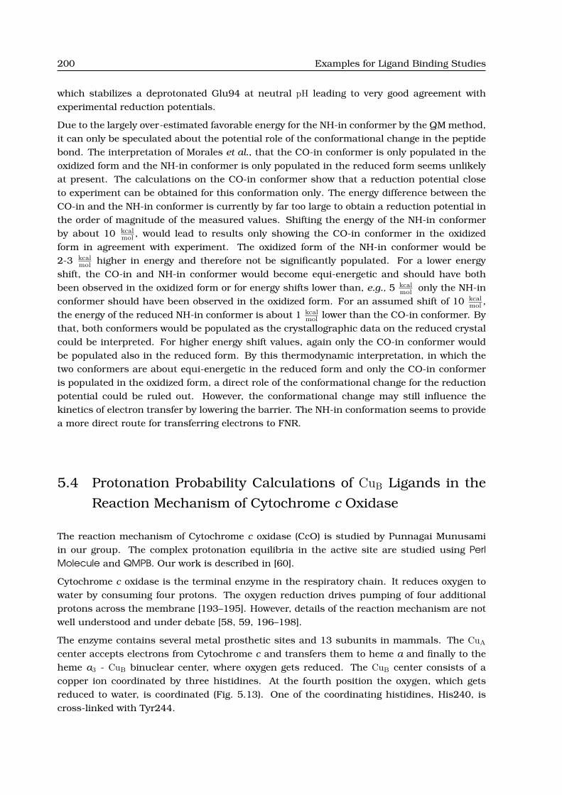
200 Examples for Ligand Binding Studies
which stabilizes a deprotonated Glu94 at neutral pH leading to very good agreement withexperimental reduction potentials.
Due to the largely over-estimated favorable energy for the NH-in conformer by the QM method,it can only be speculated about the potential role of the conformational change in the peptidebond. The interpretation of Morales et al., that the CO-in conformer is only populated in theoxidized form and the NH-in conformer is only populated in the reduced form seems unlikelyat present. The calculations on the CO-in conformer show that a reduction potential closeto experiment can be obtained for this conformation only. The energy difference between theCO-in and the NH-in conformer is currently by far too large to obtain a reduction potential inthe order of magnitude of the measured values. Shifting the energy of the NH-in conformerby about 10 kcal
mol , would lead to results only showing the CO-in conformer in the oxidizedform in agreement with experiment. The oxidized form of the NH-in conformer would be2-3 kcal
mol higher in energy and therefore not be significantly populated. For a lower energyshift, the CO-in and NH-in conformer would become equi-energetic and should have bothbeen observed in the oxidized form or for energy shifts lower than, e.g., 5 kcal
mol only the NH-inconformer should have been observed in the oxidized form. For an assumed shift of 10 kcal
mol ,the energy of the reduced NH-in conformer is about 1 kcal
mol lower than the CO-in conformer. Bythat, both conformers would be populated as the crystallographic data on the reduced crystalcould be interpreted. For higher energy shift values, again only the CO-in conformer wouldbe populated also in the reduced form. By this thermodynamic interpretation, in which thetwo conformers are about equi-energetic in the reduced form and only the CO-in conformeris populated in the oxidized form, a direct role of the conformational change for the reductionpotential could be ruled out. However, the conformational change may still influence thekinetics of electron transfer by lowering the barrier. The NH-in conformation seems to providea more direct route for transferring electrons to FNR.
5.4 Protonation Probability Calculations of CuB Ligands in the
Reaction Mechanism of Cytochrome c Oxidase
The reaction mechanism of Cytochrome c oxidase (CcO) is studied by Punnagai Munusamiin our group. The complex protonation equilibria in the active site are studied using PerlMolecule and QMPB. Our work is described in [60].
Cytochrome c oxidase is the terminal enzyme in the respiratory chain. It reduces oxygen towater by consuming four protons. The oxygen reduction drives pumping of four additionalprotons across the membrane [193–195]. However, details of the reaction mechanism are notwell understood and under debate [58, 59, 196–198].
The enzyme contains several metal prosthetic sites and 13 subunits in mammals. The CuA
center accepts electrons from Cytochrome c and transfers them to heme a and finally to theheme a3 - CuB binuclear center, where oxygen gets reduced. The CuB center consists of acopper ion coordinated by three histidines. At the fourth position the oxygen, which getsreduced to water, is coordinated (Fig. 5.13). One of the coordinating histidines, His240, iscross-linked with Tyr244.

5.4. Protonation Probability Calculations in Cytochrome c Oxidase 201
His291
His290His240
Tyr244
H O2
CuB
Figure 5.13. The model of the CuB center calculated by DFT. The Cβ atoms of the threehistidines were fixed in space at there crystallographic position (PDB code 2OCC [199]). Theatoms marked by white spheres were considered for deprotonation. Tyr244 is modeled as amethyl group.
Popovic et al. suggested that His291 deprotonates depending on the redox state of the CuB
center playing a central role in proton pumping [58, 59]. They found by DFT calculations thepKa value of His291 to be 8.6 and 13.2 in oxidized and reduced models of the CuB center inaqueous solution, respectively. Inside the protein pKa values of 4.0 and 19.7 were calculated.In contrast, Fadda et al. [196] obtained a pKa value of above 13.5 for His291 in the oxidizedstate, making a redox-coupled proton pumping involving this residue unlikely. The discrep-ancies led to some debate [197, 198] and weaknesses could be found in both studies: Thestructures were not fully relaxed in both studies leading to unrealistic bond lengths. Faddaet al. assumed standard protonation state for all amino acids in the protein. Both works alsostudied only the deprotonation of His291, but did not consider the other microstates of theCuB center to check for internal consistency.
We calculated all microscopic pKa values of the CuB center (Fig. 5.13) using DFT methods(Gaussian 03, B3LYP/6-31G*) and a conductor like polarizeable continuum model (C-PCM)[200–202] fixing only the Cβ carbons to their crystallographic positions. All titrateable aminoacids in the protein were allowed to adjust to the chemical potential and their environment.The eight microstates of the CuB center are shown together with the twelve microscopic pKa
values in Fig. 5.14. We obtained pKa values of 15.9 and 15.2 for the first deprotonation reac-tions of His290 and His291, respectively, in the oxidized state of the CuB center in aqueoussolution. Obviously, the pKa values are too high to allow deprotonation at physiological pHand the values are even higher in the reduced state. According to the QMPB calculations, alsoin the protein environment only the state is populated at pH 7, where His290, His291 andthe water molecule are protonated. Interestingly, however, the pKa value for deprotonating

202 Examples for Ligand Binding Studies
Cu+2.....H2OHis290.....HHis291.....H
His290.....HHis291.....H
Cu+2.....H2OHis290His291.....H
Cu+2.....H2OHis290.....HHis291
Cu+2.....H2OHis290His291
Cu+2......OHHis290His291.....H
Cu+2......OHHis290.....HHis291
Cu+2......OHHis290His291
Cu+2......OH
7.49.7
15.9
34.6
15.211.9
19.1
37.4
18.1
45.3
10.612.5
20.824.6
13.022.4
17.422.7
21.032.1
19.4
45.0
14.321.9
Figure 5.14. Microstates of the CuB center and microscopic pKa values in aqueous solution(blue) and in the protein with aquo-ferrous heme a3 (red).
His291 in the fully protonated state is the only pKa value, which drops by about 3 units, whileall other pKa values increase upon transfer from aqueous solution into the protein. Albeit thevalue is still too high to be deprotonated, it shows a tendency of the protein to lower the pKa
value specifically. A group with even higher pKa value could abstract the proton form His291.Tryptophane was suggested by us to fulfill this function, because it was recently discovered tobe involved in CcO reactions [203–206]. A possible mechanism could be, that a deprotonatedtryptophane radical is formed upon O-O bond cleavage. After rereduction, the tryptophanewith a solution pKa value of about 17 could protonate by abstracting a proton from His291.This model would allow a proton pumping mechanism as suggested by Popovic et al. [58], butonly in presence of a very strong base.
5.5 Reduction and Protonation Reactions of Quinones
Coenzyme Q plays a central role in a lot of biochemical processes, e.g., as electron and pro-ton carrier in photosynthesis, the mitochondrial respiratory chain, lysosomes, regulation ofphysicochemical membrane properties, as antioxidant and to regenerate other antioxidants,in aging to stimulate cell growth and inhibit cell death [207–209]. Due to the large number ofdifferent reduction and protonation states quinones are an ideal example of sites with manyinstances binding two different ligand types.
Ubiquinone is studied as a part of the bacterial reaction center by Eva-Maria Krammer inour group. However, ubiquinone has two flexible methoxy groups and a long (3-10 monomer)isoprenoid chain as substituents (Fig. 5.15 B). Therefore we chose the related organic moleculep-benzoquinone (Fig. 5.15 A) for quantum mechanical studies to determine an optimal methodto compute protonation and reduction equilibrium constants.
Due to the yellow color of p-benzoquinone and the colorless benzoquinol the reduction statecan be easily monitored by UV/VIS absorption spectroscopy. However, its poor solubility in
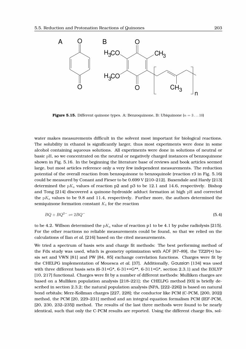
5.5. Reduction and Protonation Reactions of Quinones 203
O
O
n
O
O
O
O
CH
CH3
3
C
C
H3
H3
BA
Figure 5.15. Different quinone types. A: Benzoquinone, B: Ubiquinone (n = 3 . . . 10)
water makes measurements difficult in the solvent most important for biological reactions.The solubility in ethanol is significantly larger, thus most experiments were done in somealcohol containing aqueous solutions. All experiments were done in solutions of neutral orbasic pH, so we concentrated on the neutral or negatively charged instances of benzoquinoneshown in Fig. 5.16. In the beginning the literature base of reviews and book articles seemedlarge, but most articles reference only a very few independent measurements. The reductionpotential of the overall reaction from benzoquinone to benzoquinole (reaction r3 in Fig. 5.16)could be measured by Conant and Fieser to be 0.699 V [210–212]. Baxendale and Hardy [213]determined the pKa values of reaction p2 and p3 to be 12.1 and 14.6, respectively. Bishopand Tong [214] discovered a quinone-hydroxide adduct formation at high pH and correctedthe pKa values to be 9.8 and 11.4, respectively. Further more, the authors determined thesemiquinone formation constant K4 for the reaction
BQ+BQ2− 2BQ− (5.4)
to be 4.2. Willson determined the pKa value of reaction p1 to be 4.1 by pulse radiolysis [215].For the other reactions no reliable measurements could be found, so that we relied on thecalculations of Ilan et al. [216] based on the cited measurements.
We tried a spectrum of basis sets and charge fit methods: The best performing method ofthe Fdx study was used, which is geometry optimization with ADF [87–89], the TZ2P(+) ba-sis set and VWN [81] and PW [84, 85] exchange correlation functions. Charges were fit bythe CHELPG implementation of Mouesca et al. [37]. Additionally, Gaussian [134] was usedwith three different basis sets (6-31+G*, 6-31++G**, 6-311+G*, section 2.3.1) and the B3LYP[10, 217] functional. Charges were fit by a number of different methods: Mulliken charges arebased on a Mulliken population analysis [218–221]; the CHELPG method [93] is briefly de-scribed in section 2.3.2; the natural population analysis (NPA, [222–226]) is based on naturalbond orbitals; Merz-Kollman charges [227, 228]; the conductor like PCM (C-PCM, [200, 202])method, the PCM [20, 229–231] method and an integral equation formalism PCM (IEF-PCM,[20, 230, 232–235]) method. The results of the last three methods were found to be nearlyidentical, such that only the C-PCM results are reported. Using the different charge fits, sol-

204 Examples for Ligand Binding Studies
O−
O−
O−
−O
O
O
O
O
OH OH
OH
OH
BQ BQ
BQH −BQH
2−−BQ
2BQH
p1
e1 e2
p3
p2
e3
r1
r2
r3
Figure 5.16. Reduction (horizontal) and protonation (vertical) reactions of benzoquinone(BQ) to benzoquinole (BQH2). The intermediates are deprotonated benzosemiquinone(BQ−), protonated benzosemiquinone (BQH), singly deprotonated benzoquinole (BQH−)and doubly deprotonated benzoquinole (BQ2−). The reduction reactions are labeled e1 toe3 and the protonation reactions p1 to p3. Reactions r1 and r2 describe the uptake of ahydrogen radical, H ., and r3 the formal uptake of H2. The positively charged reaction inter-mediates were excluded from the study, because no experimental or theoretical data couldbe found for comparison.

5.5. Reduction and Protonation Reactions of Quinones 205
Figure 5.17. The energies (in kcalmol
) of the six microstates of BQ (shown in Fig. 5.16) areplotted for three basis sets and five charge fitting methods relative to the BQ microstate.The experimental data (or data calculated based on experimental data) is marked by redcrosses. The bars indicating the energy of the microstates are connected by lines, becausethe height of the bar would be hard to see otherwise, especially for the basis sets B3LYP/6-31+G* and B3LYP/6-311+G*.
vation energies were calculated using Solvate from the MEAD suite of programs, except for thePCM methods were solvation energies were taken directly form the Gaussian output.
The results for the microstate energies strongly depend on the charge fit method used. Theworst results were obtained with Mulliken and C-PCM charges, which lead to a difference inthe result of over 60 kcal
mol for BQ2− (Fig. 5.17). The difference due to different basis sets isnot that large, but discrepancies of over 5 kcal
mol are frequent. The triple split valence basis6-311+G* allows for more flexibility in the variation of PGTOs, than 6-31+G* and thereforeshould perform better. However, in all instances it performes equal or worse than the doublesplit valence basis set. A big improvement is gained from including polarization of the hydro-gen atoms and p-type diffusion functions. It seams reasonable, that for a molecule formed bys and sp2 orbitals, an accurate description of these orbitals by many functions is important.Clearly the charge fitting method with best agreement to experiment is NPA. For the unchargedforms BQH and BQH2 agreement within 1 kcal
mol with experiment could be obtained (-0.79 kcalmol
and 0.02 kcalmol , respectively; Fig. 5.18). For the charged instances BQH−, BQ− and BQ2− the
error is considerably larger (1.66 kcalmol , -8.18 kcal
mol and -6.63 kcalmol , respectively). As consequence,
the reaction free energies between the uncharged instances agree well (r1 -0.79 kcalmol , r2 0.81
kcalmol and r3 0.44 kcal
mol ). The calculation of r3 also compares favorably with the calculation ofWass et al. [14], who calculated the reaction energy by B3LYP/6-311+G** and IEF-PCM. Onlyafter correcting the gas phase reaction enthalpy by 8.3 kcal
mol according to experimental values,the error in the calculation reduced from -2.21 kcal
mol to -0.23 kcalmol .

206 Examples for Ligand Binding Studies
Figure 5.18. The microstate energies (in kcalmol
) are plotted as difference to the experimentalvalue and relative to the BQ microstate. The data is the same as in Fig. 5.17. The plot clearlyshows, that the NPA chargefit method together with B3LYP/6-31++G** is in particularlygood agreement with the experiment.
The first pKa value of BQH2 is reasonably predicted (error of 1.20 pKa units for p2, Fig. 5.19and Tab. 5.9), but the second pKa value and the pKa value of the semiquinone form have aconsiderable error (-6.05 pKa units for p3 and -5.39 pKa units for p1). An excellent agreementfor the p2 reaction was obtained by Liptak et al. [236] using a CBS-QB3 method with C-PCM.Our reduction potential calculations are considerably better for reducing the semiquinone(error of -67 meV for e2 and of -106 meV for e3) than for reducing BQ (error of 355 meV fore1).
It is remarkable, that the experimental values, which are probably the easiest to measure andtherefore the most accurate, i.e., r3 and p2 are among the best predicted reaction free energiesby Gaussian NPA. The pKa value of p3 is hard to measure in aqueous solution due to its highvalue and p1 due to the complex radical chemistry involved to generate the semiquinoneform. However, the calculated pKa value for p3 is unrealistic, because by chemical intuitionone would assume that the value should be higher than the value of p2, which only couldbe found using the PCM methods or ADF. Also a negative pKa value for p1 seems not tobe realistic, but clearly positive values could only be obtained using the PCM methods orADF as well. Therefore, the problem seems rather to be a systematic error in the calculationof charged instances by the QM method, than experimental inaccuracies. It can be hoped,that adding two or three diffusion functions to better describe the loosely bound electronsof charged species will resolve the remaining problems. Another option would be to choosea different experimental value from literature [237, 238] for the potential of the standardhydrogen electrode and the solvation energy of a proton, which are closely related quantities.We use the value of -260.5 kcal
mol [120] for the solvation energy of the proton in consistency with

5.5. Reduction and Protonation Reactions of Quinones 207
Figure 5.19. The reaction free energy difference (in kcalmol
) of the nine microscopic reactions(shown in Fig. 5.16) are plotted. Particularly good agreement is also here obtained by the6-31++g** basis set and the NPA chargefit method.
reaction Gaussian NPA ADF CHELPG experiment Reference
in units of kcalmol pKa eV kcal
mol pKa eV kcalmol pKa eV
e1 -10.39 7.6 0.451 12.20 -8.9 -0.529 -2.21 1.6 0.096
e2 1.02 -0.7 -0.044 0.78 -0.6 -0.034 -0.53 0.4 0.023
e3 -8.09 5.9 0.351 -11.61 8.5 0.503 -10.53 7.7 0.457
p1 1.78 -1.3 -0.077 -15.41 11.2 0.668 -5.62 4.1 0.244 [215]
p2 -15.14 11.0 0.656 -24.97 18.2 1.083 -13.49 9.8 0.585 [213, 214]
p3 -7.33 5.3 0.318 -27.80 20.2 1.205 -15.62 11.4 0.677 [213, 214]
r1 -8.61 6.3 0.373 -3.21 2.3 0.139 -7.82 5.7 0.339 [216]
r2 -23.22 16.9 1.007 -36.58 26.6 1.586 -24.03 17.5 1.042 [216]
r3 -31.83 23.2 1.380 -39.80 29.0 1.726 -32.26 23.4 1.398 [210–212]
Table 5.9. Calculated and experimental reaction energies in different energy units. Theexperimental value of 0.699 V per electron is doubled for the two electron, two proton reac-tion r3. The RMSD for the Gaussian B3LYP/6-31++G** calculations is 1.58 kcal
mol, for the ADF
TZ2P(+) calculations 3.19 kcalmol
relative to the experimental values. Experimental values weremeasured for p1, p2, p3 and r3. Ilan [216] calculated r1 and r2 based on these experimentalvalues and we added e1, e2 and e3 following the thermodynamic cycle in Fig. 5.16.
208 Examples for Ligand Binding Studies
older works [13, 38, 126] using ADF. Instead, in the work on CcO, Punnagai Munusami useda value of -264.61 kcal
mol [236, 239], which seems to work better with Gaussian C-PCM.
The problems arising for the rather simple organic molecule p-benzoquinone highlight thechallenge to compute reaction free energies in complex metall clusters, like the [2Fe-2S] clus-ter of Fdx and the CuB center of CcO. In both projects QM methods were used, which performsignificantly worse for p-benzoquinone. However, at the moment it seems, that different meth-ods are good for different molecules, i.e., higher basis sets and using NPA gave worse resultsfor the CuB center. It is questionable, if the currently used GTO basis sets, polarization anddiffusion functions are high enough to describe metal centers as in Fdx as accurate as theTZ2P(+) STO basis set of ADF. Therefore, future work has to investigate further, which methodis suitable for a broad spectrum of molecules to obtain accurate reaction free energies.
5.6 Proton Transfer Through the Gramicidin A Channel
A Dynamical Monte Carlo algorithm (DMC) was developed in the group by Mirco Till, TorstenBecker and Matthias Ullmann. This algorithm allows to study transfer processes inside pro-teins, i.e., long range proton transfer reactions. On the basis of electrostatic energies cal-culated by QMPB, probabilities of transitions between microstates within a time interval arecalculated. My contribution to the work was on one hand assistance in setting up the systemfor QMPB calculations. since the results of the QMPB calculation were a necessary input forthe DMC calculations. On the other hand I contributed some ideas on an efficient cachingalgorithm (section 4.2.2) speeding up the simulation time by a factor of 13 and thus makingsimulations on the model system gramicidin A (gA) possible with acceptable computational ef-fort. A manuscript describing the DMC algorithm and the application on gA is in preparation[240].
The study of long range proton transfer processes is important in many biological processes,e.g., the generation of a proton gradient across a membrane in photosynthesis and respiration.The theoretical study of such processes was hindered on one hand by the inability of standardMD simulations to incorporate proton binding and release reactions, on the other hand by thetime scale of microseconds to milliseconds required for such proton transfer processes. Whilethe time scale imposes a challenge to MD simulations, it is not feasible with QM/MM methodsallowing for bond-breaking and -forming. The DMC approach combines electrostatic calcula-tions in the grand canonical ensemble, which seamlessly allows ligand binding reactions (e.g.,protonation probability calculations), with a master equation to describe the time evolutionof the system. A Monte Carlo approach is applied to approximate the solution of the masterequation.
The microstate energy is described in section 3.1.2 extended by an additional term to theintrinsic energy describing the contribution due to a membrane potential [39]. The equilibriumprobability of a particular state is given by eq. 3.9, including the membrane potential into the
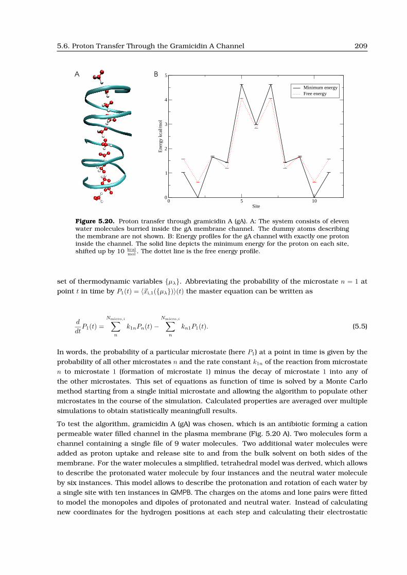
5.6. Proton Transfer Through the Gramicidin A Channel 209
A
0 5 10Site
0
1
2
3
4
5
Ene
rgy
kcal
/mol
Minimum energyFree energy
B
Figure 5.20. Proton transfer through gramicidin A (gA). A: The system consists of elevenwater molecules burried inside the gA membrane channel. The dummy atoms describingthe membrane are not shown. B: Energy profiles for the gA channel with exactly one protoninside the channel. The solid line depicts the minimum energy for the proton on each site,shifted up by 10 kcal
mol. The dottet line is the free energy profile.
set of thermodynamic variables {µλ}. Abbreviating the probability of the microstate n = 1 atpoint t in time by P1(t) = 〈~xi,1({µλ})〉(t) the master equation can be written as
d
dtP1(t) =
Nmicro,i∑n
k1nPn(t)−Nmicro,i∑
n
kn1P1(t). (5.5)
In words, the probability of a particular microstate (here P1) at a point in time is given by theprobability of all other microstates n and the rate constant k1n of the reaction from microstaten to microstate 1 (formation of microstate 1) minus the decay of microstate 1 into any ofthe other microstates. This set of equations as function of time is solved by a Monte Carlomethod starting from a single initial microstate and allowing the algorithm to populate othermicrostates in the course of the simulation. Calculated properties are averaged over multiplesimulations to obtain statistically meaningfull results.
To test the algorithm, gramicidin A (gA) was chosen, which is an antibiotic forming a cationpermeable water filled channel in the plasma membrane (Fig. 5.20 A). Two molecules form achannel containing a single file of 9 water molecules. Two additional water molecules wereadded as proton uptake and release site to and from the bulk solvent on both sides of themembrane. For the water molecules a simplified, tetrahedral model was derived, which allowsto describe the protonated water molecule by four instances and the neutral water moleculeby six instances. This model allows to describe the protonation and rotation of each water bya single site with ten instances in QMPB. The charges on the atoms and lone pairs were fittedto model the monopoles and dipoles of protonated and neutral water. Instead of calculatingnew coordinates for the hydrogen positions at each step and calculating their electrostatic

210 Examples for Ligand Binding Studies
interaction with the environment, this discrete model allows to pre-compute all energies forall permutations of protons and lone pairs in the tetrahedral coordinate system of each watermolecule. This approximation leads to a dramatic time saving making the simulations possibleat all.
Nevertheless, 1011 microstates (11 water molecules with 10 instances each) remain, for whichsets of reaction rates and probabilities need to be calculated. Here the caching algorithm dis-cussed in section 4.2.2 together with several other optimizations turned out to be valueable.
An energy profile for the transfer process can be obtained (Fig. 5.20 B), showing that theenergy barrier for the long range proton transfer through the gA channel is about 3.4 kcal
mol
for the free energy profile and 4.6 kcalmol for the minimum energy profile. The DMC approach
allows to simulate the proton transfer through gA on a microsecond to millisecond timescale.The calculated proton flux reproduces experimentally derived values over a wide range ofpH values and membrane potentials (see [240]). The calculations indicate, that the rate of theproton transfer is limited by the gaps between the proton transfer events, not by transfer timesof single protons. For physiological membrane potentials, the electrostatic energy barrier isprobably the rate limiting factor for a single proton transfer and not the orientation of thehydrogen bonded network. However, both factors influence the rate constants at the sameorder of magnitude and are therefore important for the long range proton transfer process.

CHAPTER 6
CONCLUSIONS AND OUTLOOK
In my thesis the commonly used theory of ligand binding energetics was generalized to allowfor any number of ligand types, which can bind to any number of sites having any numberof instances. A consistent microstate description is given in the grand canonical ensemble toallow treatment of sites parameterized based on experimental data or on quantum mechanicalcomputations. The choice of a different reference state led to a significant simplification of theequations compared to previous formulations of the less general energy function. Focussingon ligand binding reactions as function of the chemical potential of the ligand type in the bulksolvent renders the equations more concise, while making them more general at the sametime. Previous formulations were increasing in complexity with the number of ligand types,e.g., adding terms for the pKa value and the reduction potential calculation. They led to someconfusion of the sign of values due to the definition of the pKa value based on a deprotonation(unbinding) reaction, while the standard reduction potential refers to the binding reaction ofelectrons. The discussion based on energies in common units (e.g., kcal
mol ) makes it easier tocompare contributions and avoids odd results, e.g., reduction potentials in pKa units.
An important contribution to the energy function are electrostatic terms calculated by solvingthe Linearized Poisson-Boltzmann (LPBE) equation. Classifying the electrostatic energies ashomogeneous and heterogeneous transfer energies dependent on the origin of the transfermade the equations more compact. Sites can be parameterized by calculating the energy offormation and vibration quantum mechanically (QM). The electrostatic contributions are ahomogeneous transfer energy (from vacuum into the protein) and a correction energy to ex-clude electrostatic interactions, which are also usually excluded in force-field calculations.For each ligand an energy of the free ligand in bulk solution is included. This term includessome experimental value (e.g., the solvation energy of a proton or the potential of the standardhydrogen electrode) and potentially the energy of formation of the ligand as well as entropyestimates of the binding reaction or energy terms related to volume work. So called relative lig-and binding energy calculations rely on the experimentally determined ligand binding energyof model compounds in solution for parameterizing sites. The LPBE calculation determinesthe shift of the binding energy upon transferring the site from the model compound into theprotein environment. Since the rotamers are usually not determined together with the ligandbinding energy, energy contributions for changing the rotamer form must be estimated e.g.,by a molecular mechanics (MM) force field. Details of the calculation vary if the instance is areference rotamer or not, or if no rotamers are included for this site at all.
211

212 Conclusions and Outlook
Ligand binding calculations are usually done in three steps: First, the three dimensionalstructural information of the molecule of interest, known by x-ray crystallography or NMRspectroscopy, is processed to prepare a format suitable for further computations. This stepcan be rather simple for simple molecules, e.g., transferring the cartesian coordinates for eachatom into a file and adding charges from a force field, but it can also be the most complicatedstep of the calculation, if substantial modeling is necessary. Previously, this step was mainlyleft to the user to do manually or to write own scripts. This approach led to a substantialamount of repetitive work and was a major source of errors.
For the purpose of structure preparation and input generation an object library, Perl Mole-cule, was written, which allows to write short Perl programs doing all necessary steps. Sincepowerful object library methods are used, mistakes by the user are less likely. The structurepreparation is easier to control and the protocol is transferable to similar proteins. However,the design as a library or tool box allows to implement variations on the protocol easily and isopen for future extensions.
The second step is the calculation of electrostatic energies. For this purpose QMPB waswritten, which is an interface to programs solving the LPBE. By separating the interfacefrom the Poisson-Boltzmann solver, the PB solver library can be exchanged with little effort.QMPB is minimalistic by design, relying on one side on proper input preparation by a pre-processor program and on the other side on an external PB solver. By this design it shouldbe easy to adopt QMPB to changing energy functions, e.g., additional energy terms foundto be necessary to include. At the same time it should be as flexible as the equations forligand binding. All complexity, which may arise from complicated sites, is left to the pre-processor. QMPB concentrates on implementing the energy functions as general as they werederived. All calculation steps should be transparent to the user to follow each step and detectpossible mistakes. Each calculation step can be reproduced by the user for education anderror checking. However, for non-trivial systems the number of analogous steps is too largeto be done manually requiring a program like QMPB.
QMPB scales linear with the total number of instances of the system. Since the LPBE cal-culations of instances are independent of each other, parallel execution on any number ofprocessors is possible without any inter-processor communication. Therefore, linear scal-ing with the number of processors up to the total number of instances, which ranges fromsome hundred to several thousand for biological systems, is expected. The parallelization oradoption to particular computing environments does not require any changes in the QMPBprogram, but can be done by external scripts or programs dependent on the local require-ments. This separation of the parallelization from the main program is another advantage ofthe design decision to perform the LPBE calculations by external programs.
The third step in the calculation is to calculate ligand binding probabilities dependent on ther-modynamic variables, i.e., sets of chemical potentials of ligands in the bulk solvent. For verysmall systems an analytical evaluation of the partition function is possible and can be per-formed, e.g., by SMT1. For larger systems ligand binding probabilities have to be approximated,which can be done by a Monte Carlo procedure as implemented in GMCT1. The programs relyon the intrinsic energies and interaction energies calculated and tabulated by QMPB. Forlarger systems, especially with more than one or two ligand types, the Monte Carlo procedure
1SMT and GMCT were written by Matthias Ullmann.

213
is the time limiting step of the whole calculation. Parallelization can help to reduce the wall-clock time a user needs to wait, but the computational effort increases exponentially with thenumber of ligand types. With the Adaptive Mesh Refinement (AMR) algorithm suggested inthis work a substantial saving of computational time on the calculation of probabilities can beexpected. The probability of most instances is constant over wide areas in chemical potentialspace, e.g., only the fraction of the chemical potential range, where the instance titrates, isof interest to be sampled by a fine grid. Also the correlation with other sites binding otherligands is usually not strong, so that instances tend to be rather constant in dimensions ofchemical potential space representing ligands not binding to this site. Therefore, an algorithmexploiting these properties can reduce the computational cost substantially.
Currently, the savings by AMR are still modest, which is in part due to the test system cho-sen, which represents a kind of worst case scenario, and in part due to limitations in theimplementation, not fully exploiting the power of the algorithm. At present, titration calcula-tions are only done up to two dimensions, but many current and future projects of the groupwill demand studies of more ligand types. The generalized theory and QMPB permit usingany number of ligand types, but the exponential scaling behavior of the Monte Carlo proce-dure will become a hindrance. Therefore, future work on AMR and similar approaches will bevalueable and strongly required.
My implementation of the ligand binding theory does not include membrane potentials, be-cause my primary focus was on soluble proteins. The theory of including membrane potentialsin electrostatic potentials was worked out by Elisa Bombarda. Thomas Ullmann extendendthe LPBE solver libraries of MEAD by a sophisticated membrane model and functions to in-clude membrane potentials. Since the membrane potential can be described by an additiveterm to the intrinsic energy in my equations, it was easy to replace the external LPBE solverprograms by those being able to perform membrane potential calculations. Here the modulardesign already proved to be usefull. Future versions of Perl Molecule and QMPB should beable to prepare also the input for membrane proteins, which is currently done by externalhelper programs. In the probability calculation of instances, the internal and external chemi-cal potential of protons will be treated as different ligand types and therefore contribute to thescaleability problem of the Monte Carlo calculation step.
The current implementation of rotamers in Perl Molecule is probably good for hydrogen atoms.However, the group of Marylin Gunner and others have shown, that including sidechain ro-tamers can help to improve on the agreement between calculated and experimentally mea-sured pKa values. Probably sidechain flexibility can also help in binding studies of otherligands. Currently, the support for sidechain rotamers by Perl Molecule is quite limited, be-cause no force field energy function is implemented. The energies derived from probabilities ofrotamers in databases was not found to be meaningfull and tabulating pre-computed rotamerenergies by an external program is not feasible for longer sidechains. Also the interaction withthe protein environment as well as with other rotateable sidechains needs to be included. Theformalism of QMPB splitting the energy function in an intrinsic energy independent of allother sites and an interaction term accounting for the pairwise interactions of two instancesof two sites can remain. Just an additional program is required calculating these energy con-tributions. This program could also solve the problem of the omitted Lennard-Jones termsin the current implementation, which is probably negligible for hydrogen rotamers, but getsimportant for sidechain rotamers. Also in this direction work is done by Thomas Ullmann.

214 Conclusions and Outlook
Perl Molecule and QMPB have proven to be usefull in a number of projects outlined in theapplication section. In fact, most members of the group are currently using QMPB for theirresearch and it has already become a part of the research practical for students to learn usingit. The programs should be made available for any interested user via the internet under theGPL, free of charge allowing to modify and extend the programs for future applications.
However, the applications of QMPB to sites parameterized by quantum chemical calculationshas not yet provided fully reliable results. In fact, it was expected to be one of the mainadvantages of QMPB to be able to treat sites, which can not sufficiently be characterized byexperiment. In this field it is to my knowledge also the only program so far, which can satis-fyingly solve the multiple site titration problem. Actually, the problems which arose, are notdirectly related to Perl Molecule or QMPB, but are rooted in the limitations of current chargefitting methods and inaccuracies of currently available basis sets and exchange correlationfunctionals. Since QMPB takes only the charges and energies no matter which way they weredetermined, it is open to any new development in the field of quantum chemistry.
By no means, the formalism and implementation of my programs is limited to thermody-namics of ligand binding only. As the application on gramicidin A shows, QMPB suites wellto provide the thermodynamic basis for further kinetic studies on ligand transfer reactions.Currently work is done by Eva-Maria Krammer and Mirco Till applying DMC to proton trans-fer reactions in the bacterial reaction center and future projects may include electron transferreactions as well. Other applications of QMPB have been stability predictions of proteins aftersite directed mutagenesis. Different amino acids at a position can be treated as different in-stances. Also for such projects, inclusion of better energy terms for sidechain rotamers is ofinterest.
Since already in such a short time Perl Molecule and QMPB have proven to be usefull fordifferent projects in the domain of applications, for which they were written, and outsideof this domain, it can be expected that the programs will be of great use in the theoreticalbiophysics community as soon as they will be made available to a larger group of users.

NOMENCLATURE
Here the meaning of certain terms is explained as they are used in this thesis and in thePerl Molecule ontology. However, no general definitions are attempted.
atomAtom in a particular residue of a chain and conformer of the biomolecule. An atom isdescribed by a radius (r in A), a set of coordinates and a set of charges.
background (charge) setSet of atoms of a conformer, which does not belong to any site.
background energyEnergy of a charge due to interaction with fixed charges in the system (backgroundcharges).
binding free energyFor a molecule the binding energy is the difference in microstate energy of the boundand unbound microstate. For a site the binding energy is the difference in energy of thebound and unbound instance of the site.
Born energyEnergy of a (solvated) charge due to a set of dielectric boundaries.
chainUsually identical with a polymer chain of the biomolecule in a particular conformer. Achain is a set of residues.
charge formSet of atoms with their respective partial charges keeping an integer total charge. Definedby a column in a charge set file (appendix A.2).
charge group memberAdditional information associated with an atom defined in a topology file (appendixA.5.1). Most important is the partial charge.
charge groupSet of charge group members with their respective partial charges keeping an integertotal charge. Charge groups are usually defined by topology files (appendix A.5.1).
215

216 Nomenclature
chargePartial charge q of an atom in units of a fraction of an elementary charge.
charge setSet of charge forms. Defined by a charge set file, see appendix A.2.
conformationSynonymous with conformer, i.e., globally different structure.
conformational energyThe conformational energy is the energy of a particular conformation relative to a refer-ence conformation.
conformerDiscrete conformation, i.e., globally different structure. Independent sets of electrostaticcalculations (with different sets of dielectric boundaries) need to be performed for eachconformer. A conformer is a set of chains.
coordinateCartesian coordinate of an atom (x, y, z in A).
coordinate setSet of rotamer forms.
instance memberParticular, single atom with coordinates and charges taken from a particular combina-tion of rotamer form and charge form.
instanceSet of atoms with coordinates and charges taken from a particular combination of ro-tamer form and charge form.
interaction energyThe interaction energy is due to the interaction of the potential of an instance of a sitewith the charges of an instance of another site.
intrinsic energyThe intrinsic energy is the energy of an instance of a site in the dielectric boundaries ofthe molecule and interacting with the background (charge) set. The charges of all atomsbelonging to another site are set to zero.
microstate energyEnergy of a molecule in a particular microscopic state at a given set of thermodynamicvariables.
moleculeBiomolecular system, e.g., a ribosome. A molecule is described as set of conformers.Because all studies concentrated on proteins, “protein” is often used synonymouslywith biomolecule, not excluding that the described methods can be applied to otherbiomolecules as well..

Nomenclature 217
reaction fieldEffective electrostatic field acting back on the charge, which created the field.
reaction free energyThe reaction free energy is the energy difference of the system before and after a reaction.
residueUsually identical with a residue of the biopolymer in a particular chain and conformer.A residue is a set of atoms.
rotamer formSet of atoms with their respective coordinates.
siteSet of atoms associated with a coordinate set and/or charge set. A site is a set of in-stances.
solvation energyHomogeneous transfer energy from vacuum into a given solvent.
state vectorVector characterizing a microstate. The length of the state vector equals the number ofsites and the value at each position refers to a particular instance of the site.
Stern layerIon exclusion layer around the protein to preserve a solvation layer around the ions.

218

ABBREVIATIONS AND ACRONYMS
cre Carbon catabolite response element.
ADF Amsterdam density functional.
AMBER Assisted model building and energy refinement.
AMD Advanced Microdevices.
AMR Adaptive mesh refinement.
APBS Adaptive Possion-Boltzmann solver.
API Application programming interface.
ASCII American standard code for information interchange.
ATP Adenosine triphosphate.
AWK Interpreter language named by the authors Alfred Aho, PeterWeinberger and Brian Kernighan.
B. subtilis Bacillus subtilis.
C-PCM Conductor like PCM.
cAMP Cyclic adenosine monophosphate.
CcO Cytochrome c oxidase.
CcpA Carbon catabolite control protein A.
CCR Carbon catabolite repression.
CHARMM Chemistry at Harvard macromolecular mechanics.
CHELP Charges from electrostatic potentials.
219

220 Abbreviations
CHELPG Charges from electrostatic potentials using a grid based method.
CMCT Conformational Monte Carlo titration.
COSMO Conductor like screening model.
CPAN Comprehensive Perl archive nework.
CPU Central processing unit.
DelPhi Finite difference Poisson-Boltzmann solver by the Honig labora-tory.
DFT Density functional theory.
DHC2 Diheme cytochrome c2.
DMC Dynamical Monte Carlo.
DMF Dimethylformamide.
DNA Deoxyribonucleic acid.
E. coli Escherichia coli.
e.s.u.-c.g.s Electrostatic units based on centimeter, gram, second and otherbase units.
EI Enzyme I.
EII Enzyme II.
EIII Enzyme III.
EVB Empirical valence bond method.
Fdx Ferredoxin.
FIFO First in first out buffer.
FNR Ferredoxin-NADP-oxidoreductase.
FORTRAN Formula translation.
gA Gramicidin A.
GAMESS General atomic and molecular electronic structure system.

Abbreviations 221
GMCT Generalized Monte Carlo titration.
GNU GNU is not Unix.
GPL GNU public license, http://www.gnu.org/copyleft/gpl.html.
GREP Global regular expression print.
GROMACS Groningen machine for chemical simulations.
GTO Gaussian type orbital.
HELICS Heidelberg Linux cluster system.
HEWL Hen egg white lysozyme.
HF Hartree-Fock.
HPr Histidine-containing phosphocarrier protein.
HPrK/P HPr Kinase/Phosphatase.
IEF-PCM Integral equation formalism PCM.
IO Input/output.
IPC Interprocess communication.
IR Infrared spectroscopy.
IWR German: Institut fur wissenschaftliches Rechnen, English: Insti-tute for scientific computing.
KS Kohn-Sham.
LCAO Linear combination of atomic orbitals.
LPBE Linearized Poisson-Boltzmann equation.
LSDA Local spin density approximation.
MC Monte Carlo.
MCCE Multiconformational continuum electrostatics.
MCTI Monte Carlo titration.

222 Abbreviations
MD Molecular dynamics.
MD-PDLD Molecular dynamics averaging of PDLD calculations.
MDC Multipole derived charges.
MEAD Molecular electrostatics at atomic detail.
MEP Molecular electrostatic potential.
MM Molecular mechanics.
MMC Metropolis Monte Carlo.
MPI Message passing interface.
NADP Nicotinamide adenine dinucleotide.
NMR Nuclear magnetic resonance spectroscopy.
NOE Nuclear Overhauser effect.
NPA Natural population analysis.
NUMA Non-uniform memory access or architecture.
OMG Object Management Group.
OOP Object-oriented programming.
PARSE Parameters for solvation energies.
PB Poisson-Boltzmann.
PBE Poisson-Boltzmann equation.
PCM Polarizable continuum model.
PDB Protein data bank.
PDLD Protein dipoles Langevin dipoles.
PEP Phosphoenolpyruvat.
Perl Practical extraction and report language.
PGTO Primitive Gaussian type orbital.
PTS Phosphoenolpyruvat:sugar phosphotransferase system.

Abbreviations 223
PVM Parallel virtual machine.
PW Gradient-corrected XC energy functional of Perdew and Wang.
QM Quantum mechanics (here synonymously used with quantumchemistry).
QMPB Quantum mechanics based Poisson-Boltzmann.
RAID Redundant array of inexpensive disks.
RAM Random access memory.
RMSD Root mean square deviation. The RMSD is used as a measure forsimilarity. It is calculated by
RMSD =
√∑ni=1(~rai − ~rbi)2
n, (6.1)
where ~rai and ~rbi are the positions of atom i of structure a andb, respectively. The number of atoms if given by n. In this work,RMSD is also used for scalars synonymously with a standard de-viation.
RNA Ribonucleic acid.
SCF Self-consistent field.
SCSI Small computer systems interface.
SED Stream editor.
SHE Standard hydrogen electrode.
SI International system of units based on kilogram, meter, second,ampere, kelvin, mole, candela.
SMP Symmetric multiprocessor architecture.
SMT Statistical mechanics treatment.
SOR Successive over-relaxation.
SPE Synergistic processing elements.
STO Slater type orbital.
SVD Singular value decomposition.

224 Abbreviations
SWIG Simplified wrapper and interface generator.
TZ2P Core double-ζ, valence triple-ζ, doubly (2) polarized basis set ofADF.
TZ2P(+) TZ2P+ for transition metals Sc-Zn and TZ2P otherwise.
TZ2P+ As TZ2P, but with 4 d-functions instead of 3 (only for transitionmetals Sc-Zn).
TZP Core double-ζ, valence triple-ζ, polarized basis set of ADF.
UHBD University of Houston Brownian Dynamics.
UML Unified modeling language.
UV Ultra violet light absorbtion spectroscopy.
VIS Visual light absorbtion spectroscopy.
VMD Visual molecular dynamics.
VWN LSDA parameterization of Vosko, Wilk and Nusair.
XC Exchange and correlation.
XML Extensible markup language.

EQUATION SYMBOLS
E[ρ(~r)] Energy functional.
EXC [ρ(~r)] Exchange and Correlation Energy.
E Total energy.
GBorn,homo,i(jk) Born energy of instance jk in the homogeneous environment.
GBorn,model,i(jk) Born energy of instance jk in the model compound.
GBorn,protein,i(jk) Born energy of instance jk in the protein.
GBorn Born energy.
Gback,homotrans,i(jk) Background energy of instance jk in the protein.
Gback,model,i(jk) Background energy of instance jk in the model compound.
Gback,protein,i(jk) Background energy of instance jk in the protein.
Gback Background energy.
Gtrans(H+) Translational energy of the proton.
Gconf,i Conformational energy of conformer i.
Gcorr,i(jk) Correction of the background energy of instance k of site i in con-former i.
Gfree,i(jk) Energy of the unbound ligand molecules for instance k of site i inconformer i.
Ginter,i(jk, lm) Interaction energy of instance k of site i with instance m of site lin conformer i.
Gintr,i(jk) Intrinsic energy of instance k of site i in conformer i.
Gmicro Energy of a particular microstate.
Gvib,i(jk) Vibrational energy obtained from QM calculations on instance k
of site i in conformer i.
225

226 Equation Symbols
Hvac,i(jk) Total bonding energy (or energy of formation) obtained from QMcalculations on instance k of site i in conformer i.
H Hamiltonian.
I Ionic strength.
NA Avogadro constant.
Nϑ Number of electrons with spin ϑ = α, β.
Ne Number of electrons.
Nλ Number of ligands λ bound to conformer i of the molecule.
Natom Number of atoms in the molecule.
Nback,i Number of atoms in the background set of conformer i.
Nback,model,i,j Number of atoms in the background set of the model compoundfor site j of conformer i.
Nconf Number of conformers.
Niontype Number of ion types.
Ninstance,i,j Number of instances in site j in conformer i.
Ninstance,i,l Number of instances in site l in conformer i.
Nligand Total number of reactive ligand types λ.
Nmicro,i Number of microstates in conformer i.
Nmoves Total number of MC moves.
Nscans Total number of MC scans.
Nsite,i Number of sites in conformer i.
Nsteps,λ Total number of steps, in which the chemical potential range issampled for ligand type λ.
P Pressure.
Qa Background charge of atom a.
R Gas constant.
S Entropy.
T [ρ(~r)] Kinetic energy.
T Absolute temperature.
U [ρ(~r)] Classical electrostatic energy.

Equation Symbols 227
V Volume.
Welec Electrostatic Energy.
Za Nuclear charge of atom a.
∆GBorn,heterotrans,i(jk) Difference in Born energy for the transfer of instance jk from aheterogeneous environment into the protein.
∆GBorn,homotrans,i(jk) Difference in Born energy for the transfer of instance jk from ahomogeneous environment into the protein.
∆Gback,heterotrans,i(jk) Difference in background energy for the transfer of instance jk
form a heterogeneous environment into the protein.
∆Gconf Difference in conformational energy.
∆Gheterotrans,i(jk) Difference in energy for the transfer of instance jk from a hetero-geneous environment into the protein.
∆Ghomotrans,i(jk) Difference in energy for the transfer of instance jk from a homo-geneous environment into the protein.
∆Ginter Difference in interaction energy.
∆Gmicro Difference in microstate energy.
∆Gmodel Energy difference of reaction of model compound.
∆Grotamer(jk) Energy difference of a particular rotamer k of site j relative toa reference rotamer. The charges have to be unchanged in thereference rotamer and the rotamer jk.
∆Gsolv,i(jk) Solvation energy of instance jk.
∆GBorn,i(jk) Difference in Born energy of instance k of site j in conformer i.
∆Gback,i(jk) Difference in background energy of instance k of site j in con-former i.
∆Gbind Binding free energy.
∆Greac Reaction free energy.
∆Gselfback,i(jr,protein) Homogeneous transfer energy of the background charge set dueto changing boundaries caused by the rotamer jr.
∆∆GBorn Difference in Born energy.
∆∆Gback Difference in background energy.
∆∆Ginter,i(j, l) Interaction energy between site j and site l in conformer i in thetitration theory using a binary state vector.

228 Equation Symbols
Λ Chemical species number, including molecules M and λ ligandtypes.
Ψ Wavefunction.
Ξ Grand canonical partition function.
κ2(~r) Modified and squared inverse Debye length κ2(~r) = ε(~r)κ2(~r).
κ20 Modified and squared inverse Debye length at point 0 of the grid
used for solving the LPBE numerically.
β 1RT .
χe Electrical susceptibility of the material.
εXC [ρα, ρβ ,∇ρα,∇ρβ ] Gradient-corrected XC energy density at point ~r in space.
εXC [ρα, ρβ ] XC energy density at point ~r in space.
κ(~r) Inverse Debye length.
λ Ligand type number, 1 . . . Nligand.
〈Ginter,i(jk, {µλ})〉 Mean-field interaction energy of instance k of site j in conformeri for a given set of thermodynamic variables {µλ}.
〈cλ(~r)〉 Mean concentration of ion type λ.
〈xi(lm, {µλ})〉 Statistical average probability of instance m, of site l in conformeri for a given set of thermodynamic variables {µλ}.
E◦ Standard Reduction potential.
E Reduction potential.
F Faraday constant.
K0 Value at each point of the grid used for calculating the LPBEmarking if κ2(~r) needs to be calculated at this point, i.e., outsideof the molecule and the Stern layer, or not (inside the Stern layer).At the Stern layer the value is averaged from the six surroundingvalues.
S Surface.
Wλ(~r) Potential of mean force experienced by ion type λ at position ~r.
µ◦Λ Standard chemical potential of chemical species Λ.
µ◦λ Standard chemical potential of ligand type λ.
µΛ Chemical potential of chemical species Λ.

Equation Symbols 229
µλ Chemical potential of ligand type λ.
µH+ = −RT ln 10pH Chemical potential of protons.
µe− = −FE Chemical potential of electrons.
∇ Gradient.
νΛ Stoichiometric factor of chemical species Λ.
νλ,i(j) Stoichiometric factor e.g., the maximal number of ligands λ site jcan bind.
φ Electrical flux (net flow) across a surface S.
ρ Density of free electric charge.
e0 Elementary charge.
zλ Charge number (valency) of ion type λ.
σ Symmetry number or degeneracy factor.
ε0 Electrical permittivity of vacuum in farad per meter ( Fm ).
εr Relative electrical permittivity or dielectric constant, unit-less(εr = ε
ε0).
ε Electrical permittivity of the material in farad per meter ( Fm ).
ϕ(~r) Electrostatic potential at point ~r.
ϕ0 Electrostatic potential at point 0 of the grid used for solving theLPBE.
~A Surface area element with normal vector orthogonal to the surfaceplane.
~D Electric displacement field or electrical flux density.
~E Electric field.
~P Polarization density.
~∇ Divergence, in cartesian coordinates of an Euclidean space ∇ =∂∂x + ∂
∂y + ∂∂z .
~n Surface normal vector.
~r Point in space.
~x State vector.
ξ Progress variable or extent of reaction.

230 Equation Symbols
{µλ} Set of thermodynamic variables. In particular the chemical poten-tial µλ of each ligand type λ is of importance for the calculations.Other thermodynamic variables, i.e., T and V are usually not var-ied.
cbulk,λ Concentration of ion type λ in the bulk solvent.
h The spacing of the grid used for solving the LPBE numerically.
kB Boltzmann constant.
nΛ Number of molecules of chemical species Λ.
nλ,i(jk) Number of bound ligands of type λ in instance k of site i in con-former i.
qa Pointcharge of atom a.
vXC,ϑ(~r) XC potential.
a Index for an atom.
pH Negative decadic logarithm of the proton concentration.
pKa Negative decadic logarithm of the equilibrium constant Ka of adeprotonation reaction.
pKa,intr,i Intrinsic pKa value.
pKa,model pKa value of model compound.
pKapp Apparent pKa value.

BIBLIOGRAPHY
[1] M. Shirts and V. S. Pande. Computing: Screen savers of the world unite! Science,290(5498):1903–1904, Dec 2000.
[2] M. R. Shirts and V. S. Pande. Mathematical analysis of coupled parallel simulations.Phys. Rev. Lett., 86(22):4983–4987, May 2001.
[3] C. D. Snow, Y. M. Rhee, and V. S. Pande. Kinetic definition of protein folding transitionstate ensembles and reaction coordinates. Biophys. J., 91(1):14–24, Jul 2006.
[4] G. Jayachandran, V. Vishal, and V. S. Pande. Using massively parallel simulation andMarkovian models to study protein folding: examining the dynamics of the villin head-piece. J. Chem. Phys., 124(16):164902, Apr 2006.
[5] G. Jayachandran, V. Vishal, A. E. Garcıa, and V. S. Pande. Local structure formationin simulations of two small proteins. J. Struct. Biol., 157(3):491–499, Mar 2007.
[6] D. L. Ensign, P. M. Kasson, and V. S. Pande. Heterogeneity even at the speed limitof folding: large-scale molecular dynamics study of a fast-folding variant of the villinheadpiece. J. Mol. Biol., 374(3):806–816, Nov 2007.
[7] J. Aqvist and A. Warshel. Simulation of enzyme reactions using valence bond force fieldsand other hybrid quantum/classical approaches. Chem. Rev., 93:2523–2544, 1993.
[8] A. Warshel. Computer simulations of enzyme catalysis: Methods, progress, and in-sights. Annu. Rev. Biophys. Biomol. Struct., 32:425–443, 2003.
[9] U. Ryde. Combined quantum and molecular mechanics calculations on metalloproteins.Curr. Opin. Chem. Biol., 7(1):136–142, 2003.
[10] A. D. Becke. Density-functional thermochemistry .3. The role of exact exchange. J.Chem. Phys., 98(7):5648–5652, Apr 1 1993.
[11] C. J. Cramer and D. G. Truhlar. Implicit solvation models: Equilibria, structure, spec-tra, and dynamics. Chem. Rev., 99(8):2161–2200, 1999.
[12] M. Orozco and F. J. Luque. Theoretical methods for the description of the solvent effectin biomolecular systems. Chem. Rev., 100(11):4187–4225, 2000.
[13] J. Li, C. L. Fisher, J. L. Chen, D. Bashford, and L. Noodleman. Calculation of redoxpotentials and pKa values of hydrated transition metal cations by a combined densityfunctional and continuum dielectric theory. Inorg. Chem., 35:4694–4702, 1996.
231

232 Bibliography
[14] J. R. T. J. Wass, E. Ahlberg, I. Panas, and D. J. Schiffrin. Quantum chemical modelingof the reduction of quinones. J. Phys. Chem. A, 110(5):2005–2020, Feb 9 2006.
[15] A. Klamt and G. Schuurmann. COSMO: A new approach to dielectric screening insolvents with explicit expressions for the screening energy and its gradient. J. Chem.Soc., Perkin Trans. 2, 5:799–805, 1993.
[16] A. Klamt, V. Jonas, T. Burger, and J. C. W. Lohrenz. Refinement and parametrizationof COSMO-RS. J. Phys. Chem. A, 5639(98):5074–5085, 1998.
[17] A. Klamt, F. Eckert, and M. Diedenhofen. First principles calculations of aqueous pKa
values for organic and inorganic acids using COSMO-RS reveal an inconsistency in theslope of the pKa scale. J. Phys. Chem. A, 107(44):9380–9386, 2003.
[18] J. Tomasi and M. Persico. Molecular interactions in solution: An overview of methodsbased on continuous distributions of the solvent. Chem. Rev., 94:2027–2094, 1994.
[19] A. Fortunelli and J. Tomasi. The implementation of density functional theory within thepolarizable continuum model for solvation. Chem. Phys. Lett., 231(1):34–39, 1994.
[20] E. Cances, B. Mennucci, and J. Tomasi. A new integral equation formalism for thepolarizable continuum model: Theoretical background and applications to isotropic andanisotropic dielectrics. J. Chem. Phys., 107(8):3032–3041, 1997.
[21] K. Y. Sanbonmatsu, S. Joseph, and C. S. Tung. Simulating movement of tRNA intothe ribosome during decoding. Proc. Natl. Acad. Sci. USA, 102(44):15854–15859, Nov 12005.
[22] N. A. Baker, D. Sept, S. Joseph, M. J. Holst, and J. A. McCammon. Electrostatics ofnanosystems: Application to microtubules and the ribosome. Proc. Natl. Acad. Sci. USA,98(18):10037–10041, Aug 2001.
[23] M. E. Davis, J. D. Madura, B. A. Luty, and J. A. McCammon. Electrostatics and dif-fusion of molecules in solution - Simulations with the University-of-Houston-BrownianDynamics program. Comp. Phys. Comm., 62(2-3):187–197, MAR 1991.
[24] J. D. Madura, J. M. Briggs, R. C. Wade, M. E. Davis, B. A. Luty, A. Ilin, J. Antosiewicz,M. K. Gilson, B. Bagheri, L. R. Scott, and J. A. McCammon. Electrostatics and diffu-sion of molecules in solution - Simulations with the University-of-Houston BrownianDynamics program. Comp. Phys. Comm., 91(1-3):57–95, SEP 1995.
[25] W. Rocchia, E. Alexov, and B. Honig. Extending the applicability of the nonlinearPoisson-Boltzmann equation: Multiple dielectric constants and multivalent ions. J.Phys. Chem. B, 105(28):6507–6514, JUL 2001.
[26] B. Honig and A. Nicholls. Classical electrostatics in biology and chemistry. Science,268(5214):1144–1149, May 1995.
[27] A. S. Yang, M. R. Gunner, R. Sampogna, K. Sharp, and B. Honig. On the calculation ofpKas in proteins. Proteins, 15(3):252–265, Mar 1993.

Bibliography 233
[28] A. Nicholls and B. Honig. A rapid finite difference algorithm, utilizing successive over-relaxation to solve the Poisson-Boltzmann equation. J. Comput. Chem., 12(4):435–445,1991.
[29] I. Klapper, R. Hagstrom, R. Fine, K. Sharp, and B. Honig. Focusing of electric fields inthe active site of Cu-Zn superoxide dismutase: Effects of ionic strength and amino-acidmodification. Proteins, 1(1):47–59, Sep 1986.
[30] D. Bashford and K. Gerwert. Electrostatic calculations of the pKa values of ionizablegroups in bacteriorhodopsin. J. Mol. Biol., 224(2):473–486, Mar 1992.
[31] D. Bashford. An object-oriented programming suite for electrostatic effects in biologicalmolecules. In Yutaka Ishikawa, Rodney R. Oldehoeft, John V. W. Reynders, and Mary-dell Tholburn, editors, Scientific Computing in Object-Oriented Parallel Environments,volume 1343 of Lecture Notes in Computer Science, pages 233–240. ISCOPE97, Springer,1997.
[32] E. G. Alexov and M. R. Gunner. Incorporating protein conformational flexibility intothe calculation of pH-dependent protein properties. Biophys. J., 72(5):2075–2093, May1997.
[33] R. E. Georgescu, E. G. Alexov, and M. R. Gunner. Combining conformational flexibilityand continuum electrostatics for calculating pKas in proteins. Biophys. J., 83(4):1731–1748, Oct 2002.
[34] B. Rabenstein and E. W. Knapp. Calculated pH-dependent population and protonationof carbon-monoxy-myoglobin conformers. Biophys. J., 80(3):1141–1150, Mar 2001.
[35] D. Bashford and M. Karplus. pKas of ionizable groups in proteins: Atomic detail from acontinuum electrostatic model. Biochemistry, 29(44):10219–10225, Nov 1990.
[36] D. Bashford and M. Karplus. Multiple-site titration curves of proteins: An analysis ofexact and approximate methods for their calculations. J. Phys. Chem., 95:9557–9561,1991.
[37] J.-M. Mouesca, J. L. Chen, L. Noodleman, D. Bashford, and D. A. Case. Densityfunctional/Poisson-Boltzmann calculations of redox potential s for iron-sulfur clusters.J. Am. Chem. Soc., 116(26):11898–11914, 1994.
[38] J. Li, M. R. Nelson, C. Y. Peng, D. Bashford, and L. Noodleman. Incorporating proteinenvironments in density functional theory: A self-consistent reaction field calculation ofredox potentials of [2Fe2S] clusters in ferredoxin and phthalate dioxygenase reductase.J. Phys. Chem. A, 5639(98):6311–6324, 1998.
[39] E. Bombarda, T. Becker, and G. M. Ullmann. Influence of the membrane potential onthe protonation of bacteriorhodopsin: Insights from electrostatic calculations into theregulation of proton pumping. J. Am. Chem. Soc., 128(37):12129–12139, Sep 2006.
[40] N. Calimet and G. M. Ullmann. The influence of a transmembrane pH gradient on pro-tonation probabilities of bacteriorhodopsin: The structural basis of the back-pressureeffect. J. Mol. Biol., 339(3):571–589, Jun 2004.

234 Bibliography
[41] E. J. Leggate, E. Bill, T. Essigke, G. M. Ullmann, and J. Hirst. Formation and char-acterization of an all-ferrous Rieske cluster and stabilization of the [2Fe-2S]0 core byprotonation. Proc. Natl. Acad. Sci. USA, 101(30):10913–10918, 2004.
[42] D. Sengupta, R. N. Behera, J. C. Smith, and G. M. Ullmann. The alpha helix dipole:Screened out? Structure, 13(6):849–855, 2005.
[43] G. M. Ullmann. The coupling of protonation and reduction in proteins with multipleredox centers: Theory, computational method, and application to cytochrome c3. J.Phys. Chem. B, 104(26):6293–6301, 2000.
[44] G. M. Ullmann, L. Noodleman, and D. A. Case. Density functional calculation of pKa
values and redox potentials in the bovine Rieske iron-sulfur protein. J. Biol. Inorg.Chem., 7(6):632–639, 2002.
[45] T. Essigke. Reaction mechanism of Drosophila alcohol dehydrogenase. Master’s thesis,Freie Universiat Berlin, Oct 2000.
[46] J. E. Nielsen, K. V. Andersen, B. Honig, R. W. Hooft, G. Klebe, G. Vriend, and R. C. Wade.Improving macromolecular electrostatics calculations. Protein Eng., 12(8):657–662, Aug1999.
[47] J. E. Nielsen and G. Vriend. Optimizing the hydrogen-bond network in Poisson-Boltzmann equation-based pKa calculations. Proteins, 43(4):403–412, Jun 2001.
[48] E. Demchuk and R. C. Wade. Improving the continuum dielectric approach to calcu-lating pKas of ionizable groups in proteins. J. Phys. Chem., 100(43):17373–17387, Oct1996.
[49] R. Roxby and C. Tanford. Hydrogen ion titration curve of lysozyme in 6 M guanidinehydrochloride. Biochemistry, 10(18):3348–3352, Aug 1971.
[50] J. Antosiewicz, J. A. McCammon, and M. K. Gilson. Prediction of pH-dependent prop-erties of proteins. J. Mol. Biol., 238(3):415–436, May 1994.
[51] T. J. You and D. Bashford. Conformation and hydrogen ion titration of proteins: Acontinuum electrostatic model with conformational flexibility. Biophys. J., 69(5):1721–1733, 1995.
[52] J. Antosiewicz, J. A. McCammon, and M. K. Gilson. The determinants of pKas in pro-teins. Biochemistry, 35(24):7819–7833, Jun 1996.
[53] H. Ishikita and E.-W. Knapp. Electrostatic role of the non-heme iron complex in bacte-rial photosynthetic reaction center. FEBS Lett., 580(18):4567–4570, Aug 2006.
[54] H. Ishikita, W. Saenger, J. Biesiadka, B. Loll, and E.-W. Knapp. How photosyntheticreaction centers control oxidation power in chlorophyll pairs P680, P700, and P870.Biochemistry, 103(26):9855–9860, 2006.
[55] H. Ishikita and E.-W. Knapp. Function of redox-active tyrosine in photosystem II. Bio-phys. J., 90(11):3886–3896, Jun 2006.

Bibliography 235
[56] H. Ishikita, A. Galstyan, and E.-W. Knapp. Redox potential of the non-heme iron com-plex in bacterial photosynthetic reaction center. Biochim. Biophys. Acta, 1767(11):1300–1309, Nov 2007.
[57] J. Koepke, E.-M. Krammer, A. R. Klingen, P. Sebban, G. M. Ullmann, and G. Fritzsch.pH modulates the quinone position in the photosynthetic reaction center fromRhodobacter sphaeroides in the neutral and charge separated states. J. Mol. Biol.,371(2):396–409, Aug 2007.
[58] D. M. Popovic and A. A. Stuchebrukhov. Electrostatic study of the proton pumpingmechanism in bovine heart cytochrome c oxidase. J. Am. Chem. Soc., 126(6):1858–1871, Feb 2004.
[59] D. M. Popovic, J. Quenneville, and A. A. Stuchebrukhov. DFT/electrostatic calculationsof pKa values in cytochrome c oxidase. J. Phys. Chem. B, 109(8):3616–3626, Mar 2005.
[60] M. Punnagai, T. Essigke, and G. M. Ullmann. Does deprotonation of CuB ligands playa role in the reaction mechanism of cytochrome c oxidase? J. Am. Chem. Soc., 2007.Submitted.
[61] G. M. Ullmann. Relations between protonation constants and titration curves inpolyprotic acids: A critical view. J. Phys. Chem. B, 107:1263–1271, 2003.
[62] J. D. Jackson. Classical Electrodynamics. Wiley, New York, 3rd edition, 1999. Includesbibliographical references (p. 785-790) and index.
[63] M. J. Holst. Adaptive numerical treatment of elliptic systems on manifolds. Adv. Comp.Math., 15(1-4):139–191, 2001.
[64] J. G. Kirkwood. Theory of solutions of molecules containing widely separated chargeswith special application to zwitterions. J. Chem. Phys., 2(7):351–361, 1934.
[65] M. Daune. Molekulare Biophysik. Vieweg, 1st edition, 1997.
[66] H. Sklenar, F. Eisenhaber, M. Poncin, and R. Lavery. Including Solvent and CounterionEffects in the Force Fields of Macromolecular Mechanics: The Field Integrated Electro-static Approach (FIESTA), pages 317–335. In: Theoretical Biochemistry & MolecularBiophysics. Eds. David L. Beveridge & Richard Lavery, 1990.
[67] M. J. Holst and F. Saied. Multigrid solution of the Poisson-Boltzmann equation. J.Comput. Chem., 14(1):105–113, Jan 1993.
[68] M. J. Holst and F. Saied. Numerical-solution of the nonlinear Poisson-Boltzmann equa-tion - Developing more robust and efficient methods. J. Comput. Chem., 16(3):337–364,Mar 1995.
[69] R. E. Bank and M. J. Holst. A new paradigm for parallel adaptive meshing algorithms.SIAM Review, 45(2):291–323, 2003.
[70] T. J. You and D. Bashford. An analytical algorithm for the rapid determination of thesolvent accessibility of points in a three-dimensional lattice around a solute molecule.J. Comput. Chem., 16(6):743–757, 1995.

236 Bibliography
[71] B. Lee and F. M. Richards. The interpretation of protein structures: Estimation of staticaccessibility. J. Mol. Biol., 55(3):379–380, 1971.
[72] W. H. Press and B. P. Flannery. Numerical Recipes in C The Art of Scientific Computing.Cambridge University Press, 2nd edition, 1993.
[73] T. Weinmaier. Creating a Perl interface to the MEAD library with applications to pHtitration. Master’s thesis, Universitat Bayreuth, Mar 6 2006.
[74] L. J. Bartolotti and K. Flurchick. An Introduction to Density Functional Theory, volume 7of Rev. Comp. Chem., chapter 4, pages 187–216. Wiley, 1995.
[75] A. St-Amant. Density Functional Methods in Biomolecular Modeling, volume 7 of Rev.Comp. Chem., chapter 5, pages 217–259. Wiley, 1995.
[76] E. Schrodinger. Quantisierung als Eigenwertproblem. (Erste Mitteilung.). Ann. Phys.,79(4):361–376, 1926.
[77] E. Schrodinger. Quantisierung als Eigenwertproblem. (Zweite Mitteilung.). Ann. Phys.,6:479–527, 1926.
[78] E. Schrodinger. An undulatory theory of the mechanics of atoms and molecules. Phys.Rev., 28(6):1049–1070, 1926.
[79] P. Hohenberg and W. Kohn. Inhomogeneous electron gas. Phys. Rev., 136(3B):B864–B871, Nov 1964.
[80] W. Kohn and L. J. Sham. Self-consistent equations including exchange and correlationeffects. Phys. Rev., 140(4A):A1133–A1138, Nov 1965.
[81] S. H. Vosko, L. Wilk, and M. Nusair. Accurate spin-dependent electron liquid correlationenergies for local spin density calculations: A critial analysis. Can. J. Phys., 58:1200,1980.
[82] D. M. Ceperley. Ground state of the fermion one-component plasma: A Monte Carlostudy in two and three dimensions. Phys. Rev. B, 18(7):3126–3138, Oct 1978.
[83] D. M. Ceperley and B. J. Alder. Ground state of the electron gas by a stochastic method.Phys. Rev. Lett., 45(7):566–569, Aug 1980.
[84] J. P. Perdew and Y. Wang. Accurate and simple density functional for the electronicexchange energy: Generalized gradient approximation. Phys. Rev. B, 33(12):8800–8802,Jun 1986.
[85] J. P. Perdew, J. A. Chevary, S. H. Vosko, K. A. Jackson, M. R. Pederson, D. J. Singh,and C. Fiolhais. Atoms, molecules, solids, and surfaces: Applications of the generalizedgradient approximation for exchange and correlation. Phys. Rev. B, 46(11):6671–6687,Sep 1992.
[86] A. D. Becke. Basis-set-free density-functional quantum-chemistry. Int. J. Quant. Chem.,pages 599–609, 1989.

Bibliography 237
[87] G. te Velde, F. M. Bickelhaupt, E. J. Baerends, C. F. Guerra, S. J. A. van Gisbergen,J. G. Snijders, and T. Ziegler. Chemistry with ADF. J. Comput. Chem., 22(9):931–967,2001.
[88] C. Fonseca Guerra, J. G. Snijders, G. te Velde, and E. J. Baerends. Towards an order-NDFT method. Theor. Chem. Acc., 99(6):391–403, Oct 1998.
[89] E. J. Baerends, J. Autschbach, A. Berces, F. M. Bickelhaupt, C. Bo, P. M. Boerrigter,L. Cavallo, D. P. Chong, L. Deng, R. M. Dickson, D. E. Ellis, M. van Faassen, L. Fan,T. H. Fischer, C. Fonseca Guerra, S. J. A. van Gisbergen, J. A. Groeneveld, Gritsenko O.V., M. Gruning, F. E. Harris, P. van den Hoek, C. R. Jacob, H. Jacobsen, L. Jensen,G. van Kessel, F. Kootstra, E. van Lenthe, D. A. McCormack, A. Michalak, J. Neuge-bauer, V. P. Nicu, V. P. Osinga, S. Patchkovskii, P. H. T. Philipsen, D. Post, C. C. Pye,W. Ravenek, P. Ros, P. R. T. Schipper, G. Schreckenbach, J. G. Snijders, M. Sola,M. Swart, D. Swerhone, G. te Velde, P. Vernooijs, L. Versluis, L. Visscher, O. Visser,F. Wang, T. A. Wesolowski, E. M. van Wezenbeek, G. Wiesenekker, S. K. Wolff, T. K.Woo, A. L. Yakovlev, and T. Ziegler. ADF2007.01. SCM, Theoretical Chemistry, VrijeUniversiteit, Amsterdam, The Netherlands, 2007. http://www.scm.com.
[90] R. K. Szilagyi and M. A. Winslow. On the accuracy of density functional theory for iron- sulfur clusters. J. Comput. Chem., 27(12):1385–1397, 2006.
[91] W. J. Hehre, R. Ditchfield, and J. A. Pople. Self-consistent molecular-orbital methods.12. Further extensions of Gaussian-type basis sets for use in molecular-orbital studiesof organic-molecules. J. Chem. Phys., 56(5):2257–2261, 1972.
[92] R. Krishnan, J. S. Binkley, R. Seeger, and J. A. Pople. Self-consistent molecular-orbitalmethods .20. Basis set for correlated wave-functions. J. Chem. Phys., 72(1):650–654,1980.
[93] C. M. Breneman and K. B. Wiberg. Determining atom-centered monopoles from molec-ular electrostatic potentials. The need for high sampling density in formamide confor-mational analysis. J. Comput. Chem., 11(3):361–373, 1990.
[94] R. N. Behera and G. M. Ullmann. Conformational dependence of charge fits. in prepa-ration.
[95] M. Swart, P. T. van Duijnen, and J. G. Snijders. A charge analysis derived from anatomic multipole expansion. J. Comput. Chem., 22(1):79–88, 2001.
[96] B. R. Brooks, R. E. Bruccoleri, B. D. Olafson, D. J. States, S. Swaminathan, andM. Karplus. CHARMM: A program for macromolecular energy, minimization, and dy-namics calculations. J. Comput. Chem., 4(2):187–217, 1983.
[97] M. Karplus and G. A. Petsko. Molecular dynamics simulations in biology. Nature,347:631–639, 1991.
[98] A. D. MacKerell, D. Bashford, M. Bellott, R. L. Dunbrack, M. J. Field, S. Fischer, J. Gao,H. Guo, S. Ha, D. Joseph, L. Kuchnir, K. Kuczera, F. T. K. Lau, C. Mattos, S. Michnik,T. Ngo, D. T. Nguyen, B. Prodhom, B. Roux, M. Schlenkrich, J. C. Smith, R. Stote,J. Straub, J. Wiorkiewicz-Kuczera, and M. Karplus. Self-consistent parameterization

238 Bibliography
of biomolecules for molecular mod eling and condensed phase simulation. FASEB J.,6(A):143, 1992.
[99] C. L. Brooks. CHARMM Documentation. The Scripps Research Institute,http://www.scripps.edu/brooks/.
[100] A. C. Vaiana, Z. Cournia, I. B. Costescu, and J. C. Smith. AFMM: A molecular mechanicsforce field vibrational parametrization program. Comput. Phys. Commun., 167(1):34–42,2005.
[101] R. L. Dunbrack. Rotamer libraries in the 21st century. Curr. Opin. Struct. Biol.,12(4):431–440, 2002.
[102] R. L. Dunbrack and F. E. Cohen. Bayesian statistical analysis of protein side-chainrotamer preferences. Protein Sci., 6:1661–1681, 1997.
[103] I. K. McDonald and J. M. Thornton. Satisfying hydrogen bonding potential in proteins.J. Mol. Biol., 238:777–793, 1994.
[104] I. L. McDonald. HBPlus.man - A HBPlus v3.06 Manual. available athttp://www.biochem.ucl.ac.uk/ mcdonald/hbplus/.
[105] J. M. Word, S. C. Lovell, T. H. LaBean, M. C. Taylor, M. E. Zalis, B. K. Presley, J. S.Richardson, and D. C. Richardson. Visualizing and quantifying molecular goodness-of-fit: Small-probe contact dots with explicit hydrogen atoms. J. Mol. Biol., 285:1711–1733,1999.
[106] J. M. Word, S. C. Lovell, J. S. Richardson, and D. C. Richardson. Asparagine andglutamine: Using hydrogen atom contacts in the choice of side-chain amide orientation.J. Mol. Biol., 285:1735–1747, 1999.
[107] G. Vriend. WHAT IF: A molecular modeling and drug design program. J. Mol. Graphics,8(1):52–56, 29, Mar 1990.
[108] R. W. Hooft, C. Sander, and G. Vriend. Positioning hydrogen atoms by optimizinghydrogen-bond networks in protein structures. Proteins, 26:363–376, 1996.
[109] X. Lopez, M. Schaefer, A. Dejaegere, and M. Karplus. Theoretical evaluation of pKa
in phosphoranes: Implications for phosphate ester hydrolysis. J. Am. Chem. Soc.,124(18):5010–5018, 2002.
[110] C. Tanford and R. Roxby. Interpretation of protein titration curves. Application tolysozyme. Biochemistry, 11(11):2192–2198, May 1972.
[111] M. K. Gilson. Multiple-site titration and molecular modelling: Two rapid methods forcomputing energies and forces for ionizable groups in proteins. Proteins, 15:266–282,1993.
[112] A. Karshikoff. A simple algorithm for the calculation of multiple site titration curves.Protein Eng., 8:243–248, 1995.
[113] P. Beroza, D. R. Fredkin, M. Y. Okamura, and G. Feher. Protonation of interactingresidues in a protein by a Monte Carlo method: Application to lysozyme and the photo-synthetic reaction center. Proc. Natl. Acad. Sci. USA, 88:5804–5808, 1991.

Bibliography 239
[114] N. Metropolis, A. W. Rosenbluth, M. N. Rosenbluth, A. H. Teller, and E. Teller. Equationof state calculations by fast computing machines. J. Chem. Phys., 21(6):1087–1092,1953.
[115] M. K. Gilson. Introduction to continuum electrostatics, with molecular applications.http://gilsonlab.umbi.umd.edu, Mar 2 2002.
[116] M. Born. Volumen und Hydrationswarme der Ionen. Z. Phys., 1:45–48, 1920.
[117] S. J. Wodak and J. Janin. Analytical approximation to the accessible surface area ofproteins. Proc. Natl. Acad. Sci. USA, 77(4):1736–1740, Apr 1980.
[118] W. Hasel, T. F. Hendrickson, and W. C. Still. A rapid approximation to the solvent ac-cessible surface areas of atoms. Tetrahedron Computer Methodology, 1:103–116, 1988.
[119] R. M. Noyes. Thermodynamics of ion hydration as a measure of effective dielectricproperties of water. J. Am. Chem. Soc., 1(1956):513, 1962.
[120] H. Reiss and A. Heller. The absolute potential of the standard hydrogen electrode: Anew estimate. J. Phys. Chem., 89(1966):4207–4213, 1985.
[121] G. M. Ullmann and E.-W. Knapp. Electrostatic models for computing protonation andredox equilibria in proteins. Eur. Biophys. J., 28(7):533–551, 1999.
[122] G. M. Ullmann. Relations between protonation constants and titration curves inpolyprotic acids: A critical view. J. Phys. Chem. B, 107(5):1263–1271, 2003.
[123] D. Bashford, D. A. Case, C. Dalvit, L. Tennant, and P. E. Wright. Electrostatic cal-culations of side-chain pKa values in myoglobin and comparison with NMR data forhistidines. Biochemistry, 32(31):8045–8056, Aug 1993.
[124] Z. Zhu and M. R. Gunner. Energetics of quinone-dependent electron and protontransfers in Rhodobacter sphaeroides photosynthetic reaction centers. Biochemistry,44(1):82–96, Jan 2005.
[125] Gernot Kieseritzky. The TAPBS documentation. AG Knapp, FU Berlin,http://agknapp.chemie.fu-berlin.de/karlsberg/, 0.1 edition, 2007.
[126] G. M. Ullmann, L. Noodleman, and D. A. Case. Density functional calculation of pKa
values and redox potentials in the bovine Rieske iron-sulfur protein. J. Biol. Inorg.Chem., 7(6):632–639, Jun 2002.
[127] H. M. Berman, J. Westbrook, Z. Feng, G. Gilliland, T. N. Bhat, H. Weissig, I. N.Shindyalov, and P. E. Bourne. The protein data bank. Nucl. Acids Res., 28(1):235–242,Jan 2000.
[128] F. C. Bernstein, T. F. Koetzle, G. J. Williams, E. F. Meyer, M. D. Brice, J. R. Rodgers,O. Kennard, T. Shimanouchi, and M. Tasumi. The protein data bank: A computer-based archival file for macromolecular structures. J. Mol. Biol., 112(3):535–542, May1977.
[129] Object Management Group (OMG), http://www.omg.org. Unified Modeling Language(UML), 2.1.1 edition, Feb 2007.

240 Bibliography
[130] M. Hitz, G. Kappel, E. Kapsammer, and W. Retschitzegger. UML@Work. dpunkt.verlag,2005. ISBN: 3898642615.
[131] Grid computing: Making the global infrastructure a reality, Wiley series in communica-tions networking & distributed systems, New York, 2003. J. Wiley. Includes bibliograph-ical references and index.
[132] M. W. Schmidt, K. K. Baldridge, J. A. Boatz, S. T. Elbert, M. S. Gordon, J. H. Jensen,S. Koseki, N. Matsunaga, K. A. Nguyen, S. J. Su, T. L. Windus, M. Dupuis, and J. A.Montgomery. General atomic and molecular electronic-structure system. J. Comput.Chem., 14(11):1347–1363, Nov 1993.
[133] M. S. Gordon and M. W. Schmidt. Advances in electronic structure theory: Gamessa decade later. In C.E. Dykstra, G. Frenking, K.S. Kim, and G.E. Scuseria, editors,Theory and Applications of Computational Chemistry: The first forty years, pages 1167–1189, Amsterdam, 2005. Elsevier.
[134] M. J. Frisch, G. W. Trucks, H. B. Schlegel, G. E. Scuseria, M. A. Robb, J. R. Cheese-man, J. A. Montgomery, Jr., T. Vreven, K. N. Kudin, J. C. Burant, J. M. Millam, S. S.Iyengar, J. Tomasi, V. Barone, B. Mennucci, M. Cossi, G. Scalmani, N. Rega, G. A.Petersson, H. Nakatsuji, M. Hada, M. Ehara, K. Toyota, R. Fukuda, J. Hasegawa,M. Ishida, T. Nakajima, Y. Honda, O. Kitao, H. Nakai, M. Klene, X. Li, J. E. Knox,H. P. Hratchian, J. B. Cross, V. Bakken, C. Adamo, J. Jaramillo, R. Gomperts, R. E.Stratmann, O. Yazyev, A. J. Austin, R. Cammi, C. Pomelli, J. W. Ochterski, P. Y. Ayala,K. Morokuma, G. A. Voth, P. Salvador, J. J. Dannenberg, V. G. Zakrzewski, S. Dapprich,A. D. Daniels, M. C. Strain, O. Farkas, D. K. Malick, A. D. Rabuck, K. Raghavachari,J. B. Foresman, J. V. Ortiz, Q. Cui, A. G. Baboul, S. Clifford, J. Cioslowski, B. B. Ste-fanov, G. Liu, A. Liashenko, P. Piskorz, I. Komaromi, R. L. Martin, D. J. Fox, T. Keith,M. A. Al-Laham, C. Y. Peng, A. Nanayakkara, M. Challacombe, P. M. W. Gill, B. John-son, W. Chen, M. W. Wong, C. Gonzalez, and J. A. Pople. Gaussian 03, Revision C.02,2004. Gaussian, Inc., Wallingford, CT, 2004.
[135] E. Gamma, R. Helm, R. Johnson, and J. Vlissides. Design Patterns Elements of ReusableObject-Oriented Software. Addison Wesley, Oct 2005.
[136] M. J. Dominus. Higher-Order Perl. Elsevier, Amsterdam, 2005.
[137] W. Wulf and M. Shaw. Global variables considered harmful. In ACM SIGPLAN Notices,volume 8 (2), pages 28–34, Feb 1973.
[138] M. J. Berger and J. Oliger. Adaptive mesh refinement for hyperbolic partial differentialequations. J. Comp. Phys., 53:484–512, 1984.
[139] M. J. Berger and P. Colella. Local adaptive mesh refinement for shock hydrodynamics.J. Comp. Phys., 82:64–84, 1989.
[140] D. M. Beazley. SWIG: An easy to use tool for integrating scripting languages with C andC++. In 4th Annual Tcl/Tk Workshop, Monterey, CA, Jul 1996.
[141] W. Humphrey, A. Dalke, and K. Schulten. VMD – Visual Molecular Dynamics. J. Mol.Graphics, 14:33–38, 1996.

Bibliography 241
[142] F. Dickert. The coupling of reduction and protonation in diheme cytochromes. Master’sthesis, Universitat Bayreuth, Dec 2005.
[143] D. A. Case, T. A. Darden, T. E. Cheatham III, C. L. Simmerling, J. Wang, R. E. Duke,R. Luo, K. M. Merz, D. A. Pearlman, M. Crowley, R. C. Walker, W. Zhang, B. Wang,S. Hayik, A. Roitberg, G. Seabra, K. F. Wong, F. Paesani, X. Wu, S. Brozell, V. Tsui,H. Gohlke, L. Yang, C. Tan, J. Mongan, V. Hornak, G. Cui, P. Beroza, D. H. Mathews,C. Schafmeister, W. S. Ross, and P. A. Kollman. AMBER 9. University of California, SanFrancisco, 2006.
[144] H. Bekker, H. J. Berendsen, E. J. Dijkstra, S. Achterop, R. van Drunen, D. van derSpoel, A. Sijbers, H. Keegstra, B. Reitsma, and M. K. R. Renardus. Physics Computing,volume 92, chapter GROMACS: A parallel computer for molecular dynamics simula-tions. World Scientific, Singapore, 1993.
[145] R. Morales, M. H. Charon, G. Hudry-Clergeon, Y. Petillot, S. Norager, M. Medina, andM. Frey. Refined x-ray structures of the oxidized, at 1.3 A, and reduced, at 1.17 A,[2Fe-2S] ferredoxin from the cyanobacterium Anabaena PCC7119 show redox-linkedconformational changes. Biochemistry, 38(48):15764–73, Nov 1999.
[146] D. Sitkoff, K. A. Sharp, and B. Honig. Accurate calculation of hydration free energiesusing macroscopic solvent models. J. Phys. Chem., 98:1978–1988, 1994.
[147] A. Bondi. Van der Waals volumes and radii. J. Phys. Chem., 68(3):441–451, 1964.
[148] N. Homeyer, T. Essigke, H. Meiselbach, G. M. Ullmann, and H. Sticht. Effect of HPrphosphorylation on structure, dynamics, and interactions in the course of transcrip-tional control. J. Mol. Model., 13(3):431–444, Mar 2007.
[149] N. Homeyer, T. Essigke, G. M. Ullmann, and H. Sticht. Effects of histidine protonationand phosphorylation on histidine-containing phosphocarrier protein structure, dynam-ics, and physicochemical properties. Biochemistry, 46(43):12314–12326, Oct 2007.
[150] W. Kundig, S. Ghosh, and S. Roseman. Phosphate bound to histidine in a proteinas an intermediate in a novel phospho-transferase system. Proc. Natl. Acad. Sci. USA,52:1067–1074, Oct 1964.
[151] F. Titgemeyer and W. Hillen. Global control of sugar metabolism: A gram-positive solu-tion. Antonie Van Leeuwenhoek, 82(1-4):59–71, Aug 2002.
[152] G. F. Audette, R. Engelmann, W. Hengstenberg, J. Deutscher, K. Hayakawa, J. W. Quail,and L. T. Delbaere. The 1.9 A resolution structure of phospho-serine 46 HPr fromEnterococcus faecalis. J. Mol. Biol., 303(4):545–553, Nov 2000.
[153] J. Reizer, S. Bachem, A. Reizer, M. Arnaud, M. H. Saier, and J. Stulke. Novel phos-photransferase system genes revealed by genome analysis - The complete complementof PTS proteins encoded within the genome of Bacillus subtilis. Microbiology, 145 ( Pt12):3419–3429, Dec 1999.
[154] J. W. Lengeler, K. Jahreis, and U. F. Wehmeier. Enzymes II of the phosphoenol pyruvate-dependent phosphotransferase systems: Their structure and function in carbohydratetransport. Biochim. Biophys. Acta, 1188(1-2):1–28, Nov 1994.

242 Bibliography
[155] A. Galinier, M. Kravanja, R. Engelmann, W. Hengstenberg, M. C. Kilhoffer, J. Deutscher,and J. Haiech. New protein kinase and protein phosphatase families mediate signaltransduction in bacterial catabolite repression. Proc. Natl. Acad. Sci. USA, 95(4):1823–1828, Feb 1998.
[156] J. Reizer, C. Hoischen, F. Titgemeyer, C. Rivolta, R. Rabus, J. Stulke, D. Karamata,M. H. Saier, and W. Hillen. A novel protein kinase that controls carbon cataboliterepression in bacteria. Mol. Microbiol., 27(6):1157–1169, Mar 1998.
[157] D. Brochu and C. Vadeboncoeur. The HPr(Ser) kinase of Streptococcus salivarius: Pu-rification, properties, and cloning of the HPrK gene. J. Bacteriol., 181(3):709–717, Feb1999.
[158] M. Kravanja, R. Engelmann, V. Dossonnet, M. Bluggel, H. E. Meyer, R. Frank, A. Galin-ier, J. Deutscher, N. Schnell, and W. Hengstenberg. The HPrK gene of Enterococcusfaecalis encodes a novel bifunctional enzyme: the HPr kinase/phosphatase. Mol. Micro-biol., 31(1):59–66, Jan 1999.
[159] M. S. Moreno, B. L. Schneider, R. R. Maile, W. Weyler, and M. H. Saier. Cataboliterepression mediated by the CcpA protein in Bacillus subtilis: Novel modes of regulationrevealed by whole-genome analyses. Mol. Microbiol., 39(5):1366–1381, Mar 2001.
[160] G. L. Lorca, Y. J. Chung, R. D. Barabote, W. Weyler, C. H. Schilling, and M. H. Saier.Catabolite repression and activation in Bacillus subtilis: dependency on CcpA, HPr, andHPrK. J. Bacteriol., 187(22):7826–7839, Nov 2005.
[161] V. Charrier, E. Buckley, D. Parsonage, A. Galinier, E. Darbon, M. Jaquinod, E. Forest,J. Deutscher, and A. Claiborne. Cloning and sequencing of two enterococcal glpK genesand regulation of the encoded glycerol kinases by phosphoenolpyruvate-dependent,phosphotransferase system-catalyzed phosphorylation of a single histidyl residue. J.Biol. Chem., 272(22):14166–14174, May 1997.
[162] Z. Jia, M. Vandonselaar, W. Hengstenberg, J. W. Quail, and L. T. Delbaere. The 1.6A structure of histidine-containing phosphotransfer protein HPr from Streptococcusfaecalis. J. Mol. Biol., 236(5):1341–1355, Mar 1994.
[163] E. A. Bienkiewicz and K. J. Lumb. Random-coil chemical shifts of phosphorylated aminoacids. J. Biomol. NMR, 15(3):203–206, Nov 1999.
[164] B. E. Jones, P. Rajagopal, and R. E. Klevit. Phosphorylation on histidine is accompa-nied by localized structural changes in the phosphocarrier protein, HPr from Bacillussubtilis. Protein Sci., 6(10):2107–2119, Oct 1997.
[165] S. T. Wlodek, J. Antosiewicz, and J. A. McCammon. Prediction of titration propertiesof structures of a protein derived from molecular dynamics trajectories. Protein Sci.,6(2):373–382, Feb 1997.
[166] N. A. van Nuland, I. W. Hangyi, R. C. van Schaik, H. J. Berendsen, W. F. van Gun-steren, R. M. Scheek, and G. T. Robillard. The high-resolution structure of the histidine-containing phosphocarrier protein HPr from Escherichia coli determined by restrainedmolecular dynamics from nuclear magnetic resonance nuclear Overhauser effect data.J. Mol. Biol., 237(5):544–559, Apr 1994.

Bibliography 243
[167] N. A. van Nuland, R. Boelens, R. M. Scheek, and G. T. Robillard. High-resolution struc-ture of the phosphorylated form of the histidine-containing phosphocarrier protein HPrfrom Escherichia coli determined by restrained molecular dynamics from NMR-NOEdata. J. Mol. Biol., 246(1):180–193, Feb 1995.
[168] T. Maurer, R. Doker, A. Gorler, W. Hengstenberg, and H. R. Kalbitzer. Three-dimensionalstructure of the histidine-containing phosphocarrier protein (HPr) from Enterococcusfaecalis in solution. Eur. J. Biochem., 268(3):635–644, Feb 2001.
[169] O. Herzberg, P. Reddy, S. Sutrina, M. H. Saier, J. Reizer, and G. Kapadia. Structureof the histidine-containing phosphocarrier protein HPr from Bacillus subtilis at 2.0- Aresolution. Proc. Natl. Acad. Sci. USA, 89(6):2499–2503, Mar 1992.
[170] H. R. Kalbitzer, A. Gorler, H. Li, P. V. Dubovskii, W. Hengstenberg, C. Kowolik, H. Ya-mada, and K. Akasaka. 15N and 1H NMR study of histidine containing protein (HPr)from Staphylococcus carnosus at high pressure. Protein Sci., 9(4):693–703, Apr 2000.
[171] T. Maurer, S. Meier, N. Kachel, C. E. Munte, S. Hasenbein, B. Koch, W. Hengstenberg,and H. R. Kalbitzer. High-resolution structure of the histidine-containing phosphocar-rier protein (HPr) from Staphylococcus aureus and characterization of its interactionwith the bifunctional HPr kinase/phosphorylase. J. Bacteriol., 186(17):5906–5918, Sep2004.
[172] E. B. Waygood. The structure and function of HPr. Biochem. Cell Biol., 76(2-3):359–367,1998.
[173] G. Cornilescu, B. R. Lee, C. C. Cornilescu, G. Wang, A. Peterkofsky, and G. M. Clore. So-lution structure of the phosphoryl transfer complex between the cytoplasmic A domainof the mannitol transporter II. Mannitol and HPr of the Escherichia coli phosphotrans-ferase system. J. Biol. Chem., 277(44):42289–42298, Nov 2002.
[174] G. Wang, J. M. Louis, M. Sondej, Y. J. Seok, A. Peterkofsky, and G. M. Clore. Solutionstructure of the phosphoryl transfer complex between the signal transducing proteinsHPr and IIA (glucose) of the Escherichia coli phosphoenolpyruvate:sugar phosphotrans-ferase system. EMBO J., 19(21):5635–5649, Nov 2000.
[175] D. C. Williams, M. Cai, J. Y. Suh, A. Peterkofsky, and G. M. Clore. Solution NMRstructure of the 48-kDa IIA Mannose-HPr complex of the Escherichia coli mannosephosphotransferase system. J. Biol. Chem., 280(21):20775–20784, May 2005.
[176] W. R. Rypniewski, D. R. Breiter, M. M. Benning, G. Wesenberg, B. H. Oh, J. L. Markley,I. Rayment, and H. M. Holden. Crystallization and structure determination to 2.5- A res-olution of the oxidized [2Fe-2S] ferredoxin isolated from Anabaena 7120. Biochemistry,30(17):4126–4131, Apr 1991.
[177] J. K. Hurley, A. M. Weber-Main, A. E. Hodges, M. T. Stankovich, M. M. Benning, H. M.Holden, H. Cheng, B. Xia, J. L. Markley, C. Genzor, C. Gomez-Moreno, R. Hafezi, andG. Tollin. Iron-sulfur cluster cysteine-to-serine mutants of Anabaena [2Fe-2S] ferre-doxin exhibit unexpected redox properties and are competent in electron transfer toferredoxin:NADP+ reductase. Biochemistry, 36(49):15109–15117, Dec 1997.

244 Bibliography
[178] M. Martinez-Julvez, M. Medina, J. K. Hurley, R. Hafezi, T. B. Brodie, G. Tollin, andC. Gomez-Moreno. Lys75 of Anabaena ferredoxin-NADP(+) reductase is a criticalresidue for binding ferredoxin and flavodoxin during electron transfer. Biochemistry,37(39):13604–13613, Sep 1998.
[179] H. Beinert, R. H. Holm, and E. Munck. Iron-sulfur clusters: Nature’s modular, multi-purpose structures. Science, 277(5326):653–659, Aug 1997.
[180] L. B. Dugad, G. N. La Mar, L. Banci, and I. Bertini. Identification of localized redox statesin plant-type two-iron ferredoxins using the nuclear Overhauser effect. Biochemistry,29(9):2263–2271, Mar 1990.
[181] L. Banci, I. Bertini, and C. Luchinat. The H-1-NMR parameters of magnetically coupleddimers - The Fe2S2 proteins as an example. Struct. Bond., 72:113–136, 1990.
[182] H. Boehme and B. Schrautemeier. Comparative characterization of ferredoxins from het-erocysts and vegetative cells of Anabaena variabilis. Biochim. Biophys. Acta, 891(1):1–7,Mar 1987.
[183] Z. Salamon and G. Tollin. Cyclic voltammetric behavior of [2Fe-2S] ferredoxins at a lipidbilayer modified electrode. Bioelectrochem. and Bioenerg., 27(3):381–391, Jun 1992.
[184] J. K. Hurley, Z. Salamon, T. E. Meyer, J. C. Fitch, M. A. Cusanovich, J. L. Markley,H. Cheng, B. Xia, Y. K. Chae, and M. Medina. Amino acid residues in Anabaena ferre-doxin crucial to interaction with ferredoxin-NADP+ reductase: Site-directed mutagene-sis and laser flash photolysis. Biochemistry, 32(36):9346–9354, Sep 1993.
[185] M. Vidakovic, G. Fraczkiewicz, B. C. Dave, R. S. Czernuszewicz, and J. P. Germanas.The environment of [2Fe-2S] clusters in ferredoxins: The role of residue 45 probed bysite-directed mutagenesis. Biochemistry, 34(42):13906–13913, Oct 1995.
[186] J. K. Hurley, A. M. Weber-Main, M. T. Stankovich, M. M. Benning, J. B. Thoden, J. L.Vanhooke, H. M. Holden, Y. K. Chae, B. Xia, H. Cheng, J. L. Markley, M. Martinez-Julvez, C. Gomez-Moreno, J. L. Schmeits, and G. Tollin. Structure-function relation-ships in Anabaena ferredoxin: Correlations between x-ray crystal structures, reductionpotentials, and rate constants of electron transfer to ferredoxin:NADP+ reductase forsite-specific ferredoxin mutants. Biochemistry, 36(37):11100–11117, Sep 1997.
[187] P. Stephens, D. Jollie, and A. Warshel. Protein control of redox potentials of iron-sulfurproteins. Chem. Rev., 96(7):2491–2514, Nov 1996.
[188] F. Pizzitutti, P. Setif, and M. Marchi. Theoretical investigation of the ”CO in“- ”CO out“isomerization in a [2Fe-2S] ferredoxin: Free energy profiles and redox states. J. Am.Chem. Soc., 125(49):15224–15232, 2003.
[189] R. Morales, M. Frey, and J.-M. Mouesca. An approach based on quantum chemistrycalculations and structural analysis of a [2Fe-2S] ferredoxin that reveal a redox-linkedswitch in the electron-transfer process to the Fd-NADP+ reductase. J. Am. Chem. Soc.,124(23):6714–6722, Jun 2002.
[190] P. V. Rao and R. H. Holm. Synthetic analogues of the active sites of iron-sulfur proteins.Chem. Rev., 104(2):527–559, Feb 2004.

Bibliography 245
[191] J. J. Mayerle, S. E. Denmark, B. V. Depamphilis, J. A. Ibers, and R. H. Holm. Syn-thetic analogs of active-sites of iron-sulfur proteins .11. Synthesis and properties ofcomplexes containing Fe2S2 core and structures of Bis[Ortho-Xylyl-α,α’-Dithiolato-µ-Sulfido-Ferrate(III)] and Bis[Para-Tolylthiolato-µ-Sulfido-Ferrate(III)] dianions. J. Am.Chem. Soc., 97(5):1032–1045, 1975.
[192] P. L. Fabre, D. Demontauzon, and R. Poilblanc. Potential-PSR diagram of thiophenolateiron-sulfur derivatives. Bull. Soc. Chim. Fr., 1(2):123–129, Mar-Apr 1991.
[193] H. Michel, J. Behr, A. Harrenga, and A. Kannt. Cytochrome c oxidase: Structure andspectroscopy. Annu. Rev. Biophys. Biomol. Struct., 27:329–356, 1998.
[194] S. Ferguson-Miller and G. T. Babcock. Heme/copper terminal oxidases. Chem. Rev.,96(7):2889–2907, Nov 1996.
[195] O. M. H. Richter and B. Ludwig. Cytochrome c oxidase - Structure, function, andphysiology of a redox-driven molecular machine. Rev. Physiol. Biochem. Pharmacol.,147:47–74, 2003.
[196] Elisa Fadda, Nilmadhab Chakrabarti, and Regis Pomes. Acidity of a Cu-bound histidinein the binuclear center of cytochrome c oxidase. J. Phys. Chem. B, 109(47):22629–22640, Dec 2005.
[197] E. Fadda, N. Chakrabarti, and R. Pomes. Reply to “Comment on acidity of a Cu-bound histidine in the binuclear center of cytochrome c oxidase”. J. Phys. Chem. B,110(34):17288–17289, 2006.
[198] A. A. Stuchebrukhov and D. M. Popovic. Comment on “Acidity of a Cu-bound histidinein the binuclear center of cytochrome c oxidase”. J. Phys. Chem. B, 110(34):17286–17287; discussion 17288–17289, Aug 2006.
[199] S. Yoshikawa, K. Shinzawa-Itoh, R. Nakashima, R. Yaono, E. Yamashita, N. Inoue,M. Yao, M. J. Fei, C. P. Libeu, T. Mizushima, H. Yamaguchi, T. Tomizaki, and T. Tsuk-ihara. Redox-coupled crystal structural changes in bovine heart cytochrome c oxidase.Science, 280(5370):1723–1729, Jun 1998.
[200] V. Barone and M. Cossi. Quantum calculation of molecular energies and energy gradi-ents in solution by a conductor solvent model. J. Phys. Chem. A, 102(11):1995–2001,Mar 1998.
[201] A. M. Toth, M. D. Liptak, D. L. Phillips, and G. C. Shields. Accurate relative pKa calcu-lations for carboxylic acids using complete basis set and Gaussian-n models combinedwith continuum solvation methods. J. Chem. Phys., 114(10):4595–4606, Mar 8 2001.
[202] M. Cossi, N. Rega, G. Scalmani, and V. Barone. Energies, structures, and electronicproperties of molecules in solution with the C-PCM solvation model. J. Comp. Chem.,24(6):669–681, Apr 2003.
[203] C. Ribacka, M. I. Verkhovsky, I. Belevich, D. A. Bloch, A. Puustinen, and M. Wikstrom.An elementary reaction step of the proton pump is revealed by mutation of tryptophan-164 to phenylalanine in cytochrome c oxidase from Paracoccus denitrificans. Biochem-istry, 44(50):16502–16512, Dec 2005.

246 Bibliography
[204] F. MacMillan, K. Budiman, H. Angerer, and H. Michel. The role of tryptophan 272 inthe Paracoccus denitrificans cytochrome c oxidase. FEBS Lett., 580(5):1345–1349, Feb2006.
[205] P. Lemma-Gray, S. T. Weintraub, C. A. Carroll, A. Musatov, and N. C. Robinson. Tryp-tophan 334 oxidation in bovine cytochrome c oxidase subunit I involves free radicalmigration. FEBS Lett., 581(3):437–442, Feb 6 2007.
[206] F. G. M. Wiertz, O. M. H. Richter, A. V. Cherepanov, F. MacMillan, B. Ludwig, andS. de Vries. An oxo-ferryl tryptophan radical catalytic intermediate in cytochrome cand quinol oxidases trapped by microsecond freeze-hyperquenching (MHQ). FEBS Lett.,575(1-3):127–130, Sep 2004.
[207] H. Nohl, A. V. Kozlov, K. Staniek, and L. Gille. The multiple functions of coenzyme Q.Bioorg. Chem., 29(1):1–13, Feb 2001.
[208] F. L. Crane. Biochemical functions of coenzyme q10. J. Am. Coll. Nutr., 20(6):591–598,Dec 2001.
[209] M. Turunen, J. Olsson, and G. Dallner. Metabolism and function of coenzyme Q.Biochim. Biophys. Acta, 1660(1-2):171–199, Jan 2004.
[210] J. B. Conant and L. F. Fieser. Free and total energy changes in the reduction ofquinones. J. Am. Chem. Soc., 44(11):2480–2493, 1922.
[211] J. B. Conant and L. F. Fieser. Reduction potentials of quinones. I. The effect of thesolvent on the potentials of certain benzoquinones. J. Am. Chem. Soc., 45(9):2194–2218,1923.
[212] J. B. Conant and L. F. Fieser. Reduction potentials of quinones. II. The potentials ofcertain derivatives of benzoquinone, naphthoquinone and anthraquinone. J. Am. Chem.Soc., 46(8):1858–1881, 1924.
[213] J. H. Baxendale and H. R. Hardy. The ionization constants of some hydroquinones.Trans. Faraday Soc., 49(10):1140–1144, 1953.
[214] C. A. Bishop and L. K. J. Tong. Equilibria of substituted semiquinones at high pH. J.Am. Chem. Soc., 87(3):501–505, 1965.
[215] R. L. Willson. Pulse radiolysis studies of electron transfer in aqueous quinone solutions.Trans. Faraday Soc., 67(586):3020–3029, 1971.
[216] Y. A. Ilan, G. Czapski, and D. Meisel. One-electron transfer redox potentials of free-radicals .1. Oxygen-superoxide system. Biochim. Biophys. Acta, 430(2):209–224, 1976.
[217] A. D. Becke. A new mixing of Hartree-Fock and local density-functional theories. J.Chem. Phys., 98(2):1372–1377, Jan 1993.
[218] R. S. Mulliken. Electronic population analysis on LCAO-MO molecular wave functions.1. J. Chem. Phys., 23(10):1833–1840, 1955.
[219] R. S. Mulliken. Electronic population analysis on LCAO-MO molecular wave functions.2. Overlap populations, bond orders, and covalent bond energies. J. Chem. Phys.,23(10):1841–1846, 1955.

Bibliography 247
[220] R. S. Mulliken. Electronic population analysis on lcao-mo molecular wave functions.3. effects of hybridization on overlap and gross ao populations. J. Chem. Phys.,23(12):2338–2342, 1955.
[221] R. S. Mulliken. Electronic population analysis on LCAO-MO molecular wave functions.4. Bonding and antibonding in LCAO and valence-bond theories. J. Chem. Phys.,23(12):2343–2346, 1955.
[222] J. E. Carpenter and F. Weinhold. Analysis of the geometry of the hydroxymethyl radicalby the different hybrids for different spins natural bond orbital procedure. J. Mol. Struct.(Theochem), 46:41–62, Aug 1988.
[223] J. P. Foster and F. Weinhold. Natural hybrid orbitals. J. Am. Chem. Soc., 102(24):7211–7218, 1980.
[224] A. E. Reed and F. Weinhold. Natural bond orbital analysis of near-Hartree-Fock waterdimer. J. Chem. Phys., 78(6):4066–4073, 1983.
[225] A. E. Reed, R. B. Weinstock, and F. Weinhold. Natural-population analysis. J. Chem.Phys., 83(2):735–746, 1985.
[226] A. E. Reed, L. A. Curtiss, and F. Weinhold. Intermolecular interactions from a naturalbond orbital, donor-acceptor viewpoint. Chem. Rev., 88(6):899–926, Sep-Oct 1988.
[227] B. H. Besler, K. M. Merz, and P. A. Kollman. Atomic charges derived from semiempiricalmethods. J. Comp. Chem., 11(4):431–439, May 1990.
[228] U. C. Singh and P. A. Kollman. An approach to computing electrostatic charges formolecules. J. Comp. Chem., 5(2):129–145, 1984.
[229] M. Cossi, V. Barone, B. Mennucci, and J. Tomasi. Ab initio study of ionic solutions by apolarizable continuum dielectric model. Chem. Phys. Lett., 286(3-4):253–260, Apr 1998.
[230] B. Mennucci and J. Tomasi. Continuum solvation models: A new approach to the prob-lem of solute’s charge distribution and cavity boundaries. J. Chem. Phys., 106(12):5151–5158, Mar 1997.
[231] M. Cossi, G. Scalmani, N. Rega, and V. Barone. New developments in the polarizablecontinuum model for quantum mechanical and classical calculations on molecules insolution. J. Chem. Phys., 117(1):43–54, Jul 1 2002.
[232] B. Mennucci, E. Cances, and J. Tomasi. Evaluation of solvent effects in isotropic andanisotropic dielectrics and in ionic solutions with a unified integral equation method:Theoretical bases, computational implementation, and numerical applications. J. Phys.Chem. B, 101(49):10506–10517, Dec 4 1997.
[233] J. Tomasi, B. Mennucci, and E. Cances. The IEF version of the PCM solvation method:An overview of a new method addressed to study molecular solutes at the QM ab initiolevel. J. Mol. Struct. (Theochem), 464(1-3):211–226, May 1999.
[234] D. M. Chipman. Reaction field treatment of charge penetration. J. Chem. Phys.,112(13):5558–5565, Apr 1 2000.

248 Bibliography
[235] E. Cances and B. Mennucci. Comment on “Reaction field treatment of charge penetra-tion”. J. Chem. Phys., 114(10):4744–4745, Mar 8 2001.
[236] M. D. Liptak, K. C. Gross, P. G. Seybold, S. Feldgus, and G. C. Shields. Absolute pKa
determinations for substituted phenols. J. Am. Chem. Soc., 124(22):6421–6427, Jun 52002.
[237] J. O’M. Bockris and S. U. M. Khan. Surface electrochemistry: A molecular level approach.Plenum, New York, 1993. Includes bibliographical references and index.
[238] M. D. Tissandier, K. A. Cowen, W. Y. Feng, E. Gundlach, M. H. Cohen, A. D. Earhart,J. V. Coe, and T. R. Tuttle. The proton’s absolute aqueous enthalpy and Gibbs freeenergy of solvation from cluster-ion solvation data. J. Phys. Chem. A, 5639(98):7787–7794, 1998.
[239] M. D. Liptak and G. C. Shields. Accurate pKa calculations for carboxylic acids usingcomplete basis set and Gaussian-n models combined with CPCM continuum solvationmethods. J. Am. Chem. Soc., 123(30):7314–7319, Aug 1 2001.
[240] M. S. Till, T. Becker, T. Essigke, and G. M. Ullmann. Simulating the proton transfer ingramicidin A by a sequential dynamical Monte Carlo method. J. Phys. Chem., 2007. InPreparation.
[241] J. Westbrook, N. Ito, H. Nakamura, K. Henrick, and H. M. Berman. PDBML: The repre-sentation of archival macromolecular structure data in XML. Bioinformatics, 21(7):988–992, Apr 2005.

APPENDICES
249

250

APPENDIX A
FILE TYPES AND FORMATS
A.1 Coordinate Containing Files
A.1.1 The PDB File
The pdb-file format is documented at1.
1 1 2 3 4 5 6 7 8
2 12345678901234567890123456789012345678901234567890123456789012345678901234567890
3 ATOM 145 N VAL A 25 32.433 16.336 57.540 1.00 11.92 N
4 ATOM 146 CA VAL A 25 31.132 16.439 58.160 1.00 11.85 C
5 ATOM 147 C VAL A 25 30.447 15.105 58.363 1.00 12.34 C
6 ATOM 148 O VAL A 25 29.520 15.059 59.174 1.00 15.65 O
7 ATOM 149 CB AVAL A 25 30.385 17.437 57.230 0.28 13.88 C
8 ATOM 150 CB BVAL A 25 30.166 17.399 57.373 0.72 15.41 C
9 ATOM 151 CG1AVAL A 25 28.870 17.401 57.336 0.28 12.64 C
10 ATOM 152 CG1BVAL A 25 30.805 18.788 57.449 0.72 15.11 C
11 ATOM 153 CG2AVAL A 25 30.835 18.826 57.661 0.28 13.58 C
12 ATOM 154 CG2BVAL A 25 29.909 16.996 55.922 0.72 13.25 C
The ATOM and HETATM records are character position based format without field separators.The file format was dictated by the IBM 80 column punch card format introduced 1928 butcommon until the mid-1970s. However, most programs do not follow this definition strictly,but provide reading and writing routines, which deviate from the original format in one way oranother. Since alternative location indicators (position 17) are not very common and splittingwhitespace separated columns is very simple to program in most languages, it is done inmany programs. Another problem is that the documentation does not mention the alignmentof fields precisely. For example, the atom name field is character position 13 to 16, but in theexample the atom name starts at position 14. If hydrogen atoms are added, e.g., the sameatom bound to CG1 of VAL might be called 1HG1 or HG11. In the first case, the free characterposition 13 is used for the additional number. In the second case the first character of theatom name is at position 13 unlike for other atoms or the atom name uses position 14 to 17,excluding the use of alternative location indicators. Since many fields are optional (e.g., thealternative location indicator (position 17) or the chain identifier (position 22)) programs using
1http://www.wwpdb.org/documentation/format23/sect9.html
251

252 File Types and Formats
column based parsing may fail if no further checks are performed, e.g., that column 5 is anumber, not a letter.
Recently, PDBML a XML based representation of the data was published [241]. Many high-level languages like, Java, C++, Perl or Python provide parsers for XML, so that supportingthis format should be easier than parsing the original pdb-file format. However, currentlyPDBML is supported only by few programs, human readability is lower and files get larger.
A.1.2 The PQR File
The pqr-file is a derivative of a pdb-file, containing the coordinates, charges and radii of eachatom. It is commonly used for electrostatic calculations (e.g., by MEAD and APBS). Unlike thepdb-file, it is not defined by character positions, but by columns separated by one or morewhitespaces. To be compatible with the reading routines of molecular viewers, it is commonto format the pqr-file similar to a pdb-file, i.e., to have the same character position for thecoordinates.
1 ATOM 1 N VAL 1 −17.730 −6.192 6.148 −0.263 1.550
2 ATOM 2 HN1 VAL 1 −17.000 −6.429 5.486 0.312 1.200
3 ATOM 3 HN2 VAL 1 −18.260 −7.025 6.378 0.312 1.200
4 ATOM 4 HN3 VAL 1 −18.348 −5.501 5.737 0.312 1.200
5 ATOM 5 CA VAL 1 −17.118 −5.637 7.383 0.151 1.700
6 ATOM 6 HA VAL 1 −16.561 −4.848 7.124 0.048 1.200
7 ATOM 7 CB VAL 1 −18.227 −5.144 8.350 −0.012 1.700
8 ATOM 8 HB VAL 1 −18.341 −5.887 9.111 0.024 1.200
9 ATOM 9 CG1 VAL 1 −17.848 −3.818 9.051 −0.091 1.700
10 ATOM 10 HG11 VAL 1 −16.926 −3.962 9.635 0.031 1.200
11 ATOM 11 HG12 VAL 1 −17.684 −3.036 8.293 0.031 1.200
12 ATOM 12 HG13 VAL 1 −18.664 −3.512 9.723 0.031 1.200
13 ATOM 13 CG2 VAL 1 −19.597 −4.897 7.750 −0.091 1.700
14 ATOM 14 HG21 VAL 1 −19.521 −4.127 6.967 0.031 1.200
15 ATOM 15 HG22 VAL 1 −19.979 −5.831 7.310 0.031 1.200
16 ATOM 16 HG23 VAL 1 −20.286 −4.553 8.537 0.031 1.200
17 ATOM 17 C VAL 1 −16.197 −6.686 7.983 0.616 1.700
18 ATOM 18 O VAL 1 −16.601 −7.858 8.050 −0.504 1.500
The format has columns for the atom number, the atom name, the residue name, the residuenumber, the x-, y-, and z-coordinate, the charge and the radius.
A.1.3 The Extended PQR File
The pqr-file format has the deficiency, that chains identifiers are not available2. Additionallyinformation on the conformer number, site identifier and instance identifiers were needed.Therefore, the extended pqr-file format, was introduced:
2MEAD version 2.2.5 introduced an optional chain identifier as additional column at the end. Before chains weredifferentiated by increasing the residue number by 1000. The current MEAD pqr-file format and the extended pqr-fileformat are currently incompatible.

A.1. Coordinate Containing Files 253
1 ATOM 668 N VAL 113 3.823 −5.789 −7.826 −0.470 1.550 1 1 0 0
2 ATOM 669 H VAL 113 2.967 −6.294 −7.745 0.310 1.000 1 1 0 0
3 ATOM 670 CA VAL 113 4.091 −4.866 −6.714 0.070 1.700 1 1 0 0
4 ATOM 671 HA VAL 113 5.016 −4.343 −6.921 0.090 1.000 1 1 0 0
5 ATOM 672 CB VAL 113 2.956 −3.825 −6.534 −0.090 1.700 1 1 0 0
6 ATOM 673 HB VAL 113 2.069 −4.362 −6.117 0.090 1.000 1 1 0 0
7 ATOM 674 CG1 VAL 113 3.379 −2.713 −5.551 −0.270 1.700 1 1 0 0
8 ATOM 675 1HG1 VAL 113 2.574 −1.952 −5.460 0.090 1.000 1 1 0 0
9 ATOM 676 2HG1 VAL 113 3.570 −3.115 −4.535 0.090 1.000 1 1 0 0
10 ATOM 677 3HG1 VAL 113 4.297 −2.200 −5.910 0.090 1.000 1 1 0 0
11 ATOM 678 CG2 VAL 113 2.556 −3.220 −7.883 −0.270 1.700 1 1 0 0
12 ATOM 679 1HG2 VAL 113 1.771 −2.446 −7.749 0.090 1.000 1 1 0 0
13 ATOM 680 2HG2 VAL 113 3.434 −2.747 −8.374 0.090 1.000 1 1 0 0
14 ATOM 681 3HG2 VAL 113 2.150 −3.995 −8.566 0.090 1.000 1 1 0 0
15 ATOM 682 C VAL 113 4.298 −5.676 −5.425 0.510 1.700 1 1 0 0
16 ATOM 683 O VAL 113 3.661 −5.434 −4.388 −0.510 1.500 1 1 0 0
The additional columns contain the conformer number, chain number, site number and in-stance number.
A.1.4 The FPT File
The fpt-file can be read by Potential, Solvate and Solinprot to calculate reaction and proteinfield. It specifies the ”field points” by white space separated x, y, z coordinates. Optionally,the three numbers can be surrounded by parenthesis and separated by commas. Line breaksare considered the same as any other white space, e.g.,
1 16.429 18.299 −2.502
2 17.431 17.898 −2.555
3 . . .
4 (16.429 18.299 −2.502),(16.429 18.299 −2.502),(19.247
5 11.424 5.439)
The user has to multiply the charges by appropriate charges and convert the result into thedesired energy units.
A.1.5 The Extended FPT File
The extended fpt-file can be read by My 3Diel Solver (appendix 4.4.2) to calculate interactionenergies (section 3.2.7). The file format is:
1 0 0 16.429 18.299 −2.502 0.210
2 0 0 17.431 17.898 −2.555 0.100
3 . . .
4 0 1 16.429 18.299 −2.502 0.210
5 . . .
6 0 2 16.429 18.299 −2.502 0.210

254 File Types and Formats
7 . . .
8 1 0 19.247 11.424 5.439 0.210
9 . . .
10 1 1 19.247 11.424 5.439 0.210
11 . . .
The first column specifies the site-id, the second column the instance-id. The following threecolumns (column three to five) specify a coordinate of an atom and the sixth the chargeof the atom. The file is ordered by increasing site-id and instance-id starting from zero.For calculating interaction energies with My 3Diel Solver, the extended fpt-file is expected tocontain all atom coordinates and charges of all instances of all sites. The electrostatic potentialat each coordinate is multiplied by the associated charge and the energy is converted in kcal
mol
(unless the -econv parameter is given to My 3Diel Solver). My 3Diel Solver returns the energyper instance of each site, as it is required for the interaction energy file.
A.2 Charge Set Files
A.2.1 The ST File
The st-file specifies two charge forms (i.e., two protonation forms) of a site for Multiflex, Multi-flex3D (section 4.4.5), Multiflex2qmpb (section 4.5) or Perl Molecule (section 4.6), e.g.,
1 4.4
2 GLU CG −0.21 −0.28
3 GLU HG1 0.09 0.09
4 GLU HG2 0.09 0.09
5 GLU CD 0.75 0.62
6 GLU OE1 −0.36 −0.76
7 GLU OE2 −0.36 −0.76
The first line specifies the model pKa pKa,model, of the site (eq. 3.44) for Multiflex or it is con-verted into a model energy, ∆Gmodel, (eq. 3.37) to be used for QMPB. The following lines specifythe residue name, the atom name and the charge in the protonated and deprotonated form.Multiflex uses the first atom specified as the center of the coordinate system if ON CENT OF INTR
is specified in the ogm-file or mgm-file. Multiflex2qmpb and Perl Molecule allow the optionalkeyword center which specifies an atom name, which should be taken as center. The ligandtype label “proton” is used for the two charge forms. The ligand type label is important if thest-file is used in combination with other charge set file formats.
A.2.2 The EST File
The st-file does not fit very well to the extended theory permitting more than two charge forms.Therefore, the est-file is used as an extended st-file, which can be read by Multiflex2qmpb orPerl Molecule (section 4.5 or section 4.6, respectively), e.g., for relative pKa calculations onhistidine (following section 3.4) the est-file looks like

A.2. Charge Set Files 255
1 label HSP HSD HSE
2 Gmodel 0 9.602486 9.05377
3 proton 2 1 1
4 HSP CB −0.05 −0.09 −0.08
5 HSP CG 0.19 −0.05 0.22
6 HSP ND1 −0.51 −0.36 −0.70
7 HSP HD1 0.44 0.32 0.00
8 HSP CD2 0.19 0.22 −0.05
9 HSP HD2 0.13 0.10 0.09
10 HSP CE1 0.32 0.25 0.25
11 HSP HE1 0.18 0.13 0.13
12 HSP NE2 −0.51 −0.70 −0.36
13 HSP HE2 0.44 0.00 0.32
14 HSP HB1 0.09 0.09 0.09
15 HSP HB2 0.09 0.09 0.09
The file consists of a header with key-value pairs (the value is usually an array with an elementper column) and a footer with lines for each atom of the site. Empty lines and comments(starting with # and ending with the end of the line) are permitted. Each line of the footercontains the residue name and atom name followed by one column for each charge form. Thenumber of charge forms is arbitrary (one or more). Following keywords are available for theheader:
label: Mandatory label for each charge form. The label is used for user friendly labeling ofcharge forms in the input and output files of QMPB.
center: Optional center of the grid used for solving the LPBE, when the keyword ON CENT -
OF INTR is given in the ogm-file or mgm-file. The value specifies an atom by atom name.By default the geometric center of all atoms in all instances of the site is taken as center(by QMPB).
sitetype: Switches between absolute and relative intrinsic energy calculations (only Perl Mole-cule). For absolute intrinsic energy calculations (section 3.3), the value has to be QMsite.For relative intrinsic energy calculations (section 3.4), the value has to be MMsite. Multi-flex2qmpb only supports calculations MMsite calculations, i.e., ∆Gmodel has to be given.
epsilon: Optional dielectric constant of the site. By default, the dielectric constant is 1 forQMsites and 4 for MMsites.
Gmodel: Mandatory and to be used with sitetype MMsite or Multiflex2qmpb calculations.The energy of the model compound, ∆Gmodel, is specified for each charge form (in kcal
mol ).Usually, one of the charge forms is chosen as reference (∆Gmodel = 0) and the other modelenergies are given relative to the reference.
bonding energy: Mandatory and to be used with sitetype QMsite. The values are the totalbonding energy, Hvac,i(jk), for each charge form obtained by QM calculations.
vibration energy: Mandatory and to be used with sitetype QMsite. The values are the vi-brational energy, Gvib,i(jk), for each charge form obtained by QM normal model analysis.

256 File Types and Formats
unbound energy: Mandatory and to be used with sitetype QMsite. The keyword must begiven for each ligand type of this site. The first value is the ligand type label, the secondvalue is the energy of a single free ligand of that type, Gfree,i(jk) (section 3.3.2).
Arbitrary non-keywords are interpreted as ligand type labels (e.g., ”proton”) and a value foreach charge form specifies the number of bound ligands of this type. The ligand type labelswithin charge set files for a calculation have to be consistent.
A.2.3 The XST File
The est-file is limited to charge sets consisting of only a single residue, which is sufficient foramino acids with different tautomers (like histidine) or different reduction and protonationforms (e.g., tyrosine can be protonated, deprotonated, in a radical form and in a protonatedradical form). The xst-file is an extended est-file, which allows including multiple residuesof potentially different chains into one charge set. It is only supported by Perl Molecule.Charge sets composed of different residues could be metal centers, where the charge of thecoordinating residues changes with the reduction state of the metal. The following lines aretaken from the iron-sulfur center of ferredoxin:
1 label ox red1 red2
2 sitetype QMsite
3 epsilon 1 # This is default fo r a QMsite
4 electron 0 1 1
5 bonding energy −14915.0 −14882.4 −14879.9
6 # change in vibrat ion energy due to electron binding is ignored
7 vibration energy 0 0 0
8 # energy of a free electron : F∗ Delta SHE = 23.06 ∗ (−4.43) kcal/mol
9 unbound energy electron −102.1558
10 A PHE 39 C 0.47232 0.46481 0.47450
11 A PHE 39 O −0.55295 −0.58717 −0.59104
12 A SER 40 N −0.49477 −0.47273 −0.49589
13 A SER 40 CA 0.15185 0.15623 0.17354
14 A SER 40 C 0.31169 0.33632 0.34860
15 A SER 40 O −0.50474 −0.54141 −0.54427
16 A SER 40 HN 0.33784 0.32364 0.33576
17 A SER 40 HA 0.08592 0.06664 0.06183
18 . . .
The file consists of a header and footer as the est-file. All key-value pairs of the header areexplained in appendix A.2.2. Here, an absolute reduction calculation is shown. Therefore,sitetype QMsite is selected and the ligand type label is ”electron”. Each line of the footercontains the chain label, the residue label (consisting of residue name and residue numberconcatenated by an underscore), the atom name and the charge in each charge form. If thekeyword center is given in the header, the atom has to be specified by the chain label, residuelabel and atom name.

A.3. Grid Files 257
A.2.4 The FST File
The fst-file is an extended xst-file which allows to specify instances as association between aparticular charge form and a particular rotamer form. It is also only supported by Perl Mo-lecule. Usually, each charge form is geometry optimized by QM methods leading to slightlydifferent geometries, e.g., bond lengths change with the charge of the system. This effect isusually ignored and the original crystallographic or NMR coordinates are used in a xst-file. Afst-file allows to specify a pqr-file for each instance containing both, coordinates and charges.Here, the above example is given as fst-file:
1 label ox red1 red2
2 sitetype QMsite
3 epsilon 1 # This is default fo r a QMsite
4 electron 0 1 1
5 bonding energy −14915.0 −14882.4 −14879.9
6 # change in vibrat ion energy due to electron binding is ignored
7 vibration energy 0 0 0
8 # energy of a free electron : F∗ Delta SHE = 23.06 ∗ (−4.43) kcal/mol
9 unbound energy electron −102.1558
10 pqr 1CZP AA ox . pqr 1CZP AA red1 . pqr 1CZP AA red2 . pqr
The header is the same as in appendix A.2.3, but the footer is replaced by a single linecontaining the keyword pqr and a pqr-file name for each instance.
A.3 Grid Files
MEAD needs a file specifying the grid on which the LPBE should be solved. All programsexpect an ogm-file, which specifies the grid mesh of the object of interest (e.g., macromoleculeor site). For Multiflex mgm-files have to exist, which specify the grid mesh of model compounds.Different grid files for sites and model compounds allow to start focussing with coarser andlarger grids for the macromolecule than for the model compound. However, to cancel gridartefacts, the grid specifications for the finest grid have to be identical. My 3Diel Solver usesogm-files and My 2Diel Solver uses mgm-files. An example for an ogm-file or mgm-file is givenbelow:
1 ON ORIGIN 81 1.0
2 ON GEOM CENT 81 0.5
3 ON CENT OF INTR 81 0.25
The example shows three focussing steps with 81 grid points per dimension and a grid spacingof 1.0, 0.5 and 0.25 A, respectively. There are three possibilities to center the grid, i.e.,on the origin of the coordinate system (ON ORIGIN), on the geometric center of the molecule(ON GEOM CENT) or on the center of interest (ON CENT OF INTR). The center of the moleculerefers to the first pqr-file given to Solinprot or My 3Diel Solver, not to the center of the proteingiven by both pqr-files. The center of interest is only available for Multiflex and Multiflex3Dfocussing the grid onto the geometric center of the site. QMPB uses this option to calculatethe geometric center of all instances of a site and passes the coordinate to My 2Diel Solver

258 File Types and Formats
and My 3Diel Solver. In QMPB the PB solvers only get the coordinates of a single instance andtherefore the geometric center would be dependent on the rotamer and ligands bound. As aresult grid artefacts would not cancel, which is necessary to obtain meaningful results.
A.4 Sites Files
A.4.1 The Multiflex Sites File
The sites file of Multiflex and Multiflex3D has two columns. The first gives the residue number,the second the st-file name. For example:
1 1 NTLYS
2 15 HSC
3 7 GLU
4 35 GLU
5 18 ASP
6 . . .
The same file format can be used for Multiflex2qmpb to set up QMPB calculations. Here,additionally also est-file can be used. If a st-file and an est-file exist with the same prefix, theest-file is used.
A.4.2 The Perl Molecule Charge Sites File
Charge sets can be specified in Perl Molecule by st-file, est-file, xst-file and fst-file. Currently,only st-file and est-file can be defined by a charge sites file. The other two charge sets allow toinclude multiple residues of multiple chains and can therefore not to be used on a per-residuebasis. Usually, only a few complex sites are described by xst-file or fst-file, but many simplesites exist in proteins, which can be described by st-file or est-file.
An example for a charge sites file is:
1 A GLU 72 glu . st
2 B GLU 94 glu . st
3 C GLU 95 glu . st
4 A ASP 69 asp . st
5 B ASP 86 asp . st
6 C ASP 96 asp . st
7 A HSP 16 HSP. est
8 B HSP 92 HSP. est
9 A ARG 42 arg . st
10 . . .
The first column specifies the chain and the second the residue name and number. Therefore,the residue can be identified uniquely in a conformer in Perl Molecule. The third columncontains the st-file name or est-file name. Unlike for the sites file of Multiflex2qmpb, the fullname including postfix is used avoiding confusion due to preferring one filetype over the other.

A.5. Force Field 259
A.4.3 The Perl Molecule Rotamer Sites File
The hydrogen placement procedure of Perl Molecule may generate multiple hydrogen rotamersin case different hydrogen bond networks are possible. Such groups will be treated as rotamersites (section 3.4), with each hydrogen position as an instance. The rotamer sites file is usedto assign rotamer energies, ∆Grotamer(jk), to the instances. The format of the file is as follows:
1 SER HG1 OG CB CA SER CA CB OG HG1. dat
2 THR HG1 OG1 CB CA THR CA CB OG1 HG1. dat
3 TYR HH OH CZ CE1 TYR CE1 CZ OH HH. dat
4 LYS HZ1 NZ CE CD LYS CD CE NZ HZ1. dat
5 ALA HT1 N CA HA ALA HA CA N HT1. dat
The first column gives the residue name, the next four columns define a torsion angle startingwith the rotateable hydrogen and last column gives a file name, in which the torsion potentialfor this dihedral is stored. The torsion potential file has two columns, the first containing thedihedral angle and the second the associated energy (in kcal
mol ), e.g.,
1 −180 3.9950
2 −179 3.9954
3 −178 3.9931
4 . . .
5 178 3.9862
6 179 3.9920
7 180 3.9950
A.5 Force Field
A.5.1 The CHARMM Topology File
The documentation for the CHARMM topology file can be found at3. The file is organized inblocks, e.g., defining residues and patches. Here some part of the block for residue alanine isshown:
1 RESI ALA 0.00
2 GROUP
3 ATOM N NH1 −0.47 ! |
4 ATOM HN H 0.31 ! HN−N
5 ATOM CA CT1 0.07 ! | HB1
6 ATOM HA HB 0.09 ! | /
7 GROUP ! HA−CA−−CB−HB2
8 ATOM CB CT3 −0.27 ! | \
9 ATOM HB1 HA 0.09 ! | HB3
10 ATOM HB2 HA 0.09 ! O=C
11 ATOM HB3 HA 0.09 ! |
12 GROUP !
3http://brooks.scripps.edu/charmm docs/c32docs/c32a1/html/rtop.html

260 File Types and Formats
13 ATOM C C 0.51
14 ATOM O O −0.51
15 BOND CB CA N HN N CA
16 BOND C CA C +N CA HA CB HB1 CB HB2 CB HB3
17 DOUBLE O C
18 . . .
The block starts with the keyword RESI, the residue name and total charge of the residue.Atoms are grouped into chargegroups, which are marked by the keyword GROUP having a totalinteger charge. The name, type and charge for each atom are given in the lines starting withthe keyword ATOM. The topology is defined by the keywords BOND, DOUBLE and TRIPLE followedby pairs of atom names. The exclamation mark comments out the rest of the line, i.e., theASCII diagram is not read by the program, but is only a help for the user.
A.5.2 The Hwire Parameter File
The documentation of the Hwire parameter file is part of the Hwire package. The file is alsoorganized in blocks defining residues and patches. Here, the block for the residue serine isshown:
1 # column
2 # 1 2 3 4 5 6 7 8 9 10 11 12 13 14 15
3 residue SER
4 dono N sp2 2 1 0 −C CA 0.997 4.0 0.000 0.0 HN
5 nonp CA sp3 3 1 0 N C 1.080 0.0 0.000 0.0 HA
6 nonp CB sp3 2 2 0 CA OG 1.111 0.0 0.000 0.0 HB1 HB2
7 both OG sp3 1 1 2 CB ? 0.960 106.0 $lp d 106.0 HG1 LG1 LG2
8 acce O sp2 1 0 2 C CA 0.000 0.0 $lp d $lp a L1 L2
9 end
The block is defined by the keywords residue, the residue name and the keyword end. Insidethe block, there is one line per non-hydrogen atom. Column 1 specifies a keyword for thecapability of the atom to form hydrogen bonds: The keyword is dono, if the atom is a hydrogenbond donor; it is acce, if the atom is an hydrogen bond acceptor; it is both, if the atom isan hydrogen bond donor and acceptor and nonp if the atom is non-polar. Column 2 givesthe atom name and column 3 the hybridization (sp2 or sp3). In the fourth, fifth and sixthcolumn the number of bonded non-hydrogen atoms, number of bonded hydrogen atoms andthe number of lone-pairs of the atom are given, respectively. The next two columns specify thenames of the first and second bonded non-hydrogen atom or ”?” if no non-hydrogen atom isbound. Column 9 is the bond length between the atom and the hydrogen; column 10 the bondangle between the first bonded atom, the atom and the hydrogen atom (sp3 hybridization) orthe angle deviation from the median vector between the first bonded atom, the atom andthe inplane atom (sp2 hybridization). Column 11 and 12 are bond length between the atomand the lone-pair and the angle between the first bonded atom, the atom and the lone pair.Previously defined variables are prefixed by $. The names of the hydrogen atoms and lone-pairs are given in the remaining columns.
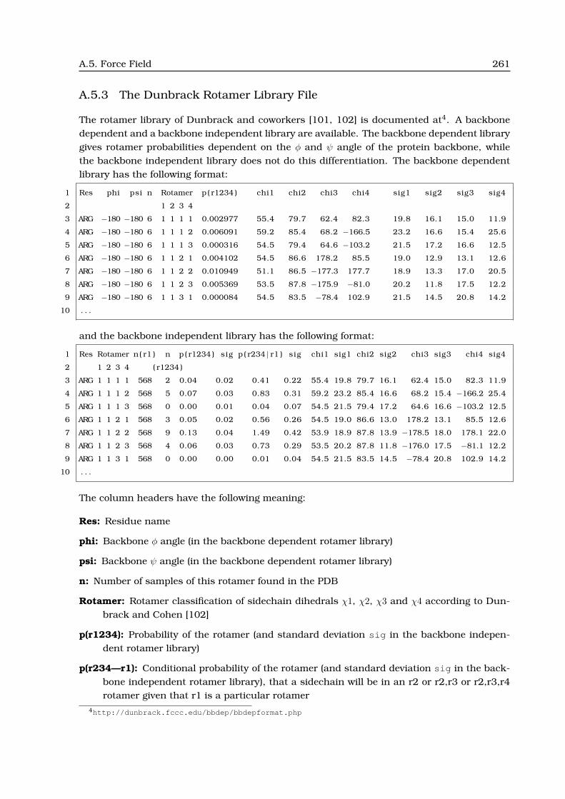
A.5. Force Field 261
A.5.3 The Dunbrack Rotamer Library File
The rotamer library of Dunbrack and coworkers [101, 102] is documented at4. A backbonedependent and a backbone independent library are available. The backbone dependent librarygives rotamer probabilities dependent on the φ and ψ angle of the protein backbone, whilethe backbone independent library does not do this differentiation. The backbone dependentlibrary has the following format:
1 Res phi psi n Rotamer p ( r1234 ) chi1 chi2 chi3 chi4 sig1 sig2 sig3 sig4
2 1 2 3 4
3 ARG −180 −180 6 1 1 1 1 0.002977 55.4 79.7 62.4 82.3 19.8 16.1 15.0 11.9
4 ARG −180 −180 6 1 1 1 2 0.006091 59.2 85.4 68.2 −166.5 23.2 16.6 15.4 25.6
5 ARG −180 −180 6 1 1 1 3 0.000316 54.5 79.4 64.6 −103.2 21.5 17.2 16.6 12.5
6 ARG −180 −180 6 1 1 2 1 0.004102 54.5 86.6 178.2 85.5 19.0 12.9 13.1 12.6
7 ARG −180 −180 6 1 1 2 2 0.010949 51.1 86.5 −177.3 177.7 18.9 13.3 17.0 20.5
8 ARG −180 −180 6 1 1 2 3 0.005369 53.5 87.8 −175.9 −81.0 20.2 11.8 17.5 12.2
9 ARG −180 −180 6 1 1 3 1 0.000084 54.5 83.5 −78.4 102.9 21.5 14.5 20.8 14.2
10 . . .
and the backbone independent library has the following format:
1 Res Rotamer n( r1 ) n p ( r1234 ) sig p ( r234 | r1 ) sig chi1 sig1 chi2 sig2 chi3 sig3 chi4 sig4
2 1 2 3 4 ( r1234 )
3 ARG 1 1 1 1 568 2 0.04 0.02 0.41 0.22 55.4 19.8 79.7 16.1 62.4 15.0 82.3 11.9
4 ARG 1 1 1 2 568 5 0.07 0.03 0.83 0.31 59.2 23.2 85.4 16.6 68.2 15.4 −166.2 25.4
5 ARG 1 1 1 3 568 0 0.00 0.01 0.04 0.07 54.5 21.5 79.4 17.2 64.6 16.6 −103.2 12.5
6 ARG 1 1 2 1 568 3 0.05 0.02 0.56 0.26 54.5 19.0 86.6 13.0 178.2 13.1 85.5 12.6
7 ARG 1 1 2 2 568 9 0.13 0.04 1.49 0.42 53.9 18.9 87.8 13.9 −178.5 18.0 178.1 22.0
8 ARG 1 1 2 3 568 4 0.06 0.03 0.73 0.29 53.5 20.2 87.8 11.8 −176.0 17.5 −81.1 12.2
9 ARG 1 1 3 1 568 0 0.00 0.00 0.01 0.04 54.5 21.5 83.5 14.5 −78.4 20.8 102.9 14.2
10 . . .
The column headers have the following meaning:
Res: Residue name
phi: Backbone φ angle (in the backbone dependent rotamer library)
psi: Backbone ψ angle (in the backbone dependent rotamer library)
n: Number of samples of this rotamer found in the PDB
Rotamer: Rotamer classification of sidechain dihedrals χ1, χ2, χ3 and χ4 according to Dun-brack and Cohen [102]
p(r1234): Probability of the rotamer (and standard deviation sig in the backbone indepen-dent rotamer library)
p(r234—r1): Conditional probability of the rotamer (and standard deviation sig in the back-bone independent rotamer library), that a sidechain will be in an r2 or r2,r3 or r2,r3,r4rotamer given that r1 is a particular rotamer
4http://dunbrack.fccc.edu/bbdep/bbdepformat.php

262 File Types and Formats
chi1 - chi4: Average sidechain dihedrals χ1, χ2, χ3 and χ4
sig1 - sig4: Standard deviation of sidechain dihedrals χ1, χ2, χ3 and χ4
A.5.4 The Bondi Radii File
The Bondi radii [147] are read from a file with the following format:
1 RAD FE 1.3
2 RAD MG 1.6
3 RAD CU 1.3
4 RAD N 1.55
5 RAD C 1.7
6 RAD O 1.5
7 RAD S 1.8
8 RAD H 1.2
9 RAD P 2.0
Each line starts with the keyword RAD followed by the name of the chemical element and theradius. Comments are prefixed with an exclamation mark.
A.6 The QMPB Input File
The input file of QMPB is described in section 4.3.3 based on examples. Here, a list of availablekeywords for each block is given for reference.
A.6.1 The General Block
Example:
1 meadpath = /home/essigke/bin
2 T = 300
3 I = 0.1
4 backfi le = background . pqr
5 MGMcenter = ON CENT OF INTR
6 MGMpoints = 131
7 MGMspace = 0.2
8 OGMcenter = ON GEOM CENT ON CENT OF INTR
9 OGMpoints = 131 131
10 OGMspace = 1 0.2
11 epsin1 = 1
12 epsin2 = 4
13 Ligand Labels = proton electron
meadpath: Path to the MEAD programs, i.e., Pqr2SolvAccVol, My 2Diel Solver and My 3Diel Sol-ver (mandatory).

A.6. The QMPB Input File 263
T: Temperature in Kelvin (mandatory).
I: Ionic strength in moll (mandatory).
backfile: Filename of the background pqr-file. The background pqr-file contains all atomswhich are not part of any site. It must not contain atoms, which are part of any site(mandatory).
MGMcenter: As many strings (ON ORIGIN, ON GEOM CENT or ON CENT OF INTR, see appendixA.3) as there are focussing steps. The values define the center of the model grid meshused for solving the PBE for a model compound (optional).
MGMpoints: As many uneven integer numbers as there are focussing steps. The values givethe number of grid points in the model grid mesh used for solving the PBE for a modelcompound (optional).
MGMspace: As many positive floating point numbers as there are focussing steps. The valuesgive the spacing between grid points in the model grid mesh used for solving the PBE fora model compound (optional).
OGMcenter: As many strings (ON ORIGIN, ON GEOM CENT or ON CENT OF INTR, see appendixA.3) as there are focussing steps. The values define the center of the object grid meshused for solving the PBE for a MMsite or QMsite (optional).
OGMpoints: As many uneven integer numbers as there are focussing steps. The values givethe number of grid points in the object grid mesh used for solving the PBE for a MMsite
or QMsite (optional).
OGMspace: As many positive floating point numbers as there are focussing steps. The valuesgive the spacing between grid points in the object grid mesh used for solving the PBE fora MMsite or QMsite (optional).
Ligand Labels: As many strings as there are ligand types. The strings are the ligand typelabels in the order of the N option in the other blocks (mandatory).
workdir: Name of the directory created by QMPB to write the job.sh script and all files neededto run the helper programs called by the script (optional, default qmpb).
epsin1: Dielectric constant of the region of atoms with quantum mechanically derived charges(mandatory, even if there are no atoms given for this dielectric region).
epsin2: Dielectric constant of the region of atoms with force field charges (mandatory).
A.6.2 An Instance of a QMsite
The block starts with a line
QMsite site label instance label
and ends with a line starting a block for another instance or with a keyword belonging tothe general block. The site label is a user defined tag for the site. Instances of the samesite must have the same site label, while different sites must have a different site label.

264 File Types and Formats
The site label may contain the residue name and number as well as a chain identifier. Theinstance label is a user defined tag for the instance of the site. Instances of the same sitemust have different instance labels.
Example:
1 QMsite s i te C PHE 39 A instance 0 ox
2 f i l e =s i te C PHE 39 Ainstance 0 ox . pqr
3 sid=21
4 i id=0
5 eps= 1
6 Hqm=−14998.1
7 Gvib=98.693
8 N= 0 0
9 Gfree= 0 −102.1558
10 QM corr C PHE 39 A. pqr int C PHE 39 A. pqr
11 QM corr O PHE 39 A. pqr int O PHE 39 A. pqr
12 . . .
Hqm: Energy of formation or total bonding energy, Hvac,i(jk), of the instance in the dielectriceps (mandatory).
Gvib: Vibrational energy, Gvib,i(jk), of the instance calculate by normal mode analysis (manda-tory).
Gfree: Array of energies of unbound ligands, Gfree,i(jk), for each ligand type λ. The length andorder has to be consistent with the Ligand Labels in the global block (mandatory).
Gcorr: Electrostatic correction energy, Gcorr,i(jk) (section 3.3.1), of the instance calculated ina previous run. It can not be used in combination with the QM corr keyword (optional).
QM corr: This option does not follow the general key=value pair syntax and unlike otheroptions is allowed to occur more than once in the block of an instance. The keywordis followed by two pqr-file names, the first containing an atom of the QMsite and thesecond containing all atoms outside the side, with which the atom is in a bond or anglerelationship. The PBE is solved for each line with the QM corr keyword to obtain a contri-bution to the correction energy, Gcorr,i(jk). For most QMsites calculating the correctionenergy is computationally very costly. Therefore, a once computed correction energy canbe given as input using the Gcorr keyword (optional).
file: Name of the pqr-file defining the coordinates and charges of atoms belonging to theinstance (mandatory).
eps: Dielectric constant of the region to which the instance belongs. Currently, it has to beidentical with either epsin1 or epsin2 in the general block (mandatory).
N: Array of numbers of bound ligand, nλ,i(jk), for each ligand type λ. The length and orderhas to be consistent with the Ligand Labels in the global block (mandatory).
OGMpoints, OGMspace, OGMcenter: The keywords have the same meaning as in the gen-eral block, but they define the grid for the site only. Therefore, the keywords can only be

A.6. The QMPB Input File 265
given for one instance of each site. By that, it is possible to calculate most sites with asmall grid as final focussing step (e.g., fitting to an amino acid sidechain), but to define alarger grid for a particular site (e.g., a heme), which is significantly larger than an averagesite (mandatory, if not defined in the general block).
center: If the string ON CENT OF INTR is used in the grid definition, the geometric center of allinstances of the site is calculated. Instead, it is possible to define a center coordinate,e.g., (0.0,0.0,0.0), once for a site (optional).
sid: Numerical site identifier required by some of the post-processing programs. The outputis sorted by numerical identifiers (unique for each site, optional).
iid: Numerical instance identifier required by some of the post-processing programs. The out-put is sorted by numerical identifiers (unique for a instance in a particular site, optional).
A.6.3 An Instance of a MMsite
The block starts with a line
MMsite site label instance label
and ends with a line starting a block for another instance or with a keyword belonging tothe general block. The site label is a user defined tag for the site. Instances of the samesite must have the same site label, while different sites must have a different site label.The site label may contain the residue name and number as well as a chain identifier. Theinstance label is a user defined tag for the instance of the site. Instances of the same sitemust have different instance labels.
Example;
1 MMsite s i te HT1 ALA 1 A instance 0 C
2 f i l e =s i te HT1 ALA 1 Ainstance 0 C. pqr
3 sid=0
4 i id=0
5 re f=se l f
6 eps= 4
7 N= 0 0
8 Gmm=0.3299
ref: Reference by instance label either pointing to a Modelsite or another rotamer of thesame site with identical N array. If the reference points to a Modelsite, the energy ofthe site is calculated relative to the model energy. If the reference points to a differentrotameric form, the energy is calculated relative to the energy of the other rotameric form.If the string self is used, the instance is a reference instance (section 3.4, mandatory).
Gmm: Rotamer energy, Grotamer(jk), of the instance. The term is used when calculating theenergy of an instance relative to another rotameric form of the same instance (manda-tory).
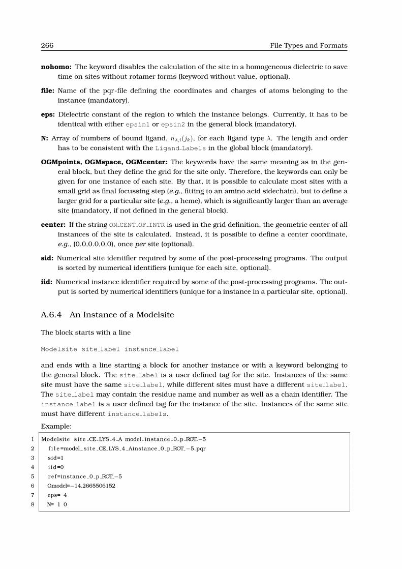
266 File Types and Formats
nohomo: The keyword disables the calculation of the site in a homogeneous dielectric to savetime on sites without rotamer forms (keyword without value, optional).
file: Name of the pqr-file defining the coordinates and charges of atoms belonging to theinstance (mandatory).
eps: Dielectric constant of the region to which the instance belongs. Currently, it has to beidentical with either epsin1 or epsin2 in the general block (mandatory).
N: Array of numbers of bound ligand, nλ,i(jk), for each ligand type λ. The length and orderhas to be consistent with the Ligand Labels in the global block (mandatory).
OGMpoints, OGMspace, OGMcenter: The keywords have the same meaning as in the gen-eral block, but they define the grid for the site only. Therefore, the keywords can only begiven for one instance of each site. By that, it is possible to calculate most sites with asmall grid as final focussing step (e.g., fitting to an amino acid sidechain), but to define alarger grid for a particular site (e.g., a heme), which is significantly larger than an averagesite (mandatory, if not defined in the general block).
center: If the string ON CENT OF INTR is used in the grid definition, the geometric center of allinstances of the site is calculated. Instead, it is possible to define a center coordinate,e.g., (0.0,0.0,0.0), once per site (optional).
sid: Numerical site identifier required by some of the post-processing programs. The outputis sorted by numerical identifiers (unique for each site, optional).
iid: Numerical instance identifier required by some of the post-processing programs. The out-put is sorted by numerical identifiers (unique for a instance in a particular site, optional).
A.6.4 An Instance of a Modelsite
The block starts with a line
Modelsite site label instance label
and ends with a line starting a block for another instance or with a keyword belonging tothe general block. The site label is a user defined tag for the site. Instances of the samesite must have the same site label, while different sites must have a different site label.The site label may contain the residue name and number as well as a chain identifier. Theinstance label is a user defined tag for the instance of the site. Instances of the same sitemust have different instance labels.
Example:
1 Modelsite s i t e CE LYS 4 A model instance 0 p ROT −5
2 f i l e =model s i t e CE LYS 4 Ainstance 0 p ROT −5.pqr
3 sid=1
4 i id=0
5 re f=instance 0 p ROT −5
6 Gmodel=−14.2665506152
7 eps= 4
8 N= 1 0

A.6. The QMPB Input File 267
ref: Reference by instance label pointing to the MMsite to which the Modelsite belongs(mandatory).
Gmodel: Energy of the model compound relative to a different instance of the same modelcompound, e.g., the user defines a instance as the reference form for the site and givesall experimental values relative to this instance.
file: Name of the pqr-file defining the coordinates and charges of atoms belonging to theinstance (mandatory).
eps: Dielectric constant of the region to which the instance belongs. Currently, it has to beidentical with either epsin1 or epsin2 in the general block (mandatory).
N: Array of numbers of bound ligand, nλ,i(jk), for each ligand type λ. The length and orderhas to be consistent with the Ligand Labels in the global block (mandatory).
MGMpoints, MGMspace, MGMcenter: The keywords have the same meaning as in the gen-eral block, but they define the grid for the site only. Therefore, the keywords can only begiven for one instance of each site. By that, it is possible to calculate most sites with asmall grid as final focussing step (e.g., fitting to an amino acid sidechain), but to define alarger grid for a particular site (e.g., a heme), which is significantly larger than an averagesite (mandatory, if not defined in the general block).
center: If the string ON CENT OF INTR is used in the grid definition, the geometric center of allinstances of the site is calculated. Instead, it is possible to define a center coordinate,e.g., (0.0,0.0,0.0), once per site (optional).
sid: Numerical site identifier required by some of the post-processing programs. The outputis sorted by numerical identifiers (unique for each site, optional).
iid: Numerical instance identifier required by some of the post-processing programs. The out-put is sorted by numerical identifiers (unique for a instance in a particular site, optional).

268 File Types and Formats

APPENDIX B
MANUAL PAGES
B.1 QMPB
Name
QMPB - Quantum Mechanics bases Poisson Boltzmann
Synopsis
qmpb.pl <qmpb.in> -b|-a [-gmct] [-inputorder] [-pf]
Description
QMPB calculates ligand binding energies of ligands of a macromolecule by a continuum elec-trostatic approach.
Reference reactions can be obtained by quantum mechanics in vacuum or measured for modelcompounds in solution. The transfer energy of the reactants and products from the referencereaction environment into the macromolecule is calculated by helper programs solving thelinearized Poisson-Boltzmann equation (LPBE). QMPB generates the input for the LPBE solversin a pre-processor mode (option -b) and condenses the output into a file of intrinsic energiesand a file of interaction energies in a post-processor mode (option -a). The program run islargely input file driven (<qmpb.in>), which is described in appendix A.6. Most of the work ofQMPB is performed by objects, which are defined in module files. If the module files are not inthe default Perl path, the path to the module files has to be given by setting the environmentvariable PERL5LIB appropriately.
Options
-a: Run in post-processor mode (after)
-b: Run in pre-processor mode (before)
269

270 Manual Pages
-gmct: Write output (in post-processor mode) in a format suited for reading by SMT and GMCT,i.e., site and instance identifiers start at one (optional). By default all counting in QMPBstarts with zero.
-inputorder: Read site identifiers sid and instance identifier iid from input file (optional).By default the output is given in the order of internally generated Perl hashes.
-pf: Calculate protein field energies by passing this option to My 3Diel Solver (optional). If theflag is set each coordinate and charge in the background pqr-file is copied to a fpt-file(protein.fpt), which is processed by My 3Diel Solver. The output is not analyzed byQMPB, but has to be handled by external programs.
Environment
PERL5LIB: Directory to search for Perl modules of QMPB (see man perlrun).

B.2. Pqr2SolvAccVol 271
B.2 Pqr2SolvAccVol
Name
Pqr2SolvAccVol - Calculate the analytical description of the ”Solvent Accessible Volume” froma pqr-file.
Synopsis
pqr2SolvAccVol [-solrad <value>] [-ascii] [-blab1|blab2|blab3] <molname>
Description
The program Pqr2SolvAccVol reads a extended pqr-file (<molname>.pqr) as input and writesthe analytical surface description of the solvent accessible volume(s) of the molecule(s) to anoutput file (<molname>.txt for ASCII format and <molname>.dat for binary format). Thesolvent accessible surface is calculated by a rolling probe (section 2.2.6) and described ana-lytically [70]. For complex molecules the calculation is time consuming and redundant for allMy 3Diel Solver calculations. Therefore, pre-calculating the surfaces reduces the overall com-putational time. It is fast to map the analytical surface representation to dielectric constantson a discrete grid for a particular focussing step.
Additionally, by reading always the same surfaces for dielectric regions it is ensured thatdielectric boundaries stay constant, even if the coordinates of some atoms change. ThereforeMy 3Diel Solver reads different files for calculating boundaries and electrostatic energies.
To ensure that all atoms of rotameric forms are inside their dielectric region, the pqr-file gen-erated by QMPB contains all instances of all sites. Therefore, for sites with different rotamericforms the dielectric region is larger as it would be if only the rotameric form of interest wouldbe included. The error is small if the rotamers are similar, i.e., if only hydrogen rotamers areincluded.
Internally, Pqr2SolvAccVol reads <molname>.pqr into an AtomSet object and a SolvAccVol
object is created from the AtomSet. All classes and invoked methods are part of the unmodi-fied MEAD library.
Options
-solrad: Set the probe radius (in A) for the probe, which will be rolled over the molecularsurface (default 1.4 A). A smaller radius will give deeper cusps between the atoms whilea larger radius will give a smoother surface. The default value is often used for water.
-ascii: Write the output in ASCII format. The default, binary format gives smaller files and isfaster to read by the MEAD programs, but is not human readable.
-blab*: The ”blab”-level determines the amount of debug output written to STDOUT. A highervalue increases the verbosity.

272 Manual Pages
B.3 My 3Diel Solver
Name
My 3Diel Solver - Solve the LPBE for an instance of a site in a three dielectric environment.
Synopsis
my 3diel solver -epsin1 <value> -epsin2 <value> [-epsext <value>]
[-epsvac <value>] [-solrad <value>] [-sterln <value>]
[-ionicstr <value>] [-T <value>] [-kBolt <value>]
[-conconv <value>] [-econv <value>]
[-bohr radius <value>] [-proton charge <value>]
[-converge oldway <value>] [-blab1|blab2|blab3]
[-eps1set <eps1set>] [-eps2set <eps2set>]
[-fpt <extended fpt-file>] [-pf <extended fpt-file>]
[-epshomo <value>] <instance> <background>
Description
The program My 3Diel Solver solves the linearized Poisson-Boltzmann equation (LPBE) in a(up to) three dielectric environment. Therefore it is compareable with Solinprot, however itmay not calculate a homogeneous transfer energy, but only a Born and a background energy.Grid artefacts may need to be canceled by an accompanied calculation of My 2Diel Solver. Itis used for computing electrostatic energies for instances of the QMsite and MMsite class inQMPB.
Options
Most options are defined in the documentation provided with the MEAD package. Here, onlynew options are explained.
-eps1set: Specifies a file <eps1set>.pqr containing all atoms in the region with dielectricconstant -epsin1. If a file <eps1set>.txt or <eps1set>.dat exists, it is read addi-tionally to the pqr-file, assuming that the file was generated by Pqr2SolvAccVol from thepqr-file. The file <eps1set>.dat is preferred for smaller file size and higher numeri-cal accuracy. Else the analytical surface representation is calculated using the radius-solrad. Finally, the pqr-file is used to calculate the ElectrolyteEnvironment.
-eps2set: Specifies a file <eps2set>.pqr containing all atoms in the region with dielectricconstant -epsin2. Analogously to the eps1set, analytical surface representations canbe read from file.
-fpt: Specifies an extended fpt-file to be read (appendix A.1.5). The electrostatic potential iscalculated at the given coordinates and multiplied by the given charges. The interactionenergy is summed up for each instance of each site and given in the output.

B.3. My 3Diel Solver 273
-pf: Specifies an extended fpt-file to be read (appendix A.1.5). The electrostatic potential iscalculated at the given coordinates and multiplied by the given charges. The electrostaticenergy is given in the output file marked by the string “PF-TAG”. This option, thought fordebugging or detailed analysis of background or interaction energy terms, is ignored byQMPB.
-epshomo: Additionally to the calculation in the three dielectric environment a calculation ina homogeneous environment can be done. The homogeneous dielectric is set to the givenvalue.

274 Manual Pages
B.4 My 2Diel Solver
Name
My 2Diel Solver - Solve the LPBE for a model compound of an instance of a site in a twodielectric environment.
Synopsis
my 2diel solver -epsin <value> [-epsext <value>] [-epsvac <value>]
[-solrad <value>] [-sterln <value>] [-ionicstr <value>]
[-T <value>] [-kBolt <value>] [-conconv <value>]
[-econv <value>] [-bohr radius <value>]
[-proton charge <value>] [-converge oldway <value>]
[-blab1|blab2|blab3]
<instance> <model-background>
Description
The program My 2Diel Solver solves the linearized Poisson-Boltzmann equation (LPBE) in atwo dielectric environment. Therefore it is compareable with Solvate, however it does notcalculate a homogeneous transfer energy, but only a Born and a background energy. Gridartefacts have to be canceled by an accompanied calculation with My 3Diel Solver. It is usedfor computing electrostatic energies for model compounds of instances of sites of the MMsite
class in QMPB.
While Solvate reads one pqr-file, which is used for both, calculating the dielectric bound-aries and the electrostatic energies, My 2Diel Solvertakes two extended pqr-files. The file<instance>.pqr contains the coordinates and charges of the instance. It is identical withthe file used in the associated My 3Diel Solver calculation. The file <model-background>.pqrcontains all atoms of the model compound defining the dielectric boundary between the tworegions with dielectric constant -epsin and -epsext. Charges belonging to atoms of the in-stance of the site must be set to zero, while charges of other atoms define the backgroundcharge set of the model compound. The file <model-background>.pqr is also used to calcu-late the ElectrolyteEnvironment.
Pre-calculating surfaces as in My 3Diel Solver was not found to be useful, because each aminoacid of the same type is probably in a different reference rotamer. Also some effort would benecessary to rotate and translate the surface of one site onto the coordinates of another.
Options
All options are defined in the documentation provided with the MEAD package.

B.5. Multiflex2qmpb 275
B.5 Multiflex2qmpb
Name
Multiflex2qmpb - Convert Multiflex input into an input file for QMPB.
Synopsis
multiflex2qmpb.pl <molname> > qmpb.in
Description
The program Multiflex2qmpb converts input files written for Multiflex into an input file forQMPB. Only a subset of QMPBs options are available: Only relative ligand binding energies ofsites without rotamers1 can be calculated. Unlike Multiflex, Multiflex2qmpb can handle est-files of sitetype MMsite additionally to st-files. Therefore, it is possible to perform calculationswith more than two charge forms and different ligand types.
The program expects the files <molname>.pqr (appendix A.1.2 or appendix A.1.3), <mol-
name>.sites (appendix 3.3), <molname>.ogm and <molname>.mgm (appendix A.3). For eachresidue name given in the file <molname>.sites, a st-file or est-file is expected. st-files(appendix A.2.1) are assumed to contain charge sets for proton binding and energies givenin pKa-units for compatibility with Multiflex. The est-file is documented in appendix A.2.2. Iffiles of both types are present, the est-file is preferred. Residues with more than one tautomer(histidine, N- and C-terminus of residues with titrateable sidechain) have to be given in anest-file instead using two (or more) st-files as in Multiflex.
The pqr-file of the model compound is generated by taking the whole residue (not just theatoms given in the st-file or est-file) and additional atoms of the previous and next residuespecified in the arrays prev res and next res inside the Multiflex2qmpb sourcecode. Theseatoms are expected to change rarely and are also hardcoded in Multiflex. Also the defaultparameters are adjustable in the Perl source code.
Absolute ligand binding energy calculations are not supported by Multiflex2qmpb and have tobe added by modifying the QMPB input file qmpb.in.
To be compatible with Multiflex, multiple st-files can be specified per residue. Each chargecolumn in the st-file has to have integer charge. One column has to have a charge sum ofzero, because the uncharged form is chosen as reference form. All atoms which are mentionedin any st-file given for the residue are set to one of the charge forms from the st-fileThe chargesin the pqr-file are ignored.
Environment
PERL5LIB: Directory to search for Perl modules of Multiflex2qmpb (see man perlrun).
MEADPATH: $MEADPATH/bin is the value of the QMPB option meadpath (see appendix A.6).
1Simple rotamers can be included as charge forms.

276

Hiermit erklare ich, dass ich die vorliegende Arbeit selbstandigverfasst und keine anderen als die von mir angegebenenQuellen und Hilfsmittel verwendet habe.
Ferner erklare ich, dass ich anderweitig mit oder ohne Erfolgnicht versucht habe, diese Dissertation einzureichen. Ich habekeine gleichartige Doktorprufung an einer anderen Hochschuleendgultig nicht bestanden.
Timm Essigke
Bayreuth, den 20. Dezember 2007