RADIAL FLOW BETWEEN TWO PARALLEL DISCS

by

RONO TSU YEN

B. S., National Taiwan University, I962

submitted in partial ftilfiUment of the

requirements for the degree

MASTER OF SCIENCE

Department of Applied Mechanics

KANSAS STATE UNIVERSITTManhattan, Kansas

A MASTER'S REPORT

1965

Approved by:

brought to you by COREView metadata, citation and similar papers at core.ac.uk

provided by K-State Research Exchange

C, X ,TABLE OF CONTENTS

INTRODUCTION 1

THEORETICAL ANALYSIS 3

RESULTS 1^

DISCUSSION OF RESULTS 21

RECOM-SNDATIONS FOR FUTURE STUDT 22

ACKNOWLSDGEI^iENT • 23

BIBLIOGRAFHT ' 2^

INTRODUCTION

The laminar flow of a viscous fluid between two infinite parallel

plates, provided the flow remains laminar, is termed a Poiseuille flow

for idiich an exact solution for flow characteristics may be obtained. In

a laminar flow, all fluid elements move in ordered parallel layers, neither

crossing one another's path nor mixing with one another. A thin layer of

real fluid adheres to the solid walls of the plates therefore the velocity

all along the wall is zero. It is reasonable to assume that the velocity

distribution at any cross section is symmetrical about the center line,

so that all points equi-distant from the plates have the same velocity.

The radial flow between two parallel discs of ideal fluid takes place

because of a pressure drop AP between the inner and outer radii r^^ and Tg,

and represents a simple elementary inviscid flow.

It is the purpose of this report to study the laminar flow of a

viscous fluid between two infinite parallel discs, as in Figure 1, as an

extension of the two previous problems.

Flow in

Figure 1

Such a flow could represent, in an idealized, form, an exaB^xLe, a thrust

bearing \ixosQ proper design wuld require knowledge and study of the hydro-

2

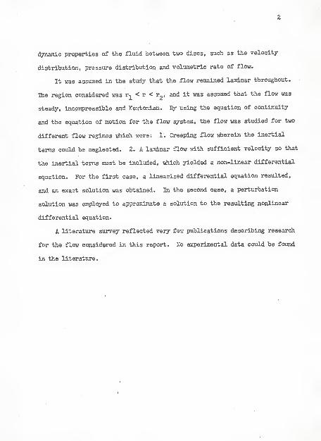
dynamic properties of the fluid between two discs, such as the velocity

distribution, pressure distribution and volumetric rate of flow.

It was assumed in the study that the flow remained laminar throughout.

The region considered was r^^ < r < r2. and it was assmned that the flow was

steady, incompressible and Newtonian, using the equation of continuity

and the equation of motion for the flow system, the flow was studied for two

different flow regimes viiich were: 1. Creeping flow \dierein the inertial

terms could be neglected. 2. A laminar flow with sufficient velocity so that

the inertial terms must be included, vAich yielded a non-linear differential

equation. For the first case, a linearized differential equation resulted,

and an exact solution was obtained. In the second case, a perturbation

solution was employed to approximate a solution to the resulting nonlinear

differential equation.

A literature survey reflected very few publications describing research

for the flow considered in this report. No experimental data could be found

in the literature.

3

THEORETICAL ANiOXSIS

In the analysis that flows, the following notation will be used:

r = radius to any point, feet

= inner radius, feet

r^ = outer radius, feet

V = radial component of velocity, feet/secondr

Vq = pheripherical component of velocity, feet/second

V = z-component of velocity, feet/second

p = density, slugs/feet-^

P = pressure, pounds/feet^

= pressure at r^, pounds/feet^

H = absolute viscosity, pound-second/feet^

Q = volumetric flow, cubic feet/second

T)f

ratio of depth

C, 0^^,02 = integration constants

D _ b^ AP'

liln rg/r^

\ p(Xlv^ ' Ih^) b^

Assume that a radial flow between parallel discs is steady, laminar,

incompressible, Newtonian, and consider the region ^

From Navier Stokes equations

'r Sr " r * az p Sr pP ^TT r a?" " ~ TT^

The flow is assumed to be radial then Vq = 0, and = 0; and the flow

produced by a pressure difference between the inner and outer radius.

Since Va = V =0, Equation (1) reduces too Z

-1^=0 or f =p dz CLZ

liiich implies pressure is independent of z, hence pressure is ftmction of r

only.

Bie continuity equation for the flow described is

r ^._r + z ^Br r oz

but since »

T-^ + — =ar r

Differentiation with respect to r yields

A(!!r^!r),f!r^l!!r3«oar ^ar * r ^ ^^2 ^ r ar ^.2

' "

Substitution into Equation (1) yields

V = + (3)V ar p ar *p

but since

ar

thea

5

]QitegratiQn of this expression yields

In r = - In Vj» + In $(z)

or

r r

>4iere $(z) is the constant of integration.

If the above expression for is substituted into Equation (2), one

obtains

r^Cz) > „ . 1 dP . t $"(z)r ^ ^2 ' p dr p r

or

H$"(z)^+i!Mdr = idPP r jJ3 P

liiich may be integrated with respect to r

to yield the above non-linear differential equation.

If the flow is creeping flow, fluid inertia is gmflii as compared to the

viscous shear, so that the inertial term may be neglected.

When the non-linear term is omitted, the resulting equation is

H In ^ i\z) « - AP'^l

or

6

In —

Integration with respect to z yields

* I / \ 1 . .

and a second integration gives

Hz)AP 1 2

2li r

Boundary conditions are, at z = + b the velocity is zero, so $(z) s

is satisfied and the coefficient = and » ^

and

2H In —'l

2r^ln-^

Figure 3

7

the rate of flow, Q. is then

Q « 2 r Y*2TTr dz

2r^l^^

4nb^ AP

In —^1

^ (1 - TlVn ,

^2

Finally since

th«n

AP « —

^

Perturbation Solution

A laminar flow with sufficient velocity so that the inertial term must*

be included gives rise to a non-linear differential equation. Saaty (2)* has

indicated that the principle of superposing solutions to obtain the general

solution of such a ^stem does not apply, as it does with a linear system.

* Bracketed numbers refer to corresponding reference in the bibliography.

8

As it is usually not possible to write down the general solution of such a

non-linear system, or even to obtain an exact particular solution, one

frequently resorts to careful approximations \iiose analysis reveals the

characteristic properties of the system containing a parameter e (introduced

for convenimce). The parameter e is a constant \^ose value will be set

anyi^ere between and 1. Its purpose is to control the size or magnitude

of the perturbation. As the perturbation is increased from to its full

value it is customary to suppose that the values of will vary in some

smooth manner from their starting point i^. There is no reason to expect

to deviate in an exactly liiiear manner from the "starting point" i^.

We must allow for some curvature. As in Figure 3 we approxinate the true

curve with a linear term e with a coefficient plus a second degree tern

2 2in c i&ich has different - and here smaller - coefficient i ,

Figure 3

9

If the curvature is sharper it may be necessary to synthesize the true

curve with terms dependent upon e^, e^, etc. tfe shall be concerned here

only with "first order" appraximations. Ihis means that we shall restrict

ourselves to perturbation in lAich, even \4ien the perturbation is "on" at

full density (e » 1), the square terms are in all cases small »4ien compared

idth the linear terms*

By introducing a parameter e, the non-linear equation may be written

1 « a2, w 1 1 N

'^l '^l

it is assumed that, for e ^

- *o(Tl) + ««l(l)) + «%(^) + ••• .<5)

idiere

^ = f

substitution of the two series (5)« (6) into Equation (4) and letting

1 « k2 , 1 1 >5Pb (-5--^)« b^ AP * ^ ^1 ^2

^2 ^2

^1 ^1

one obtains

L*"q(T1) +pJ

+ e [$\(T1) + B^Q^Cn)] + + 2B$o(Tl)*3^(Tl) + ...j «

Equating coefficients of like powers of e yields

«"q(T1)+P«0 (7)'

$\(n) + B$/(T1) =0

i\(T\) + 2B$q(11) $3^(11) «

These differential eqiuitions may be solved as follows

1. «"q(T1)--P- $'q=-P71 + Ci

to = -I PTl + +

Boundary conditions

H-i $0 = Cg-ip

«o«=|^^i-^'>

2- «\(T1) » - B$o^(Tl)

« -I

p2 (1 - 21)2 + Tl^)

= -I (| 1^ -

I +^ 11^) + +

Boundary conditions

T| « 1 «^(T]) =

T) = - 1 $3^(11) -.

°=-f^(|-|+#*Cl*<^2

= -Bp2(l.l^l.).C,+C2

11

* 30 2 6 30

- 55" *55^ >

«2(11) - - 1^ - lis H'* +^ -^ +5^ 1^")

Boundaxy conditions

11 - 1 *2(T)) =

T) = - 1 $2^^^ = <^

Ihe solution of $(z) may be expressed as'

Taking the perturbation at full density ( « > 1} then $(z) becomes

The expression for V^Cr.a) is then

V (r.z) ,^= I [$o(T)) + ^iC'H) + igCn) +

]

The volumetric rate of flow, Q, vill be given by

Q . 2nr.b ^ dT)

1» 2nb $q(T]) + $^(11) + $2(11) + ... dTI

*0(D) dH «I

P (1 - f) dH

-|x2P(l.iTl3)J«|p

J^*^(ll)d^»2.r^fp2(n.l^2^1^.^^j^^

" ^30 - 5 + 30 - 215^

. 1 «,8 1 JLO.

13

At last then,

2B^p3 , 4919 11 . 13 1^^TOOxTTf - 60 X 3 180 X 5 " ^Tx?

2B^P- 2 X 1048* 51975

3A

RESULTS

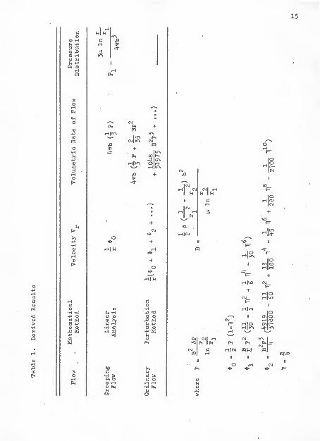
The following. Table 1, gives the results that were obtained from

the analysis. In the perturbation solution, the first term corresponds

to the creeping flow. Ihe higher terms account for the deviations from

creeping flow Tiien AP is increased. Since the deviation of the curve

is not great, only second degree terms were retained.

To illustrate the differences that might result from utilization of

each of the derived results, solutions were obtained for the following

assumed numerical data for the linearized as well as the nonlinear case.

The data used are as in Table 2. In Tables 3t ^» and 5 soce tabulated

the calculated quantities indicated, w^iile Table 6 gives the results for

creeping flow. Figure ^ and Figure 5 display the results graphically.

15

C\JI^

O

at CD

fi

t! >Pi OO rH0) Pm

cd O

o

CM1-41 CM

I ^

I

+

fH CO

I

i-||H

+

CM

r-l|0h|vo

CMl rH CM

(3 rH|CM PPM"

» I

O rH

16

Table 2. Assuzned Namerlcal Data

1^/1 1 Sy,2

, ^2 „ AP „ '^l ^2la?- P P» =- B« J

0.01' ^' 1* 2 X 10"5 1.388 0.985 0.036 AP 0.0266

lb-sec lb-sec^

1^ 1^

Table 3. Data of Volumetric Flow

P P « 0.036 AP o/^Tib B ^5 Q*/^

1 -Ife. Q^Q^ Q^Qj2 0.0266 f # 0.012.000ft.

2-^ 0,072 0.02^^ 0.0266 0.000007 #0 0.2«»-,007

ft."^

5 0.18 0.03 0.0266 0.000025 « 0.060,025ft.2

•

10 0.36 0.12 0.0266 0.0001 i 0.120,100ft.''

17

Table Perturbation Solution Calculation

11 « 11 = ±J

1 - 1 0.93 0.75 0.437

1130

" 1^ 0.3666 0.3353 0.252 0.1326

375c

1 ^6 . 1 -80.1301

1 TilO" 2755 '

0.12^ 0.0906 0.0498

Table 5. Perturbation Solution Velocity Profile

$0 « |p(l-Tf ) « 5„bVa?i?

2 "37800 ?0 " 180*

1 4.1 ^8 1 JLO.55^ - 2755^ >

0.018 0.000008 X 0.3666

^

0.18 X 0.93» 0.016?^

0.000008 X 0.3353

#

±10.018 X 0.75= 0.0135

0.000008 X 0.252

#0

0,018 :? 0.^375= 0.007875

0.000008 X 0.1326

7

18

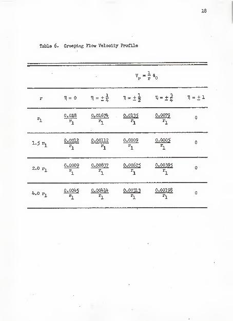
Table 6. Creepljig Flow Velocity Profile

^*0

r 1) = n = ±J1

Tl = ±| 11 « + 1

•L

0.018

'l

0.01674

^1

0.0135^"1

0.0079*•*^1

1.50.0012

1

0.00112r.1

0.0009

1

0.0005r_1

2.00.0009 0.00837 0.00625 0.00395

^1 ^1 ^1'^l

4.00.0045

^1

0.00414

^1

0.00313

'•l

0.00198

/l

20

^>^/o '

DISCUSSION OF RESULTS

Consideration of the numerical data shown in Figure k indicates that

between the linearized and perturbation solution, the deviation is very small,

and further, that the deviation appeared to be linear. Because of the small

deviation it would appear, at least for the range of pressure studied, that

the effect of the nonlinear term may be neglected. Figure 5 shows the velocity

profile for several different radii. No variation from the profile shown,

idiich are for the linear case, could be found if the nonlinear effects were

included.

22

RECOMMENDATIONS FOR FDTORE STDDI

In the prc)blem solved in this report it was assumed that the flow was

steady, incompressible, and Newtonian, and the flow was considered only for

the region r^ < r < rgt r^^ being the radius lAere the flow became fully

developed laminar flow. Thdse areas therein future study should be done

include: 1. an experimental study to determine the inlet distance required

to produce a fully developed laminar flow. 2. a study to determine the

Reynold's number for transition. 3» experimental verification of the velocity

profiles and pressure distribution. 4. extension of the analysis to include

non-Newtonian fluids and turbulent flow.

ACKNOWLEDGEMENT

I vLah to take this opportunity to express ny deep appreciation to

Professor John E. Kipp for his many helpful suggestions. His aid has been

instrumental in correcting and improTing this report*

BIBLIOGRAPHr

1. Bird, R. Byron, Warren E. Stewart, and Edwin N. lightfoot, "Transport

Phenomena," John Wll^ and Sons, Inc., I960,' p. 114. p. 122.

2. Saaty, Biomas L., and Joseph Bram, "Nonlinear Mathematics," McGraw-Hill

Book Company, 1964, p. 199-203.

3. Sherwin, Chalmers W., "Introduction to Quantumn Mechanics" Holt, Rinehart

and Winston, Inc., I960, p. 164-174.

4. Kauftaann, \falter, "Fluid Mechanics." McGraw-Hill Bode Company, 1963.

5. Eskionazi, Salamon, "Principles of Fluid Mechanics," Ally and Bacon, Inc.

p. 25.

RADIAL FLOW BETWEEN TWO PARALLEL DISCS

by

RONG TSU IM

B. S«, Hatlonal Taiwan Unlversl^t 1962

AH ABSTRACT OF A MASTER'S REPORT

sutoltted in partial fulflllmeat of the

requlrenents for the degree

MASTER OF SCIENCE

DepartniGQt of Applied )fechanl08

KANSAS STATE UNITERSITTManhattan, Kansas

1965

Radial, incompressible, Newtonian flov between two parallel discs Is

considered for a region r^ < r < rg ^iiereln the flow Is fully developed and

laminar. Expressions for the rate of flow, pressure distribution, and

velocity profile are presented. The analysis includes a study of creeping

flow, as well as an attempt to approximate the solution t6 nonlinear problem

by a pertuAation technique. Areas for future research are identified.