Optimization of Radial Impeller Geometry - CiteSeerX

RTO-EN-AVT-143 13 - 1

Optimization of Radial Impeller Geometry

R.A. Van den Braembussche von Karman Institute for Fluid Dynamics

72, Chaussée de Waterloo 1640 Rhode-Saint-Genèse

BELGIUM

[email protected]

ABSTRACT This lecture first provides an overview of the relation between the flow mechanisms in radial impellers and the 3D geometry. Special emphasis is given to secondary flows and the pressure gradients that govern them. It is followed by the description of a computerized optimization technique for the design of radial impellers. It is shown how the use of a Database, Artificial Neural Network and Genetic algorithm can be used to accelerate the design process and to improve performance.

INTRODUCTION The main advantage of Navier Stokes calculations is the availability of detailed information of the flow in a large number of locations. This allows the designer to base his judgment and modifications of the geometry on quantities that are directly related to that geometry. In this way it is much easier to define what changes are needed to improve the flow and as a consequence the performances. However too much information is given in too many locations and no indication is given on what geometrical changes will improve the performance. Hence this approach requires a good understanding of the relations between geometry and flow to foresee the impact of geometry changes on flow. One may also use numerical techniques to make more efficient use of them. Both approaches are discussed in the two following chapters.

The purpose of a first chapter is to provide a better insight into this relation, based on theoretical considerations and on the results of a parametric study. It is an attempt to provide a qualitative explanation of the various contributions to the three dimensional flow structure inside a turbomachine blade row.

The second chapter describes the VKI impeller optimization method, based on Artificial Neural Networks, Genetic Algorithm and 3D Navier Stokes solver, and its application to 3D radial impeller design. It includes multipoint and multidisciplinary optimization considerations.

1.0 FLOW STRUCTURE

1.1 The Meridional Balance of Forces

Neglecting the forces due to the blade lean (assuming .0=∂

∂n

bladeθ ), only two components of the absolute

velocity induce centrifugal accelerations in the meridional plane:

• The tangential component uV ( RWV uu Ω−= ) and

• The meridional velocity mV .

Van den Braembussche, R.A. (2006) Optimization of Radial Impeller Geometry. In Design and Analysis of High Speed Pumps (pp. 13-1 – 13-28). Educational Notes RTO-EN-AVT-143, Paper 13. Neuilly-sur-Seine, France: RTO. Available from: http://www.rto.nato.int/abstracts.asp.

http://www.rto.nato.int/abstracts.asp

mailto:[email protected]


13 - 2 RTO-EN-AVT-143

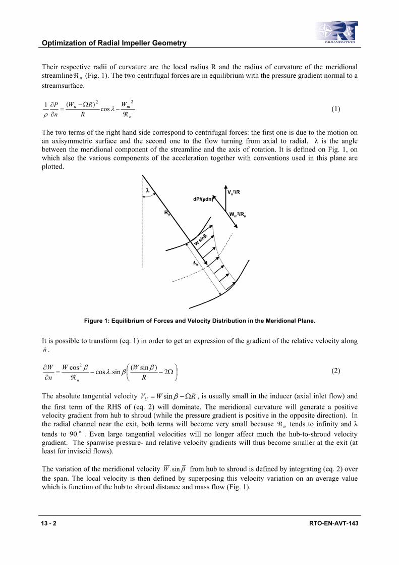
Their respective radii of curvature are the local radius R and the radius of curvature of the meridional streamline nℜ (Fig. 1). The two centrifugal forces are in equilibrium with the pressure gradient normal to a streamsurface.

n

mu WR

RWnP

ℜ−

Ω−=

∂∂ 22

cos)(1 λ

ρ (1)

The two terms of the right hand side correspond to centrifugal forces: the first one is due to the motion on an axisymmetric surface and the second one to the flow turning from axial to radial. λ is the angle between the meridional component of the streamline and the axis of rotation. It is defined on Fig. 1, on which also the various components of the acceleration together with conventions used in this plane are plotted.

Figure 1: Equilibrium of Forces and Velocity Distribution in the Meridional Plane.

It is possible to transform (eq. 1) in order to get an expression of the gradient of the relative velocity along n .

Ω−−

ℜ=

∂∂ 2)sin(sin.coscos2

RWW

nW

n

ββλβ (2)

The absolute tangential velocity RWVU Ω−= βsin , is usually small in the inducer (axial inlet flow) and the first term of the RHS of (eq. 2) will dominate. The meridional curvature will generate a positive velocity gradient from hub to shroud (while the pressure gradient is positive in the opposite direction). In the radial channel near the exit, both terms will become very small because nℜ tends to infinity and λ tends to 90.o . Even large tangential velocities will no longer affect much the hub-to-shroud velocity gradient. The spanwise pressure- and relative velocity gradients will thus become smaller at the exit (at least for inviscid flows).

The variation of the meridional velocity βsin.W from hub to shroud is defined by integrating (eq. 2) over the span. The local velocity is then defined by superposing this velocity variation on an average value which is function of the hub to shroud distance and mass flow (Fig. 1).


RTO-EN-AVT-143 13 - 3

∫∆

=n

dnWRm0

.cos....2 βπ (3)

Hence the hub to shroud velocity difference can be controlled in two ways:

• By changing the curvature radius of the meridional contour. Smaller curvature radii increase this hub to shroud velocity difference and can even result in negative velocities on the hub contour (Fig. 1). The opposite occurs when increasing the curvature radius (less curved meridional contour). Changing the curvature radius does not change the average velocity.

• By decreasing the distance between hub and shroud so that the same velocity gradient has to be integrated over a smaller length. At the same time the average velocity increases which helps to avoid return flow on the hub contour but increases the velocity on the shroud which is often not recommended from the point of view of cavitation.

Contrarily to an axial machine, where there is no meridional curvature force, it is possible in a radial machine to use the meridional curvature in order to decrease the spanwise pressure gradient resulting from the peripheral centrifugal force [1]. Fig. 2 illustrates it.

Figure 2: Zero Normal Pressure Gradient Design.

Imposing .0==∂∂

nP in the (eq. 1), one obtains:

λcos22

RVW u

n

m =ℜ

(4)

This equation defines the meridional curvature radius necessary for a zero pressure gradient from hub to shroud at all positions between impeller inlet and outlet.

However it can only be satisfied for one velocity between pressure and suction side. If one chooses to satisfy the relation (eq. 4) for the flow near the pressure side, where mV is small and uV is large, the corresponding radius of curvature should be very small. Inversely, if the relation (eq. 4) is satisfied near the suction side, where mV is large and uV is smaller, the radius of curvature should be large and the channel should be longer in the axial direction. This is illustrated on Fig. 3, where the influence of the number of blades is enlightened : if Z is large, the inter-blade distance is small and the velocity differences


13 - 4 RTO-EN-AVT-143

between both sides are also small. Hence the radii of curvature that satisfy the relation (eq. 4) do not vary much from pressure to suction side. This difference increases with decreasing blade number Z and the "optimal" meridional shapes become very different for pressure and suction sides. It is therefore not possible to define a meridional curvature that annuls the spanwise pressure gradient on both sides of the blade.

Figure 3: Influence of the Blade Number for Zero Pressure Gradient Design at Pressure and Suction Side (left: 48 blades, right: 24 blades).

If the meridional channel is optimized for the mid-pitch flow, the relation (eq. 4) will not be satisfied in the pressure and suction side boundary layers, where the same spanwise pressure gradient applies, but where mV goes to zero and uV goes to U. The centrifugal force will dominate over the curvature effects and the boundary layer fluid will be centrifuged towards the shroud. Although it is clear that the pressure gradient cannot be zero everywhere and that the three dimensional effects cannot be avoided, they can be minimized:

• By designing the meridional shape in function of the mean velocity variation to obtain a more uniform outlet flow; and

• By using a high number of blades in those regions where the pressure and suction side streamlines begin to diverge (use of splitters).

Other 3D inviscid effects that can not be taken into account by quasi-3D methods are tip leakage flow and blade lean.

1.2 Blade Lean Lean is the angle measured in spanwise direction between the blade and the hub or shroud surface. The angle can be constant along the span (straight lean) or can change along the blade height (compound lean) Fig. 4. Conventionally the lean is positive when the angle between the blade suction side and the hub is obtuse (>90.o). Introducing blade lean can influence the hub-shroud pressure gradient and impose a pressure gradient along the blades that is different from the one discussed in 1.1. The main consequence of lean is a redistribution of the flow in the spanwise direction influencing the impeller outlet velocity distribution and secondary flows. The lean angle between the blades and the hub at trailing edge is often called rake.


RTO-EN-AVT-143 13 - 5

Figure 4: Straight and Compound Lean.

The influence of lean on the pressure gradient is illustrated on Fig. 5 and 6. The meridional curvature and centrifugal forces create a hub to shroud pressure gradient defined by (eq. 2). It is schematically shown on Fig. 5a. Higher pressure regions are indicated with a + sign, low pressure regions have a - sign. Blade to blade pressure gradient is not introduced yet.

a

b

c

Figure 5: Pressure Distribution in a Crosswise Plane with Zero Lean.

The blade to blade loading in the circumferential direction increases the pressure on the pressure side and lowers it on the suction side as shown on Fig. 5b. The hub to shroud pressure gradient is assumed to be zero.

Combining the two pressure gradients provides a pressure field with iso-pressure lines shown on Fig. 5c. The highest pressure occurs in the hub pressure side corner and the lowest one in the shroud suction side corner.

Repeating the same exercise on a cross section with positive lean results in the pressure distributions shown on Fig. 6. The hub to shroud pressure gradient, based on the average blade to blade velocity, is almost unchanged (Fig. 6a). The assumption of axisymmetric flow does not account for the circumferential shift of the blades between hub and shroud. The blade to blade pressure distribution is changed because there is no mechanism to support a pressure gradient in the spanwise direction (fig. 6b). The hub to shroud pressure gradient perpendicular to the hub wall is still zero but the average hub pressure is increased and the average shroud pressure is decreased. The combined pressure field shows a much


13 - 6 RTO-EN-AVT-143

larger pressure at the hub pressure side corner and a decrease of pressure near the shroud suction side Fig. 6c). The result is a force pushing the fluid away from the hub and an increase of the through flow velocity near the shroud. A discussion on the impact of lean on secondary flow comes later.

a

b c

Figure 6: Influence of the Blade Lean on the Pressure Distribution in a Crosswise Plane.

The hub to shroud pressure gradient resulting from lean is relatively small and maybe negligible in areas where the hub to shroud pressure gradient, defined by (eq. 1), is dominant. In case the hub to shroud pressure gradient is small, because o.90=λ and the curvature nℜ ∞≈ , as in low specific speed impellers, the lean may have a stronger effect.

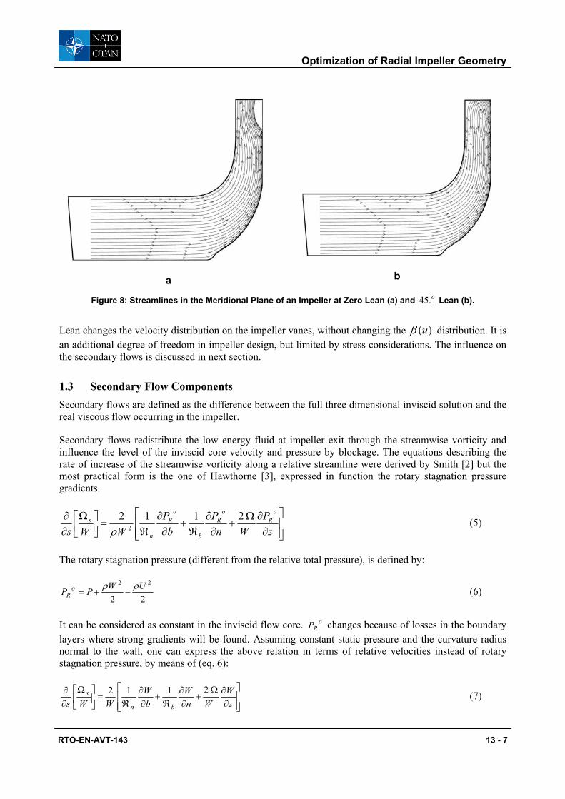
Fig. 7 clearly shows the change of impeller exit radial velocity distribution when introducing 45.o rake at the trailing edge. It turns out that lean is a powerful mean to redistribute the velocity at the impeller exit and to avoid separation and local return flow in the diffuser. This is illustrated on Fig. 8 for a low specific speed impeller. The effect might be smaller on a high specific speed impeller. It could however be enhanced by reducing the hub to shroud pressure gradient due to the meridional curvature.

Figure 7: Radial Velocity and Flow Angle at Impeller Exit With and Without Lean.


RTO-EN-AVT-143 13 - 7

a

b

Figure 8: Streamlines in the Meridional Plane of an Impeller at Zero Lean (a) and o.45 Lean (b).

Lean changes the velocity distribution on the impeller vanes, without changing the )(uβ distribution. It is an additional degree of freedom in impeller design, but limited by stress considerations. The influence on the secondary flows is discussed in next section.

1.3 Secondary Flow Components Secondary flows are defined as the difference between the full three dimensional inviscid solution and the real viscous flow occurring in the impeller.

Secondary flows redistribute the low energy fluid at impeller exit through the streamwise vorticity and influence the level of the inviscid core velocity and pressure by blockage. The equations describing the rate of increase of the streamwise vorticity along a relative streamline were derived by Smith [2] but the most practical form is the one of Hawthorne [3], expressed in function the rotary stagnation pressure gradients.

∂∂Ω

+∂∂

ℜ+

∂∂

ℜ=

Ω

∂∂

zP

WnP

bP

WWs

oR

oR

b

oR

n

s 21122ρ

(5)

The rotary stagnation pressure (different from the relative total pressure), is defined by:

22

22 UWPP oR

ρρ−+= (6)

It can be considered as constant in the inviscid flow core. oRP changes because of losses in the boundary

layers where strong gradients will be found. Assuming constant static pressure and the curvature radius normal to the wall, one can express the above relation in terms of relative velocities instead of rotary stagnation pressure, by means of (eq. 6):

∂∂Ω

+∂∂

ℜ+

∂∂

ℜ=

Ω∂∂

zW

WnW

bW

WWs bn

s 2112 (7)


13 - 8 RTO-EN-AVT-143

The first two right hand side terms express the generation of vorticity due to the flow turning, respectively in the meridional plane and in the blade-to-blade plane. The last term has its origin in the Coriolis forces and will thus occur only in the radial part of the impeller. The second and third terms will generate so-called passage vortices (PV) because they drive low energy fluid from the pressure towards the suction surface along the hub and shroud endwalls. The first term, due to the meridional curvature, will generate vortices along the blade surfaces (BV) from hub to shroud. Fig. 9 illustrates schematically these different vortices.

a

b

c

Figure 9: Definition of Individual Vortices.

The following comments about the three terms of this expression can be made:

• The passage vortices (PV), due to the flow turning in the blade to blade plane (second of RHS terms) (Fig. 9.a), will usually be stronger in the first half of the impeller channel, because the radius of curvature bℜ of the blade decreases when the local radius R increases. The passage vortex also starts from the leading edge because the hub and shroud boundary layer already exist.

Moreover, the relative velocity W being higher near the shroud than at the hub, the gradients nW∂∂

will be stronger at the shroud, where stronger passage vortices are thus expected.

• The blade surface vortices (BV), generated by the meridional curvature (first of the RHS terms) (Fig. 9b), will develop in the axial-to-radial elbow of the channel and will then vanish progressively in the radial channel. As the radius of curvature is smaller at the shroud, the rate of creation of these vortices will be larger near this wall than near the hub. PSSS WW > near the inlet

and the gradients nW∂∂ are therefore larger in the suction side boundary layer where stronger blade

surface vorticity is expected along the suction side.

• The last term of the RHS, originating from the Coriolis forces, will be effective if a velocity gradient exists in the axial direction. This will be the case for the endwall boundary layers in the radial parts of the impeller, where they will contribute to the passage vortices (CV) (Fig. 9c).


RTO-EN-AVT-143 13 - 9

Hirsch et al. [4] have proposed an approximated integration of these three terms in order to evaluate the intensity of the generated vorticity at the exit of the impeller. By doing a similar integration, we obtain the following expressions:

For the blade surface vorticity:

[ ]βλ

δ cos2

,2,

∆

=Ω

PSSSBVS

W (8)

where λ∆ is the total turning angle of the meridional contour between inlet and outlet and equal to n

mℜ∆

(90.o for an axial to radial impeller). PSSS ,δ is the boundary layer thickness on suction and pressure side.

For the passage vortices generated by blade curvature:

[ ] κδ

∆

=Ω

SHPVS

W

,2, 2 (9)

where κ∆ is the integration from inlet to outlet of bds ℜ/ . It is equal to β∆ in the axial part and θβ ∆−∆ in the radial part. It increases with blade curvature and is zero for straight blades. SH ,δ is the boundary layer thickness along the hub or shroud.

For the passage vortices generated by the Coriolis force:

[ ] ( )SH

nCVS

,

212, cos

coscos4δβ

λλ −ℜΩ=Ω (10)

The vorticity due to Coriolis ( HS CVCV , ) and the passage vorticity ( HS PVPV , ) due to curvature have a similar effect on the flow (Fig. 10). They transport low energy fluid from the pressure to the suction side along hub and shroud. The blade surface vorticity ( HS BVBV , ) transports fluid from the hub to the shroud along the blade sides. One observes that the vortices counteract each other in the hub/pressure side corner and in the shroud/suction side corner and therefore become weaker. The vortices enforce each other in the hub/suction and pressure side/shroud corners. All low energy fluid brought to these corners by one vortex is removed by the other one. Low energy fluid is removed from the hub pressure side corner and accumulates in the shroud suction side corner.


13 - 10 RTO-EN-AVT-143

Figure 10: Combined Vortices in a Passage.

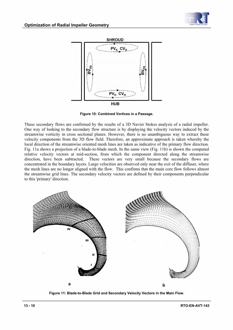
These secondary flows are confirmed by the results of a 3D Navier Stokes analysis of a radial impeller. One way of looking to the secondary flow structure is by displaying the velocity vectors induced by the streamwise vorticity in cross sectional planes. However, there is no unambiguous way to extract these velocity components from the 3D flow field. Therefore, an approximate approach is taken whereby the local direction of the streamwise oriented mesh lines are taken as indicative of the primary flow direction. Fig. 11a shows a projection of a blade-to-blade mesh. In the same view (Fig. 11b) is shown the computed relative velocity vectors at mid-section, from which the component directed along the streamwise direction, have been subtracted. These vectors are very small because the secondary flows are concentrated in the boundary layers. Large velocities are observed only near the exit of the diffuser, where the mesh lines are no longer aligned with the flow. This confirms that the main core flow follows almost the streamwise grid lines. The secondary velocity vectors are defined by their components perpendicular to this 'primary' direction.

a

b

Figure 11: Blade-to-Blade Grid and Secondary Velocity Vectors in the Main Flow.


RTO-EN-AVT-143 13 - 11

The four mesh lines in bold indicate the blade-to-blade surfaces where these secondary flow vectors are calculated. These surfaces correspond to mesh surfaces of the structured grid and are fully three-dimensional. Fig. 12 shows the intersection, in the meridional view, between these cross surfaces and the suction and pressure side of the blades.

Figure 12: Definition of Cross Sections in the Meridional Plane.

The secondary flow vectors in the four cross planes, defined here above, are plotted on Fig. 13 to 16.

The endwall passage vortices generated by the blade curvature are already present in cross plane I (Fig. 13). It is much stronger near the shroud because of the higher relative velocity and the thicker inlet boundary layer. In the curved part of the impeller inlet, one observes the start of the blade surface vortices, due to the meridional curvature. This vortex is already stronger on the suction side because of the higher velocity and thicker boundary layer. The blade surface vortex along the pressure side is very small because it is still close to the leading edge. It gets stronger near the shroud, where the relative velocity is higher.

In cross plane II (Fig. 14), the blade surface vortices are now developed on both sides but still stronger near the suction side. The passage vortex is larger at the shroud than at the hub. A lot of low energy fluid is accumulating in the shroud/suction side corner. This will be a dangerous area in terms of flow separation.


13 - 12 RTO-EN-AVT-143

Figure 13: Secondary Flow Velocity Vectors in Section I.

Figure 14: Secondary Flow Velocity Vectors in Section II.

The blade surface vortex along the suction side has nearly vanished between the cross planes II and III (Fig. 15),because, on this side, it is no longer fed by the meridional curvature. On the contrary, the one along the pressure side is still very strong, because it is located upstream in the meridional channel. The passage vortex is now mainly fed by the loading due to the Coriolis effect but weakened by the blade curvature effect. It is very weak near the hub because the local boundary layer is very thin as most of the boundary layer fluid is evacuated by the blade vortex on the pressure side. It is much stronger near the shroud because the boundary layer is thicker as it is continuously fed with low energy fluid by the pressure side blade vortex. In addition the loading is higher near the shroud.

Figure 15: Secondary Flow Velocity Vectors in Section III.


RTO-EN-AVT-143 13 - 13

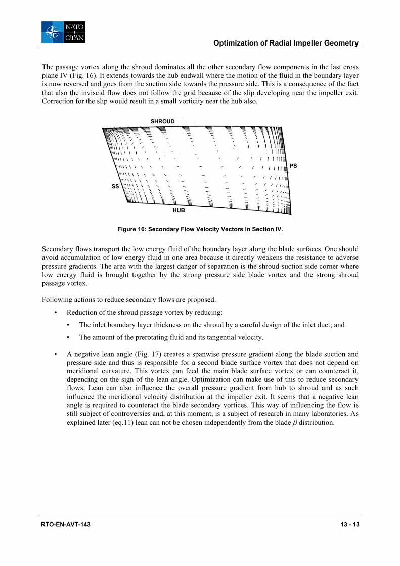
The passage vortex along the shroud dominates all the other secondary flow components in the last cross plane IV (Fig. 16). It extends towards the hub endwall where the motion of the fluid in the boundary layer is now reversed and goes from the suction side towards the pressure side. This is a consequence of the fact that also the inviscid flow does not follow the grid because of the slip developing near the impeller exit. Correction for the slip would result in a small vorticity near the hub also.

Figure 16: Secondary Flow Velocity Vectors in Section IV.

Secondary flows transport the low energy fluid of the boundary layer along the blade surfaces. One should avoid accumulation of low energy fluid in one area because it directly weakens the resistance to adverse pressure gradients. The area with the largest danger of separation is the shroud-suction side corner where low energy fluid is brought together by the strong pressure side blade vortex and the strong shroud passage vortex.

Following actions to reduce secondary flows are proposed.

• Reduction of the shroud passage vortex by reducing:

• The inlet boundary layer thickness on the shroud by a careful design of the inlet duct; and

• The amount of the prerotating fluid and its tangential velocity.

• A negative lean angle (Fig. 17) creates a spanwise pressure gradient along the blade suction and pressure side and thus is responsible for a second blade surface vortex that does not depend on meridional curvature. This vortex can feed the main blade surface vortex or can counteract it, depending on the sign of the lean angle. Optimization can make use of this to reduce secondary flows. Lean can also influence the overall pressure gradient from hub to shroud and as such influence the meridional velocity distribution at the impeller exit. It seems that a negative lean angle is required to counteract the blade secondary vortices. This way of influencing the flow is still subject of controversies and, at this moment, is a subject of research in many laboratories. As explained later (eq.11) lean can not be chosen independently from the blade β distribution.


13 - 14 RTO-EN-AVT-143

Figure 17: Effect of Negative Lean on the Pressure Distribution.

• A last way to influence the passage vortex is by means of the shroud tip clearance. The fluid in the shroud boundary layer of an unshrouded impeller, has a zero peripheral velocity in the absolute frame. In the relative frame, this results in a movement of the fluid from suction to pressure side, opposite to the shroud passage vortex (Fig. 18b). Moreover, the passage vorticity near the shroud is also opposite to the inviscid jet of fluid coming from the pressure side of the adjacent channel through the clearance. This jet therefore blows the low energy fluid away from the shroud suction side corner. The impact on the vortex structure is illustrated on Fig. 18a (shrouded) and 18b (unshrouded).

a b

Figure 18: Secondary Flow in a Shrouded (a) and Unshrouded (b) Impeller.

2.0 3D OPTIMIZATION

Taking into account the large importance of the secondary flow on performance and flow structure it is clear that any optimization requires the use of a full 3D flow analysis. Any inaccuracy of the flow predictor may lead to a false optimum and the use of a reliable but computational expensive 3D Navier-Stokes solver is therefore unavoidable. However the large amount of information provided and the complex interaction between the blade loading, meridional curvature, radius change and lean make a manual optimization very difficult and the support of advanced optimization techniques is very helpful.

Many optimization methods have been developed. However most of them require expensive performance evaluations on a large number of different geometries. The main drawbacks are the very large computer


RTO-EN-AVT-143 13 - 15

efforts that are required or the simplifications that are needed to obtain affordable and practical design times.

Following describes the design procedure developed at the VKI and its application to radial impeller optimization [5,6]. This 2 level optimization method aims for a fast, multipoint optimization in a multidisciplinary environment.

2.1 Optimization Method The optimization method is an extension to radial turbomachinery [5,6] of the approach described in [7]. The core of this knowledge-based design system (Fig. 19) is a GENETIC ALGORITHM in combination with an Artificial Neural Network (ANN) to PREDICT the performance of a candidate GEOMETRY proposed by the Genetic Algorithm. The ANN makes use of the knowledge acquired during previous designs of similar impellers and stored in a DATABASE. Once the fast optimization is finished, the optimized geometry is verified by means of an accurate Navier-Stokes solver (TRAF3D) and the results of this calculation are added to the DATABASE. This cycle is stopped when the Navier Stokes PERFORMANCE agrees with the ANN one so that no further improvements can be expected. In the other cases a new optimisation loop is started after a new LEARNING of the ANN on the new DATABASE. As the new DATABASE contains new information about impellers that are similar to the required one, one can expect that the next predictions by the ANN will be more accurate.

Figure 19: Flow Chart of a 2 Level Optimization Method.

The TRAF3DSP Navier-Stokes solver used in present study is an extension for radial compressors with splitter vanes of the TRAF3D solver [8]. All computations are performed on similar grids (230 000. points) to guarantee a comparable accuracy for all the samples stored in the database. This is important because any scatter in the information, due to grid dependence, could drive the optimisation process in a wrong direction.

The GA optimisation algorithm used in the present work is the genetic algorithm developed by David L. Carroll at University of Illinois [9]. Typically 100 generations are created each containing 50 samples using the Micro Genetic Algorithm. Binary coding is used with the elitist tournament selection strategy. The algorithm allows uniform cross-over with a probability of 0.5 and a jump mutation with a probability of 0.02.


13 - 16 RTO-EN-AVT-143

Following gives an overview of the different steps that have been taken to make the system faster by defining optimum parameter setting for Genetic Algorithm and Artificial Neural Network and introducing a technique to define a more representative DATABASE.

The quality of the Genetic Algorithm GA optimizer depends on:

• The required computational effort i.e. the number of performance evaluations that are needed to find that optimum (GA efficiency).

• The value of the optimum (GA effectiveness).

The GA software used in the VKI design system is the one developed by David L. Carroll [9]. The “optimum parameter settings” has been verified and adapted by means of a systematic study on two impellers defined respectively by 7 and 27 parameters [10]. Conclusions are based on the solution quality

minOFOFOFOF

qAV

GAAV

−−

=

measuring the degree to what the GA optimum GAOF ,approaches the real one minOF within a given effort (5000 function evaluations). AVOF is the average of the objective function over the complete design space. Hence a q value of 1 indicates that the global minimum value has been found.

The function evaluations for the numerical experiments are made by means of an ANN, trained on a database corresponding to the respective impeller geometries (7 or 27 parameters). A systematic analysis has been made to find the optimum values of substring length, selection scheme, population size, crossover and mutation probabilities has lead to a higher convergence rate and a lower Objective Function. An optimum setting results in a higher GA efficiency and improved effectiveness (Fig. 20).

Figure 20: GA Convergence for Standard and Optimized Parameter Setting for the 27 Parameter Test Radial Impeller Geometry Definitions.

Artificial Neural Networks (ANN)

The optimization cost depends on the number of cycles (GA optimizations and subsequent Navier Stokes analyses) that are required to find an accurate ANN predictor. An optimal use of the database information


RTO-EN-AVT-143 13 - 17

is therefore a must. The purpose of the ANN is not to reproduce the existing database with maximum accuracy but to predict the performance of new geometries it has not seen before i.e. to generalize. The standard back propagation is the most widely used learning algorithm for Artificial Neural Networks. The available samples are divided into training-, test- and validation sets.

The Training set contains the samples used for learning; that is to define the ANN parameters (i.e., weights).

The Test set contains the samples used only to assess the performance (generalization) of a fully-specified ANN (given weights and architecture).

The Validation set contains the samples used to tune the parameters (i.e., architecture, not the weights) of the ANN.

DATABASE

The main purpose of the DATABASE is to provide information about the relation between the geometry and performance. The more general and complete is this information, the more accurate may be the ANN and the closer the first optimum geometry, defined by the GA, will be to the real optimum. A systematic research [11] has shown that using a Design Of Experiment technique (DOE) allows a drastic reduction of the number of samples in the database without considerable loss of information. Randomly generated databases are all different and show an error that can be three times larger than the one of a DOE defined database.

2.2 Radial Impeller Geometry Definitions The convergence speed is strongly influenced by the number of unknown that are needed to define the optimum geometry. Selecting parameters that have a direct relation to the performance, such as blade angles and pitch to chord ratio, allow a more straightforward relation between geometry and performance. The corresponding ANN is simpler and more easily defined. Hence less iterations will be needed to reach agreement between the ANN- and the Navier Stokes predictions. It is also important to select a geometry definition that is sufficiently general to allow the reconstruction of a wide variety of geometries in order not to exclude the optimum one.

The use of Bézier polynomials allows a 3D definition of turbomachines with a number of parameters that can be as low as 7 for 2D geometries and 27 for 3D radial impellers. A three-dimensional radial impeller geometry is defined by the meridional contour at hub and shroud (21a) and the camber line of the blade sections (Fig. 21b) at both locations. Hub and shroud meridional contours are defined by third order Bézier curves (Fig. 21a). The unknown that need to be defined during the optimisation process are the values of (X1,R1) and (X2,R2) at hub and shroud. The leading edge and trailing edge section points, (X0,R0) and (X3,R3), are predefined. They are the result of a preliminary 1D design where one accounts also for the off-design operation. The points A and B are dependent variables and adjusted to assure a smooth inlet and outlet contour.


13 - 18 RTO-EN-AVT-143

a

b

Figure 21: Parameterization of the Meridional Contour and the Blade Angle β.

The coordinates θ of the blade camber line are computed from the prescribed distribution of the angle β, between the meridional plane m and the camberline S (Fig. 22a).

R dθ = dm tanβ (11)

The β distributions at hub and tip are defined by cubic Bézier curves.

β(u)= β3 (u-1)3 + β2 (u-1)2 u+ β1 (u-1)u2 + β0 u3 (12)

where u is the non-dimensionalized meridional length. Four parameters (β0 to β3) need to be defined at hub and shroud. Together with the parameters of the meridional contour, this makes only 16 parameters for the complete 3D definition of a radial impeller geometry. It may increase to 26 parameters when also splitter vanes are introduced.


RTO-EN-AVT-143 13 - 19

a

b

Figure 22: Blade camberline definition (a) and restriction of the design space (b).

The circumferential extend of the blades TELE θθ − at hub and shroud are related by the maximum lean that is allowed at leading- and trailing edge and constitute a limitation on the β distribution.

As it is of no interest to analyse impeller geometries that can not be manufactured or assembled, the optimisation process can be accelerated by limiting the design parameters to realistic values. Limiting the extend of parameter variations to feasible geometries (Fig. 22b), reduces the design space and favours a faster convergence.

2.3 Objective Function The objective function based on Navier Stokes results measures in how far the geometry satisfies the flow-requirements and reaches the performance goals that have been set forward. The same objective function, but based on ANN predictions, drives the GA towards the optimum geometry.

High efficiency however is not the only design objective of an aerodynamic shape optimization. A good design must also:

• Provide good off-design performance over a prescribed operating range (multipoint optimization); and

• Respect the mechanical and manufacturing constraints (multidisciplinary optimization).

Hence the problem is the minimization of a non linear objective function in several variables, subject to several constraints (mechanical, manufacturing and flow constraints). A possible approach to this problem is the definition of a pseudo-objective function (OF) by adding penalty terms that are increasing when the constraints [7] are violated. Following lists some contributions to the global objective function that one has been using in different applications:

SidesideGeomGeommecamecaVelocVelocBCBC PwPwPwPwPwPwOF +++++= ηη (13)

The weight factors “w” allow changing the importance of the different contributions (i.e. performance versus mechanical constraints).


13 - 20 RTO-EN-AVT-143

PBC This penalty enforces the user-imposed boundary conditions or requirements at the inlet and outlet of the computational domain, such as the inlet flow angle (β1), the outlet flow angle (β2), the pressure ratio ( oPP 12 / ), the mass flow etc.

The penalties for not respecting boundary conditions start increasing when the actual value differs from the target value by more than a predefined tolerance. Following is a typical expression for mass flow penalty:

( )[ ] 2.0,02./max −−= reqreqactmass mmmP (14)

i.e. the penalty starts increasing when the difference between the actual and the required mass flow exceeds 2%. The rate of increase is defined by wi (Fig. 23).

Figure 23: Weak Formulation of Constraint.

This weak formulation of the constraints does not guarantee that the constraints will be satisfied in a strict way. Any violation of the constraint will result in an increase of the “OF” that may however be compensated by a decrease of another penalty term. However this formulation shows a more easy convergence to the constraint optimum, even when starting outside the feasible domain.

Pη penalizes geometries with low efficiency (η) or high loss coefficient (ω).

PVeloc is the penalty for non-optimum velocity distribution. Navier Stokes solvers are not always reliable in terms of transition modelling and large discontinuous variations of penalty function could occur when the position of the transition point is changing. Analyzing the velocity distribution may help to make a selection between blades that have nearly the same loss coefficient or to favour the ones that are better in terms of NPSH.

The aim of optimization methods is to design blades that perform also well at off-design operating conditions. One must therefore avoid designing blade geometries that have very good performance in a narrow range around the design point but are likely to separate (with high losses) at slightly off design conditions. The simplest approach is to account for the changes on the velocity distribution that can be expected at off-design. This increases the chances for good performance of the blade over a wide range of operating conditions without the cost of several Navier-Stokes computations at off-design conditions. Experience has shown that imposing limitations on the velocity distribution in terms of deceleration, negative loading and loading difference between main blade and eventual splitter blade has a favourable effect on the operating range.

Following are some of the velocity penalties that have been formulated. They are based on the isentropic velocity on the blade suction and pressure side. The velocities are calculated based on the static pressure and constant rotary stagnation pressure (assuming isentropic flow) (eq.6). The purpose is to penalize velocity distributions that are known of not being optimal such as distributions having a high velocity peak


RTO-EN-AVT-143 13 - 21

followed by a strong deceleration near the leading edge (Fig. 24). Penalty for negative loading is proportional with the integral between suction and pressure side velocity distribution when the pressure side velocity is higher than the suction side one. Other terms penalize the difference in loading between the main blade and eventual splitter vanes taking into account the difference in blade length. Any eventual difference in mass flow between the two channels at both sides of the splitter vane will further increase the penalty.

Figure 24: Penalties on Velocity Distribution.

Penalizing the spanwise variation of the flow at the exit may also have a favourable effect on the downstream diffuser and hence on stage efficiency and range.

PMeca is the penalty for violating the mechanical constraints. An important parameter in radial impellers is the blade lean angle in the axial part or rake angle in the radial part. The centrifugal forces create large stresses in the blade root section of non radial blades. Maximum lean angles must therefore be imposed. The limiting value is based on experience, correlations or FEA analysis and depends on expected life time.

The penalties for violation of the mechanical constraints are a one sided formulation of the definition used for boundary conditions (eq. 14). The penalty starts increasing when the constraint is violated. As already mentioned, this way of imposing a constraint does not guarantee that the constraints will be rigorously respected but it has the advantage that the geometries violating the constraints, are still available to drive the geometry back to the feasible domain. A strong formulation of the mechanical constraints is discussed in section 2.4.

PGeom is the penalty for violation of the geometrical constraints.

Geometrical constraints do not influence the mechanical integrity but aim to respect restrictions such as maximum length and assure dimensional agreement with upstream or downstream components. They may also result from manufacturing (casting) considerations.

A possible argument to introduce geometrical constraints is to favour geometrical features that are known to improve the design or off-design performance i.e. limited change of curvature, some prescribed lean or sweep laws, limiting camber of the uncovered turbine suction side, etc.


13 - 22 RTO-EN-AVT-143

PSide is the penalty for violating the side constraints and depends on the application. Manufacturing- and maintenance cost may also be an important issue and some geometries can be favoured by formulating an appropriate penalty.

2.4 Mutidisciplinary Optimization Maximized performance is of no use if the mechanical integrity of a design is not guaranteed. Geometries that are violating these constraints must be eliminated from the optimization process. Most of them result from a combination of different design parameters and cannot be avoided by reducing the feasible range of the individual design parameters.

A possible way of calculating the multidisciplinary OF is shown on Fig. 25. It is a extension of the flow chart shown in Fig. 19. The GA, searching for the optimum geometry, gets its input as well from the Finite Element stress Analysis (FEA) as from the Navier Stokes flow solver.

Figure 25: Multidisciplinary Optimization Flow Chart.

The main advantages of such an approach are:

• Only one “master” geometry is used i.e. the one defined by the geometrical parameters used in the GA optimizer is input for all analyses.

• A more direct convergence to the optimum geometry without iterations between the optimized aerodynamic geometry and the mechanical acceptable one.

• The possibility to do parallel calculations. Both FEA and NS analysis can be made in parallel if each discipline is independent i.e. if stress calculations do not need the pressure distribution on the blades or flow calculations can neglect the geometry deformations.

• The GA is driven by a more accurate version of the pseudo OF whereby in analogy with the flow analysis one can reduce the computational effort by formulating an approximate prediction model for mechanical characteristics.

An example of such a correlation is shown on Fig. 26a. It results from a systematic FEA study of the stresses in a 2D unshrouded radial impeller Fig. 26b. It defines the limits of acceptable combinations of blade angle and blade height in function of maximum stress. One observes an increase of stresses in the hub region with increasing leading edge angle β because the centrifugal forces become more perpendicular to the blade. Larger blade heights increase the stresses because of increased overhang.


RTO-EN-AVT-143 13 - 23

Impellers with larger blade height are likely to perform better because of smaller clearance and friction losses. However they require larger leading edge angles to achieve the optimum incidence. Lines of constant stresses define the limits of the design space for the optimization.

a b

Figure 26: Variation of Maximum von Mises Stress as a Function of Blade Height and Leading Edge Angle ßLE.

2.5 Multipoint Optimization Multipoint optimization aims for a design that performs well in more than one operating point. The simplest straightforward approach is to analyze each candidate geometry in the different operating points and to calculate a weighted sum of the corresponding Objective Functions.

332211 ... OFwOFwOFwOF ++= (15)

where wi is the weight given to the objective functions iOF corresponding to each operating point.

This approach is not only very expensive in terms of computer effort (one Navier Stokes solver for each operating point), it may also lead to convergence problems. Changing the operating point in pumps, means imposing a different pressure ratio or mass flow. As the stability limit is not a priori known there is no guarantee that the Navier Stokes solver will converge at the modified pressure ratio. Fewer problems occur when the off-design corresponds to a change of inlet conditions (change of rotor inlet conditions because of different IGV setting angle or change of diffuser inlet flow by changing rotor operating point).

Fig. 27 shows the convergence history of an application where the off-design operation corresponds to different settings of the Inlet Guide Vane (IGV). One observes a decrease of the efficiency penalty based on NS at all 3 operating points and a gradual improvement of the ANN predictions. The absolute values are quite different for each operating point because of the decreasing weight for operating point 2 and 3. One observes that after 33 iterations the ANN predictions agree well with the Navier Stokes predictions which allows concluding that the geometry optimized with the ANN is also optimum according to the Navier Stokes calculations.


13 - 24 RTO-EN-AVT-143

OP1

OP2

OP3

Figure 27: Multipoint Optimization Convergence at the Operating Points OP1, OP2 and OP3.

2.6 Application to Radial Impeller Design Following example concerns the optimization of a radial impeller. The meridional contour is shown on Fig. 28. The arrows indicate the Bézier parameters that are allowed to change. The squares indicate the dependent variables. The latter ones are automatically adjusted to assure a continuous hub and shroud contour at inlet and outlet. The optimization starts from a database containing 35 geometries and the corresponding results of a Navier Stokes calculation. The penalty function accounts for efficiency penalty (max. efficiency not reached), negative loading on main blade and splitter blades, mass flow error and unequal mass flow on both sides of the main blade. The largest weight is put on high efficiency.

Figure 28: Meridional Contour of Radial Impeller.

The convergence history is illustrated by the efficiency penalty shown on Fig. 29. Negative iteration numbers correspond to the samples in the database. One observes a big scatter with some rather high penalties. This is the consequence of a systematic scanning of the design space by means of DOE. It makes the learning process more efficient because it allows the ANN to learn what distinguishes a good from a bad impeller. The impellers defined by the optimizer show on average a much lower penalty (higher efficiency) than the database samples. In the first part one observes a big scatter with large discrepancies between the penalty based on the Navier Stokes results and the one based on the ANN. These discrepancies are due to the incorrect ANN predictions and disappear when the ANN becomes more


RTO-EN-AVT-143 13 - 25

accurate because trained on a larger database. Good optimum geometries are found by the optimizer only after the ANN performance evaluator became more accurate i.e. about 50 iterations when the discrepancies between the ANN and Navier Stokes predictions disappear. Continuing the optimization procedure, after the ANN and NS predictions agree, does not bring any further improvement as shown on Fig. 29.

Figure 29: Convergence History (Efficiency Penalty).

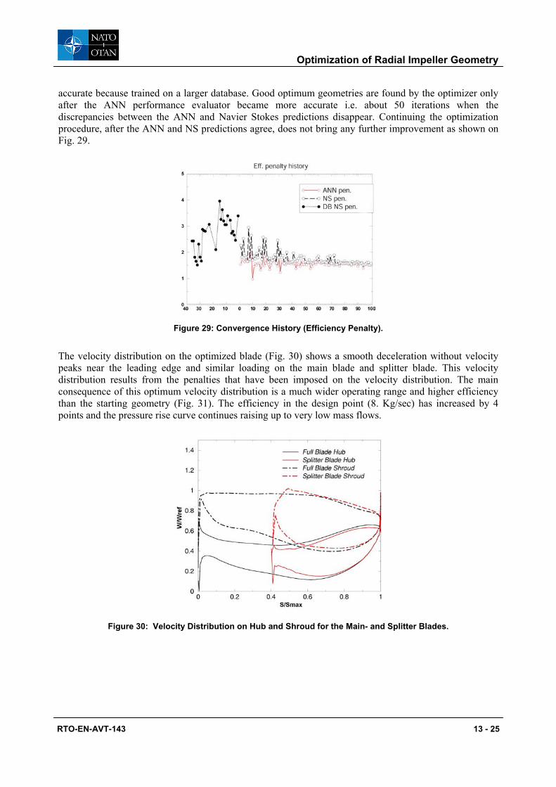
The velocity distribution on the optimized blade (Fig. 30) shows a smooth deceleration without velocity peaks near the leading edge and similar loading on the main blade and splitter blade. This velocity distribution results from the penalties that have been imposed on the velocity distribution. The main consequence of this optimum velocity distribution is a much wider operating range and higher efficiency than the starting geometry (Fig. 31). The efficiency in the design point (8. Kg/sec) has increased by 4 points and the pressure rise curve continues raising up to very low mass flows.

Figure 30: Velocity Distribution on Hub and Shroud for the Main- and Splitter Blades.


13 - 26 RTO-EN-AVT-143

a

b

Figure 31: Pressure Rise (a) and Efficiency (b) versus Mass Flow.

2.7 Conclusions It has been shown how a two level optimization can considerably decrease the computational effort that is needed to design turbomachinery components.

Further improvements of the convergence has been obtained by an optimum parameter settings for the Genetic Algorithm, the use of DOE for the definition of the database and by an optimized learning technique for the ANN.

The penalties on velocity distribution do not only result in improved performance at design point but also contribute to a much wider operating range.

REFERENCES [1] Baljé O., “Turbomachines - a guide to design, selection and theory”, J. Wiley & Sons, New York,

1981.

[2] Smith A.G., "On the generation of the Streamwise Component of Vorticity for Flows in a Rotating Passage", Aeronautical Quartely, Vol. 8, 1957, pp. 369-383.

[3] Hawthorn W.R., "Secondary Vorticity in Stratified Compressible Fluids in Rotating Systems", Cambridge Univ. Eng. Dept., CUED/A-Turbo/TR 63.

[4] Hirsch Ch., Kang. S. & Pointel G., "A Numerically Supported Investigation of the 3D Flow in Centrifugal Impellers - Part II : Secondary Flow Structure", ASME paper 96-GT-152, 1996.

[5] Cosentino R., Alsalihi Z., Van den Braembussche R.A.; “Expert system for Radial Impeller Optimization”, Paper presented at the 4th European conference on Turbomachinery, Firenze, March 20-23, 2001.

[6] Rini P., Alsalihi A, Van den Braembussche R.A.; “Evaluation of a Design Method for Radial Impellers Based on Artificial Neural Network and Genetic Algorithm”, Paper presented at the 5th ISAIF Conference, Gdansk, Sept. 4-7, 2001.

[7] Pierret, S., Van den Braembussche R.A..; “Turbomachinery Blade Design using a Navier-Stokes solver and Artificial Neural Network”. ASME Trans., Journal of Turbomachinery, Vol 121, No 2, 1999 (pp. 326-332).


RTO-EN-AVT-143 13 - 27

[8] Arnone, A. (1994). “Viscous Analysis of Three Dimensional Rotor Flow Using a Multigrid Method”. ASME Journal of Turbomachinery, Vol. 116, pages 435-445.

[9] Carroll, D.L. (2001). FORTRAN Genetic Algorithm (GA) Driver version 1.7.1a. Available at URL: http://cuaerospace.com/carroll/ga.html.

[10] Harinck, J. Alsalihi Z., Van Buijtenen J.P., Van den Braembussche R.A.; “Optimization of a 3D Radial Turbine by means of an improved Genetic Algorithm”, Proceedings of the 5th European Conference on Turbomachinery, page 1033-1042, March, 2005.

[11] Kostrewa K. ; “Optimization of Radial Turbines by means of Design Of Experiment”, VKI-PR-2003-17.

http://cuaerospace.com/carroll/ga.html


13 - 28 RTO-EN-AVT-143

Optimization of Radial Impeller Geometry - CiteSeerX

Documents

Transcript of Optimization of Radial Impeller Geometry - CiteSeerX