Geophys. J. Int. (2011) 187, 754–772 doi: 10.1111/j.1365-246X.2011.05172.x

GJI

Gra

vity

,ge

ode

syan

dtide

s

Source geometry estimation using the mass excess criterion toconstrain 3-D radial inversion of gravity data

Vanderlei C. Oliveira, Jr,1 Valeria C. F. Barbosa1 and Joao B. C. Silva2

1Observatorio Nacional, Gal. Jose Cristino, 77, Sao Cristovao, Rio de Janeiro, 20921-400, Brazil. E-mail: vandscoelho@gmail.com2 Universidade Federal do Para, Dep. Geofısica CG, Caixa Postal 1611, 66017-900, Belem, Para, Brazil

Accepted 2011 July 26. Received 2011 July 26; in original form 2010 October 13

S U M M A R YWe present a gravity-inversion method for estimating the geometry of an isolated 3-D source,assuming prior knowledge about its top and density contrast. The subsurface region containingthe geological sources is discretized into an ensemble of 3-D vertical prisms juxtaposed in thevertical direction of a right-handed coordinate system. The prisms’ thicknesses and densitycontrasts are known, but their horizontal cross-sections are described by unknown polygons.The horizontal coordinates of the polygon vertices approximately represent the edges ofhorizontal depth slices of the 3-D geological source. The polygon vertices of each prism aredescribed by polar coordinates with an unknown origin within the prism. Our method estimatesthe horizontal Cartesian coordinates of the unknown origin and the radii associated with thevertices of each polygon for a fixed number of equally spaced central angles from 0o to 360o.By estimating these parameters from gravity data, we retrieve a set of vertically stacked prismswith polygonal horizontal sections that represents a set of juxtaposed horizontal depth slices ofthe estimated source. This set, therefore, approximates the 3-D source’s geometry. To obtainstable estimates we impose constraints on the source shape. The judicious use of first-orderTikhonov regularization on either all or a few parameters allows estimating both vertical andinclined sources whose shapes can be isometric or anisometric. The estimated solution, despitebeing stable and fitting the data, will depend on the maximum depth assumed for the set ofjuxtaposed 3-D prisms. To reduce the class of possible solutions compatible with the gravityanomaly and the constraints, we use a criterion based on the relationship between the data-misfit measure and the estimated total-anomalous mass computed along successive inversions,using different tentative maximum depths for the set of assumed juxtaposed 3-D prisms. Inapplying this criterion, we plotted the curve of the estimated total-anomalous mass mt versusdata-misfit measure s for the range of different tentative maximum depths. The tentative valuefor the maximum depth producing the smallest value of data-misfit measure in the mt ×s curveis the best estimate of the true (or minimum) depth to the bottom of the source, depending onwhether the true source produces a gravity anomaly that is able (or not) to resolve the depth tothe source bottom. This criterion was theoretically deduced from Gauss’ theorem. Tests withsynthetic data shows that the correct depth-to-bottom estimate of the source is obtained if theminimum of s on the mt × s curve is well defined; otherwise this criterion provides just alower bound estimate of the source’s depth to the bottom. These synthetic results show thatthe method efficiently recovers source geometries dipping at different angles. Test on real datafrom the Matsitama intrusive complex (Botswana) retrieved a dipping intrusion with variabledips and strikes and with bottom depth of 8.0 ± 0.5 km.

Key words: Numerical solutions; Inverse theory; Gravity anomalies and Earth structure.

1 I N T RO D U C T I O N

The reconstruction of 3-D (or 2-D) geological sources from a dis-crete set of gravity data measured at the Earth’s surface usually fol-lows two strategies. The first one is the interactive gravity forward

modelling and the second strategy comprises the gravity-inversionmethods.

The interactive gravity forward modelling consists in inferring arepresentation of the 3-D (or 2-D) geometry of geological sourcesin the subsurface that fits the observed gravity data. Hence, the

754 C© 2011 Obsevatorio Nacional

Geophysical Journal International C© 2011 RAS

Geophysical Journal International at O

bservatório N

acional on January 9, 2014http://gji.oxfordjournals.org/

Dow

nloaded from

3-D radial inversion of gravity data 755

interactive gravity forward modelling requires the specification oftentative source geometry and it allows the interactivity and flex-ibility of introducing geological information about the study areaat the interpreter’s discretion. Therefore, the interpreter’s concep-tion about the geology of the study area is incorporated in a directway. However, this task involves an exhaustive, tedious and time-consuming trial-and-error procedure wherein the interpreter mustsupervise both the data fit and the construction of geologicallymeaningful sources. Most recently substantial effort has been de-voted towards making the 3-D (or 2-D) interactive gravity forwardmodelling more attractive and operational. For example, Silva &Barbosa (2006) and Silva Dias et al. (2009), respectively, assum-ing 2-D and 3-D sources, combined the best features of interactiveforward modelling (the interactivity and flexibility of introducinggeological information) and of automatic inversion (the facility ofautomatically fitting the observations). These authors’ approachesare similar to a standard interactive gravity forward modelling butdiffer from it in automatically fitting the observations and in requir-ing from the interpreter only the knowledge of the skeletal outlinesof the sources expressed by simple geometric elements such aspoints and lines. Through these approaches the interpreter specifiesa set of skeletal outlines (points and lines) of the presumed sourcesand the method finds a solution that concentrates the anomalousmass about these skeletons. Therefore, the interpreter is not re-quired to specify the complete source geometry. Calcagno et al.(2008) combined the measurements of the structural data on out-crops or in boreholes (e.g. dip measurements, stratifications or folia-tions related to the contacts) and a set of rules derived from the rockrelationships between formations (e.g. the chronology of geologicalevents or different rock relations between formations) with potentialfield data (gravity and magnetic data). In Calcagno et al.’s (2008)approach the judicious combination of geological maps, boreholedata, structural data, physical properties of the rocks, gravity and/ormagnetic data allows building 3-D geological models.

The reconstruction of 3-D (or 2-D) geological sources throughthe gravity-inversion methods has been proposed by many authors.Most inversion methods estimate a 3-D density-contrast distribu-tion by assuming a piecewise constant function defined on a user-specified grid of cells. However, the problem of estimating a 3-D(or 2-D) density-contrast distribution from gravity data only is anill-posed problem because its solution is neither unique nor stable.To transform this ill-posed problem into a well-posed one, thesegravity-inversion methods usually use the Tikhonov regularizationmethod (Tikhonov & Arsenin 1977). It consists in formulating aconstrained inverse problem by minimizing an unconstrained func-tion composed by (1) the data-misfit function, consisting of a normof the difference between the observed and predicted data, and (2)the regularizing function defined in the parameter (model) spacewhose minimization imposes physical or geological attributes on asolution. Two regularizing functions commonly used in geophysicsare the zeroth- and first-order Tikhonov regularizations. Both reg-ularizing functions impose a smooth character on the estimateddensity-contrast distribution and they concentrate the excess (ordeficiency) of mass at the borders of the interpretation region, irre-spective of the true source depth. Some examples of this tendencyare given in Portniaguine & Zhdanov (1999), their figs 1(c), 2(c)and 3(c), Barbosa et al. (2002), their fig. 5 and Silva et al. (2001a),their figs 7 and 8. Over the last years, efforts have been directed tocounteract the tendency of producing a blurred density-contrast dis-tribution concentrated at the borders of the interpretation region. Inthis context, some non-smoothing regularization functions arose inestimating the density-contrast distribution in the subsurface. Most

of these non-smoothing regularizers retrieve sharper images of ge-ological sources as compared with the smoothing regularizers, butthey require larger amount of prior information. Some examplesare given by the following authors: Last & Kubik’s (1983) methodproduced compact and homogeneous solutions; Barbosa & Silva(1994) generalized the moment-of-inertia functional proposed byGuillen & Menichetti (1984) and Barbosa et al. (1999a) applied itto reconstruct a heterogeneous sedimentary pack; Bertete-Aguirreet al. (2002) used TV regularization, whose stabilizing functional isthe �1-norm of the first-order derivative of the parameters along thehorizontal and vertical directions; Portniaguine & Zhdanov (1999)minimized a measure of the total volume within the estimated sourcein which the physical property gradient is non-null in 3-D gravityinversion; Silva & Barbosa (2006) and Barbosa & Silva (2006) ex-tended Barbosa & Silva’s (1994) method for multiple sources withmultiple axes and points; Silva Dias et al. (2009) proposed an adap-tive learning scheme extending Silva & Barbosa’s (2006) methodto 3-D gravity inversion.

Although the inversion methods that parametrize the Earth’s sub-surface into a grid of cells (2-D or 3-D) to estimate a density-contrastdistribution allow an enormous flexibility because they can estimatearbitrary variations, the usual Tikhonov regularizations of orderszero and one lead to blurred source images whose maximum andminimum estimated values occur at the boundary of the discretizedregion. To retrieve a sharper image of geological sources, this in-version approach requires a substantial amount of prior informationabout the source. A second gravity-inversion approach has beenadopted by a few authors to obtain estimates of 3-D (or 2-D) geo-logical source through an interpretation model that eliminates mostof the above-mentioned difficulties. In this case the interpretationmodel consists either of a horizontally infinite prism with polygonalcross-section or of a polyhedral body that delineates the contour of,respectively, 2-D or 3-D isolated sources. Hence, the physical prop-erty (density contrast) of the body is assumed to be known and theparameters to be estimated are the geometric elements that definethe boundary of a polygonal cross-section or a polyhedral body.Moraes & Hansen (2001), for example, approximated the 3-D geo-logical body by a homogeneous polyhedral body and estimated itsvertices using the gravity data and the first-order Tikhonov regu-larization. Silva & Barbosa (2004) inverted the gravity data for thegeometry of an isolated causative body by representing it as a 2-Dhorizontal prism with a polygonal cross-section defined by verticeswhich are described in polar coordinates referred to an origin insidethe source. The parameters to be estimated in this case are the radiiassociated with the polygon vertices for a fixed number of equallyspaced central angles from 0o to 360o. They used a wide variety ofconstraints to stabilize the solutions and to introduce informationabout the source shape. Some examples of possible a priori infor-mation are the isometry, the convexity and the concentration of themass along preferred directions. Wildman & Gazonas (2009) de-veloped gravity- and magnetic-inversion methods for retrieving thegeometries of 2-D or 3-D multiple sources by assuming the knowl-edge of their physical properties and representing these geometriesby a tree-data structure. These authors approximated the geologicalsources by an interpretation model consisting either of 2-D prismswith polygonal sections or of polyhedral bodies and estimated thesources geometry in two steps. In the first step, the initial geometryconsists of a simple rectangle that is iteratively modified by scal-ing and translation transformations to determine the approximatesize and location of the source. Next, an optimizing stage gives amore accurate image of the source by dividing the leaf nodes ofthe tree into the union of two separate convex polygons along one

C© 2011 Obsevatorio Nacional, GJI, 187, 754–772

Geophysical Journal International C© 2011 RAS

at ObservatÃ

³rio Nacional on January 9, 2014

http://gji.oxfordjournals.org/D

ownloaded from

756 V. C. Oliveira, Jr, V. C. F. Barbosa and J. B. C. Silva

or more angles. Luo (2010) proposed a gravity-inversion methodto estimate the geometry of isolated 2-D source adopting Bayesianmodel inference approach which is implemented via the reversiblejump Markov chain Monte Carlo algorithm. This method estimates,in the x−z space beneath the Earth’s surface, the number of ver-tices (and their x- and z-coordinates) that describe a 2-D polygonalcross-section and approximately delineate the edges of an isolated2-D geological source.

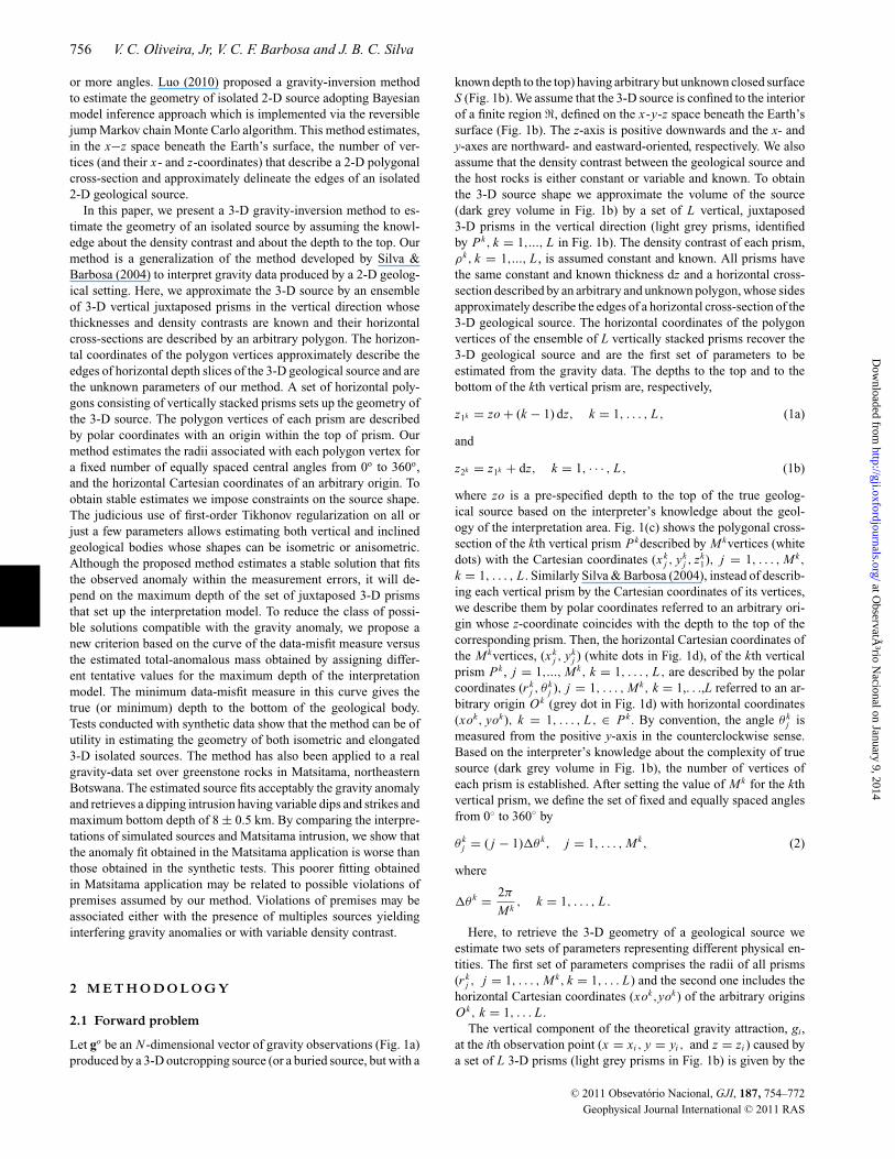
In this paper, we present a 3-D gravity-inversion method to es-timate the geometry of an isolated source by assuming the knowl-edge about the density contrast and about the depth to the top. Ourmethod is a generalization of the method developed by Silva &Barbosa (2004) to interpret gravity data produced by a 2-D geolog-ical setting. Here, we approximate the 3-D source by an ensembleof 3-D vertical juxtaposed prisms in the vertical direction whosethicknesses and density contrasts are known and their horizontalcross-sections are described by an arbitrary polygon. The horizon-tal coordinates of the polygon vertices approximately describe theedges of horizontal depth slices of the 3-D geological source and arethe unknown parameters of our method. A set of horizontal poly-gons consisting of vertically stacked prisms sets up the geometry ofthe 3-D source. The polygon vertices of each prism are describedby polar coordinates with an origin within the top of prism. Ourmethod estimates the radii associated with each polygon vertex fora fixed number of equally spaced central angles from 0o to 360o,and the horizontal Cartesian coordinates of an arbitrary origin. Toobtain stable estimates we impose constraints on the source shape.The judicious use of first-order Tikhonov regularization on all orjust a few parameters allows estimating both vertical and inclinedgeological bodies whose shapes can be isometric or anisometric.Although the proposed method estimates a stable solution that fitsthe observed anomaly within the measurement errors, it will de-pend on the maximum depth of the set of juxtaposed 3-D prismsthat set up the interpretation model. To reduce the class of possi-ble solutions compatible with the gravity anomaly, we propose anew criterion based on the curve of the data-misfit measure versusthe estimated total-anomalous mass obtained by assigning differ-ent tentative values for the maximum depth of the interpretationmodel. The minimum data-misfit measure in this curve gives thetrue (or minimum) depth to the bottom of the geological body.Tests conducted with synthetic data show that the method can be ofutility in estimating the geometry of both isometric and elongated3-D isolated sources. The method has also been applied to a realgravity-data set over greenstone rocks in Matsitama, northeasternBotswana. The estimated source fits acceptably the gravity anomalyand retrieves a dipping intrusion having variable dips and strikes andmaximum bottom depth of 8 ± 0.5 km. By comparing the interpre-tations of simulated sources and Matsitama intrusion, we show thatthe anomaly fit obtained in the Matsitama application is worse thanthose obtained in the synthetic tests. This poorer fitting obtainedin Matsitama application may be related to possible violations ofpremises assumed by our method. Violations of premises may beassociated either with the presence of multiples sources yieldinginterfering gravity anomalies or with variable density contrast.

2 M E T H O D O L O G Y

2.1 Forward problem

Let go be an N -dimensional vector of gravity observations (Fig. 1a)produced by a 3-D outcropping source (or a buried source, but with a

known depth to the top) having arbitrary but unknown closed surfaceS (Fig. 1b). We assume that the 3-D source is confined to the interiorof a finite region �, defined on the x-y-z space beneath the Earth’ssurface (Fig. 1b). The z-axis is positive downwards and the x- andy-axes are northward- and eastward-oriented, respectively. We alsoassume that the density contrast between the geological source andthe host rocks is either constant or variable and known. To obtainthe 3-D source shape we approximate the volume of the source(dark grey volume in Fig. 1b) by a set of L vertical, juxtaposed3-D prisms in the vertical direction (light grey prisms, identifiedby Pk, k = 1,..., L in Fig. 1b). The density contrast of each prism,ρk, k = 1,..., L , is assumed constant and known. All prisms havethe same constant and known thickness dz and a horizontal cross-section described by an arbitrary and unknown polygon, whose sidesapproximately describe the edges of a horizontal cross-section of the3-D geological source. The horizontal coordinates of the polygonvertices of the ensemble of L vertically stacked prisms recover the3-D geological source and are the first set of parameters to beestimated from the gravity data. The depths to the top and to thebottom of the kth vertical prism are, respectively,

z1k = zo + (k − 1) dz, k = 1, . . . , L , (1a)

and

z2k = z1k + dz, k = 1, · · · , L , (1b)

where zo is a pre-specified depth to the top of the true geolog-ical source based on the interpreter’s knowledge about the geol-ogy of the interpretation area. Fig. 1(c) shows the polygonal cross-section of the kth vertical prism Pkdescribed by Mkvertices (whitedots) with the Cartesian coordinates (xk

j , ykj , zk

1), j = 1, . . . , Mk,

k = 1, . . . , L . Similarly Silva & Barbosa (2004), instead of describ-ing each vertical prism by the Cartesian coordinates of its vertices,we describe them by polar coordinates referred to an arbitrary ori-gin whose z-coordinate coincides with the depth to the top of thecorresponding prism. Then, the horizontal Cartesian coordinates ofthe Mkvertices, (xk

j , ykj ) (white dots in Fig. 1d), of the kth vertical

prism Pk , j = 1,..., Mk, k = 1, . . . , L , are described by the polarcoordinates (r k

j , θkj ), j = 1, . . . , Mk, k = 1,. . .,L referred to an ar-

bitrary origin Ok (grey dot in Fig. 1d) with horizontal coordinates(xok, yok), k = 1, . . . , L , ∈ Pk . By convention, the angle θ k

j ismeasured from the positive y-axis in the counterclockwise sense.Based on the interpreter’s knowledge about the complexity of truesource (dark grey volume in Fig. 1b), the number of vertices ofeach prism is established. After setting the value of Mk for the kthvertical prism, we define the set of fixed and equally spaced anglesfrom 0◦ to 360◦ by

θ kj = ( j − 1)�θ k, j = 1, . . . , Mk, (2)

where

�θ k = 2π

Mk, k = 1, . . . , L .

Here, to retrieve the 3-D geometry of a geological source weestimate two sets of parameters representing different physical en-tities. The first set of parameters comprises the radii of all prisms(rk

j , j = 1, . . . , Mk, k = 1, . . . L) and the second one includes thehorizontal Cartesian coordinates (xok,yok) of the arbitrary originsOk, k = 1, . . . L .

The vertical component of the theoretical gravity attraction, gi,at the ith observation point (x = xi , y = yi , and z = zi ) caused bya set of L 3-D prisms (light grey prisms in Fig. 1b) is given by the

C© 2011 Obsevatorio Nacional, GJI, 187, 754–772

Geophysical Journal International C© 2011 RAS

at ObservatÃ

³rio Nacional on January 9, 2014

http://gji.oxfordjournals.org/D

ownloaded from

3-D radial inversion of gravity data 757

Figure 1. Schematic representation of (a) gravity anomaly (contour lines) produced by (b) a 3-D anomalous source (dark grey volume limited by the closedsurface S). The interpretation model in (b) consists of a set of L vertical, juxtaposed 3-D prisms Pk , k = 1,..., L ,(light grey prisms) in the vertical direction ofa right-handed coordinate system. (c) Polygonal cross-section of the kth vertical prism Pk described by Mk vertices (white dots) with the Cartesian coordinates(xk

j , ykj , zk

1), j = 1, . . . , Mk , k = 1, . . . , L . (d) Representation of the Mkvertices of the kth vertical prism Pk , (xkj , yk

j ), j = 1,..., Mk , k = 1, . . . , L , by polar

coordinates (rkj , θ

kj ), j = 1, . . . , Mk , k = 1, . . . , L , (white dots), referred to an arbitrary origin Ok (grey dot) with horizontal Cartesian coordinates (xok , yok ),

k = 1, . . . , L , (black dot).

non-linear relationship

gi ≡ gi (xi , yi , zi ) =L∑

k=1

f ki (rk, xok, yok, �k

, ρk), i = 1,..., N , (3)

where N is the number of gravity measurements, rk ≡ (rk1 , ..., rk

Mk )T

is the Mk-dimensional vector containing the radial coordinatesof the Mkvertices of the kth vertical prism and �k is the Mk-dimensional vector whose jth element is given in eq. (2). The non-linear function f k

i (rk, xok, yok, �k, ρk) has been computed based

on Plouff (1976) to calculate the gravity effect at the ith observationpoint (xi , yi , zi ) produced by the kth vertical prism with thicknessdz, density contrast ρk , and whose polygonal cross-section is de-scribed by the variables rk, �k

, xok, and yok .

2.2 Estimating the 3-D geometry of a geological source

We formulate an iterative non-linear inversion to estimate a 3-Dgeometry of a geological source that not only fits the gravity data

but also satisfies a set of specified constraints. From a set of N gravityobservations go ≡ (go

1, . . . , go

N )T , we estimate the parameter vectorm by minimizing the objective function

�(m) = ψ(m) + μ

LC∑�=1

φ�(m), (4)

subject to

mmin < m < mmax, (5)

where functions ψ(m) and φ�(m) will be defined later. The M-dimensional parameter vector m contains the radii of all prisms(rk

j , j = 1, . . . , Mk, k = 1, . . . , L) and the horizontal Cartesiancoordinates (xok, yok) of arbitrary origins Ok, k = 1,. . ., L, of allprisms. Hence, the number of unknown parameters to be estimatedis M = ∑

Mk + 2L . We partition the parameter vector as

m =(

m1Tm2T

...mkT...mLT

)T, (6)

C© 2011 Obsevatorio Nacional, GJI, 187, 754–772

Geophysical Journal International C© 2011 RAS

at ObservatÃ

³rio Nacional on January 9, 2014

http://gji.oxfordjournals.org/D

ownloaded from

758 V. C. Oliveira, Jr, V. C. F. Barbosa and J. B. C. Silva

where T is the transposition operator and mk is the (Mk + 2) × 1vector whose elements are (1) the radii of the Mk vertices of the kthvertical prism and (2) the horizontal Cartesian coordinates of thekth arbitrary origin, that is,

mkT ≡ (rk

1 , ..., rkMk , xok, yok

) ≡ (rk, xok, yok

), k = 1, . . . , L.

(7)

The minimizer m of the function �(m) (eq. 4) will be obtainediteratively by the Gauss–Newton method using Marquardt’s (1963)strategy (Silva et al. 2001b). From now on, we use the caret (∧)symbol to denote estimate. To incorporate the inequality constraintsgiven in inequality (5), we used a homeomorphic transformation(e.g. Barbosa et al. 1999b), which has a simple implementation.

The role of the inequality constraints given in inequality (5)is to set physical limits for the estimates of the radii of all ver-tices of all prisms (rk

1 , ..., rkMk , k = 1,...,L) and for the estimates

of the horizontal Cartesian coordinates of all arbitrary origins(xok, yok, k = 1,..., L). For simplicity, we assign the value zero andrmax, respectively, to the lower and upper bounds of all radii, wherermax is set by the interpreter based on either the horizontal extent ofthe gravity anomaly or the geological knowledge about the studiedarea. We also assign the values (xomin, yomin) and (xomax, yomax),respectively, to the lower and upper bounds of all horizontal Carte-sian coordinates of all arbitrary origin.

The function ψ(m) in eq. (4) is the data-misfit function, given by

ψ(m) = 1

N − M

N∑i=1

[go

i − gi

]2. (8)

Let φ�(m), � = 1, . . . , LC , be a set of model objective functions(eq. 4) which allow incorporating different types of prior informa-tion into the inverse problem solution. Each model objective func-tion φ�(m) represents the �th constraint based on a factual geologicalattribute about the source geometry. Finally, μ is the regularizingparameter that balances the relative importance between the data-misfit measure [given by ψ(m), eq. 8] and the set of constraintsgiven by the model-objective functions, ϕ�(m), � = 1, . . . .LC , Inour method, we introduced six types of constraints.

(1) Smoothness constraint on the adjacent radii defining the hori-zontal section of each vertical prism. This constraint imposes that allradii within each vertical prism must be close to each other. Speci-fically, it consists of requiring that the estimate of each radius r k

j

(the jth radius within the kth vertical prism) be as close as possibleto the estimate of radius r k

j+1 (the neighbouring radius within thekth vertical prism). In other words, within each vertical prism, anabrupt change between a given radius and its neighbour is ruled out.Mathematically, this constraint is expressed by the squared �2 -normof the first-order discrete derivative (along the azimuthal direction)of the radii defining the horizontal section of each vertical prism:

φ1(m) = α1

L∑k=1

⎡⎣(

rkMk − rk

1

)2 +Mk−1∑

j=1

(rk

j+1 − rkj

)2

⎤⎦. (9a)

This constraint is a regularizing function applied to all radii withineach vertical prism of the interpretation model and it is named asthe first-order Tikhonov regularization (Tikhonov & Arsenin 1977).This constraint favours solutions composed of vertical prisms de-fined by approximately circular cross-section. Then, the estimatedsource shape is biased to be piecewise horizontally isometric.

(2) Smoothness constraint on the adjacent radii of the verticallyadjacent prisms. Let us assume for simplicity that all prisms havethe same number of vertices, that is, Mk = Mo, k = 1,..., L , this

constraint imposes that the pairs of adjacent radii of two verticallyadjacent prisms must be close to each other. It is incorporated byminimizing

φ2(m) = α2

L−1∑k=1

Mo∑j=1

(rk

j − rk+1j

)2, (9b)

where rkj and rk+1

j define a pair of adjacent radii of the kth and k +1stvertical prisms. Mathematically, eq. (9b) expresses the squared �2−norm of the discrete first-order derivative of the radii along the ver-tical direction. It represents the first-order Tikhonov regularizationon the radii of vertically adjacent prisms of the interpretation model.Then, this constraint favours solutions with a vertically cylindricalshape.

(3) The source’s outcrop constraint. In the case of outcroppingsources, let’s assume that the intersection of the geological sourcewith a horizontal erosion surface is known. This constraint incorpo-rates prior knowledge about the outcropping source’s boundariesseparating the geological body from the host rock. Mathemati-cally, it imposes that the estimated radii and the arbitrary origin ofthe shallowest vertical prism (r 1

1 ,...,r 1M1 , xo1, yo1), which describe

the boundary of the polygonal cross-section of the first verticalprism P1, must be as close as possible to the pre-specified val-ues (r 0

1 , . . . , r 0M1 , xo0, yo0), which describe the known outcropping

boundary separating the anomalous source from the host rock). Thisconstraint is incorporated by minimizing

φ3(m) = α3

⎧⎨⎩⎡⎣ M1∑

j=1

(r 1

j − roj

)2

⎤⎦ + (

xo1 − xoo)2 + (

yo1 − yoo)2

⎫⎬⎭ .

(9c)

(4) The source’s horizontal location constraint. Let’s assume thatthe interpreter does not have information about the outcroppingboundary of the body in greater detail, but he knows the approximatehorizontal Cartesian coordinates of body (xoo, yoo) . In this case,the constraint given in eq. (9c) must be simplified to minimize

φ4(m) = α4

[(xo1 − xoo

)2 + (yo1 − yoo

)2]. (9d)

(5) Smoothness constraint on the horizontal position of the ar-bitrary origins of the vertically adjacent prisms: This constraintimposes that the estimate of the horizontal position of the kth ar-bitrary origin Ok , at the kth vertical prism Pk , must be as closeas possible to the estimate of spatially adjacent arbitrary originOk+1, at the k + 1st vertical prism Pk+1. Mathematically, this con-straint imposes that the estimated horizontal Cartesian coordinates(xok, yok) of the kth arbitrary origin Ok must be as close as possi-ble to the estimated horizontal Cartesian coordinates (xok+1, yok+1)of the vertically adjacent arbitrary origin Ok+1. This constraint isimposed by minimizing the function

φ5(m) = α5

L−1∑k=1

(xok+1 − xok

)2 + (yok+1 − yok

)2. (9e)

This regularizing function is the first-order Tikhonov regular-ization on the horizontal position of the arbitrary origins of thevertically adjacent prisms and it imposes smooth horizontal dis-placement between all vertically adjacent prisms.

(6) Minimum Euclidean norm constraint on the adjacent radiiwithin each vertical prism. This constraint imposes that all radiiwithin each vertical prism must be as close as possible to null values.This constraint, known as minimum Euclidean norm, is expressed

C© 2011 Obsevatorio Nacional, GJI, 187, 754–772

Geophysical Journal International C© 2011 RAS

at ObservatÃ

³rio Nacional on January 9, 2014

http://gji.oxfordjournals.org/D

ownloaded from

3-D radial inversion of gravity data 759

by the squared �2– norm of the radii describing each vertical prism

φ6(m) = α6

L∑k=1

Mk∑j=1

(rk

j

)2. (9f)

In our method, this constraint has been used to guarantee a stablesolution.

Here, we adopted the following strategy for selecting the controlparameters (μ and α1 −α6) . We set the regularizing parameter μ

(eq. 4) equal to unity in all inversions. In the functions given in eqs(9a)–(9f) the non-negative coefficients α1 − α6 enable the appropri-ate balance between the six constraining functions [φ1(m) − φ6(m)]in a particular problem. These constraining functions are used toreduce solution non-uniqueness and instability. To date, the coef-ficients α1 − α6 cannot be estimated automatically. Roughly, eachcoefficient defines how much of the information defined by the cor-responding constraining function should be incorporated into thesolution. This information must be essentially provided by geologi-cal knowledge. Thus, the choice of these coefficients is based on thetrial-and-error procedure and on the interpreter’s knowledge aboutthe geology of the study area, except for α6 . Because functionφ6(m) is used as a mathematical stabilizing constraint only, we seta very small value (on the order of 10−5) to α6 .

2.3 Estimating stable solutions

In simple, non-mathematical terms, stable solution is a solution thatis only slightly perturbed when the observations are contaminatedby small-amplitude random perturbations. To obtain a stable solu-tion we adopted the following practical procedure. First, we gen-erate Q sets of noise-corrupted gravity data by adding Q differentGaussian pseudo-random noise sequences with zero mean. Next,we set up the variables of the interpretation model (see Section 2.1),the constraining functions (eqs 9a–9f) and the associated inversioncontrol parameters (variables α1 − α6 and μ, described in Section2.2). Then, we invert the Q sets of noise-corrupted gravity datausing the specified variables α1 − α6 to obtain a set of Q estimatesm1, . . . , mQ , that minimize the function �(m) (eq. 4) subject to theinequality constraints given in inequality (5). Finally, we computethe sample mean and the sample standard deviation, of the set of Qvalues, obtained though inversion, for the set of the jth elements ofmk, k = 1,..., Q, using, respectively, the equations

m j = 1

Q

∑mk j , j = 1,..., M, (10)

and

σ j =[

1

Q − 1

∑ (mk j − m j

)2]1/2

, j = 1,..., M, (11)

where mk j is the j th element of the kth estimated parametervector mk .

The sample mean parameter vector m, whose j th element is givenby eq. (10), may be accepted as an estimated solution of the inverseproblem, depending on whether m is a stable estimate. The estimatedsample mean parameter vector m is assumed to be stable when allsample standard deviations (σ j , j = 1,..., M) are smaller than 4 percent of its corresponding sample mean. Otherwise, the estimatedparameter vector m is rejected, the inversion control parameters aremodified and a new inversion is started. This process is repeateduntil all sample standard deviations attain small values.

In this paper, we use this procedure to evaluate the stability ofthe solution either in synthetic or real gravity anomalies. In all

applications presented in this paper, we set Q = 30 and use the stablesample mean parameter vector m (eq. 10) as the stable estimatedsolution (or stable estimated parameter vector). Finally, we computethe fitted gravity anomaly produced by m.

3 C R I T E R I O N F O R E S T I M AT I N G T H ET RU E ( O R M I N I M U M ) D E P T H T O T H EB O T T O M O F T H E S O U RC E

In Section 2.1, we established the discretization of a finite region �into a set of L prisms (Fig. 1b), with a constant and known thicknessdz. The shallowest prism has the depth to the top equal to zo thatpresumably coincides with the top of the true geological source.These variables (L, dz and zo) define the maximum depth to thebottom of the estimated body by

zmax = zo + L · dz. (12)

After setting up the interpretation model, our method obtainsa stable estimate of the 3-D geometry of the source by applyingthe practical procedure described in the Section 2.3. Besides beingstable, the solution m must yield an acceptable anomaly fit.

For a fixed maximum depth to the bottom of the interpretationmodel zmax, we obtain a stable estimate m that fits the data. How-ever, this estimate depends on zmax; so, by assigning different valuesto zmax, the method produces other stable solutions m that fit thedata as well. To overcome this vexatious dependence of the solutionon the correct choice of the maximum bottom depth for the truebody, we developed a new criterion for reducing the class of pos-sible solutions compatible with the gravity anomaly by estimatingan ‘optimum’ maximum depth to the bottom of the interpretationmodel. This optimum maximum depth can be an estimate of thetrue (or minimum) depth to the bottom of the source, dependingon whether the true source produces a gravity anomaly that is able(or unable) to resolve the depth to the source bottom. This newcriterion is based on the fact that an increase of the thickness (dz)of the prisms defining the interpretation model leads to an increaseof its depth to the bottom and allows an increase of the estimatedsource volume, and, therefore, of the total-anomalous mass (mt). Bycalculating mt and adopting a convenient data-misfit measure (s),we construct a curve mt versus s. This curve is used to estimate anoptimum maximum depth to the bottom of the interpretation modeland, consequently, the depth-to-bottom estimate of the source.

3.1 Relationship between the data-misfit measure and theestimated total-anomalous mass

The total anomalous mass (Hammer 1945; LaFehr 1965; Blakely1995) can be calculated from an application of Gauss’ theorem. As-sume that the vertical component of the gravity attraction gz(x, y, z)is known in a continuous way over an infinite horizontal surface Sp ,located above all anomalous masses causing gz(x, y, z). Hence, thevertical component of gravity integrated over Sp is proportional tothe total-anomalous mass, that is,

mt = 1

2πγ

∫ ∫Sp

gz(x, y, z) ds, (13)

where γ is Newton’s gravitational constant.Because the measured or computed vertical component of gravity

gz(x, y, z) is not obtained continuously over an infinite plane, butas a discrete set of N gravity observations, distributed over a finiteplane, the integral in eq. (13) must be numerically approximated

C© 2011 Obsevatorio Nacional, GJI, 187, 754–772

Geophysical Journal International C© 2011 RAS

at ObservatÃ

³rio Nacional on January 9, 2014

http://gji.oxfordjournals.org/D

ownloaded from

760 V. C. Oliveira, Jr, V. C. F. Barbosa and J. B. C. Silva

by finite sums. Let g ≡ (g1 , . . . , gN )T be a set of N fitted gravityobservations produced by the stable estimated solution m (see theSection 2.3). Let us consider a sufficiently dense set of gravity datasuch as the integral in eq. (13) can be numerically approximated by

mt ≈ 1

2πγ

∑gi dsi , (14)

where dsi is the i th horizontal element of area and mt will henceforthbe referred to as estimated total-anomalous mass.

On the other hand, we define a data-misfit measure as

s = 1

N

∑|(go

i dsi ) − (gi dsi )| = 1

N

∑|ai − bi |, (15)

where ai = goi dsi and bi = gi dsi . So, given a vector of pa-

rameter estimates m which yields a vector of fitted gravity datag ∈ {gi , i = 1, . . . N }, the total-anomalous mass can be approxi-mated by the expression

mt ≈ κ∑

bi , (16)

where κ = 1/2πγ .In deducing the relationship between the data-misfit measure (eq.

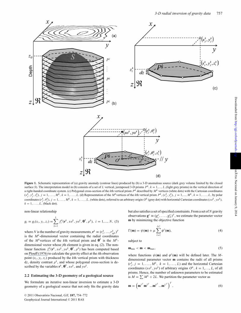
15) and the approximation of the estimated total-anomalous mass(eq. 16), we consider two extreme possibilities. In the first one, let’sassume that bi < ai , for all observation point i . In this case, thefitted gravity data underestimate the observed gravity data (Fig. 2a)and the data-misfit measure (eq. 15) can be rewritten as

s = 1

N

∑|ai | − 1

N

∑|bi |. (17)

By inserting the form of the approximate estimate of total-anomalous mass (eq. 16) into the data-misfit measure defined byeq. (15), we have the first relationship between the data-misfit mea-sure and the estimated total-anomalous mass, that is,

mt ≈ κ∑

|ai | − (Nκ)s. (18)

The above equation shows a linear relationship between the esti-mated total-anomalous mass mt and the data-misfit measure s witha negative angular coefficient. Hence, mt increases as s decreases.

In the second possibility, let us assume that bi > ai , for allobservation point i . In this case, the fitted gravity data overestimatethe observed gravity data (Fig. 2b) and the data-misfit measure (eq.15) can be rewritten as

s = 1

N

∑|bi | − 1

N

∑|ai |. (19)

By inserting the form of the approximate estimate of total-anomalous mass (eq. 16) into the data-misfit measure defined byeq. (19), we have the second relationship between the data-misfitmeasure and the estimated total-anomalous mass, that is,

mt ≈ κ∑

|ai | + (Nκ)s. (20)

The above equation shows a second linear relationship betweenthe estimated total-anomalous mass mt and the data-misfit mea-sure s with a positive angular coefficient. Hence, mt increases withincreasing s.

Note that the deduced relationships between the estimated total-anomalous mass (mt ) and the data-misfit measure (s) can be approx-imated as straight lines (eqs 18 and 20). These two straight linesintercept each other if and only if s is equal to zero. In this case, theobserved gravity data are perfectly fitted (Fig. 2c) and the estimatedtotal-anomalous mass (mt ) is approximately equal to the computedtotal-anomalous mass MT from the observed gravity data, that is,

mt ≈ κ∑

|ai | ≈ 1

2πγ

∑go

i dsi ≈ MT . (21)

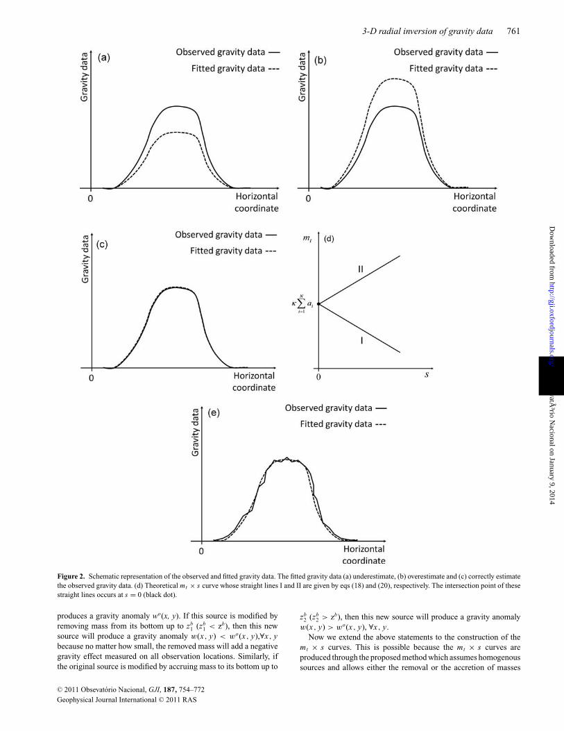
Fig. 2d shows a schematic representation on the plane mt ×s of thetheoretical straight lines I and II given by eqs 18 and 20, respectively.The intersection point of these straight lines is indicated by a blackdot, in Fig. 2(d). The graph shown in Fig. 2(d) will be referred to astheoretical mt × s curve.

3.2 Departure from the predicted relationship between thedata-misfit measure s and the estimated total-anomalousmass mt in the neighbourhood of s = 0

We have deduced two linear relationships (eqs 18 and 20) betweenthe data-misfit measure (s) and the estimated total-anomalous mass(mt ) given a stable parameter estimate m. We have also deducedthat the intersection point of these straight lines occurs when s isexactly equal to zero. In this section, we analyse the departure of theintersection point of the straight lines from s = 0, and the departureof the relationship between mt and s from a straight line in theneighbourhood of s = 0.

Let q be a non-negative number representing the smallest data-misfit value still fitting the data. If q is equal to zero the intersectionpoint of the straight lines (eqs 18 and 20) occurs at s = 0; otherwiseit departs from s = 0. Three factors contribute to this departure.The first one is the presence of noise in data. The second one isthe decrease of the gravity data power to resolve very deep source’sbottons. The third factor is the inadequacy of the interpretationmodel to retrieve the geological body. Then, if q is different fromzero, eq. (15) becomes

s = 1

N

∑|(go

i dsi ) − (gi dsi )| = 1

N

∑|ai − bi | + q. (22)

Consequently, the two linear relationships between s and mt givenby eqs (18) and (20) will be modified to

mt ≈ κ∑

|ai | − (Nκ)s + (Nκ)q, (23)

and

mt ≈ κ∑

|ai | + (Nκ)s − (Nκ)q, (24)

respectively. In this case, the intersection point of these straightlines (eqs 23 and 24) occurs at s = q. It will, therefore, be displacedtowards the positive s-axis when s > 0.

In the neighbourhood of the point s = q, the relationship betweenmt and s will depart from the predicted straight lines (eqs 18 and20) because of the presence of noise in data and of the inadequacyof the interpretation model to retrieve the geological body leadingto violation of conditions ai < bi and ai > bi , for all observationpoints i (Fig. 2e). These conditions are necessary to guarantee thestraight line behaviour described by eqs 15 and 18.

3.3 Practical procedure to determine the true (orminimum) depth to the bottom of the source through themt × s curve

To determine the true (or minimum) depth to the source’s bottom,we first need to understand the relationship between the mt × scurve with the maximum depth of the interpretation model (zmax,eq. 12) and the true (or minimum) depth to the source’s bottom.This approach is valid only if the gravity anomaly is caused by anisolated body with a homogeneous density contrast with the hostrocks and having a known depth to the top.

First, consider the following theoretical statements. Assume thata homogeneous source with maximum depth to the bottom at zb

C© 2011 Obsevatorio Nacional, GJI, 187, 754–772

Geophysical Journal International C© 2011 RAS

at ObservatÃ

³rio Nacional on January 9, 2014

http://gji.oxfordjournals.org/D

ownloaded from

3-D radial inversion of gravity data 761

Figure 2. Schematic representation of the observed and fitted gravity data. The fitted gravity data (a) underestimate, (b) overestimate and (c) correctly estimatethe observed gravity data. (d) Theoretical mt × s curve whose straight lines I and II are given by eqs (18) and (20), respectively. The intersection point of thesestraight lines occurs at s = 0 (black dot).

produces a gravity anomaly wo(x, y). If this source is modified byremoving mass from its bottom up to zb

1 (zb1 < zb), then this new

source will produce a gravity anomaly w(x, y) < wo(x, y),∀x, ybecause no matter how small, the removed mass will add a negativegravity effect measured on all observation locations. Similarly, ifthe original source is modified by accruing mass to its bottom up to

zb2 (zb

2 > zb), then this new source will produce a gravity anomalyw(x, y) > wo(x, y), ∀x, y.

Now we extend the above statements to the construction of themt × s curves. This is possible because the mt × s curves areproduced through the proposed method which assumes homogenoussources and allows either the removal or the accretion of masses

C© 2011 Obsevatorio Nacional, GJI, 187, 754–772

Geophysical Journal International C© 2011 RAS

at ObservatÃ

³rio Nacional on January 9, 2014

http://gji.oxfordjournals.org/D

ownloaded from

762 V. C. Oliveira, Jr, V. C. F. Barbosa and J. B. C. Silva

at the bottom of different tentative solutions simply by definingthe maximum depth, zmax, of the interpretation model. If zmax issmaller than the true depth to the bottom of the source, the fittedgravity data (produced by a solution using the proposed method)underestimate the observed gravity data (as shown in Fig. 2a) andlead to the theoretical straight line I approximation (Fig. 2d) on themt × s plane. Conversely, if zmax is greater than the true depth to thebottom of the source, the fitted gravity data (produced by a solutionusing the proposed method) overestimate the observed gravity data(Fig. 2b) and lead to the theoretical straight line II approximation(Fig. 2d) on the mt × s plane. Finally, if zmax coincides with the truedepth to the bottom of the source, the fitted gravity data (producedby a solution using the proposed method) are approximately equal tothe observed gravity data (Fig. 2c) and a minimum value of the data-misfit measure s (such as the one shown schematically by a black dotin Fig. 2d), is expected. In this way, by varying the maximum depthof the interpretation model (zmax, eq. 12) we construct an observedmt × s curve similar to the theoretical mt × s curve (Fig. 2d). Thetentative value for zmax producing the smallest data-misfit measures on the observed mt × s curve is an optimum estimate of the true(or minimum) depth to the bottom of the source.

Here, we do not compute the estimated total-anomalous massmt by eqs (14) or (16). Rather, it is computed from the stableparameter estimates m (see the Section 2.3). So, by assuming thecorrect knowledge of the density contrast between the geologicalsource and the host rock, we first calculate the area of the estimatedhorizontal section of the kth vertical prism by computing one half ofthe magnitude of the cross product between two estimated adjacentradius,

ak = 1

2

[(xk

Mk − xok) (

yk1 − yok

) − (xk

1 − xok) (

ykMk − yok

)]1/2 +Mk−1∑

j=1

1

2

[(xk

j − xok) (

ykj+1 − yok

) − (xk

j+1 − xok) (

ykj − yok

)]1/2,

(25)

where xkj and yk

j , i = 1 . . . Mk , are the horizontal Cartesian coor-dinates of the Mk vertices, (white dots in Fig. 1d) obtained fromthe estimated radii of the Mk vertices of the kth vertical prism andxok and yok are the estimated horizontal Cartesian coordinates ofthe kth arbitrary origin Ok (grey dot in Fig. 1d). Then, the exactexpression of the estimated total-anomalous mass is written as

mt = dzL∑

k=1

ρkak . (26)

The practical procedure to construct the observed mt × s curveis as follows. First, we assign a small value to zmax that defines theinitial interpretation model. Then, we compute the stable estimatedsolution m (see Section 2.3) whose j th element is given by eq. (10).Next, we compute the fitted gravity data produced by m that al-lows computing the data-misfit measure s(eq. 15) and the estimatedtotal-anomalous mass mt (eq. 26). Finally, we plot mt against s,producing the first point of the observed mt × s curve. We repeatthis procedure for increasingly larger values of maximum depthszmax of the interpretation model.

3.4 Illustration of the practical procedure to determine thetrue (or minimum) depth to the bottom of the sourcethrough the mt × s curve

We illustrate how the true (or minimum) depth to the bottom of thesource can be estimated from the observed mt × s curve. To do

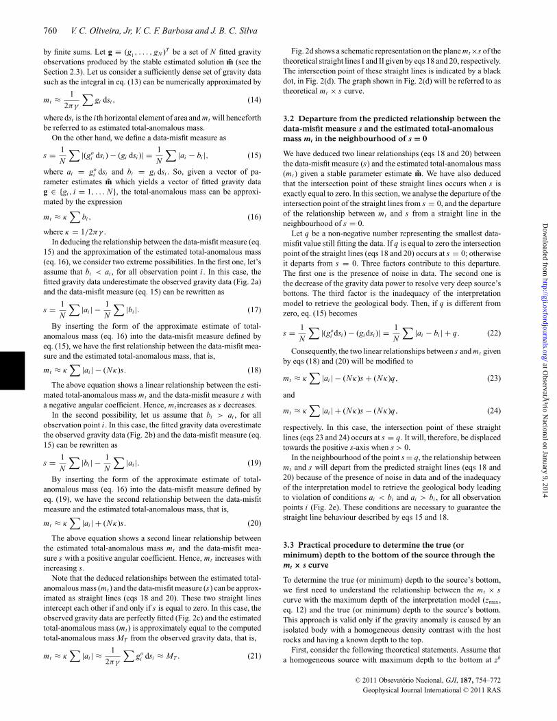
this, we simulated three outcropping dipping volcanic ducts witha density contrast ρ of 0.5 g cm–3 relative to the background anddiffering from each other by their maximum depth to the bottom.The first one is a shallow-bottomed dipping duct which attainsa maximum bottom depth of 3 km (Figs 3a–c red prisms). Thesecond simulation consists of a middle-bottomed dipping duct withbottom depth of 6 km (not shown). The third simulation involves adeep-bottomed dipping duct whose maximum bottom depth is 9 kmFigs 4a–c in red prisms). For each simulation, we computed, on theplane z = 0 km, the theoretical noise-free (not shown) and the noise-corrupted gravity data. Figs 3(a)–(c) and 4(a)–(c) show, in half-tonemaps, the noise-corrupted gravity data produced, respectively, byshallow- and deep-bottomed dipping volcanic ducts.

In all inversions, we set zo = 0 km because we simulated out-cropping dipping volcanic ducts and assumed that the depths tothe tops of the interpretation models coincide with the actual topsof the sources. To all interpretation models we set an ensemble ofL = 5 prisms, all of them with the same density contrast and thesame number of polygon vertices that describe the horizontal cross-sections. Specifically, to all prisms we set ρk = ρ = 0.5 g cm–3

and Mk = 4, for all k, k = 1,..., L . We used all the constrainingfunctions described in the Section 2, except for the third constraint(named source’s outcrop constraint, see eq. 9c).

For each simulated test, we followed the same practical proceduredescribed in the Section 3.3, but built two sets of observed mt × scurves. The first one is obtained by using the noise-free data (Fig. 5a)and second set of mt × s curves is obtained by using the noise-corrupted data (Fig. 5b). Each mt × s curve is composed by 11estimated values of mt and s, each one associated with a fixedmaximum depth zmax of the interpretation model, in which the valueof zmax varies from 1 km to 11 km by steps of 1 km. This step impliesthat the uncertainty in the estimated true (or minimum) depth to thebottom of the source is at most ±0.5 km. Fig. 5 shows the observedmt × s curves obtained for the three simulated tests where the dotscorrespond to different values of maximum depths zmax assumedfor the interpretation models.

Although the observed mt × s curves (Fig. 5) are different fromthe theoretical behaviour of the mt × s curve (Fig. 2d), they showtwo asymptotic linear relationships between the estimated total-anomalous mass mt and the data-misfit measure s, one with a nega-tive and the other with a positive angular coefficient, in accordancewith the theoretical results given by eqs (18) and (20), respectively.

In the case of the shallow-bottomed dipping duct, the minima ofs are very well defined in the observed mt × s curves, shown in bluelines, both for noise-free (Fig. 5a) and noise-corrupted (Fig. 5b)data. These minima are well defined because the gravity anomalyproduced by this shallow-bottomed source is able to estimate, underthe imposed constraints, the true maximum depth of the source pro-ducing the minimum of s. According to the theoretical derivationpresented in Section 3.1, the tentative value for the maximum depthzmax producing the minimum of the data-misfit measure s (see theblue lines in Fig. 5) is the best estimate of the true depth to thebottom of the simulated shallow-bottomed dipping duct, both fornoise-free and noise-corrupted data. The best estimate of the truedepth to the bottom of this source is zmax = 3 ± 0.5 km which agreeswith the true one. Fig. 3(b) shows that the estimated 3-D geometryof the source (blue prisms) using the maximum depth zmax = 3 kmrecovers very well the geometry of the true shallow-bottomed dip-ping duct. The corresponding fitted anomaly is displayed in Fig. 3(b)in dashed black lines. Figs 3(a) and (c) show the estimated 3-D ge-ometries of the source (blue prisms) using smaller (zmax = 2 km)or larger (zmax = 4 km) maximum depth to the bottom zmax of the

C© 2011 Obsevatorio Nacional, GJI, 187, 754–772

Geophysical Journal International C© 2011 RAS

at ObservatÃ

³rio Nacional on January 9, 2014

http://gji.oxfordjournals.org/D

ownloaded from

3-D radial inversion of gravity data 763

Figure 3. Synthetic data application produced by a simulated outcropping dipping volcanic duct. Perspective views of the true (red prisms) and estimated(blue prisms) shallow-bottomed dipping duct; the latter is obtained by inverting the noise-corrupted gravity data (half-tone contour map) and assuming aninterpretation model with maximum bottom depths zmax (a) smaller (2 km); (b) equal (3 km) and (c) larger (4 km) than the true one. The corresponding fittedgravity anomalies produced by the estimated sources (blue prisms in a–c) are shown in dashed black lines in the contour maps (a)–(c).

interpretation models relative to the true one. In this case, neitherestimated 3-D geometry of the sources (blue prisms in Figs 3a andc) recover the true geometry of the shallow-bottomed dipping duct(red prisms), even though both solutions fit the gravity observations(dashed black lines in Figs 3a and c). In the case of the deep-bottomed dipping duct, the minimum of s is reasonable, defined bythe mt × s curve obtained for noise-free data (green line in Fig. 5a).On the other hand, the noise-corrupted gravity data produced bythe deep-bottomed dipping duct do not have enough resolution todefine the smallest value of s in the mt × s curve (green line inFig. 5b) and, consequently, to produce reliable estimates of the truemaximum depth of the source. So, the ambiguous smallest valueof s in the mt × s curve (green line in Fig. 5b) indicates the im-possibility of determining the true maximum depth of the source.In this case, this mt × s curve can be used to estimate, at most, alower bound (zmax = 6 ± 0.5 km) for the maximum depth of thesource. The loss of resolution of the gravity data with depth leadsto the impossibility of retrieving the 3-D geometry of the deepestpart of the true source (red prisms) as shown in Figs 4(a)–(c); how-ever, the shallowest part of the true source geometry is reasonablyretrieved. In Figs 4(a)–(c) the maximum depth zmax, assumed forthe interpretation models, are, respectively, smaller (zmax = 8 km),equal (zmax = 9 km) and larger (zmax = 10 km) than the true one.Neither estimated geometries (blue prisms in Figs 4a–c) perfectly

recovered the true dipping volcanic duct (red prisms in Figs 4a–c),even though all of them fit the gravity data (dashed black lines inFigs 4a–c) and are stable. These unsatisfactory results, even usingan interpretation model whose maximum depth of the interpretationmodel coincides with the true one (Fig. 4b), are expected becauseof the inevitable loss of data resolution with depth. The gravity datalack the necessary in depth resolution and this low resolution makesit impractical to estimate the deepest portion of the source withoutusing prior information (e.g. Silva Dias et al. 2009).

Some striking features in Fig. 5 deserve attention. First, the theo-retical linear behaviour of the mt × s curve at its extremities, shownschematically in Fig. 2(d) has been confirmed numerically. Besides,we have also confirmed numerically that the smallest value of thedata-misfit measure in the observed mt × s curve occurs close tos = 0 in the case of noise-free data (Fig. 5a); in the case of noise-corrupted data, the minimum of s is displaced towards the positives-axis (Fig. 5b). Finally, our new criterion for determining the true(or minimum) depth to the bottom of the source is theoreticallysound. This criterion determines the true depth to the bottom ofthe source if the gravity anomaly has enough resolution to resolveit. A better resolution of the data is inferred from inspecting theexistence of a well-defined minimum of s on the observed mt × scurve, such as those produced by the shallow- and middle-bottomeddipping ducts (blue and red lines in Fig. 5). Otherwise, if the data

C© 2011 Obsevatorio Nacional, GJI, 187, 754–772

Geophysical Journal International C© 2011 RAS

at ObservatÃ

³rio Nacional on January 9, 2014

http://gji.oxfordjournals.org/D

ownloaded from

764 V. C. Oliveira, Jr, V. C. F. Barbosa and J. B. C. Silva

Figure 4. Synthetic data application produced by a simulated outcropping dipping duct. Perspective views of the true (red prisms) and estimated (blue prisms)deep-bottomed dipping duct; the latter is obtained by inverting the noise-corrupted gravity data (half-tone contour map) and assuming an interpretation modelwith maximum bottom depths zmax(a) smaller (8 km); (b) equal (9 km) and (c) larger (10 km) than the true one. The corresponding fitted gravity anomaliesproduced by the estimated sources (blue prisms in a–c) are shown in dashed black lines in the contour maps (a)–(c).

do not have enough resolution, our criterion can determine, at most,the minimum depth to the bottom of the source and retrieve thegeometry of part of the true source above this determined minimumdepth. This aspect is illustrated in Fig. 4 whose shallowest part ofthe estimated geometries (blue prisms above the depth of 6 km)coincide with the upper portion of the true source (red prisms). Apoor resolution of the data is evidenced by an observed mt ×s curveexhibiting an ill-defined minimum value of s, such as the one shownby the green line in Fig. 5(b).

4 . A P P L I C AT I O N T O S Y N T H E T I C DATA

We present two applications using synthetic gravity data simulatingtwo different isolated geological sources with known density con-trasts. In the first one we simulated an outcropping granitic plutonemplaced in homogeneous country rocks. In the second application

we simulated an outcropping dipping intrusive body having variabledips and strikes and exhibiting a complex form.

In all applications the irregularly distributed gravity data werecomputed on plane z = 0 km and contaminated with different pseu-dorandom Gaussian noise sequences with zero mean and a standarddeviation as specified below. In each application we adopted thesame practical procedure described in the Section 3.3 to obtain notonly a stable solution that fits the data, but also to determine thetrue (or minimum) depth to the bottom of the source.

In all inversions, we set zo = 0 km because we simulated out-cropping bodies and assumed that the depths to the tops of theinterpretation models coincide with the actual tops of the sources.We established that all prisms defining the interpretation modelhave the same density contrast and the same number of the verticesof the polygons which describe their horizontal cross-sections. Wealso assumed the correct density contrast between the source andthe host rocks.

C© 2011 Obsevatorio Nacional, GJI, 187, 754–772

Geophysical Journal International C© 2011 RAS

at ObservatÃ

³rio Nacional on January 9, 2014

http://gji.oxfordjournals.org/D

ownloaded from

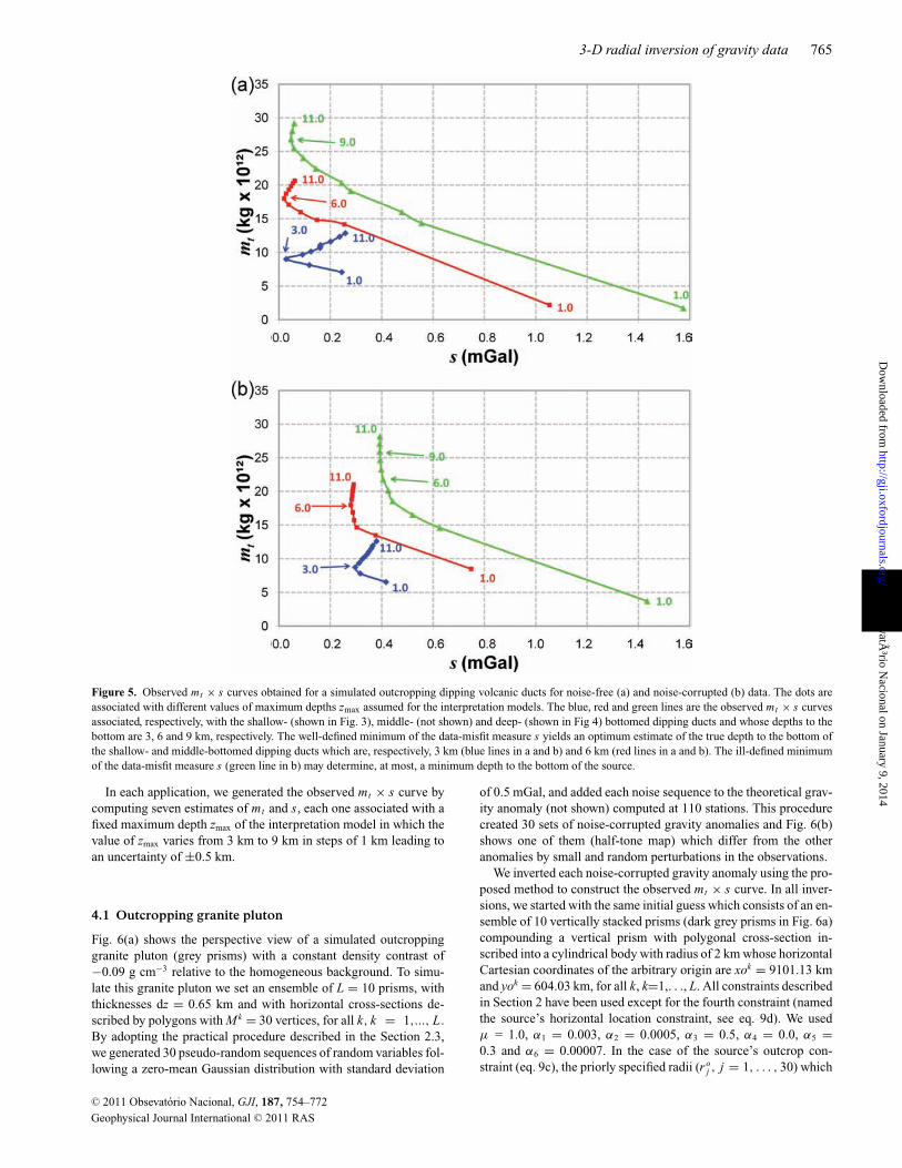
3-D radial inversion of gravity data 765

Figure 5. Observed mt × s curves obtained for a simulated outcropping dipping volcanic ducts for noise-free (a) and noise-corrupted (b) data. The dots areassociated with different values of maximum depths zmax assumed for the interpretation models. The blue, red and green lines are the observed mt × s curvesassociated, respectively, with the shallow- (shown in Fig. 3), middle- (not shown) and deep- (shown in Fig 4) bottomed dipping ducts and whose depths to thebottom are 3, 6 and 9 km, respectively. The well-defined minimum of the data-misfit measure s yields an optimum estimate of the true depth to the bottom ofthe shallow- and middle-bottomed dipping ducts which are, respectively, 3 km (blue lines in a and b) and 6 km (red lines in a and b). The ill-defined minimumof the data-misfit measure s (green line in b) may determine, at most, a minimum depth to the bottom of the source.

In each application, we generated the observed mt × s curve bycomputing seven estimates of mt and s, each one associated with afixed maximum depth zmax of the interpretation model in which thevalue of zmax varies from 3 km to 9 km in steps of 1 km leading toan uncertainty of ±0.5 km.

4.1 Outcropping granite pluton

Fig. 6(a) shows the perspective view of a simulated outcroppinggranite pluton (grey prisms) with a constant density contrast of−0.09 g cm−3 relative to the homogeneous background. To simu-late this granite pluton we set an ensemble of L = 10 prisms, withthicknesses dz = 0.65 km and with horizontal cross-sections de-scribed by polygons with Mk = 30 vertices, for all k, k = 1,..., L .By adopting the practical procedure described in the Section 2.3,we generated 30 pseudo-random sequences of random variables fol-lowing a zero-mean Gaussian distribution with standard deviation

of 0.5 mGal, and added each noise sequence to the theoretical grav-ity anomaly (not shown) computed at 110 stations. This procedurecreated 30 sets of noise-corrupted gravity anomalies and Fig. 6(b)shows one of them (half-tone map) which differ from the otheranomalies by small and random perturbations in the observations.

We inverted each noise-corrupted gravity anomaly using the pro-posed method to construct the observed mt × s curve. In all inver-sions, we started with the same initial guess which consists of an en-semble of 10 vertically stacked prisms (dark grey prisms in Fig. 6a)compounding a vertical prism with polygonal cross-section in-scribed into a cylindrical body with radius of 2 km whose horizontalCartesian coordinates of the arbitrary origin are xok = 9101.13 kmand yok = 604.03 km, for all k, k=1,. . ., L. All constraints describedin Section 2 have been used except for the fourth constraint (namedthe source’s horizontal location constraint, see eq. 9d). We usedμ = 1.0, α1 = 0.003, α2 = 0.0005, α3 = 0.5, α4 = 0.0, α5 =0.3 and α6 = 0.00007. In the case of the source’s outcrop con-straint (eq. 9c), the priorly specified radii (ro

j , j = 1, . . . , 30) which

C© 2011 Obsevatorio Nacional, GJI, 187, 754–772

Geophysical Journal International C© 2011 RAS

at ObservatÃ

³rio Nacional on January 9, 2014

http://gji.oxfordjournals.org/D

ownloaded from

766 V. C. Oliveira, Jr, V. C. F. Barbosa and J. B. C. Silva

Figure 6. Synthetic data application produced by a simulated outcropping granite. (a) Perspective views of the simulated outcropping granite (light greyprisms) and the initial guess (dark grey prisms) used in all inversions. (b) Noise-corrupted gravity anomaly (half-tone contour map) produced by the graniteshown in (a) and fitted gravity anomaly (dashed black lines) produced by the solution shown in Figs 7(b) and (c) (blue prisms). The intersection between thehorizontal erosion surface and the interface separating the granite from the host rock is shown by the white line. The white cross indicates the priorly specifiedhorizontal Cartesian coordinates (xoo, yoo) used in eq. 9c.

describe the edge of the polygonal cross-section of the first verticalprism were defined by using the known outcropping interface sep-arating the granite from the host rock (white line in Fig. 6b). Thisset of priorly specified radii of the shallowest prism of the interpre-tation model will be referred to an origin whose priorly specifiedhorizontal Cartesian coordinates are xoo = 9101.13 km and yoo =604.03 km (white cross in Fig. 6b). We used xomin = 9090.0 km,xomax = 9115.0 km, yomin = 590 km, yomax = 610 km, rmin = 0 kmand rmax = 25 km for all prisms. In the inversions, the interpretationmodel consists of an ensemble of L = 10 prisms with horizontalcross-sections described by polygons with Mk = 30 vertices, forall k, k = 1,..., L . Then, the 30 estimates are used to compute thestable sample mean parameter vector m (eq. 10) that will be usedto build the mt × s curve.

Fig. 7(a) shows the observed mt × s curve where the dots cor-respond to different values of maximum depths zmax assumed forthe interpretation models. We clearly note a well-defined minimumof s on the observed mt × s curve, associated with zmax = 6 km.Because this minimum is well defined, we conclude that the gravitydata have good resolution to estimate the depth to the bottom ofthe simulated granite as 6 ± 0.5 km. Figs 7(b) and (c) show theperspective views of the estimated (blue prisms) and the true (redprisms) granites using the maximum depth zmax = 6 km. Fig. 7(d)shows a set of horizontal depth slices of the estimated (blue lines)and true (red lines) upper edges of the polygonal cross-sectionsdescribing the geometry of the granite. This inversion result showsthat the estimated 3-D body efficiently retrieves the true geometryof the granite body. The corresponding fitted anomaly is displayedin Fig. 6(b) in dashed black lines.

4.2 Outcropping dipping intrusion

We simulated an isolated outcropping dipping intrusion that is em-bedded in homogeneous rocks with a constant density contrast of0.4 g cm–3 relative to the host rocks. This body fills a simulatedopening created along a curved fracture. Fig. 8(a) displays a per-spective view of this dipping intrusion (light grey prisms) whoseshape resembles a spiral staircase. To simulate this intrusion we set

up an ensemble of L = 14 prisms, with thicknesses dz = 0.5 km andhorizontal cross-sections described by polygons with Mk = 16 ver-tices, for all k, k = 1,..., L . Here, we adopted the same proceduredescribed in the previous application. Hence, we inverted 30 sets ofnoise-corrupted gravity data obtained by adding different pseudo-random sequences of Gaussian noise, with zero mean and a standarddeviation of 0.8 mGal, to the theoretical data. Fig. 8(b) shows oneof them (half-tone map). To determine the bottom of the source andinvert the gravity anomaly aiming at estimating the 3-D geometryof the simulated intrusion, we constructed initially the mt × s curve(Section 3.3). In this way, we inverted the 30 sets of noise-corruptedgravity data by starting at the same initial guess shown in Fig. 8(a)by dark grey prisms. This initial guess has been selected on thebasis of the anomaly features and it consists of two parts. In bothparts, an ensemble of seven vertically stacked prisms compoundinga vertical prism with polygonal cross-section inscribed into a cylin-drical body with radius of 5 km. The first part is composed by theseven shallowest prisms that make up the interpretation model. Allthese prisms have the same horizontal Cartesian coordinates of thearbitrary origin, equal to xok = 51.671 km and yok = 96.453 km,k = 1,..., 7 (indicated by point A in Fig. 8b). The second part of theinitial guess is composed by the seven deepest prisms that make upthe interpretation model. All these prisms have the same horizontalCartesian coordinates of the arbitrary origin of xok = 128.156 kmand yok =65.686 km, k = 1,..., 7, (indicated by point B in Fig. 8b).The horizontal Cartesian coordinates of the arbitrary origin relatedwith the shallow- and the deep-seated cylinders were taken fromthe horizontal coordinates of, respectively, the gravity high and thesmooth gravity signal (Fig. 8b). In the previous synthetic example,we assumed the knowledge about the intersection of the erosion sur-face with the interface separating the intrusion source from the hostrock. Here, we assumed just the knowledge about the horizontal co-ordinates of the centre outcropping intrusion (eq. 9d) and assigned:xoo =38.420 km and yoo =98.121 km (white cross in Fig. 8b). Weused μ = 1.0, α1 = 0.0005, α2 = 0.005, α3 = 0.0, α4 = 0.1, α5 =0.1 and α6 = 0.00005. Hence, all constraints described in Section 2have been used, except for the third constraint (named the source’soutcrop constraint presented in eq. 9c). We used xomin = 20 km,xomax = 160 km, yomin = 10 km, yomax = 130 km, rmin = 0 km

C© 2011 Obsevatorio Nacional, GJI, 187, 754–772

Geophysical Journal International C© 2011 RAS

at ObservatÃ

³rio Nacional on January 9, 2014

http://gji.oxfordjournals.org/D

ownloaded from

3-D radial inversion of gravity data 767

Figure 7. Synthetic data application produced by a simulated outcropping granite. (a) Observed mt × s curve where the dots are associated with differentvalues of maximum depths zmax assumed for the interpretation models. The well-defined minimum value of s, which is associated with zmax = 6 km, determinesthe depth to the bottom of the simulated granite. (b) and (c) Perspective views of the true (red prisms) and estimated (blue prisms) granites; the latter is obtainedby inverting the gravity anomaly shown in Fig. 6(b) in half-tone contours and assuming an interpretation model with maximum bottom depth of 6.0 kmestimated from the mt × s curve criterion shown in (a). (d) Ensemble of horizontal depth slices of the true (red lines) and estimated (blue lines) edges of thepolygonal cross-sections describing the geometry of the granite.

and rmax = 50 km for all prisms. In the inversions, the interpretationmodel consists of an ensemble of L = 14 prisms with horizontalcross-sections described by polygons with Mk = 16 vertices, for allk, k = 1,..., L .

Fig. 9(a) shows the observed mt × s curve where the dots arerelated with the different maximum depths zmax assumed for theinterpretation models. Again, the observed mt × s curve reveals awell-defined minimum value of s, associated with zmax = 7 km, andprovides a well-resolved depth-to-bottom estimate of 7 ± 0.5 km

for the simulated outcropping dipping intrusion, coinciding withthe true depth to the bottom of this intrusion. Figs 9(b) and (c)show the perspective views of the estimated (blue prisms) and thetrue (red prisms) dipping intrusions using the maximum depth ofzmax = 7 km for the interpretation model. Fig. 9(d) shows a set ofhorizontal depth slices of the estimated (blue lines) and true (redlines) upper edges of the polygonal cross-sections describing thegeometry of the dipping intrusion. This solution shows the excellentperformance of our method in recovering the 3-D geometry of true

C© 2011 Obsevatorio Nacional, GJI, 187, 754–772

Geophysical Journal International C© 2011 RAS

at ObservatÃ

³rio Nacional on January 9, 2014

http://gji.oxfordjournals.org/D

ownloaded from

768 V. C. Oliveira, Jr, V. C. F. Barbosa and J. B. C. Silva

Figure 8. Synthetic data application produced by a simulated outcropping dipping intrusion. (a) Perspective views of the simulated dipping intrusion (lightgrey prisms) and the initial guess (dark grey prisms) used in all inversions. (b) Noise-corrupted gravity anomaly (half-tone contour map) produced by theintrusion shown in (a) and fitted gravity anomaly (dashed black lines) produced by the solution shown in Figs 9(b) and (c) (blue prisms). The white crossindicates the priorly specified horizontal Cartesian coordinates (xoo, yoo) used in eq. 9d. Points A and B define the horizontal coordinates where the two partsof the initial guess are located.

dipping intrusion resembling a spiral staircase-shaped feature. Thecorresponding fitted anomaly is shown in Fig. 8(b) in dashed blacklines.

5 . A P P L I C AT I O N T O R E A L DATA

The Archean Matsitama greenstone belt in northeastern Botswanaoccurs at the southwestern extremity of the Zimbabwe Craton(Ranganai et al. 2002; McCourt et al. 2004). Fig. 10 shows a sim-plified geological map of Matsitama, northeastern Botswana, wherethe greenstone belt from Matsitama becomes progressively maskedto the west because of the overlying Kalahari and Karoo sediments.The original gravity observations (see Reeves 1985; Silva et al.2007) indicates that greenstone rocks extend themselves westwardsand then northeastwards (open circles in Fig. 10). In this area, ashallow borehole directed to coal exploration in the sedimentarycover confirmed the presence of Precambrian ultramafic rocks.

Fig. 11 shows the residual Bouguer anomaly map (half-tone map)over the Matsitama greenstone belt. We used the same practicalprocedure described for the previous test. Hence, we produced andinverted 30 sets of noise-corrupted gravity anomalies obtained byadding different pseudorandom sequences of Gaussian noise, withzero mean and a standard deviation of 0.8 mGal, to the field data(half-tone map in Fig. 11). We stress that the only physical aim ofadding extra noise to field data is to analyse the solution stability.The final estimates are obtained with the original observations inall inversions we have started at the same initial guess and haveassumed the constant density contrast of 0.4 g cm–3 between theMatsitama intrusion and the country rocks. We also set an inter-pretation model with L = 14 prisms, with a constant density con-trast of 0.4 g cm–3 and with horizontal cross-sections describedby polygons with Mk = 16 vertices, for all k, k = 1,..., L . Then,

the 30 estimates are used to compute the stable sample mean pa-rameter vector m (eq. 10) that has been used to build the mt × scurve.

Based on the synthetic application to interpret an outcroppingdipping intrusion, shown in Section 4.2, the initial guess (not shown)consists of two ensembles of seven vertically stacked prisms, eachone consisting of a vertical prism with polygonal cross-section,inscribed into a cylindrical body with radius 5 km and with differenthorizontal coordinates of the centre. The first ensemble is composedof the seven shallowest prisms that make up the interpretation modelwith horizontal Cartesian coordinates of the arbitrary origin equalto xok =51.671 km and yok = 96.453 km, k = 1,..., 7. Thesehorizontal Cartesian coordinates (point A in Fig. 11) were chosenas the horizontal coordinates close to the gravity high. The secondensemble is composed of the seven deepest prisms that make upthe interpretation model with horizontal Cartesian coordinates ofthe arbitrary origin equal to xok =128.16 km and yok =65.69 km.These horizontal Cartesian coordinates were chosen as those locatedat the smooth gravity signal (point B in Fig. 11). The Matsitamaintrusion is in fact a shallow buried body; however, here we assumedthat this body crops out and that the knowledge about the horizontalcoordinates of its shallowest portion is xoo = 38.420 km and yoo =98.121 km (white cross in Fig. 11). Hence, all constraints describedin the Section 2 have been used except for the third constraint(named the source’s outcrop constraint; see eq. 9c) because theshallowest boundary of the intrusion is unknown. The inversioncontrol variables used in all inversions are μ = 1.0, α1 = 0.0001,α2 = 0.001, α3 = 0.0, α4 = 0.1, α5 = 0.01 and α6 = 0.00005. Weused xomin = 20 km, xomax = 160 km, yomin = 10 km, yomax =130 km, rmin = 0 km and rmax = 50 km for all prisms.

According to the criterion described in the Section 3.3 the mini-mum of s on the observed mt × s curve is associated with the true

C© 2011 Obsevatorio Nacional, GJI, 187, 754–772

Geophysical Journal International C© 2011 RAS

at ObservatÃ

³rio Nacional on January 9, 2014

http://gji.oxfordjournals.org/D

ownloaded from

3-D radial inversion of gravity data 769

Figure 9. Synthetic data application produced by a simulated outcropping dipping intrusion. (a) Observed mt × s curve where the dots are associated withdifferent values of maximum depths zmax assumed for the interpretation models. The well-defined minimum value of s, which is associated with zmax = 7 km,determines the depth to the bottom of the simulated intrusion. (b) and (c) Perspective views of the true (red prisms) and estimated (blue prisms) intrusions; thelatter is obtained by inverting the gravity anomaly shown in Fig. 8(b) in half-tone contours and assuming an interpretation model with maximum bottom depthof 7 km estimated from the mt × s curve criterion shown in (a). (d) Ensemble of horizontal depth slices of the true (red lines) and estimated (blue lines) edgesof the polygonal cross-sections describing the geometry of the dipping intrusion.

(or minimum) depth of the source, depending on whether the truesource produces a gravity anomaly that is able (or not) to resolve thesource’s bottom. We generated the observed mt × s curve by com-puting eight estimated values of mt and s, each one associated witha fixed maximum depth zmax of the interpretation model, in whichthe value of zmax varies from 3 km to 10 km in steps of 1 km leadingto an uncertainty of ±0.5 km. Fig. 12(a) shows that the minimum ofs is associated with a depth to the bottom of 8.0 ± 0.5 km. Becausethis mt × s curve shows a well-defined minimum of s, it suggeststhat the gravity data are able to resolve the depth-to-bottom estimateof the Matsitama intrusion. The estimated source fits acceptably thegravity anomaly (dashed black lines in Fig. 11) and retrieves a dip-ping intrusion with variable dips and strikes with bottom’s depthof 8 ± 0.5 km (Figs 12b and c). This result is consistent with theavailable geological information reported by Reeves (1985) that

the greenstone rocks extend themselves westwards. However, theanomaly fit obtained in the Matsitama application (dashed blacklines in Figs 12b and c) is worse than that obtained in the syntheticapplications. This poorer fitting yielded in Matsitama applicationmay be related to possible violations of premises assumed by ourmethod. The presence of multiple sources, for example, giving riseto an interfering gravity anomaly, may produce a poor data fit. An-other possibility is that we inverted a truncated gravity anomaly(half-tone map in Fig. 11).

6 . C O N C LU S I O N S

We have proposed a gravity-inversion method and the mt × scurve criterion to estimate the 3-D geometry of isolated sources,

C© 2011 Obsevatorio Nacional, GJI, 187, 754–772

Geophysical Journal International C© 2011 RAS

at ObservatÃ

³rio Nacional on January 9, 2014

http://gji.oxfordjournals.org/D

ownloaded from

770 V. C. Oliveira, Jr, V. C. F. Barbosa and J. B. C. Silva

Figure 10. Simplified geological map of Matsitama, northeastern Botswana, displaying igneous rocks (B) and its extension (open circles), inferred by theinspection of the original Bouguer anomaly map (not shown). After Reeves (1985).

Figure 11. Matsitama greenstone rocks (Botswana). Bouguer anomaly map(half-tone contour map) from the Matsitama area corrected for gravity effectsproduced by the Moho. The dashed black lines show the fitted Bougueranomaly produced by the corresponding estimated source in Fig. 12(b)and (c). The white cross indicates the prior specified horizontal Cartesiancoordinates (xoo, yoo) used in eq. 9d. Points A and B define the horizontalcoordinates where the two parts of the initial guess are located.

assuming the knowledge about the density contrast and about thedepth to the source’s top. Our method implicitly introduces ho-mogeneity and compactness constraints through the interpretationmodel which consists of a set of 3-D vertical, juxtaposed prismsin the vertical direction, whose thicknesses and density contrastsare known and whose horizontal cross-sections are described by anarbitrary and unknown polygon. The geometry of the 3-D source isdefined by estimating the geometry of the set of polygons definingthe horizontal sections of vertically stacked prisms. The polygonvertices of each prism are described by polar coordinates with an

unknown origin inside the top of the prism. Our method estimatesthe radii associated with polygon vertices for a fixed number ofequally spaced angles spanning the interval between 0o and 360o,and the horizontal Cartesian coordinates of the arbitrary origin. Toguarantee a stable solution which fits the gravity data, our methodimposes constraints on the source shape. Although the estimatedsource shape is stable and yields an acceptable anomaly fit, it de-pends on the maximum depth assumed by the interpretation model.

We have proposed a new criterion to reduce the class of possiblesolutions compatible with the gravity anomaly and to determine theoptimum depth-to-bottom estimate of the source. This criterion isbased on the estimated data-misfit measure (s) and on the estimatedtotal-anomalous mass (mt ). These estimates are computed alongsuccessive inversions by using different tentative maximum depthsfor the interpretation model. The tentative value for the maximumdepth producing the smallest data-misfit measure is the best estimateof the bottom’s depth of the source and it is chosen by means of amt × s curve for the range of different tentative maximum depths.This criterion was extensively tested with synthetic data. In the casethat a minimum of s on the mt × s curve is well defined, the methodalways produced correct estimates of the bottom’s depth of thesource and recovered the 3-D geometry of the source. Conversely,if the smallest value of s on the mt ×s curve is ill-defined, the mt ×scurve criterion may only determine a minimum source’s depth tothe bottom. Even in this case, our inversion method retrieves theupper portion of the source above the lower bound estimated for thesource’s depth to the bottom.

This inversion method and the mt × s curve criterion have beenapplied to both synthetic and field data sets showing their effi-ciency in retrieving the geometry of 3-D sources, even in the caseof a complex simulated body with variable dips and strikes thatintrudes a curved fracture, a unique characteristic among most 3-Dgravity-inversion methods. This inversion method has the advan-tage of requiring no explicit assumption about the geometry ofthe anomalous source and, because the interpretation model con-sists of homogeneous prisms, no constraints favouring homogeneityand compactness are required, which makes it operationally simple.However, the method is restricted to isolated sources with knowndepth to the top and density contrast. When these assumptions holdand the gravity data have sufficient resolution, the inversion methodand the mt ×s curve criterion produce good estimates of the geome-try of the anomalous source. Otherwise, the estimated solution may

C© 2011 Obsevatorio Nacional, GJI, 187, 754–772

Geophysical Journal International C© 2011 RAS

at ObservatÃ

³rio Nacional on January 9, 2014

http://gji.oxfordjournals.org/D

ownloaded from

3-D radial inversion of gravity data 771

Figure 12. Matsitama greenstone rocks (Botswana). (a) Observed mt × s curve where the dots are associated with different values of maximum depths zmax

assumed for the interpretation models. The well-defined minimum value of s, which is associated with zmax = 8 km, determines the depth to the bottom ofthe Matsitama intrusion. (b) and (c) Perspective views of the initial guess (dark grey prisms) used in all inversions and the estimated 3-D geometry of thegreenstone belt (light grey prisms) obtained by inverting the gravity anomaly shown in Fig. 11 in half-tone contours.

produce a poor anomaly fit and may fail to retrieve the geometry ofthe gravity source.

Our method can be extended to invert interfering gravity anoma-lies produced by multiple sources. Additionally, the 3-D radial in-version can be extended to invert magnetic data and the gradientcomponents of gravity and magnetic data.

A C K N OW L E D G M E N T S

We thank an anonymous editor and two reviewers Horst Holsteinand Fabio Caratori Tontini for their valuable criticism. The au-thors were supported in this research by fellowships (VCF andJBCS) from Conselho Nacional de Desenvolvimento Cientıfico eTecnologico (CNPq) and scholarship (VCO Jr) from Coordenacaode Aperfeicoamento de Pessoal de Nıvel Superior (CAPES), Brazil.

R E F E R E N C E S

Barbosa, V.C.F. & Silva, J.B.C., 1994. Generalized compact gravity inver-sion, Geophysics, 59, 57–68.

Barbosa, V.C.F. & Silva, J.B.C., 2006. Interactive 2D magnetic inversion: atool for aiding forward modeling and testing geologic hypotheses, Geo-physics, 71, L43–L50.

Barbosa, V.C.F., Silva, J.B.C. & Medeiros, W.E., 1999a. Stable inversionof gravity anomalies of sedimentary basins with nonsmooth basementreliefs and arbitrary density contrast variations, Geophysics, 64, 754–764.

Barbosa, V.C.F., Silva, J.B.C. & Medeiros, W.E., 1999b. Gravity inversionof a discontinuous relief stabilized by weighted smoothness constraintson depth, Geophysics, 64, 1429–1437.

Barbosa, V.C.F., Silva, J.B.C. & Medeiros, W.E., 2002. Practical applicationsof uniqueness theorems in gravimetry, part II: pragmatic incorporation ofconcrete geologic information, Geophysics, 67, 795–800.

Bertete-Aguirre, H., Cherkaev, E. & Oristaglio, M., 2002. Non-smoothgravity problem with total variation penalization functional, Geophys. J.Int., 149, 499–507.

Blakely, R.J., 1995. Potential Theory in Gravity and Magnetic Applications,Cambridge University Press, Cambridge.

Calcagno, P., Chiles, J.P., Courrioux, G. & Guillen, A., 2008. Geologicalmodelling from field data and geological knowledge, part I. Modellingmethod coupling 3D potential-field interpolation and geological rules,Phys. Earth planet. Inter., 171, 147–157.

C© 2011 Obsevatorio Nacional, GJI, 187, 754–772

Geophysical Journal International C© 2011 RAS

at ObservatÃ

³rio Nacional on January 9, 2014

http://gji.oxfordjournals.org/D

ownloaded from

772 V. C. Oliveira, Jr, V. C. F. Barbosa and J. B. C. Silva

Guillen, A. & Menichetti, V., 1984. Gravity and magnetic inversion withminimization of a specific functional, Geophysics, 49, 1354–1360.

Hammer, S., 1945. Estimating ore masses in gravity prospecting, Geo-physics, 10, 50–62.

LaFehr, T.R., 1965. The estimation of the total amount of anomalous massby Gauss’s theorem, J. geophys. Res., 70, 1911–1919.

Last, B.J. & Kubik, K., 1983. Compact gravity inversion, Geophysics, 48,713–721.

Luo, X., 2010. Constraining the shape of a gravity anomalous body us-ing reversible jump Markov chain Monte Carlo, Geophys. J. Int., 180,1067–1089.

Marquardt, D.W., 1963. An algorithm for least-squares estimation of non-linear parameters, J. Soc. Ind. appl. Math., 2, 601–612.

McCourt, S., Kampunzu, A.B., Bagai, Z. & Armstrong, R.A., 2004. Thecrustal architecture of Archaean terranes in Northeastern Botswana, S.Afr. J. Geol., 107, 147–158.

Moraes, R.A.V. & Hansen, R.O., 2001. Constrained inversion of gravityfields for complex 3D structures, Geophysics, 66, 501–510.

Plouff, D., 1976. Gravity and magnetic fields of polygonal prisms andapplication to magnetic terrain corrections, Geophysics, 41, 727–741.

Portniaguine, O. & M.S. Zhdanov, 1999, Focusing geophysical inversionimages, Geophysics, 64, 874–887.

Ranganai, R.T., Kampunzu, A.B., Atekwana, E.A., Paya, B.K., King, J.G.,Koosimile, D.I. & Stettler, E.H., 2002. Gravity evidence for a larger

Limpopo belt in southern Africa and geodynamic implications. Geophys.J. Int., 149, F9–F14.

Reeves, C.V., 1985, The Kalahari Desert, central southern Africa: a casehistory of regional gravity and magnetic exploration, in, The Utility ofRegional Gravity and Magnetic Anomaly Maps, pp. 144–153, ed. Hinze,W.J., SEG.

Silva, J.B.C. & Barbosa, V.C.F., 2004. Generalized radial inversion of 2Dpotential field data, Geophysics, 69, 1405–1413.

Silva, J.B.C. & Barbosa, V.C.F., 2006. Interactive gravity inversion, Geo-physics, 71, J1–J9.

Silva, J.B.C., Medeiros, W.E. & Barbosa, V.C.F., 2001a. Potential field in-version: choosing the appropriate technique to solve a geologic problem,Geophysics, 66, 511–520.

Silva, J.B.C., Medeiros, W.E. & Barbosa, V.C.F., 2001b. Pitfalls in nonlinearinversion, Pure appl. Geophys., 158, 945–964.

Silva, J.B.C., Oliveira, F.S., Barbosa, V.C.F. & Campos Velho, H.F., 2007.Apparent-density mapping using entropic regularization, Geophysics, 72,I51–I60.

Silva Dias, F.J.S., Barbosa, V.C.F. & Silva, J.B.C., 2009. 3D gravity inversionthrough an adaptive learning procedure, Geophysics, 74, I9–I21.

Tikhonov, A.N. & Arsenin, V.Y., 1977. Solutions of Ill-Posed Problems,W. H. Winston & Sons, Washington, DC.

Wildman R.A. & Gazonas, G.A., 2009. Gravitational and magnetic anomalyinversion using a tree-based geometry representation, Geophysics, 74,I23–I35.

C© 2011 Obsevatorio Nacional, GJI, 187, 754–772

Geophysical Journal International C© 2011 RAS

at ObservatÃ

³rio Nacional on January 9, 2014

http://gji.oxfordjournals.org/D

ownloaded from