Green supplier selection using multi-criterion decision making ...

Contents lists available at ScienceDirect

Computers & Industrial Engineering

journal homepage: www.elsevier.com/locate/caie

Green supplier selection using multi-criterion decision making under fuzzyenvironment: A case study in automotive industryShubham Guptaa, Umang Sonia,⁎, Girish KumarbaNetaji Subhas Institute of Technology, University of Delhi, IndiabDelhi Technological University, New Delhi, India

A R T I C L E I N F O

Keywords:AHPTOPSISMABACWASPASFuzzy set theoryConsistency testSensitivity analysis

A B S T R A C T

In the past few decades, it has been widely observed that environmental awareness is continuously increasingamong people, stakeholders, and governments. However, rigorous environmental rules and policies pushedorganizations to accept affirmative changes like green supply chain management practices in their processes ofthe supply chain. Selection of green supplier is a tedious task and comprises a lot of challenges starting fromevaluation to their final selection, which is experienced by supplier management professionals. The developmentand implementation of practical decision-making tools that seek to address these challenges are rapidly evolving.In the present work, the evaluation of a set of suppliers is primarily based on both conventional and environ-mental criteria. This work proposes a multi-criteria decision making (MCDM) based framework that is used toevaluate green supplier selection by using an integrated fuzzy Analytical Hierarchy Process (AHP) with the otherthree techniques namely MABAC (“Multi-Attributive Border Approximation Area Comparison”), WASPAS(“Weighted Aggregated Sum-Product Assessment”) and TOPSIS (“Technique for order preference by similarity toideal Solution”). Initially, six green supplier selection environmental criteria (Environmental managementsystem, green image, staff environment training, eco-design, pollution control, and resource consumption) andthree conventional criteria (price, quality and service level) have been identified through literature review andexpert’s opinions to employ MCDM approach. A real-world case study of the automotive industry in India isdeliberated to exhibit the proposed framework applicability. From AHP findings, ‘Environment managementsystem’, ‘Pollution control’, ‘Quality’, and ‘Green image’ have been ranked as the topmost four green supplierselection criteria. Besides, the consistency test was performed to check the uniformity of the expert's inputwhereas the ‘robustness' of the approach was tested by performing sensitivity analysis. The results illustrate thatthe applied fuzzy hybrid methods reach common green supplier rankings. Moreover, out of the four greensupplier’s alternatives, supplier number ‘one’ got the highest rank. This shows that the applied models are robustin nature. Further, this study relinquishes a single platform for the selection of green supplier under fuzzyenvironment. The applied methodology and its analysis will provide insight to decision-makers of supplier se-lection. It may aid decision-makers and the procurement department not only to differentiate the significantgreen supplier selection criteria but also to assess the most efficient green supplier in the supply chain in theglobal market.

1. Introduction

Selection of potential supplier has been acknowledged as one of thecritical issues that an organization faces while maintaining a strategi-cally competitive position. Supplier selection (SS) has a direct effect onboth profitability and cash flow. Traditionally, SS was primarily con-sidered on the basis of economic aspect but from the last two decades,organizations are becoming much more concerned over environmentalprotection issues. Due to increasing awareness on environmental issues

and environmental regulatory mandates, both private and public sec-tors are facing tremendous pressure to consider environmental aspectsin their supply chain practices (Gharaei, Karimi, & Hoseini Shekarabi,2019b; Hao, Helo, & Shamsuzzoha, 2018; Rabbani, Foroozesh,Mousavi, & Farrokhi-Asl, 2019). The combination of environmentalconcerns with supply chain management (SCM) practices is termed as“green supply-chain-management” (G-SCM) (Sarkis, 2012). G-SCMpractices in the SCM network results in higher competitiveness andeconomic performance (Dubey, Gunasekaran, Sushil, & Singh, 2015).

https://doi.org/10.1016/j.cie.2019.07.038Received 26 April 2019; Received in revised form 8 July 2019; Accepted 17 July 2019

⁎ Corresponding author at: Netaji Subhas Institute of Technology, Room no 140, Block 6, MPAE Division, India.E-mail address: [email protected] (U. Soni).

Computers & Industrial Engineering 136 (2019) 663–680

Available online 03 August 20190360-8352/ © 2019 Elsevier Ltd. All rights reserved.

T

http://www.sciencedirect.com/science/journal/03608352

https://www.elsevier.com/locate/caie

https://doi.org/10.1016/j.cie.2019.07.038


mailto:[email protected]


http://crossmark.crossref.org/dialog/?doi=10.1016/j.cie.2019.07.038&domain=pdf

According to Lee and Ou-Yang (2009) organizations cannot simplyneglect the environmental issues to survive in the global market. Inorder to gain competitive advantage internationally, organizations areadopting the environmental aspects in their operation and supply chainpractices (Gharaei, Karimi, & Shekarabi, 2019c). However, whilemanaging environmental drift the organizations not only focus ongreening the intra- organizational supply chain operations but they alsoneed to equally concentrate on the inter-organizational aspects(Fahimnia, Sarkis, Choudhary, & Eshragh, 2015; Kusi-Sarpong, Bai,Sarkis, & Wang, 2015). As stated by Hussey and Eagan (2007), smallorganizations are unaware of how environmental enhancements canprovide much more improvement in their business efficiency, reduceoverall costs and help them to surge organizations profits.

SCM comprises of different stages from raw material purchase to theend-user product delivery (Gharaei, Hoseini Shekarabi, & Karimi,2019a.). These stages require proper selection of supplier among manyconsidering the need and expectations of the organization. Therefore,organizations need to go beyond their boundaries to look at the per-formance of their suppliers in order to meet high quality and environ-mental standards (Bai & Sarkis, 2010). The business environment ischaracterized as a highly volatile, competitive and dynamic market(Hoseini Shekarabi, Gharaei, & Karimi, 2018). For these challengesorganizations regularly implement numerous programs and regulatorychecks in their SCM practices to ensure better performance from theirsuppliers (Awasthi, Chauhan, & Goyal, 2010; Kuo, Hong, & Huang,2010).

Hence, it can be believed that the selection of a potential supplier isa complex decision making procedure with the goal of reducing thepreliminary set of suppliers to the final choices. A high degree of un-certainty is associated with these decision-making processes. Therefore,various Multi-criteria decision making (MCDM) techniques have beendeveloped in the last few years to address these challenges. MCDMtechniques used in the research consider both qualitative and quanti-tative factors for the assessment of a set of suppliers. Conventionalsupplier selection was based predominantly on criteria such as price,delivery time, quality and level of service (Banaeian, Mobli, Nielsen, &Omid, 2015; Choi, 2013; Weber, Current, & Benton, 1991). The ma-jority of literature is available where supplier selection was based onconventional criteria. However, there is limited literature dedicated togreen supplier evaluation (Handfield, Walton, Sroufe, & Melnyk, 2002;Humphreys, Wong, & Chan, 2003; Lee, Kang, Hsu, & Hung, 2009; Noci,1997).

In view of the above discussion by exhaustively reviewing the lit-erature, the following objectives are identified for the presented casestudy:

• Understand and identify the evaluation criteria for Green supplierselection (GSS) in the supply chain context;• Determine the relative weights of the GSS evaluation criteria;• Select the most potential green supplier from a set of alternatives inthe supply chain and;• Propose the managerial implications of the proposed work.

In order to achieve these objectives, this research is focused onevaluating the set of suppliers on the basis of both conventional andenvironmental criteria. The ranking and selection of the best potentialsupplier have been done using three prevalent MCDM methods namelyMABAC (“Multi-Attributive Border Approximation Area Comparison”),WASPAS (“Weighted Aggregated Sum-Product Assessment”) andTOPSIS (“Technique for order preference by similarity to idealSolution”) integrated with fuzzy set theory. However, the criteriaweights are calculated by applying the extended form of Chang (1996)fuzzy AHP method.

The rest part of this paper is presented as follows. Section 2 de-monstrates a detailed literature review of various evaluating criteria

and provides a description of different models applied by various re-searchers in diverse fields of supplier selection. Section 3 primarilycovers the different models applied to the case study attempted in thiswork. A numerical illustration is presented in Section 4, which offers acomprehensive technical explanation of the selected methods. Here, weget a closer look on the importance of Fuzzy Set Theory (FST) in theprocess of decision making. Additionally, consistency and sensitivitytests are employed to check the uniformity of experts input and ro-bustness of the model. Various normalization processes are also appliedto check the validity of the obtained results. Further, the managerialimplications of the proposed work are discussed in Section 5. Further,presentation and discussion of the results along with directions forforthcoming work are well-depicted in Section 6.

2. Literature review

It was observed by Govindan, Khodaverdi, and Jafarian (2013) thatGSS requires a combination of conventional supplier selection ap-proaches and practices with the environmental criteria. SCM consists ofseveral stages from raw-material procurement to final product deliveryand in every stage, there is a need for a potential supplier. The mostsignificant decision-making problem confronted by the department ofpurchase in supply chain operations is the proper evaluation and ap-propriate selection of vital suppliers which meets primary businessobjectives and needs. SS must satisfy multiple business criteria’s andprovides a competitive edge to either lessen costs, improve the qualityor diminish adverse environmental effects (Wang Chen, Chou, Luu, &Yu, 2016).

2.1. Criteria selection

According to Weber et al. (1991), from 1966 through 1990, themajority of literature primarily considered capacity, cost, quality anddelivery as the most essential criteria in SS. Whereas (Banaeian et al.,2015; Büyüközkan & Çifçi, 2012; Chen, Tseng, Lin, & Lin, 2010), con-sidered both environmental and traditional criteria for selection ofgreen supplier (GSS). Table 1 offers a list of shortlisted criteria that aredetermined by literature review and interviewing experts. Besides,Table 2 provides a brief description of various GSS evaluation criteriaconsidered by numerous researchers in different fields.

Traditional approaches were limited to economic aspects, but cus-tomer awareness, strict environmental policies, eco-friendly technologyand globalization of business forced organizations to add environ-mental aspects in their supply chain operations (Amindoust, Ahmed,Saghafinia, & Bahreininejad, 2012; Kazemi, Abdul-Rashid, Ghazilla,Shekarian, & Zanoni, 2018; Rabbani, Hosseini-Mokhallesun, Ordibazar,& Farrokhi-Asl, 2018).

In the given case study of green supplier selection, the criteria α1and α7 are treated as cost criteria whereas others are considered asbenefit criteria during the analysis process. The flow chart of the GSSprocess is presented in Fig. 2.

2.2. Model selection

FST has the ability to handle impreciseness in expert’s inputs,therefore FST integrated with MCDM methods, is commonly applied tosolve complex decision-making problems. Govindan, Rajendran, Sarkis,and Murugesan (2015), pointed out that in supplier selection a largenumber of modeling effort is predominantly based on the integration oftraditional MCDM techniques with fuzzy concepts.

By reviewing various literature on MCDM problems it can be vi-sualised that to solve decision-making problems under consideration,every technique has certain limitations and advantages. Their mainrestriction is that the generated solutions are generally tradeoff amongthe multiple objectives and are not the optimal ones due to the nature of

S. Gupta, et al. Computers & Industrial Engineering 136 (2019) 663–680

664

the problem. Whereas, the major benefit is their ability to take intoconsideration the incommensurable, multi-dimensional, conflicting anduncertain effects of decisions explicitly. (Awasthi & Omrani, 2019).

There are large numbers of studies reporting the use of variousmodels for decision-making problems in different research areas. Thishas been broadly divided into four categories as:

1. Independent models: Under this category model are qualitative innature. These models select a limited and countable number ofpredetermined alternatives through multiple attributes or criteria.Some of the important models in this category are: MathematicalAnalytical model – (Lin, Lin, Yu, & Tzeng, 2010), VIKOR- (Chen &Wang, 2009), TOPSIS- (Saen, 2010), AHP- (Levary, 2008),ELECTRE- (Sevkli, 2010), ANP- Sayyadi & Awasthi, 2018a, 2018b)etc.

2. Mathematical programming model: In this category models op-timize the tradeoff and interaction among different factors of in-terest by considering constraints and different issues like logisticcosts, single or multiple sourcing and discount (Sanayei, Mousavi, &Yazdankhah, 2010). Some of the important models in this class arelinear programming- (Lin, Chen, & Ting, 2011), Non-linear Pro-gramming- (Hsu, Chiang, & Shu, 2010), Goal Programming- (Kull &Talluri, 2008), etc.

3. AI-models: In this category, models are based on computer-aidedsystems that in one way or another can be trained by expert orhistoric data, however, the complexity of the system is not suitablefor enterprises to solve the issue efficiently without high capabilityin advanced computer programs (De Boer, Labro, & Morlacchi,2001). Some of the important models in this class are: Neural-net-work – (Lee & Ou-Yang, 2009), Grey system theory- (Li, Yamaguchi,& Nagai, 2007; Wu, 2009), Support vector machine - (Guo, Yuan, &Tian, 2009), Genetic algorithm- (Yeh & Chuang, 2011).

4. Hybrid models: Under this category to gain the advantage of dif-ferent models, authors usually integrate more than one method andapply them in their decision-making issues. Some of the importantmodels in this class are (AHP+TOPSIS) – (Jain, Sangaiah, Sakhuja,Thoduka, & Aggarwal, 2018), (Entropy+Fuzzy-TOPSIS) – Mavi,Goh, & Mavi, 2016), (DEMETAL+Fuzzy-MABAC)- (Pamučar &Ćirović, 2015) etc.

Qualitative models are highly reliant on the opinion of decision-makers and numerical scaling methodology. However, quantitativemodels are dependent on the mathematical descriptive models thatcustoms the numerical measurable indicators and are majorly based ondata. Whereas hybrid models combine the quantitative and qualitativetechniques leveraging their individual advantages (Sayyadi & Awasthi,2018a, 2018b).

A brief literature review summary is presented in Table 3, where alist of researchers who applied decision-making models in a differentindustry for the common purpose to solve the SS problem is presented.It helps to formulate a new and better way to solve decision-makingproblems among different models.

By reviewing literature, it is observed that AHP and ANP are morecommonly used methods for weight calculation; few have applied thecombination of these models to rank the potential suppliers. Limitednumber of literature used optimization techniques like particle swarmoptimization-Xu and Yan (2011) and few applied stochastic program-ming and dempster-shafter theory of evidence-Wu (2009).

A brief amount of studies provides comparative analysis amongmore than two decision-making techniques – Banaeian et al. (2015),compared fuzzy-(TOPSIS, VIKOR, GREY) method and explains the timecomplexity among three methods. Anojkumar, Ilangkumaran, andSasirekha (2014) compared four hybrid techniques viz; Fuzzy-AHP withVIKOR, Fuzzy-AHP with TOPSIS, Fuzzy-AHP with PROMTHEE andFuzzy-AHP with ELECTRE and proposed model for material selection.In this presented paper, integrated fuzzy methods such as Fuzzy -AHPTa

ble1

Literature

review

summaryof

evaluatio

ncriteria.

Criteria

Zhu,

Sarkis,and

Lai(2007)

Leeet

al.

(2009)

Awasthi

etal.

(2010)

Shen

etal.

(2013)

Tseng,

Wang,Ch

iu,

Geng,and

Lin(2013)

Bali,

Kose,

andGum

us(2013)

Govindan

etal.(2013)

Chen,W

u,andWu

(2015)

Wang

(2015)

Tsai

etal.

(2016)

Wang

Chen

etal.

(2016)

Banaeian

etal.(2015)

Sharma,

Chandna,and

Bhardw

aj(2017)

Dos

Santos,

Godoy,and

Campos

(2019)

Yucesan,

Mete,

Serin,Celik,and

Gul

(2019)

Eco-

design

√√

√√

√√

√√

√√

√Green

Image

√√

√√

√√

√√

√En

vironm

ental-

managem

entsystem

√√

√√

√√

√√

√√

√

Resource

consum

ption

√√

√√

√√

√Pollu

tioncontrol

√√

√√

√√

√√

√√

Staff

environm

ent-training.

√Price/Co

st√

√√

√√

Quality

√√

√√

√√

Servicelevel

√√

√√

√


665

with MABAC, Fuzzy -AHP with WASPAS, and Fuzzy- AHP with TOPSISare used. The suggested approach will greatly help in comparativeanalysis and validation of results.

3. Methodology

3.1. Fuzzy set theory

Preferences, as well as judgments of humans, are often uncertain,ambiguous and subjective in nature and its exact numerical valuecannot be estimated. If fuzziness or uncertainty of human decisionmaking is not taken into consideration, the outcomes may be mis-leading (Shen, Olfat, Govindan, Khodaverdi, & Diabat, 2013).

Zadeh (1965) first introduced the concept of FST, within the processof decision making in order to map linguistic variables to numericalvariables. Bellman and Zadeh (1970) proposed a fuzzy-MCDM metho-dology with manipulated fuzzy sets to sort out the deficiency of accu-rateness in allocating weights and rating alternatives against evaluatingcriteria. The logical tools on which the individuals rely on, consideredbeing generally the outcome of bivalent logic, i.e. (true/false, yes/no).While the problems that pose in the human’s real-life situation and theproblem-solving human’s approaches and thoughts are of no meansbivalent. (Tong & Bonissone, 1980).

Conventionally as bivalent logic is based on classic sets, similarlythe fuzzy logic is based on fuzzy sets. A fuzzy set is a set of objects inwhich there is no predefined or clear-cut boundary between the objectsthat are or are not members of the set. A fuzzy set is characterized by amembership function, which assigns to each element a grade of mem-bership within the interval [0, 1], where ‘0′ indicates the minimummembership function and ‘1′ as the maximum membership whereas the

rest value between 1 and 0 indicates ‘partial’ degree of membership(Bevilacqua, Ciarapica, & Giacchetta, 2006).

The concept of FST has been notably carried out via decision-makers(DM's) to resolve complicated decision-making problems that consist ofseveral alternatives and criteria in a productive, consistent and sys-tematic way (Carlsson & Fullér, 1996; Wang & Chang, 2007). Due tovague information associated with the parameter in selecting suppliers,FST was considered as one of the major tools to model vague pre-ferences into a mathematically precise way (Sanayei et al., 2010). Ithandles imprecise information and uncertainty with the aim to find theoverall best rating supplier.

A multi-objective linear model is developed by Amid, Ghodsypour,and O'Brien (2006) to succeed in dealing with vague information. Chenand He (1997) combines the MCDM TOPSIS method with FST and in-troduced a model to solve the MCDM problem.

3.1.1. Definitions and operations associated with triangular fuzzy numbers(TFN’s)Definition 1. A triangular fuzzy number [TFN’s] (n ) denoted by triplet(la, mb, uc), is a fuzzy number, where [la-lower, mb-middle, uc-upper].The graphical presentation is displayed in Fig. 3 in terms ofmembership function (un ) and is interpreted as:

u

X

X

X

X=( )l m

m u

; for

; for

0; otherwise

n

lm l a b

uu m b c

ab a

cc b

(i)

Definition 2. Let X = l m u( , , )a b c1 1 1 1 and X = l m u( , , )a b c2 2 2 2 are thetwo fuzzy-triangular no.’s, their mathematical operations associatedwith these no.’s are as follows:

Table 2Description of shortlisting criteria for evaluation and selection of green suppliers (Awasthi et al., 2010; Banaeian et al., 2015; Shen et al., 2013).

Criteria Name of criteria Description

α1 Resource consumption (RL) Resource consumption in terms of raw material, water and energy during the measurement periodα2 Staff environment training (SET) Staff training based on environmental targets.α3 Service level (SL) On-time delivery, after-sales service and supply capacityα4 Eco-design (ED) Product design for lessening the consumption of energy/material, products design for reuse, recycle, material recovery,

product design to reduce or avoid the use of hazardousα5 Green Image (GI) The ratio of green customers to total customers.α6 Environmental management system

(EMS)Environmental certifications such as ISO 14000, environmental policies, environmental objectives, checking and control ofenvironmental activities

α7 Price/cost (P/C) Product/service price, capital and financial powerα8 Pollution control (PC) Pollution Control measures and actives to reduce pollutant air emission, wastewater, harmful materials, and Solid Wasteα9 Quality (Q) Quality of material, labor expertise, and operational excellence

Fig. 1. AHP hierarchy for the Green supplier selection problem.


666

Fig. 2. Flow chart of GSS process.


667

(1) ‘Addition’ of two TFN’s:

X X =

=

l m u l m u

l l m m u u

( ) ( , , ) ( , , )

[( ), ( ), ( )]a b c a b c

a a b b c c

1 2

1 2 1 2 1 2

1 1 1 2 2 2

(ii)

(2) ‘Subtraction’ of two TFN’s:

X X =

=

l m u l m u

l l m m u u

( ) ( , , ) ( , , )

[( ), ( ), ( )]a b c a b c

a a b b c c

1 2

1 2 1 2 1 2

1 1 1 2 2 2

(iii)

(3) ‘Multiplication’ of two TFN’s:

X X =

=

l m u l m u

l l m m u u

( ) ( , , ) ( , , )

[( ), ( ), ( )]a b c a b c

a a b b c c

1 2 1 1 1 2 2 2

1 2 1 2 1 2 (iv)

(4) ‘Division’ of two TFN’s:

X X =

=

l m u l m u

l u m m u l

( ) ( , , ) ( , , )

[( ), ( ), ( )]a b c a b c

a c b b c a

1 2

1 2 1 2 1 2

1 1 1 2 2 2

(v)

Definition 3. Distance between two fuzzy no.’s:

Let X = l m u( , , )a b c1 1 1 1 and X = l m u( , , )a b c2 2 2 2 be the two fuzzy-triangular no.’s, the distance between these are defined by the ‘VertexMethod’ (Chen, 2000).

X X = + +d l l m m u u( , ) 13

[( ) ( ) ( )a a b b c c1 2 1 22

1 22

1 22

(vi)

Definition 4. De-fuzzify the fuzzified values:

Let X = l m u( , , )a b c represents fuzzy no’s. The fuzzy no’s can de-fuzzify by expression (vii), (viii) as proposed by Seiford (1996).

S = +u l m l lDe fuzzify ( ) 13

[( ) ( )] ;i c a b a a (vii)

S = u m lDe fuzzify ( ) 12

[ . (1 ). ];i c b a (viii)

In AHP, an aggregated pairwise comparison matrix is constructedamong the considered criteria for their weight calculation. Supplierratings are obtained in linguistic terms from decision-makers based onvarious criteria (refer to Table 5). The linguistic variables for this studyare chosen and converted into TFN's as per the Table 4.

Further, the integrated fuzzy decision matrix, (y ) is derived fromtable 5 using the table 4. Each element value of matrix, (y ) is formed bysynthesizing fuzzy rating values by using equation (ix).

= + + +yk

y y y1 [ ];ij ij ij ijn1 2

(ix)

where, k= no. of experts; n= no. of alternates (suppliers), m=no. ofcriteria and j = (1.,2.,……m), i= (1.,.,., n).

The expression in equation (x), represents the integrated fuzzy decisionmatrix:

Table 3Literature review of various MCDM methods for supplier selection in different industries.

Author Year Technique Industry

Farzad and Aidy 2008 AHP ManufacturingKirytopoulos, Leopoulos, and Voulgaridou 2008 ANP PharmaceuticalÖnüt, Kara, and Işik 2009 Fuzzy (ANP +TOPSIS) TelecomKuo, Hong, and Huang 2010 Neural network SemiconductorLin et al. 2010 ANP ElectronicsCT Lin et al 2011 ANP+ TOPSIS+ Linear programming illustrative exampleKarimi Azari 2011 Fuzzy-TOPSIS ConstructionLiao and Kao 2011 Fuzzy TOPSIS+ MCGP illustrative exampleBüyüközkanand and Çifçi 2012 Fuzzy (DEMATEL+ANP +TOPSIS) AutomobileAnojkumar, Ilangkumaran, and Sasirekha 2014 FAHP-TOPSIS, FAHP-VIKOR, FAHP-ELECTRE, FAHP-PROMTHEE SugarAzadi, Jafarian, Saen, and Mirhedayatian 2015 Fuzzy DEA PetrochemicalAksoy, Sucky, and Öztürk 2014 AN-FIS Illustrative exampleHashemi, Karimi, and Tavana 2015 ANP + GREY Relational AutomobilePaul 2015 FIS Illustrative exampleDotoli, Epicoco, Falagario, and Sciancalepore 2015 DEA Health-careGalankashi, Helmi, and Hashemzahi 2016 Fuzzy AHP AutomobileTrapp and Sarkis 2016 Integer Programming Illustrative exampleGupta and Barua 2017 BWM + Fuzzy TOPSIS S &MENallusamy, Sri Lakshmana Kumar, Balakannan, and Chakraborty 2016 Fuzzy AHP +ANN ManufacturingJain et al. 2018 Fuzzy AHP +TOPSIS AutomobileBanaeian et al. 2015 F-TOPSIS, F-VIKOR, F-GREY Agri-foodLiu 2018 ANP+DEMATEL + Game Theory Illustrative exampleFu 2019 AHP+ARAS + Goal-Programming AirlinePercin 2019 Fuzzy SWARA + fuzzy AD Manufacturing

Fig. 3. Illustration of Fuzzy-Triangular number X = l m u( , , )a b c .

Table 4Linguistic variables for the rating.

Linguistic variables TFN’s

Very Poor (VP) (0,0,1)Poor (P) (0,1,3)Medium poor (MP) (1,3,5)Fair (F) (3,5,7)Medium good (MG) (5,7,9)Good (G) (7,9,10)Very good (VG) (9,10,10)

Source: Wang and Elhag (2006).


668

=yy y

y y

n

m mn

11 1

1 (x)

After following this procedure, the integrated fuzzy decision matrix, (y )is obtained and the same is presented in Table 6. This matrix will be used insupplier ranking in TOPSIS procedure.

3.1.2. Introducing fuzzy AHP methodChang (1996) proposed the popular extended form of widely ac-

cepted AHP method. In this paper, the extended form of the AHPmethod is applied, to determine the weights of the evaluation criteria. Itcombines widely applied FST with the AHP method. The traditionalbasic AHP method is not capable to handle the vagueness of humanjudgments. Whereas fuzzy AHP an improved form of AHP is able tohandle this issue. AHP for the GSS problem is presented in Fig. 1.

Let the triangular fuzzy number (TFN) is represented by

X = =l m u where j m( , , ) (1, 2, , )ij

a j b j c j

The complete process can be described in 4 steps.Step 1: Calculate the value of “fuzzy synthetic extent” Zi, w.r.t the

ith criteria given by expression (1) (Chang, 1996).

X X== = =

Zij

n j

i

n

i

m j

1i

1 1i

1

(1)

Step 2: Find the degree of possibility of Zb ≥ Za, based on the givenconditions in Eq. (2),

=V Z Z

if m mif l u( )

1, ;0, ;

, otherwiseb a

b b

a cl u

m u m l

1 2

1 2( )

( ) ( )a c

b c a a2 1

1 1 2 2 (2)

Step 3: For convex fuzzy number, the degree of possibility should bemore than ‘k’ convex fuzzy number i =Z k( 1, 2, ., )i and is given byexpression (3):

V V w= =Z Z Z Z Z Z Z( , , , ) min ( ) ( );i k b a i1 2 (3)

V= =d A Z Z where k i and k n( ) min ( ), ; ( 1, 2, ., )i i k''

The weight vector can be presented by expression (4) belowasFig. 4:

W = d A d A d A( ( ( ), ( ( ), , ( ( )n

T'' ''

1''

2''

(4)

Step 4: By performing the normalization process, we obtain thenormalized weight vectors and it is defined by expression (5):

=W d A d A d A( ( ), ( ), ., ( ))T1 1 1 (5)

where W denote the non-fuzzy number.

3.1.3. Introducing fuzzy TOPSIS methodHwang and Yoon (1981) introduced the MCDM TOPSIS method, the

concept behind TOPSIS is predominantly focused on “relative closenessto ideal solution”, i.e. the elected alternatives should have the shortestgeometrical distance from the positive ideal solution (‘PIS’) and thefarthest geometrical distance from the negative ideal solution (‘NIS’).

The procedure of TOPSIS is explained in the following steps:Step 1: The fuzzy normalized decision matrix (R normalized) can be

represented as-

=R rnormalized [~ij]m*n (6)

Normalized fuzzy decision matrix (R normalized) is obtained asexplained in expression (6)

The normalization process is performed in a fuzzy decision matrix(y ) by using Eqs. (7) and (8) (Chen, 2000).

=rl

umu

uu

~*

,*

,*

, j B;ijaij

c j

bij

c j

cij

c j (7)

=rlu

lm

ll

~ , , , j C;ija j

cij

a j

bij

a j

aij (8)

where =u u* maxci

cijj , j ∊ B ; =l lminai

aijj , j ∊ C;

Table 5Linguistic ratings of the suppliers by decision-makers w.r.t various criteria.

DM1 DM2 DM3

GSS1 GSS 2 GSS 3 GSS4 GSS1 GSS2 GSS3 GSS4 GSS1 GSS2 GSS3 GSS4

α1 F MG F MG F G MG G G G MG MGα2 G MG G F MG MG MG F F MG G MGα3 F MP G G MG F F G MG F MG MGα4 MG MG G MG G MG G F MG G F Fα5 VG G F F VG G G MG G MG MG Gα6 G MG G MP F F G F G MG F Gα7 MP F MG G F F MG MP MP G G Fα8 MG MG F F G G F MG G MG G VGα9 MG F MG F MG MG G G G F MG F

Table 6[TOPSIS] Integrated Matrix.

GSS1 GSS2 GSS4 GSS4

α1 (4.33,6.33,8.00) (6.33,8.33,9.66) (4.33,6.33,8.33) (5.66,7.67,9.33)α2 (5.00,7.00,8.66) (5.00,7.00,9.00) (6.33,8.33,9.67) (3.67,5.67,7.67)α3 (4.33,6.33,8.33) (2.33,4.33,6.33) (5.00,7.00,8.67) (6.33,8.33,9.67)α4 (5.66,7.66,9.33) (5.66,7.66,9.33) (5.67,7.67,9.00) (3.67,5.67,7.67)α5 (8.33,9.66,10.0) (6.33,8.33,9.67) (5.00,7.00,8.67) (5.00,7.00,8.67)α6 (5.66,7.66,9.00) (4.33,6.33,8.33) (5.67,7.67,9.00) (3.67,5.67,7.33)α7 (1.66,3.66,5.66) (4.33,6.33,8.00) (5.67,7.67,9.33) (3.67,5.67,7.33)α8 (6.33,8.33,9.66) (5.66,7.66,9.33) (4.33,6.33,8.00) (5.67,7.33,8.67)α9 (5.66,7.66,9.33) (3.66,5.66,7.67) (5.67,7.66,9.33) (4.33,6.33,8.00)

Fig. 4. The Interaction between Z1 and Z2. Source: Kutlu and Ekmekçioğlu(2012).


669

C denotes sets of Cost criteria;and B denotes sets of Benefit criteria.Step 2:Weighted Decision Matrix (Uij) is obtained by computing the

product of a fuzzy normalized decision matrix (R normalized) with thecalculated weights of the criteria (Wij).

=U U[ ] ;ij mn (9)

where j =(1,2,3…,n); i =(1,2,3…,m) andWi denotes the weight ofthe jth criterion or attribute.

Step 3: Both fuzzy positive (PIS, +B ) and fuzzy negative ideal so-lution (NIS, B ) are calculated as – (Büyüközkan & Çifçi, 2012; Chen,2000).

=+ + + +B U U U( , , , );n1 2

=B U U U( , , , );n1 2

where = = =+U U j n{(1, 1, 1); {(0, 0, 0)}; (1, 2, , )j j ;Step 4: Each alternative distance from (PIS, +B ) and (NIS, B ) is

calculated as:

= =+

=

+d d U U i m( , ), 1, 2, 3 . ;ij

n

u ij j1 (10)

= ==

d d U U i m( , ), 1, 2, 3 . ;ij

n

u ij j1 (11)

Step 5: Considering these calculated distances values in step 4, thevalue of closeness coefficient (Ci) is calculated for each alternative as-

=+

+

+C dd d

( )( ) ( )

;ii

i i (12)

Step 6: Finally, by comparing the Ci values for each alternative thebest alternative is determined with the highest closeness coefficient (Ci)value i.e. the alternative A( i ) closer to the F-PIS ( +B ) and farther fromF-NIS (B ) w.r.t others as the best alternative with highest (Ci) value.

3.1.4. Introducing fuzzy WASPAS method:Zavadskas, Turskis, Antucheviciene, and Zakarevicius (2012) in-

troduced the WASPAS (“Weighted Aggregated Sum-Product Assessmentmethod”) method. Later, WASPAS-IFIV, as WASPAS modification in-troduced by Zavadskas, Antucheviciene, Hajiagha, and Hashemi(2014). The integrated model of FST with WASPAS was introduced byTurskis, Zavadskas, Antucheviciene, and Kosareva (2015), to solve theconstruction site selection problem.

WASPAS is based on two aggregated models-Weighted-sum model (WSM): The fundamental concept behind

this technique is based on the determination of the overall score ofalternatives (Ai ) as a weighted-sum of attribute values.

Weighted-product model (WPM): This concept is developed tocircumvent the alternatives (Ai ) with poor-attribute values. Each al-ternative (Ai ) score is determined as the product of scale rating of each

attribute to a power equal to the importance of weight (Wi of the

attribute (Easton, 1973; Lashgari, Antuchevičienė, Delavari, &Kheirkhah, 2014; MacCrimmon, 1968).

Steps for Fuzzy WASPAS as followsStep 1: Form the fuzzy decision matrix (y ).Step 2: Formulate “Normalized fuzzy decision matrix” (Rnormalized), it

is defined as:

=R r[~ ]normalized ij m n.

where Cα→ denotes sets of Cost criteria.;and Bα→denotes sets of Benefit Criteria.In order to form the normalized fuzzy decision matrix (R normal-

ized). The normalization for fuzzy decision matrix (y ) is done usingEqs. (2) and (3).

Step 3: (i) For WSM, determine the Weighted Decision Matrix (X q)-

W= = × =

=

XX X n

X m X mnX r j n and i

m

11 1

1; (~ ) ( ); (1, 2, . );

(1, 2, . );

q ij ij i

(13)

(ii) For WPM, determine “Weighted normalized fuzzy decisionmatrix”(X p)-

W= =XpX X n

X m X mn

X r11 1

1

; ~ij ij

i

(14)

Step 4: Calculate the values of optimality function:

(i) For each alternative, according to the WSM;

Q = ==

X ij i m; 1, 2, . ;ij

n

1 (15)

(ii) For each alternative, according to the WPM;

P = ==

X ij i m; 1, 2, . ;ij

n

1 (16)

The fuzzy numbers Qi andPi are the result of fuzzy- performancemeasurement for each alternative.

For de-fuzzification, the “center of area” method is easier and themost practical to apply.

Q Q Q Q= + +13

( );i defuzzification ia ib ic[ ] (17)

P P P P= + +13

( );i defuzzification ia ib ic[ ] (18)

Step 5: The value of an integrated utility function (IUF) for an al-ternative (Ai ) can be determined as:

K Q P K= + == =

(1 ) ; 0, ..,1; 0 1,IJ

n

IJ

n

I I1 1 (19)

In Eq. (19), value is determined based on the hypothesis that “totalof all alternatives WSM scores” must be equal to the “total of WPMscores”:

P

Q P=

+=

= =;i

ni

im

i im

i

1

1 1 (20)

Fig. 5. Exhibition of the border [G ], lower [G ], and upper [G+] ap-

proximation areas. Source: (Bozanic, Tešić, & Milićević, 2018).


670

Step 6: Rank the preference order and choose an alternative (Ai )with the highest obtained K" I“ value.

3.1.5. Introducing fuzzy MABAC methodPamučar and Ćirović (2015), developed the popular MABAC

method. This decision-making method is focused on defining the “dis-tance of the criteria function of each observed alternative from theborder approximate area”. Fig. 5, exhibits the border [G ], lower[G ], and upper [G

+] approximation areas. However, modification

of the MABAC method has been done from time to time by severalresearchers. Xue, You, Lai, and Liu (2016) proposed an interval-valuedintuitionistic fuzzy MABAC approach. Peng and Yang (2016), devel-oped “Pythagorean Fuzzy-Choquet Integral (CI)” based MABACMethod. The modified MABAC approach with interval type-2 fuzzynumbers was developed by Roy, Ranjan, and Kar (2016) and Yu, Wang,and Wang (2017). MABAC method was further extended by (Roy,Chatterjee, Bandyopadhyay, & Kar, 2018) using rough numbers. Themathematical formulation and implementation of fuzzified MABACtechnique are presented in simple seven steps.

Step 1: Form the fuzzy-decision matrix (y ), and alternatives (Ai )are represented by Vectors.

Step 2: Obtain the normalized decision matrix (21) by normal-ization process using Eqs. (22) and (23).

= =r ijr r

r rR normalized r ij m n~

~11 ~1n

~1m ~mn; [~ ] * ;

(21)

= +r ijy yy y

j B~ , ;ij i

i i

_

(22)

=+

+r ijy yy y

j C~ , ;ij i

i i (23)

Here, B and C denote sets of benefit and cost criteria respectively;yij, yi and

+yi denotes the elements of fuzzy-decision matrix (y ).+yi =max (y y y, , , )r r mr1 2 , shows the max-values of the ‘right dis-

tribution of fuzzy-numbers’ of the observed criterion by alternatives(Ai ).

yi =min (y y y, , .., )l l ml1 2 , shows the min-value of ‘left distributionof the fuzzy-numbers’ of observed criteria by alternatives (Ai ).

Step 3: Obtain the Weighted Decision Matrix (Uij), which is theproduct of the normalized decision matrix (R normalized) and theweights of the criteria (Wij). The resultant product is added with the

weightWi

= = =UU U

U UU U i m; [ ] , (1, 2, . );

n

m mn

ij m n

11 1

1

.

(24)

where W W= +Uij r ij~ . i i , and Wi denotes the weighted coef-

ficient of (jth) attribute or criterion.Step 4: Using Eq. (25), determine the approximate border area

matrix (G ).

==

g U ;ij

m

ijm

1

1

(25)

In Eq. (25) ‘m’ symbolizes the total number of alternatives (Ai ) and‘Uij’ as the weighted decision matrix elements calculated at step 3. Afterdetermining the expression (25), develop the border approximate areamatrix of dimension (n×1); where ‘n’ denotes the total number ofcriteria by which selection is made from the alternatives offered. i.e.(G ).

α1,α2……,αn

G = g g g[ , , .., n1 2 (26)

Step 5: Determination of distances of the matrix elements of alter-

native from border-approximate-area (Q .

Q

q q

q q

=( ) ;n

m mn

11 1

1 (27)

Alternatives distance from BAA matrix (qij can be calculated by

evaluating the difference between the elements of the weighted deci-sion matrix (U) (Eq. (24)) and the values of “border-approximate areas”(G ) (Eq. (26)) and is given by expression as -

Q G= U (28)

Alternatives (Ai ) value can lie in one of the two portions of the BAA

matrix (G . The area at the upper portion of the border approximate

area (Upper approximate area (G+) represents the area where the

ideal alternatives (A+)i is found. Similarly, lower portion of border-ap-proximate-area (Lower-approximate-area (G ) represents the areawhere anti ideal- alternatives (Ai ) is found as shown in Fig. 5.

Belonging of alternative (Ai ) to the approximation area ([G+] ,

[G ] and [G ]) is calculated using equation (29)

A G

G q

q

G q

>

=

<

+if

if

if

( )

) 0¯

) 0¯

) 0¯i

ij

ij

ij (29)

The best-chosen alternative (Ai ), from the set must be associatedwith as many as possible criteria of the upper approximation-area

G+.where as q G

+

ij indicates the closeness of alternative from

the ideal-alternative.Similarly, q Gij indicates the alternative closeness from the

anti-ideal alternative.Step 6: Alternatives (Ai ) ranking can be done by calculating criteria

function values for the alternatives (Ai ) as the sum of the alternativedistance from border-approximation-area (BAA). Adding up all the

matrix (Q elements per rows, the overall value of the criteria

function of alternatives can be calculated as-

S q= = ==

i m j n; 1, 2 , ; 1, 2, .., ;ij

n

ij1 (30)

where m→number of alternatives and n→number of criteria.Step 7: After calculatingSi value at step (6), the final ranking of

alternatives (Ai ) can be done by de-fuzzifying values of (Si ) process,by using equation (vii),(viii).

4. Numerical illustration

Steps to obtain the final supplier ranking has been illustrated in thissection.


671

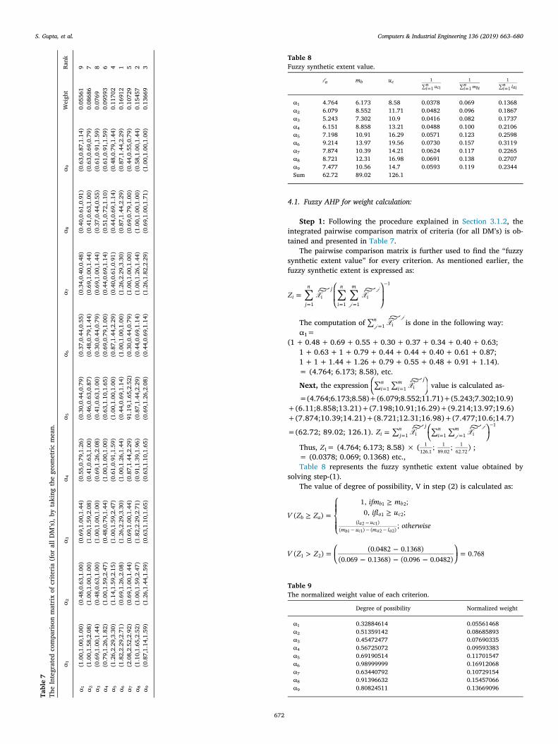
4.1. Fuzzy AHP for weight calculation:

Step 1: Following the procedure explained in Section 3.1.2, theintegrated pairwise comparison matrix of criteria (for all DM’s) is ob-tained and presented in Table 7.

The pairwise comparison matrix is further used to find the “fuzzysynthetic extent value” for every criterion. As mentioned earlier, thefuzzy synthetic extent is expressed as:

X Xj

j

== = =

Zij

n j

i

n m

1i

1 1i

1

The computation of Xj

j

=n

1 i is done in the following way:α1=

(1+0.48+0.69+0.55+0.30+0.37+0.34+0.40+0.63;1+0.63+1+0.79+ 0.44+ 0.44+ 0.40+ 0.61+ 0.87;1+1+1.44+ 1.26+ 0.79+ 0.55+ 0.48+ 0.91+ 1.14).= (4.764; 6.173; 8.58), etc.

Next, the expression X= =in

im j

1 1 i value is calculated as-

=(4.764;6.173;8.58)+(6.079;8.552;11.71)+(5.243;7.302;10.9)+(6.11;8.858;13.21)+(7.198;10.91;16.29)+(9.214;13.97;19.6)+(7.874;10.39;14.21)+(8.721;12.31;16.98)+(7.477;10.6;14.7)

=(62.72; 89.02; 126.1). X Xj

j

= = = =Zi jn j

in m

1 i 1 1 i

1

Thus, Z1= (4.764; 6.173; 8.58) × ( ; ; )1126.1

189.02

162.72 ;

= (0.0378; 0.069; 0.1368) etc.,Table 8 represents the fuzzy synthetic extent value obtained by

solving step-(1).The value of degree of possibility, V in step (2) is calculated as:

=V Z Z

ifm mifl u

otherwise( )

1, ;0, ;

;b a

b b

a cl u

m u m l

1 2

1 2( )

( ) ( )a c

b c a a2 1

1 1 2 2

> = =V Z Z( ) (0.0482 0.1368)(0.069 0.1368) (0.096 0.0482)

0.7681 2

Table7

TheIntegrated

comparisonmatrixof

criteria(for

allD

M’s),b

ytaking

thegeom

etricmean.

α 1α 2

α 3α 4

α 5α 6

α 7α 8

α 9Weight

Rank

α 1(1.00,1.00,1.00)

(0.48,0.63,1.00)

(0.69,1.00,1.44)

(0.55,0.79,1.26)

(0.30,0.44,0.79)

(0.37,0.44,0.55)

(0.34,0.40,0.48)

(0.40,0.61,0.91)

(0.63,0.87,1.14)

0.05561

9α 2

(1.00,1.58,2.08)

(1.00,1.00,1.00)

(1.00,1.59,2.08)

(0.41,0.63,1.00)

(0.46,0.63,0.87)

(0.48,0.79,1.44)

(0.69,1.00,1.44)

(0.41,0.63,1.00)

(0.63,0.69,0.79)

0.08686

7α 3

(0.69,1.00,1.44)

(0.48,0.63,1.00)

(1.00,1.00,1.00)

(0.69,1.26,2.08)

(0.41,0.63,1.00)

(0.30,0.44,0.79)

(0.69,1.00,1.44)

(0.37,0.44,0.55)

(0.61,0.91,1.59)

0.0769

8α 4

(0.79,1.26,1.82)

(1.00,1.59,2.47)

(0.48,0.79,1.44)

(1.00,1.00,1.00)

(0.63,1.10,1.65)

(0.69,0.79,1.00)

(0.44,0.69,1.14)

(0.51,0.72,1.10)

(0.61,0.91,1.59)

0.09593

6α 5

(1.26,2.29,3.30)

(1.14,1.59,2.15)

(1.00,1.59,2.47)

(0.61,0.91,1.59)

(1.00,1.00,1.00)

(0.87,1.44,2.29)

(0.40,0.61,0.91)

(0.44,0.69,1.14)

(0.48,0.79,1.44)

0.11702

4α 6

(1.82,2.29,2.71)

(0.69,1.26,2.08)

(1.26,2.29,3.30)

(1.00,1.26,1.44)

(0.44,0.69,1.14)

(1.00,1.00,1.00)

(1.26,2.29,3.30)

(0.87,1.44,2.29)

(0.87,1.44,2.29)

0.16912

1α 7

(2.08,2.52,2.92)

(0.69,1.00,1.44)

(0.69,1.00,1.44)

(0.87,1.44,2.29)

91.19,1.65,2.52)

(0.30,0.44,0.79)

(1.00,1.00,1.00)

(0.69,0.79,1.00)

(0.44,0.55,0.79)

0.10729

5α 8

(1.10,1.65,2.52)

(1.00,1.59,2.47)

(1.82,2.29,2.71)

(0.91,1.39,1.96)

(0.87,1.44,2.29)

(0.44,0.69,1.14)

(1.00,1.26,1.44)

(1.00,1.00,1.00)

(0.58,1.00,1.44)

0.15457

2α 9

(0.87,1.14,1.59)

(1.26,1.44,1.59)

(0.63,1.10,1.65)

(0.63,1.10,1.65)

(0.69,1.26,2.08)

(0.44,0.69,1.14)

(1.26,1.82,2.29)

(0.69,1.00,1.71)

(1.00,1.00,1.00)

0.13669

3

Table 8Fuzzy synthetic extent value.

la mb uc=i

n uci1

1 =in mbi

1

1 =in lai

1

1

α1 4.764 6.173 8.58 0.0378 0.069 0.1368α2 6.079 8.552 11.71 0.0482 0.096 0.1867α3 5.243 7.302 10.9 0.0416 0.082 0.1737α4 6.151 8.858 13.21 0.0488 0.100 0.2106α5 7.198 10.91 16.29 0.0571 0.123 0.2598α6 9.214 13.97 19.56 0.0730 0.157 0.3119α7 7.874 10.39 14.21 0.0624 0.117 0.2265α8 8.721 12.31 16.98 0.0691 0.138 0.2707α9 7.477 10.56 14.7 0.0593 0.119 0.2344Sum 62.72 89.02 126.1

Table 9The normalized weight value of each criterion.

Degree of possibility Normalized weight

α1 0.32884614 0.05561468α2 0.51359142 0.08685893α3 0.45472477 0.07690335α4 0.56725072 0.09593383α5 0.69190514 0.11701547α6 0.98999999 0.16912068α7 0.63440792 0.10729154α8 0.91396632 0.15457066α9 0.80824511 0.13669096


672

V(Z1 > Z3)= 0.883; V(Z1 > Z4)= 0.745; V Z( 1 > Z5)= 0.600 ;V(Z1 > Z6)= 0.421 ; V(Z1 > Z7)= 0.611 ;V Z( 1 > Z8)= 0.329;V(Z1 > Z9)= 0.611 etc.

The weights priority is calculated as;d''= (C1) min (0.768; 0.88; 0.75; 0.600; 0.42; 0.611; 0.329;

0.611)= 0.329;d''= (C2) min (1; 0.976; 0.830; 0.651; 0.857; 0.514;

0.850)= 0.514; etc.Similarly, the value of the remaining criteria are obtainedAfter computing the values in step (4), the weight and their nor-

malized value of each criterion is presented in Table 9.W ''= (0.329; 0.514; 0.455; 0.568; 0.691; 1.00; 0.634; 0.913; 0.808);W=

(0.0556;0.087;0.078;0.0959;0.117;0.1691;0.1072;0.1545;0.1366)

4.2. Fuzzy TOPSIS solution

Fuzzy-TOPSIS and fuzzy-WASPAS method hold a similar normal-ization process. The normalized fuzzy decision matrix (R normalized) isconstructed using Eqs. (6) and (7).

For GSS, the normalized value for r~11 and r~21 is calculated as:r~11= ( ), ,4.33

8.004.336.33

4.334.33 ; where la j = =lmin (4.33)

iaij , for cost criteria.

r~11= (0.54,0.68,1.00);r~21= ( ), ,5.00

9.677.009.67

8.669.67 ; where u *c j = umax

icij=(9.667), for benefit

criteria.r~21= (0.51,0.72,0.89);Similar, steps are followed to calculate values of other elements; the

complete normalized decision matrix is given in Table 10.After calculating the value of each element in the normalized ma-

trix, the subsequent step is to construct the weighted normalized matrix(Uij = r~ij·Wi using Eq. (9). Table 8 represents the weighted normal-ized matrix.

By considering Eqs. (10) and (11) distance measure of altenativesfrom Positive ( +di ) and negative ideal solution (di ) is calculated as;

= + + ++d 13

[((1 0.031) (1 0.038) (1 0.056) )]12 2 2

+ + +13

[((1 0.044) (1 0.062) (1 0.077) )]2 2 2

+ + =13

[((1 0.082) (1 0.112) (1 0.136) )] 8.2632 2 2

where +U j ={(1,1,1)}; U j ={(0,0,0)};Similarly, other values are calculated, and the obtained results are

shown in Table 12.Finally, w.r.t each green supplier, the value of the closeness coef-

ficient (Ci), is calculated using Eq. (12).

=+

=CiforGS 1 8.2638.263 0.744

0.08258

Based on obtained Ci value for each alternative as shown in

Table 12, it can be concluded by integrated fuzzy AHP and fuzzyTOPSIS results that, GSS1 with highest coefficient index value hold rank1, followed by GSS3, followed byGSS2 which holds rank 3 followed byGSS4 at last.

4.3. Fuzzy WASPAS solution

The fuzzy aggregated decision matrix for both fuzzy WASPAS andfuzzy TOPSIS methods are identical. The matrix is presented in Table 6.Subsequently, the weighted normalized decision matrix for both WSMand WPM is constructed. From Eq. (13) the obtained weighted nor-malized decision matrix for fuzzy-TOPSIS is the same as for WSM (X q)presented in Table 11.

For WPM, each element value in a “weighted normalized fuzzydecision matrix” (X p) is calculated as-

=X p( ) [(0.54) ; (0.68) ; (1.00) )];110.056 0.056 0.056

Similarly, the calculation steps for others elements will remainsame. Table 13 represents the weighted normalized matrix for WPM(X p).

The optimality function value is calculated for both WSM and WPMusing Eqs. (15) and (16).

For WSM, the value of optimality function for each alternative canbe calculated as;

Q1= (0.30+0.049+0.0345+ 0.0582+0.0975……0.0.0829;0.0380+0.629+0.0504+ 0.0788……………0.0.1122;0.0556+0.0778+0.0663+…………………….…0.1366)Q1= (0.555, 0.7285, 0.9312);Similarly, other values for WSM optimality function are calculated;For WPM, the optimality function value is calculated as;P1 = (0.96×0.94×0.94×0.953× 0.978× 0.924………0.93;0.98× 0.97× 0.96× 0.98× 0.99×………………0.97;1×0.99×0.98×1×1×……………………….….....1)P1 = (0.5359; 0.7089; 0.9236);De-fuzzify the obtained result by using equation (17) and (18).

Q = + + =13

(0.55 0.728 0.93) (0.7384);defuzzification1[ ]

P = + + =13

(0.535 0.70 0.923) (0.7228);defuzzification1[ ]

By using Eq. (19), the value of integrated utility function (IUF) infuzzy WASPAS method for an alternative (Ai ) is calculated as :

= 0.4912; K1= (0.4912*0.73)+(1–0.4912)*(0.7228)= 0.7305.Similarly, the value of ki can be calculated for other alternatives,

Table 14 shows obtained ki values. The maximumKI value defines thehighest rank of alternative., by Table 14 GS-1 Ki score is highest fol-lowed by GS-3, so the ranking order by hybrid fuzzy AHP and Fuzzy-WASPAS method is as follows GS-1 > GS-3 > GS-2 > GS-4.

4.4. Fuzzy MABAC solution:

By using Eqs. (22) and (23), values in the fuzzy normalized matrixfor cost criteria can be obtained as:

=r~ 8.00 9.6774.33 9.677

; 6.33 8.004.33 9.677

; 4.33 9.6674.33 9.677

;11

Thus, r~11 = (0.3125, 0.6250, 1.00).Table 15 represents the normalized matrix whose values are ob-

tained using similar steps explained previously.For weighted normalized matrix (Uij), value is calculated using Eq.

(24), and is presented in Table 16.By using Eq. (25), the border approximation area matrix of di-

mension (n×1) is formed. Table 17, presents the geometric meanvalue, and its calculation is as follows-

Table 10[TOPSIS] Normalized Matrix.

GS-1 GS-2 GS-3 GS-4

α1 (0.54,0.68,1.00) (0.44,0.52,0.68) (0.52,0.68,1.00) (0.46,0.56,0.76)α2 (0.51,0.72,0.89) (0.51,0.72,0.93) (0.65,0.86,1.00) (0.37,0.54,0.79)α3 (0.44,0.65,0.86) (0.24,0.44,0.65) (0.51,0.72,0.89) (0.65,0.86,1.00)α4 (0.60,0.82,1.00) (0.60,0.82,1.00) (0.60,0.82,0.96) (0.39,0.60,0.82)α5 (0.83,0.97,1.00) (0.63,0.83,0.97) (0.50,0.70,0.86) (0.50,0.70,0.86)α6 (0.62,0.85,1.00) (0.48,0.70,0.96) (0.62,0.85,1.00) (0.40,0.62,0.81)α7 (0.29,0.45,1.00) (0.20,0.26,0.35) (0.17,0.21,0.29) (0.22,0.29,0.45)α8 (0.44,0.52,0.68) (0.46,0.56,0.76) (0.54,0.68,1.00) (0.50,0.59,0.76)α9 (0.61,0.82,1.00) (0.39,0.60,0.82) (0.60,0.82,1.00) (0.46,0.67,0.85)


673

= × × ×g ([0.0730 0.0556 0.0695 0.0591] ;114

× × ×[0.090 0.069 0.090 0.076] ;14

× × ×[0.11 0.0903 0.112 0.097] ).14

Alternative distance from BAA matrix can be obtained by using Eq.(28) as

Q 1 = (0.0730–0.1021; 0.0904–0.0812; 0.111–0.063);Q 1 = (−0.0291; 0.0092; 0.0473);Similarly, other values are calculated and Table 18 represents the

distance of each alternative from BAA matrix.By Eq. (30), the overall value of criteria-function of alternatives

S ,i is obtained asSi = (−0.029+ (−0.053) + (−0.040) …………+ (−0.069);0.009+0.0006+………………………+0.021;0.047+0.053+……………………+0.109)Si = (−0.4982; 0.114046; 0.7107).Table 19 presents Si value for all the four alternatives. By defuzzi-

fying the Si value we rank the alternative based on defuzzified Siscore w.r.t each supplier. From the Table 19, it is observed that theranks of suppliers are similar from both integrated Fuzzy AHP withfuzzy TOPSIS and fuzzy AHP with WASPAS method. Green Supplier-1with the highest Si value of 0.1088 holds 1 position, followed bysupplier 3 and 2 with value (0.072245, −0.05921) and finally supplier4 with the lowest Si value (−0.0859) is ranked 4.

4.5. Consistency test

This test is performed in order to get ensure that the given expert’sinputs are consistent or not (Jain et al., 2018). Consistent inputs can bedefined in the matrix as the expert inputs that are neither illogical norrandom. In the fuzzy-AHP method, it is recommendable to test theconsistency ratio after performing the comparison (Kutlu &Ekmekçioğlu, 2012). For this, the “Graded mean integrated” method isused for the de-fuzzification process.

Let the given fuzzy-number be X = l m u( , ,a b c), it is converted intoa crisp number by the expression (31) (Kutlu & Ekmekçioğlu, 2012).

X X= = + +P l m u( 4. )6

a b c

(31)

By applying Eq. (31), each value gets deffuzified in the matrix, andconsistency-ratio (C-R) value is computed and compared with the ori-ginal CR value of 0.10, i.e. check the obtained value of CR is smallerthan the original value of ‘0.10′ or not. If the CR value is greater than0.10, then the expert will be requested to re-do the portion of thequestionnaire.

Values of consistency index is found out by Eq. (32):

=N

CI N( )1

max(32)

CR value is calculated by dividing the consistency index value byrandom consistency-index value. In the presented case study, the CIvalue is tested for each pairwise comparison matrix and the observedCR value for each pairwise matrix is less than 0.10. Thus, Table 20demonstrates that the obtained results are consistent in nature.

Table 11[TOPSIS] Weighted Normalized Matrix.

GS-1 GS-2 GS-3 GS-4

α1 (0.031,0.038,0.056) (0.024,0.028,0.038) (0.028,0.038,0.05) (0.025,0.031,0.042)α2 (0.044,0.062,0.077) (0.044,0.062,0.080) (0.056,0.074,0.086) (0.032,0.050,0.068)α3 (0.034,0.050,0.066) (0.018,0.034,0.050) (0.039,0.055,0.068) (0.050,0.066,0.076)α4 (0.058,0.078,0.095) (0.058,0.078,0.095) (0.058,0.078,0.092) (0.037,0.058,0.078)α5 (0.097,0.113,0.117) (0.074,0.097,0.131) (0.058,0.081,0.101) (0.058,0.081,0.101)α6 (0.106,0.144,0.169) (0.081,0.118,0.156) (0.106,0.144,0.169) (0.068,0.106,0.137)α7 (0.031,0.048,0.107) (0.022,0.028,0.041) (0.019,0.023,0.031) (0.024,0.031,0.048)α8 (0.069,0.080,0.105) (0.071,0.087,0.118) (0.083,0.105,0.154) (0.077,0.091,0.118)α9 (0.082,0.112,0.136) (0.053,0.082,0.112) (0.082,0.112,0.136) (0.063,0.092,0.117)

Table 12[TOPSIS] Final Analysis Result.

Alternative di+ di- Ci Rank

GS-1 8.263 0.744 0.08258 1GS-2 8.376 0.634 0.07036 3GS-3 8.286 0.716 0.07957 2GS-4 8.388 0.621 0.06884 4

Table 13[WASPAS] Weighted Normalized Matrix for WPM.

GSS1 GSS2 GSS3 GSS4

α1 (0.966,0.967,1.00) (0.956,0.964,0.979) (0.964,0.979,1.00) (0.959,0.968,0.985)α2 (0.944,0.972,0.99) (0.944,0.972,0.993) (0.963,0.987,1.00) (0.919,0.954,0.980)α3 (0.941,0.968,0.98) (0.896,0.940,0.968) (0.95,0.975,0.991) (0.968,0.988,1.000)α4 (0.953,0.981,1.00) (0.953,0.981,1.000) (0.95,0.981,0.996) (0.914,0.953,0.982)α5 (0.978,0.996,1.00) (0.947,0.978,0.996) (0.92,0.959,0.983) (0.921,0.959,0.983)α6 (0.924,0.973,1.00) (0.883,0.942,0.987) (0.924,0.976,1.00) (0.859,0.924,0.965)α7 (0.877,0.918,1.00) (0.845,0.866,0.902) (0.83,0.849,0.877) (0.853,0.877,0.918)α8 (0.883,0.903,0.93) (0.888,0.915,0.959) (0.909,0.944,1.00) (0.898,0.921,0.959)α9 (0.934,0.973,1.00) (0.880,0.934,0.973) (0.934,0.973,1.00) (0.900,0.948,0.979)

Table 14[WASPAS] Final Result.

Alternatives Qi Pi Ki Rank

GS-1 0.738369 0.72281 0.730450 1GS-2 0.625412 0.59982 0.612391 3GS-3 0.715323 0.67765 0.696153 2GS-4 0.613373 0.59874 0.605926 4


674

4.6. Sensitivity analysis

The purpose of performing sensitivity analysis (SA) in the decision-making problems is to test the consequences of the weights of criteria.Based on different scenarios obtained in analysis, it can result inchanged alternative precedence. By varying the importance of criteria,if the obtained order of ranking changes, it can be referred that theobtained results are sensitive else robust in nature. SA may also offerinsight to the decision-makers at the conditions where uncertaintiesexist in the definition of the importance of different factors. l. Inter-changing of the weights of one criterion with other is done in order toknow that does the exchange of weight results in a change in the pre-cedence of alternatives (Senthil, Murugananthan, & Ramesh, 2018). In

order to do so, 36 experiments were performed and the closenesscoefficient (CCj) value was obtained. Further, the radar graph is alsoplotted (Fig. 6b) where α.x-y denotes the weights, interchanged be-tween criteria x and criteria y whereas else criteria weights remainunchanged.

In this case study, it can be concluded from the radar plot (6-b) andline plot (6-a) that the GS-1 alternative score has the highest score in all36 experiments. Followed by GS-3, whereas GS-2 and GS-4 are

Table 15[MABAC] Normalized Matrix.

GS-1 GS-2 GS-3 GS-4

α1 (0.312,0.625,1.00) (0.00,0.25,0.625) (0.250,0.625,1.00) (0.068,0.375,0.75)α2 (0.2220.556,0.833) (0.22,0.556,0.889) (0.444,0.778,1.00) (0.00,0.333,0.667)α3 (0.27,0.545,0.818) (0.00,0.273,0.546) (0.364,0.636,0.86) (0.545,0.818,1.00)α4 (0.352,0.705,1.00) (0.352,0.705,1.00) (0.358,0.706,0.94) (0.00,0.352,0.706)α5 (0.667,0.932,1.00) (0.267,0.667,0.93) (0.000,0.40,0.733) (0.000,0.40,0.733)α6 (0.375,0.751,1.00) (0.125,0.50,0.875) (0.375,0.751,1.00) (0.00,0.375,0.685)α7 (0.478,0.739,1.00) (0.173,0.3917,0.65) (0.000,0.21,0.477) (0.261,0.478,0.79)α8 (0.000,0.25,0.625) (0.068,0.375,0.75) (0.325,0.625,1.00) (0.185,0.435,0.75)α9 (0.352,0.705,1.00) (0.00,0.352,0.706) (0.352,0.705,1.00) (0.117,0.478,0.761)

Table 16[MABAC] Weighted Normalized Matrix.

GS-1 GS-2 GS-3 GS-4

α1 (0.072, 0.090, 0.111) (0.055, 0.069, 0.090) (0.069, 0.090, 0.112) (0.059, 0.076, 0.097)α2 (0.191, 0.135, 0.159) (0.106, 0.135, 0.166) (0.125, 0.154, 0.173) (0.086, 0.115, 0.147)α3 (0.097, 0.115, 0.139) (0.076, 0.093, 0.115) (0.104, 0.125, 0.143) (0.111, 0.132, 0.158)α4 (0.129, 0.169, 0.198) (0.129, 0.169, 0.191) (0.129, 0.163, 0.182) (0.095, 0.129, 0.163)α5 (0.195, 0.226, 0.234) (0.148, 0.195, 0.226) (0.117, 0.168, 0.228) (0.170 ,0.168, 0.202)α6 (0.235, 0.295, 0.338) (0.190, 0.253, 0.317) (0.235, 0.295, 0.338) (0.169, 0.235, 0.285)α7 (0.158, 0.186, 0.214) (0.125, 0.149, 0.177) (0.107, 0.130, 0.158) (0.135, 0.158, 0.186)α8 (0.154, 0.193, 0.251) (0.164, 0.212, 0.270) (0.202, 0.251, 0.301) (0.183, 0.222, 0.270)α9 (0.184, 0.235, 0.273) (0.136, 0.184, 0.231) (0.184, 0.231, 0.273) (0.152, 0.206, 0.242)

Table 17[MABAC] Border Approximation Area Matrix.

Criteria BAA

α1 (0.063, 0.081, 0.102)α2 (0.105, 0.134, 0.153)α3 (0.098, 0.119, 0.138)α4 (0.120, 0.154, 0.182)α5 (0.141, 0.185, 0.216)α6 (0.204, 0.268, 0.318)α7 (0.130, 0.154, 0.183)α8 (0.175, 0.218, 0.274)α9 (0.163, 0.211, 0.254)

Table 18[MABAC] Distance of Alternative from BAA Matrix.

GS-1 GS-2 GS-3 GS-4

α1 (−0.029, 0.009, 0.047) (−0.046,− 0.011, 0.026) (‑0.032, 0.009, 0.047) (−0.043,−0.004, 0.031)α2 (−0.053, 0.006, 0.053) (−0.053, 0.006, 0.0581) (−0.034, 0.019, 0.068) (−0.073,−0.080, 0.039)α3 (−0.040,−0.007, 0.041) (−0.061,−0.021, 0.020) (−0.033, 0.006, 0.044) (−0.019, 0.020, 0.055)α4 (−0.053, 0.009, 0.071) (−0.053, 0.009, 0.0712) (−0.053, 0.009, 0.065) (−0.087,−0.024, 0.043)α5 (−0.021, 0.040, 0.092) (−0.067, 0.009, 0.0850) (−0.09,−0.021, 0.064) (−0.099,−0.021, 0.061)α6 (−0.086, 0.027, 0.133) (−0.128,−0.014, 0.112) (−0.086, 0.020, 0.130) (−0.149,−0.031, 0.081)α7 (−0.024, 0.031, 0.084) (−0.057,−0.005, 0.046) (−0.075,−0.024, 0.028) (−0.047, 0.003, 0.056)α8 (−0.119,−0.02, 0.075) (−0.110,−0.006, 0.095) (−0.071, 0.032, 0.133) (−0.090, 0.003, 0.095)α9 (−0.069, 0.021, 0.109) (−0.117,−0.027, 0.069) (−0.069, 0.021, 0.109) (−0.101,−0.011, 0.077)

Table 19[MABAC] Final Result.

Alternative Si Defuzzification of Si Rank

GS-1 −0.49827 0.114046 0.710756 0.10884552 1GS-2 −0.69687 −0.06744 0.586667 −0.0592136 3GS-3 −0.55645 0.079933 0.693884 0.07245597 2GS-4 −0.71222 −0.08897 0.543327 −0.0859526 4

Table 20Consistency computation in AHP.

Items Values

Maximum Eigen value (λmax) 9.3059Consistency Index (CI) 0.0382Random Index (RI) at n= 9 0.0880Consistency ratio (CR) 0.4348


675

relatively quite close with each other even though GSS 2 score isslightly higher than GS-4 score Since by varying the importance of thecriterion, the alternative precedence remains unchanged, therefore itcan be concluded that obtained results are robust in nature.

4.7. Normalization

Normalization is a process used to eliminate the criteria units so thatthey become dimension less and encompasses values between 0 and 1.Sałabun (2013) has applied several normalization processes for theTOPSIS method. Two types of normalization procedures that are com-monly defined are linear normalization and vector normalization. Thekey difference between these two normalization procedures is that theresults scaled by the vector normalization process are dependent on theevaluation criteria whereas, in the case of linear normalization, it isindependent of the original units of the data (Banaeian et al., 2015). Inthis case study, the applied MCDM methods follows the linear nor-malization process.

From table 21, it can be observed that by performing a vector

Fig. 6. (a) Line plot for sensitivity analysis. (b) Radar plot for sensitivity analysis.

Table 21[TOPSIS] Obtained green supplier ranking results under different normalizationmethods.

Green linear normalization Vector normalizationSupplier Ci Ci

GS-1 0.08258(1) 0.08064(1)GS-2 0.07036(3) 0.06953(3)GS-3 0.07956(2) 0.07664(2)GS-4 0.06884(4) 0.06142(4)


676

normalization process in fuzzy-TOPSIS, the obtained ranking resultsremain unchanged. Therefore, the obtained ranking results will be in-dependent of the adopted normalization function.

5. Managerial implications

In the proposed case study, an effective method for GSS with

prominence on G-SCM issues has been established. Managers of alliedbusinesses can utilize the proposed framework to evaluate their sup-pliers. Thus, the obtained results can be utilized as a guideline for thesupply chain of the organization such that it does not allow to enter aninsignificant supplier in the supply chain. This will help in noteworthyresource and cost-saving and lessening of the environmental impacts.

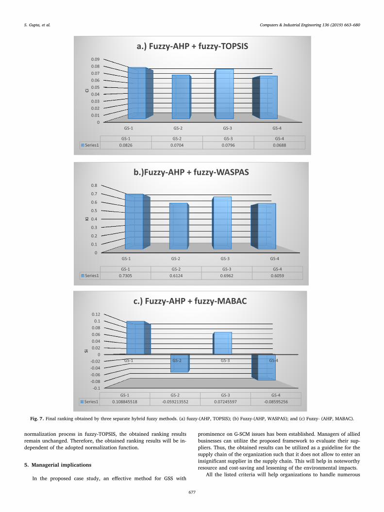
All the listed criteria will help organizations to handle numerous

Fig. 7. Final ranking obtained by three separate hybrid fuzzy methods. (a) fuzzy-(AHP, TOPSIS); (b) Fuzzy-(AHP, WASPAS); and (c) Fuzzy- (AHP, MABAC).


677

challenges and to improve their efforts to develop eco-friendly pro-ducts. Additionally, the significant advantage of this proposed work isthe development of GSS evaluation criteria by means of industry ex-pert’s response and literature. The applied sensitivity analysis will allowmanagers to test the observation stability.

6. Results and conclusion

The fusion of environmental criteria in the process of green supplierselection processes is attaining more importance day by day. Theavailability and development of new supplier selection models andanalytical tools can aid DM’s and managers by addressing numerouschallenges faced in procurement processes by supply chain manage-ment professionals.

The presented research work introduces a fuzzy-based rankingmodel for green supplier selection in the Indian automotive industry.The trustworthiness of the proposed integrated framework is presentedby considering a case study of the Indian automotive industry. Differentevaluation criteria were shortlisted from literature and consulting in-dustry experts. Finally, ‘nine’ criteria were shortlisted considering bothconventional and environment criteria by aggregating the expert's in-puts, aggregated pair-wise comparison matrix was constructed, fromwhich weights are obtained by applying Chang’s extended form of fuzzyAHP method. Evaluation criteria that have obtained maximum weightpriority in the analysis are ‘environmental management system’ ‘pol-lution control’, ’quality’ and ‘green image’, which later have been em-ployed as an input for the other three methods in order to select thepotential alternative Further set of suppliers were analyzed by in-tegrating three popular decisions. making method, fuzzy-TOPSIS, fuzzy-MABAC, and fuzzy-WASPAS with fuzzy-AHP. Results obtained supportsthe similar green supplier ranking as presented in Fig. 7(a), (b) and (c).

The consistency test was also performed for the purpose to check theconsistency of the expert’s inputs. Additionally, a sensitivity analysiswas performed to check the robustness of the applied system which ispresented in Fig. 6(a), (b). Results depict that the first alternative (GS-1)acquired the highest score followed by a third (GS-3). However, there isa small hazy line between GS-2 and 3, but the final score of GS-2 isgreater than GS-3. Hence, the ranking of GS in descending order isobtained as GS-1 > GS-3 > GS-2 > GS-4. Table 22, representsoverall results obtained from different hybrid MCDM techniques.

In the presented case study, the applied methods follow the samenormalization process. By differing, their normalization in fuzzy AHPand fuzzy-TOPSIS does not alter the obtained rank. This study delivers asingle platform or framework for GSS under fuzzy environment andprovides the stage for further exploration in this most significant anddeveloping knowledge area. Generally, DM's used to express their as-sessments in the linguistic term rather than pure numbers. So, the de-gree of subjectivity is reserved in the presented integrated models. Butin the applied models’ authors introduced the way to mitigate thesubjectivity in the problems of decision making.

For further research, this methodology can also accommodate thedynamic and uncertain environment by including novel factors af-fecting the change. This research could be applied to specific supplychain cases of industries such as electronics, textiles, food and oil &gasin order to test the general validity of the results. Future research could

also use different decision-making tools like VIKOR, PROMETHEE, andGRA. A limitation in the proposed model is that subsystems associatedwith the criterions are not considered to minimize complexity. Whileseveral efforts have been made for the green supplier selection, bearingin mind environmental subject remains a challenge. Additionally, howto allocate orders to the potential green suppliers in the model will be amatter for future research.

Appendix A. Supplementary material

Supplementary data to this article can be found online at https://doi.org/10.1016/j.cie.2019.07.038.

References

Aksoy, A., Sucky, E., & Öztürk, N. (2014). Dynamic strategic supplier selection systemwith fuzzy logic. Procedia-Social and Behavioral Sciences, 109, 1059–1063.

Amid, A., Ghodsypour, S. H., & O'Brien, C. (2006). A fuzzy multiobjective linear model forsupplier selection in a supply chain. International Journal of production economics,104(2), 394–407.

Amindoust, A., Ahmed, S., Saghafinia, A., & Bahreininejad, A. (2012). Sustainable sup-plier selection: A ranking model based on fuzzy inference system. Applied SoftComputing, 12(6), 1668–1677.

Anojkumar, L., Ilangkumaran, M., & Sasirekha, V. (2014). Comparative analysis of MCDMmethods for pipe material selection in sugar industry. Expert Systems with Applications,41(6), 2964–2980.

Awasthi, A., & Omrani, H. (2019). A goal-oriented approach based on fuzzy axiomaticdesign for sustainable mobility project selection. International Journal of SystemsScience: Operations & Logistics, 6(1), 86–98.

Awasthi, A., Chauhan, S. S., & Goyal, S. K. (2010). A fuzzy multicriteria approach forevaluating environmental performance of suppliers. International Journal ofProduction Economics, 126(2), 370–378.

Azadi, M., Jafarian, M., Saen, R. F., & Mirhedayatian, S. M. (2015). A new fuzzy DEAmodel for evaluation of efficiency and effectiveness of suppliers in sustainable supplychain management context. Computers & Operations Research, 54, 274–285.

Bai, C., & Sarkis, J. (2010). Integrating sustainability into supplier selection with greysystem and rough set methodologies. International Journal of Production Economics,124(1), 252–264.

Bali, O., Kose, E., & Gumus, S. (2013). Green supplier selection based on IFS and GRA.Grey Systems: Theory and Application, 3(2), 158–176.

Banaeian, N., Mobli, H., Nielsen, I. E., & Omid, M. (2015). Criteria definition and ap-proaches in green supplier selection–a case study for raw material and packaging offood industry. Production & Manufacturing Research, 3(1), 149–168.

Bellman, R. E., & Zadeh, L. A. (1970). Decision-making in a fuzzy environment.Management Science, 17(4), B-141.

Bevilacqua, M., Ciarapica, F. E., & Giacchetta, G. (2006). A fuzzy-QFD approach tosupplier selection. Journal of Purchasing and Supply Management, 12(1), 14–27.

Bozanic, D., Tešić, D., & Milićević, J. (2018). A hybrid fuzzy AHP-MABAC model:Application in the Serbian Army-The selection of the location for deep wading as atechnique of crossing the river by tanks. Decision Making: Applications in Managementand Engineering, 1(1), 143–164.

Büyüközkan, G., & Çifçi, G. (2012). A novel hybrid MCDM approach based on fuzzyDEMATEL, fuzzy ANP and fuzzy TOPSIS to evaluate green suppliers. Expert Systemswith Applications, 39(3), 3000–3011.

Carlsson, C., & Fullér, R. (1996). Fuzzy multiple criteria decision making: Recent devel-opments. Fuzzy sets and systems, 78(2), 139–153.

Chang, D. Y. (1996). Applications of the extent analysis method on fuzzy AHP. EuropeanJournal of Operational Research, 95(3), 649–655.

Chen, C. C., Tseng, M. L., Lin, Y. H., & Lin, Z. S. (2010). Implementation of green supplychain management in uncertainty. 2010 IEEE International Conference on IndustrialEngineering and Engineering Management (pp. 260–264). IEEE.

Chen, C. T. (2000). Extensions of the TOPSIS for group decision-making under fuzzyenvironment. Fuzzy Sets and Systems, 114(1), 1–9.

Chen, J. J. G., & He, Z. (1997). Using analytic hierarchy process and fuzzy set theory torate and rank the disability. Fuzzy Sets and Systems, 88(1), 1–22.

Chen, L. Y., & Wang, T. C. (2009). Optimizing partners’ choice in IS/IT outsourcingprojects: The strategic decision of fuzzy VIKOR. International Journal of ProductionEconomics, 120(1), 233–242.

Chen, Y. J., Wu, Y. J., & Wu, T. (2015). Moderating effect of environmental supply chaincollaboration: Evidence from Taiwan. International Journal of Physical Distribution &Logistics Management, 45(9/10), 959–978.

Choi, T. M. (2013). Optimal apparel supplier selection with forecast updates under carbonemission taxation scheme. Computers & Operations Research, 40(11), 2646–2655.

De Boer, L., Labro, E., & Morlacchi, P. (2001). A review of methods supporting supplierselection. European Journal of Purchasing & Supply Management, 7(2), 75–89.

Dos Santos, B. M., Godoy, L. P., & Campos, L. M. (2019). Performance evaluation of greensuppliers using entropy-TOPSIS-F. Journal of Cleaner Production, 207, 498–509.

Dotoli, M., Epicoco, N., Falagario, M., & Sciancalepore, F. (2015). A cross-efficiency fuzzydata envelopment analysis technique for performance evaluation of decision makingunits under uncertainty. Computers & Industrial Engineering, 79, 103–114.

Dubey, R., Gunasekaran, A., Sushil, & Singh, T. (2015). Building theory of sustainable

Table 22Numerical results of three hybrid MCDM technique.

RANK RANK RANKF-[AHP,TOPSIS] F-[AHP,WASPAS] F-[AHP,MABAC]Ci Ki Si

GS-1 0.08258(1) 0.7304(1) 0.1088(1)GS-2 0.07036(3) 0.6123(3) −0.0591(3)GS-3 0.07956(2) 0.6961(2) 0.0724(2)GS-4 0.06884(4) 0.6059(4) −0.0859(4)


678



http://refhub.elsevier.com/S0360-8352(19)30429-2/h0005






























































http://refhub.elsevier.com/S0360-8352(19)30429-2/optOoVXzUnZip




manufacturing using total interpretive structural modelling. International Journal ofSystems Science: Operations & Logistics, 2(4), 231–247.

Easton, A. (1973). One-of-a-kind decisions involving weighted multiple objectives anddisparate alternatives. Multiple Criteria Decision Making, 657–667.

Fahimnia, B., Sarkis, J., Choudhary, A., & Eshragh, A. (2015). Tactical supply chainplanning under a carbon tax policy scheme: A case study. International Journal ofProduction Economics, 164, 206–215.

Farzad, T. & Aidy, A. (2008). A review of supplier selection methods in manufacturingindustries.

Fu, Y. K. (2019). An integrated approach to catering supplier selection using AHP-ARAS-MCGP methodology. Journal of Air Transport Management, 75, 164–169.

Galankashi, M. R., Helmi, S. A., & Hashemzahi, P. (2016). Supplier selection in auto-mobile industry: A mixed balanced scorecard–fuzzy AHP approach. AlexandriaEngineering Journal, 55(1), 93–100.

Gharaei, A., Hoseini Shekarabi, S. A., & Karimi, M. (2019a). Modelling And optimal lot-sizing of the replenishments in constrained, multi-product and bi-objective EPQmodels with defective products: Generalised Cross Decomposition. InternationalJournal of Systems Science: Operations & Logistics, 1–13.

Gharaei, A., Karimi, M., & Hoseini Shekarabi, S. A. (2019b). Joint Economic Lot-sizing inMulti-product Multi-level Integrated Supply Chains: Generalized BendersDecomposition. International Journal of Systems Science: Operations & Logistics, 1–17.

Gharaei, A., Karimi, M., & Shekarabi, S. A. H. (2019c). An integrated multi-product,multi-buyer supply chain under penalty, green, and quality control polices and avendor managed inventory with consignment stock agreement: The outer approx-imation with equality relaxation and augmented penalty algorithm. AppliedMathematical Modelling, 69, 223–254.

Govindan, K., Khodaverdi, R., & Jafarian, A. (2013). A fuzzy multi criteria approach formeasuring sustainability performance of a supplier based on triple bottom line ap-proach. Journal of Cleaner Production, 47, 345–354.

Govindan, K., Rajendran, S., Sarkis, J., & Murugesan, P. (2015). Multi criteria decisionmaking approaches for green supplier evaluation and selection: A literature review.Journal of Cleaner Production, 98, 66–83.

Guo, X., Yuan, Z., & Tian, B. (2009). Supplier selection based on hierarchical potentialsupport vector machine. Expert Systems with Applications, 36(3), 6978–6985.

Gupta, H., & Barua, M. K. (2017). Supplier selection among SMEs on the basis of theirgreen innovation ability using BWM and fuzzy TOPSIS. Journal of Cleaner Production,152, 242–258.

Handfield, R., Walton, S. V., Sroufe, R., & Melnyk, S. A. (2002). Applying environmentalcriteria to supplier assessment: A study in the application of the analytical hierarchyprocess. European Journal of Operational Research, 141(1), 70–87.

Hao, Y., Helo, P., & Shamsuzzoha, A. (2018). Virtual factory system design and im-plementation: Integrated sustainable manufacturing. International Journal of SystemsScience: Operations & Logistics, 5(2), 116–132.

Hashemi, S. H., Karimi, A., & Tavana, M. (2015). An integrated green supplier selectionapproach with analytic network process and improved Grey relational analysis.International Journal of Production Economics, 159, 178–191.

Hoseini Shekarabi, S. A., Gharaei, A., & Karimi, M. (2018). Modelling and optimal lot-sizing of integrated multi-level multi-wholesaler supply chains under the shortageand limited warehouse space: Generalised outer approximation. International Journalof Systems Science: Operations & Logistics, 1–21.

Hsu, B. M., Chiang, C. Y., & Shu, M. H. (2010). Supplier selection using fuzzy quality dataand their applications to touch screen. Expert Systems with Applications, 37(9),6192–6200.

Humphreys, P. K., Wong, Y. K., & Chan, F. T. S. (2003). Integrating environmental criteriainto the supplier selection process. Journal of Materials Processing Technology,138(1–3), 349–356.

Hussey, D. M., & Eagan, P. D. (2007). Using structural equation modeling to test en-vironmental performance in small and medium-sized manufacturers: Can SEM helpSMEs? Journal of Cleaner Production, 15(4), 303–312.

Hwang, C. L., & Yoon, K. S. (1981). Multiple attribute decision-making. Methods and appli-cations. Springer Verlag58–191.

Jain, V., Sangaiah, A. K., Sakhuja, S., Thoduka, N., & Aggarwal, R. (2018). Supplier se-lection using fuzzy AHP and TOPSIS: A case study in the Indian automotive industry.Neural Computing and Applications, 29(7), 555–564.

KarimiAzari, A., Mousavi, N., Mousavi, S. F., & Hosseini, S. (2011). Risk assessment modelselection in construction industry. Expert Systems with Applications, 38(8), 9105–9111.

Kazemi, N., Abdul-Rashid, S. H., Ghazilla, R. A. R., Shekarian, E., & Zanoni, S. (2018).Economic order quantity models for items with imperfect quality and emissionconsiderations. International Journal of Systems Science: Operations & Logistics, 5(2),99–115.

Kirytopoulos, K., Leopoulos, V., & Voulgaridou, D. (2008). Supplier selection in phar-maceutical industry: An analytic network process approach. Benchmarking: AnInternational Journal, 15(4), 494–516.

Kull, T. J., & Talluri, S. (2008). A supply risk reduction model using integrated multi-criteria decision making. IEEE Transactions on Engineering Management, 55(3),409–419.

Kuo, R. J., Hong, S. Y., & Huang, Y. C. (2010). Integration of particle swarm optimization-based fuzzy neural network and artificial neural network for supplier selection.Applied Mathematical Modelling, 34(12), 3976–3990.

Kusi-Sarpong, S., Bai, C., Sarkis, J., & Wang, X. (2015). Green supply chain practicesevaluation in the mining industry using a joint rough sets and fuzzy TOPSIS meth-odology. Resources Policy, 46, 86–100.

Kutlu, A. C., & Ekmekçioğlu, M. (2012). Fuzzy failure modes and effects analysis by usingfuzzy TOPSIS-based fuzzy AHP. Expert Systems with Applications, 39(1), 61–67.

Lashgari, S., Antuchevičienė, J., Delavari, A., & Kheirkhah, O. (2014). Using QSPM andWASPAS methods for determining outsourcing strategies. Journal of Business

Economics and Management, 15(4), 729–743.Lee, A. H., Kang, H. Y., Hsu, C. F., & Hung, H. C. (2009). A green supplier selection model

for high-tech industry. Expert Systems with Applications, 36(4), 7917–7927.Lee, C. C., & Ou-Yang, C. (2009). A neural networks approach for forecasting the sup-

plier’s bid prices in supplier selection negotiation process. Expert Systems withApplications, 36(2), 2961–2970.

Levary, R. R. (2008). Using the analytic hierarchy process to rank foreign suppliers basedon supply risks. Computers & Industrial Engineering, 55(2), 535–542.

Li, G. D., Yamaguchi, D., & Nagai, M. (2007). A grey-based decision-making approach tothe supplier selection problem. Mathematical and Computer Modelling, 46(3–4),573–581.

Liao, C. N., & Kao, H. P. (2011). An integrated fuzzy TOPSIS and MCGP approach tosupplier selection in supply chain management. Expert Systems with Applications,38(9), 10803–10811.

Lin, C. T., Chen, C. B., & Ting, Y. C. (2011). An ERP model for supplier selection inelectronics industry. Expert Systems with Applications, 38(3), 1760–1765.

Lin, Y. T., Lin, C. L., Yu, H. C., & Tzeng, G. H. (2010). A novel hybrid MCDM approach foroutsourcing vendor selection: A case study for a semiconductor company in Taiwan.Expert Systems with Applications, 37(7), 4796–4804.

Liu, T., Deng, Y., & Chan, F. (2018). Evidential supplier selection based on DEMATEL andgame theory. International Journal of Fuzzy Systems, 20(4), 1321–1333.

MacCrimmon, K. R. (1968). Decisionmaking among multiple-attribute alternatives: asurvey and consolidated approach (No. RM-4823-ARPA). RAND CORP SANTAMONICA CA.

Mavi, R. K., Goh, M., & Mavi, N. K. (2016). Supplier selection with Shannon entropy andfuzzy TOPSIS in the context of supply chain risk management. Procedia-Social andBehavioral Sciences, 235, 216–225.

Nallusamy, S., Sri Lakshmana Kumar, D., Balakannan, K., & Chakraborty, P. S. (2016).MCDM tools application for selection of suppliers in manufacturing industries usingAHP, Fuzzy Logic and ANN. In International Journal of Engineering Research inAfrica (Vol. 19, pp. 130–137). Trans Tech Publications.

Noci, G. (1997). Designing ‘green’vendor rating systems for the assessment of a supplier'senvironmental performance. European Journal of Purchasing & Supply Management,3(2), 103–114.

Önüt, S., Kara, S. S., & Işik, E. (2009). Long term supplier selection using a combinedfuzzy MCDM approach: A case study for a telecommunication company. ExpertSystems with Applications, 36(2), 3887–3895.

Pamučar, D., & Ćirović, G. (2015). The selection of transport and handling resources inlogistics centers using Multi-Attributive Border Approximation area Comparison(MABAC). Expert Systems with Applications, 42(6), 3016–3028.

Paul, S. K. (2015). Supplier selection for managing supply risks in supply chain: A fuzzyapproach. The International Journal of Advanced Manufacturing Technology, 79(1–4),657–664.

Peng, X., & Yang, Y. (2016). Pythagorean fuzzy Choquet integral based MABAC methodfor multiple attribute group decision making. International Journal of IntelligentSystems, 31(10), 989–1020.

Perçin, S. (2019). An integrated fuzzy SWARA and fuzzy AD approach for outsourcingprovider selection. Journal of Manufacturing Technology Management, 30(2), 531–552.

Rabbani, M., Foroozesh, N., Mousavi, S. M., & Farrokhi-Asl, H. (2019). Sustainable sup-plier selection by a new decision model based on interval-valued fuzzy sets andpossibilistic statistical reference point systems under uncertainty. InternationalJournal of Systems Science: Operations & Logistics, 6(2), 162–178.

Rabbani, M., Hosseini-Mokhallesun, S. A. A., Ordibazar, A. H., & Farrokhi-Asl, H. (2018).A hybrid robust possibilistic approach for a sustainable supply chain location-allo-cation network design. International Journal of Systems Science: Operations & Logistics,1–16.

Roy, J., Chatterjee, K., Bandyopadhyay, A., & Kar, S. (2018). Evaluation and selection ofmedical tourism sites: A rough analytic hierarchy process based multi-attributiveborder approximation area comparison approach. Expert Systems, 35(1), e12232.

Roy, J., Ranjan, A., & Kar, S. (2016). An extended MABAC for multi-attribute decisionmaking using trapezoidal interval type-2 fuzzy numbers. arXiv preprintarXiv:1607.01254.

Saen, R. F. (2010). Developing a new data envelopment analysis methodology for supplierselection in the presence of both undesirable outputs and imprecise data. TheInternational Journal of Advanced Manufacturing Technology, 51(9–12), 1243–1250.

Sałabun, Wojciech. (2003). X. 1. Normalization of attribute values in TOPSIS method.Sanayei, A., Mousavi, S. F., & Yazdankhah, A. (2010). Group decision making process for

supplier selection with VIKOR under fuzzy environment. Expert Systems withApplications, 37(1), 24–30.

Sarkis, J. (2012). A boundaries and flows perspective of green supply chain management.Supply Chain Management: An International Journal, 17(2), 202–216.

Sayyadi, R., & Awasthi, A. (2018a). A simulation-based optimisation approach for iden-tifying key determinants for sustainable transportation planning. International Journalof Systems Science: Operations & Logistics, 5(2), 161–174.

Sayyadi, R., & Awasthi, A. (2018b). An integrated approach based on system dynamicsand ANP for evaluating sustainable transportation policies. International Journal ofSystems Science: Operations & Logistics, 1–10.

Seiford, L. M. (1996). Data envelopment analysis: The evolution of the state of the art(1978–1995). Journal of Productivity Analysis, 7(2–3), 99–137.

Senthil, S., Murugananthan, K., & Ramesh, A. (2018). Analysis and prioritisation of risksin a reverse logistics network using hybrid multi-criteria decision making methods.Journal of Cleaner Production, 179, 716–730.

Sevkli, M. (2010). An application of the fuzzy ELECTRE method for supplier selection.International Journal of Production Research, 48(12), 3393–3405.

Sharma, V. K., Chandna, P., & Bhardwaj, A. (2017). Green supply chain managementrelated performance indicators in agro industry: A review. Journal of Cleaner


679








http://refhub.elsevier.com/S0360-8352(19)30429-2/optfhorWGgjQ4

http://refhub.elsevier.com/S0360-8352(19)30429-2/optfhorWGgjQ4
























http://refhub.elsevier.com/S0360-8352(19)30429-2/optWKmQNaUm0v

























http://refhub.elsevier.com/S0360-8352(19)30429-2/opt3nyjv80hE5

http://refhub.elsevier.com/S0360-8352(19)30429-2/opt3nyjv80hE5














































































http://refhub.elsevier.com/S0360-8352(19)30429-2/optzGp0rwXNdP


























Production, 141, 1194–1208.Shen, L., Olfat, L., Govindan, K., Khodaverdi, R., & Diabat, A. (2013). A fuzzy multi

criteria approach for evaluating green supplier's performance in green supply chainwith linguistic preferences. Resources, Conservation and Recycling, 74, 170–179.

Tong, R. M., & Bonissone, P. P. (1980). A linguistic approach to decisionmaking withfuzzy sets. IEEE Transactions on Systems, Man, and Cybernetics, 10(11), 716–723.

Trapp, A. C., & Sarkis, J. (2016). Identifying Robust portfolios of suppliers: A sustain-ability selection and development perspective. Journal of Cleaner Production, 112,2088–2100.

Tsai, S. B., Wei, Y. M., Chen, K. Y., Xu, L., Du, P., & Lee, H. C. (2016). Evaluating greensuppliers from a green environmental perspective. Environment and Planning B:Planning and Design, 43(5), 941–959.

Tseng, M. L., Wang, R., Chiu, A. S., Geng, Y., & Lin, Y. H. (2013). Improving performanceof green innovation practices under uncertainty. Journal of cleaner production, 40,71–82.

Turskis, Z., Zavadskas, E. K., Antucheviciene, J., & Kosareva, N. (2015). A hybrid modelbased on fuzzy AHP and fuzzy WASPAS for construction site selection. InternationalJournal of Computers Communications & Control, 10(6), 113–128.

Wang Chen, H. M., Chou, S. Y., Luu, Q. D., & Yu, T. H. K. (2016). A fuzzy MCDM approachfor green supplier selection from the economic and environmental aspects.Mathematical Problems in Engineering.

Wang, T. C., & Chang, T. H. (2007). Application of TOPSIS in evaluating initial trainingaircraft under a fuzzy environment. Expert Systems with Applications, 33(4), 870–880.

Wang, X. (2015). A comprehensive decision making model for the evaluation of greenoperations initiatives. Technological Forecasting and Social Change, 95, 191–207.

Wang, Y. M., & Elhag, T. M. (2006). Fuzzy TOPSIS method based on alpha level sets withan application to bridge risk assessment. Expert Systems with Applications, 31(2),309–319.

Weber, C. A., Current, J. R., & Benton, W. C. (1991). Vendor selection criteria and

methods. European Journal of Operational Research, 50(1), 2–18.Wu, D. D. (2009). Supplier selection in a fuzzy group setting: A method using grey related

analysis and Dempster–Shafer theory. Expert Systems with Applications, 36(5),8892–8899.

Xu, J., & Yan, F. (2011). A multi-objective decision making model for the vendor selectionproblem in a bifuzzy environment. Expert Systems with Applications, 38(8),9684–9695.

Xue, Y. X., You, J. X., Lai, X. D., & Liu, H. C. (2016). An interval-valued intuitionistic fuzzyMABAC approach for material selection with incomplete weight information. AppliedSoft Computing, 38, 703–713.

Yeh, W. C., & Chuang, M. C. (2011). Using multi-objective genetic algorithm for partnerselection in green supply chain problems. Expert Systems with Applications, 38(4),4244–4253.

Yu, S. M., Wang, J., & Wang, J. Q. (2017). An interval type-2 fuzzy likelihood-basedMABAC approach and its application in selecting hotels on a tourism website.International Journal of Fuzzy Systems, 19(1), 47–61.

Yucesan, M., Mete, S., Serin, F., Celik, E., & Gul, M. (2019). An integrated best-worst andinterval type-2 Fuzzy TOPSIS methodology for green supplier selection. Mathematics,7(2), 182.

Zadeh, L. A. (1965). Fuzzy sets. Information and Control, 8(3), 338–353.Zavadskas, E. K., Antucheviciene, J., Hajiagha, S. H. R., & Hashemi, S. S. (2014).

Extension of weighted aggregated sum product assessment with interval-valued in-tuitionistic fuzzy numbers (WASPAS-IVIF). Applied Soft Computing, 24, 1013–1021.

Zavadskas, E. K., Turskis, Z., Antucheviciene, J., & Zakarevicius, A. (2012). Optimizationof weighted aggregated sum product assessment. Electronics and Electrical Engineering=Elektronika ir Elektrotechnika, 122(6), 3–6.

Zhu, Q., Sarkis, J., & Lai, K. H. (2007). Initiatives and outcomes of green supply chainmanagement implementation by Chinese manufacturers. Journal of EnvironmentalManagement, 85(1), 179–189.


680




























http://refhub.elsevier.com/S0360-8352(19)30429-2/optQhZ1FqcCRP




























Green supplier selection using multi-criterion decision making ...

Documents

Transcript of Green supplier selection using multi-criterion decision making ...