An Investment Criterion Incorporating Real Options

An Investment Criterion Incorporating Real Options

James Alleman, Hirofumi Suto, and Paul Rappoport University of Colorado, Boulder, CO, USA and Columbia University, New York, NY, USA

NTT East, Tokyo, Japan Temple University, Philadelphia, PA, USA

E-mails: [email protected], [email protected], [email protected]

Abstract: This paper provides an investment decision-making criterion under uncertainty using real options methodology to evaluate if an investment should be made immediately, cautiously, deferred (wait-and-watch), or foregone. A decision-making index d is developed, which is equal to the expectation of net present value (NPV) normalized by its standard deviation. Under a lognormal assumption of the distribution of NPV discounted by risk-free rate, we find the “break-even point” at which the NPV equals the real option value (ROV): d = D* = 0.276. Using the absolute value of D*, one can make sophisticated decisions considering opportunity losses and costs of uncertainty. This new decision index, d, provides a criterion to make investment decisions under uncertainty. When making a decision, a manager only has to observe three parameters: expectation of future cash flow, its uncertainty as measured by its standard deviation, and the magnitude of investment. We discuss examples using this criterion and show its value. The criterion is particularly useful when NPV lies near zero or uncertainty is large. Keywords: Real Options, Decision, Investment, Economic Methodology; Statistical Decision Theory, Criteria for Decision-Making under Risk and Uncertainty JEL Classification: B41, C44, D81, G13 OPTION PRICE1 A financial option is the right to buy (a call) or sell (a put) a stock, but not the obligation, at a given price within a specific period of time. Several approaches are possible to determine the theoretical value of an option, based on different assumptions concerning the market, the dynamics of stock price behavior, and individual preferences. Option pricing theory is based on the no-arbitrage principle, which is applied of the underlying stock’s distributional dynamics. The simplest of these theories is based on the multiplicative, binomial model of stock price fluctuations, which is often used for modelling stock behavior.

1 This section can be skipped by those who are familiar with option pricing theory.

2 ● Alleman, Suto, & Rappoport

1.1 The Binomial Model2

Assume a stock trades at a price S. Within one period, the price will be either uS or dS. Further assume we have a risk-free bond with return R = 1+rf (where rf is the risk-free rate of interest) per period. To avoid arbitrage opportunities, we must have

dRu >> (1.1)

If a stock option confers the right to buy the stock at the price K, called the exercise price or strike price one period later, the payoffs of the option are shown in equation (1.2) and Figure 1.1.

)0,max()0,max(

KdSCKuSC

d

u

−=−=

(1.2)

Figure 1.1

uSS Option

dS max(uS-K, 0)C

Bond max(dS-K, 0)R

1R

One can purchase x dollars worth of stocks and b dollars worth of the bond. One period later, this portfolio will be worth either ux + Rb or dx + Rb, depending on the whether the outcome was the upper or lower path. To match the option outcomes, therefore, requires:

d

u

CRbdxCRbux

=+=+

(1.3)

Solving this equation:

duCCx du

−−

=

)( duRdCuC

RuxCb udu

−−

=−

=

Combining these, the value of the portfolio is:

)( duRdCuC

duCCbx uddu

−−

+−−

=+

−−

+−−

= du CduRuC

dudR

R1

2 This interpretation is from Luenberger (1998). For an in-depth understanding of options see Hull (2003).

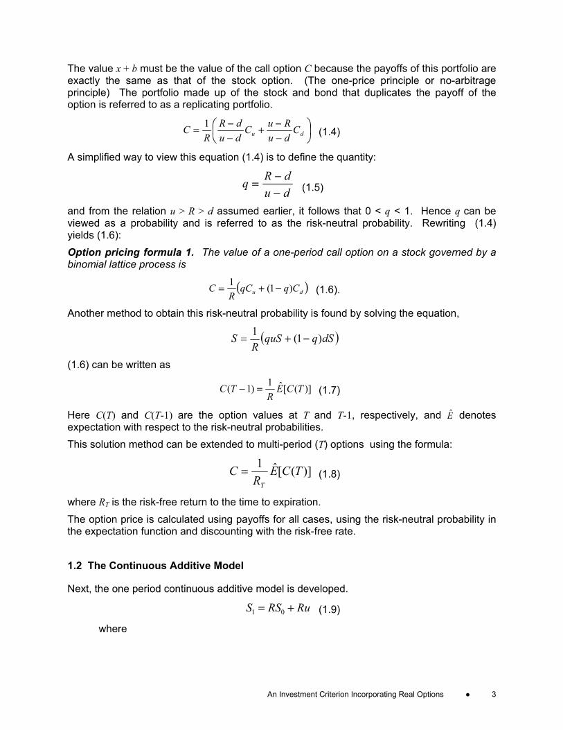
An Investment Criterion Incorporating Real Options ● 3

The value x + b must be the value of the call option C because the payoffs of this portfolio are exactly the same as that of the stock option. (The one-price principle or no-arbitrage principle) The portfolio made up of the stock and bond that duplicates the payoff of the option is referred to as a replicating portfolio.

−−

+−−

= du CduRuC

dudR

RC 1

(1.4)

A simplified way to view this equation (1.4) is to define the quantity:

dudRq

−−

= (1.5)

and from the relation u > R > d assumed earlier, it follows that 0 < q < 1. Hence q can be viewed as a probability and is referred to as the risk-neutral probability. Rewriting (1.4) yields (1.6): Option pricing formula 1. The value of a one-period call option on a stock governed by a binomial lattice process is

( )du CqqCR

C )1(1−+= (1.6).

Another method to obtain this risk-neutral probability is found by solving the equation,

( )dSqquSR

S )1(1−+=

(1.6) can be written as

)]([ˆ1)1( TCER

TC =− (1.7)

Here C(T) and C(T-1) are the option values at T and T-1, respectively, and E denotes expectation with respect to the risk-neutral probabilities. This solution method can be extended to multi-period (T) options using the formula:

)]([ˆ1 TCER

CT

= (1.8)

where RT is the risk-free return to the time to expiration. The option price is calculated using payoffs for all cases, using the risk-neutral probability in the expectation function and discounting with the risk-free rate. 1.2 The Continuous Additive Model

Next, the one period continuous additive model is developed.

RuRSS += 01 (1.9)

where


tS : stock price at time t u : normal distribution with mean 0, variance 2σ

R : Return of risk-free asset This model satisfies risk-neutral because

][][ 01 RuRSESE +=

][][ 0 RuERSE +=

0RS=

i.e. ][110 SE

RS = (1.10)

A call option on this stock with exercise price = RK at time 1, payoff of option C(1) is:

)]0,[max()1( 1 RKSC −=

i.e. 0)1( =C if RKS <1

RKSC −= 1)1( if RKS >1 (1.11)

This option price can be calculated using the general option pricing formula (1.8).

)]([ˆ1 TCER

CT

=

)]1([ˆ1 CER

=

11)()1(1 dSSfCR ∫

+∞

∞−

=

where )( 1Sf is probability density function of S1, normally distributed.

111 )()(1 dSSfRKSR RK

∫+∞

−=

substituting RuRSS += 01 , )()/1()( 1 ufRSf = , RdudS =1 ,

∫+∞

−

−+=

0

)(1)(10

SK

RduufR

RKRuRSR

[ ]∫+∞

−

−+=0

)()( 0SK

duufKuS (1.12)

Assume uSV += 0 is normally distributed with mean 0S , variance 2σ , then (1.12) can be rewritten as a general option pricing formula for continuous outcome model. Option pricing formula 2. The value of a one-period call option on a stock governed by a continuous additive model is


∫+∞

−=K

dVVfKVC )()( (1.13)

where V: the present value of the future random value discounted by risk-free rate K is the present value of exercise price, discounted by the risk-free rate This option formula will used in section 3.

Figure 1.2 Payoff and Option Price

V

Pay

off,

Opt

ion

Pric

e

Prob

abilit

y

K =Exercise Price

Density Function of V

C

Payoff=C(1)

E [V ]

Note that when V takes a lognormal distribution, this formula is equivalent to Black-Scholes call option formula (Herath and Park 2001). Following the discussion of the previous section, this model can be extended to multi-period (T) options using the model:

tt

tt uRRSS += −1 (1.14)

where iu is the random variable normally distributed with mean 0, variance 2σ

i.e. ∑=

+=T

ii

TTT uRSRS

10 (1.15)

This can be confirmed to be risk-neutral because:

01

0 ][][ SRuRESRESE TT

ii

TTT =

+= ∑

=

since 0][ =iuE for all i

i.e. ]][[][10 TTT SEPVSE

RS == .

And assuming iu is not correlated with any other iju ≠ , the variance of PV[ E[ST ] ] is:


2

1

2 ]][[ σσ TuVarSPVVarT

iiTT =

=≡ ∑

= (1.16)

or

TTσσ = (1.17)

The one-term standard deviation can be calculated from multi-term one. The standard deviation of the yearly return is called volatility.3 When the return is defined as ]/[ 0SSPV T , its volatility is given by ( 0/ Sσ ).

Although the option pricing theory has been developed in order to value financial options, it can be applied to the real asset or firm’s project. The methodology is called “real options.” The next section shows how it is applied. 2. REAL OPTIONS Real Options methodology is an approach used to evaluate alternative management strategies using traditional option-pricing theory applied to the real assets or projects. For example, when managers decide to assess a new project, they face several choices beyond simply accepting or rejecting the investment. Other choices include delaying the decision until the market is favorable, or deciding to start small and expanding later if the result seems to be superior. The traditional valuation method, DCF analysis, fails to account for these other choices. The list of these real options is shown in Table 2.1 (Alleman and Rappoport 2002)4

Table 2.1 : Description of OptionsOption Description

Defer To wait to determine if a "good" state-of-nature obtainsAbandon To obtain salvage value or opportunity cost of the assetShutdown & restart To wait for a "good" state-of-nature and re-enterTime-to-build To delay or default on project - a compound optionContract To reduce operations if state-of-nature is worse than expectedSwitch To use alternative technologies depending on input pricesExpand To expand if state-of-nature is better than expectedGrowth To take advantage of future, interrelated opportunities

Example: Value of the Option to Defer One real option alternative is the deferral option which is based on the concept of the call option, as shown in Figure 2.1 Luehrman (1998a).

3 A precise definition of volatility is “the standard deviation of the return provided by the asset in one year when the return is expressed using continuous compounding.” Hull (2003). 4 Methods to valuate each kind of option are described in several books Trigeorgis (1996), Amram and Kulatilaka (1999), Copeland and Antikarov (2001), and Copeland, Koller, and Murrin (2000).


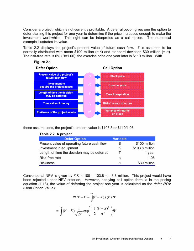
Consider a project, which is not currently profitable. A deferral option gives one the option to defer starting this project for one year to determine if the price increases enough to make the investment worthwhile. This right can be interpreted as a call option. The numerical example illustrates its value. Table 2.2 displays the project’s present value of future cash flow. V is assumed to be normally distributed with mean $100 million (= S) and standard deviation $30 million (= σ). The risk-free rate is 6% (R=1.06); the exercise price one year later is $110 million. With

Figure 2.1

Present value of a project ’s future cash flow

Investment toacquire the project assets

Length of time the decision may be deferred

Time value of money

Riskiness of the project assets

Stock price

Exercise price

Time to expiration

Risk-free rate of return

Variance of returnson stock

Defer Option Call Option

S

K

T

rf

σ2

Present value of a project ’s future cash flow

Investment toacquire the project assets

Length of time the decision may be deferred

Time value of money

Riskiness of the project assets

Time to expiration

Risk-

Defer Option Call Option

S

K

T

rf

σ2

these assumptions, the project’s present value is $103.8 or $110/1.06.

Table 2.2 A projectDefer Option Variable

Present value of operating future cash flow S $100 millionInvestment in equipment K $103.8 millionLength of time the decision may be deferred T 1 yearRisk-free rate rf 1.06Riskiness σ $30 million

Conventional NPV is given by S-K = 100 – 103.8 = - 3.8 million. This project would have been rejected under NPV criterion. However, applying call option formula in the pricing equation (1.13), the value of deferring the project one year is calculated as the defer ROV (Real Option Value):

∫+∞

−==K

dVVfKVCROV )()(

∫+∞

−−−=

K

dVSVKV 2

2)(21exp

21)(

σπ


∫+∞

−−−=

8.1032

2

30)100(

21exp

21)8.103( dVVVπ = 10.2 (2.1)

The flexibility to defer this project is valued at 10.2 million. Adding NPV and ROV gives a positive value of 6.4 (= –3.8 + 10.2). This is called Expanded NPV or ExNPV. ExNPV represents the value of this project including future flexibility (Trigeorgis 1996). Consequently, the optimum decision is to “defer,” i.e. “wait and watch the market!”

($3.80)

$10.20

$6.40

($5.00)

$0.00

$5.00

$10.00

$15.00

ExNPV NPV = conventional net present value

ROV = value to defer

Fig. 2.2 Expanded Net Present Value (ExNPV)

THE NEW DECISION MAKING CRITERION Decision under conditions of uncertainty should be made on the basis of the current state of information available to decision makers. If the expectation of the NPV were negative for the investment, the conventional approach would be to reject the investment. However, if one has the ability to delay this investment decision and wait for additional information, the option to invest later has value. This implies that the investment should not be undertaken at the present time. It leaves open the possibility of investing in future periods. For the purpose of analyzing the relationship between NPV and the option value associated with the single investment, we assume that the random variable of interest is the present value of future cash flow V, which is assumed to be normally distributed V ~ N(m’, σ’). The investment cost I is assumed to be a constant. In the conventional method, NPV is expressed as:

NPV = E [V – I] = E[V] – I

= m' - I (3.1)

Two cases are examine: Aaa ∈),( 21 are defined as Act 1: )( 1a do not invest when NPV < 0,

and Act 2: )( 2a invest when NPV > 0.


3.1 Case 1: Act 1. Do not invest as NPV < 0

Here, following Herath and Park (2001), a loss function is introduced. When no investment takes place, obviously, the cash flow is equal to 0. But imagine the situation that V > I, where the opportunity loss is recognized as V - I. Therefore the loss function of Act 1 is:

),( 1 VaL = 0 if V < I

= V - I if V > I (3.2) The expected opportunity loss can be calculated as:

∫+∞

∞−

= dVVfVaLVaLE )(),()],([ 11

∫+∞

−=I

dVVfIV )()( (3.3)

This function is the payoff of a call option, (1.11) using the pricing formula of a call option discussed in the previous section, (1.13). Assuming an investment can be deferred until new information is obtained, this value is the same as the defer option for the investment. Moreover, the value is also equal to the expected value of perfect information (EVPI) for this investment opportunity Herath and Park (2001) .

ROV = ∫+∞

−I

dVVfIV )()( (3.4)

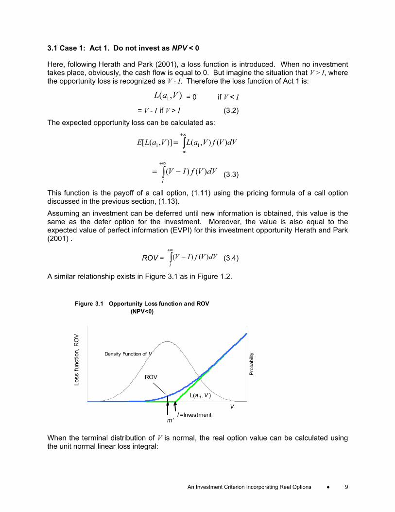
A similar relationship exists in Figure 3.1 as in Figure 1.2.

Figure 3.1 Opportunity Loss function and ROV (NPV<0)

V

Loss

func

tion,

RO

V

Prob

abilit

y

I =Investment

Density Function of V

ROV

L(a 1 ,V )

m'

When the terminal distribution of V is normal, the real option value can be calculated using the unit normal linear loss integral:


∫+∞

−=D

NN dVVfDVDL )()()( (3.5)

where fN(V) is the standard normal density function

ROV = )(' DLNσ (3.6)5

where '|'|

σImD −

=

When a manager makes an investment decision, her optimal decision is not to invest if NPV = m'-I < 0. Then she may compare the NPV and the defer option value. If she finds that the option value is larger than the absolute value of NPV (= | m'-I |), she has the option to defer and watch for positive changes in the investment opportunity. If the option value is too small to compensate the NPV (< 0), she will abandon this investment proposal. Decision Criterion 1: (Case of NPV < 0)

ROV > |NPV| → Wait and watch the opportunity carefully ROV < |NPV| → Do not invest

We can solve the equation, ROV = |NPV| (3.7)

for '|'|

σImD −

= .

From (3.1) and (3.6), (3.7) is expressed as

ImDLN −= ')('σ (3.8)

Divided by σ‘, we have: (because σ‘ > 0)

'|'|)(

σImDLN

−=

i.e. 0)( =− DDLN (3.9)

Solving this equation, D is:

0)( =− DDLN

0)()( =−−∫+∞

DdVVfDVD

N

0)()( =−− ∫∫+∞+∞

DdVVfDdVVVfD

ND

N

( ) 021exp

21 2 =−−−

− DDDD Φ

π

5 This expression is only for the case NPV < 0 though general expression is possible.


where ( ) ∫∞−

=a

N dxxfa )(Φ

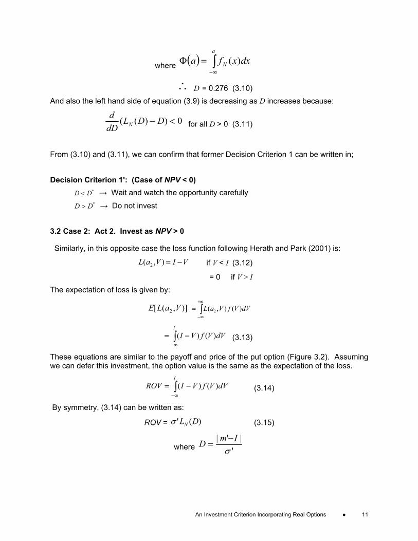
∴ D = 0.276 (3.10) And also the left hand side of equation (3.9) is decreasing as D increases because:

0))(( <− DDLdDd

N for all D > 0 (3.11)

From (3.10) and (3.11), we can confirm that former Decision Criterion 1 can be written in; Decision Criterion 1': (Case of NPV < 0)

*DD < → Wait and watch the opportunity carefully *DD > → Do not invest

3.2 Case 2: Act 2. Invest as NPV > 0

Similarly, in this opposite case the loss function following Herath and Park (2001) is:

VIVaL −=),( 2 if V < I (3.12)

= 0 if V > I The expectation of loss is given by:

)],([ 2 VaLE ∫+∞

∞−

= dVVfVaL )(),( 2

∫∞−

−=I

dVVfVI )()( (3.13)

These equations are similar to the payoff and price of the put option (Figure 3.2). Assuming we can defer this investment, the option value is the same as the expectation of the loss.

∫∞−

−=I

dVVfVIROV )()( (3.14)

By symmetry, (3.14) can be written as:

ROV = )(' DLNσ (3.15)

where '|'|

σImD −

=


Figure 3.2 Loss Function and ROV (NPV>0)

V

Loss

Fun

ctio

n an

d R

OV

I

Density Funct ion of V

ROV

L(a 2 ,V)

m'

In this case, optimal decision is invest as NPV = m'-I > 0. Comparing the NPV with the value of this option, which is same as the cost of uncertainty, a similar criterion is reached: Decision Criterion 2: (Case of NPV > 0)

ROV > |NPV| →Invest carefully ROV < |NPV| →Invest

Rewriting this as: Decision Criterion 2': (Case of NPV > 0)

*DD < → Invest carefully *DD > →Invest

Defining the decision-making index ')'( σImd −≡ , which is given from eliminating the absolute value sign from D, these two decision criteria can be combined as: Combined Decision Criterion

Invest if dD <*

Invest carefully if *0 Dd <<

Wait and watch if 0* <<− dD

Do not invest if *Dd −<

where ''σ

Imd −= , *D = 0.276

Consequently, only observing three parameters, ',' σm and I gives sufficient information to make more sophisticated decisions under uncertainty, expressing them in form of the new decision-making index, d.


3.3 Interpretation of d and D*

How can d and D* be interpreted? First, d can be seen as NPV divided by its standard deviation. In other words, d is the ratio of NPV to its uncertainty. Because d does not depend on the size of the project, it can be called “uncertainty-adjusted NPV” or “risk-normalized NPV.” Several risky projects of which the sizes are different can easily compared. Next, when d = - D*, option value to defer is equal to expected loss of

Figure 3.3 Summary of the CriterionNPVROV |NPV| > ROV |NPV| < ROV

d d < -D* -D* < d < 0Decision not Invest wait and watch

NPVROV |NPV| < ROV |NPV| > ROV

d 0 < d < D* D* < d

Decision Invest carefully Invest

NPV < 0

NPV > 0

V

ROV

E[NPV]=m'-I V

ROV

E[NPV]=m'-I

V

ROV

E[NPV]=m'-IV

ROV

E[NPV]=m'-I

NPV, namely, D* is the break-even point of expectation of NPV and its option value, or the point where ExNPV = 0. What is the probability that the payoff of this defer option is positive if d = -D* at time 0? This can be calculated as follows,

>

′−

=>− 0]0[σ

IVPIVP

>

′−′+′−

= 0σ

ImmVP


′−′

−>′

′−=

σσImmVP

[ ]dNP −>=

[ ]*DNP >=

= .39

where N is standard normal distribution.

Because V is N ~ (m’, σ‘), (V-m’)/ σ‘ is N~ (0, 1). Therefore, the probability that the payoff of the defer option is positive is 39%. Does it seem to be a high probability to abandon this option? Yes, it does! The criterion d < -D* means, “Do not invest now” but does not mean “Abandon the defer option.” The defer option itself has value though the expectation of NPV is deeply negative. If holding the option does not require any cost, it does not have to be thrown it away! Just wait and watch what happens in the next period. On the other hand, if d = D*, the probability that the project will be out of the money is also 39%, by symmetry. When the manager makes her decision to invest as d = D*, there is still 39% probability of losing money. If the manager wanted a positive NPV with probability 90%, d should be higher than 1.28. It might be the case that the manager could set a higher d for the decision criterion if she would not care about opportunity losses. The tradeoffs between opportunity loss and cost of uncertainty are shown in Figure 3.4 In the next section, shows an example of this criterion.

Figure 3.4 Tradeoffs of Losses

-2 -1 0 1 2d

Loss

0

0.2

0.4

0.6

0.8

1

Prob

abilit

y

Probability Payoff > 0

Expected Opportunity Loss

D *-D *

Expected Loss


EXAMPLE CASES Six Independent Projects

Consider the projects shown in Table 4.1, How can decisions be made using the new criterion? The assets that have current value S, time to expiration T, exercise price K at time T, volatility σ, and risk-free rate rf. To calculate d, we have to solve m’, I and σ’. Assuming the value of S at time T is normally distributed with mean S(1+ rf)T, m’ = S because m’ is

expressed in present value. After setting I = PV(K) = K/(1+ rf)T, and, TSσ=′σ , d = (V-m’)/ σ‘ can be calculated. Therefore, d can be calculated for each project and make decision to invest as shown in Table 4.1. Luehrman (1998a and 1998b) defined “option space” having two axes value-to-cost (S/PV(K))

and volatility ( Tσ ) and showed that decision criterion depends on the region in the option space. Using his example, similar results can be found with the new criterion. The new decision criterion can is an integrated, simplified version of Luehrman’s method. Furthermore, project “E” in Table 4.1 is what was illustrated before in section 2. The new criterion gives the same decision, “wait and watch”!

Table 4.1 Valuation for Six Independent ProjectsVariable A B C D E F

S $100.00 $100.00 $100.00 $100.00 $100.00 $100.00K T $90.00 $90.00 $110.00 $110.00 $110.00 $110.00T 0.0 2.0 0.0 0.5 1.0 2.0s 30% 30% 30% 20% 30% 40%r f 6% 6% 6% 6% 6% 6%

$0.00 $42.43 $0.00 $14.14 $30.00 $56.57S-PV(K) $10.00 $19.90 -$10.00 -$6.84 -$3.77 $2.10

d +infinite 0.469 -infinite -0.484 -0.126 0.037

Exercise decision invest invest do not

investdo not invest

wait and watch

invest carefully

S Current asset valueK T Exercise Price (at time = T)T Time to expiration (year)s Standard deviation of return (per year)r f Risk-free rate of return (% per year)

CONCLUSION Applying real option valuation methodology shows that the new decision index d – the uncertainty adjusted NPV – and D* = 0.276 – the break-even point of NPV and ROV (real option value) – gives a clear solution to make a decision under uncertainty. When making decision, managers have to observe only three parameters: expectation of future cash flow,


its uncertainty, and the amount of investment to acquire the project. The examples using the new criterion show its usefulness. REFERENCES: Alleman, James and Eli Noam (eds.). The New Investment Theory of Real Options and Its Implication for Telecommunications Economics, Kluwer Academic, 1999 Alleman, James and Paul Rappoport. Modelling Regulatory Distortions with Real Options, The Engineering Economist, volume 47, number 4, 2002, pp. 390-417. Amram, Martha and Nalin Kulatilaka. Real Options, HBS Press, 1999 Boer, Peter. The Real Options Solution: Finding Total Value in a High-risk World, John Wiley & Sons, Inc. 2002 Damodaran, Aswath. Dark Side of Valuation, Prentice-Hall, 2001 Dixit, Avinash and Robert Pindyck. Investment Under Uncertainty, Princeton University Press, 1994 Copeland, Tom and Vladimir Antikarov. Real Options: A Practitioner’s Guide, Texere LLC, 2001 Copeland, Tom, Tim Koller, and Jack Murrin. Valuation: Measuring and Managing the Value of Companies, McKinsey & Company Inc Herath, Hemantha and Chan Park. Real Options Valuation and Its Relationship to Bayesian Decision-Making Methods, The Engineering Economist 2001, Vol. 46, No.1 Hull, John. Options, Futures and other Derivatives, Fifth Edition, Prentice-Hall, 2003 Luehrman, Timothy. Investment Opportunities as Real Options: Harvard Business Review, 51-67, July-August 1998a Luehrman, Timothy. Strategy as a Portfolio of Real Options: Harvard Business Review, 89-99, September-October 1998bDavid G. Luenberger, David. Investment Science, Oxford University Press, 1998 Mauboussin, Michael. Get Real, Credit Suisse Equity Research, June 1999 Nembhard, Harriet, Leyuan Shi, and Chan Park. Real Option Models For Managing Manufacturing System Changes in The New Economy, The Engineering Economist 2000, Vol.45, No.3 Schlaifer, Robert. Introduction to Statistics for Business Decisions, McGraw Hill, 1961 Smith, James and Robert Nau, Valuing Risky Projects: Option Pricing Theory and Decision Analysis, Management Science Vol. 41, No.5, May 1995 Trigeorgis, Lenos. Real Options: Managerial flexibility and strategy in resource allocation, MIT Press, 1996 Yamamoto, Daisuke. Introduction to Real Options, Toyo-Keizai, 2001 (in Japanese)

An Investment Criterion Incorporating Real Options

Documents

Transcript of An Investment Criterion Incorporating Real Options