Multiscale Discrete Geometry

Multiscale Discrete Geometry

Mouhammad Said12, Jacques-Olivier Lachaud1, Fabien Feschet2

1 Laboratoire de Mathematiques, UMR 5127 CNRS, Universite de Savoie,73376 Le Bourget du Lac, France

[email protected], [email protected]

2LAIC, Univ. Clermont-Ferrand,IUT, Campus des Cezeaux, 63172 Aubiere Cedex, France

[email protected]

Abstract. This paper presents a first step in analyzing how digitalshapes behave with respect to multiresolution. We first present an analy-sis of the covering of a standard digital straight line by a multi-resolutiongrid. We then study the multi-resolution of Digital Straight Segments(DSS): we provide a sublinear algorithm computing the exact charac-teristics of a DSS whenever it is a subset of a known standard line. Wefinally deduce an algorithm for computing a multiscale representation ofa digital shape, based only on a DSS decomposition of its boundary.

Key words: multiscale geometry, digital contours, standard lines, dig-ital straight segment recognition, Stern-Brocot tree, multi-resolution

1 Introduction

Multiscale analysis is a classical tool in image processing [15, 11]. It has beenintroduced for addressing the fact that derivatives or geometric features are sen-sitive to the notion of scale. They do not intrinsically exist but they are oftenpresent only at a finite number of scales. To compute this representation, theoriginal signal is embedded in a parameterized family of derived signals, obtainedby convolutions of a parameterized family of Gaussian kernels, whose variance isthe scale. At any scale, smooth versions of the derivatives are computed. Com-bined together, they provide a multiscale representation of the feature geometry,thus providing information about its significance for later interpretation or post-processing. Originally defined in the continuous space, these approaches havebeen extended to the discrete case [13] to better handle both the finite supportand the finite resolution of digital images.

The use of Gaussian convolutions does not process well binary data such asdigital curves. So, another approach must be followed. We can consider theapproach of Vacavant et al. [14] as a multiscale approach in the sense thatgeometric objects are represented by a multi-resolution set of rectilinear tiles.However, the set of tiles is not intrinsic and is computed from the digital objectsas the result of an optimization process. Indeed, they determine the minimalnumber of rectangles whose union covers the considered object. In this way,

2 Mouhammad Said12, Jacques-Olivier Lachaud1, Fabien Feschet2

they define geometric primitives such as lines and use them to analyze thickdigital objects. Its potential is yet unclear for multiscale analysis of digital objectfeatures, and the constructed objects are not analytically defined.

We believe that, in the context of digital geometry, geometric primitives suchas lines, circles or polynomials are of a great importance. Pieces of digital linesare excellent tangent estimators [7, 12], circular arcs estimate curvature [1]. It isthus fundamental to keep them in the multiscale analysis of digital boundaries.Our point of view is therefore similar to the one of Figueiredo [8] who studiedthe behavior of 8-connected lines when changing the resolution of the grid. Hewas the first to characterize when the image of such a digital line in variousresolution grids is another digital line.

In the present paper, we pursue on this idea and we provide in Section 2an analytic description of how 4-connected digital straight lines, called digitalstandard lines (DSL), behave when the resolution of the grid is changed by anarbitrary factor. We prove first that their subsampling is also a standard line,whose parameters can all be analytically defined (Theorems 1 and 2).

The multiresolution of a digital straight segment (DSS) is addressed in Sec-tion 3. However, a full analytic approach seems out of reach at the moment. Thisis why we take an algorithmic approach. We present a new algorithm which com-putes the exact characteristics of a DSS that is a subset of a known DSL, giventhe endpoints of the DSS. Not surprisingly, it is based on continued fractions.Its worst-case computational complexity is Θ(

∑ki=0 ui), where [u0;u1, . . . , uk] is

the continued fraction of the slope of the input DSL. The expectation of thissum for fractions a

b with a+ b = n is experimentally lower than log2 n, and thissum is upper bounded by n. This is to compare with classical DSS recognitionalgorithms (e.g., see [4]), whose complexities are at best Θ(n).

Section 4 applies the preceding results to the multiscale computation of adigital shape. We show there that if the digital shape was previously polygo-nalized as a sequence of M DSS, its exact multiresolution is computed in timelinear with M times the average of the sums of the partial cofficients of its outputDSS slopes. In most cases, this is clearly sublinear, and at worst, linear in thesize of the contour. This paper is therefore a first step towards the multiscalecomputation of the tangential cover [6, 12], a fundamental tool for representingand analyzing digital curves.

2 Covering of a standard line by a lower resolution grid

A first step for defining multiscale discrete geometry is to find the coveringof a digital straight line by a lower resolution grid. We shall prove here thatthis covering is indeed a digital straight line with computable characteristics(Theorem 1) and that this line is standard (Theorem 2). The proof is essentiallytechnical and is based on the same principle as the proof of Figueiredo [8].

Let D(a, b, µ) be a standard digital line such that 0 < a < b and gcd(a, b)=1.Let us consider the subgroup S(h, v)= (Xh, Y v) of Z2 (where X, Y , h, v allare integers). Obviously the fondamental domain [0, h)× [0, v) of S(h, v) and its

Multiscale Discrete Geometry 3

translations by the vectors X(h, 0) + Y (0, v) induce a tiling of Z2 where each tilecontains exactly one point of S(h, v) (for which reason we will refer indifferentlyto the tile itself or to the point of S(h, v) it contains). We are interested in theset of tiles of S(h, v) that intersect D(a, b, µ). The set of tiles is a discrete linein the subgroup S(h, v). We denote this line by ∆ and call it the covering lineof D(a, b, µ) in S(h, v).

The tiling generated by S(h, v) on Z2 induces a new coordinate system wherecoordinates (X,Y ) are related to the canonical coordinates of Z2 by the followingobvious relations where

[xh

]is the quotient of the euclidean division of x by h

and{xh

}is the remainder of this division:

X =[xh

]Y =

[yv

]x = hX +

{xh

}y = vY +

{yv

}.

By definition, D(a, b, µ) can be written as

µ ≤ ax+ by < µ+ a+ b (1)

Hence the equation of ∆ in the coordinate system related to S writes:

µ ≤ a(hX +{xh

}) + b(vY +

{yv

}) < µ+ a+ b (2)

In order to simplify (2) let us introduce

mx ={xh

}my =

{yv

}(3)

Since mx and my vary when x steps through Z, equation (2) becomes:

µ−maxx∈Z

(amx + bmy) ≤ ahX + bvY < µ+ a+ b−minx∈Z

(amx + bmy) (4)

Now to fully determine this equation that defines the covering of the digital lineby the tiling, the exact range of amx+bmy, i.e, the values of minx∈Z(amx+bmy)and maxx∈Z(amx + bmy), need to be calculated.

By definition of mx and my, we have 0 ≤ mx ≤ h − 1 and 0 ≤ my ≤ v − 1.Using these bounds in (4) suggests for ∆ an equation of the form:

µ− a(h− 1)− b(v − 1) ≤ ahX + bvY < µ+ a+ b. (5)

But since ahX+bvY can only assume values that are multiples of g = gcd(ah, bv),the bounds of equation (4) can be refined. We further denote ah+bv

g by p.

However since mx and my are linked through (2) and (3), the precise bounds ofamx + bmy when x steps through Z, need to be determined. In fact, we show inwhat follows, that even though amx + bmy does not reach the absolute bounds0 and a(h− 1) + b(v − 1) in some cases, equation (20) (given on page 6) alwaysholds.Inverting (3) yields x = kh + mx, k ∈ Z and y = lv + my, l ∈ Z. Hence, afterinsertion into (1):

µ− akh− blv ≤ amx + bmy < µ+ a+ b− akh− blv (6)


1 2 3 4 5

0

1

2

3

4

5

0

Fig. 1. Determination of the range of 2mx+3my. The black squares represent thefamily of standard digital lines defined by 5− 6t ≤ 2mx + 3my < 10− 6t restricted to[0, 6)× [0, 6) and hence the possible values of (mx,my)

The term akh + blv has values which are multiples of g. Equation (6) can thusbe rewritten as

µ− tg ≤ amx + bmy < µ+ a+ b− tg, t ∈ Z (7)

Equation (7) describes a family of digital lines of direction (a, b) parameterizedby t ∈ Z, which we denote by Dt. The intersection of Dt with the domain of(mx,my), [0, h) × [0, v) defines the possible pairs (mx,my) and therefore therange of possible values for the sum amx + bmy (see Figure 1).

Let us denote with (nx, ny) the pair of Dt ∩ [0, h) × [0, v) that yields themaximum value for the sum amx + bmy. Let us also denote by d the differencebetween amx + bmy evaluated at (h− 1, v − 1) and at (nx, ny):

d = a(h− 1) + b(v − 1)− (anx + bny) (8)

Determining the maximum value of t verifying (7) for the point (nx, ny)provides a more precise expression of the lower bound of d. (8) becomes

d = (p+ t)g − (µ+ 2a+ 2b− 1).

To find the maximum value, we take d = 0 which implies that (nx, ny) =(h− 1, v − 1), and

t = −p+Q2 +R2

g, (9)

where Q2 =[µ+2a+2b−1

g

]and R2 =

{µ+2a+2b−1

g

}. Now, we must distinguish

two possible cases for R2.


1. If g divides µ + 2a + 2b − 1. In this case, (9) becomes t = −p + Q2 and weinsert this equality in (4).

ahX + bvY ≥ µ−maxx∈Z

(amx + bmy) ≥ (−p+Q2) g − a− b+ 1

Let α = ahg and β = bv

g . Then the previous equation can be rewritten as:

αX + βY ≥ −p+Q2 −Q1 (10)

where Q1 =[a+b−1g

]and R1 =

{a+b−1g

}.

2. If g does not divide µ+ 2a+ 2b−1. In this case, we insert (9) directly in (4).

αX + βY ≥ −p+Q2 −Q1 +R2

g− R1

g

We calculate the difference between the division of R2 by g and the divisionof R1 by g, by comparing R1 and R2:

If R2 ≤ R1, then αX + βY ≥ −p+Q2 −Q1 (11)

If R2 > R1, then αX + βY ≥ −p+Q2 −Q1 + 1 (12)

A similar reasoning can be applied with the minimum value of amx + bmy

throughout Dt ∩ [0, h)× [0, v) obtained at point (n′x, n′y). Let us also denote by

d′ the difference between amx + bmy evaluated at 0 and at (n′x, n′y):

d′ = 0− (an′x + bn′y). (13)

Determining the maximum value of t verifying (7) for the point (n′x, n′y) provides

a more precise expression of the upper bound of d′. (13) becomes

d′ = 0− (µ− tg) = (µ+ 2a+ 2b− 1) + tg − (2µ+ 2a+ 2b− 1)

We take d′ = 0 to find the minimum value, implying (n′x, n′y) = (0, 0), then:

t = −Q2 −R2

g+

(2µ+ 2a+ 2b− 1

g

)(14)

At this point, we must distinguish two possible cases according to R2.

1. If g divides µ+2a+2b−1. In this case, (14) becomes t = −Q2+(

2µ+2a+2b−1g

)and we insert this equality in (4):

ahX + bvY < µ+ a+ b− (µ− tg) < −Q2g + 2µ+ 3a+ 3b− 1

and,

αX + βY < −Q2 +Q3 +R3

g, (15)

where Q3 =[2µ+3a+3b−1

g

]and R3 =

{2µ+3a+3b−1

g

}.

We must further distinguish two possible cases for R3.


(a) If g divides 2µ+ 3a+ 3b− 1. In this case Equation (15) becomes

αX + βY < −Q2 +Q3. (16)

(b) If g does not divide 2µ+ 3a+ 3b− 1. In this case Equation (15) becomes

αX + βY < −Q2 +Q3 + 1. (17)

2. If g does not divide µ + 2a + 2b − 1. In this case we insert (14) directly in(4):

ahX + bvY < µ+ a+ b− (µ− tg) < −Q2g −Q1 + 2µ+ 3a+ 3b− 1.

Then the previous equation can be rewritten as:

αX + βY < Q3 −Q2 +R3

g− R2

g.

We calculate the difference between the division of R3 by g and the divisionof R2 by g, by comparing R2 and R3:

If R3 ≤ R2, then αX + βY < −Q2 +Q3 (18)

If R3 > R2, then αX + βY < −Q2 +Q3 + 1 (19)

More precisely, eleven equations involving αX + βY can be obtained bycombining the lower bound (equations (10), (11), (12)) and the upper bound(equations (16), (17), (18), (19)) of αX + βY . Among the eleven possible cases,four cases are impossible. For the remaining cases we have also conditions whichyield the same result. Therefore those equations can be formulated as a singleexpression given below.

Theorem 1 The digital straight line ∆ of S(h, v) covering the standard digitalline D(a, b, µ) of Z2 is defined by:

−p+Q2 −Q1 + SI ≤ αX + βY < Q3 −Q2 + SS (20)

Where α = ahg , β = bv

g , g = gcd(ah, bv), p = α+ β and

SI =

{0 if R2 ≤ R1

1 otherwiseSS =

{0 if R3 ≤ R2

1 otherwise

Figure 2 illustrates the covering of D(7, 9, 6) in the subsampling (6, 6).

Theorem 2 The covering line ∆ is standard.

In order to prove that the difference between the upper and lower bounds of(20) is equal to α+ β, we first need the following proposition and lemma.


-42

-36

-30

-24

-18

-12

-6

0

6

12

18

24

30

36

42

-54 -48 -42 -36 -30 -24 -18 -12 -6 0 6 12 18 24 30 36 42 48 54 60

Standard Digital LineCovering of Standard Digital Line

Fig. 2. The covering line of D(7, 9, 6) by S(6, 6) : −12 ≤ 7X + 9Y < 4

Proposition 1

R2−R1−Rg =

{0 if R1 ≤ R2

−1 otherwise.and R3−R2−R

g =

{0 if R2 ≤ R3

−1 otherwise.

Proof. Since 0 ≤ R1 < g, 0 ≤ R2 < g and 0 ≤ R < g, then 0 ≤ R1

g < 1,

0 ≤ R2

g < 1 and 0 ≤ Rg < 1. Thus we can write −2 < R2−R1−R

g < 1. To specify

the exact integer value of R2−R1−Rg , we must compare R1 and R2.

– If R1 ≤ R2, then R2 = (µ+ 2a+ 2b− 1) mod g = (µ+ a+ b) mod g + (a+b− 1) mod g = R+R1. Therefore R2 −R1 −R = 0 and R2−R1−R

g = 0.

– If R1 > R2, then R2 = (µ+2a+2b−1) mod g = (µ+a+b) mod g+(a+b−1) mod g−g = R+R1−g. Therefore R2−R1−R = −g and R2−R1−R

g = −1.The proof of the second condition is analogous to the first one. ut

Lemma 1

Q2 −Q1 = Q+

{0 if R1 ≤ R2

1 otherwise.and Q3 −Q2 = Q+

{0 if R2 ≤ R3

1 otherwise.

Proof. We only provide the proof of the first result and the second result has asimilar proof, µ+ a+ b = (µ+ 2a+ 2b− 1)− (a+ b− 1), then by definition ofthe Euclidean division, we can write µ+ a+ b = gQ+R, a+ b− 1 = gQ1 +R1,and µ + 2a + 2b − 1 = gQ2 + R2. So, the first equality can be rewritten asgQ+R = (gQ2 +R2)− (gQ1 +R1). Then,

g(Q−Q2 +Q1) = R2 −R1 −R

To reduce this equality, we must compare R1 and R2

1. If R1 ≤ R2, then by Proposition 1, R2−R1−Rg = 0 which implies that Q =

Q2 −Q1,


2. If R1 > R2, then by Proposition 1, R2−R1−Rg = −1 which implies that

Q = Q2 −Q1 − 1.

ut

Proof (Theorem 2). We want to prove that the difference between the upperand lower bounds of (20) is equal to α+ β. There are 5 cases to consider. FromProposition 1 and Lemma 1, we get:

– If R3 < R2 < R1, then SI = 0, SS = 0, Q2−Q1 = Q+1 and Q3−Q2 = Q+1.

– If R2 < R1 and R2 < R3, then SI = 0, SS = 1, Q2 − Q1 = Q + 1 andQ3 −Q2 = Q.

– If R1 < R2 < R3, then SI = 1, SS = 1, Q2 −Q1 = Q and Q3 −Q2 = Q.

– If R1 < R2 and R3 < R2, then SI = 1, SS = 0, Q2 − Q1 = Q andQ3 −Q2 = Q+ 1.

– If R1 = R2 = R3, then SI = 0, SS = 0, Q2 −Q1 = Q and Q3 −Q2 = Q.

It is easy to see for all cases that, (Q3 −Q2 + SS)− (−p+Q2 −Q1 + SI) = p.ut

3 A fast DSS recognition Algorithm

We focus now our attention on the multiresolution of digital straight segments(DSS), which are finite connected parts of digital lines. In the first subsection,we recall first some links between DSS, patterns, continued fraction of the slope,and Stern-Brocot tree representation of fractions. Let S be some DSS includedin a line D. We then obtain easily Proposition 3, which states that the slopeof the (h, v)-multiresolution S′ of S is some reduced fraction of the slope of the(h, v)-multiresolution D′ of D. However, the full analytic description of S′ seemsout of reach at the moment. This is why we propose an algorithmic approach inthe second subsection. All the characteristics of S′ can be determined in timesublinear in the number of points of S′ (Algorithm 2 and Proposition 4).

3.1 DSS, patterns, irreducible fractions and continued fractions

Given a standard line (a, b, µ), we call pattern of characteristics (a, b) the suc-cession of Freeman moves between any two consecutive upper leaning points.The Freeman moves defined between any two consecutive lower leaning pointsis the previous word read from back to front and is called the reversed pattern.As noted by several authors (e.g. see [10], or the work of Berstel reported in [2]),the pattern of any slope can be constructed from the continued fraction of theslope. We recall that a simple continued fraction is an expression:

z = ab = [u0, u1, u2, ..., ui, ..., un] = u0 + 1

u1+1

...+ 1un−1+ 1

un

,


where n is the depth of the fraction, and u0, u1, etc, are all integers and called thepartial quotients. We call k-th convergent the simple continued fraction formedof the k first partial quotients: zk = pk

qk= [u0, u1, u2, ..., uk].

The role of partial quotients can be visualized with a structure called Stern-Brocot tree (see [9] for a complete definition) which is a hierarchy containingall the positive irreductible rational fractions. The idea under its constructionis to begin with the two fractions 0

1 and 10 and to repeat the insertion of the

median of these two fractions as follows: insert the median m+m′

n+n′ between mn

and m′

n′ . The sequence of partial quotients defines the sequence of right and leftmoves down the tree. Many works deal with the relations between irreduciblerational fractions and digital lines (see [5] for characterization with Farey series,and [16] for a link with decomposition into continuous fractions). In [3], Debledand Reveilles first introduced the link between this tree and the recognition ofdigital line. Recognizing a piece of digital line is like going down the Stern-Brocottree up to the directional vector of the line. To sum up, the classical online DSSrecognition algorithm DR95 [3] (reported in [10]) updates the DSS slope whenadding a point that is just exterior to the current line (weak exterior points).The slope evolution is analytically given by next property.

Proposition 2 [2] The slope evolution in DR95 depends on the parity of thedepth of its slope, the type of weakly exterior point added to the right. This issummed up in the table below, where the slope is [0, u1, ..., uk], k = 2i even ork = 2i+ 1 odd, δ pattern(s) and δ′ reversed pattern(s):

Even k Odd kUpper weakly exterior [0, u1, ..., u2i, δ] [0, u1, ..., u2i+1 − 1, 1, δ]Lower weakly exterior [0, u1, ..., u2i − 1, 1, δ′] [0, u1, ..., u2i+1, δ

′]

A slope evolution during recognition is then clearly equivalent to descendingin the Stern-Brocot tree, to the left or to the right. Since S′ is a piece of a DSLof slope a′

b′ , we therefore obtain:

Proposition 3 If D′(a′, b′, µ′) is the covering of some digital line D by a tilingS(h, v), then any segment S ⊂ D induces a segment S′ ⊂ D′ by the same tiling,

such that the slope of S′ is a′

b′ or one of its ancestors in the Stern-Brocot tree.

3.2 Fast DSS recognition when DSL container is known

We provide a general algorithmic solution to the multiresolution of a DSS thatis sublinear in the number of its points (Algorithm 2). We exploit the fact thatin our case, we know that it is a piece of a standard digital line of known charac-teristics (with Theorems 1 and 2). Therefore most of the points tested in DR95are useless since they do not lead to any slope evolution. Proposition 3 tells usthat we must find the slope of S′ in the ancestors of the slope of D′. We mustalso determine the shift to origin of S′.

Starting from the initial correct quadrant, Algorithm 2 determines progres-sively the positions of the weakly exterior points. They are related to the Bezout


coefficient of the current DSS slope pkqk

(line 1). Since we update at each step the

continued fraction of the slope, these coefficients are given in O(1) time by theformula

Bezout(p, q, k) =

{(qk − qk−1, pk − pk−1),when k is even(qk−1, pk−1),when k is odd

.

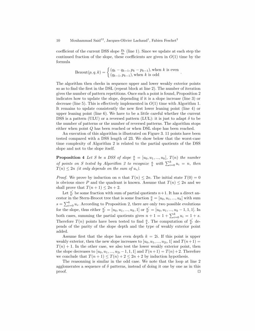
The algorithm then checks in sequence upper and lower weakly exterior pointsso as to find the first in the DSL (repeat block at line 2). The number of iterationgives the number of pattern repetitions. Once such a point is found, Proposition 2indicates how to update the slope, depending if it is a slope increase (line 3) ordecrease (line 5). This is effectively implemented in O(1) time with Algorithm 1.It remains to update consistently the new first lower leaning point (line 4) orupper leaning point (line 6). We have to be a little careful whether the currentDSS is a pattern (ULU) or a reversed pattern (LUL): it is just to adapt δ to bethe number of patterns or the number of reversed patterns. The algorithm stopseither when point Q has been reached or when DSL slope has been reached.

An execution of this algorithm is illustrated on Figure 3. 11 points have beentested compared with a DSS length of 23. We show below that the worst-casetime complexity of Algorithm 2 is related to the partial quotients of the DSSslope and not to the slope itself.

Proposition 4 Let S be a DSS of slope ab = [u0, u1, ..., uk], T (n) the number

of points on S tested by Algorithm 2 to recognize ab with

∑ki=0 ui = n, then

T (n) ≤ 2n (it only depends on the sum of ui).

Proof. We prove by induction on n that T (n) ≤ 2n. The initial state T (0) = 0is obvious since P and the quadrant is known. Assume that T (n) ≤ 2n and weshall prove that T (n+ 1) ≤ 2n+ 2.

Let a′

b′ be some fraction with sum of partial quotients n+1. It has a direct an-cestor in the Stern-Brocot tree that is some fraction a

b = [u0, u1, ..., uk] with sum

s =∑ki=0 ui. According to Proposition 2, there are only two possible evolutions

for the slope, thus either a′

b′ = [u0, u1, ..., uk, 1] or a′

b′ = [u0, u1, ..., uk − 1, 1, 1]. In

both cases, summing the partial quotients gives n + 1 = 1 +∑ki=0 ui = 1 + s.

Therefore T (n) points have been tested to find ab . The computation of a′

b′ de-pends of the parity of the slope depth and the type of weakly exterior pointadded.

Assume first that the slope has even depth k = 2i. If this point is upperweakly exterior, then the new slope increases to [u0, u1, ..., u2i, 1] and T (n+1) =T (n) + 1. In the other case, we also test the lower weakly exterior point, thenthe slope decreases to [u0, u1, ..., u2i−1, 1, 1] and T (n+1) = T (n)+2. Thereforewe conclude that T (n+ 1) ≤ T (n) + 2 ≤ 2n+ 2 by induction hypothesis.

The reasonning is similar in the odd case. We note that the loop at line 2agglomerates a sequence of δ patterns, instead of doing it one by one as in thisproof. ut


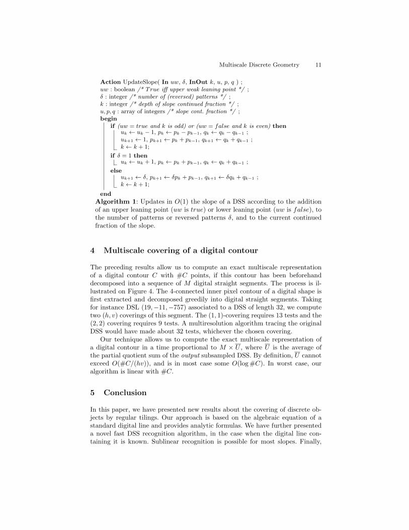
Action UpdateSlope( In uw, δ, InOut k, u, p, q ) ;uw : boolean /* True iff upper weak leaning point */ ;δ : integer /* number of (reversed) patterns */ ;k : integer /* depth of slope continued fraction */ ;u, p, q : array of integers /* slope cont. fraction */ ;begin

if (uw = true and k is odd) or (uw = false and k is even) thenuk ← uk − 1, pk ← pk − pk−1, qk ← qk − qk−1 ;uk+1 ← 1, pk+1 ← pk + pk−1, qk+1 ← qk + qk−1 ;k ← k + 1;

if δ = 1 thenuk ← uk + 1, pk ← pk + pk−1, qk ← qk + qk−1 ;

elseuk+1 ← δ, pk+1 ← δpk + pk−1, qk+1 ← δqk + qk−1 ;k ← k + 1;

end

Algorithm 1: Updates in O(1) the slope of a DSS according to the additionof an upper leaning point (uw is true) or lower leaning point (uw is false), tothe number of patterns or reversed patterns δ, and to the current continuedfraction of the slope.

4 Multiscale covering of a digital contour

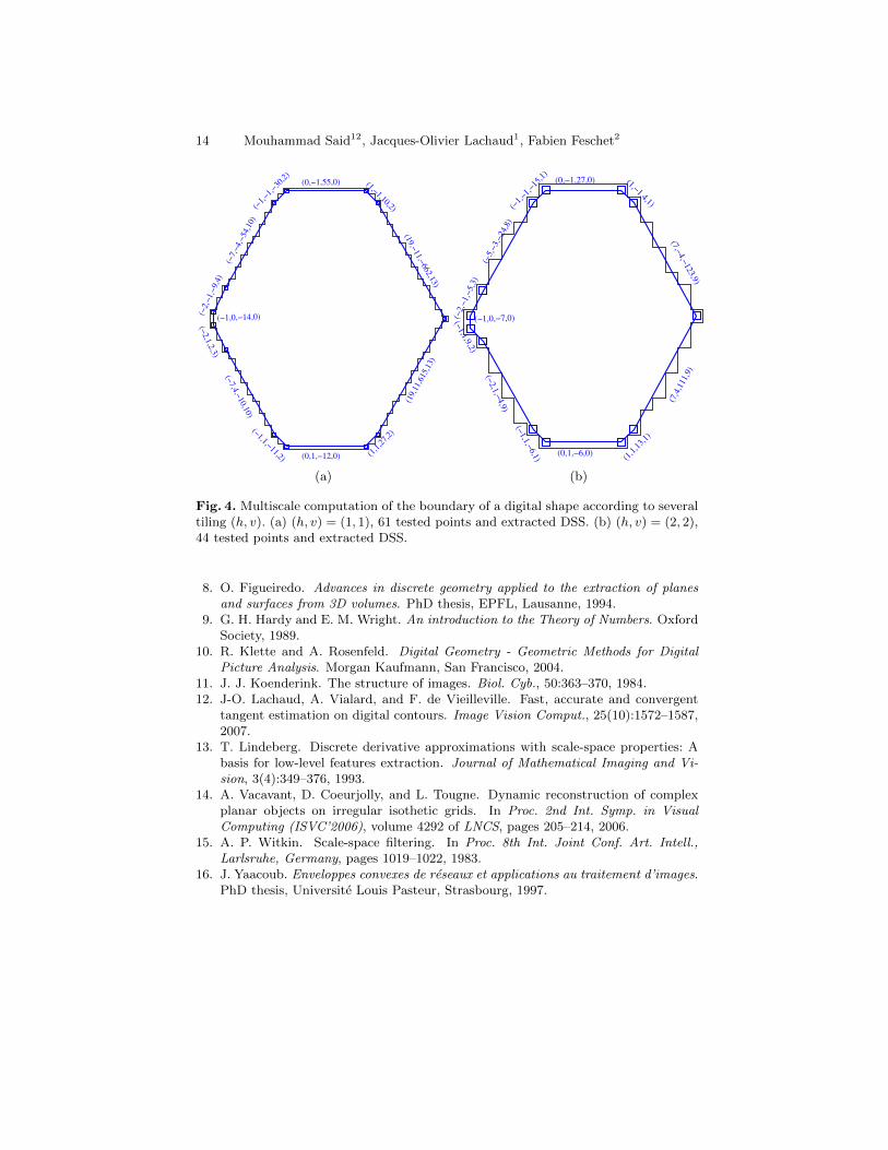
The preceding results allow us to compute an exact multiscale representationof a digital contour C with #C points, if this contour has been beforehanddecomposed into a sequence of M digital straight segments. The process is il-lustrated on Figure 4. The 4-connected inner pixel contour of a digital shape isfirst extracted and decomposed greedily into digital straight segments. Takingfor instance DSL (19,−11,−757) associated to a DSS of length 32, we computetwo (h, v) coverings of this segment. The (1, 1)-covering requires 13 tests and the(2, 2) covering requires 9 tests. A multiresolution algorithm tracing the originalDSS would have made about 32 tests, whichever the chosen covering.

Our technique allows us to compute the exact multiscale representation ofa digital contour in a time proportional to M × U , where U is the average ofthe partial quotient sum of the output subsampled DSS. By definition, U cannotexceed O(#C/(hv)), and is in most case some O(log #C). In worst case, ouralgorithm is linear with #C.

5 Conclusion

In this paper, we have presented new results about the covering of discrete ob-jects by regular tilings. Our approach is based on the algebraic equation of astandard digital line and provides analytic formulas. We have further presenteda novel fast DSS recognition algorithm, in the case when the digital line con-taining it is known. Sublinear recognition is possible for most slopes. Finally,


Action SmartDSS( In D, In P,Q, Out S ) ;D : DSL (α, β, µ′), P,Q : Point of Z2, S : DSS (a, b, µ) ;Var u, p, q : array of integers /* Cont. fraction a

b= [u0, . . . , uk] = pk

qk*/ ;

Var U,L, U ′, L′ : Point of Z2 ;Var ulu, lul, inside : boolean ;Var k, loop : integer ;begin

k ← 0, u0 ← 0, p0 ← 0, q0 ← 1, p−1 ← 1, q−1 ← 0 ;U ← P , L← P ;inside← true, ulu← true, lul← true ;while inside and pk 6= α do

(a, b)← (pk, qk) ;(b′, a′)← Bezout(p, q, k) /* ab′ − ba′ = 1 */ ;1

U ′ ← U + (b− b′, a− a′);L′ ← L+ (b′, a′);δ ← 1, loop← 0;repeat2

U ′ ← U ′ + (b, a), L′ ← L′ + (b, a);if U ′y ≤ Qy and U ′ ∈ D then loop← 1 ;else if L′x ≤ Qx and L′ ∈ D then loop← 2 ;else δ ← δ + 1 ;

until loop 6= 0 or U ′y ≥ Qy or L′x ≥ Qx ;if loop = 1 then3

/* Increase slope with weak upper leaning point U ′ */ ;UpdateSlope(true, δ, k, u, p, q ) ;L← L′ − (b′, a′) ;4

if not lul then L← L− (b, a);ulu← true, lul← false ;

if loop = 2 then5

/* Decrease slope with weak lower leaning point L′ */ ;UpdateSlope(false, δ, k, u, p, q) ;U ← U ′ − (b− b′, a− a′) ;6

if not ulu then U ← U − (b, a);ulu← false, lul← true ;

elseinside← false;

a← pk, b← qk, µ← aUx − bUy ;end

Algorithm 2: Computes the characteristics (a, b, µ) of a DSS that is somesubset of a DSL D, given a starting point P and an ending point Q (P,Q ∈ D).

The computation time is linear with the sum∑ki=0 uk with a

b = [u0, . . . , uk].


Lower leaning points

Tested points

Upper leaning points

Origin

Accepted points

Origin

Endpoints

Fig. 3. A digital straight line D(13, 17,−5) with an odd slope. Computes the charac-teristics (a, b, µ) of a DSS S that is the subset of D between the origin and the point(12, 9). The intermediate slopes are drawn with solid lines on the left and on the right,tested points are circled.

these properties have been used to compute the exact multiscale covering of adigital contour. Our algorithm is sensitive to the size of the output subsampledcontour, and generally sublinear.

References

1. D. Coeurjolly, Y. Gerard, J.-P. Reveilles, and L. Tougne. An elementary algorithmfor digital arc segmentation. Discrete Applied Mathematics, 139:31–50, 2004.

2. F. de Vieilleville and J.-O. Lachaud. Revisiting digital straight segment recogni-tion. In A. Kuba, K. Palagyi, and L.G. Nyul, editors, Proc. Int. Conf. DiscreteGeometry for Computer Imagery (DGCI’2006), Szeged, Hungary, volume 4245 ofLNCS, pages 355–366. Springer, October 2006.

3. I. Debled-Rennesson. Etude et reconnaissance des droites et plans discrets. PhDthesis, Universite Louis Pasteur, Strasbourg, 1995.

4. I. Debled-Rennesson and J.-P. Reveilles. A linear algorithm for segmentation ofdiscrete curves. International Journal of Pattern Recognition and Artificial Intel-ligence, 9:635–662, 1995.

5. L. Dorst and A. W. M. Smeulders. Discrete representation of straight lines. IEEEtransactions Pattern Analysis Machine Intelligence, 6:450–463, 1984.

6. F. Feschet. Canonical representations of discrete curves. Pattern Anal. Appl.,8(1-2):84–94, 2005.

7. F. Feschet and L. Tougne. Optimal time computation of the tangent of a discretecurve: Application to the curvature. In Proc 8th Int. Conf. Discrete Geometryfor Computer Imagery (DGCI’99), number 1568 in LNCS, pages 31–40. SpringerVerlag, 1999.


(19,−11,−

662,13)

(1,−1,10,2)

(0,−1,55,0)

(−1,−1,−30,2)

(−7,−4,−54,10)

(−2,−1,−9,4)

(−1,0,−14,0)

(−2,1,2,3)

(−7,4,−10,10)

(−1,1,−11,2) (0,1,−12,0) (1,1,27,2)

(19,11,615,13)

(7,−4,−

123,9)

(1,−1,4,1)

(0,−1,27,0)

(−1,−1,−15,1)

(−5,−3,−24,8)

(−2,−1,−5,3)

(−1,0,−7,0)(−1,1,9,2)

(−2,1,−4,9)

(−1,1,−

6,1)

(0,1,−6,0)(1,1,13,1)

(7,4,111,9)

(a) (b)

Fig. 4. Multiscale computation of the boundary of a digital shape according to severaltiling (h, v). (a) (h, v) = (1, 1), 61 tested points and extracted DSS. (b) (h, v) = (2, 2),44 tested points and extracted DSS.

8. O. Figueiredo. Advances in discrete geometry applied to the extraction of planesand surfaces from 3D volumes. PhD thesis, EPFL, Lausanne, 1994.

9. G. H. Hardy and E. M. Wright. An introduction to the Theory of Numbers. OxfordSociety, 1989.

10. R. Klette and A. Rosenfeld. Digital Geometry - Geometric Methods for DigitalPicture Analysis. Morgan Kaufmann, San Francisco, 2004.

11. J. J. Koenderink. The structure of images. Biol. Cyb., 50:363–370, 1984.12. J-O. Lachaud, A. Vialard, and F. de Vieilleville. Fast, accurate and convergent

tangent estimation on digital contours. Image Vision Comput., 25(10):1572–1587,2007.

13. T. Lindeberg. Discrete derivative approximations with scale-space properties: Abasis for low-level features extraction. Journal of Mathematical Imaging and Vi-sion, 3(4):349–376, 1993.

14. A. Vacavant, D. Coeurjolly, and L. Tougne. Dynamic reconstruction of complexplanar objects on irregular isothetic grids. In Proc. 2nd Int. Symp. in VisualComputing (ISVC’2006), volume 4292 of LNCS, pages 205–214, 2006.

15. A. P. Witkin. Scale-space filtering. In Proc. 8th Int. Joint Conf. Art. Intell.,Larlsruhe, Germany, pages 1019–1022, 1983.

16. J. Yaacoub. Enveloppes convexes de reseaux et applications au traitement d’images.PhD thesis, Universite Louis Pasteur, Strasbourg, 1997.

Multiscale Discrete Geometry

Documents

Transcript of Multiscale Discrete Geometry