Multiscale modelling of the respiratory tract

Leonardo Baffico, Celine Grandmont, Bertrand Maury

To cite this version:

Leonardo Baffico, Celine Grandmont, Bertrand Maury. Multiscale modelling of the respiratorytract. Mathematical Models and Methods in Applied Sciences, World Scientific Publishing,2010, pp.59–93. <10.1142/S0218202510004155>. <inria-00343629v2>

HAL Id: inria-00343629

https://hal.inria.fr/inria-00343629v2

Submitted on 19 Mar 2009

HAL is a multi-disciplinary open accessarchive for the deposit and dissemination of sci-entific research documents, whether they are pub-lished or not. The documents may come fromteaching and research institutions in France orabroad, or from public or private research centers.

L’archive ouverte pluridisciplinaire HAL, estdestinee au depot et a la diffusion de documentsscientifiques de niveau recherche, publies ou non,emanant des etablissements d’enseignement et derecherche francais ou etrangers, des laboratoirespublics ou prives.

Multiscale modelling of the respiratory tract∗

L. Baffico† C. Grandmont‡ B. Maury§

February 20, 2009

Abstract

We propose here a decomposition of the respiratory tree into three stages which correspondto different mechanical models. The resulting system is described by the Navier-Stokes equationcoupled with an ODE (a simple spring model) representing the motion of the thoracic cage. Weprove that this problem has at least one solution locally in time for any data and, in the specialcase where the spring stiffness is equal to zero, we obtain an existence result globally in timeprovided that the data are small enough. The behaviour of the global model is illustrated bythree-dimensional simulations.

Key words : Navier-Stokes equations, local existence, coupling of models, ventilation process,Finite Element Method.

Introduction, modelling aspects

Breathing involves gas transport through the respiratory tract with its visible ends, nose and mouth.Air then streams from the pharynx down to the trachea. The trachea extends from the neck intothe thorax, where it divides into right and left main bronchi, which enter the corresponding lungs.The inhaled air is then convected in the bronchus tree which ends in the alveoli embedded in aviscoelastic tissue, made in particular of blood capillaries, and where gaseous exchange occurs. Eachlung is enclosed in a space bounded below by the diaphragm and laterally by the chest wall. The airmovement is achieved by the displacement of the diaphragm and of the connective tissue frameworkof the lung (we will refer as the parenchyma in all that follows).

At the time being, the complex fractal geometry of the airway tree makes the air flow simulationon the whole tree unreachable. Besides, the distal airways from generation 7 cannot be visualized bycommon medical imaging techniques. Consequently, it is necessary to find new efficient strategies,including simple but realistic models. One possible choice is to try to describe the evolution of theair flux by a simple ODE as it is done in [4, 25]. But even if the model can give valuable hints tounderstand the respiration mechanisms it is unsuitable to provide precise informations on the full 3Dflow. Our aim is to obtain a model that describes accurately the air flow in the proximal part, by

∗This work has been supported by the ACINIM project Lepoumonvousdisje.†Laboratoire de mathematiques N. Oresme UMR6139, Universite de Caen, BP 5186 14032 Caen Cedex, France‡INRIA, Projet REO Rocquencourt, BP 105 78153 Le Chesnay Cedex, France§Laboratoire de mathematiques, Universite Paris-Sud Batiment 425, bureau 130, 91405 Orsay Cedex, France

1

taking into account the fact that this flow depends on the distal part and is driven by the motion of thediaphragm and the parenchyma. One solution is to find physiologically relevant boundary conditions.Yet no such “in vivo” pressure or velocity measurement is available. Thus our aim is to obtain asimplified description of the distal part. In this spirit we propose a decomposition of the respiratorytree into three stages where different models will be exploited and in which the mechanical behaviouris quite different:

• the upper part (up to the 6th generation), where the incompressible Navier-Stokes equationshold to describe the fluid flow. The flow incompressibility is valid since the Mach number in thetrachea is less than 0.3, even in forced inspiration or expiration,

• the distal part (from the 7th to the 17th generation), where one can assume that the Poiseuillelaw is satisfied in each bronchiole,

• the acini, where the oxygen diffusion takes place and which are embedded in an elastic medium,the parenchyma.

We will assume that the pressure is uniform in the acini part and that they are embedded in abox representing the parenchyma. The motion of the diaphragm and the parenchyma is described bya simple spring model. The decomposition can be schematized by the following figure:

Ω Γi

Γℓ

Γ0

m

Ri

Pa

k

Figure 1: Multiscale model

Outlets Γi, 1 ≤ i ≤ N of the upper part are coupled with Poiseuille flows, which are themselvescoupled with the spring motion.

The present paper continues and generalizes the multi-model strategies proposed, for air flowmodelling, in [18] or [20]. The same type of multiscale strategies has been developped and investigatedfor different applications such as blood flow simulations and several groups have successfully coupledthree–dimensional models to either resistances or more sophisticated zero–dimensional models (lumpedmodels) or one–dimensional models (see [15, 30, 33, 34, 38]).

2

The paper is organized as follows: in the first part we present the coupled system and its variationalformulation from which we derive, at least formally, an energy balance. To obtain energy estimatesfrom this energy balance, the main difficulty is to estimate the nonlinear terms that is to say the flux,at the artificial boundaries Γi, of the system kinetic energy. For our model the energy balance leads toenergy estimates only in dimension two, locally in time and for small data. Nevertheless, in the secondpart we prove, thanks to a Galerkin approach using a well chosen special basis, that there exists aunique smooth solution, locally in time. Moreover, in the special case where the spring stiffness iszero, we obtain that the solution exists globally in time provided the data are small enough. Theproofs are based on the same kind of arguments used in [22] and rely on uniform estimates in order topass to the limit in the discrete system. In the third part, we detail the time discretization strategyused and finally we give 3D numerical evidence that this model can reproduce some aspects of normalor pathological breathing.

1 Problem setting

In the upper part, denoted by Ω (see Fig. 1), we assume that the Navier-Stokes equations hold:

ρ∂u

∂t+ ρ(u · ∇)u− µu + ∇p = 0, in Ω ,

∇ · u = 0, in Ω ,

u = 0, on Γℓ ,

µ∇u · n − pn = −P0n on Γ0 ,

µ∇u · n − pn = −Πin on Γi i = 1, . . . , N,

(1)

where u and p are respectivelly the fluid velocity and the fluid pressure. On the lateral boundary Γℓ weimpose no-slip boundary conditions on the velocity, whereas on the artificial boundary Γi, 0 ≤ i ≤ Nwe consider a pressure force exerted on the boundary. The pressure P0 is given whereas the pressuresΠi are unknown that depend on the dowstream parts. Each of the subtrees should be a dyadic tree inwhich we assume that the flow is laminar. Thus, by analogy with an electric network, we can considerthat the flow is characterized by a unique equivalent resistance (referred to as lumped model) thatdepends on each resistance of the local branches (see for instance [30], [26] or [19]). Thus, each of thesubtrees is replaced by a cylindrical domain, where the flow satisfies Poiseuille’s law:

Πi − Pi = Ri

∫

Γi

u · n, Ri ≥ 0, (2)

where Ri denotes the equivalent resistance of the distal tree and Pi stands for the alveolar pressure(which is supposed to be uniform). Note that Ri depends on the geometric properties (length anddiameter) of all the branches of the i-th subtree. Thanks to the relation (2) the boundary conditionsat the outlets Γi writes

µ∇u · n− pn = −Pin− Ri

(∫

Γi

u · n)

n on Γi i = 1, . . . , N. (3)

3

These are non standard nonlocal boundary conditions that link the fluid stress tensor and its flux.Note that they induce dissipation in the system as we will detail it in the next section. We will callthem natural dissipative boundary conditions. Note that similar conditions are also used for bloodflow modelling [33, 38]. Next, we assume that all the alveola pressures are equal: Pi = Pa. Finally, wesuppose that these alveoli are embedded in a box filled with an incompressible medium that representsthe connective tissus framework of the lung. This incompressibility assumption is valid since the lungparenchyma is made mostly of elastin and collagen fibers and of blood vessels. One part of the boxis connected to a spring that governs the diaphragm and parenchyma motion. The equation satisfiedby the position x of the diaphragm writes:

mx = −kx + fext + fP , (4)

where m is the total mass of the lung, k is the stiffness of the spring (that characterizes the elasticbehavior of the lung) and fext is the force developped by the diaphragm during inspiration and forcedexpiration. In order to couple this simple ODE to the upper part of the model, we have to define fP

that stands for the pressure force applied by the flow on the elastic medium. If we denote by S thesurface of the moving boundary box, we have

fP = PaS. (5)

Moreover, since the flow is incompressible and since we assume that the parenchyma is made of anincompressible medium, the flow volume variation is equal to the volume variation of the parenchymabox, thus we have

Sx =

N∑

i=1

∫

Γi

u · n. (6)

Note that, thanks to the fluid incompressibility, we have

N∑

i=1

∫

Γi

u · n = −∫

Γ0

u · n,

and consequenlty

Sx = −∫

Γ0

u · n. (7)

Thus the coupled problem can be written as follows:

ρ∂u

∂t+ ρ(u · ∇)u − µu + ∇p = 0 , in (0, T ) × Ω ,

∇ · u = 0 , in (0, T ) × Ω ,u = 0 , on (0, T ) × Γℓ ,

µ∇u · n− pn = −P0n on (0, T ) × Γ0 ,

µ∇u · n− pn = −Pan − Ri

(∫

Γi

u · n)

n , on (0, T ) × Γi ,

i = 1 , . . . , N ,mx + kx = fext + SPa ,

Sx =N∑

i=1

∫

Γi

u · n = −∫

Γ0

u · n.

(8)

4

This system of equations have to be completed by suitable initial conditions

(u, x, x)|t=0 = (u0, x0, x1), with ∇ · u0 = 0 , u0 = 0 on Γℓ , Sx1 = −∫

Γ0

u0 · n. (9)

One particularity of this system is that all the outlets Γi, 1 ≤ i ≤ N are coupled. This is not thecase, for instance, in [38] where the same type of multiscale modelling is performed but for blood flowsimulations.

Remark 1.1 From a modelling standpoint, it makes sense to prescribe on Γ0 also a dissipative bound-ary condition, to account for the resistance of the upper part of the respiratory tract (nose, pharynx,and larynx). Numerical tests (see Section 4) will be based on this assumption. As it does not changethe analysis of the system, we consider here the case of a zero resistance on the inlet, to alleviatenotations.

Remark 1.2 Note that the elastic behavior of the lung is described by only one degree of freedom.Moreover, in the whole coupled model we have only few parameters to fit: m, k, S, fext and theresistances Ri. In particular by modifying k and Ri one could obtain pathological behaviors such asasthma (increase of the resistances) or emphysema (decrease of k). Nevertheless the considered springmodel is a very simple one and some aspects of the respiratory cycle can not be reproduced by such asimple model, in particular the fact that the motion of the lung parenchyma is a viscolelastic mediaand that its motion is limited by the chest wall. We refer to [25] for a more sophisticated spring model.

Remark 1.3 By setting p = p − Pa, by using the expression of the alveolar pressure

Pa =m

Sx +

k

Sx − fext

S

and the volume preserving equation Sx = −∫

Γ0

u · n, the coupled system can be written as follows:

ρ∂u

∂t+ ρ(u · ∇)u− µu + ∇p = 0 , in (0, T ) × Ω ,

∇ · u = 0 , in (0, T ) × Ω ,u = 0 , on (0, T ) × Γℓ ,

µ∇u · n− pn = −P0n− fext

Sn− m

S2

d

dt

(∫

Γ0

u · n)

n

− k

S2

(∫ t

0

∫

Γ0

u · n − Sx0

)

n , on (0, T ) × Γ0 ,

µ∇u · n− pn = −Ri

(∫

Γi

u · n)

n , on (0, T ) × Γi.

(10)Consequently the coupled system (8) reduces to the Navier-Stokes equations, with fluid pressure replacedby the difference between fluid pressure and alveolar pressure, and with generalized natural dissipativeboundary conditions. Note that the assumption of incompressiblity is essential here.

5

1.1 Variational formulation

Assuming that all the unknowns are regular enough, we multiply the Navier-Stokes equations by atest–field v which vanishes on Γℓ, and the spring equation by −(1/S)

∫

Γ0v · n. Using

x = x0 −1

S

∫ t

0

∫

Γ0

u · n,

we obtain

ρ

∫

Ω∂tu · v + ρ

∫

Ω(u · ∇)u · v + µ

∫

Ω∇u : ∇v +

N∑

i=1

Ri

(∫

Γi

u · n)(∫

Γi

v · n)

+m

S2

(∫

Γ0

∂tu · n)(∫

Γ0

v · n)

+k

S2

(∫ t

0

∫

Γ0

u · n)(∫

Γ0

v · n)

−∫

Ωp∇ · v + Pa

(N∑

i=1

∫

Γi

v · n−∫

Γ0

v · n)

= −P0

∫

Γ0

v · n− fext

S

∫

Γ0

v · n +k

S2Sx0

(∫

Γ0

v · n)

, ∀v.

(11)

Next, considering test functions v that are divergence free, we obtain a second variational formulationof the coupled problem

ρ

∫

Ω∂tu · v + ρ

∫

Ω(u · ∇)u · v + µ

∫

Ω∇u : ∇v +

N∑

i=1

Ri

(∫

Γi

u · n)(∫

Γi

v · n)

+m

S2

(∫

Γ0

∂tu · n)(∫

Γ0

v · n)

+k

S2

(∫ t

0

∫

Γ0

u · n)(∫

Γ0

v · n)

= −P0

∫

Γ0

v · n− fext

S

∫

Γ0

v · n +k

Sx0

(∫

Γ0

v · n)

, ∀v.

(12)

Note that here we have expressed all the quantities with the help of the fluid velocity. The velocity of

the spring can be simply recovered thanks to Sx = −∫

Γ0

u · n.

Remark 1.4 Notice that alveolar pressure can be interpreted as the Lagrange multiplier associated tothe parenchyma incompressibility constraint Sx =

∑Ni=1

∫

Γiu · n.

Remark 1.5 Note that in the previous variational formulation we have used the relation∫

Γ0u · n =

−∑Ni=1

∫

Γiu ·n. This simplifies the weak formulation and will simplify the proof. However in the case

where the lateral boundary Γl is moving this equation does not hold anymore. If we do not use this

6

in-flux /out-flux balance the variational formulation writes:

ρ

∫

Ω∂tu · v + ρ

∫

Ω(u · ∇)u · v + µ

∫

Ω∇u : ∇v +

N∑

i=1

Ri

(∫

Γi

u · n)(∫

Γi

v · n)

+m

S2

(N∑

i=1

∫

Γi

∂tu · n)(

N∑

i=1

∫

Γi

v · n)

+k

S2

(∫ t

0

N∑

i=1

∫

Γi

u · n)(

N∑

i=1

∫

Γi

v · n)

= −P0

∫

Γ0

v · n− fext

S

N∑

i=1

∫

Γi

v · n +k

Sx0

(N∑

i=1

∫

Γi

v · n)

, ∀v.

(13)

Note that the existence of solution as well as the numerical simulations can be performed also in thiscase with only a few changes which we will underline in what follows (see remarks 2.5 and 3.2).

1.2 Energy balance

We start to derive, at least formally, an energy balance for the coupled system. We take v = u as atest function in (12). By writing the convective terms, thanks to an integration by parts, as a flux ofkinetic energy at the inlet and at the outlets, and remembering that Sx = −

∫

Γ0u · n, we obtain

d

dt

(ρ

2

∫

Ω|u|2 +

m

2|x|2 +

k

2|x|2)

︸ ︷︷ ︸

Total energy

+ µ

∫

Ω|∇u|2

︸ ︷︷ ︸

Dissipation within Ω

+

N∑

i=1

Ri

(∫

Γi

u · n)2

︸ ︷︷ ︸

Dissipation in the subtrees

= − ρ

2

N∑

i=0

∫

Γi

|u|2(u · n)

︸ ︷︷ ︸

In/out-come of kinetic energy

+ P0Sx︸ ︷︷ ︸

Power of inlet pressure

+ fextx︸ ︷︷ ︸

Power of ext. forces

.

(14)

Identity (14) represents the energy balance of the coupled system. The two first terms representthe variation of the total kinetic energy, the third one being the variation of the mechanical energyof the spring. Moreover, the energy is dissipated: as for the standard Navier-Stokes equations thefact that the flow is viscous contribute to the dissipation of the energy but here there is a secondcontribution to the dissipation that comes from the resistive part of the bronchial tree, namely

N∑

i=1

Ri

(∫

Γi

u · n)2

.

This energy balance will provide energy estimates in the case where the flux of kinetic energyat the interface can be correctly estimated by the global kinetic energy and the dissipated energy.Unfortunatly we can control the flux of kinetic energy only locally in time and for small data andonly in the case where d = 2. Note that in [18] this difficulty has been overcome by considering othertype of boundary conditions at the inlet and outlets. More precisely the boundary conditions do notinvolve the fluid stress tensor but the total fluid stress tensor, i.e. where the fluid pressure p has been

7

replaced by the total pressure p + ρ |u|2

2 . Consequently, the flux of kinetic energy on the boundary donot appear in the energy balance. An alternative approach is proposed in [20], where a more suitedestimate of the nonlinear convective term is obtained thanks to an additionnal assumption that statesthat the velocity profiles at the inlet and outlets are given. Note that this estimate relies on the factthat the trace of the fluid velocity on each Γi is supposed to be described by a single parameter.

2 Well-posedness issues

2.1 Mathematical setting, notations

In this section we put the variational formulation (12) onto an abstract form, on which we shall basethe well-posedness proof.

Let Ω be a bounded domain in Rd, d = 2 or 3, Γ0 the inlet boundary, Γi the i-th. outlet, and Γℓ

the lateral boundary (see Fig. 1). We introduce the following functional spaces:

V = v ∈ H1(Ω)d , ∇ · v = 0,v = 0 on Γℓ.

H = VL2

,

We denote by (·, ·)0 the scalar product on H × H defined by

(v,w)0 = ρ

∫

Ωv · w +

m

S2

(∫

Γ0

v · n)(∫

Γ0

w · n)

, (15)

and by ‖ · ‖0 the associated norm (see Remark 2.4 below for a proper definition of the flux∫

Γ0v · n

for v ∈ H). Next we set

a1(v,w) = µ

∫

Ω∇v : ∇w +

N∑

i=1

Ri

(∫

Γi

v · n)(∫

Γi

w · n)

,

and

b(u,v,w) = ρ

∫

Ω(u · ∇)v · w,

that are the bilinear and trilinear forms on V associated to our system. Moreover we introduce

a2(v,w) =k

S2

(∫

Γ0

v · n)(∫

Γ0

w · n)

.

Finally we introduce an operator A whose eigenvectors will constitute the Galerkin basis used to buildour sequence of approximate solutions.

Definition 2.1 (Operator A).The operator A is defined on H as follows:

D(A) = v ∈ V , |a1(v,w)| ≤ C‖v‖0,∀w ∈ V ,

(Av,w)0 = a1(v,w), ∀(v,w) ∈ D(A) × V.(16)

8

Remark 2.2 Operator A is similar to Stokes operator, with special kinds of boundary conditions.More precisely, one can check that Au = f if and only if there exists a pressure field p over Ω suchthat (u, p) is a weak solution to the Stokes problem

−µu + ∇p = f in Ω

∇ · u = 0 in Ω

u = 0 on Γℓ ,

µ∇u · n− pn =

(m

S2

∫

Γ0

f · n)

n on Γ0 ,

µ∇u · n− pn = −Ri

(∫

Γi

u · n)

n on Γi , i = 1, . . . , N.

(17)

We may now write the variational formulation in an abstract setting, on which we base the notionof solution to our problem.

Definition 2.3 We shall say that u is a solution of (8)-(9) on [0, T ] if

u ∈ L2(0, T ;D(A)) ∩ L∞(0, T ;V ) ∩ H1(0, T ;H),

d

dt(u,v)0 + a1(u,v) + b(u,u,v) + a2

(∫ t

0u,v

)

= ℓ(v) ∀ v ∈ V,(18)

with ℓ(v) = −P0

∫

Γ0

v · n − fext

S

∫

Γ0

v · n +k

S2Sx0

(∫

Γ0

v · n)

, and initial condition u(0) = u0.

Remark 2.4 The flux term∫

Γ0v ·n in (15) can be defined for v in H by mean of the standard duality

as

〈v · n, g〉H−1/2(∂Ω),H1/2(∂Ω) =

∫

Ωv · ∇g,

where g is any function in H1(Ω) such that g = 1 on Γ0, and which vanishes on Γi for i = 1, . . . , N .Such a function exists since in- and out-let boundaries Γi are not in contact. Note that if v ∈ V thenthe provided definition corresponds to the flux of v through Γ0, because, on the lateral boundary Γℓ,v · n vanishes, thus

〈v · n, g〉H−1/2(∂Ω),H1/2(∂Ω) =

∫

Γ0

v · n.

We can define in the same way the velocity flux∫

Γiv · n on Γi for v ∈ H.

Remark 2.5 If we had chosen to work with the variational formulation (13) then the scalar producton H and the bilinear form associated to the spring energy have to be modified respectivelly as follows:

(v,w)0 = ρ

∫

Ωv ·w +

m

S2

(N∑

i−1

∫

Γi

v · n)(

N∑

i−1

∫

Γi

w · n)

,

9

a2(v,w) =k

S2

(N∑

i−1

∫

Γi

v · n)(

N∑

i−1

∫

Γi

w · n)

.

The study of the operator A is then very similar and the proof of existence can be easily adapted tothis case.

2.2 Preliminaries

We gather here some properties, mainly pertaining to the operator A which we introduced in theprevious section. We begin with an estimate for divergence free fields that will be essential to controlboundary integrals:

Lemma 2.6 It holds ∣∣∣∣

∫

Γ0

v · n∣∣∣∣≤ C‖v‖L2(Ω), ∀v ∈ H,

where the boundary integral is defined according to Remark 2.4. As a consequence, ‖ · ‖0 is equivalentto the L2 norm on H.

This a direct consequence of the definition of (H−1/2,H1/2)-duality, based on the Green formula:

∫

Γ0

v · n := 〈v · n, g〉H−1/2(∂Ω),H1/2(∂Ω) =

∫

Ωg∇ · v +

∫

Ωv · ∇g,

where g ∈ H1(Ω) is 1 on Γ0, and vanishes on Γi for i = 1, . . . , N .

Proposition 2.7 The operator A has the following properties:

i) A ∈ L(D(A) , H) is invertible and its inverse is compact on H.

ii) A is selfadjoint.

As a consequence, A admits a family of eigenfunctions (φj)

Aφj = λjφj with 0 < λ1 ≤ λ2 ≤ . . . λj −−−−→j→+∞

+∞,

which is complete and orthogonal in both H and V .

Proof: The proof of this proposition relies on classical arguments (see for instance [6]).

As in [22] (or in [33]), the control of the nonlinear term in a priori estimates is based on regularityproperties of operator A:

Proposition 2.8 Let Ω be a domain in Rd. We suppose that Ω is piecewise smooth (in-/out-let and

lateral component of the boundary are smooth, see Fig. 1), and that the Γi’s meet with lateral boundaryΓℓ at angle π/2. Let A be defined by Def. 2.1. There exists ε > 0 and a constant C such that, for anyf ∈ H, Au = f , it holds

‖u‖H3/2+ε(Ω) ≤ C ‖f‖0 .

10

Proof: First of all, as f is in H, it is divergence free, so that

∣∣∣∣

∫

Γi

f · n∣∣∣∣≤ C ‖f‖0 . (19)

By Remark 2.2, u solves Stokes problem with right-hand side f , homogeneous Dirichlet boundaryconditions on the lateral boundaries, dissipative conditions on the Γ′

is, and free boundary conditionson the inlet Γ0 with an oustide pressure which is controlled by the normal flux of f . By taking u as atest function, and using (19), we have

‖u‖H1(Ω) ≤ C ‖f‖0 .

Now consider a auxilliary field p ∈ H1(Ω) defined as follows: It is harmonic over Ω,

p =

(m

S2

∫

Γ0

f · n)

on Γ0 , p = −Ri

(∫

Γi

u · n)

on Γi , i = 1, . . . , N , and∂p

∂n= 0 on Γℓ.

As normal fluxes of u and f are both controlled by ‖f‖0, so is the H1 norm of p. Problem (17) cantherefore by written

−µu + ∇(p − p) = ρf −∇p in Ω

∇ · u = 0 in Ω

u = 0 on Γℓ ,

µ∇u · n− (p − p)n = 0 on Γ0 ,

µ∇u · n− (p − p)n = 0 on Γi , i = 1, . . . , N.

(20)

which is a standard Stokes problem with free out/in-let boundary conditions at the ends, and a newright hand-side with a L2 norm controlled by ‖f‖0. As H2 regularity is not an issue away from theΓ′

is, we end up with a question of regularity for Stokes problem in a single pipe, with free outlet B.C.’sand L2 right-hand side.

This regularity is a consequence of recent regularity results for the Stokes problem in nonsmoothdomains, for mixed boundary conditions. In the two-dimensional setting, the H3/2+ε regularity of u,and continuous dependance upon the data f , is given in [32]. For the three dimensionnal problem,the key point lies in some weighted estimates for the Stokes problem in a dihedron, which we describebelow. We shall disregard here any considerations for conditions at infinity, as they do not play anyrole in our case.

Up to a C∞ diffeomorphism, the domain is locally similar quarter-space like domain. Thereforewe consider a dihedral domain Ω delimited by flat hypersurfaces Γ1 and Γ2, which meet at angle θ,and (w, q) the solution to

−∆w + ∇q = g∇ · w = 0;

with homogeneous boundary conditions

∇w · n − qn = 0 on Γ1 , w = 0 on Γ2.

11

Lemma 2.16 in [28] asserts that u is in some weighted Sobolev space W 2δ (Ω), with

‖w‖W 2δ≤ C ‖g‖0

as soon as none of the real parts of the solutions to

cos(λθ)(λ2 sin2 θ − cos2(λθ)

)= 0

fits into [0, 1 − δ]. Considering θ = π/2, the solution to the previous equation with the smallestpositive real part is λc ≈ 0.59. As a consequence, δ = 1/2− ε qualifies as soon as ε is sufficiently small(ε < 0.09).

The norm on W 2δ is defined by

‖w‖2W 2

δ=∑

|α|≤2

∑

1≤i≤3

∫

Ωr2δ |∂αwi| 2,

where r is the distance to the edge of Ω. The expected estimate is a consequence of a Hardy typeinequality (see Proposition A.1 in the appendix):

|u|H2−δ ≤ C ‖u‖2W 2

δ,

which yields the expected estimate for δ = 1/2 − ε, in the case of a quarter-space domain.

Corollary 2.9 Under the assumptions of Proposition 2.8, the following inequality holds

‖v‖L∞(Ω) ≤ C ‖Av‖0 ,

and there exists θ ∈ (0, 1) such that

‖v‖L∞(Ω) ≤ C ‖∇v‖θL2(Ω) ‖Av‖1−θ

0 .

Proof: The first estimate is a direct consequence of H3/2+ε(Ω) → L∞(Ω). As for the second estimate,we use the interpolation estimate (for 0 < ε′ < ε),

‖v‖H3/2+ε′ (Ω) ≤ C ‖∇v‖θL2(Ω) ‖Av‖1−θ

H3/2+ε(Ω),

valid for θ such that 3/2 + ε′ = θ + (1 − θ)(3/2 + ε).

2.3 Existence and uniqueness of a solution

We establish here two types of existence results: one locally in time for large data, and one globallyin time for small enough data in the special case where the stiffness of the spring is equal to zero.

Let us first make explicit our assumptions:

Ω is piecewise regular in the sense of Proposition 2.8, which is assumed to hold true (21)

T > 0, P0 ∈ L2(0, T ), fext ∈ L2(0, T ) , u0 ∈ V , Ri ≥ 0 , i = 1, . . . , N. (22)

12

Theorem 2.10 Under assumptions (21)-(22), there exists a time interval [0, t⋆] on which (8)-(9) hasa unique solution in the sense of Def. 2.3. Moreover, in the special case where k = 0 and for smalldata (initial conditions and applied forces small enough in norm L∞ in time), then the solution canbe defined globally in time, and there exists C > 0 such that for all t > 0

‖∇u‖2L2(Ω) +

N∑

i=1

Ri

(∫

Γi

u · n)2

≤ C.

Proof: We follow the same steps as in [22]. First we build a sequence of approximated solutionsthanks to a Galerkin method. Then, we derive uniform bounds that enable us to pass to the limitin the equation leading to the existence of at least one solution of (18). Finally we prove that thissolution is unique.

Remark 2.11 In [22] or [33], the existence of a unique smooth solution of the Navier–Stokes system isproved for other types of boundary conditions, namely mean pressure or mean flux boundary conditions([22]) or boundary conditions that write µ∇u ·n−pn+Ri(u ·n)n = g ([33]). Note that in the former,the existence is obtained under a condition on the size of the Ri’s coefficients which we do not needhere, thanks to the choice of the operator A (that takes into account the dissipative part coming fromthe subtrees resistances). Moreover in [33] the existence of a solution of the Navier–Stokes systemcoupled with lumped models is proved thanks to a fixed point argument. Note that we can not usehere the same kind of argument due to the nature of the coupling. That is the reason why we haveconsidered a non standard scalar product on H taking into account the spring mass in order to treatthe system globally.

Galerkin approximation. For all n ∈ N, we define the following discrete problem:Find un(t) ∈ span(φ1 , . . . , φn) such that

(∂un

∂t, v

)

0

+ a1(un , v) + b(un , un , v) + a2

(∫ t

0un,v

)

= ℓ(v), ∀v ∈ span(φ1 , . . . , φn) ,

(un(0) − u0,v)0 = 0, ∀v ∈ span(φ1 , . . . , φn).

(23)The first step consists in proving that this differential system has a unique solution on a time

interval [0, t⋆], where t⋆ does not depend on n. Let us denote by tn the life-time of the maximalsolution un over [0, T ].

A priori estimates. In what follows, C stands for a generic constant whose value may change, butit does not depend on n. We write (23) for the test function v = Aun, which is admissible thanksto the choice of the Galerkin basis. Indeed Aun ∈ span(φ1 , . . . , φn). Taking into account the twofollowing equalities

(∂un

∂t, Aun

)

0

= µ1

2

d

dt‖∇un‖2

L2(Ω) +1

2

N∑

i=1

Rid

dt

(∫

Γi

un · n)2

,

13

anda1(un , Aun) = ‖Aun‖2

0 ,

we obtain

1

2µ

d

dt‖∇un‖2

L2(Ω) +1

2

N∑

i=1

Rid

dt

(∫

Γi

un · n)2

+ ‖Aun‖20

= −b(un , un , Aun) − a2

(∫ t

0un, Aun

)

+ ℓ(Aun).

Now thanks to Corollary 2.9 and Lemma 2.6, we can control the nonlinear term:

|b(un,un, Aun)| ≤ C‖un‖L∞(Ω)‖∇un‖L2(Ω)‖Aun‖L2(Ω)

≤ C‖∇un‖1+θL2(Ω)

‖Aun‖2−θ0 with θ ∈ (0, 1)

≤ C‖∇un‖2(1+θ)/θL2(Ω)

+1

4‖Aun‖2

0,

by Young’s inequality. Moreover, using Lemma 2.6, the equivalence of the L2 norm and ‖ · ‖0 on Hand Poincare inequality, we obtain

∣∣∣∣a2

(∫ t

0un, Aun

)∣∣∣∣

= k

∣∣∣∣

(∫ t

0

∫

Γ0

un · n)(∫

Γ0

Aun · n)∣∣∣∣

≤ Ck

∫ t

0‖∇un‖2

L2(Ω) +1

4‖Aun‖2

0,

and

|ℓ(Aun)| ≤ C

(

|P0|2 +|fext|2

S2+

k2|x0|2S2

)

+1

4‖Aun‖2

0.

Consequently

1

2µ

d

dt‖∇un‖2

L2(Ω) +1

2

N∑

i=1

Rid

dt

(∫

Γi

un · n)2

+1

4‖Aun‖2

0

≤ C‖∇un‖2(1+θ)/θL2(Ω)

+ C

(

|P0|2 +|fext|2

S2+

k2|x0|2S2

)

+ kC

∫ t

0‖∇un‖2

L2(Ω).

(24)

Next we set

Φn(t) = µ‖∇un‖2L2(Ω) +

N∑

i=1

Ri

(∫

Γi

un · n)2

+ k

∫ t

0‖∇un‖2

L2(Ω),

Ψn(t) =1

2‖Aun‖2

0,

and

f(t) = C

(

|P0|2 +|fext|2

S2+

k2|x0|2S2

)

.

14

Then, by addingk

2‖∇un‖2

L2(Ω) on both sides, (24) writes

d

dtΦn(t) + Ψn(t) ≤ C

(

Φ(1+θ)/θn (t) + Φn(t)

)

+ f(t), (25)

Besides, the choice of the initial condition

(un(0) − u0,v)0 = 0, ∀v ∈ span(φ1 , · · · , φn),

implies, choosing v = Aun(0),

(un(0) , Aun(0))0 = (u0 , Aun(0))0,

which yieldsa1(un(0) , un(0)) = a1(un(0) , u0).

Thus, Cauchy-Schwarz inequality implies

Φn(0) = µ‖∇un(0)‖2L2(Ω) +

N∑

i=1

Ri

(∫

Γi

un(0) · n)2

≤ µ‖∇u0‖2L2(Ω) +

N∑

i=1

Ri

(∫

Γi

u0 · n)2

. (26)

Let us denote by t⋆ ≤ T a positive time such that the solution F to

F ′ = C(

F (1+θ)/θ + F)

+ f , F (0) = µ‖∇u0‖2L2(Ω) +

N∑

i=1

Ri

(∫

Γi

u0 · n)2

is well–defined over [0, t⋆]. By a lemma of comparison for differential inequalities (see e.g. [21]), wededuce from (25) that un is well–defined as the unique solution to (23) over [0, t⋆] (in particular,t⋆ < tn), and that

Φn(t) = µ‖∇un‖2L2(Ω) +

N∑

i=1

Ri

(∫

Γi

un · n)2

+ k

∫ t

0‖∇un‖2

L2(Ω) ≤ F (t), ∀t ∈ [0, t⋆]. (27)

Besides, by integrating (25) over (0, t⋆), we get

∫ t⋆

0‖Aun‖2

0 ≤ C < ∞. (28)

We thus deduce that un is uniformly bounded in L∞(0, t∗;V ) ∩ L2(0, t∗;D(A)). Thanks to these

estimates we can easily deduce a uniform bound for

∫ t

0

∥∥∥∥

∂un

∂τ

∥∥∥∥

2

L2(Ω)

dτ , by choosing v =∂un

∂tin (18).

Indeed ∥∥∥∥

∂un

∂t

∥∥∥∥

2

0

= −ρ

∫

Ω(un · ∇un)

∂un

∂t− (Aun ,

∂un

∂t)

−k

(∫ t

0

∫

Γ0

un · n)(∫

Γ0

∂un

∂t· n)

+ ℓ

(∂un

∂t

)

,

15

and thus, using Lemma 2.6, the equivalence of the L2 norm and ‖ · ‖0 on H, estimates (27) and (28),and Corollary 2.9,

∥∥∥∥

∂un

∂t

∥∥∥∥

2

L2(Ω)

≤ CT

(

‖un‖L∞(Ω)‖∇un‖L2(Ω) + ‖Aun‖L2(Ω) + |P0| +|fext|

S+

k|x0|S

)∥∥∥∥

∂un

∂t

∥∥∥∥

L2(Ω)

,

∥∥∥∥

∂un

∂t

∥∥∥∥

L2(Ω)

≤ CT

(

‖∇un‖1+θL2(Ω)

‖Aun‖1−θL2(Ω)

+ ‖Aun‖L2(Ω) + |P0| +|fext|

S+

k|x0|S

)

.

The previous bounds, together with (22), thus imply that∂un

∂tis uniformly bounded in L2(0, t∗;L2(Ω)).

Passage to the limitConsequently there exists a subsequence of (un), also denoted (un), such that

un u weakly ∗ in L∞(0, t∗;V )

and

∂un

∂t

∂u

∂tweakly in L2(0, t∗;L2(Ω)).

(29)

Futhermore thanks to Aubin’s compactess lemma (see [24], p. 57) we have, up to a subsequence (stilldenoted (un)),

un −−−−−→n→+∞

u in L2(0, t∗;L2(Ω)).

It enables us to pass to the limit in the discrete problem and to obtain the existence, locally in time,of at least one solution u of (18).

Global existence. Here we consider the special case where the spring stiffness k is equal to zero.Moreover we assume that the data P0, fext are in L∞(0, T ). Once again, by taking Aun as a testfunction in the discrete problem yields

µ

2

d

dt‖∇un‖2

L2(Ω) +1

2

N∑

i=1

Rid

dt

(∫

Γi

un · n)2

+ ‖Aun‖20 ≤

ρ‖un‖L∞(Ω)‖∇un‖L2(Ω)‖Aun‖L2(Ω) + C

(

|P0| +|fext|

S

)

‖Aun‖L2(Ω).

By Corollary 2.9 we have‖un‖L∞(Ω) ≤ C‖Aun‖0, (30)

thus, using Young inequality and the equivalence of the L2 norm and ‖ · ‖0 on H,

µ

2

d

dt‖∇un‖2

L2(Ω) +1

2

N∑

i=1

Rid

dt

(∫

Γi

un · n)2

+ ‖Aun‖20

≤ C‖Aun‖20‖∇un‖L2(Ω) + C

(

|P0|2 +|fext|2

S2

)

+1

2‖Aun‖2

0 ,

16

and consequently

µd

dt‖∇un‖2

L2(Ω) +

N∑

i=1

Rid

dt

(∫

Γi

un · n)2

+(1 − C‖∇un‖L2(Ω)

)‖Aun‖2

0 ≤ C

(

|P0|2 +|fext|2

S2

)

.

Thanks to the definition of A we have ‖∇un‖L2(Ω) ≤ C‖Aun‖0 and since

∣∣∣∣

∫

Γi

v · n∣∣∣∣≤ C‖∇v‖L2(Ω)

for any v ∈ H1(Ω), we then obtain an inequality of the type

d

dtΦn + B1(1 − B2

√Φn)Φn ≤ C

(

|P0|2 +|fext|2

S2

)

,

which is valid provided 1 − B2

√Φn > 0 and where

Φn = µ‖∇un‖2L2(Ω) +

N∑

i=1

Ri

(∫

Γi

un · n)2

,

and B1, B2 are positive constants. Consequently, assuming

C

(

|P0|2 +|fext|2

S2

)

≤ B1

8B22

and µ‖∇u0‖2L2(Ω) +

N∑

i=1

Ri

(∫

Γi

u0 · n)2

≤ 1

2B2

the latter inequality implying that√

Φn(0) ≤ 1

2B2(see (26)), we can check that Φn is defined over

[0,+∞), with√

Φn(t) ≤ 1

2B2∀t.

Under these assumptions, the solution is defined globally in time.

Remark 2.12 Here we assumed that k = 0 because we are not able to control the displacement ofthe spring. Nevertheless, if we assume a priori that the spring displacement is bounded by a given(small enough) constant then one could obtain the same global existence result in the case of a nonzero spring stiffness. On the other hand, global existence of weak solutions can be established withoutany assumptions on the data (including the stiffness k) if neglected the non linear convective terms ofthe Navier–Stokes equations. The difficulty here lies in the fact that the nonlinear system we consider(Navier-Stokes + spring-mass) is capable of storing energy in a form which is not counterbalanced byany dissipation phenomenon (potential energy of the spring).

Uniqueness. Let us consider two solutions u1, u2 of (18):

(∂ui

∂t, v

)

0

+ a1(ui , v) + a2

(∫ t

0ui , v

)

+ b(ui , ui , v) = ℓ(v) ∀v ∈ V , i = 1 , 2,

17

associated to the same initial data u0. Setting w = u1 − u2, substracting the two previous equationsand taking v = w as a test function, we obtain

1

2

d

dt‖w‖2

0 +k

2S2

d

dt

(∫

Γ0

w · n)2

+ µ‖∇w‖2L2(Ω) +

N∑

i=1

Ri

(∫

Γi

w · n)2

= b(u1 , u1 , w) − b(u2 , u2 , w).

We have

b(u1 , u1 , w) − b(u2 , u2 , w) = b(u2 , w , w) + b(w , u2 , w) + b(w , w , w) ,

and|b(u2 , w , w)| ≤ ‖u2‖L∞(Ω)‖∇w‖L2(Ω)‖w‖L2(Ω).

Besides, thanks to Holder inequality,

|b(w , u2 , w)| ≤ ‖w‖L6(Ω)‖∇u2‖L2(Ω)‖w‖L3(Ω)

and|b(w , w , w)| ≤ ‖w‖L6(Ω)‖∇w‖L2(Ω)‖w‖L3(Ω).

Now Sobolev injections for d = 2 , 3 lead to

‖v‖L6(Ω) ≤ C‖∇v‖L2(Ω)

and

‖v‖L3(Ω) ≤ C‖v‖1

2

L2(Ω)‖∇v‖

1

2

L2(Ω).

These estimates, along with Young and Poincare’s inequalities, imply

1

2

d

dt‖w‖2

0 +k

2S2

d

dt

(∫

Γ0

w · n)2

+ µ‖∇w‖2L2(Ω) ≤ C

(‖u2‖L∞(Ω)‖w‖L2(Ω)

)2+

µ

4‖∇w‖2

L2(Ω)

+ C‖∇u2‖4L2(Ω)‖w‖2

L2(Ω) +µ

4‖∇w‖2

L2(Ω)

+ C‖w‖1

2

L2(Ω)‖∇w‖

5

2

L2(Ω).

Finally

ρ

2

d

dt‖w‖2

0 +k

S2

d

dt

(∫

Γ0

w · n)2

+

(

µ − C‖w‖1

2

L2(Ω)‖∇w‖

1

2

L2(Ω)

)

‖∇w‖2L2(Ω) (31)

≤ C(

‖u2‖2L∞(Ω) + ‖∇u2‖4

L2(Ω)

)

‖w‖2L2(Ω)

and thus on a time interval on which ‖w‖1

2

L2(Ω)‖∇w‖

1

2

L2(Ω)≤ µ

C, we have, since the L2 norm and ‖ · ‖0

are equivalent on H,

d

dt‖w‖2

0 +k

S2

d

dt

(∫

Γ0

w · n)2

≤ C(

‖u2‖2L∞(Ω) + ‖∇u2‖4

L2(Ω)

)

‖w‖20. (32)

18

Taking into account that u2 is bounded in L∞(0, T ;V ) ∩ L2(0, T ;D(A)) and the fact that D(A) ⊂L∞(Ω) (see Corollary 2.9), Gronwall lemma implies that w ≡ 0 since w(0) = 0. Note that the sametype of estimates could be used to prove that the solution depends continuously on the data. Inparticular, if ‖u2‖2

L∞(Ω) + ‖∇u2‖4L2(Ω) is small enough, using (32) then any small perturbation w of

u2 decreases exponentially.

Remark 2.13 The operator A which we use to establish the existence result is not the classical Stokesoperator: it takes into account the dissipative terms associated to the resistances Ri. If we had chosennot to take them into account, the existence result, even locally in time, would have required somecontrol of these resistances (see [33] where a similar proof is proposed).

3 Numerical method

We present the numerical strategy we adopted, which leads to an implicit implementation of thedissipative boundary conditions (see [26]).

Note that most of the numerical studies in realistic airways geometries we are aware of (see [9],[11], [12], [14]) use commercial softwares, with Neumann or Dirichlet boundary conditions at the inletand outlets, to perform their flow simulations. Nervertheless most “general purpose” softwares are notdesigned to take into account easily natural dissipative boundary conditions, nor the coupling withthe spring model.

3.1 Time discretization

Theoretical results have been obtained in the space of divergence free functions. For the sake ofefficiency, the numerical approach relies on a mixed formulation (non divergence free test functions areused, and the divergence free constraint is expressed in a weak form). Consequently, the formulationis obtained by multiplying (10) with general test functions v ∈ H1(Ω) that vanish on Γℓ. Thus,we obtain the variational formulation (11), with the unknown pressure p = p − Pa, along wih theconstraint equation

∫

Ω q∇ · u = 0, for all q ∈ L2(Ω), that is

ρ

∫

Ω∂tu · v + ρ

∫

Ω(u · ∇)u · v + µ

∫

Ω∇u : ∇v +

N∑

i=1

Ri

(∫

Γi

u · n)(∫

Γi

v · n)

+m

S2

(∫

Γ0

∂tu · n)(∫

Γ0

v · n)

+k

S2

(∫ t

0

∫

Γ0

u · n)(∫

Γ0

v · n)

−∫

Ωp∇ · v

= −P0

∫

Γ0

v · n− fext

S

∫

Γ0

v · n − k

S2Sx0

(∫

Γ0

v · n)

∀v ∈ H1(Ω), v = 0 on Γℓ

∫

Ωq∇ · u = 0 ∀ q ∈ L2(Ω).

(33)

Let δt > 0 be the time step, and tn = nδt, n ∈ N. We denote by un the approximated solution attime tn. Using a semi-implicit scheme for the non-linear term in the variational formulation, and the

19

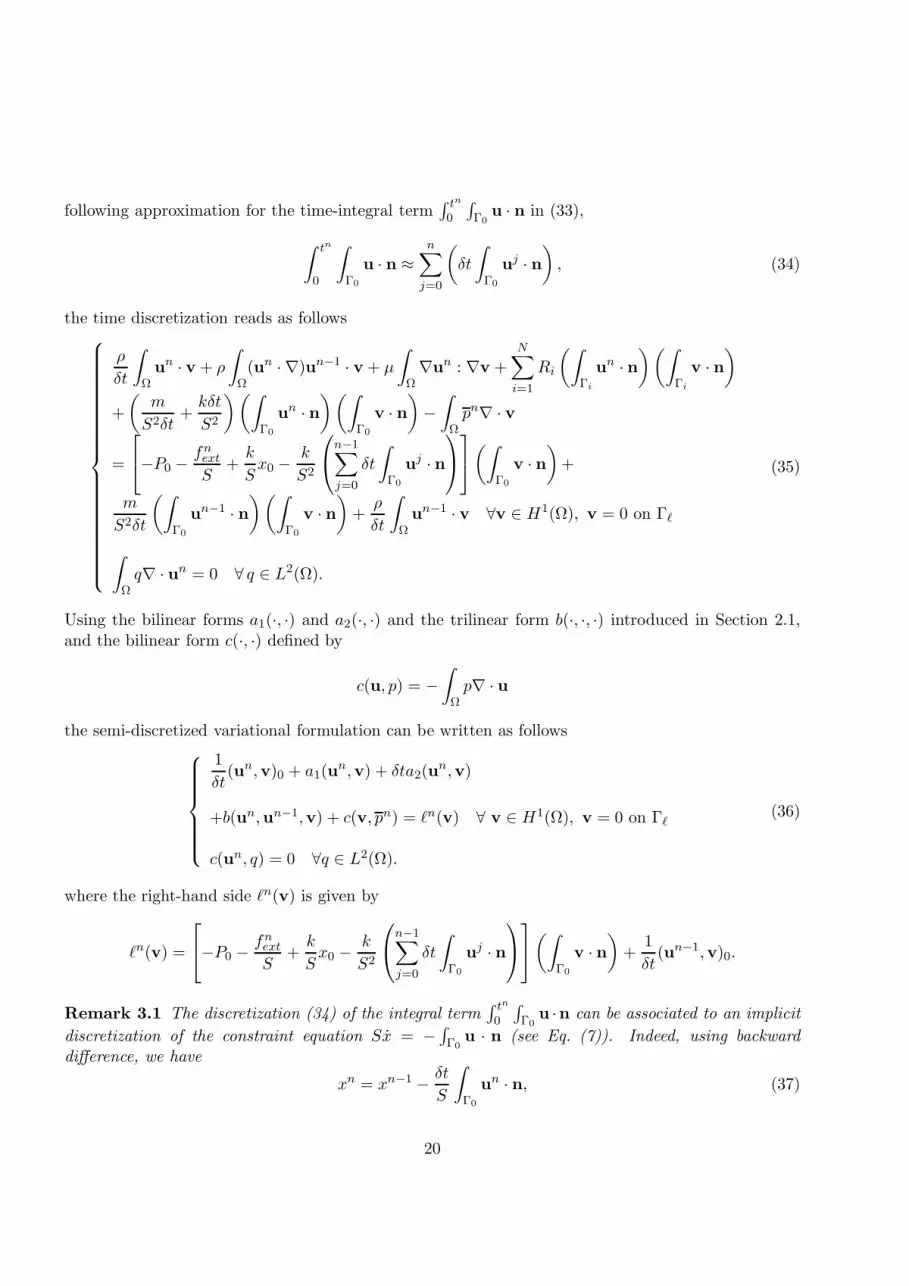
following approximation for the time-integral term∫ tn

0

∫

Γ0u · n in (33),

∫ tn

0

∫

Γ0

u · n ≈n∑

j=0

(

δt

∫

Γ0

uj · n)

, (34)

the time discretization reads as follows

ρ

δt

∫

Ωun · v + ρ

∫

Ω(un · ∇)un−1 · v + µ

∫

Ω∇un : ∇v +

N∑

i=1

Ri

(∫

Γi

un · n)(∫

Γi

v · n)

+

(m

S2δt+

kδt

S2

)(∫

Γ0

un · n)(∫

Γ0

v · n)

−∫

Ωpn∇ · v

=

−P0 −fn

ext

S+

k

Sx0 −

k

S2

n−1∑

j=0

δt

∫

Γ0

uj · n

(∫

Γ0

v · n)

+

m

S2δt

(∫

Γ0

un−1 · n)(∫

Γ0

v · n)

+ρ

δt

∫

Ωun−1 · v ∀v ∈ H1(Ω), v = 0 on Γℓ

∫

Ωq∇ · un = 0 ∀ q ∈ L2(Ω).

(35)

Using the bilinear forms a1(·, ·) and a2(·, ·) and the trilinear form b(·, ·, ·) introduced in Section 2.1,and the bilinear form c(·, ·) defined by

c(u, p) = −∫

Ωp∇ · u

the semi-discretized variational formulation can be written as follows

1

δt(un,v)0 + a1(u

n,v) + δta2(un,v)

+b(un,un−1,v) + c(v, pn) = ℓn(v) ∀ v ∈ H1(Ω), v = 0 on Γℓ

c(un, q) = 0 ∀q ∈ L2(Ω).

(36)

where the right-hand side ℓn(v) is given by

ℓn(v) =

−P0 −fn

ext

S+

k

Sx0 −

k

S2

n−1∑

j=0

δt

∫

Γ0

uj · n

(∫

Γ0

v · n)

+1

δt(un−1,v)0.

Remark 3.1 The discretization (34) of the integral term∫ tn

0

∫

Γ0u ·n can be associated to an implicit

discretization of the constraint equation Sx = −∫

Γ0u · n (see Eq. (7)). Indeed, using backward

difference, we have

xn = xn−1 − δt

S

∫

Γ0

un · n, (37)

20

so, by downward recursion to initial position x0,

xn = x0 − δt

S

n∑

j=0

∫

Γ0

uj · n, (38)

so that the mass position at time tn is implicitly calculated and can be determined using (37) or (38)after the resolution of the modified Navier–Stokes system (36).

In the same way, part of the right-hand side of the mixed variational formulation (36) correspondsto the following time discretization of the mass-spring differential equation (4)-(5), coupled with theconstraint equation (6) or (7), using an implicit central difference scheme

Pna =

1

S

(

mxn − 2xn−1 + xn−2

δt2+ kxn − fn

ext

)

(39)

and using (37) and (38),

Pna =

1

S

−m

δt

(∫

Γ0

un · n−∫

Γ0

un−1 · n)

+ k

x0 − δt

S

n∑

j=0

∫

Γ0

uj · n

− fnext

.

Remark 3.2 Note that another –equivalent– discretization strategy consists in consider the variationalformulation obtained by using (8) as the starting system, instead of the system (10). In this approach,the surface integral terms on Γ0 would be written in terms of the sum of surface integrals on Γi, thatis in the semi-discretized variational formulation we would deal with a quadratic term of the form

(m

S2δt+

kδt

S2

)( N∑

i=1

∫

Γi

un · n)(

N∑

i=1

∫

Γi

v · n)

.

Hence, in a finite element framework, this would imply that all the degrees of freedom belonging tothe outlet boundaries Γi, i = 1, . . . , N , would be coupled. The two formulations are equivalent as faras discrete solutions are concerned. Yet, the resulting matrices differ in the way degrees of freedomare coupled, and numerical tests suggest that the system resulting from formulation (35) is betterconditionned.

3.2 Space discretization

The solver uses a P1/P1 stabilized finite element method (FEM) for the space discretization of Navier–Stokes systems. The linear systems obtained are then solved using a preconditioned GMRES iterativeroutine.

As seen before, the dissipative conditions coming from the resistance and the mass-spring time–discretization modify the bilinear forms in the variational formulation and, therefore, they wouldmodify the FEM matrix associated to the velocity degrees of freedom. However, from the variationalformulation we see that these modifications can be seen as an additive perturbation of the originalFEM matrix,

A = AΩ + Ares. (40)

21

where AΩ stands for the standard FEM matrix over Ω, and Ares stands for the matrix associated toresistances.

The matrix Ares is not assembled : matrix–vector products involving Ares are performed as tensoroperations based on a vector whose entries depend on

∫

Γjφi · n (where φi is a FEM velocity basis

function), the resistance values Rj, j = 1, . . . , N , and the modified resistance value R0 = R0 +S−2(mδt−1 + kδt) (for the entries associated to nodes on Γ0).

Remark 3.3 When considering only the Navier–Stokes system with natural dissipative boundary con-ditions (3) then one could impose these conditions explicitly. In this case the FEM matrice of thesystem is AΩ. Nervetheless for large resistance value Ri this may be unstable, as suggested by thesufficient existence condition that one will obtain by omitting the resistive part in the definition of thebilinear form of the system (see Remark 2.13).

Remark 3.4 If the second variational formulation were used (see Remark 3.2), then the matrixproduct Aresx would be more complicated, since all the outlets’ degrees of freedom would be cou-pled. Moreover each entry associated to an outlet’s degree of freedom would depend on the coefficientS−2(mδt−1 + kδt) coming from the spring-mass system time discretization.

Note on the preconditioner

As the preconditioner for the modified linear system we use the incomplete LU (ILU) preconditionerassociated to the original FEM matrices which demonstrates to be sufficient for the physiological nu-merical tests we performed. Nevertheless for large values of the subtrees resistance this preconditionermay not be appropriated.

4 Numerical results

In this section we present 3D numerical results of the coupled Navier–Stokes/mass-spring system,performed with an academic code developed at INRIA-Rocquencourt which has implemented thenatural dissipative boundary conditions in an implicit way (see [26]). We illustrate how this approachmakes it possible to investigate the effect of a modification of some resistances in the condensed(distal) part onto the overall flow in the upper (proximal) part of the tree. We will also test theeffect of a modification of the spring stiffness. The goal of this section is to illustrate the feasibilityfrom a numerical point of view of the model using a realistic geometry and realistic data. The precisephysiological exploitation of the multiscale system will be the object of a forthcoming paper.

4.1 Methodology, data

We have performed numerical calculations of the coupled Navier–Stokes/mass-spring system in a 3Dreconstructed bronchial tree (until 6th − 7th generation). The tetrahedral meshes (see Fig. 2) wereconstructed using INRIA GHS3D mesh generator [16]. The original 3D surface geometry is the sameused in [14, 13], and it was reconstructed, from CRT medical images, using a marching cube-baseadaptive approach (see [14] for more details) .

22

Mesh size

We use a tetrahedral mesh composed of Nnodes = 31288 nodes, Ntetra = 131562 tetrahedra andNtriang = 33950 surface triangles.

Figure 2: Reconstructed bronchial tree. Cut planes (yellow) after first bifurcation.

Resistance values

The resistance values were estimated using anatomical data from [40], assuming that each outlet Γi isconnected to a dyadic subtree which is assumed to follow a geometric decrease of the pipe sizes, andtherefore a geometric increase of individual pipe resistances. As the outlets correspond to differentgenerations (j0 =4, 5, 6, 7, and 8), the corresponding resistances are computed as partial sums of thetype

R =

17∑

j=j0

rj

2j−j0+1, rj =

128µ

π

ljd4

j

, (41)

where lj and dj stand for the bronchus’ length and diameter, respectively. Note that a dissipativeboundary condition is prescribed at inlet Γ0, to account for the resistance of the upper part of therespiratory tract (nose, pharynx, and larynx). The corresponding resistance value is taken from [4, 25].

23

The table below presents the resistance values (in g · cm−4 ·s−1) for the inlet and for the 58 outlets(the value depends on the generation j0 only).

generation (j0) R

0 1.12E+004 2.24E+005 3.89E+006 6.59E+007 1.10E+018 1.70E+01

Fluid and spring parameters

The fluid is supposed to be air saturated in water vapor, and its dynamic viscosity and density aregiven by

µ = 1.98 × 10−4 g · cm−1 · s−1, ρ = 1.11 × 10−3 g · cm−3

so that the kinematic viscosity is given by ν = µ/ρ = 0.18 cm2 · s−1. For the mass-spring system, wehave used the same values as in [25]:

m = 300 g, S = 100 cm2, k = 3.63 × 103 dyn · cm−1,

4.2 Results

We present the numerical results obtained in the case of normal respiration simulations and in the caseof forced maneuvers simulations. In the case of normal respiration simulations we apply a periodicsmoothed pulse force (of period T = 4 s) with fmax = 1.5 × 105 dyn and fmin = 0. Figure 3 showsthe mass-spring displacement x (in cm) versus time t (in s) and air flow Q (in cm3 · s−1) throughboundary Γ0 versus time t. Note that xmax ≈ 4 cm, therefore the tidal volume VT is approximately

0

1

2

3

4

0 2 4 6 8 10 12-800

-600

-400

-200

0

200

400

600

800

0 2 4 6 8 10 12

Figure 3: Mass-spring displacement x and air flow Q versus time.

equal to 400cm3, since S = 100 cm2, which is the average value for an healthy adult.

24

Figure 4: Isovalues of the velocity vector field norm on cut plane on left first bifurcation, at peakinspiration (t = 0.4s, left), transition (t = 1.6s, middle), peak expiration (t = 1.9s, right)

Figure 5: Isovalues of the velocity modulus on cut plane on right first bifurcation. at peak inspiration(t = 0.4, left), transition (t = 1.6, middle), peak expiration (t = 1.9, right)

Figures 4 and 5 show the isovalues of the velocity vector field norm, interpolated on two cut planesimmediately after the first bifucation (see Fig. 2), at peak inspiration (t = 0.4s), transition (t = 1.6s)and peak expiration (t = 1.9s).

We can observe that, in our experiments, the velocity profiles in these sections differ from inspira-tion and expiration and that during transition, as expected, more complex velocity profiles are formedin the upper airways. At the peak of inspiration we obtain a typical M-shape after the first bifurcation(see [13] where steady state simulations and experiments are performed on the same geometry).

Note that our numerical simulations are not able to capture the possible turbulent patterns of theflow since it will require a much more finer mesh and a parallel solver to perform DNS (Direct Navier-Stokes) simulations. Note moreover that in [9], [11], [14] the authors assume that the flow is laminar,at least for the respiration at rest. It seems to be due to the oscilatory character of the respirationwhich prevents the development of the turbulence patterns. Nevertheless, the geometries used toperform the simulations in the previous papers (as in the present work) go from the trachea up tofew generations of the bronchial tree. It is worth noticing that a recent study [23], where steady stateDNS simulations, with prescribed boundary conditions at the outlets and at the inlet, are performed,shows that for a geometry going from the mouth up to the to the 6th generation turbulence patternsappear. Whereas considering a geometry going from the trachea to the 6th generation, for a steadyflow, the turbulence is negligible. The model we propose could provide a tool to determine whether ornot turbulent patterns appear in a pulsatile regime, by performing DNS simulation in a full geometryincluding the mouth-larynx system, with physically relevant driving forces, and free inlet boundaryconditions.

25

Parametric studies

In Figure 6 we compare the pressure field of the previous simulation at peak expiration with the caseof a partially obstructed bronchial tree at the same time. The obstruction is obtained by increasingsome resistance values (in this experiment, the resistances associated to the encircled outlets in Fig. 6right). It shows that the qualitative behaviour of the flow is modified just by increasing few outletresistances. Note that during an asthma crisis this is roughly what happens: the resistances of smallairways in the distal part increase due to the inflammation process.

Figure 6: Pressure field in the standard (left) and obstructed (right) situations

Next we provide some experiments for forced respiration. In order to simulate the clinical experi-ence of a normal subject performing forced maneuvers, we use a nonlinear constant k = k(x) as in [25].Indeed, in this case one needs to take into account the fact that the motion of the lung parenchymais limited by the chest wall in order to capture the limitation of the inhaled volume. More precisely:

k(x) = k0 +

(fmin/xmin − k0)x/xmin, if x < 0(fmax/xmax − k0)x/xmax, if x ≥ 0.

with fmin = −11 × 105 dyn and fmax = 13 × 105 dyn and k0 = 3.63 × 103dyn · cm−1. The externalforce belongs to the following intervals:

fext ∈ [−1.0 × 105, 2.5 × 105] in dyn (normal), fext ∈ [−11 × 105, 13 × 105] in dyn (forced).

The phase portrait (instantaneous flux vs. inhaled volume) is the curve obtained by spirometry,which provides pneumologists with information on the pathologies a patient may suffer. Figure 7presents such a curve obtained by measurements, and Figure 8 the numerical results obtained afteran appropriate tuning of the forcing term fext.

The model allows to investigate the influence of pertubations on the phase diagram, and thus toquantify the observability of different parameters with respect to this phase diagram. In this spirit,we can compute and compare phase diagrams obtained for different values of k (see Fig. 9), and fordifferent values of the distal resistance (Fig. 10). By these simulations we would like to emphasize

26

that the coupled model we propose may be useful to reproduce some pathological features. A precisephysiological exploration, in collaboration with lung specialists, still needs to be done.

3 2 1 0 −1 −2 −3 6

4

2

0

−2

−4

−6

−8

−10

−12

(I)

(E)

Measured volume (L)

Flo

w (

L/s)

Figure 7: Measured Displacement (in cm)- Flow (in cm3 · s−1) diagram.

5 Conclusions

The proposed well–posed multiscale model enables to describe the air flow behavior in the proximalpart of the bronchial tree taking into account the parenchyma and diaphram motions. We have studiedthe numerical feasibility of the model on a 3D real geometry with realistic data. Note that in thiswhole coupled model we have only few parameters to fit: m, k, S, fext and the resistances Ri. Inparticular by modifying k and Ri one can expect to reproduce some aspects of pathological behaviorssuch as asthma (increase of the resistances) or emphysema (decrease of k) by fitting to phase portraitand look, then, at the modifications induced for the 3D flow. Nevertheless, we may have to modifythe spring model to capture some of the non linear effects of the phenomenon and the physiologicalexploitation of this multiscale system will be the object of a forthcoming paper.

A Hardy inequality in a quarter space

We establish here a special Hardy inequality which is needed in the proof of Prop. 2.8. We considerthe quarter space

Ω =x = (x1, x2, x3) = (x′, x3) ∈ R

3 , x1 ≥ 0 , x2 ≥ 0

.

27

-12

-10

-8

-6

-4

-2

0

2

4

6-3-2-1 0 1 2 3

Flo

w (

L/s)

Volume (L)

Figure 8: Displacement (in cm)- Flow (in cm3 · s−1) diagram.

For any u in L2(R3), we denote by u its Fourier transform, we set |u|2s =∫

R3 |ξ|2s |u(ξ)|2 dξ and we

denote by Hs(R3) the set of functions for which this quantity is bounded. The homogeneous Sobolevspace Hs over Ω is defined as

Hs(Ω) =

u|Ω , u ∈ Hs(R3)

,

and it is endowed with the following semi-norm

|u|Hs(Ω) = infu|Ω=u

|u|s .

Finally, for v defined over Rd, sufficiently regular, we define |D|η v by

(|D|η v)(x) = (2π)−d

∫

Rd

eix·ξ |ξ|η v(ξ) dξ.

Proposition A.1 Let δ ∈ (0, 1/2) be given. There exists a constant C > 0 such that, for any regularfunction u which vanishes on [x2 = 0] ∩ ∂Ω,

|u|H2−δ(Ω) ≤ C∥∥∥

∣∣x′∣∣δ D2u

∥∥∥

L2(Ω),

where D2u is the Hessian matrix of u, and |x′| = (x21 + x2

2)1/2 is the distance to the x3-axis.

28

-12

-10

-8

-6

-4

-2

0

2

4

6-3-2-1 0 1 2 3

Flo

w (

L/s)

Volume (L)

reference k_0100% increased k_0

Figure 9: Phase diagram for different values of k0

Proof: The proof decomposes into 4 steps.a) Fractional Hardy inequality in R

2

The standard Hardy inequality (which involves u and its gradient) is also valid in the case fractionalderivatives: ∥

∥∥∥∥

u

|x′|δ

∥∥∥∥∥

L2(R2)

≤=∥∥∥|D|δ u

∥∥∥

L2(R2), (42)

for any function u defined over R2, and δ ∈ (0, 1). The proof is given in [37, 2].

b) Hardy inequality in R3, cylindrical setting

We prove here that the previous inequality extends to R3, with a weight equal to the distance |x′| to

the x3-axis. Let u denote a regular function defined over R3. With obvious notations, one has

∫

R3

|u|2

|x′|2δ=

∫

R

(∫

R2

|u|2

|x′|2δdx′

)

dx3 .

∫

R

∥∥∥|D|δ u

∥∥∥

2

L2([x3=s])ds =

∥∥∥|D|δ u

∥∥∥

2

L2(R3)(43)

c) Hardy inequality with a weight in the right-hand sideLet u and v be regular functions over R

3. One has

(

|D|2−δ u, v)

L2(R3)=

(

∣∣x′∣∣δ |D|2 u,

1

|x′|δ|D|−δ v

)

≤∥∥∥

∣∣x′∣∣δ |D|2 u

∥∥∥

L2(R3)‖v‖L2(R3)

29

-12

-10

-8

-6

-4

-2

0

2

4

6-3-2-1 0 1 2 3

Flo

w (

L/s)

Volume (L)

reference R_i100% increased R_i

Figure 10: Phase diagram for different values of the distal resistances

(thanks to (43), which we apply to |D|−δ v). As a consequence, one has

|u|H2−δ(R3) .∥∥∥

∣∣x′∣∣δ D2u

∥∥∥

L2(R3). (44)

d) Hardy inequality in the quarter-spaceLet u be a regular function defined over the quarter space Ω = [x1 ≥ 0, x2 ≥ 0]. We assume that uvanishes on [x2 = 0]. We extend u over R

3 in two steps: firstly, we define u1 over [x1 ≥ 0] as follows:

u1(x1, x2, x3) =

∣∣∣∣∣

u(x1, x2, x3) if x2 ≥ 0

−u(x1,−x2, x3) if x2 ≤ 0

this extension preserves the L2 norm of |x′|δ D2u (up to a factor 2). We extend now u1 over R byfollowing a Babitch process:

u2(x1, x2, x3) =

∣∣∣∣∣

u1(x1, x2, x3) if x1 ≥ 0

3u1(−x1, x2, x3) − 2u1(−2x1, x2, x3) if x1 ≤ 0

This extension preserves again the L2 norm of |x′|δ D2u1 (up to a multiplicative constant). Inequal-ity (44) can be applied to u2, which ends the proof.

Acknowledgements The authors would like to acknowledge the support of ACINIM project LeP-oumonVousDisJe, and to thank M. Dauge for fruitful discussions, M. Grasseau for his technical helpwith the mesh, and P. Gerard for his help in proving Proposition A.1.

30

References

[1] V. Antonaglia, L. Torelli, W.A. Zin and A. Gullo, Effects of viscoelasticity on volume distributionin a two-comportmental model of normal and sick lungs, Physiol. Meas. 26 (2005), 13–28.

[2] H. Bahouri, J.-Y. Chemin and I. Gallagher, Ingalites de Hardy precisees, C. R. Math. Acad. Sci.Paris 341 (2005), no. 2, 89–92.

[3] R. Begin, A.D. Renzetti Jr., A.H. Bigler and S. Watanabe, Flow and age dependence of airwayclosure and dynamic compliance, J. Appl. Physiol. 38 (1975), no 2, 199–207.

[4] A. Ben-Tal, Simplified models for gas exchange in the human lungs, J. Theor. Biol. 238 (2006),474–495.

[5] W. Benish, P. Harper, J. Ward and J. Popovich, Jr., A mathematical model of lung static pressure-volume relationships: comparison of clinically derived parameters of elasticity, Henry Ford Hosp.Med. J. 36 (1988), no 1, 44–47.

[6] H. Brezis, Analyse Fonctionnelle, Theorie et applications, Ed. Dunod, 1994.

[7] G.P.S. Crooke, J.D. Head and J.J. Marini, A general two-compartment model for mechanicalventilation, Math. Comput. Modelling 24 (1996), no. 7, 1–18.

[8] Y.H. Chang and C.P. Yu, A model of ventilation distribution in the human lung, Aer. Sci. Tech.30 (1999), 309–319.

[9] C. Croce, R. Fodil, M. Durand, G. Sbirlea-Apiou, G. Caillibotte, J.-F. Papon, J.-R. Blondeau,A. Coste, D. Isabey and B. Louis, In vitro experiments and numerical simulations of airflowin realistic nasal airway geometry Annals of biomedical engineering, (2006) Vol. 34, no6, pp.997–1007.

[10] M. Dauge, Elliptic boundary value problems on corner domains, Smoothness and asymptotics ofsolutions, Lecture Notes in Mathematics, 1341. Springer-Verlag, Berlin, 1988.

[11] J.W. De Backer, W.G. Vos, A. Devolder, S.L. Verhulst, P. Germonpre, F.L. Wuyts, P.M. Parizeland W. De Backer Computational fluid dynamics can detect changes in airway resistance inasthmatics after acute bronchodilation, Journal of Biomechanics 41 (2008) 106–113.

[12] L. de Rochefort, X. Maıtre, R. Fodil, L. Vial, B. Louis, D. Isabey, C. Croce, L. Darrasse,G. Sbirlea-Apiou, G. Caillibotte, J. Bittoun and E. Durand, Phase contrast velocimetry withhyperpolarized helium-3 for in vitro and in vivo characterization of airflow Magn Reson Med2006;55:1318-1325.

[13] L. de Rochefort, L. Vial, R. Fodil, X. Matre, B. Louis, D. Isabey, G. Caillibotte, M. Thiriet,J. Bittoun, E. Durand and G. Sbirlea-Apiou, In vitro validation of computational fluid dynamicsimulation in human proximal airways with hyperpolarized 3He magnetic resonance phase-contrastvelocimetry, J. Appl Physiol, 102, pp. 2012-2023, 2007.

31

[14] C. Fetita, S. Mancini, D. Perchet, F. Preteux, M. Thiriet and L. Vial, An image based compu-tational model of oscillatory flow in the proximal part of tracheobronchial trees, Comput. Meth.Biomech. Biomed. Eng., 8 (2005), pp. 27–293.

[15] L. Formaggia, F. Nobile, A. Quarteroni and A. Veneziani, Multiscale modelling of the circulatorysystem: A preliminary analysis, Comput. Visualization Sci. 2 (2/3) (1999) 7583.

[16] GHS3D, tetrahedal mesh generator, INRIA-Simulog, 2005http://www-c.inria.fr/gamma/ghs3d

[17] V. Girault, P.-A. Raviart, Finite Element Approximation of the Navier-Stokes Equations, LectureNotes in Mathematics, Vol. 749 Springer Verlag, Berlin, 1979.

[18] C. Grandmont, Y. Maday and B. Maury, A multiscale / multimodel approach of the respirationtree, Proceedings of the International Conference “New Trends in Continuum Mechanics” 8-12September 2003, Constantza, Romania Theta Foundation Publications, Bucharest, 2005.

[19] C. Grandmont, B. Maury and N. Meunier, A viscoelastic model with non-local damping applicationto the human lungs, Math. Mod. Numer. Anal. 40 (2006), no 1, 201–224.

[20] C. Grandmont, B. Maury and A. Soualah, Multiscale modelling of the respiratory tract: a theo-retical framework, ESAIM: PROCEEDINGS, June 2008, Vol. 23, p. 10-29

[21] J. G. Heywood, The Navier-Stokes equations : on the Existence, Regularity and decay of Solution,Indiana Univ. Math. J., 29, pp. 636–681 (1980).

[22] J. G. Heywood, R. Rannacher and S. Turek, Artificial boundaries and flux and pressure conditionsfor the incompressible Navier-Stokes equations, International Journal for Numerical Methods inFluids, 22, pp. 325–352 (1996).

[23] C.-L. Lin, M. H. Tawhai, G. McLennanc and E.A. Hoffman Characteristics of the turbulentlaryngeal jet and its effect on airflow in the human intra-thoracic airways, Respiratory Physiology& Neurobiology, 157, pp. 295–309, (2007).

[24] J. L. Lions, Quelques methodes de resolution des problemes aux limites non lineaires, Dunod,2002.

[25] S. Martin, B. Maury, T. Similowski and C. Straus, Modelling of respiratory system mechanicsinvolving gas exchange in the human lungs, ESAIM: PROCEEDINGS, June 2008, Vol. 23, p.30-47.

[26] B. Maury, N. Meunier, A. Soualah and L. Vial, Outlet Dissipative conditions for air flow inthe bronchial tree, ESAIM Proceedings, september 2005, vol. 14, 115-123, Eric Cances & Jean-Frederic Gerbeau, Editors.

[27] B. Mauroy, M. Filoche, J.S. Andrade Jr. and B. Sapoval, Interplay between flow distribution andgeometry in an airway tree, Phys. Rev. Lett. 90, 14 (2003).

32

[28] V. Maz’ya and J. Rossmann, Point estimates for Green’s matrix to boundary value problems forsecond order elliptic systems in a polyhedral cone ZAMM Z. Angew. Math. Mech. 82 (2002), no.5, 291–316.

[29] V. Maz’ya and J. Rossmann, Lp estimates of solutions to mixed boundary value problems for theStokes system in polyhedral domains, Math. Nachr. 280 (2007), no. 7, 751–793.

[30] M.S. Olufsen, Structured tree outflow condition for blood flow in larger systemic arteries, Am. J.Physiol. 276 (1999) 257–H268.

[31] Mathematical Models in Human Physiology, J.T. Ottesen, M.S. Olufsen, J.K. Larsen (editors),SIAM, Philadelphia, 2004.

[32] M. Orlt and A.-M. Sandig, Regularity of viscous Navier-Stokes flows in nonsmooth domains.Boundary value problems and integral equations in nonsmooth domains (Luminy, 1993), 185–201, Lecture Notes in Pure and Appl. Math., 167, Dekker, New York, 1995.

[33] A. Quarteroni and A. Veneziani, Analysis of a Geometrical Multiscale Model Based on the Cou-pling of ODEs and PDEs for Blood Flow Simulations, Multiscale Model. Simul., Vol. 1, No. 2,173-195, 2003.

[34] A. Quarteroni, S. Ragni and A. Veneziani, Coupling between lumped and distributed models forblood flow problems, Comput. Visualization Sci. 4 (2) (2001) 111-124.

[35] J.R. Rodarte and K. Rehder, Dynamic of respiration, In: Handbook of physiology: the respiratorysystem, A.P. Fishman, P.T. Macklem, J. Mead and S.R. Geiger (editors), Americal PhysiologicalSociety, 131–144, 1986.

[36] T. Similowski and J.H.T. Bates, Two-compartment modelling of respiratory system mechanics atlow frequencies: gas redistribution or tissue rheology?, Eur. Respir. J. 4 (1991), 353–358.

[37] F. Vigneron Espaces de Sobolev d’ordre variable : traces, eclatement, inegalite de Hardy,Seminaire Equations aux derivees partielles (Polytechnique) (2006-2007), Exp. No. 17.

[38] I. E. Vignon-Clementel, C. A. Figueroa, K. E. Jansen and C. A. Taylor, Outflow boundary con-ditions for three-dimensional finite element modelling of blood and pressure in arteries, Comput.Methods Appl. Mech. Engrg., 195, 3776-3796 , 2006.

[39] J.G. Venegas, R.S. Harris and B.A. Simon, A comprehensive equation for the pulmonary pressure-volume curve, J. Appl. Physiol. 81 (1998), no 1, 389–395.

[40] E.R. Weibel, Morphometry of the human lung, Springer Verlag and Academic Press, Berlin, NewYork, 151 pp., 1963.

[41] J.B. West, J.B. Respiratory Physiology - The Essentials, Baltimore: Williams & Wilkins, 1974.

[42] The lung: scientific foundations, R.G. Crystal, J.B. West, E.R. Weibel and P.J. Barnes (editors),2 Vol., 2nd Edition, Lippincott-Raven Press, Philadelphia, 1997.

33