computed tomography - International Nuclear Information ...
151
INIS-mf —11 OO6 COMPUTED TOMOGRAPHY OF THE PETROUS BONE IN OTOSCLEROSIS AND MENIERE'S DISEASE J.A.M.DEGROOT
-
Upload
khangminh22 -
Category
Documents
-
view
0 -
download
0
Transcript of computed tomography - International Nuclear Information ...
INIS-mf — 1 1 O O 6
COMPUTED TOMOGRAPHY
OF THE
PETROUS BONE
IN
OTOSCLEROSIS
AND
MENIERE'S DISEASE
J.A.M.DEGROOT
' '. i. i
./„.. COMPUTED TOMOGRAPHY
OF
THE PETROUS BONE
IN
OTOSCLEROSIS
AND
MENIERE'S DISEASE

Cover design: Rene Smoorenburg
DRUKKERIJ ELINKWIJK BV - UTRECHT

RUKSUNIVERSITEIT UTRECHT
COMPUTED TOMOGRAPHY OF THE PETROUS BONE
IN OTOSCLEROSIS AND MENIERE'S DISEASE
Computertomografie van het rotsbeen bij otoscleroseen bij de ziekte van Meniere
(Met een samenvatting in het Nederlands)
PROEFSCHRIFT
ter verkrijging van de graad van doctor in de geneeskundeaan de Rijksuniversiteit te Utrecht,
op gezag van de rector magnificus Prof.Dr. J.A. van Ginkel,volgens besluit van het college van dekanen
in het openbaar te verdedigenop dinsdag 14 april des namiddags te 4.15 uur
in het hoofdgebouw der universiteit
door
Johan Antonius Maria de Groot
geboren te Utrecht

Promotores: Prof. dr. E.H. HuizingProf. dr. P.F.G.M. van Waes

Aan CorrieHarryTrudy

ACKNOWLEDGEMENTS
This dissertation was produced in the Departments of Otorhinolaryngology and of Radiologyof the Utrecht University Hospital, Utrecht, the Netherlands.
The author wishes to thank Prof. dr. Egbert H. Huizing (Head of the Department ofOtorhinolaryngology) who has spent so much time in supervising this work, and Prof. dr.Paul F.G.M. van Waes (Department of Radiology) for his support and enthusiasm. Manythanks are due to Mr. Frans W. Zonneveld M.Sc. (Philips Medical Systems), whose scientificand technical contribution has been essentially for this study, to Dr. Henk Damsma(Department of Radiology) for his evaluation of the CT scans and to Dr. Jan E. Veldman(Department of Otorhinolaryngology) for his valuable corrections and suggestions.
He would like to thank Prof. dr. A.C. Kiinkhamer (Head of the Department of Radiology),Prof. dr. S.A. Duursma (Head of the Department of Internal Medicine, bone metabolism),Prof. dr. W.J. van Doorenmaalen (Head of the Laboratory of Anatomy) and Prof. dr. P.Bretlau (Head of the Department of Otorhinolaryngology of the University of Copenhagen)for their suggestions and scientific judgement.
Many thanks are also due to Mr. Marcel Metselaar for his help in the realization of thephotographical part, Dr. Frank Besamusca for his initial and Mrs. Gayle Johnson for her finallistinguic corrections and to Dr. Kobus Dijkhorst for his support in matters of soft- andhardware.
Finally, the author is very grateful for the moral support of all who have followed theproceedings of this work with interest.
Utrecht, April 1987John de Groot
CONTENTS
PART I Computed Tomography of the petrous bone 1
PART II CT investigation of the cochlear capsule in otosclerosis 33
PART III CT investigation of the vestibular aqueduct in Meniere's disease 95
Summary in Dutch - Samenvatting in het Nederlands 137
Curriculum Vitae 143

GENERAL INTRODUCTION
In this study the pathology of the cochlear capsule in otosclerosis and of the vestibularaqueduct in Meniere's disease was investigated by means of high-resolution CT scanning.Computed Tomography (CT) can be considered as the most important improvement in thearea of X-ray diagnostics during the last twenty years. Technical developments have resultedinto an increase in spatial resolution. The 'high-resolution' scanner of the third generationfacilitates the visualization of the more delicate structures in the temporal bone.
Previous studies on otosclerosis and Meniere's disease (by means of classicalpolytomography) have presented a more or less confusing picture. In this study we tried tofind out if CT scanning of the temporal bone can clarify some of the questions raised bypolytomographical studies.
In order to analyze these problems, this study is divided into three parts:
PART I : Normal radiographical 3natomy of the temporal bone as examined by CTPART II : CT investigation of the cochlear capsule of patients with otosclerosisPART III : CT investigation of the vestibular aqueduct in patients with Meniere's disease.
In PART I a brief description is given of the high resolution CT scanner used in this study.Some principles of computed tomography are explained in relation to the analysis ofanatomical and pathological details of the temporal bone. The specific otoradiological planesare described, in particular those planes used in our patient study. The normal anatomy of thetemporal bone is presented in six otoradiological planes. In each plane seven consecutive CTslices are given.
In PART II a short introduction is presented to the clinical aspects and the histopathologyof otosclerosis, followed by a review of the literature.In our own study we have tried to find an answer to the next main questions:
- In which otoradiological planes can the cochlear capsule be optimally visualized with CT?- What is the normal density of the labyrinthine capsule? Is it dependent on age?- Is it possible to detect foci of otospongiosis and otosclerosis by means of CT?- Is there a correlation between the degree of demineralizaiion in a focus and the degree of boneconduction hearing loss?- Is a correlation present between the location of density loss in the cochlear capsule and themagnitude of inner ear impairment for the place corresponding frequency?
This study concerns a CT investigation of the labyrinthine capsule in 35 normal ears and 134

ears of 84 patients with surgically confirmed otosclerosis. CT scans are judged by the nakedeye and by densitometry. The maximum and minimum density of the cochlear capsule ismeasured both in normal and patients' ears. Bone density is also measured at six predefinedpoints within the cochlear capsule. The results of densitometry are correlated with the innerear impairment as measured by bone conduction audiometry.
In PART III the clinical aspects of Meniere's disease are summarized includinghistopathology, anatomy and pathophysiology of the endolymphatic duct within thevestibular aqueduct. Earlier research on polytomographical visualization of the vestibularaqueduct is reviewed.The purpose of this part of the study is to investigate, by means of CT, visibility and lengthof the vestibular aqueduct and to compare our results with the inconsistent (and oftencontroversial) results in the literature. Therefore we have defined strict inclusion and exclusioncriteria in diagnosing Meniere's disease. The following questions are studied:
- Which otoradiological planes are optimal for visualization of the vestibular aqueduct?- Is it possible to find a qualitative method to establish the dimensions of this aqueduct?- Does the visibility and length of the vestibular aqueduct in affected ears of patients withMeniere's disease differ from that in normal ears?- Is there a difference in visibility and length of the vestibular aqueduct between affected andnon-affected ears in patients with unilateral Meniere's disease?- Do the dimensions of the aqueduct correlate with age, duration of the disease or degree ofhearing loss?
In 55 patients with unilateral or bilateral Meniere's disease (104 ears) the vestibular aqueductis investigated by CT. A visibility scale for classification of the vestibular aqueduct isdeveloped and the results, obtained in affected and non-affected ears of patients with Meniere'sdisease, are presented and compared with the CT findings in 50 normal ears. The samecomparisons between Meniere's ears and control ears are made as to the length of thevestibular aqueduct. The results are compared with those from previous polytomographic anddissection studies.

IPAOTK
COMPUTED TOMOGRAPHY
OF
THE TEMPORAL BONE

I. CT of the temporal bone
CONTENTS OF PART I
1. INTRODUCTION 3
1. Some principles of computed tomographyin relation to the analysis of temporal bone details 31. Hounsfield Unit scale 32. Image reconstruction 43. Partial volume averaging 54. Slice thickness 85. Geometrical enlargement 8
2. The Philips Tomoscan 310/350 8
2. OTORADIOLOGICAL PLANES 10
1. Transverse plane (Hirtz) 102. Sagittal plane 133. Coronal plane 134. Axio-petrosal plane (Poschl) 145. Semi-axial plane (Guillen) 146. Semi-longitudinal plane (Zonneveld) 14
3. CT ATLAS 15
Legends 16Visibility matrix 17
1. Transverse plane (Hirtz) 182. Sagittal plane 203. Coronal plane 224. Axio-petrosal plane (Poschl) 245. Semi-axial plane (Guillen) , 266. Semi-longitudinal plane (Zonneveld) 28
4. REFERENCES 30

I. CT of the temporal bone - Introduction
INTRODUCTION
During the last ten years the technology of computed tomography has developed rapidly.Since details smaller than 1 mm can be visualized, CT has been applied more and more toexamine the temporal bone (Hanafee et al, 1979; De Smedt et al, 1980; Shaffer et al, 1980;Littleton et al, 1981; Zonneveld et al, 1981; Rettinger et al, 1981; Zonneveld & Damsma,1982; Valvassori etal, 1982; Swartz, 1983; Zonneveld, 1983). The term 'high resolution' hasto be considered as a relative qualification. At this moment it means that details of about 0.5mm can be visualized (Zonneveld, 1985).
The so called 'third generation' scanner was introduced in 1974 as a brain scanner. It was anentirely new type as compared to the first and second generation scanners. The number ofdetectors was increased and varies from 300 to 700. Therefore the fan angle is widened so thatit can incorporate the whole body cross section. A translating motion (as was necessary informer generations) is no longer needed. These rotate-only scanners work much faster thansecond generation scanners. As a consequence of continuous data aquisition the influence ofthe patient's motion artifacts is much smaller.
SOME PRINCIPLES OF COMPUTED TOMOGRAPHYin relation to the analysis of temporal bone details.
1. Hounsfield Unit Scale
The local attenuation characteristic of tissue for X-rays is the product of a number ofinteracting processes between X-rays and matter such as photoelectric absorption andCompton scatter. X-ray tubes produce radiation in a spectrum of wavelengths. Therefore thetotal transmitted energy is composed of a number of different energies. The attenuationproperty of tissue (the linear attenuation coefficient p.) is a complex function that differs invalue as the energy of radiation is changed.
The following formula describes the attenuation of a monoenergetic X-ray that passes througha sheet of material: I = I o e ^ d (fig. 1.1).
I is the remaining (attenuated) intensity,d is the thickness of the material.|i is the linear attenuation coefficientIo is the initial X-ray intensity.

I. CT of the temporal bone - Introduction
/
•
/
I = I 0 . e
Fig. 1.1. Remaining X-ray intensity (I) of an X-ray with initial intensity (Io) after passagethrough a piece of material with thickness d and a linear attenuation coefficient (i.
The linear attenuation coefficient \i decreases with increasing energy (i.e.: ji is larger for lowerenergies and smaller for higher energies). This results in a loss of the lower energies from theradiation spectrum as it passes through a volume of tissue. The higher energies remain andthe effective \i of the tissue decreases. This effect is called "beam hardening'.
Generally the \i of soft tissue is in the range of the |X of water. The (i of muscle tissue isabout 5% higher and the [i of fat about 10% lower than that of water. Since it is awkward todeal with |X all the time, Hounsfield has defined a new scale for the linear attenuationcoefficient. The unit of this scale is the H (Hounsfield). He defined the CT number of water as0 H and that of air as -1000 H. Subsequently every structure with a density higher than waterwill have a CT number higher than 0.
2. Image reconstruction
Slice thickness in modern CT scanners ranges from 1 to 12 mm. Three-dimensional data areobtained by scanning an object in contiguous slices in a single plane. From these data,images can be reconstructed in any desired direction through the object (multiplanarreconstruction). Alternatively scans can also be made directly in other planes by the use ofdifferent patient positions.
Voxels and pixelsA CT image is composed from a number of picture elements (pixels). The attenuationcoefficient JJ, has to be calculated for each pixel from measurements through that pixel in alldifferent directions in a slice. Usually there are 256 grey levels between black and white. Withspecial 'window techniques' it is possible to translate a small portion of the Hounsfield scale(CT-number scale) into the grey level range (grey scale). All pixels with CT numbers higherthan this portion will be white and lower black. The portion represented by the grey scale iscalled the 'window'.

I. CT of the temporal bone - Introduction
A voxel (volume element) is the volume of material represented by the pixel. Its dimensionsare equal to the pixel-size with a height equal to the slice thickness used (fig. 1.2).
PIKEL
-Slice thickness
UOKELFig.1.2. A voxel (volume element) is the three-dimensional portion of material from which theCT number of the pixel (picture element) is derived. The volume of the voxel is determined bypixel size and slice thickness.
Image reconstruction is the mathematical procedure that has to be applied in order to produce atwo-dimensional distribution of X-ray attenuation values from the profiles of attenuationmeasurements that have been performed in a limited number of directions. Convolution andFourier based algorithms are used in commercially available CT systems
3. Partial volume averaging
Each pixel has a CT number (Hounsfield unit) that is calculated from the attenuationcoefficient of a three-dimensional volume of tissue (voxel). The cubic capacity of this volumedepends on the pixel size and the applied slice-thickness. If a detail is smaller than the slicethickness, each voxel that represents the detail will contain also part of the surroundingtissue. The resulting attenuation coefficient of such a voxel and consequently the CT numberof its pixel depend on the relative quantities of different tissues within the voxel. Values willbe somewhere between those of the detail and those of the surrounding tissue. This results ina contrast reduction in the image between the detail and the surrounding tissue (blurring).
The same effect is responsible for the blurring of boundaries between different tissues if theseboundaries are not exactly perpendicular to the slice. The effect increases with the slicethickness used and with the obliquity of the detail towards the slice direction. In fig. 1.3 anexample is given of this effect. A structure crosses the slice with a thickness h obliquely.Some voxels contain different shares of this structure resulting in different CT numbers of thecorresponding pixels. After translation to grey levels a blurring effect will be visible on theimage (Zonneveld and Vijverberg, 1984).

I. CT of the temporal bone - Introduction
Fig.1.3. A structure (grey) obliquely intersects a number of voxels within a slice with athickness h (upper figure). A blurring effect will be present in the corresponding pixels (lowerfigure).
ArtifactsThe conversion of the ratio of the radiation intensities (Io/I) to the attenuation values isnon-linear as a logarithm is involved. Therefore the partial volume averaging effect canproduce artifacts when the contrast between detail and surrounding tissue is very high (e.gbetween bone and air in the petrous bone). When two of such areas are scanned in the sameslice (as in the transverse plane through both petrous bones), dark bands may be presentconnecting both ears ('petrous bridging' or 'Hounsfield bars') - (Zonneveld & Vijverberg,1984).
The cause of this artifact can be illustrated with two basically different geometries of tissuecombinations within one voxel:
Geometry 1.The boundary between the two different types of tissue is exactly perpendicular to the slice(fig. 1.4). The different ji's (p.j and H2) "iU be averaged and the 'effective p.' equals to0.5^^+0.5(12- Artifacts will not occur as a result of this measurement. After 90 degrees ofscanner rotation, however, a geometry exists which is comparable to geometry 2.

I. CT of the temporal bone - Introduction
AZA1=1
- 0.5 ( M- « + M- ? )e
Fig. 1.4. Geometry 1. Two different types of tissue within one voxel. The boundary between thetissues is perpendicular to the X-ray direction. Io = initial X-ray intensity. I = total attenuatedX-ray intensity.
Geometry 2.The boundary is parallel to the slice (fig. 1.5). There is no 'effective mean n' in this situation.Both tissue types are passed through by half the initial X-ray intensity. The total attenuatedintensity after passing such a voxel will be the sum of these intensities in the two differenttissue-types. This total attenuated intensity (I) is more than that of geometry 1.
0.5
1 = 0.5 I
Fig. 1.5. Geometry 2. Two different types of tissue within one voxel. The boundary between thetissues is parallel to the X-ray direction. Io = initial X-ray intensity. I = total attenuated X-ray
intensity.

I. CT of the temporal bone - Introduction
4. Slice thickness
The slice thickness is the thickness of tissue that contributes to the image. It determines thedegree of the partial volume averaging effect: the thicker the slices, the more blurring of smalldetails.Direct single scans have a better contrast resolution if slice thickness is small. Thicker slices,however, have a better conirast-to-noise ratio (Peyster, 1983; Zonneveld & Vijverberg, 1984).
5. Geometrical enlargement
In 1977 Philips introduced an improved version of the third generation scanner which includedthe principle of geometric enlargement: by changing the distance between the X-ray sourceand the axis of rotation, while the source-detector relation remains fixed, it is possible to scansmaller and larger diameter areas according to the application. This optimizes the use of theavailable number of detectors, resulting in a higher spatial resolution in smaller objects.
THE PHILIPS TOMOSCAN 310/350
The CT scanner we used in our studies is the Philips Tomoscan 310/350, a high resolutionthird generation scanner, with an array of 576 detectors. This scanner had been experimentallyprovided with a table swivel mechanism (fig. 1.6) and special headrests (fig. 1.7) in order tofacilitate direct scanning of the temporal bone in all possible otoradiological planesZonneveld, 1983). As multiplanar reformatting is accompanied by a degradation of the imagequality (Johnson et Korobkin, 1982; Turski et al, 1982), we only used the direct scanningtechnique to depict temporal bone details.
The principle of geometrical enlargement was used in order to obtain a spatial resolution of0.6 mm. The temporal bone was enlarged to an 8 cm square field of view by means of a zoomreconstruction. A matrix of 256^ resulted in a pixel-size of about 0.3 mm.
Other factors contributing to the sharpness of the image were the use of 1200 projectiondirections in a 9.6 second scan time and a Ramp convolution filter. To avoid degradation ofthe image's sharpness by partial volume averaging, a slice thickness of 1.5 mm was used.
For display and photography a window level of 300 H and a window width of 3200 H wereselected. The scans were made at 120 kV and 480 mAs, resulting in a peak skin dose of about8R (80 mGy) - (Zonneveld et al, 1983).

I. CT of the temporal bone - Introduction
Fig.1.6. Table swivel mechanism Fig.1.7. Headrest for direct (sagittal) CT.

I. CT of the temporal bone - Otoradiological planes
OTORADIOLOGICAL PLANES
Many planes of radiologic investigation have been developed and used since the introductionof the classical tomographical techniques (Ziedses des Plantes, 1932). Which plane to usedepends on the lesion one expects and wants to visualize (Valvassori, 1963; Gros et al, 1965;Clausetal, 1980; Vignaud, 1980).
Basically, the application of CT was restricted to the transverse ('axial') and coronal planes.Other planes of interest, as known in classical otoradiology, can be explored since theintroduction of a table swivel mechanism on the Philips Tomoscan 310/350 (Zonneveld et al,1983). This equipment, combined with special headrests, facilitates the examination ofpatients in almost all current otoradiological planes. Only a few of these planes, however,were used for our study and will be briefly described.
Two reference planes through the skull were used to determine the angle of the otoradiologicalplanes (Claus et al, 1980):
^Vertical reference planeThe direction of this plane is clear: median sagittal, dividing the skull into two equal halves.
b. Horizontal reference planeSeveral 'base planes' have been described: the anthropological base plane, the orbito-meatalplane and the nasion-biauricular (N.B.P.) plane (Dulac's classification of anteroposteriorprojections for petrous bone radiography) - (Dulac, 1956). The latter (N.B.P.) was chosen as astarting point in determining the otoradiological planes used in our studies. This plane joinsthe nasion to the superior borders of both external auditory canals and is also known as theN2A plane.
1. The transverse plane (Hirtz)
This plane, well known in classical tomography, has its incident angle perpendicular to thenasion-biauricular plane and parallel to the vertical reference plane (Hirtz, 1922). Therefore theCT images of this plane lie parallel to the nasion-biauricular plane (fig.1.8). They are realaxial or horizontal projections in line with the axis of the skull. To avoid confusion with theaxiopetrosal or 'axial' plane we will use the term transverse plane.
In all f.yaminp.ri patients the transverse plane was made in order to have an adequate startingpoint for other projections. The patient's position in the scanner can be corrected, if necessary,after composing just one CT image. The position of the patient in the transverse plane iscomfortable.
The majority of details in the temporal bone can be imaged in the transverse plane (Russell etal, 1982; Zonneveld et al, 1983). This fact combined with the patient's comfort and thepossibility to compare both petrous bones with one scan makes, this plane ideal for the

I. CT of the temporal bone - Otoradiological planes
baseline study. In general, the examination area extends from the upper border of the superiorsemicircular canal down to the lower part of the basal cochlear turn. Usually one other plane,perpendicular to the transverse plane, is selected to complete the bi-plane examination.Selection of this second plane depends on the pathology and the anatomical details to beimaged.Slice incrementation normally is 1.5 mm. In order to examine the whole temporal bone inthis (transverse) projection, about seven images are needed.
Fig. 1.8. Direction of the the transverse plane (Hirtz) through the skull.This plane lies parallel to the nasion-biauricular reference plane and is used as starting point forother otoradiological planes.
PSCSPN
VA
Fig. 1.9. Direction of the transverse plane (Hirtz) through the right ear.SSC = Superior semicircular canal. LSC = Lateral semicircular canal. PSC = Posteriorsemicircular canal. M = Malleus. I = Incus. S = Stapes. VA = Vestibular aqueduct. SPN =Superficial petrosal nerve. RW = Round window. FN1 = Facial nerve (proximal part). FN3 =Facial nerve (vertical part). GG = Geniculate ganglion.
11

I. CT of the temporal bone - Otoradiological planes
Fig.1.10. Cranial view on the right temporal bone (transverse plane).
A = Antrum. AA = Aditus ad antrum. C = Cochlea. CAR = Carotid artery. CC = Common crus.CP = Cochleariform process. EAC = External auditory canal. ES -• Endolymphatic sac. ET =Eustachian tube. FN1 = Facial nerve (proximal part). FN2 = Facial nerve (horizontal part). FN3= Facial nerve (distal part). GG = Geniculate ganglion. I = Incus. IAC = Internal auditory canal.LSC = Lateral semicircular canal. M = Malleus. MAS = Mastoid. PE = Pyramidal eminence. PSC= Posterior semicircular canal. S = Stapes. SPN = Superficial petrosal nerve. SS = Sigmoidsinus. SSC = Superior semicircular canal. TC = Tympanic cavity. TM = Tympanic membrane.TTM = Tensor tympani muscle. V = Vestibule. VA = Vestibular aqueduct.
The longitudinal axis of the petrous bone has an angle of about 35 degrees from the coronalplane and 125 degrees from the sagittal plane (flg.1.11) although a considerable variationexists (Korach & Vignaud, 1981). Due to this variation, the transverse plane is used as thefirst plane of examination in order to determine major deviations of the angle and to correctfor other planes.
The other otoradiological planes used in our studies are all perpendicular to the transverseplane and will be briefly described in combination with exemples of the most outstandingslices. Assuming that the pyramidal axis has an angle of 35 degrees from the coronal plane,angles between these planes are given in fig. 1.11.
12
I. CT of the temporal bone - Otoradiological planes
AP
SA
Cor
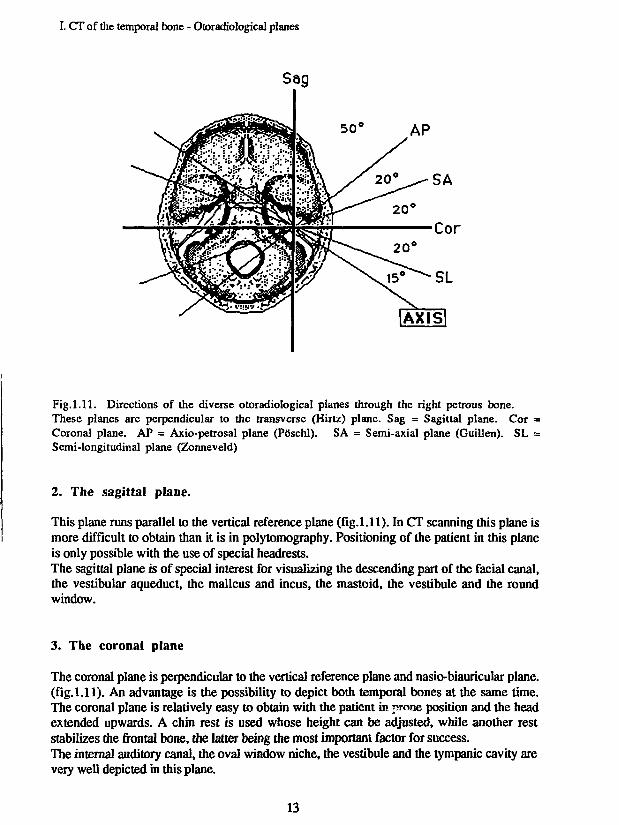
Fig.1.11. Directions of the diverse otoradiological planes through the right petrous bone.These planes are perpendicular to the transverse (Hirtz) plane. Sag = Sagittal plane. Cor =Coronal plane. AP = Axio-petrosal plane (PSschl). SA = Semi-axial plane (Guillen). SL =Semi-longitudinal plane (Zonneveld)
2. The sagittal plane.
This plane runs parallel to the vertical reference plane (fig.l.l 1). In CT scanning this plane ismore difficult to obtain than it is in polytomography. Positioning of the patient in this planeis only possible with the use of special headrests.The sagittal plane is of special interest for visualizing the descending part of the facial canal,the vestibular aqueduct, the malleus and incus, the mastoid, the vestibule and the roundwindow.
3. The coronal plane
The coronal plane is perpendicular to the vertical reference plane and nasio-biauricular plane,(fig.l.l 1). An advantage is the possibility to depict both temporal bones at the same time.The coronal plane is relatively easy to obtain with the patient in prone position and the headextended upwards. A chin rest is used whose height can be adjusted, while another reststabilizes the frontal bone, the latter being the most important factor for success.The internal auditory canal, the oval window niche, the vestibule and the tympanic cavity arevery well depicted in this plane.
13

I. CT of the temporal bone - Otoradiological planes
The coronal plane and the sagittal plane were not frequently used in our study because theycontributed little to the visualization of the details we were especially interested in. Theseplanes have their own indications in other otological disorders (table 1.1).
4. The axio-petrosal plane (Poschl)
The axio-petrosal plane is derived also from the coronal plane. The angle with this plane is 55degrees (= 35 degrees from the vertical reference plane) and perpendicular to the axis of thepetrous pyramid (Pcischl, 1943). In our clinic, however, we use a somewhat different angle forthis plane in order to produce a better imaging of the ossicles: we use an angle of 40 degreesfrom the coronal plane ( = 50 degrees from the vertical reference plane) - (fig. 1.11).This modified axio-petrosal plane is of special interest for visualizing the oval window niche,the superior semicircular canal, the vestibular aqueduct, the geniculate ganglion, the malleus,incus and head of the stapes.
5. The semi-axial plane (Guillen)
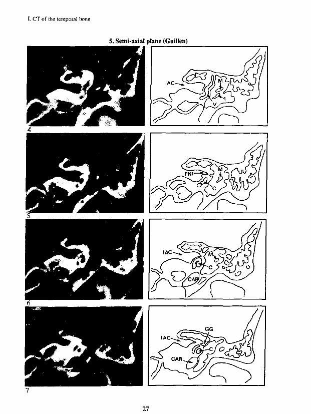
The semi-axial plane (Guillen, 1955) is derived from the coronal plane by rotating the latter20 degrees around the vertical axis in such a direction that the plane subtends an angle of 55degrees with the axis of the petrous pyramid ( = 70 degrees from the vertical reference plane) -(fig.1.11).The oval window niche, the stapes and stapedial footplate, the tympanic cavity (and speciallythe hypotympanum) are well depicted. The promontory and the internal auditory canal can beexamined in this plane as well.
6. The semi-longitudinal plane (Zonneveld)
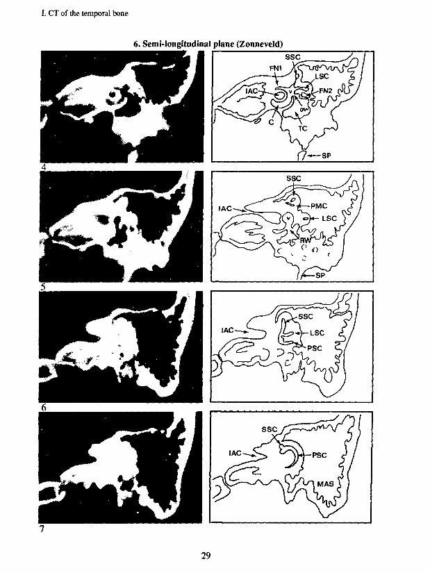
This plane was recently developed in our hospital (Zonneveld et al, 1981). The coronal planeis rotated 20 degrees around the vertical axis to the direction of the pyramidal axis. The angleof this plane with the pyramidal axis is about 15 degrees (fig. 1.11).The semi-longitudinal plane is appropriate for imaging the first and second cochlear turns, theposterior semicircular canal, the internal carotid artery and the vestibule.
In the following section these six otoradiological CT planes are presented with images inseven sequential slices. Scanning sections 1 to 7 are corresponding to the figures in anoverview drawing heading each plane. Scans are accompanied by drawings with abbreviationsof the most important details. A table of legends is given separately (table 1.2).
In table 1.1, a 'visibility matrix' (modified after Zonneveld et al, 1983) shows the optimalscanning planes for visualization of several temporal bone details.
14

CTATLA2
for the
Transverse plane
Sagittal plane
Coronal plane
Axio-petrosal plane
Semi-axial plane
Semi-longitudinal plane

I. CT of the temporal bone
LEGENDS
AAAATCCACARCCCPEACETFCFN1FN2FN3GG
mIACIJBLSCMMASOWPPEPMCPSCRWSSMSPSPNSSSSCTATCTMTSTTTTMVVA
= Antrum= Aditus Ad Antrum= Attic (Recessus Epitympanicus)= Coclea= Cochlear Aqueduct= Carotid Artery= Common Crus= Cochleariform Process= External Auditory Canal= Eustachian Tube= Falciform Crest (Processus Transversus)= Facial Nerve 1st (proximal) part= Facial Nerve 2nd (horizontal) part= Facial Nerve 3rd (vertical) part= Geniculate Ganglion= Hypotympanum= Internal Auditory Canal= Incus= Jugular Bulb= Lateral Semicircular Canal= Malleus= Mastoid= Oval Window= Promontory= Pyramidal Eminence= Petro-Mastoid Canal= Posterior Semicircular Canal= Round Window= Stapes= Stapedius Muscle= Styloid Process= Superficial Petrosal Nerve= Sigmoid Sinus= Superior Semicircular Canal= Tegmen Antri= Tympanic Cavity= Tympanic Membrane= Tympanic Sinus= Tegmen Tympani= Tensor Tympani Muscle= Vestibule= Vestibular Aqueduct
Table 1.2. Legends of the abbreviations in the next six otoradiological planes.
16

I. CT of the temporal bone
VISIBILITY MATRIX
STRUCTURE
- Antrum- Aditus ad Antrum- Attic- Cochlea- Cochlear Aqueduct- Carotid Artery- Cochleariform process- External auditory canal- Eustachian tube- Facial Nerve (proximal part)- Facial Nerve (horizontal part)- Facial Nerve (vertical part)- Geniculate Ganglion- Hypotytnpanum- Incus- Internal Auditory Canal- Jugular bulb- Lateral semicirc. canal- Malleus- Mastoid- Oval window niche- Petromastoid canal- Posterior semicirc. canal- Promontory- Pyramidal process- Round window niche- Sigmoid sinus- Stapes- Superior semicirc. canal- Tegmen antri- Tensor tympani muscle- Tympanic membrane- Vestibular aqueduct- Vestibule
TV
X
X
X
X
X
X
X
X
X
X
X
X
X
X
X
X
X
X
X
X
X
X
X
X
X
X
X
X
X
SG
X
X
X
X
X
X
X
X
X
X
X
X
X
X
X
X
X
X
CR
X
X
X
X
X
X
X
X
X
X
X
X
X
X
X
X
X
AP
X
X
X
X
X
X
X
X
X
X
X
X
X
X
X
X
X
X
X
X
X
X
SA
X
X
X
X
X
X
X
X
X
X
X
X
X
X
X
X
X
X
X
X
X
X
X
SL
X
X
X
X
X
X
X
X
X
X
X
X
X
X
X
X
X
Table 1.1. Visibility matrix of structures in the petrous bone in the diverse otoradiologicalplanes modified according to the matrix of F.W.Zonneveld (1983). In this matrix an Vindicates in which plane each structure can optimally be depicted. TV = Transverse (Hirtz)plane. SG = Sagittal plane. CR = Coronal plane. AP = Axio-Petrosal (Poschl) plane. SA =Semi-Axial (Guillen) plane. SL = Semi-Longitudinal (Zonneveld) plane.
17

I. CT of the temporal bone
1. Transverse plane (Hirtz)
18

I. CT of the temporal bone
1. Transverse plane (Hirtz)
19

I. CT of the temporal bone
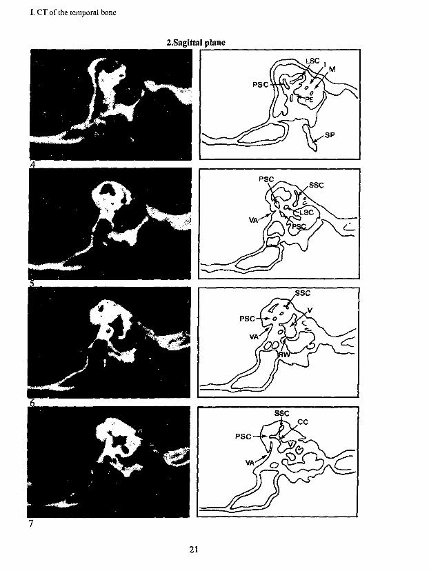
2. Sagittal plane
20
I. CT of ihe temporal bone
2.Sagittal plane
PSC-I
VA'
7ssc
21

I. CT of the temporal bone
3. Coronal plane
22

I. CT of the temporal bone
3. Coronal plane
^ \
FN1| FN2
mvvVEAC
23

I. CT of the temporal bone
4. Axio-peirosal plane (Poschl)
24

I. CT of the temporal bone
4. Axio-petrosal plane (PoschI)
25

I. CT of the temporal bone
5. Semi-axial plane (Guillen)
26
I. CT of the temporal bone
5. Semi-axial plane (Guillen)
27

I. CT of the temporal bone
6. Semi-longitudinal plane (Zonneveld)
28
I. CT of the temporal bone
6. Semi-longitudinal plane (Zonneveld)
29

I. CT of the temporal bone
REFERENCES OF PART I
1. Claus E, Lemahieu SF, Ernould DThe most used otoradiological projections.J Beige Radiol 63: 183-203,1980
2. Dulac MGNote sur la technique de la tomographie du rocherAnn. Otol. Rhinol. Laryngol. 73: 624,1956
3. De Smedt E, Potvliege R, Pimontel-Appel B, Claus E, Vignaud JHigh resolution CT scan of the temporal bone, a preliminary report.J Beige Radiol 63: 205-212,1980
4. Gros CM, Walter JP, Bourjat PTypes et angles de balayage en tomographie de l'oreille interne.Journal de Radiologie et d'Electrologie 46 (10): 641-646,1965
5. Guillen GQuelques apports aux techniques radio-otologiques modernes - L'incidence transorbitaire -La tomographie.Rev Laryngol Otol Rhinol (Bord) 76: 395-446,1955
6. Hanafee WN, Mancuso AA, Jenkins HA, Winter JComputerized tomography scanning of the temporal bone.Ann Otol Rhinol Laryngol 88: 721-728,1979
7. Hirtz EJLe diagnostic radiologique des sinusitisBull, et mem. Soc. de radiol. de France, Paris, 10: 232,1922
8. Johnson GA, Korobkin MImage techniques for multiplanar computed tomography.Radiology 144: 829-834,1982
9. Koracb G, Vignaud JManual of radiographie techniques of the skull.Masson, New York Paris, 1981
10. Littleton JT, Shaffer KA, Callahan WP, Durizch MLTemporal bone: comparison of pluridirectional tomography and high resolution computedtomography.Am J Radiol 137: 835-845,1981
11. Pöschl MDer tomographische Querschnitt durch das Felsenbein.Fortschritte a.d. Gebiete d. Röntgenstrahlen 68:174-179,1943
12. PeysterRGUltra-thin CT imaging: skinny can be beautiful.Diagnostic imaging 89-91, sept. 1983
13. Rettinger G, Kalender W, Henschke FHochauflosungs-Computertomographie des Felsenbeines.Computertomographie 1: 109-116,1981
14. Russell EJ, Koslow M, Lasjaunias P, Bergeron RT, Chase NTransverse axial plane anatomy of the temporal bone employing high spatial resolutioncomputed tomography.Neuroradiology 22:185-191,1982
15. Schneider G, Sager WD, Spreizer HStrahlenbelastung der Orbita bei der Computertomographie mit dem EMI-Scanner CT1010.Fortschr. Röntgenstr. 128 (6): 687-690,1978
30

I. CT of the temporal bone
16. Shaffer KA, Haughton VM, Wilson CRHigh resolution computed tomography of the temporal bone.Radiology 134: 409-414, 1980
17. Shaffer KA, Volz DJ, Haughton VMManipulation of CT data for temporal-bone imaging.Radiology 137: 825-829,1980
18. Swartz JDHigh-resolution computed tomography of the middle ear and mastoid. Part 1: Normalradioanatomy including normal variations.Radiology 148: 449-454,1983
19. Turski PA, Norman D, De Groot J, Capra RHigh resolution CT of the petrous bone: direct vs. reformatted images.Am J Neuroradiol 3: 391-394, 1982
20. Valvassori GELaminagraphy of the ear; pathologic conditions.Am J Radiol 89: 1168-1178,1963
21. Valvassori GE, Mafee MF, Dobben GDComputerized tomography of the temporal bone.Laryngoscope 92 (5): 562-565,1982
22. VignaudJOtoradiology - its current position and future prospects.J Beige Radiol 63: 403-404,1980
23. ZiedsesdesPlantesBGEine neue Methods zur Differenzierung in der Rontgenographie (Planigraphie).Acta Radiol 13:182-192,1932
24. Zonneveid FW, van Waes PFGM, Burggraaf JCT of the semi-longitudinal plane in the petrous bone.Paper 559, presented at the 67th Annual Meeting of the Radiologic Society of NorthAmerica, 1981
25. Zonneveid FW, Damsma HDirect multiplanar CT of the petrous bone.Paper 160, presented at the 68th Annual Meeting of the Radiologic Society of NorthAmerica, 1982
26. Zonneveid FWThe value of non-reconstructive multiplanar CT for the evaluation of the petrous bone.Neuroradiology 25:1-10, 1983
27. Zonneveid FW, Van Waes PFGM, Damsma H, Rabischong P, Vignaud JDirect multiplanar computed tomography of the petrous bone.Radiographics 3: 400-449,1983
28. Zonneveid FW, Vijverberg GPThe relationship between slice thickness ?id image quality in CTMedicamundi 29, no.3,104-117,1984
29. Zonneveid FWThe technique of direct multiplanar high resolution CT of the temporal bone.Neurosurg. Rev. 8: 5-13,1985
30. Zonneveid FWComputed Tomography; Possibilities and impossibilities of an anatomical-medicalimaging techniqueActa Morphol. Neerl.-Scand. 23: 201-220,1985
31

COMPUTED TOMOGRAPHY
INVESTIGATION
OF
THE COCHLEAR CAPSULE
IN
OTOSCLEROSIS

n. CT and Otosclerosis
CONTENTS OF PART II
1. GENERAL CHARACTERISTICS OF OTOSCLEROSIS 351.1. Definition and incidence 351.2. Clinical aspects 35
2. HISTOPATHOLOGY 372.1. Histopathology in otosclerosis 372.2. Other bone diseases involving the labyrinthine capsule 40
3 . TOMOGRAPHY IN OTOSCLEROSIS 41Literature study
4. OBJECTIVES OF THE PRESENT STUDY 45
5. MATERIALS 465.1. Selection criteria 465.2. Patients and ears 475.3. Normal ears used as controls 48
6. METHODS 506.1. Diagnosis of otosclerosis 506.2. Audiometry 506.3. CT-scanning of the labyrinth 506.4. Visual evaluation of CT scans 516.5. Densitometry of the labyrinthine capsule 51
7. RESULTS 567.1. Visual evaluation of the CT images = 567.2. Results of densilometry 607.3. Results of audiometry 737.4. Correlations between bone density loss and inner ear impairment
(bone conduction hearing loss) 75
8. CONCLUSIONS 84
9. DISCUSSION 86
10. REFERENCES 91
34

II. CT and Otosclerosis - Introduction
GENERAL CHARACTERISTICS OF OTOSCLEROSIS
Definition and incidence
Otosclerosis is a genetically determined disease of the bony labyrinthine capsule with adominant mode of inheritance. Only humans are affected. Penetrance is variable. It ischaracterized by bony spongification of the labyrinthine capsule and ossification of theannular ligament, with resultant fixation of the stapedial footplate. Temporal bone studies(Engstrom, 1940; Guild, 1944) showed a histological evidence of otosclerosis in 8.3 - 12percent of whites and in only one percent of negroes. Usually both ears are involved, butunilateral otosclerosis occurs in 10 - 15% of the cases (Schuknecht, 1976). In about 1-2% ofthe cases the condition leads to clinical symptoms (so-called clinical otosclerosis): hearingloss, tinnitus (25%) and in some cases vestibular complaints (5%).
Clinical otosclerosis predominates in females (64 - 72% of all cases), although in temporalbone studies significant difference between males and females could not be found (Engstrom,1940; Guild, 1944). This would indicate that otosclerosis affects females as often as males,but that in females the disease produces clinical symptoms more often. Hormonal factors areconsidered to play a role in this difference: in 63% of female patients the onset or aggravationof hearing loss occurs during pregnancy.
Clinical aspects
In clinical otosclerosis hearing loss may be purely conductive due to ankylosis of thestapedial footplate, caused by an isolated otosclerotic lesion in the oval window region. Amixed conductive-sensorineural hearing loss may exist as a result from stapes fixation incombination with cochlear involvement. In rare cases otosclerosis leads to a puresensorineural hearing loss (Schuknecht, 1976). Clinically, the disease often starts with aconductive hearing loss Ihat later develops into a mixed type loss. Some patients, however,show cochlear involvement from the very beginning.
Usually the tympanic membrane has a normal aspect, unless the patient suffered from otitismedia in the past. The presence of minor atrophic or tympanosclerotic changes, thoughraising the possibility of other diagnoses, does not exclude otosclerosis. The 'Schwarze sign' -a pinkish flush on otoscopic examination - is seen in about 2% of cases, and is due tohyperaemia of the mucoperiosteum over an otosclerotic lesion on the promontory.
One of the classical features of otosclerosis is the symmetry of hearing loss (90%). In earlystapes fixation the air conduction curve is gently rising. In uncomplicated stapedial fixationthis leads, with increasing ankylosis, to a flatter curve with an air-bone gap of about 50 dB.With the passage of time some sensorineural hearing loss usually ensues and a wide variety ofpatterns can result Due to the stapes fixation, a stapedial reflex cannot be evoked.

II. CT and Otosclerosis - Introduction
The bone conduction threshold in otosclerosis does not represent the exact sensorineuralhearing loss in all cases. A part of the bone conduction threshold loss is supposed to be dueto mechanical factors and is known as the so called 'Carhart notch' (Carhart, 1966). Accordingto international standards, this mechanical bone conduction loss amounts to 20 dB. These areaverage values obtained by comparing pre- and postoperative levels and therefore cannot beapplied in individual cases. The bone conduction threshold measurement may be influenced byfactors that are not fully elucidated. Particulary in patients with severe mixed otosclerotichearing loss, a successful stapedectomy can cause a quite considerable gain in bone conductionthreshold so that a considerable so called 'overclosure1 of the air-bone gap takes place. Thisbone conduction gain cannot be explained by the withdrawal of the Carhart notch alone. Otherfactors must be involved. It is unlikely that a successful stapedectomy results in animprovement of cochlear function. It has therefore been claimed that these bone conductiongains are unreal, resulting from the limitations of bone conduction audiometry in measuringbilateral mixed hearing losses.
About 25% of the patients with otosclerosis complain of tinnitus, especially in the elderlywith a mixed type of hearing loss and those with an early onset of cochlear involvement.Excluding vague transient symptoms, definite subjective vertigo is present in only 5 percentof the patients with stapedial or mixed type otosclerosis.
Patients with otosclerosis may exhibit vestibular disturbances. Some patients have periods ofdizziness; caloric hypoexcitability is sometimes found (Virolainen, 1972).
36

II. CT and Otosclerosis - Histopathology
HISTOPATHOLOGY
Histopathology in otosclerosis
Otosclerosis generally occurs as a localized bone disease in which the morphological changesare presumably limited to the labyrinthine capsule. Since otosclerosis involves the oticcapsule and leads in a certain percentage to stapes fixation, it constitutes a complex etiologyfor the impairment of hearing in adults.
The first histological descriptions of otosclerosis are associated with the names of Politzer(1894) and Siebenmann (1912).
In about 85% of the cases, the otosclerotic foci are limited to the oval window region(Guild,1944; Nylen,1949). Other places of predilection are the round window niche, theanterior wall of the internal auditory canal, and in the stapedial footplate. An isolatedlocalization of a focus in the footplate was found in 5 to 12 percent (Guild, 1944; Riiedi &Spoendlin, 1957).
The bony capsule around the membranous labyrinthine system develops rapidly from acartilaginous model with 14 or more ossification centers (Anson, 1973). It may therefore beclassified as cartilage bone although, in some regions, membrane bone takes part in the initialprocess of ossification during fetal development. In the fifth month of intrauterine life thecartilaginous precursor of the labyrinthine capsule has reached adult dimensions andossification centers fuse to form a complete bony capsule in the 23rd week in the cochlearpart. Ossification of the canalicular part occurs more slowly, being completed in the earlypostnatal weeks. Epiphyseal growth does not occur.
The bone is composed of three different layers:a. Periostal (outer) layer, derived from the cambium layer of the periosteum around thecartilaginous capsule. It is similar to the periostal layer of long bones.b. Middle layer, composed of a combination of intrachondral and endochondral bone.c. Endosteal (inner) layer, derived from the endosteum.
The middle and outer layer attain a petrous character, whereas the inner layer remains thin.Despite general change in the fetal period, the islets of intrachondral bone remainhistologically identifiable throughout the adult's life.
The otosclerotic process generally develops in areas of the labyrinthine capsule in whichembryonic cartilage often persists. Generally four phases are recognized in the developmentand progression of otosclerotic lesions in the labyrinthine capsule:
l.Osteolytic phase:This is a lytic or resorption phase (spongiosis) of the otosclerotic lesion caused by lysosomalhydrolases resulting in a destruction of enchondral bone around a vessel and a formation ofresorption spaces containing highly cellular fibrous tissue (Chevance et al, 1970,1972). The
37

II. CT and Otosclerosis - Histopathology
lysosomal hydrolases (i.e.acid phosphatase) break down proteins, DNA, RNA and certaincarbohydrates in an acidic environment. Areas undergoing active resorption are conspicuousdue to the presence of numerous multinuclear giant cells (osteoclasts) and the unusual amountof vascular channels. Mononuclear phagocytes attracted to the surrounding bone of anotospongiotic focus are considered to participate together with osteoclasts in bone resorptionby hydrolase activity (Bretlau et al, 1982).
2. Osteoidformation phase:Reticular cells and fibroblasts assume the formation of osteblasts, resulting in a deposition ofacid mucopolysaccharides and osteoid within the fibroblastic collagen of the resorption spaces.Immature basophilic bone is formed.
3. Remodeling phase:In this phase a remodeling process of new bone formation takes place with the developmentof a more mature acidophilic bone demonstrating a laminated matrix.
4. Mineralization phase:Highly mineralized acidophilic bone with a mosaic-like appearance is formed.
The otosclerotic process can be active or quiescent, while active and inactive areas can besimultaneously present in one otosclerotic focus. Within the lesion, succeeding generations ofbone may be present in an irregular manner. Active lesions can be recognized by their spongystructure and immaturity of osseous tissue as well as by the extent and size of the marrowspaces that contain a very cellular reactive tissue together with numerous giant cells(osteoclasts). A large number of dilated vascular channels are present In the osteoid formationphase resorption spaces are filled with bone which stains with hematoxylin. It gives a bluecolor in the histologic coupes. These 'blue mantles' are not only found in direct continuitywith otosclerotic foci but also in other areas of the otosclerotic bony labyrinth, in particulararound the semicircular canals. Inactive lesions which represent the end stages of the processof otosclerotic bone transformation are identified by solid, lamellar, mosaic-like osseoustissue. It contains a only a few tiny marrow spaces and small blood vessels are occasionallyseen. These new bone deposits are mainly located around the scala tympani of the basalcochlear turn near large active foci of otosclerosis.
Vascular shunts between the vascular system of the otosclerotic lesions and the inner ear havebeen found by Riiedi (1965,1969). He suggested that a venous stasis of blood in these shuntsmay be responsible for a sensorineural hearing loss. Chevance et al (1970,1972) and Bretlauet al (1971), however, believe that toxic products and enzymes play a role in the impairmentof inner ear function. Also atrophy of the stria vascularis and hyalinization of the spiralligament in adjacent active otospongiotic (and less severe in otosclerotic) foci are thought tobe responsible for sensorineural hearing loss (Parahy & Linthicum, 1984).
The original anatomical configuration of the bony labyrinth is usually preserved when thenormal bone is replaced by otosclerotic bone; invasion of the labyrinthine Iumina is rareexcept in very active lesions, while no ingrowth in the internal auditory canal has ever beenfound. As the otosclerotic focus approaches the middle ear surface, the overlying
38
--L
II. CT and Otosclerosis - Histopathology
mucoperiosteum increases in thickness and becomes more vascular. The vascular hyperemiain the superficial layer of the focus and in the overlying mucoperiosteum gives a pinkish hueto a large and actively growing otosclerotic process, as seen through a translucent ear drum(Schwartze's sign).
The inner ear structure most commonly affected by otosclerosis is the spiral ligament,forming the circumferential surface of the membranous labyrinth and lying in direct contactwith the bony labyrinth (Schuknecht & Gross, 1966). More than half of the patients withclinical otosclerosis had foci which were sufficiently large to involve the endosteal layer ofthe labyrinthine lumina. In most of these cases there were atrophic changes in the spiralligament which were more severe than generally seen in this age group. The earliest changesoccurred in the areas adjacent to the otosclerotic bone and consisted of a loss of cellularitywith a deposition of collagen. Such atrophic changes are found in ears not affected byotosclerosis at all. They are considered to be due to aging. Otosclerosis, however, aggravatesthis atrophy: it is most severe in those regions where the spiral ligament is in direct contactwith otosclerotic bone.
The concept of 'cochlear otosclerosis', a pure sensorineural hearing loss caused by otosclerosisof the bony labyrinth without stapes fixation, has been the subject of much discussion(Shambaugh, 1965; Derlacki & Valvassori, 1965); this idea, however, cannot be supported onthe basis of histological studies (Schuknecht & Kirchner, 1974).
Multiple lesions within one and the same temporal bone commonly display similar stages ofactivity. On the other hand, symmetrically located, bilateral lesions may exhibit differentstages of histologic activity. Even the various phases of histologic activity as described abovecan be encountered in one lesion. Very active otosclerotic lesions predominate in youngerindividuals; less active and quiescent forms are more frequendy encountered in older patient. Inthe course of the disease, active otosclerotic lesions tend to proceed steadily towards aninactive terminal stage of histologic stability (Nager,1969).
Parahy & Linthicum (1984) histologically examined 46 temporal bones of patients withotosclerosis. They correlated histological findings with audiometrical data, patient's age atdeath, sex and duration of hearing loss. Mid-modiolar sections through decalcified specimenswere examined by means of light microscopy. Thirty-one bones had one or moreotospongiotic foci and sixteen had otosclerotic foci. The activity of the spongiotic or scleroticlesion adjacent to the spiral ligament was determined by the presence and degree ofhyalinization. Otospongiotic and otosclerotic foci were found side by side at the periphery oflesions and adjacent to normal bone. Atrophy of the stria vascularis and severe hyalinizationof the spiral ligament were found more frequently in combination with otospongiosis thanwith otosclerosis. Generally, otospongiosis has more severe consequences for the auditoryfunction since the degree of hyalinization appears to be strongly correlated with the level ofsensorineural hearing loss. They concluded that otospongiotic and otosclerotic lesions canoccur simultaneously but that it is unlikely that otospongiosis is a preceding stage ofotosclerosis. Absence of hyalinization adjacent to otosclerotic lesions suggests that theselesions were never spongiotic.
39

' II. CT and Otosclerosis - Histopathology
! Other bone diseases involving the labyrinthine capsule<
., rHistologically, otosclerosis resembles certain other bone diseases and since these can alsocause hearing loss, it is not surprising that common aetiological factors have been sought.
1. Ostoegenesis imperfecta (Van der Hoeve & de Kleyn syndrome)This is an inherited disorder of collagen maturation and aggregation that results in defects inall collagen-containing connective tissues. It causes deafness, blue sclerae and brittle bones.About half the children who survive into adult life have or develop a deafness clinicallyresembling otosclerosis. All the ossicles and the labyrinthine capsule are likely to be involvedand more than half of these patients have a marked sensorineural hearing loss.
2. Osteitis deformans (Paget's disease)This is a chronic, progressive bone disorder of unknown cause, characterized by a deformity ofboth the external and internal bony architecture. Microscopically it is characterized by areplacement of the normal bony structure with morphologically and chemically abnormalbone. About 50 percent of patients develop hearing loss due to temporal bone involvement.There is always a sensorineural element accompanied by tinnitus and there are not infrequently
1 vestibular symptoms. In earlier stages of its development a conductive hearing loss mayexist, but in later stages the sensorineural loss progresses and can become subtotal.Audiometric results are similar to those in combined stapedial and cochlear otosclerosis. Thiscondition should be suspected in all cases of 'otosclcrosis' with an age of onset over 45 years.
3. Fibrous Dysplasia of the temporal boneThis is a developmental disorder of the mesenchyme characterized by replacement of bonewith large masses of cellular fibrous tissue containing immature bone spicules and islands ofcartilage. For many years fibrous dysplasia was not distinguished as a separate entity from
i hyperparathyroidism. The lesions of these two disorders are pathologically and radiologicallysimilar, and were formerly known as 'osteitis fibrosa cystica1. Involvement of the temporalbone manifests itself as a swelling in the region of the mastoid and external auditory canal.Radiologically the affected petrous pyramid becomes extremely dense and thick withconsequent asymmetry between the two sides. The outline of the labyrinthine capsule firstbecomes poorly distinguishable from the surrounding bone. Finally it may even disappear asthe lumen of the inner ear structures becomes partially or totally obliterated by a diffusesclerosis of the bone.
4. Osteopetrosis (Albers-Sch0nberg disease; Marble bone disease)Osteopetrosis is a rare bone disorder characterized by abnormal bone growth due to a failure ofresorption of calcified cartilage and primitive bone, resulting in persistence of osteoid tissuein the medullary cavities. Two different forms are described: the benign dominantly inheritedand the malignant recessively inherited form. Children with the latter form usually die at anearly age from anemia or secondary infection (Schuknecht, 1976).The bony labyrinths and ossicles of these patients appear to consist mainly of dense calcifiedcartilage. The mastoids are nonpneumatized. A narrowing of the foramina for the cranialnerves may occur if the skull thickens. Hearing loss is of the combined sensorineural andconductive type.
40

II. CT and Otosclerosis - Literature review
TOMOGRAPHY IN OTOSCLEROSIS
LITERATURE STUDY
The normal labyrinthine capsule appears on polytomographic images as a sharply defined andhomogeneously dense shell, outlining the inner ear lumina. The capsule is normally highlycontrasting with the endolabyrinthine lumina and with the surrounding air cells so that theentire system should always be easily recognizable.
Histological studies proved that, in cases of stapedial (fenestral) otosclerosis combined withsensorineural hearing loss, usually an involvement of the cochlear capsule exists in thedisease process. On the other hand, otosclerotic foci are also found anywhere in thelabyrinthine capsule of autopsy cases that never have been suffering from hearing loss('histological otosclerosis').
Compere (1964) gives a recapitulation of the literature about the results of the studies onpatients with otosclerosis, performed upto 1964 with conventional radiologic techniques. Heradiologically demonstrated certain hyperostotic lesions in the labyrinths of a number ofpatients having otosclerosis with a sensorineural hearing loss; these lesions could be locatedanywhere in the petrous bone, in some instances obscuring the whole labyrinthine system.
Derlacki & Valvassori (1965) tomographically studied patients with a mixed hearingloss due to (surgically confirmed) otosclerosis (20 patients = 40 ears), patients with puresensorineural hearing losses suspected of having cochlear otosclerosis (30 patients = 60 ears)and, as controls, persons with normal hearing and normal audiometric findings (50 persons =100 ears). They categorized the observed radiological changes in three groups which mightrepresent different features of the same disease as it progresses:
1. Type I (or otospongiotic involvement): characterized by a decreased density of the involvedarea of the labyrinthine capsule. It varies from a small dehiscense to larger patchy areas ofradiolucency where the normal anatomical configurations appears completely washed out.2. Type II (or mixed involvement): radiolucent areas mixed with foci of sclerosis of variablesizes; (he dense foci probably represent areas of remineralization as an active focus progressestowards an inactive stage.3. Type III (or diffuse involvement): characterized by a complete loss of contrast between thelabyrinthine capsule and the lumina of the inner ear structures; this loss of contrast could bedue either to extensive remineralization or to diffuse sclerosis of the labyrinthine capsule.
A comparision was made between the radiographic findings and the audiometric results. Thedegree of hearing loss was classified as mild, moderate and severe. In patients with a mixedhearing loss they found changes in the labyrinthine capsule in 90 percent of the cases. In thegroup of patients with sensorineural hearing losses alone (suspected of having cochlearotosclerosis), radiological changes were seen in about 60 percent; these changes were'absolutely identical' with those found in the known cases of mixed hearing loss. The controlshad abnormalities of the labyrinthine capsule in only 6 per cent (Valvassori, 1965).
41

•L
II. CT and Otosclerosis - Literature review
Hoople & Bash (1966) described a hypocycloidal polytomographic technique to visualizeareas of radiolucencies in the labyrinthine capsules of patients with otosclerosis and concludedthat density changes can not be found in all cases with stapedial otosclerosis, but they are infact in many cases. In all such instances there was a sensorineural hearing loss in addition tothe conductive loss which prompted the surgical intervention. They also found that the greaterthe sensorineural part of the hearing loss, the greater were the amounts of bony changeswhich could be seen in the cochlea; these differences were also found between both ears ofpatients with an unequally severe sensorineural hearing loss. In the same petrous bone thereoften were areas of demineralization (spongification) accompanied by areas of excessivemineralization (sclerosis), corresponding with the described stages as seen in histologicstudies.
Valvassori (1966) stated that since the normal labyrinthine capsule is the most dense boneof the human body, it could not become more dense but only eventually thicker by appositionof otosclerotic bone. Spongiotic changes were commonly observed in young patients or inpatients with rapidly progressive sensorineural hearing loss. Cases with a strongly positiveSchwartze's sign always show spongiotic changes when the radiographic findings are positive.He suggested that the spongiotic foci which are radiographically noticeable in the youngpatients become undetectable as they recalcify, so that a 'mature' focus may escape radiologicdetection.
Valvassori & Naunton (1967) examined 90 consecutive cases of surgically provenotosclerosis. Before operation each of these patients recieved a complete audiornetric andradiographic assessment. The audiometric studies included air and bone conduction, pure tonethreshold measurements and speech discrimination tests. The radiographic studies consisted ofmultiple tomographic sections obtained I mm. apart in the frontal and semi-axial projections.They concluded that audiometry is more accurate in evaluating of function, whereasradiography is more precise in assessing the degree of pathological involvement and inpredicting surgical results. Another classification was set up (Valvassori, 1969) to catagorizethe observed radiographic changes according to the extension, degree and type of the process.
Extension1. Changes limited to the capsule of the basilar turn of the cochlea2. Changes diffuse in other portions of the cochlear capsule3. Changes widespread throughout the labyrinthine capsule
Degree (according to the size of the foci of involvement)1. Minimal2. Moderate3. Severe
Type (depending upon the maturation of the process).1. Demineralizing or spongiotic changes2. Sclerotic changes as the result of maturing foci3. Mixed changes
Britton & Linthicum (1970) made antemortem and postmortem polytomes of thetemporal bones in a patient with clinical otosclerosis. They compared these polytomes with
42

II. CT and Otosclerosis - Literature review
histological findings. This comparison indicated that the lesion suspected of beingotosclerosis by x-ray was due to otosclerosis indeed.
Rovsing (1971) summarized the diagnostic value of tomography in cases of otosclerosis asfollows: "The tomographic diagnosis of fenestral otosclerosis is reliable in involvement ofthe vestibular window, the fossula of the vestibular window, the promontory, and to someextent the cochlear window. Tomography not only establishes the diagnosis, but alsoproduces a topographic picture of the degree, the stage, and the extent of otosclerosis. In allfairness it must be added that only changes of a certain degree are visualized in tomograms".
Vignaud (1971) payed more attention to the radiologic appearance of the oval windowniche using Guillen's transorbilal projection and the transverse (Hirtz) projection. She tried tocorrelate the tomographical appearance of the stapedial footplate to its appearance as seen atsurgery. For this study 206 temporal bones were used, all of them with surgically verifiedstages. She had to conclude that a thickening of the stapedial footplate caused by an activeotospongiotic, demineralized lesion could not be seen on tomographical images. However, thethickening of the footplate caused by a sclerotic, highly mineralized lesion could be wellestablished.
Applebaum & Shambaugh (1978) made a histological study of three sets of temporalbones from patients who had antcmortcm polytomographic examinations resulting in adiagnosis of otospongiotic involvement of the cochlea: one of these cases was thought tohave been an example of pure cochlear otospongiosis, whereas the other two cases werepatients with clinical (stapedial) otospongiosis. Their polytomograms were interpreted asunilateral otospongiosis with involvement of the basal cochlear turn. In the first set oftemporal bones no otospongiosis was present. In the other two sets, the otospongiofic lesiondid not involve the cochlea, and a contralateral otospongiotic lesion was present that had notbeen seen on the polytomograms. They concluded that caution must be exercised in theinterpretation of such subtle polytomographic changes in the cochlear capsule; an X-raydiagnosis of pure cochlear otospongiosis should not be given until there is evidence ofcorrelation with pathological materials.
Swartz et al (1984) evaluated 35 consecutive patients having a clinical diagnosis offenestral otosclerosis using high-resolution CT. Abnormal bony excrescenses at or adjacent tothe oval window were found in 26 cases. Scans were made in a transverse and coronal plane.
Mafee et al (1985) evaluated the use of CT for studying cochlear otosclerosis in 32patients with mixed hearing loss and for studying stapedial otosclerosis in 45 patients with amixed or conductive hearing loss. They concluded that CT proved to be more valuable indetermining otosclerotic changes of the oval window and otic capsule than complex motiontomography.
Balli et al (1986) compared preoperative CT data of 8 patients with the peroperativefindings of fenestral otosclerosis and found CT examination in 6 cases to be adequate indetermining the stage of the disease.
43

II. CT and Otosclerosis - Literature review
j Publications from our group
Our first publications on this subject were in 1984. We studied the labyrinthine capsule of 38patients with surgically confirmed otosclerosis by means of high-resolution CT technique(Damsma et al, 1984; Zonneveld et al, 1984). All patients were scanned in atransverse (Hirtz) plane, a semi-axial (Guillen) plane and a semi-longitudinal (Zonneveld)plane in order to visualize changes in the labyrinthine capsule and the oval window niche. Inseven patients ring-shaped zones of radiolucencies were seen around the whole cochlea. Thedensities of these zones were measured and showed a reduction of x-ray attenuation withrespect to the cortical bone ranging between 20 and 50 per cent. Concerning the fenestralotosclerosis, we believed that the spatial resolution of CT is still too limited to give clearanswers about the state of the stapedial footplate and the oval window niche.
We measured the densiues at six fixed locations within the cochlear capsule of patients withcochlear otosclerosis and visible radiolucencies (de Groot et al, 1985). A positivecorrelation was found between the degree of demineralization and the amount of boneconduction bearing loss.
44

II. CT and Otosclerosis - Objectives
OBJECTIVES OF THIS STUDY
As became clear in the previous chapter, the results of polytomographic studies areinconsistent and often incomparable because of the lack of objective reproducible methods.The question is whether otosclerotic foci can be better visualized by high-resolution CTbecause of its better contrast and spatial resolution and its facility to make objective densitymeasurements. Therefore the following problems have been studied:
1. Which otoradiological planes are the most suitable for examining the bony labyrinth and,in particular, the cochlear capsule?
2. What is the density of the normal bony cochlear capsule?a. Is this density the same in the entire cochlear capsule?b. Is this density age-dependent?
3. Is it possible with the present technique to visualize otosclerotic foci?a. In what percentage of ears with otosclerosis can an active focus be detected?b. What is the location and extension of these foci?c. Are there areas of predelection?d. Is it possible to detect 'healed' (remineralized) foci?
4. Are otosclerotic foci with the present technique detectable in clinically non-affected ears ofotosclerosis patients ('unilateral' otosclerosis)?
5. To what extent would density in a certain focus be decreased before being visible by thenaked eye?
6. Since otosclerotic foci in the cochlear capsule are considered to impair inner ear functionthe question arises whether:
a. bone conduction threshold loss is correlated to density loss in a focus.b. bone conduction threshold loss for certain frequencies is correlated to the location of
the foci in the cochlear wall.
45

II. CT and Otosclerosis - Materials
MATERIALS
From 1982 to 1985 a consecutive series of 136 patients with otosclerosis was investigated inthe Departments of ORL and Radiology of the Utrecht University Hospital by CT scanningof both petrous bones in various otoradiological planes as well as by audiometry. Theradiological and audiometrical data of this series of patients were used for this part of thestudy.
1. SELECTION CRITERIA
Inclusion criteria
Included in this study were only the data of patients in whom the clinical diagnosisotosclerosis was confirmed by the presence of stapes fixation during middle ear surgery.
Exclusion criteria
Excluded from this study were the data of patients c.q. ears with:
1. A history or signs of previous otitis media;2. Bone conduction hearing loss of other origin than otosclerosis e.g. noise trauma, infection,sudden deafness, surgical inner ear trauma etc.;3. Vestibular symptoms, and4. An age over 60, except for those in whom no progression of BC hearing loss during thelast 20 years was established. We considered these patients to be not affected by presbyacusis.
46

•-L
. CT and Otosclerosis - Materials
2. PATIENTS and EARS
On the basis of the above mentioned inclusion criteria, 84 patients entered this study. Ofthese, 70 had a bilateral and 14 an unilateral hearing loss due to otosclerosis. The totalnumber of affected ears thus amounted to 154, that of non-affected ears to 14. On the basis ofthe above mentioned exclusion criteria, the data of 20 affected ears and 1 non-affected ear hadto be discarded. The ultimate number of affected ears that were accepted for this study thusamounted to 134; the number of non-affected ears to 13 (Table 2.1).
Otosclerosis Unilateral Bilateral Excluded Included
Patients 14 70 84
Affected ears 14 140 20 134Non-affected ears 14 1 13
Table 2.1. Numbers of patients and ears with otosclerosis accepted for this study.
Age distributionThe age distribution of the 134 examined ears is shown in table 2.2. More than half of theears (N=71) belonged to patients in the age groups of 31-50 years. Ears of patients in the agegroup of 61 to 70 years were only included when the audiograms showed no progression inBC hearing loss during the last 20 years. These 16 ears were considered to be not affected bypresbyacusis.
Patients' age 11-20 21-30 31-40 41-50 51-60 61-70
Numbers of ears 2 19 38 33 26 16
Table 2.2. Age distribution of the 134 ears of patients with otosclerosis fulfilling theselection criteria. More than half of the ears (71) were ears of patients between 3 1 - 5 0 years ofage.
Sex distributionFrom the 84 patients included, 35 were male (4 with unilateral and 31 with bilateralotosclerosis) and 49 female (10 with unilateral and 39 with bilateral otosclerosis) - (table 2.3).
Otosclerosis Male Female Total
Unilateral otosclerosis 4 10 14Bilateral otosclerosis 31 39 70
Total 35 49 84
Table 2.3. Sex distribution of the patients.
47

--L
II. CT and Otosclerosis - Materials
3. NORMAL EARS USED AS CONTROLS
As controls, CT scans of 35 otologically normal ears of 23 patients (9 males, 14 females)were used (table 2.4). 11 of these ears were the healthy, contralateral ears of patients withunilateral chronic otitis media, middle ear trauma, acoustic neurinoma, sudden deafness andcongenital deafness. The non-affected ears of patients with unilateral Meniere's disease werenot used as controls. The other 24 control ears belonged to 12 patients in whom CTscanning was carried out and no otological or vestibular disorder was found e.g. Bell's palsy,otalgia, dizziness of central origin etc.
Normal (control) ears Patients Male Female Ears
Contralateral ears 11 5 6 11Both ears 12 4 8 24
N= 23 9 14 35
Table 2.4. Numbers of patients and ears used as controls.
Age distribution
The age distribution of the control ears is given in table 2.4.a
Patients' age 1-10 11-20 21-30 31-40 41-50 51-60 61-70
Numbers of ears 3 2 5 13 4 6 2
Table 2.4.a. Age distribution of the 35 control ears.
48

II. CT and Otosclerosis - Materials
SUMMARY
PATIENTS WITHSURGICALLY CONFIRMED
OTOSCLEROSIS84
BILATERALLYAFFECTED
70
UNILATERALLYAFFECTED
14
NORMAL (CONTROLS)
23
BILATERAL
12
INCLUDED
UNILATERAL
11
CONTROLSNORMAL EARS
35
35
Fig.2.1. Composition of the materials (ears with otosclerosis and control ears).
49

n. CT and Otosclerosis - Methods
METHODS
1. DIAGNOSIS
The diagnosis otosclerosis was made on the basis of:
1. The history of a (slowly) progressive hearing loss without an evident ear disease,2. A normal tympanic membrane,3. A conductive or mixed hearing loss at audiometry,4. The absence of a stapedial reflex, and5. A stapedial footplate fixation at surgery.
2. AUDIOMETRY
In all patients and controls, tone and speech audiometry as well as tympanometry andstapedial reflex measurement was performed on both ears. In this study only pure toneaudiometric data were used. In order to avoid influences of possible cochlear injury caused bysurgery, only the preoperative audiograms were used to correlate with CT findings.
Pure tone threshold audiograms for air and bone conduction were made for all octavefrequencies from 125 through 8000 Hz in a sound proof anechoic room using a Madsen OB 8.All patients underwent tone audiometry twice before surgery. Masking of the non-test ear wascarried out according to the technique of Hood. When a threshold difference of IS dB or morebetween two subsequent octaves was found, threshold was also measured at the intermediatefrequency.
3. CT-SCANNING OF THE LABYRINTH
Philips Tomoscan 310/350
All patients were scanned by means of a Philips Tomoscan 310/350 high resolution CTscanner, experimentally equipped with a table swivel (part I). A spatial resolution of 0.6 mmwas obtained by using the principle of geometrical enlargement: the petrous bone wasenlarged to an 8 cm square field of view by means of a zoom reconstruction. The sharpness ofthe images was enhanced by using 1200 projection directions in a 9.6 sec scan time and aRamp convolution filter. To avoid degradation of the sharpness by partial volume averaging,a slice thickness of 1.5 mm was used. For display and photography a window level of 300 Hand a window width of 3200 H were selected. The scans were made at 120 kV and 480 mAs,resulting in a peak skin dose of about 80 mGy.
50

-i
II. CT and Otosclerosis - Methods
Planes of examination
The petrous bones of all patients and control subjects were scanned in two or moreotoradiological planes. The transverse (Hirtz) plane was used in each case and served as astarting point for further examination. The second (and third) plane was chosen depending onthe specific question.
The semilongitudinal (Zonneveld) plane was taken as the second plane of examination in themajority of cases, as it gives an exellent imaging of the vestibule, the first cochlear turn andthe superior semicircular canal. Together with the transverse plane it provides an almostcomplete picture of the entire labyrinthine capsule.
The semi-axial (Guillen) or axio-petrosal (PSschl) plane were preferred as the second plane ofexamination when the oval window niche had to be examined, e.g.,- for checking the position of a stapes prosthesis before revision surgery,- suspected obliteration of the oval window niche or an overhanging facial nerve.
4. VISUAL EVALUATION OF CT SCANS
All CT images were visually evaluated independently by a radiologist (H. Damsma), aphysicist (F.W. Zonneveld) and an otorhinolaryngologist (the author). Not only the cochlearcapsule, but the entire labyrinthine capsule was searched in order to detect foci of densityloss. Therefore, we used CT-scans of both transverse and semilongitudinal (semi-axial oraxio-petrosal) planes.
5. DENSITOMETRY OF THE COCHLEAR CAPSULE
In otosclerosis we are especially interested in the cochlear part of the labyrinth. Thereforedensity measurements were carried out in the cochlear capsule.
5.1. Determination of the maximum capsular density
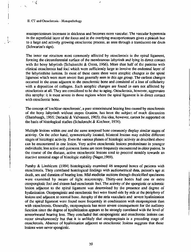
In determining the density range of the cochlear capsule, the values of maximum andminimum density were measured in each ear. The Philips Tomoscan 310/350 has a softwarefeature which enables us to compare each pixel of the image with a reference H-value (leveldetection). This reference H-value can be varied over the whole density range. Each pixel ofthe image with the same H-value as the reference is highlighted on the screen (fig.2.2). In thisway points of isodensity can be visualized at each reference H-value.
With this method, determination of the maximum density appeared to be relatively easy andwell reproducible. The reference value is increased until only one or two highlighted pixels
51
II. CT and Otosclerosis - Methods
remain visible on the screen, pixels with the highest H-value. This technique was used ineach slice of the applied otoradiological planes. After examining all CT scans, the highestH-value ever found in the cochlear capsule was considered to be the maximum capsulardensity.
Fig.2.2. Determination of the maximum density (highest H-value) in the cochlear capsule.
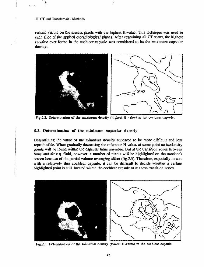
5.2. Determination of the minimum capsular density
Determining the value of the minimum density appeared to be more difficult and lessreproducible. When gradually decreasing the reference H-value, at some point no isodensitypoints will be found within the capsular bone anymore. But at the transition zones betweenbone and air c.q. fluid, however, a number of pixels will be highlighted on the monitor'sscreen because of the partial volume averaging effect (fig.2.3). Therefore, especially in earswith a relatively thin cochlear capsule, it can be difficult to decide whether a certainhighlighted point is still located within the cochlear capsule or in these transition zones.
Fig.2.3. Determination of the minimum density (lowest H-value) in the cochlear capsule.
52
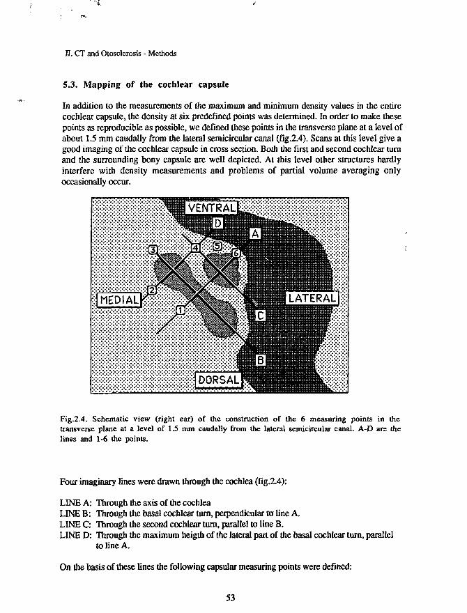
•i
II. CT and Otosclerosis - Methods
5.3. Mapping of the cochlear capsule
In addition to the measurements of the maximum and minimum density values in the entirecochlear capsule, the density at six predefined points was determined. In order to make thesepoints as reproducible as possible, we defined these points in the transverse plane at a level ofabout 1.5 mm caudally from the lateral semicircular canal (fig.2.4). Scans at this level give agood imaging of the cochlear capsule in cross section. Both the first and second cochlear turnand the surrounding bony capsule are well depicted. At this level other structures hardlyinterfere with density measurements and problems of partial volume averaging onlyoccasionally occur.
:£::&:£:££:£
:J MEDIAL££:;•£:£:£:£:;
v::::::::x:x:x::'-:'
m&
^v'xXvX;
• : • : • : • : • : • ! • : • : • : •
BVENTRALEa;
lilllllllllHH|:[DORSAL|
lllllllllllllllllllfffflMllfffL-'-'^-
^BILATERAL 1:;;:
iiiiiiiiiiiiiiiP***'-'-'''
Fig.2.4. Schematic view (right ear) of the construction of the 6 measuring points in thetransverse plane at a level of 1.5 mm caudally from the lateral semicircular canal. A-D are thelines and 1-6 the points.
Four imaginary lines were drawn through the cochlea (fig.2.4):
LINE A: Through the axis of the cochleaLINE B: Through the basal cochlear turn, perpendicular to line A.LINE C: Through the second cochlear turn, parallel to line B.LINE D: Through the maximum heigth of the lateral part of the basal cochlear turn, parallel
to line A.
On the basis of these lines the following capsular measuring points were defined:
53

II. CT and Otosclerosis - Methods
Point 1: On line A (cochlear axis) just above the fundus of the internal auditory canalPoint 2: On line D medially from the basal cochlear turnPoint 3: On line B at its anterior cross-section through the capsulePoint 4: On the crossing of the lines C and DPoint 5: At the midpoint between points 4 and 6Point 6: On line A near the cochlear apex
The software of the Philips Tomoscan 310/350 facilitates drawing a line between two markedpoints with a lightpen on the screen. A diagram then shows the H-values of all pixels on thatline. In putting the lightpen on a point on this diagram, the corresponding H-value is givenon the screen.
This method was used to locate the predefined fixed points in the cochlear capsule in order todetermine the H-value of each point correctly. In figs. 2.6 to 2.11 the measurement of points1 to 6 are shown, making use of this method.
During the densitometric study it became evident that point 1 could not be measuredaccurately enough in all cases because of the partial volume averaging effects. This was due tothe very close proximity of the internal auditory canal. Density measurements at point 6offered a similar problem, as the cochlear capsule at the level of the apex is often too thin toperform reliable measurements. For these reasons the density values at point 1 and 6 wereexcluded from the final analysis of the data.
Measurements at points 2, 3,4 and 5 yielded reproducible values and these were used forfurther study of the degree of capsular density loss in relation to the amount of boneconduction hearing loss.
As one pixel contains the H-value of a piece of tissue (voxel) sized 0.3 x 0.3 x 1.5 mm, wemeasured the mean H-value of 4 pixels, in order to measure in a larger volume (about 0.5mm3) than that of just one voxel. The size in the z-direction (1.5 mm) depends on the slicethickness (fig.2.5).
0.6 mm
mm
-0.3 mm
1.5 mm
— 0.6 mn
1.5 mm
Fig.2.5. Density measurements in the 6 predefined points were performed in a volume of 4voxels.
54

II. CT and Otosclerosis - Methods
In figs. 2.6 - 2.11 the method of determining the location of the 6 predefined points isillustrated. This procedure appeared to be accurate and reproducible (except for the points 1 and6). Repeated measurements at the points 2 to 5 gave variations of less than 30 H.
Fig.2.6. Measurement of point 1 Fig.2.7. Measurement of point 2
Fig.2.8. Measurement of point 3 Fig.2.9. Measurement of point 4
Fig.2.10. Measurement of point 5 Fig.2.11. Measurement of point 6
55

II. CT and Otosclerosis - Results
RESULTS
I. VISUAL EVALUATION OF THE CT IMAGES
1.1. Normal (control) ears
On visual evaluation the labyrinthine capsules of all 35 normal control ears had a regular andhomogeneous aspect in all scans of the applied planes (transverse, semi-longitudinal, axio-petrosal and semi-axial plane).
1.2. Ears with otosclerosis
The results of the visual evaluation of the scans of the 84 patients with surgically confirmedotosclerosis were as follows:
In 68 patients (81%) a normal labyrinthine capsule was seen in all scans of both temporalbones: the bony labyrinthine capsules appeared homogeneous and dense without anyirregularity, giving no suspicion of the existence of demineralization activity.
In 16 patients (19%) radiolucent areas were present in the labyrinthine capsule. In 13 patientsthe disorder was bilateral, in 3 patients unilateral (table 2.5).
Radiolucencies Patients Ears
Bilateral 13 26Unilateral 3 3
Total 16 29
Table 2.5. In 13 patients radiolucencies were seen in both ears, in 3 patients in one ear.
Two types of radiolucency could be distinguished: the 'ring type' and the 'patchy type'. Single,isolated foci were not encountered.
56
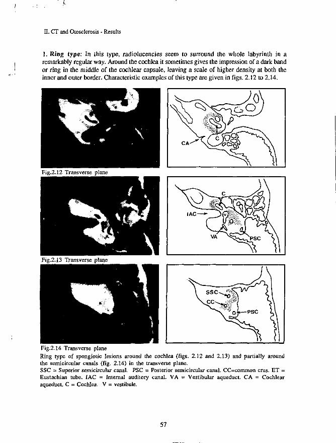
II. CT and Otosclerosis - Results
1. Ring type: In this type, radiolucencies seem to surround the whole labyrinth in aremarkably regular way. Around the cochlea it sometimes gives the impression of a dark bandor ring in the middle of the cochlear capsule, leaving a scale of higher density at both theinner and outer border. Characteristic examples of this type are given in figs. 2.12 to 2.14.
Fig.2.12 Transverse plane
Fig.2.13 Transverse plane
Fig.2.14 Transverse planeRing type of spongiotic lesions around the cochlea (figs. 2.12 and 2.13) and partially aroundthe semicircular canals (fig. 2.14) in the transverse plane.SSC = Superior semicircular canal. PSC = Posterior semicircular canal. CC=common cms. ET =Eustachian tube. IAC = Internal auditory canal. VA = Vestibular aqueduct. CA = Cochlearaqueduct. C = Cochlea. V = vestibule.
57

II. CT and Otosclerosis - Results
2. Patchy type: In this type, areas of radiolucency are found more spread over the entirelabyrinthine capsule and seem to be more irregular in shape and size. These radiolucent areassometimes coalesce into larger lesions and can reach the periphery of the labyrinthine capsuleand/or the border of the labyrinthine cavities (fig. 2.15 - 2.17).
Fig.2.15. Semi-longitudinal plane
Fig.2.16. Semi-longitudinal plane
Fig.2.17. Semi-longitudinal planePatchy type of spongiotic lesions in the labyrinthine capsule.SSC = Superior semicircular canal. LSC = Lateral semicircular canal. IAC = Internal auditorycanal. FN1 = Facial nerve (first part). C=coclea V=vestibule.
Two patients with bilateral radiolucencies had hearing loss in one ear caused by other factorsthan otosclerosis. These two ears were excluded from the study. Therefore the total number of
58

IT. CT and Otoselerosis - Results
ears with foci of visible density loss amounted to 27. Table 2.6 gives the numbers of patientsand ears with and without visible radiolucencies as found in the 84 patients with surgicallyconfirmed otosclerosis.
Ears with otosclerosis Patients Ears
Normal labyrinthine capsules 68Radiolucencies in the capsule 16
10727
Total 84 134
Table 2.6. Results of the visual evaluation of CT scans of the labyrinthine capsule in 134 earsof 84 patients with surgically confirmed otosclerosis.
1.3. Non-affected ears of patients with otosclerosis
In the 13 unaffected ears of patients with unilateral surgically confirmed otosclerosis, nochanges could be found in the homogeneity of the cochlear capsule. At the visual evaluationof the CT images there was no difference in opacity when compared to the 35 control ears.
2. SUMMARY OF THE VISUAL EVALUATION
In table 2.7 the results of the visual evaluation (examination by the naked eye) of theCT-scans in all three groups (control ears, affected and non-affected ears) are summarized. Allcontrol ears (N=35) had homogeneous labyrinthine capsules. The same applied for thenon-affected ears of patients with otosclerosis (N=13). The affected ears (N=134) showed fociof demineralization in 27 cases. The other 107 ears had no visible radiolucencies in thelabyrinthine capsules.
Visual evaluation N No radiolucencies Radiolucencies
Control ears 35Affected ears 134Non-affected ears 13
35107
13
027
0
Table 2.7. Results of the visual evaluation of the labyrinthine capsules in normal ears and inaffected and non-affected ears of patients with surgically confirmed otosclerosis.
59

II. CT and Otosclerosis - Results
2. RESULTS OF DENSITOMETRY
2.1. NORMAL (CONTROL) EARS.
Maximum and minimum density
The maximum and minimum density values in the bony cochlear capsule measured in the 35normal (control) ears are given in fig.2.18 in a random arrangement. Both maximum andminimum density are represented in a line graph and show a relatively small variation. Themean maximum density value appeared to be 2055 H with a standard deviation of 74. Themean minimum density was found to be 1804 H (standard deviation: 65). Table 2.7 gives thenumerical data of the mean maximum and minimum density with their standard deviations.From these data it may be concluded that both maximum and minimum density in the normalhuman cochlear capsules show very little interindividual variation.
NORMAL (CONTROL) EARS
H2500MAX
2000 r A 2 _ ? r t ~ 2~~ 2 ~
1500 4 " MIN
1000
500
0 » i i i i i i i i i i i i i i i i i i i i i ; i i i i i i i i i i i i
1 35
Fig.2.18. Maximum and minimum density in the cochlear capsules of 35 normal (control) ears.On the X-axis the ears 1 to 35 are shown. The Y-axis gives the density value in Hounsfieldunits (H).
Control ears (N=35) Mean SD
Maximum density 2055 74Minimum density 1804 65
Table 2.7. Mean maximum and mean minimum density in 35 normal (control) ears.
60

II. CT and Otosclerosis - Results
Density at predefined points 2, 3, 4, 5
The results of densitometry in the normal (control) ears measured at the predefined points 2-5are presented in table 2.8. No statistically significant difference in density values betweenthese four points could be found (p>0.05). The mean density of these four points appeared tobe 1898 H (SD: 55). From these data can be concluded that in normal ears the bony cochlearcapsule has a homogeneous radiodensity of about 1900 H with a very small interindividualvariation.
Normal ears (N=35) Mean SD
Point 2 1887 54Point 3 1897 76Point 4 1925 70Point 5 1884 72
Table 2.8. Mean density values at the predefined points 2-5 in the cochlear capsule of 35normal (control) ears.
Relation with age
Both maximum and minimum capsular density were found to have no correlation with age.The coefficient of the correlation between maximum density and age was 0.13 and statisticallynot significant (p>0.05).The coefficient of the correlation between minimum capsular density and age was 0.11 andnot significant either (p>0.05).
61

II. CT and Otosclerosis - Results
2.2. AFFECTED EARS OF PATIENTS WITH OTOSCLEROSIS
Maximum and minimum density
The maximum and minimum density values measured in the cochlear capsules in 134affected ears of patients with surgically confirmed otosclerosis are presented in table 2.9.
Affected ears <N=134) Mean SD
Maximum density 2094 75Minimum density 1576 350
Table 2.9. Mean maximum and minimum density in 134 affected ears of patients withotosclerosis.
The mean maximum density turned out to be 2094 H (SD = 75) and differed significantly(p<0.006) with the values measured in the control ears (2055 H, SD:74). The maximumcapsular density in ears with otosclerosis is about 40 H higher than normal.
The mean minimum density appeared to be much lower (1576 H) as compared to that of thecontrol ears (1804 H). This difference is highly significant: p<0.001. The variation of theminimum density value in the ears of patients with otosclerosis appeared to be much larger(SD = 350) than that of the control ears (SD = 65).
Density at the predefined points 2, 3, 4, 5
As occurred with the minimum density, a similarly wide variation in H-values was found atmeasuring points 2-5. The mean H-values of these points was lower in the patients' ears thanin the control ears (table 2.10). Due to the higher standard deviation, the significance of thesedifferences was very low for point 2 (p=0.03) and absent for the other points (p>0.05).The interindividual density of these four points did not differ significantly as well.
Affected ears (N=134) Mean SO
Point 2 1769 318Point 3 1835 259Point 4 1822 308Points 1805 323
Table 2.10. The mean density at points 2-5 in the cochlear capsule of 134 affected ears ofpatients with otosclerosis.
62

'-L
II. CT and Otosclerosis - Results
Correlation between age and minimum density
In fig.2.19 the correlation between minimum density and age in these ears is shown. A lowpositive correlation is present (R=0.26; p<0.01). Minimum capsular density seems to beslightly increasing with age.The correlation between maximum density and age had a low significance (R=0.20; p<0.05).
H 3000
2000 -
1000-
Fig.2.19. Correlation (linear regression) between age and minimum density in 134 affected earsof patients with otosclerosis. Correlation-coefficient = 0.26 (p < 0.01).
63

II. CT and Otosclerosis - Results
Categories of minimum density
In contrast to maximum density, minimum density values showed a wide variation (from 510to 2012 H). Because of this variation we grouped the ears into three categories of minimumdensity. The mean minimum density in normal (control) ears (1804 H, SD: 65) was taken asa reference. Minimum density was considered to be normal when the H value lies in the rangeof 1804 plus and minus twice the standard deviation (1674 -1934 H) - (fig.2.20).
H2500
2000<
1500 •
1000
500
INCR.
DENS.
N=9
AFFECTED EARS
NORMAL MINIMUM DENSITY
N=50
MAX
MIN
0 1111111 111111 ill 11 11 ill I ill 111 1111II111 I I 111111111111 1111111 9 59
DECREASED MINIMUM DENSITY
N=75
0 liiiiiiiiiniiiiiiiiiiiiiiiiiiiiiiiiiiiiiiiiniiiiiiiiiiiiiiiiiiiiiiiiiiin
60 134
Fig.2.20. Maximum and minimum capsular density of all 134 affected ears of patients withotosclerosis, arranged according to the value of minimum capsular density. The upper diagramshows the affected ears with an increased (1-9) and normal (10-59) minimum density, the lowerdiagram the ears with a decreased (60-134) minimum density.
64

. CT and Otosclerosis - Results
In fig.2.20 the maximum and minimum density of all 134 ears are given in the order of theminimum density value. The following three categories were distinguished:Ears with an increased minimum density (>1934 H), ears with a normal minimum density(1674 -1934 H) and ears with a decreased minimum density (<1674 H)
The numbers of ears and the percentages in the three categories are given in table 2.11:
Minimum density H N %
IncreasedNormalDecreased
Total 134 100
Table 2.11. Numbers and percentages of affected ears in the three categories according to thevalue of the minimum capsular density (N = 134).
The mean age of patients having ears with an increased minimum density appeared to behigher (55 years) than that of ears with a normal minimum density (46 years) and decreasedminimum density (43 years). This difference is significant (p<0.001) between ears withincreased minimum density and ears with normal or decreased minimum density. Between theears with normal minimum density and ears with decreased minimum density no significancecould be found in the difference of age (p>0.05)
Minimum density Mean age (years)
>19341674-1934<1674
95075
73756
Increased 55Normal 46Decreased 43
Table 2.12. Mean age of the patients' ears in the three categories.
This means that the ears with an increased minimum capsular density belonged to olderpatients, whereas a normal or decreased minimum capsular density was found in younger
' - with otosclerosis (table 2.12).
65

21791978
2036205020562036
4219
41375054
II. CT and Otosclerosis - Results
EARS WITH INCREASED MINIMUM DENSITY ( > 1934 H)
In the 9 ears with increased minimum density (table 2.13), the mean maximum H-value washigher than the normal maximum density. Despite the small number of ears this differenceappeared to be statistically significant (p<0.001). The H-values at the predefined points 2-5were also higher than normal with a small variation (SD < 55); there was no significantdifference in H-value between the points (p>0.05).
Ears with increased minimum density Mean SD
Maximum densityMinimum density
Point 2Point 3Point 4Point 5
Table 2.13. Mean density values with standard deviations for ears with increased minimumdensity (N=9).
EARS WITH NORMAL MINIMUM DENSITY (1674-1934 H)
The number of ears with a normal minimum capsular density amounted to 50. Maximumdensity was significantly higher than normal (p<0.01). Density values of the points 2-5 didnot differ significantly from normal (p>0.05); their variation was small, although somewhatlarger than in normal ears (table 2.14). No significant differences in H-value were presentamong the points (p>0.05).
Ears with normal minimum density Mean SD
Maximum densityMinimum density
Point 2Point 3Point 4Point 5
Table 2.14. Mean density values with standard deviations for ears with normal minimumdensity (N=50).
66
21031790
1910191719011915
5773
931039682

20791384
1644175417191714
81359
372311371400
II. CT and Otosclerosis - Results
EARS WITH DECREASED MINIMUM DENSITY ( < 1674 H)
In 75 ears minimum density in the cochlear capsule was found to be lower than normal. Themean maximum capsular density showed no significant difference with that of the control ears(table 2.15).The densities at the four points were lower than normal but showed no significant point topoint difference with each other (p>0.05).
A correlation between minimum density and age was not found (R=0.27; p>0.05).
Ears with decreased minimum density Mean SO
Maximum densityMinimum density
Point 2Point 3Point 4Point 5
Table 2.15. Mean density values with standard deviations for ears with decreased minimumdensity (N=75).
Standard deviations of minimum capsular density and of the densities at the predefined points2-5 are high (311-400) as compared to those of ears with increased and normal minimumdensity. The standard deviation of the maximum density (SD=81) is small and of about thesame magnitude as that of ears with increased and normal minimum density. Regarding thecurve of the minimum density in fig. 2.20, a rather sharp deviation can be recognized at aH-value of about 1500 H. This means that ears with minimum density values lower than ±1500 H have a much wider spreading. Maximum density remains rather constant, whileminimum density varies widely. The density range (difference between maximum andminimum density) thus increases. With this increase in density range, the visibility ofradiolucencies on CT-scans could increase because of a higher contrast between maximum andminimum density values.
All but two of the 27 ears with visible radiolucencies on CT-scans appeared, when examinedby densitometry, to have minimum capsular densities below 1500 H. These two exceptionshad a minimum density slightly higher than 1500 H. In one case minimum density wasbelow 1500 H and showed no visible radiolucencies on the scans. In the other 26 earsmaximum capsular density does not follow the decay in minimum density as seen in fig.2.20: density range increases.
Interpretation of the 'kink' in the curve of fig.2.20 is difficult. The ears are sequentiallyarranged according to the value of the minimum density. In 26 of the 75 ears with decreasedminimum density (about 35%) this minimum density is lower than 1500 H, and areas of
67

II. CT and Otosclerosis - Results
density loss are visible on CT-scan, whereas in the other 65% CT-scans look normal.Visibility of density loss seems to depend on a combination of a low minimum capsulardensity (<1500 H) and a wide density range.
These findings make the ears with a minimum density between 1500 and 1674 H moreinteresting: they generally do not show disorders on CT-scans by visual examination and aretherefore not distinguishable from normal ears or from affected ears with a minimum densityin the normal range (1674 -1934 H). Nevertheless, they have decreases in minimum densityand must be considered as ears with density losses in the cochlear capsules. For this reason wehave split up the group of ears with a decreased minimum capsular density into twosubgroups: ears with a moderately decreased minimum capsular density and those with aseverely decreased one. Fig. 2.21 presents the subdivision of the 134 ears affected byotosclerosis schematically.
MINIMUM DENSITYINCREASED
N=9
AFFECTED EARSN = 134
MINIMUM DENSITYNORMAL
N=50
MINIMUM DENSITYDECREASEDN=75
MODERATELYDECREASED
N=49
SEVERELYDECREASED
N=26
Fig.2.21. Different categories of affected ears of patients with otosclerosis.
68

20911616
1835187818851920
5838
131111104108
n. CT and Otosclerosis - Results
EARS WITH MODERATELY DECREASED MINIMUM DENSITY (1500-1674 H)
OF the 75 ears with decreased minimum capsular density, 49 had minimum H values between1500 and 1674. These ears are located on the left side of the kink in the curve of fig.2.20. Themean minimum density (1616 H) showed a small spreading (SD: 38). Mean maximumdensity was found to be 2091 H with a standard deviation of 58 (table 2.16) which iscomparable with that of the control ears. The densities at the four predefined points showed nosignificant differences with each other (p>0.05) except between points 2 and 5 (p<0.001).A correlation between minimum density and age could not be estimated (R=0.27; p>0.05).
Moderately decreased minimum density Mean SD
Maximum densityMinimum density
Point 2Point 3Point 4Point 5
Table 2.16. Mean density values (H) in ears with a moderately decreased minimum density(N=49).
EARS WITH SEVERELY DECREASED MINIMUM DENSITY ( < 1500 H).
In 26 ears very low values of minimum density were measured. The average was 948 H witha standard deviation of 275 H. The H-values at the predefined points were very widespread(table 2.17). The mean maximum density, however, did not differ significantly from thevalues in the control ears (p>0.05). No differences in H-values could be found between thepredefined points (p>0.05) except between those of point 2 and 3. This difference had a lowsignificance (p<0.05). All ears of this group showed areas of density loss within the cochlearcapsules at the visual examination of the CT-scans.No correlation could be found between age and minimum density (R=0.01; p>0.05)
Severely decreased minimum density Mean SD
Maximum densityMinimum density
Point 2Point 3Point 4Point 5
Table 2.17. Mean density values (H) in ears with severely decreased minimum density (N=26).
69
2055948
1283152114071326
109275
411419480461

II. CT and Otosclerosis - Results
2.3. NON-AFFECTED EARS OF PATIENTS WITH OTOSCLEROSIS.
In 14 patients with surgically confirmed otosclerosis the disease was clinically manifest inonly one ear. The contralateral non-affected ears of these patients were analyzed in the sameway as the affected ears. One ear had to be excluded because of intercurrent otitis media.
Maximum and minimum density
The mean maximum density turned out to be 2092 H (SD: 61), the mean minimum density1841 H (SD: 68). These values showed no significant differences with those of the normalcontrol ears (p>0.05) - (Fig. 2.22 and table 2.18).
NON-AFFECTED EARS
H2500 MAX
Fig.2.22. Maximum and minimum density in clinically non-affected ears of patients withunilateral otosclerosis (N=13).
Non-affected ears (N=35) Mean SD
Maximum densityMinimum density
20921841
6168
Table 2.18. Mean maximum and minimum density in non-affected ears (N=13).
70

i • . I
1931194819701915
84776985
II. CT and Otosclerosis - Results
Density at the predefined points 2, 3, 4, 5
Density values at the predefined points 2-5 were somewhat higher than those in normal ears,but the significance of this difference appeared to be low for points 2-4 (p<0.05) and absent inpoint 5 (p>0.05). The standard deviations were of the same magnitude as in normal ears andin affected ears with increased and normal minimum density (table 2.19).
Non-affected ears (N=13) Mean SD
Point 2Point 3Point 4Point 5
Table 2.19. Mean density at the points 2-5 of clinically non-affected ears of patients withunilateral otosclerosis (N=13).
Relation with age
Minimum density appeared to be moderately correlated with the age of the patients (R=0.59)but the significance of this correlation was low (p<0.05).
2.4. SUMMARY OF THE DENSITOMETRIC RESULTS
The complete results of the densitometry for the normal (control) ears as well as for theaffected and non-affected ears of patients with otosclerosis are summarized in the tables 2.20 -2.22.
EARS
MaximumMinimum
Point 2Point 3Point 4Point 5
CONTROLS
2055 (74)1804 (65)
1887 (54)1897 (76)1925 (70)1884 (72)
AFFECTED
2094 (75)1576 (350)
1769 (318)1835 (259)1822 (308)1805 (323)
NON-AFF.
2092 (61)1841 (68)
1931 (84)1948 (77)1970 (69)1915 (85)
N= 35 134 13
Table 2.20. Summary of the results of densitometry for normal (control) ears and for affectedand non-affected ears of patients with otosclerosis. All numbers represent mean density inHounsfield values (H). Numbers in parentheses are standard deviations.
71

II. CT and Otosclerosis - Results
AFFECTED EARS
MIN. DENSITYRANGE (H)
MaximumMinimum
(N=134)
INCREASED>1934
2179 (42)1978 (19)
NORMAL1674-1934
2103 (57)1790 (73)
DECREASED<1674
2079 (81)1384 (359)
Point 2Point 3Point 4Point 5
2036 (41)2050 (37)2056 (50)2036 (54)
1910 (93)1917 (103)1901 (96)1915 (82)
9 50
1644 (372)1754 (311)1719 (371)1714 (400)
75
Table 2.21. Summary of the data for the affected ears (N=134) of patients with surgicallyconfirmed otosclerosis with an increased, normal and decreased minimum capsular density. Allnumbers represent mean density in Hounsfield values (H). Numbers in parentheses are standarddeviations.
AFFECTED EARS WITH DECREASED MINIMUM DENSITY (N=75)
MIN. DENSITYRANGE (H)
MaximumMinimum
Point 2Point 3Point 4Point 5
MODERATELY DECREASED1500-1674
2091 (58)1616 (38)
1835 (131)1878 (111)1885 (104)1920 (108)
SEVERELY DECREASED<1500
2055 (109)948 (275)
1283 (411)1521 (419)1407 (480)1326 (461)
N 49 26
Table 2.22. The group of ears with a decreased minimum capsular density (N=75) is divided intotwo sub-groups: ears with a moderately decreased minimum density (N=49) and those with aseverely decreased minimum density (N=26). All numbers represent mean density in Hounsfieldvalues (H). Numbers in parentheses are standard deviations.
72
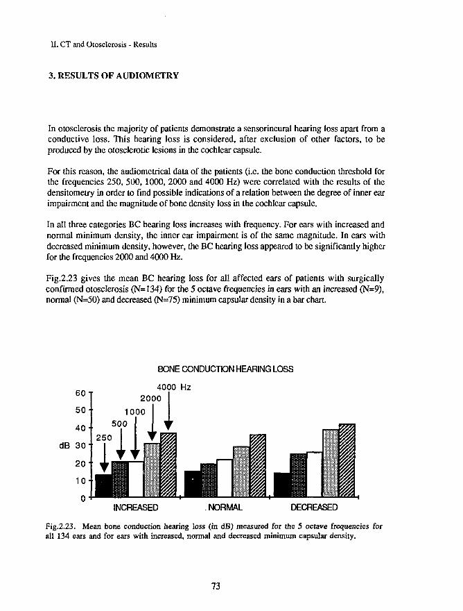
II. CT and Otosclerosis - Results
3. RESULTS OF AUDIOMETRY
In otosclerosis the majority of patients demonstrate a sensorineural hearing loss apart from aconductive loss. This hearing loss is considered, after exclusion of other factors, to beproduced by the otosclerotic lesions in the cochlear capsule.
For this reason, the audiometrical data of the patients (i.e. the bone conduction threshold forthe frequencies 250, 500, 1000, 2000 and 4000 Hz) were correlated with the results of thedensitometry in order to find possible indications of a relation between the degree of inner earimpairment and the magnitude of bone density loss in the cochlear capsule.
In all three categories BC hearing loss increases with frequency. For ears with increased andnormal minimum density, the inner ear impairment is of the same magnitude. In ears withdecreased minimum density, however, the BC hearing loss appeared to be significantly higherfor the frequencies 2000 and 4000 Hz.
Fig.2.23 gives the mean BC hearing loss for all affected ears of patients with surgicallyconfirmed otosclerosis (N=134) for the 5 octave frequencies in ears with an increased (N=9),normal (N=50) and decreased (N=75) minimum capsular density in a bar chart.
BONE CONDUCTDN HEARING LOSS
4000 Hz
INCREASED NORMAL DECREASED
Fig.2.23. Mean bone conduction hearing loss (in dB) measured for the 5 octave frequencies forall 134 ears and for ears with increased, normal and decreased minimum capsular density.
73

II. CT and Otosclerosis - Results
Fig.2.24 gives the BC threshold loss for ears with moderately (N=49) and severely (N=26)decreased minimum density. The mean loss at the frequencies 1000, 2000 and 4000 Hz issignificantly higher in ears with severely decreased minimum capsular density. These findingssuggest the presence of a relation between density loss and the degree of bone conductionhearing loss at the frequencies 2000 and 4000 Hz and possibly also at 1000 Hz.
BONE CONDUCTION HEARING LOSS
4000 Hz
MODERATELY DECREASED SEVERELY DECREASED
Fig.2.24. Mean bone conduction hearing loss for ears with a moderately and severely decreasedminimum density.
74

II. CT and Otosclerosis - Results
4. CORRELATION BETWEEN BONE DENSITY LOSS AND INNER EARIMPAIRMENT (BONE CONDUCTION HEARING LOSS)
In all 134 affected ears the bone density loss (i.e. minimum capsular density) has beencorrelated with the bone conduction threshold loss before surgery. As discussed above, boneconduction hearing loss in otosclerosis (after exclusion of other factors) is considered to resultfrom impairment of inner ear function by the otosclerotic focus in the bony cochlear capsule.We therefore investigated if a correlation exists between capsular density loss and boneconduction hearing loss for the various octave frequencies.
The following relations have been studied:
1. Maximum capsular density versus BC hearing loss2. Minimum capsular density versus BC hearing loss3. Density at predefined point 2-5 versus BC hearing loss
An analysis of simple linear regression was carried out and the correlation coefficients (R)were calculated. Correlation was considered:
"None1
'Low''Moderate'"High1
forforforfor
RRRR
<0.250.25 - 0.500.50 - 0.75
>0.75
R means IRI (in absolute values).Coefficients of the correlation between density (H) and bone conduction hearing loss were allnegative. This means that the correlations between density loss and bone conduction hearingloss were positive.
Correlations were calculated for all affected ears (§ 4.1), affected ears with increased (§ 4.2),normal (§ 4.3), and decreased (§ 4.4) minimum capsular density, and ears with moderately andseverely decreased minimum density (§ 4.5). Significant correlations are presented as positivevalues in the tables of the next paragraphs.
Significance was determined by means of the Student-t-test.Values of p > 0.05 were considered to be not significant. Between 0.01 and 0.05 a lowsignificance was accepted; a moderate significance between 0.001 and 0.01 and a highsignificance if p < 0.001.
A recapitulation of all correlations is given in paragraph 4.6.
75

•-L
II. CT and Otosclerosis - Results
4.1. ALL AFFECTED EARS (N=134)
In table 2.23 coefficients of the correlation between capsular density ar.d BC hearing loss atthe five octave frequencies are given for all affected ears. Only the significant (p<0.05)correlation coefficients are presented. The insignificant correlations are indicated by a dash.
250 500 1000 2000 4000 Hz
MaximumMinimum
Point 2Point 3Point 4Point 5
00
_
-
-.27.23
0.090.27
0.210.270.420.32
_
0.33
0.290.330.480.41
0.49
0.390.410.590.53
_
0.38
0.300.390.430.41
Table 2.23. Significant correlation coefficients between density value and BC hearing loss forthe five octave frequencies. An insignificant correlation is indicated by a dash (-).
Maximum densityNo significant correlations were found between maximum capsular density and BC hearingloss for the five octave frequencies except for 500 Hz. This correlation coefficient was verylow (R=0.09; p<0.05).
The absence of correlation was to be expected as maximum density in ears with otosclerosiswas found of the same magnitude and with about the same variation (SD = 75) as in normalears.
Minimum densityMinimum capsular density correlated significantly with BC-hearing loss at the five octavefrequencies except for 250 Hz. The strongest correlation was found with BC-hearing loss at2000 Hz. This correlation was highly significant (p<0.001).
Predefined pointsThe density at the predefined points correlated with BC hearing loss at the five frequenciesexcept for points 2 and 3 at 250 Hz. Correlation for all four points was maximal at 2000 Hz.
76

••I
n. CT and Otosclerosis - Results
4.2 AFFECTED EARS WITH INCREASED MINIMUM DENSITY (N=9)
No significant correlations were found between either maximum density, minimum density,or density at the four predefined points and bone conduction hearing loss in ears with anincreased minimum capsular density.
4.3 AFFECTED EARS WITH NORMAL MINIMUM DENSITY (N=50)
Only three correlations were significant between density and bone conduction hearing loss inthe ears with normal minimum density (table 2.24).
250 500 1000 2000 4000 Hz
Maximum - - . . .Minimum - - . . .
Point 2 . . . . .Point 3 . . . . o.31Point 4 . . . o.3O 0.29Point 5 -
Table 2.24. Significant correlation coefficients between density value and BC hearing loss forthe five octave frequencies. An insignificant corre'./iion is indicated by a dash (-).
Maximum densityNo significant correlation was found between maximum capsular density and BC hearing lossin ears with a minimum capsular density within the normal range (1674-1934 H).
Minimum densityMinimum capsular density (in the normal density range) did not correlate with BC hearingloss.
Predefined pointsA low correlation with low significance was found:
Between density at point 3 and BC-hearing loss at 4000 Hz: R=0.31; p<0.05Between density at point 4 and BC-hearing loss at 2000 Hz: R=0.30; p<0.05Between density at point 4 and BC-hearing loss at 4000 Hz: R=0.29; p<0.05
No other significant correlations were found.
77

' -L
H. CT and Otosclerosis - Results
4.4. AFFECTED EARS WITH DECREASED MINIMUM DENSITY (N=75)
Signiflcant correlations between density and bone conduction hearing loss in the ears withdecreased minimum capsular density are given in table 2.25.
250 500 1000 2000 4000 Hz
MaximumMinimum
Point 2Point 3Point 4Point 5
0
00
.24
_-
.39
.36
0.
0.0.0.
_
25
m
254636
_0.39
0.340.360.560.51
0.56
0.440.430.660.63
0.53
0.400.460.530.55
Table 2.25. Significant correlation coefficients between density value and BC hearing loss forthe five octave frequencies. An insignificant correlation is indicated by a dash (-).
Maximum densityMaximum capsular density showed no significant correlation with BC hearing loss.
Minimum densityMinimum capsular density, on the contrary, correlated significantly with BC hearing loss at1000 Hz (R=0.39; p<0.001),2000 Hz (R=0.56;p<0.001)and4000 Hz (R=0.53; p<0.001).Correlations with hearing loss at 250 Hz (R=0.24; p<0.05) and 500 Hz (R=0.25; p<0.05)were of low significance.
Predefined pointsDensity at the four predefined points correlated significantly with BC hearing loss except atthe lower frequencies (250, 500 Hz). Highest values of correlation coefficients were foundwith BC-hearing loss at 2000 Hz.
4.5. SUBGROUPS OF EARS WITH DECREASED MINIMUM DENSITY
In analysing the results it turned out that correlations within the group of ears with severelydecreased minimum density differed from those with moderately decreased minimum density.Since this difference may be important for the explanation of certain phenomena that are notwell understood both groups were analyzed in more detail.
78

. CT and Otosclerosis - Results
1. EARS WITH MODERATELY DECREASED MINIMUM DENSITY (N=49)
Significant correlations between density and bone conduction hearing loss in the ears withmoderately decreased minimum capsular density are given in table 2.26.
250 500 1000 2000 4000 Hz
MaximumMinimum
Point 2Point 3Point 4Point 5
0
000
_
.50
_
.63
.52
.38
0
00
.41
.45
.47-
0.71
0.590.800.48
0.77
.
0.600.830.47
0.73
.
0.900.650.52
Table 2.26. Significant correlation coefficients between density value and BC hearing loss forthe five octave frequencies. An insignificant correlation is indicated by a dash (-).
Maximum densityMaximum capsular density again showed no significant correlation with BC-hearing loss.
Minimum densityHighly significant correlations were present between minimum capsular density and boneconduction hearing loss at all five frequencies. The strongest correlations were found at thehigher frequencies:1000 Hz (R=0.71; p<0.001),2000 Hz (R=0.77; p<0.001) and4000 Hz (R=0.73; p<0.001).Correlation with 250 Hz (R=0.50; p<0.001) and 500 Hz (R=0.41; p<0.01) were lower butalso significant.
Predefined pointsDensity at the predefined points showed the following correlations with bone conductionhearing loss:
Point 2: no correlation.Point 3: moderate correlation with all frequencies and a high correlation at 4000 Hz (R=0.90;
p<0.001).Point 4: moderate to high correlations with a maximum at 2000 Hz (R=0.83; p<0.001) and
1000 Hz (R=0.80; p<0.001).Point 5: low to moderate correlations with a relative maximum at 4000 Hz (R=0.52;
p<0.001).
79

• -£
II. CT and Otosclerosis - Results
2. EARS WITH SEVERELY DECREASED MINIMUM DENSITY (N=26)
Significant correlations between density and bone conduction hearing loss in the ears withseverely decreased minimum capsular density are given in table 2.27.
250 500 1000 2000 4000 Hz
Maximum . . . . .Minimum - - - 0.60 0.57
Point 2Point 3Point 4 0.41 0.56 0.51 0.62 0.44Point 5 - 0.51 0.50 0.67 0.52
Table 2.27. Significant correlation coefficients between density value and BC hearing loss forthe five octave frequencies. An insignificant correlation is indicated by a dash (-).
Maximum densityAs for all other categories of ears, maximum capsular density did not correlate significantlywith bone conduction hearing loss.
Minimum densitySignificant correlations were only found with:2000 Hz (R=0.60; p<0.001) and4000 Hz (R=0.57; p<0.01).
Predefined pointsDensity at the predefined points showed the following correlations with bone conductionhearing loss:
Point 2: no correlationPoint 3: no correlationPoint 4: moderate correlations with a maximum at 2000 Hz (R=0.62; p=0.001).Point 5: moderate correlations with a maximum at 2000 Hz (R=0.67; p<0.001).
80

II. CT and Otosclerosis - Resulis
4.6. SUMMARY
Maximum density versus BC-hearing loss.
Maximum capsular density showed no significant correlations with BC-hearing loss either inthe total group of affected ears or in the subgroups with increased, normal or moderately andseverely decreased minimum density.
Minimum density versus BC-hearing loss.
Minimum density showed a low correlation with BC hearing loss in all frequencies except250 Hz in the total group of affected ears. No significant correlations were present in earswith increased and normal minimum density.In the ears with decreased minimum density the minimum showed a moderate correlation withBC-hearing loss at the high frequencies (2000,4000 Hz). In ears with a moderately decreasedminimum capsular density, higher correlations at all frequencies were found. In ears withseverely decreased minimum density, these correlations were lower and only significant at2000 Hz and 4000 Hz.
Density at point 2 versus BC-hearing loss
At point 2, situated in the ventro-medial wall of the basal cochlear turn, either no correlationsor only low ones were found. The relatively highest values were found at the frequencies1000,2000 and 4000 Hz (R=0.34,0.44 and 0.40 respectively).
Density at point 3 versus BC hearing loss
At point 3, located in the ventral wall of the basal cochlear turn, moderate to high correlationsappeared to be present for all frequencies in ears with moderately decreased minimum density.The highest correlation was found with 4000 Hz (R=0.90) and is presented in fig.2.27 as aregression line.
For ears with severely decreased minimum density, on the other hand, no significantcorrelations were found.
This difference is probably due to the much wider variation of the H-values at point 3 in earswith a severe decrease of minimum density (SD=419) as compared to those in ears with amoderate decrease (SD=104).
81

II. CT and Otosclerosis - Results
H 2000 -
1800 -
1600 -
10
Fig.2.25. Correlation between density at the predefined point 3 (Y-axis) and the BC hearingloss at 4000 Hz (X-axis) in 49 ears with a moderately decreased minimum capsular density.Correlation coefficient = - 0.90 (p<0.001).
Density at point 4 versus BC hearing loss
Density values at point 4, located in between the first and second cochlear turn on the ventralside of the cochlea, showed the highest correlations with BC-hearing loss for the frequencies1000 and 2000 Hz in ears with a moderately decreased minimum density (R=0.80 and 0.83).
Density at point 5 versus BC-loss
At point 5, located on the ventrolateral side of the second cochlear turn, the highestcorrelation with BC hearing loss was found in ears with a severely decreased minimumdensity (R=0.67) at 2000 Hz. All other correlation coefficients in both groups were of aboutthe same magnitude, except for BC loss at 500 Hz in ears with a moderate density loss.
82
II. CT and Otosclerosis - Conclusions
CONCLUSIONS
1. RADIODENSITY OF THE BONY COCHLEAR CAPSULE
Normal ears (N=35).
1. The radiodensity of the bony cochlear capsule was found to range from a mean minimumof 1804 H to a mean maximum of 2055 H. Spreading appeared to be small (SD: 65 and74 respectively).
2. Radiodensity was not correlated with age.3. Radiodensity of the cochlear capsule was homogeneous, at least in the ventral cochlear
wall. The density at the four predefined points ranged from 1884 H to 1925 H with aboutthe same standard deviations as for the maximum and minimum density.
Otosclerosis (affected ears: N=134; non-affected ears: N=13)
1. On visual examination areas of density loss in the labyrinthine capsule were found in19% (N=16) of the patients with otosclerosis (N=84). In 15% (N=13) these foci werebilaterally present, in 4% (N=3) unilaterally. In 81% no radiolucent foci were seen.
2. Wilh densitometry, density loss (minimum density below of that in control ears minus2.SD) was found in 56% (N=75) of the affected ears (N=134).
3. In 19% (N=26) of the affected ears, density loss was severe (<1500 H). In all these ears,except one, radiolucent areas were found on visual examination.
4. In 37% (N=49) density loss was moderate (1500-1674 H). In ihese ears no radiolucencieswere discovered by the naked eye except for two cases.
5. From these results it may be concluded that- Only foci with a minimum density below 1500 H are visible with the naked eye- Densitometry is a far superior method to detect foci with density loss.
6. In ears affected by otosclerosis the minimum density value in the cochlear capsule wasfound to increase slightly with age.
7. No difference in density loss was found between the four predefined points in the ventralwall of the cochlear capsule. A predelection place of the otosclerotic focus could not beestablished in the ventral cochlear wall.
8. In ears affected by otosclerosis, maximum density was not found to be increased. A healedfocus does not seem to have a higher radiodensity than the normal bone of the cochlearcapsule.
9. In ears of patients with otosclerosis that were not (yet) clinically affected, both theminimum and maximum radiodensity were within the normal range.
84

--L
H. CT and Otosclerosis - Conclusions
2. CORRELATION BETWEEN BONE DENSITY LOSS AND BC-HEARINGLOSS
1. Bone conduction hearing loss appeared to increase with the degree of bone density loss inthe cochlear capsule.
2. Maximum capsular density was not correlated with BC hearing loss.3. Minimum capsular density was correlated with BC hearing loss when this minimum is
decreased:a. In ears with moderately decreased minimum density, high correlations existed with BCloss at the higher frequencies (1000, 2000 and 4000 Hz) and moderate correlations withhearing loss at the lower frequencies (250 and 500 Hz).b. In ears with severely decreased minimum density, correlations were moderate at 2000and 4000 Hz and low or absent at other frequencies.
4. Density loss at:Point 2 (located on the ventro-medial side of the first cochlear turn) had a lowcorrelation with BC hearing loss at the higher frequencies in all affected ears. In the twosubgroups (moderately and severely decreased minimum density) correlations weie notsignificant.Point 3 (located on the ventral side of the first cochlear turn) was moderately correlatedwith BC hearing loss at all frequencies and highly correlated with BC hearing loss at 4000Hz in ears with moderately decreased minimum density. In ears with severely decreasedminimum density, correlations were not significant.Point 4 (located between the first and second cochlear turn) was highly correlated withBC hearing loss at 1000 and 2000 Hz in ears with moderately decreased minimumdensity. Correlations with the other frequencies were low or moderate. In ears withseverely decreased minimum density these correlations with BC hearing loss weremoderate at 500,1000 and 2000 Hz and low at 250 and 4000 Hz.Point 5 (located on the ventral side of the second cochlear turn) showed low to moderatecorrelation coefficients with BC hearing loss at all frequencies in ears with moderately andseverely decreased minimum density. The relatively highest correlations were found withBC hearing loss at 2000 Hz.
3. TOPOGRAPHICAL CORRELATIONbetween the location of bone density loss and BC hearing loss for thevarious frequencies.
From the data summarized above in conclusion 2.4 it appears that density loss in thebasal cochlear turn (point 3) correlates best with BC loss at high frequencies whereasdensity loss between the first and second cochlear turn (point 4) correlates best with BCloss at middle frequencies. This finding points to a possible topographical relationbetween the location of density loss in the cochlear capsule and the location of hearingperception within the cochlea.
85

II. CT and Otosclerosis - Discussion
DISCUSSION
Otoradiological planes.
In our study we have come to the conclusion that the transverse plane (Hirtz) is the plane offirst choice in studying labyrinthine otosclerosis. Both temporal bones are depicted at thesame time, which gives the opportunity to make corrections in the patients' positioningduring the examination in a simple way.It is a comfortable plane in the patients' positioning as compared to its equivalent in classicalpolytomography. All other planes as described in part 1 of this study are perpendicular to thetransverse plane.Other CT studies (Swartz et al, 1984; Mafee et al, 1985a,b) made use of this plane as well.
As the second plane of investigation, in addition to the transverse plane, we preferred thesemi-longitudinal plane (Zonneveld) for direct scanning of the cochlear capsule. It enables acomplete visualization of the basal cochlear turn. This plane appeared to be of greatimportance in the densitometrical study in order to establish the value of maximum andminimum capsular density.The semi-axial (Guillen) and axio-petrosal (Poschl) planes are more perpendicular to thestapedial footplate and therefore give a better imaging of the oval window region. This makesthese planes preferable in the examination of cases with 'fenestral' otosclerosis.For investigation of 'fenestral' otosclerosis and the position of a stapes prosthesis, thetransverse plane can thus best be combined with the semi-axial or axio-petrosal plane. Ininvestigating 'labyrinthine' otosclerosis the transverse and the semi-longitudinal planes arepreferable.
Density of the normal bony cochlear capsule and its relation to age.
The petrous bone, and especially the labyrinthine capsule is the most dense bone in thehuman body. In our study the radiodensity of the normal cochlear capsule was found to rangefrom about 1800 H to 2050 H. The three different layers of bone which compose thelabyrinthine capsule (periostal, middle and endoslal layer) as described by Anson (1973) couldnot be discerned by means of our technique nor in other CT studies (Mafee et al, 1985a).Possible remnants of primary (fetal) cartilage within the middle layer of the capsule could notbe visualized.Capsular density normally has very little variation. The entire capsule is relatively isodensand has a regular aspect on CT.The bony labyrinthine capsule remains relatively inert and unchanged throughout life(Shambaugh & Glasscock, 1980). In our normal control ears, no correlation was foundbetween capsular density and age. A post-mortem densitometrical study of normal petrousbones by Krmpotic-Nemanic et al (1976) suggested that demineralization of the labyrinthinecapsule takes place with aging. This could not be confirmed by our densitometric study:neither the maximum capsular density nor the minimum capsular density was correlated withage of the control subjects.
86

II. CT and Otosclerosis - Discussion
Visualization of spongiotic and sclerotic foci
In otosclerosis the dense 'ivory-like1 endochondral bone is partially replaced by spongiotic,highly vascularized foci of haversian bone tissue (otospongiosis). These foci may becomeremineralized again after some time (otosclerosis).
Sclerosis and spongiosis are considered to represent two stages of the same disease by themajority of authors. A sclerotic lesion is considered to be the late and healed stage of aremineralized spongiotic lesion (Shambaugh: 1965,1966,1969; Riiedi: 1965, 1969; Nager,1969). 'Lyric' and 'rebuilding' phases, however, may occur simultaneously in one focus(Bretlau et al, 1982). According to some authors (Parahy & Linthicum, 1984), theotospongiotic stage does not necessarily precede the sclerotic stage.
Radiolucent areas in the labyrinthine capsule could be imaged in various polytomographicalstudies (Derlacki & Valvassori, 1965; Hoople & Basch, 1966; Valvassori, 1966,1969,1973;Valvassori & Naunton, 1967; Applebaum & Shambaugh, 1978) . Recently they were studiedby means of CT by our group (Damsma et al, 1984; Zonneveld et al, 1984; De Groot et al,1985) and by Mafee et al (1985a) and Swartz et al (1985a,b). In our study we were unable todiscern between hypermineralized otosclerotic foci and normal capsular bone; this is incontrast to Mafee et al (1985a) who distinguished between sclerotic, spongiotic and mixedchanges. As the sclerotic lesions are adjacent to normal bone (Parahy & Linthicum, 1984),they can only be detected by an irregularity of the outlining of the labyrinthine lumen. Sincepartial volume effects strongly interfere with the sharpness of transition zones, we wereunable to prove that these delicate irregularities were caused by the presence of sclerotic foci.Since spongiotic lesions were found to be irregular in shape and size, the presence of sclerosisat the border of these lesions adjacent to normal capsular bone could not be established for thesame reason.
Percentage of radiolucencies detected
In this study about 20% of the affected ears of patients with surgically confirmed otosclerosisshowed areas of demineralization in the labyrinthine capsule. In former polytomographicalstudies these percentages varied extremely and in some studies no radiolucencies were found atall. Most of these studies are characterized by a lack of homogeneity of the material (patientsc.q. ears) and by inconsistent radiographical methods. In the CT studies of Swartz et al (1984)and Balli et al (1986), fenestral otosclerosis was investigated so that no comparison with ourinvestigation can be made. Mafee et al (1985a) selected patients on the basis cf abnormallabyrinthine capsules in CT scans. Due to this selection method our data cannot be comparedwith those of the latter study.
In our study, in about 80% of the affected ears no visible areas of density loss were found.Non-visibility of foci can be caused by:
87
II. CT and Otosclerosis - Discussion
a. The size of the spots. If a focus is smaller than the spatial resolution of the CT scanner itwill not be visible.b. The amount of density loss within a focus. The difference in radiodensity between a focusand the surrounding normal bone should exceed a certain value in order to be visible by thenaked eye. According to our study this difference should be more than 500 H with the windowsetting which is normally used in temporal bone scanning.
Oensitometrically the presence of such small foci is plausible as in 37% of the affected ears a(moderately) decreased minimum capsular density was present without visible foci of densityloss.
Location and extension of the lesions
Although these otosclerotic lesions may originate in almost every part of the labyrinthinecapsule, predelection areas have been described (Nager, 1969; Shambaugh & Glasscock,1980). The fissula ante fenestram, the region just anterior to the oval window niche and theborder of the round window niche, are considered such predelection areas (Bretlau, 1969). Thepathological process is considered to begin at these sites in 90% of the cases.
In our visual study we found areas of density loss throughout the entire labyrinthine capsule.In some cases one large confluent lesion wrapped around the labyrinth was present, leavingthe thin endostal bone layer intact. These we named 'ring type' lesions. In other cases thelesion was irregular in shape and size, invading the endostal bone layer and extending to theoutline of the endolabyrinthine lumen. These we called 'patchy* lesions. We never captured avisual image of a protrusion of a focus into the lumen. In our patients the classicalpredelection areas were always involved.
However, isolated small and beginning lesions in the oval and round window niche can easilybe missed because of the interference of partial volume averaging effects if foci are adjacent tothe middle ear cavity. This may (partially) account for the low percentage of foci found and forthe fact that the presence of predelection places at the cochlear base could not be confirmed.
In our study no difference in the density of the four predefined points at the basal coil, middlecoil and apical area of the ventral cochlear wall was measured. This suggests that in advancedotosclerosis no systematic difference in degree of demineralization exists, at least not in theventral cochlear wall.
Remineralized foci
A large variation of minimum capsular density was found in the affected ears. Values variedfrom "severely decreased' to 'increased1. Demineralized 'spongiotic1 lesions were visible in thecochlear capsules with the lowest H values (<1500 H) of minimum density. In ears with a
88

II. CT and Otosclerosis - Discussion
'moderately decreased' minimum density the cochlear capsule generally had a normal, smoothaspect on visual evaluation. In this group of ears the highest correlation was found betweenbone conduction hearing loss and density values. It could be possible that in these earssclerotic foci (with a density lower than that of normal capsular bone and higher than that of'dcmineralizcd' foci) are solely responsible for the moderate decrease in minimum densitywhich is invisible by examination with the naked eye.
Foci in non-affected ears
It is generally accepted that otosclerosis is clinically unilateral in about 10-15% of thepatients. In our study 15 out of 89 patients had unilateral symptoms i.e. 17%. It is oftenassumed that otosclerosis in these cases is histologically bilateral but that symptoms haveoccurred in one ear only.
In none of the non-affected ears of our patients, however, radiodensity loss was found bymeans of densitometry. This finding suggests that clinically unilateral otosclerosis is reallyunilateral indeed; this needs to be histologically confirmed.
Positive correlation between BC threshold loss and bone density loss.
In our study a positive correlation was found between BC-threshold loss and minimumcapsular density. It appears that the magnitude of BC loss increases with the degree of bonedensity loss and that hearing is most impaired in ears with evidence of otospongiosis. Thisfinding corroborates the hypothesis that the bone lesion is directly 'responsible' for thesensorineural hearing impairment that is present in a great number of otosclerosis patients.
Our results do not allow a conclusion as to the pathogenesis of the impairment of cochlearfunction. This could be the result of toxic-enzymatic processes as was claimed by Brctlau et al(1971, 1982) and Chevance et al (1970,1972). It is unlikely that the effect is mechanical anddue to ingrowth of (he otosclerotic lesion into the spiral ligament and/or cochlear lumen. Thiscould not be radiologically confirmed in our patients.That otospongiotic lesions could affect cochlear function through impairment of itsvascularization (in particular venous drainage), as has been claimed by Riiedi (1965, 1969),can neither be ruled out nor confirmed.
According to Parahy & Linthicum (1984) spongiotic lesions adjacent to the spiral ligamentproduce a much greater amount of hyalinization than sclerotic lesions and this hyalinizationshould be responsible for the degree of bone conduction hearing loss. Therefore, spongioticfoci would produce more inner ear hearing loss than sclerotic foci. In our study, ears withseverely decreased minimum density (i.e. ears with spongiotic lesions within the cochlearcapsule) showed the most severe BC hearing loss. This agrees with the histological findingsof Parahy & Linthicum.
89

II. CT and Otosclerosis - Discussion
Topographical correlation between location of bone density loss and BChearing loss for the various frequencies.
In the total group of affected ears, the highest correlations between bone density loss and boneconduction hearing loss were found for points 4 and 5 with 1000, 2000 and 4000 Hz. Thecorrelation coefficients between all other points and frequencies were below 0.50.In the group of ears with visible density loss ('severely decreased minimum density1) the samecorrelations were found and, in addition, point 4 and 5 were found to correlate with BChearing loss at 500 Hz.
In the group of ears without visible density loss but with moderately decreased minimumdensity the highest correlations were measured with BC hearing loss. Highest R-values werefound: between point 3 and 4000 Hz (R=0.90) and between point 4 and 2000 Hz and 1000 Hz(R=0.83 and R=0.80). This means that density loss at a point near the basal cochiear turn(point 3) correlates best wilh BC hearing loss at a high frequency (4000 Hz) and that densityloss at a point close to the second cochiear turn (point 4) correlates best with BC loss atmiddle frequencies (1000 and 2000 Hz). This finding is approximately in agreement with thelocation of frequency perception in the cochiear turn.
We do realize that this method needs refinements (e.g. by using more predefined measuringpoints) to be able to prove wilh more certainly the existence of a topographical correlationbetween density loss at certain points in the cochiear capsule and inner ear impairment forcorresponding frequencies.
We think to have developed a sensitive method to establish the degree of demineralizalion inthe labyrinthine capsule of patients with otosclerosis. This method could be used for thefollow-up of patients treated with sodium fluoride in a prospective study.
90

II. CT and Otosclerosis - References
REFERENCES OF PART II
1. Anson BJ, Donaldson JASurgical anatomy of the temporal bone and ear.Saunders, Philadelphia (2nd ed.): 1973
2. Applebaum EL, Shambaugh GE JrOtospongiosis (otosclerosis): Polytomographic and histologie correlation.Laryngoscope 88:1761-1778,1978
3. Balli R, Canossi GC, Torricelli PImpiego della tomografia computerizzata ad alta risoluzione nello studio dcH'otosclerosi.Audiol.Ital. 3:25-30,1986
4. Bretlau PRelation of the otosclerotic focus to the fissula ante f enestramJ. Laryngol. Otol. 83:1185-1193,1969
5. Bretlau P, Causse J, J0rgensen MB, Chevance LGHistiocytic activity in otosclerotic bone.Arch. Ohr-Nas.-Kehlkopfheilk. 198: 301,1971
6. Br-jUau P, Chevance LG, Causse J, J0rgensen MBBone résorption in otospongiosis.Am Journal of Otol Vol.3, Nr 3:284-289,1982
7. Britton BH, Linthicum FHOtosclerosis: Histologie confirmation of radiologie findings.Ann Otol Rhinol Laryngol 79: 5-11,1970
8. Carhart RCochlear otosclerosis: Audiological considerationsAnn Otol Rhinol Laryngol 75: 559,1966
9. Chevance LG, Bretlau P, J0rgensen MB, Causse JOtosclerosis. An electron microscopic and cytochemical study.Acta Otolaryngol Suppl. 272,1970
10. Chevance LG, Causse J, Bretlau P, J0rgensen MB, Berges JHydrolytic activity of the perilymph in otosclerosis.Acta Otolaryngol 74:23,1972
11. Compère WERadiologie findings in otosclerosis.Arch. Ololaryngol. 71:150-155,1960
12. Compère WERadiologie findings in patients with otosclerosis.J Laryngol. 78: 649-653,1964
13. Damsma H, De Groot JAM, Zonneveld FW, Van Waes PFGM, Huizing EHCT of cochlear otosclerosis (otospongiosis).Radiol Clin North Am 22 (I): 37-43,1984
14. De Groot JAM, Huizing EH, Damsma H, Zonneveld FW, Van Waes PFGMLabyrinthine otosclerosis studied by means of a new computed tomography technique.Ann Otol Rhinol Laryngol 94 (3): 223-225,1985
15. Derlacki EL, Valvassori GEClinical and radiological diagnosis of labyrinthine otosclerosis.Laryngoscope 75:1293-1306, 1965
91

H. CT and Otosclerosis - References
16. Engström HUeber das Vorkommen der Otosklerose nebst experimentellen Studien über chirurgischeBehandlung der KrankheitActa Otolaryngol Suppl. 43, 1940
17. Freeman JProgressive scnsorineural hearing loss and cochlear otosclerosis: a prospective study.Laryngoscope 89:1487-1521,1979
18. Guild SHistologie otosclerosisAnn Otol Rhinol Laryngol 53: 246,1944
19. Hoople GD, Basch RIRadiographie findings in cochiear otosclerosis.Ann Otol Rhinol Laryngol 75: 688-697,1966
20. Krmpotic-Nemanic J, Nemanic G, Simunic V, Miklic P, Favesic Z,Ivankovlc D Aequidensitometrie der Labyrinthkapsel mit besonderer Rücksicht desBodens des inneren Gehörganges.G. Thieme Verlag (Stuttgart): Laryng. Rhinol. 55: 682-686,1976
21. Lintbicum FH, Forquer BDSodium fluoride as a treatment for otosclerotic hearing loss.Am Journal of Otol 6/1: 35-37,1985
22. Mafee MF, Valvassori GE, Deitch RL, Norouzi P, Hendrikson GC, et alUse of CT in the evaluation of cochlear otosclerosis.Radiology 1985; 156: 703-708
23. Mafee MF, Hendrikson GC, Deitch RL, Norouzi P, Kumar A, Kriz R,Valvassori GEUse of CT in stapedial otosclerosis.Radiology 1985; 156:709-714
24. Nager GTHistopalhology of otoscerosis.Arch. Otolaryngol. 89:341-363,1969
25. Nylen BHistopathological investigations on the localization, number, activity and extent ofotosclerotic foci.J Laryng 63: 321,1949
26. Parahy Chr, Lintbicum FH,Otosclerosis and otospongiosis: Clinical and histological comparisons.Laryngoscope 94/4: 508-512,1984
27. Politzer AUeber primäre Erkrankung der knöchernen Labyrinthkapsel.Z. Ohrenheilk. 25: 309,1894
28. Rovsing HFundamentals of Ear tomography; Otosclerosis.Charles Thomas Publishers, Springfield Illinois: 164-178,1971
29. Ruedi L, Spoendlin HDie Histologie der otosklerotischen Stapesankylose im Hinblick auf die chirurgischeMobilisation des Steigbügels.Bibl. oto-rhino-laryng. Fase. 4:1,1957
30. Rüedl LHistopathologic confirmation of labyrinthine otosclerosis.Laryngoscope 75:1582-1610,1965
92
II. CT and Otosclerosis - References
31. Rtiedi LOtosclerotic lesions and cochlear degeneration.Arch Otolaryng 89:180-187, 1969
32. Schuknecht HF, Gross COtosclerosis and the inner ear.Ann Otol Rhinol Laryngol 75: 423,1966
33. Schuknecht HF, Kirchner CJCochlear otosclerosis: fact or fantasy.Laryngoscope 84:766-782,1974
34. Schuknecht HFThe pathology of the ear.Harvard University Press, Boston: 351-388,1976
35. Shambaugh GEClinical diagnosis of cochlear (labyrinthine) otosclerosis.Laryngoscope 75: 1558-1562,1965
36. Shambaugh GEThe therapy of cochlear otosclerosis.Ann Otol Rhinol Laryngol 75: 579-583,1966
37. Shambaugh GESodium Fluoride for inactivation of the otosclerotic lesion.Arch. Otolaryngol. 89: 381-382,1969
38. Shambaugh GE, Glasscock MESurgery of the earSaunders, Philadelphia (3d ed.): 445-475, 1980
39. Siebenmann FTotaler knochemer Verschluss beider Labyrinthfenster und Labyrinthitis serosa infolgeprogressiver Spongiosierung.Verh Dtsch Otol Ges: 267-274,1911
40. Swartz JD, Faerber EN, Wolfson RJ, Marlowe FIFenestral otosclerosis: Significance of preoperative CT evaluation.Radiology 151:703-707,1984
41. Swartz JD, Mandell DW, Berman SE, et atCochlear otosclerosis (otospongiosis): CT analysis with audiomctric correlationRadiology 155:147-150,1985
42. Swartz JD, Mandell DW, Wolfson RJ et alFenestral and cochlear otosclerosis: CT evaluationAm J Otology 6 (6): 476-481,1985
43. Valvassori GEradiological diagnosis of cochlear otosclerosis.Laryngoscope 75:1563-1571,1965
44. VaWassoriGEThe : 'terpretation of the radiographic findings in cochlear otosclerosis.Arm Otol Rhinol Laryngol 75: 572-578,1966
45. Val- ssori GE, Naunton RFDiagnostic correlates in fenestral otosclerosis.Laryngoscope 77:734-743,1967
46. Valvassori GETomographic findings in cochlear otosclerosis.Arch Otolaryng 89:193-196,1969
93

II. CT and Otosclerosis - References
47. Valvassori GEOtosclerosis.Otolaryngol Clin North Am 6:379-389,1973
48. Valvassori GE, DobbenCT densitomelry of the cochlear capsule in otosclerosis.Am. J. Neuroradiology 6: 661-667, 1985
49. Vignaud JFundamentals of Ear Tomography: OtosclerosisCharles Thomas Publishers, Springfield Illinois 153-163,1971
50. VirolainenVestibular disturbances in clinical otosclerosis.Acta Otolaryngol Suppl. 306,1972
51. Zonneveld FW, De Groot JAM, Damsma H, Van Waes PFUM, Huizing EHDie Anwendbarkeit der hochaufldsenden CT zur Darstellung des Aquaeductus Vestibuli(Meniere) und der Otospongiosis des Labyrinths.Radiologie 24: 508-515,1984
94

COMPUTED TOMOGRAPHY
INVESTIGATION
OF THE
VESTIBULAR AQUEDUCT
IN
MENIERE'S DISEASE

I. CT of the temporal bone
CONTENTS OF PART III
1. GENERAL CHARACTERISTICS OF MENIERE'S DISEASE 971.1. Definition and incidence 971.2. History 971.3. Clinical aspects 971.4. Pathogenesis 98
2. PATHOPHYSIOLOGY 99
3. ANATOMY OF THE VESTIBULAR AQUEDUCT 101
4. VISUALIZATION OF THE VESTIBULAR AQUEDUCT 103
Literature study
5. OBJECTIVES OF THE PRESENT STUDY 109
6. MATERIALS... 1106.1. Selection criteria 1106.2. Patients and ears I l l6.3. Normal ears used as controls 112
7. METHODS 1147.1. Planes of CT examination 1147.2. Visibility scale of the vestibular aqueduct 1147.3. Visual evaluation of the CT scans 1167.4. Measuring the length of the vestibular aqueduct 1177.5. Audiometry 118
8. RESULTS 1208.1. Visibility of the vestibular aqueduct 1208.2. Length of the vestibular aqueduct 122
9. CONCLUSIONS 125
10. DISCUSSION 126
11. REFERENCES 132
96

III. CT and Meniere's disease - Introduction
GENERAL CHARACTERISTICS OF MENIERE'S DISEASE
Definition and incidence
Meniere's disease is a labyrinthine disorder of unknown origin with a triad of symptoms:deafness, tinnitus and vertigo spells. The name 'Menidre's disease' is preferable to 'Meniere'ssyndrome' or 'Meniere's symptom-complex1 because the latter two terms suggest that thecondition is a complex of symptoms without a known pathological substrate. On thecontrary, the clinical features of the condition are so clearly defined that it is allowed to speakof it as a disease.
The incidence of the disease in die Caucasian race as given in the literature varies from 0.05%to 0.16%. This variation is partially due to differences of opinion as to die definition of thedisorder. The term 'Meniere's disease' is, in some instances, applied to all patients withcomplaints of paroxysmal vertigo whereas others reserve it for a well-defined condition.Consequently, the clinical syndrome that one clinician considers to be a real case of Meniere'sdisease may not be so considered by another clinician (Pfaltz, 1986).
Meniere's disease is more predominant in the Caucasian race. It has its highest incidence in theage groups 30 to 50 years and is rare in children and the elderly. It is somewhat more frequentin females than in males. Meniere's disease usually affects one ear. It becomes bilateral inabout one quarter of the cases but also in this respect the percentage varies widely in theliterature.
History
In 1861 Prosper Meniere (1799-1862) for the first time described the classic combinationof deafness, tinnitus and vertigo that has since become known as 'Maladie de Meniere'(Meniere, 1861; Tarle, 1961). His description was so accurate that, ever since, no additionswere needed. In short, he described a condition characterized by sudden and repeated spells ofvertigo, often accompanied by nausea and vomitus, tinnitus and hearing impairment, withnormal hearing before the onset of the disease and without symptoms between the dizzyspells.
Clinical aspects
Hearing loss is of the sensorineural type and characterized by loudness recruitment, decreasedspeech discrimination and normal perstimulatory adaptation. In the beginning, hearing lossfluctuates, especially in the lower frequencies. Hearing may vary with the vertigo attacks. It
97

III. CT and Meniere's disease - Introduction
may decrease in combination with the vertigo spell or improve after the attack. In the courseof the disease the hearing threshold curve flattens and hearing loss becomes irreversible.
Tinnitus may vary from a pure tone sensation to a combination of whistling, buzzing androaring. After the attack its intensity mostly decreases and it may even disappear in between.In later stages tinnitus is constantly present in most instances.
The vertigo attacks are frequently preceded by a sensation of fullness or pressure in the ear.Onset is frequently sudden with a maximum of symptoms within a few minutes. Thesymptoms may last for some hours and can disappear completely afterwards. Thesymptomatology of Meniere's disease may vary to the extent that some patients have all threesymptoms at the same time from the onset of the disease, whereas others suffer in thebeginning from hearing loss and tinnitus (cochlear type) or vestibular symptoms only(vestibular type). Attacks, associated in the beginning of the disease with nausea and vomitus,can occur at any time and at any place, even during sleep. Neurologic symptoms are normallylacking.
Typical psychological characteristics have been attributed to "the Meniere's patient': hardworking, overconscientious and suggestible. Attacks may sometimes be evoked by stress orfatigue.
Pathogenesis
From the symptomatological and histopathological data in man and in animal experiments(Kimura and Schuknecht, 1985; Kimura, 1968), (he pathogenesis of Meniere's disease is mostlikely as follows: due to atrophy of the resorptive epithelium in the endolymphatic sac andduct of unknown origin, a hydrops of the endolymphatic system gradually develops.Reissncr's membrane, sacculus and utriculus are distorded and their electrolyte and fluid barrierfunction becomes impaired. Leakage and membrane ruptures occur, leading to attacks and/ormore or less fluctuating symptoms of hearing loss, tinnitus and vertigo. Due to mechanicaland toxic factors, the hair cells, nerve fibers and ganglion cells ultimately degenerate. Untilnow, however, it has not been proven that endolymphatic hydrops in man causes thesymptoms in Meniere's disease (Plantenga, 1983).
98

HI. CT and Meniere's disease - Pathophysiology
PATHOPHYSIOLOGY OF MENIERE'S DISEASE
Inner ear fluids
The formation, pattern of circulation and turnover of the inner ear fluids are not yet clearlyunderstood. Perilymph originates from plasma without substantial electrolyte exchange.Endolymph is mainly derived from perilymph. The stria vascularis is believed to play animportant role in its ultimate fluid and electrolyte composition. The Na+ and K+
concentration in the endolymph is similar to that of intracellular fluid compartments; the striavascularis is considered to maintain the required gradients between perilymph and endolymph.In the endolymphatic sac, protein concentration is much higher than in the scala media. Innerear fluids are thought to have a function in the transport of oxygen and nutrients to thecellular elements as well as in the removal of metabolic waste products. Perilymph andendolymph maintain a hydrostatic equilibrium and provide the required ionic environment forlabyrinthine biopotentials. Furthermore, they serve as a medium for the transmission ofvibrations from the stapedial footplate to the basilar membrane of the organ of Corti and as astimulus mediator in the vestibule and the cupula of the semicircular canals.
Regulation of inner ear fluid composition
Electrolytes in the inner ear fluid (e.g. sodium, potassium, chloride) are transported by passivediffusion (electrochemical gradient) as well as by active transcellular ion exchange withpassive outflow of water through the surrounding epithelium. An active transcellular vacuolarendolymph outflow has been postulated as well (Fribcrg, 1985). These active mechanismsmake use of enzymes e.g. Na-K-ATPase (Juhn et al, 1987). Prostaglandin may be involved inthe maintenance of a stable membrane permeability to water and ions through enzymes likeadenylate cyclase and cyclic adenosine monophosphaiase.Maintenance of a positive endocochlear potential and endolymphatic ion concentration,necessary for an adequate labyrinthine function, is a complex mechanism that, still today, isnot clearly understood.Another mechanism in the regulation of the inner ear fluid composition is the blood-labyrinthbarrier (Juhn et al, 1985). This is a barrier for large molecular weight substances. Althoughsmall molecular weight substances (e.g. glucose) can pass from the bloodserum into theperilymph, inhibition of entry occurs at a certain saturation of the perilymph, which indicatesthat this transport is carrier-mediated. In this way the blood-labyrinth barrier works as aprotecting mechanism for the stability of the inner ear fluids.
Pathogenesis of endolymphatic hydrops
The cause of endolymphatic hydrops is not known. Several mechanisms have been speculated.1. From animal experimental work (in guinea pigs) it is known that destruction of theendolymphatic sac causes endolymphatic hydrops.2. Metabolic or allergic factors may cause a change in osmotic pressure of the inner ear fluids,
99

HI. CT and Meniere's disease - Pathophysiology
causing hydrops that subsequently mechanically destroys the perilymph-endolymph barrier(e.g. Reissner's membrane), resulting in a "diffuse membrane leakage'. Disturbance of themembrane permeability may be induced by an increase of prostaglandin-synlhesis provoked byacute stress stimuli (Juhn et al, 1987).
Since the early hydrops hypothesis of G.Portmann (1919), many experiments in differentanimals have been carried out in order to study the histological changes in the labyrinthinestructures under these experimental conditions (Kimura & Schuknecht, 1965; Kimura, 1968).An experimental hydrops starts in the basal coil within a few weeks and progresses to allcochlear turns within one month after cndolymphatic duct or sac obliteration. Reissner'smembrane becomes distended and connected to the bony wall and shows a variety ofdegenerative alterations (Ruding et al, 1987). Hair cell loss commences apically (Arenberg etal, 1970, 1976a; Albers et al, 1987a). In the beginning only the outer hair cells are affectedand the stria vascularis shows a variety of degenerative changes (Albers et al, 1987b).
Three possible mechanisms are postulated to cause hydrops after destruction of theendolymphatic sac (see Pfaltz, 1986):
1. The stria vascularis secretes the endolymph that flows through the cndolymphatic duct tothe endolymphalic sac where reabsorption and phagocytosis of cell-debris takes place. Anydisturbance in this 'longitudinal endolymph flow' may cause a relative hypertension in theendolympatic system. Such a disturbance may be due to malabsorption in the endolymphaticsac or to a mechanical obstruction anywhere in the endolymphatic duct.
2. Due to the absence of phagocytosis, an accumulation of cell debris occurs in theendolymph which leads to an increased colloid osmotic pressure and consequently to ahydrops.
3. A third postulate is that a change in osmolarity takes place by a shift of ion concentrationin the cochlear endolymph. The increased difference of osmotic pressure between theendolymph and the surrounding tissue is the driving force for the water movement Even animbalance of 0.1 mOsm can cause a dilatation of the endolymphatic space.
Impairment of saccus endolymphaticus function
Several authors have found an atrophy of the saccular epithelium (see: Pfaltz, 1986).Disturbances in the saccus itself may be caused by perisaccular fibrosis resulting in animpairment of the blood supply of the endolymphatic duct and sac (Hallpike & Cairns, 1938;Altmann & Zechner, 1968; Shambaugh, 1968). Bony obstructions of the vestibular aqueducthave been initially described (Clemis and Valvassori, 1968) in a tomographic study in 1968.A relation exists between pneumatization of the mastoid and the width of the vestibularaqueduct (Wilbrand, 1976, 1980; Wilbrand et al, 1974, 1978). Recurrent otitis media issupposed to play a role in it (Oigaard et al, 1975).
100

HI. CT and Mcniere's disease - Anatomy
ANATOMY OF THE VESTIBULAR AQUEDUCT
The vestibular aqueduct is a bony canal in the labyrinthine capsule extending from the medialwall of the vestibule to the dorsal surface of the petrous bone. In this canal the membranousendolymphatic duct connects the utricle-saccule complex with the endolymphatic sac that islocated in the subarachnoidal space of the posterior cranial fossa.
In the fetal period the vestibular aqueduct is formed around a pre-existent part of themembranous labyrinth, the endolymphatic duct, whose epithelium is continuous with that ofthe utricle and saccule (Anson, 1965; Anson et al, 1968). Initially the vestibular aqueduct isstretched and runs parallel to the common cms of the semicircular canals. During further fetaldevelopement the route of the vestibular aqueduct undergoes a change resulting in a morecaudal location of the distal part, whereas the proximal part remains parallel to the commoncms. The result is a bended course with its "knee1 directed cranially.
In adults the total length of the vestibular aqueduct is approximately ten millimeters (Anson,1965). It is divided into two parts:
1. The proximal part or 'isthmus' with a length of 1.5 mm and a mean diameter of 0.35 mm(range: 0.25 to 0.50 mm).2. The distal part with a triangular shape whose smallest diameter is at the transition to theisthmus (0.5 mm.). The aperture contains a part of the endolymphatic sac and has an averagewidth of 3.2 mm (range: 0.65 - 4.55 mm). Cross sections of this part show ovoid shapeswith the largest diameter in the horizontal plane and a torsion in its course, resulting in aflattened fissure rather than a circular pore. The normal shape and course of the aqueduct andits relation to the labyrinth are presented in the four drawings of figs. 3.1 - 3.4.
The angle of the course of the vestibular aqueduct has been measured by Wilbrand et al (1974)and Sando & Ikeda (1984) and was found to vary from 90 to 135 degrees. There is a negativecorrelation between the length of the aqueduct and the angle in such a way that the shorter theaqueduct, the wider the angle. Caudotropic forces during the post-midterm growth exerted onthe endolymphatic duct and the development of the dura around the sigmoid sinus in theposterior cranial fossa is thought to be responsible for these variations in angle (Ogura andClemis, 1971). For this reason, the distal, descending segment is the longest and the mostvariable part of the vestibular aqueduct. It passes inferiorly and posteriorly through the petrousbone and terminates with its external aperture on the posteromedial surface of the petrouspyramid approximately 10 mm posterolateral to the internal auditory canal, 9 mm inferior tothe superior petrosal sulcus, and 10 mm superior to the sigmoid sulcus (Stahle & Wilbrand,1974; Rumbaugh et al, 1974).
When the endolymphatic sac is approached through the mastoid cavity as in surgery, it can befound between the posterior semicircular canal and the anterior wall of the sigmoid sulcus.After removal of the inner layer of bone and the cranial layer of the dura, the saccus can beexposed. Variations in the position of the endolymphatic sac, however, are frequent. In anexamination of 400 consecutive specimens, Anson et al (1968) demonstrated striking
101

III. CT and Meniere's disease - Anatomy
differences in shape, size and relationship to other structures.
Fig.3.1. Lateral view Fig.3.2. Medial view
V A - - *
%•: -^^X. SSC
Fig.3.3. Posterior view Fig.3.4. Cranial view
Figs.3.1-4 Anatomical position of the vestibular aqueduct (VA) in the right labyrinth in fourdifferent directions. SSC/PSC/LSC = Superior/Posterior/Lateral semicircular canal.
When the interior of the vestibular aqueduct is exposed by removal of the overlying bone itbecomes clear that the space at this distal part is far greater than would be required toaccomodate the endolymphatic sac. The sac, in fact, occupies only a fraction of thefunnel-shaped space. The remainder contains loose connective tissue which is continuous withthe cranial dura mater. This tissue assumes an areolar character around the saccus and is wellvascularized. The vestibular aqueduct is thus provided with an internal capillary systemreceiving blood from the surrounding bone and cranial meninges. The vessels communicatewith those in the wall of the aqueduct (Anson, 1965). It is suggested that the capillaryextensions play a role in resorption and clearing of the labyrinthine fluids (Friberg et al,1985).
102
El. CT and Menicre's disease - Literature review
VISUALIZATION OF THE VESTIBULAR AQUEDUCT
A STUDY OF THE LITERATURE
With the introduction of hypocycloidal polytomography as a non-invasive method tovisualize certain details in the petrous bone, research of the visualization of the vestibularaqueduct started. Its purpose was to search for anatomical changes that may be related todisturbances in the labyrinthine physiology leading to the symptoms in Meniere's disease. Itis a very attractive thought that a partial or total obliteration of the endolymphatic duct couldbe responsible for an endolymphatic hydrops. If an obstruction of the vestibular aqueductcould be detected ii. patients with Meniere's disease, a 'hard' diagnostic sign would be availablein the diagnosis of this disorder.
Clemis & Valvassori (1968), inspired by the endolymphatic sac-subarachnoidal shuntoperations by William House, presented the first tomographic reproductions and descriptionsof the vestibular aqueduct. They suggested a positive correlation between an invisible aqueductand bone conduction hearing loss. Of 97 ears with an abnormal aqueductal configuration (25narrow and 72 nonvisualized), 87 had a bone conduction hearing loss. In 1969 and 1973 thesame authors found a narrow or invisible aqueduct in more than 50% of 1000 patients withinner ear disorders. On the other hand, in a series of 200 control subjects, the aqueduct couldbe visualized in 90%.
Brunner & Pedersen (1974) suggested that tomography of the vestibular aqueduct wouldbe a useful supplement in diagnosing Meniere's disease and reported one case with a unilateralMenicre's disease having an invisible aqueduct on that side and a normally visible aqueduct onthe other side.
Yuen & Schuknecht (1972) measured the isthmus of the vestibular aqueduct in temporalbones from 19 patients with Meniere's disease and from 19 control subjects and did not findstatistically significant differences in the mean diameter of the aqueductal isthmus. The meandiameter of the endolymphatic duct of patients with Meniere's disease, however, differedsignificantly from that in normal subjects.
Stahle & Wilbrand (1974) tomographically studied 86 ears from patients with Meniere'sdisease and 32 normal ears. In all normal ears they were able to visualize the vestibularaqueduct. In patients with unilateral Menicre's disease (N=66) the vestibular aqueduct could beseen in 65% at the non-affected side and in 59% at the affected side. Similar results wereobtained in 20 ears of patients with bilateral Meniere's disease in which the vestibularaqueduct could only be visualized in 53%. No correlation was found between the visibility ofthe vestibular aqueduct and age, hearing loss, discrimination score nor caloric response.
Brunner & Pedersen (1974) studied 32 ears with Meniere's disease and 43 ears of controlsubjects. An abnormal aqueduct was seen in 84% in the Meniere group and only in 12% outof the control group.
103
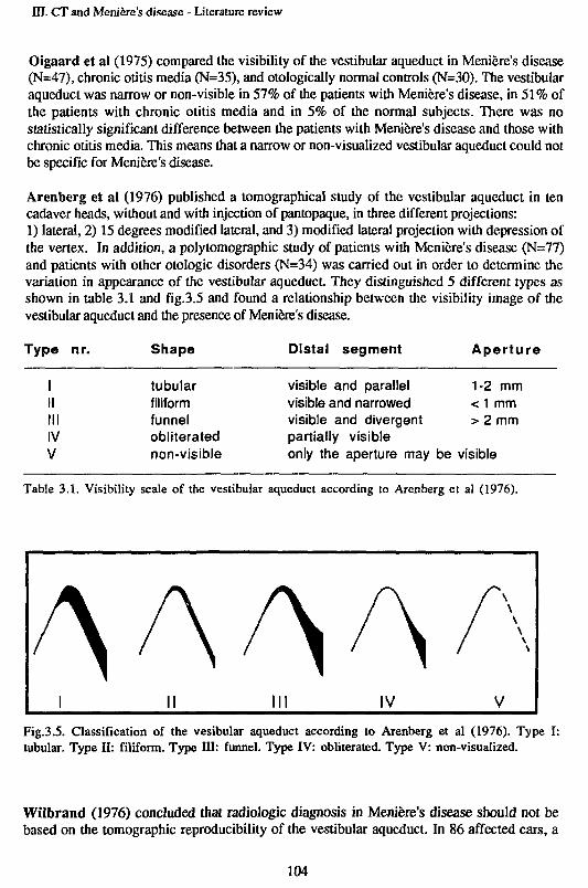
HI. CT and Meniere's disease - Literature review
Oigaard et al (1975) compared the visibility of the vestibular aqueduct in Meniere's disease(N=47), chronic otitis media (N=35), and otologically normal controls (N=30). The vestibularaqueduct was narrow or non-visible in 57% of the patients with Meniere's disease, in 51% ofthe patients with chronic otitis media and in 5% of the normal subjects. There was nostatistically significant difference between the patients with Meniere's disease and those withchronic otitis media. This means that a narrow or non-visualized vestibular aqueduct could notbe specific for Meniere's disease.
Arenberg et al (1976) published a tomographical study of the vestibular aqueduct in tencadaver heads, without and with injection of pantopaque, in three different projections:1) lateral, 2) 15 degrees modified lateral, and 3) modified lateral projection with depression ofthe vertex. In addition, a polytomographic study of patients with Meniere's disease (N=77)and patients with other otologic disorders (N=34) was carried out in order to determine thevariation in appearance of the vestibular aqueduct They distinguished 5 different types asshown in table 3.1 and fig.3.5 and found a relationship between the visibility image of thevestibular aqueduct and the presence of Meniere's disease.
Type nr. Shape Distal segment Aperture
IIIIIIIVV
tubularfiliformfunnelobliteratednon-visible
visible and parallel 1-2 mmvisible and narrowed < 1 mmvisible and divergent > 2 mmpartially visibleonly the aperture may be visible
Table 3.1. Visibility scale of the vestibular aqueduct according to Arenberg et al (1976).
AAAAFig.3.5. Classification of the vesibular aqueduct according to Arenberg et al (1976). Type I:tubular. Type II: filiform. Type HI: funnel. Type IV: obliterated. Type V: non-visualized.
Wilbrand (1976) concluded that radiologic diagnosis in Meniere's disease should not bebased on the tomographic reproducibility of the vestibular aqueduct. In 86 affected ears, a
104

HI. CT and Menicre's disease - Literature review
reduction in or lack of periaqueductal pneumatization was found in all cases. In only 66% ofthe control ears (N=32) a similar reduction of pneumatization was found. In 1978 Wilbrand etal observed that patients with Meniere's disease often had a shorter vestibular aqueduct ontomograms than healthy subjects. Patients with longstanding Meniere's disease had a shortervestibular aqueduct and a lower visibility of the aqueduct as compared with patients having ashort history of the disease.
Arenberg et al (1977) studied 100 temporal bones by microdissection, tomography andplastic molds. Normal subjects and patients with Meniere's disease were examinedtomographically as well. They concluded that in Meniere's disease there is, with theincreasing duration of the disease, a decrease in periaqueductal and opercular air cellpneumatization, with a concomitant shorter and straighter vestibular aqueduct. In normalindividuals the aqueduct could always be reproduced in its entire length by tomography. In themost sclerotic pyramids of patients with Meniere's disease, on the other hand, the aqueductcould not be visualized.
Valvassori & Clemis (1978) reviewed 3000 consecutive cases referred for tomographicstudies of the vestibular aqueduct because of cochleovestibular disorders and described a'narrow' and a 'wide vestibular aqueduct syndrome'. A very high incidence of correlation wasobserved between nonvisualized or filiform vestibular aqueduct and clinical disturbances of theinner ear like the type of Meniere's disease. Several patients with unilateral inner earsymptoms at the time of the study but with a bilateral nonvisualization of the aqueductsdeveloped similar symptoms in the opposite ear later.
Kraus & Dubois (1979) evaluated 190 randomly selected polytomograms and found anabnormal vestibular aqueduct in 43% of affected ears, 45% of contralateral (non-affected) ears,41% of ears with diseases other than Meniere's disease and 52% of normal ears. Theyconcluded that narrowing or nonvisualization of the vestibular aqueduct is a nonspecificrontgenographic sign that is seen in the same percentage in diseased and in normal ears, andthat it should not be used in diagnosing Meniere's disease.
Wilbrand (1980) tomographed fresh frozen temporal bone specimens and afterwardssectioned them with the cryomicrotome in the corresponding planes. This method alloweddirect translation of the information from the tomogram to the corresponding section level.Temporal bones of Meniere patients showed short vestibular aqueducts and, for the most part,no periaqueductal pneumatization. The operculum often consisted of a solid bony lamella.Temporal bones with poor perilabyrinthine and periaqueductal pneumatization and aconsequently small vestibular aqueduct also occurred to some extent among healthyindividuals.
Oku et al (1980) measured the size of the mastoid air system with a planimeter, excludingthe space of the middle ear, in tomograms of 27 patients with Meniere's disease, 27 patientswith other causes of sensorineural hearing loss and 25 otologicaily healthy persons. Nostatistical differences were seen between these three groups.
105

HI. CT and Meniere's disease - Literature review
Sackett et al (1980) radiographically studied 72 patients with unilateral or bilateralMeniere's disease before saccus surgery. They found that the size, shape and patency of thevestibular aqueduct were of no value in predicting the presence of bilateral disease.
Austin (1980, 1981) evaluated polytomographic examinations of the vestibular aqueduct in105 patients with Meniere's disease and found a normal aqueduct in 12% as compared to 95%in control subjects. He concluded that tomography of the vestibular aqueduct should beregarded a valuable diagnostic tool in Meniere's disease and that success or failure of theendolymphatic shunt operation is correlated with patency of the vestibular aqueduct.
Dauphin et al (1981) studied 27 patients with Meniere's disease and 15 without anycochleovestibular disturbance. They found an aqueductal stenosis in 53% and a petrous densityin 71% of the Meniere cases. There was a close correlation between petrous density andstenosis of the vestibular aqueduct. Another important positive correlation was found betweendensity andperilabyrinthine developmental abnormality and Meniere's disease. Two years laterthese authors (Dauphin et al, 1983) framed up a radio-tomographic triptych of the factors:peripetrosal condensation, stenosis of the vestibular aqueduct and diminution of the posteriorand postero-superior petrosal thickness. This tends to confirm the hypothesis of aninflammatory process in infancy before the complete development of the temporal bone as apositive cause. A parallel study of the results of the glycerol tests showed a complete absenceof any correlation between this radiographic triptych and the positivity of the test.
Hall et al (1983) performed a radiographic study of the endolymphatic duct in Meniere'sdisease. The vestibular aqueduct was visible in 88% of the cases, and they considered a funnelor tubular shape as normal. On the other hand, filiform shapes were found in 47% of patientswith Meniere's disease compared with 31% in the control group. They stated that this formmay be considered as an intermediate stage towards obliteration of the aqueduct. Ahypopneumatization was found on the affected side as well as on the normal side. This led tothe supposition that the same syndrome could be found on both sides. The overall conclusionwas that lateral tomography is not a sufficiently positive aid in diagnosing Meniere's disease.
Sando & Ikeda (1984) studied histologically 27 temporal bones of patients with Meniere'sdisease and 88 normal temporal bones. Measurements were made of the length, width, angleand position of the external aperture of the vestibular aqueduct. The conclusion was that asmall vestibular aqueduct was more often observed in temporal bones of patients withMeniere's disease than in the normal ear.
Arenberg et al (1984) concluded that the results of multidirectional tomography areconfusing and controversial because of the use of different tomographical techniques. Hecompared multidirectional tomography and high resolution CT in 60 patients and concludedthat the clinical limitations of multidirectional tomography for inner ear diagnosis andprognosis for endolymphatic sac surgery are evident, and that high-resolution CT scanningopens the possibility of better visualization of inner and middle ear structures.
Valvassori & Dobben (1984) compared the tomographical findings of a previous study(Valvassori & Clemis, 1978 a,b) with CT examination of 47 patients with Meniere's disease.
106

HI. CT and Meniere's disease - Literature review
Only direct horizontal (=transverse) and coronal sections could be directly obtained.Visualization in other otoradiological planes was carried out by means of imagereconstruction (reformatting). They found no significant difference between multidirectionaltomography and CT findings on the visualization of the vestibular aqueduct.
Nidecker et al (1985) demonstrated by means of high-resolution CT investigationmorphological alterations of the temporal bone in 10 patients with Meniere's disease ascompared to 14 non-Meniere patients. They found a distinctly decreased visibility of thevestibular aqueduct and a dense retrolabyrinthine sclerosis in the Meniere group. Findingswere bilateral in all patients. Gradation of the aqueductal visibility was as follows: 0=notvisible; l=portions poorly visible; 2=entirely visible aqueduct.
CONCLUSIONS
From the above review of the literature it may be clear that the clinical usefulness and validityof radiotomography of the vestibular aqueduct is not proven. The results are often confusingand controversial. A large variation in visibility of the vestibular aqueduct in patients withMenierc's disease was found.
'Obliteration' or 'non-visibility' of the vestibular aqueduct was seen in 31% to 65% of theMeniere-cases, while a 'normal' or well-visible aqueduct was present, in 70% to 100% ofpatients with cochleovestibular problems other than Meniere's disease and in normal ears.
The statistical correlation of rontgenographic findings and the correlation between success orfailure of endolymphatic shunt operations and the patency of the aqueduct initially seemed toopen a new dimension in the treatment of Meniere's disease. As the therapy of the saccusoperation is now considered highly questionable, radiological examination of the vestibularaqueduct is at this moment only of additional diagnostic value.
From the numerous studies carried out until now, however, the following conclusions seemto be justified:
1. The vestibular aqueduct can, to a certain degree, be visualized by multidirectionaltomography or polylomography. Great variations as to visibility and size have been reported,however. This may be due to the different tomographical techniques of investigation and thevarious classifications of the visibility of the vestibular aqueduct, making a comparisondifficult or impossible. Another cause may be the difference in patients' selection betweenthese studies. Tomography is apparently not a specific diagnostic technique for diagnosingMeniere's disease, although, unfortunately, clinical conclusions have been drawn on the basisof such radiologic observations which are at the limits of the spatial and contrast resolution ofthese methods.
107

HI. CT and Meniere's disease - Literature review
2. The vestibular aqueduct seems to be more difficult to visualize in Meniere's disease than innormal ears, although not all authors agree with this conclusion.
3. The aqueductal length seems to be shorter in patients wilh Meniere's disease as compared tonormal ears. It is postulated that the vestibular aqueduct tends to diminish in length in thecourse of the disease.
4. In most studies the findings in non-affected ears of patients wilh Meniere's disease weresimilar to those in the affected ears.
108

HI. CT and Meniere's disease - Objectives
OBJECTIVES OF THIS STUDY
As has became evident from the foregoing, radiologic visualization of the vestibular aqueducthas been the subject of much controversy in the last 15 years. The new possibilities of highresolution CT combines a high contrast-resolution with a better spatial resolution and thepossibility of direct imaging in the desired plane without disturbances by overlayingstructures. For this reason we have investigated the visualization problems of the vestibularaqueduct by computed tomography techniques and compared our findings in normal ears andears of patients with Meniere's disease with those from previous studies.
The following questions have been studied:
1. a. Is it possible to visualize the vestibular aqueduct by means of high-resolution CTscanning in a reproducible way?b. In which otoradiological plane(s) can this structure best be imaged?c. Is it possible to measure the dimensions of the vestibular aqueduct by means of CT?
2. To what extent does the visibility (width) and length of the vestibular aqueduct vary innormal ears?
3. Is the visibility and length of the vestibular aqueduct in affected ears of patients withMeniere's disease different from that in normal ears?
4. Is the visibility and length of the vestibular aqueduct in the non-affected ears of patientswith Meniere's disease different from that in normal ears?
3. Does the visibility and length of the vestibular aqueduct in patients with Meniere's diseasediffer with-age,-duration of the disease and-amount of hearing loss?
109

III. CT and Meniere's disease - Materials
MATERIALS
From 1982 to 1985 a consecutive series of patients with Meniere's disease was investigated inthe Departments of ORL and Radiology of the Utrecht University Hospital.
1. SELECTION CRITERIA
Inclusion criteria
In order to be included the patients had to meet the following criteria according to our Utrechtdefinition (van Deelen, 1986):
1. Unilateral or bilateral sensorineural hearing loss with tinnitus and (a history of)vertiginous attacks of unknown origin.
2. Positive recruitment and normal perstimulatory adaptation as measured by ABLB test,Bekesy audiometry, stapedius reflex measurement and tone decay test.
3. Normal X-ray anatomy of ihe temporal bone in the Schiiller and Stenvers projection.4. No other otological, neurological or internal disorder that could account for one of the
symptoms.
Exclusion criteria
Excluded from the study were the ears of patients with:1. History or signs of chronic otitis media or mastoiditis.2. Bone diseases involving the petrous bone (Otosclerosis, Paget's disease, Osteogenesis
Imperfecta etc.).3. Previous ear surgery.
Affected ears of patients with unilateral Meniere's disease of which the non-affected ear wasexcluded, were included in this study too.
110

HI. CT and Meniere's disease - Materials
2. PATIENTS and EARS
On the base of the above mentioned criteria, 55 patients entered this study. Of these patients 9had a bilateral, 46 an unilateral Meniere's disease. The total number of affected ears thusamounted to 64, that of the non-affected ears to 46. On the basis of the exclusion criteria thedata of 6 non-affected ears had to be discarded. The ultimate number of non-affected earsaccepted thus amounted to 40 (table 3.2).
Meniere's disease Patients Affected ears Non-affected ears
Unilateral 46 46 46
Bilateral 9 18 0
Total 55 64 46
Included 55 64 40Table 3.2. Numbers of patients, affected and non-affected ears accepted for this study.
Age distribution
The age distribution of the patients is presented in table 3.3. The distribution of the patientsin the age categories between 30 and 69 years is proportional.
Age 20-29 30-39 40-49 50-59 60-69 70-79
Patients 4 14 11 13 11 2
Table 3.3. Age distribution of the patients (N=55).
Sex distribution
Of the 55 patients included, 30 were male (25 with unilateral and 5 with bilateral Meniere'sdisease) and 25 female (21 with unilateral and 4 with bilateral Meniere's disease) - (table 3.4).
Meniere's disease Male Female Total
Unilateral 25 21 46Bilateral 5 4 9
Total 30 25 55
Table 3.4. Sex distribution of the patients and laterally of the disease.
I l l

III. CT and Meniere's disease - Materials
Duration of disease
The time in years elapsed since the onset of Meniere's disease in the ears of this study ispresented in table 3.5. In 31 ears the disease existed for less than five years, in 33 for morethan five years.
Duration (years) 0-2 3-5 6-8 9-14 >14
Ears (N) 17 14 7 12 14
Table 3.5. Duration of Meniere's disease in the 64 affected ears.
3. NORMAL EARS USED AS CONTROLS
As controls CT scans of 50 ears from 30 cases with normal inner ear and vestibular functionwere used. From these ears 10 were the healthy, contralateral ears of patients with unilateralchronic otitis media, Bell's palsy, middle ear trauma, sudden deafness and congenital deafness.The other 40 ears belonged to 20 cases in whom CT scanning was carried out and nootological nor vestibular disorder was found, (table 3.6).
Normal (control) ears Cases Ears
Contralateral ears 10 10Both ears 20 40
Total 30 50
Table 3.6. Numbers of cases and ears used as controls.
Age distribution
The age distribution of the 30 controls is given in table 5. Of these 67% were between 30 and70 years of age as compared to 89% in the group of patients with Meniere's disease (table3.7).
Age 0-9 10-19 20-29 30-39 40-49 50-59 60-69 70-79
Cases 1 1 6 10 2 5 3 2
Table 3.7. Age distribution of the 30 cases used as controls.
112

HI. CT and Meniere's disease - Materials
4. SUMMARY
PATIENTS WITHMENIERBS DISEASE
55
BILATERALLYAFFECTED
9
UNILATERALLYAFFECTED
46
AFFECTEDEARS64
INCLUDED
NORMAL (CONTROLS)
30
BILATERAL
20
NON-AFFECTEDEARS46
EXCLUDED
64 40
UNILATERAL
10
CONTROLSNORMAL EARS
50
50
Fig.3.6. Composition of the materials (patients and ears) as used in this study.
113

HI. CT and Meniere's disease - Methods
METHODS
1. PLANES OF CT EXAMINATION
Previous polytomographic studies were usually carried out in a lateral or modified lateralprojection. We have experimented with these planes as well as with other otoradiologic planeson cadaver heads as described in part I and found no evident difference in visualization of thevestibular aqueduct. As in all our other examinations the transverse plane (Him) was used asthe first plane of investigation. The axio-petrosal plane (Poschl) was chosen as the secondprojection for studying the vestibular aqueduct because of the more comfortable position ofthe patients and the easier reproducibility of this plane.
2. VISIBILITY SCALE OF THE VESTIBULAR AQUEDUCT
The basic problem of developing a method of visual examination of the vestibular aqueduct isthe lack of a CT image of the 'normal' aqueduct. Histologic studies have demonstrated that thenormal vestibular aqueduct diameter ranges from 0.65 to 4.55 mm (Anson, 1965; Sando &Ikeda, 1984). The spatial resolution of high-resolution CT scanners is limited to 0.6 mm. Anormal vestibular aqueduct should therefore be visible on CT if contrast is not decreased byfactors within the aqueduct (e.g. fibrosis).In order to become informed about the image of a normal aqueduct, the normal (control) earswere examined first. If the aqueduct was visualized with good contrast, it was considered'normal'. Comparisons were made with previous polytomographic studies (Vignaud, 1971)and a subjective scale of visibility was then devised. Five classes of aqueductal visibility weredistinguished:
Class 1: 'non-visible'- The vestibular aqueduct is not visible, either in the transverseor in the axio-petrosal plane (fig.3.7 ab).Class 2: 'aperture visible only' - Only the aperture at the postero-medial wall of thepetrous bone is visible in at least one of the two planes. The remaining distal part of the ductis not visible (fig.3.8 ab).Class 3: 'narrow' - The distal part of the vestibular aqueduct is visible in at least one ofthe two planes, but the contrast with the surrounding bone is poor because of a 'narrowing' ofthe aqueductal lumen or an increase in radiodensity of the aqueductal contents (fig.3.9 ab).Class 4: 'normal' - The distal part is 'normally' visible in at least one of the twoplanes of investigation (fig.3.10 ab).Class 5: 'wide' - The distal part is wide as compared to those with a normal visibility(fig.3.11 ab).
114

III. CT and Menicre's disease - Methods
Exemples of these 5 classes, as seen on CT images, are given in the transverse (Hirtz) planeand axio-petrosal (Poschl) plane in figs. 3.7 - 3.11. Arrows indicate the location of thevcstibular aqueduct.
TRANSVERSE PLANE (Hirtz) AXIO-PETROSAL PLANE (Poschl)
Fig.3.7 (ab). Class 1: non-visible
Fig.3.8 (ab). Class 2: Aperture visible only
Fig.3.9 (ab). Class 3: 'narrow'
115

III. CT and Menicre's disease - Methods
TRANSVERSE PLANE (Hirtz) AXIO-PETROSAL PLANE (Foschl)
Fig.3.10 (ab). Class 4: 'normal'
Fig.3.11(ab). Class 5: wide'
3. VISUAL EVALUATION OF THE CT SCANS
The classification of the vestibular aqueduct into one of the five classes was performed blindlyand independantly by two investigators (F.W. Zonneveld and the author). CT images ofaffected, non-affected and control ears were mixed at random, with the patients' personal dataconcealed. Both investigators were asked to classify all aqueducts according to the visibilityscale. This procedure was performed twice.
116

HI. CT and Meniere's disease - Methods
4. MEASURING THE LENGTH OF THE VESTIBULAR AQUEDUCT
The proximal part of the vestibular aqueduct has a diameter of 0.35 mm (range: 0.25-0.50mm) - (Anson, 1965). These dimensions are beyond the spatial resolution (0.6 mm) of theCT scanner and can therefore not be visualized. For this reason only the length of the distalpart was measured, if possible, in the transverse plane. This measurement was conducted asfollows:
Scans were made with a slice thickness of 1.5 mm. In fig. 3.12 an imaginary vestibularaqueduct is drawn. Point PI is located at the isthmus and point P2 at the caudal border of theaperture. Although the distal part of the vestibular aqueduct is not always straight, thedistance between the two points PI and P2 was assumed as the approximation of the lengthof the aqueduct.
To determine this distance, the level of the isthmus is determined first. The coordinates of thispoint (PI) are then established by pointing with the lightpen on the monitor screen at thispoint. A software facility then calculates the three coordinates in millimeters. Thesecoordinates are called: X j , Yj and Zj.
Fig.3.12. Schematic drawing for measuring the length of the vestibular aqueduct. PI is theisthmus, P2 the caudal margin of the aperture. The aqueduct is projected on a plane parallel tothe scanning plane. The distance between PI and P2 is considered the approximation of thelength of the vestibular aqueduct.
117

HI. CT and Meniere's disease - Methods
We then search for the level of the aperture (P2) in the adjacent CT sections. The dimensionof the aperture has a large variation. When the aperture is visible on more than onesubsequent scanning sections, the most medio-caudal part of the aperture is considered to bethe distal ending of the aqueduct. The coordinates X2, Y2 and Z2 of point P2 are thendetermined in the same way as for point PI.
Now AX, AY and AZ can be calculated (fig.3.12):
AX ( difference between Xj and X2 ) = length of line BD
AY (difference between Yj and Y 2 ) = length of line CD
AZ (difference between Z j and Z2) = length of line P | A
The length of line P ^ can be calculated using the formula:
( p l p 2) 2 =
We measured this distance in the two perpendicular planes (transverse plane and axio-petrosalplane) separately. The mean value of both calculations was considered to be the length ofdistal part of the vestibular aqueduct.
It will be clear that the length cannot be measured in ears with a non-visible aqueduct (class1). In ears of class 2 (only visible aperture) the isthmus is invisible. Because of the fact thatthe isthmus normally is located just medially of the common crus, the coordinates of thispoint were taken as the coordinates of the isthmus.
5. AUDIOMETRY
From all audiometric data (pure tone and speech audiometry, ABLB test, Bekesy audiometry,stapedius reflex measurement, tone decay test) we used the bone conduction thresholdmeasurements to correlate with the CT data. If hearing loss was fluctuating, we chosed thedata of the 'best' audiogram in a series of measurements from a period of at least half a yearfor further analysis.
118

HI. CT and Meniere's disease - Methods
Transverse plane (Hirtz)
Fig.3.13. Level of the isthmus.
Fig.3.14. Oblique section through the vestibular aqueduct.
Fig.3.15. Level of the caudal margin of the aperture.
Figs. 3.13 - 3.15. Exemple of the course of the distal part of the vestibular aqueduct visualizedin three subsequent transverse scans with a slice-thickness of 1.5 mm. Fig. 3.13 shows thedistal part near the isthmus. Fig.3.14 an oblique cross-section through the vestibular aqueduct,Fig.3.15 the caudal margin of the aperture. SSC/PSC/LSC = Superios/Posterior/Lateralsemicircular canal. VA = Vestibular aqueduct. C = Cochlea. CC = Common crus. IAC = Internalauditory canal.
119

HI. CT and Meniere's disease - Results
RESULTS
1. VISIBILITY OF THE VESTIBULAR AQUEDUCT
1.1. Control ears
In the 50 control ears the visibility of the vestibular aqueduct was classified as 'normal' in74%, 'non-visible' in 2%, 'aperture visible only' in 6%, 'narrow' in 16% and 'wide' in 2%(fig.3.16).
10090"80706050403020
10 Ho
NORMAL
74.0
APERTUREVISIBLE
NON-VISIBLE O N L Y
2.0
NARROW
16.0
6.0WIDE
2.0
CLASS
Fig.3.16. Visibility of the vestibular aqueduct in 50 control ears (percentages).
1.2. Affected ears of patients with Meniere's disease
The visibility of the vestibular aqueduct in the 54 Meniere ears appeared to be completelydifferent: it was classified as 'normal' in only 25%, 'non-visible' in 15.6%, 'aperture visibleonly' in 20.3%, 'narrow' in 37.5% and 'wide' in 1.6%. As compared to the control ears thevestibular aqueduct in affected ears of patients with Meniere's disease was thus found to beconsiderably less visible or more narrow (fig.3.17).
120

HI. CT and Meniere's disease - Results
100
9 0 -
80
70
60
50
40 H
3 0 "
2 0 -
1 0 -
0
NON-VISIBLE
15.6
APERTUREVISIBLE
ONLY
20.3
NARROW
37.5 NORMAL
25.0
WIDE
1.6
1 5 CLASS
Fig.3.17. Visibility of the vestibular aqueduct in 64 affected ears of Meniere's patients(percentages).
1.3. Non-affected ears of patients with unilateral Meniere's disease
In the 40 non-affected ears of the patients with unilateral Meniere's disease a similardistribution to that of the affected ears was found (fig.3.18): in 35% the veslibular aqueductwas classified as 'normal', in 17.5% as 'not visible1, in 12.5% as 'aperture visible only', in30% as 'narrow' and 'wide' in 5%. As compared to the affected ears, the percentage ofnormally visible aqueducts is 10% higher, but still 39% lower than in control ears.
100
90
80
70 •
60 ••
% 50 •
40 •
30
20
10
0
NON-VISIBLE
17.5
APERTUREVISIBLE
ONLY
12.5
NARROW
30.0
WIDE
5.0
1 5 CLASS
Fig.3.18. Visibility of the vestibular aqueduct in 40 non-affected ears of Meniere's patients(percentages).
121

III. CT and Meniere's disease - Results
The numbers of affected, non-affected and control ears in each visibility class (1-5) arepresented in table 3.8 in combination with the percentages as shown in figs. 3.16 - 3.18.
Ears Controls Affected Non-affected
ClassClassClassClassClass
12345
(non-visible)(aperture only)(narrow)(normal)(wide)
N
138
371
%
2.06.0
16.074.0
2.0
N
10132416
1
%
15.620.337.525.0
1.6
N
75
12142
%
17.512.530.035.0
5.0
Total 50 100% 64 100% 40 100%
Table 3.8. Visibility of the vestibular aqueduct in the control ears, affected ears and non-affectedears of patients with Meniere's disease.
2. LENGTH OF THE VESTIBULAR AQUEDUCT
As the length of the vestibular aqueduct could not be measured in the ears with a non-visibleduct (Class 1), 49 control ears, 54 affected ears and 33 non-affected ears were studied. Theresults are given in table 3.9.
Ears N Mean length (mm) SD
Control ears 49 7.7 1.6Affected ears 54 5.5 2.1Non-affected ears 33 5.7 2.4
Table 3.9. Mean length (in mm) and standard deviations of control ears, affected ears andnon-affected ears of patients with Meniere's disease.
The mean length of the vestibular aqueduct in affected ears was found to be 5.5 mm (SD: 2.1)as compared to 7.7 mm (SD: 1.6) in control ears. This difference is highly significant(p<0.001). In the non-affected ears the mean length was 5.7 mm (SD: 2.4), again a highlysignificant difference with that in normal ears (p<0.001). NO significant difference was foundbetween affected and non-affected ears (p>0.05).
122

HI. CT and Menicre's disease - Results
Correlation with age.
The length of the vestibular aqueduct was not correlated with age (p>0.05) either in thecontrol ears, or in the ears of patients with Meniere's disease. Coefficients (R) and thesignificance (p) of these correlations are given in table 3.10.
Ears
Control earsAffected earsNon-affected ears
0.200.260.25
> 0.05> 0.05> 0.05
Table 3.10. Correlation coefficient (R) and significance (p) of the correlation between length ofthe vestibular aqueduct and the age in control ears, affected ears and non-affected ears.
Correlation with BC hearing loss.
The length of the vestibular aqueduct in control ear, affected and non-affected ears showed nosignificant correlation (p>0.05) with the 3-frequency bone conduction hearing loss (500,1000and 2000 Hz) as shown in table 3.11.
Ears
Control earsAffected earsNon-affected ears
0.230.210.14
> 0.05> 0.05> 0.05
Table 3.11. Coefficient (R) and significance (p) of the correlation between the length of thevestibular aqueduct and the mean 3-frequency BC hearing loss in control ears, affected ears andnon-affected ears.
Correlation with duration of Meniere's disease.
Ears R p
Affected ears 0.36 < 0.01
Table 3.12. Coefficient (R) and significance (p) of the con-elation between the length of thevestibular aqueduct and the duration of Meniere's disease in affected ears.
123

III. CT and Mcnicre's disease - Results
As to the correlation between the length of the vestibular aqueduct and the duration ofMeniere's disease, a low but significant negative correlation (R=0.36, p<0.01) was present(table 3.12). In affected ears of Meniere's patients the length of the vestibular aqueduct tendsto decrease with the duration of the disease. The mean length in affected ears with a durationof disease shorter than 5 years was 6.2 mm (SD: 2.1), in ears with a duration of diseaselonger than 5 years 4.8 mm (SD: 1.9). This difference is statistically significant (p<0.05) -(table 3.13).
Duration N Length (mm) SD
< 5 years 27 6.2 2.1> 5 years 27 4.8 1.9
Table 3.13. Length of the vestibular aqueduct in ears with a duration of Meniere's diseaseshorter and longer than 5 years.
Relation between visibility and length of the vestibular aqueduct.
No significant correlation was found (p>0.05) between visibility and aqueductal length (table3.14). A 'normal' visible aqueduct was found to be of the same length as a narrow aqueduct oras an aqueduct of which only the aperture was visible.
Ears R
Control earsAffected earsNon-affected ears
0.020.200.12
> 0.05> 0.05> 0.05
Table 3.14. Coefficient (R) and significance (p) of the correlation between the length of thevestibular aqueduct and the visibility class in control ears, affected ears and non-affected ears ofpatients with Meniere's disease.
124

HI. CT and Meniere's disease - Conclusions
CONCLUSIONS
1. The vestibular aqueduct can be visualized in the majority of the otoradiological planes.Due to its variety in course, at least two planes perpendicular to each other are needed toobtain appropriate information about its course, size and shape. We have chosen to usethe combination of the transverse (Hirtz) plane and the axio-petrosal (Poschl) planebecause of the better reproducibility of these planes as compared to other planes.
2. In normal petrous bones the vestibular aqueduct was normally visible in 74% of theexamined ears. A narrow or non-visible aqueduct was found in 24%, a wide one in 2%.
3. In affected ears of patients with Meniere's disease, the aqueduct was normally visible inonly 25%. A narrow or non-visualized aqueduct was found in 73.4%. Compared to thefindings in the normal ears, the vestibular aqueducts are thus much more difficult tovisualize.
4. In the non-affected ears of patients with unilateral Meniere's disease the results wereremarkably similar to those obtained in the affected ears: a normally visible aqueduct wasfound in 35%, a narrow or non-visible duct in 60%, whereas a wide aqueduct was seen in5% of the ears.
5. The mean length of the distal part of the vestibular aqueduct in normal ears was found 7.7mm with a standard deviation of 1.6. The part proximal to the isthmus could not bevisualized with our technique as its dimension is beyond the spatial resolution of the highresolution CT scanner.
6. In affected ears of patients with Meniere's disease the distal part of the vestibular aqueductis significantly shorter than in normal ears (mean: 5.5 mm; SD: 2.1).
7. In the non-affected ears this length was found the same as in affected ears.
8. No significant correlation was found between aqueductal length and age either in normalears or in affected or non-affected ears of patients with Meniere's disease.
9. In longstanding Meniere's disease the vestibular aqueduct was shorter (p<0.05) than inMeniere's disease of shorter duration. The mean length of the vestibular aqueduct inaffected ears with a duration of the disease shorter than 5 years was 6.2 mm (SD: 2.1)whereas it was 4.8 mm (SD: 1.9) in ears with a duration longer than 5 years.
10. The length of the vestibular aqueduct is not correlated with the mean 3-frequency boneconduction hearing loss (500,1000 and 2000 Hz).
125

HI. CT and Meniere's disease - Discussion
DISCUSSION
1. VISUALIZATION AND LENGTH OF THE VESTIBULAR AQUEDUCT
Scanning planes for visualization of the vestibular aqueductAs the course of the vestibular aqueduct varies widely, it is practically impossible to find astandardized scanning plane that images the entire aqueduct in one single slice. We thereforeused a combination of two planes. As the vestibular aqueduct can be visualized in all planesdescribed in part I and since they are all perpendicular to the transverse plane, eachcombination with the transverse plane should theoretically be adequate. We have chosen theaxio-petrosal (POschl) plane as the second plane of investigation because of its goodreproducibility and the relatively comfortable positioning for the patient.
A CT image is computed from data in one slice of tissue with a thickness of 1.5 mm. Mostlythe vestibular aqueduct will not be lying entirely within one slice as it crosses the scanningplane. It is therefore necessary to scan a circumscribed part of the petrous bone in contiguousslices in both directions in order to image all parts of the vestibular aqueduct.
Visualization of the vestibuiar aqueductA canalicular structure within a bony mass will be visible on CT images if- its diameter is not smaller than the spatial resolution of the scanner and- its contents possess enough contrast with the surrounding bone.
Normally the membranous endolymphatic duct has a density similar to that of water.Therefore it will have a good contrast with the very dense surrounding petrous bone. Adecrease in contrast caused by an increase of the density of its contents will result in adiminished visibility on CT scans. An increase of soft tissue volume, e.g., fibrosis withinthe endolymphatic duct could have this effect
Similarity, a decrease of the aqueductal diameter, e.g., due to bone apposition, will result in apoorer visualization. Taking into account that we work at the borders of the spatial resolutionof the CT scanner, it will not be possible to distinguish between these two possible causes ofimpaired visibility. If the caliber of the aqueduct reaches the dimensions of the spatialresolution of the CT scanner, there will be a decrease in contrast that is to some extent causedby the partial volume averaging effect.
In our study the 'filiform' or 'thread-like' aqueduct was frequently seen. The name 'filiform'does not appear correct, however. The cause of a poor visibility of the vestibular aqueductseemed to be more a matter of contrast-reduction between the aqueductal lumen and thesurrounding bone than a real narrowing. In some cases, on the contrary, we had theimpression of even a widening of the lumen combined with a decrease in contrast by apossible fibrous obliteration. When we found a 'filiform' aqueduct it was classified as 'narrow'.
Another problem in classifying the aqueduct is discerning between a very short aqueduct and a
126

HI. CT and Meniere's disease - Discussion
partial obstruction. A 'funnel-shaped' aqueduct, as it was called in the investigation ofArenberg et al (1976), was not found in this study. The reason for this difference in resultscould be the following: the distal part of the vestibular aqueduct has a flattened and twisted(propellor-like) shape (Clemis & Valvassori, 1968; Ogura & Clemis,1971). Since in CT theaqueduct is studied in two perpendicular planes, conic images are obtained of its lumen whereit crosses the scanning slice. With the classical tomography techniques this may be possibleindeed because of the use of much thicker slices. The entire vestibular aqueduct can be depictedin one single slice. This could be considered as a disadvantage of CT technique. If, however,the entire aqueduct is visualized in one thick slice, only information of its two-dimensionalprojection is obtained. Adequate measurements of its length can therefore not be carried out inthis way.
Measuring the size of the vestibular aqueductWe developed a method to calculate the length of the vesubular aqueduct if it crosses severalCT slices. This method appeared to be well reproducible. In this way we were able tocalculate the adequate approximation of the real length of the distal part of the duct. Thismethod differs from the measurements as used in previous polytomographic techniques.Instead of measuring the length directly on the image we established the three-dimensionalcoordinates of a voxel at the isthmus and at the aperture of the vestibular aqueduct. Knowingpixel size and slice thickness, the distance between these two voxels can be easily calculated.
We did not measure the diameter of the vestibular aqueduct as Nidecker et al (1985) did. Wefelt that our techniques were not adequate enough to measure the width of a 'narrow' aqueductor of aqueducts with only a visible aperture.
2. RESULTS IN NORMAL EARS
Visibility of the vestibular aqueductIn our study the vestibular aqueduct was found 'normally' visible in about 75 percent of thenormal control ears. Taking into account that these ears were not specially scanned to studythe vestibular aqueduct, this percentage might have been even higher if special attention hadbeen paid to the visualization of the aqueduct.In the majority of previous tomographical investigations this percentage was between 90 and100 (table 3.15). Only in the studies of Kraus & Dubois (1979) and Hall et al (1983) lowerpercentages were found.

III. CT and Meniere's disease - Discussion
Author Year Control groupvisualized
Brunner & PedersenStahle & WilbrandRumbaugh et alOigaard et alArenberg et alValvassori & ClemisKraus & DuboisDauphin et alHall et al
197419741974197519771978197919811983
9 1 %100%
97%97%
100%92%70%90%54%
This study 74%
Table 3.15. Visualization of the vestibular aqueduct in normal control ears as found in previoustomographical studies and in our CT study.
Length of Hie vestibular aqueductIn our study the length of the distal part of the vestibular aqueduct in normal ears was foundto be 7.7 mm (SD: 1.6).The mean length of the vestibular aqueduct has been reported higher in five studies andsmaller in two studies (table 3.16). Our result agrees with the most recent histological studyby Sando & Dceda (1984).
Author
Ogura & ClemisWilbrand et alStahle & WilbrandArenberg et alPlantenga & BrowningRizvi & SmithSando & Ikeda
This study
year
1971197419741977197919811984
Method
dissectiondissectiontomographydissect, and tomogr.histologichistologichistologic
CT
Length (mm)
8.78.478.78.16.96.957.8
7.7
Table 3.16. Mean length of the vestibular aqueduct in normal ears found in previoushistological, dissectional and tomographical studies and in our CT study.
128
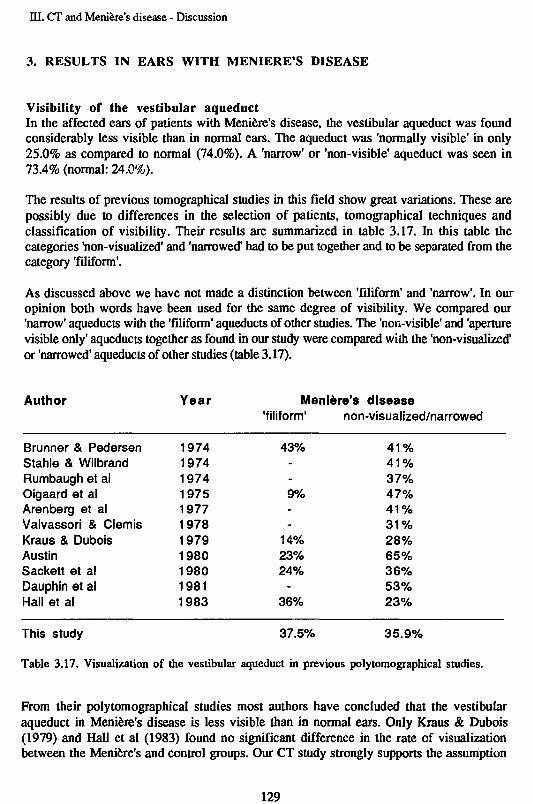
HI. CT and Meniere's disease - Discussion
3. RESULTS IN EARS WITH MENIERE'S DISEASE
Visibility of the vestibular aqueductIn the affected ears of patients with Meniere's disease, the vestibular aqueduct was foundconsiderably less visible than in normal ears. The aqueduct was 'normally visible' in only25.0% as compared to normal (74.0%). A 'narrow' or 'non-visible' aqueduct was seen in73.4% (normal: 24.0%).
The results of previous tomographical studies in this field show great variations. These arepossibly due to differences in the selection of patients, tomographical techniques andclassification of visibility. Their results are summarized in table 3.17. In this table thecategories 'non-visualized' and 'narrowed' had to be put together and to be separated from thecategory 'filiform1.
As discussed above we have not made a distinction between 'filiform' and 'narrow'. In ouropinion both words have been used for the same degree of visibility. We compared our'narrow' aqueducts with the 'filiform' aqueducts of other studies. The 'non-visible' and 'aperturevisible only' aqueducts together as found in our study were compared with the 'non-visualized'or 'narrowed' aqueducts of other studies (table 3.17).
Author Year Meniere's disease'filiform' non-visualized/narrowed
Brunner & PedersenStahle & WilbrandRumbaugh et alOigaard et alArenberg et alValvassori & ClemisKraus & DuboisAustinSackett et alDauphin et alHall et al
19741974197419751977197819791980198019811983
43%--9%--
14%23%24%
-36%
4 1 %4 1 %37%47%4 1 %3 1 %28%65%36%53%23%
This study 37.5% 35.9%
Table 3.17. Visualization of the vestibular aqueduct in previous polytomographical studies.
From their polytomographical studies most authors have concluded that the vestibularaqueduct in Meniere's disease is less visible than in normal ears. Only Kraus & Dubois(1979) and Hall et al (1983) found no significant difference in the rate of visualizationbetween the Meniere's and control groups. Our CT study strongly supports the assumption
129

HI. CT and Meniere's disease - Discussion
that the vestibular aqueduct in Meniere's disease is narrowed, in particular since the selectionof Meniere's patients and control ears was done on strict inclusion and exclusion criteria. Inaddition, the CT scanning was carried out in two perpendicular planes and the evaluation wasperformed blindly by two investigators by mixing at random the scans of affected ears ofMeniere's patients and those of the control ears.
As discussed before we were not able to distinguish between a bony and soft tissue narrowingor obliteration of the vestibular aqueduct because of the partial volume averaging effects.Histological studies by Rizvi & Smith (1981) and Sando & Ikeda (1984) have confirmed thatin temporal bones with endolymphatic hydrops the distal part of the vestibular aqueduct isnarrower than in normal bones. They found no changes in the proximal part of the aqueduct.
In the study of Valvassori and Dobben (1984) no significant difference in results between CTand polytomography (Valvassori & Clemis, 1978b) was found in visibility of the vestibularaqueduct. With both methods, the vestibular aqueducts in patients with Meniere's disease werefound to be narrower than in normal subjects. The same findings were found in the CT studyofNideckeretal(1985).
Length of the vestibular aqueductIn our study the mean length of the distal part of the vestibular aqueduct in affected ears ofpatients with Meniere's disease appeared to be 5.5 mm (SD: 2.1). Assuming on the basis ofanatomical studies of Anson (1965) that the length of the proximal part is 1.5 mm, the meantotal length of the aqueduct as measured in our study thus amounted to 7.0 mm. This result isin agreement with most of the histological studies summarized in table 3.18. Only Rizvi andSmith (1981) found a considerable shorter length of 5.65 mm. The other findings varybetween 6.5 and 7.3 mm, whereas Rask-Anderson et al (1977) measured 8.1 mm in apolytomographical study.
Author
Ogura & ClemisStable & WilbrandArenberg et alPlantenga & BrowningRask Andersen et alRizvi & SmithSando & Ikeda
year
1971197419771979197919811984
Method
dissectiontomographydissect, and tomogr.histologicaltomographyhistologicalhistological
Length (mm)
7.36.86.86.78.15.656.5
This study CT 5.5
Table 3.18. Mean length of the vestibular aqueduct in patients with Meniere's disease fromprevious histological, dissectional and tomographical studies and in our CT study.
130

HI. CT and Meniere's disease - Discussion
Correlation between visibility and age, duration, hearing lossNeither the visibility nor the length of the vestibular aqueduct was found to correlate with agein our study. The amount of bone conduction hearing loss was not correlated either withaqueductal length or visibility. This agrees with the tomographical results of Stahle &Wilbrand (1974).
The vestibular aqueduct was found to be longer in ears with Meniere's disease of less than fiveyears duration than in ears with a longer duration of the disease. This finding suggests thatindependently of age, an active process takes place during the course of Meniere's disease.Dauphin et al (1981) found a flattening or concavity of the posterior petrous cortex. Nideckeret al (1985) found a dense retrolabyrinthine sclerosis and decreased visibility of the vestibularaqueduct in ears of Meniere's patients.
4. RESULTS IN NON-AFFECTED EARS
Visibility of the vestibular aqueductThe results obtained from 'healthy' non-symptomatic ears of patients with unilateral Meniere'sdisease were similar to those of the affected ears of these patients. The same findings weremade by several authors in tomographical studies (Wilbrand & Stahle, 1976; Sackett et al,1980; Hall et al, 1983) and CT studies (Valvassori & Dobben, 1984; Nidecker & Pfaltz,1985)
Length of the vestibular aqueductIn addition, the length of the distal part of the vestibular aqueduct did not differ significantlyfrom that of affected ears (5.7 mm, SD: 2.4).In the majority of the cases with Meniere's disease the visibility and length of the vestibularaqueduct is symmetrical in spite of the fact that the symptoms are unilateral in many. It iscommon experience, however, that many patients start with a unilateral disease but developbilateral symptoms in the course of time, sometimes even after many years. This is inagreement with the above finding.
TEMPORAL BONE PNEUMATIZATION
In the literature the degree and type of temporal bone pneumatization has been correlated withthe visibility and dimensions of the vestibular aqueduct. Some authors found a decrease invisibility and/or size of the duct in hypopneumatized temporal bones. They believe thathypopneumatization caused by recurrent otitis may be a causal factor of vestibular aqueductalobstruction.We did not investigate the degree of pneumatization. Patients with previous otitis ormastoiditts were excluded from the study. Nevertheless, we found more than three times asmany narrow or non-visible vestibular aqueducts in ears of Meniere's patients as compared tonormal. This may be an indication that recurrent otitis media does not play an important rolein the pathogenesis of Meniere's disease.
131

ID. CT and Meniere's disease - References
REFERENCES OF PART III
1 AlbersFWJ,VeldmanJE,HuiztagEHEarly hair cell loss in experimental hydrops.Ann. Otol. Rhinol. Laryngol., 1987a (in press)
2 Albers FWJ, de Groot JCMJ, Veldman JE, Huizing EHUltrastructure of the stria vascularis and Reissner's membrane in experimental hydrops.Acta Otolaryngol., 1987b (in press)
3 Altmann F, Zechner GThe pathology and pathogenesis of endolymphatic hydrops. New investigations.Arch. Klin. Exper. Ohren- Nasen und Kehlkopfheilk. 192:1-19,1968
4 Anson B JThe endolymphatic and perilymphatic aqueducts of the human ear.ActaOtolaryng. 59:140-153,1965
5 Anson BJ, Warpeha RL, Donaldson JA, Rensink MJThe developmental and adult anatomy of the membranous and osseous labyrinths and ofthe otic capsuleOtolaryngol Clin Norm Am 273-304, October 1968
6 Arenberg IK, Marovitz WF, Shambaugh GEThe role of the endolymphatic sac in the pathogenesis of endolymphatic hydrops in manActa Otolaryngol Suppl. 275,1970
7 Arenberg IK, Portmann G, Shea JJ, Shambaugh GEReview of the pathophysiologic mechanisms of Meniere's disease and correlation withclinical diagnosis and therapyRevue de Laryngologie 97:399-409,1976 (a)
8 Arenberg IK, GadoMH, Specter GJPolytomographic delineation and variations of the vestibular aqueduct in adult humansRevue de Laryngology 97:675-687,1976 (b)
9 Arenberg IK, Rask-Andersen H, WilbrandH, StahleJThe surgical anatomy of the endolymphatic sacArch Otolaryngol 103:1-11,1977
10 Arenberg IK, Dupatrocinio I, DreisbacbJMRadiographic classification of the vestibular and cochlear aqueducts: The paired correlationbetween normal and abnormal vesibular aqueduct and cochlear aqueduct anatomy.Laryngoscope 94:1325-1333.1984
11 Austin DFUse of poly tomography in Meniere's diseaseArchOtolaryngol 106:377-382,1980
12 Austin DFPolytomography in Meniere's disease: An updateThe Laryngoscope 91:1669-1678,1981
13 BrunnerS, Brahe Pedersen CRadiological evaluation of Meniere's diseaseAdv. Oto-Rhino-Laryngol. 21:1-8,1974
14 Clemis JD, Valvassori GERecent Radiographic and clinical observations on the Vestibular AqueductOtolaryngol Clin North Am 339-352.1968
15 Dauphin D, Laffont J, Garand G, Reynaud JMeniere's disease. Petrous bone tomography, a new radiographic sign?Neuroradiology22:15-18,1981
HI. CT and Menière's disease - References
16 Dauphin D, GarandG, LaffontJ, ReynaudJEtude radiotomographique du rocher postérieur et test au Glycerol dans le syndrome deMenièreRevue de Laryngologie (radiologie) 104:405-409,1983
17 DeelenGWvanStudies on cochlear endolymphatic hydrops and Menière's diseaseThesis (Utrecht), 1986
18 EliesW, PiesterDBasilar impression, a differential diagnosis of Menière's diseaseArch. Otolaryngol. 106:232-233,1980
19 Friberg UThe endolymphatic duct and sac. An ultrastructural and experimental investigation.Dissertation. Acta Universitatis Upsaliensis 16,1985
20 Friberg U, Bagger-Sjöbäck D, Rask-Andersen HThe lateral intercellular spaces in the endolymphatic sac. A pathway for fluid transport?Acta Otolaryng Suppl. 426,1985
21 Hall SF, Fitzgerald O'Connor A, Thakkar CH, Wylie IG, Morrison AWThe value of lateral tomography of the petrous bone in Menière's diseaseRevue de Laryngologie (radiologie) 104: 403-404,1983
22 Hallpike CS, Cairns HObservations on the pathology of Menière's syndrome.J. Laryng and Otol, 53: 625-655,1938
23 Juhn SK, Papastavros T, Jung TK, Rybak LP, Choquette D, Edlin JBiochemical aspects of endolymphatic hydrops.In: Immunobiology and Histophysiology in Otorhinolaryngology. (JE Veldman ed)Kugler Publications, Amsterdam-Berkeley, 1987 (in press).
24 Juhn SK, Rybak LP, Jung TTKTransport characteristics of the blood-labyrinth barrier.In: Auditory Biochemistry (Dresscher ed.): 488-499Charles C. Thomas, Springfield Illinois, 1985
25 Kimura RS, Schuknecht HFMembranous hydrops in the inner ear of the guinea pig after obliteration of theendolymphatic sac.Pract.Oto-rhino-laryng. 27:343-354, 1965
26 Kimura RSExperimental production of endolymphatic hydropsOtolaryngol Clinics of North america. oct. 1968: 457-471
27 Kraus EM, Dubois PbJTomography of the vestibular aqueduct in ear diseaseArch Otolaryngol 105: 91-98, Feb 1979
28 Menière PPathologie auriculaire: Mémoires sur les lésions de l'oreille interne donnant lieu à dessymptômes de congestion cérébrale applectiforme.Gaz. Méd. Paris 16:597-601,1861
29 Mdecker A, Pfaltz CR, Matefl L, Benz UFComputed Tomographie Findings in Menière's diseaseORL47:66-75,1985
30 OguraY, demis JDA study of the gross anatomy of the human vestibular aqueductAnn. Otol. Rhinol. Laryngol. 80: 813-825,1971
133
HI. CT and Menière's disease - References
31 Oigaard A, Thomsen J, Jensen J, Dorph SThe narrow vestibular aqueduct. An unspecific radiologie sign?Arch. Otolaryng. 211:1-4,1975
32 OkuT, HasegawaM, Watanabel,Menière's disease and the mastoid pneumatizationActa Otolaryngol 89: 118-120,1980
33 Pfaltz CRControversial aspects of Menière's diseaseGeorg Thieme Verlag Stuttgart/New York, 1986
34 PlantengaJFEndolymfatische hydrops bij de ziekte van MenièreDissertation, Ed.: Rodopi, Amsterdam, 1983
35 Plantenga KF, Browning GGThe vestibular aqueduct and endolymphatic sac and duct in endolymphatic hydropsArch Otolaryng 105:546-552,1979
36 Portmann GVertigo: Surgical treatment by opening the saccus endolymphaticus.Arch Otolaryngol 6: 309-315,1927
37 Rask-Andersen H, Stahle J, Wilbrand H,Human cochlear aqueduct and its accessory canalsAnn. Otol. Rhinol. Laryngol 86, suppl42, Sept 1977
38 RizviSS, Smith LEIdiopathic endolymphatic hydrops and the vestibular aqueductAnn Otol Rhinol Laryngol 90: 77-79,1981
39 Ruding PRJW, Veldman JE, van Deelen GW, Smoorenburg GF, HuizingEHHistopathological study of experimental endolymphatic hydrops with emphasis onReissner's membrane.Arch Otolaryng, 1987 (in press)
40 Rumbaugh CL, Bergeron Th, Scanlan RLVestibular aqueduct in Menière's diseaseOtolaryngol Clin North Am 12: 517-525, 1974
41 SackettJF, KozarekJA, Arenberg IKThe clinical significance of tomographic visualization or nonvisualization of thevestibular aqueductOtolaryngol Clin North Am 13: 657-665,1980
42 Sando I, Balkany TJ, Holinger LD, Wood RPUnilateral endolymphatic hydrops and associated abnormalitiesAnn. Otol. Rhinol. Laryngol. 85: 368-376,1976
43 Sando I, IkedaMThe vestibular aqueduct in patients with Menière's disease: a temporal bonehistopathological investigation.Acta Otolaryngol (Stockh) 97:558-570,1984
44 Schuknecht HFDelayed endolymphatic hydropsAnn. Otol. Rhinol. Laryngol. 87: 743-748,1978
45 Shambaugh GEDecompression of the endolymphatic sac for hydrops.Otol Clin North Am 607-611,1968
134

HI. CT and Meniere's disease - References
46 Stable J, Wilbrand HFThe vestibular aqueduct in patients with Meniere's disease - a tomographic and clinicalinvestigationActa Otolaryngol 78: 36-48,1974
47 Tarle MYProsper Meniere et la naissance de la MenierologieVile congres international d'Oto-Rhino-LaryngologieParis, 1961
48 Valvassori GE, ClemisJDAbnormal vestibular aqueduct in cochleovestibular disordersAdv.Oto-Rhino-Laryng. 24: 100-105,1978
49 Vaivassori GE, ClemisJDThe large vestibular aqueduct syndromeThe Laryngoscope 88: 723-728,1978
50 Valvassori GE, Dobben GDMultidirectional and computerized tomography of the vestibular aqueduct in Meniere'sdiseaseAnn Otol Rhinol Laryngol 93:547-550, 1984
51 Wilbrand HF, Rask-Andersen H, Gilstring DThe vestibular aqueduct and the paravestibular canal: An anatomic and rontgenologicinvestigation.Acta Radiol Diag 15: 337-355,1974
52 Wilbrand HFMeniere's disease - Rontgenologic diagnosisArch. Otolaryng. 212: 331-337,1976
53 Wilbrand HF, StahleJ, Rask-Andersen HTomography in Meniere's disease - Why and howAdv. Oto-Rhino-Laryng. 24: 71-93,1978
54 Wilbrand HFRadiologic diagnosis of Meniere's diseaseProceedings of the 6th workshop in otomicrosurgery, Chicago, 250-256,1980
55 Yuen SS, Schuknecht HFVestibular aqueduct and endolymphatic duct in Meniere's diseaseArch. Otolaryng. 96:553-555,1972
56 Zonneveld FW, De Groot JAM, Damsma H, Van Waes PFGM, Huizing EHDie Anwendbarkeit der hochauflosenden CT zur Darstellung des Aquaeductus Vestibuli(Meniere) und der Otospongiosis des Labyrinths.Radiologe 24:508-515,1984
135

Samenvatting
SAMENVATTING
Computertomografie van het rotsbeen bij otoscleroseen bij de ziekte van Menière
Het doel van dit onderzoek was na te gaan of met "hoge resolutie' computertomografie bijotosclerose en bij de ziekte van Menière meer informatie kan worden verkregen dan metconventionele polytomografïe. Dit proefschrift bestaat uit drie delen. Het eerste deel geeft eenkort overzicht van enkele principes van de computertomografie en een computertomografischeatlas van het normale rotsbeen in de, voor deze studie gebruikte, otoradiologische vlakken.Het tweede en derde deel vormen het eigen onderzoek en geven de bevindingen weer bijrespectievelijk otosclerose en de ziekte van Menière.
Deell
Computertomografie van het rotsbeen.
In het eerste deel worden, voor een goed begrip van de mogelijkheden en beperkingen vancomputertomografie van het rotsbeen, de begrippen als 'Hounsfield units', 'imagereconstruction', 'pixels', 'voxels', 'partial volume averaging', 'geometrical enlargement'behandeld. Tevens wordt toegelicht onder welke condities artefacten kunnen optreden. In hetonderzoek werd gebruik gemaakt van de Philips Tomoscan 310/350 die is uitgerust met eenexperimentele 'table swivel'. In combinatie met speciaal ontworpen hoofdsteunen is directscannen van het rotsbeen mogelijk in vrijwel elk otoradiologisch vlak. Deze directe techniekheeft, voor wat betreft het met goed contrast zichtbaar maken van fijne details in het rotsbeen,verre de voorkeur boven de indirecte (reconstructieve) beeldvorming.
In de atlas van het rotsbeen wordt de normale anatomie van het rotsbeen in de volgendevlakken behandeld:1. Transversale vlak (Hirtz)2. Sagittale vlak3. Coronaire vlak4. Axio-petrosale vlak (Pöschl)5. Semi-axiale vlak (Guillen)6. Semi-longitudinale vlak (Zonneveld)Een matrix (gemodificeerd naar Zonneveld) is opgenomen waarin de optimale vlakken voor dediverse anatomische structuren van het rotsbeen staan aangegeven.
Het transversale vlak (Hirtz) diende steeds als uitgangspunt voor verder onderzoek omdat alleoverige genoemde vlakken in verschillende richtingen loodrecht op dit vlak staan. Beiderotsbeenderen worden in dit vlak gelijktijdig afgebeeld, waardoor fouten in de positioneringvan de patient gemakkelijk kunnen worden gecorrigeerd. Tevens zijn de meeste details van hetrotsbeen in dit vlak goed zichtbaar.
137

Samenvatting
Deel II
Computertomografie van het kapsel van de cochlea bijotosclerose.
In het tweede deel van deze studie wordt, in de inleiding, ingegaan op enkele facetten van deziekte otosclerose (definitie, klinische aspecten). Vervolgens wordt een deel van dehisiopathologie, betrekking hebbend op de otospongiotische en otosclerotische veranderingenin het labyrinthkapsel, behandeld. Een literatuuroverzicht wordt gegeven van voorgaanderadiologische onderzoekingen van het rotsbeen bij otosclerose; deze studies zijn voor hetmerendeel gedaan met behulp van klassieke planigrafische technieken.
ProbleemstellingDe probleemstelling voor ons eigen onderzoek luidde als volgt:1. Welke otoradiologische vlakken zijn het meest geschikt om het benige labyrinth (en metname het cochleaire kapsel) af te beelden?2. Wat is de normale dichtheid van het labyrinthkapsel? Verandert deze met de leeftijd?3. Is het mogelijk om met CT otosclerotische/otospongiotische foei aan te tonen? Hoe vaakkomen deze voor bij patiënten met otosclerose? Zijn er prcdclectieplaatscn voor deze foei? Ishet mogelijk om 'genezen' (geremineralisecrde) foei zichtbaar te maken?4. Komen deze lesies ook voor in gezonde oren van patiënten met een eenzijdige otosclerose?5. Hoe ernstig moet de ontkalking van een focus zijn om met CT zichtbaar te worden?6. Is het perceptieve gehoorsverlics gecorreleerd met de mate van ontkalking? Zo ja, is er eenverband tussen de locatie van het focus in het cochleaire kapsel en de mate van gehoorsverliesvoor frequenties die nabij deze locatie worden gepercipieerd?
MateriaalDe rotsbeenderen van 84 patiënten, bij wie de diagnose otosclerose tijdens operatie werdbevestigd, en 23 contole patiënten werden gescand in het transversale en semi-longitudinalevlak. Patienten c.q. oren met tekenen van doorgemaakte otitiden, beengeleidingsgehoorsverlies met een andere oorzaak dan otosclerose en vestibulaire symptomen, werdenuitgesloten. Patienten ouder dan 60 jaar werden tevens uitgesloten als er tekenen waren vanpresbyacusis. Op grond van deze criteria kwamen er in totaal 134 oren met otosclerose, 13'gezonde' oren van patiënten met eenzijdige otosclerose en 35 controle oren voor deze studie inaanmerking.
MethodenAlle rotsbeenderen werden gescand in het transversale en semi-longitudinale vlak. Dit laatstevlak loopt nagenoeg parallel aan de basis van de cochlea en aan het achterste halfcircel vormigekanaal. Het is daarom zeer geschikt voor de beoordeling van het cochleaire kapsel. In diegevallen waarin extra informatie over het ovale venster gewenst was werd ook in hetsemi-axiale (Guillen) vlak of axio-petrosale (Pöschl) vlak gescand.
Alle CT scans werden op twee manieren onderzocht:1. Visueel onderzoek, waarbij gezocht werd naar ophelderingen in het labyrinthkapsel.2. Densitometrisch onderzoek: dichtheidsmetingen werden uitgevoerd waarbij de maximum en
138

Samenvatting
minimum dichtheid van het labyrinthkapsel werd bepaald. Daarnaast werd de dichtheid op viervastomschreven punten in het cochleaire kapsel gemeten. De gevonden waarden werdengecorreleerd met het becngcleidingsverlies bij 250,500,1000,2000 en 4000 Hz.
Resultaten1. Visuele studieIn het benige labyrimhkapsel van contole oren en gezonde oren van patiënten met eenzijdigeotosclerose werden geen afwijkingen gezien. Van de 84 patiënten met otosclerose had 20%eenzijdig (N=3) of tweezijdig (N=13) zichtbare afwijkingen op de CT scans. Deze afwijkingenuitten zich als ophelderingen met een wisselend aspect, variërend van onregelmatig envlekkerig tot tamelijk regelmatige 'ringen' om het gehele labyrinthaire lumen. De haardenwaren vrijwel altijd aanwezig rond het ovale venster. Andere voorkeursplaatsen konden nietworden aangetoond.
2. Densitometrische studieGemiddeld bedroeg de maximum dichtheid van het labyrinthkapsel in de controlegroep 2055 H(±74) en de minimum dichtheid 1804 H (±65). Deze dichtheden correleerden niet met deleeftijd.In de oren met otosclerose bedroegen deze waarden gemiddeld 2094 H (±75) en 1576 H(±350). Zowel de maximum als de minimum dichtheid bleek enigszins toe te nemen met deleeftijd. De standaarddeviatie van de gemiddelde minimum dichtheid bleek aanmerkelijk hogerte zijn in vergelijking tot normaal, terwijl de spreiding van de maximum dichtheid nagenoeggelijk was met die van de controle oren. Op grond van deze bevindingen werden de oren metotosclerose gecategoriseerd in 3 groepen afhankelijk van de gemeten minimum dichtheid. Alsnormaal werd beschouwd een minimum dichtheid als die van de controle oren (1804 H) plusen min tweemaal de standaard deviatie: 1934 - 1674 H. De groep van 134 oren metotosclerose viel hierdoor uiteen in drie subgroepen: oren met een:
1. minimum dichtheid toegenomen ( > 1934 H) N = 92. minimum dichtheid normaal (1674 -1934 H) N = 503. minimum dichtheid afgenomen ( < 1674 H) N = 75
Bij de dichtheidsmetingen in het benige labyrinthkapsel bleek er in 56% (N=75) van de oreneen meer of minder ernstig dichthcidsverlies aanwezig te zijn. Er waren dus gevallen waarbijgeen ontkalkingen werden gezien op de scans maar wel werden gemeten.
De subgroep van oren met een minimum dichtheid lager dan normaal (< 1674 H) werdderhalve onderverdeeld in twee groepen. De scheiding tussen deze twee groepen werd gekozenbij een minimum dichtheid van 1500 H. Alle oren met zichtbare ontkalkingen (op een na)vielen in de groep met minima lager dan 1500 H (N=26).
3.1. oren met een 'matig dichtheidsveriies' (1500 -1674 H) N = 493.2. oren met een 'ernstig dichtheidsveriies' ( < 1500 H) N = 26
De gemeten minimum dichtheid in het labyrinthkapsel, die werd beschouwd als een maat voorde ernst van de ontkalking, bleek negatief gecorreleerd te zijn met het perceptieve
139

Samenvatting
gehoorsverJies dat in deze oren werd genieten: hoe lager de minimum dichtheid in het kapsel,des te ernstiger was het gchoorsverlies. Deze correlatie bleek het hoogst te zijn met hetgehoorsverlies in de hogere frequenties (1000, 2000 en 4000 Hz) bij de oren met een matigdichtheidsverlics.De hoogste correlaties werden gevonden tussen:-het gehoorsverlies bij 4000 Hz en de dichtheid in het meetpunt 3,-het gehoorsverlies bij 1000 en 2000 Hz en de dichtheid in het meetpunt 4.
Punt 3 ligt het dichtst bij de basale winding van de cochlea en punt 4 bij de tweede winding.Daar de hoge tonen worden gepercipieerd in de basale winding en de lage in de apicalewinding, duidt deze bevinding op een mogelijk verband tussen de plaats van de laesie in hetcochleaire kapsel en de ernst van het gehoorsverlies voor de frequenties die het dichtst bij dezeplaats waargenomen worden.
Voor de patiënten met oiosclcrose aan een zijde waren de meetwaarden van de maximum enminimum dichtheid respectievelijk 2092 H (±61) en 1841 H (±68) voor de gezonde oren(N=13). Deze waarden, noch die van de vier meetpunten, verschilden significant met die van decontrole oren.
Wij menen met deze techniek een methode te hebben ontwikkeld waarmee het beloop van deziekte 'cochleaire otosclerose' kan worden bestudeerd. Tevens zou op deze wijze het effect vaneen behandeling met natriutnfluoride op de mineralisatie van de spongiotische haarden in hetlabyrinthkapsel kwantitatief gevolgd kunnen worden.
Deel Hl
Computertomografie van de Aquaeductus Vestibularis bij deziekte van Menière.
In dit deel van het proefschrift wordt in de inleiding ingegaan op enkele algemene aspecten vande ziekte van Menière: definitie, incidentie, klinische aspecten en de pathofysiologie.Er wordt verondersteld, dat de verschijnselen bij de ziekte van Menière het gevolg zijn van eenoverdruk in de endolymphatische ruimten van het labyrinth ('hydrops'), hoewel een zekerbewijs daarvan tot op heden niet is geleverd. De ductus endolymphaticus, die door een benigkanaal in het rotsbeen loopt (het vestibulaire aqueduct), speelt een rol in de afvoer vanendolymphe. Bij stagnatie van deze afvoer zou hydrops kunnen ontstaan.
ProbleemstellingEen literatuuroverzicht toom aan, dat de resultaten van eerdere (poly tomografische) studies vanhet vestibulaire aqueduct bij de ziekte van Menière wat betreft de gevonden afwijkingen sterkuiteen lopen en soms met elkaar in tegenspraak zijn. De vraagstellingen van ons onderzoekluidden daarom:
140
Samenvatting
1. Is het mogelijk om met behulp van CT het vestibulaire aqueduct zichtbaar te maken?Welke otoradiologische vlakken zijn daarvoor het meest geschikt? Is het mogelijk deafmetingen van het aqueduct te bepalen?2. Is er een verschil in zichtbaarheid van het vestibulaire aqueduct tussen die van normaleoren, oren met klinische verschijnselen van de ziekte van Menière en 'gezonde' oren vanpatiënten met eenzijdige Menière?3. Is er een verband tussen de zichtbaarheid van het vestibulaire aqueduct en de ernst van hetgehoorsverlies, de duur van de ziekte of de leeftijd?
MateriaalNa een patientenselectie (volgens de definitie zoals die in de Utrechtse kliniek wordtgehanteerd) werden 55 patiënten met enkelzijdige (N=46) of tweezijdige (N=9) Menière tot ditonderzoek toegelaten. De oren van 30 patiënten zonder otologische afwijkingen dienden alscontrolegroep. Na toepassing van de uitsluitingscriteria konden 64 oren met Menière, 40'gezonde' oren van Menière patiënten en 50 controle oren worden geëvalueerd.
Methoden1. Visuele studieAlle rotsbeenderen van patiënten en controles werden, zoals gebruikelijk, gescand in hettransversale (Hirtz) vlak. Het axio-petrosale vlak (Pöschl) werd als tweede vlak gebruiktvanwege de goede reproduceerbaarheid.Een subjectieve waarderingsschaal in 5 klassen werd opgesteld voor de zichtbaarheidskwaliteitvan het vestibulaire aqueduct:
Klasse 1: Het aqueduct is niet zichtbaar met CT.Klasse 2: Alleen de apertura is zichtbaar.Klasse 3: Het aqueduct is juist zichtbaar en nauw.Klasse 4: Het aqueduct is 'normaal' zichtbaar.Klasse 5: Het aqueduct is wijder dan normaal.
De scans van alle patiënten en controles werden blind onderzocht (zonder patiëntengegevens)door twee onderzoekers, onafhankelijk van elkaar.
2. LengtemetingEen methode werd ontwikkeld om de lengte van het vestibulaire aqueduct te meten op basisvan scans in twee loodrecht op elkaar staande vlakken. Vervolgens werden de gegevens van devisuele evaluatie en van de lengtemeting gecorreleerd met de leeftijd van de patient, hetgehoorsverlies en de duur van de ziekte.
ResultatenBij de controle oren bleek het vestibulaire aqueduct in 74% 'normaal' zichtbaar te zijn. In deoren met Menière was dit percentage 25% en in de 'gezonde' oren van Menière patiënten 35%.De lengte van het aqueduct was in de oren van de controlegroep 7.7 mm (± 1.6), van deaangedane oren 5.5 mm (± 2.1) en van de 'gezonde' oren van patiënten met eenzijdige Menière5.7 mm (± 2.4).In de oren met klinische verschijnselen van de ziekte van Menicre bleek het vestibulaire
141

Samenvatting
aqueduct dus evident slechter zichtbaar te zijn dan in de controlegroep. Dit zou kunnen duidenop een vernauwing van deze structuur. Tevens was het aqueduct significant korter dan in decontrolegroep. In de 'gezonde' oren van patienten met een eenzijdige Meniere vonden wijnagenoeg dezelfde verschillen ten opzichte van normaal als bij de 'zieke' oren. Dit zou kunnenbetekenen, dat de 'gezonde1 oren van patienten mei eenzijdige Meniere een groter risico hebbenom dezelfde verschijnselen te krijgen dan normale oren.
Een verband tussen de zichtbaarheid van het aqueduct kon noch met de lecftijd noch met demate van het gehoorsverlies worden aangetoond. Dit was evenmin het geval voor de lengtevan net aqueduct.Wei Week de lengte van het aqueduct in de oren van patienten met een duur van de ziektelanger dan 5 jaar significant kortcr te zijn (4.8 mm ± 1.9) dan in die van paticnten met eenziektegeschiedenis korter dan 5 jaar (6.2mm ±2.1). Dit zou kunnen duiden op een tot dusveronbekend actief proces in het bot van het rotsbeen ter plaatse van het vestibulaire aqueduct.
142

CURRICULUM VITAE
De schrijver van dit proefschrift werd geboren op 26 oktober 1947 te UtrechtIn 1967 behaalde hij het eindexamen HBS-B aan het St. Bonifatiuslyceum te Utrecht. Indatzelfde jaar werd aangevangen met de studie Geneeskunde aan de Rijksuniversiteit te Utrecht.Het artsexamen werd afgelegd in 1975.
Van 1976 tot 1977 was hij in het kader van de militaire dienstplicht werkzaam als reserveofficier arts op de afdeling keel-, neus- en oorheelkunde van het militair hospitaal 'AntoniusMatthijssen' te Utrecht.
Van 1977 to 1981 was hij in opleiding tot keel-, neus- en oorarts in de kliniek voorKNO-heelkunde van het Academisch Ziekenhuis te Utrecht (Hoofd: Prof. dr. E.H. Huizing),in welke kliniek hij sinds 1981 als specialist werkzaam is.
143

STELLINGEN
1. Bij cochleaire otosclerose is de ernst van het perceptievc gehoorverlies gerelateerd aan demate van demincralisatic van het benige cochleaire kapsel (dit proefschrift).
2. Densitomctrie van het cochleaire kapsel lijkt een bruikbare methode om de mineralisatievan een otospongiotisch focus tijdens behandeling met natriumfluoride te volgen (ditproefschrift).
3. Bij de ziekte van Menière is een proces in het benige labyrinthkapsel aanwezig (ditproefschrift).
4. Gezien het feit dat 40% van de AIDS patiënten manifestaties heeft in het hoofd-halsgebied, dient iedere KNO arts zich van deze ziekte op de hoogte te stellen en in dedifferentiaal diagnostiek te betrekken.
5. Een 'multilobated' kernaspect van pathologische cellen in ruimte innemende processenvan het hoofd-halsgebied duidt op een maligne lymfoom.-PM. Kluin et al, Primary B-cell malignant lymphoma of the maxilla with a sarcomatouspattern and multilobated nuclei, Cancer, Vol. 54 No. 8: 1598-1605, 1984.-P.J. Slootweg et al, Extranodal non-Hodgkin's lymphoma of the oral tissues, J.max.-fac.Surg. 13: 85-92, 1985.
6. Maligne tumoren in het hoofd-halsgebied negeren zeer frequent de door de specialismenafgebakende anatomische grenzen en moeten derhalve ook chirurgisch multidisciplinairworden behandeld.
7. Het is zeer aannemelijk, dat kernspin tomografie bij de diagnostiek van afwijkingen in debrughoek een groot deel van de gangbare diagnostische methoden overbodig zal maken.
8. De gelijkzwevende stemming van de huidige piano doet een uitvoering van 'DasWohltemperierte Klavier' op dit instrument tekort.
9. Het klankroset in de zangbodem van een clavecimbel heeft slechts een decoratievefunctie.
10. Het Calvinisme heeft de ontwikkeling van een operatraditie in Nederland verhinderd.
11. Het begrip 'kunstmatige intelligentie' suggereert de aanwezigheid van een willekeurigassociatief vermogen bij computers en is derhalve misleidend.
12. Het formaat van een bureaucraat gaat zelden A4 te boven.
Stellingen behorend bij het proefschrift:Computed Tcmography of the Petrous Bone in Otosclerosis and Menière's Disease.
JAM. de Groot