A MODEL FOR COMPUTED TOMOGRAPHY CAPACITY

PLANNING AND IDENTIFYING OPPORTUNITIES TO

IMPROVE UTILIZATION AND PATIENT ACCESS

by

Sabrina Kun Tang

A thesis submitted in conformity with the requirements

for the degree of Master of Health Sciences in Clinical Engineering

Institute of Biomaterials & Biomedical Engineering

University of Toronto

© Copyright by Sabrina Kun Tang 2015

ii

Abstract

A Model for Computed Tomography Capacity Planning and Identifying Opportunities to Improve

Utilization and Patient Access

Sabrina Kun Tang

Master of Health Sciences in Clinical Engineering

Institute of Biomaterials & Biomedical Engineering

University of Toronto

2015

A capacity planning model was developed to improve decision making around CT facilities and

ultimately, increase patient access to CT services. The capacity planning model is used to

determine where and when CT scanners should be located, how many CT scanners are

needed, and how many shifts should be staffed to achieve a minimum percent of demand

served within a catchment area while minimizing cost. Saskatchewan is used as a case study.

Utilization and access metrics are calculated to evaluate the current situation at Saskatchewan’s

CT facilities and for their patients. These metrics were used to estimate model parameters and

the model was run for scenarios to evaluate the cost and access trade-offs. The results indicate

one new CT facility need to be implemented now to reach 90% of demand in 2 hours and a

second facility is needed by 2026.

iii

Acknowledgments

I would like to express my sincere thanks to Professor Michael Carter and Professor Sonia

Vanderby, Professor Tony Easty, and Professor Timothy Chan for all your genuine support,

expertise, and mentorship through the highs and lows. I will do my best to remember Mike’s

advice to “think twice, cut once”.

To Dr. Paul Babyn, Brenda Downing, and all the people I have conversed with in

Saskatchewan, thank you for answering my questions and providing the data to make this

research possible.

To all my friends in Massey College, clinical engineering, Applied Optimization Laboratory and

Centre for Research in Healthcare Engineering, thank you for your encouragement and for

giving me the strength to complete this thesis.

Finally, thank you to my parents for being there for me every step along the way.

The research conducted in this thesis was supported by the Saskatchewan Health Research

Foundation Establishment Grant, a Canadian Institutes of Health Research Master’s Award

(CGS-M) Frederick Banting and Charles Best Canada Graduate Scholarship, and an Ontario

Graduate Scholarship Master’s Level (OGS-M) award from the Ontario Ministry of Training,

Colleges, and Universities.

iv

Table of Contents  

Acknowledgments ......................................................................................................................... iii  

Table of Contents ......................................................................................................................... iv  

List of Tables ................................................................................................................................ vii  

List of Figures .............................................................................................................................. ix  

List of Appendices ........................................................................................................................ xi  

Acronyms ..................................................................................................................................... xii  

Chapter 1. Introduction ................................................................................................................. 1  

1.1. Contributions ...................................................................................................................... 3  

1.2. Organization ....................................................................................................................... 4  

Chapter 2. Literature Review ........................................................................................................ 5  

2.1. CT Utilization and Access .................................................................................................. 5  

2.1.1. Trends in Computed Tomography Usage .................................................................... 5  

2.1.2. Geographic Variation and Access issues .................................................................... 7  

2.2. Capacity Planning Methods ................................................................................................ 9  

2.2.1. Capacity Planning in Medical Imaging ......................................................................... 9  

2.2.2. Geographical Methods ............................................................................................... 10  

2.2.3. Facility Location Modelling in Operations Research .................................................. 11  

Chapter 3. Methods .................................................................................................................... 14  

3.1. Data Acquisition and Processing ...................................................................................... 14  

3.1.1. Regional Health Authorities ....................................................................................... 14  

3.1.2. CT Facilities ............................................................................................................... 17  

3.1.3. Saskatchewan’s Ministry of Health ............................................................................ 18  

3.1.4. Statistics Canada ....................................................................................................... 19  

3.1.5. Key Calculations ........................................................................................................ 21  

v

3.2. Metrics and Current Situation ........................................................................................... 23  

3.2.1. CT Provision .............................................................................................................. 23  

3.2.2. CT Utilization ............................................................................................................. 24  

3.2.3. Patient Utilization ....................................................................................................... 25  

3.2.4. Patient Access ........................................................................................................... 26  

3.2.5. Expected Demand ..................................................................................................... 26  

3.3. Capacity Planning Model .................................................................................................. 27  

Chapter 4. Current Situation of CT Utilization and Patient Access in Saskatchewan ................. 28  

4.1. CT Provision ..................................................................................................................... 28  

4.1.1. Operating Hours ........................................................................................................ 29  

4.2. CT Utilization .................................................................................................................... 30  

4.3. Demographics .................................................................................................................. 34  

4.4. Patient Utilization .............................................................................................................. 37  

4.5. Patient Access .................................................................................................................. 40  

4.5.1. Patient Travel ............................................................................................................. 40  

4.5.2. Wait Times ................................................................................................................. 43  

4.6. Expected Demand ............................................................................................................ 44  

4.7. Discussion ........................................................................................................................ 46  

Chapter 5. Capacity Planning Model for CT scanners ................................................................ 50  

5.1. The Problem ..................................................................................................................... 50  

5.2. Model Development ......................................................................................................... 51  

5.2.1. Formulation ................................................................................................................ 54  

5.3. Model Inputs for Saskatchewan’s CT Capacity Plan ........................................................ 59  

5.3.1. Input Data Calculations .............................................................................................. 59  

5.3.2. Resulting Input Data .................................................................................................. 63  

5.4. Solution Approach ............................................................................................................ 64  

5.5. Scenarios and Sensitivity Analysis ................................................................................... 64  

vi

5.5.1. Saskatchewan’s Coverage Limits .............................................................................. 65  

5.5.2. Main Scenarios .......................................................................................................... 65  

5.5.3. Sensitivity Analysis .................................................................................................... 67  

5.6. Results ............................................................................................................................. 69  

5.6.1. Scenario 1: Cost and access trade-offs ..................................................................... 69  

5.6.2. Scenario 2: Covering all provincial demand .............................................................. 73  

5.6.3. Scenario 3: Green Field ............................................................................................. 74  

5.6.4. Sensitivity Analysis .................................................................................................... 76  

5.7. Discussion of Model ......................................................................................................... 78  

5.8. Recommendations for Saskatchewan .............................................................................. 80  

Chapter 6. Conclusions ............................................................................................................... 85  

References .................................................................................................................................. 87  

vii

List of Tables

Table 1: Date ranges and number of records for the exam-level data from RIS from each health authority

with a CT scanner. .............................................................................................................................. 15  Table 2: Common RIS data fields for retrospective exam-level data from each health authority. .............. 15  Table 3: CT installation year, CT replacement year, and RIS implementation year for each CT facility. ... 17  Table 4: NACRS data date ranges by CT facility ....................................................................................... 18  Table 5: Number of CTs per million population in Saskatchewan for each census year ........................... 28  Table 6: Operating Hours for each CT facility. ........................................................................................... 29  Table 7: Provincial statistics for rectilinear travel distance (km) in 2011 by population centre and rural area

classification based on the patient’s residential postal code. ............................................................. 40  Table 8: Estimated maximum wait time by number of days from day of referral to day of appointment

scheduling on December 31, 2011. .................................................................................................... 43  Table 9: Wait time by number of days from referral to appointment scheduling on December 31, 2011 for

RQHR and Saskatoon Heath Region. ................................................................................................ 43  Table 10: Maximum percent of demand in 2012 within catchment areas by maximum patient travel time.

............................................................................................................................................................ 65  Table 11: Opened facilities for each travel time and minimum coverage scenario. Unless otherwise

specified, facilities were opened in 2013. ........................................................................................... 71  Table 12: Summary of sensitivity analysis scenarios ................................................................................. 77  Table 13: Current operating hours in comparison to average operating hours in model using base

scenario (90% coverage and 2 hour travel time) by facility ................................................................ 81  Table 14: Data fields provided by health region ......................................................................................... 95  Table 15: Population projection based on sex and age group with growth scenario M1. .......................... 97  Table 16: Population projection based on sex and age group with growth scenario L. ............................. 97  Table 17: Population projection based on sex and age group with growth scenario H. ............................. 98  Table 18: CT exam data map based on postal code. ............................................................................... 100  Table 19: Number of data points by facility and year ............................................................................... 100  Table 20: Number of data points by priority level and facility in 2011 ...................................................... 101  Table 21: Number of data points by patient type and facility in 2011 ....................................................... 101  Table 22: Number of data points which have exam time by facility in 2011. ............................................ 102  Table 23: Number of data points by procedure group and facility in 2011 ............................................... 102  Table 24: Number of data points with report turnaround time by facility in 2011 ..................................... 103  Table 25: Number of visits in 2011 by facility. .......................................................................................... 103  Table 26: Number of visits by population centre and rural area classification in 2011 ............................. 104  Table 27: Number of visits by patient health region and CT facility in 2011. ............................................ 104  Table 28: Percentage of patient’s by health region of origin for each CT Facility in 2011 ....................... 110  

viii

Table 29: Percent of outpatient visits that went to each CT facility from each health region in 2011 based

on the patient’s residential postal code. ........................................................................................... 111  Table 30: Proportion of each procedure group by facility ......................................................................... 112  Table 31: List of potential facilities ........................................................................................................... 113  

ix

List of Figures

Figure 1: Comparison of CT exams per 1000 population by OECD [2]. ...................................................... 1  Figure 2: Comparison of the number of CT scanners per million population as a common measure of

supply [2]. ............................................................................................................................................. 2  Figure 3: Map of all Saskatchewan health regions with the CT scanner locations marked by the city they

are in and the number of CT scanners in brackets. [4] ........................................................................ 3  Figure 4: Boundaries of the One Arrow 95 CSD, neighbouring CSDs, and postal codes. ......................... 20  Figure 5: Number of exams completed in 2011 by CT facility. ................................................................... 30  Figure 6: Average number of exams per CT scanner by hospital. ............................................................. 30  Figure 7: Proportions of patient type by CT facility in 2011 ....................................................................... 31  Figure 8: Estimated exams per operating hour by CT facility and year which includes on-call exams. ..... 32  Figure 9: Number of exams per operating hour by CT facility and year ..................................................... 33  Figure 10: Proportion of patients by priority levels and CT facility in 2011. ................................................ 34  Figure 11: Proportion of exams by procedure group in 2011. .................................................................... 34  Figure 12: Size of the insured population by Saskatchewan’s Ministry of Health in 2011 by health region.

............................................................................................................................................................ 35  Figure 13: Age distribution of CT patients compared to the insured population in Saskatchewan in 2011.

............................................................................................................................................................ 35  Figure 14: Mean CT patient age in Saskatchewan based on data from the RIS. ...................................... 36  Figure 15: Mean CT patient age in 2011 for each health region. ............................................................... 36  Figure 16: Histogram of exams per 1000 population for CSDs with a non-zero population in 2011. ......... 37  Figure 17: Histogram with non-zero exams per 1000 population by CSD with a non-zero population in

2011.................................................................................................................................................... 37  Figure 18: Number of exams per 1000 population by 20-year age cohorts and sex in 2011. .................... 38  Figure 19: Exams per 1000 inpatient visits by facility ................................................................................. 38  Figure 20: Histogram of the number of exams per patient in 2011 for all health regions ........................... 39  Figure 21: Mean travel time to the health facility where CT exam was performed in 2011 from the patient’s

residential postal code. ....................................................................................................................... 41  Figure 22: Proportion of outpatient visits from each health region that went to a CT facility outside their

health region and went to the closest CT scanner in 2011. ............................................................... 42  Figure 23: Current number of exams per CSD in 2011 .............................................................................. 44  Figure 24: Expected demand (number of exams) per CSD in 2011 .......................................................... 45  Figure 25: Number of CT scanners per million population in 2011 by OECD countries in comparison to

Saskatchewan. [2] .............................................................................................................................. 47  Figure 26: Average number of exams per hospital CT scanner in 2011 by OECD countries in comparison

to Saskatchewan. [2] .......................................................................................................................... 47  

x

Figure 27: Number of exams per 1000 population in 2011 by OECD countries in comparison to

Saskatchewan. [2] .............................................................................................................................. 48  Figure 28: Cost of tradeoffs between minimum coverage percentage and maximum travel time for

assigned exams. ................................................................................................................................ 69  Figure 29: Weekly operating hours until 2030 by facility with a maximum travel time of 2.5 hrs and 95%

coverage level. ................................................................................................................................... 70  Figure 30: Weekly operating hours until 2030 by facility with a maximum travel time of 2 hrs and 90%

coverage level. ................................................................................................................................... 71  Figure 31: Map of Scenario 1 with a 95% coverage level and 2.5-hour travel time. .................................. 72  Figure 32: Map of Scenario 1 with 90% coverage level and 2-hour travel time ......................................... 72  Figure 33: Map of Scenario 1 with 90% coverage level and 1.5-hour travel time. ..................................... 73  Figure 35: Weekly operating hours for all CT facilities for Scenario 2. ....................................................... 74  Figure 36: Weekly operating hours for all CT facilities for Scenario 3. ....................................................... 75  Figure 37: Map of chosen facilities and 2-hr catchment areas for the green field scenario. ...................... 75  Figure 38: Sensitivity analysis for exams per operating hour ..................................................................... 76  Figure 39: Proportions of patient type by health region in 2011. .............................................................. 111  

xi

List of Appendices  

Appendix A : Data Fields Provided ............................................................................................. 95  

Appendix B : Population Growth Rates ....................................................................................... 97  

Appendix C : Data Map ............................................................................................................. 100  

Appendix D : AMPL Files .......................................................................................................... 106  

Appendix E : Metrics ................................................................................................................. 110  

Appendix F : Potential Facilities ................................................................................................ 113  

xii

Acronyms

BUH – Battlefords Union Hospital in Prairie North RHA

CIHI - Canadian Institute for Health Information

CRH – Cypress Regional Hospital in Cypress RHA

CSD – Census Sub-division

CT – Computed Tomography

DAD – Discharge Abstract Database

HR - Hour

ICES – Institute for Clinical Evaluative Studies

KM – Kilometre

LH – Lloydminster Hospital in Prairie North RHA

LHIN – Local Health Integration Network

Max – Maximum

MCR - Mamawetan Churchill River Health Region

MIP – Mixed Integer Problem

MJU/MJUH – Moose Jaw Union Hospital in Five Hills RHA

MRI – Magnetic Resonance Imaging

NACRS – National Ambulatory Care Reporting System

OECD - Organisation for Economic Co-operation and Development

PAPHR – Prince Albert Parkland Health Region

PH – Pasqua Hospital in Regina Qu’Appelle Health Region

xiii

POP - Population

RGH – Regina General Hospital in Regina Qu’Appelle Health Region

RHA – Regional Health Authority (Health Region)

RIS - Radiology Information System

RQHR – Regina Qu’Appelle Health Region

RUH – Royal University Hospital in Saskatoon Health Region

SCH – Saskatoon City Hospital in Saskatoon Health Region

SPH – St. Paul's Hospital in Saskatoon Health Region

USA – United States of America

VH – Victoria Hospital in Prince Albert Parkland Health Region

WK – Week

YRH/YRHC – Yorkton Regional Health Centre in Sunrise Health Region

1

Chapter 1. Introduction

Computed tomography (CT) is a medical imaging modality that helps diagnose many conditions

by producing 2-dimensional and 3-dimensional images of soft tissue and bone [1]. Demand for

CT exams is increasing in Canada (Figure 1) and supply has been increasing as well [2] (Figure

2) according to the Organisation for Economic Co-operation and Development (OECD). Due to

lengthy wait times, it was a priority area for the First Ministers in 2004 [3]. CT equipment is

costly to purchase and CT facilities have the second highest operating costs among medical

imaging modalities since they require highly skilled technologists to operate them [1]. CT

capacity planning is important to reduce wait times while being cost effective.

*Data for Canada in 2007 was interpolated

Figure 1: Comparison of CT exams per 1000 population by OECD [2].

0  

20  

40  

60  

80  

100  

120  

140  

2003   2004   2005   2006   2007*   2008   2009   2010  

CT  exams  p

er  1000  po

p.  

OECD  Average   Canada  (OECD)  

2

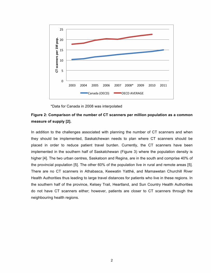
*Data for Canada in 2008 was interpolated

Figure 2: Comparison of the number of CT scanners per million population as a common

measure of supply [2].

In addition to the challenges associated with planning the number of CT scanners and when

they should be implemented, Saskatchewan needs to plan where CT scanners should be

placed in order to reduce patient travel burden. Currently, the CT scanners have been

implemented in the southern half of Saskatchewan (Figure 3) where the population density is

higher [4]. The two urban centres, Saskatoon and Regina, are in the south and comprise 40% of

the provincial population [5]. The other 60% of the population live in rural and remote areas [5].

There are no CT scanners in Athabasca, Keewatin Yatthé, and Mamawetan Churchill River

Health Authorities thus leading to large travel distances for patients who live in these regions. In

the southern half of the province, Kelsey Trail, Heartland, and Sun Country Health Authorities

do not have CT scanners either; however, patients are closer to CT scanners through the

neighbouring health regions.

0  

5  

10  

15  

20  

25  

2003   2004   2005   2006   2007   2008*   2009   2010   2011  

CT  sc

anne

rs  per  1M  pop

.  

Canada  (OECD)   OECD  AVERAGE  

3

Figure 3: Map of all Saskatchewan health regions with the CT scanner locations marked

by the city they are in and the number of CT scanners in brackets. [4]

To reduce the inequities in access while balancing supply and demand, this thesis will propose

a capacity planning model and use the province of Saskatchewan as a case study. This will aid

policy makers in knowing when and where CT scanners should be implemented. Although the

thesis is focused on Saskatchewan, we expect the work to be widely applicable for CT capacity

planning.

1.1. Contributions

There are three main areas of contribution from this thesis.

First, utilization and access metrics are presented based on data from all CT-equipped health

regions in Saskatchewan to understand the current situation. While previous papers have

discussed utilization and access in the United States, Norway, and Canada, this is the first

4

analysis for Saskatchewan. The key metrics are the number of exams per operating hour,

number of exams per 1000 population, and patient travel time.

Second, the capacity planning model is a mixed-integer optimization model. It is based on

choosing appropriate CT facilities to achieve patient access standards and understanding how

much regular operating capacity is needed at each facility. Saskatchewan’s utilization metrics

are used to estimate the parameters for the model.

Third, recommendations for capacity planning in Saskatchewan are discussed based on the

model results.

1.2. Organization

This thesis is organized as follows.

Chapter 2 reviews the literature relevant to CT scanner utilization and access to health care

services with a focus on geographic variations between urban and rural populations. For

capacity planning, it describes possible approaches from geography and operations research to

capacity planning for minimizing cost and travel burden. Chapter 3 presents the methods and

data used to understand the current CT scanner situation in Saskatchewan and to develop the

capacity planning model. Chapter 4 shows the results of the current situation in Saskatchewan

with respect to CT scanner utilization and access. Chapter 5 describes the capacity planning

model design and results. The design of the model and the scenarios are outlined in detail. The

aim is to understand the trade-offs between access and cost as well as the capacity necessary

to meet the demand in Saskatchewan. Chapter 6 presents practical recommendations and

ideas for future work.

5

Chapter 2. Literature Review

This chapter provides an overview of the existing trends in computed tomography utilization and

access as well as different types of capacity planning models.

2.1. CT Utilization and Access This section reviews the literature related trends in CT scanner usage in different jurisdictions

and the factors that affect access. This understanding feeds into CT scanner capacity planning.

2.1.1. Trends in Computed Tomography Usage

The motivation behind this research lies in the recent trends in diagnostic CT scanning in terms

of increases in supply, and utilization.

CT utilization is commonly measured by number of exams per a given population or percentage

of the population that have had a CT exam. Specific populations have been analyzed such as

inpatient, outpatient, emergency department patients [6], Medicare [7, 8], and health system

enrollees [9]. From the OECD Health Data in 2011 [2], Canadians receive 127 CT exams per

thousand population which is almost equal the OECD average of 127.9. In the United States,

there are many methods of calculating patient utilization based on specific populations including

enrollees [10], Medicare beneficiaries [7, 8], and case-mix adjusted patient admissions [11, 12].

This led to a large range in CT utilization values; however, the overall trend was that utilization

had increased over the past decade and that there was substantial regional variation. Due to the

healthcare funding models in the USA, each study focuses separately on a particular population

within the country and it is difficult to obtain data for the entire country, which also makes

international comparisons challenging. The USA has a high prevalence of self-referral, which is

when a physician refers a patient to a CT facility where they receive financial compensation

[13]. It is also common to have an additional technical fee, which is paid to the health facility

where the CT scanner is located [14]. Both the self-referral and technical fee change the

incentives for CT supply and utilization in the USA [13, 14]. Furthermore, physicians who refer

patients to physicians of the same specialty for diagnostic imaging, tend to use diagnostic

imaging more frequently than physicians who refer to radiologists [15].

Utilization has also been analyzed based on body region [8,15,16] but different categorizations

of body regions make it difficult to compare. In 2007, Parker et al. [8] analyzed the national

Medicare data in the USA and the most common CT exams by body region in descending order

6

were CT body, spine, head, musculoskeletal, vascular, and cardiac. Lee et al. [15] also

analyzed data from 2001 to 2007 for an adult emergency department at an urban academic

hospital in New York City. They found that out of all CT scans, 56% were head scans and 28%

were abdomen/pelvis scans. Although there were low percentages of chest (4%) and neck (8%)

scans overall, they had the largest increase of 600% and 500% respectively from 2001 to 2007.

Similarly in Korea, Oh et al. [16] analyzed data from 2001 to 2010 and the body regions with the

most exams were head (67.5%), abdomen (14.8%), chest (8.1%), and facial bones (6.6%),

miscellaneous CTs (2.4%) and cervical CTs (0.6%).

CT supply can be compared using number of CT scanners per million population. In the 2011

OECD Health Data [2], Canada was below the OECD average (23.2/million population) with

14.6 CT scanners per million population. In comparison, the supply ranged from 8.9 (United

Kingdom) to 50.6 (Australia). Taiwan had 3.71 per million population in 2001 [9].

For CT utilization and workload, the Canadian Institute for Health Information (CIHI) [1]

analyzed the number of exams per scanner per year and number of operating hours per

scanner per week in 2007. Facilities submit their data online and follow Management

Information System Standards. Compared with several European countries and the United

States, Canada’s CT utilization level is higher using the measure of exams per scanner per year

at 8,735, but the average number of exams and average number of hours in operation per CT

scanner suggests that CT scanners are underutilized [1]. On average, Saskatchewan’s CT

facilities operate 59 hours per week compared to the national average of 60 hours per week,

indicating that there may be an opportunity to increase utilization. However, several factors

need to be taken into consideration such as funding level, staff availability, and population

density [1].

When CIHI [17] released data from 2011-2012, Saskatchewan was above the national average

with 144.9 CT exams per thousand population and 15 CT scanners per million population.

When one looks at provincial statistics, there are substantial variations due to factors such as

population density, so the average national statistic can be misleading. The next section will

discuss geographic variations in CT utilization, supply, and access.

7

2.1.2. Geographic Variation and Access issues

While country comparisons are useful, there can also be substantial variations in utilization

between different regions within a country. This may be due to varying levels of CT accessibility

in each region.

Healthcare Access in General

An American survey in North Carolina revealed that the key determinant of health service

utilization is access to transportation resources such as a family member with a driver’s license

and car [18]. For mental health services, the more severe the diagnosis, the farther people were

willing to travel [19]. Nemet and Bailey [20] wrote that for the elderly, service utilization is also

dependent on where their other activities occur such as grocery shopping. These areas are

called their activity spaces. The closer the service is to their activity spaces, the higher the rates

of service utilization.

A study on USA Medicare claims data in 2008 [21] was adjusted for health status and found no

significant difference between urban and rural service utilization despite differences between

states. However, in another study, several states were selected in 1998 [22] and when their

claims data were analyzed, the population was stratified into urban, large rural, small rural, and

isolated rural populations. It showed that for general services, the travel burden difference

between urban and rural populations was not large, but was significant for specialized services.

Access in Radiology

Radiology studies in the USA [8, 23, 24] and Norway [25] show substantial geographic variation

in utilization and access to imaging services. While the American studies [8, 23, 24] noted that

there were differences between regions, the reasons for this variation were unknown. The

Norwegian study [25] ran correlations between radiological services, examinations rates, and

population and their differences were statistically significant between regions. However, when

the main urban centre, Oslo, was removed, the correlation was not significant between the non-

urban regions. The researchers found that accessibility was the main cause for variation

between populations and also found that socioeconomic factors, mainly education, led to

increased examination rates. Oslo had the highest education levels in Norway and had access

to private clinics. People with high education levels were more likely to pressure their physicians

8

for a referral. If physicians did not think the CT exam was medically necessary, they would refer

the patient to a private clinic instead of a publicly funded hospital.

In 2001, a Taiwanese study [9] analyzed national claims data from the universal and

comprehensive health insurance and found that increased CT utilization was correlated with the

percentage of females in the population, number of hospital physicians, and percentage of

children in the population. In general, females cost the healthcare system more and hospital

physicians drive healthcare costs. Children would receive more scans due to the disease

patterns in children and the population was more willing to spend healthcare resources on

children than elderly people. The percentage of elderly and income levels in Taiwan did not

correlate with increased utilization.

Access in Ontario

The Institute for Clinical Evaluative Studies (ICES) [26, 27] analyzed Ontario’s health insurance

claims for CT scans and found that CT scan rates increased 12% between 2003/2004 and

2004/2005. The replacement of old CT scanners with newer and faster machines was one

reason for the increase since more CT scans could potentially be done in the same amount of

time. When compared between Local Health Integration Networks (LHINs), the rural North

Simcoe Muskoka LHIN had the highest CT scanning rate which was 1.5 times higher than the

urban Hamilton Niagara Haldimand Brant LHIN with the lowest rate. Neighbourhood income did

not seem to have an impact on utilization rates. According to the ICES report in 2005, elderly

patients had higher rates of CT scanning and men aged 65 and older had higher scanning rates

than women in their age group. However, under age 65, men and women had similar CT

scanning rates.

While there has been a substantial amount of literature on CT utilization and health services

access in general, there has been no research that analyzes CT utilization, patient utilization,

and access to CT scanners in Saskatchewan.

9

2.2. Capacity Planning Methods Demand for CT exams is rising and reducing patient travel distance is important for service

access. Therefore, capacity planning for CT scanners in Saskatchewan needs to take the

following factors into consideration:

• Allowing multiple CT scanners at the same location

• Reducing patient travelling time to improve accessibility

• Minimizing the overall cost to the system

• Incorporating flexibility for different service levels (e.g. distances travelled, percentage of

demand serviced) since serving all patients equally may not be economically feasible

• Allowing a long planning horizon (e.g., 20 years) is useful for understanding how to

match demand as the population size and demography in each area changes.

To understand how these factors have been incorporated in the literature, this section will delve

into the capacity planning methods in medical imaging, geographical planning, and operations

research.

2.2.1. Capacity Planning in Medical Imaging

Although there have been many capacity planning models done in healthcare, few of them are

specific to medical imaging. Within medical imaging, there are general management articles

[27], heuristic methods [28], and a linear program [29] which consider patient travel times and

costs.

Szcepura and Clark [27] published a discussion on strategic management of magnetic

resonance imaging (MRI) in the United Kingdom’s National Health Service Trusts. While several

suggestions pertained to the organizational structure, their overall approach is to use population

projections and utilization rates to predict future demand. First, the total number of new MRIs

required for the United Kingdom was estimated. Although the exact estimation process is not

stated, the locations were then decided by the decision makers on the basis of patient travel

costs, equitable distribution of services, and gaining economies of scope. By tracking utilization

in each area over a period of time, they will assess when it will be appropriate to add a new MRI

and how the wait lists decrease in response. As wait lists decrease, they expect a slight

increase in MRI referrals, but are unsure of the relationship between waitlists and referrals. For

10

example, there could be a substantial jump in referrals if the waitlist drops to zero days.

Therefore, the implementation of MRIs will be an ongoing assessment based on utilization,

waitlists, and referrals.

In Germany, Bach and Hoberg [28] presented a model where combinations of alternative CT

scanner locations were chosen and then decision criteria were calculated such as total cost,

patient transportation cost, utilization level, maximum distance travelled, and number of CT

scanners implemented. By recognizing fixed threshold costs after a certain threshold capacity, a

second shift of staff would need to be employed to increase the capacity of the scanner.

Although it was presented in a similar manner to a linear program, they believe it is a more

practical approach for decision makers to look at various CT facility combinations and then

make a decision based on the differences in decision criteria results. From the results of the

alternatives, they developed a sequential process to add new CT scanners.

Greenwald et al [29] developed a static linear programming model for a 10-year planning

horizon to minimize CT facility costs, transportation costs, and opportunity costs of patient travel

times subject to capacity constraints and to satisfy all of the expected demand. The paper

focuses on patient travel cost estimates and opportunity costs by including hospital shuttle

costs, public transit, and wages lost due to time away from work. Assumptions of utilization level

and transportation costs were varied and the decision maker could choose the option given the

factors which were most important to them.

2.2.2. Geographical Methods

Geographical methods have also been used to estimate travel time and aid in capacity planning.

They incorporate road network usage and travel time estimates based on road speed limits. The

common software is ArcGIS for calculations and visual representation.

In Chicago [30], Wang and Luo calculated spatial accessibility for primary care physicians using

a two-step floating catchment area based on a threshold travel time between the population and

physicians. In rural British Columbia [31], hospital catchment areas were analyzed to look at the

percentage of the population they could serve within different travel times. For example, the

percentage of the rural population that can access the service within 15 minutes, 30 minutes,

and an hour. What-if scenarios allowed the policy maker to see the impact on the population

11

when a service is removed since it means that a certain percentage of the population may have

to travel four hours instead of two hours.

2.2.3. Facility Location Modelling in Operations Research

The concept of ensuring demand can be serviced while minimizing cost and improving access

has been approached from several different objectives.

• Minimize distance travelled by customers

• Minimize number of facilities

• Minimize total cost

Minimizing distance travelled or the number of facilities available is often used as a proxy for

minimizing cost and covering models are used especially for public services [32]. Location-

allocation and plant location problem models are used for the private sector since their objective

is to minimize total costs [32].

In covering models [33, 34], the three main types are set covering, p-median, and maximum

covering. In the set covering location problem, the total number of facilities assigned is

minimized to reduce cost. In p-median, the travel distance to the closest facility is minimized to

improve access by giving a specified number of new facilities to control cost. Similarly, the

maximum covering location problem sets a maximum travel distance allowed and locates a

specified number of facilities such that the most demand possible is within the maximum travel

distance.

For emergency services, Toregas et al. [35] used simple set covering and p-median models.

The simple covering models have also been built into a decision support tool in India for

neighbourhood planning of public services such as schools and health centres [36]. The models

have been expanded to take facility capacity into consideration with both maximum coverage

and partial coverage. The maximum coverage model views demand beyond a threshold

distance is not covered. For partial coverage, there is the first zone with full coverage and a

second threshold distance. Demand is partially covered if it is between the first zone and the

second threshold distance. This allows for a demand assignment that is less desirable, but is

still acceptable to reduce the number of facilities required. Distance is often used as a proxy for

12

time. This has been applied to locating shelters in preparation for disasters [37]. Storage

location modelling for emergency response used threshold travel time instead of distance and

each facility had different capacity levels [38].

Dynamic covering models have been used for long term planning [39]. A dynamic maximum

covering location problem was used for emergency services with multiple objectives [40]. A

stochastic model was developed with weighted scenarios, a specified number of facilities, and a

budget constraint. To locate medical services for large scale emergencies [41], a minimum

number of facilities were assigned to large demand points to ensure a minimum level of

coverage and scenarios were given different weights. The problem was solved with several

models including the maximum covering location problem, p-median, and p-centre model. The

p-centre model minimizes the maximum travel distance.

In location-allocation models and the plant location problem, the goal is to minimize the total

cost to meet all the demand [42]. For location-allocation models, there are fixed facility costs,

assignment costs, and variable costs [42]. For the plant location problem, the cost elements are

similar except that the assignment cost is generally a transportation cost [43]. There have also

been dynamic location problems which minimize total costs over a planning horizon [42].

Wesolowsky and Truscott [44] proposed the dynamic location-allocation problem which

minimized total costs including assignment costs and relocation costs over a planning horizon. It

has also been expanded to include minimum and maximum capacities to ensure manufacturing

efficiency and all demand must be satisfied. Decision rules for small scale public facilities have

also been derived using the location-allocation model [45]. For daycares [46], the location-

allocation algorithm was applied to maximize the number of people who can access the day

care within a threshold distance. A maximum travel restriction was placed with a decay function

since fewer people were expected to use the day care the farther they needed to travel.

Other facility location models have been developed for similar facility types including goal

programming and fuzzy goals. For locating plants while taking employee needs into

consideration [47], a goal programming model was developed to incorporate cost, air quality,

and quality of life. Quality of life included education, health, and community planning scores

which were out of 100. Capacity planning for libraries [48] in the Columbus, Ohio area was used

as a case study for a multi-objective dynamic location model with a fuzzy goal to take social

factors into consideration. The objective was to minimize the maximum deviation from the fuzzy

goal subject to budget constraints and accessibility measures (e.g. highway access, public

transportation, parking lots). Luss [49] wrote a large overview of capacity expansion problems in

13

operations research, including continuous and discrete models. While many papers looked at

continuous expansion sizes or discrete incrementing capacity sizes, having multiple facilities at

the same site had not been well explored.

Multiple facilities at the same site

Despite the substantial amount of research on facility location modelling, capacity planning

models to address our problem with multiple facilities at the same site are not well researched.

ReVelle and Laporte [43] identified this gap in the literature and proposed a static formulation for

the single product capacitated machine siting problem. It minimized total costs for new sites,

new machines at each site, product delivery, and product manufacturing. All demand had to be

satisfied and there were no delivery time or distance limitations.

Several papers had a p-median formulation based on having multiple facilities in each area and

then the model was re-run for each area [50 - 52]. Each area had a maximum number of

facilities it could implement to control costs. In this situation, the borders of each area were strict

– demand could only be fulfilled by a facility in its area. This was applied to electoral polling

stations in Italy [51].

The static capacitated facility location problem was expanded to include multiple facilities of

different types at each site [53]. Set-up costs were divided into opening the site and

implementing new facilities at the site. Like the plant location problem, a lower connection cost

was used to help assign demand to the appropriate facility. However, there were no delivery

time or distance limitations.

While the studies mentioned above include relevant pieces, our problem is not completely

represented by any of them.

14

Chapter 3. Methods

To develop a capacity planning model, an understanding of the current situation in

Saskatchewan with respect to CT utilization and access is needed. The province was used as a

case study. The three main stages are:

1. Data Acquisition and Processing

2. Metrics and Current Situation

3. Capacity Planning Model

The collected data were obtained from various sources. Metrics were calculated to extract a

better understanding of the current situation. Different scenarios were run on an optimization

model to illustrate a method for capacity planning, using the metrics to inform the model

parameters.

3.1. Data Acquisition and Processing

Data were obtained from the Regional Health Authorities (RHA), CT facilities, Statistics Canada,

and Saskatchewan’s Ministry of Health.

3.1.1. Regional Health Authorities

We requested anonymous patient-level data from each Regional Health Authority (RHA) with a

CT scanner for each CT exam for all the years within the Radiology Information System (RIS).

All RHAs provided data from different time periods as listed in Table 1 and common data fields

are listed in Table 2. To provide comparisons between RHAs, only complete years of data were

used starting in January. Although the data from each of the RHAs spans a few years, only

2011 data overlaps with all RHAs. This limited the analysis of the province since province-wide

exam data are not available for any other year.

15

Table 1: Date ranges and number of records for the exam-level data from RIS from each

health authority with a CT scanner.

Regional Health Authorities Data Date Range Number of Exams

Cypress 2007 November to 2013 April 21,976

Prince Albert Parkland 2010 April to 2013 December 41,531

Prairie North

2009 February to 2013 March

BUH: 2009 February to 2013 March

LH: 2009 April to 2013 March

34,497 total

BUH: 18,591

LH: 15,906

Sunrise 2010 November to 2013 October 15,883

Five Hills 2009 November to 2013 April 21,272

Saskatoon

2000 January to 2012 May

RUH – 2000 January to 2012 May

SPH – 2004 February to 2012 May

SCH – 2003 November to 2012 May

355,418 total

RUH: 184,643

SPH: 87,121

SCH: 83,654

Regina Qu’Appelle

2003 April to 2012 September

RGH – 2003 April to 2012 September

Pasqua – 2003 April to 2012 March

119,210 total

RGH: 97,472

Pasqua: 21,738

Table 2: Common RIS data fields for retrospective exam-level data from each health

authority.

Patient Data Imaging Data

Anonymous patient identifier/ visit identifier

Age

Sex

Postal Code

Patient Type (outpatient, inpatient, emergency)

Hospital/Facility

Exam date

Final report date (All except RQHR)

Order procedure

For the data fields provided by each RHA, see Appendix A

16

Due to different RIS programs, there are inconsistencies in how CT exams are recorded. For

example, RQHR records some emergency patients as inpatients. Order procedure and patient

type were re-categorized to make the data more consistent. Even among facilities with the same

RIS program there may be slight differences in how each staff member enters the information.

Furthermore, the dataset includes false starts and cancelled exams. The inconsistencies

negatively impact the quality of the data; however, the results will still provide a good

understanding of the general situation.

Order Procedure to Procedure group

All RHAs provided order procedure names indicating what type of CT exam was performed on

the patient which included details such as body location and whether contrast was used.

Procedure groups were based on body location (head, spine, thorax, abdomen/pelvis, lower

extremities, upper extremities, vascular, and miscellaneous). In total, there were 508 different

order procedures which were matched to the eight procedure groups. If an order procedure

contained multiple body locations then it was matched with multiple procedure groups.

Patient Type

Patient type (emergency, inpatient, outpatient) was recorded differently in each RHA’s dataset.

For each RHA, the different descriptors for patient type were matched as emergency, inpatient,

or outpatient. For example, “Orthopaedic Clinic” in Cypress RHA was re-categorized as

outpatient.

Cost Data

Saskatoon Health Region provided cost data from April 2011 to March 2013 with categories

such as salaries, drugs, and supplies. This allowed us to calculate an estimated cost per exam.

17

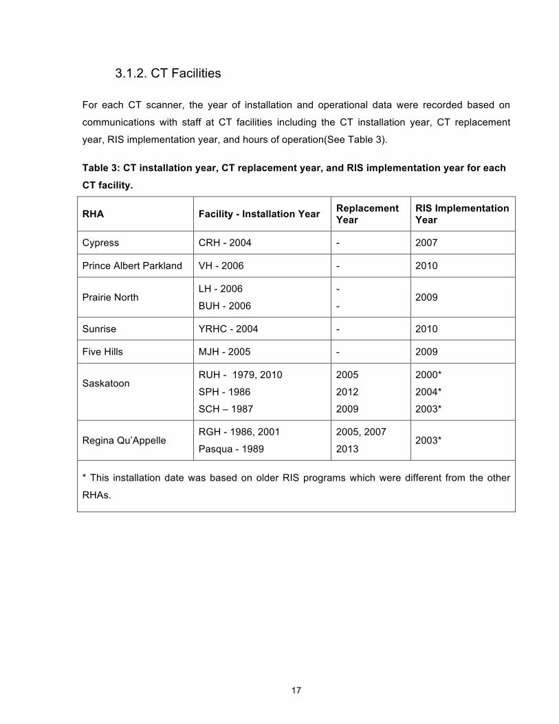
3.1.2. CT Facilities

For each CT scanner, the year of installation and operational data were recorded based on

communications with staff at CT facilities including the CT installation year, CT replacement

year, RIS implementation year, and hours of operation(See Table 3).

Table 3: CT installation year, CT replacement year, and RIS implementation year for each

CT facility.

RHA Facility - Installation Year Replacement Year

RIS Implementation Year

Cypress CRH - 2004 - 2007

Prince Albert Parkland VH - 2006 - 2010

Prairie North LH - 2006

BUH - 2006

-

- 2009

Sunrise YRHC - 2004 - 2010

Five Hills MJH - 2005 - 2009

Saskatoon

RUH - 1979, 2010

SPH - 1986

SCH – 1987

2005

2012

2009

2000*

2004*

2003*

Regina Qu’Appelle RGH - 1986, 2001

Pasqua - 1989

2005, 2007

2013 2003*

* This installation date was based on older RIS programs which were different from the other

RHAs.

18

3.1.3. Saskatchewan’s Ministry of Health

Saskatchewan’s Ministry of Health provided wait times by health region and data for emergency

and inpatients including those who did not receive a CT exam as outlined below.

Discharge Abstract Database (DAD)

The DAD provided general inpatient admissions and discharge data for all CT-equipped

hospitals from January 2000 to March 2013. Twelve years of data (2000 – 2012) were used in

the analysis since it was restricted to complete years of data. This decreases the seasonality

bias since each month was incorporated the same number of times. Data fields included were

admission date, sex, hospital, 5-year age cohorts, total length of stay, and unique patient

identifier. The unique patient identifier was a number assigned to a patient’s account and allows

multiple records to be linked to a patient while keeping the patient anonymous.

National Ambulatory Care Reporting System (NACRS)

NACRS provided emergency patient data for select hospitals from April 2011 to December 2012

(Table 4). This did not include all CT-equipped hospitals. Information was only provided for five

facilities because the data collection tool has not been implemented in the other CT facilities.

Data fields included were unique patient identifier, registration date, sex, hospital, 5-year age

cohorts, length of stay, and triage level.

Table 4: NACRS data date ranges by CT facility

CT Facility Data Date Range

RUH 2011 April to 2012 December

SPH 2011 April to 2012 December

SCH 2011 April to 2012 December

Pasqua 2012 April to 2012 September

RGH 2012 April to 2012 September

19

Wait Times

CT wait times as of December 31, 2011 were provided by the Ministry of Health and were

reported by priority level for each health region. Priority level is on a scale of 1 to 4 from

emergent to non-urgent. The wait time was defined as the number of days between the date a

CT facility receives the examination request and the date of the scheduled exam. There were

two methods for calculating wait time. Saskatoon and Regina Qu’Appelle Health Region used

the new reporting method which was based on days waited for exams which were completed.

The median and 90th percentile wait time in days was provided. The rest of the health regions

used an estimated maximum wait time based on the next available appointment in the schedule

and not the actual date of the scheduled exam.

3.1.4. Statistics Canada

Statistics Canada provides population and demographic data for census sub-divisions (CSD) as

well as population estimates and projections for the province. Furthermore, it provided the

postal code conversation file which links postal codes with CSDs.

Census 2011

From the national census in 2011, the population by age and sex was reported by CSD. Median

age and population density were additional fields.

National Household Survey 2011

From the National Household Survey in 2011, the data provided the size of the Aboriginal

population by CSD.

Population Estimates

The population of Saskatchewan was estimated from 2011 to 2014 to reflect the current

demographics by 5-year age cohorts and sex at the provincial level.

Population Projections

Statistics Canada publishes six scenarios for population projections [54]. They provided

provincial population projections by 5-year age cohorts and sex from 2014 to 2030 based on

provincial growth rates for the total population which assume medium growth and historical

migration trends (constant fertility rate of 1.7 births per woman, life expectancy of 80.4 years for

20

males and 87.3 years for females by 2036, constant national immigration rate of 0.75%, and

interprovincial migration rates based on 1981 to 2008). This set of growth assumptions is called

M1.

There were six possible scenarios; however, M1 was chosen out of four medium growth

scenarios since it was closest to the average in total population increase. Scenarios H and L for

high and low population growth respectively were also used to better understand the range of

population changes.

Postal Code Conversion File

The postal code conversion file [55] allows for matching between postal codes and Statistics

Canada administrative areas (e.g. dissemination areas, census sub-divisions, etc.). Additional

fields include the population centre and rural area classification and the latitude/longitude

coordinates for the CSD. The population centre and rural area classification distinguish between

urban and rural CSDs by population size. The latitude and longitude coordinates are based on

each CSD’s representative point which is weighted by the number of households.

Since postal codes can span multiple CSDs, a single link indicator provides a one-to-one match

between postal codes and dissemination areas based on the most number of households. An

example of how multiple CSDs and postal code borders do not align is in Figure 4. While the

single link indicator provided the most likely match, this can convert records from a postal code

to a CSD where the person does not live.

Figure 4: Boundaries of the One Arrow 95 CSD, neighbouring CSDs, and postal codes.

21

3.1.5. Key Calculations

Number of Exams

The number of exams is the number of times procedure groups are scanned in a visit. The

number of times an order procedure was executed in a visit is converted into the number of

procedure groups multiplied by the number of times it was executed. For example, if an order

procedure corresponded with two procedure groups and the order procedure was executed

twice, then this would count as four exams.

Travel Distance

The travel distance is the distance between a patient’s CSD (derived from their residential

postal code) to a CT facility. To calculate travel distance between a CSD and a CT facility, the

latitude and longitude coordinates of the representative point from the postal code conversion

file are converted into Universal Transverse Mercator (UTM) [56] in ArcGIS Desktop v10.2 [57].

UTM is a coordinate system based in metres. The Pythagoras Theorem is used to calculate the

rectilinear distance between a CSD’s representative point and a CT facility since this is a good

estimation of highway distances [58]

Travel Time

The travel time is the estimated driving time from the patient’s CSD centroid to CT facilities

using the road network. The ArcGIS’s Origin-Destination Cost Matrix tool in ArcGIS’s Network

Analyst toolbox was used to calculate the travel time using the road network from CanMap

RouteLogistics Saskatchewan v2013.3, population-weighted representative point coordinates,

and CT facility coordinates. The tool calculates the travel times by adding up the road segments

which create the shortest route and estimating times for each road segment using the posted

speed limits. If the representative point was farther than 5 km from the closest road segment,

ArcGIS could not calculate accurate travel times since the centroids were not close enough to

the road network. Thirteen of the CSDs had centroids where this was the case and their travel

times were estimated based on the rectilinear distance from the UTM coordinates for the

centroids and CT facilities. From there, the rectilinear distance was used to approximate travel

times assuming a speed of 100km/hour.

22

Matching Regional Health Authorities to Postal Codes

Using ArcGIS, the boundaries of postal codes and RHAs were matched to indicate which postal

codes overlapped the respective RHA. Postal codes could overlap with multiple RHAs and

contain many postal code areas. Since the number of postal code areas is based on the number

of addresses, it is an indication of population density. Therefore, the best match of a postal

code to a RHA is based on the highest number of postal code areas.

Populations Projections by Census Sub-Division until 2030

Saskatchewan’s population estimates and population projections were only provided at the

provincial level and not by CSD by 5-year age cohort and sex. To estimate population growth

each year at the provincial level, a year’s population is divided by last year’s population for each

20-year age cohort and sex at the provincial level. The 5-year age cohorts are combined to 20-

year age cohorts to match the 20-year age cohorts in the patient utilization data. For example, if

the population of female 0 to 19 year olds is 100 in 2011 and 150 in 2012, then the population

growth rate is 1.5. The population growth rates for each 20-year age cohort and sex and applied

to all CSDs each year until 2030 based on their 20-year age cohort and sex distribution in the

2011 census. For example, if the growth rate for 0 to 19 year olds is 1.5 in 2012, then a CSD

with 10 females aged 0 to 19 years old in 2011 would be calculated to have 15 people in that

population group. See Appendix B for population growth rates

23

3.2. Metrics and Current Situation

To understand the current situation with respect to CT scanners in Saskatchewan, metrics were

calculated to compare the different health regions and to estimate parameters for a capacity

planning model. The main dimensions for the metrics were CT provision, CT utilization, patient

utilization, and patient access. These calculations were performed in SPSS v.22. For simplicity,

it is assumed that all CT scanners can perform all exam types, although facilities have different

types of CT scanners depending on the physician specialists at the hospital. See Appendix C for

the number of records depending on how the data was segmented.

Due to the unavailability of critical data elements such as staffing levels and human resource

costs, not all desired metrics could be calculated. These include number of exams per human

resource working hour, number of CT operating hours per week per human resource type, cost

per exam, and cost per patient.

3.2.1. CT Provision

Understanding the amount of supply in a system is crucial. The two main metrics were the

number of CT scanners per million population and CT scanner operating hours per week.

Number of CT scanners per million population

The number of CT scanners in Saskatchewan was divided by the provincial population. This

allowed Saskatchewan to be compared to jurisdictions internationally.

𝑁𝑢𝑚𝑏𝑒𝑟  𝑜𝑓  𝐶𝑇  𝑠𝑐𝑎𝑛𝑛𝑒𝑟𝑠  𝑝𝑒𝑟  𝑚𝑖𝑙𝑙𝑖𝑜𝑛  𝑝𝑜𝑝𝑢𝑙𝑎𝑡𝑖𝑜𝑛 =  𝑁𝑢𝑚𝑏𝑒𝑟  𝑜𝑓  𝐶𝑇  𝑠𝑐𝑎𝑛𝑛𝑒𝑟𝑠  𝑖𝑛  𝑝𝑟𝑜𝑣𝑖𝑛𝑐𝑒

𝑝𝑟𝑜𝑣𝑖𝑛𝑐𝑖𝑎𝑙  𝑝𝑜𝑝𝑢𝑙𝑎𝑡𝑖𝑜𝑛∗ 1𝑀

CT scanner operating hours per week

Within each CT facility, CT scanners require specially trained staff who are available during

operating hours. By increasing the number of hours per week, the CT scanner should be able to

perform more exams thereby increasing capacity in the system.

24

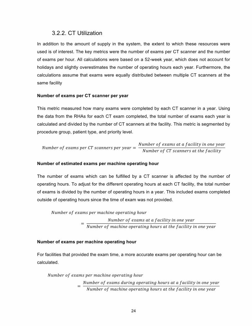
3.2.2. CT Utilization

In addition to the amount of supply in the system, the extent to which these resources were

used is of interest. The key metrics were the number of exams per CT scanner and the number

of exams per hour. All calculations were based on a 52-week year, which does not account for

holidays and slightly overestimates the number of operating hours each year. Furthermore, the

calculations assume that exams were equally distributed between multiple CT scanners at the

same facility

Number of exams per CT scanner per year

This metric measured how many exams were completed by each CT scanner in a year. Using

the data from the RHAs for each CT exam completed, the total number of exams each year is

calculated and divided by the number of CT scanners at the facility. This metric is segmented by

procedure group, patient type, and priority level.

𝑁𝑢𝑚𝑏𝑒𝑟  𝑜𝑓  𝑒𝑥𝑎𝑚𝑠  𝑝𝑒𝑟  𝐶𝑇  𝑠𝑐𝑎𝑛𝑛𝑒𝑟𝑠  𝑝𝑒𝑟  𝑦𝑒𝑎𝑟 =  𝑁𝑢𝑚𝑏𝑒𝑟  𝑜𝑓  𝑒𝑥𝑎𝑚𝑠  𝑎𝑡  𝑎  𝑓𝑎𝑐𝑖𝑙𝑖𝑡𝑦  𝑖𝑛  𝑜𝑛𝑒  𝑦𝑒𝑎𝑟𝑁𝑢𝑚𝑏𝑒𝑟  𝑜𝑓  𝐶𝑇  𝑠𝑐𝑎𝑛𝑛𝑒𝑟𝑠  𝑎𝑡  𝑡ℎ𝑒  𝑓𝑎𝑐𝑖𝑙𝑖𝑡𝑦

Number of estimated exams per machine operating hour

The number of exams which can be fulfilled by a CT scanner is affected by the number of

operating hours. To adjust for the different operating hours at each CT facility, the total number

of exams is divided by the number of operating hours in a year. This included exams completed

outside of operating hours since the time of exam was not provided.

𝑁𝑢𝑚𝑏𝑒𝑟  𝑜𝑓  𝑒𝑥𝑎𝑚𝑠  𝑝𝑒𝑟  𝑚𝑎𝑐ℎ𝑖𝑛𝑒  𝑜𝑝𝑒𝑟𝑎𝑡𝑖𝑛𝑔  ℎ𝑜𝑢𝑟

=  𝑁𝑢𝑚𝑏𝑒𝑟  𝑜𝑓  𝑒𝑥𝑎𝑚𝑠  𝑎𝑡  𝑎  𝑓𝑎𝑐𝑖𝑙𝑖𝑡𝑦  𝑖𝑛  𝑜𝑛𝑒  𝑦𝑒𝑎𝑟

𝑁𝑢𝑚𝑏𝑒𝑟  𝑜𝑓  𝑚𝑎𝑐ℎ𝑖𝑛𝑒  𝑜𝑝𝑒𝑟𝑎𝑡𝑖𝑛𝑔  ℎ𝑜𝑢𝑟𝑠  𝑎𝑡  𝑡ℎ𝑒  𝑓𝑎𝑐𝑖𝑙𝑖𝑡𝑦  𝑖𝑛  𝑜𝑛𝑒  𝑦𝑒𝑎𝑟

Number of exams per machine operating hour

For facilities that provided the exam time, a more accurate exams per operating hour can be

calculated.

𝑁𝑢𝑚𝑏𝑒𝑟  𝑜𝑓  𝑒𝑥𝑎𝑚𝑠  𝑝𝑒𝑟  𝑚𝑎𝑐ℎ𝑖𝑛𝑒  𝑜𝑝𝑒𝑟𝑎𝑡𝑖𝑛𝑔  ℎ𝑜𝑢𝑟

=  𝑁𝑢𝑚𝑏𝑒𝑟  𝑜𝑓  𝑒𝑥𝑎𝑚𝑠  𝑑𝑢𝑟𝑖𝑛𝑔  𝑜𝑝𝑒𝑟𝑎𝑡𝑖𝑛𝑔  ℎ𝑜𝑢𝑟𝑠  𝑎𝑡  𝑎  𝑓𝑎𝑐𝑖𝑙𝑖𝑡𝑦  𝑖𝑛  𝑜𝑛𝑒  𝑦𝑒𝑎𝑟𝑁𝑢𝑚𝑏𝑒𝑟  𝑜𝑓  𝑚𝑎𝑐ℎ𝑖𝑛𝑒  𝑜𝑝𝑒𝑟𝑎𝑡𝑖𝑛𝑔  ℎ𝑜𝑢𝑟𝑠  𝑎𝑡  𝑡ℎ𝑒  𝑓𝑎𝑐𝑖𝑙𝑖𝑡𝑦  𝑖𝑛  𝑜𝑛𝑒  𝑦𝑒𝑎𝑟

25

3.2.3. Patient Utilization

To understand where current utilization was coming from, patient utilization was analyzed in

terms of the general population, inpatient population, and emergency patients.

Number of exams per 1000 population per year

Using the exam data from RHAs the patient’s postal code was matched to a CSD with Statistics

Canada’s Postal Code Conversation File. The number of exams completed on patients from

each CSD was divided by the population of the CSD in order to understand the variability in

utilization among CSDs. It was also calculated by 20-year age cohorts and sex. Due to the

limitations of the single link indicator in the Postal Code Conversion File, some CSDs will have

more exams attributed to them than in actuality and some will have less.

𝑁𝑢𝑚𝑏𝑒𝑟  𝑜𝑓  𝑒𝑥𝑎𝑚𝑠  𝑝𝑒𝑟  1000  𝑝𝑜𝑝𝑢𝑙𝑎𝑡𝑖𝑜𝑛  𝑝𝑒𝑟  𝑦𝑒𝑎𝑟

=  𝑁𝑢𝑚𝑏𝑒𝑟  𝑜𝑓  𝑒𝑥𝑎𝑚𝑠    𝑝𝑒𝑟𝑓𝑜𝑟𝑚𝑒𝑑  𝑜𝑛  𝑝𝑎𝑡𝑖𝑒𝑛𝑡𝑠  𝑓𝑟𝑜𝑚  𝑡ℎ𝑎𝑡  𝑎𝑟𝑒𝑎  𝑖𝑛  𝑜𝑛𝑒  𝑦𝑒𝑎𝑟

𝑃𝑜𝑝𝑢𝑙𝑎𝑡𝑖𝑜𝑛  𝑜𝑓  𝑡ℎ𝑎𝑡  𝑎𝑟𝑒𝑎∗ 1000

Number of exams per 1000 inpatient visits per year

The number of inpatient exams from RHA data was divided by the number of inpatients at each

CT-equipped hospital from the DAD. This provided a better understanding of how inpatients use

CT scanners at different rates than the general population and between different CT facilities.

𝑁𝑢𝑚𝑏𝑒𝑟  𝑜𝑓  𝑒𝑥𝑎𝑚𝑠  𝑝𝑒𝑟  1000  𝑖𝑛𝑝𝑎𝑡𝑖𝑒𝑛𝑡𝑠  𝑝𝑒𝑟  𝑦𝑒𝑎𝑟

=  𝑁𝑢𝑚𝑏𝑒𝑟  𝑜𝑓  𝑒𝑥𝑎𝑚𝑠    𝑝𝑒𝑟𝑓𝑜𝑟𝑚𝑒𝑑  𝑜𝑛  𝑖𝑛𝑝𝑎𝑡𝑖𝑒𝑛𝑡𝑠    𝑖𝑛  𝑜𝑛𝑒  𝑦𝑒𝑎𝑟

𝑁𝑢𝑚𝑏𝑒𝑟  𝑜𝑓  𝑖𝑛𝑝𝑎𝑡𝑖𝑒𝑛𝑡  𝑣𝑖𝑠𝑖𝑡𝑠  𝑖𝑛  𝑜𝑛𝑒  𝑦𝑒𝑎𝑟  ∗ 1000

Number of exams per 1000 emergency visits per year

The number of emergency exams from the RHA data was divided by the number of emergency

patients at certain hospitals from the NACRS. The aim was to understand the rate of utilization

by emergency patients. Data was taken from April 2011 to March 2012 for Saskatoon Health

Region.

𝑁𝑢𝑚𝑏𝑒𝑟  𝑜𝑓  𝑒𝑥𝑎𝑚𝑠  𝑝𝑒𝑟  1000  𝑒𝑚𝑒𝑟𝑔𝑒𝑛𝑐𝑦  𝑣𝑖𝑠𝑖𝑡𝑠  𝑝𝑒𝑟  𝑦𝑒𝑎𝑟

=  𝑁𝑢𝑚𝑏𝑒𝑟  𝑜𝑓  𝑒𝑥𝑎𝑚𝑠    𝑝𝑒𝑟𝑓𝑜𝑟𝑚𝑒𝑑  𝑜𝑛  𝑒𝑚𝑒𝑟𝑔𝑒𝑛𝑐𝑦  𝑝𝑎𝑡𝑖𝑒𝑛𝑡𝑠    𝑖𝑛  𝑜𝑛𝑒  𝑦𝑒𝑎𝑟

𝑁𝑢𝑚𝑏𝑒𝑟  𝑜𝑓  𝑒𝑚𝑒𝑟𝑔𝑒𝑛𝑐𝑦  𝑣𝑖𝑠𝑖𝑡𝑠  𝑖𝑛  𝑜𝑛𝑒  𝑦𝑒𝑎𝑟  ∗ 1000

26

3.2.4. Patient Access

One of the key factors in patient utilization is the ease of access. Access was measured by

patient travel distance, estimated travel time, wait time, and report turnaround time.

Rectilinear patient travel distance

As described in Section 0, the travel distance is the number of kilometers from the centroid of

the patient’s residential CSD to a CT facility where the exam was completed. The patient’s

residential CSD was determined from their postal code in the RHA data. To estimate the

distance travelled on the street grid, the rectilinear distance between the CSD’s centroid and CT

facility was used.

Wait times

Data from the RHA’s were insufficient for calculating wait time since the exam referral date was

not provided. Therefore, the publicly reported wait times were obtained from Saskatchewan’s

Ministry of Health. The wait time is defined as the number of days between the date a facility

receives the examination request and the date set for the scheduled exam.

3.2.5. Expected Demand

Provincial patient utilization rates (exams per 1000 population) from 2011 for 20-year age

cohorts and sex were multiplied by to the age cohort and sex distribution of each CSD in 2011

to calculate an expected demand for CT exams. This was calculated to visually identify the

difference between current utilization rates in a CSD and then adjust this for the demographics

in each CSD since there are potentially lower utilization rates in CSDs located farther from CT

facilities among other factors [19].

27

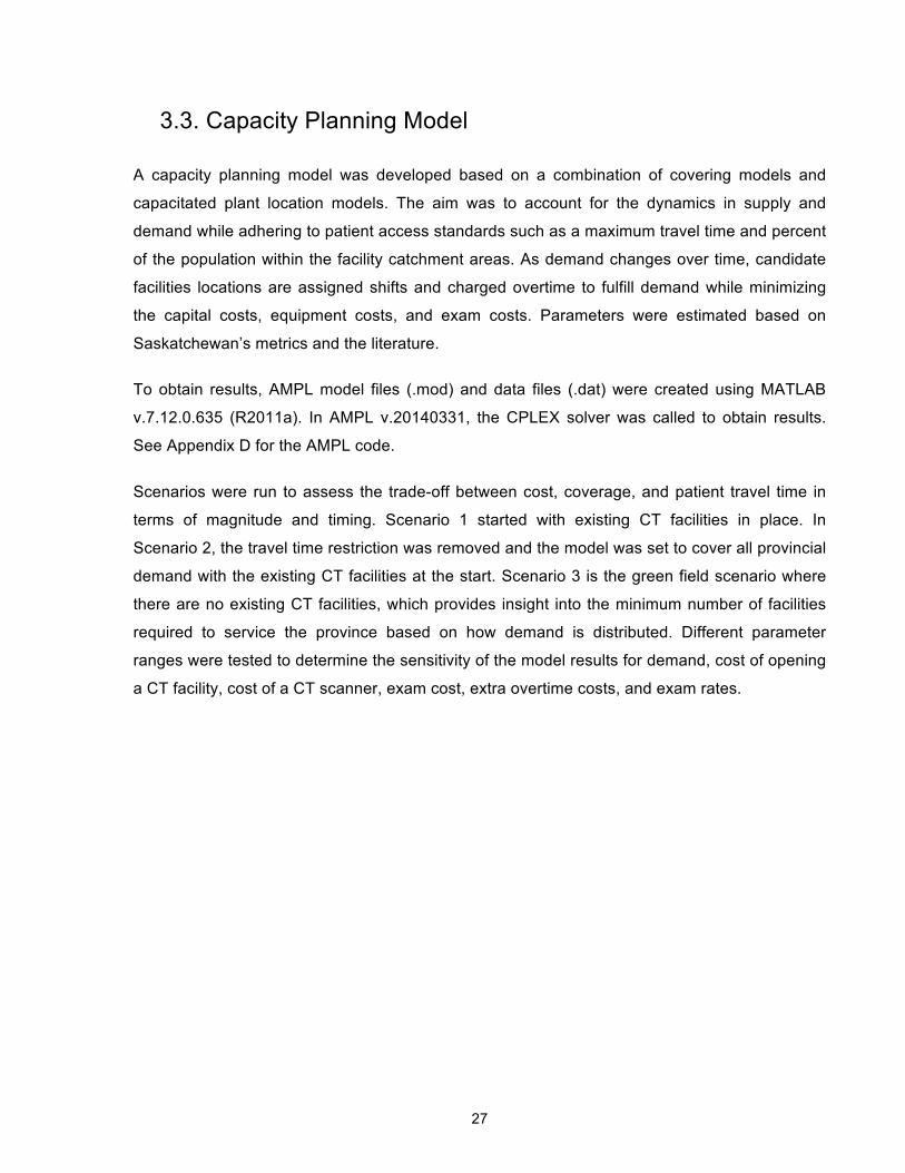
3.3. Capacity Planning Model

A capacity planning model was developed based on a combination of covering models and

capacitated plant location models. The aim was to account for the dynamics in supply and

demand while adhering to patient access standards such as a maximum travel time and percent

of the population within the facility catchment areas. As demand changes over time, candidate

facilities locations are assigned shifts and charged overtime to fulfill demand while minimizing

the capital costs, equipment costs, and exam costs. Parameters were estimated based on

Saskatchewan’s metrics and the literature.

To obtain results, AMPL model files (.mod) and data files (.dat) were created using MATLAB

v.7.12.0.635 (R2011a). In AMPL v.20140331, the CPLEX solver was called to obtain results.

See Appendix D for the AMPL code.

Scenarios were run to assess the trade-off between cost, coverage, and patient travel time in

terms of magnitude and timing. Scenario 1 started with existing CT facilities in place. In

Scenario 2, the travel time restriction was removed and the model was set to cover all provincial

demand with the existing CT facilities at the start. Scenario 3 is the green field scenario where

there are no existing CT facilities, which provides insight into the minimum number of facilities

required to service the province based on how demand is distributed. Different parameter

ranges were tested to determine the sensitivity of the model results for demand, cost of opening

a CT facility, cost of a CT scanner, exam cost, extra overtime costs, and exam rates.

28

Chapter 4. Current Situation of CT Utilization and Patient

Access in Saskatchewan

An analysis of the current situation was conducted by calculating metrics on current levels of CT

supply and patient utilization as well as the accessibility of the services. Supply is split into CT

provision and CT utilization. These metrics for CT provision are measures of the system’s

available capacity. For CT utilization, metrics provide a picture of how much output is produced

given the available capacity. Patient utilization provides an understanding of the utilization rate

variation between different geographic areas and hospitals in Saskatchewan based on the

patient’s residential postal code and provides insight into demand, albeit imperfectly as unmet

demand is not captured. The accessibility of services for patients is estimated through analysis

of patient travel distances to the CT facilities and overall statistics on where patients are

travelling. Understanding these factors can assist with interpreting results of the capacity

planning model and the limitations based on the estimation of parameters. Furthermore, using

calculated exam rates by age cohort and sex, an expected demand is calculated to identify

potential areas of unmet demand.

This chapter outlines the results for each metric and the expected demand calculation.

4.1. CT Provision

Saskatchewan has 13 CT scanners at 11 facilities. In Table 5, the number of CT scanners per

million population has increased substantially in the past ten years with a slight dip in 2011 due

to the increase in population. The number of CT scanners in the province has increased from

five to thirteen from 2001 to 2011. The census population has decreased slightly in 2006 and

then increased in 2011.

Table 5: Number of CTs per million population in Saskatchewan for each census year

Year Provincial Population

Number of CT scanners

CT per million population

2001 978,933 5 5.12

2006 968,157 12 12.39

2011 1,066,300 13 12.19

29

4.1.1. Operating Hours

Each CT facility has different weekly operating hours for each CT scanner, which are listed in

Table 6. The provincial average operating hours per CT scanner is 58.64 hours per week. For

CT facilities indicated with an asterisk in Table 6, the daily operating hours are an extra 30

minutes long. For example, Cypress Region Hospital starts at 7:30am instead of 8:00am and

runs for 8.5 hours per weekday instead of 8 hours per weekday. This allows for a bank day,

which is when the CT scanners are maintained for a day every three weeks.

Table 6: Operating Hours for each CT facility.

CT Facility (Region – Facility) Weekdays (Mon. - Fri.)

Weekends (Sat. - Sun.)

Average Hours/Wk

Cypress - Cypress Regional Hospital* 7:30 - 16:00 - 40

Five Hills - Moose Jaw Union Hospital* 8:00 - 16:30 - 40

Prince Albert Parkland - Victoria Hospital* 8:00 - 16:30 8:00 - 16:30** 40 or 54**

Prairie North - Battlefords Union Hospital* 8:00 - 16:30 - 40

Prairie North - Lloydminster Hospital* 8:00 - 16:30 - 40

Regina Qu'Appelle - Pasqua Hospital* 7:00 - 0:30 7:00 - 0:30 119

Regina Qu'Appelle - Regina General Hospital

CT 1: 7:00 - 23:00 CT 2: 7:00 - 17:00

CT 1: 7:00 - 23:00 CT 2: 7:00 - 17:00 182

Saskatoon - Royal University Hospital* CT 1: 9:30 - 16:00 CT 2: 7:30 - 22:30

CT 1: -- CT 2: 8:00 - 0:00 137

Saskatoon - Saskatoon City Hospital * 7:30 - 17:30 9:15 - 15:30 *** 62.5***

Saskatoon - St. Paul's Hospital* 7:30 - 17:00 - 50

Sunrise - Yorkton Regional Health Centre* 8:00 - 16:30 - 40

*There is an extra half hour in the schedule for “bank days”, so hours per week is the average

weekly hours including the bank days.

**These weekend operating hours started in January 2013 which increased the average hours

per week from 40 to 54.

***These weekend operating hours started in January 2010 and the average hours per week

include the weekend hours.

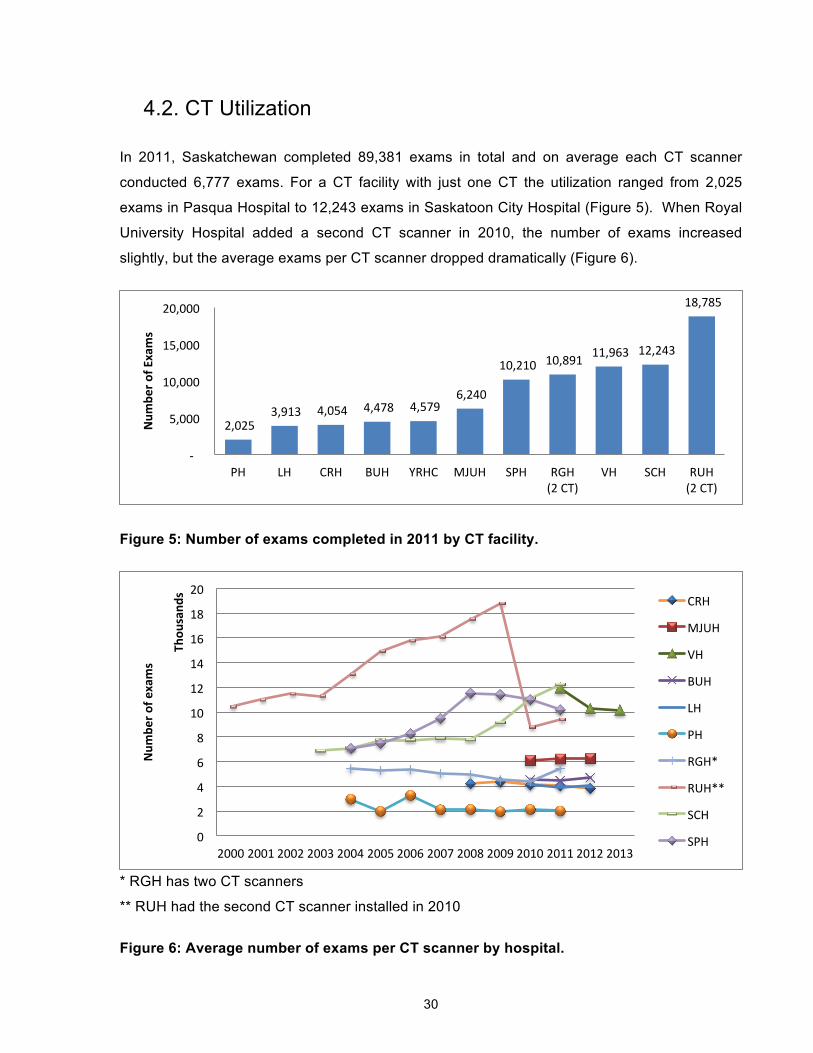
30

4.2. CT Utilization

In 2011, Saskatchewan completed 89,381 exams in total and on average each CT scanner

conducted 6,777 exams. For a CT facility with just one CT the utilization ranged from 2,025

exams in Pasqua Hospital to 12,243 exams in Saskatoon City Hospital (Figure 5). When Royal

University Hospital added a second CT scanner in 2010, the number of exams increased

slightly, but the average exams per CT scanner dropped dramatically (Figure 6).

Figure 5: Number of exams completed in 2011 by CT facility.

* RGH has two CT scanners

** RUH had the second CT scanner installed in 2010

Figure 6: Average number of exams per CT scanner by hospital.

 2,025      3,913      4,054      4,478      4,579    

 6,240    

 10,210      10,891      11,963      12,243    

 18,785    

 -­‐        

 5,000    

 10,000    

 15,000    

 20,000    

PH   LH   CRH   BUH   YRHC   MJUH   SPH   RGH          (2  CT)  

VH   SCH   RUH          (2  CT)  

Num

ber  o

f  Exams  

0  

2  

4  

6  

8  

10  

12  

14  

16  

18  

20  

2000  2001  2002  2003  2004  2005  2006  2007  2008  2009  2010  2011  2012  2013  

Num

ber  o

f  exams  

Thou

sand

s   CRH  

MJUH  

VH  

BUH  

LH  

PH  

RGH*  

RUH**  

SCH  

SPH  

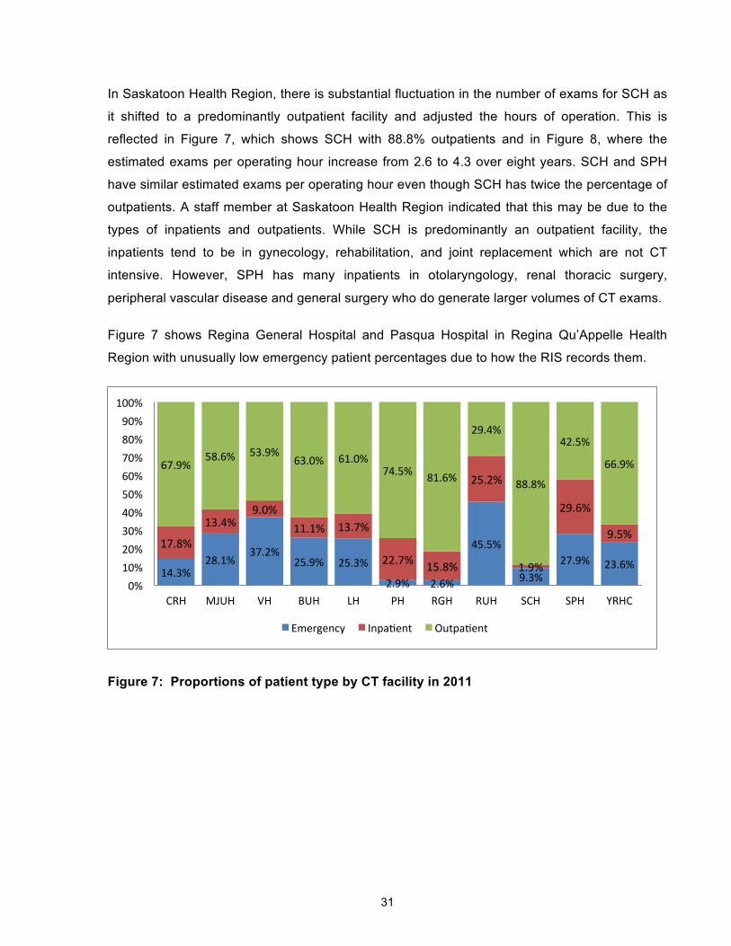
31

In Saskatoon Health Region, there is substantial fluctuation in the number of exams for SCH as

it shifted to a predominantly outpatient facility and adjusted the hours of operation. This is

reflected in Figure 7, which shows SCH with 88.8% outpatients and in Figure 8, where the

estimated exams per operating hour increase from 2.6 to 4.3 over eight years. SCH and SPH

have similar estimated exams per operating hour even though SCH has twice the percentage of

outpatients. A staff member at Saskatoon Health Region indicated that this may be due to the

types of inpatients and outpatients. While SCH is predominantly an outpatient facility, the

inpatients tend to be in gynecology, rehabilitation, and joint replacement which are not CT

intensive. However, SPH has many inpatients in otolaryngology, renal thoracic surgery,

peripheral vascular disease and general surgery who do generate larger volumes of CT exams.

Figure 7 shows Regina General Hospital and Pasqua Hospital in Regina Qu’Appelle Health

Region with unusually low emergency patient percentages due to how the RIS records them.

Figure 7: Proportions of patient type by CT facility in 2011

14.3%  28.1%  

37.2%  25.9%   25.3%  

2.9%   2.6%  

45.5%  

9.3%  27.9%   23.6%  

17.8%  

13.4%  9.0%  

11.1%   13.7%  

22.7%   15.8%  

25.2%  

1.9%  

29.6%  

9.5%  

67.9%  58.6%   53.9%  

63.0%   61.0%  74.5%   81.6%  

29.4%  

88.8%  

42.5%  

66.9%  

0%  10%  20%  30%  40%  50%  60%  70%  80%  90%  

100%  

CRH   MJUH   VH   BUH   LH   PH   RGH   RUH   SCH   SPH   YRHC  

Emergency   InpaQent   OutpaQent  

32

Figure 8: Estimated exams per operating hour by CT facility and year which includes on-

call exams.

The new RIS system records the time of the CT exam, which allows for the removal of exams

that occur outside the main operating hours. Most of the exams per operating hour ranged from

1.4 to 2.3 and remained stable (Figure 9). However, over three years Victoria Hospital in Prince

Albert Parkland Health Region the number of exams per operating hour decreased from 4.2 to

2.6. Part of this is due to increased operating hours in 2013. However, Victoria Hospital’s 2.6

exams per operating hour is still higher than the other CT facilities. When comparing the

difference between estimated exams per hour with the number of exams per hour, the average

difference is 0.74 exams more per hour. This makes sense since estimated exams per hour

includes exams completed outside of operating hours. However, the end time of the exam was

not known.

0  

1  

2  

3  

4  

5  

6  

2000   2001   2002   2003   2004   2005   2006   2007   2008   2009   2010   2011   2012   2013  

Es9m

ated

 num

ber  o

f  exm

as  

CRH  

MJUH  

VH  

BUH  

LH  

PH  

RGH  

RUH  

SCH  

SPH  

YRHC  

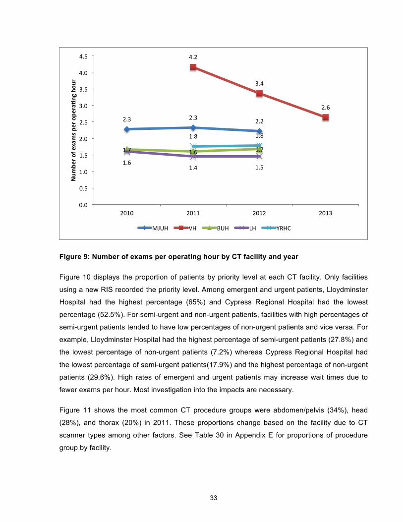
33

Figure 9: Number of exams per operating hour by CT facility and year

Figure 10 displays the proportion of patients by priority level at each CT facility. Only facilities

using a new RIS recorded the priority level. Among emergent and urgent patients, Lloydminster

Hospital had the highest percentage (65%) and Cypress Regional Hospital had the lowest

percentage (52.5%). For semi-urgent and non-urgent patients, facilities with high percentages of

semi-urgent patients tended to have low percentages of non-urgent patients and vice versa. For

example, Lloydminster Hospital had the highest percentage of semi-urgent patients (27.8%) and

the lowest percentage of non-urgent patients (7.2%) whereas Cypress Regional Hospital had

the lowest percentage of semi-urgent patients(17.9%) and the highest percentage of non-urgent

patients (29.6%). High rates of emergent and urgent patients may increase wait times due to

fewer exams per hour. Most investigation into the impacts are necessary.

Figure 11 shows the most common CT procedure groups were abdomen/pelvis (34%), head

(28%), and thorax (20%) in 2011. These proportions change based on the facility due to CT

scanner types among other factors. See Table 30 in Appendix E for proportions of procedure

group by facility.

2.3   2.3   2.2  

4.2  

3.4  

2.6  

1.7   1.6   1.7  

1.6  1.4   1.5  

1.8   1.8  

0.0  

0.5  

1.0  

1.5  

2.0  

2.5  

3.0  

3.5  

4.0  

4.5  

2010   2011   2012   2013  

Num

ber  o

f  exams  p

er  ope

ra9n

g  ho

ur  

MJUH   VH   BUH   LH   YRHC  

34

Figure 10: Proportion of patients by priority levels and CT facility in 2011.

Figure 11: Proportion of exams by procedure group in 2011.

4.3. Demographics

Saskatchewan has an insured population of 1,122,537 people and there were 78,687 in-

province CT patients in 2011. The insured population is the number of people which have a

current health card number in Saskatchewan and who therefore have health coverage. Figure

12 provides a breakdown of the size of the insured population for each health region. The

insured population is actually larger than the population of 1,066,300 people reported in the

2011 census by Statistics Canada. This is an ongoing trend due to fraud, death, and migration

outward among other possible factors. Every three years health cards are renewed and the

provincial health registry is updated. After the updates, the insured population more closely

matches Statistics Canada population estimates. [59]

34.5%   45.2%   47.3%  35.4%   36.3%   42.9%  

18.1%  12.9%   15.9%   28.3%   28.8%   19.9%  

17.9%  23.3%  

25.2%   26.4%   27.8%   22.5%  29.6%   18.6%   11.6%   9.9%   7.2%   14.7%  

0%  

20%  

40%  

60%  

80%  

100%  

CRH   MJUH   VH   BUH   LH   YRHC  

1  (Emergent)   2  (Urgent)   3  (Semi-­‐Urgent)   4  (Non-­‐Urgent)  

0.5%   1.4%   2.0%  6.4%   7.1%  

20.4%  28.4%  

33.8%  

0%  5%  

10%  15%  20%  25%  30%  35%  40%  

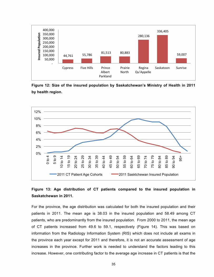
35

Figure 12: Size of the insured population by Saskatchewan’s Ministry of Health in 2011

by health region.

Figure 13: Age distribution of CT patients compared to the insured population in

Saskatchewan in 2011.

For the province, the age distribution was calculated for both the insured population and their

patients in 2011. The mean age is 38.03 in the insured population and 58.49 among CT

patients, who are predominantly from the insured population. From 2000 to 2011, the mean age

of CT patients increased from 49.6 to 59.1, respectively (Figure 14). This was based on

information from the Radiology Information System (RIS) which does not include all exams in

the province each year except for 2011 and therefore, it is not an accurate assessment of age

increases in the province. Further work is needed to understand the factors leading to this

increase. However, one contributing factor to the average age increase in CT patients is that the

 44,761      55,786      81,513      80,883    

 280,136      336,405    

 59,007    

 -­‐          50,000      100,000      150,000      200,000      250,000      300,000      350,000      400,000    

 Cypress      Five  Hills      Prince  Albert  

Parkland    

 Prairie  North    

 Regina  Qu’Appelle    

 Saskatoon      Sunrise    

Insured  Po

pula9o

n  

0%

2%

4%

6%

8%

10%

12%

0 to

4

5 to

9

10 to

14

15 to

19

20 to

24

25 to

29

30 to

34

35 to

39

40 to

44

45 to

49

50 to

54

55 to

59

60 to

64

65 to

69

70 to

74

75 to

79

80 to

84

85 to

89

90 to

94

95+

2011 CT Patient Age Cohorts 2011 Sasktchewan Insured Population

36

number of people aged 65 and older has increased substantially from 147,570 in 2001, to

216,160 in 2011 [60]. Since elderly patients have higher exam rates (Figure 18), this increases

the average age of CT patients. A higher average age could indicate an increase in the number

of exams needed for the province.

Between the health regions in 2011, Prairie North Health Region had the lowest mean patient

age of 55.5 year old and Sunrise Health Region had the oldest with a mean age of 62.9 years

old (Figure 15). In 2011, the sex distribution was 50.3% female and 49.7% male.

Figure 14: Mean CT patient age in Saskatchewan based on data from the RIS.

Figure 15: Mean CT patient age in 2011 for each health region.

49.6 50.3 50.5 53.5 56.5 56.9 57.1 57.3 57.5 57.6 57.9 58.5 59.1

0 10 20 30 40 50 60 70

2000 2001 2002 2003 2004 2005 2006 2007 2008 2009 2010 2011 2012

Year

Mea

n Pa

tient

Age

61 61.3 58.8 55.5 59.4 57.7 62.9

0 10 20 30 40 50 60 70

Cypress Five Hills Prince Albert Parkland

Prairie North Regina Qu’Appelle

Saskatoon Sunrise

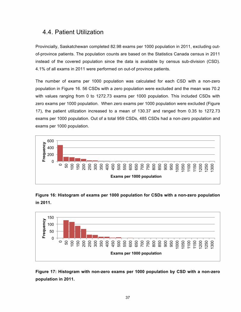
37

4.4. Patient Utilization

Provincially, Saskatchewan completed 82.98 exams per 1000 population in 2011, excluding out-

of-province patients. The population counts are based on the Statistics Canada census in 2011

instead of the covered population since the data is available by census sub-division (CSD).

4.1% of all exams in 2011 were performed on out-of province patients.

The number of exams per 1000 population was calculated for each CSD with a non-zero

population in Figure 16. 56 CSDs with a zero population were excluded and the mean was 70.2

with values ranging from 0 to 1272.73 exams per 1000 population. This included CSDs with

zero exams per 1000 population. When zero exams per 1000 population were excluded (Figure

17), the patient utilization increased to a mean of 130.37 and ranged from 0.35 to 1272.73

exams per 1000 population. Out of a total 959 CSDs, 485 CSDs had a non-zero population and

exams per 1000 population.

Figure 16: Histogram of exams per 1000 population for CSDs with a non-zero population

in 2011.

Figure 17: Histogram with non-zero exams per 1000 population by CSD with a non-zero

population in 2011.

0

200

400

600

0 50

100

150

200

250

300

350

400

450

500

550

600

650

700

750

800

850

900

950

1000

10

50

1100

11

50

1200

12

50

1300

Freq

uenc

y

Exams per 1000 population

0

50

100

150

0 50

100

150

200

250

300

350

400

450

500

550

600

650

700

750

800

850

900

950

1000

10

50

1100

11

50

1200

12

50

1300

Freq

uenc

y

Exams per 1000 population

38

Patient utilization rates were calculated by 20-year age cohorts and sex (Figure 18). Utilization

increased as patients became older, ranging from 11 to 235.8 exams per 1000 population for

females and 13.6 to 335.3 for males in 2011.

Figure 18: Number of exams per 1000 population by 20-year age cohorts and sex in 2011.

Patient utilization was also calculated for inpatients and emergency patients. Provincially,

inpatients had an imaging rate of 167.09 exams per 1000 inpatient visits in 2011 ranging from

43.79 to 319.85 in Saskatoon City Hospital and St. Paul’s Hospital respectively (Figure 19). The

factors which contribute to this difference are discussed in Section 4.2.

Figure 19: Exams per 1000 inpatient visits by facility

For emergency patients, the imaging rate from April 2011 to March 2012 was 156.71, 66.617,

and 69.541 exams per 1000 emergency visits for RUH, SCH, and SPH respectively. Emergency

imaging rates could not be calculated for other hospitals due to lack of data.

11.0  45.5  

93.0  

187.6  235.8  

13.6  46.0  

84.5  

272.0  335.3  

0  

100  

200  

300  

400  

0-­‐19   20-­‐39   40-­‐59   60-­‐79   80+  

Exam

s  per  1000  po

p.  

Age  Cohorts  

Female   Male  

43.5 43.8 68.0

93.4 108.1 118.5 121.8 129.8 169.1 188.9

319.8

0 50

100 150 200 250 300 350

RGH SCH PH YRHC VH BUH LH MJUH CRH RUH SPH

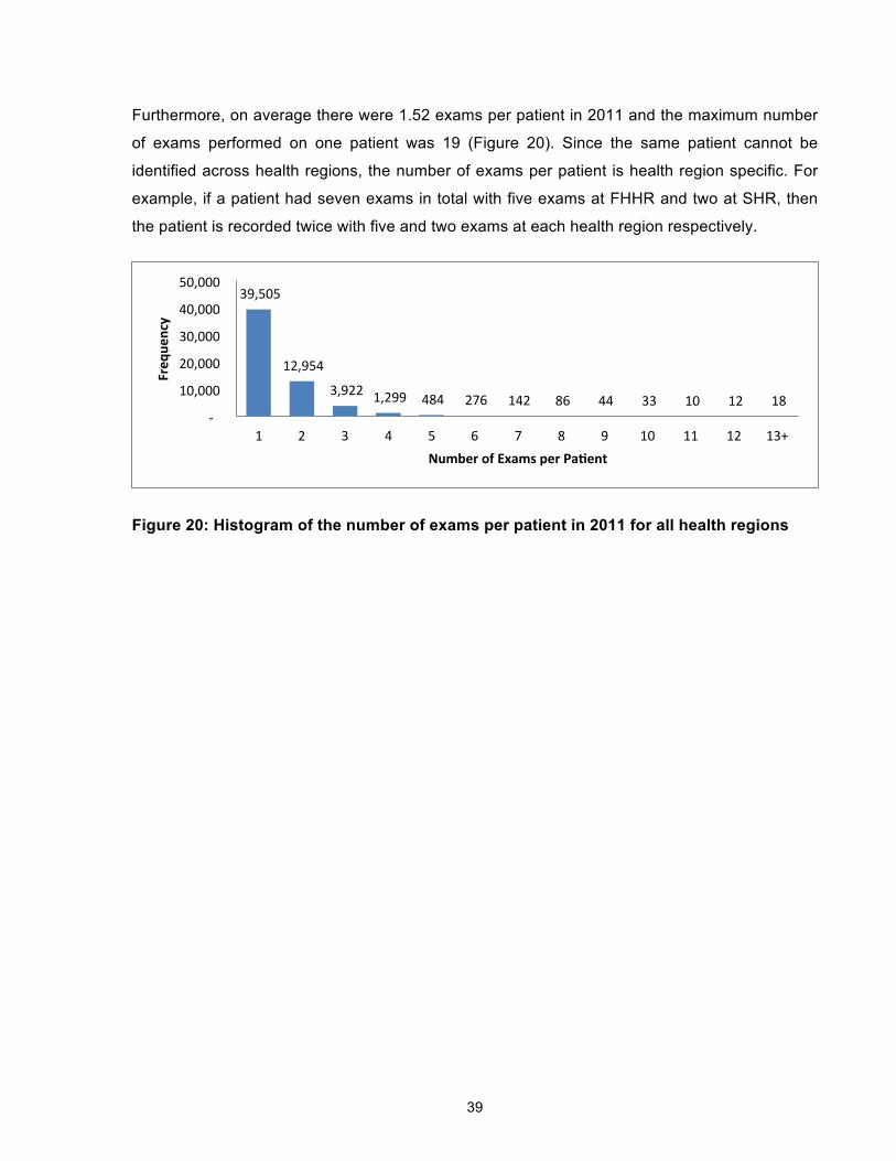
39

Furthermore, on average there were 1.52 exams per patient in 2011 and the maximum number

of exams performed on one patient was 19 (Figure 20). Since the same patient cannot be

identified across health regions, the number of exams per patient is health region specific. For

example, if a patient had seven exams in total with five exams at FHHR and two at SHR, then

the patient is recorded twice with five and two exams at each health region respectively.

Figure 20: Histogram of the number of exams per patient in 2011 for all health regions

 39,505    

 12,954    

 3,922      1,299      484      276      142      86      44      33      10      12      18      -­‐        

 10,000    

 20,000    

 30,000    

 40,000    

 50,000    

1   2   3   4   5   6   7   8   9   10   11   12   13+  

Freq

uency  

Number  of  Exams  per  Pa9ent  

40

4.5. Patient Access

Patient access was analyzed in terms of patient travel and wait times.

4.5.1. Patient Travel

Travel distances were estimated based on the patient’s postal code and CT facility. The

rectilinear distance was used to mimic driving on a street grid and calculations were made

based on each visit instead of number of exams. The mean travel distance for outpatients was

130.28 km whereas the median was 37.51 km (Table 7). The mean travel time for outpatients

was 52.7 minutes.

For urban CSDs, the median travel distance was 5.5km and for rural CSDs, the median travel

distance was 176.4km (Table 7). Similarly, rural and small CSDs had a much higher mean

travel time than medium and urban CSDs (Figure 21). Urban and rural CSD classifications were

determined by Statistics Canada [61].

Table 7: Provincial statistics for rectilinear travel distance (km) in 2011 by population

centre and rural area classification based on the patient’s residential postal code.

Population centre and rural area classification Mean Median 75th Percentile 95th Percentile

Rural Area 212.45 176.4 353.64 478.13

Small (1,000 – 29,999 pop.) 188.57 139.4 369.33 423.49

Medium (30,000 - 99,999 pop.) 24.23 3.71 5.9 180.81

Large Urban (100,000 or greater) 8.27 5.5 7.2 10.23

Overall Rectilinear Travel Distance (km) 130.28 37.51 183.65 447.43

41

Figure 21: Mean travel time to the health facility where CT exam was performed in 2011

from the patient’s residential postal code.

For outpatients from health regions without a CT facility, the majority did not go to the closest

CT facility. The outpatient’s health region of origin was based on their residential postal code.

Figure 22 shows that the majority of outpatients in health regions with a CT scanner went to the

CT facility in their health region. Saskatoon Health Region had the lowest proportion of

outpatients going out-of–region (2%). Prince Albert Parkland Health Region had the highest with

28.2% of outpatients going outside their health region for a CT exam in 2011. More research

needs to be done to understand why, but contributing factors include the teaching affiliations,

reputation, and physician referral patterns [62].

Overall, high percentages of outpatients from health regions without a CT facility went to Royal

University Hospital and to a lesser extent Saskatoon City Hospital and St. Paul’s Hospital with

the exception of outpatients from Sun Country RHA who are close to Pasqua Hospital in RQHR

(See Table 29 in Appendix E). Outpatients from Athabasca RHA went to Victoria Hospital

(63.3%) in Prince Albert Parkland Heath Region and Royal University Hospital (18.3%),

Saskatoon City Hospital (13.3%) and St. Paul’s Hospital (3.3%) in Saskatoon Health Region.

Mamawetan Churchill River Health Region and Kelsey Trial RHA have a similar pattern to

Athabasca. Outpatients from Keewatin Yatthé RHA primarily go to Lloydminster Hospital

(60.5%) in Prairie North RHA; Victoria Hospital (8.3%) in Prince Albert Parkland Health Region;

and Royal University Hospital (12.4%), Saskatoon City Hospital (13.6%) and St. Paul’s Hospital

(5.2%) in Saskatoon Health Region. Heartland RHA is surrounded by several health regions

with CT facilities and while outpatients go to all bordering health regions, 63% go to Saskatoon

Health Region.

112.0  

81.7  

33.6   35.4  

0  

20  

40  

60  

80  

100  

120  

Rural  Area   Small  (1,000  –  29,999  pop.)  

Medium  (30,000  -­‐  99,999  pop.)  

Large  Urban  (100,000  or  greater)  

Travel  Tim

e  (m

inutes)  

42

Figure 22: Proportion of outpatient visits from each health region that went to a CT

facility outside their health region and went to the closest CT scanner in 2011.

36.7%

11.9% 12.6%

84.1%

48.3% 51.8% 39.1%

21.7% 27.8%

4.9% 1.3%

42.3% 20.0%

63.3%

0.0% 0.4%

15.9%

51.7% 48.2% 60.9%

0.0% 0.4%

1.4% 0.7%

57.7%

0.0%

0% 10% 20% 30% 40% 50% 60% 70% 80% 90%

100%

Patient Health Region

Out-of-Region & Not Closest CT Out-of-Region & Closest CT

43

4.5.2. Wait Times

Patients have different target wait times depending on the urgency. Level 1 (Emergent) patients

have a target wait time of within 24 hours and are therefore not included in the wait time metrics.

In Table 8, LH and BUH in Prairie North RHA have the shortest wait times while CRH and

MJUH in FHHR have the highest wait times for non-urgent patients at 63 days and 48 days

respectively. All the estimated maximum wait times are within the targets. RQHR and SHR

report the wait times by 50th and 90th percentiles in Table 9. RQHR is not within targets for Level

2 and the 90th percentile for Level 3 patients exceeds the 30 day target. SHR also has longer

wait times for Level 2 patients in the 90th percentile.

Table 8: Estimated maximum wait time by number of days from day of referral to day of

appointment scheduling on December 31, 2011.

Facility Level 2 (Urgent) Level 3 (Semi-Urgent) Level 4 (Non-Urgent)

LH 0 0 7

MJU 1 7 48

BUH 2 2 7

VH 7 17 63

CRH 0 11 18

YRHC 4 15 40

Targeted Wait Time Within 7 days Within 30 days Within 90 days

Table 9: Wait time by number of days from referral to appointment scheduling on

December 31, 2011 for RQHR and Saskatoon Heath Region.

Locations Level 2 (Urgent)

Level 3 (Semi-Urgent)

Level 4 (Non-Urgent)

Regina Qu’Appelle 50% completed within (median) 9 22 24

90% completed within 28 36 46

Saskatoon 50% completed within (median) 5 8 15

90% completed within 9 17 19 Provincial Hospitals (RGH and RUH)

50% completed within (median) 6 14 23

90% completed within 21 30 45 Targeted Wait Time Within 7 days Within 30 days Within 90 days

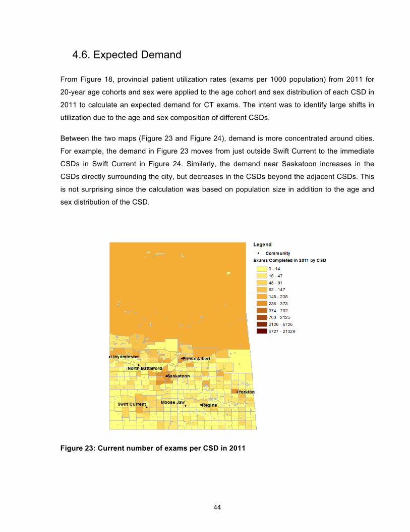
44

4.6. Expected Demand

From Figure 18, provincial patient utilization rates (exams per 1000 population) from 2011 for

20-year age cohorts and sex were applied to the age cohort and sex distribution of each CSD in

2011 to calculate an expected demand for CT exams. The intent was to identify large shifts in

utilization due to the age and sex composition of different CSDs.

Between the two maps (Figure 23 and Figure 24), demand is more concentrated around cities.

For example, the demand in Figure 23 moves from just outside Swift Current to the immediate

CSDs in Swift Current in Figure 24. Similarly, the demand near Saskatoon increases in the

CSDs directly surrounding the city, but decreases in the CSDs beyond the adjacent CSDs. This

is not surprising since the calculation was based on population size in addition to the age and

sex distribution of the CSD.

Figure 23: Current number of exams per CSD in 2011

45

Figure 24: Expected demand (number of exams) per CSD in 2011

46

4.7. Discussion

The results are discussed in comparison to other jurisdictions, how the different metrics relate to

each other, and the factors in projecting supply and utilization.

Comparing Saskatchewan to other jurisdictions

The provincial average operating hours per CT scanner are 58.64 hours per week. This is

slightly below the rest of Canada which operates for 60 hours per week on average [1].

However, in terms of CT provision by number of CT scanners per million population,

Saskatchewan is lower than Canada and the OECD average (Figure 25). From Figure 26, the

average CT scanner in Saskatchewan (6,777 exams/scanner) is performing slightly more

exams than the OECD average (6,312 exams/scanner) and far fewer than the Canadian

average (9,017 exams/scanner). The average CT scanner in Canada is performing 42.9% more

exams each year despite only running for 2.3% more operating hours than in Saskatchewan.

Given the variance in average exams per CT scanner (Figure 5) and exams per operating hour

(Figure 8) within Saskatchewan, this indicates that there is remaining capacity in the existing

system either through unused capacity or improving efficiency. In Figure 27, Saskatchewan also

has a patient utilization which is much lower than Canada’s and OECD average. This suggests

that although Saskatchewan’s existing system can perform more exams with similar operating

hours per year, there are also areas which are currently under-serviced. Variations in patient

utilizations have been found in Norway for CT exams by Lysdahl and Borretzen [25] due to

accessibility and socioeconomic factors. In 2002, patient utilization ranged from 56 exams per

1000 population in a rural area to 216 exams per 1000 population in Oslo, the largest city. The

average utilization was 108 exams per 1000 population.

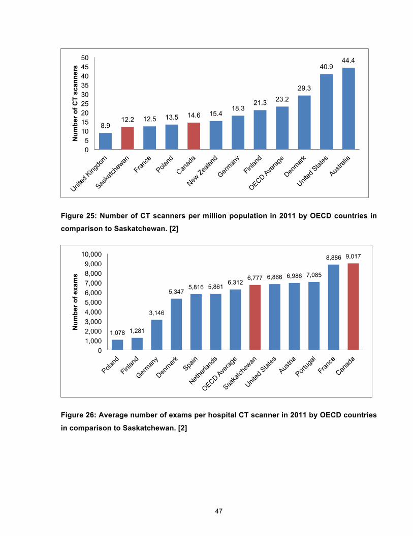
47

Figure 25: Number of CT scanners per million population in 2011 by OECD countries in

comparison to Saskatchewan. [2]

Figure 26: Average number of exams per hospital CT scanner in 2011 by OECD countries

in comparison to Saskatchewan. [2]

8.9 12.2 12.5 13.5 14.6 15.4

18.3 21.3 23.2

29.3

40.9 44.4

0 5

10 15 20 25 30 35 40 45 50

Num

ber o

f CT

scan

ners

1,078 1,281

3,146

5,347 5,816 5,861

6,312 6,777 6,866 6,986 7,085

8,886 9,017

0 1,000 2,000 3,000 4,000 5,000 6,000 7,000 8,000 9,000

10,000

Num

ber o

f exa

ms

48

Figure 27: Number of exams per 1000 population in 2011 by OECD countries in

comparison to Saskatchewan. [2]

CT utilization with patient utilization

In terms of exams per operating hour and proportions of patient types, there does not appear to

be a clear relationship when comparing Figure 7 and Figure 8. For example, even within the

same health region, Saskatoon City Hospital (SCH) and St. Paul’s Hospital (SPH) have similar

estimated exams per operating hour even though SCH has twice the percentage of outpatients

due to different patient populations. SPH has an exam rate of 319.8 exams per 1000 inpatients

in contrast to SCH that has only 43.8. SPH also has more emergency patients than SCH

(27.9% vs. 9.3%). From the literature, emergency departments have high CT exam rates such

as 705 and 394 scans per 1000 ED visits for patients 21 to 30 years old and 61 to 70 years old

respectively [63]. However, the emergency patient exam rate is 66.617 for SCH and 69.541 for

SPH. Furthermore, varying levels of patient complexity at different facilities may impact how

many exams can be done each hour.

29.1 37.3

70.8 83 90.4

104.1 128.2 129.3 130.1

172.1 178.5 180.3

256.8

0.0

50.0

100.0

150.0

200.0

250.0

300.0

Num

ber o

f exa

ms

per 1

000

pop.

49

CT utilization with patient access

BUH and YRHC have the same operating hours; they perform a similar number of exams per

year; and they have similar proportions of patient type and priority level. However, the wait times

at YRHC are much longer. A more detailed analysis of their processes and patients is needed to

understand the differences between the two facilities.

In terms of distance travelled by outpatients, 8 out of 13 health regions had 7% or more

outpatients go to Saskatoon Health Region which is expected because Royal University

Hospital is a tertiary hospital. Health regions with a CT facility also send patients to Saskatoon

City Hospital and St. Paul’s Hospital for outpatient CT exams. This may be due to referral

patterns or wait times in their facilities. For example, Victoria Hospital (PAPHR) has wait times

which are much longer than at neighbouring Battlefords Union Hospital and Prince Albert

Parkland Health Region has 17.9% of their patients going to SCH and SPH. More research

needs to be done in terms of why patients are being referred to specific institutions.

Projecting CT supply and utilization

From the metrics and discussion, it is clear that there are many factors that contribute to large

differences in exams performed at separate facilities beyond simply the number of operating

hours. Factors include, but are not limited to, the proportions of patient type, the patient

illnesses within each of those patient types, and referral practices [9].

For the expected demand calculation, only age and sex were used to adjust the utilization rates

for each CSD. However, the literature is clear that geographic factors impact patient utilization,

in particular, proximity to a CT scanner [25]. Furthermore, with the increase in the aging

population [60] and potential changes in migration and overall growth the demand may change

substantially. A more thorough analysis on socio-demographic and geographic factors,

including proportions of First Nations per CSD, should be done to improve demand projections.

50

Chapter 5. Capacity Planning Model for CT scanners

The previous chapter described the current situation with respect to CT supply, patient

utilization, and patient access. In this chapter, the metrics are used to inform the parameters of

the model and provide context to the results. This chapter begins with a description of the

problem specific to CT scanner capacity planning and then describes the model assumptions

and formulation. Calculations for the model’s input data are discussed followed by descriptions

of the model scenarios. Scenarios results are presented to understand cost and access trade-

offs and the sensitivity of the results.

5.1. The Problem

The goal of the proposed model is to determine for a specified planning horizon: 1) where CT

scanners should be located, and for each location, 2) how many CT scanners are needed,

3) how many operating hours are necessary, and 4) when capacity changes are needed while

achieving targets for covering demand within facility catchment areas and minimizing cost. The

size of the catchment area is determined by the maximum patient travel time.

In the model we assume that a proportion of demand from each location (e.g., community,

census subdivision) will be assigned to a facility if the demand is within the facility’s catchment

area and capacity is available at the facility. The minimum coverage percentage determines the

amount of assigned demand. However, all demand must be met. In the case that demand is not

assigned to a specific facility, then the unassigned demand has no patient travel time restriction.

It is assumed that any facility can fulfill unassigned demand which leads to longer travel times

for the remaining percent of demand. Any unused capacity at existing facilities can be used to

meet the unassigned demand. If there is insufficient capacity, then more capacity needs to be

added to the system through adding capacity to the existing facilities or opening a new facility.

The set of potential CT facilities is predetermined to ensure suitability.

To identify overtime utilization and leftover capacity, a week is segmented into smaller units

based on shift work. Each segment is called a shift and is considered part of regular time. We

made the simplifying assumption that a shift is 40 hours. The sum of shifts for each facility

constitute the total number of regular operating hours per week and the model does not

determine how the hours are spread during the week. There are two ways to add capacity to

existing facilities: staff another shift and add a new CT scanner. An open facility can have

multiple CT scanners, which each need to be staffed for at least one shift and can be operated

51

for a specified maximum number of shifts (e.g. 3 shifts for a total of 24 hours per day). When

there are multiple shifts at the same facility, the assumption is that shifts are running in series on

the same CT scanner. If there is more than one CT scanner at a facility, then shifts can run in

parallel. There is no limit on the number of CT scanners a facility can hold. When demand

assigned to a facility exceeds the capacity of a shift, then it will be charged at an overtime rate.

When the cost of overtime exams exceeds the cost of a shift, then another shift is added to the

facility to increase the regular operating hours. Shifts are removed from a facility at a dummy

cost called a shift removal cost. Another CT scanner is added to the facility in two situations: 1)

when the number of shifts required exceeds the maximum number of shifts and the cost of

overtime exams is more than the cost of both a CT scanner and one shift or 2) the assigned

demand exceeds the maximum capacity of the CT scanners.

In order to build a new CT facility, the catchment area of existing facilities must need the new

CT facility to reach the minimum percentage of covered demand. To reach more demand within

the maximum travel time, another CT facility is built at the cost of opening and purchasing a CT

scanner. To ensure a balance between cost and access, many health care systems will have

existing CT scanners which should be incorporated into the capacity plan. Therefore, the

opening cost is only incurred when there is no pre-existing facility.

5.2. Model Development

To develop the model formulation, the following assumptions are made:

Assumption 1: A minimum percentage of patient demand must be able to reach a CT scanner

within specified travel time radius.

Assumption 1 may not hold because of possible referral patterns, central appointment booking,

and patient activity spaces may bring patients outside of the specified travel radius [20]. If

central appointment booking were implemented, it may give patients earlier appointments at the

expense of longer travel times. Patients may also prefer different locations depending on where

their other life activities occur [20]. However, this assumption matches rural access standards

for healthcare services set by British Columbia [64] and Ontario [65].

52

Assumption 2: New CT scanners could be placed at a specific set of candidate locations.

Assumption 2 acknowledges that there are many factors which contribute to a CT facility

candidate such as existing hospitals, human resources and road infrastructure.

Assumption 3: CT scanners cannot be relocated or closed.

Assumptions 3 may not hold when CT scanners get old and need to be replaced. In addition to

a large capital investment, CT scanners require substantial human resources and are in high

demand for diagnostics, especially for emergency and inpatients. While it may be possible for a

CT scanner to be relocated, it is unlikely.

Assumption 4a: The maximum number of exams a CT scanner can complete each year will

remain constant in each time period in the planning horizon.

Assumption 4b: The duration of CT exams does not change.

Assumptions 4a and 4b imply that there will not be improvements which make CT scanners

more efficient. Over a 20-year planning horizon it is possible for new technology to be invented

that dramatically impacts utilization rates by allowing more CT scans to be done each day.

However, when technology improves, more images tend to be ordered per exam [66]. This

suggests that exam duration may not change substantially. Furthermore, although different

types of exams take various lengths of time, the aggregate exam time in a year may vary less

than specific exam types.

Assumption 6: Costs do not differ depending on the geographic location or facility type.

Costs associated with CT scanners will not change (exams, supplies, technologists) depending

on where CT exams are provided. This may not hold due to transportation costs and incentives

to practice in less popular locations.

Assumption 7: The real cost of goods and services does not change.

As the cost of goods and services will increase with inflation, the real cost to the system does

not change. Furthermore, the increase in cost of a CT scanner and facility due to inflation is

negligible compared to the overall cost of the CT scanner system.

53

Assumption 8: One CT scanner at each candidate location can be added in each time period.

This assumption may hold when the demand within a candidate location’s catchment area does

not increase dramatically. For example, if the unused overtime capacity for a CT scanner is

18,837 exams and the demand rate is 83 exams per 1000 population, then the population would

need to increase by more than 226,952 people to require a second CT scanner in the same

time period at the same facility. This assumption was made to improve the solvability of the

model. If more than one CT scanner can be added to each candidate location in each time

period, this will add complexity to the model.

Assumption 9: It costs less to add a new CT scanner at an existing facility than open a new

facility with a new CT scanner.

According to the CIHI report [1], in general it was less expensive to add CT scanners to existing

facilities than to build a new CT facility. However, the costs of renovating the rooms and

buildings for CT scanners are in the range of $400K to $1.8M. There may be certain

circumstances where this assumption does not hold.

Assumption 10: All CT scanners can do all types of scans.

Different CT scanners are capable of different types of CT images. For example, a volumetric

computed tomography scanner allows for 3D imaging, but this type of CT scanner is only

available at tertiary hospitals. However, the majority of scans can be completed on just 16-slice

CT scanners [67] and this assumption simplifies the model for most scans.

Assumption 11: Costs during regular operating hours are the same regardless of the number

of exams completed.

The current formulation assumes that the cost of a shift is the same regardless of how much

unused operating capacity is left. According to Saskatoon Health Region’s budget from April

2011 to March 2013, operating and personnel costs comprise of 92.2% of expenses. The

material costs of exams only make up the remaining 7.8%. While this assumption overestimates

the cost of a shift if there is idle time, the additional cost is a small percentage of the overall

costs because of the operating and personnel costs.

54

5.2.1. Formulation

Description: Suppose there is a set of I CT demand locations and a set of J CT facility

locations to be planned for in T time periods. CT demand changes magnitude with time t for

each demand location i. A proportion of demand at location i is covered by an open CT facility in

location j in time t. The province must have the capacity to meet all the demand regardless of

CT catchment areas. When a new CT facility is built, it incurs an opening cost. Additional CT

scanners can be added to the existing CT facilities. Shifts can be added to each CT scanner in

order to increase the normal operating capacity in each time period. Furthermore, when a CT

scanner is assigned more exams than the normal operating capacity, it incurs an overtime

surcharge to the cost per additional exam.

Indices:

i = 1... I: Index of CT demand locations

j = 1... J: Index of CT facility locations

t = 0…T: Index of capacity planning time periods

Parameters:

Demandit = number of CT exams that need to be performed in area i at time t

DemandTotalt = Demand!"!!!!

MinCoverage = minimum percentage of total demand that must be covered with a maximum

patient travel time

aij = { 1 if CT demand in area i is within a maximum patient travel time of location j, 0 otherwise}

CapMax = maximum number of exams for each CT scanner

CapShift = maximum number of exams in a shift

MaxShifts = maximum number of shifts per CT scanner which make up regular operating hours

CostOpen = cost of opening a new CT facility

CostCT = cost of adding a CT scanner to an open facility

55

The cost of opening a new CT facility is separate from the cost of purchasing a CT

scanner. Therefore, to open a new CT facility, the total cost is the cost of opening the

facility plus the cost of the new CT scanner (Total Cost of New CT Facility = Cost Open

+ CostCT).

ExamCost = cost for each exam completed during regular operating hours

OvertimeSurcharge = percent increase in cost per exam that exceeds a CT scanner’s normal

operating capacity

ShiftRemovalCost = cost of removing a shift from a CT facility

To initialize the model: CTTotalj0 = number of current CTs at location j at time 0

Decision Variables:

xijt = fraction of demand covered at location i by a CT at location j at time t

yjt = {1 if a new CT is placed in location j at time t, 0 otherwise}

CTTotaljt = total number of CTs at location j at time t = CTTotal!"!! +  y!"

zj = {1 if a new facility is placed at location j in any period, 0 otherwise}

z! ≥ y!" − CTTotal!"    ∀  j  ∀  t

CToverjt = number of assigned exams exceeding normal operating capacity at location j at time t

CTunderjt= number of exams below the normal operating capacity at location j at time t

Shiftsjt = number of sets of regular operating hours at location j at time t

UnassignedDemandt = number of unassigned exams at time t

UnassignedOverjt = number of unassigned exams completed in overtime at location j at time t

UnassignedUnderjt = unused regular operating capacity at location j at time t (measured in

number of exams)

ShiftRemovedjt = number of shifts removed from a location j at time t

56

ShiftAddedjt = number of shifts added to a location j at time t

Model:

The following is a formulation for the dynamic CT scanner facility location problem.

Minimize    CostOpen z! +  CostCT  y!"!!!!

!!!!  !

!!! +  

OvertimeSurcharge*ExamCost    CTover!"!!!!

!!!! +   UnassignedOver!!

!!!  +  

ExamCost*CapShift  Shifts!"!!!!

!!!!  +  ShiftRemovalCost    ShiftRemoved!"

!!!!

!!!!  

s.t.  

x!"#Demand!"!!  ≥ MinCoverage ∗ DemandTotal!  ∀  t         (1)    

Capmax   CTTotal!"! ≥ DemandTotal!  ∀  t             (2)  

x!"#Demand!"! = CapShift   ∗ Shifts!" + CTover!" − CTunder!"    ∀  j,∀t       (3)  

CTover!" ≤ CapMax ∗ CTTotal!"  −  CapShift ∗ Shifts!"    ∀  j,∀t         (4)    

 x!"# ≤ a!"CTTotal!"  ∀  i  ∀  j  ∀  t                 (5)  

x!"#! ≤ 1  ∀  i  ∀  t                   (6)  

z! ≥ y!" − CTTotal!"    ∀  j  ∀  t                   (7)  

CTTotal!" = CTTotal!"!! +  y!"    ∀  j  ∀  t   ≥ 1             (8)  

Shifts!" ≤ MaxShifts ∗  CTTotal!"  ∀  j  ∀  t               (9)  

Shifts!" ≥  CTTotal!"  ∀  j  ∀  t                 (10)  

Shifts!"!! −  Shifts!" =  ShiftRemoved!" −  ShiftAdded!"∀  j  ∀  t         (11)  

DemandTotal! − x!"#Demand!"!! = UnassignedDemand!  ∀  t       (12)  

UnassignedDemand! − CTunder!"! = UnassignedOver! − UnassignedUnder!  ∀  t   (13)  

57

y!"  binary  ∀  j  ∀  t                   (14)  

z!  binary  ∀  j                     (15)  

CTTotal!" ≥ 0     ∀  j  ∀  t                   (16)  

CTover!" ≥ 0     ∀  j  ∀  t                   (17)  

CTunder!" ≥ 0    ∀  j  ∀  t                   (18)  

Shifts!" ≥ 0  integer    ∀  j  ∀  t                 (19)  

UnassignedDemand! ≥ 0      ∀  t                 (20)  

UnassignedOver! ≥ 0   ∀  t                 (21)  

UnassignedUnder! ≥ 0      ∀  t                 (22)  

ShiftRemoved!" ≥ 0    ∀  j  ∀  t                 (23)  

ShiftAdded!" ≥ 0    ∀  j  ∀  t                 (24)  

0   ≤ x!"# ≤ 1    ∀  i  ∀  j  ∀  t                   (25)  

The objective is to minimize the cost of opening new CT facilities, adding new CT scanners,

overtime exams, regular operating hours, and shift removal. The exam cost is multiplied by the

capacity during regular operating hours to account for salaries, operating costs, and materials.

The overtime surcharge incorporates the additional variable costs such as overtime wages paid

to staff.

Constraint (1) ensures that a minimum percentage of the total provincial demand is covered in

each time period. For example, if the minimum coverage is 95% and the maximum travel time is

30 minutes, then a minimum of 95% of demand can reach a CT scanner in 30 minutes.

Constraint (2) ensures that there is enough existing capacity, using the maximum CT capacity,

from all the implemented CT scanners to meet all of the provincial demand each time period.

58

Constraint (3) calculates the assigned demand, the number of shifts required to cover both

assigned and unassigned demand, and the resulting overtime exams and unused exam

capacity for each CT facility in each time period.

Constraint (4) checks that the overtime is within the overtime capacity for each CT facility in

each time period.

Constraint (5) makes sure that the assigned demand to the CT facility is within the maximum

travel time of the CT facility based on the feasibility matrix, aij.

Constraint (6) prevents covered demand from being assigned more than once.

Constraint (7) opens a new CT facility when the initial CT scanner needs to be built and ensures

the opening cost is only incurred for new CT facilities.

Since CT scanners can only be added, Constraint (8) does not allow CT facilities to be closed

and updates the total number of CT scanners at each candidate location in each time period.

For Constraint (9), the number of shifts at each location and time period cannot exceed the

maximum number of shifts allowed for each CT scanner.

Constraint (10) ensures that each CT scanner is run for at least one shift.

Constraint (11) calculates the number of shifts which are added and removed for each CT

facility for each time period.

The amount of unassigned demand in each time period is calculated in Constraint (12).

Constraint (13) calculates the number of unassigned overtime exams and unused exam

capacity in the system for each time period.

z!  and  y!" are binary decision variables in Constraint (14) and (15) respectively. Since  y!" is

binary, it assumes that there will be no more than one CT scanner added each year. For z!,  a

facility is either opened or not and for y!", a CT scanner is added to an open facility or not. In

Constraint (16), CTTotal!" is a real number, but only increments by 1 because y!" is binary.

CToverjt, CTunderjt, UnassignedDemandt, UnassignedOvert, UnassignedUndert, ShiftRemovedjt,

and ShiftAddedjt are positive real numbers. Shiftsjt is integer and non-negative since each CT

scanner can have multiple shifts and there cannot be partial shifts. x!"# is the fraction of demand

59

covered by a CT so its values are continuous from 0 to 1. While partial CT exams are not

realistic, having fractional exams does not have a large impact on the model results and

improves computation time.

5.3. Model Inputs for Saskatchewan’s CT Capacity Plan

The capacity planning model will output the number of required CT scanners, the locations they

are placed, the year they should be implemented, and the utilization level in each year. A long

planning horizon of 19 years (until 2030) was based on results from population projections of

Saskatchewan from Statistics Canada. However, population projections and CT scanner

technology will change over time. This will alter demand patterns and capacity levels, which

could have a substantial impact on accuracy of the capacity plan. The model should be re-run

with new information as necessary to create an updated capacity plan. This section explains

the model input data calculations and resulting input data for applying the model to

Saskatchewan.

5.3.1. Input Data Calculations

All the model parameters were calculated from various sources for the model.

Existing CT Facilities

The decision variable, CTTotaljt, was initialized based on the current CT scanner locations in the

province (See Table 6). Data on existing CT facilities were collected from each of the CT-

equipped health regions. The assumption for most of the scenarios is that policy makers would

want to build upon existing resources to reduce costs. It also acknowledges that there are many

reasons why a CT facility is chosen beyond the demand within a certain catchment area. In this

model, existing CT facilities can install additional CT scanners. Therefore, only the cost of the

new CT scanner is incurred for existing CT facilities and not the cost of building a new CT

facility.

Candidate Facility Locations

Potential new CT facilities were the existing hospitals in Saskatchewan due to the impact on

improving care by providing the ability to diagnose inpatients and emergency patients on

premise. Freestanding clinics could be considered for outpatients only; however, they tend to be

more efficient for areas with a high population density and our research focuses on improving

60

access for remote and rural populations [1]. For the purposes of this model, only existing

hospitals were considered candidate facility locations.

Hospitals are given a facility designation based on the types of services they provide according

to The Facility Designation Regulations [68]. Currently, all provincial and regional hospitals have

CT scanners. All district hospitals were chosen as potential CT facilities because they were the

next largest hospital classification. District hospitals are larger than community hospitals, so

from a policy perspective, district hospitals would require less investment in infrastructure to

implement CT scanners than community hospitals. Northern hospitals are a type of community

hospital which is more focused on servicing northern Saskatchewan populations. Due to our

interest in patient access, all three northern hospitals (i.e. La Loche Health Centre, La Ronge

Health Centre, and St. Joseph's Health Centre) were included so there would be potential CT

facilities north of existing facilities.

In summary, hospitals classified as provincial, regional, district, and northern were included in

this model as candidate facility locations.

Patient Travel Time Calculations

As described in the Methods Section 0, travel times between the census subdivision centroid

and all candidate facility locations were estimated in ArcGIS using the road network and

rectilinear travel distances. The maximum travel times form the catchment area of the CT

facilities. A study has shown that as travel burden increases (time increases), patient utilization

and access to mental health services will decrease [19]. For CT specifically, geographic location

may explain lower scanner utilization in a region [1].

The travel times between each census subdivision and CT facility are combined with the

maximum travel time to create the binary aij parameter.

Cost of opening a CT facility

Estimates of the cost to renovate a facility for its first CT scanner was based on previous

implementations across Canada, which separated the renovation cost from CT scanner costs.

Data were obtained from the CIHI report [1] and press releases from the Saskatchewan Ministry

of Health [69 - 73]. Renovation costs ranged substantially from $400K to $1.8M.

The average renovation cost was $1.25M, which is used in the capacity planning model.

61

Cost of a CT scanner

For the estimate on the cost of a single CT scanner, the CIHI report [1] used the value $1.7M

per CT scanner which was based on the average cost of CT scanners in Ontario. This value

was checked against the Emergency Care Research Institute 2012 white paper [74] on CT

scanners which included the average vendor-quoted cost for a CT scanner in addition to the

service cost which was $1.67M for “premium” scanners. Hence, the cost of an additional CT

scanner in the capacity planning model was $1.7M.

Exam cost and overtime surcharge of additional exams

The exam cost and overtime surcharge of additional exams was calculated based on the

average exam cost in Saskatoon Health Region excluding physician remuneration and benefits

in 2011. Each exam costs $62.26 for the technologist, operations cost, and materials. This cost

does not separate the operating costs during regular operating hours from overtime hours since

our cost data does not distinguish between the two times of operation. Therefore, when the

cost of a shift is calculated in the model, it slightly overestimates the cost of a shift if there is

unused exam capacity during regular operating hours.

The overtime surcharge is estimated to be 50% more than the exam cost of a regular exam to

reflect the typical time and a half paid for overtime.

CT scanner capacity

The average number of exams per hour is used to estimate CT scanner capacity. We had

obtained the time the exam began from Moose Jaw Union Hospital, Victoria Hospital,

Battlefords Union Hospital, Lloydminster Hospital and Yorkton Regional Health Centre. This

filters for exams completed within regular operating hours and the average number of exams

per hour was 2.26. The other facilities did not have exam times. Their estimated exams per hour

is 2.61 which is higher due to the inclusion of overtime exams. For calculating the capacity

parameters, 2.26 was used as the average number of exams per hour.

The smaller CT facilities in Saskatchewan run for eight hours a day and five days a week, thus a

shift is defined as 40 hours per week. Hence, the annual CT capacity was 4,700 exams for the

purpose of a regular shift and the maximum annual CT scanner capacity is 19,743 exams per

year based on operating a CT scanner 24 hours a day and 52 weeks a year without holidays.

62

Demand calculations

Demand from 2012 to 2030 for each CSD is estimated using provincial patient utilization rates

based on 20-year age cohorts and sex, provincial population estimates from 2011 to 2014, and

M1 provincial growth rates from 2014 to 2030. 20-year age cohorts were chosen to achieve a

larger sample size and thus more accurate utilization rates. The M1 scenario has a medium

growth rate and historical migration trends. Population projections for each demand area i were

multiplied by 2011’s average utilization rates by sex and age cohort. The yearly provincial

growth rates by age cohort and sex were applied to each census subdivision (Appendix B).

There was no adjustment made for different exam procedure groups and patient types

(emergency, inpatient, outpatient). See Methods Section 3.1.4 and 0 for more details on the

population projection calculations.

As a result, the demand calculations assume that the demand rate will remain constant;

provincial growth by age cohort and sex is the same across all census subdivisions; and

demand rate is independent of proximity to a CT scanner.

The assumption that the demand rate will remain constant in each time period and each

demand location over the planning horizon may not hold since new technology can change

usage patterns by increasing the range of possible diagnosis thereby increasing the need for CT

scans. Furthermore, studies in mental health [19] and radiological services [25] have shown that

areas with less access to medical equipment have lower utilization rates making it unlikely that

the utilization rate in Saskatchewan is independent of proximity to a CT scanner. If there is less

access to care, then low utilization rates are more reflective of low access and may still have a

higher demand rate than the utilization rate suggests.

Maximum Shifts

Given the current operating hours for CT scanners in Saskatchewan (Table 6), each shift is the

equivalent of 40 hours a week with a maximum of 3 shifts each year. While it is possible to run a

4th shift for the remaining hours in the week, none of the existing CT scanners has regular

operating hours 24 hours a day.

63

Shift Removal Cost

This is a dummy cost to prevent the model from moving shifts back and forth between different

facilities. A shift cost of $100K was used with no impact on the objective function (See Section

5.6.4).

5.3.2. Resulting Input Data

Based on the calculations and sources in Section 5.3.1 (Input Data Calculations), the values in

this section were used as parameters in the model unless otherwise noted in the scenario.

For the indices, the set of I demand locations is 959 since each CSD is considered a CT

demand location. All CSDs in Saskatchewan are used for completeness. The set of J candidate

facility locations includes all 23 existing and potential CT facility locations (See Table 31 in

Appendix F). There are 19 time periods T, so that the model runs from 2012 until 2030. The

feasibility matrix, aij,, is adjusted based on the maximum travel time.

The base case parameter values are:

CapMax = 19, 743 exams per year per CT scanner

CapShift = 4,700 exams per year per shift

CTTotalj0 = See Table 6

CostOpen = $1.7M

CostCT = $1.25M

ExamCost = $62.26 per exam

OvertimeSurcharge = 50% extra

MaxShifts = 3 per CT per year

ShiftRemovalCost = $100K

64

5.4. Solution Approach

As described in Methods Section 0, in order to obtain results, AMPL model files (.mod) and data

files (.dat) were created using MATLAB v.7.12.0.635 (R2011a). In AMPL v.20140331, the

CPLEX solver was called to obtain results. The run time was limited to 1 hour.

Limiting the run time to an hour means that the optimal solution was not necessarily found. To

check whether limiting the run time to an hour would result in substantially different results, the

model was run for 2 hours, 30 minutes, 15 minutes, and 10 minutes with a 2-hour travel time

and 90% minimum coverage. The results for all run times were the same except for the run time

of 10 minutes. With a 10 minute run time, the model finds a worse solution. However, run times

of 15 minutes and 2 hours output the same results. Furthermore, the model is trying to find an

optimal solution to a problem where all the model parameters have been estimated. Since a

model’s result is only as accurate as the input data, having an optimal solution is not crucial.

The relative mixed-integer program (MIP) gap is the percent difference between a theoretical

optimal answer from a linear program relaxation and the current best answer. So a difference of

1% suggests that the solution is within 1% of the theoretical optimal answer. If the relative MIP

gap is too high, then it implies that the solution may not be optimal.

5.5. Scenarios and Sensitivity Analysis

The model was used to run several scenarios to analyze the results based on various

parameters. The feasibility of access and cost was assessed analytically. The three main model

scenarios were:

Scenario 1: Trade-off between access and cost

Scenario 2: Covering provincial demand

Scenario 3: Green field

Furthermore, a sensitivity analysis was conducted to understand how the model results would

change if key parameters were modified.

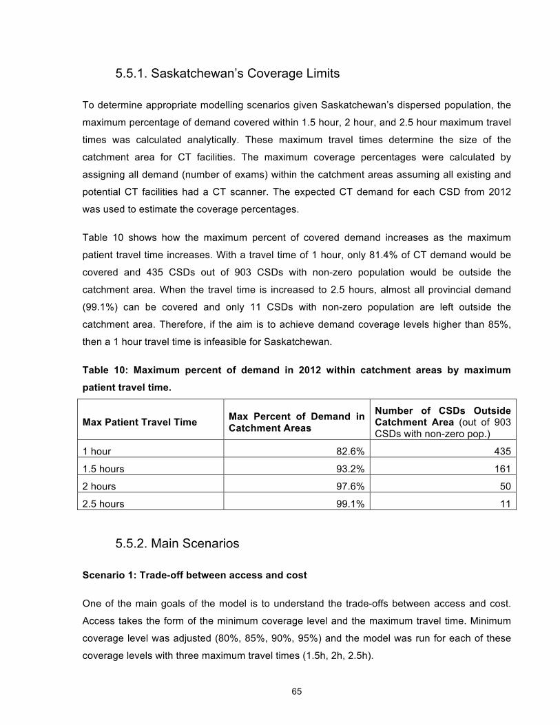
65

5.5.1. Saskatchewan’s Coverage Limits

To determine appropriate modelling scenarios given Saskatchewan’s dispersed population, the

maximum percentage of demand covered within 1.5 hour, 2 hour, and 2.5 hour maximum travel

times was calculated analytically. These maximum travel times determine the size of the

catchment area for CT facilities. The maximum coverage percentages were calculated by

assigning all demand (number of exams) within the catchment areas assuming all existing and

potential CT facilities had a CT scanner. The expected CT demand for each CSD from 2012

was used to estimate the coverage percentages.

Table 10 shows how the maximum percent of covered demand increases as the maximum

patient travel time increases. With a travel time of 1 hour, only 81.4% of CT demand would be

covered and 435 CSDs out of 903 CSDs with non-zero population would be outside the

catchment area. When the travel time is increased to 2.5 hours, almost all provincial demand

(99.1%) can be covered and only 11 CSDs with non-zero population are left outside the

catchment area. Therefore, if the aim is to achieve demand coverage levels higher than 85%,

then a 1 hour travel time is infeasible for Saskatchewan.

Table 10: Maximum percent of demand in 2012 within catchment areas by maximum

patient travel time.

Max Patient Travel Time Max Percent of Demand in Catchment Areas

Number of CSDs Outside Catchment Area (out of 903 CSDs with non-zero pop.)

1 hour 82.6% 435

1.5 hours 93.2% 161

2 hours 97.6% 50

2.5 hours 99.1% 11

5.5.2. Main Scenarios

Scenario 1: Trade-off between access and cost

One of the main goals of the model is to understand the trade-offs between access and cost.

Access takes the form of the minimum coverage level and the maximum travel time. Minimum

coverage level was adjusted (80%, 85%, 90%, 95%) and the model was run for each of these

coverage levels with three maximum travel times (1.5h, 2h, 2.5h).

66

Adjusting travel time and minimum coverage level will lead to differences in the total cost which

can be presented to the decision maker, who can determine which parameter assumptions and

costs are most appropriate. By adjusting coverage percentage, the relative financial impact of

increasing the percentage of the population that are within the maximum travel distance can be

assessed. The maximum travel time defines the travel burden for patients and needs to be

understood relative to the financial impact on the province. This scenario also assumes that the

province will build upon its existing CT facilities.

Scenario 2: Covering provincial demand

To get a better understanding of the capacity and costs if travel time was not a limiting factor,

scenario 2 was run with the minimum coverage level set at 100% and the maximum travel time

20.2 hours since it was the highest travel time for CSDs with demand to a CT facility.

Selecting a base scenario

For sensitivity analysis and green field scenario, the base case was for a minimum coverage

level of 90% and the maximum travel time of 2 hours. From the metrics, the 75th percentile of

patients travelled 183.65 km which would take approximately 2 hours to drive. For basic

inpatient services, guidelines on rural health service provision from British Columbia [64] and

Ontario [65] indicate a maximum travel time of 2 hours at a 95% coverage level and 1 hour at a

90% coverage level, respectively. The next health provision category is tertiary level care with a

maximum travel time of 4 hours for both British Columbia and Ontario. Furthermore, a national

study was conducted on travel time to hospitals for women giving birth [75] and it uses 2 hours

as the travel time threshold, which further suggests that travelling 2 hours is the maximum

appropriate travel time. For the coverage level, there is at least 90% coverage in British

Columbia and Ontario. Given the results in Section 5.5.1, a 95% coverage level may not be

practical for Saskatchewan.

Scenario 3: Green Field

In scenarios 1 and 2, it is assumed that current resources will continue to be open, which

reduces capital costs in the model. In scenario 3, this assumption is removed by starting with no

CT scanners. Using these results, a comparison between the current situation and an

alternative set of facilities can be made. Although this scenario may not be realistic given

emergency care situations and the benefits to hospital inpatients, it provides insight into the

minimum viable facilities needed to meet the access requirements.

67

5.5.3. Sensitivity Analysis

These parameter ranges are based on research from Section 5.3.1 and were verified by a

radiologist. Key parameters are the cost of opening a new facility, cost of a CT scanner, cost of

an exam, overtime surcharge percentage, and number of exams in a shift.

For the cost of a new CT facility, there is a large range of values because each hospital needs

different renovations to support a CT scanner. From the CIHI report [1]and press releases from

the Saskatchewan Ministry of Health [69 - 73], renovation costs ranged from $0.400M to $1.8M.

$0.625M was also run since it is half the value used in the model.

CT scanner costs depend on which scanner is purchased (e.g., 16-slice or 64-slice). From the

CIHI report [1]and press releases from the Saskatchewan Ministry of Health [69 - 73],costs

ranged from $0.850M to $2M. However, the most likely cost range is $1M to $1.5M per CT

scanner.

Exam costs were estimated based on Saskatoon Health Region’s operating budget. However,

each facility will have different exams costs due to efficiency, human resources, and other

factors. Therefore, sensitivity analysis was run on costs from $50 to $90 at $20 intervals.

The overtime surcharge was originally based on human resources costing time and a half.

However, this may not be the case and there may be additional factors contributing to the cost

of a CT exam. Overtime surcharge was set to 100% extra, which doubles the cost of an exam.

Annual shift capacity is a key parameter since it impacts the operating costs and resulting

number of overtime exams and unused exam capacity. To adjust the annual shift capacity, a

sensitivity analysis based on changing the exam rate four times. If the exam rate increased by

10% (2.49 exams per hour), a total of 5179 exams would be completed in one shift. The

estimated exams per operating hour in the province was an average of 2.61 exams in 2011.

Assuming the same number of operating hours a year, the annual shift capacity is 5428. CIHI

[1] reported a different number of exams per operating hour by CT type. The average was 3.1

for 64-slice, 16-slice, and 8-slice CTs combined which resulted in a shift capacity of 6448

exams. SPH had the highest utilization in the province with 3.93 exams per hour in 2011 and an

annual shift capacity of 8174 was used.

A high shift removal cost of $100K was used, so a scenario with a low cost of $20 was run to

show whether this effected how many shifts were removed.

68

High and low demand scenarios were run based on Statistics Canada’s population projections

and their assumptions for Scenario H and L respectively. The increased assumptions for

Scenario H’s high growth are a total fertility rate of 1.9 births per woman and a life expectancy of

85.4 years for males and 88.4 years for females by 2036. Immigration has a constant national

effective of 265,000 immigrants for the first three years and then a constant national immigration

rate of 0.9%. The decreased assumptions for Scenario L’s low growth are a total fertility rate of

1.5 births per woman and a life expectancy of 82.3 years for males and 86.0 years for females

by 2036. Immigration has a constant national effective of 240,000 immigrants for the first three

years and then a constant national immigration rate of 0.9%.

Using the base scenario, the model was run for each of the following values:

! Cost of a new CT facility (CostOpen) = $0.4M, $0.625M, $1.8M

! Cost of a CT scanner (CostCT) = $0.850M, $1M, $1.5M, $2M

! Exam Cost = $50, $70, $90

! Overtime surcharge on exam cost (OvertimeSurcharge) = 100%

! Exams per operating hour (Shift Capacity) =2.49 (5179 exams), 2.61 (5428 exams), 3.1

(6448 exams), 3.93 exams per hour (8174 exams)

! Shift Cost = $20

! Demand = high, low

This sensitivity analysis allows a better understanding of how substantial changes in parameters

could impact the results of the model. This is particularly important since all the parameters are

based on estimates.

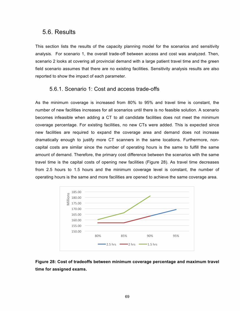
69

5.6. Results

This section lists the results of the capacity planning model for the scenarios and sensitivity

analysis. For scenario 1, the overall trade-off between access and cost was analyzed. Then,

scenario 2 looks at covering all provincial demand with a large patient travel time and the green

field scenario assumes that there are no existing facilities. Sensitivity analysis results are also

reported to show the impact of each parameter.

5.6.1. Scenario 1: Cost and access trade-offs

As the minimum coverage is increased from 80% to 95% and travel time is constant, the

number of new facilities increases for all scenarios until there is no feasible solution. A scenario

becomes infeasible when adding a CT to all candidate facilities does not meet the minimum

coverage percentage. For existing facilities, no new CTs were added. This is expected since

new facilities are required to expand the coverage area and demand does not increase

dramatically enough to justify more CT scanners in the same locations. Furthermore, non-

capital costs are similar since the number of operating hours is the same to fulfill the same

amount of demand. Therefore, the primary cost difference between the scenarios with the same

travel time is the capital costs of opening new facilities (Figure 28). As travel time decreases

from 2.5 hours to 1.5 hours and the minimum coverage level is constant, the number of

operating hours is the same and more facilities are opened to achieve the same coverage area.

Figure 28: Cost of tradeoffs between minimum coverage percentage and maximum travel

time for assigned exams.

150.00  

155.00  

160.00  

165.00  

170.00  

175.00  

180.00  

185.00  

80%   85%   90%   95%  

Millions  

2.5  hrs   2  hrs   1.5  hrs  

70

Table 11 summaries the new facilities opened for each scenario. With a travel time of 2.5 hours,

no facilities were added until minimum coverage reached 95%. At 95%, four new facilities were

opened. This coverage level was infeasible with a 2 hour and 1.5 hour travel time. With a 2 hour

travel time, no facilities were opened until there was a 90% coverage level, where two new

facilities were opened. These two scenarios increase operating hours in the same years, but

distribute the hours differently between the facilities as shown in Figure 29 and Figure 30. A

travel time of 1.5 hours led to 1, 3, and then 7 facilities being opened for coverage levels of

80%, 85%, and 90% respectively. Facility locations which show up multiple times are Estevan,

Kindersley, Tisdale, and La Ronge which suggests they should be looked at more closely as

potential locations. Figure 31, Figure 32, and Figure 33 shows how the coverage area is

expanded by adding new facilities with different catchment area sizes.

*indicates a new facility

Figure 29: Weekly operating hours until 2030 by facility with a maximum travel time of 2.5

hrs and 95% coverage level.

 -­‐        

 200    

 400    

 600    

 800    

 1,000    

 1,200    

 1,400    

 1,600    

2013  

2014  

2015  

2016  

2017  

2018  

2019  

2020  

2021  

2022  

2023  

2024  

2025  

2026  

2027  

2028  

2029  

2030  

Weekly  Ope

ra9n

g  Ho

urs  

Yorkton  

Prince  Albert  

Lloydminster  

North  Baaleford  

Moose  Jaw    

Swid  Current  

Saskatoon  (SPH)  

Saskatoon  (SCH)  

Saskatoon  (RUH)  

Regina  (RGH)  

Regina  (PH)  

La  Ronge  *  

La  Loche*  

Estevan*  

Nipawin*  

71

*indicates a new facility

Figure 30: Weekly operating hours until 2030 by facility with a maximum travel time of 2

hrs and 90% coverage level.

Table 11: Opened facilities for each travel time and minimum coverage scenario. Unless

otherwise specified, facilities were opened in 2013. Minimum Coverage Max Travel Time

80% 85% 90% 95%

2.5 hrs None None None Nipawin Estevan La Loche (2024) La Ronge

2 hrs None None Meadow Lake (2026) Estevan

Infeasible

1.5 hrs Weyburn Kindersley Tisdale Estevan

Kindersley Tisdale Humboldt Estevan Melville Ile a La Crosse La Ronge (2014)

Infeasible

 -­‐        

 200    

 400    

 600    

 800    

 1,000    

 1,200    

 1,400    

 1,600    

2013  

2014  

2015  

2016  

2017  

2018  

2019  

2020  

2021  

2022  

2023  

2024  

2025  

2026  

2027  

2028  

2029  

2030  

Weekly  Ope

ra9n

g  Ho

urs  

Yorkton  

Prince  Albert  

Lloydminster  

North  Baaleford  

Moose  Jaw    

Swid  Current  

Saskatoon  (SPH)  

Saskatoon  (SCH)  

Saskatoon  (RUH)  

Regina  (RGH)  

Regina  (PH)  

Estevan*  

Meadow  Lake*  

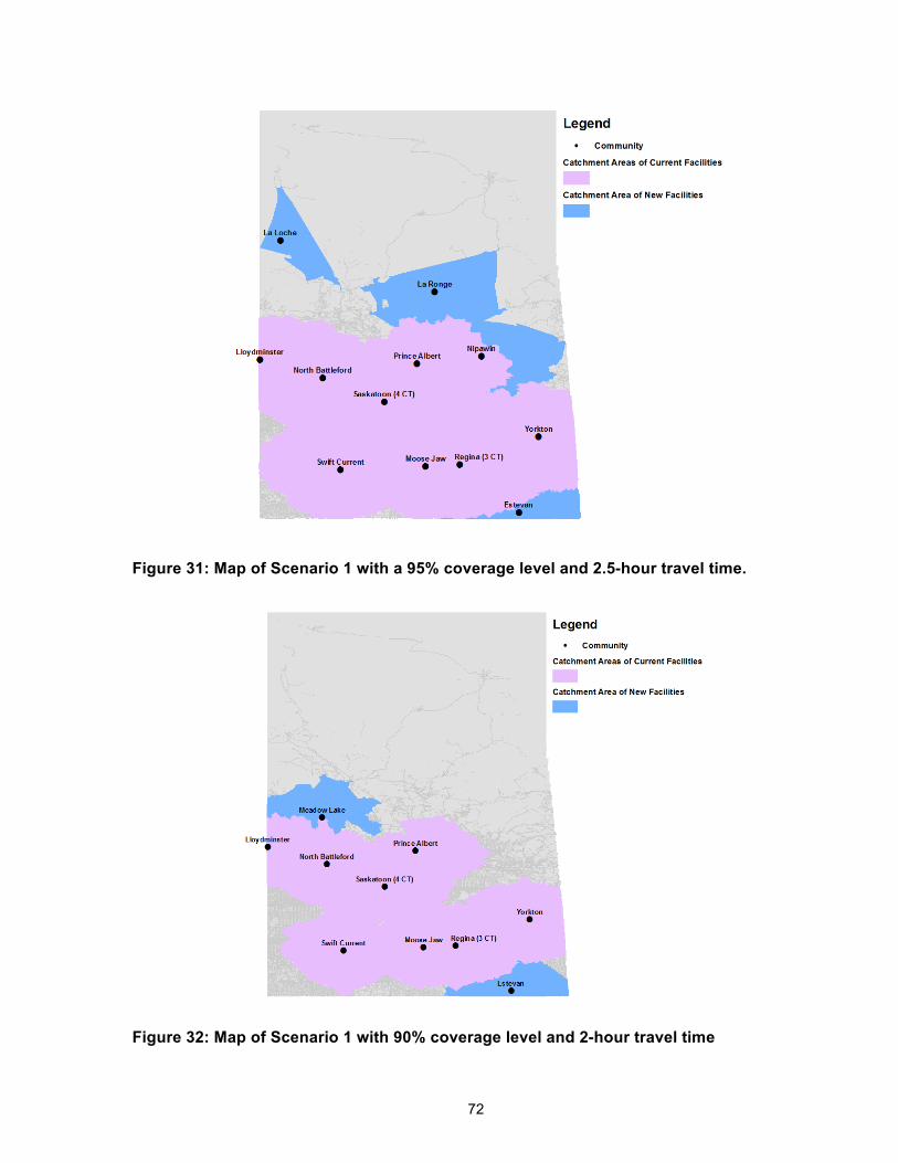
72

Figure 31: Map of Scenario 1 with a 95% coverage level and 2.5-hour travel time.

Figure 32: Map of Scenario 1 with 90% coverage level and 2-hour travel time

73

Figure 33: Map of Scenario 1 with 90% coverage level and 1.5-hour travel time.

5.6.2. Scenario 2: Covering all provincial demand

For scenario 2, the aim was to gain a better understanding of how existing capacity can meet

the entire provincial demand. Therefore, all exams needed to be assigned to a facility and a

high maximum travel time (20.2 hours) allowed all CT resources to be pooled. Existing facilities

were sufficient to meet the provincial demand. See Figure 34 for the distribution of operating

hours. The cost of $157,428,363.50 over the planning horizon is the same as when there is an

85% coverage level with a 2.5 hour or 2 hour catchment area. These scenarios have the same

number of operating hours and have no new facilities or CT scanners, so non-capital costs are

similar and there are no capital costs.

74

Figure 34: Weekly operating hours for all CT facilities for Scenario 2.

5.6.3. Scenario 3: Green Field

For the third scenario, the model was run assuming that there were no existing facilities. In the

first year, the model places nine facilities with one scanner each. Figure 35 shows the nine

chosen facilities and the distribution of operating hours. In 2014, Weyburn and Prince Albert are

each assigned a second CT scanner. See Figure 36 for the reach of catchment areas.

Having 11 CT scanners at 9 facilities is less costly upfront than the current situation of 13 CT

scanners in 11 facilities. However, there are fewer operating hours and increased overtime than

in the base scenario, so the average non-capital costs each year are $60,546.01 more for the

green field scenario.

Therefore, most of the cost difference is due to the capital costs for purchasing the CT scanners

and opening the facilities. With the strategic placement of CT scanners, six fewer shifts are

needed for the same minimum coverage percentage.

 -­‐        

 200    

 400    

 600    

 800    

 1,000    

 1,200    

 1,400    

 1,600    

2013  

2014  

2015  

2016  

2017  

2018  

2019  

2020  

2021  

2022  

2023  

2024  

2025  

2026  

2027  

2028  

2029  

2030  

Weekly  Ope

ra9n

g  Ho

urs  

Yorkton  

Prince  Albert  

Lloydminster  

North  Baaleford  

Moose  Jaw    

Swid  Current  

Saskatoon  (SPH)  

Saskatoon  (SCH)  

Saskatoon  (RUH)  

Regina  (RGH)  

Regina  (PH)  

75

Figure 35: Weekly operating hours for all CT facilities for Scenario 3.

Figure 36: Map of chosen facilities and 2-hr catchment areas for the green field scenario.

-

200

400

600

800

1,000

1,200

1,400

2013

20

14

2015

20

16

2017

20

18

2019

20

20

2021

20

22

2023

20

24

2025

20

26

2027

20

28

2029

20

30

Wee

kly

Ope

ratin

g H

ours

Prince Albert

North Battleford

Moose Jaw

Swift Current

Saskatoon (RUH)

Melville

Weyburn

Meadow Lake

Melfort

76

5.6.4. Sensitivity Analysis

A sensitivity analysis was run on the baseline scenario of 90% minimum coverage and a 2-hour

travel time to assess the impact of parameter changes. In all the scenarios, two facilities were

added except when demand varied; however, the location and opening year of the second

facility varied (Table 12). Overall, the model is not very sensitive to changes to the cost

parameters with similar operating hours. The model was sensitive to demand, overtime

surcharge, and exams per operating hour.

For the scenario of high demand, the shifts increased to 30 one year earlier in 2021 leading to

more shifts in total. For low demand, the increase to 30 shifts occurs one year later in 2023

resulting in fewer shifts in total. The total costs reflect this difference in number of shifts. When

the overtime surcharge is 100%, this changes the break-even point, more shifts are added to

reduce the number of overtime exams, and costs are slightly higher with an overtime surcharge

of 100%. The model is also sensitive to changes in the exams per operating hour. Figure 37

shows that as the number of exams per operating hour increases, fewer shifts are necessary,

but the total cost increases since each shift costs more.

Figure 37: Sensitivity analysis for exams per operating hour

-

100

200

300

400

500

600

163.00

163.20

163.40

163.60

163.80

164.00

164.20

2.49 2.61 3.10 3.93

Tota

l Num

ber o

f Shi

fts

Tota

l Cos

t (M

illio

ns)

Exams per Operating Hour

Total Cost Total Shift Number

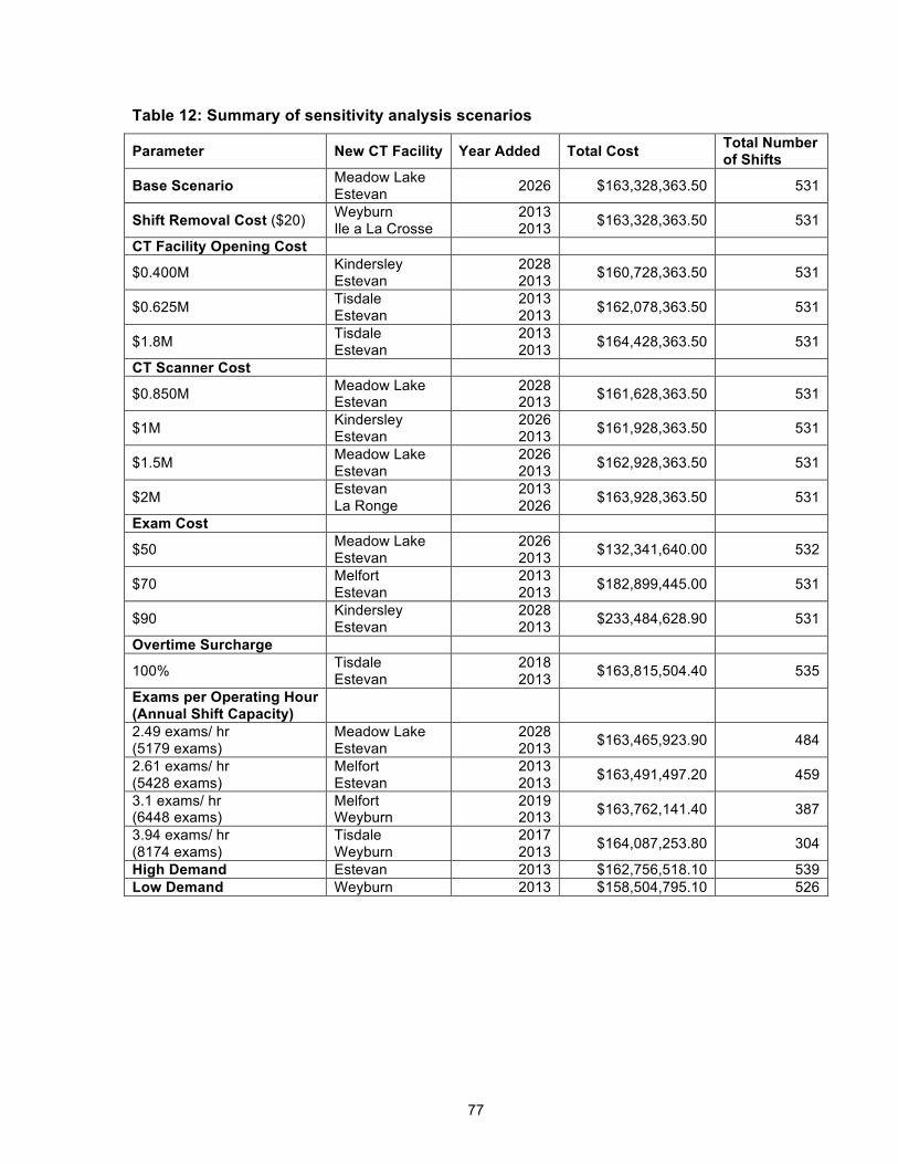
77

Table 12: Summary of sensitivity analysis scenarios

Parameter New CT Facility Year Added Total Cost Total Number of Shifts

Base Scenario Meadow Lake Estevan 2026 $163,328,363.50 531

Shift Removal Cost ($20) Weyburn Ile a La Crosse

2013 2013 $163,328,363.50 531

CT Facility Opening Cost

$0.400M Kindersley Estevan

2028 2013 $160,728,363.50 531

$0.625M Tisdale Estevan

2013 2013 $162,078,363.50 531

$1.8M Tisdale Estevan

2013 2013 $164,428,363.50 531

CT Scanner Cost

$0.850M Meadow Lake Estevan

2028 2013 $161,628,363.50 531

$1M Kindersley Estevan

2026 2013 $161,928,363.50 531

$1.5M Meadow Lake Estevan

2026 2013 $162,928,363.50 531

$2M Estevan La Ronge

2013 2026 $163,928,363.50 531

Exam Cost

$50 Meadow Lake Estevan

2026 2013 $132,341,640.00 532

$70 Melfort Estevan

2013 2013 $182,899,445.00 531

$90 Kindersley Estevan

2028 2013 $233,484,628.90 531

Overtime Surcharge

100% Tisdale Estevan

2018 2013 $163,815,504.40 535

Exams per Operating Hour (Annual Shift Capacity)

2.49 exams/ hr (5179 exams)

Meadow Lake Estevan

2028 2013 $163,465,923.90 484

2.61 exams/ hr (5428 exams)

Melfort Estevan

2013 2013 $163,491,497.20 459

3.1 exams/ hr (6448 exams)

Melfort Weyburn

2019 2013 $163,762,141.40 387

3.94 exams/ hr (8174 exams)

Tisdale Weyburn

2017 2013 $164,087,253.80 304

High Demand Estevan 2013 $162,756,518.10 539 Low Demand Weyburn 2013 $158,504,795.10 526

78

5.7. Discussion of Model

The purpose of the model was to provide some insight into CT capacity planning in order to

improve patient access by aligning CT supply with patient needs. The results of the model are

discussed in terms of increasing demand, increasing patient access, multiple possible

alternatives, and the base scenario.

If the minimum coverage percentage remains the same, but demand increases substantially

within the current catchment areas, then this results in longer operating hours and occasionally

additional CT scanners depending on existing levels of overtime and unused capacity in each

catchment area. This can be seen in the high demand scenario where the operating hours

increased by 1.5%. As the coverage percentage increases, new facilities are added to reach

more demand, raising the total cost. For example, when the travel time was 1.5hrs, the number

of new facilities increased from 1 to 7 as the coverage level rose from 80% to 90%. With the

new facilities came higher total costs.

The maximum travel time defines the hospital catchment areas and therefore is an important

driver in opening a new facility to increase the amount of covered demand. As the maximum

travel time increases from 1.5 hours to 2.5 hours, the cost difference between covering 90% of

the demand is $990,888.58 less on average each year. Most of the cost difference is from the

capital cost of opening new CT facilities since existing facilities do not need additional CT

scanners.

When the overall patient travel time decreases, so do the catchment areas. This reduces the

amount of covered demand and requires more facilities to be opened to meet the minimum

coverage level. More facilities cause the minimum number of required operating hours to

increase to meet the requirement of operating at least one shift per CT scanner. In the results,

the total number of operating hours required to meet all demand remains similar since operating

hours from existing facilities are shifted to the new facilities. However, it is possible that if

demand is more dispersed, many facilities are required to cover the demand. The number of

shifts and resulting capacity increases significantly because each facility must run for at least

one shift.

Furthermore, there are many alternative optimal solutions, which is not surprising given the

significant overlap between catchment areas. This allows decision makers to choose which

alternative optimal solution is most appropriate. The model is also not sensitive to changes in

79

the cost parameters. However, modifications to the demand, overtime surcharge, and exams

per operating hour did have a significant impact on number of new facilities, costs, and

operating hours.

On June 27, 2014, the province announced in a press release that a CT scanner would be

implemented in Estevan at St. Joseph’s Hospital by 2015 [76]. This matches our assumption

that candidate CT facilities should be district hospitals. Furthermore, the base scenario of a 2

hour travel time and 90% coverage level also places the next CT facility in Estevan. This is an

encouraging sign that the model is producing useful results.

80

5.8. Recommendations for Saskatchewan From the results, the main discussion around capacity planning in Saskatchewan centres on

pooling resources, capacity distribution and how the model can be used in the future.

Pooling Resources

The model assumes unassigned demand across the province will have access to any remaining

capacity. However, where patients go for their CT exams often depends on shorter wait times

and the location they are referred to by their physician. Figure 22 shows that a substantial

percentage of patients travel outside their health region for their exams. In 2011, 20% of visits

from Sunrise RHA and 27.8% of visits from Prince Albert Parkland Health Region traveled to

another health region and to a facility further away despite there being a facility in their health

region. By pooling the capacity of the existing system, Saskatchewan could reduce wait times at

some of their facilities.

Capacity Distribution

Capacity can be considered from two standpoints: theoretical maximum capacity and operating

hour capacity. The theoretical maximum capacity is based on how many exams can be done if

the CT scanner could be run and staffed for 24 hours a day, 7 days a week for the entire year.

The operating hour capacity is the number of exams which can be done each year during

regular operating hours.

Based on the theoretical maximum capacity, Saskatchewan has a substantial excess capacity,

because it could add more operating hours to accommodate increases in demand assuming the

human resources could be found. For example, by year 2030 only 25 out of 42 possible shifts of

operating hours (based on 3 shift maximum per CT scanner) are assigned to facilities. When

comparing the current operating hours to the suggested hours from the model, the excess

capacity is concentrated in certain areas.

In total, Saskatchewan currently has 804.5 hours of regular CT capacity per week. Regardless

of coverage percentage and maximum travel times ranging from 1.5 hrs to 2.5 hrs, the model

calculates that in 2013, 1000 operating hours are needed since there are 25 shifts and each

shift is 40 hours per week. This implies that there is currently an undersupply of operating hours

overall. However, the model also assumes that resources will be pooled to service any demand

beyond the minimum coverage percent. The undersupply by 195.5 hours and lack of pooling

81

resources needs to be further investigated to identify whether it is contributing to longer wait

times.

The distribution of the operating hours (Table 13) and additional factors need to be taken into

consideration. For example, in the base scenario, hospitals in Regina have substantially more

operating hours than what is calculated as necessary in the model. However, they also take in

patients from across the province, and out-of-region patients make up a third of the CT visits.

Furthermore, the model increased operating hours or added new facilities at Moose Jaw,

Estevan and Yorkton which have overlapping catchment areas with Regina.

Table 13: Current operating hours in comparison to average operating hours in model

using base scenario (90% coverage and 2 hour travel time) by facility

Health Region Community Hospital

Current Operating Hours per

Week

Model’s Operating Hours per

Week in 2013

Difference (Current -

Model)

Regina Qu'Appelle Regina Pasqua Hospital 119 80 39

Regina Qu'Appelle Regina Regina General

Hospital 182 160 22

Saskatoon Saskatoon Royal University Hospital 137 160 -23

Saskatoon Saskatoon Saskatoon City Hospital 62.5 80 -17.5

Saskatoon Saskatoon St. Paul's Hospital 50 80 -30

Sun Country Estevan St. Joseph's Hospital - 40 -40

Cypress Swift Current Cypress Regional Hospital

40 40 -

Five Hills Moose Jaw Moose Jaw Union Hospital 40 80 -40

Prairie North North Battleford

Battlefords Union Hospital 40 40 -

Prairie North Lloydminster Lloydminster Hospital 40 40 -

Prairie North Meadow Lake

Northwest Health Facility - Meadow Lake Hospital

- 40 -40

Prince Albert Parkland Prince Albert Victoria Hospital 54 120 -66

Sunrise Yorkton Yorkton Regional Health Centre

40 80 -40

Currently, Victoria Hospital in PAPHR has the longest wait times for all patient types (Table 8)

and the model assigns 120 hours per week. BUH and LH had the same number of operating

82

hours in the model and 2011 and they had the shortest wait times. However, Victoria Hospital

also does more exams per operating hour than BUH and LH (Figure 8). This information

suggests that more investigation is needed especially in terms of improved efficiency to avoid

increasing operating hours and staffing levels.

Rural hospitals tend to have staff working on multiple machines in a day such as the CTs and x-

rays. By having dedicated staff, CTs can run for the same number of operating hours, but

perform more exams. This may lower cost per exam since 92.2% of the cost is due to operating

and personnel expenses. However, if staff trained in CT exams are focusing less time on non-

CT exams, then more personnel may need to be hired for less expensive non-CT modalities

such as x-rays. For Victoria Hospital, this may mean that 56 hours per week is sufficient as long

as the staff spend more of their time doing CT exams.

Similarly, if the number of exams per operating hour increases, then this may also lower the

cost per exam since the majority of the costs are due to operations and personnel. In the

sensitivity analysis, it is assumed that the exam costs remain the same when the number of

exams per operating hour is higher so that only one parameter is changed at a time. However,

this overestimates the cost of operating a shift.

Given the potential advantages of pooling resources, a centralized booking system could be

investigated to reduce wait times. However, factors such as different staffing arrangements

need to be considered when looking at capacity.

Using the model

The input parameters for the model are based on many assumptions as detailed in Section

5.3.1. The model should be re-run with more accurate demand projections, which would be

affected by changes in the demand rate estimate. Parameters should also be updated for the

cost of a CT scanner, cost of renovation, and exam cost. From the sensitivity analysis, it is

known that the model results will not fluctuate substantially for these cost parameters, so

estimates can be used to achieve similar results if exact costs are lacking. The model is

intended for long-term planning and not emergency situations.

The model can also be forced to place facilities in certain locations with a specified number of

shifts. For example, the green field scenario did not place a CT scanner in Regina despite it

being one of the two major cities in Saskatchewan. The model does not know that Regina

General Hospital is a tertiary hospital which needs a CT scanner and other political factors.

83

Furthermore, it is beneficial to have more than the minimum number of CT scanners from the

green scenario for the inpatients and emergency patients at the additional hospitals. However,

the model can be forced to place CT scanners at certain facilities in the beginning. By forcing

the number of shifts, operating hours can also be concentrated in tertiary hospitals to reflect

existing patterns and identify the resulting number of operating hours required to meet demand

for the other facilities. Therefore, if the decision maker knows that all tertiary hospitals should

have a CT scanner and a certain number of operating hours, then this can be set in the model.

Being able to choose specific locations to open is also useful since there are multiple alternate

solutions covering similar percentages of demand at the same cost. For the scenario of a 2 hour

travel time and a minimum 90% coverage, there are slight differences in the maximum demand

covered based on 2012 calculations if the second new facility is located in Tisdale (93.5%),

Meadow Lake (93.3%), Melfort (93.3%), or Kindersley (93.1%). 93.3% demand covered is

approximately 1,325,303 people within two hours of a CT facility. This was calculated using the

average exams per 1000 population of 82.98. Since the costs in the model are estimated, it

might also be preferable to open a new facility at a slightly higher cost based on factors outside

the model’s scope. Furthermore, opening new facilities earlier had no cost implications based

on the model results, but improved patient access to CT scanners for more years. Opening new

facilities earlier at no extra cost may not be realistic given the costs associated with

administration and CT scanner replacement among other factors.

Incorporating mobile CT scanners

Improving rural access is one of the main goals of the thesis and all the new facilities selected

by the model are in the southern half of Saskatchewan. One way to reach the northern and

other rural areas is through mobile CT scanners. Saskatchewan previously used mobile CT

scanners in 2000 and it operated between Moose Jaw and Swift Current [77]. The aim was to

reduce travel times to Regina by bringing the CT scanner closer to patients. By 2004 and 2005,

permanent CT scanners were installed for Swift Current and Moose Jaw respectively.

A similar pattern can be used in other parts of Saskatchewan and incorporated into the model. A

set of candidate locations for the mobile scanner would be determined along with the expected

travel path. The model would then determine how much time was needed at each candidate

location (if any) and take into account moving costs each time. The costs associated with the

mobile CT scanner could be incorporated into the model’s objective function so that the capacity

of mobile CTs is taken into consideration when planning the permanent CT facilities.

84

Applying the model to other jurisdictions

This model can also be used outside of Saskatchewan in jurisdictions where planners care

about high population coverage and find the percent of demand within a catchment areas

aligned with their rural access standards. High population coverage tends to matter for areas

where healthcare is treated as a public service. Ontario and British Columbia use similar access

standards and can easily translate the model to their communities since they plan capacity

centrally.

In the United States, healthcare is privately delivered and 46.4% is funded by the government

[79]. However, due to the lack of centralized public planning for health services, the model

would be difficult to apply to the United States.

Although the model was developed for CT capacity planning, the model can be applied to

problems which share the same main characteristics of the high capital costs, high operating

shift costs, multiple machines at the same facility, lengthy planning horizon, and need for access

standards. Magnetic resonance imaging (MRI) facilities are another potential application

85

Chapter 6. Conclusions

The two main approaches for capacity planning research in health care services have been in

geography and operations research. In geography, various scenarios are run to assess the

impact on percent of demand within facility catchment area and resulting travel times. Many

capacitated covering models and plant location models have been developed in operations

research; however, assigning multiple facilities to the same site with shift allocation has not

been well explored. This thesis presents a method that combines an approach from geography

with a capacitated minimum covering model and uses Saskatchewan as a case study.

From Chapter 4, there was substantial variation in CT utilization and patient access metrics

between different CT facilities in Saskatchewan. After metrics were calculated by priority level

and patient type, not all differences between the facilities were explained. For CT utilization, a

more in-depth analysis of the specific facilities would be needed to understand the sources of

the variation. In terms of access, there are clear differences between rural and urban CSDs.

Mean travel times are also three times longer in rural areas than in areas with medium sized

populations. Differences in patient access and patient utilization are likely linked to travel time. A

regression model could be developed to identify which geographic and socio-demographic

factors contribute most to variation in patient utilization.

Through Chapter 5, potential new facilities, trends, and capacity distribution are better

understood. The model determined that Estevan should be the next CT facility in the base

scenario. The Ministry of Health in Saskatchewan [76] also chose Estevan has the next CT

facility and while decisions on where to locate new CT facilities are subject to many factors such

as politics this is an encouraging result. There are many alternative options for the second new

facility and the model can be re-run to determine the potential impact of the preferred locations.

Similarly, the number of shifts and the associated number of operating hours can be set in the

model for preferred locations. Re-running the model will recalculate the necessary number of

operating hours at the remaining facilitates. However, these results assume that the parameters

were accurate and the model should be re-run with when parameter values change.

For capacity, Saskatchewan has slightly less capacity than demand based on the number of

operating hours. Hospitals in Regina and Saskatoon have the most number of operating hours.

For Prince Albert, more work is necessary to determine if operating hours should be expanded,

the percent of time staff dedicate to CT could be increased, or existing processes can be more

86

efficient to prevent the need to expand operating hours. A provincial centralized booking system

could be considered to pool resources from all facilities and reduce wait times.

Furthermore, the model should be used as a tool in the decision making process to explore

different options. For example, a decision maker may want to know the magnitude of impact a

parameter will have on cost to the system. The model can be run multiple times with different

combinations of parameter values to assess the sensitivity of the results and the range of

impact on cost, capacity, and patient access.

To improve the model, a few model extensions could be considered for location-specific

parameters, CT scanner replacement, and closest facility assignment:

• The model assumed that each facility location would have the same opening costs, but

from CIHI [1] and Saskatchewan’s Ministry of Health press releases [69 - 73], the cost to

renovate a facility ranged from $0.400M to $1.8M. Furthermore, depending on the

staffing levels and other factors, facilities will differ in the number of exams per operating

hour. Given that the majority of the cost differences to improve coverage were the result

of capital expenditures and the model was sensitive to the number of exams per

operating hour, having location specific CT facility parameters could substantially

change the model results.

• CT scanners in Saskatchewan have been replaced after a decade or more (Table 3).

The capital costs associated with CT scanner replacement could be added to the model,

which may delay opening a new CT facility to avoid replacement costs.

• In the formulation, only a minimum percent of demand needs to be within a maximum

travel time. The remaining percent of demand is fulfilled, but has no patient travel time

restriction. To further improve rural access to CT scanners, travel time could be limited

by assigning demand to the next closest facility outside the maximum travel time.

The model was developed for CT capacity planning; however, the main characteristics are high

capital costs, high operating shift costs, multiple machines at the same facility, lengthy planning

horizon, and need for access standards. Another potential application is capacity planning for

magnetic resonance imaging facilities. Although this research provides insight into capacity

planning and opportunities for improving patient access and CT utilization, more research is

needed to have a complete understanding of factors affecting utilization and access.

87

References

[1] Canadian Institute for Health Information, "Medical Imaging in Canada ," Canadian Institute

for Health Information, Ottawa, 2008.

[2] Organisation for Economic Co-operation and Development, "OECD Health Data: Key

Tables from OECD," 2013.

[3] Health Canada. (2004) First Minister's Meeting on the Future of Health Care 2004. [Online].

http://www.hc-sc.gc.ca/hcs-sss/delivery-prestation/fptcollab/2004-fmm-rpm/index-eng.php

[4] Saskatchewan Health. (2013, Dec.) Computed Tomography (CT) Wait Times. [Online].

http://www.health.gov.sk.ca/diagnostic-imaging-ct-wait-times

[5] Government of Saskatchewan. (2013, Dec.) Saskatchewan Population Report. [Online].

http://www.stats.gov.sk.ca/stats/population/Censuspop2011.pdf

[6] Larson DB, Johnson LW, Schnell BM, Salisbury SR, Forman HP, "National Trends in CT

Use in the Emergency Department," Radiology, vol. 258, no. 1, pp. 164-173, 2011.

[7] Bhargavan M, Sunshine JH, "Utilization of Radiology Services in the United States: Levels

and Trends in Modalities, Regions, and Populations.," Radiology, vol. 234, pp. 824 – 832,

2005.

[8] Parker L, Levin DC, Frangos A, Rao VM, "Geographic Variation in the Utilization of

Noninvasive Diagnostic Imaging: National Medicare Data, 1998-2007," American Journal of

Roentgenology, vol. 194, no. 4, pp. 1034-1039, 2010.

[9] Kung PT, Tsai WC, Yaung CL, Liao KP, "Determinants of computed tomography and

magnetic resonance imaging utilization in Taiwan," International Journal of Technology

Assessment in Health Care, vol. 21, no. 1, pp. 81-88, 2005.

[10] Smith-Bindman R, Miglioretti DL, Larson EB., "Rising Use of Diagnostic Medical Imaging in

a Large Integrated Health System," Health Affairs, vol. 27, no. 6, pp. 1491-1502, 2008.

88

[11] Agarwal R, Bergey M, Sonnad S, Butowsky H, Bhargavan M, Bleshman MH, "Inpatient CT

and MRI Utilization: Trends in the Academic Hospital Setting," Am Coll Radiol, vol. 7, pp.

949-955, 2010.

[12] Matin A, Bates DW, Sussman A, Ros P, Hanson R, Khorasani R, "Inpatient Radiology

Utilization: Trends over the Past Decade," American Journal of Roentgenology., vol. 186,

pp. 7-11, 2006.

[13] Gazelle GS et al., "Utilization of Diagnostic Medical Imaging: Comparison of Radiologist

Referral versus Same-Specialty Referral," Radiology, vol. 245, no. 2, pp. 517-522 , 2007.

[14] Hillman BJ and Goldsmith J, "Imaging: the self-referral boom and the ongoing search for

effective policies to contain it," Health Affairs, vol. 29, no. 12, pp. 2231-2236, 2010.

[15] Gazelle GS, Halpern EF, Ryan HS, and Tramontano AC , "Utilization of Diagnostic Medical

Imaging: Comparison of Radiologist Referral versus Same-Specialty Referral ," vol. 245,

no. 2, pp. 517-522, 2007.

[16] Lee J, Kirschner J, Pawa S, Wiener DE, Newman DH, Shah K, "Computed Tomography

Use in the Adult Emergency Department of an Academic Urban Hospital From 2001 to

2007," Annals of Emergency Medicine, vol. 56, no. 6, pp. 591 – 596.e1, 2010.

[17] Oh HY, Kim EY, Cho J, Yang HK, Kim KH, Kim HS, Choi HY, "Trends of CT Use in the

Adult Emergency Department in a Tertiary Academic Hospital of Korea during 2001 –

2010," Korean Journal of Radiology, vol. 13, no. 5, pp. 536-540, 2012.

[18] Canadian Institute for Health Information. (2013) Medical Imaging in Canada 2012.

[Online]. http://www.cihi.ca/CIHI-ext-portal/pdf/internet/MIT_SUMMARY_2012_en

[19] Arcury TA, Preissier JS, Gesler WM, Powers JM, "Access to transportation and health care

utilization in a rural region," Journal of Rural Health, vol. 21, no. 1, pp. 31-38, 2005.

[20] Joseph AE, Boeckh JL, "Locational variation in mental health care utilization dependent

upon diagnosis: a Canadian example," Soc. Sci. Med., vol. 15, no. D, pp. 395-404, 1981.

[21] Nemet GF, Bailey AJ, "Distance and health care utilization among the rural elderly," Social

89

Science and Medicine, vol. 50, pp. 1197-1208, 2000.

[22] Stensland J, Akamigbo A, Glass D, Zabinski D, "Rural and urban Medicare beneficiaries

use remarkably similar amounts of health care services.," Health Affairs, vol. 32, no. 11, pp.

2040-2046, 2013.

[23] Chan L, Hart G, Goodman DC, "Geographic access to health care for rural Medicare

beneficiaries," National Rural Health Association, vol. 22, no. 2, pp. 140-146, 2006.

[24] Rao VM, Parker L, Levin DC, Sunshine J, Bushee G, "Use trends and geographic variation

in neuroimaging: Nationwide Medicare data for 1993 and 1998," AJNR Am J Neuroradiol,

vol. 22, pp. 1643-1649, 2001.

[25] Garg PP, Landrum MB, Normand SL, Ayanian JZ, Hauptman PJ, Ryan TJ, McNeil BJ,

Guadagnoli E, "Understanding individual and small area variation in the underuse of

coronary angiography following acute myocardial infarction.," Med Care, vol. 40, no. 7, pp.

614-626, 2002.

[26] Lysdahl KB, Borretzen I, "Geographical variation in radiological services: a nationwide

survey.," BMC Health Services Research, vol. 7, no. 21, 2007.

[27] Laupacis A, Pryzbysz R, Keller MA, "Access to Health Services in Ontario: ICES Atlas - CT

and MRI Scanning," 2005.

[28] Szczepura A, Clark M, "Creating a strategic management plan for magnetic resonance

imaging (MRI) provision.," Health Policy, vol. 53, pp. 91-104, 2000.

[29] Bach L, Hoberg R, "A planning model for regional systems of CT scanners," Socio-Econ

Plan. Sci, vol. 19, no. 3, pp. 189-199, 1985.

[30] Greenwald HP, Woodward JM, Berg DH, "Transportation or CT Scanners: A Theory and

Method of Health Resources Allocation.," Health Services Research, vol. 14, no. 3, pp.

207-219, 1979.

[31] Wang F, Luo W, "Measure of spatial accessibility to health care in a GIS environment:

synthesis and a case study in the Chicago region.," Environment and Planning B: Planning

and Design, vol. 30, pp. 865 - 884, 2003.

90

[32] Schurman N, Fiedler RS, Grzybowski SCW, Grund D, "Defining rational hospital

catchments for non-urban areas based on travel-time," International Journal of Health

Geographics, vol. 5, no. 43, 2006.

[33] ReVelle C, Marks D, Liebman JC, "An analysis of private and public sector location

models," Management Science., vol. 16, no. 11, pp. 692-707, 1970.

[34] Daskin MS, Dean LK, "Location of Health Care Facilities, Chapter 3," in Handbook of

OR/MS in Health Care: A Handbook of Methods and Applications., 2004, pp. 43-76.

[35] Brandeau ML, Chiu SS, "An overview of representative problems in location research.,"

Management Science, vol. 35, no. 6, pp. 645-674, 1989.

[36] Toregas C, Swain R, ReVelle C, Bergman L, "The location of emergency service facilities,"

Operations Research, vol. 19, no. 6, pp. 1363-1373, 1971.

[37] Datta S, Bandyopadhyay R, "An application of OR in micro-level planning in India,"

Computers and Operations Research, vol. 20, no. 2, pp. 121-132, 1993.

[38] Ren X, Chen J, Guo G, Cai W, "The application of the maximal coverage and partial

coverage model in the shelter location problem. Critical issues in transportation systems

planning, development and management," pp. 1472-1478.

[39] Zhu J, Liu D, Huang J, Han J, "Determining storage locations and capacities for emergency

response.," in 9th International Symposium on Operations Research and Its Applications,

Chengdu-Jiushaigou, China., 2010, pp. 262-269.

[40] Owen SH, Daskin MS, "Strategic facility location: A review," European Journal of

Operational Research, vol. 111, no. 3, pp. 423-447, 1998.

[41] Schilling DA, "Dynamic location modelling for public-sector facilities: a multicriteria

approach.," Decision Sciences, vol. 11, pp. 714-724, 1980.

[42] Jia H, Ordonez F, Dessouky MM, "A modeling framework for facility location of medical

services for large-scale emergencies," IIE Transactions, vol. 39, no. 1, pp. 41-55, 2007.

91

[43] Arabani AB, Farahani RZ, "Facility location dynamics: an overview of classifications and

applications," Computers and Industrial Engineering., vol. 62, pp. 408-420, 2012.

[44] ReVelle CS, Laporte G., "The plant location problem: new models and research

prospects.," Operations Research, vol. 44, no. 6, pp. 864-874, 1996.

[45] Wesolowsky GO, Truscott WG, "The multi-period location-allocation problem with

relocation of facilities," Management Science, vol. 22, no. 1, pp. 57-65, 1975.

[46] Rosenberg MW, "Locating small scale public facilities," Socio-Econ Plan. Sci., vol. 18, no.

3, pp. 151-158, 1984.

[47] Holmes J, Williams FB, Brown LA, "Facility location under a maximum travel restriction: An

example using day care facilities," Geographical Analysis, vol. 4, no. 3, pp. 258-266, 1972.

[48] Lee SM, Green GI, Kim CS, "A multiple criteria model for the location-allocation problem,"

Computers and Operations Research, vol. 8, pp. 1-8, 1981.

[49] Min H, "The dynamic expansion and relocation of capacitated public facilities: A multi-

objective approach," Computers and Operations Research, vol. 15, no. 3, pp. 243-252,

1986.

[50] Luss H, "Operations research and capacity expansion problems: A survey.," Operations

Research, vol. 30, no. 5, pp. 907-947, 1982.

[51] Murray AT, Gerrard RA, "Capacitated Service and Regional Constraints in Location-

Allocation Modelling," Location Science, vol. 5, no. 2, pp. 103-118, 1997.

[52] Ghiani G, Guerriero F, Musmanno R, "The capacitated plant location problem with multiple

facilities in the same site," Computers and Operations Research, vol. 29, pp. 1903-1912,

2002.

[53] Church RL, "The regionally constrained p-median problem," Geographical Analysis, vol. 22,

no. 1, pp. 22-32, 1990.

[54] Wu LY, Zhang XS, Zhang JL, "Capacitated facility location problem with general setup

92

cost," Computers & Operations Research, vol. 33, no. 5, pp. 1226-1241, 2006.

[55] Statistics Canada. (2014) Table 052-0005 - Projected population, by projection scenario,

age and sex, as of July 1, Canada, provinces and territories, annual (persons). [Online].

http://www5.statcan.gc.ca/cansim/a26?lang=eng&retrLang=eng&id=0520005&paSer=&patt

ern=&stByVal=1&p1=1&p2=37&tabMode=dataTable&csid=#F1

[56] Statistics Canada. (2006) Postal Code Conversion File.

[57] Esri. (2013) Universal Transverse Mercator. [Online].

http://help.arcgis.com/en/arcgisdesktop/10.0/help/index.html#/Universal_Transverse_Merca

tor/003r00000049000000/

[58] Environmental Systems Research Institute. (2011) ArcGIS Desktop: Release 10.2.

[59] Neuman CDG. (2007) Index of /~cneuman/mgtsc461/Lectures/Lecture 1 Sep 09. [Online].

http://www.ualberta.ca/~cneuman/mgtsc461/Lectures/Lecture%201%20Sep%2009/

[60] Saskatchewan Ministry of Health. (2013) Ministry of Health Covered Population 2013:

Notice to Readers. [Online]. http://population.health.gov.sk.ca/NoticetoReaders2013.htm

[61] Statistics Canada. (2012, May) Census release topics and dates. [Online].

http://www12.statcan.gc.ca/census-recensement/2011/rt-td/index-eng.cfm

[62] Statistics Canada, "Postal Code Conversion File Reference Guide," Catalogue no. 92-154-

G, 2013.

[63] Goel V, Williams JI, Anderson GM, Blackstien-Hirsch P, Fooks C, Naylor CD (eds),

"Patterns of Health Care in Ontario. The ICES Practice Atlas. 2nd edition," Canadian

Medical Association, Ottawa, 1996.

[64] Boone JM, Brunberg JA, "Computed Tomography Use in Tertiary Care University Hospital,"

Am Coll Radiol, vol. 5, pp. 132-138, 2008.

[65] British Columbia's Ministries of Health Services and Health Planning, "Standards of

accessibility and guidelines for provision of sustainable acute care services by health

authorities," 2002.

93

[66] Ontario's Ministry of Health and Long-Term Care, "Rural and Northern Health Care

Framework/Plan - Stage 1 Report," 2011.

[67] Mettler FA et al., "CT scanning: patterns of use and dose," J. Radiol. Prot, vol. 20, pp. 353-

359, 2000.

[68] Goldman LW, "Principles of CT: Multislice CT," Journal of Nuclear Medicine Technology,

vol. 36, pp. 57-68, May 2008.

[69] Government of Saskatchewan. (2011, June) R-8.2 Reg 6 - The Facility Designation

Regulations. [Online]. http://www.publications.gov.sk.ca/details.cfm?p=11559

[70] Government of Saskatchewan. (2006, March) CT scanner opens in Lloydminster. [Online].

http://www.gov.sk.ca/news?newsId=2ded8682-2377-4599-8560-5fd9742038ef

[71] Government of Saskatchewan. (2005, December) CT scanner opens in Saskatoon.

[Online]. http://www.gov.sk.ca/news?newsId=fe3630fb-83be-4dad-8bd3-ee87da700688

[72] Government of Saskatchewan. (2006, March) Prince Albert opens new CT scanner.

[Online]. http://www.gov.sk.ca/news?newsId=e6f4bb90-9e29-4864-b4b8-6284b739bdc5

[73] Government of Saskatchewan. (2005, January) CT service begins in Sunrise Health

Region. [Online]. http://www.gov.sk.ca/news?newsId=9ffd12aa-3dcc-49ab-8838-

a325523103c5

[74] Government of Saskatchewan. (2006, January) CT service officially opens in the

Battlefords. [Online]. http://www.gov.sk.ca/news?newsId=599bdced-4c1a-45da-97ac-

506a4823a1b7

[75] ECRI Institute. (2012) CT Scanning Systems. [Online]. https://www.ecri.org/ctscan

[76] Canadian Institute for Health Information, "Hospital Births in Canada: A Focus on Women

Living in Rural and Remote Areas," 2013.

[77] Government of Saskatchewan. (2014, June) CT Scanner Will Enhance Diagnostic Services

for Southeast Saskatchewan. [Online]. https://www.saskatchewan.ca/government/news-

94

and-media/2014/june/27/ct-scanner-estevan

[78] Government of Saskatchewan. (2000, March) Moose Jaw introduces mobile CT scan.

[Online]. http://www.gov.sk.ca/news?newsId=4807a2b8-c7be-4ab9-bfa4-4af4296ad197

[79] The World Bank. (2014, Nov) 2.15 World Development Indicators: Health Systems.

[Online]. wdi.worldbankorg/table/2.15

95

Appendix A : Data Fields Provided

Table 14: Data fields provided by health region

Health Region Data Fields All Health Regions Facility

Patient Identifier (Visit Identifier for SHR and RQHR) Age Sex Postal Code Exam Date Order procedure

Prairie North RHA Completed Volume Room/Bed Ordered Date and Time (not accurate) Transcribed Date and Time Final Report Date and Time Radiologist Order Physician Priority

Cypress RHA Completed Volume Patient Location Final Report Date and Time Radiologist Order Physician Priority Patient Type

Five Hills RHA Completed Volume Ordered Date and Time (not accurate) Transcribed Date and Time Final Report Date and Time Radiologist Order Physician Priority Patient Type

Sunrise RHA Ordered Date and Time (not accurate) Transcribed Date and Time Final Report Date and Time Radiologist Order Physician Priority Patient Type Detailed Procedure Row Count

Prince Albert Parkland RHA Patient Location Ordered Date and Time (not accurate) Transcribed Date and Time Final Report Date and Time Radiologist Order Physician

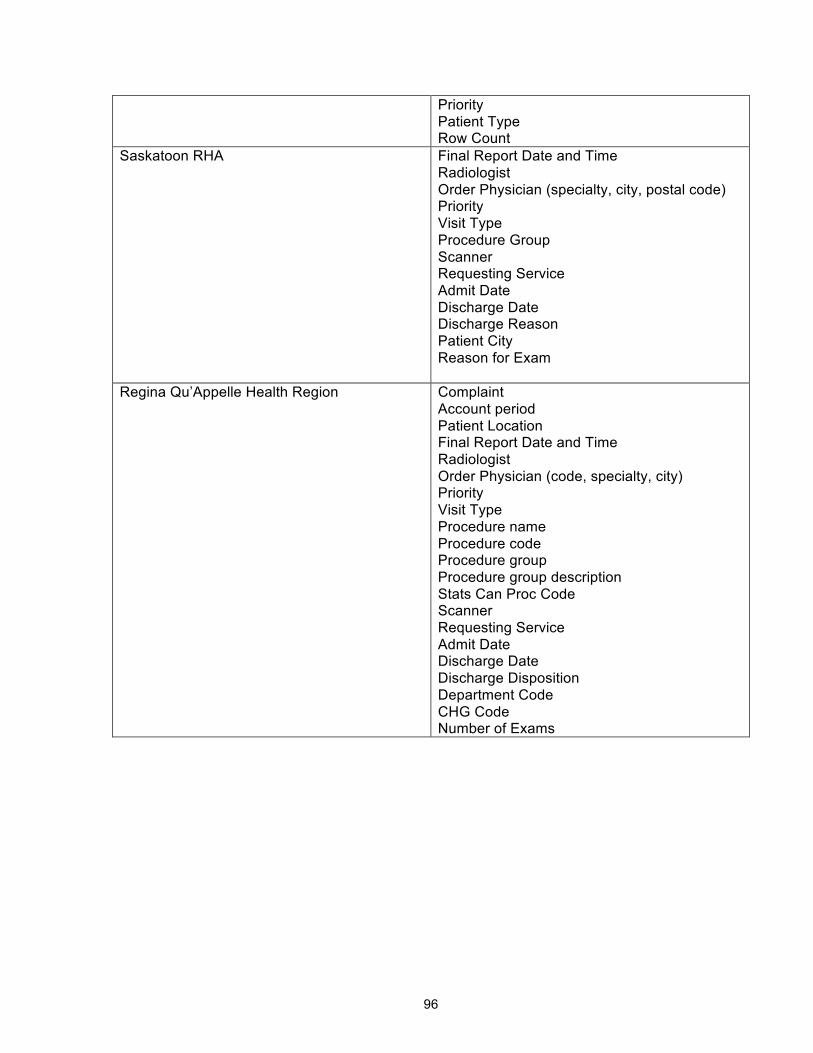
96

Priority Patient Type Row Count

Saskatoon RHA Final Report Date and Time Radiologist Order Physician (specialty, city, postal code) Priority Visit Type Procedure Group Scanner Requesting Service Admit Date Discharge Date Discharge Reason Patient City Reason for Exam

Regina Qu’Appelle Health Region Complaint Account period Patient Location Final Report Date and Time Radiologist Order Physician (code, specialty, city) Priority Visit Type Procedure name Procedure code Procedure group Procedure group description Stats Can Proc Code Scanner Requesting Service Admit Date Discharge Date Discharge Disposition Department Code CHG Code Number of Exams

97

Appendix B : Population Growth Rates

Table 15: Population projection based on sex and age group with growth scenario M1.

Sex   Male   Female  Age  Cohort   0-­‐19   20-­‐39   40-­‐59   60-­‐79   80+   0-­‐19   20-­‐39   40-­‐59   60-­‐79   80+  Year  

                   2012   1.0122   1.0429   1.0071   1.0320   1.0076   1.0144   1.0325   1.0056   1.0215   1.0027  2013   1.0091   1.0392   1.0027   1.0327   1.0040   1.0125   1.0282   1.0026   1.0267   0.9987  2014   1.0141   1.0313   1.0025   1.0361   1.0022   1.0160   1.0263   0.9997   1.0301   0.9980  2015   1.0083   1.0031   0.9940   1.0414   1.0052   1.0102   1.0053   0.9930   1.0354   0.9935  2016   1.0095   1.0006   0.9960   1.0365   1.0156   1.0122   1.0020   0.9951   1.0363   0.9967  2017   1.0115   0.9994   0.9959   1.0384   1.0000   1.0121   1.0020   0.9958   1.0319   0.9967  2018   1.0134   0.9951   0.9966   1.0380   1.0103   1.0140   1.0007   0.9957   1.0319   1.0000  2019   1.0132   0.9957   0.9966   1.0366   1.0152   1.0131   0.9987   0.9964   1.0329   1.0033  2020   1.0124   0.9950   0.9986   1.0344   1.0100   1.0123   0.9987   0.9964   1.0309   0.9967  2021   1.0129   0.9913   0.9993   1.0332   1.0149   1.0135   0.9961   1.0000   1.0263   1.0033  2022   1.0127   0.9924   1.0021   1.0286   1.0146   1.0126   0.9921   1.0036   1.0265   1.0098  2023   1.0107   0.9924   1.0000   1.0304   1.0288   1.0131   0.9908   1.0043   1.0267   1.0130  2024   1.0093   0.9917   1.0055   1.0236   1.0234   1.0091   0.9920   1.0050   1.0235   1.0096  2025   1.0092   0.9916   1.0075   1.0181   1.0365   1.0096   0.9919   1.0092   1.0197   1.0159  2026   1.0079   0.9929   1.0121   1.0129   1.0352   1.0083   0.9932   1.0134   1.0105   1.0250  2027   1.0054   0.9961   1.0120   1.0048   1.0553   1.0051   0.9959   1.0139   1.0032   1.0396  2028   1.0042   0.9993   1.0112   1.0048   1.0565   1.0038   0.9993   1.0151   1.0024   1.0352  2029   1.0030   1.0007   1.0111   1.0047   1.0496   1.0031   0.9973   1.0121   1.0032   1.0397  2030   1.0018   0.9987   1.0116   1.0024   1.0545   1.0025   1.0000   1.0127   1.0039   1.0381  2031   1.0018   1.0013   1.0089   1.0039   1.0517   1.0025   1.0000   1.0105   1.0016   1.0341  2032   1.0024   1.0020   1.0088   1.0008   1.0492   1.0012   1.0034   1.0085   1.0016   1.0406  2033   1.0018   1.0020   1.0094   1.0000   1.0531   1.0019   1.0041   1.0090   1.0000   1.0439  

Table 16: Population projection based on sex and age group with growth scenario L.

Sex   Male   Female  Age  Cohort   0-­‐19   20-­‐39   40-­‐59   60-­‐79   80+   0-­‐19   20-­‐39   40-­‐59   60-­‐79   80+  Year  

                   2012   1.0122   1.0429   1.0071   1.0320   1.0076   1.0144   1.0325   1.0056   1.0215   1.0027  2013   1.0091   1.0392   1.0027   1.0327   1.0040   1.0125   1.0282   1.0026   1.0267   0.9987  2014   1.0141   1.0313   1.0025   1.0361   1.0022   1.0160   1.0263   0.9997   1.0301   0.9980  2015   1.0048   1.0006   0.9926   1.0414   1.0052   1.0065   1.0033   0.9930   1.0354   0.9903  2016   1.0062   0.9981   0.9960   1.0354   1.0156   1.0101   1.0000   0.9937   1.0342   0.9967  2017   1.0075   0.9969   0.9939   1.0374   0.9949   1.0086   0.9987   0.9950   1.0330   1.0000  

98

2018   1.0095   0.9919   0.9952   1.0370   1.0103   1.0071   0.9974   0.9943   1.0300   0.9967  2019   1.0074   0.9931   0.9945   1.0357   1.0051   1.0085   0.9967   0.9943   1.0320   0.9967  2020   1.0066   0.9912   0.9959   1.0335   1.0203   1.0063   0.9954   0.9942   1.0310   1.0000  2021   1.0053   0.9885   0.9972   1.0315   1.0100   1.0076   0.9914   0.9985   1.0264   1.0033  2022   1.0046   0.9897   0.9986   1.0305   1.0148   1.0055   0.9886   0.9993   1.0266   1.0033  2023   1.0046   0.9883   0.9979   1.0279   1.0194   1.0048   0.9864   1.0022   1.0251   1.0099  2024   1.0007   0.9882   1.0021   1.0221   1.0286   1.0020   0.9890   1.0029   1.0219   1.0130  2025   1.0026   0.9880   1.0042   1.0183   1.0231   1.0014   0.9875   1.0058   1.0190   1.0129  2026   1.0000   0.9892   1.0083   1.0098   1.0407   1.0000   0.9887   1.0101   1.0089   1.0190  2027   0.9981   0.9932   1.0082   1.0048   1.0565   0.9980   0.9922   1.0114   1.0032   1.0374  2028   0.9948   0.9959   1.0088   1.0032   1.0453   0.9952   0.9957   1.0099   1.0016   1.0390  2029   0.9948   0.9972   1.0067   1.0024   1.0512   0.9952   0.9942   1.0091   1.0032   1.0347  2030   0.9947   0.9959   1.0067   1.0008   1.0487   0.9938   0.9949   1.0090   1.0008   1.0307  2031   0.9927   0.9972   1.0053   1.0024   1.0464   0.9938   0.9964   1.0068   1.0000   1.0352  2032   0.9940   0.9986   1.0053   1.0000   1.0512   0.9944   1.0000   1.0041   1.0000   1.0366  2033   0.9933   0.9993   1.0046   0.9976   1.0552   0.9930   1.0007   1.0041   0.9976   1.0429  

Table 17: Population projection based on sex and age group with growth scenario H.

Sex   Male   Female  Age  Cohort   0-­‐19   20-­‐39   40-­‐59   60-­‐79   80+   0-­‐19   20-­‐39   40-­‐59   60-­‐79   80+  Year  

                   2012   1.0122   1.0429   1.0071   1.0320   1.0076   1.0144   1.0325   1.0056   1.0215   1.0027  2013   1.0091   1.0392   1.0027   1.0327   1.0040   1.0125   1.0282   1.0026   1.0267   0.9987  2014   1.0141   1.0313   1.0025   1.0361   1.0022   1.0160   1.0263   0.9997   1.0301   0.9980  2015   1.0110   1.0056   0.9953   1.0390   1.0052   1.0116   1.0066   0.9937   1.0365   1.0000  2016   1.0136   1.0025   0.9960   1.0387   1.0156   1.0150   1.0039   0.9958   1.0352   0.9968  2017   1.0147   1.0012   0.9973   1.0383   1.0103   1.0176   1.0026   0.9965   1.0350   0.9967  2018   1.0192   0.9976   0.9980   1.0400   1.0102   1.0180   1.0032   0.9972   1.0308   1.0033  2019   1.0181   0.9975   0.9973   1.0365   1.0151   1.0191   1.0013   0.9964   1.0347   1.0033  2020   1.0191   0.9969   1.0000   1.0361   1.0099   1.0194   1.0013   0.9986   1.0299   1.0000  2021   1.0200   0.9951   1.0020   1.0349   1.0294   1.0203   0.9981   1.0014   1.0290   1.0097  2022   1.0196   0.9963   1.0034   1.0310   1.0190   1.0212   0.9948   1.0043   1.0282   1.0129  2023   1.0192   0.9963   1.0041   1.0301   1.0280   1.0195   0.9948   1.0064   1.0265   1.0190  2024   1.0171   0.9944   1.0074   1.0242   1.0273   1.0173   0.9954   1.0085   1.0250   1.0156  2025   1.0168   0.9956   1.0094   1.0220   1.0354   1.0170   0.9954   1.0112   1.0212   1.0123  2026   1.0154   0.9956   1.0139   1.0136   1.0427   1.0161   0.9961   1.0145   1.0127   1.0242  2027   1.0140   1.0000   1.0150   1.0063   1.0615   1.0129   0.9993   1.0164   1.0047   1.0533  2028   1.0111   1.0019   1.0148   1.0070   1.0618   1.0110   1.0020   1.0168   1.0031   1.0393  2029   1.0104   1.0032   1.0127   1.0054   1.0545   1.0115   1.0013   1.0145   1.0055   1.0405  2030   1.0103   1.0019   1.0144   1.0046   1.0586   1.0102   1.0020   1.0156   1.0047   1.0390  

99

2031   1.0102   1.0038   1.0117   1.0054   1.0489   1.0107   1.0033   1.0135   1.0039   1.0425  2032   1.0101   1.0031   1.0116   1.0038   1.0621   1.0094   1.0046   1.0127   1.0023   1.0432  2033   1.0100   1.0050   1.0115   1.0008   1.0585   1.0099   1.0065   1.0106   1.0000   1.0460  

100

Appendix C : Data Map

Table 18 through to Table 27 indicate the number of records which were used to calculate the

baseline statistics with different cuts of the data in the rest of the chapter. The number of

records changes due to missing data for certain fields. For certain calculations, the sample size

is dependent on the postal code. Table 18 breaks down the data based on postal code validity

and in-province/out-of-province and provides the total number of data points.

Table 18: CT exam data map based on postal code.

Number of Data Points

Total 586,386

Invalid/Missing postal codes 25

Out-of-province 18,680

In-province, invalid postal code 865

In-province, valid postal code 566,816

Table 19: Number of data points by facility and year

2000 2001 2002 2003 2004 2005 2006 2007 2008 2009 2010 2011 2012 2013

CRH 0 0 0 0 0 0 0 318 4244 4232 3758 3643 3457 896

MJU 0 0 0 0 0 0 0 0 0 656 5732 5747 5801 1801

VH 0 0 0 0 0 0 0 0 0 0 4980 6948 7153 8049

BUH 0 0 0 0 0 0 0 0 0 3718 4253 4079 4172 1017

LH 0 0 0 0 0 0 0 0 0 2489 3925 3603 3763 1030

PH 0 0 0 2596 2930 1961 3246 2100 2103 1956 2153 2014 437 0

RGH 0 0 0 8237 10759 10479 10562 9974 9765 8943 8737 10783 8210 0

RUH 10440 10992 11497 11318 13055 14911 15784 16087 17525 18779 17540 18785 7930 0

SCH 0 0 1046 6867 7093 7741 7742 7866 7788 9170 11126 12243 4972 0

SPH 0 0 0 6368 7082 7493 8273 9500 11542 11434 11039 10210 4180 0

YRH 0 0 0 0 0 0 0 0 0 0 477 3992 4006 5084

101

Table 20: Number of data points by priority level and facility in 2011

Priority Level

Facility 1 2 3 4

CRH 1280 647 642 1074

MJU 2597 716 1354 1080

VH 3377 1079 1716 776

BUH 1464 1149 1081 385

LH 1323 1042 988 250

YRHC 1805 765 869 553

Table 21: Number of data points by patient type and facility in 2011

Emergency Inpatient Outpatient

CRH 521 668 2454

MJU 1595 776 3376

VH 2410 669 3868

BUH 1038 474 2566

LH 924 498 2181

PH 58 456 1500

RGH 281 1682 8820

RUH 8539 4729 5517

SCH 1136 237 10870

SPH 2852 3020 4338

YRH 999 391 2602

102

Table 22: Number of data points which have exam time by facility in 2011.

Number of data points

CRH 20548

MJU 19737

VH 27130

BUH 17239

LH 14810

PH 21496

RGH 96449

RUH 184643

SCH 83654

SPH 87121

YRH 13559

Table 23: Number of data points by procedure group and facility in 2011

Head Spine Upper Extremity

Lower Extremity

Thorax Abdomen/ Pelvix

Miscellaneous

Vascular

CRH 1153 536 14 52 754 1155 199 145

MJU 1898 792 17 84 1008 1789 189 463

VH 2779 478 48 96 1305 2287 293 267

BUH 1469 468 22 78 656 1483 176 127

LH 1389 274 16 40 626 1212 84 243

PH 387 51 0 0 489 1025 62 0

103

RGH 2036 539 0 0 3074 4718 416 0

RUH 7244 1556 214 481 2821 4348 1 2120

SCH 2544 241 80 284 3680 4646 0 768

SPH 2117 195 18 98 1808 4102 12 1860

YRH 1234 369 21 42 996 1537 233 147

Table 24: Number of data points with report turnaround time by facility in 2011

Facility Data Points with Report Turnaround Time

CRH 20548

MJU 19737

VH 27130

BUH 17239

LH 14810

PH 21496

RGH 96449

RUH 184643

SCH 83654

SPH 87121

YRH 13559

Table 25: Number of visits in 2011 by facility.

Facility Count

Cypress 2340

FiveHills 3178

PAParkland 3687

104

BUH 2453

LH 2059

PASQUA 893

RGH 5450

RUH 4081

SCH 7349

SPH 3109

Sunrise 2475

Table 26: Number of visits by population centre and rural area classification in 2011

Population centre and rural area classification Number of Visits

Rural Area 1643

Small (1,000 – 29,999 pop.) 7061

Medium (30,000 - 99,999 pop.) 3539

Large Urban (100,000 or greater) 10610

Table 27: Number of visits by patient health region and CT facility in 2011.

CT Facility

Patient Health Region CRH MJUH VH BUH LH PH RGH RUH SCH SPH YRHC Athabasca Health Authority 0 0 1 0 67 0 0 60 10 13 0

Cypress RHA 3310 73 3 3 0 176 58 279 117 103 0

Five Hills RHA 46 5085 6 1 0 578 102 114 65 27 0

Heartland RHA 189 77 418 71 5 8 8 1282 849 645 0

Keewatin YatthÚ RHA 0 0 289 2 72 0 0 353 99 116 2

Kelsey Trail RHA 4 5 3 3 1209 39 6 958 623 581 41 Mamawetan Churchill River RHA 0 1 6 0 515 1 0 411 125 182 0

Prairie North RHA 0 4 3061 1382 12 2 3 1052 531 571 0 Prince Albert Parkland RHA 1 1 158 10 4740 21 7 1139 693 635 1

Regina Qu'Appelle RHA 24 175 10 0 13 7090 1326 227 93 53 75

105

Saskatoon RHA 7 24 43 6 159 164 21 12163 8770 7019 46

Sun Country RHA 1 211 0 1 4 1837 276 36 36 29 7

Sunrise RHA 0 5 3 6 7 748 184 250 153 130 3676

106

Appendix D : AMPL Files

AMPL Model Formulation File (.mod) set DEMAND:= 1..959; set CT:= 1..23; set TIME:= 1..19; set TIME_subset within TIME := 1..18; #1 less than TIME set; param Demand{DEMAND,TIME}; #Demandit = number of CT scans in area i in each year t param DemandTotal{TIME}; #DemandTotal param MinCoverage; #= Minimum percentage of total demand in Saskatchewan that must be covered param a{DEMAND,CT}; # = { 1 if CT demand in area i is within patient travel distance radius r of location j, 0 otherwise} param Capmax; #= maximum capacity allowed at a CT param CapShift; #= regular shift hours param CostOpen; #= cost of opening a new CT facility param CostCT; #= cost of adding a CT to an open facility param ExamCost; #= cost of an assigned overtime CT exam param MaxShift;#maximum number of shifts param OvertimeSurcharge; param ShiftRemovalCost; var DemandFraction{DEMAND,CT,TIME}>=0; #xijt = fraction of demand covered at location i by CT at location j at time t var CTDecision{CT,TIME} binary; #yjt = {1 if a new CT is placed in location j at time t, 0 otherwise} var CTTotal{CT,TIME} integer >=0; #Yjt To initialize the model: yj0 = number of current CTs at location j at time 0, Yjt = total number of CTs at location j at time t var CTnew{CT} binary; #zj = {1 if a new facility is placed at location j in any period, 0 otherwise} var CTover{CT,TIME} >=0; #assigned overtime exams var CTunder{CT,TIME} >=0; #assigned undertime exams var Shifts{CT,TIME} integer >=0; #shifts assigned to a facility var ShiftRemoved{CT,TIME} >=0 ; var ShiftAdded{CT,TIME} >=0 ; var AssignedDemand{CT,TIME}>=0; var UnassignedDemand{TIME} >=0; var UnassignedOver{TIME} >=0; #assigned overtime exams var UnassignedUnder{TIME} >=0; #assigned undertime exams #var CapOver{CT,TIME}>=0; minimize Cost: CostOpen*sum{j in CT}CTnew[j] + CostCT*sum{t in TIME_subset}sum{j in CT}CTDecision[j,t+1]+ ExamCost*OvertimeSurcharge*sum{t in TIME_subset}sum{j in CT}CTover[j,t+1] + ExamCost*OvertimeSurcharge*sum{t in TIME_subset}UnassignedOver[t+1]+ ExamCost*CapShift*sum{t in TIME_subset}sum{j in CT}Shifts[j,t+1]+ ShiftRemovalCost*sum{t in TIME_subset}sum{j in CT}ShiftRemoved[j,t+1];; subject to x1 {t in TIME_subset}: sum{i in DEMAND}sum{j in CT}DemandFraction[i,j,t+1]*Demand[i,t+1]>= MinCoverage*DemandTotal[t+1]; subject to x2 {t in TIME_subset}: DemandTotal[t+1]<= Capmax*sum{j in CT}CTTotal[j,t+1];

107

subject to x3 {j in CT, t in TIME_subset}: sum{i in DEMAND}DemandFraction[i,j,t+1]*Demand[i,t+1] = CapShift*Shifts[j,t+1] + CTover[j,t+1] - CTunder[j,t+1] ; subject to x4 {j in CT, t in TIME_subset}: CTover[j,t+1] <= Capmax*CTTotal[j,t+1]- CapShift*Shifts[j,t+1]; subject to x5 {i in DEMAND, j in CT, t in TIME_subset}: DemandFraction[i,j,t+1] <= a[i,j]*CTTotal[j,t+1]; subject to x6 {i in DEMAND, t in TIME_subset}: sum{j in CT}DemandFraction[i,j,t+1] <= 1; subject to x7 {j in CT, t in TIME_subset}: CTnew[j] >= CTDecision[j,t+1] - CTTotal[j,1]; subject to x8 {j in CT, t in TIME_subset}: CTTotal[j,t+1] = CTTotal[j,t] + CTDecision[j,t+1]; #limit to t >= 1 subject to x9 {j in CT, t in TIME_subset}: Shifts[j,t] - Shifts[j,t+1] = ShiftRemoved[j,t+1] - ShiftAdded[j,t+1]; subject to x10:CTTotal[1,1]=0; subject to x11:CTTotal[2,1]=0; subject to x12:CTTotal[3,1]=0; subject to x13:CTTotal[4,1]=0; subject to x14:CTTotal[5,1]=0; subject to x15:CTTotal[6,1]=0; subject to x16:CTTotal[7,1]=0; subject to x17:CTTotal[8,1]=0; subject to x18:CTTotal[9,1]=0; subject to x19:CTTotal[10,1]=0; subject to x20:CTTotal[11,1]=0; subject to x21:CTTotal[12,1]=0; subject to x22:CTTotal[13,1]=1; subject to x23:CTTotal[14,1]=2; subject to x24:CTTotal[15,1]=2; subject to x25:CTTotal[16,1]=1; subject to x26:CTTotal[17,1]=1; subject to x27:CTTotal[18,1]=1; subject to x28:CTTotal[19,1]=1; subject to x29:CTTotal[20,1]=1; subject to x30:CTTotal[21,1]=1; subject to x31:CTTotal[22,1]=1; subject to x32:CTTotal[23,1]=1; subject to x33{j in CT, t in TIME_subset}:Shifts[j,t+1]<= MaxShift*CTTotal[j,t+1]; subject to x34 {t in TIME_subset}:DemandTotal[t+1] - (sum{i in DEMAND}sum{j in CT}DemandFraction[i,j,t+1]*Demand[i,t+1]) = UnassignedDemand[t+1]; subject to x35 {t in TIME_subset}:UnassignedDemand[t+1] - sum{j in CT}CTunder[j,t+1] = UnassignedOver[t+1] - UnassignedUnder[t+1]; subject to x36{j in CT, t in TIME_subset}:Shifts[j,t+1]>= CTTotal[j,t+1]; AMPL Data File (Travel Time 2 hours and 90% coverage) param MinCoverage := 9.000000e-001; param Capmax := 24723; param CapShift := 4700; param CostOpen:= 1250000; param CostCT := 1700000; param ExamCost := 6.226000e+001;

108

param MaxShift := 3; param OvertimeSurcharge := 1.500000e+000; param ShiftRemovalCost:=100000; param Demand := 1 1 3.450769e+001 1 2 3.507199e+001 1 3 3.568170e+001 1 4 3.621902e+001 1 5 3.679340e+001 1 6 3.731274e+001 1 7 3.789408e+001 1 8 3.845858e+001 1 9 3.909870e+001 1 10 3.967275e+001 1 11 4.027297e+001 1 12 4.089807e+001 1 13 4.151963e+001 1 14 4.206922e+001 1 15 4.259477e+001 CONTINUED… param DemandTotal:= 1 1.178736e+005 2 1.197780e+005 3 1.218793e+005 4 1.239983e+005 5 1.263113e+005 6 1.284345e+005 7 1.308426e+005 8 1.334270e+005 9 1.357988e+005 10 1.382672e+005 11 1.407583e+005 12 1.436284e+005 13 1.461050e+005 14 1.486538e+005 15 1.509099e+005 16 1.531696e+005 17 1.554512e+005 18 1.577133e+005 19 1.600728e+005 ; param a default 0 := 364 1 1 385 1 1 386 1 1 387 1 1 388 1 1 389 1 1 390 1 1

109

391 1 1 392 1 1 396 1 1 397 1 1 398 1 1 399 1 1 400 1 1 401 1 1 402 1 1 403 1 1 404 1 1 405 1 1

CONTINUED

110

Appendix E : Metrics

Table 28: Percentage of patient’s by health region of origin for each CT Facility in 2011

Unm

atch

ed

Ath

abas

ca

Cyp

ress

Five

Hill

s

Hea

rtlan

d

Kee

wat

in Y

atth

é

Kel

sey

Trai

l

MC

R

Pra

irie

Nor

th

PA

PH

R

RQ

HR

Sas

kato

on

Sun

Cou

ntry

Sun

rise

CRH 0.77 - 90.3 1.54 6.84 - 0.13 - - - 0.30 0.13 - -

MJUH 0.94 - 1.70 86.0 1.70 - 0.09 - 0.09 0.03 3.87 0.16 5.35 0.06

VH 0.98 1.03 - - 0.05 0.95 25.74 7.21 0.24 61.62 0.08 1.95 0.05 0.08

LH 1.10 0.04 0.04 0.08 14.35 10.35 0.04 0.04 70.97 2.36 - 0.61 - -

BUH 61.00 - - 0.05 2.77 - - - 35.89 0.19 - - - 0.10

PH 1.12 - 1.34 4.37 0.22 - 0.22 - 0.11 0.34 71.11 0.67 11.87 8.62

RGH 0.72 - 1.21 4.59 0.06 - 0.22 0.02 0.02 0.04 70.81 1.43 15.39 5.50

RUH 0.54 0.27 1.47 0.61 7.65 1.27 5.76 1.47 5.46 6.37 0.83 66.67 0.15 1.47

SCH 0.39 0.11 0.83 0.57 7.32 0.78 4.86 0.95 4.12 5.35 0.87 72.25 0.31 1.28

SPH 0.45 0.06 1.00 0.39 7.17 0.71 6.37 1.67 4.79 5.56 0.71 69.73 0.19 1.19

YRHC 2.95 - - - - - 1.09 - - 0.04 2.02 1.05 0.16 92.69

111

Figure 38: Proportions of patient type by health region in 2011.

Table 29: Percent of outpatient visits that went to each CT facility from each health

region in 2011 based on the patient’s residential postal code.

CT HR Cy-

press FH

HR

PAP

HR PNRHA RQHR Saskatoon

Sun-

rise

CT Facility CRH MJU VH LH BUH PH RGH RUH SCH SPH YRH

Patient HR

Athabasca 0.0 0.0 63.3 1.7 0.0 0.0 0.0 18.3 13.3 3.3 0.0

Cypress 88.1 2.3 0.0 0.0 0.0 0.5 2.8 2.5 2.5 1.3 0.0

Five Hills 1.1 87.0 0.0 0.1 0.0 1.2 8.0 0.8 1.3 0.4 0.0

Heartland 9.4 3.2 0.1 20.7 3.3 0.1 0.2 18.3 31.6 13.1 0.0

Keewatin

Yatthé 0.0 0.0 8.3 60.5 0.0 0.0 0.0 12.4 13.6 5.2 0.0

14.3%  28.1%  

37.2%  25.6%  

2.6%  

30.4%   23.6%   25.6%  

17.8%  

13.4%  9.0%  

12.3%  

16.9%  

19.4%  

9.5%  16.0%  

67.9%  58.6%   53.9%  

62.1%  

80.5%  

50.3%  66.9%  

58.4%  

0%  

10%  

20%  

30%  

40%  

50%  

60%  

70%  

80%  

90%  

100%  

Cypress   Five  Hills   Prince  Albert  Parkland  

Prairie  North   Regina  Qu'Appelle  

Saskatoon   Sunrise   Province  

Emergency   InpaQent   OutpaQent  

112

Kelsey Trail 0.2 0.2 53.1 0.1 0.0 0.1 0.7 13.2 20.0 11.1 1.5

MCR 0.0 0.0 59.1 0.2 0.0 0.0 0.2 13.3 15.6 11.6 0.0

Prairie North 0.0 0.1 0.3 54.9 23.3 0.0 0.0 7.0 9.6 4.7 0.0

PAPHR 0.0 0.0 71.7 1.8 0.1 0.1 0.1 8.2 12.4 5.5 0.0

RQHR 0.1 2.6 0.1 0.0 0.0 13.2 80.4 0.7 1.3 0.5 1.0

Saskatoon 0.0 0.0 0.7 0.1 0.0 0.1 0.7 26.2 51.0 20.8 0.2

Sun Country 0.0 14.7 0.2 0.0 0.0 9.2 72.6 0.5 2.0 0.5 0.3

Sunrise 0.0 0.1 0.1 0.0 0.1 2.7 10.5 2.1 3.3 1.3 80.0

Table 30: Proportion of each procedure group by facility

Health Region Facility Head Spine

Upper Extremity

Lower Extremity Thorax

Abdo-men

Pelvis Misc. Vascular Cypress CRH 25.8% 12.6% 0.3% 1.1% 22.3% 30.7% 4.1% 3.2% FHHR MJUH 28.3% 12.3% 0.2% 1.2% 18.8% 29.6% 2.6% 7.1% PAPHR VH

31.7% 5.5% 0.4% 0.8% 20.2% 34.3% 3.0% 4.1% PNRHA BUH 30.7% 10.8% 0.4% 1.5% 17.6% 33.1% 3.3% 2.6%

LH 33.3% 7.0% 0.4% 0.9% 18.9% 31.9% 1.9% 5.9% RQHR PASQUA 19.2% 2.5% 0.0% 0.0% 24.3% 50.9% 3.1% 0.0%

RGH 19.0% 5.1% 0.0% 0.0% 28.5% 43.5% 3.8% 0.0% Saskatoon RUH 38.6% 8.3% 1.1% 2.6% 15.0% 23.1% 0.0% 11.3%

SCH 20.8% 2.0% 0.7% 2.3% 30.1% 37.9% 0.0% 6.3% SPH 20.7% 1.9% 0.2% 1.0% 17.7% 40.2% 0.1% 18.2%

Sunrise YRHC 23.3% 7.3% 0.4% 0.7% 25.9% 35.3% 4.0% 3.0%

113

Appendix F : Potential Facilities Table 31: List of potential facilities

Facility Name Kindersley & District Health Centre Melfort Hospital Tisdale Hospital Nipawin Hospital Northwest Health Facility - Meadow Lake Hospital Humboldt District Hospital St. Joseph's Hospital Weyburn General Hospital St. Peter's Hospital St. Joseph's Health Centre La Loche Health Centre La Ronge Health Centre Pasqua Hospital Regina General Hospital Royal University Hospital Saskatoon City Hospital St. Paul's Hospital Cypress Regional Hospital Moose Jaw Union Hospital Battlefords Union Hospital Lloydminster Hospital Victoria Hospital Yorkton Regional Health Centre