arX

iv:1

007.

1844

v2 [

mat

h-ph

] 1

5 Ju

l 201

0

Symplectic geometry of entanglement

Adam Sawicki1, Alan Huckleberry2, and Marek Kus1

1Center for Theoretical Physics, Polish Academy of Sciences

Al. Lotnikow 32/46, 02-668 Warszawa, Poland

2Fakultat fur Mathematik, Ruhr-Universitat Bochum,D-44780 Bochum, Germany

July 16, 2010

Abstract

We present a description of entanglement in composite quantum systems interms of symplectic geometry. We provide a symplectic characterization of setsof equally entangled states as orbits of group actions in the space of states. Inparticular, using Kostant-Sternberg theorem, we show that separable states forma unique Kahler orbit, whereas orbits of entanglement states are characterized bydifferent degrees of degeneracy of the canonical symplectic form on the complexprojective space. The degree of degeneracy may be thus used as a new geometricmeasure of entanglement and we show how to calculate it for various multiparticlesystems providing also simple criteria of separability. The presented method isgeneral and can be applied also under different additional symmetry conditionsstemming, eg. from the indistinguishability of particles.

1 Introduction

Quantum entanglement - a direct consequence of linearity of quantum mechanics andthe superposition principle - is one of the most intriguing phenomena distinguishingquantum and classical description of physical systems. Quantum states which are en-tangled posses features unknown in the classical world, like the seemingly paradoxicalnon-local properties exhibited by the famous Einstein-Podolsky-Rosen analysis of com-pleteness of the quantum theory. Recently, with the development of quantum infor-mation theory they came to prominence as the main resource for several applicationsaiming at speeding up and making more secure information transfers (see e.g. [1]).

1

Pure states which are not entangled are called separable and for systems of N distin-guishable particles they are, by definition, described by simple tensors in the Hilbertspace of the whole system, H = H1⊗· · ·⊗HN , where Hk are the single-particle spaces.For indistinguishable particles such a definition lacks sense - indistinguishability en-forces symmetrization or antisymmetrization of the state vectors. In effect nearly allstates are not simple tensors, in fact the relevant Hilbert spaces of such systems arenot longer tensor products, but rather their symmetric or antisymmetric subspaces. Inthese cases one modifies the original definition of separability and adapts it accordingto symmetry (see below).

The concept of separability (or equivalently nonentanglement) can be in a natural wayextended to mixed states by first identifying pure states with projections on their di-rections (i.e. rank-one orthogonal projections) and then defining mixed separable statesas convex combinations of pure separable ones. Mixed states which are not separableare, consequently, called entangled.

Separability of a state remains unaffected under particular class of transformations al-lowed by quantum mechanics. Thus, for example, a separable state of distinguishableparticles remains separable when we act on it by a unitary operator U = U1⊗ · · ·⊗UN

where Uk are unitaries acting in the single-particle spaces. One can find appropriateclasses of unitary operators preserving separability also in the cases of indistinguishableparticles. Going one step further one may analyze how actions of separability-preservingunitaries stratifies into their orbits the whole space of states (pure or mixed) of a com-posite quantum system. To treat all the cases in a unified way we may consider ageneral situation in which a compact group K acts on some manifold M . The manifoldin question will then depend on the considered system. For pure states it will be theprojectivisation P(H) of the Hilbert space H in the case of distinguishable particles orthe projectivisation of an appropriate symmetrization (for bosons) or antisymmetriza-tion (for fermions) of H. In all cases the manifold M is naturally equipped with someadditional structure. In our investigations it will be a symplectic structure inheritedfrom the natural one existing on every complex Hilbert space. Orbits of K being sub-manifolds of M might also, under special circumstances, inherit the symplectic structureor in addition respect the underlying complex structure of H and become Kahlerian.Form this point of view we want to consider several problems.

1. How symplectic and non-symplectic orbits of the K action on P(V ) stratify theset of pure states?

2. What is the meaning (for the entanglement properties) of the fact that the orbitthrough a particular pure state is or is not symplectic?

In the next section we start with relevant definitions of separability and entanglementfor distinguishable as well as indistinguishable particles. When giving definitions weconcentrate on N = 2, i.e. on two-partite systems, but the general reasonings forlarger N remains very similar. To make the paper reasonably self-contained we devotea few further sections and the Appendix to a presentation of some tools from theLie-group representation theory and the symplectic geometry most important in ourinvestigations.

2

2 Separable and entangled states

Let H be an N -dimensional Hilbert space. By choosing an orthonormal basis in H wewill identify it with CN equipped with the standard Hermitian product.

A state is a positive, trace-one linear operator on H,

ρ : H → H, ∀x∈H〈x|ρ|x〉 ≥ 0, Trρ = 1. (1)

We use the standard Dirac notation: |x〉 is an element of H, and 〈x| - the element ofthe dual space H∗ corresponding to |x〉 via the scalar product 〈 · | ·〉 on H. A state is,by definition, pure if it is a rank-one projection,

ρ = ρ2, (2)

otherwise it is called mixed. A pure state can be thus written in the form ρ =|x〉〈x|/〈x|x〉 := Px for some x ∈ H, hence it can be identified with a point in theprojective space P(H).

2.1 Separable and entangled states of two distinguishable par-

ticles

The Hilbert space for a composite system of two distinguishable particles is the tensorproduct of the Hilbert spaces of the subsytems,

H = H1 ⊗H2, H1 ≃ CN , H2 ≃ C

M . (3)

A pure state ρ is called separable or, equivalently, nonentangled if and only if it is atensor product of pure states of the subsystems,

ρ = Px ⊗ Py, |x〉 ∈ H1, |y〉 ∈ H2, (4)

otherwise it is called entangled. A mixed state is, by definition, separable if it is aconvex combination of pure separable states [2],

ρ =∑

i

piPxi⊗ Pyi, |xi〉 ∈ H1, |yi〉 ∈ H2, pi > 0,

∑

i

pi = 1. (5)

From the physical point of view it is often desirable to define how strongly entangled isa particular state ρ. Although such a quantification of entanglement is not universal,especially for systems with more then two constituents and can be constructed on thebasis of different (measured in an actual experiment) properties of entangled states,it should always ascribe the same amount of entanglement to states differeing by lo-cal quantum operations, i.e. by a conjugation by direct product of the unitary groupsU(H1) × U(H2),

ρ 7→ U1 ⊗ U2ρU†1 ⊗ U †

2 . (6)

3

2.2 Separable and entangled states of two indistinguishableparticles

For indistinguishable particles the Hilbert space of a composite, two-partite system isno longer the tensor product of the Hilbert spaces of the subsystems but,

1. the antisymmetric part of the tensor product in the case of fermions,

HF =∧

2 (H1) , (7)

2. the symmetric part of the tensor product in the case of bosons,

HB = Sym2 (H1) , (8)

where H1 ≃ CM is the, so called, one-particle Hilbert space, i.e. the Hilbert space of asingle particle.

In the fermionic state there is a natural way of defining pure nonentangled states: astate ρ is nonentangled if and only if it is an orthogonal projection on an antisymmetricpart of the tensor product of two vectors from H1 [3, 4]. Otherwise ρ is called entangled.This definition, which can be in an obvious way extended to multipartite systems, isequivalent to the one proposed in [3] and [4].

Interestingly, a completely analogous definition for bosons, identifying nonentangledpure states with orthogonal projections of simple tensors on the symmetric part ofthe tensor product of two (ore more when the number of subsystems exceeds two)copies of H1, leads to some unexpected consequences: there are two geometricallyinequivalent types of nonentangled bosonic states. We will return to the problem inSection 10. There exists an alternative solution which is tantamount to defining asnonentangled only those states which are products of two (or more) copies of the samestate from H1. Both definitions, supported by physical arguments, were employed inthe literature of the subject. In [5] (see also [6]) a concept of ‘complete system ofproperties’ of a subsystem was used to introduce a definition of nonentanglement of thefirst of the above described kinds, whereas in [7] it was pointed that the second kindof definition assures that nonentangled states can not be used to perform such clearly‘non-classical’ task like e.g. teleportation, which definitely remains in accordance withthe basic intuition connecting no-entanglement with the classical world. The seconddefinition of nonentangled bosonic states was also proposed in [4], based on slightlydifferent arguments.

Mixed nonentangled states for fermions and bosons are defined, as in the case of dis-tinguishable particles, as convex combinations of pure nonentangled states.

As in the case of distinguishable particles the physically interesting amount of entan-glement is invariant under the action of U(H1) acting in the one-particle space H1.

4

3 Pure nonentangled states as coherent states

In all three cases of distinguishable particles, fermions, and bosons, the pure nonentan-gled states, treated as points in appropriate projective spaces, form a set invariant underthe action of an appropriate compact, semisimple group K irreducibly represented onsome Hilbert space H [8, 9, 10]. This observation is in accordance with an intuitionthat entanglement properties of a state should not change under ‘local’ transformationsallowed by quantum mechanics and symmetries of a system. Thus for example, for twodistinguishable particles in two distant laboratories, local transformations can consistof independent quantum evolutions of each particle. This paradigm does not apply toindistinguishable particles when, in order to keep the exchange symmetry untouched,both particles must undergo the same evolution. Thus,

1. For distinguishable particles,

K = SU(N) × SU(M), H = CN ⊗ C

M . (9)

2. For fermions,

K = SU(N), H =∧

2(

CN)

, (10)

3. For bosons,K = SU(N), H = Sym2

(

CN)

. (11)

In all cases the nonentangled pure states are distinguished as forming some unique orbitof the underlying group action [11, 12]. The orbit in question appears in the literaturein several contexts and customary its points are called coherent states, or the coherentstates ‘closest to classical states’ [13]) A precise characteristic of the orbit, as well as itsdistinguished features from the view of entanglement theory will be discussed below.

4 A short review of the representation theory

Let us remind some fundamentals of the representation theory for semisimple Lie groupsand algebras useful in next sections [14].

In the following we denote by K a simply connected compact Lie group and by k itsLie algebra. It is standard fact that representations of K are in one to one correspon-dence with representations of k. They both posses complete reducibility property, i.e.,decompose as direct sums of irreducible ones, and can be made unitary by an appro-priate choice of the scalar product in the carrier space. Let kC be the complexificationof k. It is also well known that irreducible representations of k and kC are in one to onecorrespondence and that kC is a semisimple complex Lie algebra.

Example 1 Consider K = SU(n) which is simply connected and compact. Then k =su(n) and kC = sl(n,C).

5

4.1 Adjoint representation of kC

The adjoint representation of kC is defined as

ad : kC → gl(kC), (12)

adX(Y ) = [X, Y ]. (13)

This representation plays a key role in understanding all other representations of kC.Let us fix a maximal commutative subalgebra t of k then h = tC = t + it is a Cartansubalgebra of kC. Since h is the maximal commutative subalgebra of kC with the propertythat for every H ∈ h the operator adH is diagonalizable (this is a consequence of theassumed semisimplicity of K), we can decompose kC as a direct sum of root spaces withrespect to h,

kC = h⊕⊕

α

gα, (14)

where α : h → C range over linear functionals (called roots) for which there existX ∈ kC such that

adH(X) = α(H)X ∀H ∈ h (15)

Space gα consists of the elements X with the above property. It is a standard fact thatif α is a root then −α is also a root and that [gα, gβ] = 0 or [gα, gβ] = gα+β. Moreoverall gα are one dimensional. We may introduce the notion of a positive root by firstchoosing an arbitrary basis consisting of roots in the space spanned by them, and thendefining positive roots as those with only positive coefficients in the decomposition inthe chosen basis. The weight space decomposition of kC can be then written as

kC = n− ⊕ h⊕ n+ (16)

where the direct sums of the negative and positive root spaces, n− and n+ are nilpotentLie algebras. In the defining representation of sl(n,C) as N × N complex tracelessmatrices, the most natural choice of positive roots is that which leads to n− and n+ as,respectively, lower and upper triangular matrices.

It is a key fact that we can choose bases Eα of the root spaces gα and define Hα =[E−α, Eα] so that {E−α, Hα, Eα} is the standard basis for sl2(C). We will denote it bysl2(α) and by su2(α) the corresponding su2-triple {E−α − Eα, iHα, i(E−α + Eα)}.

4.2 General case

It is enough to restrict our attention to irreducible representations as K is a compactand simply connected Lie group. Given any representation of h on complex vector spaceV one decomposes V as a direct sum:

V = ⊕Vλ (17)

6

where isotypical components Vλ are weight spaces. In other words:

ξ.v = λ(ξ)v ∀ξ ∈ h and v ∈ Vλ, (18)

where the linear functionals λ are called weights and vectors v - the correspondingweight vectors. Every irreducible representation of kC is the so called highest weightcyclic representation. The most important facts we will use in next sections are:

• Eα.Vλ ⊂ Vλ+α

• [Eα, Eβ].Vλ ⊂ Vλ+α+β

where Eα ∈ gα and Eβ ∈ gβ.

5 Symplectic orbits of group actions

In the following we will need a couple of facts about actions of Lie groups on symplecticmanifolds (see e.g. [12]).

Let us denote by (M,ω) a symplectic manifold, i.e. M is a manifold and ω is a nonde-generate, closed (dω = 0) two-form.

Let a compact semisimple group K act on M via syplectomorhisms, K×M ∋ (g, x) 7→Φg(x) ∈ M , Φ∗

gω = ω. We denote by k∗ the space dual to k = Lie(K).

Let ξ ∈ k. We define a vector field ξ

ξ(x) =d

dt

∣

∣

∣

∣

t=0

Φexp tξ(x). (19)

Since the action of the group is Hamiltonian (which is true for a semisimple K), foreach ξ ∈ k there exists a Hamilton function µξ : M → R for ξ, i.e.

dµξ = ıξ ω := ω(ξ, ·). (20)

The function can be chosen to be linear in ξ, i.e.

µξ(x) = 〈µ(x), ξ〉, µ(x) ∈ k∗, (21)

where 〈 , 〉 is the pairing between k and its dual k∗. The map µξ defines thus by (21) amap µ : M → k∗. We can chose µ to be equivariant with respect to the coadjoint actionof K [15], i.e.

µ (Φg(x)) = Ad∗gµ(x), (22)

where the coadjoint action Ad∗g on k∗ is defined via

〈Ad∗gα, h〉 = 〈α,Adg−1h〉 = 〈α, g−1hg〉, g ∈ K, h ∈ k, α ∈ k∗, (23)

7

and Ad is the adjoint representation of K,

Ad : K → Gl(k)

Ad(g)X = gXg−1 :=d

dt

∣

∣

∣

∣

t=0

g exp tX g−1. (24)

The above constructed µ is called the momentum map.

The goal is now to describe the criterion for K-orbit to be symplectic. Let N = K.x bethe orbit through a point x ∈ M . Denote by ωN the restriction of the symplectic formω to N . This form may, and in fact usually does, have a certain degree of degeneracy.Denote by Dx the subspace of tangent vectors which are ωN -orthogonal to the full spaceTxN . Since the K action is symplectic we have Φg∗(Dx) = DΦg(x) which means thatdegree of degeneracy is constant on the orbit N . This fact will turn out to be veryimportant in the context of entanglement measure. Now because of (22) µ(N) = O isa coadjoint orbit in k∗ and thus is symplectic with respect to the canonical form ωO

(see Appendix). We also have (µ|N)∗(ωO) = ωN which means that the tangent spacesof the fibers of µ|N are exactly the degeneracy spaces Nx. Indeed, if u ∈ Dx then foran arbitray v ∈ TxN

0 = ωN(u, v) = ωO((µ|N)∗u, (µ|N)∗v). (25)

But ωO is nondegenerate and Tµ(x)O = (µ|N)∗TxN . Thus (µ|N)∗u = 0 whenever u ∈ Dx.As a conclusion we get

Theorem 1 A K-orbit K.x in M is symplectic if and only if the restriction of themoment map µ|N is a diffeomorphism onto a coadjoint orbit O.

Suppose now that N defined as above is symplectic. This means that K-action on N isthe same as the coadjoint K-action on its µ-image O (because µ is a diffeomorphism).Since K is compact there exists an Ad-invariant scalar product ( · | · ) on the carrierspace k

(Ad(g)X|Ad(g)Y ) = (X| Y ), ∀X, Y ∈ k, g ∈ K. (26)

In particular every operator Ad(g) is unitary, operators adX are anitHermitian (ad∗X =

−adX), and(adXY |Z) = −(Y |adXZ) (27)

We may use the invariant scalar product (26) to identify k with k∗. More specificallywe know that for any α ∈ k∗ there exist X ∈ k such that α = (X| · ). Upon suchidentification coadjoint orbits are exactly adjoint ones. To see this consider α ∈ k∗. Weknow that

α = (X| · ) ≡ αX , (28)

for some X ∈ k. We need to show that Ad∗gα (defined by 23) is equal to αAd(g)X . We

have

〈Ad∗gαX , Y 〉 = 〈αX ,Ad(g−1)Y 〉 = (X|Ad(g−1)Y ) =

= (Ad(g)X|Y ) = αAd(g)X , ∀g ∈ K, (29)

8

but this exactly what we wanted. Now we have important fact which says that adjointaction of K on t (the maximal commutative subalgebra of k) gives the whole k. Thisobservation is true for any compact group but in the following we will need only itsexemplification given by a familiar example.

Example 2 Let K = SU(n) with the Lie algebra k = su(n) of traceless antiHermitianmatrices. Maximal commutative subalgebra of k consists of traceless diagonal matricest = diag(it1, . . . , itn) where tk ∈ R. It is well known fact that every antiHermitianmatrix has a purely imaginary spectrum and can be diagonalized by a unitary operator.Therefore, taking any X ∈ k we can find U ∈ U(n) such that

UXU−1 = diag(it1, . . . , itn) tk ∈ R ∀k (30)

Moreover we can choose SU(n) ∋ U1 = det(U)−1

nU so that det(U1) = 1 and

X = U−11 diag(it1, . . . , itn)U1 tk ∈ R ∀k (31)

Hence indeed, every matrix X ∈ k can be obtained from the t by the adjoint action.

As a consequence we obtain that every adjoint orbit contains an element of the maximalcommutative subalgebra t which is fixed by the adjoint action of the maximal torusT ⊂ G, where torus T is obtained by exponentiating t (T = {et : t ∈ t}). Indeed, since Tis Abelian it fixes its elements by conjugation, tt′t−1 = t′, for t, t′ ∈ T . By differentiationit translates to fixing the elements of t (and, consequently t∗) by the adjoint (coadjoint)action of T . Combining this observation with Theorem 1 establishing diffeomorphismof a symplectic orbit with some coadjoint one, we arrive at the following conclusion

Theorem 2 If an orbit N of K through x ∈ M is symplectic then the set of points onN fixed by the action of T is nonempty, FixN(T ) 6= 0.

If the point x ∈ M is fixed by an element g ∈ K than by the equivariant propertyof moment map, its µ-image is also fixed by adjoint action Ad(g). The degeneracysubspaces Dx originate from nontrivial action of those symplectomorphisms Φg for whichthe corresponding Ad(g)-action on µ(x) is trivial. Thus we have following theorem[11, 12].

Theorem 3 The orbit of K through x ∈ M is symplectic if and only if the stabilizersubgroup (of the K-action) of x is the same as the stabilizer subgroup (of the Ad∗-action)of µ(x).

It is always true that Stab(x) ⊂ Stab(µ(x)) hence,

Collorary 1 The dimension of degeneracy subspace Dx for an orbit N = K.x does notdepend on x ∈ N and can be computed as

D(x) = dim(Dx) = dim(Stab(x))−dim(Stab(µ(x))) = dim(K.x)−dim(K.µ(x)). (32)

This means we can associate with every orbit of K-action an non negative integer D(x)which measures the degree of its non symplecticity.

9

6 Symplectic orbits in the space of states

In the case of pure states M = P(V ). The canonical symplectic form on P(V ), themoment map and symplectic orbits of a unitary K action can be calculated as follows[11, 12]. For A ∈ u(V ) let Ax ∈ TxP(V ) be the vector tangent at t = 0 to the curvet 7→ π(exp(tA)v), where x = π(v), v ∈ V , ‖v‖ = 1 and π : V → P(V ) is the canonicalprojection. When A runs through the whole Lie algebra u(V ) the corresponding Ax

span TxP(V ) and for A,B ∈ u(V ) we obtain

ωx(Ax, Bx) = −Im〈Av|Bv〉 =i

2〈[A,B]v|v〉. (33)

The equivariant moment map µ : P(V ) → u∗(V ) for the action of U(V ) on P(V ) isgiven by

µA(x) =1

2〈v|Av〉. (34)

The group K acts on V via its unitary representation : K → U(V ). The restrictionof ω to K.x can be calculated as above but now A and B are restricted to elements ofk. From Section 5 we know that the necessary condition for orbit to be symplectic ispossessing a point fixed by the maximal torus T of K. From the definition of weightsand weight vectors (18) it easily follows that in the case of K-action via a unitaryrepresentation on a projective space P(V ) fixed points of the T action are exactly theweight vectors. Hence Theorem 2 can be reformulated as,

Fact 1 Let K act on P(V ) by unitary representation on a Hilbert space V . If N = K.xis a symplectic K-orbit then N contains a point x = π(v) where v is a T -weight vector,i.e. v ∈ Vλ fore some weight λ.

Our goal is to find a sufficient condition for N = K.x to be symplectic. This conditionis of course given in Theorem 3 but we want to have it in more useful form. It is enoughto restrict our attention to orbits passing through the weight vectors. For v ∈ Vλ weconsider the tangent space Tx(N) equipped with the 2-form ωx. Let α be a positive rootand define Oα to be the orbit of SU2(α) of the associated SU2-triple. Let Pα denote thetangent space to Oα at the point x. Tangent space TxN can be of course considered asthe collection of Pα where α range over all positive roots. Let kC be the complexificationof k - the Lie algebra of K. It has the root-space decomposition

kC = tC ⊕αCEα, (35)

where Eα is a root vector corresponding to the root α, hence [Eα, E−α] = Hα ∈ tC. Thecorresponding decomposition of k reads

k = t⊕αR (Eα −E−α)⊕

αRi (Eα + E−α) , (36)

where α ranges over all positive roots.

10

Fact 2 If α and β are different positive roots, then the tangent planes Pα and Pβ areω-orthogonal.

Proof. The symplectic form ωx is given as:

ωx(Ax, Bx) =i

2〈[A,B]v|v〉. (37)

We have assumed that v ∈ Vλ. If [A,B]v is in some other weight space, the right handside of (37) vanishes since two different weight spaces are orthogonal. We know thatPα = Span{(Eα−E−α).v, i(Eα+E−α).v} and Pβ = Span{(Eβ−E−β).v, i(Eβ +E−β).v}.We also know that [Eα, Eβ].v ∈ Vλ+α+β or is equal zero. But Vλ+α+β is orthogonal toVλ. Consequently, if Ax ∈ Pα and Bx ∈ Pβ then

ωx(Ax, Bx) =i

2〈[A,B]v|v〉 = 0, (38)

which is what we wanted to prove.

Summing up we know that TxN =⋃

α Pα and that spaces Pα are ω-orthogonal. So TxNis symplectic vector space if and only if all Pα are symplectic.

Fact 3 The space Pα is symplectic if and only if 〈[Eα, E−α]v|v〉 6= 0

Proof. Let Ax ∈ Pα and Bx ∈ Pα. Computing

ωx(Ax, Bx) =i

2〈[A,B]v|v〉 (39)

we see that only the term 〈[Eα, E−α]v|v〉 can give a nonzero result and when it indeeddoes not vanish then Pα is symplectic which is what we wanted to prove.

So TxN is symplectic when the following implication is true

〈[Eα, E−α]v|v〉 = 0 ⇒ Pα = 0. (40)

The left hand side of (40) can be rewritten as

[Eα, E−α]v = Hα.v = λ(Hα)v, (41)

where λ is the weight of v. For the right hand side of (40) recall that Pα = Span{(Eα−E−α).v, i(Eα + E−α).v}. So Pα = 0 means Eαv = 0 = E−αv. Hence [11],

Theorem 4 (Kostant-Sternberg) The orbit N = K.x, x = π(v), v ∈ Vλ for someweight λ, is symplectic if and only if for every positive root α with λ(Hα) = 0 it followsthat Eαv = 0 = E−αv.

To demonstrate how this theorem works we will prove that the orbit through the high-est weight vector is always symplectic. As it was mentioned in Subsection 4.2 everyunitary irreducible representation of compact semisimple group K is highest weightrepresentation. The highest weight vector is defined as follows

11

Definition 1 Let K be compact semisimple Lie group and denote by k its Lie algebraand by kC its complexification. Then kC admits decomposition (35). The weight vectorv ∈ Vλ of irreducible representation of K (respectively k or kC) is highest weight if andonly if

Eα.v = 0, (42)

where α range through all positive roots.

Let us take v ∈ Vλ - the highest weight vector of irreducible representation of kC andconsider corresponding orbit N = K.x, where x = π(v). It is easy to see that accordingto Definition 1, v is also the highest weight vector for all sl2(α)-triples. From therepresentation theory we know that weights of irreducible representation of sl2(α) areW = {−n,−n + 2, . . . , n− 2, n}, where n ≥ 0. This means

Hα.v = λ(Hα)v = nv (43)

So λ(Hα) = n. The only interesting α is the one for which n = 0. But then wehave one dimensional, hence trivial, representation of sl2(α). This, of course, meansE−α.v = 0 = Eα.v. Making use of Theorem 4 we see that N is symplectic. In factthis orbit is not only symplectic but also Kahler (see Appendix for definition of aKahler manifold). Indeed, from Theorem 6 we know that to prove this, it is enough tocheck that this orbit is complex manifold since P(V ) is positive Kahler manifold (seeAppendix). But if v is the highest weight vector then the tangent space TxN =

⋃

α Pα,where α range over positive roots and Pα = Span{E−α.v, iE−α.v}. So TxN is stableunder multiplication by i hence N is complex.

7 Distinguishable particles

7.1 Two qubits case

In the simplest case of two qubits we may use directly the Kostant-Sternberg theoremfrom the last section. The Hilbert space is then H = C2 ⊗ C2 and the direct productK = SU(2) × SU(2) acts on H in a natural way,

(g1, g2)v1 ⊗ v2 = g1v1 ⊗ g2v2, (44)

where g1, g2 ∈ SU(2) and v1, v2 ∈ C2. Our first goal is to identify symplectic orbits of K.

To apply theorems and facts established in the previous sections we start with the root-space decomposition of the Lie algebra kC = sl(2,C)⊕sl(2,C), i.e., the complexificationof k = su(2) ⊕ su(2) - the Lie algebra of G. The algebra kC is semisimple as a directsum of simple algebras sl(2,C). Let us remind that,

sl(2,C) = Span{X,H, Y }, (45)

[H,X ] = 2X, [H, Y ] = −2Y, [X, Y ] = H.

12

The Cartan subalgebra of sl(2,C) is spanned by H , whereas Span{X}, Span{Y } arethe positive and negative root spaces. An element of kC can be written as (Z1, Z2),where Z1, Z2 ∈ sl(2,C). We also have:

[(Z1, Z2), (W1,W2)] = ([Z1,W1], [Z2,W2]). (46)

Knowing this we find that the Cartan subalgebra of kC is t = Span{(H, 0), (0, H)}. Thecommutation relations read as,

[(H, 0), (X, 0)] = 2(X, 0), [(H, 0), (Y, 0)] = −2(Y, 0), [(X, 0), (Y, 0)] = (H, 0),

[(0, H), (0, X)] = 2(0, X), [(0, H), (0, Y )]= −2(0, Y ), [(0, X), (0, Y )] = (0, H),

[(0,W ), (Z, 0)] = 0. (47)

Since kC is semisimple, its root spaces are one dimensional. We have the followingroots (computed in the basis {(H, 0), (0, H)} of the Cartan subalgebra t), and thecorresponding root spaces,

α = (2, 0), Vα = Span{(X, 0)}, (48)

−α = (−2, 0), V−α = Span{(Y, 0)}, (49)

β = (0, 2), Vβ = Span{(0, X)}, (50)

−β = (0,−2), V−β = Span{(0, Y )}. (51)

Thus we have the following decomposition of kC,

kC = n− ⊕ t⊕ n+ , (52)

n− = Span{(Y, 0), (0, Y )}, (53)

n+ = Span{(X, 0), (0, X)}, (54)

t = Span{(H, 0), (0, H)}, (55)

where n− and n+ are negative and positive root spaces, respectively. Let

e1 =

(

10

)

, e2 =

(

01

)

, (56)

be the standard basis of C2. The Lie algebra sl(2,C) acts then via the defining repre-sentation,

H =

(

1 00 −1

)

, X =

(

0 10 0

)

, Y =

(

0 01 0

)

. (57)

The highest weight vector equals e1 and there are just two weight spaces, one spannedby e1 and the other by e2. The corresponding weights are 1 and −1.

The action of (Z1, Z2) ∈ kC on H is given by

(Z1, Z2)v1 ⊗ v2 = Z1v1 ⊗ v2 + v1 ⊗ Z2v2. (58)

It is easy to guess that the highest weight vector for the above representation equalse1 ⊗ e1. Indeed, it is an eigenvector of the Cartan subalgebra and is annihilated by all

13

elements of n+. The weight spaces are obtained by successive action of n− on e1 ⊗ e1.In the basis {(H, 0), (0, H)} the weights and weight vectors read as,

λ1 = (1, 1), v1 = e1 ⊗ e1, (59)

λ2 = (1,−1), v2 = e1 ⊗ e2, (60)

λ3 = (−1, 1), v3 = e2 ⊗ e1, (61)

λ4 = (−1,−1), v4 = e2 ⊗ e2. (62)

The sl(2,C) triples corresponding to the positive roots of kC are {(X, 0), (H, 0), (Y, 0)}and {(0, X), (0, H), (0, Y )}. To decide if an orbit through a weight vector is symplecticit is enough to check if λ((0, H)) 6= 0 and λ((H, 0))) 6= 0 where λ is one of the weightsfrom the list above. Since weights are given by two non-zero numbers (n1, n2), we find

Fact 4 In the case of two qubits, only the orbits through weight vectors are symplecticin the projective space P(C2 ⊗ C2). In fact all weight vectors lie on the same orbitwhich is Kahler and contains all separable states. Orbits through entangled states arenot symplectic

Let us now consider the states e1 ⊗ e2 ± e2 ⊗ e1 which are not weight vectors and arenot separable. The orbits through them are not symplectic and we can ask what isthe dimension of the degeneracy subspace for them. We need to examine which vectorsfrom the tangent space to the orbit of SU(2) × SU(2) are tangent to the fibers of thecorresponding moment map µ. We already know that,

µA(x) =1

2〈v|Av〉, x = π(v). (63)

In our case we have,

µ(Z1,Z2)(x) =1

2〈e1 ⊗ e2 ± e2 ⊗ e1|(Z1, Z2)(e1 ⊗ e2 ± e2 ⊗ e1)〉 =

= tr(Z1) + tr(Z2) = 0, (Z1, Z2) ∈ k, (64)

where the first equality was obtained by a direct computation and the second one is aconsequence of the zero-trace property of the matrices from su(2). Thus the degeneracyspace is the whole tangent space to the orbit through state e1⊗ e2± e2⊗ e1. This spacecan be directly computed, as it is spanned by the projection of vectors given by

(Z1, Z2)(e1 ⊗ e2 ± e2 ⊗ e1) = Z1e1 ⊗ e2 + e1 ⊗ Z2e2 ± Z1e2 ⊗ e1 ± e2 ⊗ Z2e1. (65)

Using the Pauli matrices multiplied by the imaginary unit i as a basis for su(2) and theformula (57) we obtain that in both cases the tangent space is three dimensional. Inthe case of the state e1 ⊗ e2 + e2 ⊗ e1 it is spanned by {i(e1 ⊗ e1 + e2 ⊗ e2), (e2 ⊗ e2 −e1 ⊗ e1), i(e1 ⊗ e2 − e2 ⊗ e1)}, whereas for the state e1 ⊗ e2 − e2 ⊗ e1 it is spanned by{i(e2 ⊗ e2 − e1 ⊗ e1), (e1 ⊗ e1 + e2 ⊗ e2), i(e1 ⊗ e2 + e2 ⊗ e1)}. The conclusion is that wecan use the dimension of the degeneracy space as a measure of entanglement.

In principle a similar reasoning directly using the Kostant-Sternberg theorem can beapplied in cases of larger dimensions of subsystems an/or for many-partite systems

14

involving multiple tensor products of spaces with arbitrary dimensions, but explicitcalculations become prohibitively complicated. In the next section we present a methodallowing for finding the degeneracy spaces for bipartite systems of arbitrary dimensionsbased on the Singular Value Decomposition (SVD) of a matrix, and in the following onewe show how to extend the reasoning to a multipartite case where the direct applicationof SVD is not possible.

8 Degeneracy subspaces and SVD

The method of determining the dimension of the degeneracy space presented in theprevious section can be extended to a more general case of two distinguishable particles,but in this case one can achieve the goal in a less cumbersome manner by invoking theSingular Value Decomposition of an arbitrary complex matrix [16]. We will present thesolution for two distinguishable but otherwise identical particles (i.e. living in spacesof the same dimension N). A generalization to unequal dimensions of the spaces needsonly a little bit more effort.

The Hilbert space is thus now H = CN ⊗CN . Let us fix an orthonormal basis {ei : i =1, . . . , N} of CN . (e.g., the standard one where ei is a column vector with one on thei-th position and zero on others). Any state |Ψ〉 ∈ H can be decomposed as:

|Ψ〉 =

N∑

i,j=1

Cijei ⊗ ej (66)

The action of U ⊗ V ∈ SU(N) × SU(N) gives:

U ⊗ V |Ψ〉 =

N∑

i,j=1

CijUei ⊗ V ej =

N∑

i,j=1

CijUkiek ⊗ Vljel =

N∑

k,l=1

(UCV T )klek ⊗ el (67)

It is well known fact that any complex matrix can be put to a diagonal form by thesimultaneous left and right action of the unitary group achieving the SVD, i.e. thereexist unitary U , V such that

UCV = diag(0, . . . , 0, ν1, . . . , ν2, . . . , νK), (68)

where νi > 0 and {0, . . . , 0, ν21 , . . . , ν

22 , . . . , ν

2K} constitute the spectrum of C†C (and,

equivalently, the spectrum of CC†). Taking U = U and V = V T in (67) we concludethat the orbit of SU(N)×SU(N) through any state |Ψ〉 contains a point which can bewritten as:

|Ψ′〉 =N∑

i=1

piei ⊗ ei, (69)

with pi ≥ 0 and∑N

i=1 p2i = 1.

We denote by mi the multiplicity of νi and by m0 the dimension of the kernel of C,hence m0 +

∑Kn=1mi = N . We can use state |Ψ′〉 to compute the dimension of orbit

15

through |Ψ〉. The crucial for this is the observation [17] that |Ψ′〉 is stabilized by theaction of U ⊗ V where:

U =

u0

u1

. . .

uK

, V = eiφ

v0u1

. . .

uK

, (70)

u1, . . . , uK are arbitrary unitary operators from, respectively, U(m1), . . . , U(mK). Bothu0 and v0 belong to U(m0) and det(u0) and det(v0) are fixed by the determinantsu1, . . . , uK in a way ensuring that matrices U, V are special unitary. Knowing this wecan compute the dimension of the orbit O of G = SU(N) × SU(N) through |Ψ〉 in theprojective space P(H) as:

dim(O) = (2N2 − 2) −(

(2m20 − 2) + 1 +

K∑

n=1

m2n

)

= 2N2 − 2m20 −

K∑

n=1

m2n − 1, (71)

where we used dim(U(n)) = n2 = dim(SU(n)) + 1. The dimensions of the two U(m0)blocks are diminished by one due to the determinant fixing condition stated above, andan additional one is subtracted due to the projection on P(H).

To compute the dimension of the coadjoint orbit in the dual space to k = su(N)⊕su(N)associated with |Ψ′〉 via the moment map µ let us calculate

µ(A,B)(N∑

i=1

piei ⊗ ei) = 〈N∑

i=1

piei ⊗ ei|(A⊗ I + I ⊗B)(N∑

j=1

pjej ⊗ ej)〉 =

=N∑

i,j=1

〈piei ⊗ ei|piAej ⊗ ej + pjej ⊗ Bej〉 =N∑

i=1

p2i(

〈ei|Aei〉 + 〈ei|Bei〉)

, (72)

with (A,B) ∈ su(N) ⊕ su(N). It is easy to see (using the standard basis of su(N))that in fact SV D transfers our state |Ψ〉 into a state |Ψ′〉 such that µ(|Ψ′〉) ∈ t∗, wheret∗ is the dual space to the Cartan subalgebra t of k. Of course every coadjoint orbitis passing through at least one point from t∗ (usually, a coadjoint orbit contains morethan one point from t∗, all this points lie on the orbit of the Weyl group). This factcould be seen as a geometrical interpretation of the SVD, but in contrast to the SDVitself, it remains true in multipartite cases. We will use it in the following sections.Going back to our considerations we know that µ(|Ψ′〉) is determined by the action ont which is generated by I ⊗ H,H ⊗ I where H belongs to the Cartan subalgebra ofsu(N). Using invariant scalar product on k given by TrAB, we can find an element(X, Y ) ∈ t such that µ(|Ψ′〉) = α(X,Y ). To compute this we use standard basis for t

given by H1 = diag(1,−1, 0, . . . , 0), . . . , HN−1 = diag(0, 0, . . . , 1,−1). We have

µ(Hk,0)(|Ψ′〉) = tr((X ⊗ I + I ⊗ Y )Hk ⊗ I) = tr(XHk),

µ(0,Hk)(|Ψ′〉) = tr((X ⊗ I + I ⊗ Y )I ⊗Hk) = tr(Y Hk), (73)

16

but we also know that

µ(Hk ,0)(|Ψ′〉) =

N∑

i=1

p2i (ei|Hkei) = p2k − p2k+1 = µ(0,Hk)(|Ψ′〉). (74)

It is easy to see now that X = Y and

X = Y = diag(− 1

N+ p21,−

1

N+ p22, . . . ,−

1

N+ p2N). (75)

To compute the dimension of the coadjoint orbit through µ(|Ψ′〉) notice that if U1⊗U2 ∈G then

U1 ⊗ U2(X ⊗ I + I ⊗X)U †1 ⊗ U †

2 = U1XU †1 ⊗ I + I ⊗ U2XU †

2 . (76)

Hence, to obtain the dimension of the coadjoint orbit we need to compute the dimensionof the stabilizer subgroup of X by the adjoint action. It is easy to see that X is stabilizedby any matrix of the form:

U =

u0

u1

. . .

uK

(77)

where u0, u1, . . . , uK are arbitrary unitary operators from U(m0), U(m1), . . . , U(mK)and the value of det(u0) is fixed by demanding that U is special unitary. The dimensionof the coadjoint orbit through µ(|Ψ′〉) is thus

dim(µ(O)) = (2N2 − 2) − (2

K∑

n=0

m2n − 2) = 2N2 − 2

K∑

n=0

m2n (78)

Now we are able to compute the dimension D(|Ψ〉) of the degeneracy subspaces (fibersof the moment map),

D(|Ψ〉) = dim(O) − dim(µ(O)) =

K∑

n=1

m2n − 1, (79)

and we see that the orbit through |Ψ〉 is symplectic if and only if in the SV D decom-position we get diagonal matrix with only one non zero entry.

Fact 5 In the case of two identical but distinguishable particles there is only one sym-plectic orbit in the projective space P(CN ⊗CN ). This orbit contains all separable statesand is Kahler. Orbits through entangled states are not symplectic.

Knowing this and making use of Corollary 1 we arrive with

Fact 6 In the case of two identical but distinguishable particles the dimension of thedegeneracy space D(|Ψ〉) =

∑Kn=1m

2n − 1 gives a well defined entanglement measure.

17

9 Three particle case

As already mentioned the SVD has no generalization to multiple tensor products cor-responding to multiparticle cases. Nevertheless we may apply some methods from theprevious section if we look at the SVD from a slightly different point of view. Let usnamely ask the question about necessary conditions for a state |Ψ〉 (66) to be sent bythe moment map µ to an element of t∗ represented by X ⊗ I + I ⊗ Y ∈ t upon theidentification of t∗ and t through the invariant scalar product on k. We have,

µ(A,B)(|Ψ〉) = 〈N∑

i,j=1

Cijei ⊗ ej |(A⊗ I + I ⊗B)N∑

m,n=1

Cmnem ⊗ en〉 =

N∑

m,n=1

N∑

i,j=1

CijCmn

(

δnj〈ei|Aem〉 + δim〈ej|Ben〉)

=

N∑

i,j,m=1

CijCmj〈ei|Aem〉+

+

N∑

i,j,n=1

CijCin〈ej |Ben〉 =

N∑

i,m=1

(CC†)mi〈ei|Aem〉 +

N∑

j,n=1

(C†C)jn〈ej|Ben〉 =

=N∑

i,j=1

(CC†)ji〈ei|Aej〉 + (C†C)ji〈ej |Bei〉.

In the following we will denote by Eij the matrix with zero entries everywhere except 1on the (i, j) position. Matrices i(Eij+Eji) and Eij−Eji supplemented by the previouslydefined standard basis elements of t constitute a standard basis of k. Taking now A andB of the form i(Eij + Eji) and Eij − Eji which do not belong to t but are from k, wemust have

N∑

i,j=1

(CC†)ji(ei|(Ekl + Elk)ej) = 0,

N∑

i,j=1

(CC†)ji(ei|(Ekl − Elk)ej) = 0,

and the same for C†C. Notice that,

〈ei|(Ekl ± Elk)ej〉 = δlj(ei|ek) ± δkj(ei|el) = δljδik ± δkjδil, (80)

hence,

(CC†)lk + (CC†)kl = 0,

(CC†)lk − (CC†)kl = 0,

and the same equations are fulfilled by C†C. It means that both CC† and C†C arediagonal. From linear algebra we know that the spectra of (CC†) and (C†C) are thesame. Using this property and an additional freedom of a unitary action which permuteselements on the diagonal we notice that it is always possible to have CC† = C†C (i.e.

18

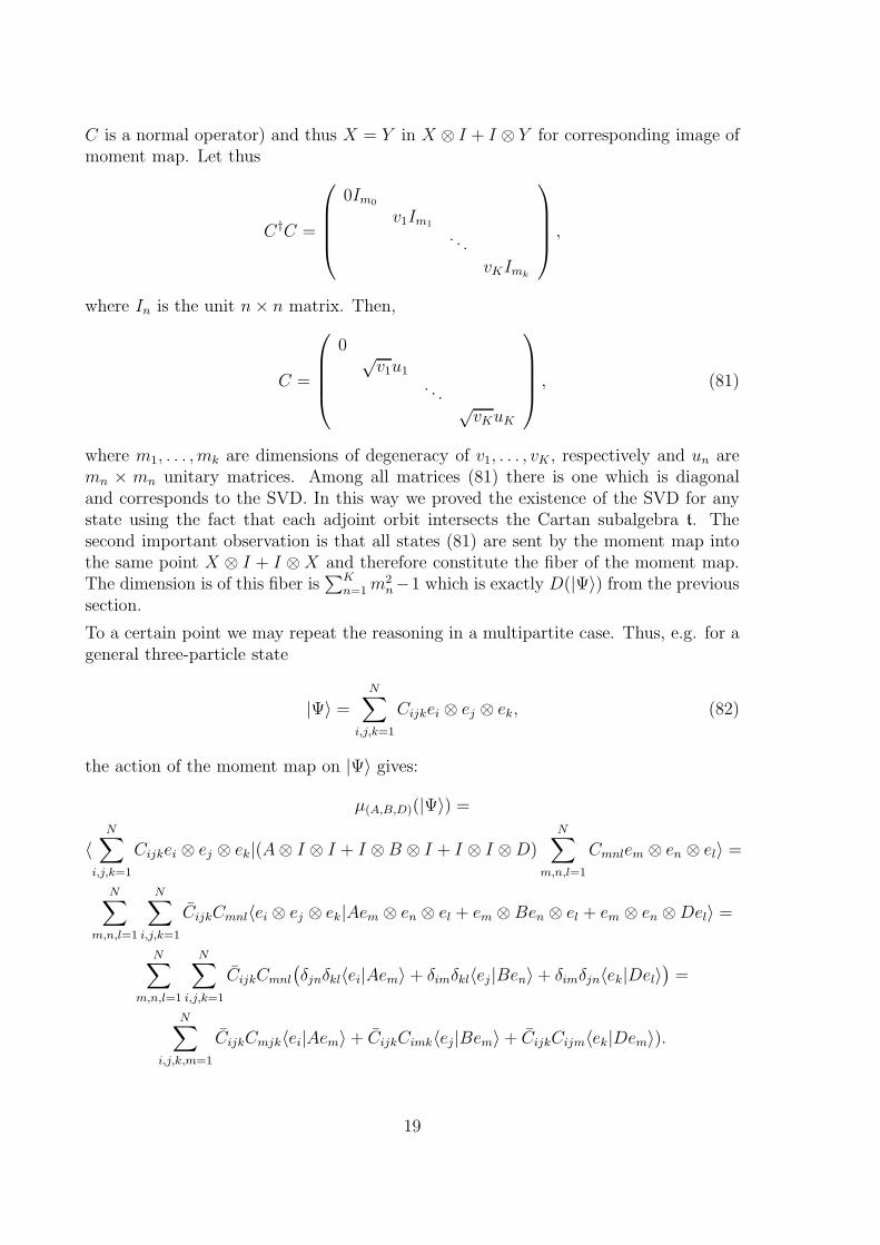
C is a normal operator) and thus X = Y in X ⊗ I + I ⊗ Y for corresponding image ofmoment map. Let thus

C†C =

0Im0

v1Im1

. . .

vKImk

,

where In is the unit n× n matrix. Then,

C =

0 √v1u1

. . . √vKuK

, (81)

where m1, . . . , mk are dimensions of degeneracy of v1, . . . , vK , respectively and un aremn × mn unitary matrices. Among all matrices (81) there is one which is diagonaland corresponds to the SVD. In this way we proved the existence of the SVD for anystate using the fact that each adjoint orbit intersects the Cartan subalgebra t. Thesecond important observation is that all states (81) are sent by the moment map intothe same point X ⊗ I + I ⊗X and therefore constitute the fiber of the moment map.The dimension is of this fiber is

∑Kn=1m

2n−1 which is exactly D(|Ψ〉) from the previous

section.

To a certain point we may repeat the reasoning in a multipartite case. Thus, e.g. for ageneral three-particle state

|Ψ〉 =

N∑

i,j,k=1

Cijkei ⊗ ej ⊗ ek, (82)

the action of the moment map on |Ψ〉 gives:

µ(A,B,D)(|Ψ〉) =

〈N∑

i,j,k=1

Cijkei ⊗ ej ⊗ ek|(A⊗ I ⊗ I + I ⊗B ⊗ I + I ⊗ I ⊗D)N∑

m,n,l=1

Cmnlem ⊗ en ⊗ el〉 =

N∑

m,n,l=1

N∑

i,j,k=1

CijkCmnl〈ei ⊗ ej ⊗ ek|Aem ⊗ en ⊗ el + em ⊗ Ben ⊗ el + em ⊗ en ⊗Del〉 =

N∑

m,n,l=1

N∑

i,j,k=1

CijkCmnl

(

δjnδkl〈ei|Aem〉 + δimδkl〈ej |Ben〉 + δimδjn〈ek|Del〉)

=

N∑

i,j,k,m=1

CijkCmjk〈ei|Aem〉 + CijkCimk〈ej|Bem〉 + CijkCijm〈ek|Dem〉).

19

Again, we want to find conditions for Cijk under which µ(A,B,D)(|Ψ〉) belongs to t∗.Substituting for A, B, and D basis elements from k− t and again using (80) we get:

N∑

j,k=1

CnjkCljk +

N∑

j,k=1

CljkCnjk = 0,

N∑

j,k=1

CnjkCljk −N∑

j,k=1

CljkCnjk = 0,

and similar two pairs of equations for other combination of indices. If we now define

(C1)nl =N∑

j,k=1

CnjkCljk,

(C2)nl =

N∑

j,k=1

CjnkCjlk, (83)

(C3)nl =N∑

j,k=1

CjknCjkl,

the obtained conditions mean that the matrices C1, C2, C3 are diagonal. In this case itis not generally true that C1 = C2 = C3 so the corresponding state in t is X ⊗ I ⊗ I +I ⊗ Y ⊗ I + I ⊗ I ⊗ Z where X 6= Y 6= Z.

Up to now we know that any state |Ψ〉 =∑N

i,j,k=1 Cijkei ⊗ ej ⊗ ek can be taken by local

unitary transformation U1 ⊗ U2 ⊗ U3 to the state |Ψ〉 =∑N

i,j,k=1Cijkei ⊗ ej ⊗ ek wherethe coefficients Cijk fulfill (83). This statement has a deeper physical meaning. Thediagonal elements of C1, C2, C3 constitute probabilities to obtain basis vectors {ei} insome local measurements performed on state |Ψ〉. The conditions (83) say that any statecan be transformed by local unitary transformation to the state which is determinedby these local measurements. It is natural to ask now how to find such a unitary localtransformation.

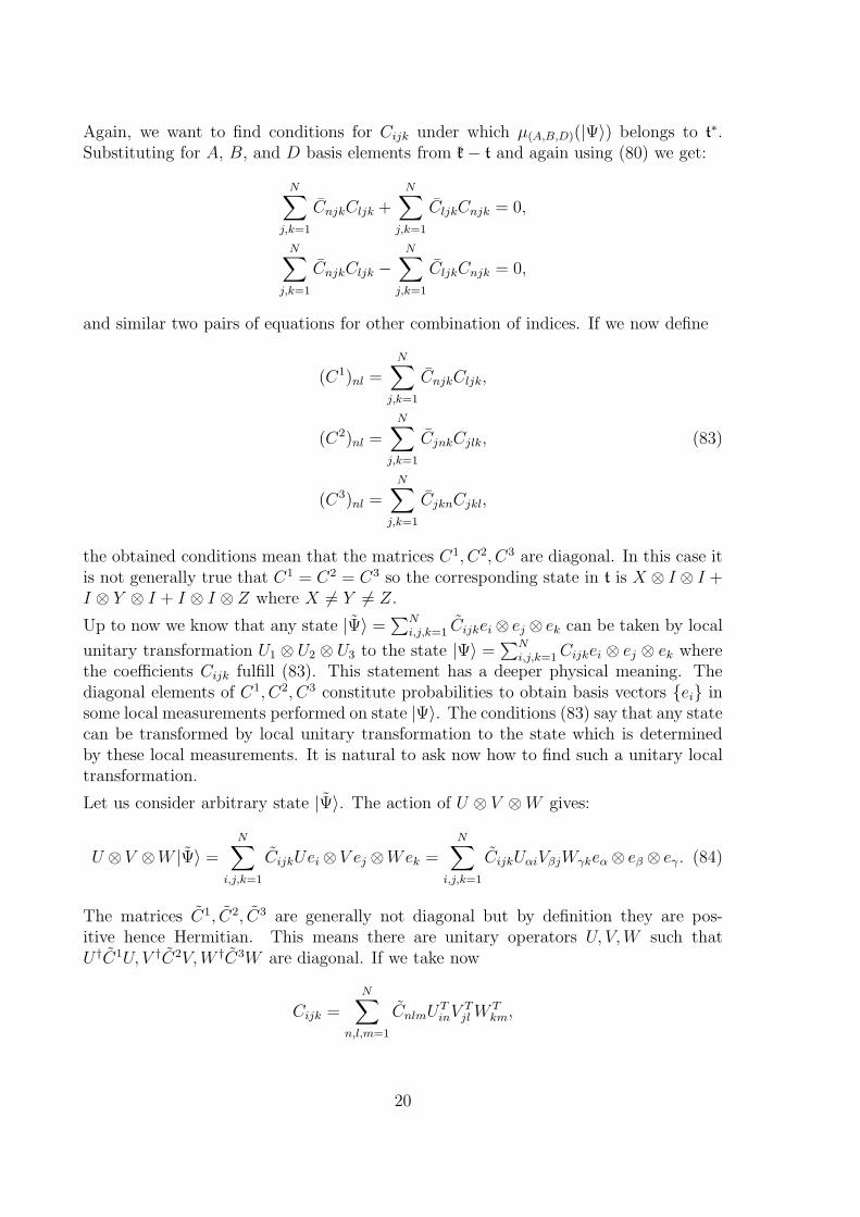
Let us consider arbitrary state |Ψ〉. The action of U ⊗ V ⊗W gives:

U ⊗ V ⊗W |Ψ〉 =N∑

i,j,k=1

CijkUei ⊗ V ej ⊗Wek =N∑

i,j,k=1

CijkUαiVβjWγkeα ⊗ eβ ⊗ eγ . (84)

The matrices C1, C2, C3 are generally not diagonal but by definition they are pos-itive hence Hermitian. This means there are unitary operators U, V,W such thatU †C1U, V †C2V,W †C3W are diagonal. If we take now

Cijk =

N∑

n,l,m=1

CnlmUTinV

Tjl W

Tkm,

20

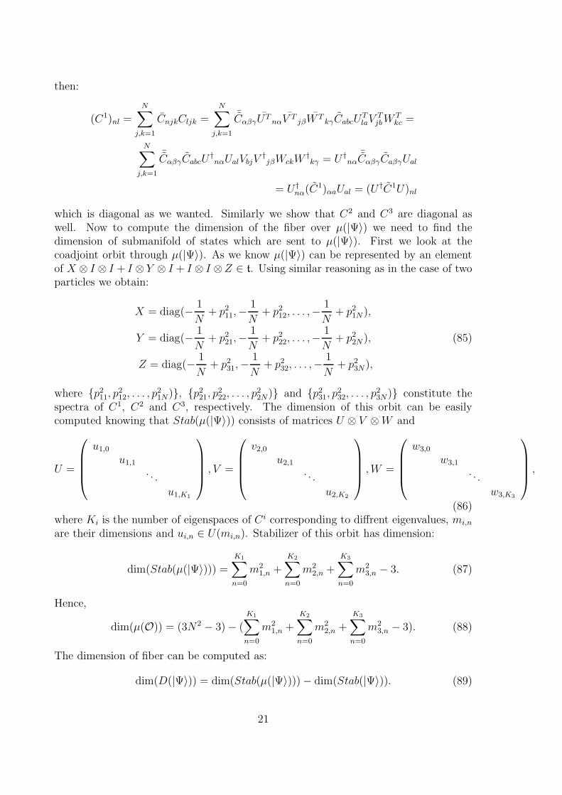
then:

(C1)nl =

N∑

j,k=1

CnjkCljk =

N∑

j,k=1

¯CαβγUTnαV T

jβW TkγCabcU

TlaV

TjbW

Tkc =

N∑

j,k=1

¯CαβγCabcU†nαUalVbjV

†jβWckW

†kγ = U †

nα¯CαβγCaβγUal

= U †nα(C1)αaUal = (U †C1U)nl

which is diagonal as we wanted. Similarly we show that C2 and C3 are diagonal aswell. Now to compute the dimension of the fiber over µ(|Ψ〉) we need to find thedimension of submanifold of states which are sent to µ(|Ψ〉). First we look at thecoadjoint orbit through µ(|Ψ〉). As we know µ(|Ψ〉) can be represented by an elementof X ⊗ I ⊗ I + I ⊗ Y ⊗ I + I ⊗ I ⊗Z ∈ t. Using similar reasoning as in the case of twoparticles we obtain:

X = diag(− 1

N+ p211,−

1

N+ p212, . . . ,−

1

N+ p21N ),

Y = diag(− 1

N+ p221,−

1

N+ p222, . . . ,−

1

N+ p22N ), (85)

Z = diag(− 1

N+ p231,−

1

N+ p232, . . . ,−

1

N+ p23N),

where {p211, p212, . . . , p21N)}, {p221, p222, . . . , p22N)} and {p231, p232, . . . , p23N)} constitute thespectra of C1, C2 and C3, respectively. The dimension of this orbit can be easilycomputed knowing that Stab(µ(|Ψ〉)) consists of matrices U ⊗ V ⊗W and

U =

u1,0

u1,1

. . .

u1,K1

, V =

v2,0u2,1

. . .

u2,K2

,W =

w3,0

w3,1

. . .

w3,K3

,

(86)where Ki is the number of eigenspaces of C i corresponding to diffrent eigenvalues, mi,n

are their dimensions and ui,n ∈ U(mi,n). Stabilizer of this orbit has dimension:

dim(Stab(µ(|Ψ〉))) =

K1∑

n=0

m21,n +

K2∑

n=0

m22,n +

K3∑

n=0

m23,n − 3. (87)

Hence,

dim(µ(O)) = (3N2 − 3) − (

K1∑

n=0

m21,n +

K2∑

n=0

m22,n +

K3∑

n=0

m23,n − 3). (88)

The dimension of fiber can be computed as:

dim(D(|Ψ〉)) = dim(Stab(µ(|Ψ〉))) − dim(Stab(|Ψ〉)). (89)

21

Notice that if C1, C2, C3 have nontrivial kernels then in decomposition of Ψ thereare no elements ei ⊗ ej ⊗ ek where ei ∈ Ker(C1) or ej ∈ Ker(C2) or ej ∈ Ker(C3).This means that acting on |Ψ〉 by unitary operators from Stab(µ(|Ψ〉)) which can berestricted to the kernels of C1, C2, C3 we do not change the state |Ψ〉. We find thus anupper bound for the dimension of the degeneracy space as

K1∑

n=1

m21,n +

K2∑

n=1

m22,n +

K3∑

n=1

m23,n − 3. (90)

The dimension of a fiber is at least

max{K1∑

n=1

m21,n,

K2∑

n=1

m22,n,

K3∑

n=1

m23,n} − 1. (91)

Indeed, the conditions (83) allow us to write the state |Ψ〉 as

|Ψ〉 =

N∑

i

p1iei ⊗ vi, (92)

where

vi =∑

jk

1

p1iCijkej ⊗ ek, i = 1, . . . , N (93)

constitute a set of orthonormal vectors. We can treat (92) as a bipartite decompositionof Ψ in the orthonormal bases {ei} and {vi}. In these bases Ψ is thus represented bythe matrix C,

C =

0Im10

p1Im1,1

. . .

pK1Im1,K1

,

where pi are different eigenvalues p1i. Application of U ⊗ I ⊗ I ∈ Stab(µ(|Ψ〉)) yields:

C ′ =

0u10

p1u11

. . .

pK1u1,K1

, (94)

Clearly, the matrices C ′ of the above form constitute a manifold of dimension∑K1

n=1m21,n−

1. In the case of two particles this is the whole fiber because acting with U⊗I and I⊗Vwe get exactly the same manifold. For multipartite systems, like the three particle casewe consider, we have to take into account that acting with I ⊗ V ⊗ I and I ⊗ I ⊗Wmay produce manifolds of larger dimensionalities which leads thus to the estimate (91).Summing up we have

max{K1∑

n=1

m21,n,

K2∑

n=1

m22,n,

K3∑

n=1

m23,n} − 1 ≤ D(|Ψ〉) ≤

K1∑

n=1

m21,n +

K2∑

n=1

m22,n +

K3∑

n=1

m23,n − 3.

(95)

22

Thus an orbit is symplectic if and only if

K1∑

n=1

m21,n = 1,

K2∑

n=1

m22,n = 1,

K3∑

n=1

m23,n = 1.

But this means that the state |Ψ〉 is separable because it reduces to one of the statesei⊗ej⊗ek. If the state is separable than of course by local operations we can transformit to the state e1 ⊗ e1 ⊗ e1 and then (96) is fulfilled. In this way we found an easyway to check if a state is separable and showed that it is equivalent to the fact thatassociated orbit is symplectic. We also have an estimate for dimensions of degeneracyspaces for entangled states. A generalization to cases of more than three particles isstraightforward. So we have following

Theorem 5 In the case of M identical but distinguishable particles there is only onesymplectic orbit in the projective space P(

⊗M

n=1CN). This orbit contains all separable

states and is Kahler. Orbits through entangled states are not symplectic.

Knowing this and making use of Corollary 1 we arrive with

Fact 7 In the case of M identical but distinguishable particles the dimension od degen-eracy space D(|Ψ〉) gives well defined entanglement measure. Fora any state |Ψ〉 theestimate for this measure is given by formula analogous to (95).

10 Indistinguishable particles

The Kostant-Sternberg theorem can be directly applied also to indistinguishable par-ticles, i.e. bosons and fermions. For M bosons the relevant group is K = SU(N)represented in V = SymM

(

CN)

. As above we want to check which orbits of K-actionare symplectic in the projective space P(V ). The best way to understand the problem isto do some nontrivial example and then generalize the obtained result. To this end letus consider the simplest case of M = 2 and N = 3, i.e. the representation of SU(3) inSym2 (C3). First we notice that the representation of SU(N) in Sym2

(

CN)

is irreducible[18]. From the Kostant-Sternberg theorem it follows that it is enough to investigatestructure of the sl(3,C) representation on Sym2

(

CN)

. The g = sl(3,C) algebra iseight-dimensional and can be decomposed as g = n− ⊕ h ⊕ n+, where h is the Car-tan subalgebra consisting of traceless diagonal matrixes and n+ = Span(E12, E13, E23),n− = Span(E21, E31, E32). We define three linear functionals Li : h → C,

Li(diag(a1, a2, a3)) = ai, i ∈ {1, 2, 3} (96)

Let us choose a basis B in Sym2 (C3), B = {e1⊗e1, e2⊗e2, e3⊗e3, e1⊗e2+e2⊗e1, e1⊗e3+e3⊗e1, e2⊗e3+e3⊗e2} where ei ∈ C3 are the standard basis vectors. The action ofthe Lie algebra g on Sym2 (C3) is a usual action of the tensor product of representations.Construction of the representation of sl(3,C) on Sym2 (C3) is straightforward, we take

23

the vector e1⊗ e1 which is the highest weight vector (it is an eigenvector of all elementsin h and it is annihilated by n+ ), and we act on it with operators from n−. As a resultwe obtain a decomposition of V = Sym2 (C3) into the direct sum V =

⊕

Vλ where theone-dimensional weight spaces Vλ are spanned by the basis vectors of B. The weightsλ ∈ h∗ can be now calculated as 1

H(ei ⊗ ei) = 2Li(H)ei ⊗ ei i = 1, 2, 3,

H(ei ⊗ ej + ej ⊗ ei) = (Li + Lj)(H) (ei ⊗ ej + ej ⊗ ei) (97)

We know that only orbits passing through weight vectors might be symplectic. We havethe following sl(2,C) triples in sl(3,C): (Eij , Eji, Hij = [Eij , Eji]). The orbit througha weight vector v with a weight λ is symplectic if and only if for every operator fromn+ the following implication is true: λ(Hij) = 0 ⇒ Eij(v) = 0 = Eji(v). There are twocases to consider,

• Vectors of the form ei ⊗ ei, i = 1, 2, 3. The weight of the ei ⊗ ei state is 2Li

so 2Li(Hkj) = 0 only when k 6= i and j 6= i. In this case Ekj(ei ⊗ ei) = 0because to give nonzero result matrix Ekj must have one in the i-th column. Thecorresponding orbit is thus symplectic. Obviously, all these vectors lie on theorbit through the highest weight vector e1 ⊗ e1

• Vectors of the form ei⊗ej +ej⊗ei where i 6= j.The weight of this vector is Li+Lj

so (Li +Lj)(Hkl) = 0 only if k = i and j = l. In this case Eij(ei⊗ej +ej ⊗ei) 6= 0because Eijej 6= 0. In conclusion the orbit through ei⊗ej+ej⊗ei is not symplectic.

Let us now return to the problem mentioned in Section 2.2. If we define nonentangledbosonic states as antisymmetrizations of simple tensors (or, more precisely, as corre-sponding points in the projective space) then we clearly have two, inequivalent from thegeometric point of view, types of nonentanglement. Non-entangled states of two differ-ent types are not connected by local unitary transformations which is in contrast to thefamiliar situation of distinguishable particles and intuitions build upon the fact that allseparable states of distinguishable particles can be obtained from a single one by localtransformations. Although this is obviously acceptable, it remains an open problemwhat is a physical meaning of two different types of nonentanglement. If, instead, weadopt the second definition identifying nonentangled bosonic states as points in theprojective space corresponding to tensor products of the same vector we encounter thesame situation as in the case of distinguishable particles - the nonentangled states forma unique symplectic orbit, and the degeneracy of the symplectic form can be used as ameasure of entanglement for entangled states.

The case of fermions does not lead to any ambiguities of the above type. Calculationssimilar to those made for bosons lead to a conclusion that nonentangled states formthe unique symplectic orbit. Indeed, let us consider as an example K = SU(N) andV =

∧2C

N corresponding to two fermions of spin (N − 1)/2 with the single-particle

1Remember that we represent k in the symmetric tensor product, hence H(ei⊗ ei) has the meaningof (H ⊗ I + I ⊗H)(ei ⊗ ei) = Hei ⊗ ei + ei ⊗Hei etc.

24

space H1 = CN . In terms of the previously introduced standard bases ei and Eij

adapted to N dimensions V is spanned by ekl = ek ⊗ el − el ⊗ ek, with k < l the highestweight vector is e12 and

Eij ekl = δjleki + δjkeil (98)

where we denote ekl = −elk for k > l. Acting by Eij with i > j on e12 we obtainremaining weight vectors, which according to (98) are all of the form ekl (in fact withl = 1 or 2), with weights Li + Lj (we extended in an obvious way the definition (96)to N dimensions). As remarked (Li + Lj)(Hkl) = 0 implies k = i, j = l but thenEijekl = 0 = Ejiekl.

11 Summary and outlook

We presented an geometric description of the set of pure states of composite quantumsystems in terms of natural symplectic structure in the space of states. Nonentangledstates form a unique symplectic orbit through the highest weight vector of the appro-priate representation of the group of local transformations whereas entangled statesare characterized by the degeneracy of the symplectic form. The degeneracy can bethus used as a kind of geometric measure of entanglement. We were able to calculatethe degeneracy in many relevant cases and give some estimates for the most generalsystem of arbitrary number of constituents with an arbitrary dimension of the singleparticle space. Let us remark that there exists a useful characterization of the high-est weight vector orbits which allows to generalize and estimate effectively some otherentanglement measures [19].

An obvious question is whether a method can be adapted to the case of mixed states.This problem, as well as applications of the obtained results to identifying, so called,locally unitary equivalent multiparticle states [20] and finding ”canonical” forms ofthem we postpone to forthcoming publications.

12 Acknowledgments

The support by SFB/TR12 Symmetries and Universality in Mesoscopic Systems pro-gram of the Deutsche Forschungsgemeischaft and Polish MNiSW grant no. DFG-SFB/38/2007 is gratefully acknowledged.

25

13 Appendix

13.1 Symplectic structure on coadjoint orbits

Let K be a semisimple compact Lie group, k its Lie algebra, and k∗ the dual space tok. The coadjoint action of K on k∗ is given by

Ad∗g : k∗ → k∗ (99)

〈Ad∗gα, Y 〉 = 〈α,Adg−1Y 〉 = 〈α, g−1Y g〉, g ∈ K, Y ∈ k, α ∈ k∗,

where Ad is the adjoint action of K. It can be easily checked that (99) is well defined.The coadjoint orbit Oα passing through α ∈ k∗ is the orbit of the coadjoint action of Kon α

Oα = {Ad∗gα : g ∈ K} (100)

Our goal now is to define a K-invariant symplectic form ω on Oα. Such a form acts ontangent vectors so it is reasonable to first look at their structure. Since k∗ is a vectorspace its tangent space at any point is again k∗. For any X ∈ k let X ∈ TαOα be avector tangent to the curve t 7→ Ad∗

exp(tX)α. We have then,

〈X, Y 〉 = 〈 ddt

∣

∣

∣

∣

t=0

Ad∗exp(tX)α, Y 〉 =

d

dt

∣

∣

∣

∣

t=0

〈α,Adexp(−tX)Y 〉 = 〈α, [Y,X ]〉, (101)

where Y ∈ k. Thus X is an element of k∗ given by

X = 〈α, [ · , X ]〉. (102)

It is now interesting to ask how this tangent vector transform when pushed by anelement g ∈ K, i.e. to consider the vector gX ∈ TAd∗

gαOα tangent to the curve t 7→

Ad∗gAd∗

exp(tX)α. We have

〈gX, Y 〉 = 〈 ddt

∣

∣

∣

∣

t=0

Ad∗gAd∗

exp(tX)α, Y 〉 =d

dt

∣

∣

∣

∣

t=0

〈α,Adexp(−tX)Adg−1Y 〉 = (103)

= 〈α, [Adg−1Y,X ]〉 = 〈α, [Adg−1Y,Adg−1AdgX ] =

= 〈α,Adg−1 [Y,AdgX ]〉 = 〈Ad∗gα, [Y,AdgX ]〉.

Hence gX is an element of k∗ given by

gX = 〈Ad∗gα, [ · ,AdgX ]〉. (104)

We may now define our symplectic form at any β ∈ Oα as

ωβ(X, Y ) = 〈β, [X, Y ]〉. (105)

The form is non-degenerate on Oα because

∀Y ∈ k 〈β, [X, Y ]〉 = 0 ⇔ ∀Y ∈ k 〈X, Y 〉 = 0 ⇔ X = 0. (106)

26

It is also K-invariant because

ωAd∗gβ(gX, gY ) = 〈Ad∗gβ, [AdgX,AdgY ]〉 = 〈β,Adg−1Adg[X, Y ]〉 = (107)

= 〈β, [X, Y ]〉 = ωβ(X, Y ).

Thus we need only to check if ω is closed. But we know that for any differential 2-formthe following is true

dω(X, Y , Z) = Xω(Y , Z) + Y ω(Z, X) + Zω(X, Y )+ (108)

−(ω([X, Y ], Z) + ω([Y , Z], X) + ω([Z, X], Y )).

Taking X = 〈Ad∗gβ, [ · , Ad(g)X ]〉 and similarly for Y and Z we see that that first three

terms in (108) vanish because ω is K-invariant. The sum of next three terms is alsozero due to the Jacobi identity. This way we arrive at a well defined symplectic formon Oα.

13.2 Kahler structure

Let us start with definition of Kahler manifold.

Definition 2 Let M be a complex manifold dimCM = n and let ω be a symplectic formon M treated as 2n-dimensional real manifold. Then M is called a Kahler manifold ifat every p ∈ X the complex structure i on TpX (multiplication by imaginary unit) andthe antisymmetric form ωp has the following property:

ωp(iv, iw) = ω(v, w), (109)

that is i ∈ Sp(TpM) (the symplectic group of TpM).

Assume M is a Kahler manifold. Then we can define a symmetric nondegenerate formb on M

b(v, w) = ω(v, iw). (110)

Indeed we have

b(v, w) = ω(v, iw) = ω(iv, i2w) = −ω(iv, w) = ω(w, iv) = b(w, v). (111)

The form b is non-degenerate because

∀w ∈ TpM b(v, w) = 0 ⇔ ∀w ∈ TpM ω(w, iv) = 0 ⇔ v = 0. (112)

It is also i-invariant

b(iv, iw) = ω(iv, i2w) = ω(v, iw) = b(v, w). (113)

We have now the following definition.

27

Definition 3 A Kahler structure on M is called positive if and only if the correspondingsymmetric form b is positive.

It is straightforward to check that having such an i-invariant non-degenerate symmet-ric form b on M we can a define non-degenerate i-invariant antisymmetric 2-form byω(v, w) = b(iv, w). We will need only one more theorem (see [12] for a detailed proof).

Theorem 6 Let M be a positive Kahler manifold. Then any complex submanifoldN ⊂ M is also a Kahler manifold.

The assumption that M is a positive Kahler manifold (not just a Kahler manifold)is very important due to the fact that restriction of the symmetric form b to N isthen non-degenerate and i-invariant. Now using b|N we can define a non-degeneratei-invariant antisymmetric 2-form on N which is a restriction of ω defined on the wholeM , and hence is symplectic.

13.2.1 Kahler structure on P(V )

Consider a complex vector space V , dimCV = n with a Hermitian scalar product (·|·).The complex projective space P(V ) of V is defined

P(V ) = V/ ∼, (114)

where the equivalence ∼ is defined by

v ∼ w ⇔ w = αv α ∈ C∗, (115)

where C∗ = C \ {0}. The standard way to realize P(V ) is by two steps

Va−→ S(V )

b−→ P(V ), (116)

where the step a is a quotient by the dilation v ∼ αv for a ∈ R∗ and the step b is

a quotient by the rotations v ∼ eiφv. The result of the quotient a is the real sphereS(V ) = {v ∈ v : ‖v‖ = 1}. The quotient b gives S(V )/S1 = S2n−1/S1, where S1

represents the group of rotations. It is well known fact that the complex projectivespace P(V ) is a complex manifold and dimCP(V ) = n − 1. Let π : V \ {0} → P(V )be the projection defined by equivalence ∼. The tangent space to P(V ) at z = π(v) isTzP(V ) = πv(TvV ). It is good question to ask what is πv(ξ), where ξ ∈ TvV . Considerthe curve t 7→ v(t) ∈ V , v(0) = v. Then

ξ =d

dt

∣

∣

∣

∣

t=0

v(t). (117)

We first apply the map a to v(t). As a result we get a curve t 7→ v(t)‖v(t)‖

∈ S(V ). Applying

the map b amounts to getting rid of the rotation eiφv, hence finally the curve in P(v) isgiven as

t 7→ v(t)

‖v(t)‖ − v( v

‖v‖∣

∣

v(t)

‖v(t)‖)

. (118)

28

The tangent vector to this curve is thus

d

dt

∣

∣

∣

∣

t=0

v(t)

‖v(t)‖ − d

dt

∣

∣

∣

∣

t=0

v( v

‖v‖∣

∣

v(t)

‖v(t)‖)

=ξ

‖v‖ − v

‖v‖( v

‖v‖∣

∣

ξ

‖v‖)

. (119)

Hence for any vector ξ ∈ TvV we obtain the corresponding vector πv(ξ) ∈ Tπ(v)P(V ) as

the orthogonal complement of ξ

‖v‖to the subspace Cv in the Hermitian scalar product

(·|·). Let us introduce a Hermitian scalar product on P(v) by

h(πv(ξ), πv(η)) =

(

1

‖v‖ξ(v|v) − (v|ξ)v

(v|v)

∣

∣

∣

∣

1

‖v‖η(v|v) − (v|η)v

(v|v)

)

, (120)

which, after some calculations, reduces to

h(πv(ξ), πv(η)) =(ξ|η)(v|v) − (ξ|v)(v|η)

(v|v)2. (121)

Of course, h is a well defined, that is non-degenerate, positive Hermitian form on PV .Indeed, for any z = π(v) we have TzP(V ) = (Cv)⊥. Knowing this we can introduce anon-degenerate antisymmetric 2-form ω on P(V ) as the imaginary part of h(·, ·)

ω(πv(ξ), πv(η)) = −Imh(πv(ξ), πv(η)). (122)

It is straightforward to check that ω is not only i-invariant but also U(V )-invariant. Tocheck that it is also closed notice that U(V ) is acting transitively on V which meansthe vectors Av, where A ∈ u(V ) span TvV . Hence,

ω(πv(Av), πv(Bv)) = −Im(Av|Bv)(v|v) − (Av|v)(v|Bv)

(v|v)2, A, B ∈ u(V ). (123)

But (Av|v)(v|Bv) is real since (Av|v) and (v|Bv) are imaginary (this is because A† =−A for all A ∈ u(V )). Hence,

ω(πv(Av), πv(Bv)) = −Im(Av|Bv)

(v|v)=

i([A,B]v|v)

2(v|v), A, B ∈ u(V ). (124)

Now making use of Equation (108) for vector fields πUv(UAU∗Uv) and similarly forB and C we find, by the same argument as for coadjoint orbits, that dω = 0. Thismeans P(V ) is a Kahler manifold. It is also a positive Kahler manifold because thecorresponding symmetric form b given by

b(πv(ξ), πv(η)) = −Reh(πv(ξ), πv(η)), (125)

is clearly positive.

References

[1] Horodecki, R., Horodecki, P., Horodecki, M., and Horodecki, K.: Quantum entan-glement. Rev. Mod. Phys. 81, 865–942 (2009)

29

[2] Werner, R.: Quantum states with Einstein-Podolsky-Rosen correlation admittinga hidden-variable model. Phys. Rev. A 40, 4277–4281 (1989)

[3] Schliemann, J., Cirac J.I., Kus, M., Lewenstein M., and Loss, D.: Quantumcorrelations in two-fermion systems. Phys. Rev. A 64, 022303 (2001)

[4] Eckert K., Schliemann, J. Bruß, D., and Lewenstein, M.: Quantum correlations insystems of identical particles. Ann. Phys. 299, 88–127 (2002)

[5] Ghirardi, G., Marinatto, L., and Weber, T.: Entanglement and properties ofcomposite quantum systems, a conceptual and mathematical analysis. J. Stat.Phys. 108, 49–122 (2002)

[6] Li, Y.S. Zeng, B., Liu, X.S., and Long, G.L.: Entanglement in a two-identical-particle system. Phys. Rev. A 64, 054302 (2001)

[7] Paskauskas, R. and You, L.: Quantum correlations in two-boson wave functions.Phys. Rev. A 64, 042310 (2001)

[8] Klyachko, A.: Dynamic symmetry approach to entanglement. Preprint arXiv0802.4008, 2008.

[9] Bengtsson, I.: A curious geometrical fact about entanglement. Preprint arXiv0707.3512, 2007.

[10] Kus, M. and I.Bengtsson.: “Classical” quantum states. Phys. Rev. A 80, 022319(2009)

[11] Kostant, B. and Sternberg, B.: Symplectic projective orbits. New directions inapplied mathematics, papers presented April 25/26, 1980, on the occasion of theCase Centennial Celebration (Hilton, P. J. and Young, G. S., eds.) New York:Springer, 1982, pp 81–84

[12] Guillemin, V. and Sternberg S.: Symplectic techniques in physics. Cambridge:Cambridge University Press, 1984

[13] Perelomov, A.: Generalized coherent states and their applications. Springer: Hei-delberg, 1986

[14] Hall, B. C.: Lie groups, Lie algebras, and representations, an elementary intro-duction. New York: Springer, 2003

[15] Kirillov, A. A.: Lectures on the orbit method. Graduate Studies in Mathematicsvol. 64. Providence: American Mathematical Society, 2004

[16] Horn, R. A. and Johnson, C. R.: Matrix analysis. Cambridge: Cambridge Univer-sity Press, 1985

[17] Sino lecka, M. M., Zyczkowski, K., and Kus, M.: Manifolds of equal entanglementfor composite quantum system. Acta Phys. Pol. 33, 2081–2095 (2002)

30

[18] Fulton, W. and Harris, J.: Representation theory. A first course. New York:Springer, 1991

[19] Kotowski, M., Kotowski, M., and Kus M.: Universal nonlinear entanglementwitnesses. Phys. Rev. A 81 062318 (2010)

[20] B.Kraus. Local unitary equivalence of multipartite pure states. Phys. Rev. Lett.104 020504 (2010).

31