ANNALES DE LA FACULTÉ DES SCIENCES DE TOULOUSE

OLE E. BARNDORFF-NIELSEN

PETER E. JUPPStatistics, yokes and symplectic geometryAnnales de la faculté des sciences de Toulouse 6e série, tome 6, no 3(1997), p. 389-427<http://www.numdam.org/item?id=AFST_1997_6_6_3_389_0>

© Université Paul Sabatier, 1997, tous droits réservés.

L’accès aux archives de la revue « Annales de la faculté des sciences deToulouse » (http://picard.ups-tlse.fr/~annales/) implique l’accord avec lesconditions générales d’utilisation (http://www.numdam.org/conditions).Toute utilisation commerciale ou impression systématique est constitu-tive d’une infraction pénale. Toute copie ou impression de ce fichierdoit contenir la présente mention de copyright.

Article numérisé dans le cadre du programmeNumérisation de documents anciens mathématiques

http://www.numdam.org/

- 389 -

Statistics, Yokes and Symplectic Geometry(*)

OLE E. BARNDORFF-NIELSEN(1)and

PETER E. JUPP(2)

Annales de la Faculté des Sciences de Toulouse Vol. VI, n° 3, 1997

RÉSUMÉ. - Nous établissons et étudions un lien entre jougs et formessymplectiques. Nous montrons que les jougs normalises correspondenta certaines formes symplectiques. Nous présentons une méthode pourconstruire de nouveaux jougs à partir de jougs donnés. Celle-ci est

motivée en partie par la dualite entre la formulation hamiltonienne etla formulation lagrangienne de la mécanique conservative. Nous nous

proposons quelques variantes de cette construction.

MOTS-CLfS : Application moment, hamiltonien, joug de vraisemblanceesperee, joug de vraisemblance observée, lagrangien, sous-variété lagran-gienne, tenseurs.

ABSTRACT. - A relationship between yokes and symplectic forms isestablished and explored. It is shown that normalised yokes correspondto certain symplectic forms. A method of obtaining new yokes from oldis given, motivated partly by the duality between the Hamiltonian andLagrangian formulations of conservative mechanics. Some variants of thisconstruction are suggested.

KEY-WORDS : expected likelihood yoke, Hamiltonian, Lagrangian sub-manifold, momentum map, observed likelihood yoke, tensors.

AMS Classiflcation : 58F05, 62E20

(*) Reçu le 10 juillet 1995(1) Department of Mathematical Sciences, Aarhus University, Ny Munkegade, DK-

8000 Aarhus C (Denmark)(2) School of Mathematical and Computational Sciences, University of St Andrews,

North Haugh, St Andrews KY16 9SS (United Kingdom)

1. Introduction

In the differential-geometric approach to statistical asymptotics a central

concept is that of a yoke, key examples being the observed and expectedlikelihood yokes.A yoke on a manifold M is a real-valued function on the "square" M x M

of M, satisfying conditions (2.1) and (2.2) below (Barndorff-Nielsen [7]).Yokes which are restricted to be non-negative and are zero only on the

diagonal are known as contrast functions. For uses of contrast functions instatistics see, e.g., Eguchi [16] and Skovgaard [24]. In applications of yokesto statistical asymptotics we are particularly interested in the values of the

yoke near the diagonal 0~ of M x M, ( c~ A suitable neighbourhood of Aj~ in M x M can be regarded as the total

space of the normal bundle of 0~ in M x M and this normal bundle is

isomorphic to the tangent bundle TM of M. Furthermore, a yoke on Mdetermines a (possibly indefinite) Riemannian metric, which can be used toidentify the tangent bundle TM with the cotangent bundle T*M. .

One of the main contexts in which cotangent bundles occur is in conser-vative mechanics (see e.g., Abraham and Marsden [I], and Marsden [19]),where they are known as the phase spaces. The geometrical concept is

that of a symplectic structure. A survey of symplectic geometry and its

applications is given by Arnol’d and Givental’ [3].The role of Hamiltonians in conservative mechanics and their relation to

exponential families suggest that symplectic geometry may have a naturalrole to play in statistics. It is relevant here also to mention the work

of Combet [13] which discusses certain connections between symplecticgeometry and Laplace’s method for exponential integrals.

In view of the results to be described below we think it fair to say that

there exists a natural link, via the concept of yokes, between statisticsand symplectic geometry. How useful this link may be seems difficult toassess at present. Other links have been discussed by T. Friedrich andY. Nakamura. Friedrich [17] established some connections between expected(Fisher) information and symplectic structures. However, as indicated

in Remark 3.4, his approach and results are quite different from thoseconsidered here. Nakamura ([22], [23]) has shown that certain parametricstatistical models in which the parameter space M is an even-dimensionalvector space (and so has the symplectic structure of the cotangent space of

a vector space) give rise to completely integrable Hamiltonian systems onM. In contrast to these, the Hamiltonian systems considered here arise inthe more general context of yokes on arbitrary manifolds M and are definedon some neighbourhood of 0~ in M x M.

Section 2 reviews the necessary background on yokes, symplectic struc-tures and mechanics. In Section 3, we show that every yoke on a manifoldM gives rise to a symplectic form, at least on some neighbourhood of thediagonal of M x M, and in some important cases on all of M x M. Bypassing to germs, i.e., by identifying yokes or symplectic forms which agreein some neighbourhood of the diagonal, we show that normalised yokes arealmost equivalent to symplectic forms of a certain type. (However, fromthe local viewpoint there is nothing special about those symplectic formswhich are given by yokes, since Darboux’s Theorem shows that locally ev-ery symplectic form can be obtained from some yoke; see Example 3.1.) InSection 4, we consider some uses of the symplectic form given by a yoke.

There is an analogy between conservative mechanics and the geometryof yokes in that symplectic forms play an important part in both areas. InSection 5, this analogy is used to transfer the duality between the Hamilto-nian and Lagrangian versions of conservative mechanics to a constructionfor obtaining from any normalised yoke g another yoke g, called the La-grangian of g, which has the same metric as g and is, in some sense, closeto the dual yoke g* of g.

Section 6 considers Lie group actions on the manifold and the associatedmomentum map, which takes values in the dual of the appropriate Liealgebra.

An outline version of some of the material presented in this paper is givenin Barndorff-Nielsen and Jupp [11]. .

2. Preliminaries

2.1 Yokes

Let M be a smooth manifold. We shall sometimes use local coordinates

(cv 1, ... , wd) on M and, correspondingly, local coordinates ... , wd; ;w’ l , ..., on M x M. Furthermore, we use the notations

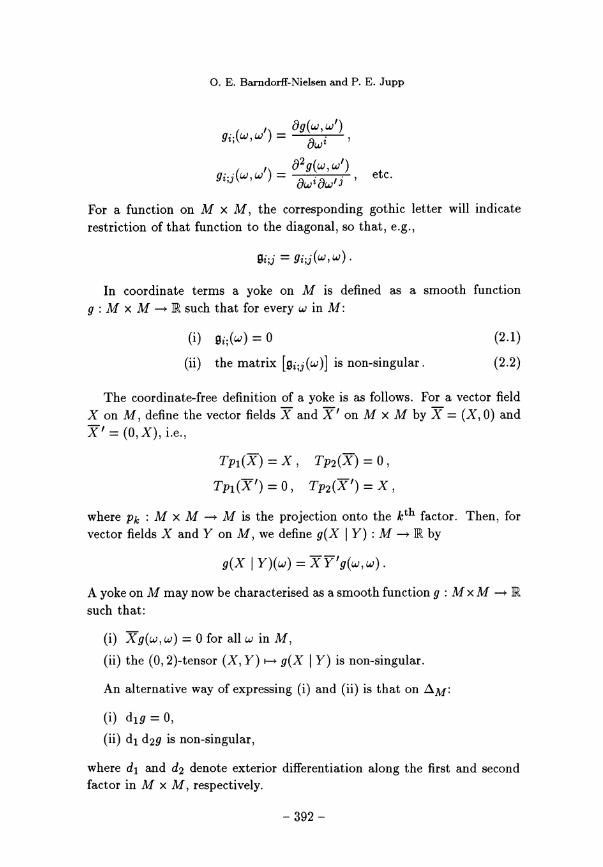
For a function on M x M, the corresponding gothic letter will indicaterestriction of that function to the diagonal, so that, e.g.,

In coordinate terms a yoke on M is defined as a smooth function

g : M x M -~ M such that for every w in M:

The coordinate-free definition of a yoke is as follows. For a vector fieldX on M, define the vector fields X and X ’ on M x M by X = (X, 0) andX ~ _ (o, X), i.e., >

where pk : M x M - M is the projection onto the kth factor. Then, forvector fields X and Y on M, we define ~ Y) M --~ R by

A yoke on M may now be characterised as a smooth function g : M x lV~ -~ Rsuch that:

(i) Xg(v, c~) = 0 for all w in M,

(ii) the (0, 2)-tensor (X, Y) ~ is non-singular.

An alternative way of expressing (i) and (ii) is that on a~:

(i) (ii) d1 d2g is non-singular,

where d1 and d2 denote exterior differentiation along the first and secondfactor in M x M, respectively.

Example The simplest example of a yoke is the function g defined

by

For all 03C9’, the function 03C9 ~ g(03C9,03C9’) has a (unique) maximum = 03C9’,so that (2.1) holds. Since ~gi~~ (w)~ is the identity matrix, (2.2) holds. Somegeneralisations of this example are given in Examples 5.1-5.3.Two of the most important geometric objects given by a yoke are a

(possibly indefinite) Riemannian metric and a one-parameter family oftorsion-zero affine connections. The metric is the (0,2)-tensor (X, Y) ~

( ~’), given in coordinate form by the matrix (gi~~~. For a in ?, thea

a-connection ~ is defined by

0where V is the Levi-Civita connection of the metric and T is given by

g(TxY ( Z)(W ) = X Y’ Z’g(c~, c~) - Y Z X ’g(cv, w) .a

Note that T is a ( 1, 2)-tensor. The lowered Christoffel symbols of V at ware given by

and the (0,3)-tensor corresponding to T is the "skewness" tensor withelements

For applications to statistics of the metric and the a-connections of expectedand observed likelihood yokes, see Amari [2], Barndorff-Nielsen ([6], [8]) andMurray and Rice ([21]).A normalised yoke is a yoke satisfying the additional condition

Except where explicitly stated otherwise, we shall consider only normalisedyokes. For any yoke g, the corresponding normalised yoke is the yoke 9defined by

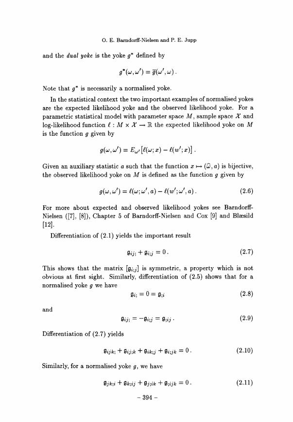
and the dual yoke is the yoke g* defined by

Note that g* is necessarily a normalised yoke.In the statistical context the two important examples of normalised yokes

are the expected likelihood yoke and the observed likelihood yoke. For a

parametric statistical model with parameter space M, sample space X and

log-likelihood function £ : M x X -~ M the expected likelihood yoke on Mis the function g given by

Given an auxiliary statistic a such that the function .c ~ a) is bijective,the observed likelihood yoke on M is defined as the function g given by

For more about expected and observed likelihood yokes see Barndorff-

Nielsen ([7], [8]), Chapter 5 of Barndorff-Nielsen and Cox [9] and Blaesild[12].

Differentiation of (2.1) yields the important result

This shows that the matrix is symmetric, a property which is not

obvious at first sight. Similarly, differentiation of (2.5) shows that for anormalised yoke g we have

Differentiation of (2.7) yields

Similarly, for a normalised yoke g, we have

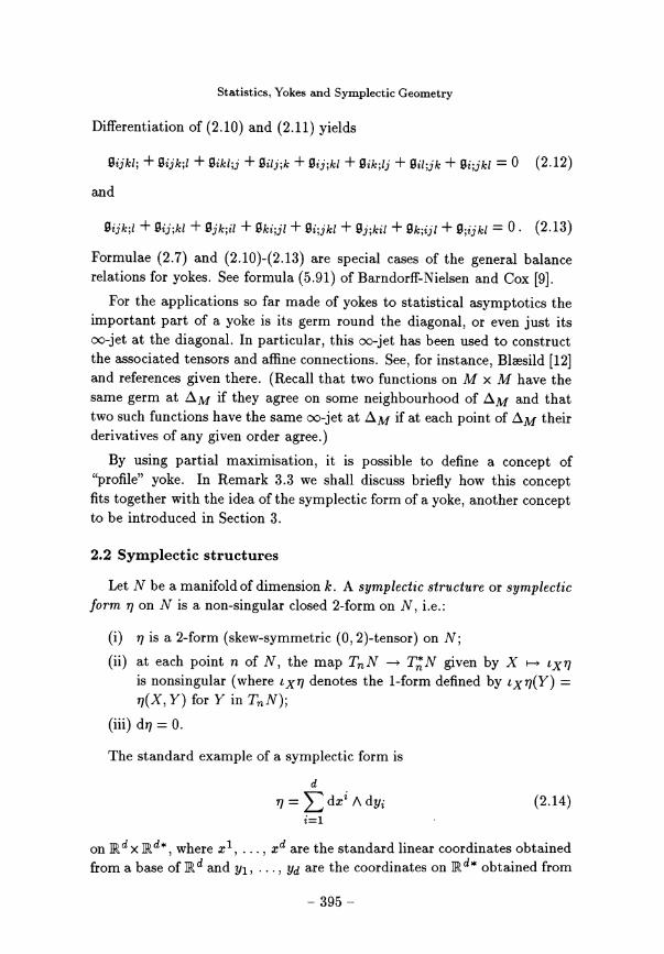
Differentiation of (2.10) and (2.11) yields

Formulae (2.7) and (2.10)-(2.13) are special cases of the general balancerelations for yokes. See formula (5.91) of Barndorff-Nielsen and Cox [9].

For the applications so far made of yokes to statistical asymptotics theimportant part of a yoke is its germ round the diagonal, or even just itsoo-jet at the diagonal. In particular, this oo jet has been used to constructthe associated tensors and affine connections. See, for instance, Blaesild [12]and references given there. (Recall that two functions on M x M have thesame germ at A~- if they agree on some neighbourhood of A~- and thattwo such functions have the same oo jet at A~- if at each point of 0~ theirderivatives of any given order agree.)

By using partial maximisation, it is possible to define a concept of

"profile" yoke. In Remark 3.3 we shall discuss briefly how this conceptfits together with the idea of the symplectic form of a yoke, another conceptto be introduced in Section 3.

2.2 Symplectic structures

Let N be a manifold of dimension k. A symplectic structure or symplecticform ?y on N is a non-singular closed 2-form on N, i.e.:

(i) ?y is a 2-form (skew-symmetric (0, 2)-tensor) on N;(ii) at each point n of N, the map TnN ~ Tn N given by X ~ X~

is nonsingular (where X~ denotes the 1-form defined by =

Y) for Y in TnN);(iii) d?? = 0.

The standard example of a symplectic form is

on where ... , xd are the standard linear coordinates obtainedfrom a base of and y1, ... yd are the coordinates on obtained from

the dual base. Locally, this is the only example of a symplectic form, becauseDarboux’s Theorem (e.g. Abraham and Marsden [1, p. 175]) states that a2-form ~ on N is a symplectic form if and only if round each point of Nthere is some coordinate system ..., xd, ..., yd) in which (2.14)holds. Note that this implies that k is necessarily even, k = 2d, and thatthe d-fold exterior product

is nowhere zero and so is a volume on N.

Formula (2.14) can be used on manifolds more general than Rd. If

x1, ..., xd are coordinates on a manifold M and y1, ..., yd are correspond-ing dual coordinates on the fibres of T*M then (2.14) defines a canonicalsymplectic form r~ on the total space T*M of the cotangent bundle of M.The symplectic form q can also be derived from the canonical 1-form 00 onT*M given by

for every v in TT*M. Here TT* M : TT*M -~ T*M denotes the projectionmap of the tangent bundle of T*M and : TT*M - T M denotesthe tangent map of TM : T * M ~ M. . In terms of the coordinates

..., xd, y1, ..., yd) on T*M, the canonical 1-form is

Remark 2.1.2014 Aspects of symplectic structures such as:

(i) existence, i.e., determining when a given closed 2-form can bedeformed into a symplectic structure,

(ii) classification, i.e., determining when two symplectic forms are equiv-alent,

(iii) the study of Lagrangian manifolds (submanifolds of maximal dimen-sion on which the restriction of ~ is zero),

appear to be mainly of mathematical/mechanical interest and not of anydirect statistical relevance (in this connection, see e.g. McDuff [20] andWeinstein [25]-[26]).

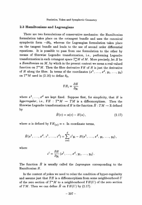
2.3 Hamiltonians and Lagrangians

There are two formulations of conservative mechanics: the Hamiltonianformulation takes place on the cotangent bundle and uses the canonicalsymplectic form whereas the Lagrangian formulation takes placeon the tangent bundle and leads to the use of second order differentialequations. It is possible to pass from one formulation to the other bymeans of fibrewise Legendre transformation, i.e., performing Legendretransformation in each cotangent space ofM. More precisely, let H bea Hamiltonian on M, by which in the present context we mean a real-valuedfunction on T*M. . Then the fibre derivative FH of H is just the derivativeof H along the fibre. In terms of the coordinates (~ 1, ..., xd, , ... Yd)on T* M used in (2.16) to define ?o,

where ... , xd are kept fixed. Suppose first, for simplicity, that H ishyperregular, i.e., FH : T*M - TM is a diffeomorphism. Then thefibrewise Legendre transformation of H is the function ~ : TM 2014~ M definedby

where a is defined by = v. In coordinate terms,

where

The function if is usually called the Lagrangian corresponding to theHamiltonian H.

In the context of yokes we need to relax the condition of hyper-regularityand assume just that FH is a diffeomorphism from some neighbourhood Uof the zero section of T*M to a neighbourhood FH(U) of the zero sectionof T M . Then we can define H on F H ( U ) by (2 .17) .

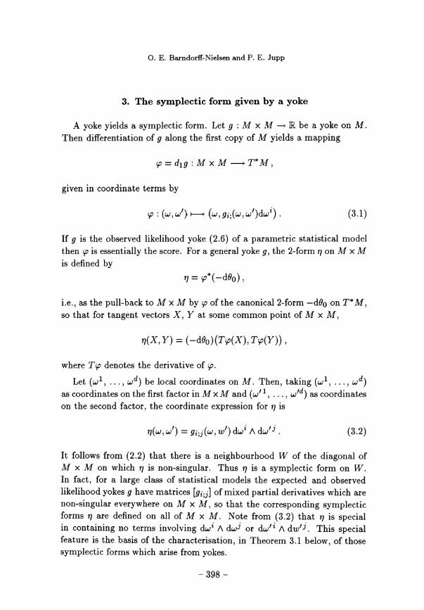
3. The symplectic form given by a yoke

A yoke yields a symplectic form. Let yoke on M.Then differentiation of g along the first copy of M yields a mapping

given in coordinate terms by

If g is the observed likelihood yoke (2.6) of a parametric statistical modelthen 03C6 is essentially the score. For a general yoke g, the 2-form ~ on M x Mis defined by

i.e.) as the pull-back to M x M by p of the canonical 2-form on T*M, ,so that for tangent vectors X, Y at some common point of M x M,

where Tp denotes the derivative of p.

Let (c,~ 1, ... , w d ) be local coordinates on M. . Then, taking (c,v 1, ... , c~ d )as coordinates on the first factor in M x M and (c~‘ 1, ... , w‘d) as coordinateson the second factor, the coordinate expression for q is

It follows from (2.2) that there is a neighbourhood W of the diagonal ofM x M on which ~ is non-singular. Thus ~ is a symplectic form on W. .In fact, for a large class of statistical models the expected and observedlikelihood yokes g have matrices [9i;j] of mixed partial derivatives which arenon-singular everywhere on M x M, so that the corresponding symplecticforms ~ are defined on all of M x M. Note from (3.2) that ~ is specialin containing no terms involving dW2 A or dw~ A . This specialfeature is the basis of the characterisation, in Theorem 3.1 below, of thosesymplectic forms which arise from yokes.

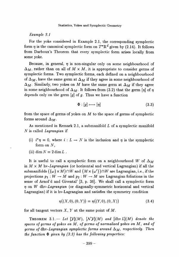
Example 3.1

For the yoke considered in Example 2.1, the corresponding symplecticform r~ is the canonical symplectic form on given by (2.14). It followsfrom Darboux’s Theorem that every symplectic form arises locally fromsome yoke.

Because, in general, r~ is non-singular only on some neighbourhood ofrather than on all of M x M, it is appropriate to consider germs of

symplectic forms. Two symplectic forms, each defined on a neighbourhoodhave the same germ at 0394M if they agree in some neighbourhood of

Similarly, two yokes on M have the same germ at 0~ if they agreein some neighbourhood of It follows from (3.2) that the germ ~r~~ of r~depends only on the germ [g] of g. Thus we have a function

from the space of germs of yokes on M to the space of germs of symplecticforms around

As mentioned in Remark 2.1, a submanifold L of a symplectic manifoldN is called Lagrangian if

(i) = 0, where z : : L ~ N is the inclusion and ~ is the symplecticform on N,

(ii) dim N = 2 dim L .

It is useful to call a symplectic form on a neighbourhood W of AMin M x M hv-Lagrangian (or horizontal and vertical Lagrangian) if all thesubmanifolds ~~w~ x M) n Wand (M x ~w~~) n Ware Lagrangian, i.e., if theprojections pi : : W -~ M and p2 : W - M are Lagrangian foliations in thesense of Arnol’d and Givental’ [3, p. 36]. We shall call a symplectic formr~ on W dhv-Lagrangian (or diagonally-symmetric horizontal and verticalLagrangian) if it is hv-Lagrangian and satisfies the symmetry condition

for all tangent vectors X, Y at the same point of M.

THEOREM 3.1.- Let [Y](M), and [dhv L](M) denote the

spaces of germs of yokes on M, of germs of normalised yokes on M, and ofgerms of dhv-Lagrangian symplectic forms around respectively. Thenthe function given by (3.3) has the following properties:

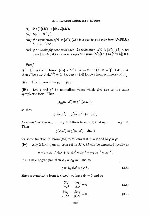
(i) ~ : [yJ (M) --~ [dhv L](M);~ [9] _ ~ ~

(iii ) the restriction to [Ny]{M) is a one-to-one map from [NyJ{M)to [dhv L](M);

(iv ) if M is simply-connected then the restriction of ~ to maps

onto [dhv L](M) and so is a bijection from to [dhv L](M).

Proof

(i) If c is the inclusion (~w~ x M) n W -~ W or (M x ~c~~~) n W -~ Wthen dcv2 A = 0. Property (3.4) follows from symmetry of gi;j.

(ii) This follows from gi; j = g2; j .

(iii) Let g and g ~ be normalised yokes which give rise to the same

symplectic form. Then

so that

for some functions ..., ad. It follows from (2.1) that a1 = ... = ad = 0.Then

for some function Q. From (2.5) it follows that /3 = 0 and so g = g’.

(iv) Any 2-form ~ on an open set in M x M can be expressed locally as

If ~ is dhv-Lagrangian then aij = Cij = 0 and so

Since a symplectic form is closed, we have d1J = 0 and so

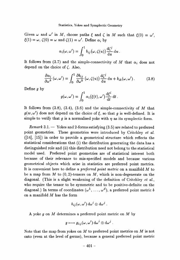
Given 03C9 and w’ in M, choose paths 03BE and ( in M such that 03BE(0) = 03C9’,~(1) = w, ~(o) = W and ~(1) = c,~’. Define ai by

It follows from (3.7) and the simple-connectivity of M that ai does notdepend on the choice of (. Also,

Define g by

It follows from (3.8), (3.4), (3.6) and the simple-connectivity of M thatg(w, c,~’) does not depend on the choice of ~, so that g is well-defined. It is

simple to verify that g is a normalised yoke with r~ as its symplectic form.

Remark 3.1. - Yokes and 2-forms satisfying (3.5) are related to preferredpoint geometries. These geometries were introduced by Critchley et al.

([14], [15]) in order to provide a geometrical structure which reflects thestatistical considerations that (i) the distribution generating the data has adistinguished role and (ii) this distribution need not belong to the statisticalmodel used. Preferred point geometries are of statistical interest bothbecause of their relevance to mis-specified models and because variousgeometrical objects which arise in statistics are preferred point metrics.It is convenient here to define a preferred point metric on a manifold M tobe a map from M to (0,2)-tensors on M, which is non-degenerate on thediagonal. (This is a slight weakening of the definition of Critchley et al.,who require the tensor to be symmetric and to be positive-definite on thediagonal.) In terms of coordinates (c,~ 1, ... , w d ), a preferred point metric bon a manifold M has the form

A yoke g on M determines a preferred point metric on M by

Note that the map from yokes on M to preferred point metrics on M is notonto (even at the level of germs), because a general preferred point metric

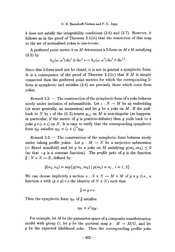
b does not satisfy the integrability conditions (3.6) and (3.7). However, itfollows as in the proof of Theorem 3.1(iii) that the restriction of this mapto the set of normalised yokes is one-to-one.

A preferred point metric b on M determines a 2-form on M x M satisfying(3.5) by ....

Since this 2-form need not be closed, it is not in general a symplectic form.It is a consequence of the proof of Theorem 3.1(iv) that if M is simplyconnected then the preferred point metrics for which the corresponding 2-form is symplectic and satisfies (3.4) are precisely those which come fromyokes.

Remark 3.2. . - The construction of the symplectic form of a yoke behavesnicely under inclusion of submanifolds. Let : N ~ M be an embedding(or more generally, an immersion) and let g be a yoke on M. If the pull-back to N by t of the (0,2)-tensor 9i;j on M is non-singular (as happens,in particular, if the metric of g is positive-definite) then g pulls back to ayoke g o (t x t) on N. It is easy to verify that the corresponding symplecticform r~~ satisfies r~~ = (t x c~ .

Remark 3.3. - The construction of the symplectic form behaves nicelyunder taking profile yokes. Let p : : M - N be a surjective submersion

(= fibred manifold) and let g be a yoke on M satisfying 0

(so that -g is a contrast function). The profile yoke of g is the function9 N x defined by

We can choose implicitly a section s : N x N ~ M x M of p x p (i.e., afunction s with (p x p) o s the identity of N x N) such that

Then the symplectic form r~~ of 9 satisfies

For example, let M be the parameter space of a composite transformationmodel with group G, let p be the quotient map p : : M - M/G, and letg be the expected likelihood yoke. Then the corresponding profile yoke

g is -7, , where I is the Kullback-Leibler profile discrimination consideredby Barndorff-Nielsen and Jupp [10]. The tensors and on M/Gobtained by applying Blaesild’s [12] general construction to the yoke g arethe transferred Fisher information p!i and the transferred skewness tensorpiD of Barndorff-Nielsen and Jupp ~10~.

Remark 3.4.- A rather different connection between statistics and

symplectic structures is given by Friedrich [17]. His construction requiresa manifold M, a vector field X on M and an X-invariant volume form Aon M. These give rise to a 2-form r~ on P(M, A), the space of probabilitymeasures on M which are absolutely continuous with respect to A. If X hasa dense orbit then ~ is a symplectic form on P(M, a). .

4. Some uses of the symplectic form of a yoke

In symplectic geometry important ways in which a symplectic structurer~ is used are:

(i) to raise and lower tensors;

(ii) to transform (the derivatives of) real-valued functions into vectorfields;

(iii) to provide a volume H, thus enabling integration over the manifold(in mechanics, over the phase space, i.e., the cotangent space).

We now apply these to the symplectic form r~ of a yoke g on M. Recallthat ~ is defined on some neighbourhood W of 0394M in M x M.

4.1 Raising and lowering tensors

A symplectic form q enables raising and lowering of tensors in thesame way that a Riemannian metric does. In particular, the "musical

isomorphism" {(, which raises 1-forms to vector fields, and its inverse D (whichlowers vector fields to 1-forms) are defined by

for 1-forms a and vector fields X and Y. For the symplectic form (3.2) ofa yoke, the coordinate expressions of # and Dare

where is the (2.0)-tensor inverse to The construction in Section 5

of the Lagrangian of a yoke can be expressed in terms of }t; see (5.2).

4.2 The vector field of a yoke

A yoke g on M gives rise as follows to a vector field Xg on W. . The

derivative dg of g is a 1-form. Raising this using )} yields the vector field= Xg . In coordinate terms, Xg (v, w~) is given by

By Liouville’s Theorem on locally Hamiltonian flows (see, e.g., Abraham

and Marsden [1, pp. 188-189]), the flow of Xg preserves the volume Q on Wdefined by (2.15). If g is an observed likelihood yoke, then the vector field

Xg describes a joint evolution of the parameter and the observation.

The vector field Xg can be used to differentiate functions. Let h be

a real-valued function on M x M. Then the derivative of h along Xg is

dh(Xg ). An alternative expression for dh(Xg ) is

where ~h, g~ is the Poisson bracket (with respect to the symplectic form r~of g ) defined by

(See, e.g., Abraham and Marsden [1, p. 192].) It is clear from (4.3) that{g, g~ = 0. This suggests that one way of comparing two normalised yokesh and g is by their Poisson bracket. In coordinate terms we have

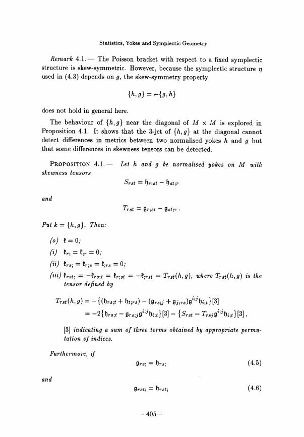
Remark 4.1.2014 The Poisson bracket with respect to a fixed symplecticstructure is skew-symmetric. However, because the symplectic structure qused in (4.3) depends on g, the skew-symmetry property

does not hold in general here.

The behaviour of ~h, g~ near the diagonal of M x M is explored inProposition 4.1. It shows that the 3-jet of ~1~, g~ at the diagonal cannotdetect differences in metrics between two normalised yokes hand g butthat some differences in skewness tensors can be detected.

PROPOSITION 4.1.- Let h and g be normalised yokes on M withskewness tensors

Then:

~ t=0;

~ ~r; _ ~;r = ~ i_ = = ~i= Wrs;t = = = g), where g) is the

tensor defined by

[3] indicating a sum of three terms obtained by appropriate permu-tation of indices.

Furthermore, if

then

Proof. - Part (o) is immediate from (4.4) and (2.8). Differentiating(4.4) with respect to 03C9 and applying (2.8) yields (i). Repeated differentiationof (i) then shows that k satisfies (2.9)-(2.11). Differentiating (4.4) twiceand three times with respect to c~, using Leibniz’ rule for differentiation of

products. and applying (2.8), (2.9) and (2.10), we obtain (ii) and

Differentiation of (ii) now yields (iii).Differentiation of (4.5) together with (4.6) and (2.9)-(2.11) yields

from which (4.7) follows.

Differentiating (4.4) four times with respect to w, using Leibniz’ rule fordifferentiation of products, and applying (4.10), we obtain

Differentiation of (4.7) now yields (4.8). D

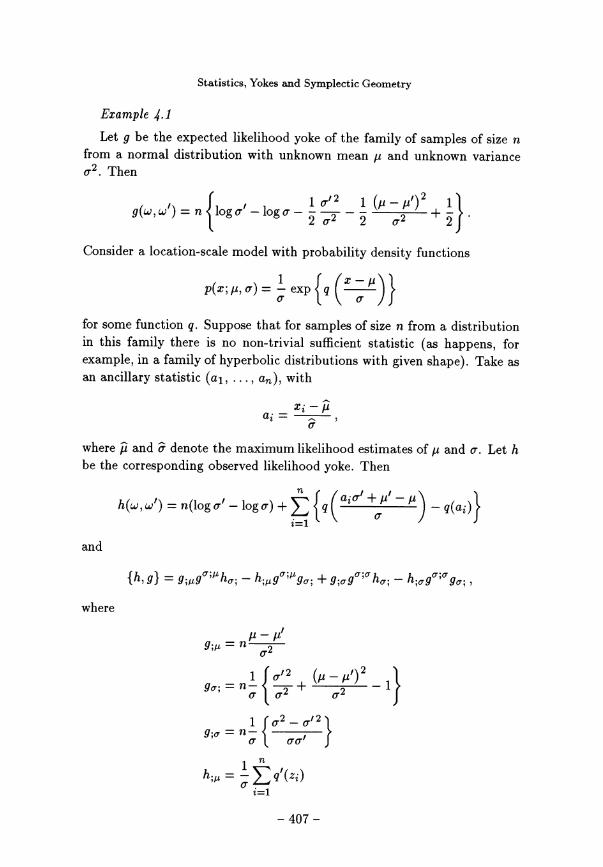
Example 4.1

Let g be the expected likelihood yoke of the family of samples of size nfrom a normal distribution with unknown mean p and unknown variance0"2. Then

Consider a location-scale model with probability density functions

for some function q. Suppose that for samples of size n from a distributionin this family there is no non-trivial sufficient statistic (as happens, for

example, in a family of hyperbolic distributions with given shape). Take asan ancillary statistic ... , an ) , with

where and ? denote the maximum likelihood estimates of p and c-. Let hbe the corresponding observed likelihood yoke. Then

where

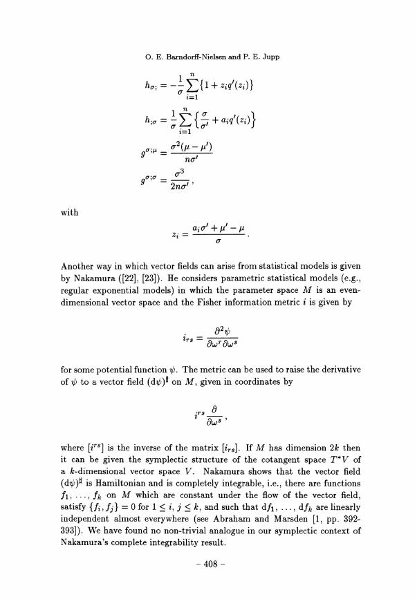
with

Another way in which vector fields can arise from statistical models is givenby Nakamura ([22], [23]). He considers parametric statistical models (e.g.,regular exponential models) in which the parameter space M is an even-dimensional vector space and the Fisher information metric i is given by

for some potential function ~. The metric can be used to raise the derivativeof 03C8 to a vector field (d’lj;)ij on M, given in coordinates by

where is the inverse of the matrix . If M has dimension 2k then

it can be given the symplectic structure of the cotangent space T*V ofa k-dimensional vector space V. Nakamura shows that the vector field

(d~)~ is Hamiltonian and is completely integrable, i.e., there are functionsf1, ... , fk on M which are constant under the flow of the vector field,satisfy = 0 for 1 i, j k, and such that df1, ..., d fk are linearlyindependent almost everywhere (see Abraham and Marsden [1, pp. 392-393]). We have found no non-trivial analogue in our symplectic context ofNakamura’s complete integrability result.

4.3 The volume of a yoke

Recall from (2.15) that a yoke g on M gives rise to a volume Q on someneighbourhood W of the diagonal in M x M. For many yokes of statisticalinterest W can be taken to be all of M x M. However, for a general yoke,W will be a proper subset of M x M. The main way in which volumes areused is as objects to be integrated over the manifolds on which they live,so in such cases there is no obvious choice of manifold over which Q shouldbe integrated. (One possibility is to integrate S2 over the maximal such Wbut the interpretation of the value of this integral is not clear.)An alternative way of using the volume Q is to compare it with other

volumes on W, , in particular with the restriction to W of the geometricmeasure obtained from the metric of g. More precisely, the yoke g gives a(possibly indefinite) Riemannian metric on M and so a volume on M givenin coordinate terms as

where [ . denotes the absolute value of the determinant. The correspondingproduct measure on M x M is the volume with coordinate form

It follows from (2.9) that (4.11) can also be written as

Since Q is given in coordinate form as d! w~ ) I volume (4.11 ) can bewritten as d! M, where the function h : W ~ R is given in coordinate formby

Note that, in general, h is not a yoke. However, h can be used to obtainfurther yokes from g. . For any real A define M x M - R by

Since h = 1 on the diagonal, the following proposition shows that is a

normalised yoke with the same metric as g. Note that the germs at 0~ ofhand depend only on the germ of g.

PROPOSITION 4.2. - Let g be a normalised yoke on M and h : M x M --~

II8 be any function such that h = 1 on the diagonal 0~. Then

(i) the product hg is a normalised yoke on M having the same metricas g;

(ii) the function

satisfies

Proof. - These are simple calculations. D

Remark 4.2. - Note that if k in Proposition 4.2 satisfies also

the matrix + is non-singular {4.14)

then k is rather like a yoke but need not satisfy (2.1). Note also that

conditions (4.13) and (4.14) provide a generalisation of the concept of anormalised yoke. Also, in contrast to the definition of a yoke, (4.13) and(4.14) involve the two arguments in a symmetrical way.

Remark 4.3. - Let k be a function on M x M satisfying (4.14). Definegk : M x M -~ 1I8 by

Then gk is a normalised yoke on M. .

Remark 4.4. - One context in which the "adjustment factor" h of (4.12)occurs in statistics is in a variant of the p*-formula for the distribution ofthe score

, _ ~ _ ~ ,

A suitable starting point for this is the p*-formula

for the distribution of the maximum likelihood estimator. Here [ )[ is the

determinant of the observed information matrix j = ili, a) evaluated

at ili. For an extensive discussion of this formula and its applicationssee Barndorff-Nielsen and Cox [9]. The expression v | a) d1 ... represents a volume on M. Changing the variable in (4.15) from ~ to thescore s* gives the p*-formula

for the distribution of s*. The expression p* (s*; w a) dsl ~ ~ ~ dsd representsa volume on the cotangent space to M at w . Now j defined by

= is an inner-product on TWM, so that j-1 is an inner-producton The geometric measure of j -1 is a measure on represented

Then _u..

is a ratio of measures on TWM. Let j-1~2 be any square root of j-1 anddefine the standardised score s* by

Barndorff-Nielsen [8, sect. 7.3] derived

as an approximation to the density ofs*. . Note that p* (s*; W a) is (4.16).Define h M x l~l -~ R by

Since the observed likelihood yoke (2.6) is g, given by

we have, neglecting an additive constant,

where h is the "adjustment factor" defined in (4.12). From Proposition 4.2,k satisfies (4.13). By differentiating (4.12) twice, we obtain

where

is one of the tensors introduced by Blaesild [12].

5. The Lagrangian of a yoke

Let g be a yoke on M. As discussed after equation (3.2), we can choosea neighbourhood W of 0~ in M x M such that the restriction to W of p,where p is defined by (3.1), is a diffeomorphism onto . We define the

Hamiltonian of g as the function H : y~(W ) ~ Il8 given by

In coordinate terms, H is given by

where w’ is determined by

It follows from (2.2) that we can choose W such that the restriction top(W) of the fibre derivative FH of H is a diffeomorphism onto its image.By the definition in subsection 2.3, the Lagrangian corresponding to H isfI R, the fibrewise Legendre transform of H. However, itis convenient to refer to

as the Lagrangian of g. An alternative expression for g is

In coordinate terms, 9 is given by

Because the restriction to W of FH is a diffeomorphism, it follows from(5.1) that 9 is equivalent to H. Since 9 is similar to g in being a functiondefined on a neighbourhood of A~f in M x M, it is often convenient to

consider 9 rather than fl.

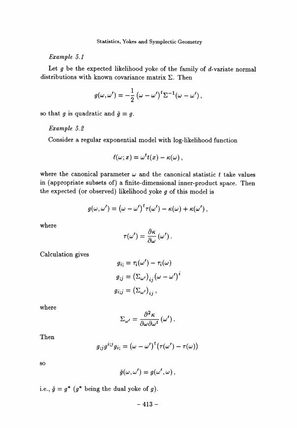
Example 5.1

Let g be the expected likelihood yoke of the family of d-variate normaldistributions with known covariance matrix £. Then

so that g is quadratic and g = g .

Example Consider a regular exponential model with log-likelihood function

where the canonical parameter (w) and the canonical statistic t take valuesin (appropriate subsets of) a finite-dimensional inner-product space. Thenthe expected (or observed) likelihood yoke g of this model is

where

Calculation gives

where

Then

so

i.e., 9 = g* (g* being the dual yoke of g).

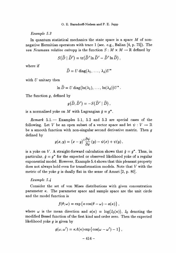
Example 5. 3

In quantum statistical mechanics the state space is a space M of non-

negative Hermitian operators with trace 1 (see. e.g., Balian [4, p. 75]). Thevon Neumann relative entropy is the function S M x M ~ R defined by

where if

with U unitary then

The function g, defined by

is a normalised yoke on M with Lagrangian 9 = g* .

Remark 5.1. Examples 5.1, 5.2 and 5.3 are special cases of the

following. Let V be an open subset of a vector space and let 03C8 : be a smooth function with non-singular second derivative matrix. Then gdefined by

is a yoke on V. A straight-forward calculation shows that 9 = g*. Thus, inparticular, 9 = g* for the expected or observed likelihood yoke of a regularexponential model. However, Example 5.4 shows that this pleasant propertydoes not always hold even for transformation models. Note that V with themetric of the yoke g is dually flat in the sense of Amari [2, p. 80].

Example 5..~Consider the set of von Mises distributions with given concentration

parameter K. The parameter space and sample space are the unit circleand the model function is

where w is the mean direction and a(/;) = Io denoting themodified Bessel function of the first kind and order zero. Then the expectedlikelihood yoke g is given by

where A(K) = with I1 denoting the modified Bessel function ofthe first kind and order 1. Putting

and using straight-forward calculations, we obtain

so

Since g(w, w’) = g(w’, w), we have g = g* and so g ~ g* . Also,

so

and ~ g.

Remark 5.2.2014 The first term on the right hand side of (5.3) is reminis-cent of

which is the (quadratic) score statistic in the case where g is an observedor expected likelihood yoke. Thus

can be regarded as a "mixed score statistic" and

can be regarded as a "dual score statistic" .

Now we consider how close 9 is to g and show that 9 is closer to g* thanto g.

THEOREM 5.1. Let g be a normalised yoke and denote by g* the dual

yoke of g. Define the "skewness tensor" Trst of the yoke g by

as in ~~.,~~ and denote by ~{‘~}, ~* ~a~ and the a-connections of g, g*and g, respectively. Following Blaesild define the tensor r s;tu by

as in (/.1 7). Then:

(I) § is a normalised yoke;

(it) § has ihe same metric as g and g*;

(iii) r st; " glst; " gr st; - TTSt

r s;t * gls;t " gTsjt + Tr st

#r;st = gl;st = gr;st - Tr st

;r st " g*;r st " g;r st + Tr st i

(iv) #r;st - st;r = -Tr st;

(y ) Q(") = v* (") = v(~");(Vi) r stu; - g*r stu; " -%rs;tu [6]

r st;u - " %rs;tu [6]

r s;tu - g2s;tu " -%rs;tu [6]r ;stu - * %rs;tu [6]

;r stu - g*;r stu * -%rs;tu [6] .

Proof. - Differentiation of (5.3) with respect to wr yields

and so

by (2.8). Differentiation of (5.4) with respect to ws and evaluation at 03C9 = w’gives

Similarly,

Since g is a normalised yoke, we see from (2.9) that

and so (i) and (ii) follow. Evaluating the second derivative of (5.4) = c,~~,we obtain

From (2.10), (2.11) and (2.4), we have

Combining (5.8) with (5.9) and (5.10) gives

Differentiation of (5.5), (5.6) and (5.7) gives

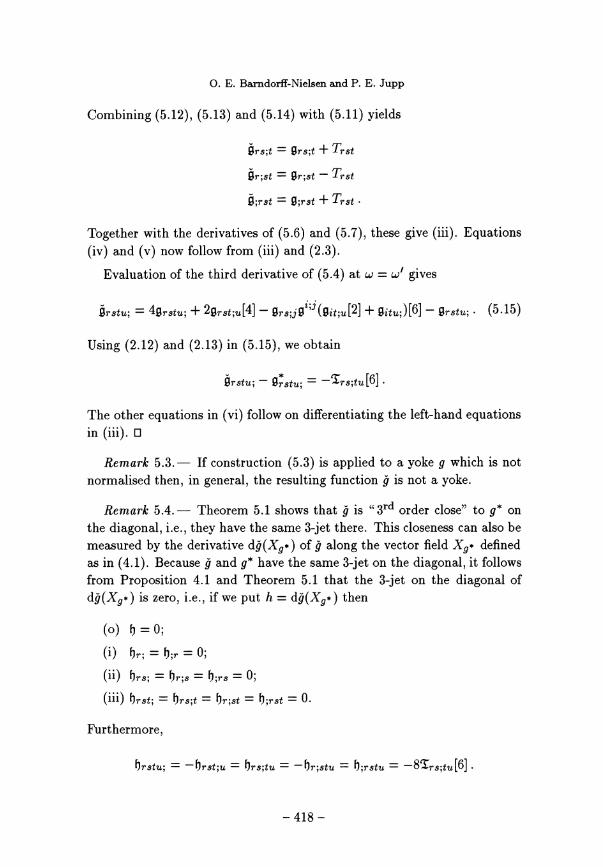
Combining (5.12), (5.13) and (5.14) with (5.11) yields

Together with the derivatives of (5.6) and (5.7), these give (iii). Equations(iv) and (v) now follow from (iii) and (2.3).

Evaluation of the third derivative of (5.4) at w = f.J)’ gives

Using (2.12) and (2.13) in (5.15), we obtain

The other equations in (vi) follow on differentiating the left-hand equationsin (iii). 0

Remark 5.3. - If construction (5.3) is applied to a yoke g which is notnormalised then, in general, the resulting function g is not a yoke.

Remark 5.4. - Theorem 5.1 shows that g is " 3rd order close" to g* onthe diagonal, i.e., they have the same 3-jet there. This closeness can also bemeasured by the derivative dg(lYg* ) of g along the vector field Xg* definedas in (4.1). Because g and g* have the same 3-jet on the diagonal, it followsfrom Proposition 4.1 and Theorem 5.1 that the 3-jet on the diagonal of

dg(Xg* ) is zero, i.e., if we put h = dg{Xg* ) then

Furthermore,

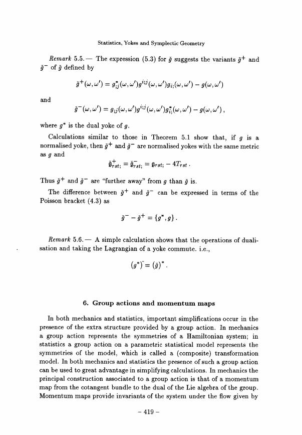
Remark 5.5. - The expression (5.3) for 9 suggests the variants g+ andg - of g defined by

where g* is the dual yoke of g.Calculations similar to those in Theorem 5.1 show that, if g is a

normalised yoke, then g+ and g- are normalised yokes with the same metricas g and

Thus g+ and g- are "further away" from g than 9 is.The difference between g+ and g- can be expressed in terms of the

Poisson bracket (4.3) as

Remark 5.6. - A simple calculation shows that the operations of duali-sation and taking the Lagrangian of a yoke commute. i.e.,

6. Group actions and momentum maps

In both mechanics and statistics, important simplifications occur in thepresence of the extra structure provided by a group action. In mechanicsa group action represents the symmetries of a Hamiltonian system; instatistics a group action on a parametric statistical model represents thesymmetries of the model, which is called a (composite) transformationmodel. In both mechanics and statistics the presence of such a group actioncan be used to great advantage in simplifying calculations. In mechanics theprincipal construction associated to a group action is that of a momentummap from the cotangent bundle to the dual of the Lie algebra of the group.Momentum maps provide invariants of the system under the flow given by

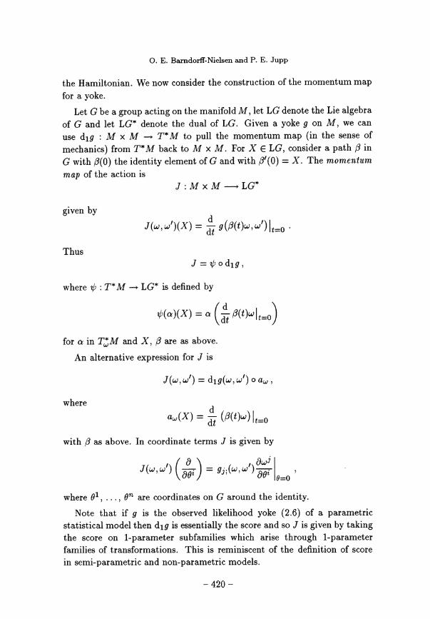
the Hamiltonian. We now consider the construction of the momentum map

for a yoke.Let G be a group acting on the manifold M, let LG denote the Lie algebra

of G and let LG* denote the dual of LG. Given a yoke g on M, we canuse dig : M x M - T*M to pull the momentum map (in the sense of

mechanics) from T*M back to M x M. For X E LG, consider a path Q inG with /3(0) the identity element of G and with /?~(0) = X. The momentummap of the action is

given by

Thus

where 9 : T* M ~ LG* is defined by

for a in T~M and X, /3 are as above.

An alternative expression for J is

where

with {3 as above. In coordinate terms J is given by

where 81, ..., en are coordinates on G around the identity.Note that if g is the observed likelihood yoke (2.6) of a parametric

statistical model then d1g is essentially the score and so J is given by takingthe score on 1-parameter subfamilies which arise through 1-parameterfamilies of transformations. This is reminiscent of the definition of score

in semi-parametric and non-parametric models.

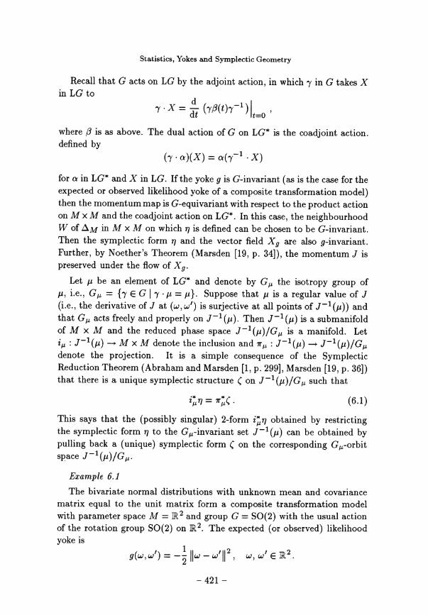
Recall that G acts on LG by the adjoint action, in which y in G takes XinLGto

where Q is as above. The dual action of G on LG* is the coadjoint action.defined by

for a in LG* and X in LG. If the yoke g is G-invariant (as is the case for theexpected or observed likelihood yoke of a composite transformation model)then the momentum map is G-equivariant with respect to the product actionon M x M and the coadjoint action on LG*. In this case, the neighbourhoodW of OM in M x M on which ~ is defined can be chosen to be G-invariant.Then the symplectic form q and the vector field Xg are also g-invariant.Further, by Noether’s Theorem (Marsden [19, p. 34]), the momentum J ispreserved under the flow of Xg.

Let p be an element of LG* and denote by G~ the isotropy group ofp, i.e., G~ - ~-y E G ~ y ~ ~c = ~~. Suppose that p is a regular value of J(i.e., the derivative of J at (w,w’) is surjective at all points of J-1 (~c)) andthat G~ acts freely and properly on J-1 (~). Then J-1 (~c) is a submanifoldof M x M and the reduced phase space is a manifold. Let

: J-1 (~c) --~ ~l x M denote the inclusion and J-1 (~c) -~ denote the projection. It is a simple consequence of the SymplecticReduction Theorem (Abraham and Marsden [1, p. 299], Marsden [19, p. 36])that there is a unique symplectic structure ( on J-1 (~C)/G~ such that

This says that the (possibly singular) 2-form obtained by restrictingthe symplectic form r~ to the G~-invariant set ~7-1 (~c) can be obtained bypulling back a (unique) symplectic form ( on the corresponding Gu-orbitspace

Example 6.1

The bivariate normal distributions with unknown mean and covariancematrix equal to the unit matrix form a composite transformation modelwith parameter space M = JR 2 and group G = SO(2) with the usual actionof the rotation group SO(2) on The expected (or observed) likelihoodyoke is

..

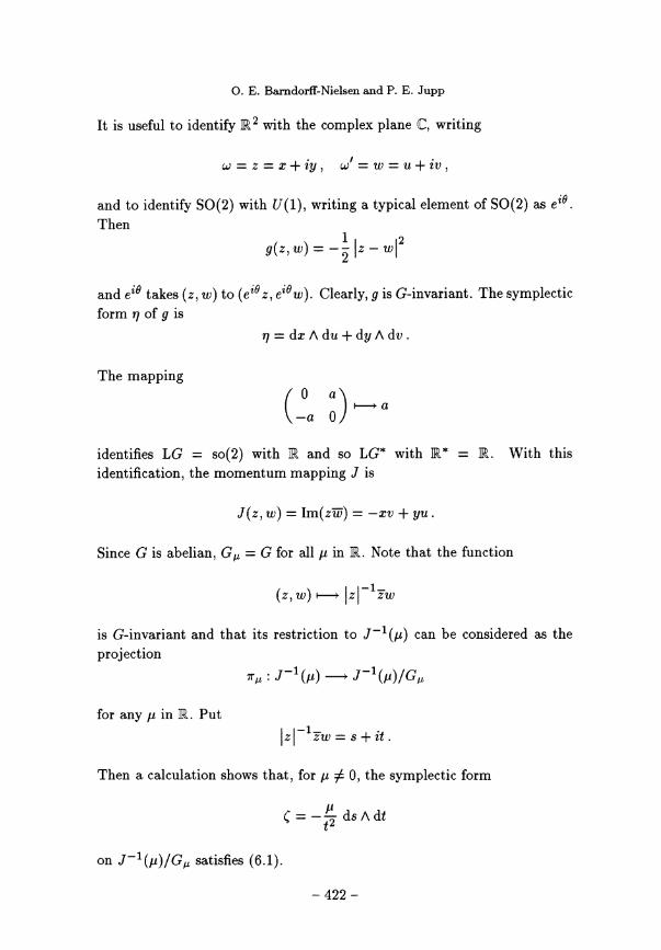
It is useful to identify R2 with the complex plane C, writing

and to identify SO(2) with !7(1), writing a typical element of SO(2) as eZe.Then

and eZe takes (z, w) to e28w~. Clearly, g is G-invariant. The symplecticform x~ of g is

The mapping

identifies LG = so(2) with R and so LG* with R* = R. With this

identification, the momentum mapping J is

Since G is abelian, G~ = G for all J.t in M. Note that the function

is G-invariant and that its restriction to J-1 (~) can be considered as theprojection

for any in M. Put

Then a calculation shows that, for J.l ~ 0, the symplectic form

on satisfies (6.1).

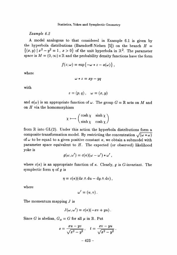
Example 6. 2

A model analogous to that considered in Example 6.1 is given bythe hyperbola distributions (Barndorff-Nielsen [5]) on the branch H ={ (x, y) I x2 - y2 = 1, x > 0~ of the unit hyperbola in R~. The parameterspace is M = (0, oo) x R and the probability density functions have the form

where

with

and is an appropriate function of cv . The group G = R acts on M andon H via the homomorphism

from M into GL(2). Under this action the hyperbola distributions form acomposite transformation model. By restricting the concentration (w * w)of 03C9 to be equal to a given positive constant 03BA, we obtain a submodel with

parameter space equivalent to H. The expected (or observed) likelihoodyoke is

where C(K) is an appropriate function of K. Clearly, g is G-invariant. Thesymplectic form 1J of g is

where

The momentum mapping J is

Since G is abelian, G,~ = G for all Jl in M. Put

Then the function

is G-invariant and its restriction to J-1 (~c) can be considered as the

projection

for any in R. A calculation shows that, 0, the symplectic form

on satisfies (6.1).

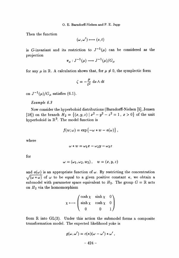
Example 6.3

Now consider the hyperboloid distributions (Barndorff-Nielsen [5], Jensen[18]) on the branch H2 = ~ (x, y, z) ~ x2 _ y2 _ z2 = 1, x ~ 0} of the unithyperboloid in The model function is

where

for

and a( w) is an appropriate function of w. By restricting the concentrationof w to be equal to a given positive constant K, we obtain a

submodel with parameter space equivalent to H2. The group G = R actson H2 via the homomorphism

from R into GL(3). Under this action the submodel forms a compositetransformation model. The expected likelihood yoke is

where C(K) is an appropriate function of K. Because the product * and thefunction c are G-invariant, so is the yoke g. The symplectic form r~ of g is

where

The momentum mapping J is

Since G is abelian, G = G for all in M. The function

is G-invariant and its restriction to J-1 (~c) can be considered as the

projection

for any p in ?. A calculation shows that the symplectic form

on J ~(~)/(9~ satisfies (6.1).

AcknowledgementThis research was supported in part by a twinning grant in the European

Community Science programme and by a network contract in the EuropeanUnion HCM programme.

References

[1] ABRAHAM (R.) and MARSDEN (J. E.) .2014 Foundations of Mechanics, 2nd ed.,Addison-Wesley, Redwood City (1978).

[2] AMARI (S.-I.) .2014 Differential-Geometrical Methods in Statistics, Lecture Notesin Statistics, Springer-Verlag, Heidelberg, 28 (1985).

[3] ARNOL’D (V. I.) and GIVENTAL’ (A. B.) .2014 Symplectic Geometry, In "Dynam-ical Systems IV: Symplectic Geometry and its Applications", Encyclopaedia ofMathematical Sciences (V. I. Arnol’d and S. P. Novikov, eds), Springer-Verlag,Berlin, 4 (1990), pp. 1-136.

[4] BALIAN (R.) .2014 From Microphysics, to Macrophysics, Springer-Verlag, Berlin, 1(1991).

[5] BARNDORFF-NIELSEN (O. E.) .2014 Hyperbolic distributions and distributions on

hyperbolae, Scand. J. Statist. 5 (1978), pp. 151-157.

[6] BARNDORFF-NIELSEN (O. E.) .2014 Likelihood and observed geometries, Ann.Statist. 14 (1986), pp. 856-873.

[7] BARNDORFF-NIELSEN (O. E.) .2014 Differential geometry and statistics: some

mathematical aspects, Indian J. Math. 29 (1987), pp. 335-350.

[8] BARNDORFF-NIELSEN (O. E.) .2014 Parametric Statistical Models and Likelihood,Lecture Notes in Statistics, Springer-Verlag, Heidelberg, 50 (1988).

[9] BARNDORFF-NIELSEN (O. E.) and Cox (D. R.) .2014 Inference and Asymptotics,Chapman &#x26; Hall, London (1994).

[10] BARNDORFF-NIELSEN (O. E.) and JUPP (P. E.) .- Differential geometry, profilelikelihood, L-sufficiency and composite transformation models, Ann. Statist. 16

(1988), pp. 1009-1043.

[11] BARNDORFF-NIELSEN (O. E.) and JUPP (P. E.) .2014 Yokes and symplectic struc-tures, J. Statist. Planning and Infce. 63 (1997), pp. 133-146.

[12] BLÆSILD (P.) . 2014 Yokes and tensors derived from yokes, Ann. Inst. Statist. Math.43 (1991), pp. 95-113.

[13] COMBET (E.) .2014 Intégrales Exponentielles, Lecture Notes in Mathematics,Springer-Verlag, Berlin, 937 (1982).

[14] CRITCHLEY (F.), MARRIOTT (P. K.) and SALMON (M.) .2014 Preferred pointgeometry and statistical manifolds, Ann. Statist. 21 (1993), 1197-1224.

[15] CRITCHLEY (F.), MARRIOTT (P. K.) and SALMON (M.) .2014 Preferred pointgeometry and the local differential geometry of the Kullback-Leibler divergence,Ann. Statist. 22 (1994), pp. 1587-1602.

[16] EGUCHI (S.) .2014 Second order efficiency of minimum contrast estimation in acurved exponential family, Ann. Statist. 11 (1983), pp. 793-803.

[17] FRIEDRICH (T.) . 2014 Die Fisher-Information und symplectische Strukturen, Math.Nachr. 153 (1991), pp. 273-296.

[18] JENSEN (J. L.) .2014 On the hyperboloid distribution, Scand. J. Statist. 8 (1981),pp. 193-206.

[19] MARSDEN (J. E.) .2014 Lectures on Mechanics, London Mathematical SocietyLecture Note Series, Cambridge University Press, Cambridge, 174 (1992).

[20] MCDUFF (D.) .2014 Examples of symplectic structures, Invent. Math. 89 (1987),pp. 13-36.

[21] MURRAY (M. K) and RICE (J. W.) .2014 Differential Geometry and Statistics,Chapman &#x26; Hall, London (1993).

[22] NAKAMURA (Y.) . 2014 Completely integrable gradient systems on the manifolds ofGaussian and multinomial distributions, Japan J. Industr. Appl. Math. 10

(1993), pp. 179-189.

- 427 -

Statistics, Yokes and Symplectic Geometry

[23] NAKAMURA (Y.) .2014 Gradient systems associated with probability distributions,Japan J. Industr. Appl. Math. 11 (1994), pp. 21-30.

[24] SKOVGAARD (I. M.) .2014 On the density of minimum contrast estimators, Ann.Statist. 18 (1990), pp. 779-789.

[25] WEINSTEIN (A.) .2014 Symplectic manifolds and their Lagrangian submanifolds,Adv. Math. 6 (1971), pp. 329-346.

[26] WEINSTEIN (A.) . 2014 Lectures on Symplectic Manifolds, AMS Regional ConferenceSeries in Mathematics, American Mathematical Society, Providence, RhodeIsland, 29 (1977).