hepth@xxx/9704037CERN-TH/97-63Miami TH/1/97

ANL-HEP-PR-97-10

Integrable Symplectic Trilinear Interaction Terms for Matrix Membranes

Thomas Curtright§, David Fairlie\1, and Cosmas Zachos¶

§ Department of Physics, University of Miami, Box 248046, Coral Gables, Florida 33124, USAcurtright@phyvax.ir.Miami.edu

\ Theory Division, CERN, CH-1211 Geneva 23, SWITZERLANDDavid.Fairlie@cern.ch

¶ High Energy Physics Division, Argonne National Laboratory, Argonne, IL 60439-4815, USAzachos@hep.anl.gov

Abstract

Cubic interactions are considered in 3 and 7 space dimensions, respectively, for bosonic membranesin Poisson Bracket form. Their symmetries and vacuum configurations are discussed. Their associatedfirst order equations are transformed to Nahm’s equations, and are hence seen to be integrable, for the3-dimensional case, by virtue of the explicit Lax pair provided. The constructions introduced also applyto commutator or Moyal Bracket analogues.

Introduction

A proposal for non-perturbative formulation of M-theory [1] has led to a revival of matrix membranetheory [2, 3]. Symmetry features of membranes and their connection to matrix models [3, 4, 5, 6, 7] havebeen established for quite some time. Effectively, infinite-N quantum mechanics matrix models presented asa restriction out of SU(∞) Yang-Mills theories amount to membranes, by virtue of the connection betweenSU(N) and area-preserving diffeomorphisms (Sdiff) generated by Poisson Brackets, in which “colour”algebra indices Fourier-transform to “membrane” sheet coordinates. The two are underlain and linked byMoyal Brackets.

Below, we consider novel Poisson Bracket interactions for a bosonic membrane embedded in 3-space

LIPB =1

3εµνκXµ{Xν , Xκ}, (1)

which are restrictions of the Moyal Bracket generalization

LIMB =1

3εµνκXµ{{Xν , Xκ}}, (2)

which, in turn, also encompasses the plain matrix commutator term

LIC =1

3εµνκXµ[Xν , Xκ] . (3)

The structure of (1) may be recognized as that of the interaction term εijlφiεµν∂µφ

j∂νφj of the 2-

dimensional SO(3) pseudodual chiral σ-model of Zakharov and Mikhailov [8]—this is a limit [9] of the

1On research leave from the University of Durham, U.K.

WZWN interaction term, where the integer WZWN coefficient goes to infinity while the coupling goes tozero, such that the product of the integer with the cube of the coupling is kept constant. The structure of(3) is also linked to what remains of the gauge theory instanton density,

K0 = εµνκTrAµ

(∂νAκ −

1

4[Aν , Aκ]

), (4)

in the standard space-invariant limit (where the first term vanishes). (N.B. This interaction may becontrasted to the one which appears in a different model [10].) There is some formal resemblance tomembrane interaction terms introduced in [11], in that case a quartic in the Xµ’s, which, in turn, reflectthe symplectic twist of topological terms [12] for self-dual membranes. Unlike those interactions, the cubicterms considered here do not posit full Lorentz invariance beyond 3-rotational invariance: they are merelybeing considered as quantum mechanical systems with internal symmetry. One may expect this fact tocomplicate supersymmetrization.

We then also introduce analogous trilinear interactions for membranes embedded in 7-space, which alsoevince similarly interesting properties.

In what follows, after a brief review of some matrix membrane technology, we discuss the symmetryfeatures of the new terms, the symmetry of the corresponding vacuum configurations, and describe classicalconfigurations of the Nahm type, which we find to be integrable, as in the conventional membrane models.Our discussion will concentrate on Poisson Brackets, but the majority of our results carry over to theMoyal Bracket and commutator cases, by dint of the underlying formal analogy. Subtler considerations ofspecial features for various membrane topologies are not discussed here, and may be addressed as in [13].Nontrivial boundary terms, e.g. of the type linked to D-branes, are not yet addressed.

Review and Notation

Poisson Brackets, Moyal Brackets, and commutators are inter-related derivative operators, sharingsimilar properties such as Leibniz chain rules, integration by parts, associativity (so they obey the Jacobiidentity), etc. Much of their technology is reviewed in [14, 5, 7, 15].

Poisson Brackets act on the “classical phase-space” of Fourier-transformed colour variables, with mem-brane coordinates ξ = α, β,

{Xµ, Xν} =∂Xµ

∂α

∂Xν

∂β−∂Xµ

∂β

∂Xν

∂α. (5)

This might be effectively regarded as the infinitesimal canonical transformation on the coordinates ξ ofXν , generated by ∇Xµ × ∇, s.t. (α, β) 7→ (α − ∂Xµ/∂β , β + ∂Xµ/∂α), which preserves the membranearea element dαdβ. This element is referred to as a symplectic form and the class of transformations thatleaves it invariant specifies a symplectic geometry; the area preserving diffeomorphisms are dubbed Sdiff .

PBs correspond to N →∞ matrix commutators. But there is a generalization which covers both finiteand infinite N . The essentially unique associative generalization of PBs is the Moyal Bracket [14],

{{Xµ, Xν}} =1

λsin

(λ∂

∂α

∂

∂β′− λ

∂

∂β

∂

∂α′

)Xµ(ξ)Xν(ξ′)

∣∣∣∣∣ξ′=ξ

. (6)

For λ = 2π/N , ref [5] demonstrates that the Moyal bracket is essentially equivalent to the commutatorof SU(N) matrices (or subalgebras of SU(N), depending on the topology of the corresponding membranesurface involved in the Fourier-transform of the colour indices [7, 13]). In the limit λ→ 0, the Moyal bracketgoes to the PB (i.e. λ may be thought of as h). Thus, PBs are seen to represent the infinite N limit. Thistype of identification was first noted by Hoppe on a spherical membrane surface [3]; the foregoing Moyallimit argument was first formulated on the torus [5], but extends naturally to other topologies [5, 7, 13].

Refs [4] utilize the abovementioned identification of SU(∞) with Sdiff on a 2-sphere, to take the large Nlimit of SU(N) gauge theory and produce membranes. This procedure was found to be more transparent

on the torus [7]: the Lie algebra indices Fourier-conjugate to surface coordinates, and the fields are rescaledFourier transforms of the original SU(N) fields. The group composition rule for them is given by the PBsand the group trace by surface integration,

[Aµ, Aν ] 7→ {aµ, aν} ; (7)

Fµν = ∂µAν − ∂νAµ + [Aµ, Aν ] 7→ fµν(α, β) = ∂µaν − ∂νaµ + {aµ, aν} ; (8)

TrFµνFµν 7→ −N3

64π4

∫dαdβ fµν(α, β) fµν(α, β). (9)

But the large N limit need not be taken to produce sheet actions. The Lagrangian with the MoyalBracket supplanting the Poisson Bracket is itself a gauge-invariant theory, provided that the gauge trans-formation also involves the Moyal instead of the Poisson bracket:

δaµ = ∂µΛ− {{Λ, aµ}} , (10)

and hence, by virtue of the Jacobi identity,

δfµν = −{{Λ, fµν}} . (11)

colour invariance then follows,

δ

∫dαdβ fµνfµν = −2

∫dαdβ fµν{{Λ, fµν}} = 0 . (12)

The relevant manipulations are specified in [7], and the last equality is evident by integrations by parts,where the surface term is discarded, or nonexistent if the colour membrane surface is closed. (But note thistopological term may be nontrivial for D-membranes.) For λ = 2π/N , this is equivalent to the conventionalSU(N) commutator gauge theory.

Consider the SU(∞) Yang Mills Lagrangian and dimensionally reduce all space dependence [3], leavingonly time dependence, while preserving all the colour-Fourier-space (membrane coordinates ξ = α, β)dependence of the gauge fields, which are now denoted Xµ(t, α, β). Fix the gauge to X0 = 0. TheYang-Mills lagrangian density reduces to the bosonic membrane lagrangian density

LPB =1

2(∂tX

µ)2 −1

4{Xµ, Xν}2. (13)

The PB is also the determinant of the tangents to the membrane, so the conventional “potential term” wasidentified in [7] as the Schild-Eguchi string lagrangian density [16] (sheet area squared instead of area),{Xµ,Xν}{Xµ,Xν}. (It can be seen that the equations of motion of such a string action contain those ofNambu’s action.)

Note that, fixing the gauge X0 = 0 preserves the global colour invariance, i.e. with a time-independentparameter Λ(α, β). The action is then invariant under

δXµ = {Λ, Xµ}. (14)

By Noether’s theorem, this implies the time invariance of the colour charge,

QΛ =

∫dαdβ Λ(α, β) {∂tX

µ, Xµ}. (15)

The same also works for the Moyal case [7]. The corresponding Moyal Schild-Eguchi term was utilizedto yield a “star-product-membrane” [15],

LMB =1

2(∂tX

µ)2 −1

4{{Xµ, Xν}}2, (16)

invariant underδXµ = {{Λ, Xµ}}. (17)

As outlined, this includes the commutator case,

LC =1

2(∂tX

µ)2 −1

4[Xµ, Xν ]2, (18)

invariant underδXµ = [Λ, Xµ]. (19)

Discussion of the Cubic Terms for 3 Dimensions

By suitable integrations by parts, it is straightforward to check that the cubic terms (1,2,3) in the re-spective actions,

∫dtdαdβ L, are 3-rotational invariant, as well as time-translation invariant and translation

symmetric. They are also global colour invariant, as specified above.

Let us also consider a plain mass term in the action, (of the type that may arise as a remnant of spacegradients in compactified dimensions),

L3dPB =1

2(∂tX

µ)2 −1

4{Xµ, Xν}2 −

m

2εµνκXµ{Xν , Xκ} −

m2

2(Xµ)2. (20)

The second order equation of motion,

∂2tX

µ = −m2Xµ −3m

2εµνκ{Xν , Xκ} − {Xν , {Xµ, Xν}}, (21)

follows not only from extremizing the action, but also results from a first-order equation of the Nahm(self-dual) type [17], albeit complex,

∂tXµ = imXµ +

i

2εµνκ{Xν , Xκ}. (22)

These equations hold for PBs, MBs, and commutators.

For solutions of this first-order equation, the conserved energy vanishes. In general, however, suchsolutions are not real, and do not provide absolute minima for the action. Nonetheless, the lagrangiandensity can be expressed as a sum of evocative squares, since the potential in (20) is such a sum,

L3dPB =1

2(∂tX

µ)2 −1

2

(mXµ +

1

2εµνκ{Xν , Xκ}

)2

. (23)

By integration by parts in the action∫dtdαdβ L3dPB, the lagrangian density itself can then be altered to

L3dPB∼= −

1

2

(i∂tX

µ +mXµ +1

2εµνκ{Xν , Xκ}

)2

, (24)

just like the conventional bosonic membrane lagrangian density (the congruence symbol, ∼=, indicates equiv-alence up to surface terms, which, e.g., vanish for a closed surface; again, consideration of D-membraneswould proceed separately). The complex-conjugate versions of the above are equally valid.

Vacuum Configurations

The minimum of the conventional matrix membrane trough potential favors alignment of the Xµs. Themass parameter introduced above parameterizes a partial trough symmetry breaking [18], but does not lift“dilation” invariance, seen as follows.

The static (t-independence) minima for the action (vacuum configurations) are solutions of

mXµ +1

2εµνκ{Xν , Xκ} = 0 . (25)

The previously considered case, m = 0, is easily solved by “colour-parallel” configurations. But for m 6= 0,the static solutions must lie on a 2-sphere, since from the previous equation

Xµ∂Xµ

∂α= 0 = Xµ∂X

µ

∂β, (26)

soXµXµ = R2 , (27)

an unspecified constant. (Hence εµνκXµ{Xν , Xκ} = −2mR2.) However, from (25), note that both m andalso R, the scale of the Xµs, can be absorbed in the membrane coordinates ξ and will not be specified bythe solution of (25).

Indeed, solving for one coordinate component on this sphere, say

X(Y,Z) = ±√R2 − Y 2 − Z2 , (28)

reduces the three equations (25) to one. Namely,

{Z, Y } = m√R2 − Y 2 − Z2 , (29)

on the positive X branch (m 7→ −m on the negative X branch). This last equation is solved by

Z = α, Y =√R2 − α2 sin(mβ) . (30)

One can then interpret mβ as the usual azimuthal angle around the Z-axis. Hence, −π/2 ≤ mβ ≤ π/2and −R ≤ α ≤ R covers the X ≥ 0 hemisphere completely. The other hemisphere is covered completely bythe negative X branch. Since R is not fixed, it amounts to an unlifted residual trough dilation degeneracy.

All static solutions are connected to this explicit one by rescaling R and exploiting the equation’sarea-preserving diffeomorphism invariance for ξ = (α, β).

Nahm’s Equation and Lax Pairs

The first order equation, (22), simplifies upon changing variables to τ = eimt/m and Xµ = eimtYµ, andreduces to the conventional PB version [19] of Nahm’s equation [17],

∂τYµ =

1

2εµνκ{Y ν , Y κ}. (31)

This has real solutions, and can be linearized by Ward’s transformation [19]. However, the action (23) doesnot reduce to the conventional one upon these transformations. (Likewise, the second order equations ofmotion only reduce to ∂2

τYµ = {Y ν , {Y µ, Y ν}}+ 3

τ (∂τYµ − εµνκ

2 {Yν , Y κ}).)

Moreover, note

∂τYµ∂τY

µ =∂(Y 1, Y 2, Y 3)

∂(τ, α, β), (32)

∂τYµ∂ξY

µ = 0. (33)

One may further utilize the cube root of unity, ω = exp(2πi/3), (note ω(ω − 1) is pure imaginary) torecast (31),

L ≡ ωY 1 + ω2Y 2 + Y 3 , L = ω2Y 1 + ωY 2 + Y 3 , M ≡ Y 1 + Y 2 + Y 3 , (34)

ω(ω − 1) ∂τL = {M , L} , ω(ω − 1) ∂τL = −{M , L} , ω(ω − 1) ∂τM = {L ,L} , (35)

which thus yields an infinite number of complex time-invariants,

Qn =

∫dαdβ Ln , (36)

for arbitrary integer power n, as the time derivative of the integrand is a surface term. (This is in completeanalogy with the standard case of commutators.) This is linked to classical integrability, as discussed next.

Eqs (35) amount to one complex and one real equation, but these can further be compacted into justone by virtue of an arbitrary real spectral parameter ζ, introduced in [20]:

H ≡i

√2ω(ω − 1)

(ζL−

L

ζ

), K ≡ i

√2M + ζL+

L

ζ, (37)

∂τK = {H,K} . (38)

(Note the wave solution H = α, L = f(β + τ).) This Lax pair, analogous to [20], likewise leads to aone-parameter family of time-invariants,

Qn(ζ) =

∫dαdβ Kn , (39)

and a Lax isospectral flow,

K ≡ ∇K ×∇, H ≡ ∇H ×∇, ∇ ≡(∂

∂α,∂

∂β

), (40)

such that:∂τK = HK−KH . (41)

As a consequence, the spectrum of K is preserved upon time evolution by the (pure imaginary) H:

∂τψ = Hψ, (42)

since time-differentiatingKψ = λψ (43)

and applying the above yields

(∂τλ) ψ = (∂τK)ψ +K∂τψ − λ ∂τψ = 0 . (44)

This isospectral flow then provides integrability [8] for (22), as in the case of the conventional Nahmequation.

This discussion also carries over to plain commutators or Moyal Brackets as well, with suitable adap-tations [5].

Duality and Implicit Solution of the (PB) Nahm Equation

Ward [19] has solved eq (31) implicitly through twistor linearization.

Another solution procedure for the construction of a wide class of solutions to (31) may be found byinterchanging the roles of dependent and independent variables; the equations then take the form

∂τ

∂Y 1=

∂α

∂Y 2

∂β

∂Y 3−

∂α

∂Y 3

∂β

∂Y 2, (45)

together with cyclic permutations, i.e.∂µτ = εµνρ∂να ∂ρβ . (46)

Cross-differentiation produces integrability conditions

∂µ(∂κα ∂µβ − ∂µα ∂κβ) = 0. (47)

Another evident consistency condition is∂2τ = 0 , (48)

but this will be guaranteed by the integrability of those equations. Having found α, β in terms ofY 1, Y 2, Y 3, the solution for τ follows by quadratures.

Evidently, solutions of these dual equations

∂µf = εµνρ∂νg ∂ρh , (49)

for f(Y 1, Y 2, Y 3) produce constants of the motion∫d2ξ f , beyond those already found by the Lax proce-

dure, for the original equation (31), in illustration of a phenomenon noted in [21], as it is straightforwardto verify that df/dτ = {g, h}. Actually, f need only solve Laplace’s equation (48): any harmonic functionf(Y 1, Y 2, Y 3) yields a conserved density for (31), by also satisfying (49). By virtue of Helmholtz’s theorem,a divergenceless 3-vector ∇f is representable as a curl of another vector A. On the other hand, an arbitrary3-vector can also be represented in terms of three scalars by means of the Clebsch decomposition of thatvector as A = g∇h+∇u. In fact, the problem of solving the inverse Nahm equation (45) is equivalent todetermining the Clebsch decomposition of an arbitrary vector.

A class of solutions can be found by postulating a simple dependence on Y 3; with the Ansatz

τ = f(Y 1, Y 2), α = e−mY3g(Y1,Y2), β = emY3

h(Y1,Y2), (50)

it is seen that the equations are satisfied, provided g is an arbitrary function of h,

g = φ(h), (51)

as well asτ = <F (Y 1 + iY 2), mgh = =F (Y 1 + iY 2) , (52)

for an arbitrary analytic function F , since these combinations must satisfy the Cauchy-Riemann conditions.

Membrane Embedding in 7 Dimensions

Remarkably, the same type of term may also be introduced for a membrane embedded in 7 space di-mensions. A self-dual (antisymmetric) 4-tensor in 8 dimensions, fµνρσ was invoked [22] as an 8-dimensionalanalogue of the 4-dimensional fully antisymmetric tensor εµνρσ. Some useful technology for the manipula-tion of this tensor (which has 35 nonzero components and is invariant under a particular SO(7) subgroupof SO(8)) can also be found in [23]; in particular, the identity

f0µνκf0µλρ = fνκλρ + δνλδκρ − δκλδνρ . (53)

By analogy with (31), one can postulate a first order equation

∂τYµ −

f0µνκ

2{Y ν , Y κ} = 0 . (54)

The indices run from µ = 1 to µ = 7, since we are working in a gauge where Y 0 = 0. The second orderequation arising from iteration of (54), by virtue of the above identity as well as the Jacobi identity is

∂ττYµ = −{{Y µ, Y ν}, Y ν} . (55)

This arises from the lagrangian density

L7dPB =1

2(∂τY

µ)2 +1

4{Y µ, Y ν}2 . (56)

As in the 3-dimensional case, this action is a sum of squares up to a mere surface term,

1

2

(∂τY

µ −f0µνκ

2{Y ν , Y κ}

)2

= L7dPB − f0µνκ∂τY

µ∂αYν∂βY

κ ∼= L7dPB. (57)

Apparent extra quartic terms in this lagrangian density have, in fact, vanished by virtue of the identity,

{f, g}{h, k}+ {f, h}{k, g}+ {f, k}{g, h} ≡ 0, (58)

which holds for Poisson Brackets on a 2-dimensional phase-space—but not for commutators nor MoyalBrackets2. This cancellation works at the level of the lagrangian density for the PB case. However, notethat even for ordinary matrices the corresponding term would vanish in the traced action, by the cyclicityof the trace pitted against full antisymmetry,

fµνκρTrXµXνXκXρ = 0 . (59)

Likewise, the corresponding interaction for Moyal Brackets,

fµνκρ∫d2ξ {{Xµ,Xν}}{{Xκ,Xρ}}, (60)

is forced by associativity to reduce to a surface term, vanishing unless there are contributions from sur-face boundaries or D-membrane topological numbers involved. (Shortcuts for the manipulation of suchexpressions underlain by ?-products can be found in, e.g. [15].) The cross terms involving time derivativesare expressible as divergences, as in the 3-dimensional case, and hence give rise to possible topologicalcontributions.

As a result, (54) is the Bogomol’nyi minimum of the action (56) with the bottomless potential.

As in the case of 3-space, the conventional membrane signs can now be considered (for energy boundedbelow), and a symmetry breaking term m introduced, to yield

L7dPB∼= −

1

2

(−i∂tX

µ +mXµ +f0µνκ

2{Xν , Xκ}

)2

. (61)

This model likewise has 7-space rotational invariance, and its vacuum configurations are, correspond-ingly, 2-surfaces lying on the spatial 6-sphere embedded in 7-space: XµXµ = R2. But, in addition, becauseof (53), these surfaces on the sphere also satisfy the trilinear constraint

fλµνκXµ{Xν , Xκ} = 0 , (62)

for λ 6= 0. (For λ = 0 this trilinear is −2mR2.)

Higher-dimensional Analogues

The system of equations (54) does not appear to readily yield integrability properties. However, itmay be extended to a 9-dimensional system—or, equivalently, a 10-dimensional one if ∂τY

µ is replaced by{Y 0, Y µ}. This different system, though it breaks the 9-dimensional rotational invariance, is integrableby virtue of the additional six constraints imposed on the system.

Writing out the system (54) explicitly and augmenting it with two more variables, Y 8, Y 9, gives riseto the equations

2D. Fairlie and A. Sudbery, 1988, unpublished. It follows from ε[jkδl]m = 0, whence ε[jkεl]m = 0 for these membranesymplectic coordinates.

∂τY1 = {Y 2, Y 3}+ {Y 6, Y 5}+ {Y 4, Y 7}+ {Y 8, Y 9}

∂τY2 = {Y 3, Y 1}+ {Y 4, Y 6}+ {Y 5, Y 7}

∂τY3 = {Y 1, Y 2}+ {Y 5, Y 4}+ {Y 6, Y 7}

∂τY4 = {Y 3, Y 5}+ {Y 6, Y 2}+ {Y 7, Y 1}

∂τY5 = {Y 4, Y 3}+ {Y 1, Y 6}+ {Y 7, Y 2}

∂τY6 = {Y 2, Y 4}+ {Y 5, Y 1}+ {Y 7, Y 3}

∂τY7 = {Y 1, Y 4}+ {Y 2, Y 5}+ {Y 3, Y 6}

∂τY8 = {Y 9, Y 1}

∂τY9 = {Y 1, Y 8}

0 = {Y 8, Y 2}+ {Y 3, Y 9}

0 = {Y 8, Y 3}+ {Y 9, Y 2}

0 = {Y 8, Y 6}+ {Y 5, Y 9}

0 = {Y 8, Y 5}+ {Y 9, Y 6}

0 = {Y 8, Y 4}+ {Y 7, Y 9}

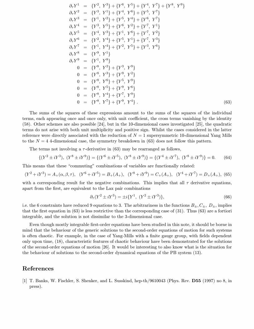
0 = {Y 8, Y 7}+ {Y 9, Y 4} . (63)

The sums of the squares of these expressions amount to the sums of the squares of the individualterms, each appearing once and once only, with unit coefficient, the cross terms vanishing by the identity(58). Other schemes are also possible [24], but in the 10-dimensional cases investigated [25], the quadraticterms do not arise with both unit multiplicity and positive sign. Whilst the cases considered in the latterreference were directly associated with the reduction of N = 1 supersymmetric 10-dimensional Yang Millsto the N = 4 4-dimensional case, the symmetry breakdown in (63) does not follow this pattern.

The terms not involving a τ -derivative in (63) may be rearranged as follows,

{(Y 2 ± iY 3), (Y 8 ± iY 9)} = {(Y 6 ± iY 5), (Y 8 ± iY 9)} = {(Y 4 ± iY 7), (Y 8 ± iY 9)} = 0. (64)

This means that these “commuting” combinations of variables are functionally related:

(Y 2 + iY 3) = A+(α, β, τ), (Y 6 + iY 5) = B+(A+), (Y 8 + iY 9) = C+(A+), (Y 4 + iY 7) = D+(A+), (65)

with a corresponding result for the negative combinations. This implies that all τ derivative equations,apart from the first, are equivalent to the Lax pair combinations

∂τ (Y 2 ± iY 3) = ±i{Y 1, (Y 2 ± iY 3)}, (66)

i.e. the 6 constraints have reduced 9 equations to 3. The arbitrariness in the functions B±, C±, D±, impliesthat the first equation in (63) is less restrictive than the corresponding case of (31). Thus (63) are a fortioriintegrable, and the solution is not dissimilar to the 3-dimensional case.

Even though mostly integrable first-order equations have been studied in this note, it should be borne inmind that the behaviour of the generic solutions to the second-order equations of motion for such systemsis often chaotic. For example, in the case of Yang-Mills with a finite gauge group, with fields dependentonly upon time, (18), characteristic features of chaotic behaviour have been demonstrated for the solutionsof the second-order equations of motion [26]. It would be interesting to also know what is the situation forthe behaviour of solutions to the second-order dynamical equations of the PB system (13).

References

[1] T. Banks, W. Fischler, S. Shenker, and L. Susskind, hep-th/9610043 (Phys. Rev. D55 (1997) no 8, inpress).

[2] P. Collins and R. Tucker, Nucl. Phys. B112 (1976) 150.

[3] J. Hoppe, M.I.T. Ph.D. Thesis (1982), in Elem. Part. Res. J. (Kyoto) 83 no.3 (1989/90).

[4] E. Floratos, J. Iliopoulos, and G. Tiktopoulos, Phys. Lett. B217 (1989) 285.B. de Wit, J. Hoppe, and H. Nicolai, Nucl. Phys. B305 [FS23] (1988) 545;J. Hoppe, Int. J. Mod. Phys. A4 (1989) 5235;E. Bergshoeff, E. Sezgin, Y. Tanii, and P. Townsend, Ann. Phys. 199 (1990) 340.

[5] D. Fairlie, P. Fletcher, and C. Zachos, Phys. Lett. B218 (1989) 203;D. Fairlie and C. Zachos, Phys. Lett. B224 (1989) 101.

[6] E. Floratos, Phys. Lett. B228 (1989) 335.

[7] D. Fairlie, P. Fletcher, and C. Zachos, J. Math. Phys. 31 (1990) 1088.

[8] V. Zakharov and A. Mikhailov, Sov. Phys. JETP 47 (1978) 1017;T. Curtright and C. Zachos, Phys. Rev. D49(1994) 5408.

[9] T. Curtright and C. Zachos, PASCOS’94, K. C. Wali (ed.), World Scientific, 1995, pp 381-390,(hep-th/9407044).

[10] J. Plebanski, M. Przanowski, and H. Garcia-Compean, Mod. Phys. Lett. A11 (1996) 663.

[11] R. Zaikov, Phys. Lett. B266 (1991) 303.

[12] B. Biran, E. Floratos, and G. Savvidi, Phys. Lett. B198 (1987) 329.

[13] N. Kim and S-J. Rey, hep-th/9701139.

[14] J. Moyal, Proc. Camb. Phil. Soc. 45 (1949) 99;D. Fairlie, Proc. Camb. Phil. Soc. 60 (1964) 581;D. Fairlie and C. Manogue, J. Phys. A24 (1991) 3807.T. Jordan and E. Sudarshan, Rev. Mod. Phys. 33 (1961) 515;J. Vey, Comment. Math. Helvetici 50 (1975) 412;P. Fletcher, Phys. Lett. B248 (1990) 323.

[15] J. Hoppe, Phys. Lett. B250 (1990) 44.

[16] A. Schild, Phys. Rev. D16 (1977) 1722 ; T. Eguchi, Phys. Rev. Lett. 44 (1980) 126.

[17] W. Nahm, Group Theoretical Methods in Physics: XIth International Colloquium, Istanbul, 1982, M.Serdaroglu and E. Inonu (eds), Springer Lecture Notes in Physics, 180, Berlin, 1983, pp 456-466.

[18] T. Curtright and T. McCarty have considered a system equivalent to the limit of X3 =constant ofthis model in an unpublished ICTP’89 talk, (http://phyvax.ir.miami.edu:8001/curtright/ictp89.html),and the latter’s unpublished University of Florida Thesis.

[19] R. Ward, Phys. Lett. B234 (1990) 81.

[20] E. Floratos and G. Leontaris, Phys. Lett. B223 (1989) 153;M. Hitchin, Comm. Math. Phys. 89 (1983) 145.

[21] D. Fairlie and I. Strachan, Physica D90 (1996) 1.

[22] E. Corrigan, C. Devchand, D. Fairlie, and J. Nuyts, Nucl. Phys. B214 (1982) 452.

[23] R. Dundarer, F. Gursey and C-H. Tze, J. Math. Phys. 25 (1984) 1496.

[24] R. Ward, Nucl. Phys. B236 (1984) 381.

[25] D. Fairlie and C. Devchand, Phys. Lett. B141 (1984) 73.

[26] S. Matinyan, G. Savvidy, and N. Ter-Arutunian Savvidy, Sov. Phys. JETP 53 (1981) 421; JETP Lett.34 (1981) 590; S. Matinyan, E. Prokhorenko, and G. Savvidy, Nucl. Phys. B298 (1988) 414.