arX

iv:0

806.

1360

v4 [

nlin

.SI]

16

Jun

2010

Integrable generalizations of Schrodinger maps and Heisenberg

spin models from Hamiltonian flows of curves and surfaces

Stephen C. Anco

Department of Mathematics, Brock University, St. Catharines, ON Canada∗

R. Myrzakulov

Department of General and Theoretical Physics,

Eurasian National University, Astana, 010008, Kazakhstan†

Abstract

A moving frame formulation of non-stretching geometric curve flows in Euclidean space is used

to derive a 1+1 dimensional hierarchy of integrable SO(3)-invariant vector models containing the

Heisenberg ferromagnetic spin model as well as a model given by a spin-vector version of the

mKdV equation. These models describe a geometric realization of the NLS hierarchy of soliton

equations whose bi-Hamiltonian structure is shown to be encoded in the Frenet equations of the

moving frame. This derivation yields an explicit bi-Hamiltonian structure, recursion operator, and

constants of motion for each model in the hierarchy. A generalization of these results to geometric

surface flows is presented, where the surfaces are non-stretching in one direction while stretching in

all transverse directions. Through the Frenet equations of a moving frame, such surface flows are

shown to encode a hierarchy of 2+1 dimensional integrable SO(3)-invariant vector models, along

with their bi-Hamiltonian structure, recursion operator, and constants of motion, describing a

geometric realization of 2+1 dimensional bi-Hamiltonian NLS and mKdV soliton equations. Based

on the well-known equivalence between the Heisenberg model and the Schrodinger map equation

in 1+1 dimensions, a geometrical formulation of these hierarchies of 1+1 and 2+1 vector models

is given in terms of dynamical maps into the 2-sphere. In particular, this formulation yields a new

integrable generalization of the Schrodinger map equation in 2+1 dimensions as well as a mKdV

analog of this map equation corresponding to the mKdV spin model in 1+1 and 2+1 dimensions.

∗Electronic address: sanco@brocku.ca†Electronic address: cnlpmyra@mail.ru

1

I. INTRODUCTION AND SUMMARY

Spin systems are an important class of dynamical vector models from both physical

and mathematical points of view. In physics such models describe nonlinear dynamics of

magnetic materials, while in mathematics they give rise to associated geometric flows of

curves where the unit tangent vector along a curve is identified with a dynamical spin

vector.

A main example [14] is the Heisenberg model for the dynamics of an isotropic ferromagnet

spin system in 1+1 dimensions. The geometric curve flow described by this SO(3)-invariant

model corresponds to the equations of motion of a non-stretching vortex filament in Eu-

clidean space. Remarkably, the vortex filament equations are an integrable Hamiltonian

system that is equivalent to the 1+1 dimensional focusing nonlinear Schrodinger equation

(NLS) through a change of dynamical variables known as a Hasimoto transformation [13].

The vortex filament equations are one example in an infinite hierarchy of non-stretching

geometric flows of space curves whose equations of motion have a well-understood integra-

bility: e.g. a Lax pair and an associated isospectral linear eigenvalue problem; an infinite

set of symmetries and constants of motion; and exact solutions with solitonic properties.

This integrability structure turns out to have a simple geometric origin. In particular, all of

these equations of motion are generated through a recursion operator that can be derived

geometrically [10, 23] from the Serret-Frenet structure equations given by a SO(3) moving

frame formulation for arbitrary non-stretching curve flows in Euclidean space, with the com-

ponents of the frame connection matrix providing the dynamical variables that appear in the

equations of motion. More recently, these SO(3) frame structure equations have been found

to geometrically encode a pair of compatible Hamiltonian operators that yield a concrete

bi-Hamiltonian structure for the equations of motion of each integrable curve flow in the

hierarchy [17].

The explicit bi-Hamiltonian form of the resulting equations of motion depends on a choice

of the SO(3) moving frame for the underlying space curve, which determines the form of the

frame connection matrix and hence yields the dynamical variables in terms of the curve. In

the case of the vortex filament equations, the dynamical variables consist of the curvature

invariant, κ, and the torsion invariant, τ , of the space curve, corresponding to the choice of

a classical Frenet frame [12] given by the unit tangent vector, unit normal and bi-normal

2

vectors, along the curve. Other geometrical choices of a moving frame can be made [2],

since there is a SO(3) gauge freedom relating any two orthonormal frames along an arbitrary

curve in Euclidean space. In particular, the Hasimoto transformation arises geometrically as

a gauge transformation from a Frenet frame to a parallel frame [7], where the frame vectors

in the normal space of the curve are chosen such that their derivative with respect to the

arclength s along the curve lies in the tangent space of the curve. This choice of frame is

unique up to rigid SO(2) rotations acting on the normal vectors by the same angle at all

points along the curve, while leaving invariant the tangent vector. The corresponding pair

of dynamical variables (defined by the connection matrix of a parallel frame) are naturally

equivalent to a single complex-valued variable u = κ exp(i∫τds) that is determined by the

curve only up to constant phase rotations u→ eiφu (where φ is independent of arclength s).

This dynamical variable u thus has the geometrical meaning [5] of a U(1) ≃ SO(2) covariant

of the space curve. Importantly, the resulting Hamiltonian structure for the equations of

motion looks simplest in terms of the covariant u, which directly incorporates the Hasimoto

transformation, rather than using the classical invariants κ and τ .

The purpose of the present paper will be to give some new applications of these ideas to

the study of integrable vector models in 1+1 and 2+1 dimensions.

Firstly, from the hierarchy of non-stretching geometric space curve flows that contains

the vortex filament equations, we derive the complete hierarchy of corresponding integrable

SO(3)-invariant vector models in 1+1 dimensions, along with their bi-Hamiltonian integra-

bility structure in explicit form. In addition to the Heisenberg model, this hierarchy will

be seen to contain a model that describes a spin-vector version of the mKdV equation.

Our results provide a new derivation of the Hamiltonian structure, recursion operator, and

constants of motion for these models.

Secondly, we extend the derivation to a geometrically analogous class of surface flows

where the surface is non-stretching in one coordinate direction while stretching in all trans-

verse directions. Such surfaces arise in a natural fashion from a spatial Hamiltonian flow

of non-stretching space curves. This generalization will be shown to give rise to a class of

2+1 dimensional NLS and mKdV soliton equations with an explicit bi-Hamiltonian struc-

ture, yielding a hierarchy of integrable SO(3)-invariant vector models in 2+1 dimensions.

In particular, this hierarchy includes 2+1 generalizations of the Heisenberg spin model and

the mKdV spin model, which were found in earlier work by one of us [15, 18–21]. Our

3

derivation here, in contrast, yields the explicit bi-Hamiltonian structure, recursion operator,

and constants of motion, which are new results for these models. We also write out the cor-

responding surface flows explicitly in terms of geometric variables given by [12] the geodesic

and normal curvatures and the relative torsion of the non-stretching coordinate lines on the

surface. The surface flow arising from the 2+1 integrable Heisenberg model will be seen to

describe a sheet of non-stretching vortex filaments in Euclidean space.

Lastly, we also derive an interesting geometric formulation of these results by viewing

the spin vector as a dynamical map into the 2-sphere in Euclidean space. This formula-

tion is based on the well-known geometrical equivalence between the Heisenberg model and

the Schrodinger map equation in 1+1 dimensions [25]. When applied to the 1+1 and 2+1

dimensional hierarchies of SO(3)-invariant vector models, our derivation yields a new inte-

grable generalization of the Schrodinger map equation in 2+1 dimensions as well as a new

mKdV analog of this map equation corresponding to the mKdV spin-vector model in 1+1

and 2+1 dimensions.

The rest of the paper is organized as follows. In section II, we review from a unified point

of view the mathematical relationships amongst 1+1 dimensional vector models, dynamical

maps into the 2-sphere, non-stretching curve flows in Euclidean space, Frenet and parallel

frames, and the Hasimoto transformation. In section III, we derive the NLS hierarchy of

soliton equations in terms of the geometrical covariant u given by the Frenet equations of

a moving parallel frame for non-stretching space curve flows. This approach directly yields

the explicit bi-Hamiltonian structure of these soliton equations, including a formula for the

Hamiltonians. As examples, the parallel-frame Frenet equations are used to show, firstly,

how the NLS equation itself corresponds geometrically to the Heisenberg spin model and

the Schrodinger map equation; and secondly, how the mKdV spin model and the mKdV

map equation arise geometrically from the next soliton equation in the NLS hierarchy.

Section IV contains several main results. We work out the equations of motion for the

space curves corresponding to the NLS hierarchy and write down the induced flows on the

curvature and torsion invariants κ, τ . Next we derive the resulting geometrical hierarchies

of vector models and dynamical map equations, along with their bi-Hamiltonian structure,

recursion operators, and constants of motion. This new derivation involves only the parallel-

frame Frenet equations plus the bi-Hamiltonian structure of the NLS hierarchy. The explicit

bi-Hamiltonian form of the Schrodinger map equation and Heisenberg model, including a

4

geometric expression for the Hamiltonians, are presented as examples.

In section V, we consider surfaces generated by a spatial Hamiltonian flow of curves with a

parallel framing in Euclidean space. The underlying Hamiltonian structure is shown to arise

naturally from the Frenet equations of the induced frame along the surface. This formulation

is then used in section VI to study surface flows expressed in terms of the covariant variable u

geometrically associated with the non-stretching space curves that foliate the surface, where

the surface is stretching in all directions transverse to these curves. We show that the bi-

Hamiltonian structure for 1+1 flows on u has a natural extension to 2+1 flows based on the

observation that the Hamiltonian operators involve only the coordinate in the non-stretching

direction on the surface. This leads to a hierarchy of 2+1 flows on u, with the starting flow

given geometrically by translations in the coordinate in the transverse direction, which yields

a 2+1 generalization of the NLS hierarchy.

The final two sections of the paper contain our main new results. In section VII, we

use the surface Frenet equations to derive the complete hierarchies of integrable 2+1 vector

models and dynamical maps arising from the 2+1 generalization of the NLS hierarchy. The

derivation yields the explicit bi-Hamiltonian structure of these two hierarchies, in addition

to their respective recursion operators and constants of motion. As examples, the integrable

generalizations of the Heisenberg model and the mKdV spin model in 2+1 dimensions are

written down in detail, as well as the corresponding new 2+1 dimensional integrable gen-

eralizations of the Schrodinger map equation and mKdV map equation. In section VIII,

we work out the equations of motion for the surface flows that correspond to the previ-

ous hierarchies. These equations are obtained by means of a different framing defined in

a purely geometrical fashion by the non-stretching coordinate direction on the surface and

the orthogonal direction of the surface normal in Euclidean space. We also discuss aspects

of both the intrinsic and extrinsic geometry of the resulting surface motions. In particular,

we obtain a recursion operator, constants of motion, and explicit evolution equations for-

mulated in terms of geometric variables given by the geodesic curvature, normal curvature,

and relative torsion of the non-stretching coordinate lines on the surface.

Some concluding remarks on future extensions of this work are given in section IX.

5

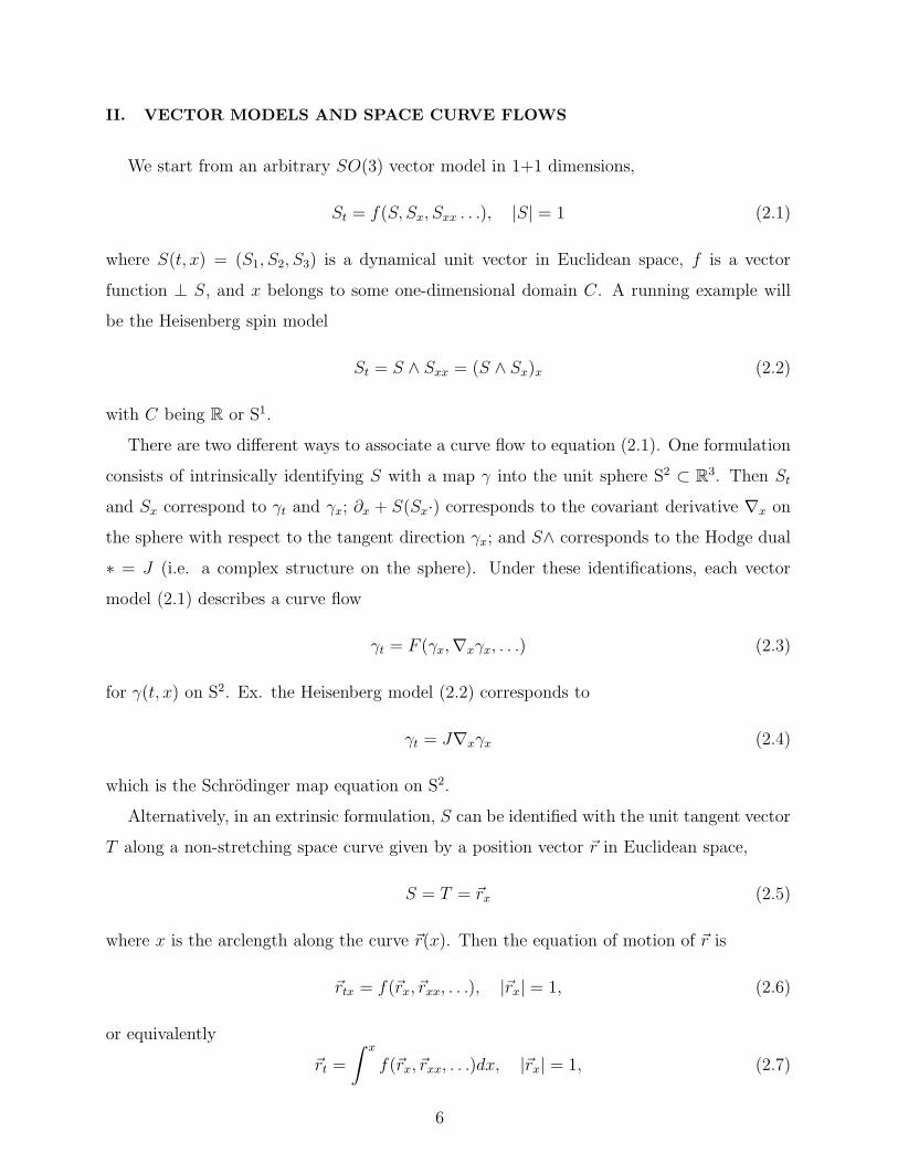
II. VECTOR MODELS AND SPACE CURVE FLOWS

We start from an arbitrary SO(3) vector model in 1+1 dimensions,

St = f(S, Sx, Sxx . . .), |S| = 1 (2.1)

where S(t, x) = (S1, S2, S3) is a dynamical unit vector in Euclidean space, f is a vector

function ⊥ S, and x belongs to some one-dimensional domain C. A running example will

be the Heisenberg spin model

St = S ∧ Sxx = (S ∧ Sx)x (2.2)

with C being R or S1.

There are two different ways to associate a curve flow to equation (2.1). One formulation

consists of intrinsically identifying S with a map γ into the unit sphere S2 ⊂ R3. Then St

and Sx correspond to γt and γx; ∂x + S(Sx·) corresponds to the covariant derivative ∇x on

the sphere with respect to the tangent direction γx; and S∧ corresponds to the Hodge dual

∗ = J (i.e. a complex structure on the sphere). Under these identifications, each vector

model (2.1) describes a curve flow

γt = F (γx,∇xγx, . . .) (2.3)

for γ(t, x) on S2. Ex. the Heisenberg model (2.2) corresponds to

γt = J∇xγx (2.4)

which is the Schrodinger map equation on S2.

Alternatively, in an extrinsic formulation, S can be identified with the unit tangent vector

T along a non-stretching space curve given by a position vector ~r in Euclidean space,

S = T = ~rx (2.5)

where x is the arclength along the curve ~r(x). Then the equation of motion of ~r is

~rtx = f(~rx, ~rxx, . . .), |~rx| = 1, (2.6)

or equivalently

~rt =

∫ x

f(~rx, ~rxx, . . .)dx, |~rx| = 1, (2.7)

6

under which the arclength of the curve is preserved, i.e.∫C|~rx|dx = ℓ is a constant of the

motion. Ex. the Heisenberg model (2.2) corresponds to

~rt = ~rx ∧ ~rxx (2.8)

with |~rx| = 1. This is the equation of motion of a non-stretching vortex filament studied by

Hasimoto [13].

To proceed we first introduce a Frenet frame E along ~r(x). It is expressed in matrix

column notation by

E =

T

N

B

(2.9)

where

T = ~rx, N = |Tx|−1Tx = |~rxx|−1~rxx, B = T ∧N = |~rxx|−1~rx ∧ ~rxx. (2.10)

Here N is the unit normal and B is the unit bi-normal of the space curve ~r(x). Note we

have the relations

S = T, Sx = κN, S ∧ Sx = κB, (2.11)

where

κ = Tx ·N = |Sx| (2.12)

is the curvature of ~r(x), and

τ = Nx · B = |Sx|−2Sxx · (S ∧ Sx) (2.13)

is the torsion of ~r(x). The Serret-Frenet equations of this frame (2.9) are given by

Ex = KE (2.14)

with

K =

0 κ 0

−κ 0 τ

0 −τ 0

∈ so(3). (2.15)

From the equation of motion (2.1) for S we obtain the frame evolution equation

Et = AE, A =

0 a2 a3

−a2 0 a1

−a3 −a1 0

∈ so(3) (2.16)

7

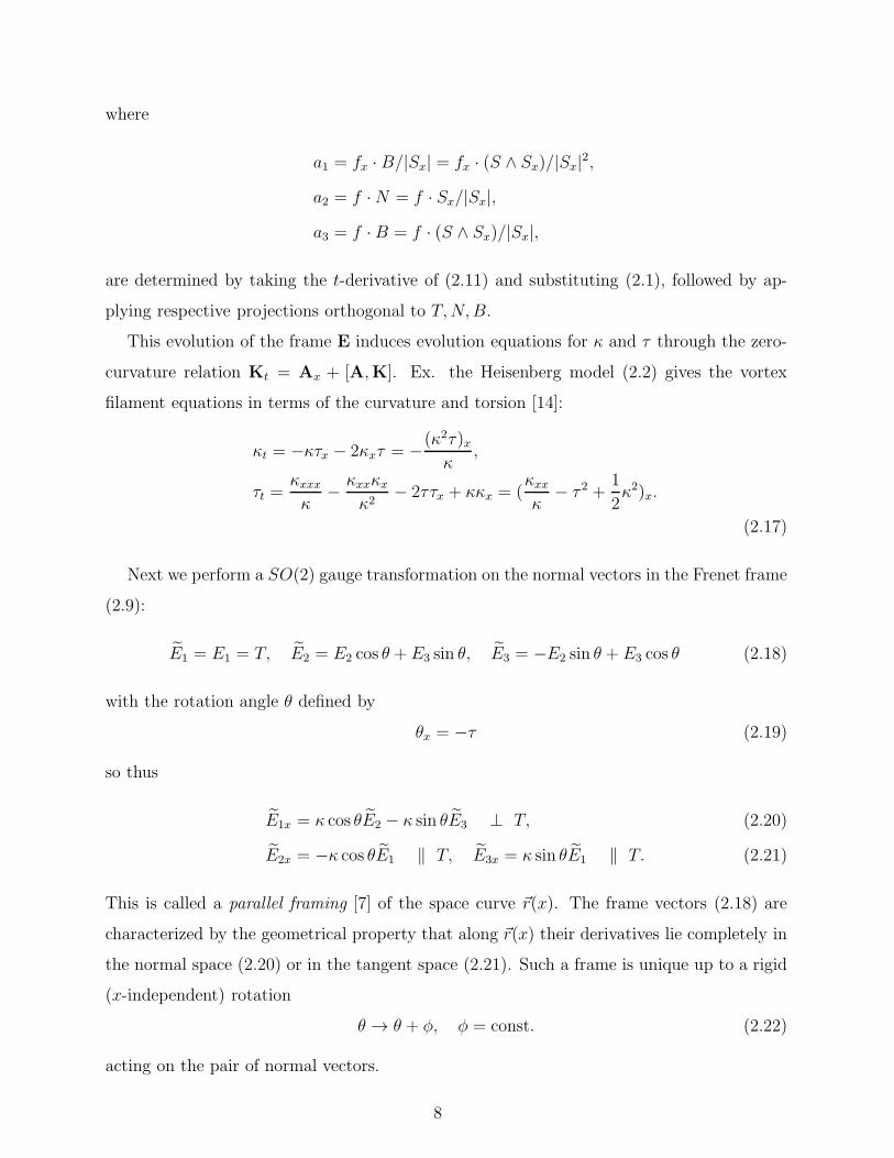
where

a1 = fx · B/|Sx| = fx · (S ∧ Sx)/|Sx|2,

a2 = f ·N = f · Sx/|Sx|,

a3 = f ·B = f · (S ∧ Sx)/|Sx|,

are determined by taking the t-derivative of (2.11) and substituting (2.1), followed by ap-

plying respective projections orthogonal to T,N,B.

This evolution of the frame E induces evolution equations for κ and τ through the zero-

curvature relation Kt = Ax + [A,K]. Ex. the Heisenberg model (2.2) gives the vortex

filament equations in terms of the curvature and torsion [14]:

κt = −κτx − 2κxτ = −(κ2τ)xκ

,

τt =κxxxκ

− κxxκxκ2

− 2ττx + κκx = (κxxκ

− τ 2 +1

2κ2)x.

(2.17)

Next we perform a SO(2) gauge transformation on the normal vectors in the Frenet frame

(2.9):

E1 = E1 = T, E2 = E2 cos θ + E3 sin θ, E3 = −E2 sin θ + E3 cos θ (2.18)

with the rotation angle θ defined by

θx = −τ (2.19)

so thus

E1x = κ cos θE2 − κ sin θE3 ⊥ T, (2.20)

E2x = −κ cos θE1 ‖ T, E3x = κ sin θE1 ‖ T. (2.21)

This is called a parallel framing [7] of the space curve ~r(x). The frame vectors (2.18) are

characterized by the geometrical property that along ~r(x) their derivatives lie completely in

the normal space (2.20) or in the tangent space (2.21). Such a frame is unique up to a rigid

(x-independent) rotation

θ → θ + φ, φ = const. (2.22)

acting on the pair of normal vectors.

8

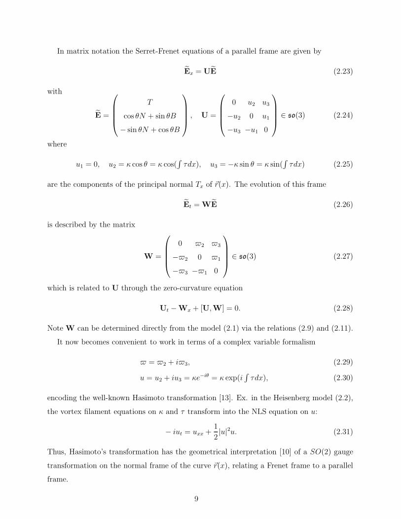
In matrix notation the Serret-Frenet equations of a parallel frame are given by

Ex = UE (2.23)

with

E =

T

cos θN + sin θB

− sin θN + cos θB

, U =

0 u2 u3

−u2 0 u1

−u3 −u1 0

∈ so(3) (2.24)

where

u1 = 0, u2 = κ cos θ = κ cos(∫τdx), u3 = −κ sin θ = κ sin(

∫τdx) (2.25)

are the components of the principal normal Tx of ~r(x). The evolution of this frame

Et = WE (2.26)

is described by the matrix

W =

0 2 3

−2 0 1

−3 −1 0

∈ so(3) (2.27)

which is related to U through the zero-curvature equation

Ut −Wx + [U,W] = 0. (2.28)

Note W can be determined directly from the model (2.1) via the relations (2.9) and (2.11).

It now becomes convenient to work in terms of a complex variable formalism

= 2 + i3, (2.29)

u = u2 + iu3 = κe−iθ = κ exp(i∫τdx), (2.30)

encoding the well-known Hasimoto transformation [13]. Ex. in the Heisenberg model (2.2),

the vortex filament equations on κ and τ transform into the NLS equation on u:

− iut = uxx +1

2|u|2u. (2.31)

Thus, Hasimoto’s transformation has the geometrical interpretation [10] of a SO(2) gauge

transformation on the normal frame of the curve ~r(x), relating a Frenet frame to a parallel

frame.

9

Remark: Since the form (2.25) of a parallel frame is preserved by SO(2) rotations

(2.22), the complex scalar variable (2.30) given by the Hasimoto transformation is uniquely

determined by the curve ~r(x) up to rigid phase rotations u → e−iφu, depending on an

arbitrary constant φ. Therefore, u has the geometrical meaning of a covariant of the curve

[5] relative to the group SO(2) ≃ U(1), while |u| = κ and (arg u)x = τ are invariants of the

curve.

III. BI-HAMILTONIAN FLOWS AND OPERATORS

For a general vector model (2.1) the zero-curvature equation (2.28) gives an evolution

equation on u,

ut = x − i1u, (3.1)

plus an auxiliary equation relating 1 to u,

1x = Im( ¯ u). (3.2)

From (3.2) we can eliminate 1 = D−1x Im( ¯ u) in terms of u and , and then we see (3.1)

yields

ut = Dx − iuD−1x Im( ¯ u) = H() (3.3)

where is determined from (2.1) via the frame evolution equation (2.26).

Proposition 1.

H = Dx − iuD−1x Im(uC) (3.4)

is a Hamiltonian operator with respect to the flow variable u(t, x), whence the evolution

equation (3.3) has a Hamiltonian structure

ut = H(δH/δu) (3.5)

iff

= δH/δu (3.6)

holds for some Hamiltonian

H =

∫

C

H(x, u, u, ux, ux, uxx, uxx, . . .)dx. (3.7)

10

Here C is the complex conjugation operator, and C = R or S1 is the domain of x. In the

present setting, an operator D is Hamiltonian if it defines an associated Poisson bracket

{H,G} =

∫

C

Re(D(δH/δu)δG/δu)dx (3.8)

obeying skew-symmetry {H,G} = −{G,H} and the Jacobi identity {F, {H,G}}+cyclic = 0,

for all real-valued functionals F, G, H on the x-jet space of the flow variable u.

Proposition 2. (i) The Hamiltonian operator H is invariant with respect to U(1) phase

rotations eiλHe−iλ = H|u→eiλu. (ii) A second Hamiltonian operator is given by

I = −i (3.9)

which is similarly U(1)-invariant, eiλIe−iλ = I. (iii) The operatorsH and I are a compatible

Hamiltonian pair (i.e. every linear combination is again a Hamiltonian operator), and their

compositions define U(1)-invariant hereditary recursion operators

R = HI−1 = i(Dx + uD−1x Re(uC)), R∗ = I−1H = iDx − uD−1

x Re(iuC). (3.10)

(iv) Composition of R and H yields a third U(1)-invariant Hamiltonian operator

E = RH = iD2x +Dx(uD

−1x Im(uC)) + iuD−1

x Re(uDxC) (3.11)

= iD2x + i|u|2 + uxD

−1x Im(uC)− iuD−1

x Re(uxC)

satisfying eiλEe−iλ = E|u→eiλu. In particular, E , H, I form a compatible Hamiltonian triple.

These Propositions are a special case of group-invariant bi-Hamiltonian operators derived

from non-stretching curve flows in constant-curvature spaces and general symmetric spaces

in recent work [3–5, 24]. Moreover, in the present complex variable formalism, Proposition 2

provides a substantial simplification of some main results in [17] on Hamiltonian operators

connected with non-stretching curve flows in Euclidean space.

Because phase rotation on u is a symmetry of both H and I, the recursion operator Rgenerates a hierarchy of commuting Hamiltonian vector fields given by

i(n)∂/∂u = Rn(iu)∂/∂u, n = 0, 1, 2, . . . (3.12)

where

(n) = δH(n)/δu = R∗n(u), n = 0, 1, 2, . . . (3.13)

11

are Hamiltonian derivatives, starting with

(0) = u, H(0) = uu = |u|2 (3.14)

which corresponds to phase-rotation iu∂/∂u. Next in the hierarchy comes

(1) = iux, H(1) =i

2(uux − uux) = Im(uxu), (3.15)

followed by

(2) = −(uxx +1

2|u|2u), H(2) = |ux|2 −

1

4|u|4, (3.16)

corresponding to respective Hamiltonian vector fields −ux∂/∂u which is x-translation and

−i(uxx + 12|u|2u)∂/∂u which is of NLS form.

Through Propositions 1 and 2, this hierarchy produces integrable evolution equations

on u(t, x) with a tri-Hamiltonian structure. An explicit formulation of this result has not

appeared previously in the literature.

Theorem 1. There is a hierarchy of integrable bi-Hamiltonian flows on u(t, x) given by

ut = H(δH(n)/δu) = I(δH(n+1)/δu), n = 0, 1, 2, . . . (3.17)

(called the +n flow) in terms of Hamiltonians H(n) =∫CH(n)dx where

H(n) =2

1 + nD−1x Im(u(iH)n+1u) n = 0, 1, 2, . . . (3.18)

are local Hamiltonian densities. Moreover, all the flows for n 6= 0 have a tri-Hamiltonian

structure

ut = E(δH(n−1)/δu), n = 1, 2, . . . . (3.19)

Remarks: Each flow n = 0,+1,+2, . . . in the hierarchy is U(1)-invariant under the

phase rotation u→ eiλu and has scaling weight t→ λ1+nt under the NLS scaling symmetry

x→ λx, u → λ−1u, where the scaling weight of H(n) is −2−n. Additionally, these flows on

u(t, x) each admit constants of motion (under suitable boundary conditions)

Dt

∫

C

|u|2dx = 0, Dt

∫

C

iuux dx = 0, Dt

∫

C

|ux|2 −1

4|u|4dx = 0, . . . (3.20)

and symmetries

− ux∂/∂u, −i(uxx +1

2|u|2u)∂/∂u, (uxxx +

3

2|u|2u)∂/∂u, . . . (3.21)

12

respectively comprising all of the Hamiltonians (3.18) in the hierarchy and all of the corre-

sponding Hamiltonian vector fields (3.12).

At the bottom of the hierarchy, the 0 flow is given by a linear traveling wave equation

ut = ux, and next the +1 flow produces the NLS equation (2.31). The +2 flow yields the

complex mKdV equation

− ut = uxxx +3

2|u|2u (3.22)

which corresponds to an mKdV analog of the vortex filament equations,

− κt = (κxx +1

2κ3)x −

3

2

(τ 2κ2)xκ

= κxxx +3

2(κ2 − 2τ 2)κx − 3κττx, (3.23)

−τt = (τxx + 3(τκx)xκ

+3

2τκ2 − τ 3)x (3.24)

= τxxx + 3τxxκxκ

+ τx(6κxxκ

− 3κ2xκ2

− 3τ 2 +3

2κ2) + τ(3

κxxxκ

− 3κxxκxκ2

+ 3κκx),

as obtained through the Hasimoto transformation u = κ exp(−iθ).The evolution equations describing the 0,+1,+2, . . . flows on u each arise from geomet-

ric space curve flows corresponding to SO(3)-invariant vector models (2.1). To make this

correspondence explicit, it is convenient to introduce a complex frame notation

E‖ = E1 = T, E⊥ = E2 + iE3 = e−iθ(N + iB) (3.25)

satisfying

E‖ ∧ E⊥ = −iE⊥ = E3 − iE2 = e−iθ(B − iN) (3.26)

and

E‖ · E‖ = 1, E⊥ · E⊥ = 2, E‖ ·E⊥ = 0 = E⊥ · E⊥. (3.27)

The Frenet equations (2.14) become

E‖x = Re(uE⊥), E⊥

x = −uE‖, (3.28)

while from (2.27), (2.29), (3.2), the evolution of the frame is given by the equations

E‖t = Re( ¯E⊥), E⊥

t = iD−1x Im(u)E⊥ −E‖. (3.29)

Then any flow belonging to the general class

= (u, u, ux, ux, uxx, uxx, . . .) (3.30)

13

will determine a vector model (2.1) via

S = E‖, f = Re( ¯E⊥), (3.31)

where f is expressed in terms of S, Sx, Sxx, etc. through the Frenet equations (2.23)–(2.24).

Ex. 1: The +1 flow = iux yields

E‖t = −Re(iuxE

⊥). (3.32)

By rewriting

uxE⊥ = (uE⊥)x + uuE‖

we obtain

Re(iuE⊥) = −E‖ ∧ Re(uE⊥) = −E‖ ∧ E‖x,

Re(iuuE‖) = Re(i|u|2)E‖ = 0,

and hence

E‖t = (E‖ ∧ E‖

x)x. (3.33)

The identifications (3.31) then directly give the SO(3) Heisenberg model (2.2), which cor-

responds to the non-stretching space curve flow (2.17) or equivalently

~rt = κB, |~rx| = 1 (3.34)

expressed as a geometric flow.

Ex. 2: The +2 flow = −(uxx +12|u|2u) yields

−E‖t = Re((uxx +

1

2|u|2u)E⊥) = Re(uxxE

⊥) +1

2|u|2E‖

x. (3.35)

Here we can rewrite the first term as

Re(uxxE⊥) = Re(uE⊥)xx − Re(uE⊥

x )x − Re(uxE⊥x ) = E‖

xxx + (|u|2E‖)x +1

2(uu)xE

‖,

with |u|2 = |E‖x|2, and thus

− E‖t = E‖

xxx +3

2(|E‖

x|2E‖)x. (3.36)

Hence, E‖ = S gives

− St = Sxxx +3

2(|Sx|2S)x (3.37)

14

which can be viewed as an SO(3) mKdV model. The corresponding non-stretching space

curve flow looks like

− ~rt = ~rxxx +3

2|~rxx|2~rx, |~rx| = 1. (3.38)

This describes a geometric flow [16]

− ~rt =1

2κ2T + κxN + κτB, |~rx| = 1 (3.39)

which is equivalent to the evolution (3.23) and (3.24) on the curvature and torsion of ~r(x).

Remark: A different geometric derivation of the mKdV model (3.37) appears in work [2]

on non-stretching flows of curves in three-dimensional manifolds with constant curvature,

i.e. S3, H3, R3, where the spin vector S is identified with the components of the unit

tangent vector in a moving frame defined by parallel transport along the curve. The mKdV

model also has been derived in [11] as a higher-order symmetry of the Heisenberg model by

non-geometric methods.

All of these SO(3) vector models describe dynamical maps γ on the unit sphere S2 ⊂ R3

by means of the identifications:

St ↔ γt, Sx ↔ γx, ∂x + S(Sx·) ↔ ∇x, S∧ ↔ J = ∗ (3.40)

and thus

∇xγx ↔ Sxx + |Sx|2S, ∇2xγx ↔ Sxxx + |Sx|2Sx +

3

2(|Sx|2)xS, (3.41)

Jγx ↔ S ∧ Sx, J∇xγx ↔ S ∧ Sxx, (3.42)

g(γx, γx) = |γx|2g ↔ |Sx|2 = Sx · Sx (3.43)

where g denotes the Riemannian metric on the sphere S2 (given by restricting the Euclidean

inner product in R3 to the tangent space of S2 ⊂ R

3).

In particular, the SO(3) Heisenberg model yields the Schrodinger map equation (2.4) on

S2, while the SO(3) mKdV model (3.37) is identified with

− γt = ∇2xγx +

1

2|γx|2gγx (3.44)

which is a mKdV map equation on S2 (i.e. a dynamical map version of the potential mKdV

equation).

Thus, Theorem 1 provides a geometric realization of the hierarchies of integrable vector

models and dynamical maps containing the Heisenberg model and the Schrodinger map as

well as their mKdV counterparts.

15

IV. GEOMETRIC HIERARCHY OF INTEGRABLE VECTOR MODELS AND

DYNAMICAL MAPS

In general, any non-stretching space curve flow (2.7) can be written in terms of a Frenet

frame (2.9) by an equation of motion of the form

~rt = aT + bN + cB (4.1)

such that

Dxa = κb. (4.2)

This relation between the tangential and normal components of the motion arises due to the

non-stretching property

|~rx| = 1 (4.3)

by which the motion preserves the local arclength ds = |~rx|dx of the space curve if (and

only if) ~rx · ~rtx = 0. As a consequence, through the Serret-Frenet equations (2.14)–(2.15),

the tangent vector T = ~rx along the space curve obeys the equation of motion

Tt = f1N + f2B = f ⊥ T (4.4)

given by a linear combination of the normal and bi-normal vectors with coefficients

f1 = Dxb− τc + κa, f2 = Dxc+ τb. (4.5)

Now we consider a Hasimoto transformation (2.18)–(2.19) from the Frenet frame (2.9) to

a parallel frame (3.25). The equation of motion (4.1) on ~r takes the form

~rt = h‖E‖ + Re(h⊥E

⊥) = h‖T + Re(h⊥eiθ)N + Im(h⊥e

iθ)B (4.6)

in terms of the tangential and normal components given by

h⊥ = (b+ ic)e−iθ, h‖ = a, (4.7)

with these components satisfying the relation (4.2) given by

Dxh‖ = Re(uh⊥) (4.8)

where u = κe−iθ. Correspondingly, from the Frenet equations (3.28) of the parallel frame,

the equation of motion (4.4) for the tangent vector T = ~rx has the form

Tt = Re( ¯E⊥) = Re(eiθ)N + Im(eiθ)B (4.9)

16

in terms of

= Dxh⊥ + h‖u (4.10)

which encodes the normal and bi-normal components

f1 + if2 = eiθ. (4.11)

The evolution of T is thus specified by the variable , while the underlying evolution

of ~r is specified in terms of the variable h⊥, with h‖ given by the non-stretching condition

(4.8). From equation (4.10) these variables are related by

= Dxh⊥ + uD−1x Re(uh⊥) = J (h⊥). (4.12)

The operator here

J = Dx + uD−1x Re(uC) (4.13)

is related to the Hamiltonian operator I = −i by the properties

−J = R∗I−1 = I−1R and − J −1 = R−1I = IR∗−1, (4.14)

where R and R∗ are the recursion operators (3.10). Consequently, J −1 is a formal Hamil-

tonian operator compatible with I.

Proposition 3. The evolution (4.1) of a non-stretching space curve ~r(x) can be expressed

in terms of a geometrical variable that determines the corresponding evolution (4.4) of the

tangent vector T = ~rx through the relation Tt = (~rt)x. In particular,

h⊥ = J −1() = R−1(i) = iR∗−1() (4.15)

yields the normal components of the evolution vector ~rt in a parallel frame, where repre-

sents the frame components of Tt. The curvature κ and torsion τ of ~r(x) correspondingly

have the evolution

κt = Dxf1 − τ f2 = Re(eiθDx) (4.16)

τt = Dx(κ−1Dxf2 + τκ−1f1) + κf2 = Dx(κ

−1Im(eiθDx)) + κIm(eiθ) (4.17)

which can be expressed in terms of the Frenet frame coefficients a, b, c of ~rt through the

relations (4.5).

17

Conditions will now be stated within the general class of flows (3.30) on u such that

the various evolutions (4.16)–(4.17), (4.9), (4.6), (4.4), (4.1), and (3.5)–(3.6) each define a

geometric flow.

Theorem 2. For a non-stretching flow of a space curve ~r(x) in R3, the following conditions

are equivalent:

(i) Its tangent vector T = ~rx = S obeys a SO(3)-invariant vector model iff f1 and f2 are

functions of scalar invariants formed out of S and its x derivatives (modulo differential

consequences of S · S = 1), i.e.

f1+if2 = f(Sx·Sx, Sx·Sxx, Sxx·Sxx, . . . , Sxx·(S∧Sx), Sxxx·(S∧Sx), Sxxx·(S∧Sxx), . . .). (4.18)

(ii) Its principal normal component u = Tx · E⊥ in a parallel frame (3.25) satisfies a U(1)-

invariant evolution equation iff is an equivariant function of u, u, and x derivatives of

u and u, under the action of a rigid (x-independent) U(1) rotation group u → e−iφu (with

φ =const.), i.e.

= uf(|u|, |u|x, |u|xx, . . . , (arg u)x, (arg u)xx, . . .). (4.19)

(iii) Its curvature κ and torsion τ satisfy geometric evolution equations in terms of invariants

and differential invariants of ~r(x) iff eiθ is a function of κ, τ , and their x derivatives, i.e.

= e−iθκf(κ, κx, κxx, . . . , τ, τx, τxx, . . .). (4.20)

(iv) Its equation of motion is invariant under the Euclidean isometry group SO(3)⋊ R3 iff

a, b, c are scalar functions of the curvature κ, torsion τ , and their x-derivatives, subject to

the non-stretching condition (4.2).

The proof of this proposition amounts to enumerating the Euclidean (differential) invari-

ants of a space curve ~r(x) with an arclength parameterization x, as shown in appendix A.

We are now able to derive the entire hierarchy of SO(3)-invariant vector models and

geometric space curve motions that correspond to all of the U(1)-invariant flows on u in

Theorem 1.

From equation (4.9) combined with the hierarchy (3.6), the evolution of the spin vector

S = T = ~rx can be written as

St = Re(E⊥R∗n(u)), n = 0, 1, 2, . . . (4.21)

18

as generated via the recursion operator R∗ = iDx− uD−1x Re(iuC). The main step is now to

establish the operator identity

Re(E⊥R∗) = SRe(E⊥C) (4.22)

where S is a spin vector operator corresponding to R∗, and Re(E⊥C) is the operator that

produces a vector f in the perp space of S in R3 when applied to the components of f with

respect to E⊥ (i.e. f = Re(E⊥Cf) if f · S = 0, where f = f · E⊥). Through the Frenet

equations (3.28) and the orthonormality relations (3.27) on E⊥ and E‖, we straightforwardly

find

Re(E⊥u) = E‖x = Sx (4.23)

and

Re(E⊥iDxf) = E‖ ∧ Re(E⊥Dxf) = S ∧DxRe(E⊥Cf) = S ∧Dxf

D−1x Re(iuCf) = D−1

x Re((E‖ ∧ E‖x) · E⊥Cf) = D−1

x Re((S ∧ Sx) · f)

for any vector f(x), orthogonal to S in R3, with components f(x) = E⊥ · f(x). Hence, this

yields the vector operator

S = S ∧Dx − SxD−1x (S ∧ Sx)· (4.24)

Theorem 3. The bi-Hamiltonian flows (3.17) on u(t, x) correspond to a hierarchy of inte-

grable SO(3)-invariant vector models

St =(S ∧Dx − SxD

−1x (S ∧ Sx)·

)nSx = f (n), n = 0, 1, 2, . . . (4.25)

generated by the recursion operator (4.24). These models have the equivalent geometrical

formulation

γt =(J∇x − γxD

−1x g(Jγx, )

)nγx = F (n), n = 0, 1, 2, . . . (4.26)

expressed as dynamical maps γ(t, x) into the 2-sphere S2 ⊂ R3. Moreover, the Hamiltonians

(3.18) for all the flows on u(t, x) correspond to a set of constants of motion H(0) =∫CH(0)dx,

H(1) =∫CH(1)dx, H(2) =

∫CH(2)dx, etc. for each vector model (4.25) and each dynamical

map equation (4.26). This entire set has the explicit form given by the densities (modulo

total x-derivatives)

(1 + n)H(n) = D−1x (Sx ·Dxf

(n)) = D−1x g(γx,∇xF

(n)), n = 0, 1, 2, . . . (4.27)

19

which are scalar polynomials formed out of SO(3)-invariant wedge products and dot products

of S, Sx, Sxx, . . . in terms of the equations of motion for S(t, x), or equivalently, scalar inner

products of γx, Jγx,∇xγx, J∇xγx, . . . formed in terms of the equations of motion for γ(t, x).

The vector models (4.25) have been derived previously in [6] by non-geometric methods

(based on a Lax pair representation). As one new result, Theorem 3 derives the equiva-

lent dynamical map equations (4.26), along with their recursion operator, and provides an

explicit expression for the constants of motion for all of these integrable generalizations of

the Heisenberg spin model (2.2) and the mKdV spin model (3.37). In particular, from the

hierarchy (4.25), higher-derivative versions of the Heisenberg spin model n = 1 as given

by n = 3, 5, . . . are seen to describe higher-derivative Schrodinger maps; similarly, higher-

derivative versions of the mKdV spin model n = 2 as given by n = 4, 6, . . . are found to

describe higher-derivative mKdV maps.

Ex: n = 3 and n = 4 respectively yield a 4th order Heisenberg vector model

St = S ∧ Sxxxx +5

2(|Sx|2S ∧ Sx)x (4.28)

and a 5th order mKdV vector model

− St = Sxxxxx −5

2(|Sxx|2S + |Sx|2Sx −

7

4|Sx|4S)x +

5

2(|Sx|2S)xxx (4.29)

which are described geometrically by a 4th order Schrodinger map equation

− γt = J∇3xγx +

1

2∇x(|γx|2gJγx)−

1

2g(Jγx,∇xγx)γx (4.30)

and a 5th order mKdV map equation

γt = ∇4xγx +

3

4(|γx|2g)x∇xγx + (

5

4(|γx|2g)xx −

3

2|∇xγx|2g +

3

8|γx|4g)γx. (4.31)

Remark: The equations of motion of these dynamical maps γ(t, x) do not locally preserve

the arclength ds = |γx|gdx in the x direction along γ on S2, namely |γx|g has a nontrivial

time evolution for any of the dynamical map equations (4.26), and additionally, the total

arclength∫C|γx|gdx is time dependent.

The spin vector recursion operator (4.24) has the factorization

S = (Dx + SSx · +SxD−1x Sx· )(S∧ ) (4.32)

20

where, as shown by the results in [6], the operatorsDx+SSx·+SxD−1x Sx· and (S∧ )−1 = −S∧

constitute a compatible Hamiltonian pair with respect to the spin vector variable S(t, x). By

comparison, using the present geometric framework, we now directly derive the explicit bi-

Hamiltonian structure of the hierarchy of vector models (4.25) through the bi-Hamiltonian

flow equation (3.17) on u(t, x) in Theorem 1.

The starting point is the variational identity

δH(n) ≡ δS · (δH(n)/δS) ≡ 2Re( ¯ (n)δu) (4.33)

holding modulo total x-derivatives and modulo (differential consequences of) S · δS = 0,

with the Hamiltonian densities given in the equivalent forms (3.18) and (4.27), and with

(n) given by the hierarchy (3.13) generated through the recursion operator R∗. To begin

we derive an explicit expression for δu in terms of δS = δE‖ by taking the Frechet derivative

of the Frenet equation (3.28) for the normal vectors in a parallel frame with respect to u:

DxδE⊥ = −δuE‖ − uδE‖. (4.34)

The E⊥ component of (4.34) gives

Dx(E⊥ · δE⊥) = −uE⊥ · δE‖ − uE‖ · δE⊥ = −2iRe(iuE⊥ · δE‖)

via E‖ · δE⊥ = −E⊥ · δE‖ due to the orthogonality of E⊥, E‖. Similarly, the E‖ component

of (4.34) yields

δu = Dx(E⊥ · δE‖) +

1

2uE⊥ · δE⊥.

Combining these two expressions, we obtain

δu = Dx(E⊥ · δE‖)− iuD−1

x Re(iuE⊥ · δE‖) (4.35)

whence

Re( ¯ (n)δu) = Re( ¯ (n)Dx(E⊥ · δE‖)) + Im( ¯ (n)u)D−1

x Re(iuE⊥ · δE‖). (4.36)

Integration by parts on both terms in (4.36) then yields

Re( ¯ (n)δu) = −Re(E⊥ · δE‖Dx ¯(n))− Re(iuE⊥ · δE‖D−1

x Im( ¯ (n)u))

≡ −δE‖ ·Re(E⊥H((n))) (4.37)

21

modulo total x-derivatives. Next, after use of the relations iR∗ = −H and iE⊥ = E‖ ∧ E⊥

which follow from (3.10) and (3.26), we get

Re( ¯ (n)δu) ≡ δE‖ · (E‖ ∧ Re(E⊥(n+1))). (4.38)

Hence, equating (4.38) and (4.33) yields

δS · (δH(n)/δS − 2S ∧ Re(E⊥(n+1))) ≡ 0

from which we obtain the variational relation

− S ∧ (δH(n)/δS) = 2Re(E⊥(n+1)) = 2Re(E⊥R∗n+1(u)) = 2f (n+1) (4.39)

where the final equality comes from the equation of motion (4.21) combined with the hier-

archy (4.25). This result (4.39), together with the factorization of the recursion operator

(4.32), leads to the following Hamiltonian structure.

Theorem 4. In terms of the Hamiltonian densities (4.27), the hierarchy of vector models

(4.25) for S(t, x) has two Hamiltonian structures

St = −S ∧ (δH(n−1)/δS) = f (n), n = 1, 2, . . . (4.40)

and, for n 6= 1,

St = Dx(δH(n−2)/δS + SD−1

x (Sx · δH(n−2)/δS)) = f (n), n = 2, 3, . . . (4.41)

where

S ∧ and Dx + SSx · +SxD−1x Sx· (4.42)

are a compatible pair of Hamiltonian operators. Correspondingly, the hierarchy of dynamical

maps (4.26) on γ(t, x) has the Hamiltonian structures

γt = −J(δH(n−1)/δγ) = F (n), n = 1, 2, . . . (4.43)

= ∇x(δH(n−2)/δγ) + γxD

−1x g(γx, δH

(n−2)/δγ), n = 2, 3, . . . (4.44)

in terms of the compatible Hamiltonian operators

J and ∇x + γxD−1x g(γx, ) (4.45)

as given by the geometrical identifications (3.40). Moreover, these bi-Hamiltonian pairs

(4.42) and (4.45) are geometrically equivalent to the pair of compatible symplectic (inverse

Hamiltonian) operators −I−1 and J = −R∗I−1 with respect to the flow variable u(t, x) in

the hierarchy (3.17)–(3.18) (cf. Theorems 1 and 3).

22

These results provide an explicit geometrical formulation of the abstract symplectic struc-

ture given in [28] for the Schrodinger map equation (2.4), i.e. (n = 1)

γt = J∇xγx = −J(δH(0)/δγ), H(0) =1

2g(γx, γx), (4.46)

and its higher-order generalizations (n = 3, 5, . . .); the Hamiltonian structure of the mKdV

map, i.e. (n = 2)

γt = −∇2xγx −

1

2|γx|2gγx = ∇x(δH

(0)/δγ) + γxD−1x g(γx, δH

(0)/δγ) (4.47)

= −J(δH(1)/δγ), H(1) = −1

2g(∇xγx, Jγx), (4.48)

and its higher-order generalizations (n = 4, 6, . . .) has not appeared previously in the litera-

ture. Note the n = 1 and n = 2 vector models respectively yield the well-known Hamiltonian

structure of the Heisenberg spin model (2.2),

St = S ∧ Sxx = −S ∧ (δH(0)/δS), H(0) =1

2|Sx|2, (4.49)

and the mKdV spin model (3.37),

St = −Sxxx −3

2(|Sx|2S)x = Dx(δH

(0)/δS + SD−1x (Sx · δH(0)/δS)) (4.50)

= −S ∧ (δH(1)/δS), H(1) =1

2Sx · (S ∧ Sxx). (4.51)

Remark: There is a second Hamiltonian structure for both the Schrodinger map equation

and the Heisenberg spin model. This structure, in contrast to the first Hamiltonian structure

(4.46) and (4.49), turns out to involve a non-polynomial Hamiltonian density defined as

follows. Let ξ(γ) be a vector field on S2 such that its divergence is constant at all points

γ ∈ S2. (This property geometrically characterizes ξ(γ) as a homothetic vector with respect

to the metric-normalized volume form ǫg on S2, i.e. Lξǫg = cǫg for some constant c 6= 0.)

Then the Hamiltonian density given by

H(−1) = g(ξ(γ), J∇γx), divgξ(γ) = 1 (4.52)

can be shown to satisfy (see Appendix B)

δH(−1) ≡ g(δγ, J∇γx) (4.53)

modulo total x-derivatives, so thus

γt = ∇x(δH(−1)/δγ) + γxD

−1x g(γx, δH

(−1)/δγ) = ∇x(Jγx) (4.54)

23

yields a second Hamiltonian structure for the Schrodinger map (2.4). The corresponding

second Hamiltonian structure for the Heisenberg spin model (2.2) is given by

St = Dx(δH(−1)/δS +SD−1

x (Sx · δH(−1)/δS)) = (S ∧Sx)x, H(−1) = ξ(S) · (S ∧Sx) (4.55)

in terms of a vector function ξ(S) such that

S · ξ(S) = 0, ∂⊥S · ξ(S) = 1, (4.56)

where the operator ∂⊥S = ∂S − S(S · ∂S) is the orthogonal projection of a gradient with

respect to the components of S. From the properties

S · ∂⊥S = 0, ∂⊥S (S · S) = 0, (4.57)

the Hamiltonian density can be shown to satisfy

δH(−1) ≡ δS · (S ∧ Sx) (4.58)

modulo total x-derivatives (see Appendix C). Thus, both the Heisenberg spin model and

the Schrodinger map equation are Hamiltonian equations of motion with respect to the

corresponding bi-Hamiltonian pairs (4.42) and (4.45).

To conclude, a counterpart of Theorem 3 will now be stated for the underlying space

curve motions on ~r.

Theorem 5. The SO(3)-invariant vector models (4.25) on S(t, x) correspond to a hierarchy

of integrable flows of non-stretching space curves

~rt = a(n−1)T + b(n−1)N + c(n−1)B, |~rx| = 1, n = 1, 2, . . . (4.59)

with geometric coefficients

c(n) = Re(Qnκ), b(n) = −Im(Qnκ), (4.60)

a(n) = −D−1x (κIm(Qnκ)) (4.61)

given in terms of the recursion operator

Q = iDx − τ − κD−1x (κIm) = eiθR∗e−iθ, (4.62)

where κ, τ are the curvature and torsion of ~r. The tangential coefficients (4.61) yield a set

of non-trivial constants of motion∫Ca(1)dx = −

∫C

12κ2dx,

∫Ca(2)dx =

∫Cτκ2dx, etc. for

each curve flow (4.59) in the hierarchy (under suitable boundary conditions), where C = R

or S1 is the coordinate domain of x.

24

The equations of motion (4.59) arise from writing the flow equation (4.6) on ~r in terms

of the hierarchy (3.6) by means of the relation (4.15). This yields

a(n) = D−1x Re(iu(n−1)) = −D−1

x Im(u(n−1)), (4.63)

b(n) = Re(ieiθ(n−1)) = −Im(eiθ(n−1)), (4.64)

c(n) = Im(ieiθ(n−1)) = Re(eiθ(n−1)). (4.65)

The geometric form (4.60)–(4.61) for these coefficients is then obtained through the identity

eiθ(n−1) = eiθR∗n−1u = (eiθR∗e−iθ)n−1eiθu (4.66)

combined with the Hasimoto transformation

κ = eiθu, τ = −θx. (4.67)

V. SURFACES AND SPATIAL HAMILTONIAN CURVE FLOWS

The results in Theorem 1 for 1+1 flows can be generalized in a natural way to 2+1 flows

by considering surfaces ~r(x, y) that are foliated by space curves with a parallel framing in

R3. Here y will denote a coordinate assumed to be transverse to these curves, and x will

denote the arclength coordinate along the curves, so thus

|~rx| = 1. (5.1)

In this setting, a parallel frame consists of a triple of unit vectors whose derivatives along

each y = const. coordinate line on the surface ~r(x, y) lie completely in either the tangent

space or the normal plane of this line in R3. The explicit form of such a frame is given by

the vectors

E1 = T = ~rx, (5.2)

E2 = Re(e−iθ(N + iB)) = |~rxx|−1(cos θ ~rxx + sin θ ~rx ∧ ~rxx), (5.3)

E3 = Im(e−iθ(N + iB)) = |~rxx|−1(− sin θ ~rxx + cos θ ~rx ∧ ~rxx), (5.4)

with

θx = −|~rxx|−2(~rx ∧ ~rxx) · ~rxxx (5.5)

25

where T,N,B respectively denote the unit tangent vector, unit normal and bi-normal vectors

of the y = const. coordinate lines.

In matrix notation these frame vectors satisfy the Frenet equations

Ex = UE, Ey = VE (5.6)

given by

E =

E1

E2

E3

, U =

0 u2 u3

−u2 0 0

−u3 0 0

∈ so(3), V =

0 v2 v3

−v2 0 v1

−v3 −v1 0

∈ so(3), (5.7)

where

u2 + iu3 = u = (E2 + iE3) · E1x, v2 + iv3 = v = (E2 + iE3) · E1y (5.8)

are complex scalar variables, and

v1 =1

2(E3 + iE2) · (E2y + iE3y) = v1 (5.9)

is a real scalar variable. Note, similarly to the case of space curves, here we have

(E3 + iE2) · (E2x + iE3x) = 0 (5.10)

which characterizes E(x, y) as a parallel frame adapted to the foliation of the surface ~r(x, y)

by x-coordinate lines, i.e. E1x ⊥ T , E2x ‖ T , E3x ‖ T . From (5.5) we see this choice

of framing is geometrically unique up to rigid rotations that act on the normal vectors

(5.3)–(5.4):

θ → θ + φ, E2 + iE3 → exp(−iφ)(E2 + iE3), with φ =const. . (5.11)

Under such rotations, v1 is invariant, while u and v undergo a rigid phase rotation,

u→ e−iφu, v → e−iφv. (5.12)

To proceed we need to write down the tangent vectors of ~r(x, y) in terms of the parallel

framing,

~rx = E1, ~ry = q1E1 + q2E2 + q3E3. (5.13)

The respective projections of ~ry orthogonal and parallel to ~rx are given by the scalar variables

q2 + iq3 = q = (E2 + iE3) · ~ry, q1 = E1 · ~ry, (5.14)

26

where, under rigid rotations (5.11) on the normal vectors in the parallel frame, q1 is invariant

while q transforms by a rigid phase rotation,

q → e−iφq. (5.15)

Remark: Due to the transformation properties (5.12) and (5.15), the variables u, v, q

represent U(1)-covariants of ~r(x, y) as geometrically defined with respect to the x-coordinate

lines, where U(1) is the equivalence group of rigid rotations (5.11) that preserves the form

of the framing (5.2)–(5.5) for the surface ~r(x, y). These variables will be seen later (cf.

Propositions 7 and 8) to encode both the intrinsic and extrinsic surface geometry of ~r(x, y)

in R3.

We will now show that all surfaces ~r(x, y) with the x coordinate satisfying the non-

stretching property (5.1) have a natural geometrical interpretation as a spatial Hamiltonian

curve flow with respect the y coordinate. This interpretation arises directly from the struc-

ture equations satisfied by the parallel frame (5.2)–(5.4) and the tangent vectors (5.13)

adapted to these coordinates. Firstly, the frame connection matrices given in (5.7) obey the

zero-curvature condition Uy −Vx + [U,V] = 0, which yields the structure equations

uy − vx + iv1u = 0, v1x − Im(vu) = 0. (5.16)

Secondly, the frame expansions of the tangent vectors given by (5.13) obey the zero-torsion

condition (~rx)y = (~ry)x, leading to the structure equations

v − qx − q1u = 0, q1x − Re(qu) = 0. (5.17)

Proposition 4. Through the frame structure equations (5.16) and (5.17), the U(1)-

covariants u, v, q of ~r(x, y) are related by the Hamiltonian equations

uy = H(v), v = J (q), (5.18)

with J = −I−1R = −R∗I−1, where H = Dx − iuD−1x Im(uC) and I = −i are a pair of

compatible Hamiltonian operators with respect to u, and R = HI−1 = i(Dx + uD−1x Re(uC))

and R∗ = I−1H = iDx − uD−1x Re(iuC) are the associated recursion operators.

This leads to a main preliminary geometric result.

27

Lemma 1. Let u be an arbitrary complex-valued function of x and y, and define

v = H−1(uy) = iR−1(uy), q = J −1(v) = −R−2(uy), (5.19)

v1 = D−1x Im(vu), q1 = Re(qu) (5.20)

in terms of the function u and the formal inverse operators H−1 and J −1, where R−1 is the

formal inverse of the recursion operator R = Hi = iJ . Then the matrix equations (5.6)

and the vector equations (5.13) constitute a consistent linear system of 1st order PDEs that

determine a surface ~r(x, y) with a parallel framing of the y = const. coordinate lines for

which x is the arclength.

For a given function u(x, y), the resulting surface ~r(x, y) and frame E(x, y) are unique

up to Euclidean isometries.

VI. SURFACE FLOWS AND 2+1 SOLITON EQUATIONS

The derivation of bi-Hamiltonian soliton equations from non-stretching space curve flows

in Theorem 1 and their geometrical correspondence to integrable vector models and dynam-

ical map equations in Theorems 3 and 4 will now be generalized to geometrically analogous

surface flows in R3. This will mean we consider surfaces that are non-stretching along one

coordinate direction yet stretching in all transverse directions. (No assumptions will be place

on the topology of the surface.)

Such surface flows ~r(t, x, y) can be written naturally in terms of a parallel frame (5.2)–(5.4)

adapted to the non-stretching coordinate lines, for which x will be the arclength coordinate

and y will be a transverse coordinate, by an equation of motion

~rt = h1E1 + h2E2 + h3E3, |~rx| = 1, (6.1)

with

h1 = D−1x Re(uh), h2 + ih3 = h. (6.2)

Here h1 and h respectively determine the components of the flow that are tangential and

orthogonal to the non-stretching x-coordinate lines on the surface. The relation (6.2) imposes

the non-stretching property by which the flow (6.1) preserves the local arclength ds = |~rx|dxalong these coordinate lines, with u = u2+ iu3 given by the components of the parallel frame

connection matrix with respect to x from (5.7).

28

The corresponding evolution of the parallel frame is given by the same matrix equations

(2.26)–(2.27) that govern a parallel framing of non-stretching flows of space curves. Equiv-

alently, in the complex variable notation (2.29) for the components of the evolution matrix

(2.27), the evolution equations on the frame vectors consist of

E1t = Re((E2 − iE3)), E2t + iE3t = −E1 +1(E3 − iE2), (6.3)

where

= Dxh+1u, 1x = Re(uh) (6.4)

are given in terms of h and u. These equations have the following Hamiltonian interpretation.

Proposition 5. The respective evolution equations (6.1) and (6.3) for the surface and the

parallel frame are related by

h = J −1() = R−1(i) = iR∗−1() (6.5)

where J −1 is a formal Hamiltonian operator compatible with the Hamiltonian pair H and

I, and where R−1, R∗−1 are inverse recursion operators (cf. Proposition 4).

Hence, surface flows of the type (6.1)–(6.2) can be expressed in terms of the complex scalar

variable . This variable also determines the resulting evolution of the frame connection

matrices (5.7) through the pair of zero-curvature equations

Ut −Wx + [U,W] = 0 (6.6)

Vt −Wy + [V,W] = 0 (6.7)

which express the compatibility between the Frenet equations (5.6) and the evolution equa-

tions of the parallel frame in matrix form (2.26)–(2.27). From (6.6) we see u satisfies the

same evolution equation (3.3) in terms of as holds for non-stretching space curve flows in

Proposition 1. We then find that the evolution equation obtained from (6.7) holds identi-

cally as a consequence of Lemma 1. This result leads to the following Hamiltonian structure

derived from surface flows (6.1)–(6.2).

Lemma 2. The Hamiltonian structure (3.5)–(3.7) for 1+1 flows generalizes to 2+1 flows

on u(t, x, y) given by Hamiltonians of the form

H =

∫∫

C

H(x, y, u, u, ux, ux, uy, uy, uxx, uxx, uxy, uxy, uyy, uyy, . . .)dxdy (6.8)

29

(where C denotes the coordinate domain of (x, y)). In particular,

= δH/δu (6.9)

yields a 2+1 Hamiltonian evolution equation

ut = H(), H = Dx − iuD−1x Im(uC), (6.10)

corresponding to a surface flow given by (6.1), (6.2), (6.5).

Since the Hamiltonian operator H does not contain the y coordinate, it obviously has y-

translation symmetry. Hence starting from −uy∂/∂u, there will be a hierarchy of commuting

Hamiltonian vector fields

i(n)∂/∂u = −Rn(uy)∂/∂u, n = 0, 1, 2, . . . (6.11)

where

(n) = δH(n)/δu = R∗n(iuy), n = 0, 1, 2, . . . (6.12)

are derivatives of Hamiltonian densities H(n). An explicit expression for these densities can

be derived by applying the scaling symmetry methods in [1, 5].

Theorem 6. The recursion operator R = HI−1 = i(Dx+uD−1x Re(uC)) produces a hierarchy

of integrable bi-Hamiltonian 2+1 flows

ut = H(δH(n−1)/u) = I(δH(n)/δu), n = 1, 2, . . . (6.13)

(called the +n flow) in terms of the compatible Hamiltonian operators H and I, with the

Hamiltonians H(n) =∫∫

CH(n)dxdy given by

H(n) =−2

1 + nD−1x Re(uRn+1(uy)), n = 0, 1, 2, . . . (6.14)

(modulo total x, y-derivatives).

At the bottom of this hierarchy,

H(0) = Re(iuuy), δH(0)/δu = iuy = (0) (6.15)

yields the +1 flow

− iut = uxy + ν0u, ν0x = |u||u|y. (6.16)

30

This is a 2+1 nonlocal bi-Hamiltonian NLS equation which was first derived from Lax pair

methods by Zhakarov [29] and Strachan [26].

Next in the hierarchy is

H(1) = Re(uxuy)−1

2ν0|u|2, δH(1)/δu = −(uxy + ν0u) = (1). (6.17)

This yields the +2 flow

− ut = uxxy + |u|2uy + ν0ux + iν1u, ν1x = Im(uyux) (6.18)

which is a 2+1 nonlocal bi-Hamiltonian mKdV equation. It can be written in the equivalent

form

− ut = uxxy + (ν0u)x + iν2u, ν2x = Im(uuxy) (6.19)

studied in work of Calogero [8] and Strachan [27].

These 2+1 flow equations have the following integrability properties.

Proposition 6. The hierarchy (6.13)–(6.14) displays U(1)-invariance under phase rotations

u → eiλu and homogeneity under scalings x → λx, y → λy, u → λ−1u, with t → λ2+nt for

the +n flow, where the scaling weight of H(n) is −3 − n. Each of the evolution equations

(6.13) in this hierarchy admits the constants of motion

Dt

∫∫

C

iuuy dxdy = 0, Dt

∫∫

C

uxuy −1

2ν0|u|2dxdy = 0, . . . (6.20)

and

Dt

∫∫

C

|u|2dxdy = 0, Dt

∫∫

C

iuux dxdy = 0, Dt

∫∫

C

|ux|2−1

4|u|4dxdy = 0, . . . (6.21)

comprising, respectively, all of the 2+1 Hamiltonians (6.14) plus the 1+1 Hamiltonians

(3.18) extended to two spatial dimensions (under suitable boundary conditions depending

on the coordinate domain C of (x, y)). Additionally, these evolution equations (6.13) each

admit the corresponding Hamiltonian symmetries

− uy∂/∂u, −i(uxy + ν0u)∂/∂u, . . . (6.22)

plus

iu∂/∂u, −ux∂/∂u, −i(uxx +1

2|u|2u)∂/∂u, . . . . (6.23)

31

We note the constants of motion (6.21) and symmetries (6.23) are inherited from the

1+1 integrability properties in Theorem 1 as a consequence of the fact that the Hamilto-

nian phase-rotation vector field iu∂/∂u (which generates the hierarchy of 1+1 flows (3.17))

commutes with the Hamiltonian y-translation vector field −uy∂/∂u (which generates the

hierarchy of 2+1 flows (6.13)).

VII. 2+1 VECTOR MODELS AND DYNAMICAL MAPS

Each evolution equation (6.13) in the hierarchy presented in Theorem 6 determines a

surface flow ~r(t, x, y) and a corresponding 2+1 vector model for S(t, x, y) = ~rx = E1 through

the frame evolution equations (6.3) in a similar manner to the derivation of flows of space

curves and 1+1 vector models.

The +1 flow yields the geometric SO(3) vector model known as the M-I equation [19, 20,

22]

St = S ∧ Sxy + v1Sx = (S ∧ Sy + v1S)x, v1x = −S · (Sx ∧ Sy), (7.1)

which is a 2+1 integrable generalization of the SO(3) Heisenberg model. It corresponds to

the surface flow

~rt = ~rx ∧ ~rxy + v1~rx, v1x = −~rx · (~rxx ∧ ~rxy), |~rx| = 1. (7.2)

This flow equation describes the motion of a sheet of non-stretching filaments in Euclidean

space, in analogy with the form of the vortex filament equations (2.8). Some properties of

the model (7.1) have been studied recently in [9, 30].

The +2 flow produces a 2+1 integrable generalization of the geometric SO(3) mKdV

model,

− St = Sxxy + ((Sx · Sy + v0)S − v1S ∧ Sx)x, v0x = |Sx||Sx|y, (7.3)

(the so-called M-XXIX equation [22]) which describes the surface flow

− ~rt = ~rxxy + (~rxx · ~rxy + v0)~rx − v1~rx ∧ ~rxx, v0x = |~rxx||~rxx|y, |~rx| = 1. (7.4)

Each of these surface flows ~r(t, x, y) in R3 geometrically corresponds to a dynamical map

γ(t, x, y) on the unit sphere S2 ⊂ R3 through extending the identifications (3.41) and (3.42)

as follows:

Sy ↔ γy, ∂y + S(Sy·) ↔ ∇y, (7.5)

32

Sxy + (Sx · Sy)S ↔ ∇xγy = ∇yγx, (7.6)

S ∧ Sxy ↔ J∇xγy = J∇yγx. (7.7)

The +1 and +2 flows thereby yield, respectively,

γt = J∇xγy + v1γx, v1x = g(γx, Jγy), (7.8)

and

− γt = ∇2xγy + |γx|2gγy − v1J∇xγx − v2γx, v2x = g(γy,∇xγx), (7.9)

which are new nonlocal 2+1 integrable generalizations of the Schrodinger map equation (2.4)

on S2 and the mKdV map equation (3.44) on S2.

The complete hierarchy of vector models and dynamical map equations in 2+1 dimensions

can be written down in the same manner as in 1+1 dimensions (cf. Theorems 3 and 4) by

means of the spin vector recursion operator (4.24) and its Hamiltonian factorization (4.32).

In particular, the obvious y-translation invariance of this operator provides the geometric

origin for the 2+1 generalization of the Heisenberg spin model and the mKdV spin model.

Theorem 7. (i) The bi-Hamiltonian flows (6.13) correspond to a hierarchy of integrable

SO(3)-invariant vector models in 2+1 dimensions

St =(S ∧Dx − SxD

−1x (S ∧ Sx)·

)nSy = f (n), n = 1, 2, . . . (7.10)

which are geometrically equivalent to 2+1 dimensional dynamical maps γ into the 2-sphere

S2 ⊂ R3

γt =(J∇x − γxD

−1x g(Jγx, )

)nγy = F (n), n = 1, 2, . . . . (7.11)

(ii) Each vector model and dynamical map in the hierarchy (7.10)–(7.11) possesses a set

of polynomial constants of motion that correspond to all of the Hamiltonians (6.14) for the

+1,+2, . . . flows (6.13), i.e. H(0) =∫∫

CH(0)dxdy, H(1) =

∫∫CH(1)dxdy, etc., as obtained

from the Hamiltonian densities (modulo total x, y-derivatives)

(1 + n)H(n) = −D−1x (Sx ·Dxf

(n+1)) = −D−1x g(γx,∇xF

(n+1)), n = 0, 1, 2, . . . (7.12)

given in terms of the equations of motion (7.10) for S(t, x) and (7.11) for γ(t, x). In addi-

tion, the vector models (7.10) and dynamical maps (7.11) each possess two non-polynomial

33

constants of motion H(−1) =∫∫

CH(−1)dxdy and H(−2) =

∫∫CH(−2)dxdy explicitly given by

H(−2) =1

2ξ(S) · (S ∧ Sy) =

1

2g(ξ(γ), Jγy), (7.13)

H(−1) =1

2Sx · Sy +

1

2v1ξ(S) · (S ∧ Sx) =

1

2g(γx, γy) +

1

2v1g(ξ(γ), Jγx), (7.14)

where ξ(γ) is a vector field with covariantly-constant divergence divgξ(γ) = 1 at all points

γ ∈ S2, and where ξ(S) is an analogous vector function satisfying S · ξ(S) = 0, ∂⊥S · ξ(S) =1, in terms of the component-wise gradient operator ∂⊥S = ∂S − S(S · ∂S) with properties

(4.57). These Hamiltonian densities (7.13)–(7.14) correspond to two compatible nonlocal

Hamiltonian structures for the +0 flow

ut = E(δH(−2)/u) = H(δH(−1)/δu) = −uy (7.15)

with (cf. Lemma 1)

− δH(−1)/u = R∗−1(iuy) = v, −δH(−2)/u = R∗−2(iuy) = −iq. (7.16)

(iii) In terms of the Hamiltonian densities (7.12), (7.13) and (7.14), all the 2+1 vector

models (7.10) and dynamical map equations (7.11) have the bi-Hamiltonian structure

St = −S ∧ (δH(n−2)/δS) = Dx(δH(n−3)/δS + SD−1

x (Sx · δH(n−3)/δS)) (7.17)

= f (n), n = 1, 2, . . .

and

γt = −J(δH(n−2)/δγ) = ∇x(δH(n−3)/δγ) + γxD

−1x g(γx, δH

(n−3)/δγ) (7.18)

= F (n), n = 1, 2, . . .

given by the respective pairs (4.42) and (4.45) of compatible Hamiltonian operators.

Remark: Explicit bi-Hamiltonian formulations for the 2+1 generalization of the Heisen-

berg spin model (7.1) and the geometrically corresponding new 2+1 integrable Schrodinger

map (7.8) are given by

St = −S ∧ (−Sxy + v1S ∧ Sx) = Dx(S ∧ Sy + SD−1x (Sx · (S ∧ Sy))) (7.19)

and

γt = −J(−∇yγx + v1Jγx) = ∇x(Jγy) + γxD−1x g(γx, Jγy) (7.20)

34

where

δH(−2) = δS · (S ∧ Sy) = g(δγ, Jγy) (7.21)

δH(−1) = δS · (−Sxy + v1S ∧ Sx) = g(δγ,−∇yγx + v1Jγx) (7.22)

yield the respective derivatives of the non-polynomial Hamiltonian densities (7.13) and

(7.14). These two densities in addition to all the polynomial densities (7.12) give a set

of constants of motion for the Hamiltonian equations (7.19) and (7.20). In particular, the

first four constants of motion are explicitly given by the integrals

Dt

∫∫

C

ξ(S) · (S ∧ Sy)dxdy = Dt

∫∫

C

g(ξ(γ), Jγy)dxdy = 0, (7.23)

Dt

∫∫

C

Sx · Sy + v1ξ(S) · (S ∧ Sx)dxdy

= Dt

∫∫

C

g(γx, γy) + v1g(ξ(γ), Jγx)dxdy = 0, (7.24)

Dt

∫∫

C

−S · (Sx ∧ Sxy) + v1|Sx|2dxdy

= Dt

∫∫

C

g(∇yγx, Jγx) + v1|γx|2gdxdy = 0, (7.25)

Dt

∫∫

C

Sxx · Sxy − |Sx|2(Sx · Sy +1

2v0)− v1S · (Sx ∧ Sxx)dxdy

= Dt

∫∫

C

g(∇yγx,∇xγx)−1

2v0|γx|2g − v1g(Jγx,∇xγx)dxdy = 0 (7.26)

under suitable boundary conditions (where C denotes the coordinate domain of (x, y)). The

vector field ξ(γ) on S2, or equivalently the vector function ξ(S), in the non-polynomial

constant of motion (7.23) has the geometrical meaning of a homothetic vector with respect

to the metric-normalized volume form ǫg on S2, i.e. Lξǫg = ǫg.

Theorem 7 is established as follows. In parts (i) and (ii), the derivation of the equations of

motion (7.10) and Hamiltonians (7.12) for S(t, x) involves combining the evolution equation

(6.3) for the frame vector E1 = S with the hierarchy (6.11) for the variable by means of

the identities

u(E2 − iE3) = Sx − iS ∧ Sx, (7.27)

uy(E2 − iE3) = −(S ∧ S(Sy) + iS(Sy)), (7.28)

in addition to

Re(uf) = Sx · f, Im(uf) = (S ∧ Sx) · f, (7.29)

Re(uyf) = S(Sy) · (S ∧ f), Im(uyf) = S(Sy) · f (7.30)

35

holding for vectors f in R3, with components f = (E2 + iE3) · f , such that f · S = 0; here

S is the recursion operator (4.24). Similarly, the derivation of the Hamiltonian structures

(7.17) in part (iii) for n 6= 1 relies on applying the previous identities to the bi-Hamiltonian

structure (6.13) for the flow equations on u(t, x). The n = 1 case reduces to computing the

Hamiltonian derivatives (7.21)–(7.22), which is carried out in appendices B and C. Finally,

all of the corresponding results for γ(t, x) are an immediate consequence of the geometric

identifications (7.5)–(7.7) in addition to (3.41)–(3.42).

VIII. GEOMETRIC FORMULATION

There is a natural geometric formulation for the surface flows (6.1) corresponding to

the 2+1 vector models (7.10) and 2+1 dynamical maps (7.11) in Theorem 7. We begin

by writing down the the intrinsic and extrinsic surface geometry of ~r(x, y) in terms of the

variables u, v, q, v1, q1 appearing in the structure equations of the parallel framing for the

non-stretching x-coordinate lines.

Proposition 7. Let ~r(x, y) in R3 be a surface with a parallel framing (5.1)–(5.5) adapted

to the x coordinate lines, satisfying the structure equations (5.16) and (5.17). Then, on the

surface ~r(x, y), the infinitesimal arclength is given by the line element

ds2 = (dx+ q1dy)2 + |q|2dy2, (8.1)

and the infinitesimal surface area is given by the area element

dA = |q|dx ∧ dy. (8.2)

All other aspects of the intrinsic surface geometry can be derived from the line element

(8.1). In particular, the 1st fundamental form (i.e. the surface metric tensor) is simply

dxdx + 2q1dxdy + |q|2dydy, from which the Gauss curvature can be directly computed in

terms of the x, y coordinates [12].

The extrinsic surface geometry can be determined through the surface normal vector

~n = ~rx ∧ ~ry = Im(q(E2 + iE3)), |~n| = |q|, (8.3)

as given by the expression (5.13) for the surface tangent vectors ~rx and ~ry in terms of

the parallel frame along the x-coordinate lines. This normal vector (8.3) depends on a

36

choice of the transverse coordinate y due to its normalization factor |q|. To proceed, we use

the following natural geometric framing [12] that is defined entirely by the non-stretching

direction on the surface and the orthogonal direction of the surface unit-normal in R3:

e‖ = ~rx = E1, (8.4)

e⊥ = |~n|−1~n = Im(eiψ(E2 + iE3)), (8.5)

∗e‖ = |~n|−1~n ∧ ~rx = Re(eiψ(E2 + iE3)), (8.6)

where

ψ = arg(q). (8.7)

(Here ∗ denotes the Hodge dual acting in the tangent plane at each point on the surface.)

Note this frame (8.4)–(8.6) differs from a parallel frame by a rotation through the angle

(8.7) applied to the frame vectors in the normal plane relative to the x-coordinate lines,

with e‖ and ∗e‖ being an orthogonal pair of unit-tangent vectors on the surface ~r(x, y), and

e⊥ being a unit-normal vector for the surface.

The Frenet equations of the frame e‖, ∗e‖, e⊥ directly encode the extrinsic geometry of the

surface ~r(x, y). In matrix notation, the Frenet equations with respect to the x, y coordinates

are given by

e‖

∗e‖

e⊥

x

=

0 α β

−α 0 γ

−β −γ 0

e‖

∗e‖

e⊥

,

e‖

∗e‖

e⊥

y

=

0 µ ρ

−µ 0 σ

−ρ −σ 0

e‖

∗e‖

e⊥

, (8.8)

where

α = ∗e‖ · e‖x = Re(ueiψ), β = e⊥ · e‖x = Im(ueiψ), (8.9)

γ = e⊥ · ∗e‖x = |q|−1Im(qxeiψ) = −ψx (8.10)

and

µ = ∗e‖ · e‖y = Re(veiψ) = q1α + |q|x, ρ = e⊥ · e‖y = Im(veiψ) = q1β − |q|ψx, (8.11)

σ = e⊥ · ∗e‖y = |q|−1Im((qy + iv1q)eiψ) = v1 − ψy (8.12)

are obtained through the relations (5.8), (5.9), (5.14) together with the structure equations

(5.16), (5.17). With respect to the x, y coordinates on the surface, the scalars α and µ are

known as the geodesic curvatures; β and ρ as the normal curvatures; γ and σ as the relative

torsions [12].

37

Proposition 8. For a surface ~r(x, y) with a parallel framing (5.1)–(5.5) adapted to the x

coordinate lines, satisfying the structure equations (5.16) and (5.17), the 2nd fundamental

form is given by

Π = (~rxdx+ ~rydy) · (e⊥x dx+ e⊥y dy) = −(βdxdx+ 2ρdxdy + (σ − q1γ)|q|dydy). (8.13)

The components of Π with respect to the surface tangent frame e‖, ∗e‖ yield the extrinsic

curvature scalars

k11 = e‖ ·D‖e⊥ = −β, (8.14)

k12 = e‖ ·D∗‖e⊥ = k21 = ∗e‖ ·D‖e

⊥ = −γ, (8.15)

k22 = ∗e‖ ·D∗‖e⊥ = −|q|−1(σ − q1γ), (8.16)

where D‖ = e‖⌋D = Dx and D∗‖ = ∗e‖⌋D = |q|−1(Dy − q1Dx) denote the projections of the

total exterior derivative D on the surface in the directions tangential and orthogonal to the

x-coordinate lines.

All aspects of the extrinsic surface geometry of ~r(x, y) can be determined from the ex-

trinsic curvature matrix

k11 k12

k21 k22

. In particular, the mean curvature of the surface [12]

H = (k11 + k22)/2 (8.17)

is given by the normalized trace of the extrinsic curvature matrix.

Now, in terms of the frame vectors (8.4)–(8.6), any surface flow (6.1)–(6.2) in which the

x-coordinate lines are non-stretching can be written in the form

~rt = ae‖ + b∗e‖ + ce⊥, |~rx| = 1 (8.18)

with

a = D−1x Re(uh), b = Re(eiψh), c = Im(eiψh). (8.19)

Through Proposition 5, we then obtain a hierarchy of flows on ~r corresponding to the bi-

Hamiltonian 2+1 flows on u in Theorem 6, as given by

b(n) + ic(n) = −eiψRn−1(uy), a(n) = −D−1x Re(uRn−1(uy)) (8.20)

38

in terms of the recursion operator R = i(Dx + uD−1x Re(uC)). Moreover, these coefficients

(8.20) have a geometrical formulation derived from the operator identity

eiψRe−iψ = iDx + ψx + iueiψD−1x Re(ueiψC) = iDx − γ − (β − iα)D−1

x Re((α+ iβ)C) (8.21)

combined with

eiψuy = (eiψu)y − iψyeiψu = αy + βψy + i(βy − αψy). (8.22)

This leads to the following geometric counterpart of Theorem 7.

Theorem 8. The integrable 2+1 vector models (7.10) and integrable 2+1 dynamical maps

(7.11) correspond to a hierarchy of surface flows in R3,

~rt = a(n−1)e‖ + b(n−1)∗e‖ + c(n−1)e⊥, |~rx| = 1, n = 1, 2, . . . (8.23)

with geometric coefficients

b(n) + ic(n) = −Pn−1(αy + βψy + i(βy − αψy)), a(n) = D−1x (αb(n) + βc(n)), (8.24)

given in terms of the recursion operator

P = iDx − γ − (β − iα)D−1x Re((α+ iβ)C). (8.25)

Here α and β are the geodesic curvature and normal curvature of the non-stretching x-

coordinate lines on the surface ~r(t, x, y), γ is the relative torsion of these lines, and ψ =

−∫γdx.

Remark: The bottom flow in this hierarchy can be written in the alternative form

b(0) = −ρ, c(0) = µ, a(0) = D−1x (βµ− αρ) = v1 (8.26)

by means of the relation

P−1(αy + βψy + i(βy − αψy)) = ρ− iµ (8.27)

expressed in terms of the geodesic curvature µ and normal curvature ρ of the y-coordinate

lines on the surface ~r(t, x, y). This relation (8.27) is obtained from −ieiψv = P−1(eiψuy)

which is a straightforward consequence of Lemma 1.

39

Geometric properties of the surface flows in the hierarchy (8.23) can be straightforwardly

derived from the results in Propositions 7 and 8 combined with the explicit evolution equa-

tions for the variables q and v (as determined by Lemma 1). In terms of the surface flow

equation (8.18)–(8.19) and the operator identity (8.21), these evolution equations are given

by

ivt = w1v + e−iψ(Dy + iσ)P(b+ ic), (8.28)

qt = aqx − iqw1 + e−iψ(Dy − q1Dx + i(σ − q1γ))(b+ ic), (8.29)

with

w1x = Re((α− iβ)P(b+ ic)), q1x = |q|α = −Re((α− iβ)P(ρ− iµ)), (8.30)

from which we obtain the evolution of the geodesic curvature, normal curvature, and relative

torsion of the x-coordinate lines:

αt = Dx(aα) + Re(D12(b+ ic)) + βIm(D2(b+ ic)), (8.31)

βt = Dx(aβ) + Im(D12(b+ ic))− αIm(D2(b+ ic)), (8.32)

γt = Dx(aγ + Im(D2(b+ ic)))− Re((β + iα)D1(b+ ic)), (8.33)

where

D1 = D‖ − ik12, D2 = D∗‖ − ik22 (8.34)

are a pair of geometric derivative operators associated with the x-coordinate lines on the

surface (cf. Proposition 8). Similarly, we find the area element of the surface has the

evolution

(dA)t = a(dA)x + Re(D2(b+ ic))dA = εdA+ LXdA (8.35)

which consists of an infinitesimal change due to the tangential part of the surface flow X =

ae‖ + b∗e‖ plus a multiplicative expansion/contraction factor ε = 2Hc related to the mean

curvature (8.17) of the surface through the normal part of the surface flow Le⊥dA = 2HdA.

These developments now lead to the following geometric results.

Theorem 9. Under each flow n = 1, 2, . . . in the hierarchy (8.23), the surface ~r(t, x, y) is

non-stretching the x-coordinate direction while stretching in all transverse directions, such

that surface area locally expands/contracts by the dynamical factor

ε(n) = 2HIm(Pn−1(ρ− iµ))

40

where H is the mean curvature (8.17) of the surface. The geodesic curvature α, normal

curvature β, and relative torsion γ = −ψx of the x-coordinate lines in each surface flow

(8.23) satisfy the integrable system of evolution equations

αt + iβt = Dx(a(n−1)(α+ iβ))−D1

2Pn−1(ρ− iµ)− (β − iα)Im(D2Pn−1(ρ− iµ))(8.36)

ψt = a(n−1)ψx + a(n) + Im(D2Pn−1(ρ− iµ)) (8.37)

in terms of the recursion operator (8.25) and the pair of geometric operators (8.34), with

the geodesic curvature µ and normal curvature ρ of the y-coordinate lines given by (8.27),

and where

a(n) = −D−1x Re((α− iβ)Pn(ρ− iµ)) (8.38)

yields (modulo total x, y-derivatives) a set of non-trivial constants of motion∫∫

Ca(2)dxdy =

12

∫∫Cαβy − βαy − ψy(α

2 + β2)dxdy,∫∫

Ca(3)dxdy = 1

2

∫∫Cαxαy + βxβy + ψxψy(α

2 + β2) +

ψx(αyβ − βyα) + ψy(αxβ − βxα)dxdy, etc. for the system (8.36)–(8.37). (Here C denotes

the coordinate domain of (x, y)).

We conclude by pointing out that the surface flows (8.23) in Theorem 8 and the corre-

sponding integrable systems (8.36)–(8.37) in Theorem 9 provide a geometric realization for

the 2+1 vector models (7.10) and 2+1 dynamical maps (7.11) in Theorem 7.

Ex. 1: The +1 surface flow is given by

~rt = v1~rx + ρ~rx ∧ n + µn, |~rx| = 1, (8.39)

with v1x = βµ−αρ, where n =√|~ry|2 − (~rx · ~ry)2

−1~rx ∧~ry denotes the surface unit-normal.

This flow is a geometric realization of the 2+1 Heisenberg model (7.1), corresponding to the

new integrable 2+1 generalization of the Schrodinger map (7.8).

Ex. 2: Similarly, a geometric realization of the 2+1 mKdV vector model (7.3) and the

corresponding mKdV map (7.9) is provided by the +2 surface flow

− ~rt = ν0~rx + (αy + ψyβ)~rx ∧ n+ (βy − ψyα)n, |~rx| = 1, (8.40)

with ν0x = ααy + ββy.

The corresponding geometric integrable systems on the geodesic curvature α, normal

curvature β, and relative torsion γ = −ψx of the non-stretching x-coordinate lines in these

41

surface flows (8.39) and (8.40) are respectively given by

αt + iβt = v1(αx + iβx)−D12(ρ− iµ) + (α + iβ)(µβ − ρα + iIm(D2(ρ− iµ))) (8.41)

ψt = v1ψx − ν0 + Im(D2(ρ− iµ)) (8.42)

and

αt + iβt = −ν0(αx + iβx)−D12(αy + βψy + i(βy − αψy))

−(α + iβ)(12(α2 + β2)y − iIm(D2(αy + βψy + i(βy − αψy)))

)(8.43)

ψt = −ν0ψx + ν2 + Im(D2(αy + βψy + i(βy − αψy))) (8.44)

with ν2x = αβxy − βαxy − ψy(ααx + ββx)− ψx(ααy + ββy)− ψxy(α2 + β2).

IX. CONCLUDING REMARKS

There are some directions in which to extend the geometrical correspondence among

integrable vector models, Hamiltonian curve and surface flows, and bi-Hamiltonian soliton

equations presented in this paper.

First, it would be of interest to generalize this correspondence to integrable models for

spin vectors S in Euclidean spaces RN for N ≥ 3. In particular, the Heisenberg model

St = S∧Sxx, S ·S = 1, is well known to have a natural generalization where the vector wedge

product and dot product in R3 are replaced by a Lie bracket [ , ] and (negative definite)

Killing form 〈 , 〉 of any non-abelian semisimple Lie algebra on RN , i.e. St = [S, Sxx],

−〈S, S〉 = 1. All of our results in this paper have a direct extension to such a Lie algebra

setting by applying the methods of Ref.[5] to non-stretching curve flows in semisimple Lie

algebras viewed as flat Klein geometries. This will lead to a large class of integrable 2+1

generalizations of the Heisenberg model for spin vectors S in semisimple Lie algebras.

Second, an interesting open problem is to find a similar geometric derivation for non-

isotropic spin vector models in R3 as described by the Landau-Lifshitz equation St = S ∧

(Sxx + JS), S · S = 1, where J = diag(j1, j2, j3) is a constant matrix which measures the

deviation from isotropy. This equation has two compatible Hamiltonian structures [6], one

of which uses the same Hamiltonian operator S∧ that arises in the isotropic case (i.e. in

the Heisenberg model). The second Hamiltonian operator, however, involves the anisotropy

matrix J, which cannot be derived from the frame structure equations for non-stretching

42

curve flows in Euclidean space. This suggests a non-Euclidean geometric setting will be

needed instead.

Acknowledgments

S.C.A. is supported by an NSERC research grant.

Appendix A: Proof of Theorem 2

Let ~r(x) be a space curve with x as the arclength, i.e. |~r(x)| = 1, and let T,N,B be its

Frenet frame (2.10). To prove Theorem 2, we will enumerate the Euclidean invariants of

~r(x).

Firstly, since the curvature κ = Tx ·N = |Tx| and torsion τ = Nx ·B = |Tx|−2Txx · (T ∧Tx)are invariantly defined in terms of the unit tangent vector T = ~rx along ~r(x), so are all of

their x derivatives. This establishes part (iii) of the theorem.

Secondly, these (differential) invariants generate all possible scalar expressions formed out

of T, Tx, Txx, . . . by dot products and wedge products, as shown from a recursive application

of the Frenet equations (2.14)–(2.15). Specifically,

Tx = κN, (A1)

Txx = −κ2T + κxN + κτB, (A2)

Txxx = −3κκxT + (κxx − κ3 − κτ 2)N + (2κxτ + τxκ)B, (A3)

etc.

yields

Tx · Tx = −Txx · T = κ2, (A4)

Txx · Tx =1

2(Tx · Tx)x = −1

3Txxx · T = κκx, (A5)

Txxx · Tx =1

2(Tx · Tx)xx − Txx · Txx = −1

4Txxxx · T = κκxx − κ4 − κ2τ 2, (A6)

etc.

43

and

Txx · (T ∧ Tx) = κ2τ, (A7)

Txxx · (T ∧ Tx) = (Txx · (T ∧ Tx))x = κ2τx + 2τκκx, (A8)

Txxx · (T ∧ Txx) = −κτ(κxx − κ3 − κτ 2) + κx(2κxτ + τxκ), (A9)

etc.

which thus establishes parts (i) and (iv) of the theorem.

Finally, on the other hand, since a parallel frame along ~r(x) is unique up to a rigid (x-

independent) rotation on the normal vectors, the corresponding components of the principal

normal Tx of ~r(x) given by u = Tx · E⊥ = κeiθ are invariantly defined only up to rotations

θ → θ + φ, with φ =const., on E⊥ = (N + iB)eiθ (and likewise for the components of Txx,

Txxx, etc.). Such U(1) rotations comprise all transformations preserving the parallel property

(2.20)–(2.21) of this framing. Consequently, the actual invariants of ~r(x) will correspond to

U(1)-invariants formed out of u, u, ux, ux, . . . via the relations κ = |u|, τ = (arg u)x. This

establishes part (ii) of the theorem.

Appendix B: Hamiltonian structure of the 1+1 and 2+1 Schrodinger maps

We will first verify the second Hamiltonian for the Schrodinger map equation (4.54) and

its 2+1 generalization (7.20). The following preliminaries concerning the tangent space

structure of S2 will be needed. Here u, v, w will be any triple of tangent vectors.

(1) The metric tensor g, complex structure tensor J , and metric-normalized volume form

ǫg on S2 satisfy the identities

g(u, Jv) = ǫg(u, v), (B1)

ǫg(u, v)w + ǫg(v, w)u+ ǫg(w, u)v = 0. (B2)

(2) In local coordinates on S2, the metric-compatible covariant derivative∇ (i.e. Riemannian

connection) and the associated covariant divergence operator divg are given by

∇vu = ∂vu+ Γvu, (B3)

divgu = divu+ tr(Γu), (B4)

44

where Γ denotes the Christoffel symbol [12] determined from g by the properties

Γvu = Γuv, (∂wg)(u, v) = g(v,Γwu) + g(u,Γwv). (B5)

(3) For an arbitrary variation δγ of the map γ into S2, geometrically represented by a tangent

vector field, the variation of g|γ and ǫg|γ (as induced by their evaluation at γ) is given by

δg|γ(u, v) = ∂δγg(u, v) = g(u,Γδγv) + g(v,Γδγu), (B6)

δǫg|γ(u, v) = (√det g

−1∂δγ

√det g)ǫg(u, v) = tr(Γδγ)ǫg(u, v). (B7)

Now, consider the 1+1 Hamiltonian density (4.52) defined in terms of a vector field ξ(γ)

with covariantly-constant divergence, divgξ(γ) = 1. Through the identity (B1), this density

can be written more conveniently as

H(−1) = ǫg(ξ(γ), γx). (B8)

Its variation is given by

δH(−1) = tr(Γδγ)ǫg(ξ(γ), γx) + ǫg(∂δγξ(γ), γx) + ǫg(ξ(γ), Dxδγ). (B9)

Integration by parts on the third term in (B9) yields

ǫg(ξ(γ), Dxδγ) = Dx(ǫg(ξ(γ), δγ))− ǫg(∂γxξ(γ), δγ)− tr(Γγx)ǫg(ξ(γ), δγ). (B10)

By combining the middle terms in (B9) and (B10) via the identity (B2), we get

ǫg(∂δγξ(γ), γx)− ǫg(∂γxξ(γ), δγ) = ǫg(δγ, γx)divξ(γ). (B11)

Likewise, combining the first term in (B9) with the third term in (B10), we obtain

ǫg(ξ(γ), γx)tr(Γδγ)− ǫg(ξ(γ), δγ)tr(Γγx) = ǫg(δγ, γx)tr(Γξ(γ)). (B12)

Hence, modulo total x-derivatives, (B11) and (B12) combine to give

δH(−1) ≡ ǫg(δγ, γx)divgξ(γ) = g(δγ, Jγx)

which yields the Hamiltonian derivative (4.53).

Next, consider the 2+1 Hamiltonian densities (7.13) and (7.14). The previous derivation

applies verbatim to the density (7.13), yielding its derivative (7.21). For the second density

(7.14), we look at its two terms H(−1) = H1 +H2 separately:

H1 =1

2g(γx, γy), H2 =

1

2v1ǫg(ξ(γ), γx), (B13)

45

with

v1x = ǫg(γx, γy). (B14)

First, the variation of H1 is given by

δH1 =1

2g(γx, Dyδγ) +

1

2g(Dxδγ, γy) +

1

2g(γx,Γδγγy) +

1

2g(γy,Γδγγx)

=1

2g(γx,∇yδγ) +

1

2g(γy,∇xδγ) (B15)

through equations (B3) and (B5). Integration by parts on these terms yields

g(γx,∇yδγ) = Dy(g(γx, δγ))− g(δγ,∇yγx), g(γy,∇xδγ) = Dx(g(γy, δγ))− g(δγ,∇xγy)

(B16)

where, on scalar expressions, a covariant derivative reduces to an ordinary total derivative.

Hence, modulo total x, y-derivatives, substitution of (B16) into (B15) yields

δH1 ≡ −1

2g(δγ,∇xγy +∇yγx) = g(δγ,−∇yγx) (B17)

after we use the commutativity identity ∇xγy = ∇yγx which is a consequence of the first

property in (B5).

Second, the variation of H2 is given by

δH2 =1

2ǫg(ξ(γ), γx)δv1 +

1

2v1Dx(ǫg(ξ(γ), δγ)) +

1

2v1ǫg(δγ, γx)divgξ(γ) (B18)

where the last two terms come from (B10)–(B12). To evaluate the first term in (B18), we

start with

δv1x = ǫg(Dxδγ, γy) + ǫg(γx, Dyδγ) + tr(Γδγ)ǫg(γx, γy) (B19)

and use integration by parts to expand the first two terms, giving

ǫg(Dxδγ, γy) = Dx(ǫg(δγ, γy))− ǫg(δγ,Dxγy)− tr(Γγx)ǫg(δγ, γy), (B20)

ǫg(γx, Dyδγ) = Dy(ǫg(γx, δγ))− ǫg(Dyγx, δγ)− tr(Γγy)ǫg(γx, δγ). (B21)

Using the identity (B2), we note the Christoffel terms in (B19), (B20), (B21) combine to

give 0, while the middle terms in (B20) and (B21) cancel due to

Dxγy −Dyγx = ∇xγy −∇yγx = 0. (B22)

Hence, (B19) simplifies to a sum of total x, y-derivatives

δv1x = Dx(ǫg(δγ, γy)) +Dy(ǫg(γx, δγ)).

46

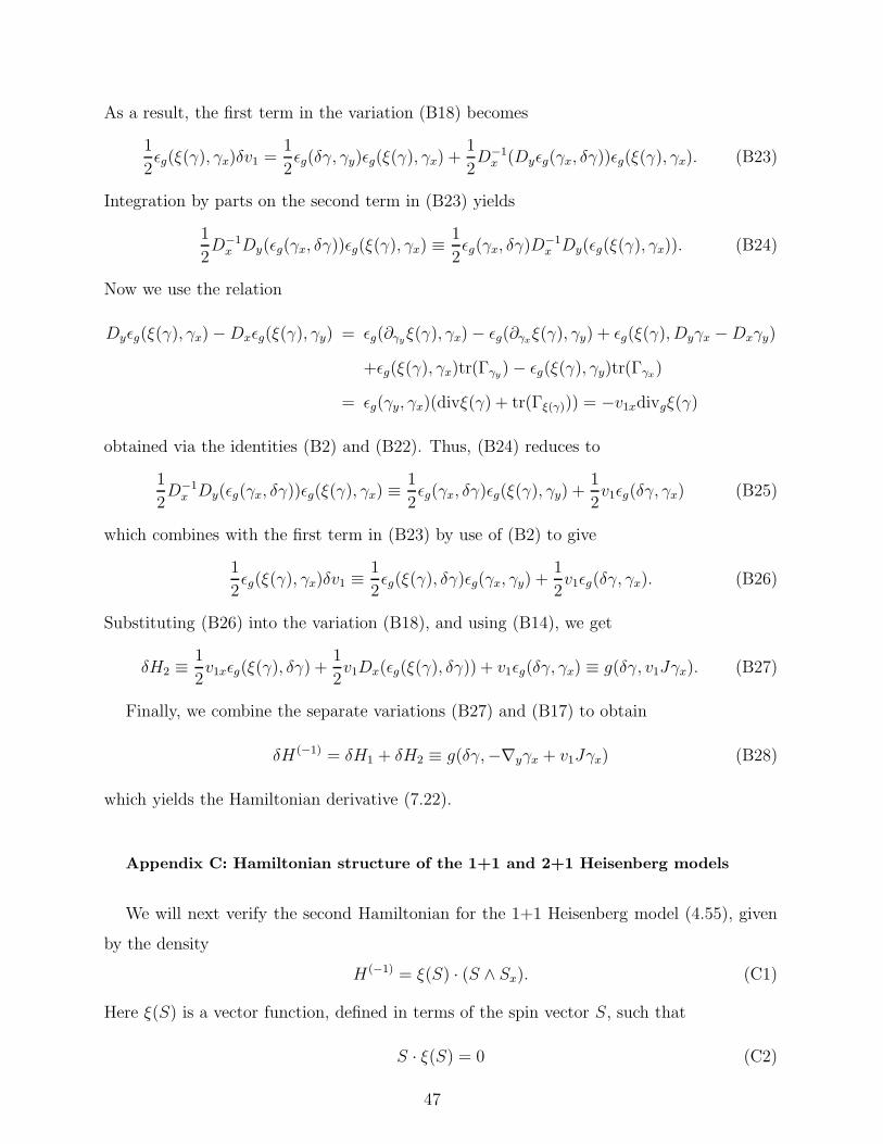
As a result, the first term in the variation (B18) becomes

1

2ǫg(ξ(γ), γx)δv1 =

1

2ǫg(δγ, γy)ǫg(ξ(γ), γx) +

1

2D−1x (Dyǫg(γx, δγ))ǫg(ξ(γ), γx). (B23)

Integration by parts on the second term in (B23) yields

1

2D−1x Dy(ǫg(γx, δγ))ǫg(ξ(γ), γx) ≡

1

2ǫg(γx, δγ)D

−1x Dy(ǫg(ξ(γ), γx)). (B24)

Now we use the relation

Dyǫg(ξ(γ), γx)−Dxǫg(ξ(γ), γy) = ǫg(∂γyξ(γ), γx)− ǫg(∂γxξ(γ), γy) + ǫg(ξ(γ), Dyγx −Dxγy)

+ǫg(ξ(γ), γx)tr(Γγy)− ǫg(ξ(γ), γy)tr(Γγx)

= ǫg(γy, γx)(divξ(γ) + tr(Γξ(γ))) = −v1xdivgξ(γ)

obtained via the identities (B2) and (B22). Thus, (B24) reduces to

1

2D−1x Dy(ǫg(γx, δγ))ǫg(ξ(γ), γx) ≡

1

2ǫg(γx, δγ)ǫg(ξ(γ), γy) +

1

2v1ǫg(δγ, γx) (B25)

which combines with the first term in (B23) by use of (B2) to give

1

2ǫg(ξ(γ), γx)δv1 ≡

1

2ǫg(ξ(γ), δγ)ǫg(γx, γy) +

1

2v1ǫg(δγ, γx). (B26)

Substituting (B26) into the variation (B18), and using (B14), we get

δH2 ≡1

2v1xǫg(ξ(γ), δγ) +

1

2v1Dx(ǫg(ξ(γ), δγ)) + v1ǫg(δγ, γx) ≡ g(δγ, v1Jγx). (B27)

Finally, we combine the separate variations (B27) and (B17) to obtain

δH(−1) = δH1 + δH2 ≡ g(δγ,−∇yγx + v1Jγx) (B28)

which yields the Hamiltonian derivative (7.22).

Appendix C: Hamiltonian structure of the 1+1 and 2+1 Heisenberg models

We will next verify the second Hamiltonian for the 1+1 Heisenberg model (4.55), given

by the density

H(−1) = ξ(S) · (S ∧ Sx). (C1)

Here ξ(S) is a vector function, defined in terms of the spin vector S, such that

S · ξ(S) = 0 (C2)

47

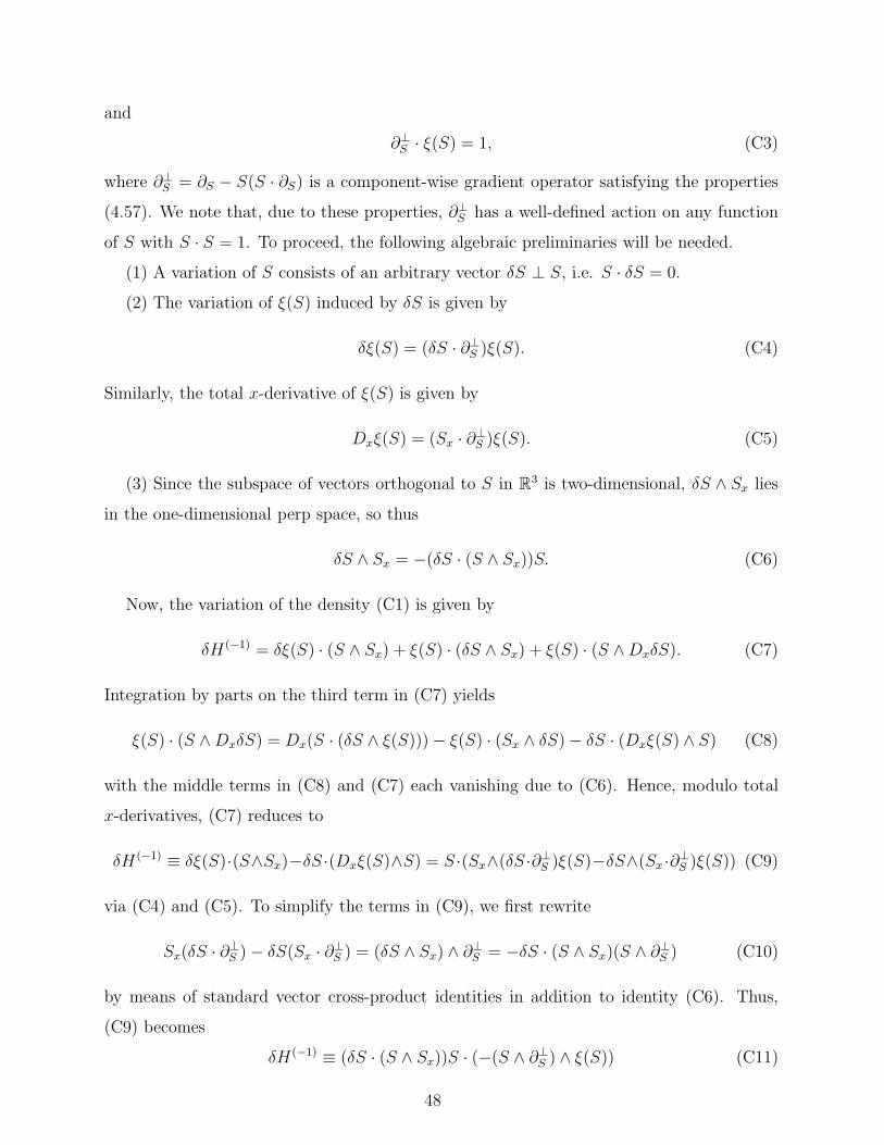
and

∂⊥S · ξ(S) = 1, (C3)

where ∂⊥S = ∂S − S(S · ∂S) is a component-wise gradient operator satisfying the properties

(4.57). We note that, due to these properties, ∂⊥S has a well-defined action on any function

of S with S · S = 1. To proceed, the following algebraic preliminaries will be needed.

(1) A variation of S consists of an arbitrary vector δS ⊥ S, i.e. S · δS = 0.

(2) The variation of ξ(S) induced by δS is given by

δξ(S) = (δS · ∂⊥S )ξ(S). (C4)

Similarly, the total x-derivative of ξ(S) is given by

Dxξ(S) = (Sx · ∂⊥S )ξ(S). (C5)

(3) Since the subspace of vectors orthogonal to S in R3 is two-dimensional, δS ∧ Sx lies

in the one-dimensional perp space, so thus

δS ∧ Sx = −(δS · (S ∧ Sx))S. (C6)

Now, the variation of the density (C1) is given by

δH(−1) = δξ(S) · (S ∧ Sx) + ξ(S) · (δS ∧ Sx) + ξ(S) · (S ∧DxδS). (C7)

Integration by parts on the third term in (C7) yields

ξ(S) · (S ∧DxδS) = Dx(S · (δS ∧ ξ(S)))− ξ(S) · (Sx ∧ δS)− δS · (Dxξ(S) ∧ S) (C8)

with the middle terms in (C8) and (C7) each vanishing due to (C6). Hence, modulo total

x-derivatives, (C7) reduces to

δH(−1) ≡ δξ(S)·(S∧Sx)−δS ·(Dxξ(S)∧S) = S ·(Sx∧(δS ·∂⊥S )ξ(S)−δS∧(Sx ·∂⊥S )ξ(S)) (C9)

via (C4) and (C5). To simplify the terms in (C9), we first rewrite

Sx(δS · ∂⊥S )− δS(Sx · ∂⊥S ) = (δS ∧ Sx) ∧ ∂⊥S = −δS · (S ∧ Sx)(S ∧ ∂⊥S ) (C10)

by means of standard vector cross-product identities in addition to identity (C6). Thus,

(C9) becomes

δH(−1) ≡ (δS · (S ∧ Sx))S · (−(S ∧ ∂⊥S ) ∧ ξ(S)) (C11)

48

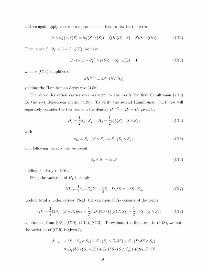
and we again apply vector cross-product identities to rewrite the term

(S ∧ ∂⊥S ) ∧ ξ(S) = ∂⊥S (S · ξ(S))− ξ(S)(∂⊥S · S)− S(∂⊥S · ξ(S)). (C12)

Then, since S · ∂⊥S = 0 = S · ξ(S), we have

S · (−(S ∧ ∂⊥S ) ∧ ξ(S)) = ∂⊥S · ξ(S) = 1 (C13)

whence (C11) simplifies to

δH(−1) ≡ δS · (S ∧ Sx)

yielding the Hamiltonian derivative (4.58).

The above derivation carries over verbatim to also verify the first Hamiltonian (7.13)

for the 2+1 Heisenberg model (7.19). To verify the second Hamiltonian (7.14), we will

separately consider the two terms in the density H(−1) = H1 +H2 given by

H1 =1

2Sx · Sy, H2 =

1

2v1ξ(S) · (S ∧ Sx) (C14)

with

v1x = Sx · (S ∧ Sy) = S · (Sy ∧ Sx). (C15)

The following identity will be useful:

Sy ∧ Sx = v1xS (C16)

holding similarly to (C6).

First, the variation of H1 is simply

δH1 =1

2Sx ·DyδS +

1

2Sy ·DxδS ≡ −δS · Sxy (C17)

modulo total x, y-derivatives. Next, the variation of H2 consists of the terms

δH2 =1

2ξ(S) · (S ∧ Sx)δv1 +

1

2v1Dx(δS · (ξ(S) ∧ S)) + 1

2v1δS · (S ∧ Sx) (C18)

as obtained from (C8), (C10), (C12), (C13). To evaluate the first term in (C18), we note

the variation of (C15) is given by

δv1x = δS · (Sy ∧ Sx) + S · (Sy ∧DxδS) + S · (DyδS ∧ Sx)

≡ Dy(δS · (Sx ∧ S)) +Dx(δS · (S ∧ Sy)) + 2v1xS · δS

49

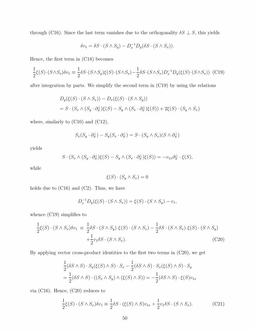
through (C16). Since the last term vanishes due to the orthogonality δS ⊥ S, this yields

δv1 = δS · (S ∧ Sy)−D−1x Dy(δS · (S ∧ Sx)).

Hence, the first term in (C18) becomes

1

2ξ(S)·(S∧Sx)δv1 ≡

1

2δS ·(S∧Sy)ξ(S)·(S∧Sx)−

1

2δS ·(S∧Sx)D−1

x Dy(ξ(S)·(S∧Sx)) (C19)

after integration by parts. We simplify the second term in (C19) by using the relations

Dy(ξ(S) · (S ∧ Sx))−Dx(ξ(S) · (S ∧ Sy))

= S · (Sx ∧ (Sy · ∂⊥S )ξ(S)− Sy ∧ (Sx · ∂⊥S )ξ(S)) + 2ξ(S) · (Sy ∧ Sx)

where, similarly to (C10) and (C12),

Sx(Sy · ∂⊥S )− Sy(Sx · ∂⊥S ) = S · (Sy ∧ Sx)(S ∧ ∂⊥S )

yields

S · (Sx ∧ (Sy · ∂⊥S )ξ(S)− Sy ∧ (Sx · ∂⊥S )ξ(S)) = −v1x∂⊥S · ξ(S),

while

ξ(S) · (Sy ∧ Sx) = 0

holds due to (C16) and (C2). Thus, we have

D−1x Dy(ξ(S) · (S ∧ Sx)) = ξ(S) · (S ∧ Sy)− v1,

whence (C19) simplifies to

1

2ξ(S) · (S ∧ Sx)δv1 ≡ 1

2δS · (S ∧ Sy) ξ(S) · (S ∧ Sx)−

1

2δS · (S ∧ Sx) ξ(S) · (S ∧ Sy)

+1

2v1δS · (S ∧ Sx). (C20)

By applying vector cross-product identities to the first two terms in (C20), we get

1

2(δS ∧ S) · Sy(ξ(S) ∧ S) · Sx −

1

2(δS ∧ S) · Sx(ξ(S) ∧ S) · Sy

=1

2(δS ∧ S) · ((Sx ∧ Sy) ∧ (ξ(S) ∧ S)) = −1

2(δS ∧ S) · ξ(S)v1x

via (C16). Hence, (C20) reduces to

1

2ξ(S) · (S ∧ Sx)δv1 ≡

1

2δS · (ξ(S) ∧ S)v1x +

1

2v1δS · (S ∧ Sx). (C21)

50

Finally, combining (C21) with the middle term in (C18), we get a total x-derivative, so thus

(C18) becomes

δH2 ≡ δS · (v1S ∧ Sx). (C22)

The separate variations (C22) and (C17) then combine to yield the Hamiltonian derivative

(7.22).

[1] S.C. Anco, J. Phys. A: Math. Gen. 36, 8623–8638 (2003).

[2] S.C. Anco, J. Phys. A: Math. Gen. 39, 2043–2072 (2006).

[3] S.C. Anco, SIGMA 2, 044 (2006) 18 pages.

[4] S.C. Anco, in IMA Volumes in Mathematics and its Applications, Vol. 144, Symmetries and

Overdetermined Systems of Partial Differential Equations (AMS) 2007, 223–250.

[5] S.C. Anco, J. Geom. Phys. 58, 1–37 (2008).

[6] E. Barouch, A.S. Fokas, V.G. Papageorgiou, J. Math. Phys. 29, 2628–2633 (1988).

[7] R. Bishop, Amer. Math. Monthly 82, 246–251 (1975).

[8] F. Calogero, Lett. Nuovo Cimento 14, 443–447 (1975).

[9] C. Chen, Z.-X. Zhou, Chin. Phys. Lett., 26, No. 8 (2009) 080504.

[10] A. Doliwa, P.M. Santini, Phys. Lett. A 185, 373–384 (1994).

[11] B. Fuchssteiner, Physica D 13, 387–394 (1984).

[12] H. Guggenheimer, Differential Geometry, McGraw Hill, 1963.

[13] H. Hasimoto, J. Fluid Mech. 51, 477–485 (1972).

[14] M. Lakshmanan, Phys. Lett. A 61, 53–54 (1977).

[15] M. Lakshmanan, R. Myrzakulov, S. Vijayalakshmi, A. Danlybaeva, J. Math. Phys. 39, 3765–

3771 (1998).

[16] J. Langer and R. Perline, Phys. Lett. A 239, 36–40 (1998).

[17] G. Mari Beffa, J. Sanders, J.-P. Wang, J. Nonlinear Sci. 12, 143–167 (2002).

[18] R. Myrzakulov, Spin Systems and Soliton Geometry, Almaty 2001.

[19] R. Myrzakulov, G. Nugmanova, R. Syzdykova, J. Phys. A: Math. Gen. 31, 9535–9545 (1998).

[20] R. Myrzakulov, S. Vijayalakshmi, G.N. Nugmanova, M. Lakshmanan, Phys. Lett. A 233,

391–396 (1997).

51

[21] R. Myrzakulov, S. Vijayalakshmi, R. Syzdykova, M. Lakshmanan, J. Math. Phys. 39, 2122–

2139 (1998).

[22] R. Myrzakulov, A.K. Danlybaeve, G.N. Nugmanova, Theor. Math. Phys. 118, 347–358 (1999).

[23] K. Nakayama, H. Segur, M. Waditi, Phys. Rev. Lett. 69, 2603–2606 (1992).

[24] J. Sanders, J.-P. Wang, Moscow Mathematical Journal 3, 1369–1393 (2003).

[25] N.-H. Chang, J. Shatah, K. Uhlenbeck, Comm. Pure and Applied Math. 53, 0590–0602 (2000).

[26] A.B. Strachan, J. Math. Phys. 33, 2477–2480 (1992).

[27] A.B. Strachan, J. Math. Phys. 34, 243–259 (1993).

[28] C.-L. Terng, K. Uhlenbeck, in Integrable systems, geometry, and topology AMS/IP Stud. Adv.

Math., Vol. 36, Amer. Math. Soc. (Providence, RI) 2006, 235–256.

[29] V.E. Zhakarov, in Solitons, eds. R.K. Bullough and P.J. Caudrey (Springer, Berlin 1980).

[30] Z.H. Zhang, M. Deng, W.Z. Zhao, K. Wu, J. Phys. Soc. Jpn., 75, No. 10 (2006) 104002.

52